How to deal with non-stationary conditions in hydrology using neural networksVirgile TAVER 1, 2

Anne JOHANNET 2

Valérie BORRELL ESTUPINA 1

Séverin PISTRE 1

(1) HSM, HydroSciences Montpellier, UMR5569, Université de Montpellier 2, France(2) Ecole des Mines d’Alès, France

Made possible by a collaboration

IAHS General Assembly in Göteborg - July 2013

Session : Testing simulation and forecasting models in non-stationary conditions

1

Neural Networks (NN)

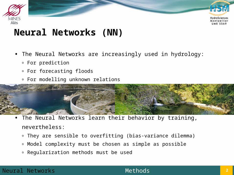
• The Neural Networks are increasingly used in hydrology: o For predictiono For forecasting floodso For modelling unknown relations

• The Neural Networks learn their behavior by training, nevertheless:o They are sensible to overfitting (bias-variance dilemma)o Model complexity must be chosen as simple as possibleo Regularization methods must be used

Neural Networks Methods Results Conclusion 2

Neural Networks

• Neuron definition:o Weighted sumo Non-linear function (f)

• Neural Network architecture:o Multilayer perceptron

➥Universal approximation

➥ Parsimony (for statistical models)

Neural Networks Methods Results Conclusion 3

Neural Network: design methodology

• Minimization of the quadratic error during training by Levenberg-Marquardt rule

• Data base utilization:o One (sub)-set for training (Pi, i=1,5)

o One (sub)-set for stopping (early stopping with records ≠(Pi, i=1,5))o One (sub)-set for test (in level 3), different from training and stop sets

• Complexity selection o Definition of architecture using cross-validation (included inside the training period) :

• Input variables (ui)

• Number of hidden layers and hidden neurons

o Selection using Nash criterion

Neural Networks Methods Results Conclusion 4

3 ways of modelling

• 3 models can be investigated regarding the postulated model

• For example let us consider an analogy : calculate the price of a “baguette”, 3

methods can used to estimate such a price :

1. Take into account the price of primary ingredients (flour, water …), energy, and

compute the price for a specific recipe

2. If the state measurement is good: take into account the measured price yesterday,

and anticipate a one-day evolution

3. If the state measurement isn't good: take into account the estimated price

yesterday, and anticipate evolution

Neural Networks Methods Results Conclusion 5

3 ways of modelling

• 3 models can be investigated regarding the postulated model:

1. Computing discharge from rainfall and physics

2. Computing discharge from the state measurement

3. Computing discharge from the state estimation

Neural Networks Methods Results Conclusion 6

Static system modelling

Dynamic system modelling

=> Non-directed NN model

=> Static NN model

=> Directed NN model

1 NN model for each postulated model

Un-directedNN model

StaticNN model

DirectedNN model

• Postulated model 1

• Postulated model 2: noise on the state

• Postulated model 3 : noise on the measurement

φ

q-1

u (k)

yp (k)

b (k+1)

yp(k+1)φRNu (k)

yp (k)g(k+1)

yp: observed output of the physical process

u (k): observed input of the physical process (rain)

b (k): noise

φ

q-1

u (k)xp (k)

b (k+1)

yp(k+1)

xp (k+1)

φu (k) yp(k+1)φRNu (k) g(k+1)

φRN

q-1

u (k)g (k)

g (k+1)

Neural Networks Methods Results Conclusion 7

1 NN model for each postulated model

Un-directedNN model

StaticNN model

DirectedNN model

• Postulated model 1

• Postulated model 2: noise on the state

• Postulated model 3 : noise on the measurement

φ

q-1

u (k)

yp (k)

b (k+1)

yp(k+1)φRNu (k)

yp (k)g(k+1)

yp: observed output of the physical process

u (k): observed input of the physical process (rain)

b (k): noise

φ

q-1

u (k)xp (k)

b (k+1)

yp(k+1)

xp (k+1)

φu (k) yp(k+1)φRNu (k) g(k+1)

φRN

q-1

u (k)g (k)

g (k+1)

Neural Networks Methods Results Conclusion 8

1 NN model for each postulated model

Non-directedNN model

StaticNN model

DirectedNN model

• Postulated model 1

• Postulated model 2: noise on the state

• Postulated model 3 : noise on the measurement

φ

q-1

u (k)

yp (k)

b (k+1)

yp(k+1)φRNu (k)

yp (k)g(k+1)

yp: observed output of the physical process

u (k): observed input of the physical process (rain)

b (k): noise

φ

q-1

u (k)xp (k)

b (k+1)

yp(k+1)

xp (k+1)

φu (k) yp(k+1)φRNu (k) g(k+1)

φRN

q-1

u (k)g (k)

g (k+1)

Neural Networks Methods Results Conclusion 9

1 NN model for each postulated model

Non-directedNN model

StaticNN model

DirectedNN model

• Postulated model 1

• Postulated model 2: noise on the state

• Postulated model 3 : noise on the measurement

φ

q-1

u (k)

yp (k)

b (k+1)

yp(k+1)φRNu (k)

yp (k)g(k+1)

yp: observed output of the physical process

u (k): observed input of the physical process (rain)

b (k): noise

φ

q-1

u (k)xp (k)

b (k+1)

yp(k+1)

xp (k+1)

φu (k) yp(k+1)φRNu (k) g(k+1)

φRN

q-1

u (k)g (k)

g (k+1)

Neural Networks Methods Results Conclusion 10

3 ways to deal with non stationary

• How to adapt the model to the changing environment and process?

o Changing process or environment• The observed data are used to adapt parameter values at

different time steps Adaptativity

o The observed data are used as input data at different time step

Directed Model• The observed data are used to modify inaccurate inputs at

different time steps Data AssimilationA variationnal approach is used in this work to modify rainfalls, temperature and snow at each time step

Neural Networks Methods Results Conclusion 11

Possible on the 3 models

Only for Directed

model

Possible on the 3 models

Application:- Fernow watershed,- Durance watershed

Only models able to represent dynamic systems were developed :

Directed (non-recurrent model)

Non-Directed (recurrent model)

Neural Networks Methods Results Conclusion 12

Non-directedNN model

DirectedNN modelφRNu (k)

yp (k)g(k+1)

φRN

q-1

u (k)g (k)

g (k+1)

2 ways of dealing with non-stationary : No option Adaptativity Assimilation

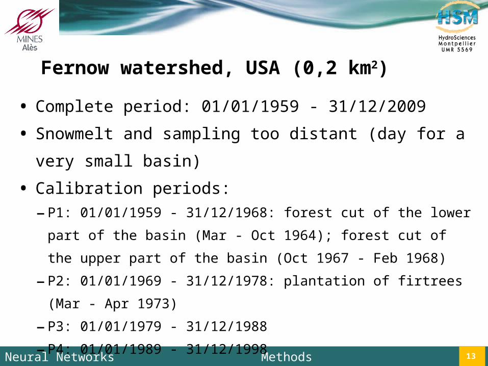
Fernow watershed, USA (0,2 km2)

Neural Networks Methods Results Conclusion 13

• Complete period: 01/01/1959 - 31/12/2009

• Snowmelt and sampling too distant (day for a very small basin)

• Calibration periods: – P1: 01/01/1959 - 31/12/1968: forest cut of the lower part of the basin (Mar

- Oct 1964); forest cut of the upper part of the basin (Oct 1967 - Feb 1968)

– P2: 01/01/1969 - 31/12/1978: plantation of firtrees (Mar - Apr 1973)

– P3: 01/01/1979 - 31/12/1988

– P4: 01/01/1989 - 31/12/1998

– P5: 01/01/1999 - 31/12/2008

Fernow model

Neural Networks Methods Results Conclusion 14

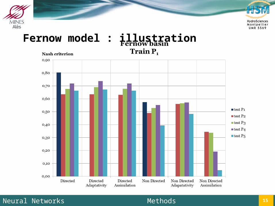
Fernow model : illustration

Neural Networks Methods Results Conclusion 15

Durance watershed, France ( 2170 km2)

Neural Networks Methods Results Conclusion 16

• Observed non-stationary: Temperature higher implying decrease of glaciers

• Discharge during spring due to snowmelt

• Complete period: 01/01/1904 - 30/12/2010

• Calibration periods:

– P1: 01/01/1904 - 31/12/1924

– P2: 01/01/1925 - 31/12/1945

– P3: 01/01/1946 - 31/12/1966

– P4: 01/01/1967 - 31/12/1987

– P5: 01/01/1988 - 31/12/2008

Durance model

Neural Networks Methods Results Conclusion 17

Rain 7j

Temp 10j

PET 4j

Qcalc 2j

Hidden Layers 3

Architecture defined on P1

Durance model : illustration

Neural Networks Methods Results Conclusion 18

During the spring period, discharge of the Durance is due to snowmelt.To take into account this process, positive temperatures of winter and spring are preserved (from 1st of January to 30th of June). All the other temperature are set to zero.

Durance model : illustration

Neural Networks Methods Results Conclusion 19

Model Input Temperature

Assimilation on

Directed The supplied ones

Rainfall

Non-Directed

The supplied ones

Rainfall, Temperature, PET

Non directed

Snowmelt Rainfall

Fernow Durance

Neural Networks Methods Results Conclusion 20

Directed, no option

With the Directed model with Adaptativity or Assimilation on the Fernow catchment :•Improvement of the Nash•But decrease of the performance on the low flows on some periods

Not a Gain, nor a deterrioration on the Durance catchment

Fernow Durance

Neural Networks Methods Results Conclusion 21

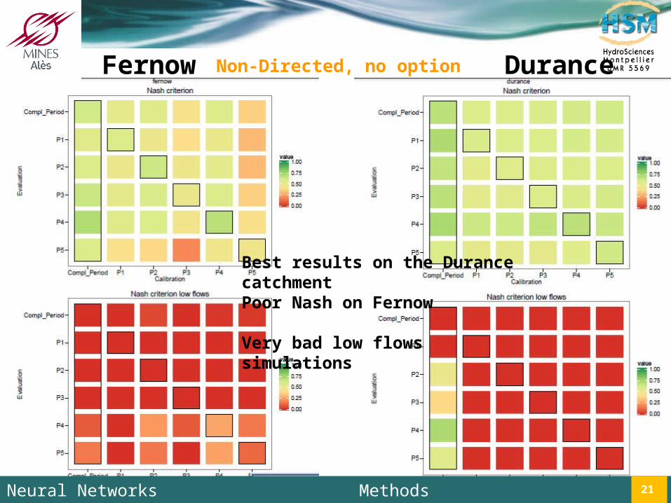
Non-Directed, no option

Best results on the Durance catchmentPoor Nash on Fernow

Very bad low flows simulations

Neural Networks Methods Results Conclusion 22

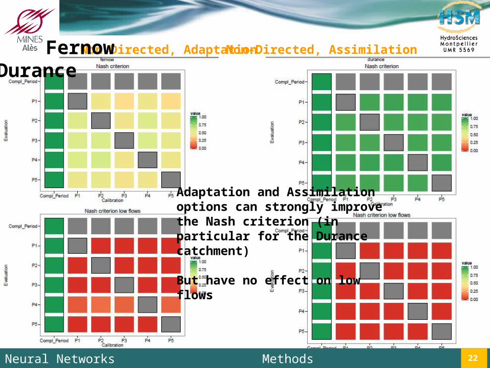
Adaptation and Assimilation options can strongly improve the Nash criterion (in particular for the Durance catchment)

But have no effect on low flows

Non-Directed, Adaptation Non-Directed, AssimilationFernow Durance

Neural Networks Methods Results Conclusion 23

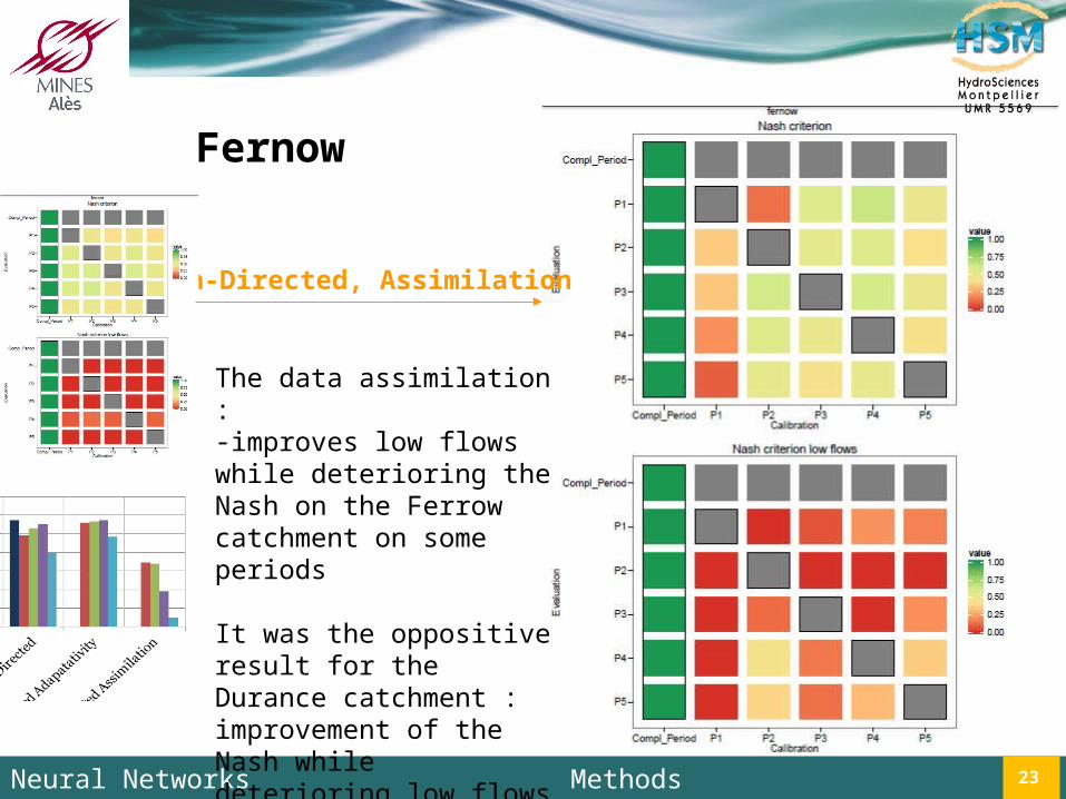
Fernow

Non-Directed, Assimilation

The data assimilation : -improves low flows while deterioring the Nash on the Ferrow catchment on some periods

It was the oppositive result for the Durance catchment : improvement of the Nash while deterioring low flows on (previous slide)

Neural Networks Methods Results Conclusion 24

Durance

Non-Directed, no Option, T°

The treatment of temprature (Snowmelt) improves the Nash criterionBad simulations on low flows

Non-Directed, Assimilation, T°

Non-Directed, no Option

Conclusions

Neural Networks Methods Results Conclusion 25

• The best way (reliable , simple, easy) to adapt the model to the changing

environment consists in using the Directed Model (feedforward model)

• When using Directed Model, there has been no appreciable progress when using

adaptativity or assimilation

• When using Non-Directed model, the improvement provided by adapatativity and

data assimilation can be high

• Neural Network Modelling is more efficient for the largest studied catchment

• Work on progres : data assimilation must be studied more deeply (some parameters

to adjust), the criteria used for otpimization have to be complixified (to avoid that

the improvement on high flows appears when decreasing performance on low flows

and vice versa) Thank you for your time