how much fbmc/oqam is better than fbmc/qam? a tentative response using the pops...
TRANSCRIPT
Research ArticleHow Much FBMCOQAM Is Better than FBMCQAMA Tentative Response Using the POPS Paradigm
Wafa Khrouf Mohamed Siala and Fatma Abdelkefi
Mediatron Laboratory Higher School of Communications of Tunis (SUPrsquoCOM) 2083 Ariana Tunisia
Correspondence should be addressed to Wafa Khrouf wafakhroufsupcomtn
Received 28 July 2017 Revised 3 November 2017 Accepted 20 December 2017 Published 10 April 2018
Academic Editor Malte Schellmann
Copyright copy 2018 Wafa Khrouf et al This is an open access article distributed under the Creative Commons Attribution Licensewhich permits unrestricted use distribution and reproduction in any medium provided the original work is properly cited
A major trend of the current research in 5G is to find well time and frequency localized waveforms dedicated to non-orthogonalwireless multi-carrier systems The ping-pong optimized pulse shaping (POPS) paradigm was proposed as a powerful techniqueto generate a family of waveforms ensuring an optimal signal to interference plus noise ratio (SINR) at the receiver In this paperwe derive for the first time the analytical expression of the SINR for FBMCOQAM systems We then adopt the POPS algorithmin the design of optimum transmit and receive waveforms for FBMCOQAM with respect to the SINR criterion For relativelyhigh dispersions numerical results show that the optimized waveforms provide a gain of 7 dB in terms of SINR compared to thePHYDYASwaveformThey also show that the obtainedwaveforms offer better out-of-band (OOB) emissionswith regard to those ofthe IOTAwaveform Furthermore we notice that FBMCOQAM systems present a gain of 4 dB in SINR compared to FBMCQAMsystems when both operate at their time-frequency lattice critical densities However FBMCQAM systems can guarantee with areduced computational complexity a comparable performance to FBMCOQAM systems in terms of SINR when their spectralefficiency is relatively reduced by less than 5
1 Introduction
Orthogonal frequency division multiplexing (OFDM) sys-tems have witnessed a considerable interest in the last decade[1] However in their present form they are deemed inapt ofguaranteeing the required quality of service (QoS) in severalnew challenging applications brought by 5G systems Thisinaptitude is due to many factors Among them we can citethe strong spectral leakage which can only be controlledwith strict frequency synchronization As a consequence anylack of perfect frequency synchronization causes importantintercarrier interference (ICI) Besides this incapacity isa result of the intersymbol interference (ISI) when theactual channel delay spread exceeds the cyclic prefix (CP)duration andor strict time synchronization is relaxed to savesignalling resources and delays [2]
To overcome OFDM limitations and meet 5G require-ments several European projects have been launched recent-ly such as ldquomobile and wireless communications enablersfor twenty-twenty (2020) information societyrdquo (METIS) [3]ldquoflexible air interface for scalable service delivery within
wireless communication networks of the 5th generationrdquo(FANTASTIC5G) [4] ldquoenhanced multi-carrier techniquesfor professional ad-hoc and cell-based communicationsrdquo(EMPHATIC) [5] and ldquo5th generation non-orthogonalwaveforms for asynchronous signallingrdquo (5GNOW) [6] Inthe 5GNOW project for instance various modulations havebeen suggested [7] namely filter bankmulti-carrier (FBMC)generalized frequency division multiplexing (GFDM) anduniversal filtered multi-carrier (UFMC) Among these mul-tiple access techniques FBMC seems to be a good candidatefor 5G systems In the literature many researches shed lighton the advantages of FBMCwith offset quadrature amplitudemodulation (FBMCOQAM) systems compared to OFDMsystems Among these advantages one can cite their robust-ness to channel time and frequency spreading [8] since theirwaveforms are well localized in time and frequency HoweverFBMCOQAM implementation and analytical derivation ofthe SINR are more complex than those of OFDM
In this paper we focus on FBMCOQAM systems whichare also known as OFDMOQAM and staggered multitone(SMT) [9] They consist in transmitting separately and
HindawiWireless Communications and Mobile ComputingVolume 2018 Article ID 4637181 14 pageshttpsdoiorg10115520184637181
2 Wireless Communications and Mobile Computing
alternately in each subcarrier the in-phase and quadraturecomponents of complex symbols used in quadrature ampli-tude modulation (QAM) We believe that there are a limitednumber of studies which have attempted to derive the SINRanalytical expression of FBMCOQAM systems [10ndash12] In[10] the SINR is derived for known transmitter (Tx) andreceiver (Rx) waveforms On the other hand in [11] theauthors calculate the signal to interference ratio (SIR) fora channel with a carrier frequency offset (CFO) whereasin [12] the authors derive the SIR for a channel with aCFO andor a time offset (TO) In contrast in this paperwe derive the analytical expression of the SINR for multi-carrier transmissions in the case of highly time and frequencydispersive channels Once the SINR analytical expression isestablished we seek the appropriate TxRx waveforms whichoptimize the SINR To this end we extend the applicationof the POPS paradigm adopted for FBMCQAM systems in[13] to FBMCOQAM systems The POPS algorithm firstlyintroduced in [14] has the merit of being very effective inthe optimization of the transmit and receive waveforms It isan iterative algorithm which enables simple and offline opti-mization of the waveforms at the TxRx sides by maximizingthe SINR
The optimal TxRx waveforms resulting from POPS arerobust against the ISI and ICI incurred by mobile radiocommunication propagation channels However the imagi-nary part of the interference known as intrinsic interference[15 16] is inherent to FBMCOQAM systems To accountfor it channel estimation is always required The intrinsicinterference remaining after channel estimation cannot beneglected unless the channel is not severely dispersive insingle-input single-output (SISO) systems or linear spatialequalization schemes are used inmoderately dispersive chan-nels in multiple-input multiple-output (MIMO) systemsMoreover if spatial equalization other than linear schemes isused in MIMO a complex equalization process is required toaccount for the intrinsic interference Keeping this in mindwe exclusively focus in this paper on SISO systems and targetthe optimization of TxRx waveforms in this context
Our main contributions in this paper are the following
(i) We provide an analytical expression of the SINR forFBMCOQAM systems in arbitrary channel condi-tions for whatever TxRx waveforms
(ii) We compare theoretically the performances ofFBMCQAM and FBMCOQAM systems in an arbi-trary propagation framework
(iii) We present and detail the performance of FBMCQAM systems with lattice densities below or equal to1
(iv) We quantify potential gains that can be realized byFBMCOQAM systems with respect to FBMCQAMsystems using identical andor different lattice densi-ties
(v) We compare the performances of POPS waveformswith respect to physical layer for dynamic access andcognitive radio (PHYDYAS) and isotropic orthogonal
transform algorithm (IOTA) waveforms in FBMCOQAM systems
This paper is organized as follows In Section 3 wepresent the adopted system model for FBMCOQAM andFBMCQAMsystemsThen we focus on the derivation of theuseful interference and noise powers in Section 4 and derivethe SINR expression for FBMCOQAM systems in Section 5In Section 6 we describe the POPS algorithm suitable forthe design of optimal waveforms We dedicate Section 7 tothe illustration of the obtained analytical results Finally wepresent conclusion and perspectives to this work in Section 8
2 Notations
Boldface lower and upper case letters refer to vectors andmatrices respectively and 119872119896119897 refers interchangeably to the(119901 119902)th element of the matrix 119872 The superscripts sdotlowast sdot119879 andsdotminus1 denote the conjugate of a function the transpose of avector and the inverse of a matrix respectivelyWe denote byE[sdot] the expectation operator byRsdot the real-part operatorby | sdot | the absolute value and by ⟦119899119898⟧ the set of integersbetween 119899 and 119898 where 119899 le 119898 We denote by ⟨119909 119910⟩ =int 119909lowast(119905)119910(119905)119889119905 the Hermitian scalar product by ⟨119909 119910⟩R =R⟨119909 119910⟩ the real scalar product and by 119909 = radic⟨119909 119909⟩ =radic⟨119909 119909⟩R = radicint |119909(119905)|2119889119905 the norm of 1199093 System Model
In this section we consider a general FBMC system modelin its continuous-time version We denote by 119879 the FBMC(QAMorOQAM) symbol period by 119865 the frequency separa-tion between adjacent subcarriers by 119865119879 the time-frequencyoccupancy of each transmitted symbol and by Δ = 1119865119879the lattice density To preserve the same spectral efficiency asin FBMCQAM FBMCOQAM should use twice the latticedensity since real symbols are transmitted in place of complexsymbols Hence to have a critical density the lattice densityshould be equal to Δ = 2 in FBMCOQAM when Δ = 1 inFBMCQAM
The FBMC transmitted signal can be written under thefollowing expression
119890 (119905) = sum119898119899
119886119898119899120593119898119899 (119905) (1)
where 119898 119899 isin Z 119886119898119899 is the data symbol transmitted at time119899119879 and frequency119898119865 and120593119898119899 (119905) = 119890119895120579119898119899120593 (119905 minus 119899119879) 1198901198952120587119898119865119905 (2)
refers to the phase time and frequency shifted version ofthe transmitter prototype waveform 120593(119905) used to transmita symbol 119886119898119899 The phase shift 120579119898119899 is used in FBMCOQAMto guarantee the orthogonality between the in-phase andquadrature phase components of the complex symbols usedin FBMCQAMwith respect to the real scalar product ⟨sdot sdot⟩RIn practice we take 120579119898119899 = (119898 + 119899)1205872 for FBMCOQAMsystems and 120579119898119899 = 0 for FBMCQAM systems
Wireless Communications and Mobile Computing 3
The received signal is given by119903 (119905) = sum119898119899
119886119898119899120593119898119899 (119905) + 119899 (119905) (3)
where 120593119898119899(119905) = int 119888(120591 119905)120593119898119899(119905 minus 120591)119889120591 is the channel-distortedversion of 120593119898119899(119905) 119888(120591 119905) is the channel impulse response(CIR) at time 119905 and 119899(119905) is a base-band complex additivewhiteGaussian noise (AWGN)with zeromean and two-sidedpower spectral density (PSD)1198730 For simplification reasonswe consider a channel with a finite number of paths 119871 and aCIR equal to 119888(120591 119905) = sum119871minus1
119897=0 1198881198971198901198952120587]119897119905120575(120591 minus 120591119897) where 119888119897 ]119897 and120591119897 are respectively the amplitude frequency Doppler shiftand time delay shift of the 119897th path The paths amplitudes 119888119897119897 = 0 119871 minus 1 are assumed to be centered and uncorrelatedrandom complex Gaussian variables with average powers120587119897 = E[|119888119897|2]4 Useful Interference and Noise Powers
In this section we evaluate the useful interference and noisepowers of both FBMCOQAM and FBMCQAM systemsusing the same propagation channel conditions
41 FBMCOQAM System In FBMCOQAM systems deci-sion variables are calculated using a real scalar productTherefore in nondispersive channels where the interferenceis purely imaginary perfect orthogonality is achieved Unfor-tunately in the more general case of dispersive channels astreated in this paper the real part of the interference becomesan integral part of the decision variable on symbol 119886119896119897 in (1)which is given by Λ 119896119897 = ⟨119890119895120594119896119897120595119896119897 119903⟩R (4)
where 120595119896119897(119905) = 119890119895120579119896119897120595(119905 minus 119897119879)1198901198952120587119896119865119905 is the phase time andfrequency shifted version of the receiver prototypewaveform120595(119905) used for the demodulation of the real symbol 119886119896119897 andthe phase 120594119896119897 is used to compensate even partially the phaseshift incurred by the channel at the time-frequency position(119897119879 119896119865) occupied by 119886119896119897 Choosing a phase shift for 120595119896119897(119905)equal to 120579119896119897 = (119896 + 119897)1205872 guarantees a quasi-orthogonalitybetween the alternately transmitted in-phase and quadraturephase components of FBMCQAM whatever the consideredreal symbol 119886119896119897 to be demodulated Therefore the decisionvariables characteristics are invariant by time and frequencytranslations within the time-frequency lattice keeping thetime-frequency lattice unchanged Making this necessaryassumption we can without loss of generality focus on theevaluation of the SINR for symbol 11988600 The decision variableon 11988600 can be expanded into three terms asΛ 00 = 11988600 ⟨1198901198951205940012059500 12059300⟩R⏟⏟⏟⏟⏟⏟⏟⏟⏟⏟⏟⏟⏟⏟⏟⏟⏟⏟⏟⏟⏟⏟⏟⏟⏟⏟⏟⏟⏟⏟⏟⏟⏟⏟⏟⏟⏟
11988000+ sum119898119899(119898119899) =(00)
119886119898119899 ⟨1198901198951205940012059500 120593119898119899⟩R⏟⏟⏟⏟⏟⏟⏟⏟⏟⏟⏟⏟⏟⏟⏟⏟⏟⏟⏟⏟⏟⏟⏟⏟⏟⏟⏟⏟⏟⏟⏟⏟⏟⏟⏟⏟⏟⏟⏟⏟⏟⏟⏟⏟⏟⏟⏟⏟⏟⏟⏟11986800+ ⟨1198901198951205940012059500 119899⟩R⏟⏟⏟⏟⏟⏟⏟⏟⏟⏟⏟⏟⏟⏟⏟⏟⏟⏟⏟⏟⏟⏟⏟⏟⏟
11987300
(5)
where11988000 11986800 and11987300 are the useful interference and noiseterms respectively
Conditional on a given realization of the CIR 119888(120591 119905)the average powers of the useful and interference terms areexpressed as
119875119888119880 = E [1198802
00] = E [119886200] (R 119890minus11989512059400 ⟨12059500 12059300⟩)2 (6)
119875119888119868 = E [119868200]= E [1198862
119898119899] sum119898119899(119898119899) =(00)
(R 119890minus11989512059400 ⟨12059500 120593119898119899⟩)2 (7)
The expression in (7) results from the uncorrelated nature ofthe real transmitted symbols 119886119898119899 The average transmittedenergy corresponding to symbol 119886119898119899 is given by 119864119904 =E[(119886119898119899120593)2] = E[1198862
119898119899]1205932 Let 119864 be the mean energy of acomplex symbol in the case of FBMCQAM systems thenfor comparison purposes we assume that 119864119904 = 1198642 whichmeans that E[1198862
119898119899] = 1198641199041205932 = 11986421205932To calculate the SINR an averaging over the channel real-
izations is needed This step is precisely the most challengingand complicated step in FBMCOQAM systems since inaddition to 120593119898119899(119905) the phase compensation term 11989011989512059400 is alsodependent on the same channel realizations For an optimumchoice of the compensation factor maximizing the SINR weuse
11989011989512059400 = ⟨12059500 12059300⟩1003816100381610038161003816⟨12059500 12059300⟩1003816100381610038161003816 (8)
which captures the phase shift incurred by the channelrealization on the decision variable of symbol 11988600 prior tocasting to the real part This is the ideal choice of 12059400 thatallows a compensation with the exact phase shift experiencedby the symbol which is caused by the channel Howeverthis choice makes the optimization step intractable since theexpected form of the SINR will not be a generalized Rayleighquotient but the ratio of two quaternary forms on each of thesearched transmitter and receiver waveforms For a furthersimplification of the optimization problem with an expectedtractable form of the SINR we can use the transfer functionof the channel 119862(119891 119905) = sum119871minus1
119897=0 1198881198971198901198952120587]119897119905119890minus1198952120587120591119897119891 which is theFourier transform of the CIR 119888(120591 119905) with respect to 120591 anduse the compensation factor
11989011989512059400 = 119862 (0 0)|119862 (0 0)| = sum119871minus1119897=0 11988811989710038161003816100381610038161003816sum119871minus1119897=0 11988811989710038161003816100381610038161003816 (9)
By averaging expressions (6) and (7) on the realizations of thechannel the useful and interference powers are respectivelygiven by
119875119880 = E [119875119888119880] = 1198642 100381710038171003817100381712059310038171003817100381710038172E [(R 119890minus11989512059400 ⟨12059500 12059300⟩)2] (10)
119875119868 = E [119875119888119868 ]
= 1198642 100381710038171003817100381712059310038171003817100381710038172 sum119898119899(119898119899)=(00)
E [(R 119890minus11989512059400 ⟨12059500 120593119898119899⟩)2] (11)
4 Wireless Communications and Mobile Computing
Let119864 = 119864sum119871minus1119897=0 120587119897 be the average energy received per complex
symbol and let 119897 = 120587119897sum119871minus1119897=0 120587119897 be the normalized multipath
power profile of the channel with sum119871minus1119897=0 119897 = 1 Using the
results of Appendix 1 we can write
119875119880 = 1198644 100381710038171003817100381712059310038171003817100381710038172 [119871minus1sum119896=0
119896
sdot ∬12059500 (119905) 120595lowast00 (119904) 120593lowast
00 (119905 minus 120591119896) 12059300 (119904 minus 120591119896) 1198901198952120587]119896(119904minus119905)119889119905 119889119904+R 119871minus1sum
119896119897=0
119896119897
sdot∬120595lowast00 (119905) 120595lowast
00 (119904) 12059300 (119905 minus 120591119896) 12059300 (119904 minus 120591119897) 1198901198952120587(]119896119905+]119897119904)119889119905 119889119904]
(12)
119875119868 = 1198644 100381710038171003817100381712059310038171003817100381710038172 sum119898119899(119898119899) =(00)
[119871minus1sum119896=0
119896
sdot ∬12059500 (119905) 120595lowast00 (119904) 120593lowast
119898119899 (119905 minus 120591119896) 120593119898119899 (119904 minus 120591119896) 1198901198952120587]119896(119904minus119905)119889119905 119889119904+R 119871minus1sum
119896119897=0
119896119897
sdot∬120595lowast00 (119905) 120595lowast
00 (119904) 120593119898119899 (119905 minus 120591119896) 120593119898119899 (119904 minus 120591119897) 1198901198952120587(]119896119905+]119897119904)119889119905 119889119904]
(13)
To extend the obtained results to more general diffusechannels obeying the wide sense stationary uncorrelatedscattering (WSSUS) property [17] we consider the asymptoticconfiguration where 119871 rarr +infin in (12) Denoting by 119878(120591 ])the scattering function of the channel and by 119878(120591 ]) =119878(120591 ])∬119878(120591 ])119889120591 119889] its normalized version we can rewrite119875119880 and 119875119868 in a more general form as
119875119880 = 1198644 100381710038171003817100381712059310038171003817100381710038172 [∬119878 (120591 ]) (∬120595 (119905) 120595lowast (119904) 120593lowast (119905 minus 120591)sdot 120593 (119904 minus 120591) 1198901198952120587](119904minus119905)119889119905 119889119904 ) 119889120591 119889]
+R ∬∬119878 (1205911 ]1) 119878 (1205912 ]2)sdot (∬120595lowast (119905) 120595lowast (119904) 120593 (119905 minus 1205911)sdot 120593 (119904 minus 1205912) 1198901198952120587(]1119905+]2119904)119889119905 119889119904) 11988912059111198891205912119889]1119889]2]
(14)
119875119868 = 1198644 100381710038171003817100381712059310038171003817100381710038172 sum119898119899(119898119899) =(00)
[∬119878 (120591 ]) (∬120595 (119905) 120595lowast (119904) 120593lowast119898119899 (119905 minus 120591)
sdot 120593119898119899 (119904 minus 120591) 1198901198952120587](119904minus119905)119889119905 119889119904) 119889120591 119889]+R ∬∬119878 (1205911 ]1) 119878 (1205912 ]2)
sdot (∬120595lowast (119905) 120595lowast (119904) 120593119898119899 (119905 minus 1205911)sdot 120593119898119899 (119904 minus 1205912) 1198901198952120587(]1119905+]2119904)119889119905 119889119904) 11988912059111198891205912119889]1119889]2 ]
(15)
The noise power is given by
119875119873 = E [(R 119890minus11989512059400 ⟨12059500 119899⟩)2] (16)
where 119890minus11989512059400⟨12059500 119899⟩ is a circular random complex Gaussianvariable which is independent of 119890minus11989512059400 and has the samevariance as ⟨12059500 119899⟩ ThusR119890minus11989512059400⟨12059500 119899⟩ is a random realGaussian variable which has half the variance of ⟨12059500 119899⟩Accordingly
119875119873 = 12E [1003816100381610038161003816⟨12059500 119899⟩10038161003816100381610038162] (17)
Since the noise is white with autocorrelation function119877119899119899(120591) = 1198730120575(120591) where 120575(sdot) is the Dirac delta function wecan write
E [1003816100381610038161003816⟨12059500 119899⟩10038161003816100381610038162]= E [(int120595lowast
00 (119905) 119899 (119905) 119889119905)lowast (int120595lowast00 (119904) 119899 (119904) 119889119905)]
= ∬12059500 (119905) 120595lowast00 (119904)E [119899lowast (119905) 119899 (119904)] 119889119905 119889119904
= 1198730100381710038171003817100381712059500
10038171003817100381710038172 (18)
Consequently the noise power can be expressed as
119875119873 = 11987302 100381710038171003817100381712059510038171003817100381710038172 (19)
42 FBMCQAM System The SINR expression for FBMCQAM systems was derived in [13 14] in the case of con-tinuous- and discrete time respectively In this section webriefly present the main steps considered to find its analyticalexpression in the case of continuous signals
The decision variable on complex symbol 119886119896119897 bearingsimultaneously both in-phase and quadrature phase compo-nents uses the conventional Hermitian scalar product andhas the following expression
Λ 119896119897 = ⟨120595119896119897 119903⟩ = int120595lowast119896119897 (119905) 119903 (119905) 119889119905 (20)
where 120595119896119897(119905) = 120595(119905 minus 119897119879)1198901198952120587119896119865119905 is the time and frequencyshifted version of the receiver prototype waveform120595(119905) usedfor the demodulation of the complex symbol 119886119896119897
Again and as before for FBMCOQAM we will evaluatewithout loss of generality the SINR for symbol 11988600 Thedecision variable on 11988600 can be expanded into three terms as
Λ 00 = 11988600 ⟨12059500 12059300⟩⏟⏟⏟⏟⏟⏟⏟⏟⏟⏟⏟⏟⏟⏟⏟⏟⏟⏟⏟⏟⏟⏟⏟⏟⏟11988000
+ sum119898119899(119898119899)=(00)
119886119898119899 ⟨12059500 120593119898119899⟩⏟⏟⏟⏟⏟⏟⏟⏟⏟⏟⏟⏟⏟⏟⏟⏟⏟⏟⏟⏟⏟⏟⏟⏟⏟⏟⏟⏟⏟⏟⏟⏟⏟⏟⏟⏟⏟⏟⏟11986800+ ⟨12059500 119899⟩⏟⏟⏟⏟⏟⏟⏟⏟⏟⏟⏟⏟⏟
11987300
(21)
where11988000 11986800 and11987300 are the useful interference and noiseterms respectively
Wireless Communications and Mobile Computing 5
Conditional on a given realization of the CIR 119888(120591 119905) theaverage powers of the useful and interference terms are givenby
119875119888119880 = E [100381610038161003816100381611988000
10038161003816100381610038162] = E [119886200] 1003816100381610038161003816⟨12059500 12059300⟩10038161003816100381610038162 (22)
119875119888119868 = E [10038161003816100381610038161198680010038161003816100381610038162] = E [1198862
119898119899] sum119898119899(119898119899) =(00)
1003816100381610038161003816⟨12059500 120593119898119899⟩10038161003816100381610038162 (23)
The expression in (23) results from the uncorrelated natureof the complex transmitted symbols 119886119898119899 Since the averagetransmitted energy of 119886119898119899 is 119864 = E[(119886119898119899120593)2] = E[1198862
119898119899]1205932we conclude that E[1198862
119898119899] = 1198641205932 By averaging theexpressions in (22) and (23) on the realizations of the channelwe obtain
119875119880 = 119864100381710038171003817100381712059310038171003817100381710038172E [1003816100381610038161003816⟨12059500 12059300⟩10038161003816100381610038162] (24)
119875119868 = 119864100381710038171003817100381712059310038171003817100381710038172 sum119898119899(119898119899) =(00)
E [1003816100381610038161003816⟨12059500 120593119898119899⟩10038161003816100381610038162] (25)
Using the same notations 119864 and 119897 as in FBMCOQAMsystems the useful power can be written as
119875119880 = 119864100381710038171003817100381712059310038171003817100381710038172119871minus1sum119896=0
119896 ∬12059500 (119905) 120595lowast00 (119904) 120593lowast
00 (119905 minus 120591119896)sdot 12059300 (119904 minus 120591119896) 1198901198952120587]119896(119904minus119905)119889119905 119889119904
(26)
and the interference power can be written as
119875119868 = 119864100381710038171003817100381712059310038171003817100381710038172 sum119898119899(119898119899)=(00)
119871minus1sum119896=0
119896 ∬12059500 (119905) 120595lowast00 (119904) 120593lowast
119898119899 (119905 minus 120591119896)sdot 120593119898119899 (119904 minus 120591119896) 1198901198952120587]119896(119904minus119905)119889119905 119889119904
(27)
As in FBMCOQAM systems to generalize the obtainedresults we assume that we have a WSSUS channel and usethe same normalized scattering function 119878(120591 ]) Hence 119875119880
and 119875119868 can respectively be expressed as
119875119880 = 119864100381710038171003817100381712059310038171003817100381710038172 ∬119878(120591 ])∬120595 (119905) 120595lowast (119904) 120593lowast (119905 minus 120591) 120593 (s minus 120591)sdot 1198901198952120587](119904minus119905)119889119905 119889119904 119889120591 119889] (28)
119875119868 = 119864100381710038171003817100381712059310038171003817100381710038172 sum119898119899(119898119899)=(00)
∬119878(120591 ])∬120595 (119905) 120595lowast (119904) 120593lowast119898119899 (119905 minus 120591)
sdot 120593119898119899 (119904 minus 120591) 1198901198952120587](119904minus119905)119889119905 119889119904 119889120591 119889](29)
The noise power is given by
119875119873 = E [1003816100381610038161003816⟨12059500 119899⟩10038161003816100381610038162] = 1198730100381710038171003817100381712059510038171003817100381710038172 (30)
5 SINR Expression
As can be noticed we are trying to find the optimumcontinuous-time TxRx waveforms in the Hermitian space ofsquare integrable functions 1198712(R) Trying to directly find thebest solutions in this space is not tractable numerically Onepractical way to proceed is to explore themost pertinent finitesubspace of 1198712(R) keeping in mind the nature of the opti-mization problem which intuitively requires well-localizedwaveforms both in time and in frequencyTherefore we needto carefully choose an appropriate base of the explorationsubspace used for expanding the searched solutions for theTxRx waveforms One way to proceed is to use a finite subsetof the well-known orthonormal base of Hermite functionsℎ119896(119905)119896isinN which is an orthonormal base of1198712(R) [18]One ofthemost important and desirable properties of these Hermitefunctions is that they provide in decreasing order the mostlocalized functions in time and frequency Hence for theexpansion on Hermite functions we only need to keep the119870+1most localized Hermite functions in the representationof the sought optimum TxRx waveforms More precisely weset
120593 (119905) = 119870sum119896=0
120572119896ℎ119896 (119905) 120595 (119905) = 119870sum
119896=0
120573119896ℎ119896 (119905) (31)
where 120572119896 120573119896 isin R and ℎ119896(119905) = 2142minus1198962(119896)minus12119890minus1205871199052119867119896(119905radic2120587)[19] with 119867119896(119905) being the Hermite polynomial of degree 119896Then we inject these expressions in (14) and (19) for FBMCOQAM systems and in (28) and (30) for FBMCQAMsystems Since the SINR is defined as SINR = 119875119880(119875119868 + 119875119873)we can write
SINR = 119870sum119896119897119901119902=0
120572119901120572119902120573119896120573119897119872(00)119896119897119901119902
times( 119870sum119896119897119901119902=0
120572119901120572119902120573119896120573119897 sum119898119899(119898119899) =(00)
119872(119898119899)119896119897119901119902
+ (1 + 120575119894) (1198730119864 ) 119870sum119896119901=0
12057221199011205732
119896)minus1
(32)
where 120575119894 = 1 for FBMCOQAM systems 120575119894 = 0 for FBMCQAM systems and
119872(119898119899)119896119897119901119902 = ∬119878 (120591 ]) 119860119901119896 (120591 + 119899119879 ] + 119898119865)
sdot 119860lowast119902119897 (120591 + 119899119879 ] + 119898119865) 119889120591 119889]
+ 120575119894 (minus1)119898+119899R (∬119878 (120591 ]) 119860119901119896 (1205911 + 119899119879 ]1 + 119898119865)
sdot119890minus119895120587(1205911+119899119879)(]1minus119898119865)1198891205911119889]1)
6 Wireless Communications and Mobile Computing
times (∬119878 (120591 ]) 119860119902119897 (1205912 + 119899119879 ]2 + 119898119865)sdot119890minus119895120587(1205912+119899119879)(]2minus119898119865)1198891205912119889]2)
(33)
with 119860119901119896(120591 ]) being the Hermite cross-ambiguity functionThe latter function is defined as
119860119901119896 (120591 ]) = int ℎ119901 (119905 minus 1205912) ℎ119896 (119905 + 1205912) 119890minus1198952120587]119905119889119905=
(minusradic120587)119901minus119896 radic 119896119901119890(minus1205872)(1205912+]2) (120591 + 119895])119901minus119896 119871119901minus119896
119896(120587 (1205912 + ]2)) if119901 ge 119896
(radic120587)119896minus119901 radic119901119896 119890(minus1205872)(1205912+]2) (120591 minus 119895])119896minus119901 119871119896minus119901119901 (120587 (1205912 + ]2)) else
(34)
where 119871119886119899(sdot) is the Laguerre polynomial [20]
Introducing the vectors 120572 = (1205720 120572119870)119879 and 120573 =(1205730 120573119870)119879 we can express the SINR inmatrix form eitheras
SINR = 120573119879A120572120573120573119879B120572120573
(35)
where
(A120572)119896119897 = 119870sum119901119902=0
120572119901120572119902119872(00)119896119897119901119902
(B120572)119896119897 = 119870sum119901119902=0
120572119901120572119902 sum119898119899(119898119899) =(00)
119872(119898119899)119896119897119901119902 + (1 + 120575119894) 1198730119864 1205722 (36)
or as
SINR = 120572119879A120573120572120572119879B120573120572
(37)
where
(A120573)119901119902 = 119870sum119896119897=0
120573119896120573119897119872(00)119896119897119901119902
(B120573)119901119902 = 119870sum119896119897=0
120573119896120573119897 sum119898119899(119898119899) =(00)
119872(119898119899)119896119897119901119902 + (1 + 120575119894) 1198730119864 100381710038171003817100381712057310038171003817100381710038172
(38)
6 POPS Optimization Algorithm
The optimization problem at hand is defined as
(120572opt120573opt) = argmax(120572120573)
SINR (39)
Given the special forms of the SINR expressions in (35) and(37) it is easy to see that the optimization problem is equiv-alent to a maximization of a generalized Rayleigh quotientFor finite yet practical values of the SNR 1198730119864 is nonnulland (1198730119864)1205722 and (1198730119864)1205732 are trivial quadratic forms
which when added to the positiveHermitian quadratic formsin the expressions of B120572 and B120573 guarantee their invertibilityand their relative well-conditioning
The POPS approach which is proposed to optimize theTxRx waveforms is detailed in Algorithm 1 where 119873 and119872 are such that (2119873 + 1) is the number of FBMC symbolsand (2119872+ 1) is the number of subcarriers The main steps ofthe optimization algorithm are the following
Step 1 We compute the matrix entries 119872(119898119899)119896119897119901119902
in (33) where119896 119897 119901 119902 isin ⟦0 119870⟧119898 isin ⟦minus119872119872⟧ and 119899 isin ⟦minus119873119873⟧Step 2 In the initialization step of Algorithm 1 we start by anarbitrary nonnull vector 120572(0) typically (1 0 0)119879 meaningthat the starting waveform is the most localized Gaussianfunction
Step 3 For iteration (119894) we compute 120573(119894) as the eigenvector ofΩ(119894)120572 with maximum eigenvalue
Step 4 Given 120573(119894) we determine 120572(119894+1) as the eigenvector ofΩ(119894)120573with maximum eigenvalue
Step 5 We proceed to the next iteration (119894 + 1)Step 6 We stop the iterations when we obtain a negligibleincrease of SINR
Before proceeding it is deemed useful to emphasize forthose who are familiar with the Lloyd-Max algorithm [21]which is used in scalar or vector quantizer optimization itsstrong similarity with the POPS algorithm Indeed while theLloyd-Max algorithm alternates between an optimization ofthe quantization regions (or intervals in the scalar case) andtheir representatives the POPS algorithm alternates betweenan optimization of the Tx waveform and the Rx waveform
7 Simulation Results
In this section we evaluate the performance of the POPSalgorithm in FBMCOQAM systems and conduct a compar-ison with FBMCQAM systems in terms of SINR To this
Wireless Communications and Mobile Computing 7
Require SNR 119861119889 119879119898119872119873 119870 120572(0) SINR(0) 119894 = 0 119890SINR = 1 and 120576 = 10minus6(1) Compute119872(119898119899)119896119897119901119902 where 119896 119897 119901 119902 isin ⟦0 119870⟧ 119898 isin ⟦minus119872119872⟧ and 119899 isin ⟦minus119873119873⟧(2) while 119890SINR gt 120576 do(3) Compute A(119894)120572 and B(119894)
120572 (4) ComputeΩ(119894)120572 = (B(119894)
120572 )minus1A(119894)120572 (5) Calculate [120573(119894) 120582(119894)
1max] = eig(Ω(119894)120572 )(6) Compute A(119894)
120573and B(119894)
120573(7) ComputeΩ(119894)
120573= (B(119894)120573)minus1A(119894)120573(8) Calculate [120572(119894) 120582(119894)
1max] = eig(Ω(119894)120573)(9) 119894 larr 119894 + 1(10) SINR(119894) larr 1205822max(11) Evaluate errors 119890SINR = |SINR(119894) minus SINR(119894minus1)|(12) end while
Algorithm 1 POPS algorithm
end we first specify the scattering function of the channelneeded in the calculation of the SINR expression in (32)Actually an infinite number of scattering function modelsto which the transmitted signal can be exposed occur inpractice While the POPS based optimization of the Tx andRx waveforms is applicable for whatever WSSUS channelwe limit ourselves in the absence of information on theactual scattering function to the maxentropic [22] flat andnormalized scattering function
119878 (120591 ]) = 1119861119889119879119898
if |120591| le 1198791198982 |]| le 1198611198892 0 else (40)
where119861119889 and119879119898 are theDoppler spread and the delay spreadrespectively
In general all Hermite functions whose indices arebetween 0 and119870 are important in waveforms representationHowever for the case of the flat rectangular scatteringfunction considered in (40) the adopted system model canwithout any loss of generality be casted to an equivalentsystem model with a scattering function of square form aswell as a time-frequency lattice of square cells by means ofa balanced distribution of delay and Doppler spreads in timeand frequency respectively (ie119861119889119865 = 119879119898119879) followed by ascaling of the time axis specified in detail in Appendix 1 Thesymmetry of time and frequency axes acquired by this scalingallows us to restrict the optimization process to waveformswith the same shape in time and frequency that is withidentical Fourier transforms up to multiplicative factors ofunit modulus Thus in the expansion of the waveforms tobe optimized we can restrict ourselves to Hermite functionswith indices in ⟦0 119870⟧ of the form 4119897 + 119903 where 119897 is anonnegative integer and 119903 isin ⟦0 3⟧ Since the choice 119903 = 0guarantees the best concentration and localization in timeand frequency we only keep for our expansion Hermitefunctions with indices between 0 and 119870 which are integermultiples of 4 offering a reduction of POPS optimizationcomplexity by around a factor of 4 As a consequence in theevaluation of the SINR the total number of entries119872119896119897119901119902 to be
computed is approximately reduced by a factor of 44 = 256Moreover given the similar shape in time and frequency ofthe waveforms within the restricted expansion space we canset119873 = 119872 in all considered simulations
Generally the double integrals in (33) do not possessclosed-form expressions for arbitrary expressions of thescattering function As a consequence for their evaluationwe resort to a straightforward yet time and resource con-suming Riemannian numerical integration To efficientlyapproximate these double integrals we increase the numberof subdivisions for each square [minus1198611198892 1198611198892]times[minus1198791198982 1198791198982]until reaching numerical stability Then for each numberof Hermite functions we increase the number of FBMCsymbols119873 which is equal to the number of subcarriers119872until having a stable SINR value Therefore we calculate theSINR for each optimal couple (119870119873) for different values of119861119889119879119898 and SNR
To justify the range of practical values of 119861119889119879119898 to beadopted in all carried simulations we emphasize that eachtransmitted signal experiences time and frequency spreadsthat are the compound effects of natural and artificial phe-nomena Frequency spread is incurred by the joint effects ofthe Doppler spread caused by the channel and the residualfrequency synchronization errors due to the receiver Timespread is the result of the delay spread due to the channeland the residual time synchronization errors induced by thereceiver altogether with the time misalignment caused bythe multiple access nature of the transmission system Basedon the values of 119879119898 given in [23] we provide in Table 1some typical values of 119861119889119879119898 for practical channels when thecarrier frequency 119891119862 is set to 2GHz Note that channel Aand channel B models are respectively the low and mediandelay spread channel models that typically occur in practiceIt is important to stress that the obtained values of 119861119889119879119898 inTable 1 which are in the range [10minus6 10minus3] must be casted tothe higher range [10minus3 10minus2] when artificial imperfectionsare added up
In practice due to complexity and memory consumptionconsiderations we cannot have a pair of optimized wave-forms for each value of119861119889119879119898 As a consequence we choose in
8 Wireless Communications and Mobile Computing
Table 1 Typical values of 119861119889119879119898 due to natural phenomena for practical channels [23]
Indoor office Outdoor-to-indoor and pedestrian VehicularChannel A Channel B Channel A Channel B Channel A Channel B
Speed (kmh) 3 120119861119889 (Hz) 1111 44444119879119898 (ns) 35 100 45 750 370 4000119861119889119879119898 0389 sdot 10minus6 111 sdot 10minus6 05 sdot 10minus6 833 sdot 10minus6 164 sdot 10minus4 177 sdot 10minus3
Table 2 Intervals of values of 119861119889119879119898 and their representatives
Interval Representative10minus25 lt 119861119889119879119898 10minus210minus35 lt 119861119889119879119898 le 10minus25 10minus310minus45 lt 119861119889119879119898 le 10minus35 10minus410minus55 lt 119861119889119879119898 le 10minus45 10minus5119861119889119879119898 le 10minus55 10minus6
offlinemode somemeaningful representative values of119861119889119879119898for which we optimize the TxRx waveforms as shown inTable 2 The obtained pairs of waveforms for these retainedvalues of 119861119889119879119898 form a dictionary that can be used in practicefor all 119861119889119879119898 values around the value of their representative
71 FBMCOQAM Systems Performance For FBMCOQAMsystems we focus on the case of a critical lattice density with119865119879 = 12 To initialize the POPS algorithm we evaluatethe SINR for each value of 119870 for 120572(0) = (1 0 0)119879which means that the initializing waveform 120593(0) is the mostlocalized Gaussian functionWe note that the SINR stabilizesat119870 = 16 To be sure that we have obtained the optimal SINRand that we have not been trapped to a local maximum of theSINR we resort to systematic initializations arising from athinly quantized browsing of the space of allowed solutionsMore specifically we scan the initializations space R1198704+1 =R5 (which corresponds to the dimensions of 120572(0) for119870 = 16)as follows We start by thinly quantifying this space Then wechoose the elements of 120572(0) using the spherical coordinatesof dimension 1198704 + 1 In this way we are able to browse allpossible quantized initializations
In Figure 1 we compare the optimal couple of TxRxwaveforms (120593opt 120595opt) which maximizes the SINR withthe IOTA waveform first introduced in [24] We note thatthe optimal TxRx waveforms resulting from Algorithm 1decrease faster than the IOTAwaveform since we use a finitenumber of Hermite functions that are known to decreaseexponentially (in 119890minus1205871199052 to be more specific) while the IOTAfunctionwitnesses a decrease in 119890minus|119905|Therefore they aremorelocalized in time and can be truncated to a shorter timeduration when it comes to practical hardware realizationsIndeed with a reduced truncation duration we are able touse fewer samples to realize any signal processing at the Tx orthe Rx involving any filtering with the Tx and Rx waveformsTherefore it will be easier to realize in practice
Figure 2 presents the evolution of the SINR as a functionof 119870 for SNR = 30 dB Numerical results in this figure show
IOTA
10minus6
10minus5
10minus4
10minus3
10minus2
10minus1
100
101
Am
plitu
de (d
B)3210 4 5minus2minus3minus4 minus1minus5
Time
Figure 1 Comparison of the POPSwaveforms for119861119889119879119898 = 10minus4 withthe IOTA waveform in FBMCOQAM systems
21222324252627282930
SIN
R (d
B)
14 161210864K
BdTm = 10minus6
BdTm = 10minus55
BdTm = 10minus5
BdTm = 10minus45
BdTm = 10minus4
BdTm = 10minus35
BdTm = 10minus3
BdTm = 10minus25
BdTm = 10minus2
Figure 2 Optimal SINR as a function of 119870 for FBMCOQAMsystems for SNR = 30 dBthat by decreasing the time-frequency dispersions the SINRincreases until converging to the SNR for 119861119889119879119898 = 10minus6 Wenote also that the SINR enhances with the number ofHermitefunctions and becomes stable at 119870 = 16
Wireless Communications and Mobile Computing 9
14 161210864K
BdTm = 10minus6
BdTm = 10minus55
BdTm = 10minus5
BdTm = 10minus45
BdTm = 10minus4
BdTm = 10minus35
BdTm = 10minus3
BdTm = 10minus25
BdTm = 10minus2
20253035404550556065
SIR
(dB)
Figure 3 Optimal SIR as a function of 119870 for FBMCOQAMsystems
1520253035404550556065
SIN
R (d
B)
10minus5 10minus4 10minus3 10minus210minus6
BdTm
SNR = 20 dBSNR = 30 dBSNR = 40 dB
SNR = 50 dBSNR = +infin dB
Figure 4 Optimal SINR as a function of 119861119889119879119898 for FBMCOQAMsystems for SNR = 20 30 40 50 and +infin dB
Figure 3 illustrates the evolution of the SIR as a functionof119870 Note that the SIR is equal to the SINRwhen the thermalnoise is perfectly null that is when SNR = +infin dB Itenables the measurement of the transmission chain qualitywhen it operates under good conditions with a negligiblenoise compared to ISI As in Figure 2 we notice that the SIRincreases with 119870 and stabilizes at 119870 = 16 Besides the SIRenhances following a decrease in 119861119889119879119898 thanks to a reductionin channel dispersion severity which is accompanied withan alleviation of the overlap between the 120593119898119899 in the time-frequency plane and therefore by a decrease in interference
Figure 4 presents the evolution of the SINR as a functionof 119861119889119879119898 for SNR = 20 30 40 50 and +infin dBWe notice thatfor each SNR value for low 119861119889119879119898 the interference becomesnull thus the SINR = SNR However for high 119861119889119879119898 theinterference becomes dominant therefore the SINR lt SNR
POPSIOTAPHYDYAS
141618202224262830
SIN
R (d
B)
10minus5 10minus4 10minus3 10minus210minus6
BdTm
Figure 5 SINR of POPS versus IOTA and PHYDYAS as a functionof 119861119889119879119898 for FBMCOQAM systems and SNR = 30 dBFurthermore even for high SNR the SINR degrades rapidlyeven for low dispersions while for small SNR values even forhigh dispersions the SINR remains close to the SNR becausethe interference always remains lower than the noise
Figure 5 shows the evolution of the SINR as a function of119861119889119879119898 for SNR = 30 dB In this figure we compare the POPSoptimal SINR given by119870 = 16 to the PHYDYASSINRwhileusing an overlapping factor of 4 [25] and to the IOTA SINRThe obtained results demonstrate that the POPS algorithmimproves the SINRwith a gain of 709 dB for high dispersions(119861119889119879119898 = 10minus2) compared to PHYDYAS It should benoted that PHYDYAS is a prototype filter recently defined inPHYDYAS Project [25] and used in FBMCOQAM systemsin 5GNOW Project [26] Numerical results also show thatthe POPS optimal SINR is slightly better than the IOTASINR with a rough gain of 02 dB which proves that theIOTA waveform has the nice property of offering a goodperformance in terms of SINR Yet as shown in Figure 6the optimal POPS TxRx waveforms are more localized infrequency and therefore offer a dramatic reduction in out-of-band (OOB) emissions with respect to the IOTA waveform
72 FBMCOQAM Systems versus FBMCQAM SystemsSince we have used lattice densities close or equal to thecritical density in FBMCQAM systems the convergenceof the POPS algorithm becomes more difficult Thus wewill use a high number of Hermite functions Therefore wecannot evaluate all possible combinations of the componentsof 120572 for each value of 119870 Hence we will use a highnumber of randomcombinations to obtain the optimal TxRxwaveforms coefficient couple (120572opt120573opt) which maximizesthe SINR
Figures 7 8 and 9 illustrate the evolution of the optimalSINR as a function of 119870 for SNR = 30 dB and differentvalues of 119861119889119879119898 We note that the higher 119865119879 is the faster thestabilization of the SINR is It is better to say that the lowerthe lattice density is the better the convergence of the SINRto the SNR for low dispersions isWe note also that the SINR
10 Wireless Communications and Mobile Computing
POPSIOTA
minus200minus180minus160minus140minus120minus100minus80minus60minus40minus20
0
PSD
(dB)
0 2 6minus2minus4minus6minus8 4 8
Normalized frequency (fF)
Figure 6 PSD of POPS versus IOTA for FBMCOQAM systems
8
10
12
14
16
18
20
22
24
SIN
R (d
B)
40 60 80 100 120 14020K
BdTm = 10minus6
BdTm = 10minus5
BdTm = 10minus4
BdTm = 10minus3
BdTm = 10minus2
Figure 7 Optimal SINR as a function of 119870 for FBMCQAMsystems for SNR = 30 dB and 119865119879 = 1becomes stable for high values of119870 in FBMCQAM systemssince the lattice densities are close to 1Therefore the optimalTxRx waveforms will not be well localized in time andfrequency Unlike FBMCQAM systems for FBMCOQAMsystems as shown in Figure 2 the SINR converges at119870 = 16Hence the obtained TxRx waveforms will be well localizedin time and frequency In Figure 7 for critical density equalto 1 the SINR of FBMCQAM systems does not reach theSNR even for 119870 = 140 and 119861119889119879119898 = 10minus6 By movingaway gradually from the critical density and for very lowdispersions the SINR reaches the SNR for 119870 = 140 and119865119879 = 1 + 132 as shown in Figure 8 and for 119870 = 100 and119865119879 = 1 + 116 as revealed in Figure 9
Figure 10 is obtained by selecting the optimal value ofthe SINR for each value of 119861119889119879119898 in Figures 2 7 8 and9 For 119861119889119879119898 = 10minus2 and a critical density (Δ = 2 forFBMCOQAM and Δ = 1 for FBMCQAM) FBMCOQAMoutperforms FBMCQAM by 404 dB On the other hand forΔ = 1(1 + 132) ≃ 097 the difference between the twosystems falls to 029 dB Finally for Δ = 1(1 + 116) ≃ 094FBMCQAM outperforms FBMCOQAM by 103 dB We
40 60 80 100 120 14020K
1012141618202224262830
SIN
R (d
B)
BdTm = 10minus6
BdTm = 10minus5
BdTm = 10minus4
BdTm = 10minus3
BdTm = 10minus2
Figure 8 Optimal SINR as a function of 119870 for FBMCQAMsystems for SNR = 30 dB and 119865119879 = 1 + 132
BdTm = 10minus6
BdTm = 10minus5
BdTm = 10minus4
BdTm = 10minus3
BdTm = 10minus2
10 504030 60 80 10020 9070K
1012141618202224262830
SIN
R (d
B)
Figure 9 Optimal SINR as a function of 119870 for FBMCQAMsystems for SNR = 30 dB and 119865119879 = 1 + 116
SIN
R (d
B)
18
20
22
24
26
28
30
10minus5 10minus4 10minus3 10minus210minus6
BdTm
FBMCOQAMFBMCQAM FT = 1 FBMCQAM FT = 1 + 116
FBMCQAM FT = 1 + 132
Figure 10 Optimal SINR of FBMCOQAM systems versusFBMCQAM systems as a function of 119861119889119879119898 for SNR = 30 dB
Wireless Communications and Mobile Computing 11
learn from these considerations that FBMCQAM is capableof offering a comparable performance to FBMCOQAMin terms of SINR at the price of a slight decrease in theorder of 132 of the time-frequency lattice density Thisreduction while being judged insignificant has the greatmerit of drastically simplifying the complexity of the Tx andthe Rx especially in the presence of MIMO systems We notethat for119861119889119879119898 = 10minus6 all curves of SINR converge to the SNRexcept for119865119879 = 1 in FBMCQAM systems because the POPSalgorithm execution requires too much time for 119870 gt 1408 Conclusion
In this paper we investigated an optimal waveform designformulti-carrier transmissions over rapidly time-varying andstrongly delay spread channels in FBMCOQAMsystems Tothis end we derived the SINR analytical expression whichis one of the most important and challenging results of thisstudyThen we extended the POPS algorithmwhichwas firstapplied to FBMCQAM systems to FBMCOQAM systemsin order to design optimal Tx and Rx waveforms providing ahigh reduction in ICI and ISI and guaranteeing an effectivemaximization of the SINR Besides we have verified theoret-ically the excellent performance of FBMCOQAM systemswith respect to FBMCQAM systems for critical densitiesWe also discovered that a slight decrease in time-frequencylattice density or equivalently in spectrum efficiency allowsFBMCQAM systems to outperform FBMCOQAM sys-tems However in terms of waveforms localization in timeand frequency FBMCOQAM remains significantly betterthan FBMCQAM Despite the superiority of FBMCOQAMin terms of SINR and waveform localization at criticaldensity we believe that FBMCQAM should be recom-mended in practice Indeed the implementation complexityof FBMCOQAM increases excessively when we move fromSISO to more widespread MIMO systems and does notjustify the slight gain of around 5 procured in spectralefficiency compared to FBMCQAM A possible challengingresearch axis of the presented work consists in extendingthis comparison to the case of discrete time hexagonal time-frequency lattices and multipulse systems Although ourresearch team has already worked on multipulse systems in[27] we believe that this concept is topical and continuesto present new perspectives through the adoption of thePOPS paradigm for both FBMCOQAM and FBMCQAMsystems
Appendix
A Derivation of the Useful and InterferencePowers in FBMCOQAM Systems
In this appendix we provide the details of the derivation ofthe useful and interference powers in FBMCOQAMsystemsthat is 119875119880 and 119875119868 First we set
119883 = 119862 (0 0) = 119871minus1sum119897=0
119888119897
119884119898119899 = ⟨12059500 120593119898119899⟩ 119875119898119899 = 1198642 100381710038171003817100381712059310038171003817100381710038172E [(R 119890minus11989512059400 ⟨12059500 120593119898119899⟩)2]
(A1)
Since the compensation factor is given by 11989011989512059400 = 119862(0 0)|119862(00)| = 119883|119883| (see (9)) we will have 119890minus11989512059400⟨12059500 120593119898119899⟩ = 119883lowast119884119898119899|119883| Therefore we can write
119875119898119899 = 1198642 100381710038171003817100381712059310038171003817100381710038172E[(R119883lowast|119883|119884119898119899)2] (A2)
On the other hand 119884119898119899 can be expressed as
119884119898119899 = E [119883lowast119884119898119899]E [|119883|2]⏟⏟⏟⏟⏟⏟⏟⏟⏟⏟⏟⏟⏟⏟⏟⏟⏟⏟⏟⏟⏟
120578119898119899
119883 + 119885119898119899 = 120578119898119899119883 + 119885119898119899 (A3)
Thus we will have 119885119898119899 = 119884119898119899 minus 120578119898119899119883 Consequently theintercorrelation between119883 and 119885119898119899 is given by E[119883lowast119885119898119899] =E[119883lowast119884119898119899] minus 120578119898119899E[|119883|2] = 0 Therefore 119883 and 119885119898119899 are twoindependent random complex Gaussian variables Hence wecan write
119883lowast|119883|119884119898119899 = 119883lowast|119883| (120578119898119899119883 + 119885119898119899) = 120578119898119899 |119883|2|119883| + 119883lowast|119883|119885119898119899⏟⏟⏟⏟⏟⏟⏟⏟⏟⏟⏟⏟⏟119881119898119899= 120578119898119899 |119883| + 119881119898119899
(A4)
where 119881119898119899 is a random complex Gaussian variable whichis independent of 119883 and has the same variance of 119885119898119899Accordingly we obtain
R119883lowast|119883|119884119898119899 = R 120578119898119899 |119883| + 119881119898119899= R 120578119898119899⏟⏟⏟⏟⏟⏟⏟⏟⏟⏟⏟⏟⏟⏟⏟
120576119898119899
|119883| +R 119881119898119899⏟⏟⏟⏟⏟⏟⏟⏟⏟⏟⏟⏟⏟⏟⏟119882119898119899= 120576119898119899 |119883| + 119882119898119899
(A5)
where 120576119898119899 = R120578119898119899 = RE[119883lowast119884119898119899]E[|119883|2] and 119882119898119899
is a random real Gaussian variable which is independentof |119883| and has a zero mean and the half variance of 119885119898119899that is E[|119882119898119899|2] = (12)E[|119881119898119899|2] = (12)E[|119885119898119899|2] As aconsequence we can write
E[(R119883lowast|119883|119884119898119899)2] = 1205762119898119899E [|119883|2] + E [100381610038161003816100381611988211989811989910038161003816100381610038162]
= (R E [119883lowast119884119898119899])2(E [|119883|2])2 E [|119883|2] + 12E [100381610038161003816100381611988511989811989910038161003816100381610038162]
= (R E [119883lowast119884119898119899])2E [|119883|2] + 12E [1003816100381610038161003816119885119898119899
10038161003816100381610038162] (A6)
12 Wireless Communications and Mobile Computing
Since we have 119885119898119899 = 119884119898119899 minus 120578119898119899119883 the variance of 119885119898119899 can beexpressed as
E [100381610038161003816100381611988511989811989910038161003816100381610038162] = E [1003816100381610038161003816119884119898119899
10038161003816100381610038162] + 100381610038161003816100381612057811989811989910038161003816100381610038162 E [|119883|2]
minus E [120573lowast119898119899119883lowast119884119898119899] minus E [119884lowast
119898119899120578119898119899119883]= E [1003816100381610038161003816119884119898119899
10038161003816100381610038162] + 1003816100381610038161003816E [119883lowast119884119898119899]10038161003816100381610038162(E [|119883|2])2 E [|119883|2]minus 120573lowast
119898119899E [119883lowast119884119898119899] minus 120578119898119899E [119883119884lowast119898119899]
= E [100381610038161003816100381611988411989811989910038161003816100381610038162] + 1003816100381610038161003816E [119883lowast119884119898119899]10038161003816100381610038162
E [|119883|2]minus (E [119883lowast119884119898119899])lowast
E [|119883|2] E [119883lowast119884119898119899]minus E [119883lowast119884119898119899]
E [|119883|2] E [119883119884lowast119898119899]
= E [100381610038161003816100381611988411989811989910038161003816100381610038162] minus 1003816100381610038161003816E [119883lowast119884119898119899]10038161003816100381610038162
E [|119883|2]
(A7)
Injecting (A7) in (A6) we can write
E[(R119883lowast|119883|119884119898119899)2]= (R E [119883lowast119884119898119899])2
E [|119883|2] + 12E [100381610038161003816100381611988411989811989910038161003816100381610038162]
minus 12 1003816100381610038161003816E [119883lowast119884119898119899]10038161003816100381610038162E [|119883|2]
(A8)
Using the following relation (RE[119883lowast119884119898119899])2 = (12)(R(E[119883lowast119884119898119899])2 + |E[119883lowast119884119898119899]|2) the expression in (A8)can be written as
E[(R119883lowast|119883|Y119898119899)2]= 12 (R (E [119883lowast119884119898119899])2
E [|119883|2] + E [100381610038161003816100381611988411989811989910038161003816100381610038162]) (A9)
As a result 119875119898119899 will be given by
119875119898119899 = 1198644 100381710038171003817100381712059310038171003817100381710038172 (R (E [119883lowast119884119898119899])2E [|119883|2] + E [1003816100381610038161003816119884119898119899
10038161003816100381610038162]) (A10)
As 119884119898119899 is equal to
119884119898119899 = ⟨12059500 120593119898119899⟩ = int120595lowast00 (119905) 120593119898119899 (119905) 119889119905
= int120595lowast00 (119905) (int 119888 (120591 119905) 120593119898119899 (119905 minus 120591) 119889120591) 119889119905
= int120595lowast00 (119905) 119871minus1sum
119897=0
119888119897120593119898119899 (119905 minus 120591119897) 1198901198952120587]119897119905119889119905= 119871minus1sum
119897=0
119888119897 int120595lowast00 (119905) 120593119898119899 (119905 minus 120591119897) 1198901198952120587]119897119905119889119905
(A11)
the intercorrelation between 119883 and 119884119898119899 can be expressed as
E [119883lowast119884119898119899]= E[119871minus1sum
119896=0
119888lowast119896 119871minus1sum119897=0
119888119897 int120595lowast00 (119905) 120593119898119899 (119905 minus 120591119897) 1198901198952120587]119897119905119889119905]
= 119871minus1sum119896119897=0
E [119888lowast119896 119888119897]⏟⏟⏟⏟⏟⏟⏟⏟⏟⏟⏟⏟⏟120587119896120575119896119897
int120595lowast00 (119905) 120593119898119899 (119905 minus 120591119897) 1198901198952120587]119897119905119889119905
= 119871minus1sum119896=0
120587119896 int120595lowast00 (119905) 120593119898119899 (119905 minus 120591119896) 1198901198952120587]119896119905119889119905
(A12)
Hence we obtain
R (E [119883lowast119884119898119899])2= R
(119871minus1sum119896=0
120587119896 int120595lowast00 (119905) 120593119898119899 (119905 minus 120591119896) 1198901198952120587]119896119905119889119905)2 (A13)
Since the variance of 119883 is given by E[|119883|2] =E[(sum119871minus1
119896=0 119888119896)lowast (sum119871minus1119897=0 119888119897)] = sum119871minus1
119896119897=0 E[119888lowast119896 119888119897] = sum119871minus1119896=0 120587119896 we
can write
R (E [119883lowast119884119898119899])2E [|119883|2]
= R (sum119871minus1119896=0 120587119896 int120595lowast
00 (119905) 120593119898119899 (119905 minus 120591119896) 1198901198952120587]119896119905119889119905)2sum119871minus1119896=0 120587119896
(A14)
As 119884119898119899 = sum119871minus1119896=0 119888119896 int120595lowast
00(119905)120593119898119899(119905 minus 120591119896)1198901198952120587]119896119905119889119905 the variance of119884119898119899 is expressed as
E [100381610038161003816100381611988411989811989910038161003816100381610038162] = E[(119871minus1sum
119896=0
119888119896 int120595lowast00 (119905) 120593119898119899 (119905 minus 120591119896) 1198901198952120587]119896119905119889119905)lowast
sdot (119871minus1sum119897=0
119888119897 int120595lowast00 (119904) 120593119898119899 (119904 minus 120591119897) 1198901198952120587]119897119904119889119904)]
Wireless Communications and Mobile Computing 13
= 119871minus1sum119896119897=0
E [119888lowast119896 119888119897]∬12059500 (119905) 120595lowast00 (119904) 120593lowast
119898119899 (119905 minus 120591119896)sdot 120593119898119899 (119904 minus 120591119897) 1198901198952120587(]119897119904minus]119896119905)119889119905 119889119904
= 119871minus1sum119896=0
120587119896 ∬12059500 (119905) 120595lowast00 (119904) 120593lowast
119898119899 (119905 minus 120591119896)sdot 120593119898119899 (119904 minus 120591119896) 1198901198952120587]119896(119904minus119905)119889119905 119889119904
= 119871minus1sum119896=0
120587119896 ∬12059500 (119905) 120595lowast00 (119904) 120593lowast
119898119899 (119905 minus 120591119896)sdot 120593119898119899 (119904 minus 120591119896) 1198901198952120587]119896(119904minus119905)119889119905 119889119904
(A15)
Finally we inject (A14) and (A15) in (A10) Therefore thefinal expression of 119875119898119899 is given by
119875119898119899 = 119864 (sum119871minus1119897=0 120587119897)4 100381710038171003817100381712059310038171003817100381710038172 [119871minus1sum
119896=0
120587119896sum119871minus1119897=0 120587119897
sdot ∬12059500 (119905) 120595lowast00 (119904) 120593lowast
119898119899 (119905 minus 120591119896) 120593119898119899 (119904 minus 120591119896) 1198901198952120587]119896(119904minus119905)119889119905 119889119904+R(119871minus1sum
119896=0
120587119896sum119871minus1119897=0 120587119897
sdot int 120595lowast00 (119905) 120593119898119899 (119905 minus 120591119896) 1198901198952120587]119896119905119889119905)2]]
(A16)
B Conveniently Scaled Version ofthe Time-Frequency Lattice forFBMC Systems
In this appendix we explain the simplified framework usedin Section 7 which is based on a convenient scaling of timeand frequency axes We denote by Δ = 1119865119879 the latticedensity in FBMC (QAM or OQAM) systems To maximizethe SINR the delay spread and the Doppler spread must bebalanced in time and frequency Hence we should choose 119865and 119879 such as 119861119889119865 = 119879119898119879 Then for a simplified study andexploration of our system we start by scaling the time axis bymultiplying the time 119905 by 1119879radicΔ which leads to a normalizedtime spacing equal to 1198791015840 = 1radicΔ and a normalized delayspread 1198791015840
119898 = 119879119898119879radicΔ This time scaling leads to a frequencyscaling by a multiplication by 119879radicΔ As a consequence weend up with a normalized frequency spacing equal to 1198651015840 =119865(119879radicΔ) = 119865119879radicΔ = 1radicΔ since 119865119879 = 1Δ The Dopplerspread is also scaled by this operation and gives a normalizedDoppler spread equal to 1198611015840
119889 = 119861119889(119879radicΔ) On the one hand11986110158401198891198791015840
119898 = (119861119889(119879radicΔ))(119879119898119879radicΔ) = 119861119889119879119898 On the other handthanks to the balanced distribution of Doppler and delayspreads we have 119861119889119865 = 119879119898119879 Therefore 1198611015840
119889 = 119861119889(119879radicΔ) =(119879119898119865119879)(119879radicΔ) = 119879119898119865119879radicΔ119879 = 119879119898119879radicΔ = 1198791015840119898 (as 119861119889 =119879119898119865119879) Consequently 1198611015840
119889 = 1198791015840119898 = radic119861119889119879119898 In summary
thanks to scaling we end up with an equivalent systemwhere1198791015840 = 1198651015840 = 1radicΔ and 1198611015840119889 = 1198791015840
119898 = radic119861119889119879119898 This is the modelthat we use in Section 7 to assess the performances of the
systems at hand It is with these assumptions that we workin practice
Conflicts of Interest
The authors declare that there are no conflicts of interestregarding the publication of this paper
References
[1] G Wang L Zhuang and K Shao ldquoTime-varying multicarrierand single-carrier modulation systemsrdquo IET Signal Processingvol 7 no 1 pp 81ndash92 2013
[2] T Yunzheng L Long L Shang and Z Zhi ldquoA Survey SeveralTechnologies of Non-Orthogonal Transmission for 5Grdquo ChinaCommunications vol 12 no 10 pp 1ndash15 2015
[3] httpswwwmetis2020com[4] httpfantastic5gcom[5] httpwwwict-emphaticeu[6] http5gnoweu[7] G Wunder P Jung M Kasparick et al ldquo5GNOW non-
orthogonal asynchronous waveforms for future mobile appli-cationsrdquo IEEE Communications Magazine vol 52 no 2 pp 97ndash105 2014
[8] B Farhang-Boroujeny ldquoOFDM versus filter bank multicarrierrdquoIEEE Signal Processing Magazine vol 28 no 3 pp 92ndash112 2011
[9] B Saltzberg ldquoPerformance of an efficient parallel data transmis-sion systemrdquo IEEE Transactions on Communication Technologyvol 15 no 6 pp 805ndash811 1967
[10] K El Baamrani V PG Jimenez AGArmada andAAOuah-man ldquoMultiuser subcarrier and power allocation algorithm forOFDMOffset-QAMrdquo IEEE Signal Processing Letters vol 17 no2 pp 161ndash164 2010
[11] H Saeedi Sourck Y Wu J W M Bergmans S Sadri and BFarhang-Boroujeny ldquoEffect of carrier frequency offset on offsetQAM multicarrier filter bank systems over frequency-selectivechannelsrdquo in Proceedings of the IEEE Wireless Communicationsand Networking Conference 2010 WCNC 2010 April 2010
[12] H Lin M Gharba and P Siohan ldquoImpact of time and carrierfrequency offsets on the FBMCOQAM modulation schemerdquoSignal Processing vol 102 pp 151ndash162 2014
[13] Z Hraiech F Abdelkefi and M Siala ldquoPOPS-OFDM Ping-pong Optimized Pulse Shaping-OFDM for 5G systemsrdquo inProceedings of the IEEE International Conference on Communi-cations ICC 2015 pp 4781ndash4786 June 2015
[14] M Siala F Abdelkefi and Z Hraiech ldquoNovel algorithms foroptimal waveforms design in multicarrier systemsrdquo in Proceed-ings of the 2014 IEEE Wireless Communications and NetworkingConference WCNC 2014 pp 1270ndash1275 April 2014
[15] R Razavi P Xiao and R Tafazolli ldquoInformation theoreticanalysis of OFDMOQAM with utilized intrinsic interferencerdquoIEEE Signal Processing Letters vol 22 no 5 pp 618ndash622 2015
[16] C Kim K Kim Y H Yun Z Ho B Lee and J-Y Seol ldquoQAM-FBMC A new multi-carrier system for post-OFDM wirelesscommunicationsrdquo in Proceedings of the 58th IEEE Global Com-munications Conference GLOBECOM 2015 December 2015
[17] P Bello ldquoCharacterization of randomly time-variant linearchannelsrdquo IEEE Transactions on Communications vol 11 no 4pp 360ndash393 1963
14 Wireless Communications and Mobile Computing
[18] P Blanchard and E Bruning ldquoMathematicalmethods in physicsdistributions hilbert space operators and variationalmethodsrdquoProgress in Mathematical Physics vol 26 2003
[19] M J Bastiaans ldquoApplication of the WIGner distributionfunction in opticsrdquo in The Wigner Distribution Theory andApplication in Signal Processing W Meckelenbrauker and FHlawatsch Eds pp 375ndash426 Elsevier Science 1997
[20] M Abramowitz and I A Stegun Handbook of MathematicalFunctions with Formulas Graphs andMathematical Tables vol55 of National Bureau of Standards Applied Mathematics Series-55 Dover Publications Inc New York NY USA 1964
[21] S P Lloyd ldquoLeast squares quantization in PCMrdquo Institute ofElectrical and Electronics Engineers Transactions on InformationTheory vol 28 no 2 pp 129ndash137 1982
[22] L L Scharf and C Demeure Statistical Signal Processing Detec-tion Estimation and Time Series Analysis Addison-WesleyPublishing Company 1991
[23] Recommendation ITU-R M1225 Guidelines for Evaluation ofRadio Transmission Technologies for IMT-2000 1997
[24] B Le Floch M Alard and C Berrou ldquoCoded orthogonalfrequency division multiplexrdquo Proceedings of the IEEE vol 83no 6 pp 982ndash996 1995
[25] M Bellanger ldquoFBMC physical layer a primerrdquo PHYDYASProject 2010
[26] Deliverable D31 v11 ldquo5G Waveform Candidate Selectionrdquo5GNOW Project 2015
[27] M Bellili L B H Slama and M Siala ldquoMulti-pulsesingle-pulse design for maximizing SIR in partially equalized OFDMsystems over highly dispersive channelsrdquo in Proceedings of the2009 16th IEEE International Conference on Electronics Circuitsand Systems ICECS 2009 pp 1004ndash1007 December 2009
International Journal of
AerospaceEngineeringHindawiwwwhindawicom Volume 2018
RoboticsJournal of
Hindawiwwwhindawicom Volume 2018
Hindawiwwwhindawicom Volume 2018
Active and Passive Electronic Components
VLSI Design
Hindawiwwwhindawicom Volume 2018
Hindawiwwwhindawicom Volume 2018
Shock and Vibration
Hindawiwwwhindawicom Volume 2018
Civil EngineeringAdvances in
Acoustics and VibrationAdvances in
Hindawiwwwhindawicom Volume 2018
Hindawiwwwhindawicom Volume 2018
Electrical and Computer Engineering
Journal of
Advances inOptoElectronics
Hindawiwwwhindawicom
Volume 2018
Hindawi Publishing Corporation httpwwwhindawicom Volume 2013Hindawiwwwhindawicom
The Scientific World Journal
Volume 2018
Control Scienceand Engineering
Journal of
Hindawiwwwhindawicom Volume 2018
Hindawiwwwhindawicom
Journal ofEngineeringVolume 2018
SensorsJournal of
Hindawiwwwhindawicom Volume 2018
International Journal of
RotatingMachinery
Hindawiwwwhindawicom Volume 2018
Modelling ampSimulationin EngineeringHindawiwwwhindawicom Volume 2018
Hindawiwwwhindawicom Volume 2018
Chemical EngineeringInternational Journal of Antennas and
Propagation
International Journal of
Hindawiwwwhindawicom Volume 2018
Hindawiwwwhindawicom Volume 2018
Navigation and Observation
International Journal of
Hindawi
wwwhindawicom Volume 2018
Advances in
Multimedia
Submit your manuscripts atwwwhindawicom
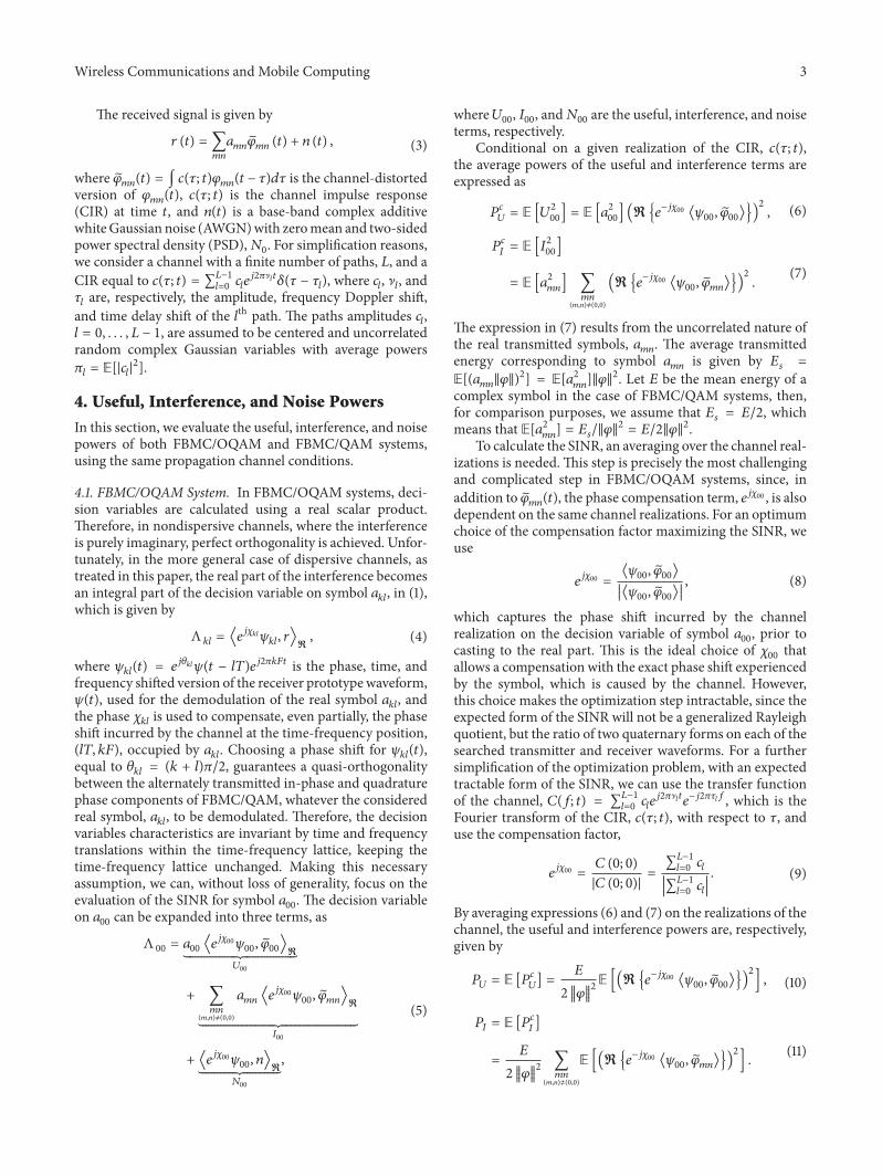
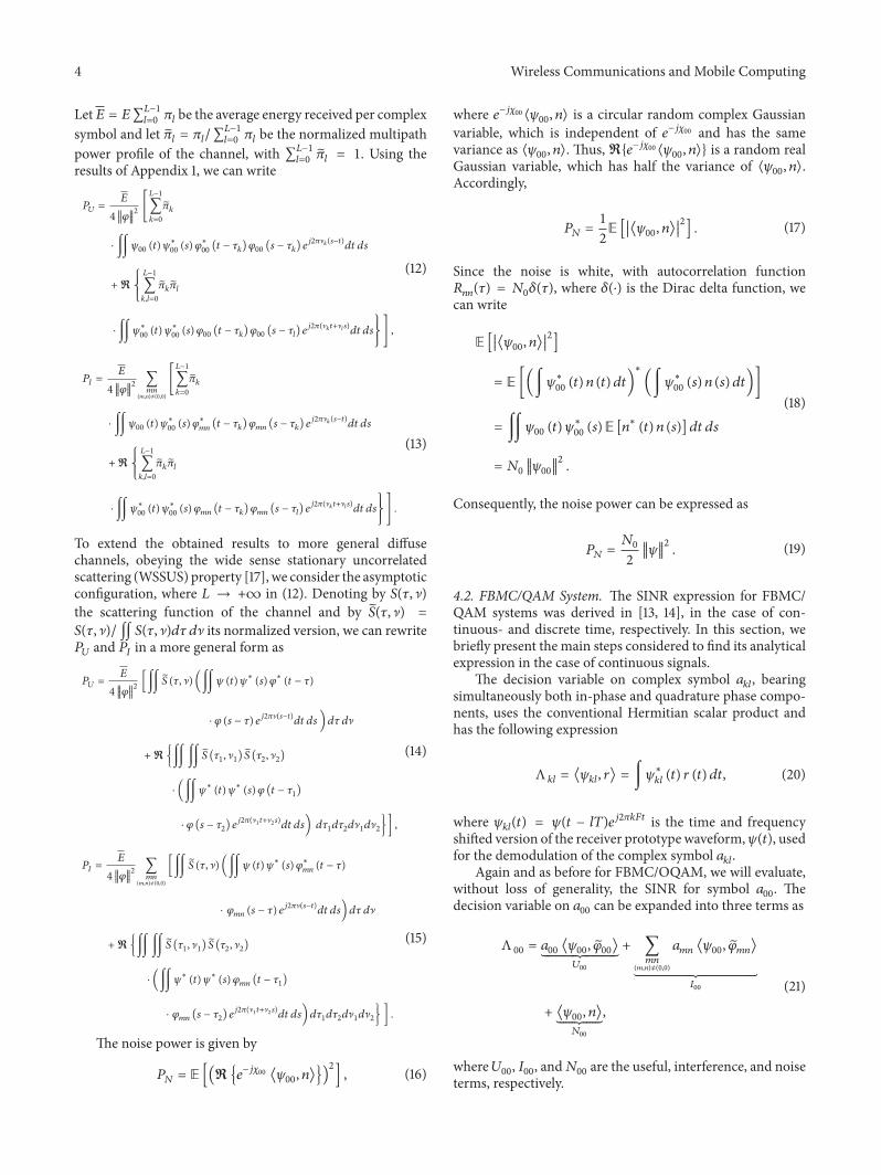
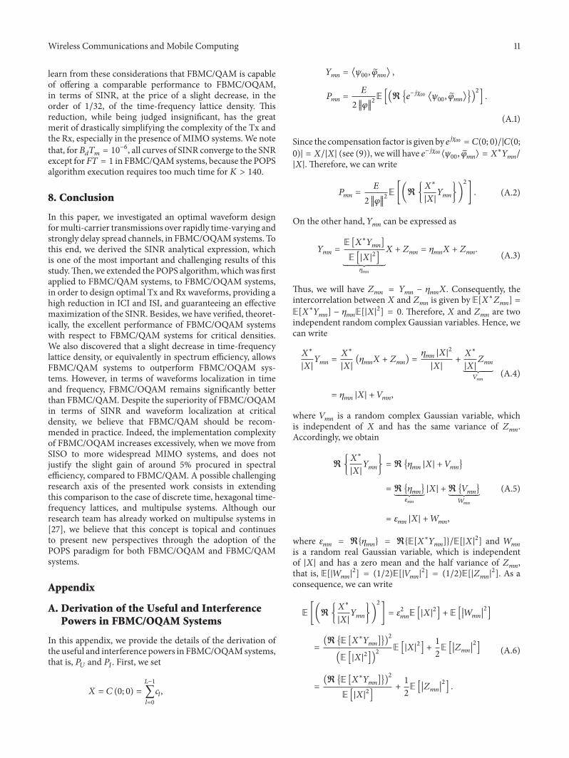

International Journal of
AerospaceEngineeringHindawiwwwhindawicom Volume 2018
RoboticsJournal of
Hindawiwwwhindawicom Volume 2018
Hindawiwwwhindawicom Volume 2018
Active and Passive Electronic Components
VLSI Design
Hindawiwwwhindawicom Volume 2018
Hindawiwwwhindawicom Volume 2018
Shock and Vibration
Hindawiwwwhindawicom Volume 2018
Civil EngineeringAdvances in
Acoustics and VibrationAdvances in
Hindawiwwwhindawicom Volume 2018
Hindawiwwwhindawicom Volume 2018
Electrical and Computer Engineering
Journal of
Advances inOptoElectronics
Hindawiwwwhindawicom
Volume 2018
Hindawi Publishing Corporation httpwwwhindawicom Volume 2013Hindawiwwwhindawicom
The Scientific World Journal
Volume 2018
Control Scienceand Engineering
Journal of
Hindawiwwwhindawicom Volume 2018
Hindawiwwwhindawicom
Journal ofEngineeringVolume 2018
SensorsJournal of
Hindawiwwwhindawicom Volume 2018
International Journal of
RotatingMachinery
Hindawiwwwhindawicom Volume 2018
Modelling ampSimulationin EngineeringHindawiwwwhindawicom Volume 2018
Hindawiwwwhindawicom Volume 2018
Chemical EngineeringInternational Journal of Antennas and
Propagation
International Journal of
Hindawiwwwhindawicom Volume 2018
Hindawiwwwhindawicom Volume 2018
Navigation and Observation
International Journal of
Hindawi
wwwhindawicom Volume 2018
Advances in
Multimedia
Submit your manuscripts atwwwhindawicom