How Much Do CEO Incentives Matter? ∗

Robert Tumarkin†

New York University

July 11, 2010

Abstract

The impact of CEO incentive compensation on firm performance is difficult to

quantify because performance also affects incentives. To circumvent this problem,

I form an estimate of the changes in CEO incentives caused by exogenous stock

price movements using a return index for each firm’s peer group and lagged CEO

holdings. For the mean incentive level, Tobin’s q increases by 10.0% compared to

that of counterfactual firms that lack CEO incentive compensation. I also introduce

an ex ante measure of the CEO’s discretion over her incentive portfolio and show

that the greater this discretion the less incentives mitigate agency conflicts.

∗The latest version of this paper can be download at http://www.stern.nyu.edu/~rtumarki/research/HMDCIM.pdf.†I thank my dissertation committee, Xavier Gabaix, Robert Whitelaw, and Jeffrey Wurgler, for their sup-

port and helpful discussions on this research. I also thank Justin Birru, Jennifer Carpenter, Alex Edmans,Farhang Farazmand, Xavier Giroud, Bryan Kelly, Yoel Krasny, William Greene, Matt Grennan, Jongsub Lee, HongLuo, Holger Mueller, Philipp Schnabl, Raghu Sundaram, Rik Sen, Stijn Van Nieuwerburgh, David Yermack, andMichelle Zemel for their constructive comments. This paper has benefited from seminar participants at BloombergL.P., Dartmouth College, University of Delaware, University of Michigan, Pennsylvania State University, New YorkUniversity, Notre Dame, University of New South Whales, and the U.S. Securities and Exchange Commission.Address: Leonard Stern School of Business, New York University, 44 West Fourth Street, New York, NY 10012.Email: robert.tumarkin@stern.nyu.edu Web: www.stern.nyu.edu/~rtumarki Phone: (212) 998-0313 Cell: (646) 450-7628

The empirical relationship between incentives and firm performance is a foundational

issue in corporate finance. Whether incentives actually create value has been a subject of

debate in the empirical literature. This paper quantifies how much incentives (positively)

impact firm value using an empirical approach that carefully addresses endogeneity between

incentives and performance. My results suggest an economically meaningful reduction in

agency conflicts from observed CEO incentive contracts. When firm performance is measured

by Tobin’s q, the ratio of firm value to replacement value, mean CEO incentives increase

firm value by 10.0% over counterfactual companies that lack CEO incentive compensation.

Moreover, I examine the efficacy of incentives under different CEO incentive-portfolio

structures. I introduce an intuitive, ex ante measure of the discretion the CEO has over

her private incentive portfolio through option-exercise policy and voluntary transactions in

company stock. The marginal value of incentives is inversely related to the amount of CEO

discretion.

The econometric challenge of quantifying the impact of CEO incentives on firm perfor-

mance is demonstrated by contradictory findings in the existing literature. Demsetz and

Lehn (1985) provide evidence against the Berle-Means thesis, showing instead that execu-

tives with small ownership stakes in firms do not have reduced incentives to maximize firm

profits. Morck, Shleifer, and Vishny (1988) directly investigate the role of management own-

ership in creating value. They find a non-monotonic relationship between ownership and

value.

Later papers confront the estimation issues that arise when ownership and performance

are endogenously determined. However, the results are established, to a degree, by the choice

of empirical model. Papers with fixed-effects panels find no link between management own-

ership and performance (Himmelberg, Hubbard, and Palia 1999, Palia 2001). Palia controls

for endogenous incentive levels through four instrumental variables: CEO experience, CEO

1

education quality, CEO age, and firm volatility. He finds no statistical relationship between

incentive compensation and firm value, suggesting that firms are in equilibrium when CEO

contracts are set. Countering this branch of research, Zhou (2001) contends that the relation-

ship between management ownership and performance can only be found in the cross-section.

Thus, fixed-effects models eliminate important cross-sectional variation and give the specious

result that ownership and performance are unrelated.

My empirical methodology provides an improved approach to identification over those

used previously. It addresses endogeneity between CEO incentives and firm performance,

while accounting for fixed effects. The approach emphasizes the importance of changes in

CEO incentives. CEOs are rewarded for good firm performance, whether from skill or luck

(Bertrand and Mullainathan 2001), so it is not possible to infer that incentives help firm

performance merely by observing that the two are positively correlated.

Successful identification requires isolating exogenous changes in CEO incentives. Incen-

tives are established through equity-linked securities. Therefore, by observing stock price

movements, it is possible to estimate changes in CEO incentives as a function of both the

structure of the incentive portfolio and stock returns. Unfortunately, if the market is forward

looking, stock returns may anticipate future performance innovations and estimated changes

will be endogenous. To combat this, for each CEO, I create an index of the stock returns of

her firm’s competitors. Multiplying the returns on this index by lagged information on the

CEO’s portfolio creates a instrument for changes in incentives.

Two identification assumptions are necessary for the instrument to be valid. First, I

assume that the CEO’s incentive portfolio does not predict firm performance innovations

indefinitely. I allow for incentives to predict firm performance innovations, perhaps due to

inside information. But, there is a finite period over which incentives are correlated with

performance innovations.

2

Second, I make the most of the panel structure of my data to isolate the exogenous

component of firm stock returns. I assign firms to economic groups and subgroups. I assume

that, after controlling for a time-varying group mean, firm specific performance shocks are

independent within subgroups. Given this assumption, a performance shock for a specific

firm will be independent of the excess stock return of a peer in the same subgroup. Returns of

firms within the subgroup will be correlated due to shared economic drivers and can be used

to compute an exogenous return index. This approach is similar to identification techniques

used in Hausman (1997) and Nevo (2001). In the main text, I assume that an economic

group’s average Tobin’s q changes each year, which is captured econometrically by dummy

variables for each group-sample year observation. I construct instruments using the returns

of a CEO’s competitor firms in the same economic subgroup.

The definitions of groups and subgroups are critical for valid identification. I use robust-

ness tests to ensure that the modeled structure of time-varying performance means does not

determine the results. Using a taxonomy that classifies firms, I run tests assuming the time-

varying means exist, in increasing specificity, at the sector, industry group, and industry

level. The instruments must be defined such that dummy-variables capturing time-varying

means do not weaken their identification power. Therefore, when computing return instru-

ments, I use a firm’s industry group peers when shocks to means are assumed to occur at the

sector level, industry peers when shocks to means are assumed to occur at the industry group

level, and sub-industry peers when shocks to means are assumed to occur at the industry

level.

Recent papers have examined the impact of incentives on firm value using alternate econo-

metric approaches. Fahlenbrach and Stulz (2009) regress large changes in Tobin’s q on

lagged changes in managerial ownership. Treating the lagged change in ownership as strictly

exogenous, Fahlenbrach and Stulz find that the elasticity of q with respect to ownership is

3

approximately one. While my empirical approach uses a similar difference-in-difference spec-

ification for estimation, I relax the assumption that changes in CEO incentives are strictly

exogenous from innovations in firm performance and provide instruments for changes in CEO

incentives.

Habib and Ljungqvist (2005) consider a large sample of U.S. firms. They employ stochas-

tic frontier analysis to derive the hypothetical maximum value for a firm. They find that the

average Tobin’s q is 16% below the optimal, which would be realized by first-best contract-

ing. In other research, Ang, Cole, and Lin (2000) examine firms that are 100% owned by

management. These firms, which do not have agency costs, are benchmarks against which

other companies are valued. However, since the benchmark firm is required, their study is

limited to small companies. Habib and Ljungqvist and Ang, Cole, and Lin measure the

distance between observed and optimal firm values. By contrast, my work is unconcerned

with finding the optimal firm value. Instead, I quantify the value created by incentives in

observed firms from counterfactual benchmark firms lacking incentive compensation. This

method identifies the average agency costs eliminated by incentives.

In a different context, Bettis, Bizjak, and Lemmon (2001) demonstrate that managers

of dual-purpose closed-end mutual funds behave in accordance with the incentives created

by separate income and capital-gains shares. They show that the market prices manager

behavior fostered by these contracts.

A discussion of the measure of incentives and identification follows in Section I. Section II

summarizes the data and reviews the choice of control variables. Estimation and the value

of CEO incentives are analyzed in Section III. Section IV quantifies how CEO discretion

significantly changes the value created by incentives. Robustness tests are contained in

Section V, and Section VI concludes.

4

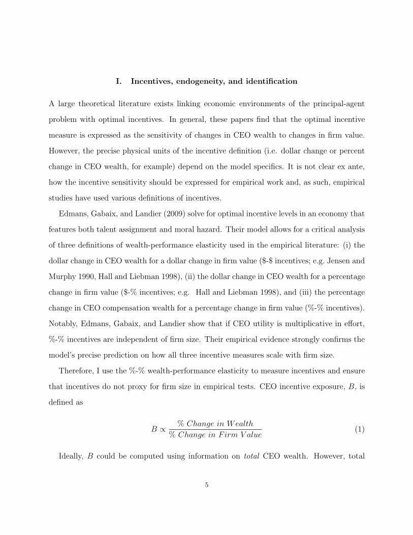
I. Incentives, endogeneity, and identification

A large theoretical literature exists linking economic environments of the principal-agent

problem with optimal incentives. In general, these papers find that the optimal incentive

measure is expressed as the sensitivity of changes in CEO wealth to changes in firm value.

However, the precise physical units of the incentive definition (i.e. dollar change or percent

change in CEO wealth, for example) depend on the model specifics. It is not clear ex ante,

how the incentive sensitivity should be expressed for empirical work and, as such, empirical

studies have used various definitions of incentives.

Edmans, Gabaix, and Landier (2009) solve for optimal incentive levels in an economy that

features both talent assignment and moral hazard. Their model allows for a critical analysis

of three definitions of wealth-performance elasticity used in the empirical literature: (i) the

dollar change in CEO wealth for a dollar change in firm value ($-$ incentives; e.g. Jensen and

Murphy 1990, Hall and Liebman 1998), (ii) the dollar change in CEO wealth for a percentage

change in firm value ($-% incentives; e.g. Hall and Liebman 1998), and (iii) the percentage

change in CEO compensation wealth for a percentage change in firm value (%-% incentives).

Notably, Edmans, Gabaix, and Landier show that if CEO utility is multiplicative in effort,

%-% incentives are independent of firm size. Their empirical evidence strongly confirms the

model’s precise prediction on how all three incentive measures scale with firm size.

Therefore, I use the %-% wealth-performance elasticity to measure incentives and ensure

that incentives do not proxy for firm size in empirical tests. CEO incentive exposure, B, is

defined as

B ∝ % Change in Wealth

% Change in F irm V alue(1)

Ideally, B could be computed using information on total CEO wealth. However, total

5

wealth is not observable in United States data. Only changes in incentive wealth may be

observed. These are estimated using the CEO’s holdings in performance-linked securities,

such as stock or stock options. Equation (1) implies that a feasible calculation in the data is

B =∆ $Wealth

$ Total Annual Compensation

1

∆ ln Firm V alue

=∆BS · S

$ Total Compensation(2)

where ∆BS is the total Black-Scholes Delta from option and stock exposure and S is the stock

price. The Black-Scholes Delta is the elasticity of the CEO’s incentive portfolio value to the

underlying stock price. Here, incentives are the dollar change in wealth, scaled by annual

total compensation, for a percentage change in firm value. Total annual compensation is

used as a proxy for scaling by total CEO wealth as in Edmans, Gabaix, and Landier and

stock returns are used to approximate change in firm value. The details of computing B are

discussed in Section II.

Per the existing literature (e.g. Core and Guay 2002), utility gains from human capital

or from expected future compensation are ignored in B. Research suggests that the primary

source of CEO incentives is from existing securities, not from future salary increases (Core,

Guay, and Verrecchia 2003, Hall and Liebman 1998). Hence, the approximation of changes

in total wealth by changes in incentive wealth should induce little error in the results.

A. Endogeneity and identification

Firm performance and CEO compensation are determined simultaneously. Bertrand and

Mullainathan (2001) show that CEOs are rewarded for shocks to performance, even random

shocks. Therefore, incentives and innovations in performance will be contemporaneously

correlated. Incentives may even anticipate performance innovations if, for example, the

board has inside information on an innovation to earnings at t + 1 and increases CEO

6

incentives at t. Such a possibility creates endogeneity between current incentives and future

performance innovations.

Identification requires finding an instrument for the level of CEO incentives. However,

level instruments, such as CEO characteristics, are cross-sectional and, therefore, may not

function well in panels that control for fixed-effects. Instead, I transform the level relationship

into an expression for the relation between changes in CEO incentives, ∆B, and changes

in firm performance for estimation. Doing so allows me to create a strong econometric

instrument and break endogeneity between CEO incentives and firm performance.

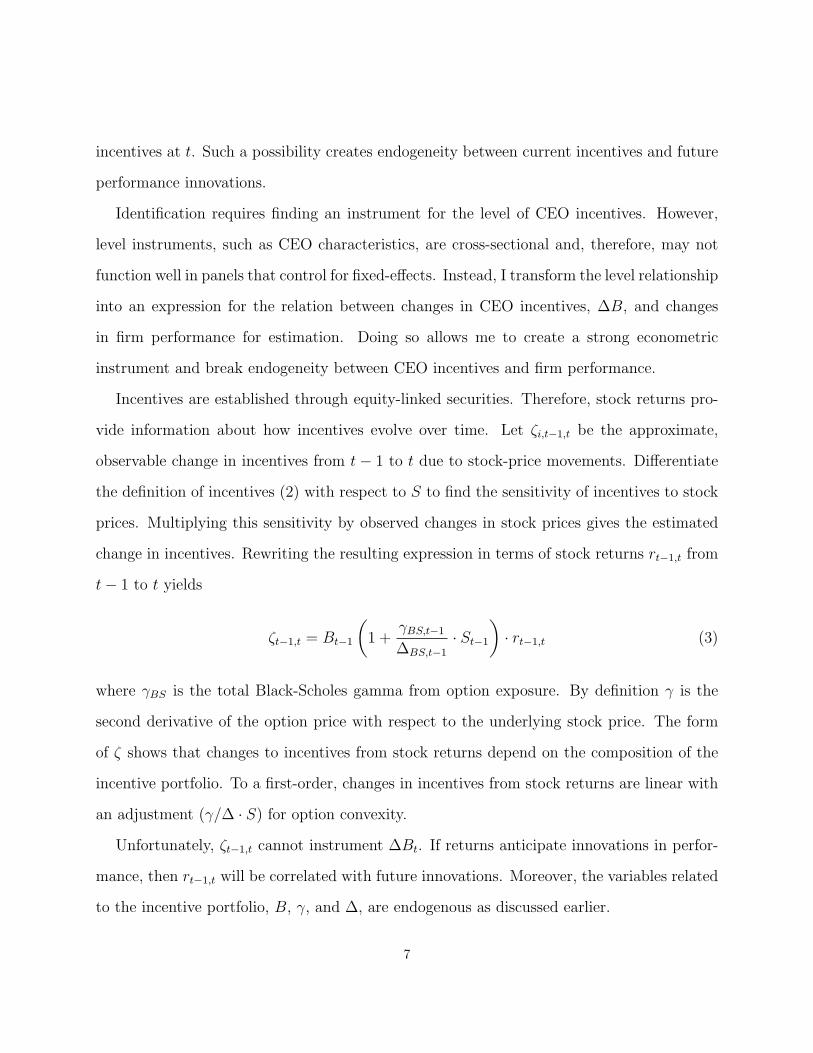
Incentives are established through equity-linked securities. Therefore, stock returns pro-

vide information about how incentives evolve over time. Let ζi,t−1,t be the approximate,

observable change in incentives from t− 1 to t due to stock-price movements. Differentiate

the definition of incentives (2) with respect to S to find the sensitivity of incentives to stock

prices. Multiplying this sensitivity by observed changes in stock prices gives the estimated

change in incentives. Rewriting the resulting expression in terms of stock returns rt−1,t from

t− 1 to t yields

ζt−1,t = Bt−1

(1 +

γBS,t−1

∆BS,t−1

· St−1

)· rt−1,t (3)

where γBS is the total Black-Scholes gamma from option exposure. By definition γ is the

second derivative of the option price with respect to the underlying stock price. The form

of ζ shows that changes to incentives from stock returns depend on the composition of the

incentive portfolio. To a first-order, changes in incentives from stock returns are linear with

an adjustment (γ/∆ · S) for option convexity.

Unfortunately, ζt−1,t cannot instrument ∆Bt. If returns anticipate innovations in perfor-

mance, then rt−1,t will be correlated with future innovations. Moreover, the variables related

to the incentive portfolio, B, γ, and ∆, are endogenous as discussed earlier.

7

It is possible to instrument ∆Bt if the exogenous change in CEO incentives is isolated.

To create such an instrument, two identification assumptions are necessary. First, I assume

that incentives at t− 2 are independent of the performance innovation at t. This will occur

in equilibrium, for example, if there is no inside information or inside information has a

one-year time horizon. Under this assumption, all variables that derive from incentive data

at time t−2, Bt−2, γt−2, and ∆t−2, will be independent of the time t performance innovation.

Second, I capitalize on the panel structure of my data and assign firms to economic groups

and subgroups. I assume that, after controlling for a time-varying group performance mean,

firm specific performance shocks are independent within subgroups. Given this assumption,

a performance shock for a specific firm will be independent of the stock return of a peer in

the same subgroup. Returns of firms within the subgroup will be correlated due to shared

economic drivers and can be used to compute instrumental variables. This approach is

similar to identification techniques used in Hausman (1997) and Nevo (2001).

Using the two assumptions above, I create an instrument for changes in CEO incentives.

For each firm, I identify companies in the same subgroup. These are firms in the sample

with the same business focus. Let r−it−1,t be the equally weighted average of these company

returns, excluding firm i, computed with monthly rebalancing. I use information about the

CEO’s portfolio at t − 2 to create a valid instrument for changes in CEO incentives. This

instrument Z is given by

Zt−1,t = Bt−2

(1 +

γt−2

∆t−2

· St−2

)· r−i

t−1,t (4)

The use of a first-order approximation for changes in incentives allows for a clear articu-

lation of the identification assumptions necessary to construct valid instruments. Alternate

computations for changes in incentives due to stock returns exist. For example, it is pos-

sible to compute changes in incentives using the definition of B, equation (2), evaluated

8

with data at two time observations. However, such a definition requires instrumenting the

Black-Scholes Delta formula, a highly non-linear function. By focusing on a first order ap-

proximation for changes in incentives, equation (3), it is easy to isolate the separate effects of

incentive levels and of stock returns on changes in incentives and, thereby, clearly articulate

the identification assumptions.

II. Data

The core information on CEO compensation structure is provided by Standard & Poor’s

Executive Compensation (Execucomp) Database. Only executives explicitly identified as

a CEO for a firm-year observation are used. Execucomp data is extracted from corporate

annual proxy statements (SEC Form DEF 14A). For the period studied, the proxy statement

provides data on new stock grants, outstanding stock grants, share ownership, and total

compensation for each CEO on an annual basis. The data on new stock and option grants

is comprehensive. Executives may receive multiple incentive grants in a year. For each,

Execucomp details the size of the grant, the strike price of the options, and the option

maturity. Data on existing executive options is limited. Until 2006, companies were only

required to break the existing options data into two groups, exercisable and non-exercisable.

For each group, two summary statistics are available: the number of outstanding options

and their intrinsic value. Beginning with 2006, reporting requirements were changed so that

companies must provide detailed information on all executive option positions. I use the

older, more opaque data format in order maximize the time frame of this study. Finally,

CEO stock-ownership information consists of the number of restricted and unrestricted shares

owned, excluding options.

Information on firm financial performance is taken from the Compustat North America

annual data file. All nominal variables are deflated using quarterly GDP deflators provided

9

by the Bureau of Economic Analysis. The Federal Reserve’s online data supplies risk-free

rates.

Economic group definitions are per GICS as provided through Compustat. In increasing

degree of specificity, each company is categorized by sector, industry group, industry, and

subindustry. Occasionally, the classification of a company may switch for a year and then

return to the original classification. This is corrected as necessary.

The Corporate Library lists the years that firms in the sample were founded. This data

is extracted from SEC proxy statements whenever possible. If necessary, The Corporate

Library uses company websites as a secondary source for firm founding data. Founding year

is available for approximately 80% of the firms in the sample. For the remaining companies,

manual review of each firm’s proxy statement was necessary to determine the founding year.

Finally, the Center for Research in Security Prices (CRSP) daily database is used for

stock returns. The CRSP/Compustat Merged Database (CCM) supplies the link between

Compustat’s gvkey identifier and CRSP’s permno.

A. Sample selection

I begin with all CEO-year observations from Execucomp for firms with fiscal years ending

from 1994 through 2006. The observations that do not have matching CRSP and Compustat

North America data are removed. I eliminate Financial Services and Utility companies

from the empirical analysis. These two industries are heavily regulated, which may lead to

incentives having a very different role than in other industries. The elimination of Financial

Services and Utilities follows the procedure of recent researchers (see, for example, Coles,

Daniel, and Naveen 2006, Lewellen 2006, Low 2009).

Baker and Hall (2004) argue that founder CEOs are simultaneously principals and agents

of their firms. Given this, their incentive packages may differ in systematic ways from those

10

of professional managers at established firms. I adapt the method used by Adams, Almeida,

and Ferreira (2009) and define founder CEOs as those CEOs that joined a firm less than 4

years after the date of incorporation. Founders account for approximately 31% of the sample

and are removed from the analysis.

Due to the empirical approach and instrumentation technique, the data requirement for

estimation depends on the empirical specification. A maximum of 5,011 and a minimum of

4,110 observations are used in the tests. Each observation includes firm performance at time

t+ 1 and incentive and control variables at time t.

Incentive levels are computed for each CEO on an annual basis. The key input is the

Black-Scholes Delta ∆BS of the executive’s portfolio. For any financial security, Delta is

defined as the dollar change in the security’s value for a dollar change in the underlying

stock. The executive’s portfolio Delta is found by adding up the Deltas of each security held

in her compensation portfolio. See Appendix B for details on how Delta is computed.

In order to compute %-% incentives B for each CEO-fiscal year observation, Edmans,

Gabaix, and Landier (2009) use total annual compensation as a proxy for total CEO wealth.

However, established CEOs may receive low total compensation in a year, but have large

existing stock and option holdings. In such a case, total compensation does not accurately

represent wealth. For example, in the data, scaling by total annual compensation yields a

median incentive of ten but a maximum of two billion.

Instead, I use a CEO compensation value fitted from cross-sectional analysis to scale

total portfolio Delta. Doing so reduces the influence of outliers and provides an alternate

proxy for wealth than actual CEO compensation. Compensation includes salary, cash bonus,

stock and option awards, and other forms of remuneration. Edmans, Gabaix, and Landier

(2009) predict that compensation is also subject to a hidden reference firm size. I use the

cross-section of total compensation to derive a fitted compensation level for each CEO-year

11

observation. Specifically, I estimate the regression

log(Compensationi,t) = at + b · log(Total F irm V aluei,t−1) + εi,t (5)

where the time fixed-effect at captures the hidden reference firm size. Edmans, Gabaix, and

Landier (2009) predict that log compensation scales at a rate of 1/3 to log firm value. In my

data, b has a point estimate of 0.391 and a robust standard error of 0.083. Therefore, the

coefficient from the regression conforms to the empirical prediction of Edmans, Gabaix, and

Landier (2009).

I use the fitted compensation values implied from regression equation (5), CompensationFittedi,t ,

to scale Delta exposure and define %-% incentives

B =∆BS

S · CompensationFitted(6)

where ∆BS is the total Black-Scholes Delta of the portfolio and S is the underlying stock

price.

Execucomp collects the incentive portfolio data from each company’s annual proxy state-

ment (DEF14A). Option ownership details are as of fiscal year end. However, share ownership

is reported as of a day between the fiscal year end and the filing of the proxy statement, which

may be filed up to 120 days after fiscal year end. Therefore, the incentive measure combines

two distinct observation times for each CEO-year in the sample. Since an observation on

the total level of incentives for a fiscal year includes up to four months of information about

the executive’s portfolio evolution in the next fiscal year, time-t incentives are endogenous

to both t and t+ 1. This is addressed appropriately during estimation.

12

B. Model selection

Optimal contracting through incentive compensation exists to reduce agency costs. There-

fore, the benefit of incentives should be seen directly in improved firm performance. I examine

both a market-based measure as well as an accounting measure of firm performance in or-

der to provide a robust analysis of the function of CEO incentives. If markets are efficient,

then the impact of incentives should be seen in firm market value. I focus on firm value as

characterized by Tobin’s q, defined as the ratio of the firm’s market value to the replacement

cost of its assets. For the accounting metric, I use earnings before interest and taxes nor-

malized by the start of year book value of assets (EBIT-to-assets). Earnings are commonly

used to examine firm performance by many finance researchers and practitioners. While

they may be subject to manipulation from accruals (e.g. Bergstresser and Philippon 2006),

Dechow (1994) shows that earnings are a better measure of performance than cash flows

over short-time intervals. Alternate accounting metrics, including earnings before interest,

taxes, depreciation, and amortization (EBITDA), return on assets, net profit margin, and

market-to-book ratio, exhibit qualitatively similar relationships with CEO incentives.

To control for firm performance, I follow the guidelines established by Habib and Ljungqvist

(2005) and Himmelberg, Hubbard, and Palia (1999) in choosing control variables. These

controls derive from a large literature on the determinants of Tobin’s q. As value exhibits

diminishing returns to scale, Tobin’s q should decrease as firm size increases. Firms with

better growth opportunities and that are more efficient or profitable should have a higher

Tobin’s q. If there is a tax benefit to debt, leverage should be associated with value. Fi-

nally, Habib and Ljungqvist (2005) argue that the relative importance of tangible capital

to the firm can influence q. These controls are also used for EBIT-to-assets. Additionally,

when appropriate, lagged performance values are used to capture the dynamic process of

performance.

13

The specific variables used as controls follow. I use the log of total net sales as a measure

of firm size. Growth opportunities are captured by research and development (R&D) in-

tensity, capital expenditure intensity, acquisition intensity, and year-over-year sales growth.

Operating margin scaled by sales is my measure for profitability. Finally, I use the capital-

to-sales ratio to account for tangible capital. Precise definitions of all variables, as well as

the fields for computing them within Compustat, are listed in Table I.

My empirical specification allows for time-varying, industry-level dummy variables. Hence,

the industry level controls of Habib and Ljungqvist (2005), such as growth forecasts and the

cost of capital, are not necessary here. Tests in Section V show that the results are robust

to different industry specifications.

C. Descriptive statistics

Table II presents descriptive statistics for the sample. All dollar values are expressed in real

terms, as of the year 2000. In order to limit the impact of outliers on the panel results

presented later, all variables are winsorized at the 1% and 99% levels.

CEOs in the sample earn $4.4 million on average in total compensation, which includes

salary, bonus, option grants, restricted stock grants, and other forms of payment. The typical

CEO is experienced, with an average tenure of 6.4 years and an average age of 56.1 years.

CEO incentive portfolio wealth is sensitive to firm performance for the period covered by

the sample. The average CEO has %-% incentives B of 20.4. Thus, a 1% increase in firm

value results in the average CEO wealth increasing by 20.4% of annual salary. The median

B is 8.7, indicating the distribution of incentives is skewed. Some CEOs have a large amount

of their wealth tightly tied to firm performance.

The firms in the sample have an average value to replacement cost, Tobin’s q, of 2.04.

EBIT-to-asset ratio is, on average, equal to 11.4%.

14

Finally, the firms in the sample expend on average 10% of their assets on capital ex-

penditures annually. While the average spending is 3% and 4% of assets each for R&D

and acquisitions, respectively, the median firms engage in neither research and development

nor acquisitions. Thus, acquisitive firms and firms with high research budgets represent a

minority in the sample.

III. The average value of CEO incentives

Consider a model of the relationship between current levels of CEO incentives, B, and future

firm performance, y, in a simple predictive regression. Bertrand and Schoar (2003) show that

CEO fixed-effects account for significant differences in investment and financing practices

across firms. Moreover, manager fixed-effects are correlated with compensation. Therefore,

to control for both firm and CEO fixed-effects, the empirical model must be structured by

CEO-firm observations.

Firm performance may be dynamic. That is, current performance may be a function of

past performance. Let Xi,t be a vector of control variables for performance for CEO-firm i

at time t. Then the performance process for CEO-firm i in economic group j may be written

yi,t+1 = αyi,t + βBi,t + γXi,t + ηi + φj,t+1 + εi,t+1 (7)

where α allows for a dynamic performance process, ηi is a fixed effect for CEO-firm combi-

nation i, φj,t+1 is a time varying group mean common to all firms in economic group j, and

εi,t+1 is an idiosyncratic innovation to performance.

As discussed in Section I, I assume that after controlling for a time-varying group per-

formance mean, firm specific performance shocks are independent within subgroups. The

group performance mean, φj,t+1, is thus a critical component in the identification strategy.

In this section, I assign firms to one of 8 economic sector groups. For each group, the mean

15

performance changes each fiscal-year. Return instruments are computed using 19 industry

peer groups.

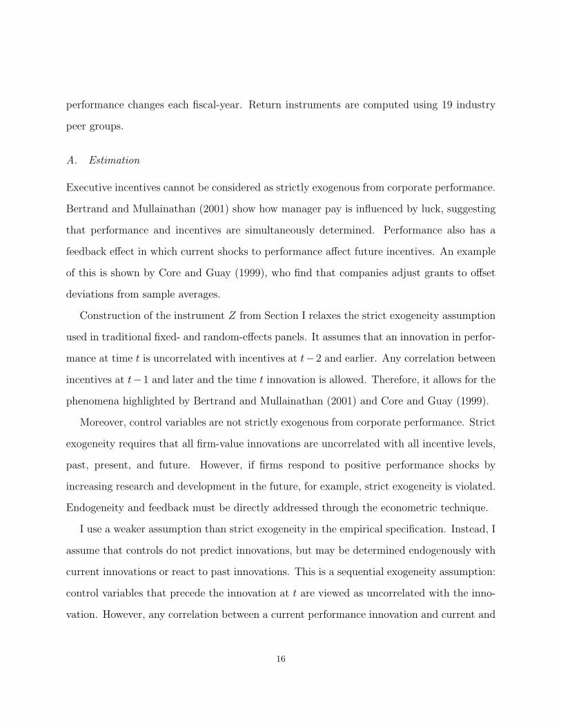
A. Estimation

Executive incentives cannot be considered as strictly exogenous from corporate performance.

Bertrand and Mullainathan (2001) show how manager pay is influenced by luck, suggesting

that performance and incentives are simultaneously determined. Performance also has a

feedback effect in which current shocks to performance affect future incentives. An example

of this is shown by Core and Guay (1999), who find that companies adjust grants to offset

deviations from sample averages.

Construction of the instrument Z from Section I relaxes the strict exogeneity assumption

used in traditional fixed- and random-effects panels. It assumes that an innovation in perfor-

mance at time t is uncorrelated with incentives at t−2 and earlier. Any correlation between

incentives at t−1 and later and the time t innovation is allowed. Therefore, it allows for the

phenomena highlighted by Bertrand and Mullainathan (2001) and Core and Guay (1999).

Moreover, control variables are not strictly exogenous from corporate performance. Strict

exogeneity requires that all firm-value innovations are uncorrelated with all incentive levels,

past, present, and future. However, if firms respond to positive performance shocks by

increasing research and development in the future, for example, strict exogeneity is violated.

Endogeneity and feedback must be directly addressed through the econometric technique.

I use a weaker assumption than strict exogeneity in the empirical specification. Instead, I

assume that controls do not predict innovations, but may be determined endogenously with

current innovations or react to past innovations. This is a sequential exogeneity assumption:

control variables that precede the innovation at t are viewed as uncorrelated with the inno-

vation. However, any correlation between a current performance innovation and current and

16

future values of the control variables is allowed. Sequential exogeneity is a weaker assumption

than the strict exogeneity assumption required by random- and fixed-effects panels.

Estimation of equation (7) begins by removing the fixed effect ηi using a first-difference

transformation. The first differenced performance process is

∆yi,t+1 = α∆yi,t + β∆Bi,t + γ∆Xi,t + ∆φj,t+1 + ∆εi,t+1 (8)

Estimation proceeds using two-step efficient GMM. Changes in incentives, ∆Bi,t, are in-

strumented by contemporaneous changes computed using the instrument Z as described in

Section I. This breaks endogeneity and identifies the economic coefficient relating incentives

and firm performance, β in equation (8). All control variables are treated as endogenous;

lagged levels instrument first differences during estimation. If sequential exogeneity assump-

tions are satisfied, these level instruments identify the remaining coefficients. The precise

moment condition definitions are detailed as assumptions (13) and (14) in Appendix A.

This approach, due to Arellano and Bond (1991), addresses problems caused by endo-

geneous variables and feedback. Since lagged levels are used as instruments in a GMM

framework, innovations to performance influencing current and future incentives and other

controls does not bias estimation. By contrast, panel data methods, such as traditional

random- and fixed-effects models, necessarily assume strict exogeneity. If performance inno-

vations systematically influence future incentive levels, estimation will be biased. This bias

will not disappear even with large cross-sections. Arellano and Bond estimation allows for

consistent estimation of panels under sequential exogeneity like the one studied here, which

have short time frames but a large number of cross-section units.

To illustrate the method, consider empirical specification (8). After first differencing, the

equation for estimation contains the innovation term (εi,t+1 − εi,t). Provided that the basic

error ε is serially uncorrelated, then, under sequential exogeneity, all right-hand-side level

17

variables up through t−1 are uncorrelated with the differenced error. If ε exhibits first-order

serial correlation, then right-hand-side variables prior to and including t−2 are uncorrelated.

These facts allow for the construction of a sufficient number of moment conditions in which

level variables are used as instruments for the differenced variables in the estimation equation.

The critical assumption on the order of serial correlation in ε is tested empirically. Under

the assumption of serially uncorrelated errors ε, first differenced errors should not display

second-order serial correlation. The M2 test evaluates a null of no second-order serial correla-

tion in first-differenced errors. When it rejects the null, ε exhibits first-order serial correlation

and the sequential exogeneity moment conditions are adjusted as described earlier. The M3

is used to verify a null in which the non-differenced errors have first-order serial correlation,

in which case differenced errors should not exhibit third-order serial correlation. Reported

standard errors are robust to the observed serial correlation and heteroskedasticity. Standard

errors also include the finite sample correction documented in Windmeijer (2005).

I use a J-test of over-identifying restrictions to test the model. The sequential exogeneity

assumption allows for instrumentation of any first differenced variable with preceding level

variables. Therefore, the number of instruments available is factorial in the time dimension

and there are a large number of over-identifying moment conditions. But, if too many

instruments are used in estimation, the J-test has extremely low power (Bowsher 2002,

Roodman and Floor 2009). In fact, Bowsher (2002) shows that the full instrument set will

neither reject the null nor relevant alternatives. In order to limit the number of instruments,

I use no more than three lagged levels of a variable as instruments during estimation.

In general, effective estimation with Arellano and Bond (1991) requires that lagged levels

of a variable are good instruments for first differences. Since incentives are persistent, lagged

levels are poor instruments for changes in B. Existing solutions to the problems raised by

persistent incentive levels are not applicable in this setting. Ahn and Schmidt (1995) and

18

Blundell and Bond (1998) provide additional moment restrictions, which require that the

deviation of the initial observation of incentives from the steady state incentive value is

uncorrelated with the fixed effect. However, the initial observation of incentives represents

a new CEO. A new CEO may be willing to accept a initial incentive level below the steady

state value in order to price themselves attractively for a high quality firm. Similarly, a CEO

looking at a bad firm may look for compensation above the steady state value in order to

accept the risk of joining a poorly performing company. Hsiao, Pesaran, and Tahmiscioglu

(2002) provides a MLE estimator that assumes homoskedastic normality of the innovation

process. Han and Phillips (2009) provides a GMM method which assumes white noise

errors. However, the current panel exhibits significant heteroskedasticity in the data across

time and the cross-section. Thus, these approaches can not be applied to the context of firm

performance and CEO incentives. Thus, the instrument Z from Section I is essential for

effective estimation.

B. Panel results

The full specification for performance (7), including control variables, is

yi,t+1 =αyi,t + βBi,t + δ1 log(Salest) + δ2AcquisitionIntensity + δ3CapexIntensity +

δ4R&DIntensityt + δ5Book Leveraget + δ6Operating Margint +

δ7Tangible Capitalt + δ8Sales Growtht + ηi + φj,t+1 + εi,t+1 (9)

As not all performance processes are necessarily dynamic, I impose a layer of model selection

during estimation for each measure of firm performance. For each process, I first evaluate

the unrestricted dynamic specification, equation (9). If α is not statistically significant, I

estimate a restricted static model with α = 0.

Table III presents results of estimating the relationship between incentives and perfor-

19

mance, equation (9), with annual fixed-effects for each of eight industry groups to capture

time-varying average industry performance. Columns (1) and (2) report results for Tobin’s

q. The estimated processes for EBIT-to-assets are shown in columns (3) and (4). Columns

(2) and (4) use the full set of controls. The form of the specifications in Table III repre-

sent the outcome from model selection. Tobin’s q does not have a statistically meaningful

relationship with lagged values after controlling for a time-varying annual industry group

mean performance, so the process is modeled as non-dynamic. On the other hand, EBIT-

to-assets is clearly a dynamic process. The coefficient on lagged earnings is significant, with

a z-statistic over 3.

Corporate performance, as measured by Tobin’s q and EBIT-to-assets, is improved by

incentives, as predicted by traditional contracting theory. Tobin’s q shows a strong positive

statistical relationship with incentives at greater than 99% confidence (z-statistic of 3.32)

when the full set of controls is used. Earnings has a meaningful association with incentives,

with confidence greater than 90% and a z-statistic of 1.98, when the full set of controls is

included in the predictive regression.

Controls enter the regressions as expected. Log sales proxy for firm size and diminishing

returns to scale. Increased sales are associated with lower Tobin’s q and lower EBIT-to-

assets. R&D is positively associated with Tobin’s q, suggesting that it captures growth

opportunities valued by the market, while R&D expenses directly reduce earnings as seen in

the results.

The M2 test for Tobin’s q does not reject the null of serially uncorrelated errors. Addi-

tionally, the specifications with and without controls both pass the J-test of over-identifying

restrictions. The specification with all controls generates p-values of 0.785 and 0.204 for the

M2 and J-test, respectively. EBIT-to-assets shows first-order serial correlation of errors in

the specification without control variables. As such, the moment conditions for estimation

20

are adjusted. The reestimated process does not reject a null of second-order serially uncor-

related errors in performance levels. Both specifications for earnings pass the J-test with

p-values of 0.640 and 0.388 for the specifications without and with controls, respectively.

C. How much CEO incentives matter

Executive incentives exist to mitigate agency conflicts. I define the value of incentives against

a counterfactual benchmark in which executives have no incentive exposure. This counter-

factual assumes that the executive is compensated with a fixed salary, thereby maximizing

agency costs. The value of incentives then represents the amount of agency costs eliminated

by second-best contracting.

By the definition above, the value of incentives is simply β×B for a given incentive level

B. The distribution of incentive levels is skewed as shown in Table II. I use the mean and

median values in the sample, B = 20.4 and B = 8.7, as reasonable incentive levels for a

CEO.

Table IV shows that incentives have an economically meaningful role in improving firm

performance. Average incentive levels make a significant impact, increasing Tobin’s q by

0.204, which is a 10.0% improvement in the mean level. For the median incentive level,

Tobin’s q increases by 4.3% of the mean level. Accounting performance as measured by

EBIT-to-assets also improves from incentives. The EBIT-to-assets ratio increases by 0.0063

for the mean incentive level, which is a 5.5% increase relative to the mean EBIT-to-assets

ratio.

IV. When are incentives most effective?

CEOs are given large amounts of discretion over firm strategy, their level of effort, and

incentives. If markets are efficient and information is perfect, stocks are priced correctly and

21

a rational CEO would never choose to hold stock in her company beyond that specified by a

contract. However, empirical evidence indicates that a vast majority of CEOs choose to hold

stock in their company above contracted minimums. Core and Larcker (2002) document

that CEOs often have explicit “target ownership plans,” encouraging them to hold stock in

addition to restricted shares. They find that only 7% of CEOs hold fewer securities than

this minimum level.

Observed incentive contracts give executives direct control over their exposure to firm risk

through option exercise policy and voluntary stock transactions. Executives may neutralize

changes to company-mandated incentives by adjusting their private portfolios. Alternatively,

they may add to their firm risk by purchasing stock. The empirical evidence supporting

both activities is strong. Ofek and Yermack (2000) show that executives trade in their

personal accounts to hedge new incentive grants. Malmendier and Tate (2005) document

that overconfident CEOs repeatedly purchase company stock.

To understand the role of CEO discretion intuitively, consider a CEO with expectations

of company stock returns that differ from that of the firm principals and the market. Such a

CEO may hold stock voluntarily. However, if stock prices increase, the executive can take a

variety of actions. Under a behavioral framework, she may view the price increase as market

confirmation of her strategic choices and effort level. If she holds onto her shares, effort

may not change. Alternatively, consider a rational framework for a CEO with expectations

identical to that of the market over company stock. If stock-price changes do not affect the

CEO’s outlook, then she will hedge changes to incentive levels. By hedging incentives, effort

stays constant. Under both scenarios, an increase in stock price does not automatically lead

to greater incentives and higher effort as predicted by standard agency theory.

In traditional contracting frameworks, incentives exist to drive CEO effort. A CEO

with discretion over her private portfolio changes the implication of traditional contracting.

22

Observed incentives represent a equilibrium level jointly determined by principal and agent.

Thus, the marginal value of incentives for CEOs with discretion over their portfolios may

not be equal to those of CEOs that do not.

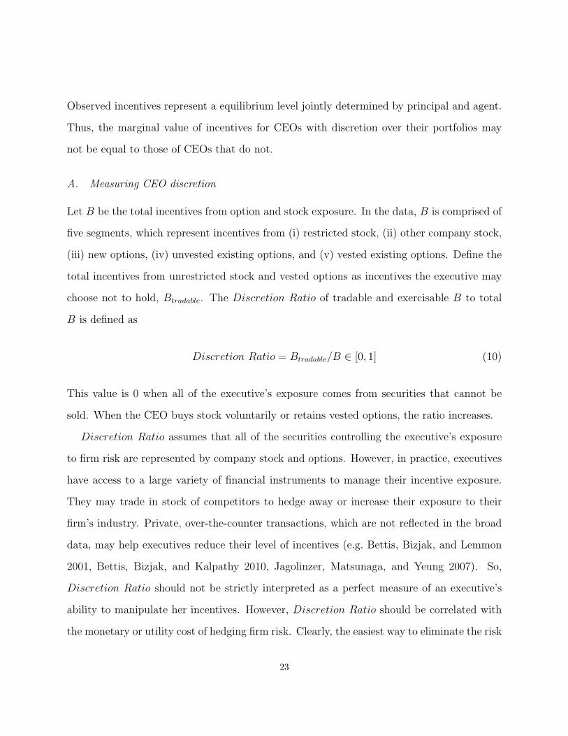
A. Measuring CEO discretion

Let B be the total incentives from option and stock exposure. In the data, B is comprised of

five segments, which represent incentives from (i) restricted stock, (ii) other company stock,

(iii) new options, (iv) unvested existing options, and (v) vested existing options. Define the

total incentives from unrestricted stock and vested options as incentives the executive may

choose not to hold, Btradable. The Discretion Ratio of tradable and exercisable B to total

B is defined as

Discretion Ratio = Btradable/B ∈ [0, 1] (10)

This value is 0 when all of the executive’s exposure comes from securities that cannot be

sold. When the CEO buys stock voluntarily or retains vested options, the ratio increases.

Discretion Ratio assumes that all of the securities controlling the executive’s exposure

to firm risk are represented by company stock and options. However, in practice, executives

have access to a large variety of financial instruments to manage their incentive exposure.

They may trade in stock of competitors to hedge away or increase their exposure to their

firm’s industry. Private, over-the-counter transactions, which are not reflected in the broad

data, may help executives reduce their level of incentives (e.g. Bettis, Bizjak, and Lemmon

2001, Bettis, Bizjak, and Kalpathy 2010, Jagolinzer, Matsunaga, and Yeung 2007). So,

Discretion Ratio should not be strictly interpreted as a perfect measure of an executive’s

ability to manipulate her incentives. However, Discretion Ratio should be correlated with

the monetary or utility cost of hedging firm risk. Clearly, the easiest way to eliminate the risk

23

from incentive securities is to sell stock or exercise options. These transactions are a perfect

hedge and can be executed instantaneously, subject to blackout periods and insider-trading

regulations. Private transactions, on the other hand, may be slow and costly. Trading in

competitors, on the other hand, while reducing industry risk, may increase idiosyncratic risk.

Discretion Ratio draws on the empirical evidence that executives actively manage their

level of incentives (Ofek and Yermack 2000). It is similar in spirit to a measure of managerial

overconfidence proposed by Malmendier and Tate (2005). Malmendier and Tate adapt the

option-exercise framework of Hall and Murphy (2002) to define overconfident managers as

those that do not exercise options with five years remaining even if the stock-price is 67%

above the strike price. The portfolio discretion measure in this paper also measures the

degree to which executives hold securities that could be sold or exercised. However, the

two measures have different objectives. Malmendier and Tate use a calibrated model to find

overconfidence. Here, I use a measure that adjusts for each security’s value to stock price

sensitivity. This correlates with portfolio flexibility, but not necessarily overconfidence. For

example, a manager by my definition could have maximal portfolio discretion by holding

vested at-the-money options. Such an executive would not be classified as overconfident by

Malmendier and Tate.

B. The CEO’s role

Under the hypothesis that CEOs have discretion over setting incentive levels, it is necessary to

modify the empirical process for firm performance, equation (9). I interact Discretion Ratio

with the level of incentives and include the variable separately as a control.

24

The revised specification for performance is

yi,t+1 =αyi,t + βBi,t + βDBi,t−1 ·Discretion Ratio + δ0Discretion Ratio +

δ1 log(Salest) + δ2AcquisitionIntensity + δ3CapexIntensity +

δ4R&DIntensityt + δ5Book Leveraget + δ6Operating Margint +

δ7Tangible Capitalt + δ8Sales Growtht + ηi + φj,t+1 + εi,t+1 (11)

If manager discretion reduces the efficacy of incentives, then the coefficient βD will be nega-

tive and significant. More complicated specifications, such as one in which Discretion Ratio

is interacted with all variables, yield similar results and are omitted for clarity of exposition.

Table V, columns (1) and (2) report the relationship between incentives and Tobin’s q.

Columns (3) and (4) present the process for EBIT-to-assets ratio. As before, I first estimate

an unrestricted dynamic model and then choose between that and a static one.

Manager discretion significantly reduces the ability of CEO incentives to create value.

Tobin’s q shows a positive relationship between incentives and firm performance, with 99%

confidence in specifications with and without controls. Importantly, the coefficient on B ·

Discretion Ratio is negative, also with greater than 99% confidence. Discretion Ratio

lies between 0 and 1 by construction. Therefore, the results indicate that the incentive-

performance elasticity for managers with full discretion would be about 72% lower than that

for managers with no discretion.

Specifications (1) and (2) have significantly different point estimates for the elasticities of

incentives on Tobin’s q and incentives interacted with discretion on Tobin’s q. However, the

implied economic impact of these elasticities is small, suggesting little cause for concern. The

mean Discretion Ratio in the sample is 0.70. Therefore, the average effective elasticity of

incentives and discretion for specification (1) is 3.48 (x1000), while the corresponding value

25

for specification (2) is 2.07 (x1000), which is calculated as the elasticity of incentives and

performance plus 0.70 times the elasticity of incentives, discretion, and performance.

The influence of CEO discretion on EBIT-to-assets is similar to that of Tobin’s q. In

the specification with controls, incentives reduce agency costs and improve earnings with

95% confidence. The impact of discretion is economically material. Incentives for CEOs

with full discretion are about 70% less effective at improving EBIT-to-assets than equivalent

incentives for managers with no discretion. This result has a z-statistic of 1.60.

The innovation processes for Tobin’s q pass theM2 test. The specifications with the full set

of controls fails to reject the null of non-serially correlated errors with a p-value of 0.663. Both

specifications for EBIT-to-assets do not exhibit first order serially correlated innovations.

The p-value with the full set of controls is 0.131. Additionally, both specifications for Tobin’s

q pass the J-test of over-identifying restriction with 95% confidence. Specifications (3) and

(4), the process for EBIT-to-assets, easily pass the over-identifying restrictions test, with

p-values of 0.825 and 0.938, respectively.

C. How much CEO incentives matter with CEO discretion

Table VI provides economic value for incentives when CEO discretion is included. Calcula-

tions proceed per the methodology used earlier to find the average value of incentives. I use

the average and median incentive levels. This value is interacted with quartiles of observed

Discretion Ratio values, 0.56, 0.74, and 0.89 for the 25th percentile, median, and 75th per-

centile, respectively. Note that the average Discertion Ratio is 0.70, not materially different

from the median value.

Analyzing the impact of mean incentive levels, B = 20.4, on Tobin’s q shows that when

CEO incentive portfolio discretion is relatively low (Discretion Ratio at the 25th percentile),

incentives are very effective. Tobin’s q increases by 0.303, which is a 14.8% change relative

26

to the mean level. As CEO discretion increases, the effectiveness of incentives declines signif-

icantly. For the median Discretion Ratio, Tobin’s q increases by 0.237 (11.6% of the sample

mean). Therefore, by moving from the 25th percentile to the median of Discretion Ratio, the

value of incentives on firm value is reduced by about 22%. For high Discretion Ratio, CEO

behavior removes about 41% of the marginal value of incentives. The increase in Tobin’s q is

0.180, or 8.8% of the mean. The impact of CEO discretion on EBIT-to-assets economically

resembles that for Tobin’s q.

V. Robustness tests

A. Alternate group mean specifications

As discussed in Section I, the instrument for changes in incentives may be invalid if there is a

common factor driving firm returns and the return index of competitors. In the main empiri-

cal specification, I allow for eight time-varying industry factors. However, if endogenous firm

performance shocks occur in industry groups, for example, then the model is misspecified.

I perform robustness tests to account for the possibility of more precise time-varying

economic cluster means. I use two different specifications: 19 time-varying economic group

and 64 time-varying industry means. As before, these are modeled empirically using dummy

variables for each category-year observation

Table VII shows results using the main empirical specification, equation (9). Columns

(1) and (2) of Table VII show robustness tests when each of 19 economic groups has a

unique, time-varying common factor. The results are robust to economic group-year factors.

Focusing on the specification with the full set of controls, incentives still have a positive

influence on firm value, with a t-stat of 2.36. Accounting for 64 industries in columns (3) and

(4) yields similar results, with a t-stat of 1.97. Economically, the results in columns (2) and

(4), the full set of control variables, suggest about a 30% reduction in economic magnitude

27

over the baseline estimates of Table IV. That is, the average incentive level increases firm

value by approximately 7% of average Tobin’s q.

B. Fama-French excess return instruments

Raw returns of peers are used to compute the instrument Z. It is possible that even after

accounting for sector, group, and industry time-varying means, the raw returns of peers are

still correlated with a firm’s idiosyncratic innovation. Estimation would then be biased.

An alternate way to define the instrument Z is to use the average excess return of peers

in equation (4) instead of the average raw return of peers. To do so, I use a Fama-French

three-factor model to calculate excess returns (Fama and French 1993). The average of

these excess returns for each firm’s peer group is used to compute the alternate instrument.

Empirical tests with this instrument yield results shown in Table VIII, which have similar

economic magnitudes and statistical significance to those from main specification.

VI. Conclusion

Reducing agency costs and improving firm performance through CEO incentive compen-

sation is a cornerstone focus of corporate finance. However, the empirical impact of CEO

incentive compensation on firm performance is difficult to quantify because performance also

affects incentives. To identify how incentives influence performance, I argue that it is pos-

sible to isolate exogenous changes in CEO incentives. Changes in incentives are driven by

stock returns among other factors. Under the assumption that performance shocks are inde-

pendent across firms after accounting for time-varying industry group performance means,

peer stock returns are exogenous to a firm’s stock return. Combining a peer return index

with lagged information on the CEO’s portfolio provides a strong instrument for changes in

incentives.

28

Moreover, while prior research has focused on econometric problems created by endo-

geneity, I identify and address two additional, critical econometric issues that have been

overlooked in the prior literature during estimation. These issues, which must be considered

in the research design, are (i) the dynamic nature of firm performance and (ii) the feedback of

current performance on future control variables. Both issues invalidate the strict exogeneity

assumption of commonly used panel methods.

The results show that incentives create significant value. I examine both a market based

measure of firm performance, Tobin’s q, and an accounting measure, EBIT-to-assets. CEO

incentivization improves firm value, as measured by Tobin’s q, by 10.0% on average over a

counterfactual baseline environment in which incentive contracting does not exist. Similar

results hold for earnings, which increases by 5.5% on average.

I also introduce an ex ante measure of the CEO’s discretion over her incentive portfolio

and show that the greater this discretion the less incentives mitigate agency conflicts. CEO

discretion is associated with a significant decrease in the effectiveness of incentives in im-

proving both Tobin’s q and earnings. At the mean CEO incentive level, as CEO discretion

moves from the 25th to the 75th observed percentile, the marginal value created by incentives

decreases by 41%.

Corporate finance research has rightly emphasized the importance of incentives for CEOs.

Empirically, incentives address significant agency costs and create large economic value.

While researchers have recently focused on whether equity or stock options are best suited

for aligning CEO interests with those of the firm owners, this paper suggests that the timing

of security vesting is of critical importance. An implication of these results is that firms would

benefit from reducing the time between option vesting and option maturity, for example. As

such, compensation committees and regulators should not only try to set the right level of

incentives, but should also look at how incentive portfolio liquidity evolves through time.

29

References

Adams, R, H Almeida, and D Ferreira, 2009, Understanding the relationship between

founder-CEOs and firm performance, Journal of Empirical Finance 16, 136–150.

Ahn, S, and P Schmidt, 1995, Efficient estimation of models for dynamic panel data, Journal

of Econometrics 68, 5–27.

Ang, J, R Cole, and J Lin, 2000, Agency costs and ownership structure, Journal of Finance

55, 81–106.

Arellano, M, and S Bond, 1991, Some tests of specification for panel data: Monte carlo

evidence and an application to employment equations, Review of Economic Studies 58,

277–297.

Baker, G, and B Hall, 2004, CEO incentives and firm size, Journal of Labor Economics 22,

767–798.

Bergstresser, D, and T Philippon, 2006, CEO incentives and earnings management, Journal

of Financial Economics 80, 511–529.

Bertrand, M, and S Mullainathan, 2001, Are CEOs rewarded for luck? The ones without

principals are, Quarterly Journal of Economics 116, 901–932.

Bertrand, M, and A Schoar, 2003, Managing with style: The effect of managers on firm

policies, Quarterly Journal of Economics 118, 1169–1208.

Bettis, JC, JM Bizjak, and SL Kalpathy, 2010, Why do insiders hedge their ownership and

options? an empirical examination, SSRN Working Paper.

Bettis, J, J Bizjak, and M Lemmon, 2001, Managerial ownership, incentive contracting, and

the use of zero-cost collars and equity swaps by corporate insiders, Journal of Financial

and Quantitative Analysis 36, 345–370.

Blundell, R, and S Bond, 1998, Initial conditions and moment restrictions in dynamic panel

30

data models, Journal of Econometrics 87, 115–143.

Bowsher, C G, 2002, On testing overidentifying restrictions in dynamic panel data models,

Economic Letters 77, 211–220.

Coles, J, N Daniel, and L Naveen, 2006, Managerial incentives and risk-taking, Journal of

Financial Economics 79, 431–468.

Core, J, and W Guay, 1999, The use of equity grants to manage optimal equity incentive

levels, Journal of Accounting and Economics 28, 151–184.

, 2002, Estimating the value of employee stock option portfolios and their sensitivities

to price and volatility, Journal of Accounting Research 40, 613–630.

, and R Verrecchia, 2003, Price versus non-price performance measures in optimal

CEO compensation contracts, Accounting Review 78, 957–981.

Core, J, and D Larcker, 2002, Performance consequences of mandatory increases in executive

stock ownership, Journal of Financial Economics 64, 317–340.

Dechow, P, 1994, Accounting earnings and cash flows as measures of firm performance: The

role of accounting accruals, Journal of Accounting and Economics 18, 3–42.

Demsetz, H, and K Lehn, 1985, The structure of corporate ownership: Causes and conse-

quences, Journal of Political Economy 93, 1155–1177.

Edmans, A, X Gabaix, and A Landier, 2009, A multiplicative model of optimal CEO incen-

tives in market equilibrium, Review of Financial Studies 22, 4881–4917.

Fahlenbrach, R, and R Stulz, 2009, Managerial ownership dynamics and firm value, Journal

of Financial Economics 92, 342–361.

Fama, E, and K French, 1993, Common risk factors in the returns on stocks and bonds,

Journal of Financial Economics 33, 3–56.

Habib, M, and A Ljungqvist, 2005, Firm value and managerial incentives: A stochastic

frontier approach, Journal of Business 78, 2053–2093.

31

Hall, B, and J Liebman, 1998, Are CEOs really paid like bureaucrats?, Quarterly Journal of

Economics 113, 653–691.

Hall, B, and K Murphy, 2002, Stock options for undiversified executives, Journal of Account-

ing and Economics 33, 3–42.

Han, C, and PCB Phillips, 2009, GMM estimation for dynamic panels with fixed effects and

strong instruments at unity, Econometric Theory 26, 119–151.

Hausman, J, 1997, Valuation of New Goods under Perfect and Imperfect Competition .

chap. 5, pp. 209–237 (National Bureau of Economic Research) National Bureau of Eco-

nomic Research.

Himmelberg, C, R Hubbard, and D Palia, 1999, Understanding the determinants of man-

agerial ownership and the link between ownership and performance, Journal of Financial

Economics 53, 353–384.

Hsiao, C, M H Pesaran, and A K Tahmiscioglu, 2002, Maximum likelihood estimation of fixed

effects dynamic panel data models covering short time periods, Journal of Econometrics

109, 107–150.

Jagolinzer, A, S Matsunaga, and E Yeung, 2007, An analysis of insiders’ use of prepaid

variable forward transactions, Journal of Accounting Research 45, 1055–1079.

Jensen, M, and K Murphy, 1990, Performance pay and top-management incentives, Journal

of Political Economy 98, 225–264.

Lewellen, K, 2006, Financing decisions when managers are risk averse, Journal of Financial

Economics 82, 551–589.

Low, A, 2009, Managerial risk-taking behavior and equity-based compensation, Journal of

Financial Economics 92, 470–490.

Malmendier, U, and G Tate, 2005, CEO overconfidence and corporate investment, Journal

of Finance 60, 2661–2700.

32

Morck, R, A Shleifer, and R Vishny, 1988, Management ownership and market valuation:

An empirical analysis, Journal of Financial Economics 20, 293–315.

Nevo, A, 2001, Measuring market power in the ready-to-eat cereal industry, Econometrica

69, 307–342.

Ofek, E, and D Yermack, 2000, Taking stock: Equity-based compensation and the evolution

of managerial ownership, Journal of Finance 55, 1367–1384.

Palia, D, 2001, The endogeneity of managerial compensation in firm valuation: A solution,

Review of Financial Studies 14, 735–764.

Roodman, D, and T Floor, 2009, A note on the theme of too many instruments, Oxford

Bulletin of Economics and Statistics 71, 135–158.

Windmeijer, F, 2005, A finite sample correction for the variance of linear efficient two-step

gmm estimators, Journal of Econometrics 126, 25–51.

Zhou, X, 2001, Understanding the determinants of managerial ownership and the link be-

tween ownership and performance: comment, Journal of Financial Economics 69, 559–571.

33

A. Moment conditions

The moment conditions used for estimation are based on the sequential exogeneity assump-

tions. Let B be a measure of CEO incentives, X a vector of control variables, and ε an

innovation to performance, as specified in equation (7). As the stock holding information

required to compute B is provided as of a date between fiscal-year end and the filing of a

proxy statement (for details, see Section II), incentives at t are endogenous with innovations

at t + 1. Therefore, given the timing conventions of the model, the sequential exogeneity

assumption is

E

Bs−1

Xs

εi,t+1

= 0 for all s ≤ t (12)

Equation (13) places no restrictions on how innovations impact future performance or incen-

tives.

After first differencing, the valid moment condition for control variables X during esti-

mation is

E [Xs (εi,t+1 − εi,t)] = 0 for all s < t (13)

When the innovations exhibit serial correlation, the assumption is not valid and must be

adjusted. If the innovations exhibit serial correlation of order-j, then (13) is valid only for

s < t− j.

As described in Section I, estimated changes in incentives using a peer return index Z

instrument for changes in actual incentives ∆B. As such, I assume that

E [Zs(εi,t+1 − εi,t)] = 0 for all s ≤ t (14)

34

If innovations are serially correlated of order-j, Zs must be computed using incentive data

from s− 2− j.

B. Details on computing Delta (∆)

For each CEO-fiscal year, Execucomp provides summary information on the stock (restricted

and unrestricted) and stock options (new grants, existing vested, and existing non-vested)

held by the executive. Delta is unity for stock holdings, by definition. For new option grants,

option Delta can be estimated with the Black-Scholes model because the data specifies the

number of options, strike price, and maturity for each individual grant. As is customary in

this area of research (e.g. Core, Guay, and Verrecchia 2003, Edmans, Gabaix, and Landier

2009), I set option maturity to 70% of its original value to reflect the fact that executives

exercise their options early. Stock price and dividend yield are taken as of the end of the

fiscal year. The risk-free rate is found by linear interpolation of the yield curve, as of fiscal

year end.

The data on existing options, both exercisable and unexercisable, is based on accounting

items, specifically number of options and their intrinsic value. Since these values do not

represent the true market value of the options, I use the procedure from Core and Guay (2002)

to transform the information into a single composite, representative option. Specifically, Core

and Guay provide a methodology to map intrinsic value and option number information on a

heterogeneous bundle of options into a strike price and option maturity for a representative

option. I use the implementation of Edmans, Gabaix, and Landier (2009) and compute the

Delta of the representative options.

35

Figure I: Histogram of Discretion Ratio

0.0

5.1

.15

.2Fr

actio

n

0 .2 .4 .6 .8 1Discretion Ratio

The histogram shows the distribution of Discretion Ratio for all CEO-fiscal year observations.Discretion Ratio is the percentage of the CEO’s incentive exposure in unrestricted stock and vested optionsto the total incentive of the CEO’s company holdings. Incentive exposure is defined as the CEO’s Deltaexposure, normalized by stock price and total annual compensation. Delta is the dollar change in incentivepackage value for a dollar change in the underlying stock price and is computed per the Black-Scholes model.

36

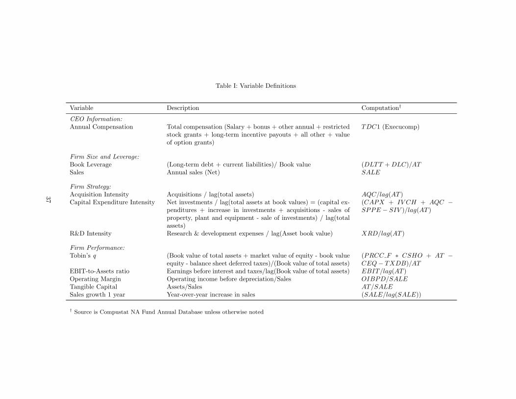
Table I: Variable Definitions

Variable Description Computation†

CEO Information:Annual Compensation Total compensation (Salary + bonus + other annual + restricted

stock grants + long-term incentive payouts + all other + valueof option grants)

TDC1 (Execucomp)

Firm Size and Leverage:Book Leverage (Long-term debt + current liabilities)/ Book value (DLTT + DLC)/ATSales Annual sales (Net) SALE

Firm Strategy:Acquisition Intensity Acquisitions / lag(total assets) AQC/lag(AT )Capital Expenditure Intensity Net investments / lag(total assets at book values) = (capital ex-

penditures + increase in investments + acquisitions - sales ofproperty, plant and equipment - sale of investments) / lag(totalassets)

(CAPX + IV CH + AQC −SPPE − SIV )/lag(AT )

R&D Intensity Research & development expenses / lag(Asset book value) XRD/lag(AT )

Firm Performance:Tobin’s q (Book value of total assets + market value of equity - book value

equity - balance sheet deferred taxes)/(Book value of total assets)(PRCC F ∗ CSHO + AT −CEQ− TXDB)/AT

EBIT-to-Assets ratio Earnings before interest and taxes/lag(Book value of total assets) EBIT/lag(AT )Operating Margin Operating income before depreciation/Sales OIBPD/SALETangible Capital Assets/Sales AT/SALESales growth 1 year Year-over-year increase in sales (SALE/lag(SALE))

† Source is Compustat NA Fund Annual Database unless otherwise noted

37

Table II: Sample Descriptive Statistics

Variable Mean SD P25 P50 P75

CEO Information:Annual Compensation ($million) 4.40 5.38 1.27 2.54 5.19Incentive Exposure (B) 20.4 38.1 4.2 8.7 19.0Age (years) 56.1 6.9 51.0 56.0 61.0Tenure (years) 6.4 5.7 3.0 5.0 9.0

Firm Size and Leverage:Book Leverage 0.22 0.18 0.07 0.21 0.32Firm Age (years) 28.2 15.5 14.0 28.0 42.0Sales ($billion) 4.6 9.0 0.5 1.4 4.2

Firm Strategy:Acquisition Intensity 0.04 0.09 0.00 0.00 0.03Capital Expenditure Intensity 0.10 0.12 0.03 0.07 0.13R and D Intensity 0.03 0.06 0.00 0.00 0.04

Firm Performance:Tobin’s q 2.04 1.24 1.26 1.64 2.37EBIT-to-Assets 0.114 0.099 0.060 0.109 0.167Operating Margin (%) 15.1 11.2 8.3 13.5 20.4Tangible Capital (assets/sales) 1.2 0.8 0.7 1.0 1.4Sales Growth 1 yr. (%) 10.5 -79.5 0.9 8.1 17.4

The table shows the mean, standard deviation (SD), and summary distributional values for a variety of CEOand firm variables in the sample. P25 shows the lower 25th percentile value for each variable. P50 representsthe median and P75 gives the upper 25th percentile value. All dollar values are in real terms as of the year2000.

38

Table III: Firm Value

The table presents results of the dynamic panel regression of future firm value and earnings on currentincentive levels and controls variables. During estimation, all variables are treated as endogenous andinstrumented as described in Section III. Z-statistics are computed using standard errors that are robustto heteroskedasticity and, when appropriate, autocorrelation of the residuals. They are adjusted for thesmall-sample properties documented by Windmeijer (2005).

(1) (2) (3) (4)Predicted Variable Tobin’s q Tobin’s q EBIT-to-Assets EBIT-to-Assets

Incentives B (x1000) 15.70* 9.98*** 0.67** 0.31**(1.83) (3.32) (2.16) (1.98)

Log Sales ($million) -1.75*** -0.09***(-4.72) (-4.27)

Acquisition Intensity -0.78 0.08(-0.88) (1.04)

Capital Expenditure Intensity 0.21 -0.11(0.27) (-1.57)

R and D Intensity 8.13** 0.62***(2.32) (2.64)

Book Leverage 1.31 0.01(1.31) (0.25)

Operating Margin 1.94** 0.09(2.02) (0.67)

Tangible Capital -0.23 -0.04***(-1.11) (-3.22)

Sales Growth 1 yr. 0.36* 0.00(1.74) (0.09)

Lag EBIT-to-Assets 0.45*** 0.35***(3.05) (3.59)

Observations 5011 4972 4140 4110Number of Number of CEO-Firm units 1341 1330 1159 1151M2 (p-value) 0.420 0.785 0.020 0.202M3 (p-value) 0.642 0.356 0.233 0.280J-test (p-value) 0.742 0.204 0.640 0.388Dummies Yr×Sector Yr×Sector Yr×Sector Yr×Sector

Windmeijer WC-robust estimatorz-statistics in parentheses

*** p < 0.01, ** p < 0.05, * p < 0.1

39

Table IV: Economic Level of Incentives

The table presents the value created by incentives as implied by the empirical results. All results are listed asraw values and as percentages of sample means and of sample standard deviations. For both Tobin’s q andEBIT-to-Assets, the elasticity of firm performance to incentive levels is taken from the empirical specificationswith control variables, columns (2) and (4), in Table III. The mean and median columns present the resultsimplied for this elasticity evaluated at the mean and median incentive levels for the sample.

Mean Median

Tobin’s q

Value 0.204 0.087

Percent of Sample Mean (%) 10.0 4.3

Percent of Sample Std. Dev. (%) 16.4 7.0

EBIT-to-Assets

Value 0.0063 0.0027

Percent of Sample Mean (%) 5.5 2.4

Percent of Sample Std. Dev. (%) 6.4 2.7

40

Table V: Firm Value and CEO Discretion

The table presents results of the dynamic panel regression of future firm value and earnings on currentincentive levels and controls variables. DiscretionRatio, as described in Section IV, is a measure of the degreeto which exercisable and tradable securities comprise the CEO’s incentive portfolio. During estimation, allvariables are treated as endogenous and instrumented as described in Section III. Z-statistics are computedusing standard errors that are robust to heteroskedasticity and, when appropriate, autocorrelation of theresiduals. They are adjusted for the small-sample properties documented by Windmeijer (2005).

(1) (2) (3) (4)Predicted Variable Tobin’s q Tobin’s q EBIT-to-Assets EBIT-to-Assets

Incentives B (x1000) 84.20*** 24.80*** 1.89 1.11**(3.33) (3.83) (0.36) (2.27)

Incentives B ·Discretion Ratio (x1000) -72.60*** -17.90*** 1.02 -0.78(-2.96) (-2.62) (0.23) (-1.60)

Discretion Ratio -0.316 -0.081 -0.133 0.008(-1.094) (-0.362) (-0.799) (0.364)

Log Sales ($million) -1.61*** -0.10***(-4.63) (-4.12)

Acquisition Intensity -0.51 -0.10(-0.63) (-1.28)

Capital Expenditure Intensity -0.10 0.07(-0.15) (1.09)

R and D Intensity 4.06 0.13(1.37) (0.64)

Book Leverage 1.23 0.00(1.22) (0.00)

Operating Margin 1.92** -0.17(2.19) (-1.50)

Tangible Capital -0.14 -0.04***(-0.74) (-2.90)

Sales Growth 1 yr. 0.37* 0.01(1.75) (0.74)

Lag EBIT-to-Assets 0.24 0.32***(0.57) (3.08)

Observations 5011 4972 4140 4110Number of Number of CEO-Firm units 1341 1330 1159 1151M2 (p-value) 0.340 0.663 0.536 0.131M3 (p-value) 0.601 0.452 0.081 0.197J-test (p-value) 0.308 0.077 0.825 0.938Dummies Yr×Sector Yr×Sector Yr×Sector Yr×Sector

Windmeijer WC-robust estimatorz-statistics in parentheses

*** p < 0.01, ** p < 0.05, * p < 0.1

41

Table VI: Economic Level of Incentives with CEO Discretion

The table presents the value created by incentives as implied by the empirical results. All results are listedas raw values and as percentages of sample means and of sample standard deviations. For both Tobin’s qand EBIT-to-Assets, the elasticities of firm performance to incentive levels and to incentives interracted withdiscretion are taken from the empirical specifications with control variables, columns (2) and (4), in TableV. The mean and median columns present the results implied at the mean and median incentive levels forthe sample. These incentive levels are then interacted at the empirically observed 25th percentile, median,and 75th precentile of CEO discretion.

Mean Incentives Median IncentivesDiscretion Ratio Quantile 25th Median 75th 25th Median 75th

Tobin’s q

Value 0.303 0.237 0.180 0.129 0.101 0.077

Percent of Sample Mean (%) 14.8 11.6 8.8 6.3 4.9 3.8

Percent of Sample Std. Dev. (%) 24.4 19.1 14.5 10.4 8.1 6.2

EBIT-to-Assets

Value 0.0138 0.0109 0.0084 0.0059 0.0047 0.0036

Percent of Sample Mean (%) 12.1 9.6 7.4 5.2 4.1 3.2

Percent of Sample Std. Dev. (%) 13.9 11.0 8.5 5.9 4.7 3.6

42

Table VII: Firm Value: Robustness, Alternate Economic Group Definitions

The table presents results of the dynamic panel regression of future firm value on current incentive levelsand controls variables. While the main specification used in the paper adjusts for 8 time-varying sectormeans, columns (1) and (2) of this table account for 19 time-varying group means. Columns (3) and (4)account for 64 time-varying industry means. During estimation, all variables are treated as endogenous andinstrumented as described in Section III. Z-statistics are computed using standard errors that are robustto heteroskedasticity and, when appropriate, autocorrelation of the residuals. They are adjusted for thesmall-sample properties documented by Windmeijer (2005).

(1) (2) (3) (4)Predicted Variable Tobin’s q Tobin’s q Tobin’s q Tobin’s q

Incentives B (x1000) 11.80* 6.65** 20.00 5.75**(1.68) (2.47) (0.24) (2.12)

Log Sales ($million) -1.81*** -1.80***(-5.05) (-5.48)

Acquisition Intensity -0.27 -1.04(-0.33) (-1.20)

Capital Expenditure Intensity -0.06 0.77(-0.09) (1.05)

R and D Intensity 8.05** 8.55***(2.44) (2.78)

Book Leverage 1.06 1.08(1.06) (1.42)

Operating Margin 2.15** 2.18**(2.33) (2.34)

Tangible Capital -0.21 -0.12(-1.07) (-0.78)

Sales Growth 1 yr. 0.36 0.33(1.54) (1.37)

Observations 5011 4972 5011 4972Number of Number of CEO-Firm units 1341 1330 1341 1330M2 (p-value) 0.382 0.887 0.942 0.636M3 (p-value) 0.580 0.274 0.705 0.555J-test (p-value) 0.667 0.325 1.000 1.000Dummies Yr×Group Yr×Group Yr×Industry Yr×Industry

Windmeijer WC-robust estimatorz-statistics in parentheses

*** p < 0.01, ** p < 0.05, * p < 0.1

43

Table VIII: Firm Value: Robustness, Fama-French Excess Return Instruments

The table presents results of the dynamic panel regression of future firm value and earnings on current incen-tive levels and control variables. During estimation, all variables are treated as endogenous and instrumentedas described in Section III. For this robustness test, stock return instruments are computed using the annualexcess returns from Fama-French three-factor regressions averaged over firms in each company’s economicsubgroup. Z-statistics are computed using standard errors that are robust to heteroskedasticity and, whenappropriate, autocorrelation of the residuals. They are adjusted for the small-sample properties documentedby Windmeijer (2005).

(1) (2) (3) (4)Predicted Variable Tobin’s q Tobin’s q EBIT-to-Assets EBIT-to-Assets

Incentives B (x1000) 11.40* 8.86*** 0.65** 0.25*(1.86) (3.20) (2.02) (1.77)

Log Sales ($million) -1.66*** -0.08***(-4.93) (-4.02)

Acquisition Intensity 0.01 0.06(0.01) (0.77)

Capital Expenditure Intensity -0.29 -0.09(-0.42) (-1.53)

R and D Intensity 7.42** 0.58**(2.29) (2.49)

Book Leverage 1.09 0.02(1.41) (0.42)

Operating Margin 1.37 0.06(1.39) (0.53)

Tangible Capital -0.28 -0.04***(-1.64) (-3.08)

Sales Growth 1 yr. 0.36* -0.00(1.89) (-0.04)

Lag EBIT-to-Assets 0.38** 0.37***(2.54) (3.66)

Observations 5215 5173 4309 4277Number of Number of CEO-Firm units 1395 1384 1218 1210M2 (p-value) 0.388 0.811 0.008 0.142M3 (p-value) 0.551 0.343 0.183 0.284J-test (p-value) 0.656 0.053 0.173 0.255Dummies Yr×Sector Yr×Sector Yr×Sector Yr×Sector

Windmeijer WC-robust estimatorz-statistics in parentheses

*** p < 0.01, ** p < 0.05, * p < 0.1

44