How Much Can Taxation Alleviate

Temptation and Self-Control Problems?

Per Krusell,Burhanettin Kuruscu,

andAnthony A. Smith, Jr.∗

May 2009

AbstractWe develop a quantitative dynamic general-equilibrium model where agents have preferences

featuring temptation and self-control problems, and we apply it in order to understand to whatextent standard investment/savings subsidies can improve welfare.

The dynamic model of preferences builds on the Gul-Pesendorfer setting and uses a “quasi-geometric” formulation for temptation, the strength of which is modeled with a separate param-eter. When this parameter is infinity, consumers always succumb to the temptation, and ourformulation reduces to the model of multiple selves studied elsewhere. We embed the consumerin the typical neoclassical growth setting used for macroeconomic analysis and demonstratehow steady states can be analyzed and how equilibria can be solved. We also propose a way ofcalibrating the model.

Our preference-based setting gives unequivocal guidance for policy analysis. In our quan-titative application, we show that when preferences are such that self-control is limited andconsumers instead mainly succumb to the temptation of overconsumption, policy can play animportant role.

∗This paper performs the quantitative analysis formerly studied in a paper entitled “Temptation and Tax-ation”; that paper, thoroughly revised, now focuses solely on theoretical analysis of optimal taxation withtemptation and self-control problems. We thank Daron Acemoglu, Larry Epstein, Xavier Gabaix, WolfgangPesendorfer, Ivan Werning, Justin Wolfers, and three anonymous referees for important suggestions and com-ments. Krusell, Kuruscu, and Smith are at the Institute for International Economic Studies (Stockholm), theUniversity of Texas at Austin, and Yale University, respectively. We thank seminar participants at ArizonaState University, Brown University, Carnegie Mellon University, Duke University, Harvard University, Insti-tute for International Economic Studies, Johns Hopkins University, Federal Reserve Bank of Kansas City,Massachusetts Institute of Technology, Universite de Montreal, New York University, Princeton University,Stanford University, University of Virginia, Yale University, and the 2001 North American Summer Meetingsof the Econometric Society and Society for Economic Dynamics conferences for helpful comments. Kruselland Smith thank the National Science Foundation for financial support.

1 Introduction

Recently, the experimental evidence from the psychology literature has attracted increasing atten-

tion from economists. In particular, the so-called “preference reversals” observed in laboratory

settings have been interpreted as evidence that a new model of intertemporal decision making is

needed. Since a core part of the way we analyze macroeconomic growth in the short and in the

long run rests on the standard geometric-discounting model of consumption-savings decisions, what

should macroeconomists take away from the experimental evidence? Barro (1999) argues that one of

the new models that can allow for reversals—the multiple-selves model developed by Strotz (1956),

Phelps and Pollak (1968), and Laibson (1994)—in its macroeconomic form in several important

cases is observationally equivalent, or near-equivalent, to the standard model. However, even if

Barro is right, we would still be left with an important question, namely that of how to conduct

economic policy: should the government intervene in markets to alter individual, and aggregate,

savings outcomes? In particular, should governments subsidize savings to correct the “present-bias”

suggested in the laboratory experiments? In this paper, we develop a dynamic, general-equilibrium

setting designed to address questions of this sort.

Although the multiple-selves model can account successfully for preference reversals, it is not

obvious how to use it for normative analysis: whose utility should the government maximize?

Though one can argue that, under some circumstances, the utility levels of all selves can be in-

creased by subsidizing savings, this still leaves open how to answer the quantitative part of our

question.1 Thus, we need to tackle this issue in order to proceed. Recently, Gul and Pesendorfer

(2001) have developed another model—one based entirely on revealed preference and for which it

is therefore clear how to evaluate welfare—that also delivers present-bias. Gul and Pesendorfer’s

model, moreover, formalizes the concepts of temptation and self-control, which in part are distinct

from those emphasized in the multiple-selves setup. We adopt Gul and Pesendorfer’s approach

here, though an important part of our analysis has to do with how their model compares with the

multiple-selves model, particularly in terms of its welfare implications.

To implement the GP (Gul-Pesendorfer) approach in our macroeconomic context, it is neces-

sary to develop it in a number of ways. The GP model builds on the idea that agents suffer from

temptation/self-control problems. However, the basic GP formulation is quite general so our first

task is to specialize it. In particular, we need to specialize agents’ temptation problems: what form

does temptation take? We assume that consumers are tempted by (or find tempting) a high level

of current relative to future consumption, but are not tempted by alternative rankings of future

consumption streams.2 We show that, as a special case, this setup actually reproduces multiple-

selves-like behavior. The GP framework, therefore, can be viewed as providing a microfoundation

for the multiple-selves model: it provides a formal theory of some of the “deeper cognitive sub-1See Laibson (1996).2This contrasts Noor (2005), who considers a richer setup.

1

components of the struggle for self-command” (Angeletos et al [2001], p. 65). More importantly,

this setup naturally suggests how welfare should be measured in the context of the multiple-selves

model.3

An important feature of our setup is its parsimony: in our specialization of the GP framework,

the new psychological factors that it emphasizes—temptation and self-control—can be summarized

with two new parameters. One of these describes the nature of temptation (β, as in the β-δ,

or quasi-geometric-discounting, formulation), and the other describes the strength of temptation

(γ). The multiple-selves special case appears as γ goes to infinity, so that the agent succumbs to

temptation, without exercising any self-control.4 We investigate the separate roles of β and γ from

a positive as well as normative perspective.

The GP approach builds on the idea that when an agent chooses from a set, the size and shape of

the set influence utility, since this set rooms any potentially tempting, though perhaps not chosen,

alternative. If, in particular, especially tempting allocations are available in the set, utility in an

ex ante sense is lower: it would be better to choose out of a smaller set. In a dynamic model, these

aspects of the set actually influence behavior earlier on, to the extent that earlier behavior can

influence the shape of subsequent choice sets. Thus, the specification of the choice set is crucial.

Here, we wish to adhere as closely as possible to standard dynamic competitive neoclassical analysis

by assuming that agents are price takers and face typical sequential budget constraints.5 Thus, tax

policy—assuming, as we do, that taxes are proportional—amounts to the changing of the slopes

and intercepts of these sets.

Analyzing a long-horizon version of the GP model with neoclassical production and perfect

competition is a nontrivial task, in part because it always involves analyzing the implications of

temptations—how the individual would behave if he succumbed to temptation. Though conceptu-

ally different, temptation behavior is like “off-equilibrium-path behavior” in that it is not observed

but nevertheless important in determining what is observed. The dynamic implications of succumb-

ing to temptation, and the benefits from decreasing future temptation by altering current savings,

are thus in focus here. We show that the consumption-savings problem can be summarized by a

pair of Euler equations—one for actual and one for temptation behavior—each of which explicitly

incorporates how the agent’s current savings are chosen taking into account how they influence

future costs of self-control. Fortunately, we are also able to show that under standard restrictions

on the curvature of period utility—period utility is a power function of consumption—there is a

closed-form solution to the agent’s decision problem. This result builds on “aggregation” argu-3As we discuss in greater detail below, it turns out that welfare in the GP framework corresponds closely to the

“long-run perspective” advocated by O’Donoghue and Rabin (1999) in the context of the multiple-selves model; seealso Schelling (1984) and Akerlof (1991).

4We prove this formally given a set of functional-form assumptions. Gul and Pesendorfer (2005) study this limitingcase in detail from an axiomatic perspective.

5Esteban and Miyagawa (2003,2004) consider nonlinear pricing and more complex choice sets in an interestingapplication to “supermarket shopping”. Similar ideas could be applied to shopping for different savings plans, butwe nevertheless find it useful to first organize the ideas here in the context of a more standard benchmark.

2

ments: savings are linear in private wealth. That is, we adopt a formulation that we show inherits

useful features of optimal savings in the corresponding model without preference reversals.

When analyzing our macroeconomic general-equilibrium problem, we need to deliver an analysis

both of steady states and of the dynamics that lead to steady state. We first characterize steady

states. This is possible to do analytically for all values of our curvature parameter despite the

fact that the steady state depends on temptation behavior, which is to move away from steady

state toward lower levels of capital. In our analysis of transition we show both that it is possible

to find closed-form solutions in special cases (assuming logarithmic curvature in preferences and

a Cobb-Douglas production function with full depreciation) and we develop a way of solving the

model numerically in other cases. For the special functional-form case, we demonstrate a parallel

of Barro’s result, namely observational equivalence with the standard model (and, given Barro’s

finding, with the quasi-geometric-discounting model). Differences appear under any curvature

other than the logarithmic one, but moderate departures from it generate only small differences

in observable implications between the present and the standard model. We take comfort in this:

we do not primarily propose the present model in order to better match data given standard

competitive budget sets, but rather as a tool for normative analysis in a quantitative setting.

Our quantitative policy analysis requires parameter selection. Specifically, we need to determine

not only the equivalent of our standard discounting parameter (labeled δ here) but also the β and the

γ that express the nature and strength of temptation. In the absence of more elaborate experimental

evidence than the one suggested above—which is mainly qualitative—we rely on a combination of

introspective questions and robustness checks. More precisely, we pose two quantitative questions

to a presumptive consumer in the steady state of our model, the answers to which pin down our

temptation and self-control parameters: we offer the consumer more “tools” for consumption-

savings decisions and then ask how much he would be willing to pay for these tools.

The first question is how much (normalized in some appropriate way) the consumer would be

willing to pay in order to obtain full commitment to future consumption levels and hence to be able

to choose these future consumption levels now, subject only to the present-value budget constraint.

A standard consumer would answer zero, but a consumer with temptation/self-control problems

would, as shown by Gul and Pesendorfer, show a “preference for commitment”: his answer would

be positive, reflecting a wish both to increase savings at future dates and to eliminate costs of

self-control at all dates. A consumer in the multiple-selves model (a “Laibson” consumer) would

also give a positive answer to this question: he would find it beneficial to commit his future selves

to higher savings.

The second question we pose, however, does allow us to distinguish Laibson consumers from

GP consumers: it asks how much consumers would be willing to pay to obtain full commitment

to the consumption path the consumer would have chosen anyway. That is, by offering to replace

the sequence of budget sets with one point only—the one currently planned, in the absence of any

commitment device—it allows no temptation and thus it simply asks what the costs of self-control

3

are in the consumer’s present situation. Since Laibson consumers can be viewed as succumbing

completely to temptation, these consumers do not have a cost of self-control: they are not influenced

by the parts of the constraint set that are not chosen. Hence, their answer would be zero. GP

consumers, on the other hand, would be willing to pay anything between zero and the answer to the

first question (the first question leads to an answer with a larger welfare gain since the consumer

would also be able to affect this actual consumption). In sum, though as far as we are aware these

two questions have not been posed in any actual laboratory environments, they would allow us to

learn significantly more about preferences and, in particular, they allow the reader of this paper to

use introspection in order to assess the plausibility of our different calibrations. For the rest of our

model parameters, we use a calibration in line with the rest of the macroeconomic literature.

Our quantitative results show that the government should, presuming that consumers have GP

preferences, subsidize savings and thus raise the long-run level of capital in the economy. The

amount of these subsidies are, of course, a function of the calibrated β and γ. Consider first a

Laibson consumer, i.e., a consumer who has a γ equal to infinity, thus succumbing to temptation

fully. Let the extent of the present-bias be that suggested in Laibson’s own work (e.g., Laibson,

Repeto, and Tobacman (2004), who suggests a β of around 0.7); such a preference parameter

would result if consumers would value commitment as being equivalent to having a permanent

consumption increase of 6%. Then the optimal subsidy—defined on all asset savings—is a little

over 2%.6 The subsidy level falls quite drastically, however, if there are also self-control costs: if the

second question above is answered with a number close to that of the first, i.e., if the consumer suffers

almost exclusively from the pains of self-control, then government subsidies can do little to improve

on market outcomes; optimal subsidy rates fall to close to zero. More generally, suppose that

the consumer answers the first question with y% (i.e., he would consider commitment equivalent

to a permanent consumption increase of y%) and the second with x% (i.e., he would consider

commitment to the present allocation equivalent to a permanent consumption increase of x%). We

find that the optimal subsidy depends mainly on the difference y − x. In other words, tax policy

is simply not a convenient tool for eliminating costs of self-control, but it is effective for inducing

consumers to choose differently: the tax rate offers incentives similar in realized outcomes to what

would occur were the consumer given access to commitment. Finally, we find that the curvature of

the period utility function does not seem to be of first-order importance for the results.

Our paper is organized as follows. In Section 2, we develop our version of the Gul-Pesendorfer

model and embed it in a neoclassical setting: Section 2.2 studies a simple two-period model illus-

trating how to think about temptation and self-control in the consumption-savings setting with

production, Section 2.3 looks at longer time horizons and introduces the notion of quasi-geometric

temptation, and Section 2.3.2 contains the analysis of a dynamic competitive equilibrium, includ-

ing the characterization of steady states and transition dynamics. Section 3 contains the policy6The tax base of course matters. In the case of a subsidy to all capital and labor income, one would require a rate

of about 7%.

4

analysis: Sections 3.1 and 3.2 develop the equilibrium with taxes and show how to solve it; Section

3.3 explains how we calibrate the parameters governing temptation and self-control; and Section

3.4 presents the quantitative findings about optimal taxation. Section 4 concludes. An appendix

contains all proofs.

2 A dynamic model of temptation and self-control

In this section we develop a dynamic model of temptation and self-control. This model is a special-

ization of the model of temptation and self-control developed by Gul and Pesendorfer (2001, 2004).

In particular, we assume that consumers have quasi-geometric temptations. In Krusell, Kuruscu,

and Smith (2009), we study the qualitative features of optimal taxation in a finite-horizon model

of temptation and self-control. Our purpose here is to study competitive equilibria and optimal

taxation in a quantitative infinite-horizon model with quasi-geometric temptation.

To keep the presentation self-contained, we first provide a brief overview of Gul and Pesendorfer’s

model; those readers who are already familiar with this model may safely skip the overview. We

then describe the finite-horizon model studied in Krusell, Kuruscu, and Smith (2009), before turning

to a description of our infinite-horizon model.

2.1 Temptation, self-control, and the Gul-Pesendorfer model

Gul and Pesendorfer (2001) axiomatize the notions of temptation and self-control by imagining that

consumers have preferences over sets of lotteries. In this section, we provide a brief, nontechnical

overview of Gul and Pesendorfer’s ideas. To understand the way in which Gul and Pesendorfer

model preferences over choice sets, it is helpful to think of each period being divided into two

subperiods: in the first subperiod, the consumer chooses a choice set; in the second subperiod, the

consumer makes a consumption choice from this set. In a consumption-savings problem, today’s

consumption choice determines the set from which next period’s consumption choice is made.

To see how Gul and Pesendorfer model preferences over choice sets, begin in the second subpe-

riod by allowing utility to depend not only on the choice x but also on the set A from which x is

chosen. Given preferences over pairs of the form (A, x), Gul and Pesendorfer say that a choice y

“tempts” a choice x if ({x}, x) is preferred to ({x, y}, x). Gul and Pesendorfer place structure on

the nature of temptation by assuming that: one, removing temptations cannot make the consumer

worse off; two, if y tempts x, then x does not tempt y; and, three, adding y to A does not make the

consumer worse off unless y tempts every element in A. These assumptions imply that “tempts”

is a preference relation and, moreover, that the utility of a fixed choice is affected by the choice set

only through its most tempting element.

Preferences in the second subperiod induce preferences in the first subperiod over choice sets

themselves: for any two choice sets A and B, A � B if and only if there is an x ∈ A such that (A, x)

is (weakly) preferred to (B, y) for all y ∈ B. Given Gul and Pesendorfer’s assumptions, preferences

5

over choice sets satisfy what Gul and Pesendorfer call “set betweenness”: A � B implies that A �A ∪ B � B. Gul and Pesendorfer show that their formalization of temptation and self-control is,

in fact, equivalent to “set betweenness”.

The central implication of set betweenness is that choice sets cannot be compared simply by

looking at their best elements. It is possible, instead, that a consumer strictly prefers a given set

to another, larger set of which the first set is a strict subset .

More specifically, set betweenness allows for three possibilities. First, there is the standard case:

A ∼ A ∪ B � B. In this case, with the preferred consumption bundle being in A, the addition of

the set B to the set A is irrelevant.

Second, the consumer could have a preference for commitment and yet “succumb” to “temp-

tation” when it is present: A � A ∪ B ∼ B. In this case, because A is preferred to A ∪ B, the

consumer is made worse off by the addition of the set B: he would prefer to commit to the smaller

choice set A. Nonetheless, the consumer succumbs to temptation when faced with the choice set

A ∪ B: he is indifferent between B and A ∪ B because he knows that if his choice set is A ∪ B he

will succumb to the temptation contained in B.

Third and finally, the consumer could have a preference for commitment and yet exert self-

control when faced with tempting alternatives: A � A ∪ B � B. In this case, the consumer has

enough self-control not to succumb to the temptation contained in B and yet he nonetheless prefers

the smaller set A to the larger one A ∪ B because exerting self-control is costly (i.e., reduces his

utility).

Under the axioms that Gul and Pesendorfer adopt—appropriately modified versions of standard

axioms (completeness, transitivity, continuity, and independence) together with set betweenness—

they show that preferences in the second subperiod can be represented as follows:

W ∗(A, x) = U(x) + V (x)−maxx∈A

V (x),

where W ∗(A, x) is the utility that the consumer associates with choice x made from set A. These

preferences induce the following representation of preferences over choice sets themselves:

W (A) = maxx∈A

{U(x) + V (x)} −maxx∈A

V (x),

where W (A) is the utility that the consumer associates with set A. In these representations, U

determines the commitment ranking (i.e., the utility of singleton sets), while V determines the

temptation ranking (i.e., V gives higher values to more tempting elements).

The consumer’s optimal action is determined by arg maxa∈A {U(a) + V (a)}, but the utility of

this action depends on the amount of self-control that the consumer exerts when he makes this

choice. In particular, V (a)−maxa∈A V (a) ≤ 0 can be viewed as the disutility of self-control given

that the consumer chooses action a. If arg maxa∈A {U(a) + V (a)} = arg maxa∈A V (a), then either,

one, we are in a standard case (U = V ) where temptation and self-control play no role in the

6

consumer’s decision-making or, two, the agent succumbs, i.e., lets V govern his choices completely.

If, on the other hand, the two argmaxes are not the same, then the consumer exercises self-control.

2.2 The two-period consumption-savings model with temptation

As in Krusell, Kuruscu, and Smith (2009), we now specialize the general framework described in

Section 2.1 to a simple two-period general equilibrium economy with production. This example

allows us to illustrate the role of temptation and self-control in determining equilibrium outcomes

before turning to a fully dynamic economy in the next section.

2.2.1 Preferences: the form of temptation

A typical consumer in the economy values consumption today (c1) and tomorrow (c2). Specifically,

the consumer has Gul-Pesendorfer preferences represented by two functions u(c1, c2) and v(c1, c2);

these functions are the counterparts of U and V , respectively, in Section 2.1.

We specify the functions u and v as follows:

u(c1, c2) = u(c1) + δu(c2)

and

v(c1, c2) = γ(u(c1) + βδu(c2)),

where u has the usual properties and 0 < β ≤ 1. When β = 1, we have the standard model in

which temptation and self-control do not play a role. When β < 1, however, the temptation function

gives a stronger preference for present consumption. The strength of this preference increases as γ

increases. The decision problem of a typical consumer, then, is:

maxc1,c2

{u(c1, c2) + v(c1, c2)} −maxc1,c2

v(c1, c2) (1)

subject to a budget constraint that we will specify below.

2.2.2 Competitive equilibrium

Each consumer is endowed with k1 units of capital at the beginning of the first period and with one

unit of labor in each period. Each consumer rents these factors of production to a profit-maximizing

firm that operates a neoclassical production function. In equilibrium, given aggregate capital k, the

rental rate r(k) and the wage rate w(k) are determined by the firm’s marginal product conditions.

Given these prices, the consumer’s budget constraint is described by the set:

B(k1, k1, k2) ≡ {(c1, c2) : ∃k2 : c1 = r(k1)k1 + w(k1)− k2 and

c2 = r(k2)k2 + w(k2)}

where k2 is the consumer’s asset holding at the beginning of period 2 (i.e., his savings in period 1)

and ki is aggregate capital in period i. Since all consumers have the same capital holdings in period

7

1, k1 = k1; in equilibrium, k2 = k2, but when choosing k2 the consumer takes k2 as given. Inserting

the definitions of the functions u and v into (1) and combining terms, a typical consumer’s decision

problem is:

max(c1,c2)∈B(k1,k1,k2)

{(1 + γ)u(c1) + δ(1 + βγ)u(c2)} − max(c1,c2)∈B(k1,k1,k2)

γ{u(c1) + βδu(c2)}. (2)

In this two-period problem, the “temptation” part of the problem (i.e., the second maximization

problem in the objective function) plays no role in determining the consumer’s actions in period 1.

As we describe in Section 2.3, this is not true when the horizon is longer than two periods. The

temptation part of the problem does, however, affect the consumer’s welfare, as we discuss below.

The consumer’s intertemporal first-order condition is:

(1 + γ)(1 + βγ)δ

u′(c1)u′(c2)

= r(k2).

It is straightforward to see that the intertemporal consumption allocation (which, in effect, max-

imizes u + v) represents a compromise between maximizing u = u(c1) + δu(c2) and maximizing

v = u(c1) + βδu(c2). In the former case, the first-order condition is:

1δ

u′(c1)u′(c2)

= r(k2),

whereas in the latter case, the first-order condition is:

1βδ

u′(c1)u′(c2)

= r(k2).

Since1βδ

≥ (1 + γ)(1 + βγ)δ

≥ 1δ,

the consumer’s consumption allocation is tilted towards the present relative to maximizing u(c1) +

δu(c2) and is tilted towards the future relative to maximizing the temptation function u(c1) +

βδu(c2).

To determine the competitive equilibrium allocation, set k2 = k2 in the consumer’s first-order

condition and recognize that r(k) = 1−d+f ′(k), where f is the firm’s production function (which

has the standard properties) and d is the depreciation rate of capital. To wit,

(1 + γ)(1 + βγ)δ

u′(c1)u′(c2)

= 1− d + f ′(k2),

where ci is aggregate (per capita) consumption in period i.

2.3 Longer time horizons

We now extend the Gul-Pesendorfer preference formulation considered above to an arbitrary finite-

horizon setting. In addition to generalizing the setting, this development provides a framework

8

for the later analysis of policy, which is quantitative in spirit. Thus, the model presented below

can be viewed as the neoclassical growth model extended to allow preferences with temptation and

self-control.

We begin by showing how to use recursive methods to formulate the sequence of decision

problems when there is temptation and self-control. The temptation we consider is one which

is closely related to and, in a precise sense, nests the multiple-selves model: we call it “quasi-

geometric temptation”. This formulation also makes clear how to conduct the normative analysis

later, including in the special case where a model formulation based on multiple selves leaves

open whose utility to focus on. Next, we characterize the agent’s behavior in terms of first-order

conditions which are readily interpretable. We then go on to specify and show how to solve for

general-equilibrium outcomes using a representative-agent construct.

2.3.1 The general case: a recursive formulation

We now look at an economy with an arbitrary horizon. For notational simplicity, we first focus on

an “autarky” (or Robinson Crusoe) model with full depreciation. As in the two-period model in

Section 2.2, we use capital rather than present-value wealth as a state variable (we do this merely

for notational convenience). Thus we have

Wt(k) = maxk′≤f(k)

{u(f(k)− k′) + δWt+1(k′) + Vt+1(k, k′)} − maxk′≤f(k)

{Vt+1(k, k′)}, (3)

where the temptation function Vt is quasi-geometric:

Vt(k, k′) ≡ γ{u(f(k)− k′) + βδWt+1(k′)}.

These equations hold for t = 0, 1, 2, . . . , T − 1, where T is the final period in which consumption

takes place; VT and WT are both zero for all values of their arguments. We let gt(k) denote the

decision rule for the agent, i.e., the function that is the argmax of the first maximization problem

in the period-t formulation of equation (3). Similarly, we let gt(k) be the argmax in the temptation

problem, i.e., the second maximization problem in (3).

Notice that when γ = 0 or β = 1, we have as a special case the standard model without

temptation or self-control. When β < 1, we can approach the multiple-selves model by making γ

large: as γ goes to infinity, the consumer puts so much weight on the temptation that he succumbs.

This limiting case is appealing because it provides one way to evaluate policy in the multiple-selves

model. That is, this case provides a potential resolution to the problem of which of the consumer’s

“selves” should be used when assessing welfare.

First-order conditions. Before studying these parametric examples, however, it might be in-

structive to derive the Euler equations associated with the problem defined by (3). Since we must

determine two “decision rules” (one for each of the maximization problems on the right-hand side

9

of (3)), there are two Euler equations. The first one is the condition that pins down actual con-

sumption:

u′(ct) = δ1 + βγ

1 + γf ′(kt+1){u′(ct+1) + γ[u′(ct+1)− u′(ct+1)]}, (4)

where ct ≡ f(kt) − gt(kt) and ct+1 ≡ f(kt+1) − gt+1(kt+1) are the actual consumption levels and

ct+1 ≡ f(kt+1)− gt+1(kt+1) is temptation consumption next period.

The second Euler equation, which pins down temptation consumption, reads

u′(ct) = βδf ′(gt(kt)){u′(ct+1) + γ[u′(ct+1)− u′(˜ct+1)]}.

Here ct ≡ f(kt)−gt(kt) and ct+1 ≡ f(gt(kt))−gt+1(gt(kt)) are period-t and period-t+1 consumption

levels in the hypothetical case that the consumer were to succumb at t given a capital stock kt, and˜ct+1 ≡ f(gt(kt)) − gt+1(gt(kt)) is next period’s temptation consumption given that you succumb

today.7

Both these expressions look like standard Euler equations except in two places: (i) the discount

factors; and (ii) the added term γ(u′t+1− u′t+1). The discount factors, which are ranked (given that

1 > 1+βγ1+γ > β), show that the temptation discount factor is lower than that of the actual one,

provided β < 1. The term γ(u′t+1 − u′t+1) is the derivative of the disutility/cost of self-control,

γ(ut+1 − ut+1), with respect to wealth. This term is positive, since temptation consumption is

higher than actual consumption and the utility function is strictly concave. The interpretation

of these equations is that the marginal benefit from wealth tomorrow exceeds u′t+1, because the

self-control cost gets smaller as wealth increases in this model.

The idea that the marginal future benefit of wealth exceeds the marginal felicity is parallel to

what occurs in the multiple-selves model when behavior is “sophisticated”. The multiple-selves

model yields an Euler equation which reads

u′(ct) = βδu′(ct+1){f ′(kt+1) + (1/β − 1)g′m,t+1(kt+1)},

where gm,t(k) is the period-t savings given a capital stock of k and, thus, gm,t+1(kt+1) > 0 is the

marginal savings propensity in the next period.8 Here, there is an added benefit to savings, too: so

long as β < 1, the benefit arises due to the disagreement between the current and the next selves.

Any unit of wealth next period will decrease consumption that period (by an amount g′m,t+1, so

g′m,t+1u′t+1 measured in t + 1 utils). In return, it will increase consumption thereafter. The future

consumption increase is normally worth the same amount in present value (g′m,t+1u′t+1) from the

first-order condition of next period’s savings choice: the envelope theorem. In the multiple-selves

model, however, it is valued higher by the current self by a factor 1/β, since the next self, who

makes the savings decision in question, has an additional weight β on every utility flow from t + 2

and on. So, like in the Gul-Pesendorfer model, the consumers in the multiple-selves model perceive

a cost involving future savings—they are too low—and higher current savings decrease this cost.7Notice that ct+1 has conceptually different meanings in the two Euler equations.8The subscript ‘m’ on g in this equation denotes “multiple-selves.” For an analysis of this Euler equation, including

numerical tools for solving it, see Krusell, Kuruscu, and Smith (2002a).

10

Infinite-horizon models. Our focus on long-horizon frameworks is motivated by quantitative

concerns. As in much of classical growth theory, the idea is to view the theory as depicting a

real-world economy which is an “ongoing” one where a final date is sufficiently far in the future

that details of when it occurs do not influence the behavior of the current economy. Thus, our

quantitative study is based on economies where the time horizon is, for practical purposes, infinite.

That is, we look at the limit of finite-horizon competitive equilibria. If such a limit exists, it will

also satisfy a stationary version of the recursive formulation in (3), i.e., where Wt = Wt+1 = W . In

practice, this means that we will often directly analyze this stationary problem as a way of finding

the limit of finite-horizon equilibria. In the sections which will follow we will also, mainly for ease of

notation, focus directly on finding W as a fixed point of this functional equation and the associated

stationary policy rules g and g.

A few remarks of caution are in order at this point, because the present model is quite different

than the standard macroeconomic framework based on preferences without temptation and self-

control. In particular, it is not a foregone conclusion that behavior converges as the time horizon

of the model goes to infinity. I.e., it is not clear that gt(k) converges to a time-invariant function

as t goes to infinity. In particular, the operator that maps Wt+1 into Wt, defined by equation (3),

does not satisfy Blackwell’s sufficient conditions for this mapping to be a contraction mapping,

which is the property typically used to establish convergence in the standard case where where

β = 1 or γ = 0. Although the mapping does satisfy discounting, it is not monotone in general. A

failure of monotonicity can occur because a greater utility from future wealth may imply lower total

utility since the disutility from self-control may increase with the higher temptation resulting from

a higher utility from future wealth. We have not been able to find a general result of convergence

except in special cases. We have, however, for the cases we study below, ways of verifying that

the fixed point to the stationary problem indeed is a limit of finite-horizon economies, because we

employ functional forms that admit taking limits explicitly. These checks are important, because

we have also been able to construct cases for which a unique fixed point W exists but where Wt

does not converge.9 The functional equation given by the stationary version of (3) can also admit

multiple solutions for W , in a manner reminiscent of the findings of Krusell and Smith (2003) for

the multiple-selves model.10

When β = 0, which is an interesting special case, monotonicity is satisfied and the contraction9To construct an example in which a unique fixed point exists and yet iteration on (3) does not converge, consider

an environment in which capital is constrained to belong to the set {k1, k2}. Let uij be the consumer’s utility whenhe has capital ki today and capital kj tomorrow. Set u11 = 1, u12 = 0.2533, u21 = 1.7889, and u22 = 1.5386. Thesevalues satisfy the requirements of consumption-savings problem (u21 > u11 > u12 and u21 > u22 > u12) and ofconcavity (u21 − u22 < u11 − u12). In addition, set β = 0.6592 and δ = 0.769. Represent a fixed point by a pairof ordered pairs ((i, j), (n, m)), where the first ordered pair is the realized (or actual) decision rule and the secondordered pair is the temptation decision rule. For example, (i, j) means that the actual decision rule is to go to state ifrom state 1 to state j from state 2. Then for this example one can verify that the unique fixed point is ((2, 2), (1, 2))and yet backwards iteration oscillates between ((1, 2), (1, 2)) and ((2, 2), (2, 2)).

10It is straightforward, for example, to find examples of multiplicity (provided β < 1) when the state space isdiscrete and γ is sufficiently large. Unlike in Krusell and Smith (2003), “mixing” solutions typically do not appearto be regular equilibria.

11

mapping theorem holds, in which case the functional equation does have a unique solution. When

β = 0, the consumer is tempted to consume all of his wealth immediately, so that this special

case is similar in some respects to the case developed in Gul and Pesendorfer (2004) (in which the

temptation depends only on current consumption). Here, however, the temptation function is a

multiple γ of u, where u is the “usual” concave period utility function rather than an arbitrary

convex function of current consumption. The free parameter γ can then be varied to calibrate the

strength of the temptation (just as β can be varied in the multiple-selves model).

2.3.2 Dynamic competitive equilibrium

We now study competitive equilibrium with quasi-geometric temptation under a long horizon, which

we take to be infinite. We use time-invariant functions to characterize the equilibrium. A typical

consumer takes factor prices (r(k) = 1 − d + f ′(k) and w(k) = f(k) − kf ′(k)) and an aggregate

law of motion k′ = G(k) as given. His decision problem can be characterized recursively as follows:

W (k, k) = maxk′{u(r(k)k + w(k)− k′) + δW (k′, k′) + V (k, k′, k, k′)} − (5)

maxk′{V (k, k′, k, k′)},

where

V (k, k′, k, k′) = γ(u(r(k)k + w(k)− k′) + βδW (k′, k′)

).

Substituting the temptation function into (5) and combining terms, the consumer’s problem be-

comes

W (k, k) = maxk′{(1 + γ)u(r(k)k + w(k)− k′) + δ(1 + βγ)W (k′, k′)} −

γ maxk′{u(r(k)k + w(k)− k′) + βδW (k′, k′)}.

Ignoring possible multiplicity for the moment, this problem determines a “realized” decision rule

g(k, k) which solves the first maximization problem and a “temptation” decision rule g(k, k) which

solves the second maximization problem. In equilibrium, we require g(k, k) = G(k).

We will now consider two special parametric examples. First, we consider the case of isoelastic

utility: u(c) = (1 − σ)−1c1−σ, where σ > 0. This case is important, as it is a very common

preference formulation in quantitative macroeconomic analysis. Later, we consider the “log-Cobb”

model: u is logarithmic, capital depreciates fully in one period, and the production function is

Cobb-Douglas. For the case of isoelastic utility, we can obtain a complete characterization of the

steady state in the competitive equilibrium and a partial characterization of the dynamic behavior

of the competitive equilibrium. For the log-Cobb model, we can obtain a complete characterization

of both steady states and dynamics.

12

Isoelastic utility and any convex technology. In this section, we study competitive equilib-

rium when utility is isoelastic. Proposition 1 characterizes equilibrium dynamics for this case.

Proposition 1 Suppose that u(c) = (1 − σ)−1c1−σ, where σ > 0, and that f is a standard

neoclassical production function. In competitive equilibrium, the realized decision rule g(k, k) =

λ(k)k + µ(k) and the temptation decision rule g(k, k) = λ(k)k + µ(k), where the functions λ, µ, λ,

and µ solve the functional equations

µ(k) +w(k′)− µ(k′)r(k′)− λ(k′)

=w(k)− µ(k)r(k)− λ(k)

λ(k) (6)

µ(k) +w(k′)− µ(k′)r(k′)− λ(k′)

=w(k)− µ(k)

r(k)− λ(k)λ(k) (7)

1 + γ

δ (1 + βγ) r(k′) = (1 + γ)

((r(k′)− λ(k′))λ(k)

r(k)− λ(k)

)−σ

− γ

((r(k′)− λ(k′))λ(k)

r(k)− λ(k)

)−σ

(8)

1δβr

(k′) = (1 + γ)

((r(k′)− λ(k′))λ(k)

r(k)− λ(k)

)−σ

− γ

((r(k′)− λ(k′))λ(k)

r(k)− λ(k)

)−σ

(9)

where k′ = λ(k)k + µ(k).

The fact that a consumer’s decision rules are linear in his consumer capital implies that the

steady-state wealth distribution is indetermined. This result is an extension of the corresponding

result in the standard model but stands in contrast to Gul and Pesendorfer (2004) who find that the

steady-state wealth distribution is uniquely determined when the temptation function is convex.

Krusell, Kuruscu, and Smith (2009) demonstrates in a finite-horizon setup that, given our

functional form assumption about the felicity function u, the multiple-selves model developed by

Laibson (1994) and others appears as a special case of the Gul-Pesendorfer model as the strength

of the temptation (governed by the parameter γ) grows infinitely large. Proposition 2 extends this

result to the infinite-horizon setup studied here.

Proposition 2 Let u and f satisfy the same assumptions as in Proposition 1. Then, in the limit

as γ → ∞, the competitive equilibrium dynamics of the Gul-Pesendorfer model (as characterized

in Proposition 1) converge to the competitive equilibrium dynamics of the multiple-selves model.

We can also establish that there is observational equivalence with the standard model—the

model with γ = 0 or β = 1—provided that u(c) is logarithmic:

Proposition 3 If u(c) = log(c), then all economies with the same value for δ(1+βγ)(1−δ)(1+γ)+δ(1+βγ)

give rise to the same equilibrium behavior.

Steady states. Let kss denote the steady-state aggregate capital stock in competitive equilib-

rium; by definition, kss = G(kss) = λ(kss)kss + µ(kss). This equation, together with equations

13

(6)–(9) evaluated at k′ = k = kss, jointly determine the steady-state capital stock and the val-

ues of the functions λ, µ, λ, and µ at the steady-state capital stock. Using these equations, it is

straightforward to verify that λ(kss) = 1, µ(kss) = 0, and that kss solves:

1 + γ

r(kss)δ(1 + βγ)= 1 + γ − γ

1−1−

(β(1+γ)1+βγ

)1/σ

r(kss)

σ

. (10)

Given these values, equation (8) determines λ(kss) and equation (9) determines µ(kss).

Proposition 4 The solution to the steady-state condition exists and is unique.

An interesting feature of equation (10) is that the steady-state capital stock, and hence the

steady-state rate of interest, depends on the preference parameter σ. In general, we can show that

higher curvature—a lower elasticity of intertemporal substitution—generates a lower steady-state

real interest rate.

Proposition 5 The steady-state interest rate decreases in σ.

This dependence disappears if β = 1 or if γ = 0, in which case equation (10) simplifies to the

familiar formula r(kss) = δ−1. In addition, this dependence disappears in the limit as γ goes to

infinity. In particular, we obtain

Proposition 6 As γ goes to infinity, the steady-state interest rate converges to

1− δ(1− β)βδ

.

In light of Proposition 2 (which shows that, given isoleastic utility, the multiple-selves model is

a special case of the Gul-Pesendorfer model), it is clear that this is the same steady-state interest

that obtains in the multiple-selves model with isoelastic utility.

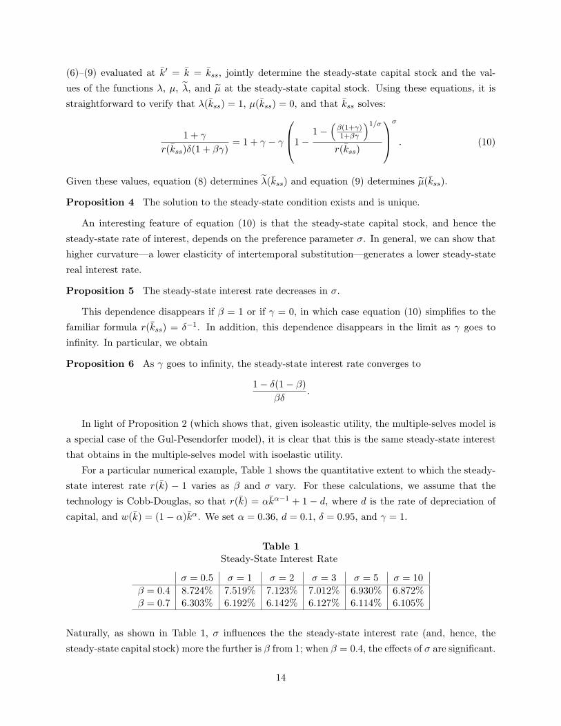
For a particular numerical example, Table 1 shows the quantitative extent to which the steady-

state interest rate r(k) − 1 varies as β and σ vary. For these calculations, we assume that the

technology is Cobb-Douglas, so that r(k) = αkα−1 + 1 − d, where d is the rate of depreciation of

capital, and w(k) = (1− α)kα. We set α = 0.36, d = 0.1, δ = 0.95, and γ = 1.

Table 1Steady-State Interest Rate

σ = 0.5 σ = 1 σ = 2 σ = 3 σ = 5 σ = 10β = 0.4 8.724% 7.519% 7.123% 7.012% 6.930% 6.872%β = 0.7 6.303% 6.192% 6.142% 6.127% 6.114% 6.105%

Naturally, as shown in Table 1, σ influences the the steady-state interest rate (and, hence, the

steady-state capital stock) more the further is β from 1; when β = 0.4, the effects of σ are significant.

14

Intuitively, the reason why steady-state savings increase in σ is that more curvature makes a given

amount of current saving decrease the future self-control cost more. Consider a given c and c,

where c > c because the temptation is to consume more. The first-order condition (4) for actual

consumption shows that there is an “extra” return from more wealth next period in this model.

It is the effect on the self-control term in utility, γ (u(c)− u(c)) < 0, from a marginal increase in

wealth: γ (u′(c)− u′(c)) > 0. This amount is higher, the more curvature there is: the more curved

is utility, the higher is u′(c) relative to u′(c). Thus, with a higher extra return from saving, the

steady-state capital stock will rise.

Needless to say, the determination of the steady state is more complex in this model than in

the standard model. Moreover, without isoelastic utility, we do not know how to find steady states

without simultaneously solving for the decision rules globally.

Dynamics. Global dynamics can be characterized numerically, though it is somewhat more cum-

bersome than in the corresponding standard model. In Appendix 2, we explain in detail the nu-

merical procedures that we used.

For a particular example, Table 2 illustrates how the local speed of convergence to the steady

state (i.e., the quantity λ′(kss)kss + λ(kss) + µ′(kss)) varies as σ and β vary, holding the steady

state constant. For these calculations, we assume, as we did in the section on steady states, that

the technology is Cobb-Douglas. We set α = 0.36, d = 0.1, and γ = 1; for each pair (σ, β), we

choose δ so that the steady-state interest rate is the one that prevails when β = 1 and δ = 0.95

(recall that when β = 1, the steady-state interest rate does not depend on σ).

Table 2Speed of Adjustment to the Steady State

β = 0.25 β = 0.5 β = 0.75 β = 1σ = 0.5 0.79093 0.79757 0.80155 0.80477σ = 1 0.86039 0.86039 0.86039 0.86039σ = 3 0.93254 0.93075 0.92854 0.92643

Table 2 shows that, holding the interest rate fixed, the (local) speed of convergence to the steady

state increases as β increases and as σ increases. Because the interest rate is fixed in Table 2, these

results indicate that the model in which temptation and self-control play a role is not observationally

equivalent to the standard model (i.e., the one that obtains when β = 1), except in the special case

that σ = 1, i.e., the case of logarithmic utility (recall Proposition 3 on observational equivalence to

the standard model when σ = 1).

Two special cases. We consider two particular cases for illustration. First, when β = 0, one can

show that λ(k) = 0 and µ(k) = −w(k)/(r(k)− 1): the temptation is to consume all present-value

15

wealth. In this case, equation (10), which determines the steady-state interest rate, simplifies to:

1δr(kss)

= 1− γ

1 + γ

(r(kss)

r(kss)− 1

)−σ

.

Hence, even when β = 0, the steady-state interest rate depends on the preference parameter σ.

Second, we consider the log-Cobb model: logarithmic u, full depreciation, and Cobb-Douglas

production (i.e., f(k) = Akα, 0 < α < 1). Under these parametric restrictions, we can completely

characterize the competitive equilibrium by means of analytical expressions for the decision rules.

Specifically,

W (k, k) = A0 + A1 log(k) + A2 log(k + ϕk),

where A0, A1, A2, and ϕ are undetermined coefficients that can be computed using a standard

guess-and-verify method.11 Since u is isoelastic, the “realized” decision rule has the same form as

above, with

λ(k) =δ

δ + (1− δ) 1+γ1+βγ

r(k)

and µ(k) = 0, implying that

G(k) = g(k, k) =αδ

δ + (1− δ) 1+γ1+βγ

Akα.

The “temptation” decision rule also has the same form as above, with

λ(k) =δβ

1− δ + δβr(k)

and

µ(k) =δβ

1− δ + δβw(k)− ϕ(1− δ)

1− δ + δβG(k).

If γ = 0 or β = 1, then we have the standard model: the savings rate out of current output is αδ.

If γ > 0 and β < 1 (i.e., if there are self-control problems), then the savings rate falls relative to

the standard model.

3 Policy

In this section, we turn to normative analysis. The general idea here is not to show how temptation

and self-control problems can be completely overcome, but rather to discuss the potential of simple

policies to improve on laissez-faire allocations. In general, in these environments, consumers would

benefit from commitment, so to the extent this can be “given” to them, welfare must rise, and indeed

all temptation (and, obviously, self-control) problems will be overcome. Thus, we focus instead on

commonly used tax/transfer policy: we look at the effects of (constant) proportional taxes and

subsidies. Thus, let there be a proportional tax (or subsidy) τi on savings every period; we consider

a time-independent tax rate for simplicity mainly.12 In addition to the proportional tax, there is11In particular, A1 = α−1

(1−δ)(1−αδ)A2 = 1

1−δ, and ϕ = 1−α

α(1−δ)(1+γ)+δ(1+βγ)

(1−δ)(1+γ).

12For some of the environments below, a time-independent tax rate will be optimal in the class of all proportional(and possibly time-dependent) tax rules, but this is not a general result.

16

a lump-sum transfer (or tax) Υ, which can be levied once or in installments at different points in

time; due to the assumption of perfect capital markets (i.e., there not being liquidity/borrowing

constraints) the timing is irrelevant.

As shown in Krusell, Kuruscu, and Smith (2009), the restriction to a constant tax rate does

not bind when utility is logarithmic: in this case, when the government has full commitment to a

possibly time-varying sequence of taxes, it chooses a constant tax (or subsidy) when the planning

horizon is infinitely long.

3.1 Equilibrium with taxes

We allow for less than full depreciation. We assume that the government taxes capital income (net

of depreciation) at a constant rate τk and labor income at a constant rate τl . In addition, the

government subsidizes capital carried into the next period at constant rate τi. The government

balances its budget in each period. A typical consumer’s problem then takes the following recursive

form:

W (k, k) = maxk′

{(1 + γ)u

((1 + (f ′(k)− d)(1− τk))k + w(k)(1− τl)− (1 + τi)k′

)+ δ(1 + βγ)W (k′, k′)

}−

γ maxk′

{u((1 + (f ′(k)− d)(1− τk))k + w(k)(1− τl)− (1 + τi)k′

)+ βδW (k′, k′)

}.

The consumer takes as given a law of motion k′ = G(k) for aggregate capital; the pricing functions

r(k) and w(k) are determined by the first-order conditions to the firm’s static profit-maximization

problem. The consumer also takes into account the government’s budget constraint:

(f ′(k)− d)kτk + w(k)τl = −τik′.

Specifically, we let the government choose a time-invariant subsidy rate τi; the government’s

budget constraint then places a restriction on the two tax rates τk and τl. As in Section 2.3.2, the

consumer’s problem determines a “realized” decision rule g(k, k) which solves the first maximization

problem and a “temptation” decision rule g(k, k) which solves the second maximization problem.

In equilibrium, we require g(k, k) = G(k).

3.2 Solving the model

For the case of isoelastic utility, we could solve this problem using the results of Proposition 1 in

Section 2.3.2. In this section, however, we are interested not only in equilibrium behavior but also

in consumer welfare, so we solve directly for the consumer’s value function. If u is logarithmic, one

can use a guess-and-verify approach to show that the consumer’s value function takes the form

W (k, k) = a(k) + (1− δ)−1 log(k + b(k)),

17

where the functions a and b satisfy a pair of functional equations

a(k) = A(δ, β, γ, τi) + (1− δ)−1 log(1 + (f ′(k)− d)(1− τk)

)+ δa(k′) (11)

b(k) =w(k)(1− τl) + (1 + τi)b(k′)

1 + (f ′(k)− d)(1− τk), (12)

where A(δ, β, γ, τi) is a complicated function of the parameters δ, β, γ, and τi.13 The consumer’s

decision rule is then given by

k′ =δ(1 + βγ)(1− δ)−1

[(1 + (f ′(k)− d)(1− τk)

)k + w(k)(1− τl)

](1 + γ + δ(1 + βγ)(1− δ)−1)(1 + τi)

−

(1 + γ)b(k′)1 + γ + δ(1 + βγ)(1− δ)−1

. (13)

To obtain the aggregate law of motion k′ = G(k), impose the equilibrium conditions k = k and

k′ = k′ in the consumer’s decision rule.

For the quantitative results reported below, we use a common tax rate for capital and labor

income: that is, we set τk = τl = τy. In this case, the government budget constraint can be used to

express τy as a function of k, k′, and τi. This expression can be substituted into equations (12) and

(13) to eliminate τk and τl. Finally, because we want to study welfare as the economy transits from

a steady state without taxation to a steady state with taxation, we need to solve for an equilibrium

globally. To do so, it is necessary in the calibrated model to solve the model numerically. We

describe the methods we used in Appendix 3.

3.3 Calibration

Some of the calibration follows the existing, standard literature.

3.3.1 The standard part

In the quantitative analysis of optimal policy, several of the preference and technology parameter

values are the same as in Section 2.3.2. We experimented with different intertemporal elasticities,

but it turns out that the results are rather robust in this dimension; the results below therefore

only refer to the case where u is logarithmic. The discount rate δ is set to 0.95 in our benchmark

but we also varied it along with the variations in β and γ so as to maintain a constant steady-state

interest rate. However, whether δ is adjusted in this manner or not also has very little effect on the

results, so we only report the cases where it is fixed. The rate of depreciation d is set to 0.1 and

the technology is Cobb-Douglas with capital’s share equal to 0.36.13For the case of isoelastic utility with elasticity σ−1, the value function takes the form

W (k, k) = (1− δ)−1a(k)(k + b(k))1−σ,

where the functions a and b satisfy a pair of functional equations analogous to equations (11) and (12).

18

3.3.2 Temptation and self-control

We consider a range of different values for the two “temptation” parameters β (which determines the

nature of the temptation) and γ (which determines the strength of the temptation). To provide some

guidance in how to interpret the various values of β and γ, we imagine asking a typical consumer to

answer two hypothetical questions.14 First, how much better off would you be if you were relieved

of self-control problems but were not allowed to vary your allocation from the equilibrium one?

Second, how much better off would you be if you were relieved of self-control problems and could

then choose a new allocation given that all other consumers’ allocations remain at the equilibrium

one? In other words, if the government were to pick a command policy outcome for you (while still

respecting your budget constraint), how much better off would you be?15

To answer the first question, we set γ = 0, evaluate welfare given the equilibrium allocation,

and then ask how much consumption (as a percentage in each period) the consumer would be

willing to give up in order to make him just as well off as he in the equilibrium with self-control

problems. To answer the second question, we set γ = 0, solve the (small) consumer’s problem given

the equilibrium behavior of prices, evaluate welfare given the consumer’s revised choices, and then

compute a percentage consumption equivalent as for the first question.

Clearly, the consumer prefers the second scenario over the first one. In the multiple-selves

model (in which γ goes to infinity), the answer to the first question is 0, since in equilibrium the

consumer succumbs completely to his temptation and, consequently, does not experience a utility

cost of self-control. In this case, however, the welfare benefits to choosing a new allocation in the

absence of self-control problems can be quite large, so that the gap between the answers to the two

questions is also large. At the other extreme, as we show below, by choosing β and γ appropriately,

the cost of self-control can be large and yet the additional benefit of choosing a new allocation in

the absence of self-control problems can be small.

3.4 Quantitative results

Each panel in Table 3 corresponds to one value of the self-control cost, as assessed by the consumer’s

answer to Q#1, and the different rows in each panel vary the cost of not having commitment, as

assessed by the consumer’s answer to Q#2.16 For each combination of these two costs, the (β, γ)

pair that leads a steady-state consumer to give these answers is listed.17

14The use of hypothetical questions is not new; it is, for example, one of the main tools for eliciting consumers’attitudes toward risk, and answers to such questions have thus been used to parameterize risk aversion.

15Note that these questions do not pin down the direction of temptation, i.e., whether β < 1 or whether actuallyβ > 1, a case considered in Krusell, Kuruscu, Smith (2002b). However, we presume that the former is the relevantcase.

16The self-control costs are reported as percentages of consumption per period (i.e., 0.1 means one-tenth of onepercent).

17To be precise, each (β, γ) pair is chosen to match given values for the answer to Q#1 and for the value of ∆,which is approximately equal to the difference between the answers to Q#1 and Q#2 (see the definition of ∆ in thenotes to Table 3).

19

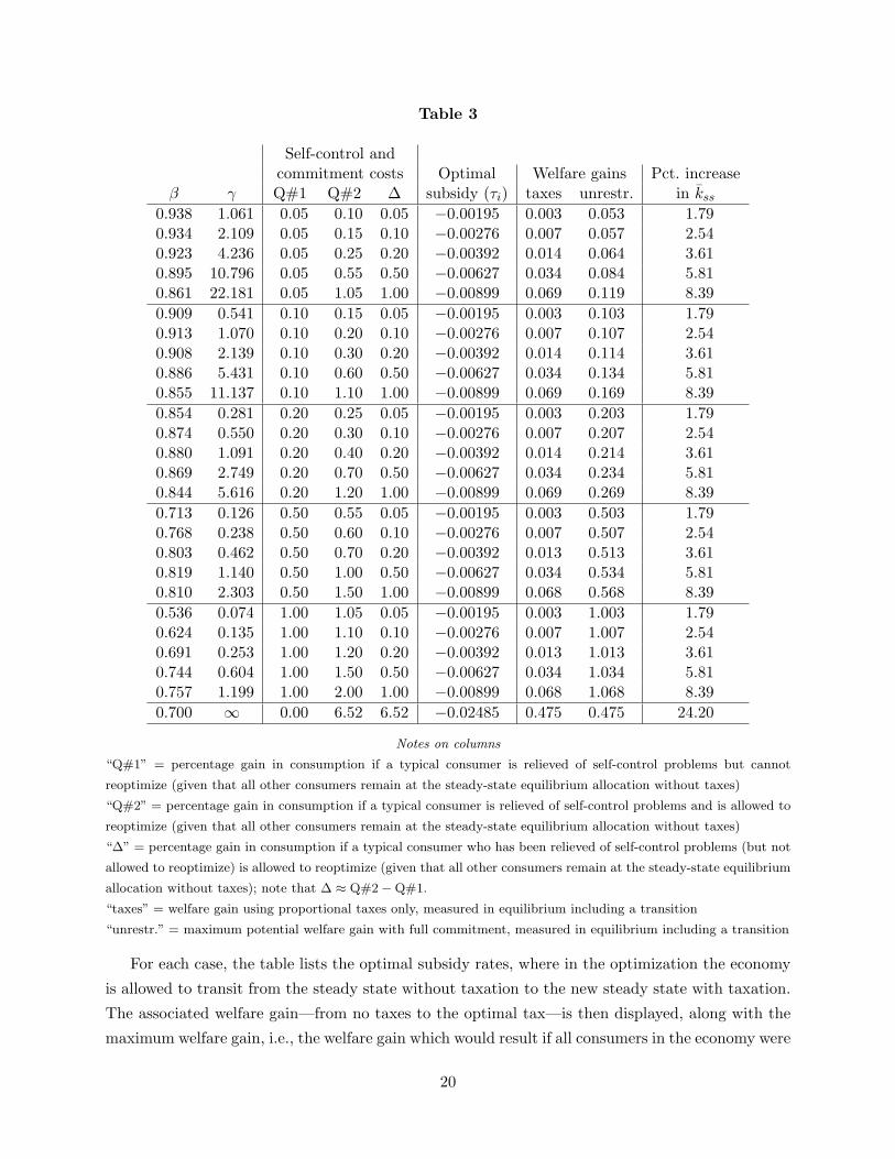
Table 3

Self-control andcommitment costs Optimal Welfare gains Pct. increase

β γ Q#1 Q#2 ∆ subsidy (τi) taxes unrestr. in kss

0.938 1.061 0.05 0.10 0.05 −0.00195 0.003 0.053 1.790.934 2.109 0.05 0.15 0.10 −0.00276 0.007 0.057 2.540.923 4.236 0.05 0.25 0.20 −0.00392 0.014 0.064 3.610.895 10.796 0.05 0.55 0.50 −0.00627 0.034 0.084 5.810.861 22.181 0.05 1.05 1.00 −0.00899 0.069 0.119 8.390.909 0.541 0.10 0.15 0.05 −0.00195 0.003 0.103 1.790.913 1.070 0.10 0.20 0.10 −0.00276 0.007 0.107 2.540.908 2.139 0.10 0.30 0.20 −0.00392 0.014 0.114 3.610.886 5.431 0.10 0.60 0.50 −0.00627 0.034 0.134 5.810.855 11.137 0.10 1.10 1.00 −0.00899 0.069 0.169 8.390.854 0.281 0.20 0.25 0.05 −0.00195 0.003 0.203 1.790.874 0.550 0.20 0.30 0.10 −0.00276 0.007 0.207 2.540.880 1.091 0.20 0.40 0.20 −0.00392 0.014 0.214 3.610.869 2.749 0.20 0.70 0.50 −0.00627 0.034 0.234 5.810.844 5.616 0.20 1.20 1.00 −0.00899 0.069 0.269 8.390.713 0.126 0.50 0.55 0.05 −0.00195 0.003 0.503 1.790.768 0.238 0.50 0.60 0.10 −0.00276 0.007 0.507 2.540.803 0.462 0.50 0.70 0.20 −0.00392 0.013 0.513 3.610.819 1.140 0.50 1.00 0.50 −0.00627 0.034 0.534 5.810.810 2.303 0.50 1.50 1.00 −0.00899 0.068 0.568 8.390.536 0.074 1.00 1.05 0.05 −0.00195 0.003 1.003 1.790.624 0.135 1.00 1.10 0.10 −0.00276 0.007 1.007 2.540.691 0.253 1.00 1.20 0.20 −0.00392 0.013 1.013 3.610.744 0.604 1.00 1.50 0.50 −0.00627 0.034 1.034 5.810.757 1.199 1.00 2.00 1.00 −0.00899 0.068 1.068 8.390.700 ∞ 0.00 6.52 6.52 −0.02485 0.475 0.475 24.20

Notes on columns

“Q#1” = percentage gain in consumption if a typical consumer is relieved of self-control problems but cannot

reoptimize (given that all other consumers remain at the steady-state equilibrium allocation without taxes)

“Q#2” = percentage gain in consumption if a typical consumer is relieved of self-control problems and is allowed to

reoptimize (given that all other consumers remain at the steady-state equilibrium allocation without taxes)

“∆” = percentage gain in consumption if a typical consumer who has been relieved of self-control problems (but not

allowed to reoptimize) is allowed to reoptimize (given that all other consumers remain at the steady-state equilibrium

allocation without taxes); note that ∆ ≈ Q#2−Q#1.

“taxes” = welfare gain using proportional taxes only, measured in equilibrium including a transition

“unrestr.” = maximum potential welfare gain with full commitment, measured in equilibrium including a transition

For each case, the table lists the optimal subsidy rates, where in the optimization the economy

is allowed to transit from the steady state without taxation to the new steady state with taxation.

The associated welfare gain—from no taxes to the optimal tax—is then displayed, along with the

maximum welfare gain, i.e., the welfare gain which would result if all consumers in the economy were

20

given access to commitment and were allowed to reoptimize (the maximum gain can be computed

by simply setting γ to 0 and solving for the transition).18 Finally, the last column in the table

shows the percentage increase in the long-run capital stock that results from the optimal subsidy.

In terms of our substantive results, first, it appears that the optimal subsidy rates are, at first

glance, quite small, even when self-control costs are reasonably large. Notice, however, that the

gross after-tax return to capital,

R(k) ≡ 1 + (f ′(k)− d)(1− τk)1 + τi

,

is approximately (for τk small) equal to 1 + f ′(k) − d − τi. Thus the gross after-tax return to

capital increases one for one (approximately) with the investment subsidy rate, so the numbers in

the table translate roughly to changes in the before-tax interest rate of between 20 and 90 basis

points. Because, in a steady state, the after-tax return to capital is pinned down by the preference

parameters β, δ, γ, and σ (see equation (10), with R(kss) in place of r(kss)), an increase in the

subsidy leads to an increase in the steady-state capital stock (so that the marginal product of

capital r(k) is driven down). As reported in Table 3, the percentage increase in the steady-state

capital stock induced by the optimal subsidy can be quite substantial, as large as 8% when the

difference between the two measures of the self-control cost is 1%.

Second, the optimal subsidy appears to depend solely on the difference ∆ between the two

measures of the cost of self-control. In the two-period model with logarithmic period utility (see

Sections 3.2 and 3.3), we can prove (holding δ fixed as it is in Table 3) that this is an exact result.19

Our quantitative results suggest that such a result holds for the long-horizon model, too. The

table also reveals that both the percentage increase in the steady-state capital stock induced by the

optimal subsidy and the welfare gain associated with the optimal subsidy depend nearly exactly

on the difference ∆.20

18The welfare measures in the table are expressed using the typical “percentage consumption equivalent”, butnotice that such a measure has to be computed with care in this model, because when consumption is shifted up ordown by some percentage points, one needs to specify what happens to the choice set. To avoid this ambiguity, wetherefore always perform the scaling of consumption in an alternative with full commitment, where the choice set isimmaterial. Hence, “0.05” in the third column means that the consumer is indifferent between the given steady-statesituation and an alternative with a 0.05% lower consumption allocation at all dates but no choice; similarly, “1.00” inthe fourth column means that there is indifference between the steady-state situation and an alternative which allowsfull commitment but is scaled down by 1.00%. The maximum welfare gains (the eighth column) similarly states thenumber, say, 0.014, such that the consumer is indifferent between the steady-state situation and a new equilibriumwhere all consumers have full commitment but lower consumption by 0.014 percent. The welfare gains under optimaltaxes, finally, is more complicated: it is computed as the difference between the similar equivalent consumption gainof moving from the steady-state situation to one with full commitment and the equivalent consumption gain frommoving from the optimal-tax equilibrium to one with full commitment.

19In particular, one can show (we omit the proof for brevity) that:

log(1 + ∆) =1

1 + δ

[log

(1

1 + δ(1 + τi)

)+ δ log

(δ(1 + τi)

1 + δ(1 + τi)

)− log

(1

1 + δ

)− δ log

(δ

1 + δ

)].

20Again, for the two-period model with log utility, we can prove that these results are exact. Our quantitativeresults suggest that this exactness holds with a long horizon, too, provided that period utility is logarithmic.

21

To interpret this second set of findings, note that the difference between the two measures of

the self-control cost captures the extent to which reoptimizing, over and above being relieved of the

utility cost of self-control, benefits the consumer. Because one of the purposes of the subsidy is to

change consumers’ behavior, it seems sensible that the optimal subsidy depends on the extent to

which consumers gain from reoptimizing once they are relieved of their self-control problems. An

intuitive statement of these findings is thus that if the self-control problems are mainly of the variety

that leads consumers to succumb, or almost succumb—the way in which we interpret the multiple-

selves model—then government policy can be helpful because it does force different behavior. If,

on the other hand, temptation does not lead consumers to succumb but rather mainly to exercise

(costly) self-control, then government policy is very ineffective, since temptation problems largely

remain with the new tax policy.

Third, the welfare gains from the optimal subsidy are much lower than the answer to Q#2—our

individual-based, or partial-equilibrium assessment—would indicate. For example, in the multiple-

selves model the consumer would pay over 6% of consumption for commitment at given prices,

but if all consumers were given commitment, the ultimate welfare gain would only be a little less

than half of one percent.21 This is because the latter measure is an equilibrium measure: when

all consumers have commitment, savings rise significantly, thus lowering the return on savings.

Thus, price changes offset most of the effects of taxes. Here a comparison with an endowment

economy is helpful. As discussed in Section 2.5.1 in Krusell, Kuruscu, and Smith (2009), in an

endowment economy the entire individual gain is always wiped out by price changes in response

to the investment subsidy: net-of-tax prices cannot change in an endowment economy. Evidently,

though our production economy allows welfare gains from aggregate policy, these gains are small.22

Fourth, the table reveals that the welfare gain from complete commitment (column eight)

minus the welfare gain from optimal taxes (column seven) exactly equals the answer to Q#1.

To understand why, recall from Proposition 8 that in the two-period model with log utility, the

equilibrium allocation induced by the optimal subsidy is identical to the command allocation (i.e.,

the “first-best” allocation that is attained under full commitment). Our quantitative experiments

suggest that this result holds for the long-horizon model, too.23 Thus the difference between

columns eight and seven is a measure of self-control in the spirit of Q#1: the allocation does not

change but the consumer is relieved of his self-control problems. Moreover, under log utility the self-

control cost does not depend on prices.24 It follows then that the difference between columns eight

and seven must be equal to the answer to Q#1. These findings again support our general conclusion21Though the welfare gains from optimal policy are very different in partial and in general equilibrium, it turns

out in our examples that the optimal tax rates in these two cases are quite similar.22Also, notice that the maximum welfare gains are sometimes decreasing in γ—rows 5, 10, and 11—and sometimes

increasing in γ—rows 17 and 25. Thus, this is another feature shared with the endowment economy.23That a constant subsidy is sufficient for attaining the first-best allocation is a special result that obtains only

under logarithmic utility; with other assumptions on curvature, a time-dependent subsidy would be required.24One can show this by showing that with log utility a typical consumer’s realized consumption, as well as his

temptation consumption, can be expressed as constant fractions of lifetime resources (we omit the proof for brevity).

22

that optimal subsidies are effective at changing equilibrium behavior but not at alleviating the costs

of self-control: for the log case, this is, in fact, an exact result.

A special row in the table is the last row, which shows a special case where γ is infinity: the

multiple-selves model. Here, self-control costs are zero (Q#1), because the consumer succumbs.

Using logarithmic utility and fixing β at 0.7, which is a typical value in the studies of Laibson

and others, we thus find that consumers would gain about 6% in consumption terms if they were

allowed to reoptimize at given prices and that the optimal subsidy is a little over more than 2%.

In addition, the optimal subsidy achieves a first-best outcome in terms of welfare: the seventh and

eighth columns are the same. This result arises because, one, the optimal subsidy leads to the

first-best allocation and, two, the self-control cost is zero when γ is infinity. Again, this result is

special to the case of logarithmic curvature of period utility.

We have also computed results when the coefficient of relative risk aversion (σ) is equal to either

one-half or two, rather than one as in the log case. For these cases, the results described above no

longer hold exactly, but they continue to be valid approximately. For example, although the optimal

subsidy does not vary exactly with the difference ∆, the deviations from this exactness are not

quantitatively large. In addition, the difference between columns eight and seven is approximately,

but not exactly, equal to the answer Q#1. Consequently, the results for σ = 1/2 and σ = 2 are

qualitatively similar to the results reported in Table 3, which are for σ = 1. In addition, the

qualitative results do not change, and the quantitative results change only slightly, if the discount

rate δ is varied as β and γ are varied so as to keep the steady-state capital stock constant (prior to

changing taxes).

Finally, the table also illustrates that the mapping from our measures of self-control and com-

mitment costs—the answers to Q#1 and Q#2—to (β, γ) is quite nontrivial. Comparing across

panels, a higher self-control cost (Q#1) is associated with lower β’s but also with lower γ’s over

some range. Similarly, a higher commitment cost within any panel (Q#2) is associated with higher

γ’s but either higher β’s or lower β’s.

4 Conclusion

In this paper, we have developed a version of the consumer preference specification advanced by

Gul and Pesendorfer (2001, 2004) that is suitable for dynamic macroeconomic analysis, and we have

applied it in order to analyze the role of proportional taxes for consumer welfare. Our dynamic

extension to the Gul-Pesendorfer specification of temptation and self-control involves what we refer

to as quasi-geometric temptation. As a special case—when the disutility of self control becomes very

strong, as measured by our parameter γ approaching infinity—this setting delivers the multiple-

selves model, here in a setting that makes clear how to use it to conduct normative experiments.

In developing the theory, we maintained the standard assumptions for the curvature of preferences,

and we showed that these assumptions allow aggregation in wealth as well as tractable steady-

23

state analysis. We also proposed some intuitive measures that are useful in the calibration of

temptation and self-control preferences. Finally, we demonstrated how the model can be analyzed

with numerical methods.

Are proportional taxes a useful instrument for improving consumer welfare under the alterna-

tive view of consumer preferences maintained here? Though not self-evident, we found that in

the context of a simple two-period model, the answer is yes: under quite general assumptions, the

government should subsidize investment. For our fully dynamic model, we also made a quantita-

tive assessment, concluding that the benefits from investment subsidies are positive there as well.

However, they are rather small, especially if the temptation and self-control problems of consumers

are associated with the costly exercise of self-control (choose a salad over the hamburger but suffer

in the process). When consumers’ preferences are such that they succumb (choose the hamburger,

which gives lower utility than choosing a salad from a menu which does not offer hamburgers),

government policy is somewhat more helpful. In addition, we found that the general-equilibrium

effects of tax policy can differ substantively from the partial-equilibrium effects, which is another

important reason for our findings that the potential welfare gains from investment subsidies are

small.

The focus on proportional taxes and subsidies is clearly restrictive; nonlinear instruments can

be productively used when consumers’ preferences feature temptation and self-control problems.

In particular, an outside agent (such as a government or another private agent or organization)

could offer to “restrict” the given consumer’s choices appropriately and increase welfare as a result.

Depending on the choice problem, this restriction would need to be more or less elaborate. For

example, in the context of a consumption-savings problem, a requirement that savings do not

fall below some preset level might suffice; interestingly, such a policy cannot be improved upon

even when there is also a need for “flexibility”, as defined and analyzed in Amador, Werning, and

Angeletos (2003). The market structure matters for welfare as well. First, it is not too difficult to

see, in a two-period model, that the consumer is better off in “autarky” (i.e., in an environment

without markets in which each consumer operates his own “backyard” technology) than in a setting

with competitive trade.25 Second, Kocherlakota (2001), Ludmer (2004), and Krusell and Ludmer

(2006) illustrate how the addition of various asset markets can either lead to an increase or a decrease

in welfare. Collectively, these analyses help us understand the mechanisms whereby different policies

and regulations influence welfare. For future research, it would be important to develop theory that

allows us to understand when and why commitment mechanisms are available, either individually25Although the competitive equilibrium and autarky allocations coincide in the two-period model, the temptation

is weaker in autarky, implying that the disutility of self-control is smaller. The temptation is weaker in autarkybecause the production possibilities frontier (which plays the role of the consumer’s “budget constraint” in autarky)lies strictly inside the (triangular) budget set faced by a consumer in competitive equilibrium. In other words, theutility that the consumer could gain by succumbing to the temptation is larger under competitive equilibrium than inautarky. Since the allocations are identical, the consumer must exert more self-control (i.e., incur a larger disutility ofself-control) under competitive equilibrium than in autarky. Consequently, the consumer is worse off in competitiveequilibrium than in autarky, even though the outcomes are the same!

24

by consumers or within groups of individuals. For actual policy recommendations, one would

especially need to take consumer heterogeneity into account, both in terms of possible differences

in preferences and in economic conditions (such as wealth and earnings ability).

25

References

[1] Akerlof, George A. (1991), “Procrastination and Obedience”, American Economic Review 81,1–19.

[2] Amador, Manuel, Ivan Werning, and George-Marios Angeletos (2003), “Commitment vs. Flex-ibility”, NBER working paper #10151.

[3] Angeletos, George-Marios, David Laibson, Andrea Repetto, Jeremy Tobacman, and StephenWeinberg (2001), “The Hyperbolic Consumption Model: Calibration, Simulation, and Empir-ical Evaluation”, Journal of Economic Perspectives 15, 47–68.

[4] Barro, Robert (1999), “Ramsey Meets Laibson in the Neoclassical Growth Model”, QuarterlyJournal of Economics 114, 1125–1152.

[5] Bernheim, Douglas B., Debraj Ray, and Sevin Yeltekin (1999), “Self-Control, Saving, and theLow Asset Trap”, manuscript.

[6] Esteban, Susanna and Eiichi Miyagawa (2003), “Nonlinear Pricing with Self-Control Prefer-ences”, working paper.

[7] Esteban, Susanna and Eiichi Miyagawa (2004), “Optimal Menu of Menus with Self-ControlPreferences”, working paper.

[8] Gul, Faruk and Wolfgang Pesendorfer (2001), “Temptation and Self-Control”, Econometrica69, 1403–1435.

[9] Gul, Faruk and Wolfgang Pesendorfer (2004), “Self-Control and the Theory of Consumption”,Econometrica 72, 119–158.

[10] Gul, Faruk and Wolfgang Pesendorfer (2005), “The Revealed Preference Theory of ChangingTastes,” Review of Economic Studies 72, 429–448.

[11] Hercowitz, Zvi and Per Krusell (2000), “Overheating?”, manuscript.

[12] Kocherlakota, Narayana (2001), “Looking for Evidence of Time-Inconsistent Preference inAsset Market Data”, Federal Reserve Bank of Minneapolis Quarterly Review 25:3, 13–24.

[13] Krusell, Per, Burhanettin Kuruscu, and Anthony A. Smith, Jr. (2000), “Tax Policy withQuasi-Geometric Discounting”, International Economic Journal , Vol. 14, No:3, pp:1-40.

[14] Krusell, Per, Burhanettin Kuruscu, and Anthony A. Smith, Jr. (2002a), “Equilibrium Welfareand Government Policy with Quasi-Geometric Discounting”, Journal of Economic Theory,105, 42–72.

[15] Krusell, Per, Burhanettin Kuruscu, and Anthony A. Smith, Jr. (2002b), “Time Orientationand Asset Prices”, Journal of Monetary Economics, 49, 107–135.

[16] Krusell, Per, Burhanettin Kuruscu, and Anthony A. Smith, Jr. (2009), “Temptation andTaxation”, working paper.

26

[17] Krusell, Per and Sebastian Ludmer (2006), “Self-Control, Markets, and Aggregate Savings,”working paper.

[18] Krusell, Per and Anthony A. Smith, Jr. (2003), “Consumption-Savings Decisions with Quasi-Geometric Discounting”, Econometrica 71, 365–375.

[19] Laibson, David (1994), “Self-Control and Saving”, manuscript.

[20] Laibson, David (1996), “Hyperbolic Discount Functions, Undersaving, and Savings Policy”,NBER Working Paper 5635.

[21] Laibson, David (1997), “Hyperbolic Discount Functions and Time Preference Heterogeneity”,manuscript.

[22] Laibson, David, Andrea Repeto, and Jeremy Tobacman (2004), “Estimating Discount Func-tions from Lifecycle Consumption Choices”, working paper.

[23] Ludmer, Sebastian (2004), “Self-control and Illiquid Assets,” working paper.

[24] Noor, Jawwad (2005), “Temptation, Welfare and Revealed Preference”, working paper.

[25] O’Donoghue, Edward D. and Matthew Rabin (1999), “Doing It Now or Doing It Later”,American Economic Review 89, 103–124.

[26] Phelps, Edmund S. and Robert A. Pollak (1968), “On Second-best National Saving and Game-equilibrium Growth”, Review of Economic Studies 35, 185–199.

[27] Schelling, Thomas (1984), “Self-Command in Practice, in Policy, and in a Theory of RationalChoice”, American Economic Review 74, 1–11.

[28] Strotz, Robert H. (1956), “Myopia and Inconsistency in Dynamic Utility Maximization”, Re-view of Economic Studies 23, 165–180.

27

Appendix 1

This appendix provides the proofs of Propositions 1–8.

Proof of Proposition 1: The two Euler equations are:

(1 + γ)u′(r(k)k + w(k)− g(k, k)) =

δ(1 + βγ)r(g(k, k))((1 + γ)u′(r(g(k, k))g(k, k) + w(g(k, k))− g(g(k, k), g(k, k)))−

γu′(r(g(k, k))g(k, k) + w(g(k, k))− g(g(k, k), g(k, k))))

andu′(r(k)k + w(k)− g(k, k)) =

δβr(g(k, k))((1 + γ)u′(r(g(k, k))g(k, k) + w(g(k, k))− g(g(k, k), g(k, k)))

−γu′(r(g(k, k))g(k, k) + w(g(k, k))− g(g(k, k), g(k, k)))).

Inserting the guesses for g(k, k) and g(k, k) into these equations and using the fact that u isisoelastic, we obtain:

(1 + γ)δ(1 + βγ)r(g(k, k))

=

(1 + γ)

(r(k′)− λ(k′))λ(k)r(k)− λ(k)

k + µ(k)

λ(k)+ w(k′)−µ(k′)

(r(k′)−λ(k′))λ(k)

k + w(k)−µ(k)

r(k)−λ(k)

−σ

−γ

(r(k′)− λ(k′))λ(k)r(k)− λ(k)

k + µ(k)

λ(k)+ w(k′)−µ(k′)

(r(k′)−λ(k′))λ(k)

k + w(k)−µ(k)

r(k)−λ(k)

−σ

1δβr(g(k, k))

=

(1 + γ)

(r(k′)− λ(k′))λ(k)r(k)− λ(k)

k + µ(k)

λ(k)+ w(k′)−µ(k′)

(r(k′)−λ(k′))λ(k)

k + w(k)−µ(k)

r(k)−λ(k)

−σ

−γ

(r(k′)− λ(k′))λ(k)r(k)− λ(k)

k + µ(k)

λ(k)+ w(k′)−µ(k′)

(r(k′)−λ(k′))λ(k)

k + w(k)−µ(k)

r(k)−λ(k)

−σ

Note that these two Euler equations must hold for all k. This implies that:

µ(k)λ(k)

+w(k′)− µ(k′)

(r(k′)− λ(k′))λ(k)=

w(k)− µ(k)r(k)− λ(k)

(14)

µ(k)λ(k)

+w(k′)− µ(k′)

(r(k′)− λ(k′))λ(k)=

w(k)− µ(k)r(k)− λ(k)

(15)

µ(k)λ(k)

+w(k′)− µ(k′)

(r(k′)− λ(k′))λ(k)=

w(k)− µ(k)r(k)− λ(k)

(16)

28

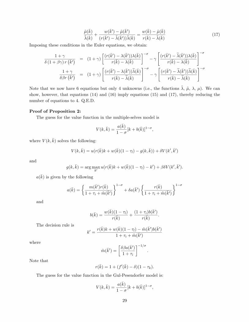
µ(k)λ(k)

+w(k′)− µ(k′)

(r(k′)− λ(k′))λ(k)=

w(k)− µ(k)r(k)− λ(k)

(17)

Imposing these conditions in the Euler equations, we obtain:

1 + γ

δ (1 + βγ) r(k′) = (1 + γ)

[(r(k′)− λ(k′))λ(k)

r(k)− λ(k)

]−σ

− γ

[(r(k′)− λ(k′))λ(k)

r(k)− λ(k)

]−σ

1 + γ

δβr(k′) = (1 + γ)

[(r(k′)− λ(k′))λ(k)

r(k)− λ(k)

]−σ

− γ

[(r(k′)− λ(k′))λ(k)

r(k)− λ(k)

]−σ

Note that we now have 6 equations but only 4 unknowns (i.e., the functions λ, µ, λ, µ). We canshow, however, that equations (14) and (16) imply equations (15) and (17), thereby reducing thenumber of equations to 4. Q.E.D.

Proof of Proposition 2:The guess for the value function in the multiple-selves model is

V (k, k) =a(k)1− σ

[k + b(k)]1−σ,

where V (k, k) solves the following:

V (k, k) = u(r(k)k + w(k)(1− τl)− g(k, k)) + δV (k′, k′)

andg(k, k) = arg max

k′u(r(k)k + w(k)(1− τl)− k′) + βδV (k′, k′).

a(k) is given by the following

a(k) ={

m(k′)r(k)1 + τi + m(k′)

}1−σ

+ δa(k′){

r(k)1 + τi + m(k′)

}1−σ

and

b(k) =w(k)(1− τl)

r(k)+

(1 + τi)b(k′)r(k)

.

The decision rule is

k′ =r(k)k + w(k)(1− τl)− m(k′)b(k′)

1 + τi + m(k′)

where

m(k′) =[δβa(k′)1 + τi

]−1/σ

.

Note thatr(k) = 1 + (f ′(k)− δ)(1− τk).

The guess for the value function in the Gul-Pesendorfer model is:

V (k, k) =a(k)1− σ

[k + b(k)]1−σ,

29

where

b(k) =w(k)(1− τl)

r(k)+

(1 + τi)b(k′)r(k)

(18)

a(k) = (1 + γ){

m(k′)r(k)1 + τi + m(k′)

}1−σ

+ δ(1 + βγ)a(k′){

r(k)1 + τi + m(k′)

}1−σ

(19)

−γ

{m(k′)r(k)

1 + τi + m(k′)

}1−σ

− δβγa(k′){

r(k)1 + τi + m(k′)

}1−σ

m(k′) =[δ(1 + βγ)a(k′)(1 + γ)(1 + τi)

]−1/σ

m(k′) =[δβa(k′)1 + τi

]−1/σ

We can get k′ from the following equation:

k′ =r(k)k + w(k)(1− τl)−m(k′)b(k′)

1 + τi + m(k′).

We also have the temptation decision rule:

k′ =r(k)k + w(k)(1− τl)− m(k′)b(k′)

1 + τi + m(k′).

Comparing the Gul-Pesendorfer model and the multiple-selves model, one can see that thedecision rule and the value functions V (k, k) in the Gul-Pesendorfer model would converge to thedecision rule and the value function of the multiple-selves model if the equation that determinea(k) would converge to the corresponding equation in the multiple selves model. We can show thatthat will be true as γ goes to infinity.

Using somewhat less cumbersome notation, we need to show that

γ

{{m

1 + τ + m

}1−σ

−{

m

1 + τ + m

}1−σ}

+γδβa

{{1

1 + τ + m

}1−σ

−{

11 + τ + m

}1−σ}

goes to zero as γ goes to infinity, when

m = m

[1 + βγ

β + βγ

]− 1σ

≡ mr(γ)

and

m =[

δβa

1 + τ

]−1/σ

Now notice that the expression above can be written(1

1 + τ + m

)1−σ

γf(γ),

30

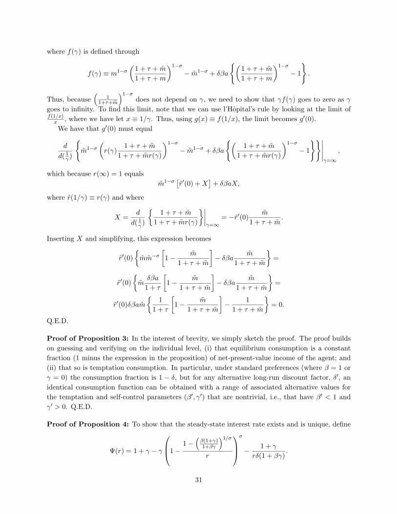
where f(γ) is defined through

f(γ) ≡ m1−σ

(1 + τ + m

1 + τ + m

)1−σ

− m1−σ + δβa

{(1 + τ + m

1 + τ + m

)1−σ

− 1

}.

Thus, because(

11+τ+m

)1−σdoes not depend on γ, we need to show that γf(γ) goes to zero as γ

goes to infinity. To find this limit, note that we can use l’Hopital’s rule by looking at the limit off(1/x)

x , where we have let x ≡ 1/γ. Thus, using g(x) ≡ f(1/x), the limit becomes g′(0).We have that g′(0) must equal

d

d( 1γ )

{m1−σ

(r(γ)

1 + τ + m

1 + τ + mr(γ)

)1−σ

− m1−σ + δβa

{(1 + τ + m

1 + τ + mr(γ)

)1−σ

− 1

}}∣∣∣∣∣γ=∞

,

which because r(∞) = 1 equalsm1−σ

[r′(0) + X

]+ δβaX,

where r(1/γ) ≡ r(γ) and where

X =d

d( 1γ )

{1 + τ + m

1 + τ + mr(γ)

}∣∣∣∣γ=∞

= −r′(0)m

1 + τ + m.

Inserting X and simplifying, this expression becomes

r′(0){

mm−σ

[1− m

1 + τ + m

]− δβa

m

1 + τ + m

}=

r′(0){

mδβa

1 + τ

[1− m

1 + τ + m

]− δβa

m

1 + τ + m

}=

r′(0)δβam

{1

1 + τ

[1− m

1 + τ + m

]− 1

1 + τ + m

}= 0.

Q.E.D.

Proof of Proposition 3: In the interest of brevity, we simply sketch the proof. The proof buildson guessing and verifying on the individual level, (i) that equilibrium consumption is a constantfraction (1 minus the expression in the proposition) of net-present-value income of the agent; and(ii) that so is temptation consumption. In particular, under standard preferences (where β = 1 orγ = 0) the consumption fraction is 1 − δ, but for any alternative long-run discount factor, δ′, anidentical consumption function can be obtained with a range of associated alternative values forthe temptation and self-control parameters (β′, γ′) that are nontrivial, i.e., that have β′ < 1 andγ′ > 0. Q.E.D.

Proof of Proposition 4: To show that the steady-state interest rate exists and is unique, define

Ψ(r) = 1 + γ − γ

1−1−

(β(1+γ)1+βγ

)1/σ

r

σ

− 1 + γ

rδ(1 + βγ).

31

The steady-state interest rate is thus given by Ψ(r) = 0. Note that Ψ(1) = (1 + γ) δ−1δ(1+βγ) < 0 and

Ψ(∞) = 1. Therefore, we know that there is at least one solution to the equation Ψ(r(kss)) = 0,since Ψ is continuous. To show uniqueness, we need to show that Ψ(r) crosses zero only once. Tosee that, take the derivative of Ψ(r) with respect to r to obtain

dΨ(r)dr

=1r2

1 + γ

δ(1 + βγ)− γ

[1−

(β(1 + γ)1 + βγ

)1/σ]1−

1−(

β(1+γ)1+βγ

)1/σ

r

σ−1 .

Since r2 is positive, the sign of dΨ(r)dr is the same as the sign of r2 dΨ(r)

dr . Therefore, we can look atr2 dΨ(r)

dr to analyze Ψ(r). We will analyze the case σ > 1 and σ < 1 separately. Note that r2 dΨ(r)dr

is decreasing in r if σ > 1 and increasing in r if σ < 1. For σ > 1, there are 3 cases to analyze:

1. r2 dΨ(r)dr is always positive. In this case, Ψ(r) is increasing in r therefore crosses zero once.

2. r2 dΨ(r)dr is decreasing and crosses zero once. In this case, Ψ(r) is first increasing in r and then

decreasing in r. Since Ψ(1) < 0 and Ψ(∞) = 1, this case also implies that Ψ(r) crosses zeroonce.

3. r2 dΨ(r)dr is always negative. This case is not possible, because it contradicts the fact that

Ψ(1) < 0 and Ψ(∞) = 1.

Since 1 and 2 are the only possible cases that can occur, there is a unique steady state when σ > 1.Similar arguments can be used for σ < 1 case.

1. r2 dΨ(r)dr is always positive. In this case, Ψ(r) is increasing in r therefore crosses zero once.

2. r2 dΨ(r)dr is increasing and crosses zero once. In this case, Ψ(r) is first decreasing in r and then

increasing in r. Since Ψ(1) < 0 and Ψ(∞) = 1, this case also implies that Ψ(r) crosses zeroonce, because although there could be another solution for r at a value less than 1, this wouldimply negative real interest rates, thus making the present-value budget ill defined.

3. r2 dΨ(r)dr is always negative. This case is not possible, because it contradicts the fact that

Ψ(1) < 0 and Ψ(∞) = 1.

Q.E.D.

Proof of Proposition 5:To prove that the steady-state interest rate declines with σ, we need to show that

D ≡ d

dσ

1−1−

(β(1+γ)1+βγ

)1/σ

r

σ

is less than zero. For this purpose let λ ≡ β(1+γ)1+βγ and h(σ) ≡ 1− 1−λ1/σ

r . Then, we obtain

D

h(σ)σ= log(h(σ)) +

h′(σ)h(σ)

σ.

32

Since h(σ) > 0, D < 0 if log(h(σ)) + h′(σ)h(σ) σ < 0. By substituting h(σ) and letting λ = λ1/σ, we can

write

log(h(σ)) +h′(σ)h(σ)

σ = log

(r − 1 + λ1/σ

r

)− λ1/σ

r − 1 + λ1/σlog(λ1/σ)

=1

r − 1 + λ

((r − 1 + λ

)log

(r − 1 + λ

r

)− λ log(λ)

)

and

log(h(σ)) +h′(σ)h(σ)

σ < 0 iff

(r − 1 + λ

r

)r−1+λ

< λλ.

Since the steady-state interest rate is greater than one, we need to show that(

r−1+λr

)r−1+λ< λλ

for r > 1. For r = 1,(

r−1+λr

)r−1+λ= λλ. Hence, showing that

(r−1+λ

r

)r−1+λis a decreasing

function of r implies that(

r−1+λr

)r−1+λ< λλ. For this purpose, let v(r) ≡

(r−1+λ

r

)r−1+λ. Then

v′(r)v(r)

= log

(r − 1 + λ

r

)+ (r − 1 + λ)

1−λr2

r−1+λr

= log

(r − 1 + λ

r

)+

1− λ

r.

Since v(r) is positive, v′(r) < 0 if χ(r) = log(

r−1+λr

)+ 1−λ

r < 0. For this purpose, we show that 1)χ(1) < 0, 2) χ′(r) > 0 for all r > 1, and 3) limr→∞ χ(r) = 0. The three results imply that χ(r) < 0for all 1 < r < ∞. χ(1) = log(λ) − (λ − 1) < 0 since λ < 1. To see the second point, take thederivative of χ(r) which yields

χ′(r) =1− λ

(r − 1 + λ)r− 1− λ

r2=

(1− λ)2

(r − 1 + λ)r2> 0.

It is also easy to see that limr→∞ χ(r) = 0.

To summarize, we have shown that v′(r) < 0 for all r ≥ 1. Hence,(

r−1+λr

)r−1+λ< λλ which

implies D < 0.

Proof of Proposition 6:To see that the steady-state interest rate converges to the one in Laibson model when γ goes

to infinity, note that a steady state satisfies

1 + γ − γ

1−1−

(β(1+γ)1+βγ

)1/σ

r(kss)

σ

− 1 + γ

r(kss)δ(1 + βγ)= 0.

We will show that as γ → ∞ , r(kss) → 1−δ(1−β)δβ . Let γ = 1

γ ; then the equation that determines

33

the steady-state interest rate becomes

1 +1γ

1−

1−1−

(β(1+ 1

γ)

1+β 1γ

)1/σ

r(kss)

σ− 1 + 1

γ

r(kss)δ(1 + β 1γ )

= 0.

Now apply l’Hopital’s rule by taking the limit as γ → 0. To do this, let

x ≡ 1−

1−1−

(β(1+ 1

γ)

1+β 1γ

)1/σ

r(kss)

σ

and take the derivative of x with respect to γ:

∂x

∂γ= −σ

1−1−

(β(1+ 1

γ)

1+β 1γ

)1/σ

r(kss)

σ−1

×

1r(kss)2

1−

(β(1 + 1

γ )

1 + β 1γ

)1/σ ∂r(kss)

∂γ+

1σr(kss)

(β(1 + 1

γ )

1 + β 1γ

)1/σ−1β(1− β)(γ + β)2

limγ→0

∂x

∂γ=

1r(kss)

1− β

β.

If we now take the limit in the equation that determines the interest rate, we obtain

1 +1

r(kss)(1− β)

β− 1

r(kss)δβ= 0

which leads to the desired result:r(kss) =

1− δ (1− β)δβ

.

Q.E.D.

Proof of Proposition 7: The first-order conditions for the competitive consumer’s maximizationproblem are

(1 + τi)(1 + γ)u′(c1) = δ(1 + βγ)r(k2)u′(c2)

(1 + τi)u′(c1) = δβr(k2)u′(c2)

c1 = r(k1)k1 + w(k1)(1− τy)− (1 + τi)k2

c2 = r(k2)k2 + w(k2)

c1 = r(k1)k1 + w(k1)(1− τy)− (1 + τi)k2

c2 = r(k2)k2 + w(k2).

34

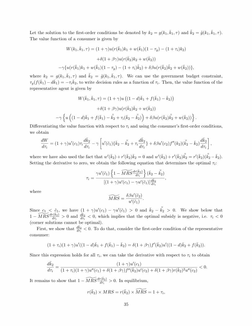
Let the solution to the first-order conditions be denoted by k2 = g(k1, k1, τ) and k2 = g(k1, k1, τ).The value function of a consumer is given by

W (k1, k1, τ) = (1 + γ)u(r(k1)k1 + w(k1)(1− τy)− (1 + τi)k2)

+δ(1 + βγ)u(r(k2)k2 + w(k2))

−γ{u(r(k1)k1 + w(k1)(1− τy)− (1 + τi)k2) + δβu(r(k2)k2 + w(k2))},

where k2 = g(k1, k1, τ) and k2 = g(k1, k1, τ). We can use the government budget constraint,τy(f(k1)− dk1) = −τik2, to write decision rules as a function of τi. Then, the value function of therepresentative agent is given by

W (k1, k1, τ) = (1 + γ)u((1− d)k1 + f(k1)− k2)

)+δ(1 + βγ)u(r(k2)k2 + w(k2))

−γ{

u((1− d)k1 + f(k1)− ¯

k2 + τi(k2 − ¯k2))

+ δβu(r(k2)¯k2 + w(k2))

}.

Differentiating the value function with respect to τi and using the consumer’s first-order conditions,we obtain

dW

dτi= (1 + γ)u′(c1)τi

dk2

dτi− γ

[u′(c1){k2 − ¯

k2 + τidk2

dτi}+ δβu′(c2)f ′′(k2)(

¯k2 − k2)

dk2

dτi

],

where we have also used the fact that w′(k2)+ r′(k2)k2 = 0 and w′(k2)+ r′(k2)¯k2 = r′(k2)(

¯k2− k2).

Setting the derivative to zero, we obtain the following equation that determines the optimal τi:

τi =γu′(c1)

{1− MRS dr(k2)

dτi

}(k2 − ¯

k2)

[(1 + γ)u′(c1)− γu′(c1)]dk2dτi

,

where

MRS =δβu′(c2)u′(c1)

.

Since c1 < c1, we have (1 + γ)u′(c1) − γu′(c1) > 0 and k2 − ¯k2 > 0. We show below that

1 − MRS dr(k2)dτi

> 0 and dk2dτi

< 0, which implies that the optimal subsidy is negative, i.e. τi < 0(corner solutions cannot be optimal).

First, we show that dk2dτi

< 0. To do that, consider the first-order condition of the representativeconsumer:

(1 + τi)(1 + γ)u′((1− d)k1 + f(k1)− k2) = δ(1 + βγ)f ′(k2)u′((1− d)k2 + f(k2)).

Since this expression holds for all τi, we can take the derivative with respect to τi to obtain

dk2

dτi=

(1 + γ)u′(c1)(1 + τi)(1 + γ)u′′(c1) + δ(1 + βγ)f ′′(k2)u′(c2) + δ(1 + βγ)r(k2)2u′′(c2)

< 0.

It remains to show that 1− MRS dr(k2)dτi

> 0. In equilibrium,

r(k2)×MRS = r(k2)× MRS = 1 + τi,

35

where

MRS =δ(1 + βγ)u′(c2)(1 + γ)u′(c1)

.

Therefore, it is enough to show that

1−MRSdr(k2)

dτi> 0.

Taking the derivative ofr(k2)×MRS = 1 + τi

with respect to τi, we obtain

dMRS

dτir(k2) + MRS

dr(k2)dτi

= 1.

Now r(k2) > 0 implies that 1−MRS dr(k2)dτi

> 0 if dMRSdτi

> 0. Given that

MRS =δ(1 + βγ)u′((1− d)k2 + f(k2))

(1 + γ)u′((1− d)k1 + f(k1)− k2)

and dk2dτi

< 0, it is then clear that dMRSdτi

> 0. Q.E.D.

Proof of Proposition 8: Let Y be present value lifetime income. We can show that in a twoperiod model with log utility, c1 = #1Y , c2 = #2

r(k2)1+τi

Y , c1 = #1Y , and c2 = #2r(k2)1+τi

Y . Constantsare just functions of preference parameters. Then lifetime utility of an agent is

W (k1, k1, τ) = a constant + u(c1) + δu(c2).

Following the same notation as in the proof of proposition 7, the lifetime utility of the repre-sentative consumer is

W (k1, k1, τ) = u((1− d)k1 + f(k1)− k2

)+ δu

(r(k2)k2 + w(k2)

)Taking derivative with respect to τ we get

dW

dτi=(−u′(c1) + δr(k2)u′(c2)

) dk2

dτi= 0.

Remember that dk2dτi

< 0, then the optimal government policy would imply that

u′(c1) = δr(k2)u′(c2).

Using the FOC of an individual which is

(1 + τi)(1 + γ)u′(c1) = δ(1 + βγ)r(k2)u′(c2).

the optimal subsidy is given by1 + βγ

(1 + γ)(1 + τi)= 1.

Q.E.D.

36

Appendix 2

This appendix describes how we use the four functional equations (6)–(9) to find a linear approx-imation to dynamic equilibrium behavior near a steady state. Local (linear) dynamics around asteady state can be determined by differentiating the four functional equations with respect to k,imposing the steady-state condition k′ = k = kss, and then solving for λ′(kss), µ′(kss), λ′(kss), andµ′(kss). The steady state is thus locally stable if λ′(kss)kss + λ(kss) + µ′(kss) is less than one inabsolute value.

In particular, we have implemented the following numerical algorithm for examining local dy-namics numerically. First, postulate that

λ(k) = 1 + λ′(kss)(k − kss)

µ(k) = µ′(kss)(k − kss)

λ(k) = λ(kss) + λ′(kss)(k − kss)

µ(k) = µ(kss) + µ′(kss)(k − kss),

where λ(kss), µ(kss), and kss are determined as described in the section on steady states and thefour first derivatives λ′(kss), µ′(kss), λ′(kss), and µ′(kss) are unknown parameters to be determinedby the numerical algorithm. Second, rewrite each of the equations (6)–(9) so that the right-handside is zero. Third, given values of the four first derivatives, use a finite-difference method toapproximate the derivatives with respect to k of the left-hand sides of each of the equations (6)–(9). Fourth, vary the four first derivatives in order to set the derivatives of the left-hand sides eachof the four equations equal to zero.

We could also use the four functional equations to study global (nonlinear) dynamics. Forexample, in the spirit of a weighted residual method, one could postulate that each of the fourfunctions is a polynomial in k with unknown coefficients and then choose the coefficients so thatEuler equation errors (i.e., errors in satisfying the four functional equations) are set to 0 at variouspoints in the state space. As described in Section 4.4.2 and in Appendix 3, we choose instead tostudy global dynamics (which we need to study for our policy experiments) by working directly withthe value function. The main advantage of doing so is that we need to solve only two, rather thanfour, functional equations. Given an approximation to the value function, we can then computeapproximations to both the actual and temptation decision rules.

Appendix 3

In this appendix we describe how we compute approximate (nonlinear) solutions to the two func-tional equations (11) and (12) that determine the consumer’s value function. We let a(k) be anth-order polynomial in log(k) with coefficients {ai}n

i=0 and we let b(k) be an nth-order polynomialin k with coefficients {bi}n

i=0.26

To find the coefficients of the two polynomials, we proceed as follows. First, given a guess forthe bi’s, use the consumer’s decision rule (13) to determine k′ as a function of k. That is, impose

26For a special case of this model in which the depreciation rate d equals 1 and τk = τl = τy, it turns out that a(k)is an affine function of log(k) and b(k) is proportional to k. For this reason, we choose to let a be a polynomial inlog k and b be a polynomial in k.

37

the equilibrium conditions k = k and k′ = k′ in this equation and then find (an approximationto) the function mapping k into k′. In practice, we choose a grid of values for k and then solvenumerically for k′ for each value of k on the grid. We then use cubic splines to interpolate betweenvalues on the grid. Second, use the function determined in the first step to express k′ as a functionof k in the functional equations (11) and (12). These equations now depend only on k. Third,pick n + 1 values of k and then choose the ai’s and bi’s so that both of these equations are exactlysatisfied at these n + 1 values. We use the simplex algorithm followed by Newton’s method withtwo-sided numerical derivatives to solve this set of 2(n+1) nonlinear equations in the ai’s and bi’s.

For the quantitative results reported below, we use 100 grid points for k in the first step. Thesegrid points are equally spaced in an interval containing two steady states, one for the case of notaxation and one for the case of a nonzero value for the subsidy τi. In the second step, where weset n = 4, the n + 1 values of k are equally spaced in an interval analogous to the one used in thefirst step.

38