How is it made?

Google Search Engine

Joseph Khoury

November 15, 2010

Abstract

If you are one of the millions of people around the planet who use a search engine on a daily basis,

you must have wondered at one point: how does the engine classify and display the information you are

looking for? What makes your "favorite" search engine different from other search engines in terms of

the relevance of the information you are looking for?

With billions of search requests a day, it is no surprise that Google is the search engine of choice of

web surfers around the globe. The Mathematics behind the Google search algorithm (PageRank) could,

however, come as a complete surprise to you. The purpose of this note is to explain, in as much self

contained content as possible, the mathematical reasoning behind the PageRank algorithm.

1 Introduction

The details of how exactly Google and other search engines look for information on the web and classify

the importance of the pages containing the information you are looking for are certainly kept secret within

a small circle of researchers and developers working for the company. However, at least for Google, the

main component of its search mechanism has been known for a while as the PageRank Algortithm. The

algorithm is named after Larry Page who, together with Sergey Brin, founded the company Google Inc in

the late 90’s. Here is how Google describes the PageRank algorithm on its cooperative site:

PageRank reflects our view of the importance of web pages by considering more than 500 million vari-

ables and 2 billion terms. Pages that we believe are important pages receive a higher PageRank and are

more likely to appear at the top of the search results. PageRank also considers the importance of each page

that casts a vote, as votes from some pages are considered to have greater value, thus giving the linked page

greater value. We have always taken a pragmatic approach to help improve search quality and create use-

ful products, and our technology uses the collective intelligence of the web to determine a page’s importance.

1

The main tool used by PageRank is the theory of Markov chains, a well known process developed by

the russian mathematician Andrei Markov at the beginning of the last century. In a nutshell, the process

consists of a countable number of states and some given probabilities pi j , with pi j being the probability

of moving from state j to state i .

Since algebra is the topic of the day, I decided to search the word "algebra" on both Google and Yahoo

search Engines.

What Yahoo considers to be the top page for providing information about the search topic (Algebra Home-

work Help) ranked fifth in Google’s ranking and the top page in Google’s ranking (Wikipedia) came second

in Yahoo’s listing. Not very surprising considering how well known the word "Algebra" is. But what is more

surprising is perhaps the fact that the page ranked fourth on Yahoo’s list does not appear as one of the top

100 on Google’s list. So who is to say what page contains more relevant information about "Algebra"? Is

it only a matter of trust between the user and his or her favorite Search Engine? Google is so confident of

its page ranking that it even added the "I am feeling lucky" button beside the search button that will take

you right to the page ranked 1 on its listing.

It turns out that, at least from Google’s perspective, a webpage is as important as the number of pages

in the hyper world that point or link to it. But that is just one part of the story.

2

To start, let us represent every webpage with a node (or a vertex). If there is link from page "A" to page

"B", then we make an arrow from node A to node B that we call an edge. The structure obtained is called

a (directed) graph. To simplify our discussion, let us look at a hyperworld containing only six pages with

the following links:

Example 1.1.

F

A

B

C

D

E

Note that a "double arrow" between two nodes means that there is a link from each of the two pages

to the other. For example, there a link from page C to page E and vice versa in the above network.

The PageRank algorithm is based on the behavior of a random web surfer that we will refer to as Joe for

simplicity. To surf the web, Joe would start at a page of his choice, then he randomly chooses a link from

that page to another page and would continue this process until arriving at a page with no exterior links

to other pages or until he (suddenly) decides to move to another page by other means than following a

link from a current page, like for instance entering the URL of a page in the address bar. Two important

aspects govern the behavior of Joe while surfing the web:

1. The choice of what page to visit next depends only on what page is Joe on now and not on the pages

he previously visited;

2. Joe is resilient, in the sense that he will never give up on moving from one page to another either by

following the link structure of the web or by other means.

Assume that there are n webpages in total (n ≈ 110000000 in 2009), the PageRank algorithm creates a

square n ×n matrix H , that we call the hyper matrix, as follows:

• We assume that the webpages are given a certain numerical order 1,2,3, . . . ,n, not necessarily by the

order of importance. We just "label" the webpages using the integers 1,2,3, . . . ,n.

3

• For any i , j ∈ {1,2, . . . ,n}, the entry hi j on the i th row and j th column of H represents the probability

that Joe would go from page j to page i in one move (or one click). In other words, if the webpage j

has a total of k j links to others pages then

hi j =

1k j

if there is a link from page j to page i

0 if there is no link from page j to page i

For the above model of Example 1.1, if the pages are ordered as follows A = 1, B = 2, C = 3, D = 4, E = 5

and F = 6, the hyper matrix is

H =

0 0 0 12

12 0

14 0 0 0 0 014 0 0 0 1

2 014

13

12 0 0 1

0 13

12

12 0 0

14

13 0 0 0 0

.

If we assume that there is an average of 10 links per page on the web, then the web hyper matrix is

extremely "sparse". That is, there is an average of only 10 nonzero entries in each column of the matrix

and the rest (billions of entries) are all zeros.

A page that does not link to any other page in the Network is called a dangling node. The presence

of a dangling node in a network creates a column of zeros in the corresponding hyper matrix since if Joe

lands on a dangling page, the probability that he leaves the page via a link is zero. Note that the Network

in Example (1.1) above has no dangling nodes, we will deal with the dangling nodes problem a bit later in

the discussion.

At any stage of the process, the notation pi (X ) represents the probability that Joe lands on page X

after i steps (or i clicks). If the page X is labeled using the integer j , then pi (X ) is denoted by pi j . The

vector pi :=[

pi 1 pi 2 . . . pi n

]t(where At means the transpose of the matrix A) is called the i th

probability distribution vector. We also define the initial probability vector as being the vector with all

0’s except for one entry equal to 1. That entry corresponds to the page were Joe initially starts his search.

In Example (1.1), if Joe starts his search at the page C , then the initial probability distribution vector is[0 0 1 0 0 0

]t.

Note that the i th column of the hypermatrix H is nothing but the initial probability vector correspond-

ing to a start at the page labeled i .

At this point, the following questions become relevant:

4

1. Can we determine the probability distribution vector after k steps (or k clicks)? In other words, can

we determine the probability of Joe being on page i of the web after k clicks?

2. Can we "predict" the behavior of Joe in the long run? That is, can we after a very big number of

clicks determine the probability of Joe being on page i for any i ∈ {1,2, . . . ,n}?

3. If such a long term behavior of Joe can be determined, does it depend on the initial probability

vector? That is, does it matter which page Joe starts his surfing with?

After certain refinements of the hypermatrix H , one can give definitive answers to all these questions.

Let us first look at some of these questions from the perspective of the 6-pages Network of Example

1.1. Assuming Joe starts at the page A, the initial distribution vector is p0 =[

1 0 0 0 0 0]t

.

After the first click, there is an equal probability of 14 that Joe lands on either one of the pages B ,C ,D or

F since these are the pages A links to. On the other hand, there is a zero probability that he lands on

page E (again by using links). This means that after the first click, the probability distribution vector is

p1 =[

0 14

14

14 0 1

4

]t. But note that

H p0 =

0 0 0 12

12 0

14 0 0 0 0 014 0 0 0 1

2 014

13

12 0 0 1

0 13

12

12 0 0

14

13 0 0 0 0

1

0

0

0

0

0

=

0141414

014

= p1

Similarly, if Joe’s initial distribution vector is p0 =[

0 0 0 1 0 0]t

(Joe starts at the page D), then

after the first click there is an equal probability of 12 to land on either one of the two pages A or E since

these are the pages D links to and zero probability that he lands on any of the pages B ,C ,D and F by

means of links. This suggests that after the first click, the probability distribution vector of Joe is p1 =[12 0 0 0 1

2 0]t

, and again

H p0 =

0 0 0 12

12 0

14 0 0 0 0 014 0 0 0 1

2 014

13

12 0 0 1

0 13

12

12 0 0

14

13 0 0 0 0

0

0

0

1

0

0

=

12

0

0

012

0

= p1.

This is hardly a coincidence. Suppose that the (only) entry 1 of the initial probability distribution vector

is at the i th component (Joe starts at page i ), then it is easy to see that H p0 is nothing but the i th column

5

of H which in turn is the probability distribution vector after the first click.

If pk is the probability distribution vector after the kth click (k ≥ 1), should we expect that pk = H pk−1?

Let us see what happens after the second click. Assume that Joe starts at the page A, then after the first

click he is at one of the pages B ,C ,D or F with equal probability 14 . What is the probability of Joe landing

on each of the pages after the second click? The answer depends on the paths available for Joe in his surf.

• The only way Joe can return to page A after the second click is that he follows the path A → D → A.

This path happens with a probability of 14 . 1

2 since once Joe is on page D he has two choices, page A

or page E. So, p2(A) = 18 after the second click.

• Note that the only way to land on page B is from page A, meaning that there is no chance on landing

on page B after the second click, p2(B) = 0.

• Since the only pages linking to C are A and E and since there is no link from A to E , the chance of

landing on C after the second click is zero, p2(C ) = 0.

• Landing on page D after the second click can de done through one of the following paths: A →C →D with probability 1

4 . 12 = 1

8 or A → C → D with probability 14 . 1

2 = 18 or A → F → D with probability

14 .1 = 1

4 . So, p2(D) = 18 + 1

12 + 14 = 11

24 .

• For the page E , Joe can reach it after the second click by following one of the following paths: A →B → E with probability 1

4 . 13 = 1

12 , A →C → E with probability 14 . 1

2 = 18 or A → D → E with probability

14 . 1

2 = 18 . So, p2(E) = 1

12 + 18 + 1

8 = 13 .

• For page F , the only possible path is A → B → F with probability p2(F ) = 14 . 1

3 = 112

Note that the network has no dangling pages, so Joe must land on one of the pages after the second click.

We should then expect that p2(A)+p2(B)+p2(C )+p2(D)+p2(E)+p2(F ) = 1:

1

8+0+0+ 11

24+ 1

3+ 1

12= 1.

The probability distribution vector after the second click is then p2 =[

18 0 0 11

2413

112

]t. One

must interpret the components of this vector as follows: starting at the page A and after the second click,

Joe will land on page A with a probability of 18 , on page D with a probability of 11

24 , on page E with a prob-

ability of 13 , on page F with a probability of 1

12 and there is no chance on landing on either one of pages B

and C after the second click.

A closer look at the components of this new distribution vector p2 reveals that they are obtained the

following way:

p2(A) = 1

8= 0.0+0.

1

4+0.

1

4+ 1

2.1

4+ 1

2.0+0.

1

4

6

which is exactly the product of the first row of the hypermatrix H with the previous distribution column

p1. Similarly, p2(B) is the same as the product of the second row of H with p1. Similar conclusions can be

drawn for the other probability values. In other words,

p2 = H p1 = H 2p0. (1.0.1)

Continuing to the third click and beyond, one can now see that equation (1.0.1) can be generalized to

pk+1 = H pk = H k p0 (1.0.2)

for any k ≥ 0. The first 20 probability distribution vectors for example (1.1) above are given below (with

components in decimal forms).

p0 =

1

0

0

0

0

0

, p1 =

0.5

0

0

0

0.5

0

, p2 =

0.125

0

0

0.4583

0.3333

0.0833

, · · · , p18 =

0.2319

0.0579

0.1670

0.2392

0.2239

0.0772

, p19 =

0.2315

0.0580

0.1699

0.2394

0.2239

0.0773

, p20 =

0.2317

0.0579

0.1698

0.2394

0.2240

0.0772

There is a clear indication that in the long run, Joe’s probability distribution vector will be close to the

vector

π=

0.231

0.058

0.169

0.239

0.224

0.078

In practical terms, this means that eventually Joe would visit page A with a probability of 23.1%, page B

with a probability of 5.8% and so on. The page with the highest chance to be visited is clearly D with a

probability of almost 24%. Note that the sum of the components of π is 1, making it a probability distri-

bution vector. One can then "rank" the pages in Example (1.1) according to their chances of being visited

after a sufficiently large walk of Joe on the Network: D, A, E, C, F, B would then be the order in which these

pages would appear. The ranking vector π is called the stationary distribution vector.

1.1 The dangling page problem

Example (1.1) seems to suggest that one can always rank the pages in any network just by making a suffi-

ciently large walk to estimate the long term behavior of the probability distribution vector. Nothing could

be further from the truth; things can get quickly out of hand if we consider a Network with dangling nodes

7

or a network with a trapping loop.

Let us slightly change the network in Example (1.1):

Example 1.2.

F

A

B

C

D

E

making F a dangling node. The hypermatrix of this new Network would be:

H =

0 0 0 12

12 0

14 0 0 0 0 014 0 0 0 1

2 014

13

12 0 0 0

0 13

12

12 0 0

14

13 0 0 0 0

Note that the last column is, as expected, the zero column due to the fact that page F does not link to

any other page in the network. Starting at the page A and proceeding exactly the same way as in Example

(1.1), the first 40 probability distribution vectors for Example (1.2) are (in decimal form):

p0 =

1

0

0

0

0

0

, p1 =

0

0.25

0.25

0.25

0

0.25

, p2 =

0.125

0

0

0.2083

0.3333

0.0833

, · · · , p38 =

0.0065

0.0018

0.0054

0.0054

0.0065

0.0024

, p39 =

0.0060

0.0016

0.0050

0.0050

0.0060

0.0022

, p40 =

0.0054

0.0015

0.0045

0.0045

0.0054

0.0020

which seems to suggest that in the long run, H pk is approaching the zero vector. The above "ranking"

procedure would not make much sense in this case.

8

1.2 The trapping loop problem

Another problem Joe could face following the link structure of the web is the chance that he could be

trapped in a loop. Let us once more modify the Network of Example (1.1):

Example 1.3.

F

A

B

C

D

E

In this new Network, if Joe happens to land on page B then the only path he could take is the loop

B → F → B → F → B → . . .

This suggests that the long term behavior of Joe can be described by the probability distribution vector

[ 0 12 0 0 0 1

2 ]t . In terms of page ranking, this means that pages B and F will "absorb" the im-

portance of all other pages in the network and that, of course, is not a reasonable ranking.

1.3 A possible Fix

In the light of the two complications Joe could face (dangling pages and trapping loops), one can refor-

mulate the above three questions we posed earlier using a more mathematical language.

Given a square n ×n matrix A and a vector p0 ∈Rn :

1. Does the sequence of vectors p0, p1 = Ap0, p2 = Ap1, . . . (and in general p j+1 = Ap j ) always "con-

verge" to a vector π?

2. If a vector π exists,

(a) Is it unique?

(b) Does it depend on the initial vector p0?

9

For networks like the one in Example (1.1), with no dangling pages or trapping loops, it seems that the

answers to allof these questions is yes. The sequence of Joe’s probability distribution vectors

p0, p1, p2, . . . , pk , . . .

converges to a probability vector π (the long term probability distribution vector) that could be inter-

preted as a "ranking" of the pages (nodes) in the Network. If the i th component of π is the largest, then

page i is ranked first, and so on.

In reality, a considerable percentage of actual webpages on the World Wide Web are indeed dangling

pages, either because they are simply pictures, pdf files, postscript files, Excel or words files and similar

forms or because at the time of the search Google data base was not updated. This makes the www hy-

perlink matrix a really sparse matrix, i.e a matrix with mostly zero entries. The above described algorithm

of surfing the web based on outgoing links seems to be unreal unless the above problems are addressed.

After landing on a dangling page, the probability that Joe leaves the page to another via a link is zero,

but he can still continue searching the web by other means, like for instance entering the Uniform Re-

source Locator (URL) directly into the web browser address bar. The following are two possible solutions

for the dangling pages problem.

• One can assume that Joe leaves a dangling page with an equal probability of 1n to visit any other

page (by means other than following links). Consider the dangling vector d which is the row vector

with the component di equals to 1 if page i is dangling and 0 otherwise. For example, the dangling

vector in Example 1.2 above is [ 0 0 0 0 0 1 ]t .

Form the "new hypermatrix"

S = H + 1

n1.d ,

where, as before, 1 is the column vector ofRn of all 1s. Simply put, the matrix S is obtained from H by

replacing every zero column in the original hypermatrix H with the column[

1n

1n · · · 1

n

]t.

The new matrix S is now stochastic (every column adds up to 1).

10

In Example (1.2), the new hypermatrix matrix is

S =

0 0 0 12

12 0

14 0 0 0 0 014 0 0 0 1

2 014

13

12 0 0 0

0 13

12

12 0 0

14

13 0 0 0 0

+ 1

6

1

1

1

1

1

1

[

0 0 0 0 0 1]

=

0 0 0 12

12 0

14 0 0 0 0 014 0 0 0 1

2 014

13

12 0 0 0

0 13

12

12 0 0

14

13 0 0 0 0

+

0 0 0 0 0 16

0 0 0 0 0 16

0 0 0 0 0 16

0 0 0 0 0 16

0 0 0 0 0 16

0 0 0 0 0 16

=

0 0 0 12

12

16

14 0 0 0 0 1

614 0 0 0 1

216

14

13

12 0 0 1

6

0 13

12

12 0 1

614

13 0 0 0 1

6

• Another way to deal with dangling pages is to start by removing them, together with all the links

leading to them, from the web. This will create a new well behaved (stochastic) hypermatrix that

will hopefully have a stationary distribution vector π. We then use π as a ranking vector for the

pages of the "new web". After this initial ranking is done, a dangling page X "inherits" the ranking

from pages linking to it as follows. If page k is one of the pages linking to X with a total of mk links

to X and if rk is the rank of page k, then we assign the sum

∑k

rk

mk

as the rank of the dangling page X (where k in the above sum runs over all the pages linking to X ). In

this fashion, the rankings of pages linking to a dangling page are in a way transferred to the dangling

page.

Although the new matrix S is stochastic, there is still no guarantee that it will have a stationary prob-

ability distribution vector that could be used as a ranking vector (see Definition (1.1) and Theorem (2.1)).

The inventors of PageRank (Page and Brin) made another adjustment to this end. While it is generally the

case that web surfers follow the link structure of the web, an actual surfer might decide from time to time

to "teleport" to a new page by entering a new destination in the address bar. From the new destination,

the surfer continues to follow the links until he decides once more to teleport to a new page. To capture

the surfer’s mood, Page and Brin introduced a new matrix, called the Google matrix, as follows.

G =αS + (1−α)1

n1.1t

where 1n 1.1

t is, of course, the n×n matrix where each entry is equal to 1n representing the uniformly prob-

able web teleporting process. α is a number between 0 and 1 called the "damping factor" representing

11

the proportion of times Joe teleports to a web page versus following the link the structure. For example, if

α= 0.8, then this would mean that 80% of the time Joe is following the link structure and 20% he teleports

to a randomly chosen page. Note that if α = 0, then G = 1n 1.1

t which means that Joe is teleporting all the

time he is on the web. On the other extreme, if α= 1, then G = S which means that Joe is always following

the link structure of the web. Realistically, α should then be strictly between 0 and 1 and more close to 1

than it is to 0 since Joe will more likely follow the links on the web. In the original article describing the

PageRank algorithm ([1]), the authors used a damping factor of α= 0.85.

Example 1.4. With α= 0.85, the Google matrix for the Network in Example (1.1) (with entries rounded to

4 decimal places) is given by

G =

0.2500 0.2500 0.2500 0.4500 0.4500 0.1667

0.2375 0.2500 0.2500 0.2500 0.2500 0.1667

0.2375 0.2500 0.2500 0.2500 0.4500 0.1667

0.2375 0.3083 0.4500 0.2500 0.2500 0.1667

0.2500 0.3083 0.4500 0.4500 0.2500 0.1667

0.2375 0.3083 0.2500 0.2500 0.2500 0.1667

.

For a general web, the Google matrix G satisfies the following properties:

• G is stochastic. In fact, write S = [si j ], then the sum of entries on the j th column of G is given by

n∑i=1

(αsi j + (1−α)

1

n

)=α

n∑i=1

si j︸ ︷︷ ︸=1

+n(1−α)1

n=α+ (1−α) = 1.

If j is a dangling page, then S j = 1n [1, 1 . . . ,1]t and the sum of the entries of the j th column of G

is in this case equal to α 1n [1, 1 . . . ,1]t + (1−α) 1

n [1, 1 . . . ,1]t = 1. If j is not a dangling page, then

S j = [h1 j , h2 j . . . ,hn j ]t (with∑n

i=1 hi j = 1) and the sum of the entries on the j th column of G is in

this case equal to

αn∑

i=1hi j + (1−α)

1

n

n∑i=1

1 =

α+ (1−α)1

nn = 1.

• G is positive. In fact, by the observation made above, the damping factor satisfies 0 < α < 1 (strict

inequalities). Write G = [gi j ], then gi j =αsi j + (1−α) 1n where si j is either 0 or 1

ki jfor some positive

integer ki j ≤ n. If si j = 0, then gi j = (1−α) 1n > 0. If si j = 1

ki jfor some positive integer ki j ≤ n, then

gi j =αsi j + (1−α)1

n=α

1

ki j+ (1−α)

1

n≥α

1

n+ (1−α)

1

n= 1

n> 0.

All entries of G are then positive.

12

In view of Theorem 2.1 below, the Google matrix G satisfies the desired requirements and will have a

stationary probability distribution vector. We are now ready to define the Google page ranking.

Definition 1.1. Let π = [ π1 π2 . . . πn ]t be the stationary probability distribution vector of the

Google matrix G . The Google rank of page i is defined to be i th component πi of the vector π. Page i

comes before page j in Google ranking if and only if πi >π j .

From a search engine marketer’s point of view, this means there are two ways in which PageRank can

affect the position of your page on Google.

2 The Mathematics of PageRank

We begin this section with a quick review of some basic notions necessary for a full understanding of the

mathematics behind Google’s search algorithm. Linear Algebra is the main tool used in this algorithm

and topics from this discipline are the main focus of review. The reader is assumed to be familiar with ba-

sic Matrix Algebra operations, like matrix addition, multiplication, inverse, determinant and algorithms

of solving linear systems. Also assumed are the notions of subspaces and bases and dimensions of sub-

spaces of Rn .

Throughout, A denotes an n ×n square matrix. The transpose of A is denoted by At .

2.1 The "Eigenstuff"

Definition 2.1. A nonzero vector X of Rn is called an eigenvector of A if there exists a scalar λ such that

AX =λX . (2.1.1)

The scalar λ is called an eigenvalue of A corresponding to the eigenvector X .

Note that relation (2.1.1) can be written as (A −λI )X = 0, where I is the n ×n identity matrix (having

1 on the main diagonal and 0 everywhere else). This shows that X is a solution to the linear homoge-

neous system (A −λI )X = 0. The fact that X is assumed to be a nonzero vector implies that the system

(A −λI )X = 0 has a nontrivial solution and consequently, the coefficient matrix (A −λI ) is not invert-

ible. Therefore, det(A −λI ) = 0 where "det" stands for the determinant of the matrix. The expression

det(A −λI ) is clearly a polynomial of degree n in the variable λ usually referred to as the characteristic

polynomial of A.

This suggests the following steps to find the eigenvalues and eigenvectors of A:

1. To find the eigenvalues of A, one has to find the roots of the characteristic polynomial of A; i.e, to

solve the equation det(A −λI ) = 0, called the characteristic equation of A, for the variable λ. This

13

is a polynomial equation of degree n in the variable λ which has n roots (not necessary distinct and

could be complex numbers)

2. The set Eλ of all eigenvectors corresponding to an eigenvalue λ of A, together with the zero vector,

form a subspace of Rn called the eigenspace corresponding to the eigenvalue λ. One usually needs

a basis of Eλ. To this end, we solve the homogeneous system (A−λI )X = 0. As the coefficient matrix

(A −λI ) is not invertible, one should expect infinitely many solutions. Writing the general solution

of the system (A−λI )X = 0 gives a basis of Eλ.

Example 2.1. Find the eigenvalues of the given matrix, and for each eigenvalue find a basis for the corre-

sponding eigenspace.

A =

2 2 1

1 3 1

1 2 2

.

Solution.

Using the properties of the determinant, the characteristic polynomial of A is∣∣∣∣∣∣∣∣2−λ 2 1

1 3−λ 1

1 2 2−λ

∣∣∣∣∣∣∣∣=∣∣∣∣∣∣∣∣

2−λ 2 1

1 3−λ 1

0 λ−1 1−λ

∣∣∣∣∣∣∣∣= (λ−1)

∣∣∣∣∣∣∣∣2−λ 2 1

1 3−λ 1

0 1 −1

∣∣∣∣∣∣∣∣= (λ−1)

∣∣∣∣∣∣∣∣2−λ 2 3

1 3−λ 4−λ

0 1 0

∣∣∣∣∣∣∣∣=−(λ−1)

∣∣∣∣∣ 2−λ 3

1 4−λ

∣∣∣∣∣=−(λ−1)(λ2 −6λ+5) =−(λ−1)2(λ−5)

The eigenvalues of A are then λ1 = 1 of algebraic multiplicity 2 and λ1 = 5 of algebraic multiplicity 1.

For the eigenspace corresponding to λ1 = 1, we write the general solution of the homogeneous system

(A−λ1I )X = 0 (I being the 3×3 identity matrix):∣∣∣∣∣∣∣∣2−λ1 2 1 : 0

1 3−λ1 1 : 0

1 2 2−λ1 : 0

∣∣∣∣∣∣∣∣=∣∣∣∣∣∣∣∣

1 2 1 : 0

1 2 1 : 0

1 2 1 : 0

∣∣∣∣∣∣∣∣∼∣∣∣∣∣∣∣∣

1 2 1 : 0

0 0 0 : 0

0 0 0 : 0

∣∣∣∣∣∣∣∣The two variables x2 and x3 are free variables, and x1 =−2x2 −x3. So the general solution of the homoge-

neous system (A−λ1I )X = 0 is:x1

x2

x3

=

−2x2 −x3

x2

x3

= x2

−2

1

0

+x3

−1

0

1

= x2v1 +x3v2.

14

So Eλ1 = span{v1, v2}. Since v1 and v2 are linearly independent, they form a basis of the eigenspace Eλ1 .

For the eigenspace corresponding to λ2 = 5, we write the general solution of the homogeneous system

(A−λ2I )X = 0:∣∣∣∣∣∣∣∣2−λ2 2 1 : 0

1 3−λ2 1 : 0

1 2 2−λ2 : 0

∣∣∣∣∣∣∣∣=∣∣∣∣∣∣∣∣−3 2 1 : 0

1 −2 1 : 0

1 2 −3 : 0

∣∣∣∣∣∣∣∣∼∣∣∣∣∣∣∣∣

1 −2 1 : 0

−3 2 1 : 0

1 2 −3 : 0

∣∣∣∣∣∣∣∣∼∣∣∣∣∣∣∣∣

1 −2 1 : 0

0 −4 4 : 0

0 4 −4 : 0

∣∣∣∣∣∣∣∣∼

∣∣∣∣∣∣∣∣1 −2 1 : 0

0 1 1 : 0

0 0 0 : 0

∣∣∣∣∣∣∣∣∼∣∣∣∣∣∣∣∣

1 0 3 : 0

0 1 1 : 0

0 0 0 : 0

∣∣∣∣∣∣∣∣Only x3 is a free variable. Moreover, x1 = −3x3 and x2 = −x3. This shows that the eigenspace Eλ2 is one-

dimensional with the vector [ −3 −1 1 ]t as a basis.

Lemma 2.1. (1) The characteristic polynomials of A and At are equal. In particular, a square matrix has

the same eigenvalues as its transpose;

(2) If v is an eigenvector of A corresponding to the eigenvalue λ, then for any non-negative integer k, v is an

eigenvector of Ak corresponding to the eigenvalue λk .

Proof

(1) The proof relies on the fact that the determinant of a square matrix is equal to the determinant of its

transpose. If cA(λ) is the characteristic polynomial of A, then

cA(λ) = det (A−λI ) = det (A−λI )t = det (At −λI t ) = det (At −λI ) = cAt (λ).

The second statement follows directly from the definition of an eigenvalue.

(2) Let v be an eigenvector corresponding to λ. Then Av =λv . If k > 0, then

Ak v = Ak−1(Av) = Ak−1(λv) = Ak−2(λAv) = Ak−2(λ2v) = ·· · = A0(λk v) = I (λk v) =λk v.

This shows that λk is an eigenvalue of Ak corresponding to the eigenvector v .

2.2 Stochastic matrices

Google PageRank Algorithm uses a special "probabilistic approach" to rank the importance of pages on

the web. The probability of what page a virtual surfer chooses to visit next depends solely on the current

page the surfer is on and not on pages he previously visited. The matrices arising from such an approach

are called stochastic.

Definition 2.2. The square matrix A = [ai j ] is called stochastic if each of its entries is a non-negative real

number and the entries on each column add up to 1. In other words

∀i , j , ai j ≥ 0 and for each k,n∑

s=1ask = 1.

15

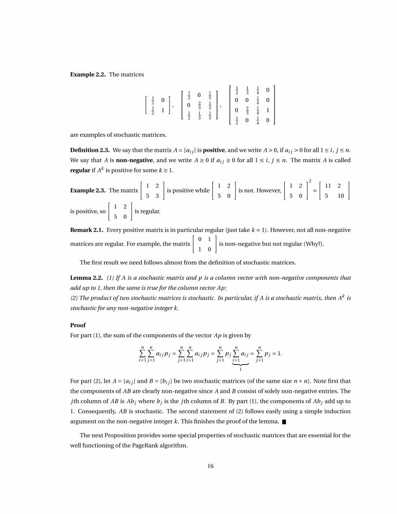
Example 2.2. The matrices

[12 012 1

],

12 0 1

3

0 23

13

12

13

13

,

12

13

14 0

0 0 14 0

0 23

14 1

12 0 1

4 0

are examples of stochastic matrices.

Definition 2.3. We say that the matrix A = [ai j ] is positive, and we write A > 0, if ai j > 0 for all 1 ≤ i , j ≤ n.

We say that A is non-negative, and we write A ≥ 0 if ai j ≥ 0 for all 1 ≤ i , j ≤ n. The matrix A is called

regular if Ak is positive for some k ≥ 1.

Example 2.3. The matrix

[1 2

5 3

]is positive while

[1 2

5 0

]is not. However,

[1 2

5 0

]2

=[

11 2

5 10

]

is positive, so

[1 2

5 0

]is regular.

Remark 2.1. Every positive matrix is in particular regular (just take k = 1). However, not all non-negative

matrices are regular. For example, the matrix

[0 1

1 0

]is non-negative but not regular (Why?).

The first result we need follows almost from the definition of stochastic matrices.

Lemma 2.2. (1) If A is a stochastic matrix and p is a column vector with non-negative components that

add up to 1, then the same is true for the column vector Ap;

(2) The product of two stochastic matrices is stochastic. In particular, if A is a stochastic matrix, then Ak is

stochastic for any non-negative integer k.

Proof

For part (1), the sum of the components of the vector Ap is given by

n∑i=1

n∑j=1

ai j p j =n∑

j=1

n∑i=1

ai j p j =n∑

j=1p j

n∑i=1

ai j︸ ︷︷ ︸1

=n∑

j=1p j = 1.

For part (2), let A = [ai j ] and B = [bi j ] be two stochastic matrices (of the same size n ×n). Note first that

the components of AB are clearly non-negative since A and B consist of solely non-negative entries. The

j th column of AB is Ab j where b j is the j th column of B . By part (1), the components of Ab j add up to

1. Consequently, AB is stochastic. The second statement of (2) follows easily using a simple induction

argument on the non-negative integer k. This finishes the proof of the lemma.

The next Proposition provides some special properties of stochastic matrices that are essential for the

well functioning of the PageRank algorithm.

16

Proposition 2.1. If A = [ai j ] is a stochastic matrix, then the following hold.

1. λ= 1 is an eigenvalue for A;

2. If A is regular, then any eigenvector corresponding to the eigenvalue 1 of A has all positive or all

negative components;

3. If λ is any eigenvalue of A, then |λ| ≤ 1;

4. If A is regular, then for any eigenvalue λ of A other than 1 we have |λ| < 1.

Proof

Consider the vector 1= [ 1 1 . . . 1 ] of Rn . The i th component of the vector At 1t is given by

n∑k=1

aki .1 =n∑

k=1aki = 1

since A is stochastic. This shows that At 1t = 1t and soλ= 1 is an eigenvalue of At with 1t as corresponding

eigenvector. Lemma 2.1 shows that λ= 1 is an eigenvalue for A. Part 1 of the Proposition is proved.

For part 2, we may assume that A is positive by the second part of Lemma 2.1. We use a proof by

contradiction. Let v = [ v1 v2 . . . vn ]t be an eigenvector of the eigenvalue 1 containing components

of mixed signs. Since Av = v , we have that vi = ∑nk=1 ai k vk and the terms ai k vk in this sum are of mixed

signs since ai k > 0 for each k. Therefore,

|vi | =∣∣∣∣∣ n∑k=1

ai k vk

∣∣∣∣∣< n∑k=1

ai k |vk | (2.2.1)

by the triangular inequality. The strict inequality occurs because the terms ai k vk in this sum are of mixed

signs. Taking the sum from i = 1 to i = n on both sides in (2.2.1) yields:

n∑i=1

|vi | <n∑

i=1

n∑k=1

ai k |vk | =n∑

k=1

(n∑

i=1ai k

)︸ ︷︷ ︸

=1

|vk | =n∑

k=1|vk |.

This is clearly a contradiction. We conclude that the vector v cannot have both positive and negative

components at the same time. Assume that vi ≥ 0 for all i , then for each i , the relation vi = ∑nk=1 ai k vk

together with the fact that ai k > 0 imply that vi > 0 since at least one of the vk ’s is not zero (v is an eigen-

vector). Similarly, if vi ≤ 0 for all i then vi < 0 for all i . This proves part 2 of the Proposition

For part (3), we use again the fact that A and At have the same eigenvalues. Let λ be any eigenvalue of

At and let v = [ v1 v2 . . . vn ]t ∈ Rn be a corresponding eigenvector. Suppose that the component

v j of v satisfies |v j | = max{|vi |; i = 1, . . .n} so that for any l = 1,2, . . . ,n, |vl | ≤ |v j |. By taking the absolute

values of the j th components on both sides of λv = At v , we get that |λv j | =∣∣∑n

i=1 ai j vi∣∣. Therefore,

|λv j | = |λ||v j | =∣∣∣∣∣ n∑i=1

ai j vi

∣∣∣∣∣ ≤n∑

i=1ai j |v j | = |v j |

n∑i=1

ai j = |v j |(

sincen∑

i=1ai j = 1

)

17

The inequality |λ||v j | ≤ |v j | implies that |λ| ≤ 1 (remember that |v j | 6= 0) and part (3) is proved.

For part 4, assume first that A (hence At ) is a positive matrix. Let λ be an eigenvalue of At with |λ| = 1.

We show that λ = 1. As in the proof of part 3, let v = [ v1 v2 . . . vn ]t ∈ Rn be a an eigenvector

corresponding to λ with |v j | = max{|vk |, k = 1, . . . ,n}, then

|v j | = 1.|v j | = |λ||v j | = |λv j | =∣∣∣∣∣ n∑i=1

ai j vi

∣∣∣∣∣≤ n∑i=1

ai j |vi | ≤n∑

i=1ai j︸ ︷︷ ︸

=1

|v j | = |v j |. (2.2.2)

This shows that the last two inequalities in (2.2.2) are indeed equal signs (bounded on the left and on the

right by |v j |). The first inequality is an equal sign if and only if all the terms in the sum∑n

i=1 ai j vi have

the same sign (all positive or all negative) and hence all the vi ’s are of the same sign (note that this gives

another proof of part 2). The fact that the second inequality is indeed an equal sign gives

n∑i=1

ai j (|v j |− |vi |) = 0. (2.2.3)

But ai j > 0 and |v j | − |vi | ≥ 0 for all i = 1,2, . . . ,n. Equation (2.2.3) implies that |v j | − |vi | = 0 for all

i = 1,2, . . . ,n. This, together with the fact that all the vi ’s have the same sign, imply that the vector v is

a scalar multiple of 1 = [ 1 1 . . . 1 ]t . This shows that the eigenspace of At corresponding to the

eigenvalue λ is one dimensional equals to span{1}. In particular, 1 is an eigenvector corresponding to λ

and consequently, At 1= λ1. But the vector 1 also satisfies At 1= 1 by the proof of part (1) of this Proposi-

tion. This shows that λ1= 1 which forces λ to equal 1.

Assume next that A is regular and choose a positive integer k such that Ak > 0. Let λ be an eigenvalue

of A satisfying |λ| = 1. Then part 2 of Lemma 2.1 shows that λk is an eigenvalue of Ak and λk+1 is an

eigenvalue of Ak+1. Since both Ak and Ak+1 are positive matrices, we must have that λk = λk+1 = 1 (by

the proof of the positive case). This last relation can be rearranged as λk (λ−1) = 0 which gives that λ= 1

since λk 6= 0 (remember we are assuming that |λ| = 1).

To prove the main Theorem behind PageRank algorithm, we still need a couple of basic results.

Lemma 2.3. Let n ≥ 2, u, v two linearly independent vectors in Rn . Then, we can choose two scalars s and

t not both zero at the same time such that the vector w = su + t v has components of mixed signs.

Proof

The fact that the vectors u, v are linearly independent implies that none of them is the zero vector. Let

α be the sum of all the components of the vector u. If α = 0, then u must contain components of mixed

signs. The values s = 1 and t = 0 will do the trick in this case. If α 6= 0, let s =−βα where β is the sum of all

the components of the vector v . For t = 1, the sum of the components of the vector w = su+t v is zero. On

the other hand, the vector w is nonzero since otherwise the vectors u and v would be linearly dependent.

We conclude that the components of w are of mixed signs.

18

Proposition 2.2. If A is a regular and stochastic matrix, then the eigenspace corresponding to the eigen-

value 1 of A is one-dimensional.

Proof

Suppose not. Then we can choose two linearly independent eigenvectors u, v corresponding to the eigen-

value 1. By Lemma (2.3) above, we can choose two scalars s and t not both zero at the same time such that

the vector w = su+ t v has components of mixed signs. The vector w is also an eigenvector corresponding

to the eigenvalue 1 of A. That is a contradiction to part 2 of proposition (2.1). This shows that no two

eigenvectors of the eigenvalue 1 can be linearly independent. Hence, the eigenspace corresponding to

the eigenvalue 1 is one-dimensional.

We now can state and prove the main Theorem of this section.

Theorem 2.1. If A is an n×n regular stochastic matrix, then there exists a unique vectorπ= [ π1 π2 . . . πn ]t ∈Rn such that Aπ=π and

n∑i=1

πi = 1, and πi > 0 for all i = 1, . . . ,n.

Proof

By Propositions 2.2 and 2.1 above, the eigenspace E1 corresponding to the eigenvalue 1 of A can be written

as E1 = Span{v} for some vector v with all positive or all negative components. Let π= 1a v where a is the

sum of all components of v . Then π is also an eigenvector of A corresponding to the eigenvalue 1 (hence

Aπ=π) and it is the only one satisfying the required conditions.

2.3 An eigenvector for a 25000000000×25000000000 matrix, really?

In theory, the Google matrix has a stationary probability distribution vector π, which is an eigenvector

corresponding to the eigenvalue 1 of the matrix. This should be, at least in theory, a straightforward task

that can be done by any student who completed a first year university linear algebra course. But remem-

ber that we are dealing with an n×n matrix with n measured in billions and maybe in trillions by the time

you read this work. Even the most powerful machines and computational algorithms we have in our days

will have enormous difficulties computing π.

One of the oldest and simplest methods to compute numerically the eigenvector of a given square ma-

trix is what is known in the literature as the power method. This method is simple, elementary and easy

to implement in a computer algebra software, provided that the matrix has a dominant eigenvalue (that

is an eigenvalue that is strictly larger in absolute value than any other eigenvalue of the matrix), but it is in

general slow in giving a satisfactory estimation. However, considering the nature of the Google matrix G ,

the power method is well-suited to compute the stationary probability distribution vector. This compu-

tation was described by Cleve Moler, the founder of Matlab as "The World’ s Largest Matrix Computation"

19

in an article published in Matlab newsletter in October 2002.

To explain the power method, we will assume for simplicity that the Google matrix G , in addition of

being positive and stochastic, has n distinct eigenvalues, although this is not a necessary condition. This

makes G a diagonalizable matrix and one can choose a basis {v1, v2, . . . , vn} ofRn formed by eigenvectors

of G (each vi is an eigenvector of G). By Proposition 2.1 above, we know that λ = 1 is a dominant eigen-

value (part 4 of Proposition 2.1). Rearrange the eigenvectors v1, v2, . . . , vn of G so that the corresponding

eigenvalues decrease in absolute value:

1 > |λ2| ≥ |λ3| ≥ . . . ≥ |λn |

with the first inequality being strict. Note also that for each i , and for each positive integer k, we have

Gk vi =Gk−1(Gvi ) =Gk−1(λi vi ) =λi Gk−1vi = . . . =λik vi . (2.3.1)

We can clearly assume that v1 =π is G’s stationary probability distribution vector. Starting with any vector

p0 ∈Rn with non-negative components that add to 1, we write p0 in terms of the basis vectors:

p0 = a1π+a2v2 +·· ·+an vn , (2.3.2)

where each ai is a real number. Then we compute the vectors

p1 =Gp0, p2 =Gp1 =G2p0, . . . , pk =Gpk−1 =Gk p0, . . .

Using the decomposition of p0 given in 2.3.2 and relation 2.3.1 above we can write

pk =Gk p0 = Gk [a1π+a2v2 +·· ·+an vn]

= a11kπ+λ2k v2 +·· ·+λn

k vn

= a1π+λ2k v2 +·· ·+λn

k vn .

By Lemma 2.2 above, the sum of the components of the vector Gk p0 is 1. Taking the sum of components

on each side of the equation Gk p0 = a1π+λ2k v2 +·· ·+λn

k vn gives

1 = a1

n∑j=1

π j +n∑

j=1

n∑i=2

a jλ jk v j i = a1 +

n∑j=1

n∑i=2

a jλ jk v j i . (2.3.3)

Since |λi | < 1 for each i = 2, . . . ,n, limk→+∞λik = 0 and so taking the limit as k approaches infinity on both

sides of equation (2.3.3) gives that a1 = 1. Therefore,

pk =Gk p0 =π+λ2k v2 +·· ·+λn

k vn . (2.3.4)

Again, taking the limit as k approaches infinity gives that the sequence of vectors p0, Gp0, G2p0, . . . , Gk p0, . . .

converges to the stationary probability distribution vector π.

20

In theory, one can use the power method to estimate π. But how many iterations do we need to com-

pute in order to get an acceptable approximation of π? In other words, what value of k should we choose

in order for Gk p0 to be "close enough" to π? The answer is in the magnitude of the second largest eigen-

value (in absolute value). To see this, denote by ‖v‖ the "norm" of v = [ v1 v2 . . . vn ] ∈ Rn in the

following sense:

‖v‖ =n∑

i=1|vi |.

Scaling the vectors vi ’s in the basis considered above by replacing each vi with 1‖vi ‖ vi (the vector π being

already of norm 1) gives a new "normalized" (each vector is of norm 1) basis formed also by eigenvectors

of G . We can then assume without loss of generality that ‖vi‖ = 1 for all i = 2,3, . . . ,n. Taking the norm on

both sides of 2.3.4 gives

‖pk −π‖ = ‖λ2k v2 +λ3

k v3 +·· ·+λnk vn‖ ≤ |λ2|k ‖v2‖+|λ3|k ‖v3‖+·· ·+ |λn |k ‖vn‖

= |λ2|k(‖v2‖+

∣∣∣∣λ3

λ2

∣∣∣∣k

‖v3‖+·· ·+∣∣∣∣λn

λ2

∣∣∣∣k

‖vn‖)

= |λ2|k(

1+∣∣∣∣λ3

λ2

∣∣∣∣k

+·· ·+∣∣∣∣λn

λ2

∣∣∣∣k)

As k approaches infinity, ‖pk −π‖ ≤ |λ2|k since∣∣∣ λiλ2

∣∣∣< 1 for each i = 3,4, . . . ,n. So, |λ2|k serves as an upper

bound on the error in estimating π using pk , and so the smaller |λ2| is, the better this approximation and

the quicker the convergence of the sequence is.

It was proven that for the Google matrix G = αS + (1−α) 1n 1.1

t , λ2 = α ([2]). This creates a bit of a

dilemma since on one hand, one wants to make α closer to 1 than 0 to reflect the fact that Joe follows

the link structure more often than teleporting on a new page, and on the other hand one would like to

consider smaller values for α to accelerate the convergence of the iteration sequence given by pk =Gk p0

and get the estimate for the ranking vector π. The compromise was to take α= 0.85. With this choice, Brin

and Page reported that between 50 and 100 iterations are required to obtain a decent approximation to π.

The calculation is reported to take a few days to complete.

Another particularity of the Google matrix G that makes the power method very practical in this case is

the fact that its hypermatrix component is very sparse. Recall that G =αS+ (1−α) 1n 1.1

t , and S = H + 1n 1.d

as above, so

Gpk =[α

(H + 1

n1.d

)+ (1−α)

1

n1.1t

].pk

= αH .pk +α

n1.d .pk +

(1−α)

n1.1t .pk

= αH .pk +α

n1.d .pk +

(1−α)

nB.pk

21

where B = 1.1t is the constant matrix where each entry is 1. Since most of the entries in H are zeros, com-

puting H .pk requires very little effort (on average, only ten entries per column of H are nonzero). The

computations αn 1.d .pk and (1−α)

n B.pk can be done by simply adding the current probabilities (compo-

nents of pk ) to the dangling pages and all the web pages respectively.

2.4 Summary

First one has to understand that Google PageRank is only one ranking criteria Google uses. You can think

of it as a multiplying factor in the global Google relevance algorithm. The higher this factor is, the more

important the page is.

Unlike what most people think, the PageRank algorithm has absolutely nothing to do with the rele-

vance of the search terms you enter in the Google bar. It is again only one aspect of the global Google

ranking algorithm. Links leading to a page X and links out from from pages linking to X have the bigger

effect.

Here are the basic steps in the period before and after you enter your query.

• Google is continuously crawling the web in real time with software called “Googlebots”. A Google

crawler visits a page, copies the content and follows the links from that page to the pages linked to

it, repeating this process over and over until it has crawled billions of pages on the web.

• After processing these pages and their contents, Google creates an index similar in its idea to a

normal index you find at the end of a book.

• However, Google index is different from a regular index since not only topics are displayed but rather

every single word a crawler has recorded together with their location on the pages and other infor-

mation.

• Because of the size of Google index, it is divided into pieces and stored on thousands of machines

around the globe.

• So every time you enter a query in Google search box, the query is sent to Google computers (de-

pending on your geographic location).

• Google algorithm first calculates the relevance of pages containing the search words in its index

creating a preliminary list.

• The "relevance" of each page on this preliminary list is then multiplied with the corresponding

PageRank of the page to produce the final list on your screen (together with a short text summary

for each result).

It is amazing what a little knowledge of Mathematics can produce.

22

References

[1] Lawrence Page, Sergey Brin, Rajeev Motwani, Terry Winograd, The PageRank citation ranking:

Bringing order to the Web, Stanford Technical report, 1999.

[2] Taher Haveliwala, Sepandar Kamvar, The second eigenvalue of the Google matrix, Stanford Techni-

cal report, June, 2003.

23