A&A 639, A139 (2020)https://doi.org/10.1051/0004-6361/202037739c© K. L. Yeo et al. 2020

Astronomy&Astrophysics

How faculae and network relate to sunspots, and the implicationsfor solar and stellar brightness variations

K. L. Yeo1, S. K. Solanki1,2, and N. A. Krivova1

1 Max-Planck Institut für Sonnensystemforschung, Justus-von-Liebig-Weg 3, 37077 Göttingen, Germanye-mail: yeo@mps.mpg.de

2 School of Space Research, Kyung Hee University, Yongin 446-701, Gyeonggi, Korea

Received 14 February 2020 / Accepted 15 June 2020

ABSTRACT

Context. How global faculae and network coverage relates to that of sunspots is relevant to the brightness variations of the Sun andSun-like stars.Aims. We aim to extend and improve on earlier studies that established that the facular-to-sunspot-area ratio diminishes with totalsunspot coverage.Methods. Chromospheric indices and the total magnetic flux enclosed in network and faculae, referred to here as “facular indices”,are modulated by the amount of facular and network present. We probed the relationship between various facular and sunspot indicesthrough an empirical model, taking into account how active regions evolve and the possible non-linear relationship between plageemission, facular magnetic flux, and sunspot area. This model was incorporated into a model of total solar irradiance (TSI) to elucidatethe implications for solar and stellar brightness variations.Results. The reconstruction of the facular indices from the sunspot indices with the model presented here replicates most of theobserved variability, and is better at doing so than earlier models. Contrary to recent studies, we found the relationship between thefacular and sunspot indices to be stable over the past four decades. The model indicates that, like the facular-to-sunspot-area ratio, theratio of the variation in chromospheric emission and total network and facular magnetic flux to sunspot area decreases with the latter.The TSI model indicates the ratio of the TSI excess from faculae and network to the deficit from sunspots also declines with sunspotarea, with the consequence being that TSI rises with sunspot area more slowly than if the two quantities were linearly proportionalto one another. This explains why even though solar cycle 23 is significantly weaker than cycle 22, TSI rose to comparable levelsover both cycles. The extrapolation of the TSI model to higher activity levels indicates that in the activity range where Sun-like starsare observed to switch from growing brighter with increasing activity to becoming dimmer instead, the activity-dependence of TSIexhibits a similar transition. This happens as sunspot darkening starts to rise more rapidly with activity than facular and networkbrightening. This bolsters the interpretation of this behaviour of Sun-like stars as the transition from a faculae-dominated to a spot-dominated regime.

Key words. Sun: activity – Sun: faculae, plages – Sun: magnetic fields – sunspots

1. Introduction

The variation in solar irradiance at timescales greater than a dayis believed to be dominantly driven by photospheric magnetism(Solanki et al. 2013; Yeo et al. 2017a). Models developed toreproduce solar irradiance variability by relating it to magneticactivity on the solar surface provide the radiative forcing inputrequired by climate simulations (Haigh 2007). Solar irradiancevariability is modelled as the sum effect of the intensity deficitfrom sunspots and the excess from faculae and network, deter-mined from observations of solar magnetism (Domingo et al.2009; Yeo et al. 2014a). Most of the models aimed at recon-structing solar irradiance variability back to pre-industrial times,a period of particular interest to climate studies, rely on sunspotindices such as the total sunspot area, international sunspot num-ber, and group sunspot number, as these are the only directobservations of solar magnetic features to go this far back intime (e.g. Lean 2000; Krivova et al. 2007, 2010; Dasi-Espuiget al. 2014, 2016; Coddington et al. 2016; Wu et al. 2018). Ofcourse, inferring the effect of not just sunspots but also of facu-lae and network on solar irradiance from sunspot indices requiresknowledge of how the amount of faculae and network present

relates to sunspots. For example, the solar irradiance reconstruc-tion by Dasi-Espuig et al. (2014, 2016) made use of the modelby Cameron et al. (2010), which incorporates the empirical rela-tionship between facular and sunspot area reported by Chapmanet al. (1997), to calculate the amount of faculae and networkpresent from the sunspot area and number.

The understanding of how faculae and network relate tosunspots is also relevant to that of the brightness variations ofSun-like stars. The synoptic programmes at the Fairborn, Low-ell, and Mount Wilson observatories monitored the brightnessand activity of a number of Sun-like stars as indicated by theStrömgren b and y (i.e. visible) photometry and Ca II H&Kemission (as a proxy of activity). These observations revealeda dichotomy in the relationship between brightness and activ-ity. While the brightness of less active, older stars rises withincreasing activity, it diminishes for more active, younger stars(Lockwood et al. 2007; Hall et al. 2009; Shapiro et al. 2014;Radick et al. 2018). This switch in activity-dependence is inter-preted as the transition from a faculae-dominated regime, wherethe intensity excess from faculae and network has a greatereffect on brightness variations than the deficit from starspots,to a spot-dominated regime where the converse is true. The

Open Access article, published by EDP Sciences, under the terms of the Creative Commons Attribution License (https://creativecommons.org/licenses/by/4.0),which permits unrestricted use, distribution, and reproduction in any medium, provided the original work is properly cited.

Open Access funding provided by Max Planck Society.

A139, page 1 of 13

A&A 639, A139 (2020)

threshold between the two regimes is estimated to be at log R′HK(see definition in Noyes et al. 1984) of between −4.9 and−4.7 (Lockwood et al. 2007; Hall et al. 2009; Shapiro et al.2014; Radick et al. 2018; Reinhold et al. 2019). The Sun hasa mean log R′HK of about −4.9 (see Lockwood et al. 2007, andSect. 4.3) and appears to be faculae-dominated (Shapiro et al.2016; Radick et al. 2018), suggesting that it lies not far belowthis threshold. The transition between the faculae-dominated andspot-dominated regimes can therefore be probed by looking athow solar faculae and network relate to sunspots and by extrap-olating the apparent relationship to higher activity levels.

Chapman et al. (1997) examined the relationship betweentotal sunspot area and Ca II K plage area, taken as a proxy of fac-ular area, over the declining phase of solar cycle 22. This makesuse of the fact that chromospheric emission is strongly enhancedin plage and network features overlaying photospheric faculaeand network (e.g. Schrijver et al. 1989; Harvey & White 1999;Loukitcheva et al. 2009; Kahil et al. 2017; Barczynski et al.2018). Chapman et al. (1997) found that facular area conforms toa quadratic relationship with sunspot area. The coefficient of thesecond-order term is negative, such that the facular-to-sunspot-area ratio decreases as sunspot area increases. Investigations byFoukal (1993, 1996, 1998) and Shapiro et al. (2014), extendingmultiple solar cycles, returned similar results. However, whileChapman et al. (1997) made use of modern, relatively pristineCa II K spectroheliograms, Foukal (1993, 1996, 1998) lookedat facular areas based on historical Ca II K spectroheliograms,which suffer from calibration issues and defects (Ermolli et al.2009), and white-light heliograms, where the intensity contrastof faculae is not only weak, but also diminishes towards the disccentre (Foukal et al. 2004). While Chapman et al. (1997) andFoukal (1993, 1996, 1998) made use of measured facular area,Shapiro et al. (2014) examined the total facular and network disccoverage from Ball et al. (2012), which was determined indi-rectly from full-disc magnetograms using an empirical relation-ship between the magnetogram signal and the facular filling fac-tor (Fligge et al. 2000). A proper examination of the relationshipbetween sunspot and facular area over multiple solar cycles isstill lacking. The restoration and calibration of the various histor-ical Ca II K spectroheliogram archives, which extend as far backas the beginning of the last century, will facilitate such investi-gations (Chatzistergos et al. 2018, 2019a,b).

As noted in the previous paragraph, chromospheric emis-sion is strongly enhanced in plage and network featuresoverlaying photospheric faculae and network. It follows thatchromospheric indices such as the 10.7 cm radio flux (F10.7,Tapping 2013), Ca II K 1 Å emission index (Bertello et al. 2016),Lyman α irradiance (Woods et al. 2000), and Mg II index (Heath& Schlesinger 1986; Snow et al. 2014) are modulated withplage and chromospheric network emission, and their relation tosunspot indices offers another avenue to probe how faculae andnetwork relate to sunspots. In this article, we present such aneffort, examining the relationship between the aforementionedchromospheric indices and the group sunspot number, interna-tional sunspot number and total sunspot area. At the same time,we also look at how the total magnetic flux enclosed in faculaeand network as apparent in full-disc solar magnetograms (Yeoet al. 2014b), denoted Fφ, relates to the various sunspot indices.The aim is to complement and extend the studies on the relation-ship between sunspot and facular area (i.e. Foukal 1993, 1996,1998; Chapman et al. 1997; Shapiro et al. 2014) by investigat-ing how chromospheric emission and Fφ relate to sunspots. Theadvantage is that while it is still a challenge to compare sunspotand facular area over multiple solar cycles, the F10.7 goes back to

1947, and the other chromospheric indices and Fφ to the 1970s(see Sect. 2), lending themselves to a multi-cycle comparison tosunspot indices. It is worth pointing out that there are sourcesof variability in chromospheric and coronal emission other thantheir enhancement over faculae and network. For example, theenhancement of solar 10.7 cm emission in compact sources asso-ciated with sunspots and in coronal loops (Tapping 1987). TheF10.7 and the various chromospheric indices are strongly, but notsolely, modulated by faculae and network prevalence.

How faculae and network relate to sunspots is complex inthat the amount of faculae and network present at a particulartime is not indicated by prevailing sunspots alone. Active regionsand their decay products dissipate slower than the sunspots theybear, with the result being that the magnetic flux of a given activeregion persists, manifesting as faculae and network, even afterthe embedded sunspots have decayed (van Driel-Gesztelyi &Green 2015). This means, at a given time, there can be faculaeand network present that are not associated with the sunspot-bearing active regions present at that moment, but with earlieractive regions where the sunspots have already dissipated. Also,magnetic flux emerges on the solar surface, not just in activeregions, but also in ephemeral regions (Harvey 1993, 2000) andin the form of the internetwork magnetic field (Livingston &Harvey 1975; Borrero et al. 2017). Ephemeral regions and theinternetwork magnetic field contribute to the magnetic network,but as they do not contain sunspots, their prevalence is not cap-tured by monitoring sunspots. The internetwork magnetic fielddoes not appear to vary over the solar cycle (Buehler et al. 2013;Lites et al. 2014), suggesting that its contribution to the mag-netic network is invariant over cycle timescales. In contrast, thenumber of ephemeral regions varies along with the solar cycle(i.e. higher at cycle maxima and lower at minima, Harvey 1993,2000), indicating that their contribution to the magnetic networkmight similarly exhibit cyclic variability.

Preminger & Walton (2005, 2006a,b, 2007), denoted hereas PW, sought to reproduce solar irradiance, total photosphericmagnetic flux, and various chromospheric and coronal indices,referred to here as the target indices, from total sunspot area byconvolving it with the appropriate finite impulse response (FIR)filter. In other words, they modelled the relationship betweentotal sunspot area and the target indices as a linear transfor-mation. For a given target index, the FIR filter is given by thedeconvolution of total sunspot area from the target index. Assuch, the FIR filter encapsulates the response of the target indexto sunspots. The FIR filters indicate that the appearance of asunspot would produce a response in the target indices over mul-tiple rotation periods, and the time variation in this response isconsistent with what is expected from the fact that active regionmagnetic flux persists, in the form of faculae and network, forsome time after their sunspots have dissipated (cf. Sect. 3.2).The application of the FIR filters to total sunspot area closelyreplicated the target indices, leading the authors to conclude thatthe relationship between total sunspot area and the various tar-get indices is well represented by a linear transformation anddoes not change with time. A modification of the PW model wasrecently proposed by Dudok de Wit et al. (2018), which we dis-cuss in Sect. 3.3.

The more recent investigations by Svalgaard & Hudson(2010), Tapping & Valdés (2011), Livingston et al. (2012), andTapping & Morgan (2017) reported that the relationship betweenthe F10.7 and the international sunspot number and total sunspotarea appears to have been changing since solar cycle 23. Ineach of these studies, the authors modelled the F10.7 implic-itly assuming the level at a particular time is a function of

A139, page 2 of 13

K. L. Yeo et al.: How faculae and network relate to sunspots

prevailing sunspots alone. For example, Tapping & Valdés(2011) and Tapping & Morgan (2017), hereinafter referred tocollectively as TVM, described the F10.7 as an exponential-polynomial function of the sunspot indices, described here inSect. 3.1. Svalgaard & Hudson (2010) also examined the scat-ter plot of the F10.7 and the international sunspot number (seeFig. 2 in their paper). This compares the F10.7 at each time tothe sunspot number at that time, which again implicitly assumesthat the F10.7 is a function of prevailing sunspots alone. We hadnoted that due to the way active regions evolve, the amount offaculae and network present at a given time is indicated not justby the sunspots present at that moment, but also by sunspots inthe recent past. This would, of course, extend to the responseof the F10.7 to faculae and network. The analyses of Svalgaard &Hudson (2010), Livingston et al. (2012), and TVM, by treatingthe F10.7 as a function of prevailing sunspots alone, does nottake this into account. Since solar 10.7 cm emission is enhancednot just over sunspots, but also over faculae and network, it isinconclusive if the findings of these authors point to secular vari-ability in the relationship between the F10.7 and sunspots.

Let us refer to chromospheric indices and Fφ, which are bothmodulated by faculae and network prevalence, collectively asfacular indices. We examined the relationship between sunspotand facular indices through an empirical model that extends thelinear transformation approach put forward by PW. In the fol-lowing, we describe the sunspot and facular indices considered(Sect. 2) before presenting the model (Sect. 3). The realismof any model of the relationship between sunspot and facularindices is, of course, indicated by how well the facular indicescan be reconstructed from the sunspot indices with the model.We demonstrate the proposed model to be competent in thisregard (Sect. 4.1). Making use of the model reconstruction ofthe facular indices from the sunspot indices and an empiricalmodel of solar irradiance variability based on it, we examine howchromospheric emission and Fφ scale with sunspots (Sect. 4.2),and what the apparent relationship implies for solar and stellarbrightness variations (Sect. 4.3). Finally, we provide a summaryof the study in Sect. 5.

2. Data

In this study, we investigate how faculae and network relate tosunspots by examining the relationship between sunspot indicesand what we term facular indices (defined in Sect. 1), denotedS and F, respectively. Specifically, we compared the dailytotal sunspot area, S A, international sunspot number, S N andgroup sunspot number S G to the daily 10.7 cm radio flux, F10.7,Ca II K 1 Å emission index, FCaIIK, Lyman α irradiance, FLα,Mg II index, FMgII and total magnetic flux enclosed in faculaeand network, Fφ (depicted in Fig. 1). We made use of the Pentic-ton F10.7 record (Tapping 2013) and the composite time series ofS A by Balmaceda et al. (2009), FCaIIK by Bertello et al. (2016),FLα by Machol et al. (2019) and FMgII provided by IUP (Insti-tut für Umweltphysik, Universität Bremen). The Fφ time seriesis taken from Yeo et al. (2014b), who isolated the faculae andnetwork features in daily full-disc magnetograms dating back to1974. While the Machol et al. (2019) FLα composite goes backto 1947, the 1947 to 1977 segment (grey, Fig. 1h) is not pro-vided by FLα measurements but a model based on the 10.7 cmand 30 cm radio flux. For this reason, we exclude it from furtherconsideration.

Both the S G and S N have been revised recently. Several com-peting revisions of the Hoyt & Schatten (1998) S G composite areavailable, namely by Svalgaard & Schatten (2016), Usoskin et al.

h

Fig. 1. Sunspot and facular indices examined in this study. From top tobottom: total sunspot area (S A), international sunspot number (original;S N1, revision; S N2), group sunspot number (original; S G1, revision byChatzistergos et al. 2017; S G2), 10.7 cm radio flux (F10.7), Ca II K 1 Åemission index (FCaIIK), Lyman α irradiance (FLα), Mg II index (FMgII),and the total magnetic flux enclosed in faculae and network (Fφ). TheS A, F10.7, FCaIIK, FLα and Fφ are in units of ppm of the solar hemisphere,solar flux units, Ångström, Wm−2 and Weber, respectively. The greysegment of the FLα time series is excluded from the analysis. See Sect. 2for details.

(2016), Cliver & Ling (2016), and Chatzistergos et al. (2017).Of these, only the Chatzistergos et al. (2017) revision is suitablefor the current study. We are interested in the daily S G, but theSvalgaard & Schatten (2016) revision is only available at monthlycadence due to the calibration method. The Usoskin et al. (2016)revision is moot here since it does not introduce any modificationsto the Hoyt & Schatten (1998) time series after 1900, and thereforeit compares similarly to the various facular indices as the originaltime series. As the Cliver & Ling (2016) revision only goes up to1976, we cannot compare it to the FCaIIK, FLα and FMgII as none ofthese go further back than 1976. To find any effect of the changesintroduced to the S G on the analysis, we looked at both the Hoyt &Schatten (1998) and Chatzistergos et al. (2017) time series, distin-guished here as S G1 and S G2. For the same reason, we examinedboth the original and revised S N composites (Clette et al. 2014,2016; Clette & Lefèvre 2016), denoted S N1 and S N2.

To investigate the implications of the apparent relation-ship between sunspot and facular indices on solar and stel-lar brightness variations, we also make use of the PMODtotal solar irradiance (TSI) composite (version 42_65_1709,

A139, page 3 of 13

A&A 639, A139 (2020)

Fröhlich 2000, 2006) and the Balmaceda et al. (2009) photo-metric sunspot index (PSI) composite. The PSI (Hudson et al.1982; Fröhlich et al. 1994) indicates the proportional deficit inTSI due to sunspots.

We made use of the various data sets as available at the timeof study, downloaded on 22 January 2020. The online sourcesare listed in the acknowledgements.

3. Models

We examined the relationship between the various sunspot andfacular indices (Fig. 1) through an empirical model. The model,abbreviated to YSK, is an extension of the linear transformationapproach proposed by PW (Preminger & Walton 2005, 2006a,b,2007). In Sect. 4.1, we examine how well we can replicate thefacular indices from the sunspot indices with the YSK modeland with the PW and TVM (Tapping & Valdés 2011; Tapping& Morgan 2017) approaches (serving as control). Before that,we first describe the TVM (Sect. 3.1), PW (Sect. 3.2), and YSKmodels (Sect. 3.3). We denote the TVM model of facular indexF as a function of sunspot index S as F∗TVM (S ), and similarlythat by PW and YSK as F∗PW (S ) and F∗YSK (S ).

3.1. TVM model

Tapping & Valdés (2011) and Tapping & Morgan (2017) exam-ined the relationship between the F10.7 and the S A and S N.They smoothed the various time series and fit an exponential-polynomial relationship of the form

F∗TVM (S ) =(2 − exp (− f1S )

) (f2S 2 + f3S

)+ f4, (1)

where f1 to f3 are fit parameters, with the condition that f1 ≥ 0,and f4 is fixed at 67 sfu. In the comparison to the S N, f2 wasalso fixed at null. Here, we applied the TVM model (Eq. (1)) tothe S and F data sets (Sect. 2) as they are (i.e. no smoothing)and without any constraints on f1 to f4, apart from the f1 ≥ 0condition.

3.2. PW model

Preminger & Walton aimed to reproduce various chromosphericindices, including the four examined here, from the S A. Theresponse of a given chromospheric index to S A is modelled as alinear transformation. Specifically, as the convolution of S A withthe finite impulse response (FIR) filter, HPW,emp derived empiri-cally by the deconvolution of S A from the chromospheric index.That is,

F∗PW (S A) = S A ⊗ HPW,emp + g3, (2)

where g3 is a fit parameter. Preminger & Walton found HPW,empto be consistent with what is expected from active region evo-lution. They described the form of HPW,emp with a model FIRfilter, HPW,mod (Preminger & Walton 2007). As a function oftime, t:

HPW,mod (t) = max[exp

(−

tg2

)cos

(2πtt�

), 0

], (3)

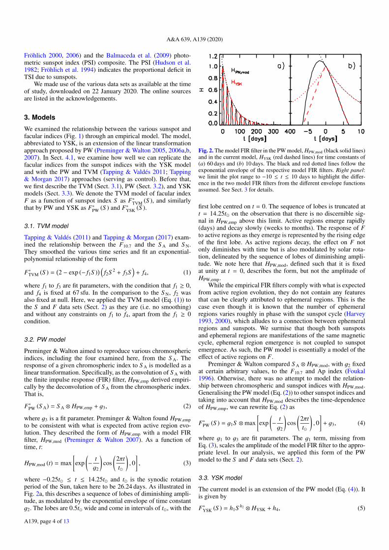
where −0.25t� ≤ t ≤ 14.25t� and t� is the synodic rotationperiod of the Sun, taken here to be 26.24 days. As illustrated inFig. 2a, this describes a sequence of lobes of diminishing ampli-tude, as modulated by the exponential envelope of time constantg2. The lobes are 0.5t� wide and come in intervals of t�, with the

Fig. 2. The model FIR filter in the PW model, HPW,mod (black solid lines)and in the current model, HYSK (red dashed lines) for time constants of(a) 60 days and (b) 10 days. The black and red dotted lines follow theexponential envelope of the respective model FIR filters. Right panel:we limit the plot range to −10 ≤ t ≤ 10 days to highlight the differ-ence in the two model FIR filters from the different envelope functionsassumed. See Sect. 3 for details.

first lobe centred on t = 0. The sequence of lobes is truncated att = 14.25t� on the observation that there is no discernible sig-nal in HPW,emp above this limit. Active regions emerge rapidly(days) and decay slowly (weeks to months). The response of Fto active regions as they emerge is represented by the rising edgeof the first lobe. As active regions decay, the effect on F notonly diminishes with time but is also modulated by solar rota-tion, delineated by the sequence of lobes of diminishing ampli-tude. We note here that HPW,mod, defined such that it is fixedat unity at t = 0, describes the form, but not the amplitude ofHPW,emp.

While the empirical FIR filters comply with what is expectedfrom active region evolution, they do not contain any featuresthat can be clearly attributed to ephemeral regions. This is thecase even though it is known that the number of ephemeralregions varies roughly in phase with the sunspot cycle (Harvey1993, 2000), which alludes to a connection between ephemeralregions and sunspots. We surmise that though both sunspotsand ephemeral regions are manifestations of the same magneticcycle, ephemeral region emergence is not coupled to sunspotemergence. As such, the PW model is essentially a model of theeffect of active regions on F.

Preminger & Walton compared S A ⊗ HPW,mod, with g2 fixedat certain arbitrary values, to the F10.7 and Ap index (Foukal1996). Otherwise, there was no attempt to model the relation-ship between chromospheric and sunspot indices with HPW,mod.Generalising the PW model (Eq. (2)) to other sunspot indices andtaking into account that HPW,mod describes the time-dependenceof HPW,emp, we can rewrite Eq. (2) as

F∗PW (S ) = g1S ⊗max[exp

(−

tg2

)cos

(2πtt�

), 0

]+ g3, (4)

where g1 to g3 are fit parameters. The g1 term, missing fromEq. (3), scales the amplitude of the model FIR filter to the appro-priate level. In our analysis, we applied this form of the PWmodel to the S and F data sets (Sect. 2).

3.3. YSK model

The current model is an extension of the PW model (Eq. (4)). Itis given by

F∗YSK (S ) = h1S h2 ⊗ HYSK + h4, (5)

A139, page 4 of 13

K. L. Yeo et al.: How faculae and network relate to sunspots

where

HYSK = max[exp

(−|t|h3

)cos

(2πtt�

), 0

], (6)

and h1 to h4 are fit parameters.The model FIR filter here, HYSK (Eq. (6)) is identical to that

in the PW model (Eq. (3)), except the exponential envelope isgiven by exp (−|t|/h3) instead of exp (−t/h3). The effect on themodel FIR filter is illustrated in Fig. 2b. While the envelopefunction adopted by PW skews the first lobe towards the negativetime domain (black solid line), the proposed envelope functionrenders it symmetrical at about t = 0 (red dashed line). We intro-duced this modification on the observation that the empirical FIRfilters derived by PW (see, for example, Fig. 1 in Preminger &Walton 2006a) do not indicate any clear skewness in the firstlobe at about t = 0.

In another departure from the PW model, the model FIR filteris applied to S h2 instead of S . By applying the FIR filter to S , thePW model implicitly assumes that, active region evolution aside,F scales linearly with S , which is unlikely to be the case. It isknown that chromospheric emission does not scale linearly withphotospheric magnetic flux density (e.g. Schrijver et al. 1989;Harvey & White 1999; Loukitcheva et al. 2009; Kahil et al.2017; Barczynski et al. 2018, see also Sect. 4.2) and facular areais a quadratic function of sunspot area (Foukal 1993, 1996, 1998;Chapman et al. 1997; Shapiro et al. 2014). This alludes to a non-linear relationship between plage emission and facular magneticflux, and between facular magnetic flux and S . We introducedthe h2 parameter to take this into account.

As noted in the introduction, Dudok de Wit et al. (2018) pre-sented a modified version of the PW model. In their model, thevariables are at 27-day (instead of daily) cadence so as to excludesolar rotation effects from the FIR filter. In addition, the g3 term(Eq. (2)) is allowed to vary with time. The authors found thatwith the coarser time resolution, most of the long-term (annualto decadal) variation in F is captured in g3(t) instead of the con-volution of S A and the FIR filter. We did not adopt these modifi-cations, as neither excluding solar rotation effects from the FIRfilter nor splitting the variability in F into two separate terms isnecessary for the purposes of the current study.

4. Analysis

4.1. Model validation

We modelled the relationship between each facular index, F andeach sunspot index, S . Taking each combination of F and S , wefitted the YSK model (Eqs. (5) and (6)) and the TVM (Eq. (1))and PW models (Eq. (4)), (serving as control). The fit parametersof the YSK model are listed in Table 1.

To validate the YSK model, we examined how well it repro-duces the facular indices from the sunspot indices as comparedto the two control models. For each model and each combina-tion of F and S , we derive the following. We calculate the devi-ation from unity of the Pearson’s correlation coefficient betweenF and the model reconstruction of F from S , F∗ (S ), denoted1 − R2. This quantity indicates the variability in F that is notreplicated in F∗ (S ). Taking the F-versus-F∗ (S ) scatter plot, wederive the ratio of the variance normal to and in the direction ofthe F = F∗ (S ) line, denoted as σ2

⊥/σ2‖. The more F∗ (S ) repli-

cates the variability and the scale of F, the lower the value ofσ2⊥/σ

2‖. To reveal how closely the long-term (annual to decadal)

trend in F is reproduced in F∗ (S ), we took the three-year run-ning mean of F and F∗ (S ), denoted as 〈F〉3Y and 〈F∗ (S )〉3Y,

Table 1. For each combination of F and S , the fit parameters of theYSK model (h1 to h4, Eqs. (5) and (6)).

F S h1 h2 h3 h4

F10.7 S A 0.1636 0.8603 24.35 64.38FCaIIK S A 1.129 × 10−4 0.5854 57.41 8.228 × 10−2

FLα S A 1.950 × 10−5 0.6642 72.34 5.852 × 10−3

FMgII S A 6.966 × 10−5 0.7129 54.10 0.1497Fφ S A 2.957 × 10−3 0.8429 33.46 0.1824F10.7 S N1 0.6212 1.073 13.41 65.10FCaIIK S N1 2.074 × 10−4 0.7913 34.84 8.243 × 10−2

FLα S N1 6.414 × 10−5 0.7960 49.25 5.861 × 10−3

FMgII S N1 2.385 × 10−4 0.8648 33.25 0.1498Fφ S N1 1.841 × 10−2 0.9572 20.15 0.1401F10.7 S N2 0.3876 1.092 13.42 65.44FCaIIK S N2 1.638 × 10−4 0.7846 34.52 8.254 × 10−2

FLα S N2 3.952 × 10−5 0.8346 46.47 5.898 × 10−3

FMgII S N2 1.298 × 10−4 0.9209 32.71 0.1501Fφ S N2 1.123 × 10−2 0.9841 20.26 0.1401F10.7 S G1 8.145 1.126 19.53 64.01FCaIIK S G1 8.831 × 10−4 0.9559 35.56 8.336 × 10−2

FLα S G1 3.237 × 10−4 0.9295 54.62 5.887 × 10−3

FMgII S G1 1.639 × 10−3 0.9539 31.37 0.1495Fφ S G1 0.1846 0.9538 23.28 0.1898F10.7 S G2 6.485 1.255 19.68 63.91FCaIIK S G2 1.181 × 10−3 0.9240 36.82 8.218 × 10−2

FLα S G2 3.064 × 10−4 1.002 48.40 5.850 × 10−3

FMgII S G2 1.244 × 10−3 1.105 34.04 0.1499Fφ S G2 0.1605 1.072 23.83 0.1279

Notes. See Sect. 4.1 for details.

and calculate the normalised residual, given by

〈F〉3Y − 〈F∗ (S )〉3Y

〈F〉3Y,2000 − 〈F〉3Y,2008· (7)

This is the difference between 〈F〉3Y and 〈F∗ (S )〉3Y, normalisedto the change in the former between the 2000 solar cycle max-imum and 2008 minimum. Following convention, the epoch ofsolar cycle extrema is taken from the 13-month moving meanof the monthly S N2. The normalisation expresses the residual asa proportion of solar cycle variability. The discrepancy betweenthe measured and modelled long-term variability is also encapsu-lated in the root-mean-square of the normalised residual, abbre-viated as RMSNR. We tabulate 1 − R2, σ2

⊥/σ2‖

and RMSNR inTable 2, and depict the normalised residue of the YSK model inFig. 3.

For the YSK model, 1 − R2 ranges from about 0.06 to 0.18and RMSNR from 0.02 to 0.08 (Table 2), indicating that it repro-duces about 82% to 94% of the variability in the various facularindices and their long-term trend to about 2% to 8% of solarcycle variability. In terms of 1 − R2, σ2

⊥/σ2‖

and RMSNR, theYSK and PW models replicate the facular indices better than theTVM model. The only exceptions are the FMgII & S N1 and FLα& S N1 analyses, where only the YSK model registered a lowerRMSNR than the TVM model. The strength of the YSK and PWmodels over the TVM model highlights how important it is, insuch studies, to account for the fact that active region magneticfluxes decay slower than sunspots (as similarly argued by Foukal1998; Preminger & Walton 2007), and the suitability of the lin-ear transformation approach proposed by PW for this purpose.

A139, page 5 of 13

A&A 639, A139 (2020)

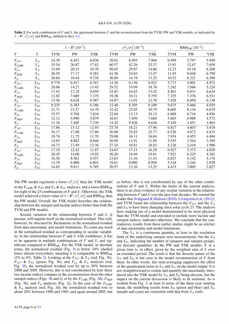
Table 2. For each combination of F and S , the agreement between F and the reconstruction from the TVM, PW and YSK models, as indicated by1 − R2, σ2

⊥/σ2‖

and RMSNR, defined in Sect. 4.1.

1 − R2 [10−2] σ2⊥/σ

2‖

[10−3] RMSNR [10−2]

F S TVM PW YSK TVM PW YSK TVM PW YSK

F10.7 S A 14.30 6.453 6.036 20.01 8.493 7.904 6.599 5.797 5.949FCaIIK S A 35.54 26.87 17.62 60.57 42.26 25.37 13.91 12.67 7.659FLα S A 31.09 20.15 10.78 50.65 29.87 14.66 12.23 10.18 6.209FMgII S A 26.55 17.17 9.283 41.50 24.83 12.47 11.93 9.848 6.799Fφ S A 20.84 10.44 9.728 30.88 14.19 13.25 10.52 6.321 6.390F10.7 S N1 9.779 6.917 6.767 13.20 9.136 8.922 5.773 4.901 4.972FCaIIK S N1 20.06 14.27 13.45 29.52 19.99 18.70 7.242 7.084 5.224FLα S N1 17.92 12.18 9.659 25.87 16.83 13.02 8.401 8.831 6.634FMgII S N1 13.82 7.689 7.375 19.28 10.21 9.759 7.335 7.376 6.531Fφ S N1 13.56 9.628 9.587 18.87 13.01 12.78 7.428 6.050 6.138F10.7 S N2 9.235 6.383 6.186 12.40 8.395 8.109 9.675 5.466 4.929FCaIIK S N2 21.71 15.57 14.79 32.42 22.05 20.79 8.605 8.134 6.679FLα S N2 15.57 9.704 7.634 22.04 13.13 10.12 6.868 6.716 4.856FMgII S N2 12.12 5.990 5.879 16.67 7.850 7.688 5.683 4.988 4.572Fφ S N2 11.29 7.405 7.370 15.42 9.826 9.638 5.450 3.851 3.963F10.7 S G1 17.86 13.12 12.93 25.78 18.21 17.90 6.817 4.603 3.418FCaIIK S G1 24.17 17.88 17.86 36.90 25.83 25.77 6.526 4.872 4.833FLα S G1 19.76 11.75 11.70 29.00 16.11 16.04 7.934 4.455 4.484FMgII S G1 14.85 8.882 8.848 20.90 11.91 11.85 5.555 3.544 3.399Fφ S G1 18.73 13.49 13.36 27.24 18.81 18.83 4.126 2.416 1.996F10.7 S G2 17.19 12.42 11.87 24.67 17.13 16.29 6.927 5.373 4.030FCaIIK S G2 20.45 14.08 14.03 30.20 19.69 19.61 7.921 6.225 4.382FLα S G2 16.56 8.561 8.557 23.63 11.44 11.43 6.823 4.142 4.176FMgII S G2 13.39 6.890 6.801 18.61 9.090 8.958 5.518 3.244 2.929Fφ S G2 14.65 9.811 9.785 20.57 13.26 13.25 4.433 2.005 2.027

The PW model registered a lower σ2⊥/σ

2‖

than the YSK modelin the FCaIIK & S N2 and Fφ & S G1 analyses, and a lower RMSNRfor eight of the 25 combinations of F and S . Otherwise, the YSKmodel achieved a lower value of 1−R2, σ2

⊥/σ2‖

and RMSNR thanthe PW model. Overall, the YSK model describes the relation-ship between the sunspot and facular indices better than both theTVM and PW models.

Secular variation in the relationship between F and S , ifpresent, will imprint itself on the normalised residual. This will,however, be obscured by fluctuations in the normalised residualfrom data uncertainty and model limitations. To count any trendin the normalised residual as corresponding to secular variabil-ity in the relationship between F and S with confidence, it hasto be apparent in multiple combinations of F and S , and sig-nificant compared to RMSNR. For the YSK model, in absoluteterms, the normalised residual (Fig. 3) is below 10% (dashedlines) almost everywhere, meaning it is comparable to RMSNR(2% to 8%, Table 2). Looking at the F10.7 & S A (red, Fig. 3b),F10.7 & S N1 (green, Fig. 3b), and FLα & S A analyses (red,Fig. 3f), the normalised residual rose by up to 20% between2000 and 2005. However, this is not corroborated by how thesetwo facular indices compare to the reconstruction from the othersunspot indices (Figs. 3b and f), or by the FCaIIK (Fig. 3d), FMgII(Fig. 3h), and Fφ analyses (Fig. 3j). In the case of the FCaIIK& S A analysis (red, Fig. 3d), the normalised residual rose toabout 20% between 1980 and 1985, and again around 2005, but

as before, this is not corroborated by any of the other combi-nations of F and S . Within the limits of the current analysis,there is no clear evidence of any secular variation in the relation-ship between F and S over the past four decades. We remind thereader that Svalgaard & Hudson (2010), Livingston et al. (2012),and TVM found the relationship between the F10.7 and the S Aand S N to have been changing since solar cycle 23. The analysishere, making use of a model demonstrated to be more physicalthan the TVM model and extended to include more facular andsunspot indices, indicates otherwise. We conclude that the con-tradictory results from these earlier studies might be an artefactof data uncertainty and model limitations.

The S A is a continuous quantity, at least to the resolutionlimit of the underlying sunspot area measurements, but the S Nand S G, indicating the number of sunspots and sunspot groups,are discrete quantities. In the PW and YSK models, F at agiven time is, in effect, given by the weighted sum of S overan extended period. The result is that the discrete nature of theS N and S G is not seen in the model reconstruction of F fromthem. In other words, this time-averaging suppresses the effectof the quantization noise in S N and S G on the model output. It isnot straightforward to isolate and quantify the uncertainty intro-duced into the YSK model by S N and S G being discrete, but theimpact on the current discussion is likely to be minimal. As isevident from Fig. 3, at least in terms of the three-year runningmean, the modelling results from S N (green and blue) and S G(purple and cyan) are consistent with that from S A (red).

A139, page 6 of 13

K. L. Yeo et al.: How faculae and network relate to sunspots

Fig. 3. a: three-year running mean of F10.7 (black) and the YSK modelreconstruction of this facular index from the S A (red), S N1 (green), S N2(blue), S G1 (purple), and S G2 (cyan). b: residual between the observedand reconstructed time series, normalised to the change in the formerbetween the 2000 solar cycle maximum and 2008 minimum (Eq. (7)).The dashed lines mark the 10% bound. c–j: The corresponding plots forthe FCaIIK, FLα, FMgII and Fφ.

4.2. How faculae and network relate to sunspots

As noted in the introduction, the amount of faculae and networkpresent on the solar disc at a given time is not indicated by pre-vailing sunspots alone due to how active regions evolve and the

contribution by ephemeral regions and the internetwork mag-netic field. In the YSK model, F∗YSK (S ), active region evolutionis taken into account by the convolution of the sunspot indices, Swith the model FIR filter, HYSK (Eqs. (5) and (6)). So whether inmeasurements or in the YSK model, a particular level of S doesnot map to a unique value of F. Nonetheless, we can still gaininsight into how faculae and network relate to sunspots by look-ing at the overall trend in F with S . To this end, we comparedthe amplitude of the solar cycle in F∗YSK (S ) and S . We optedto compare F∗YSK (S ) instead of the measured F to S because ofthe following considerations. Since the S time series go furtherback in time than the F time series (Fig. 1), and F∗YSK (S ) evi-dently extend as far as S , we can compare F∗YSK (S ) and S overlonger periods than when comparing F and S . More critically,how the cycle amplitude in F and S compare can be affected bythe uncertainty in the decadal trend in the various time series.This uncertainty is irrelevant when comparing F∗YSK (S ) and S .We recognise that the comparison of F∗YSK (S ) and S is onlyvalid as far as the YSK model is physical, but the robustness ofthe model, demonstrated in Sect. 4.1, renders confidence in thisapproach. The S A is a more direct measure of sunspot prevalencethan the S N and S G, which give sunspots and sunspot groups ofdifferent areas the same weighting. With this in mind, the focushere is on how F∗YSK (S A) and S A compare.

We use ∆F as an abbreviation of the deviation in F fromthe 2008 solar cycle minimum level. Here, we define the cycleamplitude of F and S , which we denote as A (F) and A (S ), as thevalue of the three-year running mean of ∆F and S at cycle max-ima. In Fig. 4, we chart A

(F∗YSK (S A)

)/A (S A) against A (S A)

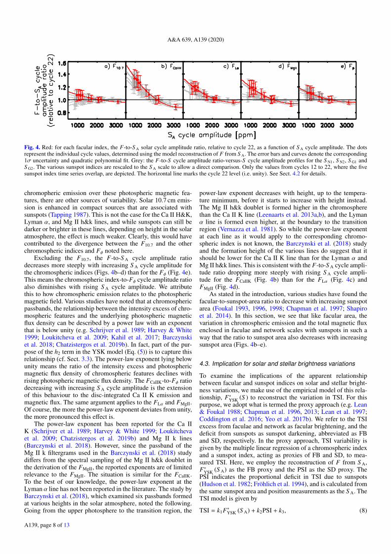
(red), revealing the trend in the F-to-S A cycle amplitude ratiowith S A cycle amplitude as indicated by the YSK model. Tocompare the results from the various facular indices, we nor-malised the F-to-S A cycle amplitude ratio from each index to thecycle 22 value. The uncertainty in the F-to-S A cycle amplituderatio, marked in the figure, is propagated from the uncertainty inthe long-term trend in F∗YSK (S ), RMSNR (Table 2). For the vari-ous facular indices, the F-to-S A cycle amplitude ratio decreaseswith increasing S A cycle amplitude (Fig. 4). The decline is steep-est for the FCaIIK (Fig. 4b), followed by the FLα and FMgII (wherethe trend with S A cycle amplitude is closely similar, Figs. 4c,d),then the Fφ (Fig. 4e), and finally the F10.7 (Fig. 4a). For the F10.7,the trend is weak in relation to the uncertainty.

As a check, we repeated the above analysis with F∗YSK (S N1)and S N1, that is, we examined A

(F∗YSK (S N1)

)/A (S N1) as a func-

tion of A (S N1). To allow a direct comparison to the F∗YSK (S A)and S A analysis, A (S N1) is calculated after rescaling this sunspotindex to the scale of the S A using the quadratic polynomial fit tothe S A-versus-S N1 scatter plot. This is repeated for F∗YSK (S N2)and S N2, F∗YSK (S G1) and S G1, and F∗YSK (S G2) and S G2. Theresults are drawn in grey in Fig. 4. The A

(F∗YSK (S )

)/A (S )-

versus-A (S ) profiles from the various sunspot indices lie largelywithin 1σ of one another, indicating that they are mutually con-sistent, affirming what we noted with the F∗YSK (S A) and S A anal-ysis (red). Notably, for the F10.7 (Fig. 4a), while the various pro-files are within error of one another, they indicate conflictingtrends with S A cycle amplitude. In other words, for this partic-ular facular index, the underlying trend is too weak to be estab-lished by the current analysis.

The observation here that the F10.7 departs from the otherfacular indices in terms how it compares to the S A is at leastpartly due to the following. We noted in the introduction thatwhile the various chromospheric indices are strongly modulatedby faculae and network prevalence due to the enhancement of

A139, page 7 of 13

A&A 639, A139 (2020)

Fig. 4. Red: for each facular index, the F-to-S A solar cycle amplitude ratio, relative to cycle 22, as a function of S A cycle amplitude. The dotsrepresent the individual cycle values, determined using the model reconstruction of F from S A. The error bars and curves denote the corresponding1σ uncertainty and quadratic polynomial fit. Grey: the F-to-S cycle amplitude ratio-versus-S cycle amplitude profiles for the S N1, S N2, S G1 andS G2. The various sunspot indices are rescaled to the S A scale to allow a direct comparison. Only the values from cycles 12 to 22, where the fivesunspot index time series overlap, are depicted. The horizontal line marks the cycle 22 level (i.e. unity). See Sect. 4.2 for details.

chromopheric emission over these photospheric magnetic fea-tures, there are other sources of variability. Solar 10.7 cm emis-sion is enhanced in compact sources that are associated withsunspots (Tapping 1987). This is not the case for the Ca II H&K,Lyman α, and Mg II h&k lines, and while sunspots can still bedarker or brighter in these lines, depending on height in the solaratmosphere, the effect is much weaker. Clearly, this would havecontributed to the divergence between the F10.7 and the otherchromospheric indices and Fφ noted here.

Excluding the F10.7, the F-to-S A cycle amplitude ratiodecreases more steeply with increasing S A cycle amplitude forthe chromospheric indices (Figs. 4b–d) than for the Fφ (Fig. 4e).This means the chromospheric index-to-Fφ cycle amplitude ratioalso diminishes with rising S A cycle amplitude. We attributethis to how chromospheric emission relates to the photosphericmagnetic field. Various studies have noted that at chromosphericpassbands, the relationship between the intensity excess of chro-mospheric features and the underlying photospheric magneticflux density can be described by a power law with an exponentthat is below unity (e.g. Schrijver et al. 1989; Harvey & White1999; Loukitcheva et al. 2009; Kahil et al. 2017; Barczynskiet al. 2018; Chatzistergos et al. 2019b). In fact, part of the pur-pose of the h2 term in the YSK model (Eq. (5)) is to capture thisrelationship (cf. Sect. 3.3). The power-law exponent lying belowunity means the ratio of the intensity excess and photosphericmagnetic flux density of chromospheric features declines withrising photospheric magnetic flux density. The FCaIIK-to-Fφ ratiodecreasing with increasing S A cycle amplitude is the extensionof this behaviour to the disc-integrated Ca II K emission andmagnetic flux. The same argument applies to the FLα and FMgII.Of course, the more the power-law exponent deviates from unity,the more pronounced this effect is.

The power-law exponent has been reported for the Ca IIK (Schrijver et al. 1989; Harvey & White 1999; Loukitchevaet al. 2009; Chatzistergos et al. 2019b) and Mg II k lines(Barczynski et al. 2018). However, since the passband of theMg II k filtergrams used in the Barczynski et al. (2018) studydiffers from the spectral sampling of the Mg II h&k doublet inthe derivation of the FMgII, the reported exponents are of limitedrelevance to the FMgII. The situation is similar for the FCaIIK.To the best of our knowledge, the power-law exponent at theLyman α line has not been reported in the literature. The study byBarczynski et al. (2018), which examined six passbands formedat various heights in the solar atmosphere, noted the following.Going from the upper photosphere to the transition region, the

power-law exponent decreases with height, up to the tempera-ture minimum, before it starts to increase with height instead.The Mg II h&k doublet is formed higher in the chromospherethan the Ca II K line (Leenaarts et al. 2013a,b), and the Lymanα line is formed even higher, at the boundary to the transitionregion (Vernazza et al. 1981). So while the power-law exponentat each line as it would apply to the corresponding chromo-spheric index is not known, the Barczynski et al. (2018) studyand the formation height of the various lines do suggest that itshould be lower for the Ca II K line than for the Lyman α andMg II h&k lines. This is consistent with the F-to-S A cycle ampli-tude ratio dropping more steeply with rising S A cycle ampli-tude for the FCaIIK (Fig. 4b) than for the FLα (Fig. 4c) andFMgII (Fig. 4d).

As stated in the introduction, various studies have found thefacular-to-sunspot-area ratio to decrease with increasing sunspotarea (Foukal 1993, 1996, 1998; Chapman et al. 1997; Shapiroet al. 2014). In this section, we see that like facular area, thevariation in chromospheric emission and the total magnetic fluxenclosed in faculae and network scales with sunspots in such away that the ratio to sunspot area also decreases with increasingsunspot area (Figs. 4b–e).

4.3. Implication for solar and stellar brightness variations

To examine the implications of the apparent relationshipbetween facular and sunspot indices on solar and stellar bright-ness variations, we make use of the empirical model of this rela-tionship, F∗YSK (S ) to reconstruct the variation in TSI. For thispurpose, we adopt what is termed the proxy approach (e.g. Lean& Foukal 1988; Chapman et al. 1996, 2013; Lean et al. 1997;Coddington et al. 2016; Yeo et al. 2017b). We refer to the TSIexcess from faculae and network as facular brightening, and thedeficit from sunspots as sunspot darkening, abbreviated as FBand SD, respectively. In the proxy approach, TSI variability isgiven by the multiple linear regression of a chromospheric indexand a sunspot index, acting as proxies of FB and SD, to mea-sured TSI. Here, we employ the reconstruction of F from S A,F∗YSK (S A) as the FB proxy and the PSI as the SD proxy. ThePSI indicates the proportional deficit in TSI due to sunspots(Hudson et al. 1982; Fröhlich et al. 1994), and is calculated fromthe same sunspot area and position measurements as the S A. TheTSI model is given by

TSI = k1F∗YSK (S A) + k2PSI + k3, (8)

A139, page 8 of 13

K. L. Yeo et al.: How faculae and network relate to sunspots

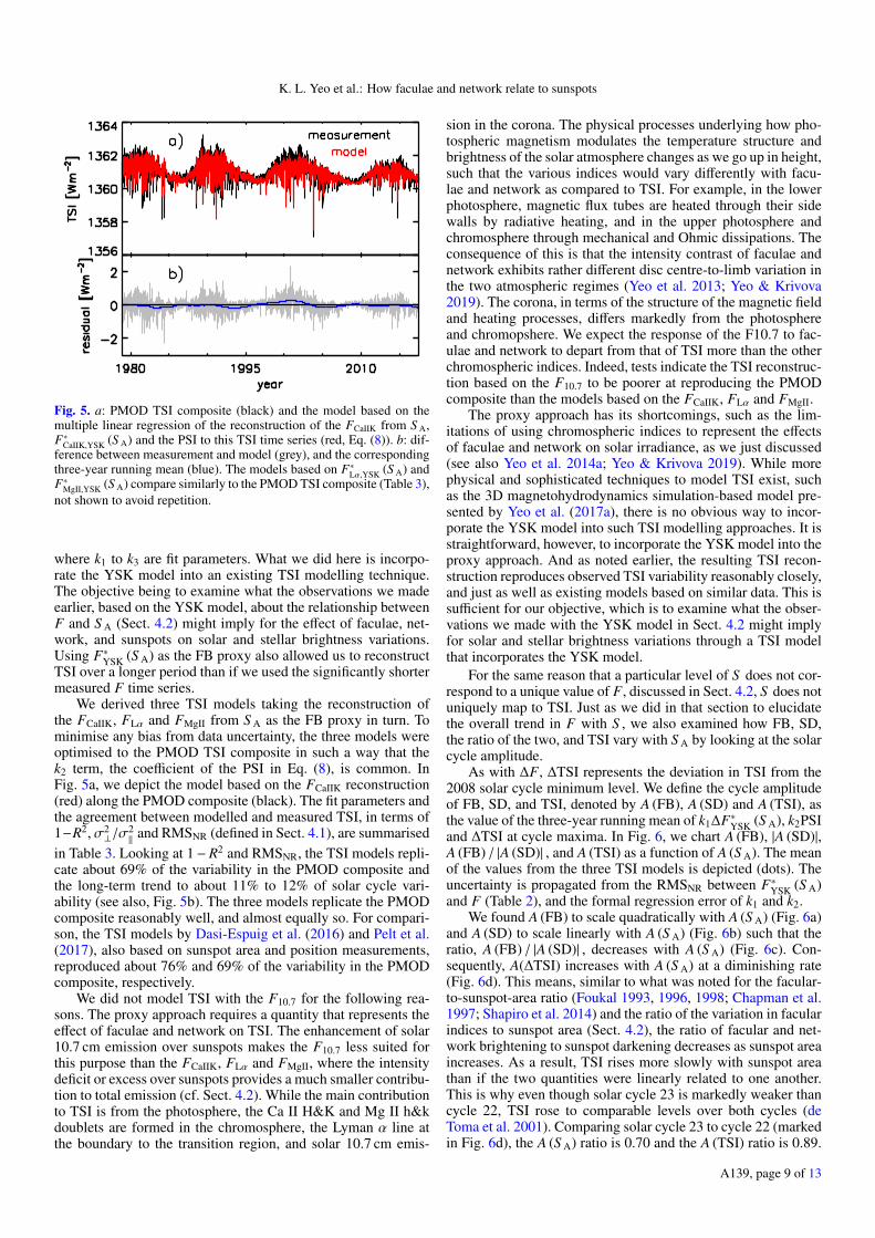
Fig. 5. a: PMOD TSI composite (black) and the model based on themultiple linear regression of the reconstruction of the FCaIIK from S A,F∗CaIIK,YSK (S A) and the PSI to this TSI time series (red, Eq. (8)). b: dif-ference between measurement and model (grey), and the correspondingthree-year running mean (blue). The models based on F∗Lα,YSK (S A) andF∗MgII,YSK (S A) compare similarly to the PMOD TSI composite (Table 3),not shown to avoid repetition.

where k1 to k3 are fit parameters. What we did here is incorpo-rate the YSK model into an existing TSI modelling technique.The objective being to examine what the observations we madeearlier, based on the YSK model, about the relationship betweenF and S A (Sect. 4.2) might imply for the effect of faculae, net-work, and sunspots on solar and stellar brightness variations.Using F∗YSK (S A) as the FB proxy also allowed us to reconstructTSI over a longer period than if we used the significantly shortermeasured F time series.

We derived three TSI models taking the reconstruction ofthe FCaIIK, FLα and FMgII from S A as the FB proxy in turn. Tominimise any bias from data uncertainty, the three models wereoptimised to the PMOD TSI composite in such a way that thek2 term, the coefficient of the PSI in Eq. (8), is common. InFig. 5a, we depict the model based on the FCaIIK reconstruction(red) along the PMOD composite (black). The fit parameters andthe agreement between modelled and measured TSI, in terms of1−R2, σ2

⊥/σ2‖

and RMSNR (defined in Sect. 4.1), are summarisedin Table 3. Looking at 1− R2 and RMSNR, the TSI models repli-cate about 69% of the variability in the PMOD composite andthe long-term trend to about 11% to 12% of solar cycle vari-ability (see also, Fig. 5b). The three models replicate the PMODcomposite reasonably well, and almost equally so. For compari-son, the TSI models by Dasi-Espuig et al. (2016) and Pelt et al.(2017), also based on sunspot area and position measurements,reproduced about 76% and 69% of the variability in the PMODcomposite, respectively.

We did not model TSI with the F10.7 for the following rea-sons. The proxy approach requires a quantity that represents theeffect of faculae and network on TSI. The enhancement of solar10.7 cm emission over sunspots makes the F10.7 less suited forthis purpose than the FCaIIK, FLα and FMgII, where the intensitydeficit or excess over sunspots provides a much smaller contribu-tion to total emission (cf. Sect. 4.2). While the main contributionto TSI is from the photosphere, the Ca II H&K and Mg II h&kdoublets are formed in the chromosphere, the Lyman α line atthe boundary to the transition region, and solar 10.7 cm emis-

sion in the corona. The physical processes underlying how pho-tospheric magnetism modulates the temperature structure andbrightness of the solar atmosphere changes as we go up in height,such that the various indices would vary differently with facu-lae and network as compared to TSI. For example, in the lowerphotosphere, magnetic flux tubes are heated through their sidewalls by radiative heating, and in the upper photosphere andchromosphere through mechanical and Ohmic dissipations. Theconsequence of this is that the intensity contrast of faculae andnetwork exhibits rather different disc centre-to-limb variation inthe two atmospheric regimes (Yeo et al. 2013; Yeo & Krivova2019). The corona, in terms of the structure of the magnetic fieldand heating processes, differs markedly from the photosphereand chromopshere. We expect the response of the F10.7 to fac-ulae and network to depart from that of TSI more than the otherchromospheric indices. Indeed, tests indicate the TSI reconstruc-tion based on the F10.7 to be poorer at reproducing the PMODcomposite than the models based on the FCaIIK, FLα and FMgII.

The proxy approach has its shortcomings, such as the lim-itations of using chromospheric indices to represent the effectsof faculae and network on solar irradiance, as we just discussed(see also Yeo et al. 2014a; Yeo & Krivova 2019). While morephysical and sophisticated techniques to model TSI exist, suchas the 3D magnetohydrodynamics simulation-based model pre-sented by Yeo et al. (2017a), there is no obvious way to incor-porate the YSK model into such TSI modelling approaches. It isstraightforward, however, to incorporate the YSK model into theproxy approach. And as noted earlier, the resulting TSI recon-struction reproduces observed TSI variability reasonably closely,and just as well as existing models based on similar data. This issufficient for our objective, which is to examine what the obser-vations we made with the YSK model in Sect. 4.2 might implyfor solar and stellar brightness variations through a TSI modelthat incorporates the YSK model.

For the same reason that a particular level of S does not cor-respond to a unique value of F, discussed in Sect. 4.2, S does notuniquely map to TSI. Just as we did in that section to elucidatethe overall trend in F with S , we also examined how FB, SD,the ratio of the two, and TSI vary with S A by looking at the solarcycle amplitude.

As with ∆F, ∆TSI represents the deviation in TSI from the2008 solar cycle minimum level. We define the cycle amplitudeof FB, SD, and TSI, denoted by A (FB), A (SD) and A (TSI), asthe value of the three-year running mean of k1∆F∗YSK (S A), k2PSIand ∆TSI at cycle maxima. In Fig. 6, we chart A (FB), |A (SD)|,A (FB) / |A (SD)| , and A (TSI) as a function of A (S A). The meanof the values from the three TSI models is depicted (dots). Theuncertainty is propagated from the RMSNR between F∗YSK (S A)and F (Table 2), and the formal regression error of k1 and k2.

We found A (FB) to scale quadratically with A (S A) (Fig. 6a)and A (SD) to scale linearly with A (S A) (Fig. 6b) such that theratio, A (FB) / |A (SD)| , decreases with A (S A) (Fig. 6c). Con-sequently, A(∆TSI) increases with A (S A) at a diminishing rate(Fig. 6d). This means, similar to what was noted for the facular-to-sunspot-area ratio (Foukal 1993, 1996, 1998; Chapman et al.1997; Shapiro et al. 2014) and the ratio of the variation in facularindices to sunspot area (Sect. 4.2), the ratio of facular and net-work brightening to sunspot darkening decreases as sunspot areaincreases. As a result, TSI rises more slowly with sunspot areathan if the two quantities were linearly related to one another.This is why even though solar cycle 23 is markedly weaker thancycle 22, TSI rose to comparable levels over both cycles (deToma et al. 2001). Comparing solar cycle 23 to cycle 22 (markedin Fig. 6d), the A (S A) ratio is 0.70 and the A (TSI) ratio is 0.89.

A139, page 9 of 13

A&A 639, A139 (2020)

Table 3. The fit parameters of the empirical TSI models (k1 to k3, Eq. (8)) derived taking the reconstruction of the FCaIIK, FLα and FMgII from S A,denoted F∗CaIIK,YSK (S A), F∗Lα,YSK (S A) and F∗MgII,YSK (S A), as the FB proxy (i.e. the proxy of the TSI excess from faculae and network).

FB proxy k1 k2 k3 1 − R2 σ2⊥/σ

2‖

[10−2] RMSNR

F∗CaIIK,YSK (S A) 209.0 10.36 1343.09 0.3072 4.954 0.1102F∗Lα,YSK (S A) 643.8 10.36 1356.58 0.3014 4.785 0.1152F∗MgII,YSK (S A) 119.1 10.36 1342.57 0.3088 5.173 0.1106

Notes. The various models are optimised to the PMOD TSI composite in such a way that k2 is identical. The agreement between model andmeasurement in terms of 1 − R2, σ2

⊥/σ2‖

and RMSNR, defined in Sect. 4.1, is also tabulated.

Fig. 6. From top to bottom: as a function of S A cycle amplitude, thecycle amplitude of (a) the effect of faculae and network (red), and (b)of sunspots on TSI (blue), (c) the ratio of the two (green), and (d) TSI(black). That is, A (FB), |A (SD)|, A (FB) / |A (SD)|, and A (TSI)-versus-A (S A). The plot points and error bars represent the mean of the val-ues from the three TSI models and the associated 1σ uncertainty (seeSect. 4.3). The latter is omitted in the case of A (FB) and A (SD), whereit is so minute as to be obscured by the plot points. The values from theindividual TSI models, lying within 1σ of the mean, are not drawn toavoid cluttering. The S A and PSI time series on which the TSI modelsare based, and therefore the plot points, cover solar cycles 12 to 24. TheA (TSI) plot points corresponding to solar cycles 22 and 23 are labelled.The lines correspond to the linear or quadratic polynomial fit.

Due to the non-linear relationship between TSI and sunspot area,while cycle 23 is, in terms of S A, 30% weaker than cycle 22, theTSI cycle amplitude is only 11% weaker.

We remind the reader that for Sun-like stars, going above acertain level of activity, they switch from growing brighter withrising activity to becoming dimmer instead, which is interpretedas the transition from a faculae-dominated to a spot-dominatedregime (Lockwood et al. 2007; Hall et al. 2009; Shapiro et al.2014; Radick et al. 2018). The Sun appears to be just belowthis transition, opening up the possibility of studying this phe-nomena by looking at how solar faculae and network relate tosunspots, and extrapolating the apparent relationship to higher

Fig. 7. Cycle amplitude of FB (red plot points), SD (blue) and TSI(black), taken from Fig. 6, as a function of log R′HK. The corresponding1σ uncertainty, not drawn, is generally much smaller than the plot sym-bols. The red line follows the linear fit to A (FB) and the blue line thequadratic fit to |A (SD)|, while the black line indicates the correspondingA (TSI) level. The shaded region encloses the 95% confidence intervalof the A (TSI) curve. The dashed lines mark the turning point of theA (TSI) curve and the dotted lines where it goes below zero, denoted T1and T2, respectively. See Sect. 4.3 for the physical interpretation. Theboxed area is blown up in the bottom panel.

activity levels. We attempt exactly that here by projecting theTSI model, which is based on the empirical model of the rela-tionship between facular and sunspot indices, to higher activitylevels.

We had examined A (FB), |A (SD)|, A (FB) / |A (SD)| , andA (TSI) as a function of activity as indicated by A (S A) (Fig. 6).In the stellar studies, activity is characterised by the log R′HK.Accordingly, we converted F∗CaIIK,YSK (S A) to the S -index scale(not to be confused with sunspot indices, abbreviated as Sin this article) using the conversion relationship reported byEgeland et al. (2017), and then the result to log R′HK follow-ing the procedure of Noyes et al. (1984). In this computation,we assumed a solar (B − V) colour index of 0.653 (Ramírezet al. 2012). In Fig. 7, we plot A (FB) (red dots), |A (SD)| (bluedots) and A (TSI) (black dots) again, this time as a functionof log R′HK. The log R′HK level corresponding to each A (FB),

A139, page 10 of 13

K. L. Yeo et al.: How faculae and network relate to sunspots

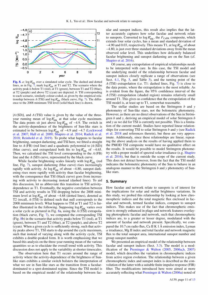
Fig. 8. a: log R′HK over a simulated solar cycle. The dashed and dottedlines, as in Fig. 7, mark log R′HK at T1 and T2. The scenario where theactivity peak is below T1 (red), at T1 (green), between T1 and T2 (blue),at T2 (purple) and above T2 (cyan) are depicted. b: TSI correspondingto each scenario, similarly colour-coded, as given by the empirical rela-tionship between A (TSI) and log R′HK (black curve, Fig. 7). The differ-ence to the 2008 minimum TSI level (solid black line) is drawn.

|A (SD)|, and A (TSI) value is given by the value of the three-year running mean of log R′HK at that solar cycle maximum.The data points sit just above log R′HK of −4.9. The switch inthe activity-dependence of the brightness of Sun-like stars isestimated to be between log R′HK of −4.9 and −4.7 (Lockwoodet al. 2007; Hall et al. 2009; Shapiro et al. 2014; Radick et al.2018; Reinhold et al. 2019). To probe what happens to facularbrightening, sunspot darkening, and TSI here, we fitted a straightline to A (FB) (red line) and a quadratic polynomial to |A (SD)|(blue curve), and extrapolated both fits to log R′HK of −4.65.Then, we calculated the TSI level corresponding to the A (FB)line and the A (SD) curve, represented by the black curve.

While facular brightening scales linearly with log R′HK (redline, Fig. 7), sunspot darkening (blue curve) rises increasinglyrapidly with activity. At log R′HK of about −4.80, sunspot dark-ening rises more rapidly with activity than facular brightening,with the consequence that TSI (black curve) goes from increas-ing with activity to decreasing instead (dashed lines). To aidthis discussion, let us abbreviate this transition in TSI activity-dependence as T1. Eventually, the negative correlation betweenTSI and activity results in TSI dropping below the 2008 mini-mum level at log R′HK of about −4.68 (dotted lines), denoted asT2 (recall, A (TSI) is defined such that null corresponds to the2008 minimum level). What happens to TSI at T1 and T2 is fur-ther illustrated in the following. Supposing log R′HK varies overa solar cycle as pictured in Fig. 8a, using the A (TSI) extrapola-tion (black curve, Fig. 7), we computed the corresponding TSI(Fig. 8b) in the scenario that activity peaks below T1 (red), at T1(green), between T1 and T2 (blue), at T2 (purple), and above T2(cyan). When a given cycle is sufficiently strong, such that activ-ity peaks above T1, TSI starts to dip around the cycle maximum,such that instead of varying along with the activity cycle, TSIexhibits a double-peaked form. It is worth emphasising that webased this analysis on the three-year running mean of the variousquantities so as to elucidate the overall trend with activity. Thisdiscussion does not apply to the variability at shorter timescales.

The observation here that T1 occurs around the range ofactivity where the activity-dependence of the brightness of Sun-like stars exhibits a similar switch bolsters the interpretation ofwhat we see in Sun-like stars as the transition from a faculae-dominated to a spot-dominated regime. Since the TSI model isbased on the empirical model of the relationship between fac-

ular and sunspot indices, this result also implies that the lat-ter accurately captures how solar faculae and network relateto sunspots. Converted to log R′HK, the FCaIIK composite, whichextends four solar cycles, has a mean and standard deviation of−4.90 and 0.03, respectively. This means T1, at log R′HK of about−4.80, is just over three standard deviations away from the meanobserved solar level. This underlines how delicately balancedfacular brightening and sunspot darkening are on the Sun (cf.Shapiro et al. 2016).

Of course, any extrapolation of empirical relationships needsto be interpreted with care. In this case, the TSI model andthe underlying model of the relationship between facular andsunspot indices closely replicate a range of observations (seeSect. 4.1, Fig. 5, and Table 3), and the turning point of theA (TSI) extrapolation (i.e. T1: dashed lines, Fig. 7) is close tothe data points, where the extrapolation is the most reliable. Asis evident from the figure, the 95% confidence interval of theA (TSI) extrapolation (shaded region) remains relatively smallaround T1. This gives us confidence that the extrapolation of theTSI model is, at least up to T1, somewhat reasonable.

The stellar studies are based on the Strömgren b and yphotometry of Sun-like stars, not the bolometric photometry.However, as there are no direct observations of the Sun in Ström-gren b and y, deriving an empirical model of solar Strömgren band y as we did for TSI is currently not possible. This is a limita-tion of the current model. Studies have reported linear relation-ships for converting TSI to solar Strömgren b and y (see Radicket al. 2018 and references therein), but these are very approx-imate. Additionaly, since these relationships are linear, repeat-ing the above analysis on the results of having applied them tothe PMOD TSI composite would have no qualitative effect onthe results. It would be possible to model Strömgren photome-try with a proper model of spectral solar irradiance (e.g. Shapiroet al. 2016), but that is outside the scope of the current study.This does not detract however, from the fact that the TSI modelindicates the bolometric photometry of the Sun to behave in ananalogous manner to the Strömgren b and y photometry of Sun-like stars.

5. Summary

How faculae and network relate to sunspots is of interest forthe implications for solar and stellar brightness variations. Inthis study, we probed this relationship by looking at how chro-mospheric indices and the total magnetic flux enclosed in fac-ulae and network, termed faculae indices, compare to sunspotindices. This makes use of the fact that chromospheric emis-sion is strongly enhanced in plage and network features overlay-ing photospheric faculae and network, such that chromosphericindices are, to a greater or lesser degree, modulated with theamount of faculae and network present. Specifically, we com-pared the 10.7 cm radio flux, Ca II K 1 Å emission index, Lymanα irradiance, Mg II index and total facular and network magneticflux to the total sunspot area, international sunspot number andgroup sunspot number.

We presented an empirical model of the relationship betweenfacular and sunspot indices (Sect. 3.3). The model is a mod-ification of the Preminger & Walton (2005, 2006a,b, 2007)model, which describes the variation in chromospheric indicesfrom active region evolution. The relationship between a givenchromospheric index and sunspot index is described as the con-volution of the latter with a suitable finite impulse response (FIR)filter. The modifications introduced here were aimed at moreaccurately reflecting what Preminger & Walton (2006a) noted of

A139, page 11 of 13

A&A 639, A139 (2020)

the FIR filters they had derived empirically from observations,and also to take into account the likely non-linear relationshipbetween plage emission and facular magnetic flux, and betweenthe latter and sunspot prevalence. Taking the current model, wereconstructed the facular indices from the sunspot indices. Themodel not only replicated most of the observed variability (upto 94%), but it is also better at doing so than the Preminger &Walton (2005, 2006a,b, 2007) model, as well as that of Tapping& Valdés (2011) and Tapping & Morgan (2017) (Sect. 4.1).

Tapping & Valdés (2011) and Tapping & Morgan (2017),along with Svalgaard & Hudson (2010) and Livingston et al.(2012), found the relationship between the 10.7 cm radio fluxand the total sunspot area and international sunspot number tohave changed since solar cycle 23. The cited studies, in theiranalyses, had implicitly assumed that the 10.7 cm radio flux ata given time is a function of the sunspot area/number at thattime alone (see Sects. 1 and 3.1). The magnetic flux in activeregions persists, manifest as faculae and network, for some timeafter the sunspots they bear have decayed. As a consequence,the amount of faculae and network present at a given time, andtherefore the response of the F10.7 to these magnetic structures,is indicated not just by prevailing sunspots, but also sunspots thathad emerged in the recent past. Contrary to these studies, wefound no clear evidence of any secular variation in the relation-ship between the facular and sunspot indices examined over thepast four decades (Sect. 4.1). The present analysis made use ofa model that takes what we just noted about active region evolu-tion into account and demonstrated to be more physical than theTapping & Valdés (2011) and Tapping & Morgan (2017) model,and is extended to more facular and sunspot indices. Taking thisinto consideration, the conflicting results from the earlier studiesis likely an artefact of data uncertainty and limitations in theiranalyses and models.

Various studies have noted that the facular-to-sunspot-arearatio diminishes with sunspot area (Foukal 1993, 1996, 1998;Chapman et al. 1997; Shapiro et al. 2014). Comparing the recon-struction of the facular indices from the sunspot indices to thelatter, we found the ratio of the variation in chromospheric emis-sion and total facular and network magnetic flux to sunspotarea to exhibit the same behaviour, decreasing with increasingsunspot area (Sect. 4.2).

Making use of the fact that chromospheric indices are rea-sonable proxies of the effect of faculae and network on solarirradiance, we examined the implications for solar and stellarbrightness variations by means of an empirical model of totalsolar irradiance (TSI). The TSI model, which incorporates ourmodel of the relationship between chromospheric indices andtotal sunspot area, indicates that the ratio of the TSI excess fromfaculae and network and the deficit from sunspots also decreaseswith increasing sunspot area. The consequence is that TSI riseswith sunspot area more slowly than if the two quantities are lin-early related to one another (Sect. 4.3). TSI rising with activityat a diminishing rate explains why TSI rose to comparable levelsover solar cycles 22 and 23, even though cycle 23 is significantlyweaker than cycle 22. The current study extended and improvedupon what was noted earlier of the facular-to-sunspot-area ratiothrough an examination of independent data sets over multiplecycles (as noted in the introduction, a proper study of the rela-tionship between facular and sunspot area over multiple solarcycles is still lacking).

We extrapolated the trend in facular and network brighten-ing, sunspot darkening, and TSI with activity to higher activ-ity levels, over the range where Sun-like stars are observed toswitch from growing brighter with rising activity to becoming

dimmer instead. The projection indicates that in this activityrange, sunspot darkening will gradually rise faster with activ-ity than faculae and network brightening, such that the activity-dependence of TSI exhibits a similar switch. This bolsters theinterpretation of the dichotomy in the relationship between thebrightness and activity of Sun-like stars as the transition from afaculae-dominated to a spot-dominated regime. This result alsosuggests that our model of the relationship between facular andsunspot indices, which underlies the TSI model, accurately cap-tures how solar faculae and network relate to sunspots.

Acknowledgements. We made use of the Balmaceda et al. (2009) total sunspotarea and PSI composites (www2.mps.mpg.de/projects/sun-climate/data.html), the international sunspot number (www.sidc.be/silso), the groupsunspot number (original; www.sidc.be/silso, revision by Chatzistergos et al.(2017); www2.mps.mpg.de/projects/sun-climate/data.html), the Pen-ticton 10.7 cm radio flux record (lasp.colorado.edu/lisird), the Bertelloet al. (2016) Ca II K 1 Å emission index composite (solis.nso.edu/0/iss/),the Machol et al. (2019) Lyman α irradiance composite (lasp.colorado.edu/lisird), the IUP Mg II index composite (www.iup.uni-bremen.de/gome/gomemgii.html) and the PMOD TSI composite (ftp://ftp.pmodwrc.ch/pub/data/). The reconstruction of the 10.7 cm radio flux presented in this studyis available for download at www2.mps.mpg.de/projects/sun-climate/data.html. We received funding from the German Federal Ministry of Educationand Research (project 01LG1209A), the European Research Council through theHorizon 2020 research and innovation programme of the European Union (grantagreement 695075) and the Ministry of Education of Korea through the BK21plus program of the National Research Foundation.

ReferencesBall, W. T., Unruh, Y. C., Krivova, N. A., et al. 2012, A&A, 541, A27Balmaceda, L. A., Solanki, S. K., Krivova, N. A., & Foster, S. 2009, J. Geophys.

Res., 114, 7104Barczynski, K., Peter, H., Chitta, L. P., & Solanki, S. K. 2018, A&A, 619,

A5Bertello, L., Pevtsov, A., Tlatov, A., & Singh, J. 2016, Sol. Phys., 291, 2967Borrero, J. M., Jafarzadeh, S., Schüssler, M., & Solanki, S. K. 2017, Space Sci.

Rev., 210, 275Buehler, D., Lagg, A., & Solanki, S. K. 2013, A&A, 555, A33Cameron, R. H., Jiang, J., Schmitt, D., & Schüssler, M. 2010, ApJ, 719, 264Chapman, G. A., Cookson, A. M., & Dobias, J. J. 1996, J. Geophys. Res., 101,

13541Chapman, G. A., Cookson, A. M., & Dobias, J. J. 1997, ApJ, 482, 541Chapman, G. A., Cookson, A. M., & Preminger, D. G. 2013, Sol. Phys., 283,

295Chatzistergos, T., Usoskin, I. G., Kovaltsov, G. A., Krivova, N. A., & Solanki,

S. K. 2017, A&A, 602, A69Chatzistergos, T., Ermolli, I., Solanki, S. K., & Krivova, N. A. 2018, A&A, 609,

A92Chatzistergos, T., Ermolli, I., Krivova, N. A., & Solanki, S. K. 2019a, A&A, 625,

A69Chatzistergos, T., Ermolli, I., Solanki, S. K., et al. 2019b, A&A, 626, A114Clette, F., & Lefèvre, L. 2016, Sol. Phys., 291, 2629Clette, F., Svalgaard, L., Vaquero, J. M., & Cliver, E. W. 2014, Space Sci. Rev.,

186, 35Clette, F., Lefèvre, L., Cagnotti, M., Cortesi, S., & Bulling, A. 2016, Sol. Phys.,

291, 2733Cliver, E. W., & Ling, A. G. 2016, Sol. Phys., 291, 2763Coddington, O., Lean, J. L., Pilewskie, P., Snow, M., & Lindholm, D. 2016, Bull.

Am. Meteor. Soc., 97, 1265Dasi-Espuig, M., Jiang, J., Krivova, N. A., & Solanki, S. K. 2014, A&A, 570,

A23Dasi-Espuig, M., Jiang, J., Krivova, N. A., et al. 2016, A&A, 590, A63de Toma, G., White, O. R., Chapman, G. A., et al. 2001, ApJ, 549, L131Domingo, V., Ermolli, I., Fox, P., et al. 2009, Space Sci. Rev., 145, 337Dudok de Wit, T., Kopp, G., Shapiro, A., Witzke, V., & Kretzschmar, M. 2018,

ApJ, 853, 197Egeland, R., Soon, W., Baliunas, S., et al. 2017, ApJ, 835, 25Ermolli, I., Solanki, S. K., Tlatov, A. G., et al. 2009, ApJ, 698, 1000Fligge, M., Solanki, S. K., & Unruh, Y. C. 2000, A&A, 353, 380Foukal, P. 1993, Sol. Phys., 148, 219Foukal, P. 1996, Geophys. Res. Lett., 23, 2169Foukal, P. 1998, ApJ, 500, 958

A139, page 12 of 13

K. L. Yeo et al.: How faculae and network relate to sunspots

Foukal, P., Bernasconi, P., Eaton, H., & Rust, D. 2004, ApJ, 611, L57Fröhlich, C. 2000, Space Sci. Rev., 94, 15Fröhlich, C. 2006, Space Sci. Rev., 125, 53Fröhlich, C., Pap, J. M., & Hudson, H. S. 1994, Sol. Phys., 152, 111Haigh, J. D. 2007, Liv. Rev. Sol. Phys., 4, 2Hall, J. C., Henry, G. W., Lockwood, G. W., Skiff, B. A., & Saar, S. H. 2009, AJ,

138, 312Harvey, K. L. 1993, PhD Thesis, Utrecht UniversityHarvey, K. L. 2000, in Encyclopedia of Astronomy and Astrophysics, ed. P.

Murdin (Nature Publishing Group)Harvey, K. L., & White, O. R. 1999, ApJ, 515, 812Heath, D. F., & Schlesinger, B. M. 1986, J. Geophys. Res., 91, 8672Hoyt, D. V., & Schatten, K. H. 1998, Sol. Phys., 181, 491Hudson, H. S., Silva, S., Woodard, M., & Willson, R. C. 1982, Sol. Phys., 76,

211Kahil, F., Riethmüller, T. L., & Solanki, S. K. 2017, ApJS, 229, 12Krivova, N. A., Balmaceda, L., & Solanki, S. K. 2007, A&A, 467, 335Krivova, N. A., Vieira, L. E. A., & Solanki, S. K. 2010, J. Geophys. Res., 115,

A12112Lean, J. 2000, Geophys. Res. Lett., 27, 2425Lean, J., & Foukal, P. 1988, Science, 240, 906Lean, J. L., Rottman, G. J., Kyle, H. L., et al. 1997, J. Geophys. Res., 102,

29939Leenaarts, J., Pereira, T. M. D., Carlsson, M., Uitenbroek, H., & De Pontieu, B.

2013a, ApJ, 772, 89Leenaarts, J., Pereira, T. M. D., Carlsson, M., Uitenbroek, H., & De Pontieu, B.

2013b, ApJ, 772, 90Lites, B. W., Centeno, R., & McIntosh, S. W. 2014, PASJ, 66, S4Livingston, W. C., & Harvey, J. 1975, BAAS, 7, 346Livingston, W., Penn, M. J., & Svalgaard, L. 2012, ApJ, 757, L8Lockwood, G. W., Skiff, B. A., Henry, G. W., et al. 2007, ApJS, 171, 260Loukitcheva, M., Solanki, S. K., & White, S. M. 2009, A&A, 497, 273Machol, J., Snow, M., Woodraska, D., et al. 2019, Earth Space Sci., 6, 2263Noyes, R. W., Hartmann, L. W., Baliunas, S. L., Duncan, D. K., & Vaughan,

A. H. 1984, ApJ, 279, 763Pelt, J., Käpylä, M. J., & Olspert, N. 2017, A&A, 600, A9Preminger, D. G., & Walton, S. R. 2005, Geophys. Res. Lett., 32, L14109Preminger, D. G., & Walton, S. R. 2006a, Geophys. Res. Lett., 33, L23108

Preminger, D. G., & Walton, S. R. 2006b, Sol. Phys., 235, 387Preminger, D. G., & Walton, S. R. 2007, Sol. Phys., 240, 17Radick, R. R., Lockwood, G. W., Henry, G. W., Hall, J. C., & Pevtsov, A. A.

2018, ApJ, 855, 75Ramírez, I., Michel, R., Sefako, R., et al. 2012, ApJ, 752, 5Reinhold, T., Bell, K. J., Kuszlewicz, J., Hekka, S., & Shapiro, A. I. 2019, A&A,

621, A21Schrijver, C. J., Cote, J., Zwaan, C., & Saar, S. H. 1989, ApJ, 337, 964Shapiro, A. I., Solanki, S. K., Krivova, N. A., et al. 2014, A&A, 569, A38Shapiro, A. I., Solanki, S. K., Krivova, N. A., Yeo, K. L., & Schmutz, W. K.

2016, A&A, 589, A46Snow, M., Weber, M., Machol, J., Viereck, R., & Richard, E. 2014, J. Space

Weather. Space Clim., 4, A04Solanki, S. K., Krivova, N. A., & Haigh, J. D. 2013, ARA&A, 51, 311Svalgaard, L., & Hudson, H. S. 2010, in SOHO-23: Understanding a Peculiar

Solar Minimum, eds. S. R. Cranmer, J. T. Hoeksema, & J. L. Kohl, ASPConf. Ser., 428, 325

Svalgaard, L., & Schatten, K. H. 2016, Sol. Phys., 291, 2653Tapping, K. F. 1987, J. Geophys. Res., 92, 829Tapping, K. F. 2013, Space Weather, 11, 394Tapping, K., & Morgan, C. 2017, Sol. Phys., 292, 73Tapping, K. F., & Valdés, J. J. 2011, Sol. Phys., 272, 337Usoskin, I. G., Kovaltsov, G. A., Lockwood, M., et al. 2016, Sol. Phys., 291,

2685van Driel-Gesztelyi, L., & Green, L. M. 2015, Liv. Rev. Sol. Phys., 12, 1Vernazza, J. E., Avrett, E. H., & Loeser, R. 1981, ApJS, 45, 635Woods, T. N., Tobiska, W. K., Rottman, G. J., & Worden, J. R. 2000, J. Geophys.

Res., 105, 27195Wu, C. J., Krivova, N. A., Solanki, S. K., & Usoskin, I. G. 2018, A&A, 620,

A120Yeo, K. L., & Krivova, N. A. 2019, A&A, 624, A135Yeo, K. L., Solanki, S. K., & Krivova, N. A. 2013, A&A, 550, A95Yeo, K. L., Krivova, N. A., & Solanki, S. K. 2014a, Space Sci. Rev., 186, 137Yeo, K. L., Krivova, N. A., Solanki, S. K., & Glassmeier, K. H. 2014b, A&A,

570, A85Yeo, K. L., Solanki, S. K., Norris, C. M., et al. 2017a, Phys. Rev. Lett., 119,

091102Yeo, K. L., Krivova, N. A., & Solanki, S. K. 2017b, J. Geophys. Res., 122, 3888

A139, page 13 of 13