How Electrons Spin

Charles T. Sebens

University of California, San Diego

May 26, 2018

arXiv v.1

Abstract

There are a number of reasons to think that the electron cannot truly be

spinning. Given how small the electron is generally taken to be, it would have to

rotate superluminally to have the right angular momentum and magnetic moment.

Also, the electron’s gyromagnetic ratio is twice the value one would expect for

an ordinary classical rotating charged body. These obstacles can be overcome by

examining the flow of mass and charge in the Dirac field (interpreted as giving the

classical state of the electron). Superluminal velocities are avoided because the

electron’s mass and charge are spread over sufficiently large distances that neither

the velocity of mass flow nor the velocity of charge flow need to exceed the speed

of light. The electron’s gyromagnetic ratio is twice the expected value because its

charge rotates twice as fast as its mass.

Contents

1 Introduction 2

2 The Obstacles 4

3 The Electromagnetic Field 6

4 The Dirac Field 9

5 The Dirac Sea 16

6 Conclusion 20

1

arX

iv:1

806.

0112

1v1

[ph

ysic

s.ge

n-ph

] 2

6 M

ay 2

018

1 Introduction

In quantum theories, we speak of electrons as having “spin.” The reason we use this

term is that electrons possess an angular momentum and a magnetic moment, just as

one would expect for a rotating charged body. However, textbooks frequently warn

students against thinking of the electron as actually rotating, or even being in some

quantum superposition of different rotating motions. There are three serious obstacles

to regarding the electron as a spinning object:

1. Given certain upper limits on the size of an electron, the electron’s mass would

have to rotate faster than the speed of light in order for the electron to have the

correct angular momentum.

2. Similarly, the electron’s charge would have to rotate faster than the speed of light

in order to generate the correct magnetic moment.

3. A simple classical calculation of the electron’s gyromagnetic ratio yields the wrong

answer—off by a factor of (approximately) 2.

These obstacles can be overcome by taking the electron’s classical state (the state which

enters superpositions) to be a state of the Dirac field. The Dirac field possesses mass

and charge. One can define velocities describing the flow of mass and the flow of charge.

The first two obstacles are addressed by the fact that the electron’s mass and charge

are spread over sufficiently large distances that neither the velocity of mass flow nor the

velocity of charge flow need to exceed the speed of light. The electron’s gyromagnetic

ratio is twice the expected value because its charge rotates twice as fast as its mass.

In the next section I present the three obstacles above in more detail. Then, I

consider how the obstacles are modified by the fact that some of the electron’s mass

is in the electromagnetic field that surrounds it. The mass in the electromagnetic field

rotates around the electron and thus contributes to its angular momentum. Because the

amount of mass in the electromagnetic field ultimately turns out to be small, this is not

the dominant contribution to the electron’s angular momentum. But, the idea of mass

rotating in a classical field appears again when we consider the Dirac field which describes

the electron itself. After an initial examination of this flow of mass and charge in the

Dirac field, the above obstacles are addressed using a classical field implementation of the

Dirac sea (which does not involve positing an infinite sea of electrons). The electron has

a minimum size which is sufficiently large that the worries about superluminal rotation

raised above are avoided. The factor of two in the gyromagnetic ratio of the electron

is explained by examining the differing speeds at which mass and charge rotate in the

Dirac field.

Before jumping into all of that, let me explain the focus on classical field theory in

a paper about electron spin (a supposedly quantum phenomenon). When one moves

from classical field theory to a quantum description of the electron within the quantum

field theory of quantum electrodynamics, the classical Dirac and electromagnetic fields

2

are quantized. Instead of representing the electron by a definite state of the Dirac field

generating a definite electromagnetic field, we represent the electron by a superposition

of different field states—a wave functional that assigns amplitudes to different possible

classical states of the fields. The dynamics of this quantum state are determined by a

wave functional version of the Schrodinger equation and can be calculated using path

integrals which sum contributions from different possible evolutions of the fields (different

possible paths through the space of field configurations). Seeing that the three obstacles

above can be surmounted for each classical state of the two fields makes the nature of

spin in this quantum theory of those fields much less mysterious. The electron simply

enters superpositions of different states of rotation.

In the previous paragraph I assumed a perspective on quantum field theory that

starts from a classical interpretation of the Dirac field, treating it as a relativistic classical

field. Carroll (2016) gives a nice explanation of this classical interpretation of the Dirac

equation:

“What about the Klein-Gordon and Dirac equations? These were,

indeed, originally developed as ‘relativistic versions of the non-relativistic

Schrodinger equation,’ but that’s not what they ended up being useful for.

... The Klein-Gordon and Dirac equations are actually not quantum at

all—they are classical field equations, just like Maxwell’s equations are for

electromagnetism and Einstein’s equation is for the metric tensor of gravity.

They aren’t usually taught that way, in part because (unlike E&M and

gravity) there aren’t any macroscopic classical fields in Nature that obey

those equations.”1

Carroll then goes on to explain that the quantum state can be represented as a wave

functional obeying a version of the Schrodinger equation.

There is an alternative perspective on quantum field theory which begins instead

from a quantum interpretation of the Dirac field, treating it as a relativistic quantum

wave function for the electron. On this quantum interpretation, the electron’s mass and

charge are not spread out. The electron is treated as a point particle in a superposition

of different locations. From this relativistic quantum particle theory, one moves to

a full quantum field theory by a process that is sometimes (inaptly) termed “second

quantization.” I think this transition is best understood as simply moving from a

relativistic quantum theory of a single particle to a theory with a variable number

of particles. Instead of having a wave function which assigns amplitudes to possible

spatial locations for a single particle, one uses a wave function which assigns amplitudes

1Carroll’s point at the end of the quote is important (see also Duncan, 2012, chapter 8). Themotivation for studying the classical Dirac field in this paper is not that classical Dirac field theoryemerges as an approximate description at the macroscopic level of what is happening microscopicallyaccording to the full quantum field theory. The motivation is that quantum field theory describessuperpositions of states of the classical Dirac field. Classical Dirac field theory plays a key role in thefoundations of quantum electrodynamics.

3

to possible spatial arrangements of any number of particles (to points in the disjoint

union of all N -particle configuration spaces).

These two perspectives are often seen as different ways of formulating the very same

physical theory.2 However, in trying to understand what really exists in nature it is

tempting to ask which perspective better reflects reality. Put another way: Is quantum

field theory fundamentally a theory of fields or particles? This is a tough question

and I will not attempt to settle it here (or even to develop the alternatives in much

detail). I seek only to display a single virtue of the first perspective: it allows us to

understand electrons as truly spinning. Adopting the first perspective is compatible

with a number of different strategies for interpreting quantum field theory as it leaves

open many foundational questions, such as: Does the wave functional ever collapse? Is

there any additional ontology beyond the wave functional? Are there many worlds or is

there just one?

What follows is a project of interpretation, not modification. It is generally agreed

that the equations of our best physical theories describe an electron which has a property

called “spin” but does not actually rotate. Here I present an alternative interpretation

of the very same equations. There is no need to modify these equations so that they

describe a rotating electron. Interpreted properly, they already do.

2 The Obstacles

The first obstacle to regarding the electron as truly spinning is that it must rotate

superluminally in order to have the correct angular momentum. One estimate for the

radius of the electron (which will be explained shortly) is the classical electron radius,e2

mc2 ≈ 10−13cm. If you assume that the angular momentum of the electron is due

entirely to the spinning of a sphere with this radius and the mass of the electron, points

on the edge of the sphere would have to be moving superluminally (Griffiths, 2005,

problem 4.25). To get an angular momentum of ~2 with subluminal rotation speeds, the

electron’s radius must be greater than (roughly) the Compton radius of the electron,~mc ≈ 10−11 cm. The relation between velocity at the equator v and angular momentum

2For more on the first perspective, see Hatfield (1992, chapters 10 and 11); Valentini (1992, chapter4); Valentini (1996); Peskin & Schroeder (1995, chapter 3); Weinberg (1999, pg. 241–242); Tong (2006,chapters 2 and 4); Struyve (2010); Wallace (forthcoming). For more on the second, see Schweber(1961, chapters 6–8); Teller (1995, chapter 3); Colin (2004, section 3); Durr et al. (2005, section 3);Wallace (forthcoming). There are reasons why it is more difficult to take the first perspective regardingfermions (like the electron) than it is for bosons (like the photon); see the above references for the firstperspective, many of which employ Grassman numbers in quantizing fermionic fields. In response, onemight take the second perspective regarding fermionic fields and the first for bosonic fields, treatingfermions as fundamentally particle-like and bosons as fundamentally field-like (e.g., see Bohm & Hiley,1993). Instead, the project I pursue here proceeds under the assumption that it is possible to adopta unified perspective that treats both fermions and bosons as fundamentally field-like. By taking onsuch an assumption, I am betting that the challenges facing the first perspective can be resolved in asatisfactory way.

4

|~L| for a spherical shell of mass m and radius R is

|~L| = 2

3mvR . (1)

Setting |~L| = ~2 and v = c then solving for R yields a radius on the order of the Compton

radius,

R =4

3

~mc

. (2)

Rejecting this picture of a spinning extended electron, one might imagine the mass

of the electron to be confined to a single point.3 If this were so, the electron’s angular

momentum—as calculated from the usual definition of angular momentum in terms of

the linear momentum and displacement from the body’s center of a body’s parts—would

be zero (as none of the point electron’s mass is displaced from its center). One might

respond that in quantum physics we are forced to revise this “classical” definition

of angular momentum and allow point particles to posses angular momentum. The

following sections show that there is no need to so radically revise our understanding of

angular momentum.

The second obstacle is that an electron with the classical electron radius would

have to spin superluminally to produce the correct magnetic moment. Assuming the

magnetic moment is generated by a spinning sphere of charge imposes essentially the

same minimum radius for the electron as the first obstacle—the Compton radius. The

relation between velocity and magnetic moment |~m| for a spherical shell of charge −e is

|~m| = eRv

3c(3)

(Rohrlich, 2007, pg. 127). Inserting v = c and |~m| = e~2mc (the Bohr magneton) yields a

radius of

R =3

2

~mc

. (4)

The third obstacle to regarding the electron as spinning is that its gyromagnetic

ratio (the ratio of magnetic moment to angular momentum) differs from the simplest

classical estimate (Griffiths, 1999, problem 5.56; Jackson, 1999, pg. 187):

|~m||~L|

=e

2mc. (5)

I stress that this is the simplest estimate and not the classical gyromagnetic ratio because

its derivation requires two important assumptions beyond axial symmetry, each of which

will be called into question later: (1) the mass m and charge −e are both distributed

in the same way, i.e., mass density is proportional to charge density, and (2) the mass

and charge rotate at the same rate. With these assumptions in place, the derived

3The fact that there is mass in the electromagnetic field makes this difficult to imagine (see footnote6).

5

gyromagnetic ratio is independent of the rate of rotation and the distribution of mass

and charge. The actual gyromagnetic ratio of the electron is twice this estimate,

|~m||~L|

=e

mc, (6)

as its angular momentum is ~2 and its magnetic moment is the Bohr magneton, e~

2mc

(ignoring the anomalous magnetic moment).

The physicists who first proposed the idea of electron spin were aware of these

obstacles. Ralph Kronig was the first to propose a spinning electron to explain the

fine structure of atomic line spectra (in 1925), but he did not publish his results because

there were too many problems with his idea. One of these problems was that the

electron would have to rotate superluminally (Tomonaga, 1997, pg. 35). Independently

of Kronig, George Uhlenbeck and Samuel Goudsmit had the same idea. Uhlenbeck

spoke with Hendrik Lorentz about the proposal and Lorentz brought up the problem

of superluminal rotation (among others). After speaking with Lorentz, Uhlenbeck no

longer wanted to publish. But, it was too late. His advisor, Paul Ehrenfest, had already

sent the paper off. Uhlenbeck recalls Ehrenfest attempting to reassure the pair by saying:

“You are both young enough to be able to afford a stupidity!” (Uhlenbeck, 1976, pg. 47;

see also Goudsmit, 1998). Uhlenbeck and Goudsmit were also aware of the gyromagnetic

ratio problem, but they were not so troubled by it. They understood that the classical

calculation of the gyromagnetic ratio has assumptions which can be denied (e.g., if the

electron’s mass is spread evenly throughout a sphere but its charge is confined to the

sphere’s surface; Uhlenbeck, 1976, pg. 47; Pais, 1989, pg. 39).

3 The Electromagnetic Field

Before going on to model the electron using the Dirac field, it is worthwhile to consider

how the above obstacles are altered by the taking the mass of the electromagnetic field

into account. The electromagnetic field possesses energy and associated with that energy,

by the relativistic equivalence of mass and energy, is a relativistic mass (Einstein, 1906;

Lange, 2002; Sebens, forthcoming). In Gaussian units, the density of energy is

ρEf =1

8π

(| ~E|2 + | ~B|2

), (7)

and the density of relativistic mass is

ρf =ρEfc2

=1

8πc2

(| ~E|2 + | ~B|2

). (8)

The f subscript indicates that these are properties of the electromagnetic field. The total

mass of the electron is the sum of this electromagnetic mass plus any mass possessed by

6

the electron itself.4 The mass of the electromagnetic field moves with a certain velocity

that can be expressed in terms of the Poynting vector, ~S = c4π~E × ~B, which gives the

energy flux density of the field. The field velocity5 can be found by dividing the energy

flux density ~S by the energy density ρEf or, equivalently, by dividing the momentum

density of the field,

~Gf =~S

c2=

1

4πc~E × ~B , (9)

by its mass density (8),

~vf =~Gfρf

=~S

ρEf. (10)

Looking at the field lines around a charged magnetic dipole, such as an electron, it is

clear from (9) and (10) that the field mass circles the axis picked out by the dipole, as

depicted in figure 1 (Feynman et al. , 1964, chapter 27; Lange, 2002, chapter 8).

The fact that some (or perhaps all) of the mass of the electron is located outside

the bounds of the electron itself6 and rotating is helpful for addressing the first

obstacle—getting a large angular momentum without moving superluminally is easier if

the mass is more spread out. Also, there is no danger of the mass in the electromagnetic

field moving superluminally since the magnitude of the field velocity in (10) is maximized

at c when ~E is perpendicular to ~B and | ~E| = | ~B|.We are now in a position to see where the classical electron radius comes from

and to see why it is a completely unreasonable estimate to use in motivating the first

obstacle. Let’s work up to that slowly. First, note that the smaller the electron is, the

greater the mass in the electric and magnetic fields surrounding the electron. Keeping

the total mass of the electron fixed, the smaller the electron is, the less mass it itself

possess. If we imagine making the electron as small as possible,7 putting all of its mass

in the electromagnetic field, we arrive at a radius for the electron that we can call the

“electromagnetic radius,” on the order of8 10−12 cm (Uhlenbeck, 1976, pg. 47; Pais,

1989, pg. 39; MacGregor, 1992, chapter 8). The classical electron radius was arrived at

through similar reasoning applied before the electron’s magnetic moment was discovered.

It was assumed that the electron’s mass comes entirely from its electric field. If we take

the electron’s charge to be distributed evenly over a spherical shell, the radius calculated

4I will use the phrase “the electron itself” to refer to the bare electron, distinct from theelectromagnetic field that surrounds it. This is to be contrasted with the dressed electron, whichincludes both the electron itself and its electromagnetic field.

5This field velocity appears in Poincare (1900); Holland (1993, section 12.6.2); Lange (2002, box8.3); Sebens (forthcoming).

6Sometimes you see it said that a portion of the electron’s mass is electromagnetic in origin, whichseems to suggest that although this portion of mass originates in the energy of the electromagnetic fieldit is possessed by and located at the electron itself. I have argued against such an understandingof electromagnetic mass in Sebens (forthcoming). The electromagnetic mass is located in theelectromagnetic field.

7If we were willing to make the mass of the electron itself negative, its radius could be even smaller(Pearle, 1982, pg. 214).

8The exact number depends on the way the electron’s charge is distributed and how that chargeflows.

7

Figure 1: This figure depicts the electric and magnetic fields produced by the electron’scharge and magnetic dipole moment. Also shown is the Poynting vector ~S whichindicates that the mass of the electromagnetic field rotates about the axis picked out bythe electron’s magnetic moment.

in this way would be

R =e2

2mc2, (11)

as the energy in the electric field is e2

2R . Ignoring the prefactor (which is dependent on

the way the charge is distributed), we get the classical electron radius (Feynman et al.

, 1964, section 38-3, Rohrlich, 2007, section 6-1),

R =e2

mc2≈ 2.82× 10−13 cm , (12)

an order of magnitude smaller than the electromagnetic radius as the amount of energy

in the magnetic field is much greater than the amount in the electric field. Neither

of these radii should prompt worries of superluminal mass flow. If the mass of the

electron resides entirely in its electromagnetic field then the electron itself is massless

and energyless. It doesn’t matter how fast it’s spinning since it itself won’t have any

angular momentum. The angular momentum is entirely in the field and the mass of the

field cannot move superluminally.

Understanding that the electromagnetic field possesses mass does little to alter the

second obstacle. Although the electron’s mass bleeds into the field, its charge does not.

The third obstacle is complicated by the existence of field mass. The simple

calculation of the gyromagnetic ratio for a spinning charged body given above (5) was the

ratio of the magnetic moment produced by a spinning body to the angular momentum

of that body itself. But, once we recognize that some of the mass we associate with that

body is actually in its electromagnetic field, we must take the field’s angular momentum

into consideration when calculating the gyromagnetic ratio. Here is one illustrative way

8

of doing so. The electric and magnetic fields for a charged magnetic dipole are

~E = −e ~x

|~x|3

~B =3(~m · ~x)~x

|~x|5− ~m

|~x|3. (13)

If we assume that the charge is uniformly distributed over a spherical shell of radius R,

so that the above electric field is only present outside this radius, and also that the only

contribution to the angular momentum of the charged dipole is the angular momentum

in the fields outside this radius (because the entirety of the electron’s mass resides in its

electromagnetic field), we arrive at a gyromagnetic ratio of

|~m||~L|

=3Rc

2e. (14)

Unlike the simple calculation of the gyromagnetic ratio of an axially symmetric spinning

charged body mentioned above (5), this result is radius dependent.9

We must input a radius for the electron if we are to compare (3) to (5) and (6).

One option would be to use the classical electron radius (12). However, we must be

careful because the prefactors that were ignored in (12) are important in . In the earlier

derivation of the angular momentum of the field, it was assumed that the charge was

distributed uniformly over the surface of the sphere as in (11). Continuing with that

assumption and plugging (11) into (3) yields a gyromagnetic ratio of

|~m||~L|

=3e

4mc, (15)

closer to (6) than (5), but still incorrect. The classical electron radius was calculated by

ignoring the magnetic field of the electron. Taking the magnetic field into consideration

and using the electromagnetic radius instead of the classical radius would yield a

gyromagnetic ratio which is much too large. So, the assumption that the mass of

the electron is entirely in the electromagnetic field leads to trouble. Fortunately, it’s

not true. In section 5 we’ll see that the electron is large enough that the mass of the

electromagnetic field surrounding the electron is only a small fraction of the electron’s

total mass.

4 The Dirac Field

In the previous section we examined the flow of mass in the electromagnetic field

surrounding the electron. In this section we ignore the electromagnetic field and focus

exclusively on the flow of mass and charge of the electron itself (assuming, contra the

9I have only rarely seen the angular momentum of the electromagnetic field taken into account whencalculating the gyromagnetic ratio of the electron (e.g., Corben, 1961; Giulini, 2008).

9

previous section, that little of the electron’s mass is in the electromagnetic field). We

can understand this flow of mass and charge by using the Dirac field to represent the

state of the electron. In this section I make heavy use of the excellent account of spin

given by Ohanian (1986).10

As was discussed in the introduction, the Dirac equation,

i~∂ψ

∂t=

(~ciγ0~γ · ~∇+mγ0c2

)ψ , (16)

can either be viewed as part of a relativistic quantum theory in which ψ is a wave

function (the quantum interpretation), or, as part of a relativistic field theory in which

ψ is a classical field (the classical interpretation).11 Here I adopt the second perspective

and take ψ to be a classical field. The classical Dirac field can be quantized, along with

the classical electromagnetic field, to arrive at the quantum field theory of quantum

electrodynamics. In the context of quantum electrodynamics, the electron is described

by a superposition of different states for the classical Dirac field (a wave functional). In

this paper, we will examine the classical field states which compose this superposition

and see that our obstacles can be overcome for each such classical state. We will not

need to go as far as quantizing the Dirac field. In none of the equations that appear

here is ψ an operator. At this level of physics, there are just two interacting classical

fields—the Dirac field and the electromagnetic field.12

Much like the electromagnetic field, the Dirac field carries energy and momentum.

Ignoring any interaction with the electromagnetic field, the energy and momentum

10Ohanian’s analysis of spin differs from the one presented here in a number of important respects.Ohanian calls ψ a “wave field” and treats it as a quantum wave function, not a classical field. He doesnot directly address the three obstacles raised in section 2 and does not make the moves in section5 which are necessary to surmount them. He discusses the flow of energy and charge, but introducesneither a velocity of mass flow (22) nor a velocity of charge flow (25).

11As the Dirac field is sometimes interpreted as a wave function and sometimes as a classical field,one might naturally wonder if it is possible to interpret the electromagnetic field as a wave functioninstead of a classical field. Bialynicki-Birula (1996) defends the utility of such an interpretation (seealso Good, 1957; Mignani et al. , 1974).

12Weyl (1932, pg. 216–217) explicitly considers and rejects the idea that the Dirac field shouldbe treated as a classical field along the lines proposed here, comparing the idea to Schrodinger’soriginal pre-Born-rule interpretation of his eponymous equation where the amplitude-squared of thewave function is interpreted as a charge density. It is true that before quantization the classical Diracfield does not provide an adequate theory of the electron (though such a theory works better than youmight expect; see Crisp & Jaynes, 1969; Jaynes, 1973; Barut, 1988; Barut & Dowling, 1990). Whatmatters for our purposes here is not the adequacy of classical Dirac field theory itself, but just the factthat it is this classical field theory which gets quantized to arrive at our best theory of the electron,quantum electrodynamics. (It is worth noting that Weyl, 1932 later treats the Dirac field like a classicalfield when quantizing it; see Pashby, 2012, pg. 451.)

10

densities are given by:13,14

ρEd =i~2

(ψ†∂ψ

∂t− ∂ψ†

∂tψ

)= mc2ψ†γ0ψ +

~c2i

[ψ†γ0~γ · ~∇ψ − (~∇ψ†) · γ0~γψ

](18)

~Gd =~2i

[ψ†~∇ψ − (~∇ψ†)ψ

]+

~4~∇× (ψ†~σψ) . (19)

The d subscript indicates that these are properties of the Dirac field. The second term

in the momentum density gives the contribution from spin (Wentzel, 1949, pg. 181–182,

Pauli, 1980, pg. 168, Ohanian, 1986, pg. 503). Because the spin contribution is a curl, it

will not contribute to the total linear momentum of the electron. When the momentum

density in (19) is used to calculate the angular momentum of an electron, the first term

yields the orbital angular momentum and the second yields the spin angular momentum.

The density of spin angular momentum derived from the second term in (19) is

~2ψ†~σψ . (20)

As we are here concerned with understanding spin, we will focus on states where the

electron is at rest and the first term in (19) is everywhere zero.

Although I have not seen it done before, we can introduce a relativistic mass density

and a velocity that describes the flow of mass (or energy) in just the same way as was

done for the electromagnetic field in the previous section,

ρd =ρEdc2

= mψ†γ0ψ +~

2ic

[ψ†γ0~γ · ~∇ψ − (~∇ψ†) · γ0~γψ

](21)

~vd =~Gdρd

. (22)

In contrast with the electromagnetic field, the Dirac field’s energy density can be negative

and thus its mass density can be negative as well.

In addition to the mass density and its flow, we can examine the charge density of

the Dirac field and the flow of charge. The charge density and charge current density

are

ρqd = −eψ†ψ (23)

~Jd = −ecψ†γ0~γψ . (24)

13These two densities are components of the symmetrized stress-energy tensor for the Dirac field(Wentzel, 1949, section 20; Heitler, 1954, appendix 7; Weyl, 1932, pg. 218–221).

14Here γ0, ~γ, and ~σ are four-dimensional matrices, related to the two-dimensional Pauli spin matrices~σp by

γ0 =

(I 00 −I

)~γ =

(0 ~σp

−~σp 0

)~σ =

(~σp 00 ~σp

). (17)

11

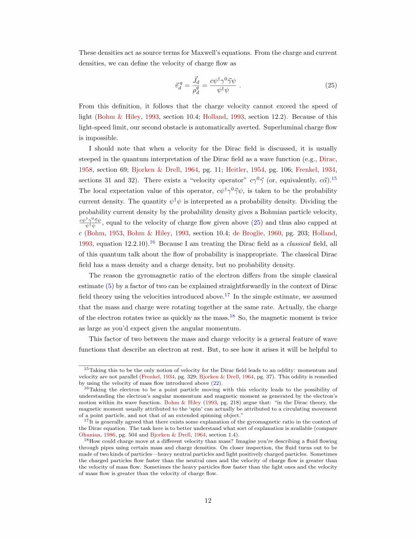
These densities act as source terms for Maxwell’s equations. From the charge and current

densities, we can define the velocity of charge flow as

~v qd =~Jdρqd

=cψ†γ0~γψ

ψ†ψ. (25)

From this definition, it follows that the charge velocity cannot exceed the speed of

light (Bohm & Hiley, 1993, section 10.4; Holland, 1993, section 12.2). Because of this

light-speed limit, our second obstacle is automatically averted. Superluminal charge flow

is impossible.

I should note that when a velocity for the Dirac field is discussed, it is usually

steeped in the quantum interpretation of the Dirac field as a wave function (e.g., Dirac,

1958, section 69; Bjorken & Drell, 1964, pg. 11; Heitler, 1954, pg. 106; Frenkel, 1934,

sections 31 and 32). There exists a “velocity operator” cγ0~γ (or, equivalently, c~α).15

The local expectation value of this operator, cψ†γ0~γψ, is taken to be the probability

current density. The quantity ψ†ψ is interpreted as a probability density. Dividing the

probability current density by the probability density gives a Bohmian particle velocity,cψ†γ0~γψψ†ψ

, equal to the velocity of charge flow given above (25) and thus also capped at

c (Bohm, 1953, Bohm & Hiley, 1993, section 10.4; de Broglie, 1960, pg. 203; Holland,

1993, equation 12.2.10).16 Because I am treating the Dirac field as a classical field, all

of this quantum talk about the flow of probability is inappropriate. The classical Dirac

field has a mass density and a charge density, but no probability density.

The reason the gyromagnetic ratio of the electron differs from the simple classical

estimate (5) by a factor of two can be explained straightforwardly in the context of Dirac

field theory using the velocities introduced above.17 In the simple estimate, we assumed

that the mass and charge were rotating together at the same rate. Actually, the charge

of the electron rotates twice as quickly as the mass.18 So, the magnetic moment is twice

as large as you’d expect given the angular momentum.

This factor of two between the mass and charge velocity is a general feature of wave

functions that describe an electron at rest. But, to see how it arises it will be helpful to

15Taking this to be the only notion of velocity for the Dirac field leads to an oddity: momentum andvelocity are not parallel (Frenkel, 1934, pg. 329; Bjorken & Drell, 1964, pg. 37). This oddity is remediedby using the velocity of mass flow introduced above (22).

16Taking the electron to be a point particle moving with this velocity leads to the possibility ofunderstanding the electron’s angular momentum and magnetic moment as generated by the electron’smotion within its wave function. Bohm & Hiley (1993, pg. 218) argue that: “in the Dirac theory, themagnetic moment usually attributed to the ‘spin’ can actually be attributed to a circulating movementof a point particle, and not that of an extended spinning object.”

17It is generally agreed that there exists some explanation of the gyromagnetic ratio in the context ofthe Dirac equation. The task here is to better understand what sort of explanation is available (compareOhanian, 1986, pg. 504 and Bjorken & Drell, 1964, section 1.4).

18How could charge move at a different velocity than mass? Imagine you’re describing a fluid flowingthrough pipes using certain mass and charge densities. On closer inspection, the fluid turns out to bemade of two kinds of particles—heavy neutral particles and light positively charged particles. Sometimesthe charged particles flow faster than the neutral ones and the velocity of charge flow is greater thanthe velocity of mass flow. Sometimes the heavy particles flow faster than the light ones and the velocityof mass flow is greater than the velocity of charge flow.

12

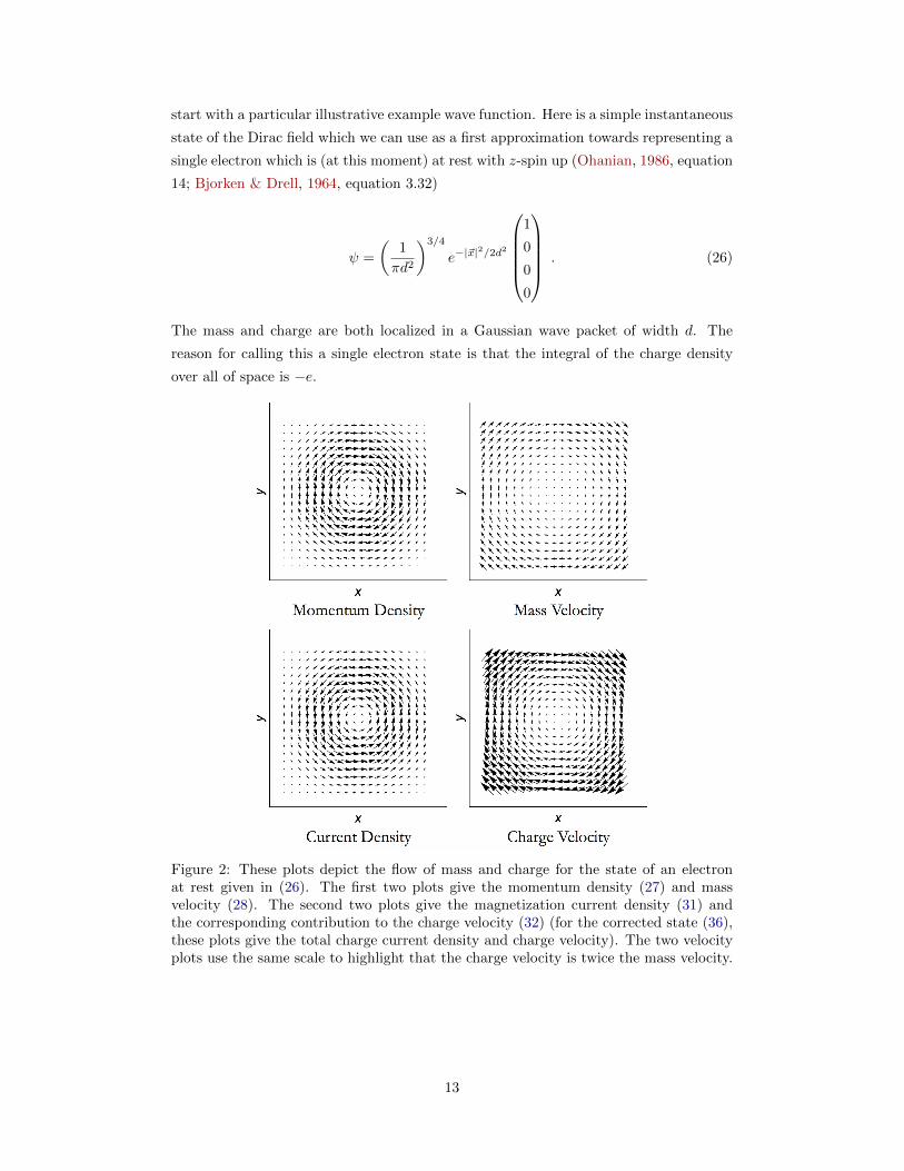
start with a particular illustrative example wave function. Here is a simple instantaneous

state of the Dirac field which we can use as a first approximation towards representing a

single electron which is (at this moment) at rest with z-spin up (Ohanian, 1986, equation

14; Bjorken & Drell, 1964, equation 3.32)

ψ =

(1

πd2

)3/4

e−|~x|2/2d2

1

0

0

0

. (26)

The mass and charge are both localized in a Gaussian wave packet of width d. The

reason for calling this a single electron state is that the integral of the charge density

over all of space is −e.

Figure 2: These plots depict the flow of mass and charge for the state of an electronat rest given in (26). The first two plots give the momentum density (27) and massvelocity (28). The second two plots give the magnetization current density (31) andthe corresponding contribution to the charge velocity (32) (for the corrected state (36),these plots give the total charge current density and charge velocity). The two velocityplots use the same scale to highlight that the charge velocity is twice the mass velocity.

13

The momentum density for this state is

~Gd =~2

(1

πd2

)3/2

e−|~x|2/d2 ~x× z

d2, (27)

calculated via (19) where only the second term is non-zero. From this expression, it

is clear that mass and energy are flowing around the z-axis (see figure 2). The mass

velocity for this state can be calculated by dividing this momentum density by the mass

density as in (22),

~vd =~

2m

~x× zd2

=~r

2md2θ . (28)

The second expression gives the velocity in cylindrical coordinates. This equation shows

that the mass flows everywhere about the z-axis at constant angular velocity. The

electron’s mass appears19 to rotate like a solid object.

To calculate the velocity at which charge flows, it is useful to first expand the current

density using the free Dirac equation as follows20

− ecψ†γ0~γψ =ie~2m

{ψ†γ0~∇ψ − (~∇ψ†)γ0ψ

}︸ ︷︷ ︸

¬

− e~2m

~∇× (ψ†γ0~σψ)︸ ︷︷ ︸­

+ie~2mc

∂

∂t(ψ†~γψ)︸ ︷︷ ︸

®

.

(29)

The three terms in the expansion are the convection current density, the magnetization

current density, and the polarization current density. As was the case for the momentum

density (19), the first term is zero for an electron at rest. The second two terms give

the contribution to the charge current from spin. For the moment, let us focus on the

magnetization current density. The magnetization current density in (29) corresponds

to a magnetic moment density of

− e~2mc

ψ†γ0~σψ , (30)

where the prefactor is the Bohr magneton.21 The ratio of the magnitude of this magnetic

moment density to the magnitude of the angular moment density in (20) for the state

in (26) is emc , the correct gyromagnetic ratio for the electron (6). The magnetization

current density,

−e~2mc

(1

πd2

)3/2

e−|~x|2/d2 ~x× z

d2, (31)

makes a contribution to the velocity of charge flow, calculated via (25), of

~m

~x× zd2

=~rmd2

θ . (32)

19I use the qualification “appears” because, as will be explained shortly, (26) is not an entirelysatisfactory approximation to the state of an electron.

20This expansion appears in Frenkel (1934, pg. 321–322); Ohanian (1986, pg. 504).21See Jackson (1999, section 5.6); Ohanian (1986, pg. 504).

14

The contribution to the velocity of charge flow which determines the electron’s magnetic

moment (32) is twice the velocity of mass flow which determines the electron’s angular

momentum (28).

The factor of two between these velocities is not a peculiar feature of the chosen

state, but will hold for any electron state in the non-relativistic limit. In general, the

contribution to the moment density ~Gd from spin is ~4~∇ × (ψ†~σψ)—the second term

in (19). In the non-relativistic limit, the relativistic mass density is approximately

mψ†γ0ψ—the first term in (21). Dividing these, as in (22), gives a contribution to the

velocity of mass flow from spin of

~4m

~∇× (ψ†~σψ)

ψ†γ0ψ. (33)

The velocity associated with the electron’s spin magnetic moment can be derived from

the magnetization current density—the second term in (29). Dividing the magnetization

current density by the charge density (23) as in (25) yields a contribution to the charge

velocity of

~2m

~∇× (ψ†γ0~σψ)

ψ†ψ. (34)

It is clear that (34) is twice (33) (up to factors of γ0 which we will return to later).

Addressing our obstacles in the context of the Dirac equation has enabled significant

progress, but there remain three serious shortcomings to the account given thus far

which will be resolved in the following section. First, we have only been able to say

(somewhat awkwardly) that a certain contribution to the velocity of charge flow is twice

the velocity of mass flow and not that the actual velocity of charge flow is twice the

velocity of mass flow. In fact, it is easy to see that the velocity of charge flow is zero

for the state in (26) as the charge current density calculated from (24) is clearly zero.

The first term in the current expansion (29) is also zero. Thus, one can see that the

third term in (29) (the polarization current density) will exactly cancel the second (the

magnetization current density). Because of this cancellation, no magnetic field is being

produced by an electron in this state. If we are to account for the magnetic field around

an electron at rest, the electron’s charge must actually rotate.

Second, the velocities in (28) and (32) are unbounded, becoming superluminal as r

becomes very large. The fact that (32) becomes infinite is less troubling because, as

was just discussed, it is cancelled by the contribution to the charge velocity from the

polarization current. Also, as was mentioned earlier, it can be shown in general that

the charge velocity cannot exceed c. The fact that (28) becomes superluminal is a real

problem.

Third, there are problems which arise if the electron is too small and as of yet we

have no reason to think it’s large enough to avoid these problems. If the electron is

too small, we face our first two obstacles concerning superluminal rotation. Also, if the

electron is too small we will not be able to ignore the mass in the electromagnetic field

15

when calculating the gyromagnetic ratio (as was done in this section but not the last).

Looking at (26) it appears that the size of the electron is an entirely contingent matter

depending on the state of the Dirac field. By decreasing d, the electron can be made

arbitrarily small.

5 The Dirac Sea

The three problems raised at the end of the previous section can be resolved by restricting

the allowed states of the Dirac field to those formed by superposing positive frequency

modes. Such a restriction can be motivated as a way of implementing the idea of a Dirac

sea in the context of classical Dirac field theory, though this move does not involve the

postulation of an infinite sea of electrons.

In this section we will continue to restrict our attention to the free Dirac

equation, putting aside issues of self-interaction—the electron is treated as blind to

the electromagnetic field it generates—but still confronting issues of self-energy—the

energies of the Dirac and electromagnetic fields are both taken into account in the

following analysis.

The free Dirac equation admits of plane wave solutions with definite22 momentum

~p and time dependence given by either e−iEt/~ (positive frequency) or eiEt/~ (negative

frequency), where E is the energy associated with that momentum, E =√|~p|2c2 +m2c4

(Bjorken & Drell, 1964, chapter 3). From (18), it is clear that the positive frequency

plane waves have uniform positive energy density and the negative frequency plane waves

have uniform negative energy density.

On a quantum interpretation of the Dirac field, one would say that these plane wave

solutions are eigenstates of momentum and energy where the energy eigenvalues may be

positive or negative. The existence of such negative energy states proved both a blessing

and a curse for early applications of the Dirac equation. To retain the blessing while

dispelling the curse, Dirac proposed his hole theory according to which all of the negative

energy states are filled (Dirac, 1930). By Pauli exclusion, any additional electrons must

sit atop this “Dirac sea.” The filled sea is taken to set the zero level for energy and

charge. If any electron is excited out of the sea, the hole it leaves behind acts like a

particle with equal mass and opposite charge to the electron—a positron. The possibility

of creating such holes in the Dirac sea is essential for understanding many phenomena

(including vacuum polarization, which would be important in a more thorough analysis

of the Dirac and electromagnetic fields of an electron at rest). However, the discussion

here will be simplified by assuming the Dirac sea to be filled. It is this rise in sea level,

not the presence of holes, which is the key to solving our remaining problems.

Although the Dirac sea is generally explained in these quantum mechanical terms,

22On a classical interpretation of the Dirac field, by saying the momentum is “definite” I mean thatthe momentum density (19) is uniform.

16

the simplified version of it described above—where the sea is always filled—can be easily

implemented in the context of the classical interpretation of the Dirac equation where

the Dirac field is viewed as a classical field. The change that must be made to classical

Dirac field theory as presented in the previous section is not any change to the dynamical

laws, but simply a shrinking of the space of possible states. Any state of the Dirac field

which has a Fourier decomposition that includes negative frequency modes is forbidden.

All allowed physical states are to be formed entirely from positive energy modes. Let us

call this theory “restricted Dirac field theory.” Restricted Dirac field theory incorporates

important features of the Dirac sea without positing an infinite sea of electrons pervading

all of space.

A different modification to classical Dirac field theory would be necessary to fully

implement the idea of the Dirac sea (including the possibility of holes) and would

certainly be required if we were considering interactions that could take states composed

only of positive frequency modes into states containing both positive and negative

frequency modes. This is a topic I hope to examine in future work. I expect that

in such a theory both positive and negative frequency modes would be allowed, but the

equation for charge density (23) would be revised so that negative frequency modes carry

positive charge (as these modes would be associated with positrons). To keep things

relatively simple, we will not consider such a full implementation of the Dirac sea here.

We will focus on restricted Dirac field theory.

As was first examined by Weisskopf (1934a,b, 1939), the electromagnetic energy

divergence—which arises because the amount of energy in an electron’s electromagnetic

field goes rapidly to infinity as its radius is decreased—is tamed in the context of hole

theory (Schweber, 1994, section 2.5.3). Weisskopf’s handling of this divergence in hole

theory has been incorporated into the modern understanding of mass renormalization

within quantum electrodynamics.23 The crucial insight from Weisskopf’s analysis for

our task at hand is expressed well by Heitler (1954, pg. 299). He writes that the taming

of the electromagnetic self-energy divergence for an electron at rest “is a consequence of

the hole theory and the Pauli [exclusion] principle”:

“Consider an electron represented by a very small wave packet in coordinate

space. In momentum space this would be represented by a distribution

including negative energy states. The latter, however, are filled with vacuum

electrons. Consequently, the negative energy contributions to the wave

function must be eliminated and the electron cannot be a wave packet of

infinitely small size but must have a finite extension (of the order ~mc [the

Compton radius], as one easily finds). Consequently the static self-energy

will be diminished also.”

This explanation is given from within the quantum interpretation of the Dirac field as

23It is cited in relation to the Feynman diagram approach by Schweber (1961, pg. 513); Bjorken &Drell (1964, pg. 165); Gottfried & Weisskopf (1986, section II.D.2).

17

wave function. But, it contains lessons that carry over to the classical interpretation:

There is a limit on the minimum size wave packet that one can construct from the

positive frequency modes of the Dirac field that are available in restricted Dirac field

theory. The mass and charge of the electron cannot be confined to an arbitrarily small

volume.24 Because the charge of the electron is spread over such a large packet, the

electromagnetic contribution to the energy (and mass) of an electron at rest is small

and can be ignored when calculating the gyromagnetic ratio to a first approximation

(as was done in the previous section). In section 2 we saw that in order to avoid the

superluminal rotation speeds forced upon us in our first two obstacles, the electron must

be at least as large as the Compton radius. The classical implementation of the Dirac

sea delivers that minimum size.

Let us return to the instantaneous electron state in (26). In restricted Dirac field

theory, this state is forbidden as it includes both positive and negative frequency modes.

To find a similar state that is allowed, we can simply delete the negative frequency

modes from the Fourier decomposition of (26).25 This yields26

ψ =1

2

(d2

π~2

)3/4(1

2π~

)3/2 ˆd3p

(1 +

mc2

E

)e−

|~p|2d2

2~2 + i~ ~p·~x

1

0pzc

E+mc2

(px+ipy)cE+mc2

. (35)

We can approximate this state in the non-relativistic limit by computing these integrals

assuming that d � ~mc so the momentum space Gaussian in the integrand suppresses

modes where |~p|2 is not � m2c2,27

ψ =

(1

πd2

)3/4

e−|~x|2/2d2

1

0~

2mcd2 iz

~2mcd2 (ix− y)

. (36)

The total current density for this state (36), calculated via (24), is equal to the

previous magnetization current density (31). Dividing this by the charge density for

24Although we have not discussed in detail the above-mentioned deeper modification of classical Diracfield theory needed to fully implement the idea of the Dirac sea (including holes), it is hard to see howthat theory would allow for the electron’s charge to be confined to a smaller volume. Holding fixed thatthe total charge in the Dirac field is −e, the presence of negative energy modes with positive chargedensity will only make it harder to localize the electron’s charge in a small region.

25This Fourier decomposition is given in Bjorken & Drell, 1964, section 3.3.26As the negative frequency modes have simply been deleted, this new state is not normalized. In

our classical terms, this means that the integral of the charge density over all space will not be −e. Inthe non-relativistic limit, the total charge will be close to −e.

27The same approximation can be arrived at by trusting only the first two components of (26) andusing the positive frequency non-relativistic limit of the Dirac equation in Bjorken & Drell (1964, eq.1.31) to calculate the other two.

18

(36) gives a charge velocity of

~v qd =~

md2 ~x× z1 + ~2

m2c2d4 |~x|2. (37)

This limits to (32) for d � ~mc . Unlike (32), this is the actual charge velocity and not

merely a contribution to it. The charge is really moving. The velocity in (37) is bounded

and will not exceed the speed of light—as must be the case since the definition of the

charge velocity (25) ensures that it cannot be superluminal. For d � ~mc , the mass

velocity derived from (36) using (22) will be as it was before (28). Thus, the charge

rotates twice as fast as the mass.

This factor of two between mass and charge velocity is a general feature of states

that describe electrons at rest in restricted Dirac field theory. What prevented us from

reaching this conclusion in the previous section was that we had no reason to suppose the

magnetization current density would be the dominant contribution to the total current

density (29). The polarization current density could be significant as well. By restricting

ourselves to superpositions of positive frequency modes, we have guaranteed that the

polarization current density is small. To see why this is so, consider an arbitrary state

of the Dirac field at an arbitrary time labeled t = 0, ψ(0). This state can be written

as the sum of a superposition of positive frequency modes, ψ+, and a superposition of

negative frequency modes, ψ−. In the non-relativistic limit, the time dependence of this

state is given by

ψ(t) = e(imc2/~)tψ+ + e−(imc

2/~)tψ− . (38)

The polarization current density for this state is

ie~2mc

∂

∂t

(ψ†+~γψ+ + e−2(imc

2/~)tψ†+~γψ− + e2(imc2/~)tψ†−~γψ+ + ψ†−~γψ−

). (39)

If we forbid negative frequency modes, the cross terms are absent and the time derivative

yields zero. Thus, in the non-relativistic limit the polarization current density is

negligible.

In the previous section we were able to derive the factor of two between charge

velocity and mass velocity only up to factors of γ0. The reason these factors can be

ignored is that γ0 simply flips the sign of the third and fourth components of ψ and these

components—for a state composed of positive frequency modes in the non-relativistic

limit—are much smaller than the first and second components.

At this point let us reflect on the role that the non-relativistic limit has played in

the preceding analysis. This limit is not part of the general response to our first two

obstacles. The fact that there is a minimum size for wave packets formed from positive

frequency modes is not dependent on this limit, nor is the light-speed cap on charge

velocity. The non-relativistic limit is, however, essential in explaining the electron’s

gyromagnetic ratio. The reason for this is that the gyromagnetic ratio we seek to account

19

for only holds in the non-relativistic limit.28 Beyond this limit, the relationship between

angular momentum and magnetic moment is more complex. In quantum mechanical

terms, the relationship is given by the claim that the spin magnetic moment operator,

− e~2mcγ

0~σ, is − eγ0

mc times the spin angular momentum operator, ~2~σ (Ohanian, 1986, pg.

504; Frenkel, 1934, pg. 323). Expressed in terms of local expectation values, the local

ratio of spin magnetic momentum to angular momentum is the ratio of − e~2mcψ

†γ0~σψ

to ~2ψ†~σψ. In our classical field terminology, this is understood as the ratio of the spin

magnetic moment density (30) to the spin angular momentum density (20).

6 Conclusion

The consensus about electron spin, which emerged long ago, is that the electron somehow

acts like a spinning object without actually spinning. As Rojansky (1938, pg. 514) puts

it in his textbook on quantum mechanics, after discussing spin angular momentum and

spin magnetic moment in the context of the Dirac equation,

“In short, Dirac’s equation automatically endows the electron with the

properties that account for the phenomena previously ascribed to a

hypothetical spinning motion of the electron.” (original italics)

Here I have argued for a different interpretation. The Dirac equation does not somehow

manage to account for these properties without positing a spinning electron. Instead, it

explains just how the electron spins.

The obstacles to regarding the electron as spinning presented in the introduction

were addressed as follows: Old estimates of the size of the electron made under

the assumption that the electron’s mass is primarily electromagnetic suggest that

the electron would have to rotate superluminally in order to have the right angular

momentum and magnetic moment. Actually, if the electron’s mass is primarily

electromagnetic we should focus on the rotation of the electromagnetic field’s mass in

calculating the electron’s angular momentum and this mass cannot move superluminally.

Also, the electron’s mass is not primarily electromagnetic. When we move to better

estimates of the electron’s size—using the Dirac field to represent the state of the

electron—we see that its minimum size is large enough that there is no need for

superluminal rotation. Further, the definition of charge velocity for the Dirac field

guarantees that the electron’s charge will not move superluminally. The other obstacle

was the fact that the electron’s gyromagnetic ratio differs from the simplest classical

estimate by a factor of two. On the account given here, this factor does not arise

from some novel quantum revision to the basic physical principles defining angular

momentum and magnetic moment, but is instead attributed to a false assumption in

the simple classical estimate—the electron’s mass and charge do not rotate at the same

28Standard explanations of the factor of two in the gyromagnetic ratio of the electron using the Diracequation appeal to the non-relativistic limit (Bjorken & Drell, 1964, section 1.4).

20

rate.

Acknowledgments Thank you to Adam Becker, Dirk-Andre Deckert, John

McGreevy, Lukas Nickel, Hans Ohanian, Laura Ruetsche, Roderich Tumulka, David

Wallace, and anonymous referees for helpful feedback and discussion. This project

was supported in part by funding from the President’s Research Fellowships in the

Humanities, University of California.

References

Barut, A.O. 1988. Quantum-electrodynamics based on self-energy. Physica Scripta,

1988(T21), 18–21.

Barut, A.O., & Dowling, Jonathan P. 1990. Self-field quantum electrodynamics: The

two-level atom. Physical Review A, 41(5), 2284–2294.

Bialynicki-Birula, Iwo. 1996. The photon wave function. Pages 313–322 of: Eberly,

Joseph H., Mandel, Leonard, & Wolf, Emil (eds), Coherence and Quantum Optics

VII: Proceedings of the Seventh Rochester Conference on Coherence and Quantum

Optics, held at the University of Rochester, June 7–10, 1995. Springer. An extended

version of this article is available at http://arxiv.org/abs/quant-ph/0508202.

Bjorken, James D., & Drell, Sydney D. 1964. Relativistic Quantum Mechanics.

McGraw-Hill.

Bohm, David. 1953. Comments on an article of Takabayasi concerning the formulation

of quantum mechanics with classical pictures. Progress of Theoretical Physics, 9(3),

273–287.

Bohm, David, & Hiley, Basil J. 1993. The Undivided Universe: An ontological

interpretation of quantum theory. Routledge.

Carroll, Sean M. 2016. You should love (or at least respect) the Schrodinger equation.

[Online; accessed 17-August-2017]

http://www.preposterousuniverse.com/blog/2016/08/15/

you-should-love-or-at-least-respect-the-schrodinger-equation/.

Colin, Samuel. 2004. Beables for quantum electrodynamics. Annales de la Fondation

Louis de Broglie, 29(1–2), 273–296.

Corben, H.C. 1961. Spin in classical and quantum theory. Physical Review, 121(6),

1833–1839.

Crisp, Michael Dennis, & Jaynes, E.T. 1969. Radiative effects in semiclassical theory.

Physical Review, 179(5), 1253–1261.

21

de Broglie, Louis. 1960. Non-Linear Wave Mechanics: A causal interpretation. Elsevier.

Dirac, Paul A.M. 1930. A theory of electrons and protons. Proceedings of the Royal

Society of London A: Mathematical, Physical and Engineering Sciences, 126(801),

360–365.

Dirac, Paul A.M. 1958. The Principles of Quantum Mechanics. 4 edn. Oxford University

Press.

Duncan, Anthony. 2012. The Conceptual Framework of Quantum Field Theory. Oxford

University Press.

Durr, Detlef, Goldstein, Sheldon, Tumulka, Roderich, & Zanghı, Nino. 2005. Bell-type

quantum field theories. Journal of Physics A: Mathematical and General, 38(4),

R1–R43.

Einstein, Albert. 1906. The principle of conservation of motion of the center of gravity

and the inertia of energy. Annalen der Physik, 20, 627–633.

Feynman, Richard P., Leighton, Robert B., & Sands, Matthew. 1964. The Feynman

Lectures on Physics. Vol. II. Addison-Wesley Publishing Company.

Frenkel, J. 1934. Wave Mechanics: Advanced General Theory. Oxford University Press.

Giulini, Domenico. 2008. Electron spin or “classically non-describable two-valuedness”.

Studies In History and Philosophy of Science Part B: Studies In History and

Philosophy of Modern Physics, 39(3), 557–578.

Good, Roland H., Jr. 1957. Particle aspect of the electromagnetic field equations.

Physical Review, 105(6), 1914–1919.

Gottfried, Kurt, & Weisskopf, Victor F. 1986. Concepts of Particle Physics. Vol. 2.

Oxford University Press.

Goudsmit, Samuel A. 1998. The discovery of electron spin. Chap. 1, pages 2–12 of:

Gareth R. Eaton, Sandra S. Eaton, Kev M. Salikhov (ed), Foundations Of Modern

EPR. World Scientific.

Griffiths, David J. 1999. Introduction to Electrodynamics. 3 edn. Prentice Hall.

Griffiths, David J. 2005. Introduction to Quantum Mechanics. 2 edn. Pearson Prentice

Hall.

Hatfield, Brian. 1992. Quantum Theory of Point Particles and Strings. Addison-Wesley.

Frontiers in Physics, Volume 75.

Heitler, Walter H. 1954. The Quantum Theory of Radiation. 3 edn. Oxford University

Press.

Holland, Peter R. 1993. The Quantum Theory of Motion: An account of the de

Broglie-Bohm causal interpretation of quantum mechanics. Cambridge University

22

Press.

Jackson, John D. 1999. Classical Electrodynamics. 3 edn. Wiley.

Jaynes, E.T. 1973. Survey of the present status of neoclassical radiation theory. Pages

35–81 of: Mandel, L., & Wolf, E. (eds), Coherence and Quantum Optics. Plenum

Press.

Lange, Marc. 2002. An Introduction to the Philosophy of Physics: Locality, Energy,

Fields, and Mass. Blackwell.

MacGregor, Malcolm H. 1992. The Enigmatic Electron. Kluwer Academic Publishers.

Mignani, E, Recami, E, & Baldo, M. 1974. About a Dirac-like equation for the

photon according to Ettore Majorana. Lettere al Nuovo Cimento (1971-1985), 11(12),

568–572.

Ohanian, Hans C. 1986. What is spin? American Journal of Physics, 54(6), 500–505.

Pais, Abraham. 1989. George Uhlenbeck and the discovery of electron spin. Physics

Today, 42(12), 34–40.

Pashby, Thomas. 2012. Dirac’s prediction of the positron: a case study for the current

realism debate. Perspectives on Science, 20(4), 440–475.

Pauli, Wolfgang. 1980. General Principles of Quantum Mechanics. Springer-Verlag.

Pearle, Philip. 1982. Classical electron models. Pages 211–295 of: Teplitz, Doris (ed),

Electromagnetism: Paths to Research. Plenum Press.

Peskin, Michael E., & Schroeder, Daniel V. 1995. An Introduction to Quantum Field

Theory. Westview Press.

Poincare, Henri. 1900. La theorie de Lorentz et le principe de reaction. Archives

neerlandaises des sciences exactes et naturelles, 5, 252–278. Translation by S.

Lawrence 2008 at http://www.physicsinsights.org/poincare-1900.pdf.

Rohrlich, Fritz. 2007. Classical Charged Particles. 3 edn. World Scientific.

Rojansky, Vladimir. 1938. Introductory Quantum Mechanics. Prentice-Hall.

Schweber, Silvan S. 1961. Introduction to Relativistic Quantum Field Theory. Harper &

Row.

Schweber, Silvan S. 1994. QED and the Men Who Made It: Dyson, Heynman,

Schwinger, and Tomanaga. Princeton University Press.

Sebens, Charles T. forthcoming. Forces on fields. Studies in History and Philosophy of

Modern Physics.

Struyve, Ward. 2010. Pilot-wave theory and quantum fields. Reports on Progress in

Physics, 73(10), 106001.

23

Teller, Paul. 1995. An interpretive introduction to quantum field theory. Princeton

University Press.

Tomonaga, Sin-itiro. 1997. The Story of Spin. University of Chicago Press.

Tong, David. 2006. Lectures on Quantum Field Theory. http://www.damtp.cam.ac.

uk/user/tong/qft.html [Online; accessed 2-August-2017].

Uhlenbeck, George E. 1976. Fifty years of spin: Personal reminiscences. Physics Today,

29(6), 43–48.

Valentini, Antony. 1992. On the pilot-wave theory of classical, quantum and subquantum

physics. Ph.D. thesis, ISAS, Trieste, Italy.

Valentini, Antony. 1996. Pilot-wave theory of fields, gravitation, and cosmology. Pages

45–66 of: Cushing, James T., Fine, Arthur, & Goldstein, Sheldon (eds), Bohmian

Mechanics and Quantum Theory: An Appraisal. Kluwer Academic.

Wallace, David. forthcoming. The quantum theory of fields. In: Knox, Eleanor, &

Wilson, Alastair (eds), Handbook of Philosophy of Physics.

Weinberg, Steven. 1999. What is quantum field theory, and what did we think it was?

Pages 241–251 of: Cao, Tian Yu (ed), Conceptual Foundations of Quantum Field

Theory. Cambridge University Press.

Weisskopf, V. 1934a. Uber die selbstenergie des elektrons. Zeitschrift fur Physik, 89,

27–39.

Weisskopf, V. 1934b. Berichtigung zu der arbeit: uber die selbstenergie des elektrons.

Zeitschrift fur Physik, 90, 817–818.

Weisskopf, Victor F. 1939. On the self-energy and the electromagnetic field of the

electron. Physical Review, 56(1), 72–85.

Wentzel, Gregor. 1949. Quantum Theory of Fields. Interscience Publishers.

Weyl, Hermann. 1932. The Theory of Groups and Quantum Mechanics. Dover.

24