How do political dynasties affect economic development?

Theory and Evidence from India∗

Siddharth Eapen George & Dominic Ponattu

May 26, 2018

Abstract

Political dynasties are present in more than 144 countries, yet we have ambiguous theoretical predictions

and limited empirical evidence about the economic impacts of dynastic rule. Bequest motives may encourage

dynasts to make investments that regular politicians would not; but inheriting political capital could weaken

the selection and incentives of dynastic descendants. We compile data on the family connections of over 105,000

Indian politicians, and document high levels of dynasticism and low intergenerational mobility in Indian poli-

tics. We estimate the causal effect of dynastic rule using a close elections RD design that compares constituen-

cies where dynasts narrowly win to constituencies where dynasts narrowly lose. We find that dynastic rule

negatively impacts local economic development: dynast-ruled areas have 0.2 std dev slower night-time lights

growth, worse public good provision, and voters assess dynastic MPs to perform worse. Close family are the

worst-performing dynasts, but our results are not driven by a left tail of “lemon dynasts”; rather, dynasts under-

perform along the whole performance distribution. Dynastic politicians appear to have lower electoral returns

from good in-office performance, suggesting that inherited electoral advantages may mute incentives. A com-

parison with celebrity politicians suggests that name recognition cannot be ruled out as the source of dynasts’

electoral advantage. Politicians with sons perform better in-office, suggesting that incentives to establish a dy-

nasty can motivate better performance.

∗Siddharth Eapen George, siddharthgeorge@fas.harvard.edu, Harvard University, Cambridge, MA, USA; Dominic Ponattu,dponattu@mail.uni-mannheim.de, University of Mannheim, Germany. We thank Sreevidya Gowda for research assistance.We are grateful to Alberto Alesina, Abhijit Banerjee, Robert Bates, Kirill Borusyak, Emily Breza, Felipe Campante, MelissaDell, Max Gopelrud, Asim Khwaja, Michael Kremer, Nathan Nunn, Rohini Pande, Pia Raffler, Daniel Smith, Andrei Shleifer,Henrik Sigstad, Edoardo Teso and Chenzi Xu for helpful conversations. We thank participants at the Midwest Political ScienceAssociation Conference 2016, the Northeast Universities Development Conference 2017, the MIT Political Economy lunch andHarvard’s development, political economy and comparative politics seminars and Mannheim’s political economy seminarsfor ideas and useful feedback. Financial support from the Lab for Economic Applications and Policy and the Warburg Fund isacknowledged.

1

1 Introduction

Political dynasties are present in over 144 countries around the world and are a frequent topic of

public discussion. Yet we have ambiguous theoretical predictions and limited empirical evidence

about how dynastic rule affects economic development. This paper attempts to: (i) provide well-

identified evidence on the local economic impacts of dynastic rule, (ii) understand the mechanisms

that drive these effects and (iii) suggest a theory for why dynasties may underperform but persist.

A key difference between dynastic and non-dynastic politicians is that dynasts receive and bequest

political capital across generations. These transfers affect the selection and incentives—–and therefore

the performance—–of dynastic politicians. Bequest motives may cause dynasts to have a longer time

horizon and enable them to make investments that regular, electoral cycle-bound politicians will not.

Dynasts may in this sense be the political analog of family firms (Burkart, Panunzi and Shleifer 2003).

One the other hand, inheriting political capital — a prominent name, a positive reputation, a

powerful network, a party machine — may give dynastic descendants electoral advantages (Smith

2012) and may worsen governance because of adverse selection (by encouraging “lemon dynasts”

to seek office) and moral hazard (by dampening the performance incentives of incumbent dynasts).

Potential challengers may be deterred, believing that dynasts are hard to beat, so dynastic rule may

also have a chilling effect on political competition.

We compile novel data on the family connections of every candidate contesting state and national

assembly elections in India from 2003. We document that dynasties are both prevalent and persistent

in Indian politics: 3.9% of candidates and 10% of winners are children of former politicians. Moreover,

intergenerational mobility in politics is low: the father-child vote share correlation is 0.84, implying

that a non-trivial portion of political capital appears heritable.

To estimate the effects of dynastic rule, we use a close elections RD design. We focus on races

between dynasts and non-dynasts, and compare constituencies where a dynast narrowly won to those

where a dynast narrowly lost. Our main baseline result is that dynastic rule negatively impacts local

economic development in the short run. Dynast-ruled constituencies experience 6.5pp (~0.2 std dev)

slower night-time lights growth during the term in office, and this result is robust to comparing

2

border villages in the same administrative district but different political constituencies. Public good

provision also worsens (~0.14 std dev) and dynasts are rated by voters to perform worse (~0.28 std

dev).

Why do dynasts underperform and why are they so over-represented in political equilibrium?

First, we argue that our results are unlikely to be driven by a left-tail of “lemon” dynastic winners in

marginal races. Dynasts and non-dynasts in close races appear relatively similar on observable char-

acteristics. Moreover, non-dynasts outperform dynasts at all points of the performance distribution,

suggesting that as a group they face different selection or incentives.

Second, we find that close family—–sons, daughter and wives—–are the worst performing dy-

nasts. This finding mirrors the family firms literature and suggests that lower barriers to entry for

these candidates may explain dynastic underperformance. Third, we find that dynastic politicians

appear to have advantages in organising clientelistic transfers, particularly within their ethnic group.

They are more likely to buy votes from co-ethnics despite voters reporting that they spend less in

elections.

We compare dynasts to celebrity politicians—–film stars and cricketers—–and cannot reject that

dynasts’ electoral advantages come from name recognition. We also do not find that dynastic victory

at election t reduces political competition in subsequent elections or that dynast are more likely to

rent-seek while in office.

Finally, we show that politicians with sons perform better in-office than those without sons. In

the context of India, where women face severe barriers to entering politics, incumbents without sons

may not have heirs, we interpret this as evidence that bequest motives can incentivise better in-office

performance.

Our argument and findings relate to a small bur growing literature on political dynasties, sum-

marised recently by Geys and Smith (2017). This literature has mostly focused on documenting that

power begets power ie. that dynasties arise and persist due to factors other than familial variation

in political acumen (Smith 2012; Querubin 2015, 2013). Dal Bó, Dal Bó and Snyder (2009) show that

holding legislative office in the US House increases the probability that family members subsequently

enter the House. Querubin (2015) and Rossi (2014) also find that holding legislative office raises the

3

probability that one’s relatives do, in the Philippines and Argentina respectively. Querubin (2013)

shows that institutional measures like term limits which do not tackle the underlying source of dynas-

tic power can be quite ineffective at reducing persistence. Fiva and Smith (2018) show that intra-party

networks may explain dynastic persistence, and Smith (2018) demonstrates that electoral rules and

party structure significantly influence where dynasties arise and persist. Tantri and Thota (2017) also

study the performance of dynastic politicians in India, and find that marginal dynasts underperform

relative to regular politicians.

The remainder of the paper is organised as follows. Section 2 contains background on political

dynasties in India. Section 3 describes the data used. Section 4 outlines the empirical strategy. Section

5 presents baseline results. Section 6 shows robustness checks. Section 7 discusses – and tests –

candidate mechanisms, and Section 8 concludes.

2 Background

India has a federal political structure, with national, state and local assemblies. While political dy-

nasties are likely to exist at all levels, we focus in this paper on members of the Lok Sabha (Lower

House), India’s national parliament. There are 543 MPs, whose role involves a mixture of legislative

and constituency obligations. Each MP is elected from a single-member electoral district via plural-

ity rule. Each term lasts 5 years (or until the Lok Sabha is dissolved) and there is no term limit. The

Nehru-Gandhi family, which leads the Indian National Congress, the party that won India’s indepen-

dence, is perhaps the most well-known political dynasty but there are other less well-known political

families, including the Sinha family (father and son Finance Ministers), the Pilot family (father and

son Union Ministers) and the Gogoi family (Chief Minister of Assam and MP).

4

3 Data

3.1 Family connections

We compile data on the family connections of all candidates in state and national parliament elections

from 2003. We digitise, scrape, clean and merge over 105,000 nomination papers in order to compile

dynastic connections for the universe of Indian politicians in national and state assembly elections

from 2003. We verify this procedure of identify dynastic links by conducting biographical research

on winners and runners-up in close races to the Lok Sabha from 1999-2014 and combining with data

from the work of Patrick French (2011).

We first document the prevalence and persistence of dynasties in Indian politics. 1 and 2 show that

on average nearly 4% of candidates and 10% of winners are dynasts. This average figure masks sub-

stantial variation across states from 12% of candidates being dynastic in Punjab to just 2.1% in Tamil

Nadu. Contrary to popular perception, there are fewer differences across parties in the fraction of

dynastic candidates. Both the Congress party (predictably) and the BJP (perhaps more surprisingly)

have a similar fraction of dynastic candidates.

Figures 3 shows that there is generally low intergenerational mobility in Indian politics. Table 1

here is a strong correlation between the vote shares of fathers and children and 4 shows significant

variation in intergenerational mobility across states, rather like Chetty et al show variation in social

mobility across counties in the US.

3.2 Economic outcomes

Night time luminosity is increasingly being used as a proxy for local economic activity. The data

come from images taken by NASA satellites of the world at night, and each grid is assigned a score

of 0-63 based on the level of brightness. The advantages of this data are that they are an annual

panel, and can be cut at any spatial dimension. For example, in this paper, we use both constituency-

level average light intensity and village-level light intensity as proxies for local economic activity.

Henderson, Storeygard and Weil (2012) pioneered this literature and it has also been used by Costinot,

Donaldson and Smith (2016) to measure agricultural productivity. 5 and 6 illustrate how India has

5

generally become brighter over the last two decades, reflecting the rapid economic growth that has

taken place during this period. Table 2 shows summary statistics for night time lights.

3.3 Public good provision

Our measures of public good provision come from the village amenities tab of the Indian Census. We

construct indexes of public good availability by category according to the following procedure: we

first create a z-score for each constituent public good measure in the category’s public good index.

The index is then the average z-score of its constituent variables. For example, the education index

is based on 5 variables – the availability of government pre-primary, primary, middle, secondary and

senior secondary schools. A z-score is calculated for each of the 5 variables, and the education index

is the average of these 5 z-scores.

3.4 Voter perceptions

The voter perceptions data comes from a survey administered by the Association for Democratic Re-

form (ADR) shortly before the 2014 Lok Sabha elections. ADR is an NGO that advocates on issues

to help deepen and improve the functioning of democracy in India. ADR filed the public interest

litigation that culminated in the Supreme Court ruling that mandated all candidates for public office

to submit affidavits disclosing their criminal charges, educational qualificaiton, and assets and lia-

bilities when they submit their nomination papers. ADR’s survey on politician performance allows

us to measure the performance of MPs elected in 2009. In the survey, voters were asked to rate how

important on a scale of 1-3 each of 30 separate issues were, and then were asked to rate their MP’s

performance of each issue. Voters were also asked other perceptions questions such as whether they

thought their MP was powerful and whether he or she spent generously during the elections.

4 Empirical strategy

To empirically assess the consequences of dynastic rule, we compare the economic outcomes of con-

stituencies where dynasts narrowly win to those where dynasts narrowly lose. A naive comparison

6

of dynasts against non-dynast candidates is likely to result in bias: it would capture confounding fac-

tors that are correlated with being dynastic and affect recontesting decisions. For example, dynasts

may be wealthier (observable) and have stronger political networks (unobservable), factors that may

affect MP performance. Dynasts may also run disproportionately in poorer areas, which would also

result in bias. To address these identification concerns, we use a regression discontinuity (RD) design

on a sample of closely contested elections.

This strategy is based on the idea that very close elections are determined in part by essentially

random components. There is empirical support for the notion that close elections make good natu-

ral experiments so long as there is covariate balance in the neighborhood of the discontinuity (Eggers

et al. 2015; Lee 2008; Imbens and Lemieux 2008). We restrict the sample to close elections and estimate

non-parametric RD regressions using the dynastic victory margin (positive if dynast wins, negative

if they lose) as the running variable. The close election RD assumptions imply that dynasts are essen-

tially randomly assigned to constituencies in close elections.

We estimate a regression of the form:

Yc,t+1 = α + β · Dynast winit + f (Dynastic win marginct) + Controls + εit

where Dynast winct is a dummy variable equal to 1 if a dynast defeats a non-dynast in constituency

c at time t. The coefficient β captures the effect of dynastic rule on economic outcomes over the elec-

tion cycle. The function f is a flexible function of the running variable – Dynastic win marginct, which

equals the vote share of the dynast less the vote share of the non-dynast. The identifying assumption

requires that all covariates must be smooth at the cutoff. We focus on races where either the winner

or runner-up is a dynast but not both. The counterfactual would be unclear if we included races

where the top two candidates were dynasts. Figure ?? shows that there is balance in pre-treatment

light intensity – ie. dynasts do not win in systematically brighter (economically developed) or darker

(economically backward) constituencies. This is an important sanctity check for the RD design, be-

cause it tells us that if dynast-ruled places are faring worse, it is not because worse places are more

likely to elect dynasts. Figure 7 shows that there is also balance in pre-treatment trends ie. that dy-

7

nasts do not win in places where light intensity is growing faster or slower over the previous 5 years

(ie. the previous election cycle). This is also an sanctity check for the RD design, because it provides

evidence against the view that declining areas elect dynasts or that mean reversion could explain the

result that dynast-ruled places far worse. Finally, 8 shows that dynasts do not win in either larger or

smaller constituencies.

5 Results

5.1 Economic growth

We now present baseline results on the economic impacts of dynastic rule using night time luminosity

as a proxy for local economic activity. We report estimates for RD regressions where the dependent

variable is the growth in night-time luminosity in a constituency over the election cycle, and the run-

ning variable is the dynastic vote margin (the difference in vote shares between the dynastic and non-

dynastic candidate). RD estimates are reported for 3 bandwidths: the optimal Imbens-Kalyanaraman

bandwidth, 50% of this value and 200% of this value. Figure 9 plots the RD graph for the IK band-

width. Our baseline result, shown in table 4, is that dynastic rule results in slower growth of night

time luminosity. Column (1) shows that dynastic rule lowers night time light growth by about 6.6

pp per year. Table 2 tells us that the std deviation of night-time lights growth is 28.8 pp, so dynastic

rule lowers growth by approximately 0.22 std deviations. This effect is sizeable: it is roughly the

difference in growth between a constituency at the 50th percentile of the lights growth distribution

(like Mysore) and a constituency at the 5th percentile (like Dhar in Madhya Pradesh). Columns (2)

and (3) show that changing the bandwidth to 50% and 200% of the IK-level does not change the point

estimate much, but we lose statistical significance when the bandwidth is reduced to 2.07 pp (ie. 50%

of IK level) as the smaller sample yields less precise estimates.

To conduct a robustness check of our baseline results, we exploit a quirk about India, namely the

fact that parliamentary and administrative borders generally do not overlap. Hence neighbouring

villages may be in the same administrative district and even subdistrict – and hence tended to by the

8

same bureaucrats – but lie in different political constituencies. We exploit this variation, running the

RD regression at village-level rather than constituency-level. Morever, we restrict attention to only

those villages which are ≤ 2km from a constituency border. If there were some difference between

constituencies where dynasties win and lose that was driving the observed negative effects of dynas-

tic rule, including district and subdistrict FEs would control for that variation. Furthermore, figure

13 shows that there is balance in pre-treatment growth trends in night lights growth between treated

(ie. dynast-ruled) villages and control (ie. non-dynast ruled) villages.

Figure 10 presents results from this village-level RD regression. Visually we can see that the re-

sults complement those from the constituency-level RD regression and demonstrate a negative effect

of dynastic rule on night lights growth. 11 shows that varying the RD bandwidth from 5% to 3% has

no effect on either the magnitude of the coefficient or its precision, while reducing the bandwidth

further from 3% to 1% makes the coefficient more negative but greatly increases the noise. Next, we

include district and subdistrict fixed effects to control for unobserved district-level factors that affect

night time lights growth, such as the quality of bureaucrats, geographical factors that affect the po-

tential for economic growth, or historical institutions such as the type of land tenure system in the

colonial period (Banerjee and Iyer 2005). Figure 12 shows that including district fixed effects leaves

the point estimate virtually unchanged by increases standard errors, because the effective number

of observations reduces, but the coefficient is still statistically significant at the 10% level. However,

introducing subdistrict fixed effects, which is a very restrictive specification, marginally reduces the

point estimate and increases standard errors so that the coefficient is negative but no longer statisti-

cally significant at the 10% level. Column (1) of table 5 tells us that dynastic rule reduces village-level

night lights growth by 0.44 pp per annum on average. This is approximately 0.21 std deviations,

an effect size that this very similar in magnitude to the constituency-wide average effect. The effect

size and statistical significance of the coefficient are similar in column (2), where the bandwidth is a

dynastic victory margin of 3% rather than the 5% in column (1). In column (3), we shrink the band-

width to 1%, and the effect size increases significantly to about 1 standard deviation, but is much less

precisely estimated.

9

5.2 Public good provision

Night time luminosity is an increasingly used summary measure of local economy activity, and it

has the advantages that it can be measured at any very fine levels of spatial disaggregation, and

is measured monthly. However, we do face the criticism that elected MPs have no direct way in

which to affect night time luminosity – other than perhaps through rural electrification programs

(more evidence on this later). On the other hand, MPs do have leverage over public good provision.

First, Indian MPs administer a Local Area Development Scheme (MPLADS), in which they have

approximately US$2m of discretionary funds to spend on any project in their constituency. This

money comes with few strings attached and is usually spent on local infrastructure projects. Second,

MPs are able to influence the behaviour of local bureaucrats. Existing work has shown that Indian

bureaucrats responsible for local development respond to the incentives of their constituency’s MPs,

and are more responsive to powerful politicians and MPs from the ruling party (Nath 2015). Third,

MPs can lobby the state or central government to target projects at their constituency, and politicians

– like dynasts – with stronger networks or clout with the political establishment might be more able

to “pork barrel” spending in this way. One might therefore expect dynasts to be particularly effective

in delivering public goods to their constituents.

We begin by conducting an RD balance check to see whether prior levels of public good provision

are different in places where dynasts narrowly win an election compared to places where dynasts nar-

rowly lose an election. Table 6shows that for a wide range of public good provision outcomes, dynast-

ruled and non-dynast ruled villages have similar prior levels of education, health, communications,

transport, financial services, welfare, entertainment public goods and similar levels of electricity.

However, table 7 shows that dynastic rule worsens public good provision on nearly every mea-

sure. Most Indians study in public schools, so the availability of public schools in the village is impor-

tant. Column (1) shows that dynastic rule has negligible impact on the education public goods index,

which comprises the availability of government pre-primary, primary, middle, secondary and senior

secondary schools. A large literature discusses systematic weaknesses in India’s primary healthcare

infrastructure and agency problems in healthcare service delivery, particularly in the public sector,

10

and suggests that these reasons may explain why India is a negative outlier in regressions of child

health status on income (Chaudhury et al. 2006). Column (2) shows the effect of dynastic rule on the

healthcare public infrastructure index, which comprises he respective number of community health

centres, primary health centres, primary health subcentres, maternity and child welfare centres, tu-

berculosis clinics, dispensaries, mobile health clinics, family welfare centres, Integrated Child De-

velopment Scheme (ICDS) centres and nutritional (Anganwadi) centres. Dynastic rule worsens the

healthcare index by 0.07 units, which is 0.15 standard deviations, taking a village at the 75th per-

centile down to the median value. Column (3) indicates that dynastic rule lowers the public health

index, which comprises dummies for whether the village has treated tap water, closed drainage, any

drainange, total sanitation program coverage, and a system of garbage collection, by 0.02 units or

about 0.06 standard deviations.

Column (4) studies the effect on communications infrastructure – the availability of post offices,

sub post offices, mobile coverage and internet cafes or services centres. Dynastic rule has no effect on

this index. Column (5) examines effects on transportation public goods – the availability of public bus

services and major, black topped and gravel roads. Dynastic rule reduces availability of these public

services by 0.11 units or 0.17 standard deviations. Column (6) studies the effect on financial services

– presence of commercial banks, cooperative banks, and agricultural credit societies. Dynastic rule

reduces availability of these services by 0.14 standard deviations. Column (7) studies social welfare

infrastructure, proxied by the public distribution shops that sell subsidised goods like wheat, rice,

sugar and kerosene. Dynastic rule reduces the availability of social welfare public goods by 0.15

standard deviations. The entertainment index comprises availability of community centres, sports

fields and clubs, and cinema halls. Dynastic rule reduces this by 0.16 standard deviations.

Finally, we study the effect of dynastic rule on electricity provision. This is both an important

outcome in itself and a potential explanation for slower night lights growth in dynast-ruled areas. The

electricity index comprises power supply for domestic, agricultural and commercial use in summer

and winter. We find that dynastic rule has no impact on this index, suggesting that slower night

lights growth in dynast-held constituencies is due to other reasons, such as less economic activity in

the area (which is the typical interpretation).

11

5.3 Voter assessment of politician performance

The previous sections illustrate how dynastic rule has negative effects on local economic activity and

worsens public good provision on a number of dimensions. It is likely that voters care about these

outcomes, but it is possible that dynasts perform significantly better on other aspects of governance

that these outcomes do not capture. Our next measure of dynastic performance – voters’ self-reported

assessments of their MP’s performance on various issues – does not suffer from this flaw. On the other

hand, it is hindered by all the issues faced by subjective outcomes – priming, desirability effects, and

so on, but one might perhaps expect these biases to favour political dynasties in several situations,

causing voters to be biased towards giving dynasts good reviews. On the other hand, if dynasticism

is viewed – like corruption, as ubiquitious but a social scourge – then voters might be biased against

dynasts in their assessment.

We begin by presenting some summary statistics on voters’ preferences and assessments. Table 8

shows the importance that voters place on different aspects of an MP’s performance. Several things

are noteworthy. First, voters seem to value broad-based general public goods the most highly – “bet-

ter employment opportunities”, “better public transport”, “better roads”, “better electric supply” and

“drinking water” are the 5 concerns with the highest average rating. As a sanity check on the quality

of the data, we find that rural voters do not care at all about urban issues like “traffic congestion”

and “facilities for pedestrians” while urban voters do not care at all about rural issues like “agricul-

tural loan availability” or “electricity for agriculture”. However, besides these, tables 9 and 10 show

that there are surprisingly few differences on this between rural and urban voters. Even in rural ar-

eas, voters rate distributional issues like “subsidy for seeds and fertiliser”, “better price realisation

for farm products” and “electricity for agriculture” as much less important than general public good

provision. Moreover, surprisingly, there are no differences between general, OBC and SC/ST voters

on the importance of reservation. If anything, there is evidence that general caste voters view the

issue as more important.

Table 12 presents baseline results of the effects of dynastic rule based on voter assessments. Col-

umn (1) shows that voters assess dynastic politicians to perform significantly worse – by 0.28 score

12

points, or 0.58 standard deviations, an effect that would take a politician performing at the median

level and reduce him to a politician at the 32nd percentile. Column (2) shows that this effect is driven

by non-coethnic voters (ie. voters of a different caste or religion) – the treatment effect is larger than

in column (1), 0.37 score points or nearly 0.78 standard deviations. Column (3) shows that co-ethnic

voters subjectively assess dynastic politicians to perform just as well as non-dynastic politicians. Note

here that this is not simply a statement about ethnic bias in processing political information about per-

formance, which other authors have documented, notably Adida et al. (2017). Columns (2) and (3) tell

us that only non-coethnics think dynastic politicians are bad, which suggests that dynastic politicians

are able to extract more loyalty from coethnics. It is possible that dynasts foster stronger clientelistic

relationships, but we have no clear evidence of this.

Table 13 presents heterogeneous treatment effects, and generally shows that there are no signifi-

cant differences along gender lines (columns 1 and 2), education (columns 5 and 6) and geographic

location ie rural vs urban (columns 3 and 4).

6 Mechanisms

We now evaluate mechanisms that can explain our baseline result – ie. why is dynastic rule bad for

development? We can broadly classify mechanisms into two categories – those which emphasise that

dynasts are “bad types” (adverse selection) and those which emphasise how dynasts may have “bad

incentives” (moral hazard).

6.1 Adverse selection

First, we consider whether dynastic and non-dynastic candidates differ in observable characteristics

that could be responsible for their different levels of performance. We collect data on education, crim-

inality and wealth from affidavits that candidates are mandated to file when they contest elections.

Table 3 presents estimates from RD regressions of candidate characteristics against the dynastic vote

margin. Figures 14 and 15 and column (1) of table 3 show that dynasts and non-dynasts have similar

levels of education. Figures 16 and 17and column (2) of table 3 show that dynastic politicians are

13

neither more nor less likely to be criminal politicians. And column (3) of table 3 as well as figures 18

and 19 show covariate balance on wealth. This suggests that differences between dynastic and non-

dynastic politicians in education, criminality and wealth are not responsible for the negative effects of

dynastic rule. While we find balance on these covariates, it is of course possible that there is imbalance

on other unobserved characteristics (eg. “leadership ability”) that materially affects governance.

Second, we consider the idea that our RD design finds that marginal dynastic winners underper-

form because they are “lemons”. Even being in a close election despite inheriting political capital

from one’s father might be an especially bad signal about a dynast. If this story is responsible for

our results, we should find that dynasts who win by large margins are less likely to undeperform.

Figure 28 suggests that non-dynastic MPs with higher vote shares perform better in office, but the

in-office performance/vote share relationship is relatively flat for dynasts. Furthermore, 29 shows

that dynasts perform worse than non-dynasts at all levels of the performance distribution; it does not

seem that our baseline results are driven by a left tail of dynastic lemons being over-represented in

the RD sample.

6.2 Political competition

Second, we examine whether dynastic victories affect political competition in subsequent elections.

Recent work suggests that some portion of the incumbency advantage that is typically observed in

many democracies may be due to a “scare-off effect”, where potential challengers are deterred from

standing from a strong incumbent. It is possible that dynasts are perceived as having strong electoral

advantages – name recognition and a family brand that the candidate can campaign and cash in on,

resources from the party apparatus and loyalty from local party workers. We investigate whether

there is evidence of a “scare-off” effect after dynastic victories. We use two measures of political

competition – the number of candidates who contest and the victory margin (ie. the difference in vote

share between the winner and runner-up) in each election. Figure 20 shows that there is no effect of

dynastic victory in election t on the number of candidates who run in t+ 1. Figure 21 shows that there

is no effect of dynastic victory in time t on the vote margin in t + 1. These graphs provide evidence

against the explanation that negative effects of dynastic rule are due to declining political competition

14

as dynasties become entrenched after an initial victory.

6.3 Rent-seeking

Third, we investigate whether dynasts are more likely to use their position for rent-seeking. As dis-

cussed, dynasties may be able to use their clout and connections with the state machinery to divert

resources and other programs and projects to their constituencies, but they may skim rent from these

at the same time. Because all candidates for public office must file their assets and liabilities at each

election, we are able to construct measures of personal wealth gain (of the candidate and his/her rel-

atives) over the election cycle. We study whether dynasts have larger wealth gain on average. Figure

22 shows that there are on average no differences in asset gain between dynastic and non-dynastic

MPs. This suggests that greater rent-seeking on the part of dynastic MPs cannot explain the negative

effects of dynastic rule.

Fourth, dynasts may exert lower effort, because they are insured against political failure by fa-

milial control of the party. Even if they perform poorly, their family members may use their clout to

ensure they get a party ticket in the next election. We use measures of parliamentary participation to

measure effort levels – attendance, questions asked, participation in parliamentary debates and spon-

sorship of private member bills. Figures 23-27 present the results. Figure 23 shows that there is no

difference in parliamentary attendance between dynasts and non-dynasts. Figure 24 illustrates that

if anything dynastic MPs ask more questions in parliament. Figure 25 shows that dynasts participate

in fewer parliamentary debates non-dynast MPs, while Figure 26 shows no difference in the intro-

duction of private member bills. Combining these various measures into an index of parliamentary

effort (which is our preferred approach), we find that on average dynastic MPs do not exert more or

less effort in parliament than non-dynastic MPs. Of course, we should be cautious in making welfare

statements based on this result alone, as voters may value parliamentary representation more in some

constituencies while other voters may appreciate the MP spending less time in parliament and more

in the constituency. We also do not have data on the issues that MPs raise in parliament and whether

these are germane to the interests of voters. However, with those caveats, we can say that we do

not have prima facie evidence that the negative effect of dynastic rule is being driven by less effort

15

exerted by dynastic MPs in legislative activities.

6.4 Politics within the family

Table 15 provides some evidence on the heterogeneity of governance quality within political families.

Column (1) shows the baseline result that dynasts on average perform worse. Column (2) shows that

immediate relatives – son, daughter, wife – perform even worse. By contrast, less connected dynasts

– nephews, cousins, in-laws – perform similarly to non-dynasts. Figure shows that the underperfor-

mance of close relatives is across the distribution and not restricted to marginal winners.

6.5 Incentives

For various reasons, dynasts may inherit a vote base. For example, dynasts may inherit their prede-

cessors’ core voters regardless of how well they perform in office. Alternatively, dynasts may inherit

a strong electoral machine that can deliver votes through targeted clientelism around election time.

This may mute a dynast’s incentives to exert effort to deliver on development work. We test the idea

that dynasts have lower electoral returns to performing well in office. Figure 31 shows that there is

a positive relationship between votes in the next election and in-office performance for non-dynasts,

but there is a very weak relationship for dynasts. The next 2 sections explore what sort of political

capital dynasts might inherit that give them a stable vote base. We consider two sources for now—–

name recognition and a political network that can facilitate vote buying and other clientelist transfers.

6.6 Name recognition

Dynasts inherit a bundle of things from their predecessors – call this political capital – that confer

electoral advantages. One of these things is a prominent name. Evidence from social psychology sug-

gests that people are more likely to react positively to a name if they have heard it before. Arguably,

name recognition would give politicians an electoral advantage allowing otherwise worse politicians

to enter (adverse selection) and muting the incentives to perform well (moral hazard).

In this section we compare the electoral advantages of dynasts against another group of candidates

16

who have name recognition amongst voters – celebrities. There is a regular supply of actors, actresses

and sports starts – typically cricketers – in Indian politics, and we can compare their outcomes to those

of dynastic candidates. Table 14 shows that celebrities do not seem to have large electoral advantages

and do not appear to perform worse in office, while dynasts on average have an electoral advantage of

2.4pp and perform worse in office (based on the RD). However, the point estimates on both electoral

advantage and in-office performance are similar for both dynasts and celebrity politicians, and we

are unable to reject that both sets of coefficients are different.

6.7 Bequest motives

So far we have examined how the behaviour of dynastic politicians — politicians who have inherited

political capital from familial predecessors — differs from non-dynasts. But the other salient feature of

dynastic politicians is that they also bequest political capital across generations, and this may affect

their incentives. In India, where women face significant barriers to enter politics — nearly 90% of

candidates and 80% of dynastic candidates are male — if an incumbent happens not to have a son,

s(he) may not have an heir. We therefore expect bequest motives to be stronger for politicians with

sons compared to those without sons. Consistent with this, table 16 shows that politicians with sons

perform better while in office than those without sons. This effect is seen conditional on state and

party fixed effects.

7 Theory

Our empirical results document a few key facts: (i) dynasts have electoral advantages and are over-

represented in politics; (ii) dynastic descendants underperform while in office; (iii) bequest motives

nudge potential founders to perform well. This section outlines a model that aims to explain these

facts. It tries to formalise the idea that bequesting and inheriting political capital affects the incentives

of dynastic politicians. The set-up extends the political agency framework developed by Besley and

Coate (1997) by introducing some ideas from OLG macro models.

17

7.1 Set up

A polity consists of mass 1 of citizens, each of whom lives for 2 periods. In each period t ∈ {1, 2}, a

politician is elected from the citizenry and must choose an effort level denoted by et ∈ {0, 1}. Citizens

receive π if the incumbent chooses et = 1 and get 0 if she chooses et = 0. The incumbent is re-elected

if she chooses et = 1 and is voted out otherwise.

Politicians are of 2 types — good and bad. Let f denote the proportion of good politicians in

the polity. Good politicians share voters’ objectives, while bad politicians aspire to use public office

for private gain. Good politicians always choose et = 1 and thus receive π + E in each period,

where E denotes the legal returns — salary and other ego utility — from holding public office. Bad

politicians stand to gain rents rt ∼ U[0, R] if they choose et = 0. It is intuitive that bad politicians

will always choose et = 0 in period 2. However, in period 1, bad politicians observe r1 and then

strategically choose effort levels to maximise private returns over the 2 periods. In particular, e1 = 1

if r1 < β(E + R2 ) and Pr(e1 = 1) =

β(E+ 12 R)

R(1+ β2 )

= λ. Unsurprisingly, bad politicians are more likely to

exert effort in the first period if they are more patient and political office confers higher legal returns.

7.2 Bequest motives

Each politicians has 1 offspring who is of the same type as the parent. Parents receive warm-glow

utility δE (where δ < 1) when their children hold political office. This feature does not affect the

in-office behaviour of good politicians, but it lengthens the time horizon of bad politicians and can

discipline their behaviour in period 2. Specifically, whereas previously Pr(e2 = 1|bad) = 0, now

bad politicians exert effort in period 2 if r2 < pδE which occurs with probability pδE. p denotes the

likelihood that the offspring of a politician is elected conditional on her behaving well during her

two terms in office. We concentrate below on the case where there is no uncertainty about incumbent

performance and no popularity shocks so p = 1.

18

7.3 Voters

Voters are of two types – informed and uninformed. Let ω denote the fraction of uninformed voters

in the polity. Informed voters observe the incumbent’s performance (ie. whether e = 1 and the

public good has been provided) and vote accordingly. If the election is between two fresh politicians,

informed voters choose the politician that is more likely to be a good type. Uninformed voters do not

observe incumbent performance and vote the same way as their parents.

Uninformed voters always vote for a dynastic politician (ie. the offspring of an incumbent who

performed well and was therefore re-elected by their parents). Informed voters also always elect a

dynastic politician, since they judge that she is more likely to be a good type than a random draw

from the distribution of politicians.

Pr(good dynast|e2 = 1) =f

f + (1− f )pB> f

7.4 Moral hazard

Dynastic politicians inherit a set of loyal voters thanks to uninformed voters blindly following the

decisions of their parents. We can think of this as representing how goodwill generated by favourable

decisions by a politician can persist over a generation. If ω > 12 , it is clear that dynastic politicians

will get re-elected regardless of their performance and will thus choose e1 = 0. If ω < 12 , dynastic

politicians must still persuade some informed voters to re-elect them. With no uncertainty about

performance and no other randomness in voting, informed voters will always vote out a politician

who chooses e1 = 0.

7.5 Introducing electoral uncertainty

It is clear that dynastic politicians do not experience moral hazard unless the set of uninformed voters

is extremely large. However, when we introduce mild electoral uncertainty due to an aggregate

popularity shock and an idiosyncratic voter taste shock — both standard in the probabilistic voting

model used by Persson and Tabellini (2002) — we find that the incentives of dynastic politicians are

19

dampened in a larger set of cases.

In particular, now assume that there is an aggregate popularity shock δ ∼ U[− 12ψ , 1

2ψ ] that all

voters face as well as an idiosyncratic shock µ ∼ [− 12 , 1

2 ] that affects the calculus of each informed

voter. Now the incumbent wins if ω + (1− ω)[π(∆ f )] > 0, where ∆ f = f (1− f )(1−λ)f+(1− f )λ is the increase

in voters’ subjective belief that the incumbent dynast is a good type after observing e = 1 relative to

a random draw from the politician distribution.

If the incumbent chooses e = 1, her expected returns are

E + Pr(win|e = 1) · β[E +12

R]

If she chooses e = 0, her expected returns are

E + Pr(win|e = 0) · β[E +12

R]

The key term is the difference in win probabilities conditional on the dynastic incumbent’s period

1 action, which is negatively related to the size of the uninformed voter population ω. Hence, the

dynastic incumbent will choose e1 = 1 iff

r1 <ψ[π(∆ f )]β[E + 1

2 R]ω

As such, as uninformed voters make up a larger proportion of the electorate, we should expect

dynastic incumbents to face greater moral hazard and perform worse.

7.6 Discussion

This model provides a theoretical structure that can rationalise several empirical findings from the

paper, namely that (i) bequest motives can motivate better in-office performance, (ii) dynastic politi-

cians have electoral advantages, and (iii) dynastic descendants perform worse in expectation as they

have weaker performance incentives. A key weakness of the model is the fact that voters rationally

20

choose dynastic politicians expecting that they will perform better — because, as the offspring of

good performing incumbents, they are likely to be positively selected relative to a random newcomer

politician. Yet these rational voters neglect the moral hazard that dynasts face and hence systemati-

cally make suboptimal choices.

8 Conclusion

Political dynasties are prevalent in most countries around the world, yet we have limited understand-

ing of how dynastic rule affects economic development. Economic theory is ambivalent: dynasts may

behave more like “stationary bandits” and invest in their constituencies. But dynasts may also be ad-

versely selected and face weaker performance incentives. We compile novel data on the universe

of Indian politicians from 2003, and document high levels of dynasticism and low intergenerational

mobility in Indian politics. Using a close elections RD design, we find that dynastic rule has negative

impacts on local economic development in the short run: night time luminosity growth slows by 0.12

std dev per year, public good provision is worse, and voters assess dynastic MPs to perform worse,

particularly non-coethnic voters.

These results are not driven by a left-tail of dynasts who are drawn into marginal races; rather, the

performance distribution of dynasts is first-order stochastically dominated by that of non-dynasts.

Close family are the worst-performing dynasts, suggesting that easier access to party tickets may

explain underperformance. We also find that dynasts seem to have weaker performance incen-

tives—their vote shares in subsequent elections are less correlated with in-office performance today

than is the case for non-dynasts. In this way, inheriting political capital may mute the performance

incentives of dynastic politicians.

We find evidence that politicians with sons perform better in office, suggesting that incentives to

establish a dynasty can motivate better performance. In future work, we hope to study the net effects

of political dynasties in the long run and nest both short and long run effects in a unified theoretical

framework.

21

References

Adida, Claire, Jessica Gottlieb, Eric Kramon and Gwyneth McClendon. 2017. “Overcoming or Rein-

forcing Coethnic Preferences? An Experiment on Information and Ethnic Voting.” Quarterly Journal

of Political Science .

Banerjee, Abhijit and Lakshmi Iyer. 2005. “History, Institutions, and Economic Performance: The

Legacy of Colonial Land Tenure Systems in India.”.

Besley, Timothy and Stephen Coate. 1997. “An economic model of representative democracy.” The

Quarterly Journal of Economics 112(1):85–114.

Burkart, Mike, Fausto Panunzi and Andrei Shleifer. 2003. “Family firms.” The Journal of Finance

58(5):2167–2202.

Chaudhury, Nazmul, Jeffrey Hammer, Michael Kremer, Karthik Muralidharan and F Halsey Rogers.

2006. “Missing in action: teacher and health worker absence in developing countries.” The Journal

of Economic Perspectives 20(1):91–116.

Costinot, Arnaud, Dave Donaldson and Cory Smith. 2016. “Evolving comparative advantage and

the impact of climate change in agricultural markets: Evidence from 1.7 million fields around the

world.” Journal of Political Economy 124(1):205–248.

Dal Bó, Ernesto, Pedro Dal Bó and Jason Snyder. 2009. “Political Dynasties.” The Review of Economic

Studies 76:115–142.

URL: http://doi.wiley.com/10.1111/j.1467-937X.2008.00519.x

Eggers, Andrew C, Anthony Fowler, Jens Hainmueller, Andrew B Hall and James M Snyder. 2015.

“On the validity of the regression discontinuity design for estimating electoral effects: New evi-

dence from over 40,000 close races.” American Journal of Political Science 59(1):259–274.

Fiva, Jon and Daniel M Smith. 2018. Political Dynasties and the Incumbency Advantage in Party-

Centered Environments. Technical report.

22

Geys, Benny and Daniel M Smith. 2017. “Political dynasties in democracies: causes, consequences

and remaining puzzles.” The Economic Journal 127(605).

Henderson, J Vernon, Adam Storeygard and David N Weil. 2012. “Measuring economic growth from

outer space.” American Economic Review 102(2):994–1028.

Imbens, Guido W and Thomas Lemieux. 2008. “Regression discontinuity designs: A guide to prac-

tice.” Journal of econometrics 142(2):615–635.

Lee, David S. 2008. “Randomized experiments from non-random selection in US House elections.”

Journal of Econometrics 142(2):675–697.

Nath, Anusha. 2015. “Bureaucrats and Politicians: How Does Electoral Competition Affect Bureau-

cratic Performance?”.

Persson, Torsten and Guido Enrico Tabellini. 2002. Political economics: explaining economic policy. MIT

press.

Querubin, Pablo. 2013. “Political Reform and Elite Persistence: Term Limits and Political Dynasties

in the Philippines.”.

Querubin, Pablo. 2015. “Family and Politics: Dynastic Incumbency Advantage in the Philippines.”

Quarterly Journal of Political Science .

Rossi, Mart\’\in A. 2014. “Family business: Causes and consequences of political dynasties.”.

Smith, Daniel M. 2018. Dynasties and Democracy: The Inherited Incumbency Advantage in Japan. Stanford

University Press.

Smith, Daniel Markham. 2012. “Succeeding in politics: dynasties in democracies.”.

Tantri, Prasanna L and Nagaraju Thota. 2017. “How Do Political Dynasts Perform?: Evidence From

India.”.

23

Figure 1: Prevalence of dynastic candidates across states

24

Figure 2: Prevalence of dynastic winners across states

25

Figure 3: Intergenerational mobility in politics

26

Figure 4: Prevalence of dynastic candidates across states

27

Figure 5: India at night – 1996

28

Figure 6: India at night – 2013

29

Figure 7: Balance – night lights growth in pre-period

30

Figure 8: Balance – constituency size

31

Figure 9: Baseline RD results on night lights (constituency level)

32

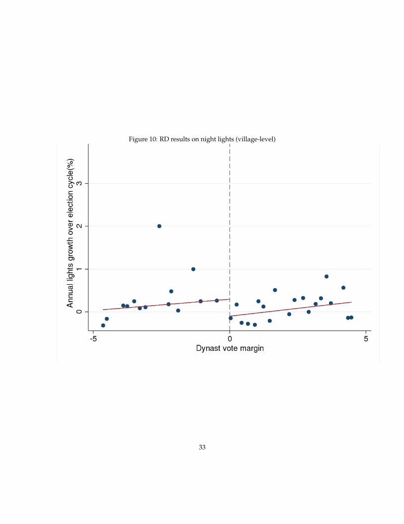
Figure 10: RD results on night lights (village-level)

33

Figure 11: RD result on night lights (village-level) w/different bandwidths

34

Figure 12: RD result on night lights (village-level) w/ FEs

35

Figure 13: Placebo RD – village level

36

Figure 14: Candidate balance – Education

37

Figure 15: Candidate balance – Education (different bandwidths)

38

Figure 16: Candidate balance – criminality

39

Figure 17: Candidate balance – criminality (different bandwidths)

40

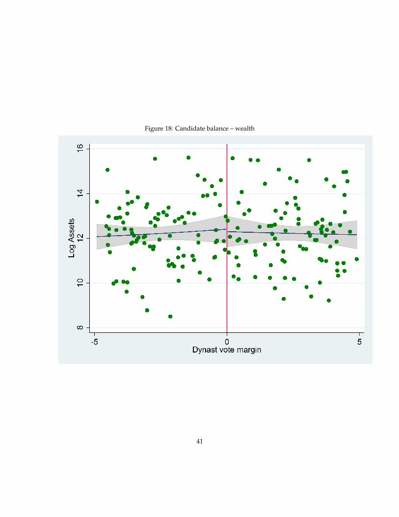
Figure 18: Candidate balance – wealth

41

Figure 19: Candidate balance – wealth (different bandwidths)

42

Figure 20: Mechanism – political competition (# of candidates in next election)

43

Figure 21: Mechanism – political competition (vote margin in next election)

44

Figure 22: Mechanism – rent seeking (asset gain between election cycles)

45

Figure 23: Mechanisms – politician effort (attendance in Parliament)

46

Figure 24: Mechanisms – politician effort (questions asked in Parliament)

47

Figure 25: Mechanisms – politician effort (participation in parliamentary debates)

48

Figure 26: Mechanisms – politician effort (introduced private member bill)

49

Figure 27: Parliamentary effort index

50

Figure 28: Do non-marginal dynasts perform well?

51

Figure 29: Do non-marginal dynasts perform well?

52

Figure 30: Dynastic performance across the distribution

53

Figure 31: Dynastic performance across the distribution

54

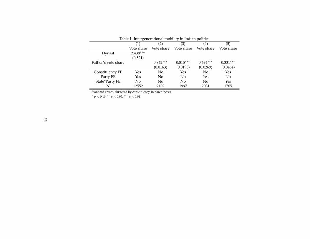
Table 1: Intergenerational mobility in Indian politics(1) (2) (3) (4) (5)

Vote share Vote share Vote share Vote share Vote shareDynast 2.438∗∗∗

(0.521)Father’s vote share 0.842∗∗∗ 0.815∗∗∗ 0.694∗∗∗ 0.331∗∗∗

(0.0163) (0.0195) (0.0269) (0.0464)Constituency FE Yes No Yes No Yes

Party FE Yes No No Yes NoState*Party FE No No No No Yes

N 12552 2102 1997 2031 1765Standard errors, clustered by constituency, in parentheses∗ p < 0.10, ∗∗ p < 0.05, ∗∗∗ p < 0.01

55

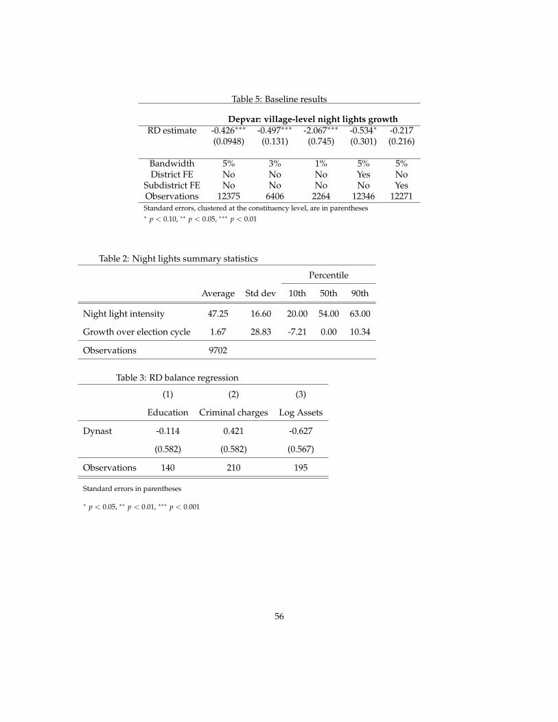
Table 5: Baseline results

Depvar: village-level night lights growthRD estimate -0.426∗∗∗ -0.497∗∗∗ -2.067∗∗∗ -0.534∗ -0.217

(0.0948) (0.131) (0.745) (0.301) (0.216)

Bandwidth 5% 3% 1% 5% 5%District FE No No No Yes No

Subdistrict FE No No No No YesObservations 12375 6406 2264 12346 12271Standard errors, clustered at the constituency level, are in parentheses∗ p < 0.10, ∗∗ p < 0.05, ∗∗∗ p < 0.01

Table 2: Night lights summary statistics

Percentile

Average Std dev 10th 50th 90th

Night light intensity 47.25 16.60 20.00 54.00 63.00

Growth over election cycle 1.67 28.83 -7.21 0.00 10.34

Observations 9702

Table 3: RD balance regression

(1) (2) (3)

Education Criminal charges Log Assets

Dynast -0.114 0.421 -0.627

(0.582) (0.582) (0.567)

Observations 140 210 195

Standard errors in parentheses

∗ p < 0.05, ∗∗ p < 0.01, ∗∗∗ p < 0.001

56

Table 4: Baseline results – night time lights growth

Night time lights growth

IK bandwidth (4.14) 50% IK 200% IK

Dynast -6.649∗ -6.572 -5.811∗

(3.464) (4.701) (3.025)

Observations 134

Standard errors, clustered at the constituency level, are in parentheses

∗ p < 0.10, ∗∗ p < 0.05, ∗∗∗ p < 0.01

57

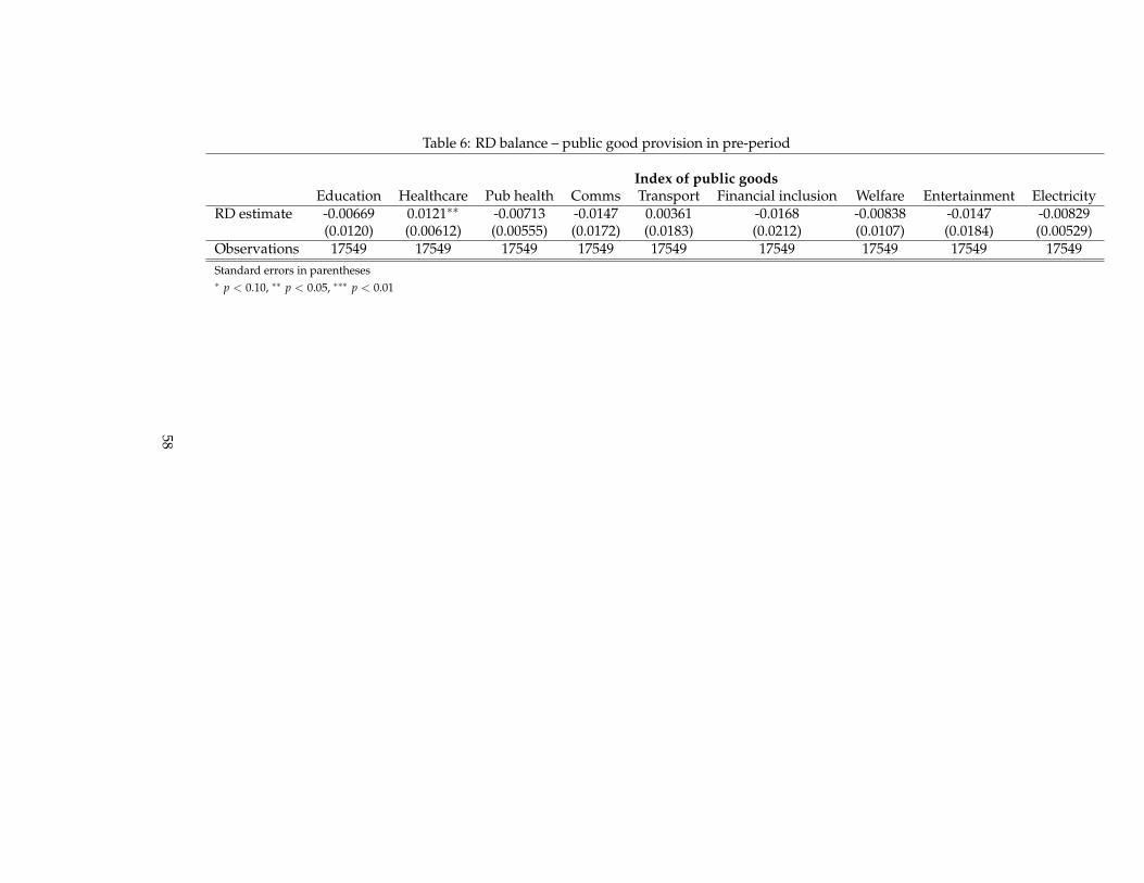
Table 6: RD balance – public good provision in pre-period

Index of public goodsEducation Healthcare Pub health Comms Transport Financial inclusion Welfare Entertainment Electricity

RD estimate -0.00669 0.0121∗∗ -0.00713 -0.0147 0.00361 -0.0168 -0.00838 -0.0147 -0.00829(0.0120) (0.00612) (0.00555) (0.0172) (0.0183) (0.0212) (0.0107) (0.0184) (0.00529)

Observations 17549 17549 17549 17549 17549 17549 17549 17549 17549Standard errors in parentheses∗ p < 0.10, ∗∗ p < 0.05, ∗∗∗ p < 0.01

58

Table 7: Impact of dynastic victory on public good provision

Index of public goods(1) (2) (3) (4) (5) (6) (7) (8) (9)

Education Healthcare Pub health Comms Transport Financial inclusion Welfare Entertainment ElectricityRD estimate -0.00414 -0.0784∗∗∗ -0.0283∗∗ 0.0173 -0.117∗∗∗ -0.107∗∗∗ -0.157∗ -0.108∗∗∗ -0.0465

(0.0330) (0.0184) (0.0138) (0.0180) (0.0398) (0.0231) (0.0952) (0.0351) (0.0307)

Eff. size in SD terms N/A 0.15 0.06 N/A 0.17 0.14 0.15 0.16 N/AObservations 3311 3311 3311 3311 3311 3311 3311 3311 3311Standard errors, clustered at constituency level, are in parentheses. All regressions include party and district fixed effects.∗ p < 0.10, ∗∗ p < 0.05, ∗∗∗ p < 0.01

59

Table 8: What issues do voters think are important? (Score 1-3)mean sd

1 Agricultural loan availability 0.98 1.112 Electricity for Agriculture 1.13 1.163 Better price-realization for farm products 1.20 1.284 Irrigation Programmes 1.09 1.205 Subsidy for seeds and fertilizers 1.08 1.226 Accessibility of MP 1.96 0.817 Anti-terrorism 2.07 0.718 Better employment opportunities 2.33 0.769 Better electric supply 2.20 0.7410 Better hospitals / Primary Healthcare Centres 2.15 0.8011 Better Law and Order / Policing 2.16 0.7812 Better public transport 2.26 0.7913 Better roads 2.22 0.7614 Better schools 2.16 0.8015 Drinking water 2.20 0.7716 Empowerment of Women 2.19 0.7817 Environmental issues 2.12 0.7818 Eradication of Corruption 2.09 0.8119 Reservation for jobs and education 2.12 0.7620 Security for women 2.17 0.7921 Strong Defence/Military 2.11 0.7822 Subsidized food distribution 2.15 0.8023 Training for jobs 2.14 0.7624 Trustworthiness of MP 2.09 0.8025 Other 1.10 1.1626 Better garbage clearance 0.57 0.9927 Encroachment of public land / lakes etc 0.57 0.9828 Facility for pedestrians and cyclists on roads 0.59 1.0229 Better food prices for Consumers 0.61 1.0530 Traffic congestion 0.59 1.03Average Importance of issue 2.19 0.40Observations 21531

60

Table 9: What issues do rural voters think are important? (Score 1-3)(1)

mean sd1 Agricultural loan availability 1.37 1.102 Electricity for Agriculture 1.52 1.113 Better price-realization for farm products 1.67 1.224 Irrigation Programmes 1.55 1.155 Subsidy for seeds and fertilizers 1.53 1.206 Accessibility of MP 2.00 0.797 Anti-terrorism 2.13 0.688 Better employment opportunities 2.42 0.689 Better electric supply 2.26 0.6810 Better hospitals / Primary Healthcare Centres 2.21 0.7711 Better Law and Order / Policing 2.21 0.7312 Better public transport 2.35 0.7213 Better roads 2.30 0.7014 Better schools 2.22 0.7615 Drinking water 2.28 0.7116 Empowerment of Women 2.25 0.7417 Environmental issues 2.18 0.7318 Eradication of Corruption 2.14 0.7819 Reservation for jobs and education 2.18 0.7120 Security for women 2.24 0.7321 Strong Defence/Military 2.19 0.7422 Subsidized food distribution 2.23 0.7523 Training for jobs 2.22 0.7124 Trustworthiness of MP 2.14 0.7625 Other 0.97 1.1726 Better garbage clearance 0.02 0.1927 Encroachment of public land / lakes etc 0.02 0.1928 Facility for pedestrians and cyclists on roads 0.02 0.2029 Better food prices for Consumers 0.02 0.2030 Traffic congestion 0.02 0.20Imp 2.23 0.38Observations 14539

61

Table 10: What issues do urban voters think are important? (Score 1-3)(1)

mean sd1 Agricultural loan availability 0.09 0.422 Electricity for Agriculture 0.20 0.633 Better price-realization for farm products 0.11 0.514 Irrigation Programmes 0.09 0.455 Subsidy for seeds and fertilizers 0.09 0.466 Accessibility of MP 1.93 0.787 Anti-terrorism 2.02 0.698 Better employment opportunities 2.23 0.799 Better electric supply 2.15 0.7610 Better hospitals / Primary Healthcare Centres 2.12 0.7911 Better Law and Order / Policing 2.14 0.7812 Better public transport 2.16 0.8113 Better roads 2.14 0.7614 Better schools 2.13 0.8115 Drinking water 2.13 0.7816 Empowerment of Women 2.14 0.7817 Environmental issues 2.06 0.8018 Eradication of Corruption 2.05 0.8119 Reservation for jobs and education 2.07 0.7620 Security for women 2.11 0.8021 Strong Defence/Military 2.02 0.7822 Subsidized food distribution 2.06 0.8023 Training for jobs 2.05 0.7624 Trustworthiness of MP 2.05 0.7825 Other 1.38 1.1026 Better garbage clearance 1.83 0.9327 Encroachment of public land / lakes etc 1.84 0.8628 Facility for pedestrians and cyclists on roads 1.91 0.9229 Better food prices for Consumers 1.98 0.9230 Traffic congestion 1.91 0.96Imp 2.14 0.38Observations 6390

62

Table 11: Voter assessment of politician performance (Score 1-3)mean sd

1 Agricultural loan availability 0.83 0.942 Electricity for Agriculture 0.94 1.013 Better price-realization for farm products 0.98 1.114 Irrigation Programmes 0.91 1.055 Subsidy for seeds and fertilizers 0.88 1.046 Accessibility of MP 1.52 0.707 Anti-terrorism 1.69 0.708 Better employment opportunities 1.72 0.819 Better electric supply 1.68 0.7310 Better hospitals / Primary Healthcare Centres 1.60 0.7511 Better Law and Order / Policing 1.66 0.7512 Better public transport 1.73 0.8013 Better roads 1.72 0.7514 Better schools 1.67 0.7715 Drinking water 1.70 0.7516 Empowerment of Women 1.71 0.7917 Environmental issues 1.65 0.7518 Eradication of Corruption 1.60 0.7619 Reservation for jobs and education 1.64 0.7420 Security for women 1.68 0.7921 Strong Defence/Military 1.66 0.7522 Subsidized food distribution 1.66 0.7823 Training for jobs 1.66 0.7624 Trustworthiness of MP 1.65 0.7725 Other 0.96 1.0526 Better garbage clearance 0.46 0.8227 Encroachment of public land / lakes etc 0.50 0.8728 Facility for pedestrians and cyclists on roads 0.50 0.8929 Better food prices for Consumers 0.49 0.8730 Traffic congestion 0.48 0.88Perf 1.72 0.47Observations 21531

63

Table 12: Voter assessment of politician performanceSample All voters Voter different caste to MP Voter same caste as MPDynast -0.280∗∗ -0.375∗∗∗ -0.149

(0.127) (0.137) (0.104)Observations 16731 9410 6167Standard errors, clustered at the constituency level, are in parentheses.All regressions include party and state FEs and controls for constituency and respondent characteristics.∗ p < 0.10, ∗∗ p < 0.05, ∗∗∗ p < 0.01

64

Table 13: Impact of dynastic victory on voter assessment of politician performanceDependent variable: voter assessment of MP performance

Sample Male Female Rural Urban Uneducated Educatedlwald -0.448 -0.360 -0.488 -0.249 -0.369 -0.217

(0.277) (0.311) (0.349) (0.233) (0.367) (0.343)Observations 14522 6753 14539 6390 8957 3008Standard errors in parentheses∗ p < 0.10, ∗∗ p < 0.05, ∗∗∗ p < 0.01

65

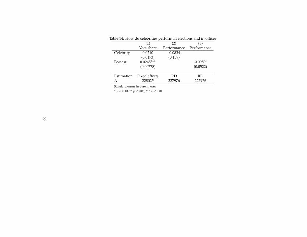
Table 14: How do celebrities perform in elections and in office?(1) (2) (3)

Vote share Performance PerformanceCelebrity 0.0210 -0.0834

(0.0173) (0.159)Dynast 0.0245∗∗∗ -0.0959∗

(0.00778) (0.0522)

Estimation Fixed effects RD RDN 228025 227976 227976Standard errors in parentheses∗ p < 0.10, ∗∗ p < 0.05, ∗∗∗ p < 0.01

66

Table 15: How do immediate family compare to other dynasts?(1) (2) (3)

All dynasts Son/Daughter/Wife Other dynastsWins close election -0.0959∗ -0.146∗∗ 0.00388

(0.0522) (0.0625) (0.0664)N 227976 140978 79453Standard errors in parentheses∗ p < 0.10, ∗∗ p < 0.05, ∗∗∗ p < 0.01

67

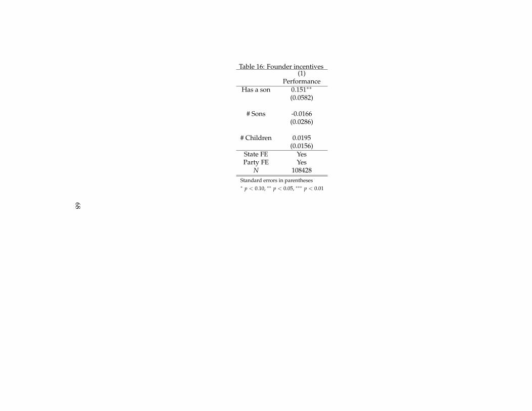
Table 16: Founder incentives(1)

PerformanceHas a son 0.151∗∗

(0.0582)

# Sons -0.0166(0.0286)

# Children 0.0195(0.0156)

State FE YesParty FE Yes

N 108428Standard errors in parentheses∗ p < 0.10, ∗∗ p < 0.05, ∗∗∗ p < 0.01

68