how do macroeconomic announcements impact the german …efujii/zhang.pdfhow do macroeconomic...
TRANSCRIPT

1
How do macroeconomic announcements impact the
German stock market?
Qunzi Zhang1
Abstract Based on a state-dependent FFF (Fourier Flexible Form) model, this paper investigates the scheduled
macroeconomic announcement effects on the five-minute return volatilities of three German stock indices: DAX, MDAX and SDAX, within a period from January 2007 until May 2008, which can be divided into two phases: a normal economic phase and the Subprime Crisis starting from July 2007. By using two kinds of comparative approaches, a cross-section analysis has been performed to investigate stock indices’ reactions to macroeconomic announcement surprises, which represent the news surprise sensitivity of each stock market segment. A finding shows that the DAX index has the strongest reaction to the news surprises. Additionally, this research work also investigates the high frequency volatility’s intraday properties, including intraday seasonality and long memory, which have important implications for the financial pricing of related instruments.
Field of Research: Financial Market, Financial Econometrics, Macroeconomic Announcement Effect
Keywords: Macroeconomic Announcements; High Frequency Data Analysis; Long Memory Modeling; Financial Stock Market
JEL Codes: G14, G15, G18
1 Introduction
Over the last two decades, many literatures have been focused on the realized volatility in the financial market, with a purpose of improving the development of the asset pricing process. Among these, French and Roll (1986) firstly state that the public information is one of the important candidates to price the volatility in US stock market. Afterwards, many research works have been focused on public information effects, i.e. macroeconomic announcement effects, in the financial market and revealed lots of meaningful results. Andersen and Bollerslev (1998), Anderson, Bollerslev, Diebold and Vega (2002), and among others, have revealed a significant news impact on the foreign exchange market;
1 Qunzi Zhang, School of Economics, Shandong University, Jinan Shandong, China, Email : [email protected]

2
there also exist a large number of papers focused on the bond markets, such as Fleming and Remolona (1997, 1999), Bollerslev, Cai and Song (2000), Balduzzi, Eltoon and Green (2001). For the stock market, as noted by Flannery and Protopapadakis (2002)1, “the hypothesis that the macroeconomic developments exert important effects on equity returns has strong intuitive appeal but little empirical support.” But they still stress “macro news, which can affect the overall business world reaction, must have the appealing power to explain the volatility in stock markets”. Chen, Roll, and Ross (1986) begin to support this hypothesis by testing the stock price’s response to expected or unexpected changes in the macroeconomic factors. Mitchell and Mulherin (1994) state that number of announcements released daily has significant relationship with aggregate measures of stock market activity including trading volume and market returns; Nikkinen and Sahlstroem (2004) find the effect of scheduled domestic and US macroeconomic announcement on German and Finnish equity markets, and their results show that the US macroeconomic announcement is even more important than the domestic announcement. However, “these studies above are relied on daily data” as noted by Harju and Hussain (2005), who build their work based on the high frequency data set and find the US macroeconomic news effects on the European stock markets (France, the UK, Switzerland, and Germany) are dominant and immediately. Therefore, as an extension of those scant but growing literatures, this present research tests US and Germany’s scheduled macroeconomic announcement effects on high frequency data in order to investigate the immediate response of the stock market. Since 1980s2, the increasingly existing high frequency data help the researchers to identify the intraday property of asset prices in a more refined way and many investigations are based on the empirical evidence of the intraday pattern of realized volatility in the financial markets. Jain and Joh (1988), Mclnish and Wood (1992), have found some intraday patterns, like U-shape intraday volatility. Then as noted by many researchers including Andersen and Bollerslev (1997), the intraday pattern should be eliminated from the time series in order to get the better estimation. Therefore, Andersen, Bollerslev, Diebold, Labys (2003) introduce a method to represent the intraday seasonality by a seasonal factor, which is used to get rid of the seasonal component in volatility. However, when the announcement effects are taken into account as mentioned above, a more refined approach to model the intraday seasonality is introduced by Anderson and Bollerslev (1998), i.e. Fourier Flexible Form (FFF).3 Following this method, this present work also models the five-minunte return volatility based on the FFF. In the modeling process, the Subprime Crisis starting from July 2007, which exists during the sample period here, should be taken into account. This ongoing worldwide economic problem has a large impact on the world financial markets. Among those, the most important and active stock market in Germany, Frankfurt Stock Exchange (FSE) has also been reeling under this special period. Based on this effective German stock market, a test for the scheduled macroeconomic announcement effects under Subprime Crisis will be quite appealing. Therefore, the state-depend dummy variables, which can represent the financial

3
situations in US and Germany, are included in a two-step FFF regression model. Additionally, as extension of the intraday property investigation, the long memory property4 will also be explored after filtering the intraday pattern and announcement effects away from the high frequency data. After conducting an estimation based on this state-dependent two-step FFF model, this present research aims to investigate the different stock indices’ reactions to the macroeconomic announcements, including DAX, MDAX and SDAX and answer the question “Which stock index is more sensitive to the news surprise?” For this purpose, two comparative methods are used to compare the stock indices’ news surprise sensitivities. This present work will contribute to the existing work in four ways: 1. Reveal the intraday properties in the volatility of three German stock indices, like intraday seasonality and long memory; 2. Analyze the US and Germany’s announcement effects based on high frequency data; 3. Concerning the large impact of Subprime Crisis, taking the economic state into account by introducing the state-dependent dummies is quite necessary and meaningful 4. To my own knowledge, there is no previous research into the cross-section study of the stock market’s reaction to announcement effects using these two comparative approaches. The organization of this present work is as follows. In section 2, the high frequency stock indices data and announcement data will be described. The intraday seasonality underlying the high frequency data will also be investigated. Section 3 summarizes the empirical results based on the state-dependent FFF regression model, and then the announcement effects and the long memory property will be addressed. Section 4 conducts the cross-section analysis based on the FFF model’s regression results, using two kinds of comparative methods. Section 5 concludes this work along with some ideas for future studies.
2 Data and Modeling 2.1 Stock indices data
The intraday high frequency data ticked by second are provided by the Deutsche Boerse AG5, covering three major stock indices DAX, MDAX and SDAX which represent different levels of capitalization in the German stock market6. The data sample is ranging from January 2nd, 2007 till May 30th, 2008, i.e. 357 trading days. The opening time in FSE is from 9:00 till 17:30, therefore, normally, there exist in total 102 five-minute intervals within each trading day, i.e. n=1,2,…N, where N=102. However, in some cases, the indices data existing start from 9:05 am, 9:10 am, 9:15 am, 9:20 am, or 9:25 am, and on 28th December 2007, for DAX, MDAX and SDAX, the market closes at 14:15, which make N equal to different values7. Therefore, in the end, there are in total 36314, 36339 and 36327 high frequency five-minute return observations for DAX, MDAX and SDAX indices.
4
2.11 Data Transformation The high frequency five-minute return and volatility can be calculated by taking the
interpolated logarithmic average of the two closest price happened around the five-minute point, as Mueller et al. (1990) and Dacorogna et al. (1993) did. However, since the data here are accurate to the second level, I directly use the price on each five-minute point instead of the approximate value calculated as above. After drawing the five-minute price from the raw data, I constructed the five-minute return, rt,n, according to the method used by Andersen et al. (2003), which is shown in formula 1, where t=1, 2, …357 trading days; n notes the five-minute interval, n=1, 2,….N, where N varies among three indices on different trading days.
t,n t,n t,nr log( ) log( )= -price price 1( )
According to the proposition of Andersen et al. (2003), depicted in formula 2, when the frequency becomes extremely high, namely the frequency’s time length Δ close to zero, the volatility will almost converge to “quadratic variation “, i.e. the square of the high frequency return.
t,n t,n t,n1
- , - ,,... /
´V r r= =n t j n t jj h
R R
2( )
where the rt,n+Δ and Vt,n are the high frequency five-minute return and volatility on day t. For
example in this present work, for most trading days, there are 102 five-minute intervals for each day, i.e. n=1, 2, 3…102, and Δ=1/102 0.00980392, and T=Δ,2Δ,3Δ…..36314 (DAX)8. The construction of five-minute volatility is as follows:
t,n t,n t,n t,nV r r r 2´= = 3( )
2.12 Intraday Seasonality
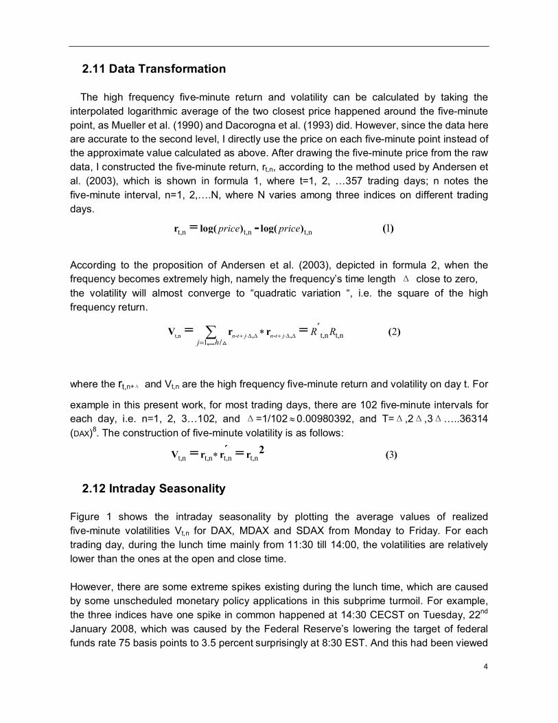
Figure 1 shows the intraday seasonality by plotting the average values of realized five-minute volatilities Vt,n for DAX, MDAX and SDAX from Monday to Friday. For each trading day, during the lunch time mainly from 11:30 till 14:00, the volatilities are relatively lower than the ones at the open and close time. However, there are some extreme spikes existing during the lunch time, which are caused by some unscheduled monetary policy applications in this subprime turmoil. For example, the three indices have one spike in common happened at 14:30 CECST on Tuesday, 22nd January 2008, which was caused by the Federal Reserve’s lowering the target of federal funds rate 75 basis points to 3.5 percent surprisingly at 8:30 EST. And this had been viewed

5
as a reaction to a new panic in the already sensitive market in Subprime Crisis, which is the French Bank Société Générale’s $7.2 billion loss, the biggest ever due to a rogue trader. Also another common spike happened around 14:30 CET in DAX, MDAX and SDAX, on Friday 17th August 2008, which was caused by a sudden cut of the primary credit discount window facility by the Federal Reserve at 8:30 EDT9. These two special days can be seen in graphs of Tuesday and Friday in Figure 1a, 1b and 1c. Additionally, according to Chang et al. (1999)10 and Pericli et al. (1997)11, trading of indices’ futures and options can increase the volatility of the stock market, here in this present work, some largest volatility can be explained by this reason. For example in Figure 1a, around 12:55 and 13:00, on Thursday, 20th March 2008, it is the close time for the last trading day of DAX@Futures, DAX@Options which is just correspondent to the largest five-minute volatility of DAX index. And this can also explain DAX index’s large fluctuation during the 48th five-minute interval (from 12:55 till 13:00) in Fridays corresponding to 21st December 2007 and 16th May 2008, which are shown by Graph of Friday in Figure 1a.
DAX intraday pattern from Monday to Friday (Figure 1a)
MDAX intraday pattern from Monday to Friday (Figure 1b)
6
SDAX intraday pattern from Monday to Friday (Figure 1c)
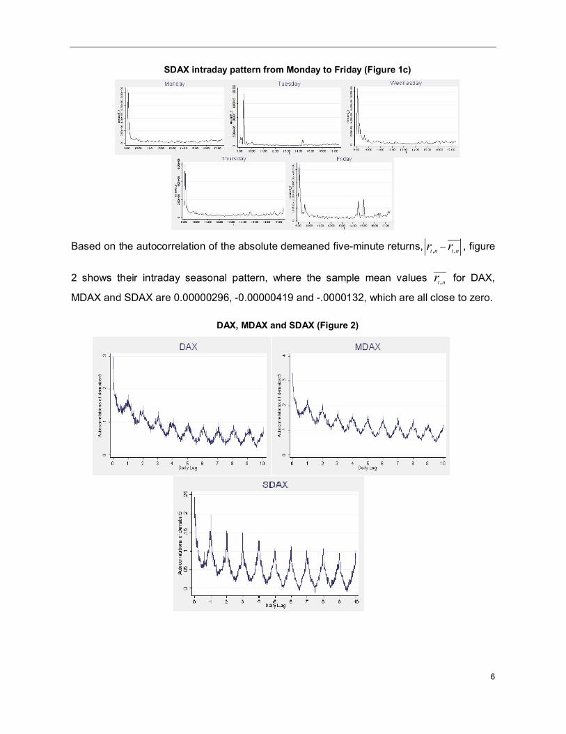
Based on the autocorrelation of the absolute demeaned five-minute returns, , ,t n t nr r , figure
2 shows their intraday seasonal pattern, where the sample mean values ____
,t nr for DAX,
MDAX and SDAX are 0.00000296, -0.00000419 and -.0000132, which are all close to zero.
DAX, MDAX and SDAX (Figure 2)

7
2.2 Announcement Data In order to investigate the immediate impact of the scheduled announcements, the exact release dates and times are needed. Here, the information about the announcement value and release schedule, is provided by nine economic institutions, including Bureau of Labor Statistics (BLS), Bureau of the Census (BC), Bureau of Economic Analysis (BEA), Federal Reserve Board (FRB) and Conference Board (CB), which are from US; the German institutions are the German Federal Statistical Office (GFSO, Statistisches Bundesamt Deutschland), Federal Labor Office (FLO, Bundesanstalt fuer Arbeit), and German Federal Bank (Deutsche Bundesbank). The information of M1, M3, i.e. Germany’s contribution in Eurozone money supply is provided by European Central Bank (ECB). Table 1 below summarizes the 32 kinds of scheduled macroeconomic announcements.
US and German Announcements from Jan 2007 till May 2008 (Table 1)
US Macroeconomic Announcements(Part A)
Announcement Obs.
Source Release Dates ReleaseTime(CET)
Quarterly Announcements 1.GDP Advance 6 BEA 31Jan07-30Apr0
8 14:30
2.GDP Preliminary 6 BEA 28Feb07-29May08
14:30
3.GDP Final 5 BEA 29Mar07-27Mar08
14:30/13:3012
Monthly Announcements 4.Industrial Production 1
7 FRB 17Jan07-15May0
8 15:15/14:1513
5.Capacity Utilization 17
FRB 17Jan07-15May08
15:15/14:1514
6.Consumer Credit 17
FRB 09Jan07-08May08
9:00
7. PPI 17
BLS 17Jan07-20May08
14:30/13:3015
8.CPI 17
BLS 18Jan07-14May08
14:30/13:3016
9.Import Price Index 17
BLS 12Jan07-13May08
14:30/13:3017
10.Unemployment Rate 17
BLS 05Jan07-02May08
14:30

8
11.Employment Cost Index 6 BLS 31Jan07-30Apr08
14:30/13:3018
12.Personal Income 17
BEA 01Feb07-30May08
14:30/13:3019
13.Personal Consumption and Expenditure
17
BEA 01Feb07-30May08
14:30/13:3020
14.Retail Sales 17
BC 14Jan07-12May08
14:30/13:3021
15.New Home Sales 17
BC 26Jan07-27May08
16:00/15:0022
16.Durable Goods Orders 17
BC 26Jan07-28Mayy08
14:30/13:3023
17.Construction Spending 17
BC 03Jan07-01May08
16:00/15:0024
18.Hausing Starts 17
BC 18Jan07-16May08
14:30/13:3025
19.ConsumerConfidenceIndex
17
CB 30Jan07-27May08
16:00/15:0026
20.Whole Sales 17
BC 10Jan07-8May08 16:00/15:0027
Weekly Announcements 21.Money Supply M1 7
4 FRB 05Jan07-29May0
8 9:00
German Macroeconomic Announcements(Part B)
Quarterly Announcements 22.Real GDP 6 GFSO 13Feb07-15May
08 8:00
Monthly Announcements 23.Employment 1
7 FLO 31Jan07-29May0
8 10:00
24.Current Account 17
DB 10Jan07-9May08 11:00
25.Producer Price 17
GFSO 22Jan07-20May08
8:00
26.Production Index 17
GFSO 09Jan07-08May08
12:00
27.Consumer Price 17
GFSO 17Jan07-15May08
8:00
28.Whole Sales Price Index 17
GFSO 10Jan07-09May08
8:00

9
29.Whole Sale Trade 17
GFSO 30Jan07-29May08
8:00
30.New Order Index 17
GFSO 08Jan07-07May08
12:00
31.Money Supply M1 17
ECB 26Jan07-29May08
10:00
32.Money Supply M3 17
ECB 26Jan07-29May08
10:00
2.21 Standardized Announcement Data
In order to analyze the announcement effects, here I use the surprise part of the scheduled announcements, i.e. the difference between the realized announcement value and expected announcement value, defined by Balduzzi et al. (2001). Because units of measurements of these surprise parts varies among different macroeconomic announcement values, the surprise part of the announcement needs to be standardized first before introduced into the estimation equation. According to the method of Balduzzi (2001), the standardized surprise is constructed as following:
k , t k , tk , t
k
A ES
4( )
Where Akt is the announced value of indicator k, Ekt is the market expected value of indicator
k and constant k
is the sample standard deviation of Akt-Ekt.
In this present work, the US announcement surprise data are from Thomson Financial IFR economist survey of Wall Street economists, which has been conducted every week since 1992. The purpose of this survey is to calculate the median forecast value (Ekt) of the economists’ expectations about the upcoming macroeconomic announcements and to get the announcement surprise (Akt-Ekt), which is the difference between the announcement value and the median forecast value; For the German announcements, however, because of the lack of survey data, I establish 11 econometric models separately for each German announcement time series and make one-step-ahead forecast in order to get the expectation value (Ekt), which can be used to calculate the German announcement surprise (Akt-Ekt)28. According to Bollerslev (2000) the standardized announcement surprise is zero when there is no announcement released. Here table 2 summarizes the statistical description about the standardized announcement surprises for US and Germany. The mean values for the standardized surprises are almost equal to zero for all the cases, supporting that the IFR survey data of the upcoming announcements and the forecasting value based on econometrics technique are pretty close to the true announcement value.

10
Standardized Announcement Surprise (US and Germany) (Table 2)
US announcement surprise Mean Std.Dev. Min Max 1.GDP Advance .0000583 .010705 -.9768
487 1.139657
2.GDP Preliminary .0000291 .0117662 -1.056971
1.585456
3.GDP Final .0001629 .0158067 0 1.971998
4.Industrial Production .0000288 .0281793 -2.092853
2.441662
5.Capacity Utilization -.0000361 .0211916 -1.637733
2.292827
6.Consumer Credit .0000751 .0183983 -1.336256
1.763116
7. PPI -.000131 .0341757 -6.242383
.891769
8.CPI -.0000561 .016897 -2.036453
1.018226
9.Import Price Index .0002034 .0198649 -.9632829
1.926566
10.Unemployment Rate -.0000191 .0150183 -1.388214
1.388214
11.Employment Cost Index -.0000615 .0062046 -.8938148
0
12.Personal Income .0000177 .0163559 -1.285884
2.250297
13.PersonalConsumption&Expenditure .0001144 .0203839 -1.038152
2.59538
14.Retail Sales -.0001097 .0158911 -1.742464
1.244617
15.New Home Sales -.0001149 .02013 -2.059089
1.694896
16.Durable Goods Orders -.0000607 .0202767 -1.861337
1.654522
17.Construction Spending .0000258 .0124518 -1.041547
.8332379
18.Hausing Starts -.0000103 .0197612 -2.241427
1.074017

11
2.3 State-dependent Modeling
Following the method used by Andersen et al. (1998) with a small amendment in the state-dependent part, the establishment of the estimation equation is as follows: Firstly, according to Andersen et al. (1998), the five-minute return can be decomposing as following:
t,n t,n t,n t,n t,n( )r E r s Z 5( )
19.ConsumerConfidenceIndex -.0000151 .0186947 -1.79205
1.602304
20.Whole Sales .0002055 .0257212 -1.447823
2.561532
21.Money Supply M1 .000529 .0592903 -1.331565
8.35
German Announcement Surprise
22.Real GDP .0000352 .0060312 -.3204286
1.033107
23.Employment .0002111 .0231443 -1.153515
2.073649
24.Current Account .0000247 .0215099 -1.232875
2.525534
25.Producer Price -6.91e-07 .0111924 -1.017879
1.249005
26.Production Index .0001592 .0168087 -.8933823
1.76723
27.Consumer Price 0.0052420 0.183734 -1.754104
2.759496
28.Whole Sales Price Index .0000968 .0157414 -.9957048
2.045224
29.Whole Sale Trade .0010046 .0605784 0 8.7
30.New Order Index .000063 .0180213 -1.426224
2.68849
31.Money Supply M1 .0000236 .022692 -2.449339
1.803644
32.Money Supply M3 .0000548 .022407 -2.095179
1.834805

12
Where t,n( )E r represent the expected value of five-minute return sample, which can be seen
equal to the sample mean value; ,t ns notes the standardized announcement
surprise; ,t n denotes the underlying daily volatility which can be estimated from conditional
volatility models or directly calculated from the unconditional realized volatility models. ,t nZ ,
is the white noise as assumed. And then, formula 6 shows the relationship between the absolute demeaned five-minute return and the realized volatility, and eliminates the underlying persistent daily volatility according to Andersen et al. (1998). And then the dependent variable lnvv5 is constructed and can be estimated based on formula 7:
t ,n t,nt ,n t,n t,n
t t t
2
2 52 21 2
r rr r Vln ln ln ln v v
N N N
6( )
32
11
2 25 cos sin( , )
P
pkp p
p plnvv c I t n vcos n vsin nk k
N N
t,n( )
oD m 7( )
The indicator variable ( , )k
t nI represents the standardized announcement surprise during
five-minute interval n on day t. The cos-and-sin part is the so called FFF (Fourier Flexible Form) introduced by Gallant (1981), which can be used to model the intraday pattern of the absolute demeaned five-minute return. And here the vcosp and vsinp are the coefficients for the FFF. ( )D m is the state-dependent dummy variable, which represents the financial situation of US and Germany for each month, m, during the sample period. The state-dependent dummy variable is defined based on the US leading Index provided by Conference Board and the current survey of the Germany Service Business Tendency conducted by OECD. When the financial situation is better compared with the same period in the previous year, the dummy is set equal to zero. The two-step estimation method is conducted based on formula 8 at first. For day t, the
estimated value t
for the persistent underlying daily volatility ,t n is directly calculated
based on the realized five-minute volatility, as formula 8 shows:
13
t,n t,n t,n1 2 1 2
1 1( )
N N
n nN V N
8( )
In the second step, after eliminating the daily volatility from the absolute demeaned
five-minute return, , ,t n t nr r , the ordinary least squares (OLS) regression is run based on
formula 7, which can be called the FFF regression according to Andersen et al. (1998). 3 Empirical Results and Discussion 3.1 Announcement Effects
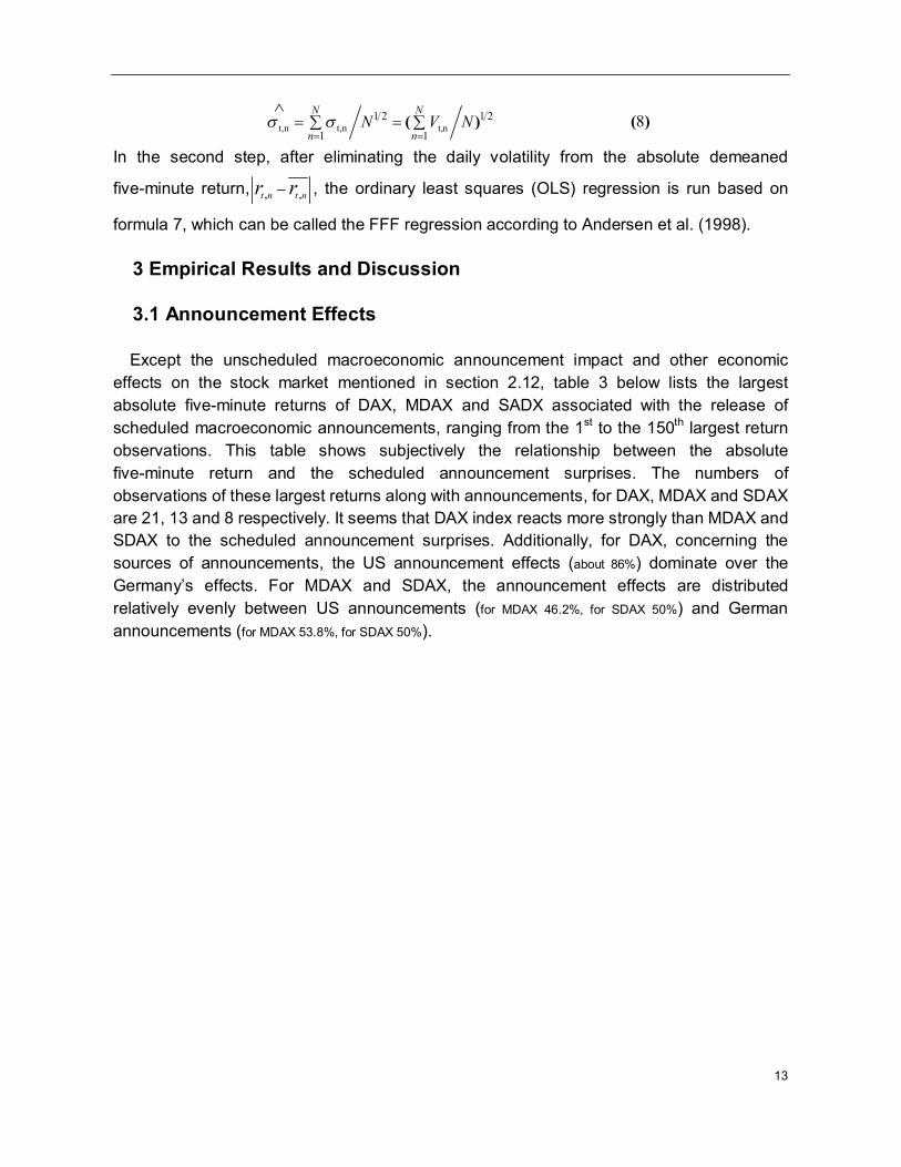
Except the unscheduled macroeconomic announcement impact and other economic
effects on the stock market mentioned in section 2.12, table 3 below lists the largest absolute five-minute returns of DAX, MDAX and SADX associated with the release of scheduled macroeconomic announcements, ranging from the 1st to the 150th largest return observations. This table shows subjectively the relationship between the absolute five-minute return and the scheduled announcement surprises. The numbers of observations of these largest returns along with announcements, for DAX, MDAX and SDAX are 21, 13 and 8 respectively. It seems that DAX index reacts more strongly than MDAX and SDAX to the scheduled announcement surprises. Additionally, for DAX, concerning the sources of announcements, the US announcement effects (about 86%) dominate over the Germany’s effects. For MDAX and SDAX, the announcement effects are distributed relatively evenly between US announcements (for MDAX 46.2%, for SDAX 50%) and German announcements (for MDAX 53.8%, for SDAX 50%).

14
Largest Absolute Five-minute return and Announcements (Table 3)
Absolute Return
Date Time
Announcement (US: U Germany: G)
DAX INDEX [Obs.: 21 (G:3 U:18)] .00945 31Jan08 14:30 Personal Income & personal consumption (U) .0081959 02May08 14:30 Unemployment (U) .0081463 09Mar07 14:30 Unemployment (U) .0078297 01Feb08 9:00 Money Supply M1 (U) .0076427 31Jan08 10:00 Employment & Whole Sale Price Index (G) .0071878 09Nov07 9:00 Money Supply M1 (U) .0071001 28Feb08 9:00 Consumer Credit & Money Supply M1(U) .006978 01Feb08 16:00 Construction Spending (U) .0069323 04Apr08 14:30 Unemployment (U) .006319 02May08 9:00 Money Supply M1 (U) .0062351 14Mar08 13:30 Retail Sales (U) .0060101 13Aug07 9:00 Whole Sale Price Index (G) .0058565 31Mar08 9:00 Whole Sales Trade (G) .0057764 14Mar08 14:45 Housing Starts (U) .0056982 27Apr07 14:30 GDP Advance (U) .0056725 04Jan08 14:30 Unemployment (U) .0054102 15Jun07 14:30 CPI (U) .0054054 24Apr07 16:00 Consumer Confidence Index (U) .0052032 24Apr08 14:30 Durable Goods Order (U) .0051279 08Nov07 9:00 Consumer Credit (U) .0050421 22Feb08 9:00 Money Supply M1 (U) MDAX INDEX [Obs.: 13(G:7 U:6)] .0096302 04Jan08 14:30 Unemployment (U)

15
Based on the FFF regression result, the announcement effects can be investigated in a more refined way. Here table 4 below summarizes the FFF regression result, of which the estimation is based on the robust standard errors in order to make sure that the estimation result will not be badly affected by outlying or aberrant observations in the data-set, especially during such a special Subprime Crisis period. The regression results show that for DAX, there are 11 announcement surprises effects are significant (most of them are significant at 5%
level). Compared to MDAX and SDAX, it seems that the DAX index are more sensitive to the announcement surprises, because the overall announcement effects on DAX index are more significant and it has the largest number of significant announcements. The state-dependent dummy variables have their interaction terms, however, only one of which is significant in the MDAX case. The intraday seasonality is exhibited by the FFF, including vsin and vcos parts. Here the lag value of vsin and vcos are decided according to the BIC and AIC information criteria, and the significant level of vsin’s or vcos’s coefficients. In order to conserve space, I only list in table 4 below the announcements of which the coefficients are significant.
.0086727 04Apr07 14:30 Unemployment (U)
.0081739 17Aug07 9:00 Producer Price (G)
.0081072 31Jan08 10:00 Employment (G)
.0072546 20May08 9:00 Producer Price (G)
.0072031 15Feb08 14:30 Import Price Index (U)
.0068111 08Jun07 9:00 Consumer Credit & Money Supply M1(U)
.0067511 31Jan08 14:30 Personal Income & personal consumption (U)
.0064716 20Nov08 9:00 Producer Price (G)
.0062637 14Feb08 9:00 GDP real (G)
.0061092 31Mar08 9:00 Whole Sales Trade (G) .005929 14Mar08 13:30 Retail Sales (U) .0058908 16Jan08 9:00 Consumer Price (G)
SDAX INDEX[Obs.: 8(G:4 U:4) .0067072 08Jun07 9:00 Consumer Credit & Money Supply M1(U) .0054922 28Feb07 10:00 Employment (G) .0042744 15Feb08 14:30 Import Price Index (U) .0037117 08Aug07 9:00 Consumer Credit (U) .0034904 07Mar07 9:00 New Order Index (G) .0034637 30Aug07 9:00 Whole Sales Trade (G) .0031643 01Feb08 9:00 Money Supply M1 (U) .0030909 31Jan08 10:00 Employment (G)

16
Regression Result for the Announcement Immediate Impact (Table 4) Here * for p<0.15, ** for p<0.1, and *** for p<0.05.
DAX_FFFreg. Lnvv5 b/t
Germany Announcement M3 -0.614*
(-1.58) GDPreal -5.884***
(-7.99) Whole.S.P 1.885***
(3.85) Wholesaletrade 0.609***
(3.96) US announcements
GDPa 3.183*** (7.16)
GDPf 1.751*** (3.31)
Industr.Util. 1.354*** (2.93)
Capacit.Util. -1.796*** (-2.22)
Employ cost -3.415*** (-3.98)
Wholesales 0.410*** (1.96)
M1 0.427*** (3.38)
usdum0g1b -0.063*** (-2.33)
gerdum0g1b 0.159*** (3.96)
vcos1 0.501*** (28.67)
vcos2 0.097*** (5.57)
vcos5 0.032** (1.85)
vcos6 0.129*** (7.36)
vcos9 0.032**
MDAX_FFFreg. Lnvv5 b/t
Germany Announcement Prod.P. 1.588**
(1.90) Consumerpr 0.770***
(2.29) Wholesaletrade 0.522*
(1.51) Neworderindex 0.614*
(1.52) US announcements
GDPa 2.379*** (2.56)
PPI -0.220** (-1.66)
Employcost -2.701*** (-2.37)
Wholesales 0.761** (1.96)
gerdum0g1b -0.152*** (-2.77)
interUS_Ger 0.201*** (2.63)
vcos1 0.672*** (38.09)
vcos2 0.100*** (5.68)
vcos3 0.055*** (3.16)
vcos4 -0.037*** (-2.12)
vcos6 0.126*** (7.12)
vcos13 -0.046*** (-2.63)
vcos16 -0.063*** (-3.59)
vcos18 0.036***
SDAX_FFFreg. Lnvv5 b/t Germany Announcement
M3 -0.591* (-1.58) GDPreal 0.497**
-1.74 Productindex -2.361*** (-2.68)
US announcements GDPa 2.523***
-3.58 Employ cost -3.161*** (-3.99) Personal Income 0.589**
-1.85 M1 -0.980*** (-2.83) usdum0g1b 0.085***
-3.17 gerdum0g1b -0.241*** (-6.36) vcos1 0.481***
-28.18 vcos2 0.139***
-8.19 vcos3 0.122***
-7.15 vcos4 0.075***
-4.41 vcos5 0.063***
-3.67 vcos6 0.100***
-5.86 vcos11 0.033**
-1.9 vcos19 -0.034*** (-1.99) vsin1 0.066***

17
(1.82) vcos13 -0.035***
(-2.02) vcos14 0.038***
(2.20) vcos16 -0.046***
(-2.64) vcos18 0.027*
(1.57) vsin1 -0.240***
(-13.82) vsin4 0.046***
(2.67) vsin5 0.135***
(7.80) vsin7 -0.036***
(-2.05) vsin9 0.065***
(3.72) vsin11 0.038***
(2.14) vsin12 0.039***
(2.21) vsin13 0.066***
(3.82) vsin14 0.047***
(2.69) vsin17 0.151***
(8.64) vsin18 0.049***
(2.81) _cons -1.771***
(-44.62)
(2.07) vsin1 -0.081***
(-4.64) vsin2 0.069***
(3.93) vsin3 0.042***
(2.38) vsin4 0.132***
(7.51) vsin5 0.162***
(9.22) vsin6 0.080***
(4.59) vsin8 0.039***
(2.26) vsin9 0.124***
(7.06) vsin10 0.048***
(2.75) vsin11 0.076***
(4.32) vsin12 0.048***
(2.74) vsin13 0.061***
(3.47) vsin14 0.068***
(3.85) vsin17 0.119***
(6.78) vsin18 0.039***
(2.20) vsin19 0.046***
(2.63) _cons -1.735***
(-35.67)
-3.9 vsin2 0.085***
-4.95 vsin3 0.105***
-6.16 vsin4 0.044***
-2.59 vsin5 0.131***
-7.72 vsin6 0.073***
-4.3 vsin7 0.033**
-1.92 vsin8 0.042***
-2.48 vsin9 0.076***
-4.46 vsin10 0.075***
-4.46 vsin11 0.028*
-1.64 vsin12 0.027*
-1.59 vsin13 0.045***
-2.62 vsin14 0.061***
-3.59 vsin15 0.039***
-2.28 vsin16 0.066***
-3.85 vsin17 0.088***
-5.13 vsin18 0.060***
-3.5 vsin19 0.066***
-3.89 vsin20 0.031**
-1.84 _cons -1.414*** (-37.93)

18
Descriptive Statistics DAX MDAX SDAX
Adj. R-Square _N BIC AIC
0.036 36314.000 165481.422 165013.924
0.052 36339
166284.819 165774.780
0.035 36327.000 163927.133 163391.613
After running the FFF regression based on formula 7, the estimated value Fitted_lnvv5 and the true value lnvv5 which is on the left hand side of formula, are plotted in figure 3. The results show that the estimation models have predicted the fluctuation in DAX, MDAX and SDAX quite well.
FFF regression results (Figure 3)
-3-2
-10
1
0 20 40 60 80 100t
lnvv5 Fitted_lnvv5
DAX_FFFregression
-3-2
-10
1
0 20 40 60 80 100t
lnvv5 Fitted_lnvv5
MDAX_FFFregression
-3-2
-10
1
0 20 40 60 80 100t
lnvv5 Fitted_lnvv5
SDAX_FFFregression
Note: the value plotted here are the average per second.

19
3.2 Long Memory Property In this section I investigate the long memory property existing in the filtered absolute demeaned five-minute returns and the underlying daily volatility which drives this long memory process. Following Bollerslev et al. (2000), the fractionally integrated order d is estimated and the results here also support their findings. In order to investigate the long memory property of the absolute demeaned five-minute return, the intraday seasonality, state-dependent dummy effects and announcement effects should be filtered away at first29, according to formula 9 (Andersen et al. 1998):
t ,n t ,n
tnf i l t e r e d _ d e m e a n a b s r 5
2( / )
r r
e x p x
9( )
Here, Xtn is the estimated value for the right hand side of formula 7, which represents the estimated value for intraday seasonality, announcement effects and state-dependent dummy effects on the right hand side of formula 7. Figure 4 below is plotting the autocorrelogram for the absolute demeaned five-minute returns before and after this filtering process.
Intraday Seasonality & Announcement Filtered (Figure 4)
0.1
.2.3
0 1 2 3 4 5 6 7 8 9 10Daily Lag
AC_filtered_demeanabsr5 AC_demeanabsr5
DAX_filter_demeanedabsr5
0.1
.2.3
.4
0 1 2 3 4 5 6 7 8 9 10Daily Lag
AC_filtered_demeanabsr5 AC_demeanabsr5
MDAX_filter_demeanedabsr5
0.05
.1.15
.2.25
0 1 2 3 4 5 6 7 8 9 10Daily Lag
AC_filtered_demeanabsr5 AC_demeanabsr5
SDAX_filter_demeanedabsr5
Ten-day Correlogram for raw and filtered , ,t n t nr r according to Bollerslev (2000) Figure 2a.

20
From figure 4, we can see that after filtering out the intraday seasonality, announcement and
state-dependent dummy effects in the demeaned returns, , ,t n t nr r , the autocorrelogram
exhibits a slowly decaying pattern, namely, “hyperbolic decaying pattern”, which implies that there exists long memory property30. Several methods are frequently used for testing the long memory property and estimating the fractionally integrated order d, such as GPH (Geweke and Porter-Hudak 1983), MODLPR (Phillips 1999)31 and ROBLPR32 (Baum 2000a), etc. According to Baum (2000 b)33, MODLPR (the Phillips modified GPH log periodogram regression estimator) performs well in testing the stock returns time series and can automatically remove the deterministic trend in the series. Therefore, the MODLPR is used to conduct the long memory test and estimation for the
filtered , ,t n t nr r . The long memory testing results are summarized in table 5, where the null
hypothesis d=1 is significantly rejected at zero percent level, implying that there exists long
memory property in the filtered , ,t n t nr r .
Long memory testing results from MODLPR (Table 5)
Furthermore, according to Bollerslev et al. (2000), the underlying daily volatility actually causes the existing long memory in the demeaned high frequency returns. And they introduced a “time-domain-based” estimate method to predict the fractionally integrated order d.

21
This method assumes that the autocorrelations, n , satisfy 2 1n
dcn , when the lags n is
large enough. And c denotes a proportional factor. Taking logarithm on this formula yields formula 10:
n 2 1lo g lo g c d lo g n 10( )
Therefore based on formula 10, an OLS regression can be applied to the autocorrelations of
all the filtered , ,t n t nr r and then estimate the coefficients, (2d-1); meanwhile, the estimator of
integrated order d, acd
, can be also calculated. Here, the lags n=1, 2…N (N equals to 36314, 36339
or 36327 for three indices: DAX, MDAX and SDAX). The coefficients of independent variable log(n) are
the estimated values for (2d-1), from which the three acd s
for the three indices can be
easily calculate _ac DAXd
=0.2821768, _ac MDAXd
=0.29995675 and _ac SDAXd
=0.244275.The
OLS regression results for (2d-1) of the three indices are as following:
Autocorrelation Regression Estimator for d (Table 6)
Following Bollerslev et al. (2000), in figure 5 I also plot the results about the estimated decay
patterns of the autocorrelations of the filtered , ,t n t nr r , where 2 1dn notes this estimated
pattern. We can see that the estimated pattern’s decaying speed is quiet similar with the one
of the autocorrelation’s hyperbolic decaying pattern of the filtered , ,t n t nr r .

22
Estimated Decay for AC of , ,t n t nr r (Figure 5) 0
.2.4
.6.8
1
0 1 2 3 4 5 6 7 8 9 10Daily Lag
Estimated_decay AC_filtered_demeanabsr5
DAX
0.2
.4.6
.81
0 1 2 3 4 5 6 7 8 9 10Daily Lag
Estimated_decay AC_filtered_demeanabsr5
MDAX
0.2
.4.6
.81
0 1 2 3 4 5 6 7 8 9 10Daily Lag
Estimated_decay AC_filtered_demeanabsr5
SDAX
Here, Estimated_decay= 2 1dn .

23
In order to verify Bollerslev et al.’s OLS regression method, I also apply the MODLPR test to
the daily volatility, vd , where2
tvd
( t
is from formula 8). Although the sample size for the daily volatility is not large enough, which is only 357 days34, the estimated d values for DAX, MDAX and SDAX indices: .2298488, 0.2702292 and 0.2318864 are still almost
consistent with the acd
above ( _ac DAXd
=0.2821768, _ac MDAXd
=0.29995675
and _ac SDAXd
=0.244275). This result supports that the “time-domain-based” estimation
method can perform well in predicting the long memory property underlying the high frequency German stock returns and verifies that the persistent daily volatility causes the long memory.
MODLPR Estimation for Daily Volatility vd (Table 7)
4 Cross-section analyses In order to answer the question “Which stock index is more sensitive to the news surprise?”, two kinds of comparative approaches are used to check the different scheduled announcement effects on the three indices, including the volatility-ratio method used by Lyon et al. (1997) and coefficient-ratio method.

24
4.1 Volatility-ratio method
In order to compare the stock indices’ reactions to the scheduled announcements, three volatility ratios are established as following:
1 ( ) / ( )VolRatio Var DAX Var MDAX
2 ( ) / ( )VolRatio Var DAX Var SDAX
3 ( ) / ( )VolRatio Var MDAX Var SDAX
The volatilities used here are from the subsamples of the five-minute realized volatility, for which the macroeconomic announcement is released during this interval. Table 8a and 8b describe the three ratios based on two different kinds of subsamples: one includes all the five-minute volatilities when there are announcements released, the other comprises volatilities of three indices, for which every two of them have common significant announcement effects (according to the FFF regression results summarized in table 4). Here result in table 8a shows that, overall, the DAX index is most strongly affected by the announcements release (VolRatio 1 and 2 are greater than 1). The announcements exert the smallest effect on SDAX comparing to the other two indices (VolRatio 2 and 3 are smaller than 1). Since the standard deviation is quiet large here, the median value for the three ratios can be a better criteria to compare the stock indices’ reactions to announcements.
Three volatility ratios for DAX, MDAX, and SDAX (Table 8a_subsample 1)
Ratios Obs. Median Mean Std. Dev.
Min Max
VolRatio1
367 1.114644
30337.17
576755.9
.0000139
1.10e+07
VolRatio2
367 5.478537
261.5784
1769.285
.0001676
28443.44
VolRatio3
367 4.641767
340.8346
2811.383
2.96e-06
49535.17
Table 8b below summarizes the common significant announcement effects for each pair of stock indices and implies the same results as table 8a does.

25
Three volatility ratios for DAX, MDAX, and SDAX (Table 8b_subsample 2)
VolRatio1(DAX_MDAX) VolRatio2(DAX_SDAX) VolRatio3(MDAX_SDAX) Common Announcements
Wholesale trade(G) GDP advance(U) Employment cost
index(U) Wholesales(U)
M3(G) GDP real(G)
GDP advance(U) Employment cost index(U)
M1(U)
GDP advance(U) Employment cost index(U)
Note: (G) and (U) denote the Germany and US announcements.
Ratios Obs. Median Mean Std. Dev. Min Max VolRatio1 35 1.552612 16.347 55.85751 .01349 275.6209 VolRatio2 85 5.241531 105.309 348.5884 .00016 2146.576 VolRatio3 6 10.5302 84.38209 189.3293 .10114 470.6623
4.2 Coefficient-ratio method
The second approach is to compare the announcement variables’ explanatory power by calculating the ratios of their coefficients (according to the FFF regression results summarized in table 4). The coefficient ratios are constructed as following:
1 .( _ ) / .( _ )CoeRatio Coe Ann DAX Coe Ann MDAX
2 .( _ ) / .( _ )CoeRatio Coe Ann DAX Coe Ann SDAX
3 .( _ ) / .( _ )CoeRatio Coe Ann MDAX Coe Ann SDAX
Based on table 9, the mean values for three CoeRatios are 1.05785, 3.13112 and 0.898701. Only the CoeRatio3 is contradicting to result of the VolRatio3. However, based on the general results obtained from this cross-section analysis, I would say that the DAX index is most sensitive to the announcement effects, and MDAX responds more strongly to announcement releases than SDAX does.

26
Coefficient-ratio and Common Announcements (Table 9)
5 Conclusions and Perspectives
This paper aims to investigate the macroeconomic announcement effects on German stock market and deepen the understanding of the announcement impact through a cross-section analysis on the three representative stock indices, DAX, MDAX and SDAX. Based on a state-dependent Fourier Flexible Form model, the high frequency five-minute return has been decomposed into five parts: daily volatility persistency (long memory property), the announcement effects, intraday seasonality, state-dependent dummy effects and the white noise part. The results suggest that compared to the other two indices, DAX index reacts more strongly to the announcement surprises, especially to the US news. Additionally, some important intraday properties, such as intraday seasonality and long memory underlying the high frequency data, have been studied. The intraday seasonality has been explained through the plotting of weekdays’ graphs and high frequency data’s correlogram. And the long memory investigation is conducted following Bollerslev et al. (2000). Meanwhile, the OLS estimation method for integration order d has also been verified by the results of German stock indices.
Coef.
Index
Wholesal
e Trade
GDP
advance
Employme
nt Cost
Wholesales
DAX 0.609 3.183 -3.415 0.410
MDAX 0.522 2.523 -2.701 0.761
CoeRatio
1
1.1667 1.2616 1.2643 0.5388
Coef.
Index GDP real M3 GDP
advance
Employme
nt Cost
M1
DAX -5.884 -0.614 3.183 -3.415 0.427 SDAX 0.497 -0.591 2.523 -3.161 -0.980
CoeRatio2
11.839 1.0389 1.2616 1.0804 0.4357
Coef.
Index
GDP
advance
Employme
nt
cost
MDAX 2.379 -2.701 SDAX 2.523 -3.161
CoeRatio3
0.942925
0.854476

27
Although this present work has extended the growing literature of the scheduled macroeconomic announcement effects on stock market by using high frequency data of three German stock indices and conducting a cross-section analysis among three indices reactions to news surprises, there are still many interesting research directions for the future study. Firstly, as Bollerslev et al. (2000) study the bond market and Andersen et al. (2002) study the foreign exchange market, a dynamic announcement responds pattern can be applied into the study of the German stock market, in order to show the dynamic announcement effects during several five-minute intervals. Secondly, it will be of interest to conduct a comparison study on the announcement effects between the data samples from the good time and the bad time (Subprime Crisis) by extending the time period starting from 2005 or even earlier. Then the robustness of the model established in this work can be tested. Finally, the asymmetric announcement effects are also of interested to explore, since news effects usually varies with their signs, as Andersen et al. (2002) said “negative surprises often have greater impact than positive surprises.” References
Andersen, TG and Bollerslev, T 1997, Intraday periodicity and volatility persistence in financial markets, Journal of Empirical Finance, Elsevier, vol. 4(2-3), pages 115-158.
Andersen, TG and Bollerslev, T 1998, Answering the Skeptics: Yes, Standard Volatility
Models Do Provide Accurate Forecasts, International Economic Review, vol. 39(4), pages 885-905.
Andersen, TG, Bollerslev, T, Diebold, FX and Labys, P 2003, Modeling and forecasting realized
volatility, Econometrica, Volume 71 Issue 2, Pages 579 – 625. Andersen, TG, Vega, C, Bollerslev, T and Diebold, FX 2002, Microeffects of macro
announcements: real-time price discovery in foreign exchange, NBER Working Paper No. W8959.
Baillie, RT 1996, Long memory processes and fractional integration in econometrics,
Journal of Econometrics, 73 (1), pp. 5-59.

28
Balduzzi, P, Elton, JE and Green, TC 2001, Economic news and bond prices: evidence from the U.S. Treasury Market, The Journal of Financial and Quantitative Analysis, Vol. 36, No. 4, pp. 523-543.
Baum, CF and Wiggins, V 2000, ROBLPR: Stata module to estimate long memory in a set of timeseries, Statistical Software Components S411001.
Bhardwaj G, and Swanson NR 2006, An empirical investigation of the usefulness of ARFIMA models for predicting macroeconomics and financial time series, Journal of Econometrics, 131 (1-2), pp. 539-578.
Bollerslev T, Cai J, Song FM 2000, Intraday periodicity, long memory volatility, and macroeconomic announcement effects in the US Treasury bond market, Journal of Empirical Finance, 7 (1), pp. 37-55.
Chang E, Cheng J, Pinegar J 1999, Does futures trading increase stock market volatility?
The case of the Nikkei stock index futures markets, Journal of Banking and Finance 23(5):727-753.
Chen, NF, Roll, R and Ross, SA 1986, Economic Forces and the Stock Market, The
Journal of Business, Vol. 59, No. 3, pp. 383-403.
Dacorogna, MM, Muller, UA, Nagler, RJ, Olsen, RB and Pictet, OV 1993, A geographical model for the daily and weekly seasonal volatility in the foreign exchange market, Journal of International Money and Finance, Elsevier, vol. 12(4), pages 413-438.
Fleming, MJ and Remolona, EM 1997, What moves the bond market?, Economic Policy
Review, Vol. 3, No. 4.
Fleming, MJ and Remolona, EM 1999, Price formation and liquidity in the U.S. treasury market: the response to public information, Journal of Finance, American Finance Association, vol. 54(5), pages 1901-1915.
Flannery, MJ and Protopapadakis, AA 2002, Macroeconomic Factors Do Influence
Aggregate Stock Returns, Review of Financial Studies, vol. 15(3), pages 751-782. French, KR and Roll, R 1986, Stock return variances: The arrival of information and the
reaction of traders, Journal of Financial Economics, vol. 17(1), pages 5-26. Gallant, AR 1981, On the bias in flexible functional forms and an essentially unbiased
form: The fourier flexible form, Journal of Econometrics, vol. 15(2), pages 211-245.

29
Giot, P 1999, Time transformations, Intra-day data and volatility models, Journal of Computational Finance, 31--62
Harju, K und Hussain, SM 2005, Intraday Seasonalities and Macroeconomic News Announcements, WP, HANKEN-Swedish School of Economics and Business Administration, Vasa, Finland.
Ito, T, Lyons, RK and Melvin, MT 1998, Is There Private Information in the FX Market?
The Tokyo Experiment, The Journal of Finance, Vol. 53, No. 3, pp. 1111-1130. Jain, PC and Joh, GH 1988, The dependence between hourly prices and trading volume,
Journal of Financial and Quantitative Analysis, 23(3):269-283. Muller, UA, Dacorogna, MM,Olsen, RB, Pictet, OV, Schwarz, M and Morgenegg, C 1990,
Statistical study of foreign exchange rates, empirical evidence of a price change scaling law, and intraday analysis, Journal of Banking & Finance, vol. 14(6), pages 1189-1208.
Mitchell, ML and Mulherin, JH 1994, The Impact of Public Information on the Stock
Market, Journal of Finance, American Finance Association, vol. 49(3), pages 923-50. McInish, TH and Wood, RA 1992, An Analysis of Intraday Patterns in Bid/Ask Spreads for
NYSE Stocks, Journal of Finance, vol. 47(2), pages 753-64. Nikkinen, J and Sahlstrom, P 2004, Scheduled domestic and US macroeconomic news
and stock valuation in Europe, Journal of Multinational Financial Management, vol. 14(3), pages 201-215.
Pericli, A and Koutmos, G 1997, Index Futures and Options and Stock Market Volatility, Journal of Futures Markets 17(8):957-974.
Phillips, Peter CB 1999a, Discrete Fourier Transforms of Fractional Processes,
Unpublished working paper No. 1243, Cowles Foundation for Research in Economics, Yale University.
Phillips, Peter CB 1999b, Unit Root Log Periodogram Regression, Unpublished working paper No. 1244, Cowles Foundation for Research in Economics, Yale University.
1 According to Harju, K. und S.M. Hussain(2005) 2 According to “Market microstructure: A survey” by Ananth Madhavan. 3 The FFF is introduced by Gallant (1998).

30
4 The long persistence of the return volatility, called long memory property, is also a momentum for the high
frequency volatility and will be shown obviously after the intraday seasonality and the announcement effect are eliminated, reported by Bollerslev, Can, and Song (2000).
5 Deutsche Boerse AG operates the Frankfurt Stock Exchange, the largest of seven stock exchanges in Germany.
6 “The DAX reflects the segment of blue chips admitted to the Prime Standard Segment and comprises the 30 largest and most actively traded companies that are listed at the Frankfurt Stock Exchange; MDAX comprises 50 mid-cap issues from traditional sectors (“Classic”) which, in terms of size and turnover, rank below the DAX; The SDAX comprises the next 50 issues from the traditional (“Classic”) sectors within the Prime Standard Segment that are ranked below the MDAX.”—“Guide to the Equity Indices of Deutsche Boerse (2008)”
7 For DAX, there are 62 trading days starting after 9:05, where N=101; for MDAX, 24 days start after 9:05, i.e. N=101. 60 days begin after 9:10, where N=100. For SDAX, except 334 days which have 102 five-minute intervals, there are 15 days starting after 9:05, 6 days after 9:15, 1day after 9:20, 1day after 9:25 and 1 day ends at 14:15 on the same day as DAX and MDAX. For all these cases of SDAX, N=102, 101, 100, 99, 98, 63. For three indices, on 28th December 2007, there are only 63 five-minute returns exist, since the trading day ends at 14:15, where N=63.
8 There are 36339 observations for MDAX and 36327 for SDAX. 9 In order to improve the market liquidity during Subprime Crisis, the Federal Reserve reduced 50 basis
points in the primary credit rate to 3.75 percent and announced a change “to the Reserve Banks' usual practices to allow the provision of term financing for as long as 30 days, renewable by the borrower.”-Press release paper from Federal Reserve on 17th Aug 2008.
10 Chang E, Cheng J, Pinegar J. Does Futures Trading Increase Stock Market Volatility? The Case of the Nikkei Stock Index Futures Markets. Journal of Banking and Finance May 1999;23(5):727-753.
11 Pericli A, Koutmos G. Index Futures and Options and Stock Market Volatility. Journal of Futures Markets December 1997;17(8):957-974.
12 Because the different starting and ending time for the daylight saving time in Germany and US, the release time for the US announcements varies due to this difference between three periods: 11th March 2007 -25th March 2007, 28th October 2007-4th November 2007, 9th March 2008 30th March 2008.
13 On 16th March 2007, 17th March 2008, the time difference between US and Germany is 5 hours. 14 On 16th March 2007, 17th March 2008, the time difference between US and Germany is 5 hours. 15 On 18th March 2008, the time difference between US and Germany is 5 hours. 16 On 14th March 2008, the time difference between US and Germany is 5 hours. 17 On 13th March 2008, the time difference between US and Germany is 5 hours. 18 On 31st Oct. 2008, the time difference between US and Germany is 5 hours. 19 On 11th Nov. 2007, 28th March 2008, the time difference between US and Germany is 5 hours. 20 On 11th Nov. 2007, the time difference between US and Germany is 5 hours. 21 On 16th March 2007, 14th March 2008, the time difference between US and Germany is 5 hours. 22 On 26th March 2008, the time difference between US and Germany is 5 hours. 23 On 26th March 2008, the time difference between US and Germany is 5 hours. 24 On 31st Oct. 2008, the time difference between US and Germany is 5 hours. 25 On 20th March 2007, 18th March 2008, the time difference between US and Germany is 5 hours.

31
26 On 30th Oct. 2007, 25th March 2008, the time difference between US and Germany is 5 hours. 27 On 10th March 2008, the time difference between US and Germany is 5 hours. 28 The time series models which are used to generate the forecasting value can be provided upon request. 29 Bollerslev et al. (2000) have introduced a simple time domain procedure to estimate the fractionally
integrate order d, for which the intraday periodicity and announcement effects should be eliminated at first. 30 The fractionally integrated ARMA model, called long memory modle can be represented in formula 1.
Long memory model should have a slowly decaying AC pattern, namely, “hyperbolic autocorrelation decay pattern”. The autocorrelation decaying process can be represented by formula 2, picturing the slowly decreased correlation between long lags30:
2 3
0
1 1
1 1 21 1 1 22 3
( ) ,( )
( ) ( )( ) ...,( )! !
dt t
dd j j
jj
L L y L
d d d d dL L dL L L
31 Phillips, Peter C.B., Discrete Fourier Transforms of Fractional Processes, 1999a. Unpublished working paper No. 1243; Unit Root Log Periodogram Regression, 1999b.Unpublished working paper No. 1244, Cowles Foundation for Research in Economics, Yale University.
32 Roblpr computes the Robinson (1995) multivariate semiparametric estimate of the long memory (fractional integration) parameters d.”- Christopher F Baum & Vince Wiggins (2000a). "ROBLPR: Stata module to estimate long memory in a set of timeseries," Statistical Software Components S411001, Boston College Department of Economics, revised 25 Jun 2006.
33 “Advanced Scientific Computation Module A, Fall 2000, Notes Part3.”-Baum (2000b)
34 The sample size of daily volatility in Bollerslev (2000) is 3 years, i.e. 1001 trading days. The acd
is
estimated based on 80,080 five-minute observations.