1

Thank you for joining us today! If you haven’t dialed into the audio (telephone) portion, please do so now:

1-866-516-5393Access Code: 33403311

If you are experiencing technical problems with the GoToWebinar program (visual portion), contact the help desk:

1-800-263-6317Reference Webinar ID: 336202560

Today’s presentation and handouts are available for download at:

http://www.cffutures.com/webinars

1The webinar will begin shortly. Thank you for your patience.

How Do I Ask Questions?For your convenience, there are

two ways to ask questionstwo ways to ask questions during this webinar presentation:

1. Type and send your questions through the Question and Answer log located on the bottom half on your panel/dashboard.

2

panel/dashboard.2. There will also be time at the

end of the webinar for you to ask questions via the conference line.

2

Propensity Score Matching Propensity Score Matching Strategies for Evaluating Substance Abuse Strategies for Evaluating Substance Abuse

Services for Child Welfare Client, Session I of IIServices for Child Welfare Client, Session I of II

I) IntroductionsK D C hiKen DeCerchio

II) Overview: Propensity Score MatchingShenyang Guo

III) Conceptual Frameworks and AssumptionsShenyang Guo

IV) Overview: Corrective MethodsIV) Overview: Corrective MethodsShenyang Guo

V) Greedy Propensity Score MatchingShenyang Guo

VI) Discussion/Questions

Part I – Overview of Propensity Score Matching

1. Why and when propensity score analysis is needed

2. Conceptual frameworks and assumptionsassumptions

3. Overview of corrective methods4. Greedy propensity score matching

3

1. Why and when propensity score analysis is needed

Purpose of EvaluationThe field of program evaluation is distinguished principally by cause-effect studies that aim to answer a key question:

To what extent can the net differenceobserved in outcomes between treated and nontreated groups be attributed toand nontreated groups be attributed to an intervention, given that all other things are held constant?

Note. The term “intervention research” refers to the design andevaluation of programs.

4

Internal Validity and ThreatsInternal validity – the validity of inferences about whether the relationship between two variables is causal (Shadish Cook & Campbell 2002)causal (Shadish, Cook, & Campbell, 2002).In program evaluation and observational studies in general, researchers are concerned about threats to internal validity. These threats are factors affecting outcomes other than intervention or the focal stimuli. There are nine types ofor the focal stimuli. There are nine types of threats.*Selection bias is the most problematic one!

*These include differential attrition, maturation, regression to the mean, instrumentation, and testing effects.

Fisher’s Randomized ExperimentA theory of observational studies must have a clear view of the role of randomization, so it can have an equally clear view of the consequences of its absence (Rosenbaum, 2002).

Fisher’s book, The Design f E i t (1935/1971)of Experiments (1935/1971),

introduced the principles of randomization, demonstrating them with the example of testing a British lady’s tea tasting ability.

5

Example of Selection Bias: Decision Tree for Evaluation of Social Experiments

Total Sample

Sources of Selection

Total Sample Individual decision Individual Decision to participate not to participate in experiment Administrator’s Administrator’s decision decision to select not to select

Assignment based on need or other criteria may create groups that are not balanced.

Control group Treatment group Drop out Continue Drop out Continue

Source: Maddala, 1983, p. 266

Why and when propensity score analysis is needed? (1)

Need 1: Remove Selection Bias

The randomized clinical trial is the “gold standard” in outcome evaluation. However, in social and health research, RCTs are not always practical, ethical, or even desirable. Under such conditions, evaluators

ft i i t l d i hi h i toften use quasi-experimental designs, which – in most instances – are vulnerable to selection. Propensity score models help to remove selection bias.Example: In an evaluation of the effect of Catholic versus public school on learning, Morgan (2001) found that the Catholic school effect is strongest among Catholic school students who are less likely to attend Catholic schools.

6

Why and when propensity score analysis is needed? (2)

Need 2: Analyze causal effects in yobservational studies

Observational data - those that are not generated by mechanisms of randomized experiments, such as surveys, administrative records, and census data.

To analyze such data, an ordinary least square (OLS) y y q ( )regression model using a dichotomous indicator of treatment does not work, because in such model the error term is correlated with explanatory variables. The violation of OLS assumption will cause an inflated and asymptotically biased estimate of treatment effect.

The Problem of Contemporaneous Correlation in Regression Analysis

Consider a routine regression equation for the outcome Y :outcome, Yi:Yi =α + τWi +βXi +ei

where Wi is a dichotomous variable indicating intervention, and Xi is the vector of covariates for case i.

In this approach, we wish to estimate the effect (τ) of treatment (W) on Yi by controlling for observedtreatment (W) on Yi by controlling for observed confounding variables (Xi ).

When randomization is compromised or not used, the correlation between W and e may not be equal to zero. As a result, the ordinary least square estimator of the effect of intervention (τ ) may be biased and inconsistent. W is not exogenous.

7

How Big Is This Problem?

Very big! The majority of nonrandomizedVery big! The majority of nonrandomized studies that have used statistical controls to balance treatment and nontreatment groups may have produced erroneous findings.

Note. The amount of error in findings will be related to the degree to which the error term is NOT independent of explanatory measures, including the treatment indicator. This problem applies to any statistical model in which the independence of the error term is assumed.

Consequence of Contemporaneous Correlation: Inflated (Steeper) Slope and Asymptotical Bias

Dependent Variable

... . ..

.

.

. . .

OLS estimating line

True relationship

Independent Variable

. .. ..

Source: Kennedy (2003), p.158

8

2. Conceptual frameworks and assumptions

The Neyman-Rubin Counterfactual Framework (1)Counterfactual: what would have happened to the treated subjects, had they not received treatment?One of the seminal developments in the conceptualization of program evaluation is the Neyman (1923) Rubin (1978)program evaluation is the Neyman (1923) – Rubin (1978) counterfactual framework. The key assumption of this framework is that individuals selected into treatment and nontreatment groups have potential outcomes in both states: the one in which they are observed and the one in which they are not observed. This framework is expressed as:

Y = W Y + (1 W )YYi = WiY1i + (1 - Wi)Y0i

The key message conveyed in this equation is that to infer a causal relationship between Wi (the cause ) and Yi (the outcome) the analyst cannot directly link Y1i to Wi under the condition Wi =1; instead, the analyst must check the outcome of Y0i under the condition of Wi =0, and compare Y0i with Y1i.

9

The Neyman-Rubin Counterfactual Framework (2)There is a crucial problem in the above formulation: Y0i is not observed. Holland (1986, p. 947) called this issue the “fundamental problem of causal inference.” The Neyman-Rubin counterfactual framework holds that aThe Neyman Rubin counterfactual framework holds that a researcher can estimate the counterfactual by examining the average outcome of the treatment participants (i.e., E(Y1|W=1)]) and the average outcome of the nontreatment participants (i.e., E(Y0|W=0))in the population. Because both outcomes are observable, we can then define the treatment effect as a mean difference:

τ = E(Y1|W=1) - E(Y0|W=0)Under this framework, the evaluation of E(Y1|W=1) - E(Y0|W=0)can be thought as an effort that uses E(Y0|W=0) to estimate the counterfactual E(Y0|W=1). The central interest of the evaluation is not in E(Y0|W=0), but in E(Y0|W=1).

The Neyman-Rubin Counterfactual Framework (3)With sample data, evaluators can estimate the average treatment effect as:

)0|ˆ()1|ˆ(ˆ 01 =−== wyEwyEτThe real debate about the classical experimental approach centers on the question: whether E(Y0|W=0) really represents E(Y0|W=1)?In a series of papers, Heckman and colleagues criticized this assumption.Consider E(Y1|W=1) – E(Y0|W=0) Add and subtractConsider E(Y1|W 1) E(Y0|W 0) . Add and subtract E(Y0|W=1), we have

{E(Y1|W=1) – E(Y0|W=1)} + {E(Y0|W=1) - E(Y0|W=0)} The standard estimator provides unbiased estimation if and only if E(Y0|W=1) = E(Y0|W=0). In many empirical projects, E(Y0|W=1) ≠ E(Y0|W=0).

10

The Neyman-Rubin Counterfactual Framework (4)

Heckman & Smith (1995) - Four Important Questions: What are the effects of factors such as subsidies, ad ertising local labor markets famil income raceadvertising, local labor markets, family income, race, and sex on program application decision? What are the effects of bureaucratic performance standards, local labor markets and individual characteristics on administrative decisions to accept applicants and place them in specific programs? What are the effects of family background, subsidies and local market conditions on decisions to drop out from a program and on the length of time taken to complete a program? What are the costs of various alternative treatments?

The Fundamental Assumption: Strongly Ignorable Treatment Assignment

Rosenbaum & Rubin (1983)

Different versions: “unconfoundedness” and “ignorable treatment assignment” (Rosenbaum & Robin 1983) “selection on observables”

.|),( 10 XWYY ⊥

& Robin, 1983), selection on observables (Barnow, Cain, & Goldberger, 1980), “conditional independence” (Lechner 1999), and “exogeneity” (Imbens, 2004)

11

The SUTVA assumption (1)To evaluate program effects, statisticians also make the Stable Unit Treatment Value Assumption, or SUTVA (Rubin 1986) which says that theor SUTVA (Rubin, 1986), which says that the potential outcomes for any unit do not vary with the treatments assigned to any other units, and there are no different versions of the treatment. Imbens (on his Web page) uses an aspirin example to interpret this assumption, that is, theexample to interpret this assumption, that is, the first part of the assumption says that taking aspirin has no effect on your headache, and the second part of the assumption rules out differences on outcome due to different aspirin tablets.

The SUTVA assumption (2)According to Rubin, SUTVA is violated when there exists interference between units or there exist unrepresented versions of treatments. The SUTVA assumption imposes exclusion restrictions on outcome differences. Because of this reason, economists underscore the importance of analyzing average treatment effects for the subpopulation of treated units, which is frequently more important than the effect on the population as a whole. This is especially a concern when

l ti th i t f l t t devaluating the importance of a narrowly targeted program, e.g., a labor-market intervention.What statisticians and econometricians called “evaluating average treatment effects for the treated” is similar to the efficacy subset analysis found in the literature of intervention research.

12

Two traditions (1)There are two traditions in modeling causal effects

when random assignment is not possible or is compromised: the econometric versus the statistical approachstatistical approach

The econometric approach emphasizes the structure of selection, and, therefore, underscores a direct modeling of selection bias The statistical approach assumes that selection is random conditional on covariates.

Both approaches emphasize a direct control of b d i t b i diti lobserved covariates by using conditional

probability of receiving treatmentThe two approaches are based on different assumptions for their correction models and differ on the level of restrictiveness of assumptions

Two traditions (2)Heckman’s econometric model of causality (2005) and

the contrast of his model to the statistical model________________________________________________________________________ Statistical Causal Model Econometric Models ________________________________________________________________________Sources of randomness Implicit ExplicitSources of randomness Implicit Explicit

Models of conditional counterfactuals Implicit Explicit

Mechanism of intervention Hypothetical randomization Many mechanisms of for determining counterfactuals hypothetical interventions including randomization; mechanism is explicitly modeled

Treatment of interdependence Recursive Recursive or Simultaneous systems Social/market interactions Ignored Modeled in general Equilibrium frameworks Projections to different populations? Does not project Projects Parametric? Nonparametric Becoming nonparametric Range of questions answered One focused treatment effect In principle, answers many possible questions Source: Heckman (2005, p.87)

13

3. Overview of Corrective Methods

Four Models Described by Guo & Fraser (2010)

1 k ’ l1. Heckman’s sample selection model (Heckman, 1976, 1978, 1979) and its revised version estimating treatmentestimating treatment effects (Maddala, 1983)

14

Four Models Described by Guo & Fraser (2010)

2 Propensity score2. Propensity score matching (Rosenbaum & Rubin, 1983), optimal matching (Rosenbaum, 2002), propensity ), p p yscore weighting, modeling treatment dosage, and related models

Four Models Described by Guo & Fraser (2010)

3 hi3. Matching estimators (Abadie & Imbens, 2002, 2006)

15

Four Models Described by Guo & Fraser (2010)

4. Propensity score analysis with ynonparametric regression (Heckman, Ichimura, & Todd, 1997, 1998)

General Procedure for Propensity Score MatchingSummarized by Guo & Fraser (2010)

Step 2:Analysis using propensity scores

Analysis of weighted mean differences using kernel or local

Step 2: Matching

Step 1: Logistic regressionDependent variable: log odds of receiving treatment

Search an appropriate set of conditioning variables (boosted regression, etc.)Estimated propensity scores: predicted probability (p) or log[(1-p)/p].

Step 2: Analysis using propensity scores:

Multivariate analysis using propensity scores as weights

linear regression (difference-in-differences model of Heckman et al.)

Step 3: Post-matching analysis

Multivariate analysis based on matched sample

Step 2: MatchingGreedy match (nearest neighbor with or without calipers)Mahalanobis with or without propensity scoresOptimal match (pair matching, matching with a variable number of controls, full matching)

Step 3: Post-matching analysis

Stratification (subclassification) based on matched sample

16

Computing Software Packages for Running the Four Models (Stata & R)

_______________________________________________________________________________ Procedure Name & Useful References

_______________________________________________________________________________ Procedure Name & Useful References

______________________________________Chapter & Methods Stata R_______________________________________________________________________________Chapter 4Heckman (1978, 1979) sample seletion model & Madalla (1983) treatment effect model

heckman (StataCorp, 2003)sampleSelection (Toomet Henningsen, 2008)

treatreg (StataCorp, 2003)

_______________________________________________________________________________Chapter 5

Rosenbaum & Rubin's (1983) propensity score matching

psmatch2 (Leuven & Sianesi, 2003)

cem (Deheja & Wahba, 1999; Iacus, King, & Porro, 2008)Matching (Sekehon, 2007)M t hIt (H I i Ki

______________________________________Chapter & Methods Stata R_______________________________________________________________________________Post-matching covariance imbalance check (Haviland, Nagin, & Rosenbaum, 2007)

imbalance (Guo, 2008a)

Hodges-Lehmann aligned rank test after optimal matching

(Haviland, Nagin, & Rosenbaum,

2007; Lehmann, 2006)

hl (Guo, 2008b)

_______________________________________________________________________________Chapter 6Abadie & Imbens (2002, 2006)

matching estimagors

nnmatch (Abadie,Drukker,

Herr, & Imbens, 2004)

Matching (Sekehon,

2007)_______________________________________________________________________________Chapter 7MatchIt (Ho, Imai, King,

& Stuart, 2004)PSAgraphics (Helmreich

& Pruzek, 2008)WhatIf (King & Zeng, 2006; King & Zeng, 2007)USPS (Obenchain, 2007)

Generalized boosted regression boost (Schonlau, 2007) gbm (McCaffrey, Ricgeway, & Morral, 2004)

Optimal maching (Rosenbaum, 2002a)

optmatch (Hansen, 2007)

Chapter 7Kernel-based maching (Heckman, Ichimura, & Todd, 1997, 1998)

psmatch2 (Leuven &

Sianesi, 2003)_______________________________________________________________________________Chapter 8Rosenbaum's (2002a) sensitivity analysis rbounds (Gangl, 2007) rbounds (Keele, 2008)_______________________________________________________________________________

Other Corrective Models

Regression discontinuity designs Instrumental variables approaches (Guo & Fraser [2010] reviews this method)Interrupted time series designsBayesian approaches to inference for average treatment effects

17

The Companion Website of Guo & Fraser (2010)

All data and syntax files of the examples used in the book are available in the following website:

htt // d / /http://ssw.unc.edu/psa/

4 Greedy propensity score4.Greedy propensity score matching (Rosenbaum &

Rubin, 1983)

18

Rosenbaum and Rubin PSM (1)

Greedy matchingNearest neighbor: 0|,|min)( IjPPPC jiji ∈−=

The nonparticipant with the value of Pj that is closest to Pi is selected as the match and Ai is a singleton set.Caliper: A variation of nearest neighbor: A match for person i is selected only if where ε is a pre specified tolerance

j

0,|| IjPP ji ∈<− εwhere ε is a pre-specified tolerance. Recommended caliper size: .25σp1-to-1 Nearest neighbor within caliper (The is a common practice)1-to-n Nearest neighbor within caliper

Mahalanobis without p-score: Randomly ordering subjects, calculate the distance between the first participant and all

Rosenbaum and Rubin PSM (2)

Mahalanobis metric matching:

nonparticipants. The distance, d(i,j) can be defined by the Mahalanobis distance:

where u and v are values of the matching variables for participant i and nonparticipant j, and C is the sample

i t i f th t hi i bl f th f ll t

)()(),( 1 vuCvujid T −−= −

covariance matrix of the matching variables from the full set of nonparticipants.

Mahalanobis metric matching with p-score added (to u and v).Nearest available Mahalandobis metric matching within calipers defined by the propensity score (need your own programming).

19

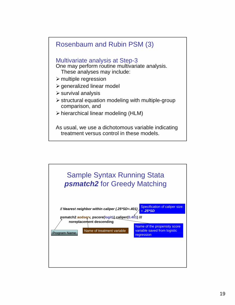
Rosenbaum and Rubin PSM (3)

Multivariate analysis at Step-3One may perform routine multivariate analysis.

These analyses may include:These analyses may include:multiple regression generalized linear modelsurvival analysisstructural equation modeling with multiple-group comparison andcomparison, and hierarchical linear modeling (HLM)

As usual, we use a dichotomous variable indicating treatment versus control in these models.

Sample Syntax Running Stata psmatch2 for Greedy Matching

// Nearest neighbor within caliper (.25*SD=.401)

psmatch2 aodserv, pscore(logit1) caliper(0.401) ///noreplacement descending

Program Name

Specification of caliper size:= .25*SD

Name of treatment variable Name of the propensity score variable saved from logistic

Program Name regression

20

Example of Greedy Matching (1)Research QuestionsThe association between parental substanceThe association between parental substance

abuse and child welfare system involvement is well-known but little understood. This study aims to address the following questions: Whether or not these children are living in a safethese children are living in a safe environment? Does substance abuse treatment for caregivers affect the risk of child maltreatment re-report?

Example of Greedy Matching (2)Data and Study Sample

A secondary analysis of the National Survey of y y yChild and Adolescent Well-Being (NSCAW) data.

It employed NSCAW of two waves: baseline information between October 1999 and December 2000, and the 18-months follow-up. , pThe sample for this study was limited to 2,758 children who lived at home (e.g., were not in foster care) and whose primary caregivers were female.

21

Example of Greedy Matching (3)Measures

The choice of explanatory variables (i.e., matching p y ( gvariables) in the logistic regression model is crucial. We chose these variables based on a review of substance abuse literature to determine what characteristics were associated with treatment receipt. We found that these characteristics fall into four categories: demographic characteristics; risk factors; prior receipt of substance abuse treatment; and need for substance abuse services.

Example of Greedy Matching (4)Analytic Plan:

“3 x 2 x 2 design” = 12 Matching Schemes: Threelogistic regression models (i e each specified alogistic regression models (i.e., each specified a different set of matching variables); Two matching algorithms (i.e., nearest neighbor within caliper and Mahalanobis), and Two matching specifications (i.e., for nearest neighbor we used two different specifications on caliper size, and for Mahalanobis we used one with and one without propensity score as a covariate to calculate the Mahalanobis metric distances). Outcome analysis: survival model using Kaplan-Meier estimator evaluating difference in the survivor curve.

22

Example of Greedy Matching (5)Findings:

Children of substance abuser service users appearabuser service users appear to live in an environment that elevates risk of maltreatment and warrants continued protective supervision.The analysis based on the original sample without 0.

250.

500.

751.

00

Sample Based on Matching Scheme 9 N=482

original sample without controlling for heterogeneity of service receipt masked the fact that substance abuse treatment may be a marker for greater risk.

0.00

0 5 10 15 20analysis time

aodserv = 0 aodserv = 1

Example of Greedy Matching (6)For more information about this example, see

Guo & Fraser, 2010, pp.175-186.Guo, S., Barth, R.P., & Gibbons, C. (2006). Propensity score matching strategies for evaluating substance abuse services for child welfare clients. Children and Youth Services Review 28: 357-383Barth, R.P., Gibbons, C., & Guo, S. (2006). Substance abuse treatment and the recurrence of maltreatment among caregivers with children living at home: A propensity score analysis. Journal of Substance Abuse Treatment 30: 93-104.

23

Example of Greedy Matching (7)Additional examples of child welfare research

employing greedy matching:Barth, R.P., Lee, C.K., Wildfire, J., & Guo, S. (2006). A comparison of the governmental costs of long-term foster care and adoption. Social Service Review 80(1): 127-158.Barth, R.P., Guo, S., McCrae, J. (2008). Propensity score matching strategies for evaluating the success of child and family service programs. Research on Social Work Practice 18, 212-222.Weigensberg, E.C.; Barth, R.P., Guo, S. (2009). Family group decision making: A propensity score analysis to evaluate child and family services at baseline and after 36-months. Children and Youth Services Review, 31, 383-390.

CCONTACT IINFORMATION

Ken DeCerchio, MSW, CAPProgram Director

Shenyang Guo, PhDProfessor of Social WorkProgram Director

Center for Children & Family FuturesPhone: (714) 505-3525Cell: (850) 459-3329E-mail: kdecerchio@cffutures.orgWebsite: www.ncsacw.samhsa.gov

Professor of Social WorkUniversity of North CarolinaPhone: (919) 843-2455Email: sguo@email.unc.edu

46

24

QUESTIONS AND DISCUSSION

47

THANK YOU!

PLEASE TAKE A BRIEFPLEASE TAKE A BRIEF MOMENT TO COMPLETE OUR

EVALUATION.

YOU WILL BE RE DIRECTEDYOU WILL BE RE-DIRECTED TO THE EVALUATION AFTER

EXITING THIS WEBINAR.48