How do households respond to income shocks?∗

Dirk Krueger

University of Pennsylvania, CEPR and NBER

Fabrizio Perri

University of Minnesota, Minneapolis FED, CEPR and NBER

August 2009

Abstract

Commonly used consumption/saving models have radically different implications for

households response to income shocks, ranging from the hands-to-mouth model, where

consumption bears all the adjustment, to the complete markets model, where wealth

bears all the adjustment. In this paper we use the Italian Survey of Household Income

and Wealth, which is the only available micro dataset that contains a panel on income,

consumption and wealth, to document how consumption and wealth co-move with short

run and long run income changes and to assess which model best captures this response.

We find that households who do not own real estate nor businesses change their con-

sumption and their wealth by about 23 and 17 cents, respectively, in response to a short

run 1 Euro change in after-tax labor income. For longer run income changes consump-

tion response becomes stronger and wealth response weaker. We show this response

to be quantitatively consistent with a permanent income model with quadratic utility

but not with a model in which households have CRRA utility and thus an income and

wealth-dependent precautionary saving motive. We finally show that for households

owning real estate or businesses, consumption response is weaker and wealth response

is much stronger, suggesting an important role for additional shocks, possibly correlated

with income shocks.

jel codes: d91, e21

key words: Consumption, Risk Sharing, Precautionary saving, Incomplete Markets

∗PRELIMINARY. We thank Ctirad Slavik for excellent research assistance, seminar participants at theUniversity of Minnesota, University of Pennsylvania, Cowles Foundation, St. Louis and Philadelphia FED,Arizona State, Carnegie Mellon, Penn State, Rochester, University of Virginia, Duke, SUNY Albany, ECB,Frankfurt, SAVE Conference in Deidesheim and the 2008 SED and NBER Summer Institute for many helpfulsuggestions and the NSF (under grant SES-0820494) for financial support.

1 Introduction

In micro-founded macro models households face one fundamental decision problem, namely

how to choose consumption and saving in the presence of both deterministic labor income

changes as well as labor income shocks. The feasible consumption-savings choices of house-

holds crucially depend on the menu of financial and real assets available to them. Existing

models differ starkly with respect to the assumptions regarding this menu. At one extreme,

in so-called hand-to-mouth consumer models financial asset are entirely absent and con-

sumption bears all the adjustment to income shocks. In the other extreme, the complete

markets model (the underlying abstraction of any representative agent macro model) envi-

sions a full set of state contingent assets that households can trade without binding short

sale constraints. In this model wealth bears all the adjustment to an income shock, and

consumption bears none. The assumptions the model builder makes about the structure of

financial markets are crucial not only for the positive predictions of the model (e.g. the joint

income-consumption dynamics, the response of the macro economy to shocks, the pricing of

financial assets) but also for normative policy analysis. The desirability of social insurance

policies (e.g. unemployment insurance, a redistributive tax code) depend crucially on how

well households can privately (self-) insure against idiosyncratic income shocks, which in

turn is determined by their access to and the sophistication of asset markets. Thus, it is

important to determine empirically what actual households do when they receive income

shocks, and to study which consumption-savings model provides the best approximation

to this observed behavior. The importance of the question has indeed generated a lot of

work on this issue but the conclusion of which model fits best actual household response is

still unclear. We conjecture that one reason for this is that most authors have focused on

consumption response to income shocks and have not explicitly analyzed wealth response,

mostly due to the lack of suitable data. This paper is, to the best of our knowledge, the

first attempt of evaluating models of household response to income shocks using data on

changes in income, consumption and wealth, both in the short and in the long run.

To carry out our analysis, we use a unique panel data set that contains detailed infor-

mation about household income, consumption and wealth, the Italian Survey of Household

Income and Wealth (SHIW) to document how various household choices (consumption of

nondurables and durables, capital income and wealth accumulation) change in response to

an income change. Our analysis documents co-movements, at the household level, of la-

bor income with other components of income, with various component of consumption and

wealth for the whole sample of households who have at least one member who is between the

1

age of 25 and 55 and is not retired. The analysis suggests that is useful to divide households

in two groups: households who do own businesses or real estate and households who do not.

We find that for households who do not own wealth nor real estate nondurable consumption

changes by about 23 cents in response to a short run (two years) 1 Euro change in after-

tax labor income, while financial wealth responds by about 17 cents. We also find that

in response to longer run (six years) income changes the consumption response becomes

stronger, while the wealth response becomes weaker. For households who own real estate

or businesses we find that the consumption response to income shocks is much smaller (in

the order of 5 cents to the dollar) while the wealth response is considerably larger.

We then explore whether various versions of a standard incomplete markets model can

account for this empirical evidence. We first evaluate the simplest variant of such a model,

a formalized version of the permanent income hypothesis, in which households can freely

borrow and save with a risk-free bond whose real return equals the subjective household

time discount rate, face no binding borrowing constraints, have quadratic utility and face

both purely transitory and purely permanent shocks. In that model one can derive the

consumption and wealth responses to an income shock analytically and show that they are

simple functions of the ratio between the variance of the transitory and the permanent

shock, as well as the share of the transitory shock that is due to measurement error. We

show that the co-movement between income, consumption and wealth changes both in the

short run and in the long run predicted by the model is consistent with that observed in the

data for non-business, non-real estate owners, if transitory shocks are an important source

of income changes and if measurement error in income is substantial. As we argue in the

paper, we believe that the relative magnitude of transitory income shocks and measurement

error required for the model to fit the data is plausible, and therefore we conclude that the

simple PIH model does remarkably well in explaining the observed consumption and wealth

responses in the short run.

We next show that, in the context of the standard incomplete markets model, the long

run wealth response to an income shock is particularly informative about the nature of the

precautionary savings motive. In models in which the size of precautionary saving motive

is independent of the income realization or the wealth level of the household (such as the

PIH or a model with CARA utility and nonbinding borrowing constraints1) the wealth1In the PIH model there is no precautionary saving at all. In a model with CARA utility, absent bor-

rowing constraints, households engage in precautionary saving, but the amount they save for precautionarymotives is independent of their income or wealth level, and the realization of their income shock. Thusthe PIH and the CARA utility version of the incomplete markets model have exactly the same predictionshow consumption responds to an income shock (and thus exactly the same predictions for the regressioncoefficients we estimate).

2

response to an income shock should be falling with the time horizon of an income change

(i.e. the wealth response to a 1 Euro income change over two years should be stronger

than the response to a 1 Euro income change over six years). In contrast, in versions

of the incomplete markets model in which households have CRRA utility (and/or face

borrowing constraints) we will show that the wealth response to an income shock should be

increasing with the time horizon. Therefore the empirical evidence that the wealth responses

to income shocks weakens with the time horizons suggests that the income and wealth

dependent precautionary savings motive implied by the CRRA model does not receive

empirical support from our Italian data. Instead, also along this dimension the empirical

findings are more consistent with the pure PIH.

We then analyze the wealth response to income shocks in more detail and document

that, or all components of wealth, the value of real assets (especially real estate and busi-

nesses) co-moves especially strongly with labor income shocks, for the whole sample of

households. We argue that a large part of this co-movement may be driven by a strong

correlation between labor income shocks and the prices of real estate (respectively, the value

of businesses), rather than reflect wealth accumulation behavior of households in response

to income shocks. This leads us to conclude that a simple model in which households only

face idiosyncratic income shocks, but not shocks to the value of their assets, might only be

a good approximation for households that do not own real estate or businesses, but not for

the entire sample households. This conclusion in turn motivates our sample selection in the

first part of the paper.

The paper is organized as follows. In the next section we briefly place our contribution

into the existing empirical and theoretical-quantitative literature. The data we use as well

as the empirical results we derive are discussed in section 3. In section 4 we present and

evaluate simple partial equilibrium versions of incomplete markets consumption-savings

models against the empirical facts documented in section 3. Section 5 presents further

evidence on the importance of adjustments in the value of real estate and business wealth

associated with labor income shocks, and section 6 concludes.

2 Related Literature

This paper builds on the large literature that has used household level data sets to evaluate

or formally test the empirical predictions of Friedman’s (1957) permanent income hypothesis

and related partial equilibrium incomplete markets models. Hall and Mishkin (1982) and

Altonji and Siow (1987) represent seminal contributions, and the early body of work is

3

discussed comprehensively in Deaton (1992). How strongly consumption responds to income

shocks of a given persistence is the central question of this literature.2

How strongly consumption responds to income shocks has also been estimated, for the

U.S., in the context of tests of perfect consumption insurance, see e.g. Mace (1991), or

Cochrane (1991). These tests do not need to distinguish between expected income changes

and income shocks, and between transitory and permanent shocks since all income fluctu-

ations ought to be smoothed and all shocks fully insured, according to the null hypothesis

of perfect consumption insurance.

Dynarski and Gruber (1997) and Krueger and Perri (2005, 2006) take a more agnostic

view and present the correlation between income and consumption changes as a set of

stylized facts that quantitative models ought to match. The spirit of our empirical analysis

is similar to these studies. For Italy, in a sequence of papers Jappelli and Pistaferri (2000,

2006, 2008a, 2008b) employ the SHIW data to study the dynamics of household income,

and the latter three the joint dynamics of household income and consumption.3

Recently Blundell et al. (2008) have constructed a consumption and income panel

by skillfully merging data from the CEX and the PSID, and used this panel to estimate

the extent to which households can insure consumption against transitory and permanent

income shocks. Kaplan and Violante (2008) evaluate whether a class of incomplete markets

models can rationalize the empirical estimates for consumption insurance that Blundell et

al. (2008) obtain.

Finally, Aaronson et al. (2008) investigate the consumption response to an increase in

the real wage in the U.S. Similar to our study they find that the adjustment in real estate

wealth is a crucial feature in their data, and they construct a model with housing wealth

to account for the facts.

3 Evidence

3.1 Data Description

The data set we use is the Survey of Household Income and Wealth (henceforth SHIW)

conducted by the Bank of Italy. The survey started in 1965 but before 1987 it did not contain

any panel dimension and did not contain complete wealth and consumption data. From 1987

on the SHIW has been conducted every two years (with the exception of the 1995 and 19982How strongly households’ consumption responds to predictable changes in income is the subject of studies

on excess sensitivity. The excess smoothness literature studies how strongly household consumption adjustsin response to permanent income shocks. See e.g. Luengo-Prado and Sorensen (2008).

3See Padula (2004) for another empirical study that uses the same Italian data.

4

surveys which were conducted 3 years apart) and it includes about 8000 households per year,

chosen to be representative of the whole Italian population. Also it has a panel structure

and a fraction of households in the sample is present in the survey for repeated years. This

data set is valuable and unique for our purposes as it contains panel information for many

categories of income, consumption and wealth for each household.4 The panel dimension

on income is particularly helpful for assessing the nature (i.e. permanent or temporary) of

income changes. The fact that the data contains, for the same household, panel information

on income, consumption and wealth is crucial for inferring how a given household adjusts its

consumption in response to an income change of a given type, and which and how various

components of wealth change in association with income fluctuations.5 Table A1 in the

appendix displays the total sample size of the data as well as the share of the households

in each wave of the SHIW that was present already in previous waves. We observe that

the panel dimension of the data set since 1989 is substantial and has grown over time, with

the fraction of all households in the 2006 wave already being present in previous waves

exceeding 50%.

Since the focus of this project is on the effects of earnings changes for households who

are active in the labor market we define an observation as a household who is in the survey

for at least two consecutive periods and whose head is between the age 25 and 55 and is not

retired in both periods. This leaves us with a sample of 12636 observations over the period

1987-2006.

3.2 Organization of the Data and Measurement

In order to organize our empirical findings we place them into the context of a sequential

budget constraint of a standard incomplete markets model in which the household can

self-insure by buying and selling a limited set of assets:

cnt + cdt + at+1 + et+1 = yt + pt + at + et + Tt, (1)4Jappelli and Pistaferri (2008) show that aggregate consumption and aggregate income from the SHIW

display growth rates that are very similar to the corresponding NIPA figures, suggesting that the coverageof the survey is comprehensive.

5The US consumer expenditure (CEX) survey has a panel dimension but the fact that it is short (onlytwo periods), that observation periods for income and consumption do not perfectly coincide (see Gervaisand Klein, 2006 for a treatment of this problem) and the fact that there is no panel dimension for wealthmakes it of limited use for our purposes. The US panel study on income dynamics (PSID) on the other handcontains a long panel for income but only has information on food consumption, and limited information onwealth, again making it hard to comprehensively assess the full impact of income shocks.

5

where cnt, cdt denote consumption expenditures on nondurables (including rent and imputed

rent for owner occupied housing) and durable consumption, respectively. at+1 and et+1

denote the values of the net asset position of financial and real wealth at the end of period

t, whereas yt measures after-tax labor income, Tt net private and public transfers, and pt

denote asset income, including income from financial assets (i.e. interests and dividends)

and income from real wealth (rental income), correspondingly. Financial wealth includes

liquid assets such as stocks and bonds while real wealth includes three types of less liquid

assets i.e. real estate, ownership shares of non incorporated business and valuables (i.e.

precious metals, art etc). Our Italian data is rich enough that we can measure all these

variables for our households in the sample.6 The first step of our empirical analysis is to

control for differences in family size across households by expressing all variables in adult

equivalent units by dividing each observation by the appropriate OECD equivalence scale.7

Table 1 below reports some basic summary statistics for our sample.

Table 1. Sample summary statistics

Average Level Annualized Growth

(1987) (2006) (1987-2006)

Age of head 41.5 44.6 0.4%

Household size 3.8 3.3 -0.7%

Labor income 8156 10646 1.4%

Asset income 1211 2690 4.3%

Transfers 285 563 3.6%

Non Durable consumption 5766 6858 0.9%

Durable consumption 860 888 0.2%

Real Wealth 25603 71366 5.5%

Financial Wealth 5124 9638 3.4%

Note: All variables except age and size, are per adult equivalent and in 2000 Euros

We then denote by ∆Nx = xt−xt−NN the annualized difference between an equivalized

variable x today and N periods ago and we obtain, setting N = 2 (with the exception of6For the exact variable definitions in the SHIW, please see Appendix A7This procedure has a minor impacts on the results. For labor income yt, for example, around 99% of the

cross-sectional variation of equivalized income growth is due to variation in the growth rate of raw income.

6

t t+1 t+2 t+3 time

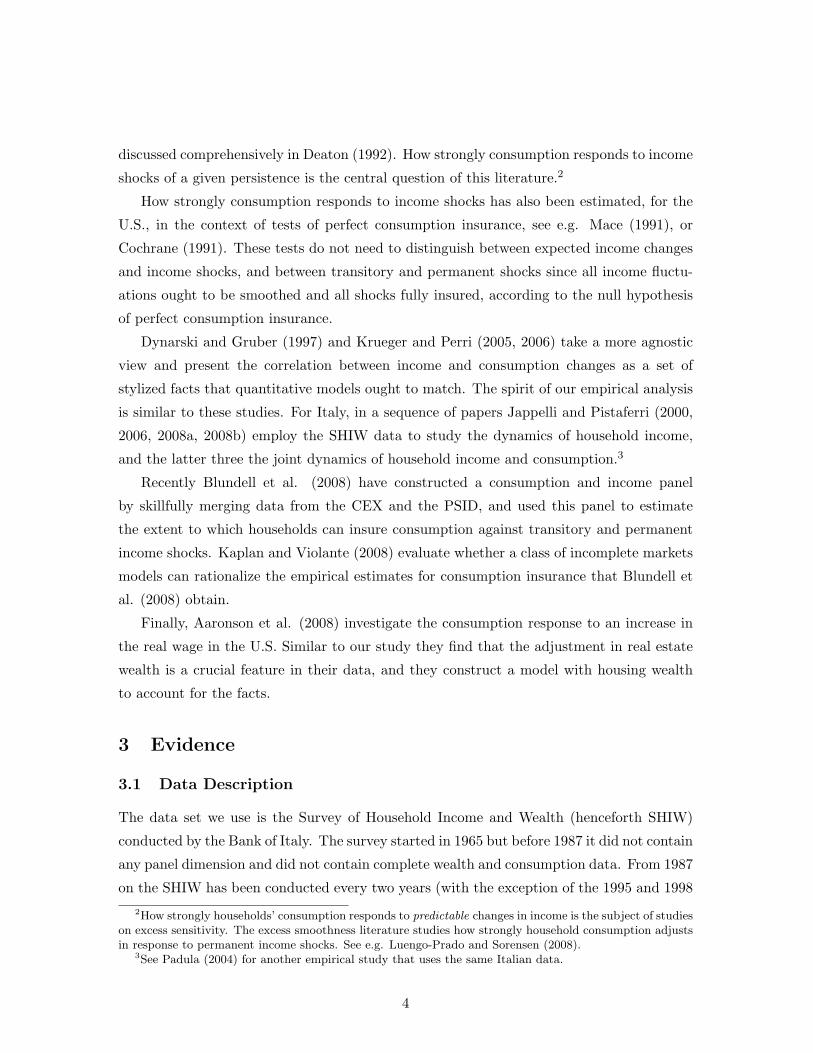
Observed: cnt, cdt, yt, Tt, pt cnt+2, cdt+2, yt+2, Tt+2, pt+2at+1, et+1 at+3, et+3

Not Observed: at, et at+2,et+2

Figure 1: Timeline in the SHIW

1998 where we set N = 3):

∆2cnt + ∆2cdt + ∆2at+1 + ∆2et+1

= ∆2yt + ∆2pt + ∆2retet + ∆2Tt

+∆2at + ∆2et (2)

Note that due to the biannual nature of our data set the last two terms ∆2at and ∆2et

cannot be observed in the data. This fact is clarified in figure 1 which shows the frequency

and exact timing with which different variables are observed in the SHIW data set.

The empirical question we want to answer now is how the observable differences in the

budget constraint co-move with changes in labor income ∆2yt. Since our main focus is on

income changes that are idiosyncratic and unpredicted (that is, on idiosyncratic income

shocks) we first attempt to purge the data from aggregate effects and predictable individual

changes by regressing each change on time dummies, on a quartic in the age of the head

of the household, on education and regional dummies, and on age-education interaction

dummies. Our empirical exercise is then carried out on the residuals from these first-stage

regressions.

7

0

.1

.2

.3

.4

.5

.6

.7

.8

.9

1P

erce

nt o

f hou

seho

lds

-.9 -.7 -.5 -.3 -.1 .1 .3 .5 .7 .9-1 -.8 -.6 -.4 -.2 0 .2 .4 .6 .8 1Growth rates in income

0

.1

.2

.3

.4

.5

.6

.7

.8

.9

1

Per

cent

of h

ouse

hold

s

-7 -5 -3 -1 1 3 5 7-8 -6 -4 -2 0 2 4 6 8Changes in income (Thousands of 2000 Euros)

Note: Income is real after tax labor + business per adult equivalent. Growth rates and changes are annualized

Figure 2: CDF of residual income variation

3.3 Empirical Results

In figure 2 we display the cumulative distribution function of observed residual annualized

labor income changes and log changes. The picture shows that a substantial fraction (about

20%) of households experience income changes that are larger than 2000 Euros (annualized,

per adult equivalent) or larger than 20% of their labor income.

In order to assess which are the households which are more subject to shocks in figure

3 we order households with respect to residual income changes, sort them into twenty

equally sized bins and for each bin we plot the fraction of households whose head is self-

employed. The figure shows clearly how self-employed households experience, on average,

larger absolute and relative changes.8

We fully acknowledge that a possibly large share of this observed variation may be due

to measurement error or to components that are predictable to the household but not to8Guiso et al. (2005) document that Italian firms provide substantial earnings insurance to its employees

against firm-specific shocks. The stark difference between the earnings shocks for employees and self employedin figure 3 could therefore partly be due to the fact that employees are partially insured by their firms againstidiosyncratic (to the fim or the worker) productivity shocks.

8

.1.2

.3.4

.5Fr

actio

n of

sel

f em

ploy

ed

-6000 -4000 -2000 0 2000 4000 6000Res. Labor income changes

.1.2

.3.4

.5Fr

actio

n of

sel

f em

ploy

ed

-.6 -.4 -.2 0 .2 .4 .6Res. Labor income log-changes

Figure 3: Income variation and self employment

9

­600

0­4

000

­200

00

2000

4000

6000

Inco

me 

and 

cons

umpt

ion 

chan

ges

­6000 ­4000 ­2000 0 2000 4000 6000Income changes (in 2000 Euros)

ND Consumption change Income change

Each bin contains 600 households

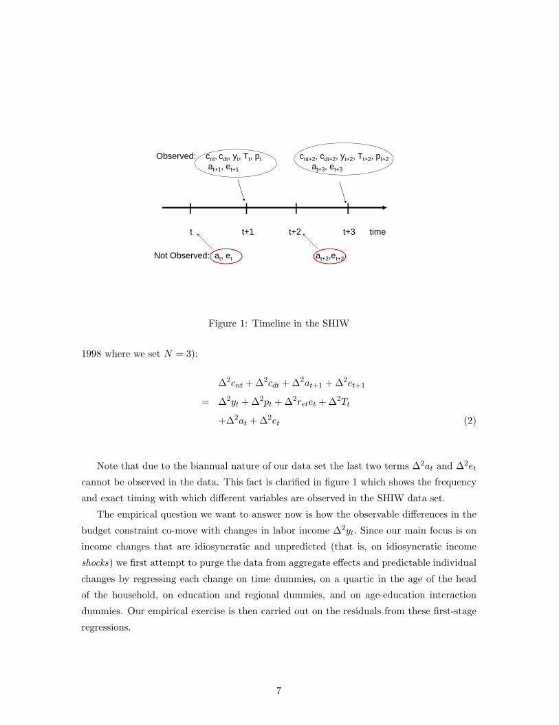
Figure 4: Changes in income and non durable consumption

us, and thus will address these issues explicitly when comparing the stylized facts from the

data to the predictions of the models we use to assess these facts.9

To visualize the co-movement of various components of the budget constraint with in-

come for each of the 20 bins of sorted income changes we compute the average change in

each observable component of the budget constraint and plot it against the corresponding

income change. Figures 4-6 contain the results of this exercise, for nondurable and durable

consumption, non-labor income components and all forms of household wealth.

From figure 4 we observe that nondurable consumption changes are positively correlated

with income shocks. In addition, that relationship appears to be fairly linear, although a

slightly larger response to income increases than to income declines can be observed. As

we make precise below in table 2, for the entire sample of households, on average a 1 Euro

increase (decline) in after-tax labor income is associated with about a 10 cents increase

(decline) in expenditures on nondurable consumption.9Altonji and Siow (1987), in their critique of Hall and Mishkin (1982) stress the potential quantitative

importance of measurement error in income changes or income growth for the type of regressions conducted

10

­60

00­4

000

­20

000

2000

4000

6000

Inc.

 and

 dur

. exp

. cha

nges

­6000 ­4000 ­2000 0 2000 4000 6000Income changes (2000 Euros)

Dur. expend. change Inc. change

Each bin contains 600 households

­60

00­4

000

­20

000

2000

4000

6000

Inc.

 and

 fina

nc. i

nc. c

hang

es

­6000 ­4000 ­2000 0 2000 4000 6000Income changes (2000 Euros)

Transfer change Inc. change

Each bin contains 300 households

­60

00­4

000

­20

000

2000

4000

6000

Inc.

 and

 pro

pt. i

nc. c

hang

es

­6000 ­4000 ­2000 0 2000 4000 6000Income changes (2000 Euros)

Propt. inc. change Inc. change

Each bin contains 600 households

­60

00­4

000

­20

000

2000

4000

6000

Inc.

 and

 fina

nc. i

nc. c

hang

es

­6000 ­4000 ­2000 0 2000 4000 6000Income changes (2000 Euros)

Financ. inc. change Inc. change

Each bin contains 600 households

Changes are annualized and in dev. from mean

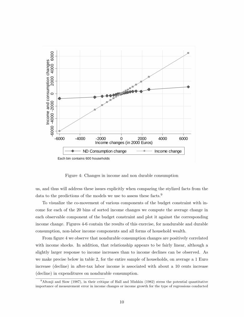
Figure 5: Changes in income and selected components of budget constraint

11

-180

00-1

2000

-600

00

6000

1200

018

000

Inc.

and

tot w

. cha

nges

-6000 -4000 -2000 0 2000 4000 6000Income changes (2000 Euros)

Tot. wealth change Inc. change

Each bin contains 600 households

-180

00-1

2000

-600

00

6000

1200

018

000

Inc.

and

fin.

w c

hang

es

-6000 -4000 -2000 0 2000 4000 6000Income changes (2000 Euros)

Fin. wealth Inc. change

Each bin contains 600 households

-180

00-1

2000

-600

00

6000

1200

018

000

Inc.

and

real

est

. cha

nges

-6000 -4000 -2000 0 2000 4000 6000Income changes (2000 Euros)

Real estate Inc. change

Each bin contains 600 households

-180

00-1

2000

-600

00

6000

1200

018

000

Inco

me

and

bus.

w. c

hang

es

-6000 -4000 -2000 0 2000 4000 6000Income changes (in 2000 Euros)

Business wealth Inc. change

Each bin contains 600 households

Changes are annualized and in dev. from mean

Figure 6: Changes in income and wealth components

In figure 5 we display the co-movement of after-tax labor income with other parts of

household income, in particular transfer income (the upper right panel), and capital income

from both real assets and financial assets (the lower two panels). The upper left panel

shows the change in consumption expenditures on consumer durables (mainly cars and

furniture) for each income change bin. We observe that changes in expenditures on consumer

durables co-move positively with income shocks but less so than changes in expenditures

on nondurables. Labor and capital income changes are, broadly speaking, uncorrelated

with each other. On the other hand, there is a visible, significant, but quantitatively small

negative co-movement between labor income changes and the change in net public and

private transfers received by households. This negative correlation is especially noticeable

for households with large income increases.

Figure 6 shows instead the co-movement of changes in various wealth components with

labor income and shows how total wealth and all its components (financial wealth, real

in this paper.

12

estate wealth and business wealth) strongly co-move with labor income.

In order to formally evaluate the magnitude of the average response of the various

components of the budget constraint to income changes we now run bivariate regressions of

the changes in the various component of the budget constraint on the changes in income:

results are reported in tables 2 and 3 below. Since the OLS estimates, in particular for the

wealth observations, may be influenced by a few large outliers that report large positive or

negative changes in wealth, we also report the median regression (MR) estimates resulting

from minimizing the sum of the absolute values of the residuals, rather than the sum of

squared residuals. By putting less weights on extreme observations MR estimates are more

robust to the influence of outliers.

Table 2. Co-movement with changes in labor income of:

∆cn ∆cd ∆T ∆TP ∆TO ∆p

βOLS9.8

(1.82)

6.5

(1.89)

-1.61

(0.40)

-3.8

(1.3)

2.4

(0.4)

1.77

(1.52)

R2 0.04 0.02 0.01 0.00 0.00 0.00

βMR

14.1

(0.27)

7.8

(0.6)

-0.08

(0.02)

-0.14

(0.01)

-0.04

(0.03)

1.78

(0.10)

R2 0.03 0.00 0.00 0.00 0.00 0.00

Obs. 12636 12636 12636 6216 6216 12636

Note: SE clustered at household level (for OLS) are in parenthesis

Results in table 2 quantitatively confirm the visual evidence from figures 4 and 5 that

changes in expenditures on consumer non durables ∆cn and in durables ∆cd are significantly

associated with changes in income but are much smaller than the income changes. On

average when income change by 1 Euro total consumption expenditures change by about 16

cents. The figure also shows that other sources of income are only weakly correlated with

labor income changes. This table also splits total net transfers T into transfers from family

and friends TF and other transfers TO (which includes pensions and arrears) indicates that

the former accounts for the majority of the (not very large) negative correlation between

labor income changes and changes in transfers.10 The adjustment of family transfers for a

Euro in lower labor income is in the order of 4 cents. The existence and negative correlation

with labor income changes of changes in family transfers may lend some qualitative support

to models that permit household to engage in more explicit insurance arrangements than the

simple self-insurance through asset trades that standard incomplete markets models envision10Note that the lower number of observation in the TF and TO regression is due to the fact that data on

disaggregated transfers are not available in the early survey years.

13

(e.g. models with private information or limited commitment). Note, however, that the

magnitude of these transfer changes and their correlation with labor income changes is

quantitatively small.

Table 3. Co-movement with changes in labor income of:

∆a ∆af ∆are ∆abw ∆av

βOLS252.2

(74.4)

10.6

(18.6)

30.2

(31.3)

221.7

(71.9)

4.4

(3.6)

R2 0.02 0.00 0.00 0.04 0.00

βMR

120.0

(3.34)

15.91

(0.61)

35.8

(1.96)

10.9

(0.65)

2.8

(0.16)

R2 0.01 0.00 0.00 0.00 0.00

Obs. 12636 12636 12636 12636 12636

Note: SE clustered at household level (for OLS) are in parenthesis

Results in table 3 confirm the findings from figure 6 that changes in labor income are

strongly associated with changes in wealth. The first column reports the result of regressing

residual changes in total wealth on residual changes in labor income while the subsequent

columns report the results using financial wealth (af ) real estate wealth (are) , business

wealth (abw) and valuables (av) Notice that results change significantly whether we use

OLS or MR suggesting that there are some households reporting very large changes in

wealth (in particular business wealth) which affect the OLS results. The upshot of the

table though is that, regardless of the regression method, on average a 1 Euro change in

labor income is associated with changes in wealth that are larger than 1 Euro. This result

suggest that a simple consumption/saving model in which a household is solely hit by income

shocks could never be consistent with this fact11 We conjecture that the main reason for

this result is the presence of shocks to the value of the wealth which are correlated with

the value of labor income. An example of this would be an entrepreneur that receives a

positive shock to the value of his business which at the same raise both her labor income

and her wealth. Another example would be a city specific shock which raise at the same

time labor income and wealth of the residents. So in order to isolate household response to

a ”pure” income shock we want to select households which do not have any members who

are self-employed/entrepreneur and who do not own real estate.11Note that this large change in the real value of assets is not in principle inconsistent with the budget

constraint. If income in period t − 1 (which we do not observe, due to the biannual structure of the dataset) were highly correlated with income change yt − yt−2 then the right hand side of the budget constraintcould change more than 1 Euro for each Euro in ∆y.In practice though, for empirically relevant process forincome, the correlation is not high enough to generate such a large response of wealth.

14

Table 4. Co-movements for selected sample

∆cn ∆cd ∆a

βOLS23

(2.2)

6.0

(2.2)

22.0

(12)

R2 0.02 0.00 0.00

βMR

23

(1.3)

1.3

(0.2)

17.1

(2.6)

R2 0.01 0.00 0.00

Obs. 2650 2650 2650

Note: SE clustered at household level (for OLS) are in parenthesis

The key result to notice from the table is that for this group nondurable consumption

co-moves significantly more with income and wealth significantly less. The consumption

response is in the order of 23 cents for the Euro, and the response of wealth 17 to 22

cents. In the next section we now assess whether, as a first check of theory, the standard

formalized version of the permanent income hypothesis in the spirit of Friedman (1957)

provides a reasonable approximation of the data for this selected group of households. This

analysis also provides some guidance along what dimension this basic model ought to be

extended to match the co-movements fact for the whole sample of households.

4 Theory

4.1 The Permanent Income Hypothesis

We now want to investigate whether versions of a standard incomplete markets model are

consistent with the facts displayed in the previous section. In this section we summarize

the empirical predictions of a model based on the permanent income hypothesis for the

question at hand, and evaluate to what extent the empirical evidence presented above is

consistent with this model. In the next section we then study a calibrated version of a

standard incomplete markets life cycle model with a precautionary savings motive.

Suppose that households have a quadratic period utility function, can freely borrow and

lend12 at a fixed interest rate r, discount the future at time discount factor β that satisfies12Of course a No-Ponzi condition is required to make the household decision problem have a solution.

15

β(1 + r) = 1 and faces an after-tax labor income process of the form

yt = y + zt + εt + γt

zt = zt−1 + ηt

where y is expected household income, εt ∼ N(0, σ2ε) is a transitory income shock, ηt ∼

N(0, σ2η) is a permanent income shock and γt ∼ N(0, σ2

γ) is classical measurement error in

income. The shocks (εt, ηt, γt) are assumed to be uncorrelated over time and across each

other. where (ε, η) are uncorrelated i.i.d. shocks with variances (σ2ε, σ

2η).

Aggregating across wealth components and focusing on nondurable consumption the

household faces a budget constraint of the form

ct + wt+1 = yt + (1 + r)wt

where wt = at + et is total and ct are expenditures on nondurable consumption, including

(imputed) rent for housing. We show in the appendix how a model that includes housing

explicitly can be reduced to the formulation studied in this section as long as there are

competitive rental markets, and the stock of housing can be adjusted without any frictions

or binding financing constraints. In addition, for the empirical implementation of this model

we include transfers Tt as part of after-tax labor income.

4.1.1 Empirical Predictions

As is well known, the realized changes in income, consumption and wealth of this model

are given by (see e.g. Deaton, 1992):

∆ct =r

1 + rεt + ηt

∆wt =εt

1 + r∆yt = ηt + ∆εt + ∆γt (3)

where ∆xt = xt − xt−1.

Equipped with these results we can now deduce the consumption and wealth responses

to income changes, as measured by the same bivariate regressions we ran for our Italian

data. First, since we have available a full panel and the survey is carried out only two

16

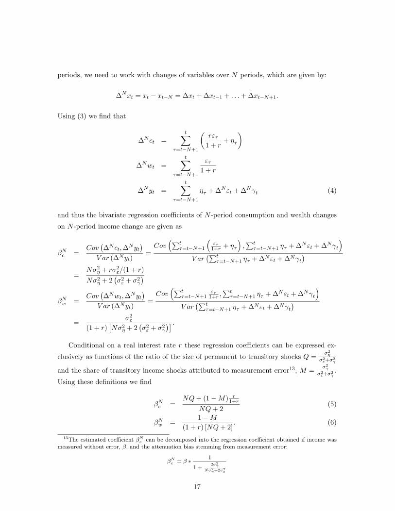
periods, we need to work with changes of variables over N periods, which are given by:

∆Nxt = xt − xt−N = ∆xt + ∆xt−1 + . . .+ ∆xt−N+1.

Using (3) we find that

∆Nct =t∑

τ=t−N+1

(rετ

1 + r+ ητ

)

∆Nwt =t∑

τ=t−N+1

ετ1 + r

∆Nyt =t∑

τ=t−N+1

ητ + ∆Nεt + ∆Nγt (4)

and thus the bivariate regression coefficients of N -period consumption and wealth changes

on N -period income change are given as

βNc =Cov

(∆Nct,∆Nyt

)V ar (∆Nyt)

=Cov

(∑tτ=t−N+1

(ετ

1+r + ητ

),∑t

τ=t−N+1 ητ + ∆Nεt + ∆Nγt

)V ar

(∑tτ=t−N+1 ητ + ∆Nεt + ∆Nγt

)=

Nσ2η + rσ2

ε/(1 + r)Nσ2

η + 2(σ2ε + σ2

γ

)βNw =

Cov(∆Nwt,∆Nyt

)V ar (∆Nyt)

=Cov

(∑tτ=t−N+1

ετ1+r ,

∑tτ=t−N+1 ητ + ∆Nεt + ∆Nγt

)V ar

(∑tτ=t−N+1 ητ + ∆Nεt + ∆Nγt

)=

σ2ε

(1 + r)[Nσ2

η + 2(σ2ε + σ2

γ

)] .Conditional on a real interest rate r these regression coefficients can be expressed ex-

clusively as functions of the ratio of the size of permanent to transitory shocks Q = σ2η

σ2ε+σ

2γ

and the share of transitory income shocks attributed to measurement error13, M = σ2γ

σ2ε+σ

2γ.

Using these definitions we find

βNc =NQ+ (1−M) r

1+r

NQ+ 2(5)

βNw =1−M

(1 + r) [NQ+ 2]. (6)

13The estimated coefficient βNc can be decomposed into the regression coefficient obtained if income wasmeasured without error, β, and the attenuation bias stemming from measurement error:

βNc = β ∗ 1

1 +2σ2γ

Nσ2η+2σ2

ε

17

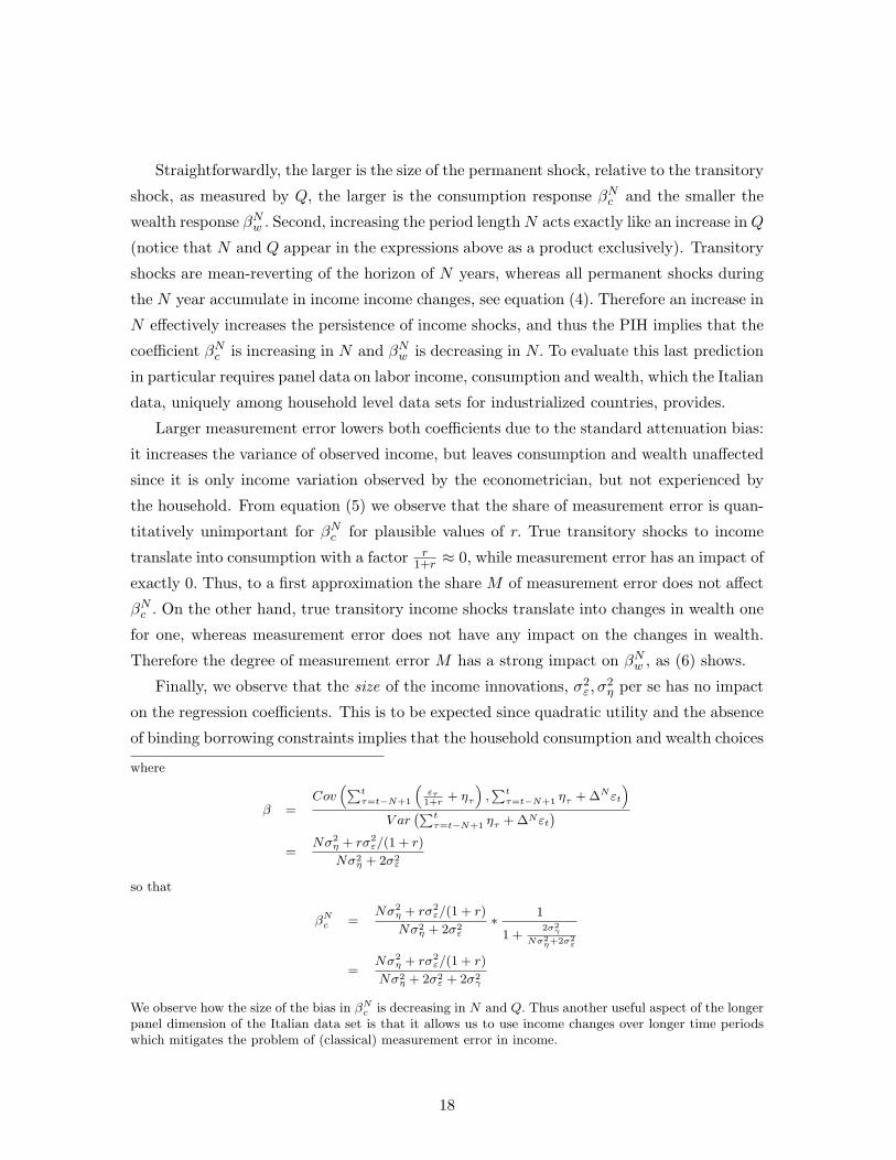
Straightforwardly, the larger is the size of the permanent shock, relative to the transitory

shock, as measured by Q, the larger is the consumption response βNc and the smaller the

wealth response βNw . Second, increasing the period lengthN acts exactly like an increase inQ

(notice that N and Q appear in the expressions above as a product exclusively). Transitory

shocks are mean-reverting of the horizon of N years, whereas all permanent shocks during

the N year accumulate in income income changes, see equation (4). Therefore an increase in

N effectively increases the persistence of income shocks, and thus the PIH implies that the

coefficient βNc is increasing in N and βNw is decreasing in N. To evaluate this last prediction

in particular requires panel data on labor income, consumption and wealth, which the Italian

data, uniquely among household level data sets for industrialized countries, provides.

Larger measurement error lowers both coefficients due to the standard attenuation bias:

it increases the variance of observed income, but leaves consumption and wealth unaffected

since it is only income variation observed by the econometrician, but not experienced by

the household. From equation (5) we observe that the share of measurement error is quan-

titatively unimportant for βNc for plausible values of r. True transitory shocks to income

translate into consumption with a factor r1+r ≈ 0, while measurement error has an impact of

exactly 0. Thus, to a first approximation the share M of measurement error does not affect

βNc . On the other hand, true transitory income shocks translate into changes in wealth one

for one, whereas measurement error does not have any impact on the changes in wealth.

Therefore the degree of measurement error M has a strong impact on βNw , as (6) shows.

Finally, we observe that the size of the income innovations, σ2ε, σ

2η per se has no impact

on the regression coefficients. This is to be expected since quadratic utility and the absence

of binding borrowing constraints implies that the household consumption and wealth choices

where

β =Cov

(∑tτ=t−N+1

(ετ1+r

+ ητ

),∑tτ=t−N+1 ητ + ∆Nεt

)V ar

(∑tτ=t−N+1 ητ + ∆Nεt

)=

Nσ2η + rσ2

ε/(1 + r)

Nσ2η + 2σ2

ε

so that

βNc =Nσ2

η + rσ2ε/(1 + r)

Nσ2η + 2σ2

ε

∗ 1

1 +2σ2γ

Nσ2η+2σ2

ε

=Nσ2

η + rσ2ε/(1 + r)

Nσ2η + 2σ2

ε + 2σ2γ

We observe how the size of the bias in βNc is decreasing in N and Q. Thus another useful aspect of the longerpanel dimension of the Italian data set is that it allows us to use income changes over longer time periodswhich mitigates the problem of (classical) measurement error in income.

18

obey certainty equivalence, and a precautionary saving motive is absent. In the next sub-

section we will evaluate how important the incorporation of a precautionary savings motive

is to rationalize the empirically observed co-movement of labor income, consumption and

wealth.

4.1.2 Evaluating the Empirical Predictions

We now ask whether for the sample of households that we identified in the empirical section

as most appropriately modeled by the PIH, households without business and real estate

wealth, the PIH is consistent with data. First, we let N = 2 and look at the minimal panel

dimension, which in turn contains the maximal number of households in the data. For

concreteness, we assume a real interest rate of 2%. Equations (5)-(6) show that the exact

value of the real interest rate affects the predicted values for (β2c , β

2w) only insignificantly.

We then ask what values of Q,M are needed to assure that the model predicts the same

regression coefficients as in the data.

Recall that the empirical regression results for the subsample under question delivered

a consumption response of β2c = 0.23 and a financial wealth response of β2

w = 0.17. Using

equations (5)-(6) we can determine which degree of income persistence Q and measurement

error M is required for the model to match the data perfectly along these two stylized

facts.14 The results are Q = 0.29 and M = 0.55. As discussion above indicates, the

empirical consumption response of 23 cents for each Euro implies that, for the PIH to be

consistent with this fact, that income shocks are largely driven by transitory shocks (since

permanent shocks imply a one-for-one consumption response). As discussed above, the size

of measurement error plays essentially no role for the consumption regression coefficient

in the model. Conditional on a value for Q determined from the consumption data, the

empirical wealth response then determines the required degree of measurement error.

With a choice of Q = 0.29 and M = 0.55 the PIH model matches the consumption and

financial wealth response to labor income shocks over a two year horizon by construction.

Thus this fact cannot be interpreted as a success of the model per se. However we would

like to point out that while it is hard quantify the amount of measurement error of income

in the data, the required value of income persistence Q = 0.29 is not implausible. With the14Given equations (5)-(6) we can simply solve for Q,M given the observed β2

c , β2w as

Q =β2c − rβ2

w

1− β2c + rβ2

w

M = 1− 2(1 + r)β2w

1− β2c + rβ2

w

19

panel dimension for labor income one can estimate Q directly from the data, conditional

on our assumption about the particular form of the income process. Jappelli and Pistaferri

(2008a,b) do exactly this for the Italian SHIW data and find Q ≈ 1/2, somewhat higher,

but in the range of the value required for the PIH to work well in a quantitative sense.1516

In the next section we investigate whether an extension of the current model that includes

a precautionary savings motive and thus implies that consumption responds to permanent

income shocks less than one for one (see Carroll, 2009) can rationalize the observed con-

sumption response of 23 cents with a persistence Q even more in line with the empirical

estimates by Jappelli and Pistaferri.

Before turning to the precautionary saving model we now more fully exploit the unique

panel dimension of the Italian data to evaluate the predictions of the PIH for income shocks

over longer time horizons, that is, for increasing N. An increase in N means that more

permanent shocks have accumulated, and that consumption should respond more strongly

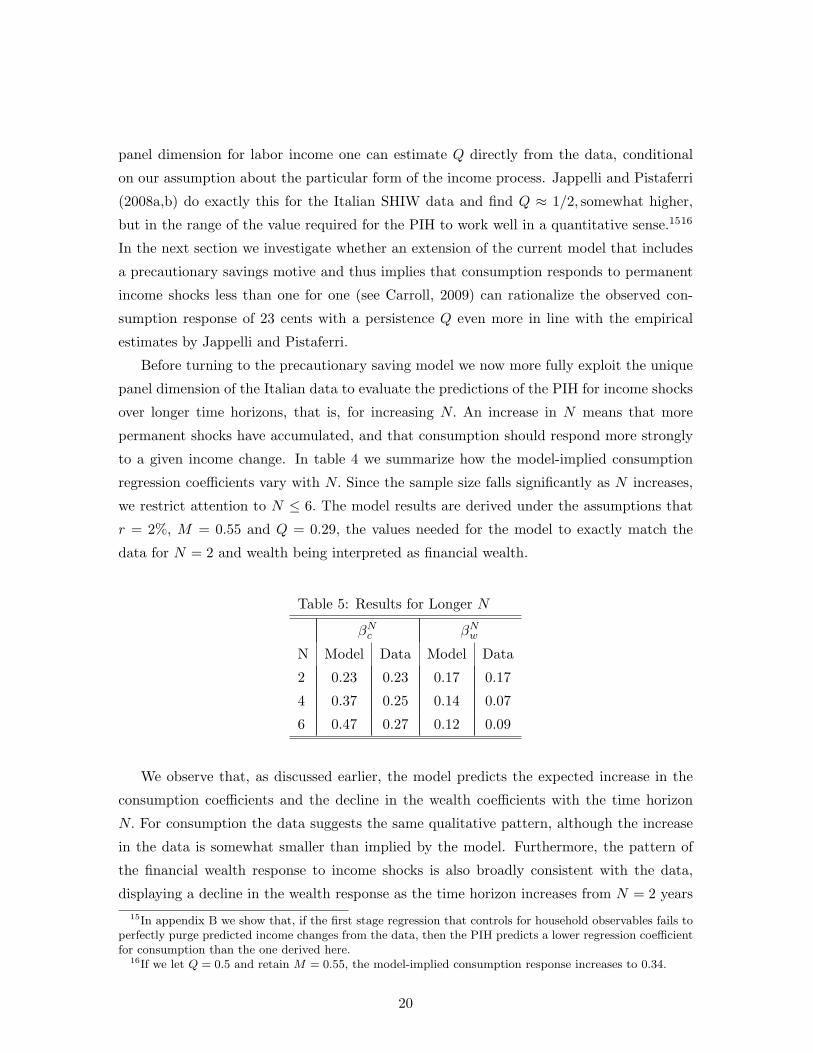
to a given income change. In table 4 we summarize how the model-implied consumption

regression coefficients vary with N. Since the sample size falls significantly as N increases,

we restrict attention to N ≤ 6. The model results are derived under the assumptions that

r = 2%, M = 0.55 and Q = 0.29, the values needed for the model to exactly match the

data for N = 2 and wealth being interpreted as financial wealth.

Table 5: Results for Longer N

βNc βNw

N Model Data Model Data

2 0.23 0.23 0.17 0.17

4 0.37 0.25 0.14 0.07

6 0.47 0.27 0.12 0.09

We observe that, as discussed earlier, the model predicts the expected increase in the

consumption coefficients and the decline in the wealth coefficients with the time horizon

N. For consumption the data suggests the same qualitative pattern, although the increase

in the data is somewhat smaller than implied by the model. Furthermore, the pattern of

the financial wealth response to income shocks is also broadly consistent with the data,

displaying a decline in the wealth response as the time horizon increases from N = 2 years15In appendix B we show that, if the first stage regression that controls for household observables fails to

perfectly purge predicted income changes from the data, then the PIH predicts a lower regression coefficientfor consumption than the one derived here.

16If we let Q = 0.5 and retain M = 0.55, the model-implied consumption response increases to 0.34.

20

to N = 6 years. Note that the findings for N = 4, 6 provide a true test for the model as all

model parameters have been chosen only with the data for N = 2 serving as targets.

To summarize, we conclude that the simple PIH model is successful in reproducing the

empirically observed dynamic consumption and financial wealth response to income shocks

of various durations. There are, however, two remaining empirical observations that this

model has trouble in rationalizing. First, the required degree of persistence of income shocks

seems at the high end of what the data suggests. Therefore in the next section we evaluate

whether introducing a precautionary savings motive into the model allows the model to

match the facts with the empirically estimated Q ≈ 0.5 by Jappelli and Pistaferri.

Second, the PIH cannot match the observed income-wealth correlations if wealth is

interpreted more broadly to include real estate wealth (and business wealth), an interpre-

tation that is mandated by a model that includes real estate explicitly (see appendix C).

We therefore, in section 5 investigate further what could explain the observed large positive

correlation between labor income shocks and real estate and business wealth.

4.2 A Precautionary Saving Model with CRRA Utility

The permanent income model abstracts from borrowing constraints and prudence in the

utility function (by assuming that u′′′(c) = 0). We now add these model elements that are

well-known to give rise to precautionary savings behavior and thus may have the potential

to reduce, quantitatively, the response of consumption to income shocks.

We envision a single household with monetary utility function u(c) = c1−σ

1−σ that faces

the tight borrowing constraint wt+1 ≥ 0. In addition in some versions of the model we cast

the household in a life-cycle context. Households live for 61 periods (from age 20 to 80

in real time). Prior to retirement at age 65, income of a household of age t is given by

yt = ytyt where the stochastic part of income y, in logs, is specified as a random walk plus

a transitory shock.

log(yt) = zt + εt

zt = zt−1 + ηt (7)

with εt ∼ N(−σ2ε

2 , σ2ε) and ηt ∼ N(−σ2

ε2 , σ

2η). The means of the innovations are chosen such

that E(y) = 1. After retirement households receive a constant fraction of their last pre-

retirement permanent income yt exp(zt) as pension. The income component yt denotes the

deterministic mean income at age t and follows the typical hump observed in the data.17

17In the infinite horizon of the model we set yt = 1 for all t.

21

The purpose of this section is to evaluate the potential of precautionary savings models

to deliver smaller consumption responses to income shocks. Rather than carrying out an

explicit calibration of the model we select parameter values that are plausible (relative to

the existing literature) and constitute a minimal deviation form the pure PIH discussed

above. With this objective in mind we select a CRRA of σ = 2 and choose ρ = r = 2%,

where ρ = 1β − 1 is the time discount rate of households. Jappelli and Pistaferri (2006,

table 3) estimate σ2ε = 0.0794 and σ2

η = 0.0267. Households start their life with w0 = 0 and

z−1 = 0.

In table 6 we summarize the consumption and in table 7 the wealth response to a labor

income shock over various time horizons, both in the data as well as in various models. The

column labeled ”PIH” is derived from the PIH model in which infinitely lived households

face an income process of the form in (7), with variances of permanent and transitory shocks

specified in the previous paragraph. For comparison we also include the results (labeled

“Analytical”) obtained with an income process specified in levels, in which case we have

provided the analytical expression of the regression coefficients in the previous section. The

fact that the results differ slightly from the previous section is due to the fact that Jappelli

and Pistaferri estimate a Q = 0.02670.0794 = 0.34 instead of the Q = 0.29 we had “calibrated”.

We observe that for all practical purposes it does not matter for the regression coefficients

in the PIH model whether the income process is specified in levels or in logs.

The column CRRA (T =∞) refers to results from the precautionary saving model with

infinite horizon, where we first solved the model for the optimal policy functions and then

simulated the model for 45 periods18, with the initial conditions specified in the previous

paragraph, and finally ran exactly the same regressions on the model-generated data as

we did for the real data. The last column shows results from the same procedure for the

precautionary saving model with an explicit life cycle income profile.

Table 6: Consumption Response

N Data PIH [Analytical] CRRA (T =∞) CRRA (T <∞)

2 0.23 0.25 [0.26] 0.13 0.19

4 0.25 0.40 [0.41] 0.21 0.30

6 0.27 0.50 [0.51] 0.26 0.38

18In this model consumption and wealth diverges to ∞ almost surely, therefore we cannot sample fromthe ergodic distribution, but rather simulate a large number of households for a short period of T = 45,starting always from the same initial condition.

22

We observe that, for consumption, the precautionary savings motive indeed reduces the

consumption response to an income shock (compare the third and forth column). Since

with finite horizon later in life transitory shocks are essentially permanent shocks as well,

the precautionary model with finite horizon implies larger consumption responses than the

corresponding precautionary model with infinite horizon. Both versions imply, as does the

PIH model and the data, that the consumption response increases with N. In addition, the

precautionary savings model’s predictions with T < ∞ are remarkably close to the data,

in a quantitative sense, despite the fact that it was not calibrated to achieve these targets.

The same is true, along the consumption dimension, for the basic version of the PIH, even if

the empirical estimates by Jappelli and Pistaferri for the income shock variances are used.

Table 7: Financial Wealth Response

N Data PIH [Analytical] CRRA (T =∞) CRRA (T <∞)

2 0.17 0.38 [0.37] 0.57 0.52

4 0.07 0.30 [0.29] 0.82 0.68

6 0.09 0.26 [0.25 1.14 0.88

Table 7 displays the corresponding wealth response. We observe that while the PIH

is qualitatively consistent with the decline of the wealth response with an increase in the

time horizon N (which we already documented in table 5).19 The CRRA models, on the

other hand, predict a substantial increase in the wealth response over longer time horizons,

qualitatively (and of course, quantitatively) at odds with the data. As N increases, the

persistence of the income shock increases, an effect that ought to reduce the wealth response

to income shocks with increasing N. On the other hand, in these models even permanent

shocks do not fully translate into corresponding consumption movements. Part of the

permanent income shocks are absorbed by wealth.20 Over longer periods more permanent

shocks accumulate, so the correlation between income and wealth changes increases with

the time horizon N. In models where permanent income shocks translate into consumption

one for one (as in the original PIH or the CARA model) wealth does not absorb any of

the permanent shocks. Thus in these models the wealth response to income shocks increase

with the time horizon as over longer time horizons the importance of permanent income19Quantitatively, the wealth response in the model is larger, for every value of N, than in the data. Adding

the appropriate degree of measurement error in income into the model would bring the model better in linewith the data along this dimension, as we already demonstrated in the previous section.

20Carroll (2009) demonstrates this result analytically and computationally in a model that is essentiallyidentical to the one we use here.

23

shocks increase, relative to transitory shocks (see the previous section). The fact that even

permanent shocks are partially insured in the CRRA model lets the wealth response to

income shocks rise with N, and also reduces the increase of the consumption response with

increased N, relative to the PIH model.21 22

We conclude that while the CRRA model with its partial insurance against permanent

shocks is helpful in reducing the overall consumption response to income shocks towards

the levels observed in the data, it is qualitatively inconsistent with the dynamic response

of financial wealth to income shocks. Therefore we conclude that, overall, the simple PIH

describes the consumption and wealth response to income shocks to a better, and very

reasonable degree, at least for households without real estate and business wealth. It remains

to be explored, however, what drives the large observed co-movement between income shocks

and real estate and business wealth observed in the data. We turn to this question next.

5 What Drives the Co-Movement between Income Shocks

and Real Estate and Business Wealth?

5.1 Real Estate Wealth

In Italy real estate is the predominant form of wealth held by private households. The

median wealth household in 2006 owned about 140,000 Euro worth of real estate, relative

to financial wealth of about 7000 Euro. As a point of comparison, median annual household

income amounted to about 26,000 Euro. Mortgage debt, on the other hand is not very

prevalent. Despite substantial increases in the last years the mortgagee debt to disposable

income ratio is a mere 20%. Consequently, real estate is by far the most important compo-

nent of total net worth of the median household. With 69% the home ownership rate is high

and comparable to that of the U.S. As a further indicator of the importance of real estate

wealth in a typical households’ portfolio, note that about 30% of all Italian households won

more than one property, with the average number of properties being owned equal to 1.44

(the median number is 1, though). It is therefore not entirely surprising that adjustments

in the real value of real estate may play an important role in a households’ response to an

income shock.21Table 6 shows that the difference in the consumption response between N = 2 and N = 6 is 0.25 in the

PIH model, but only 0.13-0.18 in the CRRA model that implies partial self-insurance against permanentshocks.

22The degree of prudence, as measured by σ, impacts the results quantitatively, but not qualitatively.Ceteris paribus, the larger is σ (the more prudent households are), the smaller is the consumption responseand the larger is the wealth response. Furthermore, the consumption response increases more slowly withN the larger is σ, and the wealth response increases more rapidly.

24

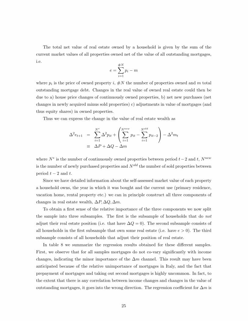
The total net value of real estate owned by a household is given by the sum of the

current market values of all properties owned net of the value of all outstanding mortgages,

i.e.

e =#N∑i=1

pi −m

where pi is the price of owned property i, #N the number of properties owned and m total

outstanding mortgage debt. Changes in the real value of owned real estate could then be

due to a) house price changes of continuously owned properties, b) net new purchases (net

changes in newly acquired minus sold properties) c) adjustments in value of mortgages (and

thus equity shares) in owned properties.

Thus we can express the change in the value of real estate wealth as

∆2et+1 =N∗∑i=1

∆2pit +

Nnew∑i=1

pit −Nold∑i=1

pit−2

−∆2mt

≡ ∆P + ∆Q−∆m

where N∗ is the number of continuously owned properties between period t−2 and t, Nnew

is the number of newly purchased properties and Nold the number of sold properties between

period t− 2 and t.

Since we have detailed information about the self-assessed market value of each property

a household owns, the year in which it was bought and the current use (primary residence,

vacation home, rental property etc.) we can in principle construct all three components of

changes in real estate wealth, ∆P,∆Q,∆m.

To obtain a first sense of the relative importance of the three components we now split

the sample into three subsamples. The first is the subsample of households that do not

adjust their real estate position (i.e. that have ∆Q = 0). The second subsample consists of

all households in the first subsample that own some real estate (i.e. have e > 0). The third

subsample consists of all households that adjust their position of real estate.

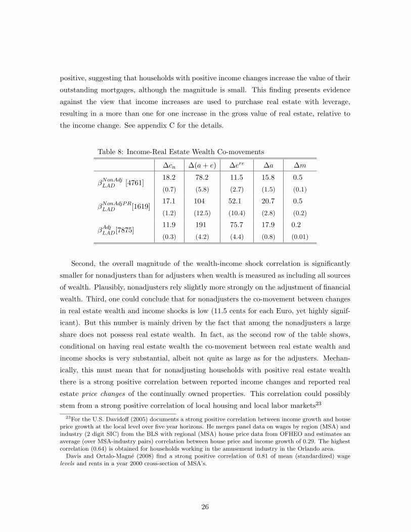
In table 8 we summarize the regression results obtained for these different samples.

First, we observe that for all samples mortgages do not co-vary significantly with income

changes, indicating the minor importance of the ∆m channel. This result may have been

anticipated because of the relative unimportance of mortgages in Italy, and the fact that

prepayment of mortgages and taking out second mortgages is highly uncommon. In fact, to

the extent that there is any correlation between income changes and changes in the value of

outstanding mortgages, it goes into the wrong direction. The regression coefficient for ∆m is

25

positive, suggesting that households with positive income changes increase the value of their

outstanding mortgages, although the magnitude is small. This finding presents evidence

against the view that income increases are used to purchase real estate with leverage,

resulting in a more than one for one increase in the gross value of real estate, relative to

the income change. See appendix C for the details.

Table 8: Income-Real Estate Wealth Co-movements

∆cn ∆(a+ e) ∆ere ∆a ∆m

βNonAdjLAD [4761]18.2

(0.7)

78.2

(5.8)

11.5

(2.7)

15.8

(1.5)

0.5

(0.1)

βNonAdjPRLAD [1619]17.1

(1.2)

104

(12.5)

52.1

(10.4)

20.7

(2.8)

0.5

(0.2)

βAdjLAD[7875]11.9

(0.3)

191

(4.2)

75.7

(4.4)

17.9

(0.8)

0.2

(0.01)

Second, the overall magnitude of the wealth-income shock correlation is significantly

smaller for nonadjusters than for adjusters when wealth is measured as including all sources

of wealth. Plausibly, nonadjusters rely slightly more strongly on the adjustment of financial

wealth. Third, one could conclude that for nonadjusters the co-movement between changes

in real estate wealth and income shocks is low (11.5 cents for each Euro, yet highly signif-

icant). But this number is mainly driven by the fact that among the nonadjusters a large

share does not possess real estate wealth. In fact, as the second row of the table shows,

conditional on having real estate wealth the co-movement between real estate wealth and

income shocks is very substantial, albeit not quite as large as for the adjusters. Mechan-

ically, this must mean that for nonadjusting households with positive real estate wealth

there is a strong positive correlation between reported income changes and reported real

estate price changes of the continually owned properties. This correlation could possibly

stem from a strong positive correlation of local housing and local labor markets23

23For the U.S. Davidoff (2005) documents a strong positive correlation between income growth and houseprice growth at the local level over five year horizons. He merges panel data on wages by region (MSA) andindustry (2 digit SIC) from the BLS with regional (MSA) house price data from OFHEO and estimates anaverage (over MSA-industry pairs) correlation between house price and income growth of 0.29. The highestcorrelation (0.64) is obtained for households working in the amusement industry in the Orlando area.

Davis and Ortalo-Magne (2008) find a strong positive correlation of 0.81 of mean (standardized) wagelevels and rents in a year 2000 cross-section of MSA’s.

26

5.2 The Role of Self-Employment

Households in which the household head is self-employed constitute a significant share of

households with the largest changes in labor income, suggesting that these households face

substantially more income risk. It is therefore instructive to investigate whether and to

what extent the consumption and wealth response of this group differs from the overall

sample. In table 9 we split the sample into self-employed households and their complement.

Table 9: The Role of Self-Employment

∆cn ∆(a+ e) ∆ere ∆ebw ∆a

βselfLAD [2613]5.7

(0.4)

148.2

(6.1)

20.9

(3.5)

17.8

(1.0)

15.8

(0.8)

βempLAD [10023]20.5

(0.4)

117.2

(5.9)

44.8

(3.2)

9.3

(1.3)

18.5

(1.2)

We observe that self-employed households have significantly lower consumption and

higher wealth responses than other households, where the wealth response is mainly driven

by the strong positive co-movement between labor income and business wealth. As with

real estate wealth, one plausible explanation is that shocks to labor income are positively

correlated with the value of the business wealth the entrepreneur owns, without necessarily

suggesting an active adjustment of the household in response to labor income shocks.

6 Conclusion

How do households respond to an income shock? In this paper we presented evidence that

Italian households surveyed in the SHIW adjust nondurable consumption by 23 cents for

each Euro and financial wealth by 17 cents. These observations are consistent with the

permanent income hypothesis if most income shocks are transitory in nature. We also

documented a strong positive correlation between labor income shocks and adjustments in

the value of real estate and business wealth. These findings suggest that shocks other than

labor income shocks are important in shaping household economic decisions, and that these

shocks (such as shocks to local house prices and businesses) might be strongly correlated

with labor income shocks faced by households. Future research has to address in more detail

the forces behind this large correlation. It also has to investigate whether the findings in this

paper can be generalized to other industrialized countries, a task that is complicated by the

lack of appropriate panel data elsewhere.24 It finally has to provide a uniform consumption-24The construction of panel consumption data from panel income data with minimal consumption content

and cross-sectional consumption data, as in Blundell et al. (2008) may present an alternative to the use of

27

savings model that incorporates these shocks, and endogenizes the housing adjustment and

business ownership decision.

References

[1] Aaronson, D. S. Agarwal and E. French (2008), “The Consumption Response to a

Minimum Wage Increase,” Chicago FED Working paper 2007-23.

[2] Altonji, J. and A. Siow (1987), “Testing the Response of Consumption to Income

Changes with (Noisy) Panel ,” Quarterly Journal of Economics, 102, 293-328.

[3] Banca d’Italia (2008), Supplements to the Statistical Bulletin Sample Surveys: House-

hold Income and Wealth in 2006, Rome.

[4] Blundell, R., L. Pistaferri and I. Preston (2008), “Consumption Inequality and Partial

Insurance,” forthcoming, American Economic Review.

[5] Campbell, J. and Z. Hercowitz (2006), “Welfare Implications of the Transition to High

Household Debt,” Working paper 2006-26, Federal Reserve Bank of Chicago.

[6] Carroll, C. (2009), “Precautionary Saving and the Marginal Propensity to Consume

out of Permanent Income, Journal of Monetary Economics, forthcoming.

[7] Cochrane, J. (1991), “A Simple Test of Consumption Insurance,” Journal of Political

Economy, 99, 957-976.

[8] Davidoff, T. (2005), “Labor Income, Housing Prices and Homeownership,” Working

Paper, UC Berkeley.

[9] Davis, M. and F. Ortalo-Magne (2008), “Household Expenditures, Wages, Rents,”

Working Paper, University of Wisconsin.

[10] Deaton, A. (1992), Understanding Consumption, Clarendon Press, Oxford.

[11] Dynarski, S. and J. Gruber (1997), “Can Families Smooth Variable Earnings?,” Brook-

ings Papers on Economic Activity, 229-284.

[12] Fernandez-Villaverde, J. and D. Krueger (2002), “Consumption and Saving over the

Life Cycle: How Important are Consumer Durables?” Proceedings of the 2002 North

American Summer Meetings of the Econometric Society: Macroeconomic Theory.

a full panel.

28

[13] Friedman, M. (1957), A Theory of the Consumption Function, Princeton University

Press.

[14] Gervais, M. and P. Klein (2006), “Measuring Consumption Smoothing in CEX Data,”

Working Paper, University of Western Ontario.

[15] Guiso, L., L. Pistaferri and F. Schivardi (2005), “Insurance within the Firm,” Journal

of Political Economy, 113, 1054-1087.

[16] Hall. R and F. Mishkin (1982), “The Sensitivity of Consumption to Transitory Income:

Estimates from Panel Data on Households,” Econometrica, 50, 461-481.

[17] Hansen, G. (1993), “The Cyclical and Secular Behavior of the Labor Input: Comparing

Efficiency Units and Hours Worked,” Journal of Applied Econometrics 8, 71-80.

[18] Jappelli T. and L. Pistaferri (2000a), “Using Subjective Income Expectations to Test for

Excess Sensitivity of Consumption to Predicted Income Growth,” European Economic

Review, 44, 337-358.

[19] Jappelli T. and L. Pistaferri (2000b), “The dynamics of household wealth accumulation

in Italy,”Fiscal Studies, 21(2), 269-295

[20] Jappelli T. and L. Pistaferri (2006), “Intertemporal Choice and Consumption Mobil-

ity,” Journal of the European Economic Association, 4, 75-115.

[21] Jappelli T. and L. Pistaferri (2008a), “Consumption and Income Inequality in Italy,”

Working Paper, Stanford University.

[22] Jappelli T. and L. Pistaferri (2008b), “Financial Integration and Consumption Smooth-

ing,” Working Paper, Stanford University.

[23] Kaplan, G. and G. Violante (2008), “How Much Insurance in Bewley Models?,” Work-

ing Paper, New York University.

[24] Krueger, D. and F. Perri (2005), “Understanding Consumption Smoothing: Evidence

from the US Consumer Expenditure Survey,” Journal of the European Economic As-

sociation Papers and Proceedings, 3, 340-349.

[25] Krueger, D. and F. Perri (2006), “Does Income Inequality Lead to Consumption In-

equality? Evidence and Theory,” Review of Economic Studies, 73, 163-193.

29

[26] Luengo-Prado, M. and B. Sorensen (2008), “What Can Explain Excess Smoothness

and Sensitivity of State-Level Consumption?,” Review of Economics and Statistics, 90,

65-80.

[27] Mace, B. (1991), “Full Insurance in the Presence of Aggregate Uncertainty,” Journal

of Political Economy, 99, 928-56.

[28] Padula, M. (2004), “Consumer Durables and the Marginal Propensity to Consume out

of Permanent Income Shocks,” Research in Economics 58, 319-341.

[29] Shin, D. and G. Solon (2008), “Trends in Men’s Earnings Volatility: What does the

Panel Study of Income Dynamics Show?,” NBER Working paper 14075.

30

A Variable Definitions

Nondurable consumption cnt is defined as all household expenditures during a year, minus

expenditures on transportation equipment (cars, bikes etc.), valuables (such as art, jewelry,

antiques), household equipment (such as furniture, rugs, TV’s, cell phones and other elec-

tronics), expenditure for home improvement, insurance premia and contribution to pension

funds. It includes rent paid by renters and imputed rent of home owners on all properties

that are not rented out. Imputed rent also appears as income from real assets in retet on the

right hand side of the budget constraint. Expenditures on durables cdt include expenditures

for transportation equipment, valuables and household equipment, all as defined above.

Labor income yt is measured after taxes and includes fringe benefits received by employ-

ees and business income by entrepreneurs. Transfers Tt include both transfer payments from

the government (such as unemployment benefits) as well as gifts, loans and other transfers

between private households.

Financial assets at+1 add bank deposits, stock and bond holdings and other direct hold-

ings of financial assets (including assets held in private pension funds), net of outstanding

debt. It does not include the value of entitlements to government pension payments. The

net income from financial assets (interest payments, dividends etc.) forms financial income

ratat. Finally, real assets et+1 include the value of real estate property, the value of valuables

(as defined above) and the net value of ownership in private businesses and partnerships.

Income from real assets, retet, consists mainly of rent (both actual and imputed) received

from owned real estate.

B Predictable Income Changes

To the extent that our first stage regression that conditions the data on observables such

as age, education etc. has failed to capture all predictable movements in income, the

empirical estimates may partially reflect the consumption response to predictable income

changes.25 The PIH model of course implies that consumption should not respond to

predictable changes in income at all. Denoting the predictable part of income by yt the

model now implies, for an income process

yt = yt + zt + εt + γt

zt = zt−1 + ηt

25On the other hand, It is possible that some of the variation the first stage regression picks up may havebeen predicted by the econometrician, but not by the household itself.

31

the model solution

∆yt = ηt + ∆yt + ∆εt + ∆γt

∆ct =r

1 + rεt + ηt

∆at+1 =εt

1 + r− 1

1 + r

∞∑s=1

∆yt+s(1 + r)s−1

.

N-period changes are therefore given by

∆Nct =t∑

τ=t−N+1

(rετ

1 + r+ ητ

)

∆Nyt =t∑

τ=t−N+1

ητ + ∆N yt + ∆Nεt + ∆Nγt

∆Nat+1 =t∑

τ=t−N+1

ετ1 + r

− 11 + r

∞∑s=1

∆N yt+s(1 + r)s−1

and the regression coefficients implied by the model now read as

βNc =Nσ2

η + rσ2ε/(1 + r)

Nσ2η + 2

(σ2ε + σ2

γ

)+ V ar (∆N yt)

βNw =−∑∞

s=1

Cov(∆N yt,∆N yt+s)(1+r)s + σ2

ε/(1 + r)

Nσ2η + 2

(σ2ε + σ2

γ

)+ V ar (∆N yt)

Thus the consumption response to income shocks goes down in presence of predicted

income changes, the extent to which is determined by how large the cross-sectional variance

in the N -period change in the predictable component of income is, relative to the variance

of the permanent and transitory income shocks. Note that the wealth response to income

changes now depends also crucially on the covariance of current and future predicted income

changes.

C Housing in the Standard Incomplete Markets Model

We now introduce housing explicitly into the standard incomplete markets model. We

first model the housing choice of households without any frictions in the adjustment of

real estate position and no explicit borrowing constraints.26 Also, households have access26Of course an appropriate no-Ponzi condition has to be imposed to make the household problem have a

solution.

32

to a competitive rental market where housing services st can be rented for a rental price

Rt per unit of house. Households buy real estate ht+1 at price per unit of pt, as well as

nondurable consumption cnt and financial assets at+1. Houses depreciate at rate δ. The

household decision problem is then given by

max{cnt,st,at+1,ht+1}

E0

∑t

βtv(cnt, st)

cnt + at+1 +Rtst + ptht+1 = yt + (1 + rt)at + pt(1− δ)ht +Rtht (8)

where v(cnt, st) gives the period utility from consuming nondurables cnt and housing ser-

vices st.

C.1 Analysis

It is straightforward to show that this household problem can be solved in three stages. In

the first stage the intratemporal consumption allocation problem between nondurables and

housing services is solved

maxcnt,st

v(cnt, st)

cnt +Rtst = ct

where ct is the expenditure on housing services. The solution characterized by the two

equations

vs(cnt, st)vcn(cnt, st)

= Rt

cnt +Rtst = ct

Define the indirect utility function resulting from this maximization problem as

u(ct;Rt) = v(cnt(ct, Rt), st(ct, Rt))

This is the period utility function used in the main text.

In a second stage the household decides how to split its savings between financial and

real assets. Without any frictions in the real estate market (or the financial asset market,

for that matter) a simple no-arbitrage argument implies that the rental price and the price

33

of real estate have to satisfy the condition.

Rt+1 = pt

[(1 + rt+1)− pt+1(1− δ)

pt

]Under this condition one can consolidate both assets into one

wt+1 = at+1 + ptht+1.

Exploiting the outcome of steps i) and ii) the intertemporal household problem then

reads as

max{ct,wt+1}

E0

∑t

βtu(ct;Rt)

ct + wt+1 = yt + (1 + rt)wt

where consumption expenditures and wealth are measured as

ct = cnt +Rtst

wt+1 = at+1 + ptht+1

= at+1 + et+1.

As long as ct and wt are measured empirically consistent with the theory, the analysis

can proceed as in the main text, without explicit consideration of the households’ housing

choice.

C.2 Adding Financing Constraints

Suppose the household can only finance a fraction 1−γ of the value of real estate purchased

in the current period,

at+1 ≥ −(1− γ)ptht+1.

The effect of such a constraint on the dynamics of the stock of real estate was studied, among

others, by Fernandez-Villaverde and Krueger (2002), Campbell and Hercowitz (2006) and

Aaronson et al. (2008). The presence of such a constraint may significantly alter the

response of housing wealth to a change in income. Suppose that households find it optimal

to be at the constraint in period t, then at+1 = −(1 − γ)ptht+1. Substituting this into the

34

budget constraint (8) yields

ct + γptht+1 = yt + (1 + rt)at + pt(1− δ)ht +Rtht.

Therefore if households are constrained in periods t− 1 and t we have

∆ct∆yt

+γ∆ptht+1

∆yt= 1.

It is straightforward to observe ∆ptht+1

∆yt> 1, that is expenditures on nondurables and net

new housing can exceed the income change since households can leverage home purchases.

But also note that this implies that

∆at+1

∆yt= −(1− γ)

∆ptht+1

∆yt

and thus one would expect large adjustments in the value of mortgages (or other financial

debt), too. This is not what the empirical analysis in section 5 of the main text reveals.

C.3 Adding Prohibitive Transaction Costs

Now imagine a household with current size of housing stock h that will never move, perhaps

because of prohibitively high transaction costs. Also assume that the households lives in

her own home, and does not rent out part of the home. Furthermore assume that the

depreciation rate on houses is δ = 0. Let the service flow from the owner-occupied house

h be given by s = φ(h), where φ is an arbitrary function. Then the household problem

(absent financing constraints) reads as

max{cnt,at+1}

E0

∑t

βtv(cnt, s)

cnt + at+1 + pt(ht+1 − ht) = yt + (1 + rt)at

and since by assumption ht+1 = ht, the budget constraint reads as

cnt + at+1 = yt + (1 + rt)at.

Evidently, the household does not care at all about changes in house prices. As long as the

utility function is additively separable in cn and s or satisfies

v(cnt, s) = g(s)u(cn) = g(φ(h))u(cn),

35

since h is constant by assumption the presence of housing services simply represents an

affine transformation of the period utility function that leaves nondurable consumption

choice behavior unaffected. Thus under these assumption we can proceed with our analysis

of the PIH or the more elaborate precautionary saving model as if housing wealth and

services are not present in the model.

With a nonzero depreciation rate δ > 0, house price changes affect measured disposable

labor income yt = yt − ptδh, but the model-implied map between the adjusted income

measure and nondurable consumption and financial wealth remains unaffected.

36