This paper presents preliminary fi ndings and is being distributed to economists and other interested readers solely to stimulate discussion and elicit comments. The views expressed in this paper are those of the authors and are not necessarily refl ective of views at the Federal Reserve Bank of New York or the Federal Reserve System. Any errors or omissions are the responsibility of the authors.

Federal Reserve Bank of New YorkStaff Reports

Staff Report No. 516September 2011

Revised January 2013

Matthew WiswallBasit Zafar

How Do College Students Respondto Public Information about Earnings?

REPORTS

FRBNY

Staff

Wiswall: Arizona State University, Department of Economics (e-mail: matt.wiswall@gmail.com). Zafar: Federal Reserve Bank of New York (e-mail: basit.zafar@ny.frb.org). This paper was originally issued as “Belief Updating among College Students: Evidence from Experimental Variation in Information.” The authors thank the NYU Center for Experimental Social Sciences for assistance conducting the information survey and experiment and participants at a Federal Reserve Bank of New York seminar and the NYU Experimental Economics Working Group. Da Lin and Scott Nelson provided outstanding research assistance. The views expressed in this paper are those of the authors and do not necessarily refl ect the position of the Federal Reserve Bank of New York or the Federal Reserve System.

Abstract

This paper investigates how college students update their future earnings beliefs using a unique “information” experiment: We provide college students true information about the population distribution of earnings, and observe how this information causes them to update their future earnings beliefs. We show that college students are substantially misinformed about population earnings, logically revise their self-earnings beliefs, and have larger revisions when the information is more specifi c and is “good” news. We classify the updating behaviors observed and fi nd that the majority of students are non-Bayesian updaters. While the average welfare gains from our information provision are positive, we show that counterfactually imposing Bayesian processing of information vastly overestimates the gains from the intervention. Finally, we present evidence that our intervention has long-lasting effects on students’ earnings beliefs.

Key words: college majors, information, uncertainty, subjective expectations,Bayesian updating

How Do College Students Respond to Public Information about Earnings?Matthew Wiswall and Basit ZafarFederal Reserve Bank of New York Staff Reports, no. 516September 2011; revised January 2013JEL classifi cation: D81, D83, D84, I21, I23, J10

1 Introduction

Schooling decisions are made under uncertainty, in particular uncertainty about future realiza-

tions of schooling-related outcomes such as earnings (Manski, 1989; Altonji, 1993). For school-

ing decisions, such as choice of college major, one of the crucial elements of the decision making

process is the student�s forecast of future earnings in each potential �eld. Standard economic the-

ory assumes that individuals: (1) have perfect information and are rational forecasters, and (2)

process new information about the various choice-speci�c outcomes as dispassionate Bayesians

do. A recent and expanding literature has relaxed the �rst assumption and collected subjective

expectations data.1

This paper focuses on the second key assumption and studies the process by which college

students update their beliefs regarding their future earnings when confronted with information

about the population distribution of earnings. We conduct an experiment on undergraduate

college students of New York University (NYU), where in successive rounds we ask respondents

(1) their self beliefs about their own expected earnings if they were to major in di¤erent �elds and

(2) their beliefs about the population distribution of earnings. After the initial round in which

the baseline beliefs are elicited, we provide students with accurate information on the population

characteristics and then re-elicit their self beliefs. Hence, we observe how this new information

causes respondents to update their self beliefs. We make our experimental design as realistic as

possible and provide students with various kinds of public information, such as average earnings

for US economics or business majors, which these students could encounter in mainstream media

sources.2 Our experimental design creates a unique panel of subjective expectations data allowing

us to study the process by which students update their own subjective beliefs in response to a

series of known shocks to each student�s information set, something extremely challenging to do

1See Manski (2004) for a review of the literature. In the context of schooling choices, studies that usesubjective data on returns to schooling and other schooling-related outcomes include Smith and Powell (1990),Blau and Ferber (1991), Betts (1996), Dominitz and Manski (1996), Jacob and Wilder (2010), Kaufmann (2010),Stinebrickner and Stinebrickner (2010; 2011), Zafar (2011; forthcoming), Giustinelli (2011), Arcidiacono, Hotz,and Kang (2011), Attanasio and Kaufmann (2011), and Wiswall and Zafar (2011).

2For example, the Chronicle of Higher Education lists median earnings by majors:http://chronicle.com/article/Median-Earnings-by-Major-and/127604/, and the Wall Street Journal reportsthe earnings distribution and unemployment rates by �eld of study, based on the 2010 Census data:http://graphicsweb.wsj.com/documents/NILF1111/.

1

in actual panels (often separated by months or years) where it is di¢ cult to observe the new

information that respondents acquire.

The experimental design we develop is motivated by studies that have found that individuals

are not fully informed when making human capital decisions. Most relevant to our study, Betts

(1996) �nds that college students are misinformed about the population distribution of earnings of

current graduates.3 When provided with accurate information about the population distribution

of earnings of current workers, this paper asks: (1) would students revise their self earnings

beliefs in response to this information, and (2) how do they process such information?

In general we expect students to revise their self beliefs if they are misinformed about popula-

tion earnings, and their self earnings beliefs are linked to their beliefs about population earnings.

We �nd that students in our sample, despite belonging to a very high ability group, have biased

beliefs about the population distribution of earnings, For example, they under-predict annual av-

erage earnings of male workers with no college degree by $9,890 and over-predict average earnings

of male graduates in Economics/Business by $34,750. There is also considerable heterogeneity

in errors in population earnings by individual characteristics, which is largely uncorrelated with

students�observable characteristics.

After providing students public information on population earnings, we �nd that the majority

of respondents revise their self beliefs about their own future earnings at age 30. There is

substantial variation in revisions across majors, from an average downward revision of $28,540

(8.5%) in self earnings in Economics/Business to an average upward revision of $8,560 (27%) in

the no degree/not graduate category. Moreover, average absolute revisions in the treatment group

are signi�cantly larger than those of a control group �a group that reports its self earnings beliefs

twice but is not provided with accurate information on the population characteristics. Thus, as

in other studies that collect data on students�schooling choices and provide information about

certain aspects of the choice, we �nd that students are not fully informed and that providing

such information has an e¤ect on their expectations.4

3Other studies in developing country contexts, such as Jensen (2010) and Nguyen (2010), also �nd thatstudents (or households) have little idea about actual returns to schooling.

4For example, Hastings and Weinstein (2008) �nd that providing information to parents about school qualitymakes them more likely to choose high quality schools. Bettinger et al. (2011), and Dinkelman and Martinez

2

Our survey design with an embedded information experiment also allows us to address the

second question and assess how students process such information and form expectations. The

few studies that have analyzed how students from expectations use panel data on beliefs (Jacob

and Wilder, 2011; Stinebrickner and Stinebrickner, 2010, 2011; Zafar, 2011). While these studies

are able to study the evolution of expectations and changes in choices over time, they are limited

in their ability to estimate the causal e¤ect of information shocks on expectations. This is

because in these previous panel datasets, where each wave is typically separated by several

months or years, it is extremely challenging to identify innovations in the agent�s information

set (Dominitz, 1998; Zafar, 2011). Other �eld experiments that disseminate information about

di¤erent aspects of schooling choices get around this challenge since the researchers have control

over what information is being provided to the respondents (e.g., Jensen, 2010; and Nguyen,

2010). While these studies analyze whether information a¤ects choices, they are unable to

shed light on the underlying mechanisms that lead to revisions, and the expectations formation

process, largely because detailed data are needed to do so. Since we collect data not only on

expected self earnings but also on the distribution of earnings, and on the respondents�priors

about the information that we provide, we are able to examine directly the heterogeneity in belief

updating.

We begin our analysis of the updating process by �rst using a series of regressions to show

that respondents: (1) update their beliefs in response to the information treatments, and (2)

update in a logical way: Revisions in self beliefs for the treatment group are related to respon-

dents�population errors (i.e., the gap between true population earnings and perceived population

earnings �a measure of the informativeness of the revealed information for the respondents). On

the other hand, revisions for the control group are not related with the respondents�population

errors, as should be the case since control respondents are not informed about the true popu-

lation earnings. This allows us to conclude that the revisions we observe are a consequence of

the provided information. However, as one would expect, the mean response of revisions in self

beliefs to population errors for the treatment group is fairly inelastic: An error of a $1,000 in

(2011) �nd that providing information on �nancial aid improves certain educational outcomes.

3

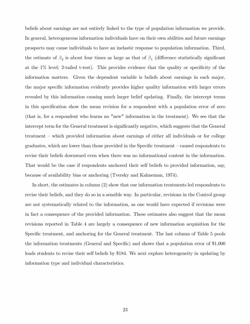
population earnings results in a revision of $184 in self earnings beliefs. This suggests that self

beliefs about earnings are not entirely linked to the type of public population information we

provide. There is, however, substantial heterogeneity in self earnings revisions in response to

information. First, the response to population earnings is more pronounced the more relevant

the information is�we �nd much stronger e¤ects in treatments where respondents are provided

with information on population earnings of graduates in speci�c majors than when they are

provided with information about earnings of all workers. More importantly, as in Eil and Rao

(2011) and Mobius et al. (2011), we �nd that the e¤ect of information is asymmetric: There

is signi�cant updating when the information is good news for the respondent, i.e., when the

respondent is informed that population earnings are higher than her prior beliefs: a revision of

$347 in self earnings beliefs for an underestimation of $1,000 in population beliefs, versus $159

for an overestimation of population earnings of the same magnitude.

In the second part of the paper, we estimate a simple model of Bayesian belief-updating

and ask how respondents�observed revisions compare to the case if they were Bayesian. In our

updating model, a Bayesian person would be one who treats the provided public information as

if it were private information. Given that the information we provide to respondents is for the

general population, ex-ante we expect that students would respond insu¢ ciently (relative to the

Bayesian benchmark) to the information. While our analysis shows substantial heterogeneity

in the information-processing heuristics used by students, it is somewhat surprising that nearly

40% of the students use the Bayesian or Alarmist (i.e., excessive updating compared to the

individual-speci�c Bayesian benchmark) heuristic. Nearly a third of the students either do not

respond to the information or respond less (�Conservative") than the individual-speci�c Bayesian

benchmark.

In analyzing the patterns of updating relative to the Bayesian benchmark, we document

some important heterogeneity in belief-updating. First, we do not �nd gender di¤erences in

information processing heuristics. Second, relative to freshmen, experienced students are more

likely to be non-updaters and less likely to react excessively to information (Alarmist updating).

Third, we �nd evidence of valence-based updating in the major-speci�c treatments: Respondents

4

are signi�cantly more likely to be Conservative and less likely to be Alarmist in their updating

when the news is negative, i.e., when they are informed that population earnings are lower than

their prior beliefs, than when the news is positive.

Finally, we assess whether our intervention leads to welfare gains in terms of major choice.

We �nd that the information on earnings we provide causes nearly half of the students to revise

their beliefs about graduating with the di¤erent majors. To get a sense of the impact of our in-

formation treatments on students�choices, we compute the welfare change �de�ned as change in

future expected earnings �for our sample. The mean welfare change in our sample is an increase

of $1,014 in age 30 earnings, and the welfare change is non-negative for three-quarters of our

sample. We also show that naively (counterfactually) imposing Bayesian updating would severely

overestimate the average welfare gains from our experiment. This highlights the importance of us-

ing actual data on belief-updating rather than relying on a homogeneous information-processing

rule.

While we show that our information intervention has a meaningful e¤ect on earnings beliefs

revisions, as measured within a survey, a relevant question is whether these e¤ects persist in

the long-run. For this purpose, we administered a follow-up survey to a subset of the treat-

ment respondents two years after the �rst survey, where we re-elicited their earnings beliefs

and probabilistic choices. We �nd that follow-up self earnings beliefs are more strongly corre-

lated with revised beliefs in the initial survey than with the baseline beliefs, indicative of our

�soft" information intervention having e¤ects that persist into the future. Our results suggest a

role for information campaigns, which tend to be cheaper than alternate intervention strategies.

However, the heterogeneity in belief-updating and the non-Bayesian updating exhibited by the

majority of our respondents also underscores the challenges in determining the e¤ectiveness of

such campaigns.

As mentioned above, our study design is motivated by the kinds of public information (about

returns to di¤erent types of educational investments) that students could encounter. At the same

time, our paper is related to the large experimental literature on information processing. One

strand of this literature explores the updating of ego-independent quantities such as which urn

5

a ball is drawn from (Grether, 1980; El-Gamal and Grether, 1995). The second category studies

information processing rules in settings that are more realistic and where beliefs have direct

importance such as ability, performance, climate change, risk assessment, and e¤ectiveness of

contraceptives (see, for example, Viscusi and O�Connor, 1984; Cameron, 2005; Delavande, 2008;

Eil and Rao, 2010; Mobius et al., 2011; Grossman and Owens, 2012). Our paper belongs to

the second category: We consider the updating of earnings expectations in the context of college

major choice�an important decision with signi�cant economic consequences. In addition, most

of the existing studies consider updating of binary outcomes, or have an information structure

where the signal is binary. Our setting is a hybrid design that combines experimentally manipu-

lated information as in laboratory experiments with a situation that is closer to real-world �eld

experiments. As a result, our setup di¤ers from the textbook case of Bayesian updating in two

ways. First, information revealed to students may already be known to them. Second, while

students are revising private beliefs about themselves, they receive public information. Both

these di¤erences have implications for the interpretation of our results. For example, our setup

should be biased against the �nding that respondents respond excessively to information. Yet,

we �nd that nearly a �fth of our respondents fall in this category. We show that our classi�cation

of updating heuristics is robust to these features of the study design.

The next section describes the data and experimental setup. Section 3 outlines a simple

model of expectations formation to explain the channels through which our information may

lead to systematic revisions of beliefs. The following two sections explore the heterogeneity in

population errors and analyze the patterns of revisions of self-earnings. Section 6 discusses the

signi�cance of the information experiment on measures of student welfare, and investigates the

long-term e¤ects of our intervention. Finally, Section 7 concludes.

6

2 Data

2.1 Administration

Our data is from an original survey instrument administered to New York University (NYU)

undergraduate students over a 3-week period, during May-June 2010. NYU is a large, selective,

private university located in New York City. The students were recruited from the email list

used by the Center for Experimental Social Sciences (CESS) at NYU. The study was limited to

full-time NYU students who were in their freshman, sophomore, or junior years, were at least 18

years of age, and US citizens. Upon agreeing to participate in the survey, students were sent an

online link to the survey (constructed using the SurveyMonkey software). The students could

use any internet-connected computer to complete the survey, and were given 2-3 days to start

the survey before the link became inactive. They were told to complete the survey in one sitting.

The survey took approximately 90 minutes to complete, and consisted of several parts. Students

were not allowed to revise answers to any prior questions after new information treatments was

provided. Many of the questions had built-in logical checks (e.g., percent chances had to be

between 0 and 100). Students were compensated $30 for successfully completing the survey.

2.2 Study Design

2.2.1 Treatment Group

The survey instrument consisted of three stages (see Figure 1):

1. Initial Stage: Respondents were asked their population beliefs�beliefs about the earnings

of current workers in the labor force, and self beliefs�beliefs about own earnings and other

outcomes, conditional on completing various majors.

2. Intermediate Stage: Respondents were randomly selected to receive 1 of 4 possible infor-

mation treatments. Each information treatment revealed statistics about the earnings and

labor supply of a certain group of the US population. The information was reported on

the screen and the respondents were asked to read this information before they continued.

7

Respondents were then re-asked their population beliefs (on areas they were not provided

information about) and self beliefs.

3. Final Stage: Respondents were given all of the information contained in each of the 4

possible information treatments. Respondents were then re-asked about their self beliefs.

The 4 information treatments consisted of statistics about the earnings and labor supply of

the US population. Table 1 lists the 4 information treatments:

1. All Individuals Treatment: revealed earnings for the population of all US workers currently

aged 30.

2. College Treatment: revealed earnings for the population of college graduates currently aged

30.

3. Female Major-Speci�c Treatment: revealed earnings for female bachelor degree holders

currently aged 30 by speci�c college major.

4. Male Major-Speci�c Treatment: revealed earnings for male bachelor degree holders cur-

rently aged 30 by speci�c college major.

We often combine results from the treatments where we classify the All Individuals and College

Treatments asGeneral treatments, and the Female and Male Major-Speci�c Treatments asMajor

Speci�c treatments. Students assigned to any one of these groups are treated with information,

and we refer to them as the "treatment group" below.

The information treatments were calculated by the authors using the Current Population

Survey (for earnings and employment for the general and college educated population) and the

National Survey of College Graduates (for earnings and employment by college major). Details

on the calculation of the statistics used in the information treatment are in Section A.1 of the

Appendix; this information was also provided to the survey respondents at the conclusion of the

survey. Survey respondents were randomly provided with one of these information treatments

in the intermediate stage. Before the population information was revealed, respondents were

8

asked about their prior beliefs about these population statistics. After revelation of information,

respondents were re-asked some of their self beliefs, including their subjective major-speci�c

earnings distribution at age 30.

The goal of this paper is to shed light on how students form earnings expectations. For that

purpose, we focus on updating of self beliefs for earnings. Respondents were asked about earnings

in their �rst job after college and for later periods at ages 30 and 45. Since the information about

population earnings pertained to current 30 year olds, we focus on updating of earnings reported

for age 30. In this paper, we use Initial Stage and Intermediate Stage beliefs in the analysis only.

2.2.2 Control Group

The mere act of taking a survey may prompt respondents to think more carefully about their

responses, and may lead them to revise their beliefs between the initial and intermediate stages

(see Zwane et al., 2011, for a discussion of how surveying people may change their subsequent

behavior). In order to identify the revision in self earnings beliefs directly attributable to infor-

mation, we recruited an additional group of students, whom we refer to as the "control group".

As in the treatment group, these students were asked about their population beliefs and self

beliefs in the Initial Stage. In the Intermediate Stage, however, these students were re-asked

their self beliefs but were not provided with any new information. Since we are interested in the

revisions in expectations caused by the new information, the di¤erences between the treatment

groups�and control group�s expectations allow us to identify that.

These students were recruited at a later date (April-May 2012), and were recruited the same

way as the students in the treatment groups. NYU students who had participated in the survey

for the treatment group were not eligible to participate in this survey. Students were compensated

$30 for successfully completing the survey (also constructed using the SurveyMonkey software),

and were required to come to the NYU CESS Laboratory to complete it.

9

2.2.3 Survey Instrument

We asked about earnings conditional on completing di¤erent college majors. Because of time

constraints, we were forced to make di¢ cult choices in the aggregation of college majors. We

aggregate college majors to 5 groups: 1) Business and Economics, 2) Engineering and Computer

Science, 3) Humanities, Arts, and Other Social Sciences (e.g. Sociology), 4) Natural Sciences and

Math, and 5) Never Graduate/Drop Out. We provided the respondents a link where they could

see a detailed listing of college majors (taken from various NYU sources), which described how

each of the NYU college majors maps into our aggregate major categories. Before the o¢ cial

survey began, survey respondents were �rst required to answer a few simple practice questions

in order to familiarize themselves with the format of the questions.

Expected earnings at age 30 were elicited as follows: "If you received a Bachelor�s degree

in each of the following major categories and you were working FULL TIME when you are 30

years old what do you believe is the average amount that you would earn per year?". We also

provided de�nitions of working full time ("working at least 35 hours per week and 45 weeks

per year"). Individuals were instructed to consider in their response the possibility they might

receive an advanced/graduate degree by age 30. Therefore, the beliefs about earnings we collected

incorporated beliefs about the possibility of other degrees earned in the future and how these

degrees would a¤ect earnings. We also instructed respondents to ignore the e¤ects of price

in�ation. The instructions emphasized to the respondents that their answers should re�ect their

own beliefs, and to not use any outside information.5

Our questions on earnings were intended to elicit beliefs about the distribution of future

earnings. We asked three questions on earnings: beliefs about expected (average) earnings,

beliefs about the percent chance earnings would exceed $35,000, and percent change earnings

would exceed $85,000. The last two were elicited as follows: "What do you believe is the percent

chance that you would earn: (1) At least $85,000 per year, (2) At least $35,000 per year, when

5We included these instructions: "This survey asks YOUR BELIEFS about the earnings among di¤erentgroups. Although you may not know the answer to a question with certainty, please answer each question as bestyou can. Please do not consult any outside references (internet or otherwise) or discuss these questions with anyother people. This study is about YOUR BELIEFS, not the accuracy of information on the internet."

10

you are 30 years old if you worked full time and you received a Bachelor�s degree in each of the

following major categories?".

We paid respondents a �xed compensation for completing the survey, and did not elicit

respondents�beliefs using a �nancially incentivized instrument such as a scoring rule. This is

because it is well known that proper scoring rules generate biases when respondents are not risk

neutral (Winkler and Murphy, 1970).6

2.3 Sample Statistics

A total of 616 students participated in the study: 501 students in the treatment group, and 115

students in the control group.

Since the analysis in the paper focuses on the heterogeneity in updating of students in the

treatment group, we describe their characteristics only (summary statistics for students in the

control group are similar, and the di¤erences in each of the demographic characteristics for the

two groups are not statistically di¤erent). For the treatment group, we drop 6 students who

report that they are in the 4th year of school or higher, violating the recruitment criteria, leaving

us with a total of 495 respondents. Table 2 shows the characteristics of our �nal sample. 36

percent of the sample (178 respondents) is male, 38 percent is white and 44.5 percent is Asian.

The mean age of the respondents is about 20, with 40.4 percent of the respondents freshmen,

36.4 percent sophomores, and the remaining juniors. Three-fourths of the respondents completed

the survey in under two hours, with 90% of all respondents completing the survey in 3.5 hours

or less. The average grade point average of our sample is 3.5 (on a 4.0 scale), and the students

have an average Scholastic Aptitude Test (SAT) math score of 699.5, and a verbal score of 682.5

(with a maximum score of 800). These correspond to the 93rd percentile of the corresponding

SAT population score distributions. Therefore, our sample represents a high ability group of

6It should be pointed out that even if respondents are risk neutral, incentivized belief elicitation techniquesare not incentive-compatible when the respondent has a stake in the event that they are predicting (the "nostake" condition in Karni and Safra, 1995), as is the case when reporting future earnings. In addition, Armantierand Treich (2011) show that beliefs are less biased (but noisier) in the absence of incentives. Finally, for selfbeliefs, we anyway do not have an objective measure against which their accuracy may be evaluated since we askrespondents for their individual self beliefs about future, unrealized, events.

11

college students.

3 Model of Earnings Expectations

We next outline a simple model of earnings expectations, focusing on how individuals may re-

spond to new information as in our information experiment. Let Xit be individual i�s expectation

at time t about earnings X.7 Moreover, let it denote i�s information set at time t. At the initial

stage, respondent i reports her beliefs about self earnings as:

Xit = E(Xjit):

= fi(it) (1)

The scalar valued function fi(�) maps the individual�s information set to self beliefs. In our

study design, we elicit self beliefs before and after a known perturbation of the individual�s infor-

mation set. This allows us to study the linkages between information and earnings expectations

represented by f(�).

We take a broad view of the individual�s information set. The individual�s information set

it contains both self information, such as the individual�s own perceived ability in a particular

�eld (derived from say previous test scores and coursework grades), and population information,

such as the individual�s perception of average earnings for workers with particular college ma-

jors. Note that we allow for the possibility that respondents�perceptions about the population

distribution could be di¤erent from the objective measures. Hence, the information set about

the population distribution of earnings could vary over time and across individuals. In this way,

some of the information the individual has can be considered �public" (common knowledge),

while other information can be considered �private" (known only to the individual). Since we

measure each individual�s beliefs about her own future earnings and her knowledge about the

population distribution of earnings, we can make some progress in distinguishing these two types

7Respondents report self earnings beliefs conditional on each major, if working full time, and for particularages, e.g. age 30. In this section, we ignore these details of our particular data collection.

12

of information.

Our information treatments provide information about the distribution of earnings of various

subgroups in the US population. Let Ii;t 2 it denote the scalar element of the information

set encompassing the information we provide in our experiment. Let i;t+1 and Ii;t+1 2 i;t+1

denote the new information set and new information after receipt of our information treatments,

respectively. After revelation of information, we re-elicit the respondent�s self beliefs about her

own earnings, denoted as Xit+1. There are two conditions which need to be met for an individual

to update her beliefs about future earning (i.e. Xit 6= Xit+1).

Condition 1) The information received in the new information treatment is new : At least

some of the information we provide has to be unknown to the individual, i.e. Ii;t 6= Ii;t+1 and

therefore it 6= it+1. Some individuals may already know the information we provide and

therefore not update their earnings. In this case, post-treatment expected self earnings Xit+1

would not systematically di¤er from initial self beliefs Xit.8

Condition 2) The information treatment is relevant : The individual�s expectations of fu-

ture earnings must depend in some way on information about population earnings we provide:

@fi(i;t)

@Ii;t6= 0. If the information about population earnings is not relevant to the individual�s

own earnings expectations, then our particular information treatments will not cause earnings

expectations to be updated.

Before we turn to the empirical results, we note that there are several ways in which indi-

viduals can update their self earnings expectations with respect to potentially new information

about population earnings. The magnitude of revisions depends on the exact function that

maps population earnings to self beliefs; in general, we expect proportional responses in updat-

ing (larger revisions for larger misperceptions about population earnings), but that need not be

the case. Similarly, we would expect downward revisions in self earnings beliefs if the respon-

dent over-estimates population earnings, and upward revisions of self earnings if the respondent

under-estimates population earnings. However, this need not necessarily be the case: for exam-

8There is a possibility that being exposed to already-known information causes a respondent to revise her selfearnings beliefs because of saliency and/or availability bias (Tversky and Kahneman, 1973; Dellavigna, 2009).For that to be the case, the function fi(:) that maps events to self beliefs, Xit = fi(it), has to be time-varying.We do not consider that case here.

13

ple, an individual who learns that she under-estimated population earnings in a �eld may be led

to believe that the population of workers in a �eld are in fact of much higher ability than she

previous thought. To the extent that the individual believes that earnings are largely assigned

based on relative ability, then under-estimating population earnings may lead the individual to

revise her self earnings beliefs downward.

In contrast, consider the restrictions standard Bayesian updating places on the expectations

updating. In a Bayesian updating model, for beliefs that are characterized by the beta distribu-

tion, the posterior (updated belief) Xi;t+1 = E[Xji;t+1]:

XBayesi;t+1 = wXit + (1� w)Ii;t+1 (2)

whereXit is the prior belief, Ii;t+1 is the new information we provide in our information treatment,

and w = V (Xit)�1

V (Xit)�1+V (Ii;t+1)�1is the weight associated with the prior belief, speci�ed as a function

of the uncertainty or variance of the prior relative to the new information. Then, the relative

weight placed on the information is V (Xit)V (Ii;t+1)

, i.e., responsiveness to information should be directly

proportional to the uncertainty in the prior beliefs. The standard Bayesian case in equation (2)

places restrictions on the fi(�) general updating function in (1). In particular, it assumes that

fi(�) is linear and separable in Ii;t+1. Our research design allows us to test these restrictions

since we collect data on prior beliefs and updated beliefs. We use this data to characterize the

heterogeneity in updating behaviors, and estimate the fraction of the population that updates

in the particular Bayesian way.9

There are two important di¤erences between our experimental design and the textbook case

of analyzing Bayesian updating. First, the information we reveal may already be known by

some respondents (a violation of Condition 1). As we show below, this is not the case for our

respondents since all individuals had some errors in their beliefs about the population earnings

distribution. However, the distribution of errors in population beliefs, discussed below, shows that

there is substantial heterogeneity in how informative the information provided to respondents

9The Bayesian case also implicitly assumes that the respondent �nds the information fully credible, and thatIi;t+1 is equal to the true population information that is provided to the respondents.

14

was. A second key di¤erence in our experimental design from the textbook case is that we reveal

population information but ask individuals about their self beliefs about themselves. Individuals

can di¤er in how relevant they believe the population distribution of earnings is to their own

self future earnings, that is, the function fi(�) mapping population earnings to self beliefs may

vary across individuals. For example, if we observe that a respondent does not revise her beliefs

in response to the information, even after controlling for her priors about the information, this

could either imply biased, non-Bayesian, updating, or that the respondent simply did not �nd

information on population beliefs relevant for self beliefs (a violation of Condition 2). We discuss

implications of this later.

The di¤erence between the interpretation of the Bayesian updating we analyze and the text-

book case is a consequence of our experimental setup. In typical studies of belief updating

(Tversky and Kahneman, 1974; Grether, 1980; Viscusi and O�Connor, 1984; and Viscusi, 1997;

Cameron, 2005; El-Gamal and Grether, 1995; Eil and Rao, 2011; Mobius et al., 2011), respon-

dents are provided with (noisy) private signals about the same quantity over which revision of

beliefs are being analyzed. For example, in the frameworks used by Eil and Rao (2011), Mobius

et al. (2011), and Grossman and Owens (2012), respondents are revising their beliefs about

either their own intelligence or beauty, and receiving feedback about the same underlying entity

for which beliefs are being reported. That is not the case in the design used in our study: We

observe belief updating about future self earnings, formed from past population and self signals,

whereas the signals that students receive in our experiment are about population beliefs. Our

study design is motivated by the kinds of information that are typically available to students

when making real world schooling choices.10 Information along similar lines has been provided

in other contexts, and it has been shown to have an impact on actual schooling choices (Jensen,

2010; Nguyen, 2010).

In the next section, we analyze the subjective earnings data, and investigate average revisions

10The kind of information that we provided to respondents is precisely the kind that are available in main-stream sources. For example, the Chronicle of Higher Education lists earnings by major and subject area:http://chronicle.com/article/Median-Earnings-by-Major-and/127604/ (accessed December 24, 2012). Similarly,the BLS publishes a yearly handbook with information on earnings, job prospects, and working conditions etc.at hundreds of di¤erent types of jobs in the Occupational Outlook Handbook (http://www.bls.gov/oco/).

15

in earnings. Heterogeneity in belief-updating is investigated in a later section.

4 Earnings Beliefs and Revisions

In this section, we examine self beliefs about what each individual expects to earn in di¤erent

majors, beliefs about population average earnings, and revisions in self beliefs following the

information treatment. The analysis is restricted to students in the treatment group, except in

the case where we analyze revisions in self beliefs; then, we also include students in the control

group, since their responses allow us to infer the causal e¤ect of information.

4.1 Self Beliefs about Earnings

We �rst describe self beliefs about own earnings at age 30 if the respondent were to graduate

in each major. The �rst column of Table 3 reports the average, median and standard deviation

of the distribution of reported average self earnings in our sample at the Initial Stage. At

the Initial Stage of the experiment all subjects were asked the same baseline set of questions.

Looking across majors in column (1), we see that students expect the highest earnings ($128,460)

if they major in economics/business, and lowest if they do not graduate ($38,750). Among the

graduating majors, students expect the earnings to be lowest in humanities and arts ($66,450).

The median point forecast is substantially lower than the mean self earnings for all majors,

indicating that the distribution of point forecasts of future earnings is right-skewed. There is

also considerable heterogeneity in self beliefs as indicated by the large standard deviations. The

extent of heterogeneity can also be viewed in the top panel of Appendix Figure A1, which shows

the belief distribution of our respondents if they were to graduate in economics or business. For

example, in the economics and business category, the 5th percentile of the self belief distribution

is $50,000, the 50th percentile is $90,000, and the 95th percentile is $300,000. The second column

of Table 3 reports self earnings for the subset of students who report to be either majoring or

intending to major in that �eld. Compared to the beliefs for the full sample (column 1), this

group of students has higher mean beliefs in all majors. This is consistent with observed sorting

16

by ability and positive selection into majors based on expected earnings (Arcidiacono, 2004;

Gemici and Wiswall, 2011).

As described above, we also collected data on the subjective distribution of future earnings.

For this purpose, students were asked about the probability they would earn at least $35,000 and

at least $85,000 at age 30 if they were to graduate in each major. Columns (3) and (4) of Table 3

present the average probabilities reported by students. While students believe that the likelihood

of earning at least $35,000 is fairly similar across the graduating majors (at least 74 percent),

the subjective likelihood of earning at least $85,000 varies substantially across the majors, with

students expecting the highest probability of that happening in the economics/business and

engineering/computer science categories (mean probability exceeding 60 percent in both), and

the lowest probability in humanities/arts (44 percent) among the graduating majors. It is not

surprising that students report low probabilities for the occurrence of these outcomes in the

no-degree major.

4.2 Population Beliefs about Earnings

At the beginning of the Intermediate Stage, we divided the treatment subject pool into 4 ran-

domly selected information treatment groups and asked corresponding baseline population beliefs

questions before we provided the information treatment. We asked the following question for the

randomly selected subset of respondents who were later assigned the Male Major-Speci�c Treat-

ment: "Among all male college graduates currently aged 30 who work full time and received a

Bachelor�s degree in each of the following major categories, what is the average amount that you

believe these workers currently earn per year?". For another randomly selected group of respon-

dents who were later assigned the Female Major Speci�c Treatment, we asked the corresponding

question about female graduates.

Columns (5) and (6) of Table 3 report the mean, median and standard deviation of beliefs

about US population earnings of men and women by the 5 major �elds, reported by the two

subsets of our sample who received the Major-Speci�c (Male or Female) treatments. Self beliefs

may di¤er from population beliefs for several reasons: Students might think that future earnings

17

distributions will di¤er from the current ones, or students may have information about themselves

that justi�es having di¤erent expectations. The di¤erence between self and population beliefs

therefore provides some suggestion of the student�s belief of their own earnings advantage or

disadvantage relative to the population average.

Looking across each of these columns, we see that population beliefs follow the same pattern

as self beliefs (columns 1 and 2), with students believing population earnings to be highest in the

economics/business and engineering/computer science categories, and lowest in humanities/arts

and the not graduate categories. Compared to self earnings beliefs, students report lower pop-

ulation beliefs for most major categories. It is also interesting to note that students accurately

perceive a wage gap in favor of men in most �elds, with median earnings for males exceeding those

for females in all �elds except natural science; however, the average beliefs show that students

perceive higher earnings for males in economics/business and engineering/computer science only.

For the other, more general, information treatments, respondents randomly assigned to the All

Individuals Treatment were asked the following question about their population beliefs: "Among

all individuals (college and non-college graduates) currently aged 30 who work full time, what is

the average amount that you believe these workers currently earn per year?". Those in the College

Treatment were asked about earnings of all college graduates currently aged 30 and working

full time. Mean population beliefs in the All Individuals Treatment are $46,900, substantially

lower than those for all majors, except the no graduate category. This demonstrates that,

at least in the aggregate, respondents accurately believe that college graduates have higher

average earnings than the full population. In the College Treatment, the mean belief reported for

college graduates is $80,190, higher than that reported for humanities/arts in the Major Speci�c

treatments, accurately re�ecting that the college graduate population includes individuals with

higher earning majors. As with all of the population beliefs about college major speci�c beliefs,

there is substantial heterogeneity in the population beliefs about college graduates.

18

4.3 Errors in Population Beliefs

In the case of the groups receiving the Male and Female Major Speci�c treatments, the compar-

ison of population beliefs (columns 5 and 6 of Table 3) in a given major with true population

earnings (reported in Table 1) in the corresponding major shows that average student beliefs

over-estimate the true average population earnings for all �elds, except male earnings with the

no-degree major. Columns (7) and (8) of Table 3 report the mean absolute error, de�ned as

the absolute value of the di¤erence between the true and perceived population earnings. We

use the absolute value of the error here to assess the magnitude of the errors, without positive

and negative errors canceling out. The mean absolute errors are substantial, varying from a

mean of $15,770 for female no-degree workers to $45,730 for male workers who graduated in eco-

nomics/business. Students also have considerable errors about the population average earnings

for all workers and for college educated workers: the absolute error in population beliefs for all

workers is $12,760, and for college-educated workers is $32,620.

The large standard deviations on the absolute errors in columns (7) and (8) suggest that

population errors are quite heterogeneous.11 Appendix Table A1 shows that this heterogeneity

in population errors is not systematically related to observable characteristics of individuals.

4.4 The Impact of Information on Self Beliefs

We next explore how self beliefs are revised as the student respondents receive the information

treatments. Table 4 reports the mean and standard deviation of the distribution of revisions

(intermediate-initial stage) in self beliefs about earnings. The �rst column shows that the mean

revision in self beliefs for the treatment group is -8.14, that is, an average downward revision

of $8,140. This is larger than the mean revision of -$3,850 in self beliefs for the control group,

reported in the second column (di¤erence not statistically signi�cant). Since positive and negative

11The middle panel of Figure A1 shows the distribution of raw population errors regarding full-time females�earnings with an economics or business degree. Here raw errors are de�ned as truth-belief, such that a negativeerror indicates over-estimation of the truth, and a positive error indicates under-estimation of the truth. Re�ectingthe dispersion in baseline beliefs, there is considerable heterogeneity in the level and sign of the errors, with non-trivial numbers of students making both positive and negative errors in all categories. However, the distributionis skewed to the left: the median of this error distribution is -$19,270 (i.e., over-estimation of population earningsby $19,270), the 5th percentile is -$139,270 and the 95th percentile is $10,730 (under-estimation).

19

revisions may cancel out, we also report the absolute percent revisions. The average absolute

revisions reported in square brackets are substantially larger, indicative of a non-trivial proportion

of revisions in both directions. Notably, the average absolute revision in the treatment group is

signi�cantly larger than that in the control group ($26,550 versus $13,140).

The remaining rows of the table show that there is considerable heterogeneity in the updating

of self beliefs across majors. For the treatment group, the average of the percent revisions

distribution varies from -$28,540 (downward revision) in economics/business to +$8,560 (upward

revision) in the no-degree category. As indicated by the standard deviations, within categories

there is considerable heterogeneity.12 The �rst two columns also show that average revisions in

the treatment group are larger than those in the control group. In fact, for all �elds except the

no-degree category, average absolute revisions in the treatment group are signi�cantly di¤erent

(and larger) than those of the control group at the 15% signi�cance level or higher. This suggests

that our information treatments caused students to revise their beliefs.

Columns (3) and (4) of Table 4 show the revisions of self beliefs in the combined Major-

Speci�c (Female and Male) and General (All Individuals and College) treatments, respectively.13

It is interesting to note that the mean revisions in the Major-Speci�c and General treatments are

qualitatively similar in magnitude; the revisions are statistically di¤erent only for the no-degree

category. Recall that in the General treatment, students receive information about earnings

for either all individuals or for college graduates. This �nding would seem to contradict the

hypothesis that the General treatment is less relevant to individual self beliefs than the Major-

Speci�c treatment. However, if individuals respond to the overall level of the information relative

to self beliefs and do not �nd the information provided in the General treatment irrelevant, the

fact that the General treatment provides lower values for average earnings may cause a greater

12The bottom panel of Figure A1 shows the dispersion in students� percent revisions for earnings in eco-nomics/business in the Female Major-Speci�c Treatment: the 5th percentile of the earnings revision is -75 percent,the 50th percentile is -18.75 percent, and the 95th percentile is +33.33 percent.

13For much of the remaining analysis, we pool the responses in the All Individuals and College treatmentsinto the �General" treatment, and the Female and Male Major-Speci�c treatments into the �Major Speci�c"treatment. This is because the results are qualitatively similar when we analyze the All Individuals and Collegetreatments separately, and when we analyze the Female and Male Major-Speci�c treatments separately. Poolingin this way keeps the tables simple.

20

downward revision than the Major-Speci�c treatment.14

The same information is presented slightly di¤erently in Column (1) of Table 5, which re-

gresses the dollar amount revisions in self earnings onto dummies for the Control group, the

Speci�c treatment, and General treatment. Standard errors in these regressions are clustered at

the individual level, since we have �ve observations per individual (one for each of the �ve major

categories). The notable �nding is that the average revision for the Control group is noisy and

not statistically di¤erent from zero. On the other hand, both the General and Speci�c treatments

lead to substantially larger (and statistically di¤erent from zero) downward average revisions.

Thus, our information treatments do seem to lead students to revise their self beliefs. The similar

average revisions in both the General and Speci�c treatments suggest that the speci�city of the

information does not seem to matter. We next explore if students respond to the information in

a "meaningful" way.

4.5 Are Revisions in Self Beliefs Sensible?

As outlined in our model of expectations formation in Section 3, if students perceive a link

between population earnings and self beliefs (i.e., perceived population earnings is a relevant

element of the respondent�s information set used to report self earnings beliefs), then revealed

errors in population beliefs should be systematically related to revisions of self beliefs. We test

(1) whether revisions in self beliefs are, on average, positively related to population errors (for

example, if a respondent underestimates the population earnings, the respondent revises her self

beliefs upwards), and (2) whether revisions are proportional to the error in population earnings.

The updating patterns in Table 4 and population beliefs reported in Table 3 hint towards a

14Recall that our experimental design for the treatment group has two rounds of information provision, onein the intermediate stage and one in the �nal stage. In the �nal stage, all respondents were provided with theinformation from all 4 treatments. Thus, at the start of the �nal stage, all students have the same information,although they have received this information in a di¤erent order. We �nd that the most notable changes in meanrevisions in the �nal stage occur for respondents who were assigned to the General treatment. This is as one wouldexpect since the General treatment respondents should be the ones who �nd the new information provided in the�nal stage most valuable. We also �nd that being exposed to di¤erent information in the intermediate stage doesnot have an anchoring e¤ect on respondents�revisions (Tversky and Kahneman, 1974): Regardless of whetherthe respondents were assigned to the General or Speci�c treatment in the intermediate stage, mean revisions inthe �nal stage for the two sets of respondents are statistically similar in all the �ve major �elds (results availablefrom the authors upon request).

21

logical positive relationship between the two. We see that students, on average, revise downward

their self earnings beliefs the most in economics/business, which is the �eld with the highest

average over-estimation in population earnings (compare population beliefs in columns (5) and

(6) of Table 3 with true population earnings in Table 1). Similarly, self beliefs are revised upward

the most for the not graduate category, which is the �eld with the largest under-estimation in

population earnings.

To explore the link between revisions in self beliefs and errors, we estimate a series of reduced-

form regressions of the form:

Xi;m;t+1 �Xi;m;t = DControli +DSpecT

i +DGenTi + �1(Errori;m �DControl

i ) + �2(Errori;m �DSpecTi )

+�3(Errori;m �DGenTi ) + "i;m;

where the dependent variable is the change (intermediate - initial) in age 30 self earnings reported

by respondent i for major m, and the dummy DTi equals 1 if i is assigned to group T , where

T = fControl; Specific, Generalg. The parameters of interest are the betas: for example, �1is the revision response to a unit change in error in population beliefs (recall that, the error is

de�ned as true population earnings - perceived population earnings). Respondents in the Control

group do not receive the true population earnings, but we can still construct their population

error. Since this error is never revealed to them, we would expect no systematic relationship

between revisions and population error for the Control group. On the other hand, for sensible

updating caused by our information treatment, we expect estimates of �2 and �3 to be positive,

and to be statistically di¤erent from zero. Column (2) of Table 5 reports the OLS estimates of

this speci�cation. Four things are of note: First, �1 is small in magnitude and not statistically

di¤erent from zero, while both �2 and �3 are positive and estimated very precisely. This is

evidence of logical updating in response to our information treatments. Second, the estimates

of �2 and �3 show that the response of revisions in self beliefs to population errors is relatively

�inelastic"; for example, an error of $1,000 in population beliefs results in a revision of $337 in

self earnings in the Speci�c treatments (and $86 in the General treatments), suggesting that self

22

beliefs about earnings are not entirely linked to the type of population information we provide.

In general, heterogeneous information individuals have on their own abilities and future earnings

prospects may cause individuals to have an inelastic response to population information. Third,

the estimate of �2 is about four times as large as that of �1 (di¤erence statistically signi�cant

at the 1% level; 2-tailed t-test). This provides evidence that the quality or speci�city of the

information matters. Given the dependent variable is beliefs about earnings in each major,

the major speci�c information evidently provides higher quality information with larger errors

revealed by this information causing much larger belief updating. Finally, the intercept terms

in this speci�cation show the mean revision for a respondent with a population error of zero

(that is, for a respondent who learns no "new" information in the treatment). We see that the

intercept term for the General treatment is signi�cantly negative, which suggests that the General

treatment �which provided information about earnings of either all individuals or for college

graduates, which are lower than those provided in the Speci�c treatment �caused respondents to

revise their beliefs downward even when there was no informational content in the information.

That would be the case if respondents anchored their self beliefs to provided information, say,

because of availability bias or anchoring (Tversky and Kahneman, 1974).

In short, the estimates in column (2) show that our information treatments led respondents to

revise their beliefs, and they do so in a sensible way. In particular, revisions in the Control group

are not systematically related to the information, as one would have expected if revisions were

in fact a consequence of the provided information. These estimates also suggest that the mean

revisions reported in Table 4 are largely a consequence of new information acquisition for the

Speci�c treatment, and anchoring for the General treatment. The last column of Table 5 pools

the information treatments (General and Speci�c) and shows that a population error of $1,000

leads students to revise their self beliefs by $184. We next explore heterogeneity in updating by

information type and individual characteristics.

23

4.5.1 Heterogeneity in Updating by Information Type

Table 6 explores the heterogeneity in updating. Since we are interested in heterogeneity in

updating in response to the information, the analysis in this table is restricted to respondents in

the information groups, that is, the General and Speci�c treatments. The �rst column repeats

the speci�cation similar to that reported in the last column of Table 5, that combines the General

and Speci�c treatments (and excludes Control respondents).

Panel A investigates heterogeneity by information type. One dimension of information type

is the direction of the errors revealed by the information. While students are responsive to

both under- and over- estimation of population earnings, column (2) shows that response to

information is asymmetric. A positive error, i.e., under-estimation of population earnings, results

in larger updating: An under-estimation of population earnings by $1,000 results in an upward

revision in self earnings of $347, compared with a downward revision of $159 for a $1,000 over-

estimation of population earnings (the estimates are, however, not di¤erent at conventional levels

of signi�cance; p-value = 0.327). Therefore, self beliefs seem to be more responsive to information

when it is good news�that is, when the respondent is informed that population earnings are

higher than her prior beliefs. This pattern of asymmetric updating is consistent with Eil and

Rao (2011), and Mobius et al. (2011), who �nd beliefs to be relatively more responsive to good

news (where good news is de�ned as feedback that improves one�s self-image).15

Column (3) of Table 6 shows that response to information revealed in the Speci�c treatments is

larger when the respondent�s gender is the same as that for which population earnings information

is provided. The estimates indicate that a female respondent revises her self beliefs by $439 in

the Female Major-speci�c treatment for a population error of $1,000, compared with a revision

of $284 in the Male Major-speci�c treatment (coe¢ cients statistically di¤erent with a p-value of

0.02). This provides evidence that the speci�city of the information matters: respondents are

more responsive to information that it is more relevant for them.

15We conducted an additional set of regressions in which the error is interacted with various treatment char-acteristics, and the e¤ect of the error is allowed to vary depending on whether the information is positive ornegative. We see that, in almost all the speci�cations, greater (economic and statistical) signi�cant updatingarises in instances of positive errors. Results available from the authors upon request.

24

4.5.2 Heterogeneity in Belief Updating by Individual Characteristics

We next explore the extent of heterogeneity in the relationship between population errors and

earnings beliefs using a set of observable characteristics for respondents. In column (4) of Panel B

of Table 6, we include an indicator for female gender, and interactions of the error with female and

male indicators. Estimates for the interaction terms indicate that both men and women logically

update their beliefs (a positive coe¢ cient), but females are signi�cantly more responsive to their

population errors (the coe¢ cients are statistically di¤erent at the 1% level). This suggests a

strong gender di¤erence in responsiveness to population errors.

The second regression in Panel B investigates whether responses to the information treatment

di¤er by the grade level of the student. The interaction terms indicate that freshman, sopho-

mores, and juniors all update logically to errors. However, contrary to what one would expect,

students in later years �who should have greater private information about themselves �are

more responsive to their population errors; the response is still inelastic for each of the groups.

Finally, the third column of Panel B (column 6) investigates whether there is heterogeneity in

updating by the ability of the student, where we classify students as high ability if they have an

SAT score greater than 1450 (30% of our sample respondents fall in the high ability group). The

interaction terms reveal that low and high ability students are equally responsive to errors they

make (the estimates are not statistically di¤erent; p-value = 0.715).

4.5.3 Belief Updating and Uncertainty

In a Bayesian framework, ceteris paribus, respondents who are more uncertain about future

earnings should be more responsive to the treatment information. In order to determine the

uncertainty about future earnings, we use the variance obtained from �tting a log-normal distri-

bution to each respondent�s percentile responses (subjective beliefs of earning more than $35,000

and $85,000 per year). We de�ne a "High Variance" dummy variable, that equals 1 if the respon-

dent�s variance is above the cross-sectional median variance. The regression in Panel C of Table

6 interacts the error term with high and low variance dummy variables. As one would expect

in a rational (i.e., Bayesian) updating framework, the responsiveness to information is driven by

25

respondents who have greater uncertainty about future earnings: the estimate for high-variance

respondents is an order of magnitude larger than that for low-variance respondents, and the

estimates are statistically di¤erent (p-value = 0.000). In an additional set of regressions (not re-

ported here), we interact the variance dummy with other treatment characteristics. In all cases,

we �nd evidence of signi�cant updating for high-variance (i.e., greater uncertainty) respondents,

but not for low-variance respondents.

4.5.4 Non-Parametric Analysis

To further explore the relationship between errors and belief updating, we turn to a non-

parametric analysis using a local linear regression. Figure 2 shows the local linear regression

of self earnings revisions on population errors. We pool the General and Speci�c treatments in

the �gure, since the patterns are qualitatively similar otherwise. Two points are of note. First,

the response of revisions to errors is asymmetric, with a steeper slope for positive errors; this

is consistent with our �nding in column (2) of Table 6. Second, even conditioning on direc-

tion of error, the relationship does not seem to be linear. In the next section, we explore the

heterogeneity in updating in more detail.

Before we move on to characterizing the heterogeneity in updating, we brie�y discuss the

concern of measurement error in the subjective data. Subjective data, like most data, su¤er

from measurement error. One concern, therefore, in using these data is that measurement er-

ror would be exacerbated using di¤erences. However, the systematic relationship between self

earnings revisions and population errors that we observe for the treatment groups suggests that

measurement error alone cannot be driving the revisions. If the responses we receive are purely

measurement error, we would expect no systematic relationships between self earnings revisions

and population errors, as is the case for the Control group. In Section A.3 of the Appendix we

show that the data yield a reliability ratio of 0.984, indicating that measurement error is not a

serious concern in the data.

26

5 Characterizing the Heterogeneity in Belief Updating

Section 4 shows that our information experiment had an e¤ect on earnings beliefs, with substan-

tial heterogeneity in self beliefs revisions. We also �nd that the revision patterns are consistent

with a Bayesian updating model. In this section, we further investigate the heterogeneous up-

dating patterns of the treatment respondents. In particular, we are interested in exploring how a

respondent�s belief about expected self earnings reported in the intermediate stage�the Observed

posterior�compares to a posterior if the updating process were approximately Bayesian, i.e., the

Bayesian posterior.

5.1 Bayesian Benchmark

We use our information experiment to construct a Bayesian benchmark level of updating for each

respondent and then compare the actual observed updating for each individual to this benchmark.

If the updating process were Bayesian, the posterior self earnings belief for each major would be

given by (2). The actual revised earnings beliefs are given by Xi;t+1. The constructed Bayesian

posterior from (2) is given by XBayesi;t+1 . In our speci�c setup, Xi;t+1 is respondent i�s belief in

the Intermediate stage about expected self earnings in a particular major; the prior Xit is the

belief reported in the Initial stage about expected self earnings in each major; and information

treatment Ii;t+1 is the information treatment that i is provided about earnings between the

Intermediate and Initial stage.16 The variance of the prior V (Xit) is the individual-speci�c

precision of the prior; and V (Ii;t+1) is precision of the revealed population information. Since

the information is about population earnings, the precision associated with this information is

homogeneous, i.e. Ii;t+1 = It+1 for all i.17

16For simplicity, we do not index these by major, but each variable is major speci�c; e.g. we elicit beliefs aboutearnings if the individual would major in economics/business.

17In the General treatments, since the respondent is provided with population earnings of either all workers orcollege graduates, there is only one piece of new information that is observed for each major. In the Major-Speci�ctreatments, we assign the respondent the information about population earnings in the major corresponding tothe self beliefs about earnings in each major. Therefore, in this case, V (Ii;t+1) varies by major. We assume thatin the Major-Speci�c treatments, information about population earnings in only the particular major (and notthe other �elds) a¤ects earnings beliefs in that major. We �nd evidence consistent with this in reduced-formregressions where we regress revisions in self earnings onto population errors in the di¤erent majors.

27

To compute the variance of future earnings, recall that students were asked about the prob-

ability of earning at least $35,000 and $85,000 at age 30 if they were to graduate in each major

(both before and after receipt of information), and they were also provided with information

about the distribution of population earnings. We �t the responses of the respondent to the

questions about the chance of earning more than $35,000 and more than $85,000 per year to

a log-normal distribution, and obtain an estimate of V (Xit) and V (Xi;t+1) for each major and

individual. Similarly, we use the empirical likelihood of earning more than $35,000 and $85,000

in the population �information that students were provided with in the treatments �to obtain

an estimate of V (It+1).

5.2 Are Students Bayesian?

We next investigate how the actual earnings beliefs we observe in our information experiment

compare to the Bayesian benchmark. Figure 3 plots the observed updating in average self

earnings (Xi;t+1 �Xit) and the Bayesian revision (XBayesi;t+1 �Xit). We pool the majors together,

since the plots are otherwise similar. The �gure shows the �tted lines from an OLS regression of

observed revision on Bayesian revision, for both the General and Speci�c treatments. If students

are Bayesian, the lines of best �t should overlap with the 45-degree line. The �tted lines are,

however, �atter than the 45-degree line for both treatments. This indicates that, on average,

students respond less to the information than the Bayesian benchmark. The �gures also show less

sensitivity to the information in the General treatments (note, however, that the OLS estimates

for the General and Speci�c treatments are not statistically di¤erent from each other).

5.2.1 Characterizing Belief Updating Heuristics

We next characterize the updating heuristics used by our respondents. We classify each respon-

dent to an updating type, depending on how her observed posterior compares with our Bayesian

benchmark posterior. We use �ve possible heuristics to classify a respondent�s updating. A

respondent�s type is: (1) Bayesian if her posterior belief is within a band around the Bayesian

posterior; (2) Alarmist if, relative to the Bayesian benchmark, the response is more exaggerated;

28

(3) Conservative if she updates in the right direction but less than a Bayesian; (4) Contrary

if the updating is in the opposite direction, i.e., inconsistent with the direction prescribed by

Bayesian updating; and (5) Non-Updater if there is no response to the information. We borrow

this nomenclature from the previous psychological and experimental economics literature on be-

lief updating (Grether, 1980; Kahneman and Tversky, 1982; El-Gamal and Grether, 1995). This

literature classi�es individuals as using the Conservative heuristic if they fail to su¢ ciently adjust

their beliefs in light of new information, and classi�es individuals as using the "Representative"

heuristic if they rely too heavily on recent information; we instead use the term "Alarmist" to

refer to such updating.

Section A.2 of the Appendix outlines the empirical criteria used for assigning an updating

heuristic to a respondent for updating in a given major. The respondent is classi�ed as being

Bayesian if her revised belief lies within a band around the Bayesian posterior. Excessive (inex-

cessive) updating relative to the band would lead to the respondent being classi�ed as Alarmist

(Conservative).

Note that in the textbook Bayesian framework, any non-Bayesian updating is considered

irrational. That, however, is not the case in our more general framework. As we explain in

Section 3, if a respondent already knows the population information we provide or, more likely,

does not consider population earnings information relevant for her own self earnings, she would

not revise her self beliefs (i.e., she would be a Non-Updater type). Moreover, as outlined in

Section 3, it is possible that a respondent revises her beliefs in the opposite direction of her

errors if population earnings information leads her to primarily update her own relative ability

beliefs. This could explain the updating of some respondents classi�ed as Contrary.18

18Equation (2) treats the information provided in the Speci�c and General treatments similarly, i.e., it isassumed that the information is equally valuable in both treatments. However, the Speci�c treatments providehigher quality information and, from Table 6, we know that students are more responsive to the information inthe Speci�c treatments. Therefore, ex-ante, we should expect to see fewer respondents being Bayesian or Alarmistin the General treatments.

29

5.2.2 Distribution of Updating Types

Using the classi�cation in Appendix equation (A1), we determine the distribution of respondents�

types based on their earnings updating in their own (intended) major. Table 7 reports the

distribution of types separately for the Speci�c and General treatments. Looking across column

(1), we see that nearly a �fth of the sample respondents are non-updaters, i.e., they do not change

their self beliefs on receipt of information. Among the respondents who revise their beliefs, the

most common heuristic is either Bayesian updating, with 27-32 percent of the sample using this

heuristic. A substantial proportion of respondents are conservative in their updating. Finally,

12-19 percent of the respondents are Contrary, i.e., they update in a way that is not consistent

with the Bayesian updating model.19

Because our design included di¤erent kinds of population information, from general infor-

mation about earnings for all workers to more speci�c information about earnings by particular

gender and major, some individuals could �nd the general information not relevant but the

major-speci�c information relevant. We might expect then the relative share of Conservatives

to be larger in the General treatment, and that of Bayesian and Alarmist respondents to be

smaller. In fact, there are only half as many Alarmists in the General treatment than in the

Speci�c treatments; the two type distributions are statistically di¤erent (p-value = 0.021, for a

Chi-square test of the equality of the type distributions). However, it is quite surprising that

nearly a third of the respondents in the General treatment are Bayesian, i.e., they treat infor-

mation about earnings for all workers and college graduates in a way analogous to how private

signals would be treated.

The remaining columns of Table 7 report the distribution of heuristics for various sub-samples.

Columns (2) and (3) show the gender-speci�c distribution of types. In the Major-Speci�c treat-

ments, women, relative to men, are more likely to update; and conditional on updating, more

likely to be Bayesian or Alarmist. The reverse patterns are observed for the General treatments.

Overall, we cannot conclude that there are any systematic di¤erences by gender (as is also indi-

19In instances of missing data on either average earnings or beliefs about earnings being above certain thresh-olds, the respondent�s type cannot be classi�ed. That is the case for about 10% of the respondents, for whom theheuristic is thus unde�ned.

30

cated by the Chi-square test for the equality of the distributions).20 Columns (4) and (5) show

the type distribution for freshmen and upperclassmen (sophomores and juniors). Two di¤erences

between the two groups are of note. First, compared to freshmen, a larger proportion of upper-

classmen do not update. This suggests that through their more extensive college experience,

upperclassmen have gathered more private information about their own future earnings. Second,

freshmen are much more likely to use Alarmist updating, than upperclassmen. With regards to

ability (columns 6 and 7 of Table 7), we see that high ability respondents are less likely to update

in the General treatments, and are more likely to react excessively to information in the Speci�c

treatments.

The last two columns of Table 7 show the distribution of types for respondents with positive

errors (i.e., those who underpredict population earnings) and negative errors, respectively. The

type distribution is similar in the case for the General treatments, with nearly a third of respon-

dents being Bayesian and another third using either the Non-updater or Conservative heuristic.

However, the type distribution di¤ers systematically in the Speci�c treatments (p-value = 0.013

for a Chi-square test, rejecting the equality of the type distributions). The most common heuris-

tic for respondents who make positive errors is Alarmist updating, i.e., they respond excessively

to the information. We see that students are much more likely to be conservative in their updat-

ing when their population error is negative compared to when it is positive (16% of the sample

in the negative-error case, versus 1.4% of the sample in the positive-error case). Therefore, this

suggests that there is valence-based updating. Students tend to react (excessively) when the

information is good news, i.e., when they receive the news that population earnings are higher

than their priors.

In additional analysis not reported here, we also classify the respondent�s type for the four

other major categories that the student reports is not their primary "intended" major. While

students use a mixture of heuristics across the four majors, we �nd that there is consistency in

20This is at odds with Mobius et al. (2011) who �nd substantial gender di¤erences in both informationprocessing and information acquisition. Possible explanations for these di¤erent �ndings could be that studentsin our study estimate absolute earnings, not relative performance as in their study, and that the two study designshave very di¤erent setups and information structures; the current study provides public signals while Mobius etal. (2011) provide noisy private signals.

31

updating heuristics across majors: respondents of a given type in updating in their own major

are more likely to use the same heuristic in updating earnings in other majors.

5.3 Robustness Checks

5.3.1 Actual Errors and Updating Heuristic

As shown in Section 4, there is substantial variation in our sample in population errors, i.e.,

in the di¤erence between perception of population earnings and true population earnings. In

the analysis above, we do not use the errors that students make in population earnings when

categorizing their updating heuristics. This could possibly be problematic for the interpretation

of our results. For example, it could be the case that students whom we classify as Conservative

in their updating had fairly accurate expectations of population earnings, which were then al-

ready incorporated in their self beliefs. Therefore, we �nd that they react less than the Bayesian

amount to the provided information simply because they already knew the information treat-

ment. Conversely, we may simply be classifying students who had very inaccurate perceptions

of population earnings as Alarmists, since presumably the information that we provide would be

most valuable to that group.

In order to test whether that is the case, Table 8 regresses the absolute value of the respon-

dents�population errors in each major category onto their updating type in that major. More

speci�cally, we regress the absolute value of the error onto a constant term and dummies for

each of the other heuristics excluding Bayesian. The constant term shows the mean absolute

value of the error for respondents who are classi�ed as Bayesian (the omitted category), while

the parameter estimates on the dummies are the additive mean errors for students who are clas-

si�ed as using that heuristic. For example, in column (1) of the table, we see that the mean

absolute population error for a Bayesian updater for earnings in economics/business is $32,400.21

None of the other dummies are statistically signi�cant. The column also reports the p-value of

a test for the joint signi�cance for all the covariates excluding the constant term; we reject the

21We pool the Major Speci�c and General treatments together since results are qualitatively similar in bothcases (results available from the authors upon request).

32

null that these covariates are jointly signi�cant, indicating that errors are similar in magnitude,

regardless of the heuristic used by the student. In the remaining columns, none of the parameter

estimates on the terms excluding the constant are signi�cant at levels of 95% or higher, with

two exceptions: Non-Updaters in the Natural Science category have larger mean absolute errors

compared to their counterparts, and mean absolute errors are substantially larger for Alarmists

in the No Degree category. With the exception of the No Degree �eld, we reject the null of

the joint signi�cance of these covariates for each of the major categories. Overall, these results

suggest that our classi�cation procedure is not a mere consequence of the magnitude of the error

that the student makes.22

5.3.2 E¤ective Information and Updating

As another robustness check of our classi�cation algorithm, we analyze the relationship between

each of the updating types and response to e¤ective information. We de�ne e¤ective information

as the information content in the information that we provide to the respondent, i.e., IEffi;t+1 =

It+1� Ii;t, where It+1 is the actual (true) information about population earnings we provide, and

Ii;t is the individual�s beliefs about population earnings, which we elicit in the survey. This is

analogous to how we de�ne population earnings error. We de�ne the e¤ective response, REffi;t+1

for respondent i as:

REffi;t+1 =Xi;t+1 �Xi;t

IEffi;t+1

:

The e¤ective response, REffi;t+1, is essentially the elasticity of self earnings revision in response to

e¤ective information. For logical updating, this metric should be positive (i.e., if one abstracts

away from revisions of other private information in response to this information, such as ability

22A possible alternate is to use the population error �which is a measure of the relevance of the information�directly in the Bayesian updating model. That is, to use population error to proxy for Ii;t+1 in equation (2).However, since the Bayesian posterior is a convex combination of the prior and the signal, using the populationerror is not very meaningful. To illustrate this, consider a respondent with self beliefs of $75,000 and populationbeliefs of $100,000. If the true population earnings are $125,000, this respondent has a population error of $25,000.Using the population error instead of population earnings in the updating model, the Bayesian posterior wouldbe a convex combination of self beliefs ($75,000) and population error ($25,000), which at most can be $75,000.However, if the respondent �nds information about population earnings relevant for self earnings, she shouldbe revising her self earnings upwards. Therefore, we do not directly use the population errors when classifyingupdating heuristics.

33

beliefs). If our updating model accurately characterizes the respondent�s heuristics, we should

observe that the e¤ective response is larger (smaller) for respondents who we classify as Alarmists

(Conservatives), relative to someone classi�ed as a Bayesian.

Another reason for this check is to understand the updating of respondents who we categorize

as "Contrary". Recall that we de�ne Contrary as those respondents who update in a direction

opposite to that prescribed by Bayesian updating. For example, consider a male respondent

who reports average self earnings in Economics to be $50,000, and is then informed that average

population earnings in Economics are $74,542. Our updating model would imply upward revision

in self earnings, with the magnitude of the revision depending on the uncertainty in the self

earnings distribution. However, if the respondent�s prior belief about population earnings in

Economics were $100,000, then this information�which reveals to the respondent that actual

population earnings are lower than his priors�should cause the respondent to revise downward.

While this updating is rational, our belief-updating model would categorize such a respondent

as Contrary. Note that in this stylized example, the e¤ective response of this respondent, REffi;t+1,

would be positive. Therefore, if we �nd that the e¤ective response of respondents whom we

classify as Contrary is positive, then such updating would be clearly rational.

Table 9 reports the median e¤ective response, REffi;t+1, by updating heuristic. The �rst row

pools all the majors together and shows that the median e¤ective response is 0.89 for Alarmists,

compared to 0.67 for Bayesians. The response to e¤ective information is close to unit elastic for

Alarmists, and inelastic for Bayesians and Conservatives. On the other hand, the median e¤ective

response for Contrary respondents is negative. That is, respondents whom we categorize as

Contrary are updating, on average, in a way that is hard to rationalize, even after controlling for

the information content of the signals that they receive. There is substantial variation in e¤ective

response as indicated by the large standard deviations. To test for whether the distribution of

REffi;t+1 varies statistically between Bayesians and the other updating heuristics, the table also

reports non-parametric tests for equality of the medians, as well as the Kolmogrov-Smirnov test

for the equality of distributions. We �nd that estimates of REffi;t+1 for Contrary and Alarmist

types are statistically di¤erent from those of Bayesians. The remaining rows of the table show

34

the corresponding statistics separately by major, and the same patterns emerge for most majors.

Overall, this shows that our updating model and classi�cation of heuristics is quite reasonable.

Alarmist respondents have a signi�cantly higher e¤ective response, compared to Bayesians and

Conservatives. Respondents whom we characterize as Contrary are, on average, updating in a

manner that cannot be rationalized by our updating model. Still, their updating could possibly

be a consequence of them systematically updating about how strong the students are who choose

that major (and hence their own relative ability). Data on revisions in beliefs about perceived

ability allow us to test for this possibility.23 Average revisions as well as average absolute revisions

for respondents who are classi�ed as using the Contrary heuristic are qualitatively similar to

those of their counterparts using other heuristics.24 This, combined with our �nding in Table 8

that average absolute errors do not systematically vary across updating heuristics, suggests that

respondents using the Contrary heuristic are simply not updating in a sensible way.

6 Discussion: Behavior, Long-term E¤ect of Information,

and Welfare Gains

Next, we assess whether the earnings updating spills over into beliefs about future actions, such

as the student�s future choice of major, and whether there is evidence of welfare gains as result

of our information treatments. In addition, we investigate whether the updating patterns that

we observe persist in the long-term, beyond the horizon of the survey.

23We asked the following question: "Consider the situation where either you graduate with a Bachelor�s degreein each of the following major categories or you never graduate/drop out. Think about the other individuals (atNYU and other universities) who will graduate in each of these categories or never graduate/drop out. On aranking scale of 1-100, where do you think you would rank in terms of ability when compared to all individuals inthat category?", where 1 represents highest ability rank. This question is asked at the initial stage as well as atthe intermediate stage after revelation of information.

24More precisely, the average (absolute) revision in ability beliefs for respondents using the Contrary heuristicis -3.5 (15.99), compared with an average (absolute) revision of -5.5 (16.07) for their counterparts. Di¤erencesnot statistically signi�cant at 90% or higher. Note that average revisions are negative, i.e., ability beliefs are onaverage revised towards better (lower number) ranks.

35

6.1 Major Choice Beliefs

A natural question to ask is whether our information treatments have an impact on students�

beliefs about their future choice of college major.25 Recall that our respondents are current college

students, the majority of whom are freshman or sophomore students. Along with questions on

earnings beliefs, our survey also asked respondents to provide the expected future percent chance

(0�100) they would graduate in each of the 5 di¤erent major categories.26 These questions about

major choice were asked at all 3 stages of the survey, before and after the information treatments.

For each respondent i, we calculated the absolute value of the change in the percent chance of

graduating with each major as jpi;m;t+1 � pi;m;tj, where pi;m;t is the initial stage belief about

the probability of graduating in a particular major m, prior to any information revelation; and

pi;m;t+1 is either the intermediate or �nal belief, after information revelation.

Table 10 reports various statistics for the distribution of beliefs about graduating with dif-

ferent majors. The �rst row shows that, in the intermediate stage, about half of all respondents

changed their beliefs about the percent chance they would graduate with a particular college

major. The mean of the absolute value of the change varies from 4.17 to 7.95 points (on a 0-100

scale) for the college major categories, with small mean absolute changes of around 2 for the

not graduate category. For all majors, while there are large mean changes from the initial to

intermediate stage, there is still additional updating in beliefs at the �nal stage after the second

round of information treatments. With the large standard deviations (relative to means), we see

evidence of substantial heterogeneity in the responsiveness of college major beliefs to the infor-

mation treatments. We conclude that the information treatments we provided were meaningful

enough not only to shift beliefs about self earnings but also for some individuals to update their

expected probabilities of completing particular types of degrees.

25Wiswall and Zafar (2011) explore this issue in detail using the experimentally-generated panel of beliefs andprobabilistic choices to estimate a rich lifecycle model of college major choice without imposing any parametricassumptions on the taste distributions.

26Self beliefs about the probability of graduating with a major in each of the categories were elicited as follows:"What do you believe is the percent chance (or chances out of 100) that you would either graduate from NYU witha major in the following major categories or that you would never graduate/drop-out (i.e., you will never receivea Bachelor�s degree from NYU or any other university)?".

36

6.2 Welfare

To provide some sense of the magnitude in updating our information treatments induced, we next

provide a measure of welfare changes caused by the information treatment. In general, we would

expect that at least some respondents in our survey are better o¤ through exposure to previously

unknown information. As discussed above, many of the individuals in our survey respond to the

information treatments by updating their beliefs about future college major choices. Under the

assumption that earnings are the main determinant of college major choice, we can compute the

welfare change for respondent i as a result of our information experiment as follows:

4Welfarei �Xm

(pi;m;t+1 �Xi;m;t+1 � pi;m;t �Xi;m;t+1); (3)

where pi;m;t+1 (pi;m;t) is the probability reported by i of majoring in major m after (before) the

information on population earnings is provided to them, and Xi;m;t+1 is individual i�s updated

(post) beliefs about earnings in major m.P

m pi;m;t+1 � Xi;m;t+1 is expected earnings after the

information treatment, andP

m pi;m;t � Xi;m;t+1 is expected earnings if the individual were to

maintain the same college major choices as before the information treatment. 4Welfarei would

equal zero if the survey participant does not update her expected future major choices at all.

4Welfarei > 0 if the respondent updates her expected future major choices in such a way that

her expected earnings increase. While de�ning welfare on the basis that age 30 earnings are

the only determinant of major choice is clearly restrictive (Arcidiacono, 2004; Be¤y et al., 2011;

Gemici and Wiswall, 2011; Zafar, forthcoming), the point of this exercise is simply to provide

some sense of the magnitude of the change in students�choices using earnings as the metric.

The �rst column of Table 11 shows that the mean welfare change is $327 in our sample: as

a result of our information experiment, expected earnings at age 30 increase by $327 due to the

induced shift in expected college major choices. The majority of the change in expected earnings

occurs between the initial and �nal stage as the mean welfare change at the �nal stage is $1,014.

Around 75 percent of respondents had non-negative changes in welfare (4Welfarei � 0) and

the median change in welfare is zero since around half of all respondents do not change their

37

choice probabilities. The increase in welfare, measured using expected earnings, is a consequence

of some respondents adjusting their anticipated major choices as a result of the information

treatments. While, on average, our information treatment increases welfare, de�ned as perceived

monetary returns to majors, we are unable to test whether these gains will be actually realized,

since student outcomes are not yet observable.

6.2.1 Imposing Bayesian Updating

As we show in the previous section, there is considerable heterogeneity in belief updating, and the

majority of the subjects in our information experiment are classi�ed as non-Bayesian updaters.

In fact, nearly a third of our respondents are either Conservative or Non-Updaters, i.e., relative to

the Bayesian benchmark, they respond insu¢ ciently to the information. To provide some measure

of the consequences of naively assuming that all individuals update in a Bayesian fashion, we

conduct an exercise in which we compute the gap between the expected earnings using observed

revisions in our sample and the Bayesian-based expected earnings using the Bayesian benchmark.

This gap, which we refer to as the "Bayesian welfare gap" is de�ned as:

4WelfareBayesi �Xm

pi;m;t+1 � (XBayesi;m;t+1 �Xi;m;t+1); (4)

where XBayesi;m;t+1 is obtained from the updating model in equation (2). 4WelfareBayesi 6= 0 implies

that the Bayesian updating rule yields gains di¤erent from those obtained from actual observed

updating, with 4WelfareBayesi > 0 implying that the Bayesian updating rule overestimates the

welfare gains of our information intervention.

The second column of Table 11 calculates various statistics for the distribution of the Bayesian

welfare gap. We �nd that the mean Bayesian gap is $7,446, i.e., assuming Bayesian updating

overestimates the gains of our intervention on expected earnings at age 30 by $7,446. However,

re�ecting the heterogeneity in updating heuristics we previously identi�ed, only half of the re-

spondents would have received a non-negative gain in expected earnings from the assumption

of Bayesian updating. This suggests that allowing for heterogeneous non-Bayesian updating,

38

rather than naively imposing Bayesian updating, is an important modeling consideration with

substantial di¤erences in the implied welfare levels.

6.3 Persistence of E¤ects of Information

We have shown that our information leads to systematic revisions in earnings beliefs, with revi-

sions measured within a survey over a short time horizon. An important question from a policy

perspective is whether the revisions that we observe are temporary and just an artifact of our

stylized setting,27 or whether they persist in the long-run. In the initial survey conducted in

mid-2010, respondents who were assigned to one of the four treatments were asked whether they

would be willing to be contacted for a follow-up study. In early 2012, 365 (out of the 380) re-

spondents who were freshmen and sophomores at the time of the initial survey and had provided

their consent for a follow-up were re-contacted for a follow-up survey and some experiments. 115

respondents participated in the follow-up study.28 Self earnings beliefs and probabilistic major

choices were re-asked in the follow-up survey.

In order to investigate whether the e¤ect of information on beliefs is persistent, Table 12

regresses the follow-up earnings beliefs on initial and �nal stage earnings beliefs from the �rst

survey. If our information had permanent e¤ects on beliefs, we should expect to �nd a stronger

relationship of current (follow-up) earnings beliefs with �nal stage beliefs than with initial beliefs;

the converse should be observed if the e¤ect of information were only temporary. The �rst

column shows a correlation of 0.420 between follow-up self earnings beliefs and initial stage

earnings beliefs. The second column shows that follow-up earnings beliefs are more strongly

correlated with �nal stage self earnings: a correlation of 0.617, which is statistically di¤erent

from the correlation reported in the �rst column (p-value = 0.079). Turning to column (3),

27For example, one could argue that the revisions we observe may be partially a consequence of an experimenterdemand e¤ect, i.e., respondents revising their attitudes upon receipt of information simply because they believedoing so constitutes appropriate behavior (Zizzo, 2010). In our setting, this should, in general, not be a factorsince the survey is anonymous and respondents have no explicit incentive to revise their beliefs. More importantly,a simple demand e¤ect should not lead to the systematic revision in beliefs that we observe.

28Note that the response rate of 115365 = 31:5% is a lower bound, since some of the students who reported beingsophomores in 2010 would have possibly graduated early, prior to the follow-up survey.We do not �nd evidence of selection on observables in terms of who participates in the follow-up survey (statistics

available from the authors upon request).

39

which includes both initial and �nal stage earnings beliefs as regressors, we see that both are

signi�cant predictors of follow-up self earnings beliefs. However, the coe¢ cient on �nal stage self

earnings is three times as large as that on initial self earnings (di¤erence statistically signi�cant at

1%). This provides strong suggestive evidence that the e¤ect of the information was long-lasting,

and persisted beyond the horizon of the survey.

7 Conclusion

Expectations and aspirations have been shown to be important predictors of schooling choices,

above and beyond other standard determinants of schooling (Jacob and Wilder, 2010; Beaman

et al., 2012). How students form these expectations is an important question for researchers

and policy-makers alike, and remains an understudied area. This paper attempts to �ll this gap

by using an information experiment embedded in a survey. We �nd that students revise their

beliefs of future earnings when provided with information on the population distribution of these

characteristics. While there is substantial heterogeneity in students�response to information, it is

correlated with the information content of the signals they receive, suggesting sensible updating

on part of students. We also �nd substantial heterogeneity in updating heuristics used by our

sample, with the majority of students classi�ed as non-Bayesian updaters. Moreover, we present

strong suggestive evidence that the e¤ect of information on self beliefs seems to persist in the

long-run.

One policy implication of our results is almost immediate: Students respond to information

about the population distribution of earnings by revising their beliefs as well as expected future

choices. Since expectations play a critical role in decision-making under uncertainty and, in

particular, for human capital decisions which have substantial economic consequences (Cunha et

al., 2005), the large errors in population beliefs in our sample �even one comprised primarily of

high ability students �suggests a role for information campaigns focused on providing accurate

information on returns to schooling. While such campaigns have been conducted in develop-

ing countries (Jensen, 2010; Nguyen, 2010), our results make a case for such interventions in

40

developed countries as well. However, our results also indicate that welfare gains from such

interventions are likely to be heterogeneous, and assuming a Bayesian updating rule may not be

the correct way to evaluate gains from such interventions.

While there are large gender di¤erences in composition of college majors (Gemici andWiswall,

2011; Zafar, forthcoming), we do not �nd signi�cant gender di¤erences in information process-

ing: while women are more responsive to their population errors, the distributions of updating

heuristics do not di¤er statistically by gender. Studies have shown that men tend to be more

overcon�dent than women in a wide variety of settings (Barber and Odean, 2001; Niederle and

Vesterlund, 2007). Possible mechanisms through which this may happen are gender di¤erences in

information acquisition and/or information processing.29 Our �ndings rule out gender di¤erences

in information processing as a possible explanation.

Another notable �nding is that response to information is asymmetric and that, when infor-

mation is bad news, students are likely to discount it. These �ndings support recent theoretical

work on economic decisions involving uncertainty and belief formation over quantities of impor-

tance to the individual, such as future earnings. In these models, beliefs a¤ect utility directly and

not only through their impact on decision making. These models of ego or anticipatory utility

predict that information processing would deviate from Bayesian updating towards optimism

(Brunnermeier and Parker, 2005; Koszegi, 2006). Our �ndings are in line with this bias, and

have implications for �eld studies and other interventions in which information or feedback is

disseminated to respondents, particularly in the context of human capital investment decisions.

References[1] Altonji, Joseph. 1993. "The Demand for and Return to Education when Education Outcomes

are Uncertain." Journal of Labor Economics, 11: 48-83.

[2] Arcidiacono, Peter. 2004. "Ability Sorting and the Returns to College Major." Journal ofEconometrics, 121(1-2): 343-375.

29In our experimental setup, students do not have a choice to acquire information�they are simply given someinformation. In real instances, people choose when to acquire information based on the expected (perceived)costs and bene�ts of the information acquisition (e.g., whether to speak with a career counselor about earningsin di¤erent �elds). The selective information acquisition process could result in di¤erent expectations updating,even if there are no di¤erences in information-processing. In our study, we cannot address gender di¤erences ininformation acquisition.

41

[3] Arcidiacono, Peter, Joseph Hotz, and Songman Kang. 2011. �Modeling College MajorChoices using Elicited Measures of Expectations and Counterfactuals.�Journal of Econo-metrics, forthcoming.

[4] Armantier, Olivier, and Nicolas Treich. 2011. "Eliciting Beliefs: Proper Scoring Rules, In-centives, Stakes and Hedging." Working Paper.

[5] Attanasio, Orazio, and Katja Kaufmann. 2011. "Education Choices and Returns on theLabour and Marriage Markets: Subjective Expectations, Gender and Decision Making."Working Paper.

[6] Barber, Brad, and Terrance Odean, �Boys Will Be Boys: Gender, Overcon�dence, andCommon Stock Investment.�The Quarterly Journal of Economics, 116 (1): 261�292.

[7] Beaman, Lori, Esther Du�o, Rohini Pande and Petia Topalova. 2012. �Female LeadershipRaises Aspirations and Educational Attainment for Girls: A Policy Experiment in India.�Science Magazine, 335(6068): 582-586.

[8] Be¤y, Magali, Denis Fougere, and Arnaud Maurel. 2011. �Choosing the Field of Study inPost-Secondary Education: Do Expected Earnings Matter?�The Review of Economics andStatistics, Forthcoming.

[9] Bettinger, Eric, Bridget Long, Philip Oreopoulos, and Lisa Sanbonmatsu. 2011. "The Roleof Simpli�cation and Information in College Decisions: Results from the H&R Block FAFSAExperiment" Working Paper.

[10] Betts, Julian. 1996. "What do Students Know about Wages? Evidence from a Survey ofUndergraduates." Journal of Human Resources, 31(1): 27-56.

[11] Blau, Francine, and Marianne Ferber. 1991. "Career Plans and Expectations of YoungWomen and Men." Journal of Human Resources, 26: 581-607.

[12] Brunnermeier, Markus, and Jonathan Parker. 2005. �Optimal Expectations.� AmericanEconomic Review, 95(4): 1092�1118.

[13] Cameron, Trudy. 2005. �Updating Subjective Risks in the Presence of Con�icting Informa-tion: An Application to Climate Change.�Journal of Risk and Uncertainty, 30: 63-97.

[14] Cunha, Flavio, James Heckman, Lance Lochner and Dimitriy Masterov. 2005. "Interpretingthe evidence on life cycle skill formation." In Handbook of the Economics of Education, eds.E. Hanushek and F. Welch.

[15] Dellavigna, Stefano. 2009. �Psychology and Economics: Evidence from the Field.�Journalof Economic Literature, 47: 315-372.

[16] Dinkelman, Taryn, and Claudia Martínez. 2011. "Investing in Schooling in Chile: The Roleof Information about Financial Aid for Higher Education." Working Paper.

[17] Delavande, Adeline. 2008. "Measuring Revisions to Subjective Expectations." Journal ofRisk and Uncertainty, 36(1): 43-82.

[18] Dominitz, Je¤ and Charles Manski. 1996. "Eliciting Student Expectations of the Returnsto Schooling." Journal of Human Resources, 31: 1-26.

[19] Dominitz Je¤. 1998. "Earning Expectations, Revisions, and Realizations." Review of Eco-nomics and Statistics, 80: 374-388.

42

[20] Eil, David, and Justin Rao. 2011. "The Good News-Bad News E¤ect: Asymmetric Process-ing of Objective Information About Yourself." American Economic Journal: Microeco-nomics, 3(2): 114�138.

[21] El-Gamal, Mahmoud, and David Grether. 1995. "Are People Bayesian? Uncovering Behav-ioral Strategies." Journal of the American Statistical Association, 90 (432): 1137-1145.

[22] Gemici, Ahu, and Matthew Wiswall. 2011. "Evolution of Gender Di¤erences in Post-Secondary Human Capital Investments: College Majors at the Intensive Margin." WorkingPaper.

[23] Giustinelli, Pamela. 2010. "Uncertain Outcomes and Child-Parent Decision Making in Cur-riculum Choice: What Data Do We Need to Tell Them Apart?" Working Paper.

[24] Grether, David. 1980. �Bayes Rule as a Descriptive Model: The Representativeness Heuris-tic.�The Quarterly Journal of Economics, 95 (3): 537�57.

[25] Grossman, Zachary, and David Owens. 2012. "An Unlucky Feeling: Overcon�dence andNoisy Feedback." Journal of Economic Behavior and Organization, 84(2): 510-524.

[26] Hastings, Justine, and Je¤rey Weinstein. 2008. "Information, School Choice and AcademicAchievement: Evidence from Two Experiments." Quarterly Journal of Economics, 123(4):1373-1414.

[27] Jacob, Brian, and TamaraWilder. 2010. "Educational Expectation and Attainment." NBERWorking Paper 15683.

[28] Jensen, Robert. 2010. "The (Perceived) Returns to Education and the Demand for School-ing." Quarterly Journal of Economics, 125(2): 515-548.

[29] Kahneman, Daniel, and Amos Tversky. 1982. �Subjective probability: A judgment of repre-sentativeness.�in Daniel Kahneman, Paul Slovic and Amos Tversky (eds) Judgment underUncertainty: Heuristics and Biases. Cambridge: Cambridge University Press.

[30] Karni, Edi, and Zvi Safra. 1995. "The Impossibility of Experimental Elicitation of SubjectiveProbabilities." Theory and Decision, 38: 313-320.

[31] Kaufmann, Katja. 2010. �Understanding the Income Gradient in College Attendance inMexico: The Role of Heterogeneity in Expected Returns to College.�Working Paper.

[32] Koszegi, Botond. 2006. �Ego Utility, Overcon�dence, and Task Choice.� Journal of theEuropean Economic Association, 4(4): 673�707.

[33] Manski, Charles. 1989. "Schooling as Experimentation: A Reappraisal of the Post-SecondaryDrop-out Phenomenon." Economics of Education Review, 8(4): 305-312.

[34] Manski, Charles. 2004. "Measuring Expectations." Econometrica, 72(5): 1329-1376.

[35] Mobius, Markus, Muriel Niederle, Paul Niehaus, and Tanya Rosenblat (2011). "ManagingSelf-Con�dence: Theory and Experimental Evidence." Working Paper.

[36] Montmarquette, Claude, Kathy Cannings, and Sophie Mahseredjian. 2002 �How Do YoungPeople Choose College Majors?�Economics of Education Review, 21(6): 543-556.

[37] Nguyen, Trang. 2010. �Information, Role Models and Perceived Returns to Education: Ex-perimental Evidence from Madagascar,�MIT Working Paper.

43

[38] Niederle, Muriel, and Lise Vesterlund. 2007. "Do Women Shy away from Competition? DoMen Compete too Much?" Quarterly Journal of Economics, 122(3): 1067-1101.

[39] Smith, Herbert, and Brian Powell. 1990. Great Expectations: Variations in Income Expec-tations Among College Seniors. Sociology of Education, 63 (July): 194-207.

[40] Stinebrickner, Todd, and Ralph Stinebrickner. 2010. "Learning about Academic Ability andthe College Drop-out Decision." University of Western Ontario Working Paper 20086.

[41] Stinebrickner, Todd, and Ralph Stinebrickner. 2011. "Math or Science? Using LongitudinalExpectations Data to Examine the Process of Choosing a College Major." Working Paper.

[42] Tversky, Amos and Daniel Kahneman. 1973. "Availability: a heuristic for judging frequencyand probability." Cognitive Psychology, 5 (2): 207�232.

[43] Tversky, Amos, and Daniel Kahneman. 1974. �Judgment under Uncertainty: Heuristics andBiases.�Science,185(4157): 1124-1131.

[44] Winkler, Robert, and Allan Murphy. 1970. "Nonlinear Utility and the Probability Score."Journal of Applied Meteorology, 9: 143-148.

[45] Wiswall, Matthew. 2006. "Skill Composition and the Returns to Post-Secondary Educationin the United States." Working Paper.

[46] Wiswall, Matthew, and Basit Zafar. 2011. "Determinants of College Major Choice: Identi-�cation Using an Information Experiment." Sta¤ Report No. 500. Federal Reserve Bank ofNew York.

[47] Viscusi, W. Kip, and Charles O�Connor. 1984. Adaptive Responses to Chemical Labeling:Are Workers Bayesian Decision Makers? American Economic Review, 74(5): 942-956.

[48] Viscusi, W. Kip. 1997. Alarmist Decisions with Divergent Risk Information. The EconomicJournal, 107(445): 1657-1670.

[49] Zafar, Basit. 2011. "How do College Students Form Expectations.�Journal of Labor Eco-nomics, 29(2): 301-348.

[50] Zafar, Basit. forthcoming. "College Major Choice and the Gender Gap." Journal of HumanResources, forthcoming.

[51] Zizzo, Daniel. 2010. "Experimenter demand e¤ects in economic experiments." ExperimentalEconomics, 13(1): 75-98

[52] Zwane, A., J. Zinman, E.Van Dusen, W. Pariente, C. Null, E. Miguel, M. Kremer, D.Karlan, R. Hornbeck, X. Giné, E. Du�o, F. Devoto, B. Crepon and A. Banerjee. 2011.�Being surveyed can change later behavior and related parameter estimates.�Proceedings ofthe National Academy of Sciences, 10(1073): 1-6.

44

Figure 1: Survey Outline

OLS: 0.254 ***

­30000

­20000

­10000

0

10000

20000

30000

Rev

isio

n

­40000 ­20000 0 20000 40000Error

90% CI 45­degree line

Revision in Earning Expectations

Figure 2: Local linear regression of self earnings revisions on population errors (pooling Generaland Speci�c treatments).

45

OLS Spec.: 0.588 ***OLS Gen.: 0.484 ***

­100

­50

050

100

Act

ual R

evis

ion 

(%)

­100 ­50 0 50 100Bayesian Revision (%)

OLS Fit for Spec. OLS Fit for Gen.45­Degree Line

Earnings Updating

Figure 3: Actual revision (observed posterior-observed priorobserved prior ) versus Bayesian revision

(Bayesian posterior-observed priorobserved prior ) for all majors combined. Shown are the lines of best �t forthe Speci�c and General treatments, and a 45-degree line.

46

Table1:InformationrevealedintheTreatments

AllIndividualsTreatment

Thefollowinginformationisfrom

theUSCensusBureau.

Amongallindividuals(includingcollegeandnon-collegegraduates)aged30:

Thepercentagethatareworkingfulltimeis

59.80%

Thepercentageofthosethatareworkingfulltimewhoarewomenis

42.70%

Theaverageannualearningsofthosethatareworkingfulltimeis

$45,726

Thepercentageofthosethatareworkingfulltimethatearnmorethan$35,000peryearis

59.00%

Thepercentageofthosethatareworkingfulltimethatearnmorethan$85,000peryearis

7.30%

CollegeTreatment

Thefollowinginformationisfrom

theUSCensusBureau.

Amongallcollegegraduatescurrentlyaged30:

Thepercentagethatareworkingfulltimeis

69.80%

Thepercentageofthosethatareworkingfulltimewhoarewomenis

52.80%

Theaverageannualearningsofthosethatareworkingfulltimeis

$60,376

Thepercentageofthosethatareworkingfulltimethatearnmorethan$35,000peryearis

80.70%

Thepercentageofthosethatareworkingfulltimethatearnmorethan$85,000peryearis

14.80%

FemaleMajorSpeci�cTreatment

Thefollowinginformationisfrom

theUSCensusBureau.

Amongallfemalecollegegraduatesaged30whoreceivedaBachelor�sdegreeinmajor(M):

Econ

Eng

Hum

Nat

NoGrad

Thepercentagethatareworkingfulltimeis

60.6%

72.8%

52.3%

55.3%

51.6%

Theaverageannualearningsofthosethatareworkingfulltimeis

$60,730

$75,086

$49,154

$60,021

$34,603

Thepercentageofthosethatareworkingfulltimethatearnmorethan$35,000peryearis

85.5%

99.0%

72.2%

84.0%

44.9%

Thepercentageofthosethatareworkingfulltimethatearnmorethan$85,000peryearis

27.5%

26.9%

8.0%

8.5%

1.6%

MaleMajorSpeci�cTreatment

Thefollowinginformationisfrom

theUSCensusBureau.

Amongallmalecollegegraduatesaged30whoreceivedaBachelor�sdegreeinmajor(M):

Econ

Eng

Hum

Nat

NoGrad

Thepercentagethatareworkingfulltimeis

93.5%

91.6%

77.6%

81.9%

72.1%

Theaverageannualearningsofthosethatareworkingfulltimeis

$74,542

$82,377

$52,937

$72,583

$47,803

Thepercentageofthosethatareworkingfulltimethatearnmorethan$35,000peryearis

92.4%

95.2%

78.8%

90.6%

65.2%

Thepercentageofthosethatareworkingfulltimethatearnmorethan$85,000peryearis

31.5%

33.6%

8.7%

24.2%

5.7%

AlsoRevealedtoAllRespondentsinFinalStage

Thepercentageofthosewhoarewomenis

34.70%

18.20%

55.20%

48.00%

42.30%

47

Table 2: Sample Characteristics for the Treatment GroupNumber of respondents: 495

Num of respondents by Treatment:Male Treatment 123

Female Treatment 117College Treatment 124

Individuals Treatment 131

School year:Freshman 40.40%Sophomore 36.36%

Junior 23.23%

Mean Age 20.13(std.) (1.17)

Female 64.04%

Race:White 37.98%

Non-Asian Minority 17.58%Asian 44.44%

Parents�Characteristics:Mean Parents�Income ($1000s) 161.24

(std.) 166.55Mother B.A. or More 70.93%Father B.A. or More 75.51%

Ability Measures:Mean SAT Math Score 699.52

(std.) (77.51)Mean SAT Verbal Score 682.54

(std.) (70.99)Mean GPA 3.48

(std.) (0.32)

Intended/Current Major:Economics 30.10%Engineering 4.44%Humanities 48.28%

Natural Science 17.17%

(Intend to) Double Major 36.77%

48

Table3:BaselineBeliefsaboutSelf,andPopulationEarnings(in000sofDollars)

Self

SelfBeliefs

Probofearningc

Pop.EarningBeliefs:d

AbsolutePop.Earning

Beliefsa

(inmajor)b

�$35K

�$85K

Errors:g

All

All

All

All

MaleTe

FemaleT

MaleT

FemT

(1)

(2)

(3)

(4)

(5)

(6)

(7)

(8)

Economics

128.46

160.33***

83.09

68.44

109.29

94.73

45.73

37.63

[90]

[100]

[95]

[75]

[85]

[80]

[18.54]

[19.27]

(159.55)

(219.85)

(27.46)

(23.69)

(111.31)

(62.79)

(107.23)

(60.67)

Engineering

99.33

122.20

80.99

62.42

98.50

82.51

37.63

25.47

[80]

[90]

[94]

[70]

[80]

[75]

[17.38]

[15.09]

(113.32)

(185.27)

(27.56)

(23.99)

(112.41)

(52.71)

(107.10)

(46.68)

Humanities

66.45

66.78

74.31

43.88

64.98

66.35

20.34

23.52

[60]

[60]

[80]

[40]

[60]

[55]

[12.94]

[10.85]

(45.61)

(42.35)

(24.85)

(23.79)

(35.04)

(70.70)

(30.93)

(68.84)

NaturalScience

92.96

138.62***

77.58

56.25

77.97

80.78

24.02

29.54

[70]

[90]

[85]

[60]

[70]

[70]

[17.42]

[14.98]

(98.84)

(160.16)

(26.70)

(25.46)

(42.39)

(82.43)

(35.28)

(79.68)

NoDegree

38.75

48.68

15.99

37.91

37.90

15.84

15.77

[30]

[50]

[10]

[40]

[32]

[15.8]

[9.6]

(75.61)

(29.12)

(19.14)

(16.44)

(42.03)

(10.76)

(39.08)

Observations

495

-j495

495

123

117

123

117

Meanreportedinthe�rstcell.Medianreportedinsquarebrackets[.].StandardDeviationreportedinparentheses(.).

aBeliefsreportedintheInitialStageaboutselfearningsin�000sofdollars.

bBeliefsofearningsofrespondentswhoreporttobemajoringinthatmajor(in000s).Thecolumnalsoreportsthepairwisetest

ofwhethermeanoftheserespondentsisequaltothatreportedbythosenotmajoringinthatmajor:***Sig.atthe1%

level.

cProbability(ona0-100scale)ofannualincomeat30being

�$35,000,and�$85,000ineachofthemajorcategories.

dBeliefsreportedabouttheearningsofcurrent30yearoldsworkinginthelaborforce(in000sofdollars).

eMaleT(Femalet)columnreferstotheMale(Female)treatments.Inthese,respondentsreportedthepopulationbeliefsfor

male(female)workers.

fGeneralTreferstothetwogeneraltreatments�IndividualandCollegeTreatments.

gAbsolutePopulationEarningErrorinmajorm=jTruePopulationEarningsinm-Beliefsaboutpopearningsinmj.

hIntheIndividualTreatment,studentsreportedpopulationbeliefsaboutallIndividualscurrentlyinthefull-timelaborforce.

iIntheCollegeTreatment,studentsreportedpopulationbeliefsaboutCollegegraduatescurrentlyinthefull-timelaborforce.

jThereare149students(intendingto)majoringinEcon,22inEngineering,239inHumanities,and85inNaturalSciences.

49

Table 4: Revisions in Self Earnings, in $1,000sTreatment Control Speci�c T General T

(1) (2) (3) (4)

All Majors -8.14 -3.85 -7.24 -8.98(80.01) (19.63) (80.89) (79.20)[26.55]*** [13.14] [28.15] [25.04]

Economics -28.54* -9.06 -31.10 -26.13(115.2) (22.49) (105.5) (123.8)[42.88]** [15.84] [44.20] [41.64]

Engineering -9.01 -4.42 -5.20 -12.60(80.39) (22.96) (79.32) (81.39)[29.19]* [15.53] [28.55] [29.79]

Humanities -1.96 -1.71 -2.04 -1.89(35.15) (16.79) (35.04) (35.32)[16.19]+ [11.83] [16.62] [15.79]

Natural Science -9.73 -5.41 -10.88 -8.65(82.84) (20.17) (84.28) (81.62)[28.98]** [14.30] [31.23] [26.87]

No Degree 8.56 1.17 13.03+ 4.36(59.10) (12.86) (77.78) (32.62)[15.48] [8.34] [20.15]* [11.09]

Num Obs. 2475 575 1200 1275The table reports the revisions for self beliefs for the various major categories in $1,000s.Standard deviations in parentheses. Average absolute percent revision is reported in [.].The table reports two sets of pairwise t-tests; +; �; ��; ��� denote signi�cance at 15%, 10%,5%, and 1%, respectively:a) test for the equality of mean revision and mean absolute revision for Treatment andControl groups. Asterisks reported in the Treatment column.b) test for the equality of mean revision and mean absolute revision for Speci�c andGeneral Treatment groups. Asterisks reported in the Speci�c Treatment column.

50

Table 5: Revisions in Self EarningsDependent Variable: Self Earnings Revisions (Intermediate �Initial)

(1) (2) (3)Control Group -3853.3 -3065.1 -3065.1

(3049.30) (3032.7) (3032.7)General Treatment -8982.1*** -8098.0*** -7096.4***

(2035.3) (2003.6) (2011.3)Speci�c Treatment -7239.2*** -2598.1 -4651.8**

(2097.9) (2090.0) (2080.2)Errora X Gen. Treat. (�3) 0.086***

(0.03)Error X Spec. Treat. (�2) 0.337***

(0.03)Error X Control Group (�1) 0.042 0.042

(0.08) (0.08)Error X Info Treatments 0.184***

(0.02)

F-test 0.5007 0.64480.0264

Num of Observations 3043 3043 3043Table reports OLS estimates of regression of (intermediate-initial) revision ofself beliefs onto row covariates.Standard Deviations (clustered at the individual level) in parentheses.*,**,*** represent signi�cance at 10%, 5%, and 1%, respectively.a Error = True Population Earnings - Population Earnings Belief.

51

Table 6: Self Earnings Updating and Population ErrorsDependent Variable: Revisions in Self Earnings Beliefs (Intermediate �Initial)

(1) (2) (3) (4) (5) (6) (7)

Panel AErrora 0.184***

(0.02)Error x General T

Error x Speci�c T

Error x 1(Error>0) 0.347*(0.19)

Error x 1(Error<0) 0.159***(0.02)

Err x Gender Matchb 0.439***(0.06)

Err x Gend No Match 0.284***(0.04)

Panel BError x Female 0.276***

(0.03)Error x Male 0.066**

(0.03)Error x Freshman 0.122***

(0.03)Error x Sophomore 0.194***

(0.05)Error x Junior 0.419***

(0.05)Error x High Abilityc 0.194***

(0.03)Error x Low Ability 0.179***

(0.03)Panel CError x High Vard 0.307***

(0.03)Error x Low Var 0.036

(0.03)

F-teste 0.008 0.000 0.000 0.000 0.000 0.0000

Num. Obs 2475 2475 1200 2475 2475 2445 2321Table reports OLS estimates of regression of (intermediate-initial) revision of self beliefson population errors by information type and individual characteristics. All regressionsinclude a constant term and dummies for each of the covariates that are interacted withError (not reported here).Standard Deviations (clustered at the individual level) in parentheses. *,**,*** representsigni�cance at 10%, 5%, and 1%, respectively.a Error = True Population Earnings - Population Earnings Belief.b Gender matches is a dummy that equals 1 if the respondent�s gender is same as that for whichpopulation earnings info is revealed.c High Ability is de�ned as SAT score > 1450; 123 of the 420 respondents are high ability.d High Variance is a dummy that equals 1 if the respondent�s subjective earnings�variance (obtainedfrom �tting the respondent�s earnings responses to a beta distribution) is above the cross-sectionalmedian variance.e p-value of joint test of the equality of the estimates in the reported regression.

52

Table7:DistributionofUpdatingHeuristicsForSelfEarningsinOwn(Intended)Major

All

Male

Female

Fresh-

Upper

Low

High

Positive

Negative

men

classmen

Abilitya

Ability

Errorb

Error

(1)

(2)

(3)

(4)

(5)

(6)

(7)

(8)

(9)

Speci�cTreatments

Bayesian

27.92%

29.03%

27.21%

27.66%

32.2%

27.38%

29.58%

23.94%

29.59%

Alarmist

18.75%

12.9%

22.45%

25.53%

10.17%

16.07%

25.35%

25.35%

15.98%

Conservative

11.67%

9.68%

12.93%

10.64%

10.17%

14.88%

4.23%

1.41%

15.98%

Non-Updater

20.42%

23.66%

18.37%

15.96%

22.03%

20.83%

19.72%

21.13%

20.12%

Contrary

12.08%

15.05%

10.2%

9.57%

16.95%

12.50%

9.86%

16.90%

10.06%

Unde�nedheuristicc

9.17%

9.68%

8.84%

10.64%

8.47%

8.33%

11.27%

11.27%

8.28%

Chi-squaretestd

0.382

0.212

0.156

0.013

Observations

240

93147

9459

168

7171

169

GeneralTreatments

Bayesian

31.76%

32.94%

31.18%

31.13%

32.14%

32.24%

32.84%

33.81%

29.31%

Alarmist

9.02%

14.12%

6.47%

11.32%

5.36%

9.29%

7.46%

7.19%

11.21%

Conservative

11.76%

15.29%

10.00%

14.15%

8.93%

11.48%

13.43%

8.63%

15.52%

Non-Updater

18.82%

15.29%

20.59%

17.92%

21.43%

15.85%

25.37%

20.86%

16.38%

Contrary

19.22%

12.94%

22.35%

17.92%

16.07%

20.77%

13.43%

18.71%

19.83%

Unde�nedheuristic

9.41%

9.41%

9.41%

8.16%

16.07%

10.38%

7.46%

10.79%

7.76%

Chi-squaretest

0.129

0.407

0.466

0.367

EqualityofSpecandGene

0.021

0.681

0.000

0.094

0.810

0.080

0.042

0.004

0.274

Observations

255

85170

106

56183

67139

116

Thetablereportsthedistribution(percent)oftypes,de�nedbyupdatingheuristic.

SeetextandAppendixA.2forde�nitionofeachtype.

aLow

abilityisthesubsampleofrespondentswithSATscore�1450

bPositiveerroristhesubsetofrespondentswhounderestimatedpopulationearnings.

cUpdatingheuristiccannotbedeterminedincaseswheretherespondenthasmissingdataforearningsbeliefsorpercentiles.

dp-valueofaPearsonChi-squaretestforequalityofdistributionsforthecorrespondinggroups(maleversusfemale;freshmen

versusupper-classmen;low-abilityversushigh-ability;positiveerrorversusnegativeerror).

ep-valueofaChi-squaretestforequalityoftypedistributionwithinagroup(thatis,column)forGeneralandSpeci�ctreatments.

53

Table 8: Absolute Error (in each Major Category) vs. Type (in each Major Category)Dependent Variable: Absolute Error in Population Earningsa

Economics Engineering Humanities Nat. Science No Degree(1) (2) (3) (4) (5)

All Treatments

Alarmist -852.2 16577.4* 6342.6 7876.8 31447.0***(12427.1) (9775.8) (10495.0) (9926.5) (9709.8)

Conservative 10376.1 1910.7 7158.4 22034.3* 4477.8(13950.2) (13705.3) (12609.8) (13052.6) (10230.2)

Non-Updater -3035.9 18834.5* 9181.3 22020.0** 10520.3(11109.7) (11019.5) (8945.6) (10668.8) (8293.4)

Contrary -8877.7 11692.8 12623.7 10175.2 3535.8(14372.8) (11731.0) (9686.5) (11155.9) (8948.8)

Constant 32400.7*** 16754.9*** 16337.6*** 14969.2** 10620.0*(6926.3) (6460.8) (5752.6) (6883.4) (5839.6)

F-test (p-value) 0.8543 0.329 0.7289 0.2381 0.0204Observations 440 444 459 444 453

Table reports OLS estimates of regression of Abs. error in pop earnings onto the respondent�s typein that major (excluded category is Bayesian).Standard errors in parentheses. All regressors are dummy variables. Signi�cance stars (*, **, ***)represent signi�cance at the 10%, 5%, and 1% levels, respectively:a Absolute Population Earning Error in major m = jTrue Population Earnings in m - Beliefs aboutpop earnings in mj.b P-value for a test of the joint signi�cance of all the covariates excluding the constant term.

54

Table 9: Median Response to E¤ective Information by Updating TypeBayesian Alarmist Conservative Non-Updater Contrary

All Majors 0.67 0.89* 0.50* 0*** -0.39***(3.75) (4.60) (4.68) - (3.71)

Num. Obs. 731 446*** 265 516*** 380***

Economics 0.65 1.02* 1.18* 0*** -0.35***(3.84) (4.90) (6.21) - (3.93)

Num. Obs. 169 76*** 62 106*** 54***

Engineering 0.51 0.96* 0.30* 0*** -0.25***(3.93) (4.90) (5.49) - (3.85)

Num. Obs. 153 117*** 47 83*** 67***

Humanities 0.65 0.92* 0.48* 0*** -0.52***(3.90) (3.54) (3.26) - (3.84)

Num. Obs. 158 69*** 45 116*** 88***

Natural Science 0.65 0.98* 0.69* 0*** -.5***(3.45) (4.83) (4.88) - (3.67)

Num. Obs. 129 115*** 52 90*** 82***

No Degree 0.78 0.82* 0.41* 0*** -0.39***(3.53) (4.38) (2.42) - (3.33)

Num. Obs. 122 69*** 59 121*** 89***The table reports the median and standard dev of the response to e¤ective info (Posterior-PriorE¤ective Info )for each major by the updating type in that major. Standard deviations in parentheses.The table also reports pairwise tests of the equality of the median (Median test) and the distribution(Kolmogorov-Smirnov test) against the corresponding value for the Bayesian type.Stars reported on the median and sample size, respectively.***,**,* Di¤erence signi�cant at the 1%, 5%, and 10% level, respectively.

Table 10: Impact of Information on Choices and WelfareAbsolute Probability Changea

Economics Engineering Humanities Natural Science No Degree

Int. - Initial 5.82 4.17 7.95 5.38 2.01[1] 50.1% [0] 46.67% [3] 55.15% [1] 50.3% [0] 27.88%(9.86) (7.26) (12.73) (9.75) (6.13)

Final - Initial 6.9 4.84 8.79 6.16 2.10[2] 53.13% [0] 48.48% [4] 56.36% [0] 49.9% [0] 27.68%(11.46) (8.42) (13.77) (11.23) (6.34)

a The �rst row shows the mean absolute change in choice probability (on a 0-100 scale). In the secondrow, [.] is the median absolute change in probability and the % is the proportion of respondents whochange their probability in that stage relative to the initial stage. Standard deviations of absolute changein probabilities reported in parentheses in third row.

55

Table 11: Impact of Information on Choices and WelfareWelfare Change

Using Actual Forcing BayesianUpdatinga Updatingb

Int. - Initial 0.327 7.45[0] 73.94% [1.35] 54.34%(7.14) (28.07)495 495

Final - Initial 1.01 10.13[0] 76.77% [2.97] 55.56%(7.07) (26.33)495 495

a Welfare change using actual updating for individual i is de�ned as:Pm(pi;m;t+1 �Xi;m;t+1 � pi;m;t �Xi;m;t+1):

b Welfare gap forcing Bayesian updating for individual i is:Pm pi;m;t+1 � (X

Bayesi;m;t+1 �Xi;m;t+1):

Variables subscripted with t+ 1 are the updated beliefs reported in intermediatestage for the top panel and the �nal stage for the lower panel. Prior is the beliefreported in the initial stage.Welfare amounts are in 000s of dollars. The �rst row reports the mean observedwelfare change; the second row reports the median change in [.] and theproportion of respondents with non-negative welfare change. Standard devof welfare change reported in parentheses in third row.

Table 12: Persistence of the Information TreatmentsDependent Variable: Follow-up Self Earnings

(1) (2) (3)

Initial Stage Self Earnings 0.420*** 0.147***(0.0315) (0.0463)

Final Stage Self Earnings 0.617*** 0.470***(0.0396) (0.0606)

Constant 50780.4*** 42803.5*** 40593.4***(4406.3) (4374.6) (4395.5)

R-squared 0.237 0.298 0.310Number of Observations 575 575 575

Table reports OLS estimates of a regression of follow-up survey self earnings on row variables.Standard errors in parentheses. ***, **, * denote signi�cance at 1%, 5%, and 10%, respectively:

56

A Appendix

010

2030

4050

Per

cent

0 100 200 300 400 500Earnings ($1000's)

(Full Sample)Self Earnings Distribution

010

2030

4050

Per

cent

­100 ­50 0 50Errors ($1000's)

(Female Treatment)Population Errors Distribution

010

2030

40P

erce

nt

­100 ­50 0 50 100 150Revisions (Percent)

(Female Treatment)Self Earnings Revision

Figure A1: Beliefs about earnings in Economics/Business (in 000s of dollars). Top panel showsthe self beliefs about earnings in econ/business at the initial stage for all respondents. Middlepanel shows the errors in population beliefs (true female earnings in econ/business - populationbeliefs about female graduates in econ/business) for respondents in the Female Treatment. The

bottom panel shows the percent revision of self beliefs of earnings in econ/business(intermediate-initial self beliefs) for respondents in the Female treatment.

57

Table A1: Heterogeneity in Absolute ErrorsDependent Variable: Absolute Population Error

All General Speci�c

Female -1588.3 -12712.9 8579.5*(6681.3) (11962.9) (5128.6)

High Abilitya -533.0 -9028.1 5216.8(7114.9) (12094.6) (7136.1)

Sophomore -7389.4 -22050.1** 9858.3(6620.4) (11105.8) (5993.5)

Junior -8748.7 -24703.0** 7686.3(7106.8) (11653.1) (7232.6)

Non-Asian minority -6806.5 -4194.9 -10308.0(4928.7) (7525.8) (6709.6)

Asian 1194.5 6727.8 -6652.8(6813.2) (11106.7) (6651.2)

Gender Matchesb -5805.2(5611.1)

In-Majorc 5339.1(4341.3)

College Treatment 19219.9*(9810.8)

Speci�c Treatment 5039.7(5943.7)

Economics 20746.5***(5397.0)

Engineering 12099.7**(5077.2)

Natural Science 6386.9(4390.7)

No Degree -3669.5(2867.5)

Constant 29098.4** 35289.1** 14539.1**(11695.7) (14892.3) (6177.7)

F-testd 0.571 0.439 0.365

Obs. 2445 1250 1195R-Squared 0.006 0.044 0.032

Table reports pooled OLS estimates of the absolute error on demographics.The �rst column pools responses from all treatments, while column 2 (3) reportsthe results for the sample assigned the General (Speci�c) treatments.Absolute Error in major m = jTrue Pop Earnings in m - Beliefs about pop earningsj.Standard errors (clustered at the individual level) in parentheses. *,**,*** representsigni�cance at 10%, 5%, and 1%, respectively.a High Ability is de�ned as SAT score > 1450; 123 of the 420 respondents are high ability.b Dummy that equals 1 if the respondent�s gender is the same as that of the populationworkers about whom information is provided.c Dummy that equals 1 if the respondent�s (intended) major is the same as the one forwhich beliefs are being reported.d p-value of a F-test for the joint signi�cance of coe¢ cients on demographic variables(Female, High Ability, Sophomore, Junior, Non-Asian minority, and Asian).

58

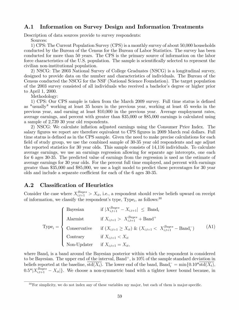
A.1 Information on Survey Design and Information TreatmentsDescription of data sources provide to survey respondents:Sources:1) CPS: The Current Population Survey (CPS) is a monthly survey of about 50,000 households

conducted by the Bureau of the Census for the Bureau of Labor Statistics. The survey has beenconducted for more than 50 years. The CPS is the primary source of information on the laborforce characteristics of the U.S. population. The sample is scienti�cally selected to represent thecivilian non-institutional population.2) NSCG: The 2003 National Survey of College Graduates (NSCG) is a longitudinal survey,

designed to provide data on the number and characteristics of individuals. The Bureau of theCensus conducted the NSCG for the NSF (National Science Foundation). The target populationof the 2003 survey consisted of all individuals who received a bachelor�s degree or higher priorto April 1, 2000.Methodology:1) CPS: Our CPS sample is taken from the March 2009 survey. Full time status is de�ned

as "usually" working at least 35 hours in the previous year, working at least 45 weeks in theprevious year, and earning at least $10,000 in the previous year. Average employment rates,average earnings, and percent with greater than $35,000 or $85,000 earnings is calculated usinga sample of 2,739 30 year old respondents.2) NSCG: We calculate in�ation adjusted earnings using the Consumer Price Index. The

salary �gures we report are therefore equivalent to CPS �gures in 2009 March real dollars. Fulltime status is de�ned as in the CPS sample. Given the need to make precise calculations for each�eld of study group, we use the combined sample of 30-35 year old respondents and age adjustthe reported statistics for 30 year olds. This sample consists of 14,116 individuals. To calculateaverage earnings, we use an earnings regression allowing for separate age intercepts, one eachfor 6 ages 30-35. The predicted value of earnings from the regression is used as the estimate ofaverage earnings for 30 year olds. For the percent full time employed, and percent with earningsgreater than $35,000 and $85,000, we use a logit model to predict these percentages for 30 yearolds and include a separate coe¢ cient for each of the 6 ages 30-35.

A.2 Classi�cation of HeuristicsConsider the case where XBayes

i;t+1 > Xit, i.e., a respondent should revise beliefs upward on receiptof information, we classify the respondent�s type, Typei, as follows:30

Typei =

8>>>>>>>><>>>>>>>>:

Bayesian if jXBayesi;t+1 �Xi;t+1j � Bandi

Alarmist if Xi;t+1 > XBayesi;t+1 + Band+

Conservative if (Xi;t+1 � Xit) & (Xi;t+1 < XBayesi;t+1 � Band�i )

Contrary if Xi;t+1 < Xit

Non-Updater if Xi;t+1 = Xit;

(A1)

where Bandi is a band around the Bayesian posterior within which the respondent is consideredto be Bayesian. The upper end of the interval, Band+, is 10% of the sample standard deviation inbeliefs reported at the baseline, std(Xt). The lower end of the band, Band�i = minf0.10*std(Xt);

0.5*jXBayesi;t+1 � Xitjg. We choose a non-symmetric band with a tighter lower bound because, in

30For simplicity, we do not index any of these variables my major, but each of them is major-speci�c.

59

cases where the sample standard deviation in beliefs is very large, we may be left with no conser-vative types. This criteria ensures that there are always some respondents who are classi�ed asconservatives. For downward revisions, the updating type is de�ned analogously. This classi�ca-tion, obviously, involves some subjectivity in how the band is de�ned. An alternative criteria thatinvolves no subjectivity is to classify any insu¢ cient (excessive) response relative to the Bayesianbenchmark as conservative (alarmist). Reducing the bandwidth around the Bayesian benchmarkto zero would ensure that almost all of the sample is classi�ed as non-Bayesian updaters.

A.3 Measurement Error in Self BeliefsIn order to understand the extent to which measurement error plague these data, we use data onrevisions of the control group. Recall, that for the control group, we elicited their self beliefs andpopulation beliefs in the initial stage, just as we did for the treatment group. However, in theintermediate stage, we re-elicited their self beliefs without providing any new information. Thenthe intermediate - initial beliefs for the Control group inform us about the extent of measurementerror in self earnings beliefs.Now consider the simple linear model:

yi = �x�i + "i;

where x�i is the true change in earnings beliefs for respondent i, and yi is say, the change inreported major probabilities. While x�i is unobserved, a measurement of xi of x

�i is observed

with:xi = x

�i + vi;

where vi is measurement error, and E(x�i vi) = 0. For the control group, since there is no changein actual earnings beliefs with no information provided, true revisions should be zero and soreported changes should be measurement error, i.e., xcontroli = vi. The probability limit of theleast squares estimator of � is:

plim b� = �(1� V ar(vi)

V ar(x�i ) + V ar(vi)) = ��;

where � is the reliability ratio, and equals V ar(x�i )V ar(x�i )+V ar(vi)

= V ar(xi)�V ar(vi)V ar(xi)

= 1 � V ar(vi)V ar(xi)

. Asmentioned above, V ar(xi) is obtained from the data on revisions of the treatment group, whileV ar(vi) which equals V ar(xcontroli ) is obtained from the revisions of the control group. The datayield a reliability ratio of 0.984, which indicates that measurement error is not a concern in thedata.

60