how did the first stars and galaxies form? abraham …loeb/photos/loeb.pdfhow did the first stars...
TRANSCRIPT
How Did the First Stars andGalaxies Form?
Abraham Loeb
PRINCETON UNIVERSITY PRESS
PRINCETON AND OXFORD

To my parents, Sara and David, who gave me life, and my three women,Ofrit, Klil and Lotem, who made it worthwhile
Contents
Preface v
Chapter 1. Prologue: The Big Picture 1
1.1 In the Beginning 11.2 Observing the Story of Genesis 11.3 Practical Benefits from the Big Picture 3
Chapter 2. Standard Cosmological Model 5
2.1 Cosmic Perspective 52.2 Past and Future of Our Universe 62.3 Gravitational Instability 82.4 Geometry of Space 82.5 Cosmic Archaeology 102.6 Milestones in Cosmic Evolution 132.7 Most Matter is Dark 17
Chapter 3. The First Gas Clouds 21
3.1 Growing the Seed Fluctuations 213.2 The Smallest Gas Condensations 243.3 Spherical Collapse and Halo Properties 263.4 Abundance of Dark Matter Halos 293.5 Cooling and Chemistry 333.6 Sheets, Filaments, and Only Then, Galaxies 35
Chapter 4. The First Stars and Black Holes 37
4.1 Metal-Free Stars 374.2 Properties of the First Stars 424.3 The First Black Holes and Quasars 444.4 Gamma-Ray Bursts: The Brightest Explosions 51
Chapter 5. The Reionization of Cosmic Hydrogen by the First Galaxies 55
5.1 Ionization Scars by the First Stars 555.2 Propagation of Ionization Fronts 565.3 Swiss Cheese Topology 62
Chapter 6. Observing the First Galaxies 67
6.1 Theories and Observations 676.2 Completing Our Photo Album of the Universe 67
iv CONTENTS
6.3 Cosmic Time Machine 696.4 The Hubble Deep Field and its Follow-ups 716.5 Observing the First Gamma-Ray Bursts 746.6 Future Telescopes 75
Chapter 7. Imaging the Diffuse Fog of Cosmic Hydrogen 79
7.1 Hydrogen 797.2 The Lyman-α Line 797.3 The 21-cm Line 817.4 Observing Most of the Observable Volume 91
Chapter 8. Epilogue: From Our Galaxy’s Past to Its Future 93
8.1 End of Extragalactic Astronomy 938.2 Milky Way+ Andromeda= Milkomeda 97
Appendix A. 101
Appendix B. Recommended Further Reading 105
Appendix C. Useful Numbers 107
Appendix D. Glossary 109
Index 113
Preface
This book captures the latest exciting developments concerning one of the un-solved mysteries about our origins:how did the first stars and galaxies light up inan expanding Universe that was on its way to becoming dark andlifeless?I sum-marize the fundamental principles and scientific ideas thatare being used to addressthis question, from the perspective of my own work over the past two decades.
Most research on this question has been theoretical so far. But the next few yearswill bring about a new generation of large telescopes with unprecedented sensi-tivity that promise to supply a flood of data about the infant Universe during itsfirst billion years after the Big Bang. Among the new observatories are the JamesWebb Space Telescope (JWST) – the successor to the Hubble Space Telescope,and three extremely large telescopes on the ground (rangingfrom 24 to 42 metersin diameter), as well as several new arrays of dipole antennae operating at low radiofrequencies. The fresh data on the first galaxies and the diffuse gas in between themwill test existing theoretical ideas about the formation and radiative effects of thefirst galaxies, and might even reveal new physics that has notyet been anticipated.This emerging interface between theory and observation will constitute an ideal op-portunity for students considering a research career in astrophysics or cosmology.With this in mind, the book is intended to provide a self-contained introduction toresearch on the first galaxies at a level appropriate for an undergraduate sciencemajor or a scientist with non-specialist background. Many of the non-technicalchapters are also suitable for the educated general public.
Various elements of the book are based on a cosmology class I have taught overthe past decade in the Astronomy and Physics departments at Harvard University.Other parts relate to overviews I wrote over the past decade in the form of fivereview articles (three with Rennan Barkana) and five popular-level articles (onewith Avery Broderick and one with TJ Cox). Where necessary, selected referencesare given to advanced papers and other review articles in thescientific literature.
The writing of this book was made possible thanks to the help Ireceived froma large number of people. First and foremost, I am grateful tomy parents, Saraand David, who supported my journey through life with unconditional love and un-derstanding. I also thank the many graduate students and senior collaborators withwhom I had fun learning about the contents of this book, including Dan Babich,John Bahcall, Rennan Barkana, Laura Blecha, Avery Broderick, Volker Bromm,Renyue Cen, Benedetta Ciardi, Mark Dijkstra, Daniel Eisenstein, Claude-AndreFaucher-Giguere, Richard Ellis, Steve Furlanetto, Zoltan Haiman, Lars Hernquist,Loren Hoffman, Bence Kocsis, Shri Kulkarni, Piero Madau, Joey Munoz, RameshNarayan, Ryan O’Leary, Jerry Ostriker, Jim Peebles, Rosalba Perna, Jonathan
vi PREFACE
Pritchard, Fred Rasio, Martin Rees, George Rybicki, Dan Stark, Max Tegmark,Anne Thoul, Hy Trac, Ed Turner, Eli Visbal, Eli Waxman, Stuart Wyithe and Ma-tias Zaldarriaga. Special thanks go to Claude-Andre Faucher-Giguere, Joey Munoz,Tony Pan, Jonathan Pritchard and Greg White for their careful reading of the bookand detailed comments, to Joey Munoz and Hy Trac for their help with severalfigures, and to Donna Adams for her assistance with the LaTex file and the illustra-tions. Finally, I would like to particularly thank the love of my life, Ofrit Liviatan,who established the foundations on which I stood while writing this book, and ourtwo daughters, Klil and Lotem, who inspired my thoughts about the future.
–A. L. Lexington MA, 2009
Chapter One
Prologue: The Big Picture
1.1 IN THE BEGINNING
As the Universe expands, galaxies get separated from one another, and the averagedensity of matter over a large volume of space is reduced. If we imagine playingthe cosmic movie in reverse and tracing this evolution backwards in time, we wouldinfer that there must have been an instant when the density ofmatter was infinite.This moment in time is the “ Big Bang”, before which we cannot reliably extrap-olate our history. But even before we get all the way back to the Big Bang, theremust have been a time when stars like our Sun and galaxies likeour Milky Wayi
did not exist, because the Universe was denser than they are.If so, how and whendid the first stars and galaxies form?
Primitive versions of this question were considered by humans for thousandsof years, long before it was realized that the Universe expands. Religious andphilosophical texts attempted to provide a sketch of the bigpicture from whichpeople could derive the answer. In retrospect, these attempts appear heroic in viewof the scarcity of scientific data about the Universe prior tothe twentieth century.To appreciate the progress made over the past century, consider, for example, thebiblical story of Genesis. The opening chapter of the Bible asserts the followingsequence of events: first, the Universe was created, then light was separated fromdarkness, water was separated from the sky, continents wereseparated from water,vegetation appeared spontaneously, stars formed, life emerged, and finally humansappeared on the scene.ii Instead, the modern scientific order of events begins withthe Big Bang, followed by an early period in which light (radiation) dominatedand then a longer period dominated by matter, leading to the appearance of stars,planets, life on Earth, and eventually humans. Interestingly, the starting and endpoints of both versions are the same.
1.2 OBSERVING THE STORY OF GENESIS
Cosmology is by now a mature empirical science. We are privileged to live in atime when the story of genesis (how the Universe started and developed) can be
iA star is a dense, hot ball of gas held together by gravity and powered by nuclear fusion reactions.A galaxy consists of a luminous core made of stars or cold gas surrounded by an extended halo ofdarkmatter(see§2.7).
ii Of course, it is possible to interpret the biblical text in many possible ways. Here I focus on a plainreading of the original Hebrew text.
2 CHAPTER 1
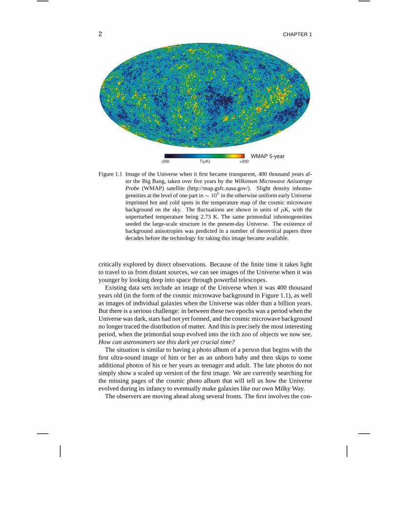
Figure 1.1 Image of the Universe when it first became transparent, 400 thousand years af-ter the Big Bang, taken over five years by theWilkinson Microwave AnisotropyProbe (WMAP) satellite (http://map.gsfc.nasa.gov/). Slight density inhomo-geneities at the level of one part in∼ 105 in the otherwise uniform early Universeimprinted hot and cold spots in the temperature map of the cosmic microwavebackground on the sky. The fluctuations are shown in units ofµK, with theunperturbed temperature being 2.73 K. The same primordial inhomogeneitiesseeded the large-scale structure in the present-day Universe. The existence ofbackground anisotropies was predicted in a number of theoretical papers threedecades before the technology for taking this image became available.
critically explored by direct observations. Because of thefinite time it takes lightto travel to us from distant sources, we can see images of the Universe when it wasyounger by looking deep into space through powerful telescopes.
Existing data sets include an image of the Universe when it was 400 thousandyears old (in the form of the cosmic microwave background in Figure 1.1), as wellas images of individual galaxies when the Universe was olderthan a billion years.But there is a serious challenge: in between these two epochswas a period when theUniverse was dark, stars had not yet formed, and the cosmic microwave backgroundno longer traced the distribution of matter. And this is precisely the most interestingperiod, when the primordial soup evolved into the rich zoo ofobjects we now see.How can astronomers see this dark yet crucial time?
The situation is similar to having a photo album of a person that begins with thefirst ultra-sound image of him or her as an unborn baby and thenskips to someadditional photos of his or her years as teenager and adult. The late photos do notsimply show a scaled up version of the first image. We are currently searching forthe missing pages of the cosmic photo album that will tell us how the Universeevolved during its infancy to eventually make galaxies likeour own Milky Way.
The observers are moving ahead along several fronts. The first involves the con-
PROLOGUE: THE BIG PICTURE 3
struction of large infrared telescopes on the ground and in space that will provideus with new (although rather expensive!) photos of galaxiesin the Universe at in-termediate ages. Current plans include ground-based telescopes which are 24-42meter in diameter, and NASA’s successor to the Hubble Space Telescope, the JamesWebb Space Telescope. In addition, several observational groups around the globeare constructing radio arrays that will be capable of mapping the three-dimensionaldistribution of cosmic hydrogen left over from the Big Bang in the infant Universe.These arrays are aiming to detect the long-wavelength (redshifted 21-cm) radioemission from hydrogen atoms. Coincidentally, this long wavelength (or low fre-quency) overlaps with the band used for radio and televisionbroadcasting, and sothese telescopes include arrays of regular radio antennas that one can find in elec-tronics stores. These antennas will reveal how the clumpy distribution of neutralhydrogen evolved with cosmic time. By the time the Universe was a few hundredsof millions of years old, the hydrogen distribution had beenpunched with holes likeswiss cheese. These holes were created by the ultraviolet radiation from the firstgalaxies and black holes, which ionized the cosmic hydrogenin their vicinity.
Theoretical research has focused in recent years on predicting the signals ex-pected from the above instruments and on providing motivation for these ambitiousobservational projects. In the subsequent chapters of thisbook, I will describe thetheoretical predictions as well as the observational programs planned for testingthem. Scientists operate similarly to detectives: they steadily revise their under-standing as they collect new information until their model appears consistent withall existing evidence. Their work is exciting as long as it isincomplete.
At a young age I was attracted to philosophy because it addresses the most fun-damental questions we face in life. As I matured to an adult, Irealized that sciencehas the benefit of formulating a subset of those questions that we can answer andmake steady progress on, using experimental evidence as a guide.
1.3 PRACTICAL BENEFITS FROM THE BIG PICTURE
I get paid to think about the sky. One might naively regard such an occupationas carrying no practical significance. If an engineer underestimates the strain on abridge, the bridge may collapse and harm innocent people. But if I calculate incor-rectly the evolution of galaxies, these mistakes bear no immediate consequence forthe daily life of other people.Is this really the case?
The same engineer who designs bridges would be the first to correct this naivemisconception. Newton arrived at his fundamental laws by studying the motion ofplanets around the Sun, and these laws are now used to build bridges and manyother products. Einstein’s general theory of relativity was developed to describethe cosmos but is also essential for achieving the required precision in modernnavigation or Global Positioning Systems (GPS) used for both civil and militaryapplications.
But there is a bigger context to the significance of the study of the Universe,namely, cosmology. The big picture gives us the practical advantage of having amore informed view of reality. Consider the weather, for example. It is a natural
4 CHAPTER 1
tendency for people to complain about the harsh weather in particular locations orseasons when rain or snow are common. Some might even associate the weatherpatterns with a divine entity that reacts to human actions. But if one observes anaerial photo from a satellite, it is easy to understand the origins of the weatherpatterns in particular locations. The data can be fed into a computer simulationthat uses the laws of physics to forecast the weather in advance. With a globalunderstanding of weather and climate patterns one obtains abetter sense of reality.
The biggest view we can have is that of the entire Universe. Inorder to have abalanced world-view we must understand the Universe. When Ilook up into thedark clear sky at night from the porch of my home in the town of Lexington, Mas-sachusetts, I wonder whether we humans are too often preoccupied with ourselves.There is much more to the Universe than meets the eye around uson Earth.
Chapter Two
Standard Cosmological Model
2.1 COSMIC PERSPECTIVE
In 1915 Einstein came up with the general theory of relativity. He was inspired bythe fact that all objects follow the same trajectories underthe influence of gravity(the so-called “equivalence principle,” which by now has been tested to better thanone part in a trillion), and realized that this would be a natural result if space-timeis curved under the influence of matter. He wrote down an equation describing howthe distribution of matter (on one side of his equation) determines the curvatureof space-time (on the other side of his equation). He then applied his equation todescribe the global dynamics of the Universe.
Back in 1915 there were no computers available, and Einstein’s equations for theUniverse were particularly difficult to solve in the most general case. It was there-fore necessary for Einstein to alleviate this difficulty by considering the simplestpossible Universe, one that is homogeneous and isotropic. Homogeneity meansuniform conditions everywhere (at any given time), and isotropy means the sameconditions in all directions when looking out from one vantage point. The combina-tion of these two simplifying assumptions is known as thecosmological principle.
The universe can be homogeneous but not isotropic: for example, the expansionrate could vary with direction. It can also be isotropic and not homogeneous: forexample, we could be at the center of a spherically-symmetric mass distribution.But if it is isotropic aroundeverypoint, then it must also be homogeneous.
Under the simplifying assumptions associated with the cosmological principle,Einstein and his contemporaries were able to solve the equations. They were look-ing for their “lost keys” (solutions) under the “lamppost” (simplifying assump-tions), but the real Universe is not bound by any contract to be the simplest that wecan imagine. In fact, it is truly remarkable in the first placethat we dare describethe conditions across vast regions of space based on the blueprint of the laws ofphysics that describe the conditions here on Earth. Our daily life teaches us toooften that we fail to appreciate complexity, and that an elegant model for reality isoften too idealized for describing the truth (along the lines of approximating a cowas a spherical object).
Back in 1915 Einstein had the wrong notion of the Universe; atthe time peopleassociated the Universe with the Milky Way galaxy and regarded all the “nebulae,”which we now know are distant galaxies, as constituents within our own MilkyWay galaxy. Because the Milky Way is not expanding, Einsteinattempted to re-produce a static universe with his equations. This turned out to be possible afteradding a cosmological constant, whose negative gravity would exactly counteract
6 CHAPTER 2
that of matter. However, he soon realized that this solutionis unstable: a slightenhancement in density would make the density grow even further. As it turns out,there are no stable static solution to Einstein’s equationsfor a homogenous andisotropic Universe. The Universe must either be expanding or contracting. Lessthan a decade later, Edwin Hubble discovered that the nebulae previously consid-ered to be constituents of the Milky Way galaxy are receding away from us at aspeedv that is proportional to their distancer, namelyv = H0r with H0 a spatialconstant (which could evolve with time), commonly termed the Hubble constant.Hubble’s data indicated that the Universe is expanding.
Einstein was remarkably successful in asserting the cosmological principle. Asit turns out, our latest data indicates that the real Universe is homogeneous andisotropic on the largest observable scales to within one part in a hundred thousand.Fortuitously, Einstein’s simplifying assumptions turnedout to be extremely accu-rate in describing reality:the keys were indeed lying next to the lamppost. OurUniverse happens to be the simplest we could have imagined, for which Einstein’sequations can be easily solved.
Why was the Universe prepared to be in this special state?Cosmologists wereable to go one step further and demonstrate that an early phase transition, calledcosmic inflation – during which the expansion of the Universe accelerated expo-nentially, could have naturally produced the conditions postulated by the cosmo-logical principle. One is left to wonder whether the existence of inflation is just afortunate consequence of the fundamental laws of nature, orwhether perhaps thespecial conditions of the specific region of space-time we inhabit were selectedout of many random possibilities elsewhere by the prerequisite that they allow ourexistence. The opinions of cosmologists on this question are split.
2.2 PAST AND FUTURE OF OUR UNIVERSE
Hubble’s discovery of the expansion of the Universe has immediate implicationswith respect to the past and future of the Universe. If we reverse in our mind theexpansion history back in time, we realize that the Universemust have been denserin its past. In fact, there must have been a point in time wherethe matter densitywas infinite, at the moment of the so-called Big Bang. Indeed we do detect relicsfrom a hotter denser phase of the Universe in the form of lightelements (suchas deuterium, helium and lithium) as well as the Cosmic Microwave Background(CMB). At early times, this radiation coupled extremely well to the cosmic gasand obtained a spectrum known as blackbody, that was predicted a century agoto characterize matter and radiation in equilibrium. The CMB provides the bestexample of a blackbody spectrum we have.
To get a rough estimate of when the Big Bang occurred, we may simply dividethe distance of all galaxies by their recession velocity. This gives a unique answer,∼ r/v ∼ 1/H0, which is independent of distance.i The latest measurements of the
iAlthough this is an approximate estimate, it turns out to be within a few percent of the true ageof our Universe owing to a coincidence. The cosmic expansionat first decelerated and then accelerated
STANDARD COSMOLOGICAL MODEL 7
Hubble constant give a value ofH0 ≈ 70 kilometers per second per Megaparsec,ii
implying a current age for the Universe1/H0 of 14 billion years (or5 × 1017
seconds).The second implication concerns our future. A fortunate feature of a spherically-
symmetric Universe is that when considering a sphere of matter in it, we are al-lowed to ignore the gravitational influence of everything outside this sphere. If weempty the sphere and consider a test particle on the boundaryof an empty voidembedded in a uniform Universe, the particle will experience no net gravitationalacceleration. This result, known as Birkhoff’s theorem, isreminiscent of Newton’s“iron sphere theorem.” It allows us to solve the equations ofmotion for matter onthe boundary of the sphere through a local analysis without worrying about the restof the Universe. Therefore, if the sphere has exactly the same conditions as the restof the Universe, we may deduce the global expansion history of the Universe byexamining its behavior. If the sphere is slightly denser than the mean, we will inferhow its density contrast will evolve relative to the background Universe.
The equation describing the motion of a spherical shell of matter is identical tothe equation of motion of a rocket launched from the surface of the Earth. Therocket will escape to infinity if its kinetic energy exceeds its gravitational bindingenergy, making its total energy positive. However, if its total energy is negative,the rocket will reach a maximum height and then fall back. In order to figure outthe future evolution of the Universe, we need to examine the energy of a sphericalshell of matter relative to the origin. With a uniform density ρ, a spherical shellof radiusr would have a total massM = ρ ×
(
4π3 r3
)
enclosed within it. Itsenergy per unit mass is the sum of the kinetic energy due to itsexpansion speedv = Hr, 1
2v2, and its potential gravitational energy,−GM/r (whereG is Newton’sconstant), namelyE = 1
2v2 − GMr . By substituting the above relations forv and
M , it can be easily shown thatE = 12v2(1 − Ω), whereΩ = ρ/ρc andρc =
3H2/8πG is defined as thecritical density. We therefore find that there are threepossible scenarios for the cosmic expansion. The Universe has either:(i) Ω >1, making it gravitationally bound withE < 0 – such a “closed Universe” willturn-around and end up collapsing towards a “big crunch”; (ii) Ω < 1, makingit gravitationally unbound withE > 0 – such an “open Universe” will expandforever; or the borderline case(iii) Ω = 1, making the Universe marginally boundor “flat” with E = 0.
Einstein’s equations relate the geometry of space to its matter content throughthe value ofΩ: an open Universe has a geometry of a saddle with a negative spatialcurvature, a closed Universe has the geometry of a sphericalglobe with a positivecurvature, and a flat Universe has a flat geometry with no curvature. Our observablesection of the Universe appears to be flat.
with the two almost canceling each other out at the present-time, giving the same age as if the expansionwere at a constant speed (as would be strictly true only in an empty Universe).
ii A megaparsec (abbreviated as ‘Mpc’) is equivalent to3.086 × 1024 centimeter, or roughly thedistance traveled by light in three million years.
8 CHAPTER 2
2.3 GRAVITATIONAL INSTABILITY
Now we are at a position to understand how objects, like the Milky Way galaxy,have formed out of small density inhomogeneities that get amplified by gravity.
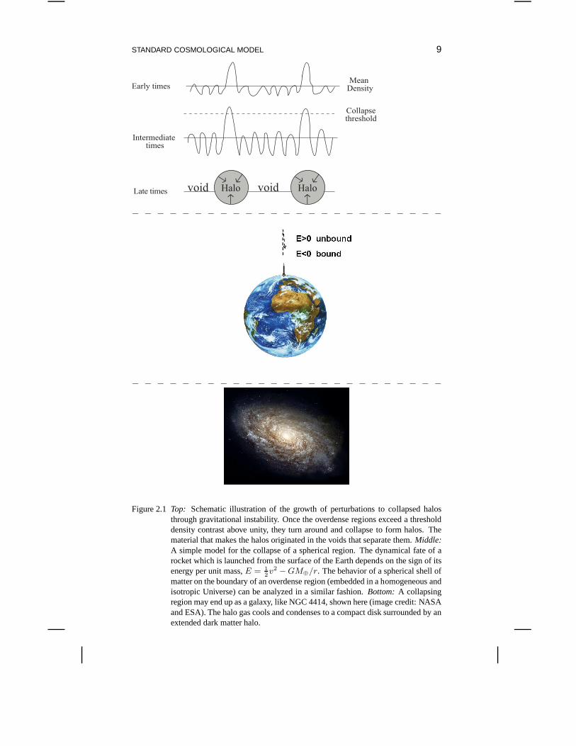
Let us consider for simplicity the background of a marginally bound (flat) Uni-verse which is dominated by matter. In such a background, only a slight en-hancement in density is required for exceeding the criticaldensityρc. Becauseof Birkhoff’s theorem, a spherical region that is denser than the mean will behaveas if it is part of a closed Universe and increase its density contrast with time, whilean underdense spherical region will behave as if it is part ofan open Universe andappear more vacant with time relative to the background, as illustrated in Figure2.1. Starting with slight density enhancements that bring them above the criticalvalueρc, the overdense regions will initially expand, reach a maximum radius, andthen collapse upon themselves (like the trajectory of a rocket launched straight up,away from the center of the Earth). An initially slightly inhomogeneous Universewill end up clumpy, with collapsed objects forming out of overdense regions. Thematerial to make the objects is drained out of the intervening underdense regions,which end up as voids.
The Universe we live in started with primordial density perturbations of a frac-tional amplitude∼ 10−5. The overdensities were amplified at late times (oncematter dominated the cosmic mass budget) up to values close to unity and col-lapsed to make objects, first on small scales. We have not yet seen the first smallgalaxies that started the process that eventually led to theformation of big galaxieslike the Milky Way. The search for the first galaxies is a search for our origins.
Life as we know it on planet Earth requires water. The water molecule includesoxygen, an element that was not made in the Big Bang and did notexist until thefirst stars had formed. Therefore our form of life could not have existed in thefirst hundred millions of years after the Big Bang, before thefirst stars had formed.There is also no guarantee that life will persist in the distant future.
2.4 GEOMETRY OF SPACE
How can we tell the difference between the flat surface of a book and the curvedsurface of a balloon?A simple way would be to draw a triangle of straight linesbetween three points on those surfaces and measure the sum ofthe three anglesof the triangle. The Greek mathematician Euclid demonstrated that the sum ofthese angles must be 180 degrees (orπ radians) on a flat surface. Twenty-onecenturies later, the German mathematician Bernhard Riemann extended the field ofgeometry to curved spaces, which played an important role inthe development ofEinstein’s general theory of relativity. For a triangle drawn on a positively curvedsurface, like that of a balloon, the sum of the angles is larger than 180 degrees.(This can be easily figured out by examining a globe and noticing that any lineconnecting one of the poles to the equator opens an angle of 90degrees relative tothe equator. Adding the third angle in any triangle stretched between the pole andthe equator would surely result in a total of more than 180 degrees.) According to
STANDARD COSMOLOGICAL MODEL 9
Early timesMean
Density
Intermediate times
Late times
Collapsethreshold
void voidHalo Halo
− − − − − − − − − − − − − − − − − − − − − − − − −
− − − − − − − − − − − − − − − − − − − − − − − − −
Figure 2.1 Top: Schematic illustration of the growth of perturbations to collapsed halosthrough gravitational instability. Once the overdense regions exceed a thresholddensity contrast above unity, they turn around and collapseto form halos. Thematerial that makes the halos originated in the voids that separate them.Middle:A simple model for the collapse of a spherical region. The dynamical fate of arocket which is launched from the surface of the Earth depends on the sign of itsenergy per unit mass,E = 1
2v2 − GM⊕/r. The behavior of a spherical shell of
matter on the boundary of an overdense region (embedded in a homogeneous andisotropic Universe) can be analyzed in a similar fashion.Bottom: A collapsingregion may end up as a galaxy, like NGC 4414, shown here (imagecredit: NASAand ESA). The halo gas cools and condenses to a compact disk surrounded by anextended dark matter halo.
10 CHAPTER 2
Einstein’s equations, the geometry of the Universe is dictated by its matter content;in particular, the Universe is flat only if the totalΩ equals unity.Is it possible todraw a triangle across the entire Universe and measure its geometry?
Remarkably, the answer isyes. At the end of the twentieth century cosmologistswere able to perform this experiment1 by adopting a simple yardstick provided bythe early Universe. The familiar experience of dropping a stone in the middle ofa pond results in a circular wave crest that propagates outwards. Similarly, per-turbing the smooth Universe at a single point at the Big Bang would have resultedin a spherical sound wave propagating out from that point. The wave would havetraveled at the speed of sound, which was of order the speed oflight c (or moreprecisely, 1√
3c) early on when radiation dominated the cosmic mass budget. At any
given time, all the points extending to the distance traveled by the wave are affectedby the original pointlike perturbation. The conditions outside this “sound horizon”will remain uncorrelated with the central point, because acoustic information hasnot been able to reach them at that time. The temperature fluctuations of the CMBtrace the simple sum of many such pointlike perturbations that were generated inthe Big Bang. The patterns they delineate would therefore show a characteristiccorrelation scale, corresponding to the sound horizon at the time when the CMBwas produced, 400 thousand years after the Big Bang. By measuring the apparentangular scale of this “standard ruler” on the sky, known as the acoustic peak inthe CMB, and comparing it to theory, experimental cosmologists inferred from thesimple geometry of triangles that the Universe is flat.
The inferred flatness is a natural consequence of the early period of vast expan-sion, known as cosmic inflation, during which any initial curvature was flattened.Indeed a small patch of a fixed size (representing our currentobservable region inthe cosmological context) on the surface of a vastly inflatedballoon would appearnearly flat. The sum of the angles on a non-expanding triangleplaced on this patchwould get arbitrarily close to 180 degrees as the balloon inflates.
2.5 COSMIC ARCHAEOLOGY
Our Universe is the simplest possible on two counts: it satisfies the cosmologicalprinciple, and it has a flat geometry. The mathematical description of an expanding,homogeneous, and isotropic Universe with a flat geometry is straightforward. Wecan imagine filling up space with clocks that are all synchronized. At any givensnapshot in time the physical conditions (density, temperature) are the same every-where. But as time goes on, the spatial separation between the clocks will increase.The stretching of space can be described by a time-dependentscale factor,a(t).A separation measured at timet1 asr(t1) will appear at timet2 to have a lengthr(t2) = r(t1)[a(t2)/a(t1)].
A natural question to ask is whether our human bodies or even the solar system,are also expanding as the Universe expands. The answer is no,because these sys-tems are held together by forces whose strength far exceeds the cosmic force. Themean density of the Universe today,ρ, is 29 orders of magnitude smaller than the
STANDARD COSMOLOGICAL MODEL 11
density of our body. Not only are the electromagnetic forcesthat keep the atomsin our body together far greater than gravity, but even the gravitational self-forceof our body on itself overwhelms the cosmic influence. Only onvery large scalesdoes the cosmic gravitational force dominate the scene. This also implies that wecannot observe the cosmic expansion with a local laboratoryexperiment; in orderto notice the expansion we need to observe sources which are spread over the vastscales of millions of light years.
A source located at a separationr = a(t)x from us would move at a velocityv = dr/dt = ax = (a/a)r, wherea = da/dt. Herex is a time-independenttag, denoting the present-day distance of the source. Defining H = a/a which isconstant in space, we recover the Hubble expansion lawv = Hr.
Edwin Hubble measured the expansion of the Universe using the Doppler effect.We are all familiar with the same effect for sound waves: whena moving car soundsits horn, the pitch (frequency) we hear is different if the car is approaching us orreceding away. Similarly, the wavelength of light depends on the velocity of thesource relative to us. As the Universe expands, a light source will move awayfrom us and its Doppler effect will change with time. The Doppler formula for anearby source of light (with a recession speed much smaller than the speed of light)gives∆ν/ν ≈ −∆v/c = −(a/a)(r/c) = −(a∆t)/a = −∆a/a, admitting thesolutionν ∝ a−1. Correspondingly, the wavelength scales asλ = (c/ν) ∝ a. Wecould have anticipated this outcome since a wavelength can be used as a measure ofdistance and should therefore be stretched as the Universe expands. The redshiftzis defined through the factor(1+z) by which the photon wavelength was stretched(or its frequency reduced) between its emission and observation times. If we definea = 1 today, thena = 1/(1 + z) at earlier times. Higher redshifts correspond to ahigher recession speed of the source relative to us (ultimately approaching the speedof light when the redshift goes to infinity), which in turn implies a larger distance(ultimately approaching our horizon, which is the distancetraveled by light sincethe Big Bang) and an earlier emission time of the source in order for the photons toreach us today.
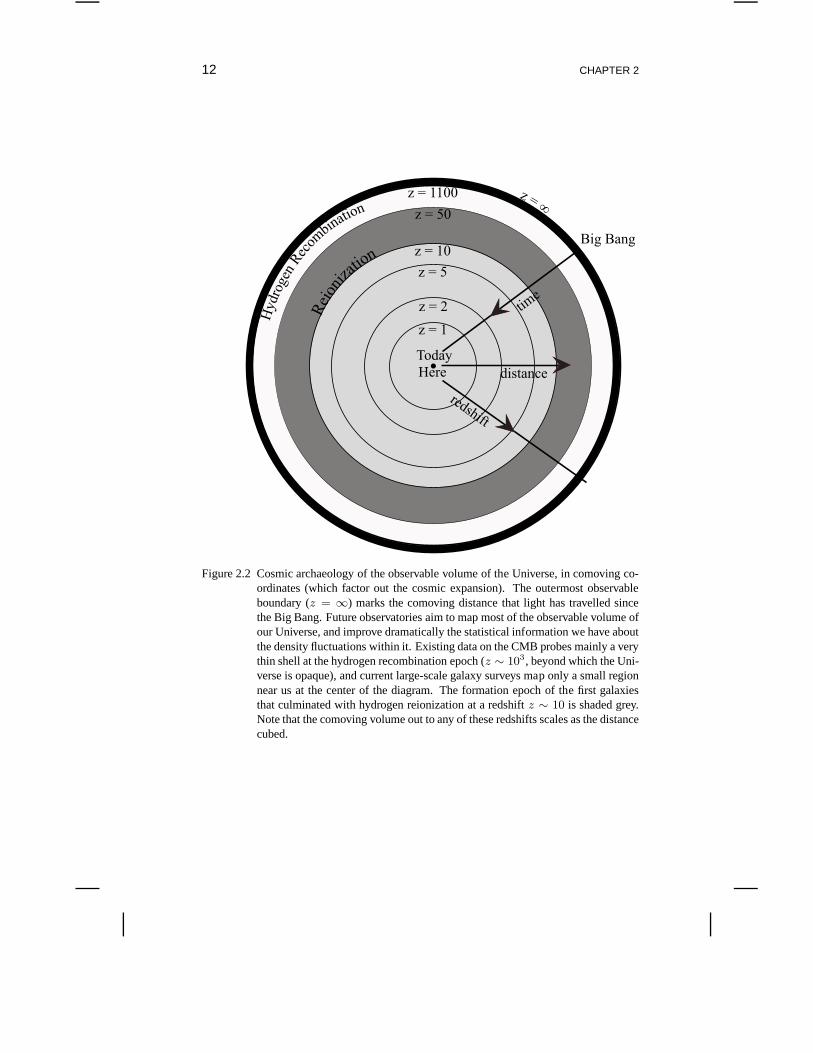
We see high-redshift sources as they looked at early cosmic times. Observationalcosmology is like archaeology – the deeper we look into spacethe more ancient theclues about our history are (see Figure 2.2). But there is a limit to how far back wecan see. In principle, we can image the Universe only as long as it was transparent,corresponding to redshiftsz < 103 for photons. The first galaxies are believed tohave formed long after that.
The expansion history of the Universe is captured by the scale factora(t). Wecan write a simple equation for the evolution ofa(t) based on the behavior of asmall region of space. For that purpose we need to incorporate the fact that inEinstein’s theory of gravity, not only does mass densityρ gravitate but pressurep does too. In a homogeneous and isotropic Universe, the quantity ρgrav = (ρ +3p/c2) plays the role of the gravitating mass densityρ of Newtonian gravity.2 Thereare several examples to consider. For a radiation fluid,iii prad/c2 = 1
3ρrad, implying
iii The momentum of each photon is1c
of its energy. The pressure is defined as the momentum flux
along one dimension out of three, and is therefore given by1
3ρradc2, whereρrad is the mass density of
12 CHAPTER 2
z = 1100
z = 50
z = 10
z = 1
z = 2
z = 5
Big Bang
Today
Here distance
time
redshift
Hydro
gen
Rec
ombinati
on
Rei
oniz
ation
z = ∞
Figure 2.2 Cosmic archaeology of the observable volume of the Universe, in comoving co-ordinates (which factor out the cosmic expansion). The outermost observableboundary (z = ∞) marks the comoving distance that light has travelled sincethe Big Bang. Future observatories aim to map most of the observable volume ofour Universe, and improve dramatically the statistical information we have aboutthe density fluctuations within it. Existing data on the CMB probes mainly a verythin shell at the hydrogen recombination epoch (z ∼ 103, beyond which the Uni-verse is opaque), and current large-scale galaxy surveys map only a small regionnear us at the center of the diagram. The formation epoch of the first galaxiesthat culminated with hydrogen reionization at a redshiftz ∼ 10 is shaded grey.Note that the comoving volume out to any of these redshifts scales as the distancecubed.
STANDARD COSMOLOGICAL MODEL 13
thatρgrav = 2ρrad. On the other hand, for a constant vacuum density (the so-called“cosmological constant”), the pressure is negative because by opening up a newvolume increment∆V one gains an energyρc2∆V instead of losing energy, asis the case for normal fluids that expand into more space. In thermodynamics,pressure is derived from the deficit in energy per unit of new volume, which in thiscase givespvac/c2 = −ρvac. This in turn leads to another reversal of signs,ρgrav =(ρvac + 3pvac/c2) = −2ρvac, which may be interpreted as repulsive gravity! Thissurprising result gives rise to the phenomenon of accelerated cosmic expansion,which characterized the early period of cosmic inflation as well as the latest sixbillions years of cosmic history.
As the Universe expands and the scale factor increases, the matter mass densitydeclines inversely with volume,ρmatter ∝ a−3, whereas the radiation energy den-sity decreases asρradc2 ∝ a−4, because not only is the density of photons dilutedasa−3, but the energy per photonhν = hc/λ (whereh is Planck’s constant) de-clines asa−1. Todayρmatter is larger thanρrad by a factor of∼ 3, 300, but at(1 + z) ∼ 3, 300 the two were equal, and at even higher redshifts the radiationdominated. Since a stable vacuum does not get diluted with cosmic expansion, thepresent-dayρvac remained a constant and dominated overρmatter andρrad only atlate times (whereas the unstable “false vacuum” that dominated during inflation hasdecayed when inflation ended).
2.6 MILESTONES IN COSMIC EVOLUTION
The gravitating mass,Mgrav = ρgravV , enclosed by a spherical shell of radiusa(t)and volumeV = 4π
3 a3, induces an acceleration
d2a
dt2= −GMgrav
a2. (2.1)
Sinceρgrav = ρ+3p/c2, we need to know how pressure evolves with the expansionfactor a(t). This is obtained from the thermodynamic relation mentioned abovebetween the change in the internal energyd(ρc2V ) and thepdV work done bythe pressure,d(ρc2V ) = −pdV . This relation implies−3paa/c2 = a2ρ + 3ρaa,where a dot denotes a time derivative. Multiplying equation(2.1) bya and makinguse of this relation yields our familiar result
E =1
2a2 − GM
a, (2.2)
whereE is a constant of integration andM ≡ ρV . As discussed before, the spher-ical shell will expand forever (being gravitationally unbound) if E ≥ 0, but willeventually collapse (being gravitationally bound) ifE < 0. Making use of theHubble parameter,H = a/a, equation (2.2) can be re-written as
E12 a2
= 1 − Ω, (2.3)
the radiation.
14 CHAPTER 2
whereΩ = ρ/ρc, with
ρc =3H2
8πG= 9.2 × 10⁻³⁰ g
cm3
(
H
70 km s−1Mpc−1
)2
. (2.4)
With Ωm, ΩΛ, andΩr denoting the present contributions toΩ from matter (includ-ing cold dark matter [see§2.7] as well as a contributionΩb from ordinary matter ofprotons and neutrons, or “baryons”), vacuum density (cosmological constant), andradiation, respectively, a flat universe satisfies
H(t)
H0=
[
Ωm
a3+ ΩΛ +
Ωr
a4
]1/2
, (2.5)
where we defineH0 andΩ0 = (Ωm + ΩΛ + Ωr) = 1 to be the present-day valuesof H andΩ, respectively.
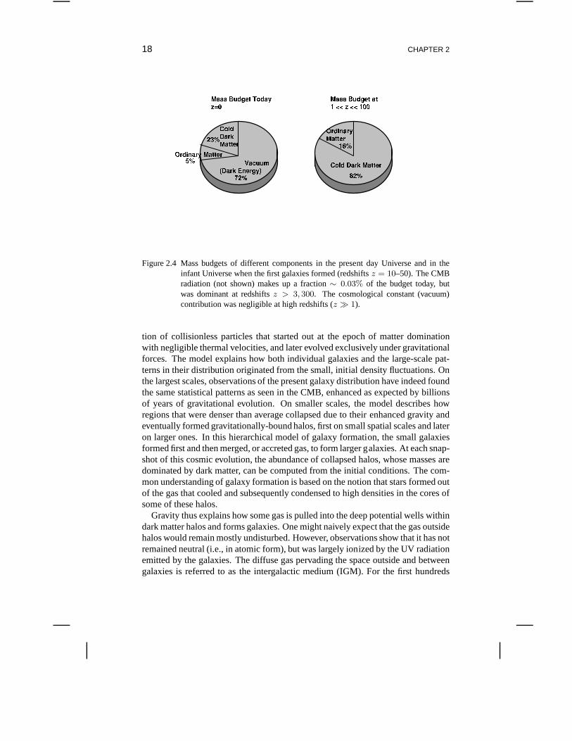
In the particularly simple case of a flat Universe, we find thatif matter dominatesthena ∝ t2/3, if radiation dominates thena ∝ t1/2, and if the vacuum densitydominates thena ∝ expHvact with Hvac = (8πGρvac/3)1/2 being a constant.In the beginning, after inflation ended, the mass density of our Universeρ was atfirst dominated by radiation at redshiftsz > 3, 300, then it became dominated bymatter at0.3 < z < 3, 300, and finally was dominated by the vacuum atz < 0.3.The vacuum started to dominateρgrav already atz < 0.7 or six billion years ago.Figure 2.4 illustrates the mass budget in the present-day Universe and during theepoch when the first galaxies had formed.
The above results fora(t) have two interesting implications. First, we can figureout the relationship between the time since the Big Bang and redshift sincea =(1 + z)−1. For example, during the matter-dominated era (1 < z < 103),
t ≈ 2
3H0Ωm1/2(1 + z)3/2
=0.95 × 10⁹ years
[(1 + z)/7]3/2. (2.6)
Second, we note the remarkable exponential expansion for a vacuum dominatedphase. This accelerated expansion serves an important purpose in explaining a fewpuzzling features of our Universe. We already noticed that our Universe was pre-pared in a very special initial state: nearly isotropic and homogeneous, withΩ closeto unity and a flat geometry. In fact, it took the CMB photons nearly the entire ageof the Universe to travel towards us. Therefore, it should take them twice as long tobridge across their points of origin on opposite sides of thesky. How is it possiblethen that the conditions of the Universe (as reflected in the nearly uniform CMBtemperature) were prepared to be the same in regions that were never in causalcontact before?Such a degree of organization is highly unlikely to occur at ran-dom. If we receive our clothes ironed out and folded neatly, we know that theremust have a been a process that caused it. Cosmologists have identified an analo-gous “ironing process” in the form ofcosmic inflation. This process is associatedwith an early period during which the Universe was dominatedtemporarily by themass density of an elevated vacuum state, and experienced exponential expansionby at least∼ 60 e-folds. This vast expansion “ironed out” any initial curvatureof our environment, and generated a flat geometry and nearly uniform conditionsacross a region far greater than our current horizon. After the elevated vacuum statedecayed, the Universe became dominated by radiation.
STANDARD COSMOLOGICAL MODEL 15
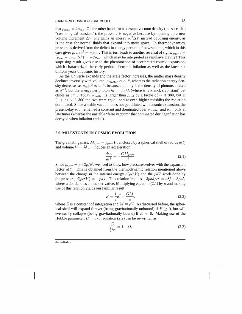
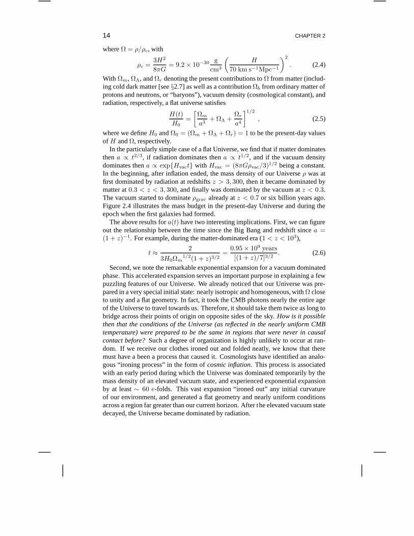
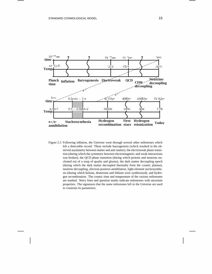
Figure 2.3 Following inflation, the Universe went through several other milestones whichleft a detectable record. These include baryogenesis (which resulted in the ob-served asymmetry between matter and anti-matter), the electroweak phase transi-tion (during which the symmetry between electromagnetic and weak interactionswas broken), the QCD phase transition (during which protonsand neutrons nu-cleated out of a soup of quarks and gluons), the dark matter decoupling epoch(during which the dark matter decoupled thermally from the cosmic plasma),neutrino decoupling, electron-positron annihilation, light-element nucleosynthe-sis (during which helium, deuterium and lithium were synthesized), and hydro-gen recombination. The cosmic time and temperature of the various milestonesare marked. Wavy lines and question marks indicate milestones with uncertainproperties. The signatures that the same milestones left inthe Universe are usedto constrain its parameters.
16 CHAPTER 2
The early epoch of inflation is important not just in producing the global prop-erties of the Universe but also in generating the inhomogeneities that seeded theformation of galaxies within it.3 The vacuum energy density that had driven in-flation encountered quantum mechanical fluctuations. Afterthe perturbations werestretched beyond the horizon of the infant Universe (which today would have oc-cupied the size no bigger than a human hand), they materialized as perturbations inthe mass density of radiation and matter. The last perturbations to leave the horizonduring inflation eventually entered back after inflation ended (when the scale factorgrew more slowly thanct). It is tantalizing to contemplate the notion that galaxies,which represent massive classical objects with∼ 1067 atoms in today’s Universe,might have originated from sub-atomic quantum-mechanicalfluctuations at earlytimes.
After inflation, an unknown process, called “baryo-genesis” or “lepto-genesis”,generated an excess of particles (baryons and leptons) overanti-particles.iv Asthe Universe cooled to a temperature of hundreds of MeV (with1MeV/kB =1.1604 × 10¹⁰K), protons and neutrons condensed out of the primordial quark-gluon plasma through the so-calledQCD phase transition. At about one secondafter the Big Bang, the temperature declined to∼ 1 MeV, and the weakly interact-ing neutrinos decoupled. Shortly afterwards the abundanceof neutrons relative toprotons froze and electrons and positrons annihilated. In the next few minutes, nu-clear fusion reactions produced light elements more massive than hydrogen, suchas deuterium, helium, and lithium, in abundances that matchthose observed todayin regions where gas has not been processed subsequently through stellar interi-ors. Although the transition to matter domination occurredat a redshiftz ∼ 3, 300the Universe remained hot enough for the gas to be ionized, and electron-photonscattering effectively coupled ordinary matter and radiation. At z ∼ 1, 100 thetemperature dipped below∼ 3, 000K, and free electrons recombined with protonsto form neutral hydrogen atoms. As soon as the dense fog of free electrons was de-pleted, the Universe became transparent to the relic radiation, which is observed atpresent as the CMB. These milestones of the thermal history are depicted in Figure2.3.
The Big Bang is the only known event in our past history where particles in-teracted with center-of-mass energies approaching the so-called “Planck scale”v
[(hc5/G)1/2 ∼ 1019 GeV], at which quantum mechanics and gravity are expectedto be unified. Unfortunately, the exponential expansion of the Universe during in-flation erased memory of earlier cosmic epochs, such as the Planck time.
ivAnti-particles are identical to particles but with opposite electric charge. Today, the ordinarymatter in the Universe is observed to consist almost entirely of particles. The origin of the asymmetryin the cosmic abundance of matter over anti-matter is stil anunresolved puzzle.
vThe Planck energy scale is obtained by equating the quantum-mechanical wavelength of a rela-tivistic particle with energyE, namelyhc/E, to its “black hole” radius∼ GE/c4, and solving forE.
STANDARD COSMOLOGICAL MODEL 17
2.7 MOST MATTER IS DARK
Surprisingly, most of the matter in the Universe is not the same ordinary matter thatwe are made of (see Figure 2.4). If it were ordinary matter (which also makes starsand diffuse gas), it would have interacted with light, thereby revealing its existenceto observations through telescopes. Instead, observations of many different astro-physical environments require the existence of some mysterious dark componentof matter which only reveals itself through its gravitational influence and leaves noother clue about its nature. Cosmologists are like a detective who finds evidencefor some unknown criminal in a crime scene and is anxious to find his/her identity.The evidence for dark matter is clear and indisputable, assuming that the laws ofgravity are not modified (although a small minority of scientists are exploring thisalternative).
Without dark matter we would have never existed by now. This is because or-dinary matter is coupled to the CMB radiation that filled up the Universe early on.The diffusion of photons on small scales smoothed out perturbations in this pri-mordial radiation fluid. The smoothing length was stretchedto a scale as large ashundreds of millions of light years in the present-day Universe. This is a huge scaleby local standards, since galaxies – like the Milky Way – wereassembled out ofmatter in regions a hundred times smaller than that. Becauseordinary matter wascoupled strongly to the radiation in the early dense phase ofthe Universe, it alsowas smoothed on small scales. If there was nothing else in addition to the radiationand ordinary matter, then this smoothing process would havehad a devastating ef-fect on the prospects for life in our Universe. Galaxies likethe Milky Way wouldhave never formed by the present time since there would have been no density per-turbations on the relevant small scales to seed their formation. The existence ofdark matter not coupled to the radiation came to the rescue bykeeping memoryof the initial seeds of density perturbations on small scales. In our neighborhood,these seed perturbations led eventually to the formation ofthe Milky Way galaxyinside of which the Sun was made as one out of tens of billions of stars, and theEarth was born out of the debris left over from the formation process of the Sun.This sequence of events would have never occurred without the dark matter.
We do not know what the dark matter is made of, but from the goodmatch ob-tained between observations of large-scale structure and the equations describing apressureless fluid (see equations 3.3-3.4), we infer that itis likely made of particleswith small random velocities. It is therefore called “cold dark matter” (CDM). Thepopular view is that CDM is composed of particles which possess weak interactionswith ordinary matter, similarly to the elusive neutrinos weknow to exist. The hopeis that CDM particles, owing to their weak but non-vanishingcoupling to ordinarymatter, will nevertheless be produced in small quantities through collisions of ener-getic particles in future laboratory experiments such as the Large Hadron Collider(LHC).4 Other experiments are attempting to detect directly the astrophysical CDMparticles in the Milky Way halo. A positive result from any ofthese experimentswill be equivalent to our detective friend being successfulin finding a DNA sampleof the previously unidentified criminal.
According to the standard cosmological model, the CDM behaves as a collec-
18 CHAPTER 2
Figure 2.4 Mass budgets of different components in the present day Universe and in theinfant Universe when the first galaxies formed (redshiftsz = 10–50). The CMBradiation (not shown) makes up a fraction∼ 0.03% of the budget today, butwas dominant at redshiftsz > 3, 300. The cosmological constant (vacuum)contribution was negligible at high redshifts (z ≫ 1).
tion of collisionless particles that started out at the epoch of matter dominationwith negligible thermal velocities, and later evolved exclusively under gravitationalforces. The model explains how both individual galaxies andthe large-scale pat-terns in their distribution originated from the small, initial density fluctuations. Onthe largest scales, observations of the present galaxy distribution have indeed foundthe same statistical patterns as seen in the CMB, enhanced asexpected by billionsof years of gravitational evolution. On smaller scales, themodel describes howregions that were denser than average collapsed due to theirenhanced gravity andeventually formed gravitationally-bound halos, first on small spatial scales and lateron larger ones. In this hierarchical model of galaxy formation, the small galaxiesformed first and then merged, or accreted gas, to form larger galaxies. At each snap-shot of this cosmic evolution, the abundance of collapsed halos, whose masses aredominated by dark matter, can be computed from the initial conditions. The com-mon understanding of galaxy formation is based on the notionthat stars formed outof the gas that cooled and subsequently condensed to high densities in the cores ofsome of these halos.
Gravity thus explains how some gas is pulled into the deep potential wells withindark matter halos and forms galaxies. One might naively expect that the gas outsidehalos would remain mostly undisturbed. However, observations show that it has notremained neutral (i.e., in atomic form), but was largely ionized by the UV radiationemitted by the galaxies. The diffuse gas pervading the spaceoutside and betweengalaxies is referred to as the intergalactic medium (IGM). For the first hundreds
STANDARD COSMOLOGICAL MODEL 19
of millions of years after cosmological recombination (when protons and electronscombined to make neutral hydrogen), the so-called cosmic “dark ages,” the universewas filled with diffuse atomic hydrogen. As soon as galaxies formed, they startedto ionize diffuse hydrogen in their vicinity. Within less than a billion years, mostof the IGM was reionized.

Chapter Three
The First Gas Clouds
The initial conditions of the Universe can be summarized on asingle sheet of paper.The small number of parameters that provide an accurate statistical description ofthese initial conditions are summarized in Table 3.1. However, thousands of booksin libraries throughout the world cannot summarize the complexities of galaxies,stars, planets, life, and intelligent life, in the present-day Universe. If we feed thesimple initial cosmic conditions into a gigantic computer simulation incorporat-ing the known laws of physics, we should be able to reproduce all the complexitythat emerged out of the simple early universe. Hence, all theinformation associ-ated with this later complexity was encapsulated in those simple initial conditions.Below we follow the process through which late time complexity appeared andestablished an irreversible arrow to the flow of cosmic time.i
After cosmological recombination, the Universe entered the “dark ages” duringwhich the relic CMB light from the Big Bang gradually faded away. During this“pregnancy” period which lasted hundreds of millions of years, the seeds of smalldensity fluctuations planted by inflation in the matter distribution grew up until theyeventually collapsed to make the first galaxies.5
3.1 GROWING THE SEED FLUCTUATIONS
As discussed earlier, small perturbations in density grow due to the unstable natureof gravity. Overdense regions behave as if they reside in a closed Universe. Theirevolution ends in a “big crunch”, which results in the formation of gravitationallybound objects like the Milky Way galaxy.
Equation (2.3) explains the formation of galaxies out of seed density fluctuationsin the early Universe, at a time when the mean matter density was very close to
Table 3.1 Standard set of cosmological parameters (defined and adopted throughout thebook). Based on Komatsu,E., et al.Astrophys. J. Suppl.180, 330 (2009).
ΩΛ Ωm Ωb h ns σ8
0.72 0.28 0.05 0.7 1 0.82
i In previous decades, astronomers used to associate the simplicity of the early Universe with thefact that the data about it was scarce. Although this was trueat the infancy of observational cosmology,it is not true any more. With much richer data in our hands, theinitial simplicity is now interpreted asan outcome of inflation.
22 CHAPTER 3
the critical value andΩm ≈ 1. Given that the mean cosmic density was close tothe threshold for collapse, a spherical region which was only slightly denser thanthe mean behaved as if it was part of anΩ > 1 universe, and therefore eventuallycollapsed to make a bound object, like a galaxy. The materialfrom which objectsare made originated in the underdense regions (voids) that separate these objects(and which behaved as part of anΩ < 1 Universe), as illustrated in Figure 2.1.
Observations of the CMB show that at the time of hydrogen recombination theUniverse was extremely uniform, with spatial fluctuations in the energy density andgravitational potential of roughly one part in105. These small fluctuations grewover time during the matter dominated era as a result of gravitational instability, andeventually led to the formation of galaxies and larger-scale structures, as observedtoday.
In describing the gravitational growth of perturbations inthe matter-dominatedera (z ≪ 3, 300), we may consider small perturbations of a fractional amplitude|δ| ≪ 1 on top of the uniform background densityρ of cold dark matter. The threefundamental equations describing conservation of mass andmomentum along withthe gravitational potential can then be expanded to leadingorder in the perturbationamplitude. We distinguish between physical and comoving coordinates (the latterexpanding with the background Universe). Using vector notation, the fixed coordi-nater corresponds to a comoving positionx = r/a. We describe the cosmologicalexpansion in terms of an ideal pressureless fluid of particles, each of which is atfixedx, expanding with the Hubble flowv = H(t)r, wherev = dr/dt. Onto thisuniform expansion we impose small fractional density perturbations
δ(x) =ρ(r)
ρ− 1 , (3.1)
where the mean fluid mass density isρ, with a corresponding peculiar velocitywhich describes the deviation from the Hubble flowu ≡ v−Hr. The fluid is thendescribed by the continuity and Euler equations in comovingcoordinates:
∂δ
∂t+
1
a∇ · [(1 + δ)u] = 0 (3.2)
∂u
∂t+ Hu +
1
a(u · ∇)u =−1
a∇φ . (3.3)
The gravitational potentialφ is given by the Newtonian Poisson equation, in termsof the density perturbation:
∇2φ = 4πGρa2δ . (3.4)
This fluid description is valid for describing the evolutionof collisionless cold darkmatter particles until different particle streams cross. The crossing typically occursonly after perturbations have grown to become non-linear with |δ| > 1, and at thatpoint the individual particle trajectories must in generalbe followed.
The combination of the above equations yields to leading order in δ,
∂2δ
∂t2+ 2H
∂δ
∂t= 4πGρδ . (3.5)
This linear equation has in general two independent solutions, only one of whichgrows in time. Starting with random initial conditions, this “growing mode” comes
THE FIRST GAS CLOUDS 23
to dominate the density evolution. Thus, until it becomes non-linear, the densityperturbation maintains its shape in comoving coordinates and grows in amplitudein proportion to a growth factorD(t). The growth factor in a flat Universe atz < 103 is given byii
D(t) ∝(
ΩΛa3 + Ωm
)1/2
a3/2
∫ a
0
a′3/2 da′
(ΩΛa′3 + Ωm)3/2
. (3.6)
In the matter-dominated regime of the redshift range1 < z < 103, the growthfactor is simply proportional to the scale factora(t). Interestingly, the gravita-tional potentialφ ∝ δ/a does not grow in comoving coordinates. This impliesthat the potential depth fluctuations remain frozen in amplitude as fossil relics fromthe inflationary epoch during which they were generated. Nonlinear collapse onlychanges the potential depth by a factor of order unity, but even inside collapsed ob-jects its rough magnitude remains as testimony to the inflationary conditions. Thisexplains why the characteristic potential depth of collapsed objects such as galaxyclusters (φ/c2 ∼ 10−5) is of the same order as the potential fluctuations probed bythe fractional variations in the CMB temperature across thesky. At low redshiftsz < 1 and in the future, the cosmological constant dominates (Ωm ≪ ΩΛ) andthe density fluctuations freeze in amplitude (D(t) →constant) as their growth issuppressed by the accelerated expansion of space.
The initial perturbation amplitude varies with spatial scale. Large-scale regionshave a smaller perturbation amplitude than small-scale regions. The statisticalproperties of the perturbations as a function of spatial scale can be captured byexpressing the density field as a sum over a complete set of periodic “Fouriermodes,” each having a sinusoidal (wave-like) dependence onspace with a co-moving wavelengthλ = 2π/k and wavenumberk. Mathematically, we writeδk =
∫
d3x δ(x)e−ik·x, with x being the comoving spatial coordinate. The charac-teristic amplitude of eachk-mode defines the typical value ofδ on the spatial scaleλ. Inflation generates perturbations in which differentk-modes are statistically in-dependent, and each has a random phase constant in its sinusoid. The statisticalproperties of the fluctuations are determined by the variance of the differentk-modes given by the so-called power spectrum,P (k) = (2π)
−3 ⟨
|δk|2⟩
, where theangular brackets denote an average over the entire statistical ensemble of modes.
In the standard cosmological model, inflation produces a primordial power-lawspectrumP (k) ∝ kns with ns ≈ 1. This spectrum admits the special propertythat gravitational potential fluctuations of all wavelengths have the same amplitudeat the time when they enter the horizon (namely, when their wavelength matchesdistance traveled by light during the age of the Universe), and so this spectrum iscalled “scale-invariant.” The growth of perturbations in aCDM Universe resultsin a modified final power spectrum characterized by a turnoverat a scale of orderthe horizoncH−1 at matter-radiation equality, and a small-scale asymptotic shapeof P (k) ∝ kns−4. The break is generated by the fact that there was little growthof the perturbations when the Universe was dominated by radiation. The overall
ii An analytic expression for the growth factor in terms of special functions was derived by Eisen-stein, D. (1997), http://arxiv.org/pdf/astro-ph/9709054v2 .
24 CHAPTER 3
amplitude of the power spectrum is not specified by current models of inflation,and is usually set by comparing to the observed CMB temperature fluctuations orto measures of large-scale structure based on surveys of galaxies or the intergalacticgas (the so-called “Lyman-α forest”, to be discussed in§7).
In order to determine the formation of objects of a given sizeor mass it is usefulto consider the statistical distribution of the smoothed density field. To smooth thedensity distribution, cosmologists use a window (or filter)functionW (r) normal-ized so that
∫
d3r W (r) = 1, with the smoothed density perturbation field being∫
d3rδ(x)W (r). For the particular choice of a spherical top-hat window (similarto a cookie cutter), in whichW = 1 in a sphere of radiusR andW = 0 outsidethe sphere, the smoothed perturbation field measures the fluctuations in the mass inspheres of radiusR. The normalization of the present power spectrum atz = 0 isoften specified by the value ofσ8 ≡ σ(R = 8h−1Mpc) whereh = 0.7 calibratesthe Hubble constant today asH0 = 100h km s−1 Mpc−1. For the top-hat filter,the smoothed perturbation field is denoted byδR or δM , where the enclosed massM is related to the comoving radiusR by M = 4πρmR3/3, in terms of the currentmean density of matterρm. The variance〈δ2
M 〉 is
σ2(M) ≡ σ2(R) =
∫ ∞
0
dk
2π2k2P (k)
[
3j1(kR)
kR
]2
, (3.7)
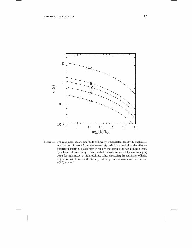
wherej1(x) = (sinx − x cosx)/x2. The term involvingj1 in the integrand is theFourier transform ofW (r). The functionσ(M) plays a crucial role in estimatesof the abundance of collapsed objects, and is plotted in Figure 3.1 as a function ofmass and redshift for the standard cosmological model. For modes with randomphases, the probability of different regions with the same size to have a perturba-tion amplitude betweenδ andδ + dδ is Gaussian with a zero mean and the abovevariance,P (δ)dδ = (2πσ2)−1/2 exp−δ2/2σ2dδ.
3.2 THE SMALLEST GAS CONDENSATIONS
As the density contrast between a spherical gas cloud and itscosmic environmentgrows, there are two main forces which come into play. The first is gravity and thesecond ispressure. We can get a rough estimate for the relative importance of theseforces from the following simple considerations. The increase in gas density nearthe center of the cloud sends out a pressure wave which propagates out at the speedof soundcs ∼ (kT/mp)
1/2 whereT is the gas temperature. The wave tries to evenout the density enhancement, consistent with the tendency of pressure to resist col-lapse. At the same time, gravity pulls the cloud together in the opposite direction.The characteristic time-scale for the collapse of the cloudis given by its radiusRdivided by the free-fall speed∼ (2GM/R)1/2, yieldingtcoll ∼ (G〈ρ〉)−1/2 where〈ρ〉 = M/ 4π
3 R3 is the characteristic density of the cloud as it turns aroundon itsway to collapse.iii If the sound wave does not have sufficient time to traverse the
iii Substituting the mean density of the Earth to this expression yields the characteristic time it takesa freely-falling elevator to reach the center of the Earth from its surface (∼ 1/3 of an hour), as well asthe order of magnitude of the time it takes a low-orbit satellite to go around the Earth (∼ 1.5 hours).
THE FIRST GAS CLOUDS 25
Figure 3.1 The root-mean-square amplitude of linearly-extrapolated density fluctuationsσas a function of massM (in solar massesM⊙, within a spherical top-hat filter) atdifferent redshiftsz. Halos form in regions that exceed the background densityby a factor of order unity. This threshold is only surpassed by rare (many-σ)peaks for high masses at high redshifts. When discussing theabundance of halosin §3.4, we will factor out the linear growth of perturbations and use the functionσ(M) at z = 0.
26 CHAPTER 3
cloud during the free-fall time, namelyR > RJ ≡ cstcoll, then the cloud willcollapse. Under these circumstances, the sound wave moves outward at a speedthat is slower than the inward motion of the gas, and so the wave is simply carriedalong together with the infalling material. On the other hand, the collapse will beinhibited by pressure for a sufficiently small cloud withR < RJ . The transitionbetween these regimes is defined by the so-called Jeans radius,RJ , correspondingto the Jeans mass,
MJ =4π
3〈ρ〉R3
J . (3.8)
This mass corresponds to the total gravitating mass of the cloud, including thedark matter. As long as the gas temperature is not very different from the CMBtemperature, the value ofMJ ∼ 105M⊙ is independent of redshift.6 This is theminimum total mass of the first gas cloud to collapse∼ 100 million years afterthe Big Bang. A few hundred million years later, once the cosmic gas was ionizedand heated to a temperatureT > 104K by the first galaxies, the minimum galaxymass had risen above∼ 108M⊙. At even later times, the UV light that filled upthe Universe was able to boil the uncooled gas out of the shallowest gravitationalpotential wells of mini-halos with a characteristic temperature below104K.7
As mentioned in§2, existing cosmological data suggests that the dark matteris“cold,” that is, its pressure is negligible during the gravitational growth of galaxies.In popular models, the Jeans mass of the dark matter alone is negligible but nonzero, of the order of the mass of a planet like Earth or Jupiter.8 All halos betweenthis minimum clump mass and∼ 105M⊙ are expected to contain mostly darkmatter and little ordinary matter.
3.3 SPHERICAL COLLAPSE AND HALO PROPERTIES
When an object above the Jeans mass collapses, the dark matter forms a halo insideof which the gas may cool, condense to the center, and eventually fragment intostars. The dark matter cannot cool since it has very weak interactions. As a result,a galaxy emerges with a central core that is occupied by starsand cold gas and issurrounded by an extended halo of invisible dark matter. Since cooling eliminatesthe pressure support from the gas, the only force that can prevent the gas fromsinking all the way to the center and ending up in a black hole is the centrifugalforce associated with its rotation around the center (angular momentum). The slight(∼ 5%) rotation, given to the gas by tidal torques from nearby galaxies as it turnsaround from the initial cosmic expansion and gets assembledinto the object, issufficient to stop its infall on a scale which isan order of magnitude smallerthan thesize of the dark matter halo9 (the so-called “virial radius”). On this stopping scale,the gas is assembled into a thin disk and orbits around the center for an extendedperiod of time, during which it tends to break into dense clouds which fragmentfurther into denser clumps. Within the compact clumps that are produced, the gasdensity is sufficiently high and the gas temperature is sufficiently low for the Jeansmass to be of order the mass of a star. As a result, the clumps fragment into starsand a galaxy is born.
THE FIRST GAS CLOUDS 27
In the popular cosmological model, small objects formed first. The very first starsmust have therefore formed inside gas condensations just above the cosmologicalJeans mass,∼ 105M⊙. Whereas each of these first gaseous halos was not massiveor cold enough to make more than a single high-mass star, starclusters started toform shortly afterwards inside bigger halos. By solving theequation of motion (2.1)for a spherical overdense region, it is possible to relate the characteristic radius andgravitational potential well of each of these galaxies to their mass and their redshiftof formation.
The small density fluctuations evidenced in the CMB grew overtime as describedin §3.1, until the perturbationsδ became of order unity and the full non-linear grav-itational collapse followed. The dynamical collapse of a dark matter halo can besolved analytically in spherical symmetry with an initial top-hat of uniform over-densityδi inside a sphere of radiusR. Although this toy model might seem artifi-cially simple, its results have turned out to be surprisingly accurate for interpretingthe properties and distribution of halos in numerical simulations of cold dark mat-ter.
During the gravitational collapse of a spherical region, the enclosed overdensityδ grows initially asδL = δiD(t)/D(ti), in accordance with linear theory, buteventuallyδ grows aboveδL. Any mass shell that is gravitationally bound (i.e.,with a negative total Newtonian energy) reaches a radius of maximum expansion(turn-around) and subsequently collapses. The solution ofthe equation of motionfor a top-hat region shows that at the moment when the region collapses to a point,the overdensity predicted by linear theory isδL = 1.686 in theΩm = 1 case, withonly a weak dependence onΩΛ in the more general case. Thus, a top-hat wouldhave collapsed at redshiftz if its linear overdensity extrapolated to the present day(also termed the critical density of collapse) is
δcrit(z) =1.686
D(z), (3.9)
where we setD(z = 0) = 1.Even a slight violation of the exact symmetry of the initial perturbation can pre-
vent the top-hat from collapsing to a point. Instead, the halo reaches a state of virialequilibrium through violent dynamical relaxation. We are familiar with the fact thatthe circular orbit of the Earth around the Sun has a kinetic energy which is half themagnitude of the gravitational potential energy. According to thevirial theorem,this happens to be a property shared by all dynamically relaxed, self-gravitatingsystems. We may therefore useU = −2K to relate the potential energyU to thekinetic energyK in the final state of a collapsed halo. This implies that the virialradius is half the turnaround radius (where the kinetic energy vanishes). Using thisresult, the final mean overdensity relative toρc at the collapse redshift turns out tobe∆c = 18π2 ≃ 178 in theΩm = 1 case,iv which applies at redshiftsz ≫ 1. Werestrict our attention below to these high redshifts.
ivThis implies that dynamical time within the virial radius ofgalaxies,∼ (Gρvir)−1/2, is of order
a tenth of the age of the Universe at any redshift.
28 CHAPTER 3
A halo of massM collapsing at redshiftz ≫ 1 thus has a virial radius
rvir = 1.5
(
M
108M⊙
)1/3 (
1 + z
10
)−1
kpc , (3.10)
and a corresponding circular velocity,
Vc =
(
GM
rvir
)1/2
= 17.0
(
M
108M⊙
)1/3 (
1 + z
10
)1/2
km s−1 . (3.11)
We may also define a virial temperature
Tvir =µmpV
2c
2k= 1.04 × 10⁴
( µ
0.6
)
(
M
108M⊙
)2/3 (
1 + z
10
)
K , (3.12)
whereµ is the mean molecular weight andmp is the proton mass. Note that thevalue ofµ depends on the ionization fraction of the gas; for a fully ionized pri-mordial gasµ = 0.59, while a gas with ionized hydrogen but only singly-ionizedhelium hasµ = 0.61. The binding energy of the halo is approximately,
Eb =1
2
GM2
rvir= 2.9 × 1053
(
M
108M⊙
)5/3 (
1 + z
10
)
erg . (3.13)
Note that if the ordinary matter traces the dark matter, its total binding energy issmaller thanEb by a factor ofΩb/Ωm, and could be lower than the energy outputof a single supernovav (∼ 1051 ergs) for the first generation of dwarf galaxies.
Although spherical collapse captures some of the physics governing the forma-tion of halos, structure formation in cold dark matter models proceeds hierarchi-cally. At early times, most of the dark matter was in low-masshalos, and thesehalos then continuously accreted and merged to form high-mass halos. Numericalsimulations of hierarchical halo formation indicate a roughly universal spherically-averaged density profile for the resulting halos, though with considerable scatteramong different halos. This profile has the formvi
ρ(r) =3H2
0
8πG(1 + z)3Ωm
δc
cNx(1 + cNx)2, (3.14)
wherex = r/rvir, and the characteristic densityδc is related to the concentrationparametercN by
δc =∆c
3
c3N
ln(1 + cN) − cN/(1 + cN). (3.15)
The concentration parameter itself depends on the halo massM , at a given redshiftz, with a value of order∼ 4 for newly collapsed halos.
vA supernova is the explosion that follows the death of a massive star.viThis functional form is commonly labeled as the ‘NFW profile’after the original paper by Navarro,
J. F., Frenk, C. S. & White, S. D. M.Astrophys. J.490, 493 (1997).
THE FIRST GAS CLOUDS 29
3.4 ABUNDANCE OF DARK MATTER HALOS
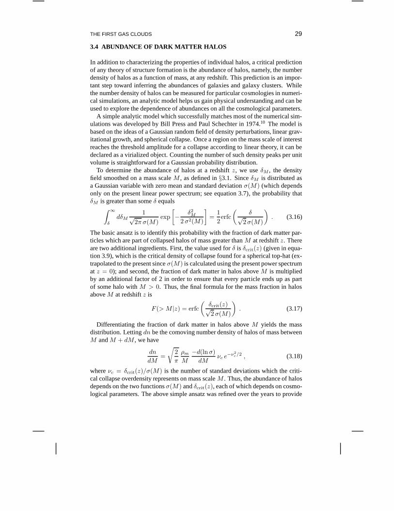
In addition to characterizing the properties of individualhalos, a critical predictionof any theory of structure formation is the abundance of halos, namely, the numberdensity of halos as a function of mass, at any redshift. This prediction is an impor-tant step toward inferring the abundances of galaxies and galaxy clusters. Whilethe number density of halos can be measured for particular cosmologies in numeri-cal simulations, an analytic model helps us gain physical understanding and can beused to explore the dependence of abundances on all the cosmological parameters.
A simple analytic model which successfully matches most of the numerical sim-ulations was developed by Bill Press and Paul Schechter in 1974.10 The model isbased on the ideas of a Gaussian random field of density perturbations, linear grav-itational growth, and spherical collapse. Once a region on the mass scale of interestreaches the threshold amplitude for a collapse according tolinear theory, it can bedeclared as a virialized object. Counting the number of suchdensity peaks per unitvolume is straightforward for a Gaussian probability distribution.
To determine the abundance of halos at a redshiftz, we useδM , the densityfield smoothed on a mass scaleM , as defined in§3.1. SinceδM is distributed asa Gaussian variable with zero mean and standard deviationσ(M) (which dependsonly on the present linear power spectrum; see equation 3.7), the probability thatδM is greater than someδ equals
∫ ∞
δ
dδM1√
2π σ(M)exp
[
− δ2M
2 σ2(M)
]
=1
2erfc
(
δ√2σ(M)
)
. (3.16)
The basic ansatz is to identify this probability with the fraction of dark matter par-ticles which are part of collapsed halos of mass greater thanM at redshiftz. Thereare two additional ingredients. First, the value used forδ is δcrit(z) (given in equa-tion 3.9), which is the critical density of collapse found for a spherical top-hat (ex-trapolated to the present sinceσ(M) is calculated using the present power spectrumat z = 0); and second, the fraction of dark matter in halos aboveM is multipliedby an additional factor of 2 in order to ensure that every particle ends up as partof some halo withM > 0. Thus, the final formula for the mass fraction in halosaboveM at redshiftz is
F (> M |z) = erfc
(
δcrit(z)√2 σ(M)
)
. (3.17)
Differentiating the fraction of dark matter in halos aboveM yields the massdistribution. Lettingdn be the comoving number density of halos of mass betweenM andM + dM , we have
dn
dM=
√
2
π
ρm
M
−d(lnσ)
dMνc e−ν2
c/2 , (3.18)
whereνc = δcrit(z)/σ(M) is the number of standard deviations which the criti-cal collapse overdensity represents on mass scaleM . Thus, the abundance of halosdepends on the two functionsσ(M) andδcrit(z), each of which depends on cosmo-logical parameters. The above simple ansatz was refined overthe years to provide
30 CHAPTER 3
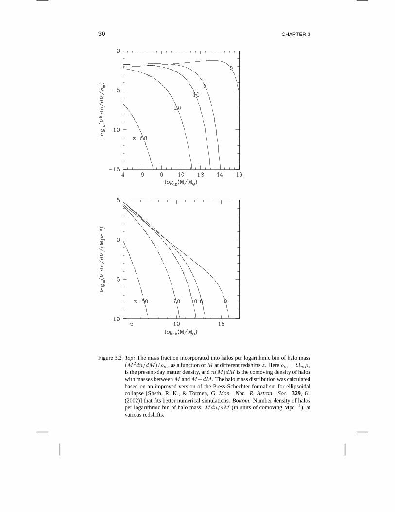
Figure 3.2 Top: The mass fraction incorporated into halos per logarithmic bin of halo mass(M2dn/dM)/ρm, as a function ofM at different redshiftsz. Hereρm = Ωmρc
is the present-day matter density, andn(M)dM is the comoving density of haloswith masses betweenM andM+dM . The halo mass distribution was calculatedbased on an improved version of the Press-Schechter formalism for ellipsoidalcollapse [Sheth, R. K., & Tormen, G.Mon. Not. R. Astron. Soc.329, 61(2002)] that fits better numerical simulations.Bottom:Number density of halosper logarithmic bin of halo mass,Mdn/dM (in units of comoving Mpc−3), atvarious redshifts.
THE FIRST GAS CLOUDS 31
a better match to numerical simulation. Results for the comoving density of halosof different masses at different redshifts are shown in Figure 3.2.
The ad-hoc factor of 2 in the Press-Schechter derivation is necessary, since other-wise only positive fluctuations ofδM would be included. Bond et al. (1991) foundan alternate derivation of this correction factor, using a different ansatz, called theexcursion set (or extended Press-Schechter) formalism.11 In their derivation, thefactor of 2 has a more satisfactory origin. For a given massM , even if δM issmaller thanδcrit(z), it is possible that the corresponding region lies inside a re-gion of some larger massML > M , with δML
> δcrit(z). In this case the originalregion should be counted as belonging to a halo of massML. Thus, the fractionof particles which are part of collapsed halos of mass greater thanM is larger thanthe expression given in equation (3.16).
The Press-Schechter formalism makes no attempt to deal withthe correlationsamong halos or between different mass scales. This means that while it can gen-erate a distribution of halos at two different epochs, it says nothing about howparticular halos in one epoch are related to those in the second. We therefore wouldlike some method to predict, at least statistically, the growth of individual halosvia accretion and mergers. Even restricting ourselves to spherical collapse, such amodel must utilize the full spherically-averaged density profile around a particularpoint. The potential correlations between the mean overdensities at different radiimake the statistical description substantially more difficult.
The excursion set formalism seeks to describe the statistics of halos by consider-ing the statistical properties ofδ(R), the average overdensity within some sphericalwindow of characteristic radiusR, as a function ofR. While the Press-Schechtermodel depends only on the Gaussian distribution ofδ for one particularR, the ex-cursion set considers allR. Again the connection between a value of the linearregimeδ and the final state is made via the spherical collapse solution so that thereis a critical valueδcrit(z) of δ which is required for collapse at a redshiftz.
For most choices of window function, the functionsδ(R) are correlated from oneR to another such that it is prohibitively difficult to calculate the desired statisticsdirectly. However, for one particular choice of a window function, the correlationsbetween differentR greatly simplify and many interesting quantities may be cal-culated.12 The key is to use ak-space top-hat window function, namely,Wk = 1for all k less than some criticalkc andWk = 0 for k > kc. This filter has a spa-tial form of W (r) ∝ j1(kcr)/kcr, which implies a comoving volume6π2/k3
c ormass6π2ρm/k3
c . The characteristic radius of the filter is∼ k−1c , as expected. Note
that in real space, this window function exhibits a sinusoidal oscillation and is notsharply localized.
The great advantage of the sharpk-space filter is that the difference at a givenpoint betweenδ on one mass scale and that on another mass scale is statisticallyindependent from the value on the larger mass scale. With a Gaussian random field,eachδk is Gaussian distributed independently from the others. Forthis filter,
δ(M) =
∫
k<kc(M)
d3k
(2π)3δk, (3.19)
meaning that the overdensity on a particular scale is simplythe sum of the random
32 CHAPTER 3
variablesδk interior to the chosenkc. Consequently, the difference between theδ(M) on two mass scales is just the sum of theδk in the sphericalk-shell betweenthe twokc, which is independent from the sum of theδk interior to the smallerkc.Meanwhile, the distribution ofδ(M) given no prior information is still a Gaussianof mean zero and variance
σ2(M) =1
2π2
∫
k<kc(M)
dk k2P (k). (3.20)
If we now considerδ as a function of scalekc, we see that we begin fromδ = 0at kc = 0 (M = ∞) and then add independently random pieces askc increases.This generates a random walk, albeit one whose stepsize varies withkc. We thenassume that at redshiftz, a given functionδ(kc) represents a collapsed massMcorresponding to thekc where the function first crosses the critical valueδcrit(z).With this assumption, we may use the properties of random walks to calculate theevolution of the mass as a function of redshift.
It is now easy to re-derive the Press-Schechter mass function, including the pre-viously unexplained factor of 2. The fraction of mass elements included in halos ofmass less thanM is just the probability that a random walk remains belowδcrit(z)for all kc less thanKc, the filter cutoff appropriate toM . This probability mustbe the complement of the sum of the probabilities that(a) δ(Kc) > δcrit(z), orthat (b) δ(Kc) < δcrit(z) but δ(k′
c) > δcrit(z) for somek′c < Kc. But these
two cases in fact have equal probability; any random walk belonging to class(a) may be reflected around its first upcrossing ofδcrit(z) to produce a walk ofclass (b), and vice versa. Since the distribution ofδ(Kc) is simply Gaussianwith varianceσ2(M), the fraction of random walks falling into class(a) is simply(1/
√2πσ2)
∫ ∞δcrit(z) dδ exp−δ2/2σ2(M). Hence, the fraction of mass elements
included in halos of mass less thanM at redshiftz is simply
F (< M) = 1 − 2 × 1√2πσ2
∫ ∞
δcrit(z)
dδ exp
− δ2
2σ2(M)
, (3.21)
which may be differentiated to yield the Press-Schechter mass function. We maynow go further and consider how halos at one redshift are related to those at anotherredshift. If it is given that a halo of massM2 exists at redshiftz2, then we knowthat the random functionδ(kc) for each mass element within the halo first crossesδ(z2) at kc2 corresponding toM2. Given this constraint, we may study the distri-bution of kc where the functionδ(kc) crosses other thresholds. It is particularlyeasy to construct the probability distribution for when trajectories first cross someδcrit(z1) > δcrit(z2) (implying z1 > z2); clearly this occurs at somekc1 > kc2.This problem reduces to the previous one if we translate the origin of the randomwalks from(kc, δ) = (0, 0) to (kc2, δcrit(z2)). We therefore find the distributionof halo massesM1 that a mass element finds itself in at redshiftz1, given that it ispart of a larger halo of massM2 at a later redshiftz2, is
dP
dM1(M1, z1|M2, z2) =
√
2
π
δcrit(z1) − δcrit(z2)
[σ2(M1) − σ2(M2)]3/2
∣
∣
∣
∣
dσ(M1)
dM1
∣
∣
∣
∣
exp
− [δcrit(z1) − δcrit(z2)]2
2[σ2(M1) − σ2(M2)]
.
(3.22)
THE FIRST GAS CLOUDS 33
This may be rewritten as saying that the quantity
v =δcrit(z1) − δcrit(z2)
√
σ2(M1) − σ2(M2)(3.23)
is distributed as the positive half of a Gaussian with unit variance; equation (3.23)may be inverted to findM1(v).
We can interpret the statistics of these random walks as those of merging and ac-creting halos. For a single halo, we may imagine that as we look back in time, theobject breaks into ever smaller pieces, similar to the branching of a tree. Equation(3.22) is the distribution of the sizes of these branches at some given earlier time.However, using this description of the ensemble distribution to generate randomrealizations of single merger trees has proven to be difficult. In all cases, one re-cursively steps back in time, at each step breaking the final object into two or morepieces. A simplified scheme may assume that at each time step,the object breaksinto only two pieces. One value from the distribution (3.22)then determines themass ratio of the two branches.
We may also use the distribution of the ensemble to derive some additional an-alytic results. A useful example is the distribution of the epoch at which an objectthat has massM2 at redshiftz2 has accumulated half of its mass. The probabilitythat the formation time is earlier thanz1 can be defined as the probability that atredshiftz1 a progenitor whose mass exceedsM2/2 exists:
P (zf > z1) =
∫ M2
M2/2
M2
M
dP
dM(M, z1|M2, z2)dM, (3.24)
wheredP/dM is given in equation (3.22). The factor ofM2/M corrects the count-ing from being mass weighted to number weighted; each halo ofmassM2 can haveonly one progenitor of mass greater thanM2/2. Differentiating equation (3.24)with respect to time gives the distribution of formation times. Overall, the excursionset formalism provides a good approximation to more exact numerical simulationsof halo assembly and merging histories.
3.5 COOLING AND CHEMISTRY
When a dark matter halo collapses, the associated gas falls in at a speed of orderVc in equation (3.11). When multiple gas streams collide and settle to a staticconfiguration, the gas shocks to the virial temperatureTvir in equation (3.12), atwhich it is held against gravity by its thermal pressure. In order for fragmentationto occur and stars to form, the collapsed gas has to cool and get denser until itsJeans mass drops to the mass scale of individual stars.
Cooling of the gas in the Milky Way galaxy (the so-called “interstellar medium”)is controlled by abundant heavy elements, such as carbon, oxygen, or nitrogen,which were produced in the interiors of stars. However, before the first stars formedthere were no such heavy elements around and the gas was able to cool only throughradiative transitions of atomic and molecular hydrogen. Figure 3.3 illustrates the
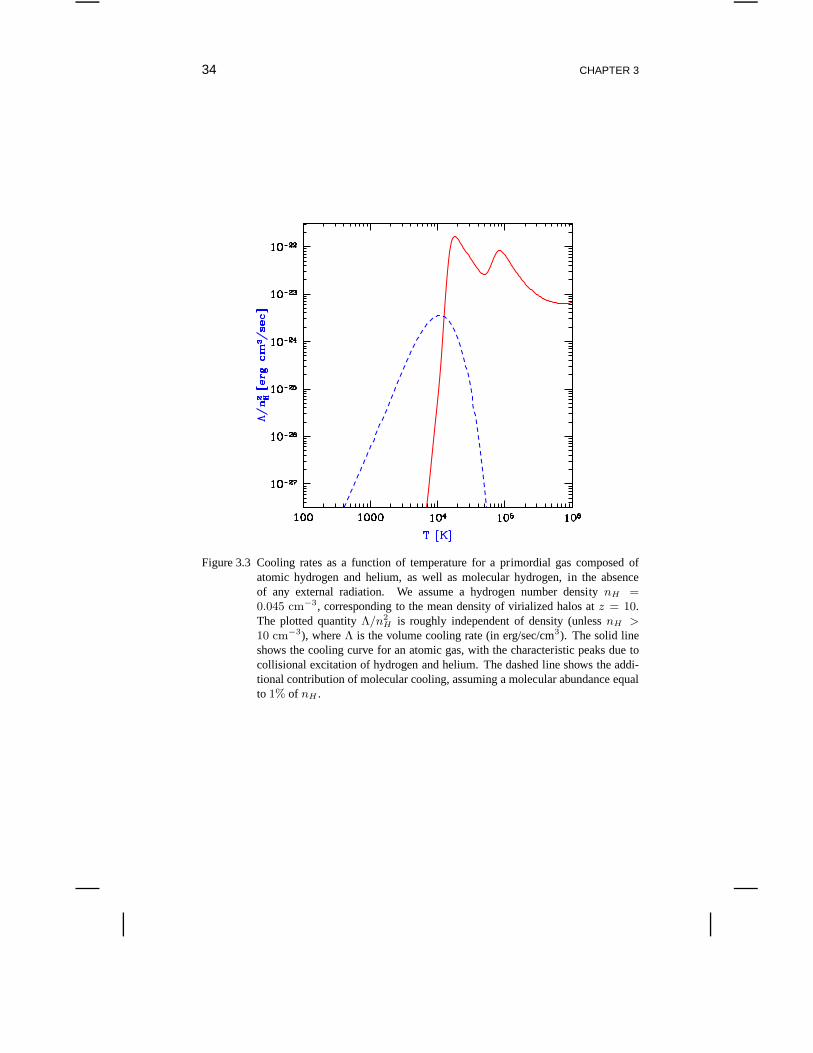
34 CHAPTER 3
Figure 3.3 Cooling rates as a function of temperature for a primordial gas composed ofatomic hydrogen and helium, as well as molecular hydrogen, in the absenceof any external radiation. We assume a hydrogen number density nH =0.045 cm−3, corresponding to the mean density of virialized halos atz = 10.The plotted quantityΛ/n2
H is roughly independent of density (unlessnH >10 cm−3), whereΛ is the volume cooling rate (in erg/sec/cm3). The solid lineshows the cooling curve for an atomic gas, with the characteristic peaks due tocollisional excitation of hydrogen and helium. The dashed line shows the addi-tional contribution of molecular cooling, assuming a molecular abundance equalto 1% of nH .
THE FIRST GAS CLOUDS 35
cooling rate of the primordial gas as a function of its temperature. Below a temper-ature of∼ 104K, atomic transitions are not effective because collisionsamong theatoms do not carry sufficient energy to excite the atoms and cause them to emit ra-diation through the decay of the excited states. Since the first gas clouds around theJeans mass had a virial temperature well below104K, cooling and fragmentationof the gas had to rely on an alternative coolant with sufficiently low energy levelsand a correspondingly low excitation temperature, namely molecular hydrogen, H2.Hydrogen molecules could have formed through a rare chemical reaction involvingthe negative hydrogen (H−) ion: H+e− →H−+photon, and H−+H→H2+e−, inwhich free electrons (e−) act as catalysts. After cosmological recombination, theH2 abundance was negligible. However, inside the first gas clouds, there was asufficient abundance of free electrons to catalyze H2 and cool the gas to tempera-tures as low as hundreds of degrees K (similar to the temperature range presentlyon Earth).
However, the hydrogen molecule is fragile and can easily be broken by UV pho-tons (with energies in the range of 11.26-13.6 eV),vii to which the cosmic gas istransparent even before it is ionized.13 The first population of stars was thereforesuicidal. As soon as the very early stars formed and produceda background ofUV light, this background light dissociated molecular hydrogen and suppressedthe prospects for the formation of similar stars inside distant halos with low virialtemperaturesTvir.
As soon as halos withTvir > 104K formed, atomic hydrogen was able to cool thegas in them and allow fragmentation even in the absence of H2. In addition, oncethe gas was enriched with heavy elements, it was able to cool even more efficiently.
3.6 SHEETS, FILAMENTS, AND ONLY THEN, GALAXIES
The development of large scale cosmic structures occurs in three stages, as orig-inally recognized by the Soviet physicist Yakov Zel’dovich. First, a region col-lapses along one axis, making a two-dimensional sheet. Thenthe sheet collapsesalong the second axis, making a one-dimensional filament. Finally, the filamentcollapses along the third axis into a virialized halo. A snapshot of the distributionof dark matter at a given cosmic time should show a mix of thesegeometries indifferent regions that reached different evolutionary stages (owing to their differ-ent densities). The sheets define the boundary of voids from where their materialwas assembled; the intersection of sheets define filaments, and the intersection offilaments define halos – into which the material is ultimatelydrained. The result-ing network of structures, shown in Figure 3.4, delineates the so-called “cosmicweb.” Gas tends to follow the dark matter except within shallow potential wellsinto which it does not assemble, owing to its finite pressure.Computer simula-tions have provided highly accurate maps of how the dark matter is expected tobe distributed since its dynamics is dictated only by gravity, but unfortunately, thismatter is invisible. As soon as ordinary matter is added, complexity arises because
vii 1 electron Volt (eV) is an energy unit equivalent to1.6 × 10−12ergs or 11,604K.
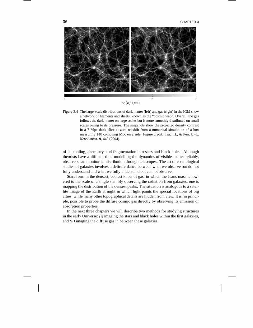
36 CHAPTER 3
Figure 3.4 The large-scale distributions of dark matter (left) and gas (right) in the IGM showa network of filaments and sheets, known as the “cosmic web”. Overall, the gasfollows the dark matter on large scales but is more smoothly distributed on smallscales owing to its pressure. The snapshots show the projected density contrastin a 7 Mpc thick slice at zero redshift from a numerical simulation of a boxmeasuring140 comoving Mpc on a side. Figure credit: Trac, H., & Pen, U.-L.New Astron.9, 443 (2004).
of its cooling, chemistry, and fragmentation into stars andblack holes. Althoughtheorists have a difficult time modelling the dynamics of visible matter reliably,observers can monitor its distribution through telescopes. The art of cosmologicalstudies of galaxies involves a delicate dance between what we observe but do notfully understand and what we fully understand but cannot observe.
Stars form in the densest, coolest knots of gas, in which the Jeans mass is low-ered to the scale of a single star. By observing the radiationfrom galaxies, one ismapping the distribution of the densest peaks. The situation is analogous to a satel-lite image of the Earth at night in which light paints the special locations of bigcities, while many other topographical details are hidden from view. It is, in princi-ple, possible to probe the diffuse cosmic gas directly by observing its emission orabsorption properties.
In the next three chapters we will describe two methods for studying structuresin the early Universe:(i) imaging the stars and black holes within the first galaxies,and(ii) imaging the diffuse gas in between these galaxies.
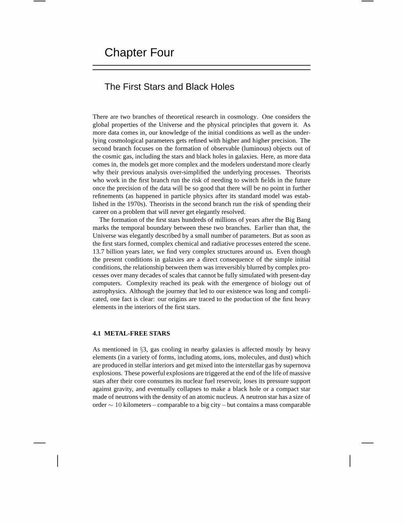
Chapter Four
The First Stars and Black Holes
There are two branches of theoretical research in cosmology. One considers theglobal properties of the Universe and the physical principles that govern it. Asmore data comes in, our knowledge of the initial conditions as well as the under-lying cosmological parameters gets refined with higher and higher precision. Thesecond branch focuses on the formation of observable (luminous) objects out ofthe cosmic gas, including the stars and black holes in galaxies. Here, as more datacomes in, the models get more complex and the modelers understand more clearlywhy their previous analysis over-simplified the underlyingprocesses. Theoristswho work in the first branch run the risk of needing to switch fields in the futureonce the precision of the data will be so good that there will be no point in furtherrefinements (as happened in particle physics after its standard model was estab-lished in the 1970s). Theorists in the second branch run the risk of spending theircareer on a problem that will never get elegantly resolved.
The formation of the first stars hundreds of millions of yearsafter the Big Bangmarks the temporal boundary between these two branches. Earlier than that, theUniverse was elegantly described by a small number of parameters. But as soon asthe first stars formed, complex chemical and radiative processes entered the scene.13.7 billion years later, we find very complex structures around us. Even thoughthe present conditions in galaxies are a direct consequenceof the simple initialconditions, the relationship between them was irreversibly blurred by complex pro-cesses over many decades of scales that cannot be fully simulated with present-daycomputers. Complexity reached its peak with the emergence of biology out ofastrophysics. Although the journey that led to our existence was long and compli-cated, one fact is clear: our origins are traced to the production of the first heavyelements in the interiors of the first stars.
4.1 METAL-FREE STARS
As mentioned in§3, gas cooling in nearby galaxies is affected mostly by heavyelements (in a variety of forms, including atoms, ions, molecules, and dust) whichare produced in stellar interiors and get mixed into the interstellar gas by supernovaexplosions. These powerful explosions are triggered at theend of the life of massivestars after their core consumes its nuclear fuel reservoir,loses its pressure supportagainst gravity, and eventually collapses to make a black hole or a compact starmade of neutrons with the density of an atomic nucleus. A neutron star has a size oforder∼ 10 kilometers – comparable to a big city – but contains a mass comparable
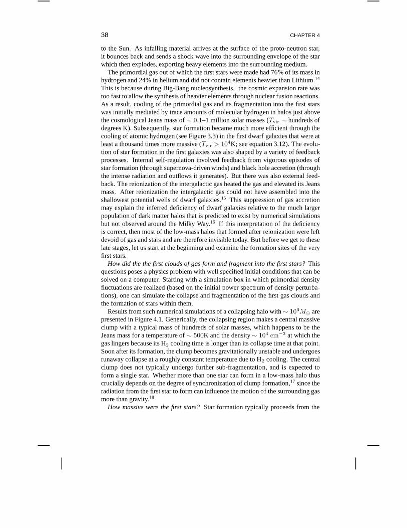
38 CHAPTER 4
to the Sun. As infalling material arrives at the surface of the proto-neutron star,it bounces back and sends a shock wave into the surrounding envelope of the starwhich then explodes, exporting heavy elements into the surrounding medium.
The primordial gas out of which the first stars were made had 76% of its mass inhydrogen and 24% in helium and did not contain elements heavier than Lithium.14
This is because during Big-Bang nucleosynthesis, the cosmic expansion rate wastoo fast to allow the synthesis of heavier elements through nuclear fusion reactions.As a result, cooling of the primordial gas and its fragmentation into the first starswas initially mediated by trace amounts of molecular hydrogen in halos just abovethe cosmological Jeans mass of∼ 0.1–1 million solar masses (Tvir ∼ hundreds ofdegrees K). Subsequently, star formation became much more efficient through thecooling of atomic hydrogen (see Figure 3.3) in the first dwarfgalaxies that were atleast a thousand times more massive (Tvir > 104K; see equation 3.12). The evolu-tion of star formation in the first galaxies was also shaped bya variety of feedbackprocesses. Internal self-regulation involved feedback from vigorous episodes ofstar formation (through supernova-driven winds) and blackhole accretion (throughthe intense radiation and outflows it generates). But there was also external feed-back. The reionization of the intergalactic gas heated the gas and elevated its Jeansmass. After reionization the intergalactic gas could not have assembled into theshallowest potential wells of dwarf galaxies.15 This suppression of gas accretionmay explain the inferred deficiency of dwarf galaxies relative to the much largerpopulation of dark matter halos that is predicted to exist bynumerical simulationsbut not observed around the Milky Way.16 If this interpretation of the deficiencyis correct, then most of the low-mass halos that formed afterreionization were leftdevoid of gas and stars and are therefore invisible today. But before we get to theselate stages, let us start at the beginning and examine the formation sites of the veryfirst stars.
How did the the first clouds of gas form and fragment into the first stars?Thisquestions poses a physics problem with well specified initial conditions that can besolved on a computer. Starting with a simulation box in whichprimordial densityfluctuations are realized (based on the initial power spectrum of density perturba-tions), one can simulate the collapse and fragmentation of the first gas clouds andthe formation of stars within them.
Results from such numerical simulations of a collapsing halo with∼ 106M⊙ arepresented in Figure 4.1. Generically, the collapsing region makes a central massiveclump with a typical mass of hundreds of solar masses, which happens to be theJeans mass for a temperature of∼ 500K and the density∼ 104 cm−3 at which thegas lingers because its H2 cooling time is longer than its collapse time at that point.Soon after its formation, the clump becomes gravitationally unstable and undergoesrunaway collapse at a roughly constant temperature due to H2 cooling. The centralclump does not typically undergo further sub-fragmentation, and is expected toform a single star. Whether more than one star can form in a low-mass halo thuscrucially depends on the degree of synchronization of clumpformation,17 since theradiation from the first star to form can influence the motion of the surrounding gasmore than gravity.18
How massive were the first stars?Star formation typically proceeds from the
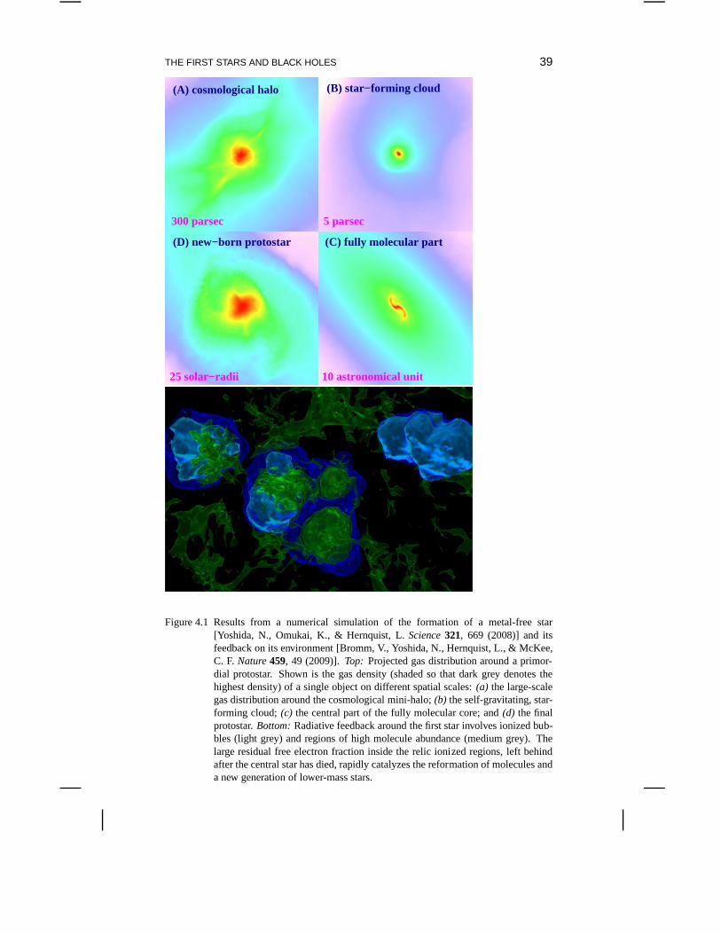
THE FIRST STARS AND BLACK HOLES 39
300 parsec 5 parsec
10 astronomical unit25 solar−radii
(A) cosmological halo (B) star−forming cloud
(C) fully molecular part(D) new−born protostar
Figure 4.1 Results from a numerical simulation of the formation of a metal-free star[Yoshida, N., Omukai, K., & Hernquist, L.Science321, 669 (2008)] and itsfeedback on its environment [Bromm, V., Yoshida, N., Hernquist, L., & McKee,C. F.Nature459, 49 (2009)]. Top: Projected gas distribution around a primor-dial protostar. Shown is the gas density (shaded so that darkgrey denotes thehighest density) of a single object on different spatial scales: (a) the large-scalegas distribution around the cosmological mini-halo;(b) the self-gravitating, star-forming cloud;(c) the central part of the fully molecular core; and(d) the finalprotostar.Bottom:Radiative feedback around the first star involves ionized bub-bles (light grey) and regions of high molecule abundance (medium grey). Thelarge residual free electron fraction inside the relic ionized regions, left behindafter the central star has died, rapidly catalyzes the reformation of molecules anda new generation of lower-mass stars.
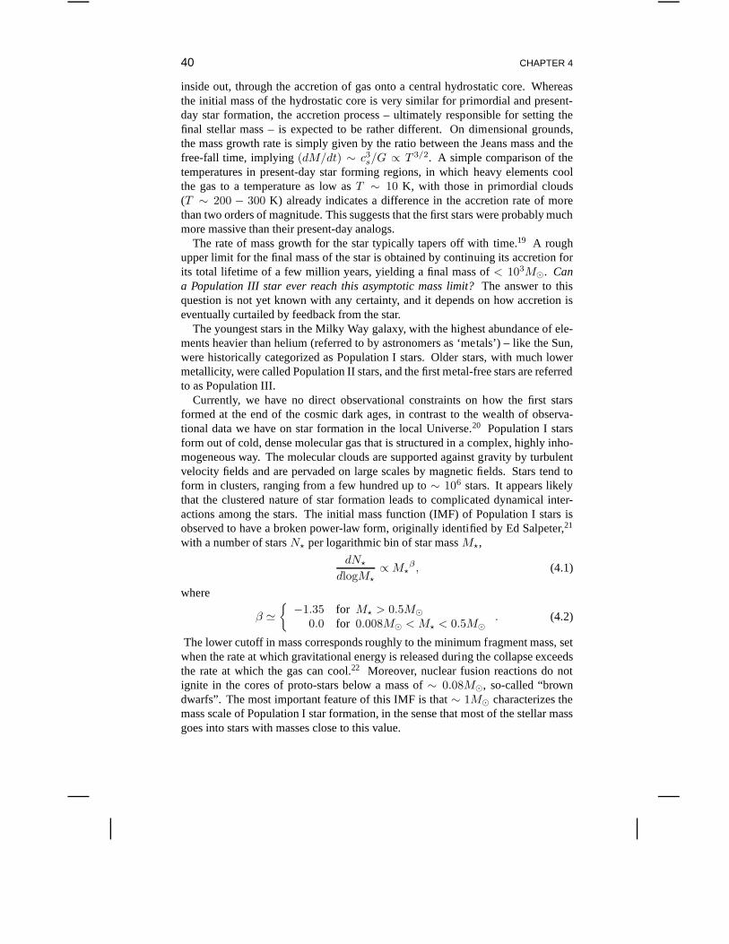
40 CHAPTER 4
inside out, through the accretion of gas onto a central hydrostatic core. Whereasthe initial mass of the hydrostatic core is very similar for primordial and present-day star formation, the accretion process – ultimately responsible for setting thefinal stellar mass – is expected to be rather different. On dimensional grounds,the mass growth rate is simply given by the ratio between the Jeans mass and thefree-fall time, implying(dM/dt) ∼ c3
s/G ∝ T 3/2. A simple comparison of thetemperatures in present-day star forming regions, in whichheavy elements coolthe gas to a temperature as low asT ∼ 10 K, with those in primordial clouds(T ∼ 200 − 300 K) already indicates a difference in the accretion rate of morethan two orders of magnitude. This suggests that the first stars were probably muchmore massive than their present-day analogs.
The rate of mass growth for the star typically tapers off withtime.19 A roughupper limit for the final mass of the star is obtained by continuing its accretion forits total lifetime of a few million years, yielding a final mass of < 103M⊙. Cana Population III star ever reach this asymptotic mass limit?The answer to thisquestion is not yet known with any certainty, and it depends on how accretion iseventually curtailed by feedback from the star.
The youngest stars in the Milky Way galaxy, with the highest abundance of ele-ments heavier than helium (referred to by astronomers as ‘metals’) – like the Sun,were historically categorized as Population I stars. Olderstars, with much lowermetallicity, were called Population II stars, and the first metal-free stars are referredto as Population III.
Currently, we have no direct observational constraints on how the first starsformed at the end of the cosmic dark ages, in contrast to the wealth of observa-tional data we have on star formation in the local Universe.20 Population I starsform out of cold, dense molecular gas that is structured in a complex, highly inho-mogeneous way. The molecular clouds are supported against gravity by turbulentvelocity fields and are pervaded on large scales by magnetic fields. Stars tend toform in clusters, ranging from a few hundred up to∼ 106 stars. It appears likelythat the clustered nature of star formation leads to complicated dynamical inter-actions among the stars. The initial mass function (IMF) of Population I stars isobserved to have a broken power-law form, originally identified by Ed Salpeter,21
with a number of starsN⋆ per logarithmic bin of star massM⋆,
dN⋆
dlogM⋆∝ M⋆
β , (4.1)
where
β ≃
−1.35 for M⋆ > 0.5M⊙0.0 for 0.008M⊙ < M⋆ < 0.5M⊙
. (4.2)
The lower cutoff in mass corresponds roughly to the minimum fragment mass, setwhen the rate at which gravitational energy is released during the collapse exceedsthe rate at which the gas can cool.22 Moreover, nuclear fusion reactions do notignite in the cores of proto-stars below a mass of∼ 0.08M⊙, so-called “browndwarfs”. The most important feature of this IMF is that∼ 1M⊙ characterizes themass scale of Population I star formation, in the sense that most of the stellar massgoes into stars with masses close to this value.
THE FIRST STARS AND BLACK HOLES 41
Since current simulations indicate that the first stars werepredominantly verymassive (> 30M⊙), and consequently rather different from present-day stellar pop-ulations, an interesting question arises:how and when did the transition take placefrom the early formation of massive stars to the late-time formation of low-massstars?
The very first stars formed under conditions that were much simpler than thehighly complex birth places of stars in present-day molecular clouds. As soonas these stars appeared, however, the situation became morecomplex due to theirfeedback on the environment. In particular, supernova explosions dispersed theheavy elements produced inside the first generation of starsinto the surroundinggas. Atomic and molecular cooling became much more efficientafter the additionof these metals.
Early metal enrichment was likely the dominant effect that brought about thetransition from Population III to Population II star formation. Simple consider-ations indicate that as soon as the heavy element abundance exceeded a level assmall as 0.1% (or even lower) of the solar abundance, the cooling of the gas becamemuch more efficient than that provided by H2 molecules.23 The characteristic massscale for star formation is therefore expected to be a function of metallicity, witha sharp transition at this metallicity threshold, above which the characteristic massof a star gets reduced by about two orders of magnitude. Nevertheless, one shouldkeep in mind that the temperature floor of the gas was dictatedby the CMB (whosetemperature was54.6 × [(1 + z)/20] K) and therefore even with efficient cooling,the stars at high redshifts were likely more massive than thestars found today.
The maximum distance out to which a galactic outflow mixes heavy elementswith the IGM can be estimated based on energy considerations. The mechanical en-ergy releasedE will accelerate all the gas it encounters into a thin shell ata physicaldistanceRmax from the central source. In doing so, it must accelerate the swept-upgas to the Hubble flow velocity at that distance,vs = H(z)Rmax. If the shocked gashas a short cooling time, then its original kinetic energy islost and is unavailable forexpanding the shell. Ignoring the gravitational effect of the host galaxy, deviationsfrom the Hubble flow, and cooling inside the cavity bounded bythe shell, energyconservation implies:E = 1
2Msv2s , whereMs = 4π
3 ρR3max. At z ≫ 1, this gives
a maximum outflow distance:Rmax ∼ 50 kpc(E/1056 ergs)1/5[(1 + z)/10]−6/5.The maximum radius of influence from a galactic outflow can therefore be es-timated based on the total number of supernovae that power it(each releasing∼ 1051 ergs of which a substantial fraction may be lost by early cooling)or themassMbh of the central black hole (typically releasing a fraction ofa percent ofMbhc
2 in mechanical energy). More detailed calculations give similar results.24
Finally, the fraction of the IGM enriched with heavy elements can be obtained bymultiplying the density of galactic halos with their individual volumes of influence.
Since the earliest galaxies represent high density peaks and are therefore clus-tered, the metal enrichment process was inherently non-uniform. The early evolu-tion of the volume filling of metals in the IGM can be inferred from the spectra ofbright high-redshift sources.25 Even at late cosmic times, it should be possible tofind regions of the Universe that are composed of primordial gas and hence could
42 CHAPTER 4
make Population III stars. Since massive stars produce ionizing photons much moreeffectively than low-mass stars, the transition from Population III to Population IIstars had important consequences for the ionization history of the cosmic gas. By aredshift ofz ∼ 5, the average metal abundance in the IGM is observed to be∼ 1%of the solar value, as expected from the heavy element yield of the same massivestars that reionized the Universe.26
4.2 PROPERTIES OF THE FIRST STARS
Primordial stars that are hundreds of times more massive than the Sun have an effec-tive surface temperatureTeff approaching∼ 105 K, with only a weak dependenceon their mass. This temperature is∼ 17 times higher than the surface temperatureof the Sun,∼ 5800 K. These massive stars are held against their self-gravity by ra-diation pressure, having the so-calledEddington luminosity(see derivation in§4.3)which is strictly proportional to their massM⋆,
LE = 1.3 × 1040
(
M⋆
100M⊙
)
erg s−1, (4.3)
and is a few million times more luminous than the Sun,L⊙ = 4 × 1033 erg s−1.Because of these characteristics, the total luminosity andcolor of a cluster of suchstars simply depends on its total mass and not on the mass distribution of starswithin it. The radii of these starsR⋆ can be calculated by equating their luminosityto the emergent blackbody fluxσT 4
eff times their surface area4πR2⋆ (whereσ =
5.67 × 10⁻⁵ erg cm−2 s−1 deg−4 is the Stefan-Boltzmann constant). This gives
R⋆ =
(
LE
4πσT 4eff
)1/2
= 4.3 × 1011 cm ×(
M⋆
100M⊙
)1/2
, (4.4)
which is∼ 6 times larger than the radius of the Sun,R⊙ = 7 × 1010 cm.The high surface temperature of the first stars makes them ideal factories of ion-
izing photons. To free (ionize) an electron out of a hydrogenatom requires anenergy of 13.6eV (equivalent, through a division by Boltzmann’s constantkB , to atemperature of∼ 1.6 × 10⁵K), which is coincidentally the characteristic energy ofa photon emitted by the first massive stars.
The first stars had lifetimes of a few million years, independent of their mass.During its lifetime, a Population III star produced∼ 105 ionizing photons perproton incorporated in it. This means that only a tiny fraction (> 10−5) of all thehydrogen in the Universe needs to be assembled into Population III stars in orderfor there to be sufficient photons to ionize the rest of the cosmic gas. The actualrequired star formation efficiency depends on the fraction of all ionizing photonsthat escape from the host galaxies into the intergalactic space (fesc) rather thenbeing absorbed by hydrogen inside these galaxies.27 For comparison, PopulationII stars produce on average∼ 4, 000 ionizing photons per proton in them. If theUniverse was ionized by such stars, then a much larger fraction (by a factor of∼ 25) of its gaseous content had to be converted into stars in order to have thesame effect as Population III stars.
THE FIRST STARS AND BLACK HOLES 43
The first stars had a large impact on their gaseous environment. Their UV emis-sion ionized and heated the surrounding gas, and their windsor supernova explo-sions pushed the gas around like a piston. Such feedback effects controlled theoverall star formation efficiency within each galaxy,f⋆. This efficiency is likelyto have been small in the earlier galaxies that had shallow potential wells, and it ispossible that the subsequent Population II stars dominatedthe production of ioniz-ing photons during reionization. By today, the global fraction of baryons convertedinto stars in the Universe is∼ 10%.28
The accounting of the photon budget required for reionization is simple. If onlya fractionf⋆ ∼ 10% of the gas in galaxies was converted into Population II starsand onlyfesc ∼ 10% of the ionizing radiation escaped into intergalactic space,then more than∼ 1/(4000 × 10% × 10%) = 2.5% of the matter in the Universehad to collapse into galaxies before there was one ionizing photon available perintergalactic hydrogen atom. Reionization completed oncethe number of ionizingphotons grew by another factor of a few to compensate for recombinations in denseintergalactic regions.
It is also possible to predict the luminosity distribution of the first galaxies as afunction of redshift and photon wavelength by “dressing up”the mass distributionof halos in Figure 3.2 with light. The simplest prescriptionwould be to assumethat some fractionf⋆(Ωb/Ωm) of the total mass in each halo above the Jeans massis converted into stars with a prescribed stellar mass distribution (Population II orPopulation III) over some prescribed period of time (related to the rotation timeof the disk). Using available computer codes for the combined spectrum of thestars as a function of time, one may then compute the luminosity distribution ofthe halos as a function of redshift and wavelength and make predictions for futureobservations.29 The association of specific halo masses with galaxies of differentluminosities can also be guided by their clustering properties.30
The end state in the evolution of massive Population III stars depends on theirmass. Within an intermediate mass range of140–260M⊙ they were likely to ex-plode as energeticpair-instability supernovae, and outside this mass range theywere likely to implode into black holes. A pair-instabilitysupernova is triggeredwhen the core of the very massive low-metallicity star heatsup in the last stage ofits evolution. This leads to the production of electron-positron pairs as a result ofcollisions between atomic nuclei and energetic gamma-rays, which in turn reducesthermal pressure inside the star’s core. The pressure drop leads to a partial collapseand then greatly accelerated burning in a runaway thermonuclear explosion whichblows the star up without leaving a remnant behind. The kinetic energy releasedin the explosion could reach∼ 1053 ergs, exceeding the kinetic energy output oftypical supernovae by two orders of magnitude. Although thecharacteristics ofthese powerful explosions were predicted theoretically several decades ago, therehas been no conclusive evidence for their existence so far. Because of their excep-tional energy outputs, pair-instability supernovae wouldbe prime targets for futuresurveys of the first stars with the next generation of telescopes (see§6).
Where are the remnants of the first stars located today?The very first starsformed in rare high-density peaks, hence their black hole remnants are likely topopulate the cores of present-day galaxies. However, the bulk of the stars which
44 CHAPTER 4
formed in low-mass systems at later times are expected to behave similarly to thecollisionless dark matter particles, and populate galaxy halos.
Although the very first generation of local galaxies are buried deep in the core ofthe Milky Way, most of the stars there today formed much later, making the searchfor rare old stars as impractical as finding needles in a haystack. Because the outerMilky Way halo is far less crowded with younger stars, it is much easier to searchfor old stars there. Existing halo surveys discovered a population of stars withexceedingly low iron abundance (∼ 10−5 of the solar abundance of iron relative tohydrogen), but these “anemic” stars have a high abundance ofother heavy elements,such as carbon.31 We do not expect to find the very first population of massive starsin these surveys, since these had a lifetime of only a few million years, severalorders of magnitude shorter than the period of time that has elapsed since the darkages.
4.3 THE FIRST BLACK HOLES AND QUASARS
A black hole is the end product from the complete gravitational collapse of a ma-terial object, such as a massive star. It is surrounded by a horizon from whicheven light cannot escape. Black holes have the dual virtues of being extraordinarilysimple solutions to Einstein’s equations of gravity (as they are characterized onlyby their mass, charge, and spin), but also the most disparatefrom their Newtoniananalogs. In Einstein’s theory, black holes represent the ultimate prisons: you cancheck in, but you can never check out.
Ironically, black hole environments are the brightest objects in the universe. Ofcourse, it is not the black hole that is shining, but rather the surrounding gas isheated by viscously rubbing against itself and shining as itspirals into the blackhole like water going down a drain, never to be seen again. Theorigin of theradiated energy is the release of gravitational binding energy as the gas falls intothe deep gravitational potential well of the black hole. As much as tens of percent ofthe mass of the accreting material can be converted into heat(more than an order ofmagnitude beyond the maximum efficiency of nuclear fusion).Astrophysical blackholes appear in two flavors: stellar-mass black holes that form when massive starsdie, and the monstrous super-massive black holes that sit atthe center of galaxies,reaching masses of up to 10 billion Suns. The latter type are observed as quasarsand active galactic nuclei (AGN). It is by studying these accreting black holes thatall of our observational knowledge of black holes has been obtained.
If this material is organized into a thin accretion disk, where the gas can effi-ciently radiate its released binding energy, then its theoretical modelling is straight-forward. Less well understood are radiatively inefficient accretion flows, in whichthe inflowing gas obtains a thick geometry. It is generally unclear how gas mi-grates from large radii to near the horizon and how, precisely, it falls into the blackhole. We presently have very poor constraints on how magnetic fields embeddedand created by the accretion flow are structured, and how thatstructure affects theobserved properties of astrophysical black holes. While itis beginning to be possi-ble to perform computer simulations of the entire accretingregion, we are decades
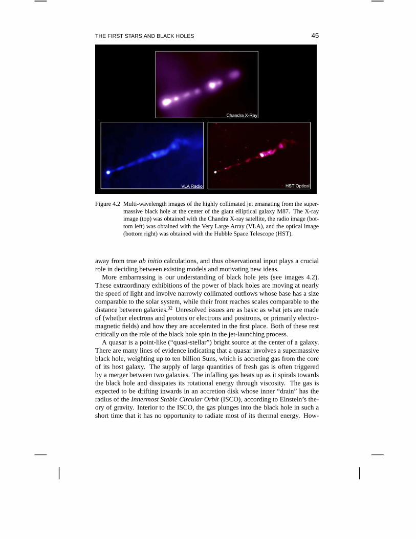
THE FIRST STARS AND BLACK HOLES 45
Figure 4.2 Multi-wavelength images of the highly collimated jet emanating from the super-massive black hole at the center of the giant elliptical galaxy M87. The X-rayimage (top) was obtained with the Chandra X-ray satellite, the radio image (bot-tom left) was obtained with the Very Large Array (VLA), and the optical image(bottom right) was obtained with the Hubble Space Telescope(HST).
away from trueab initio calculations, and thus observational input plays a crucialrole in deciding between existing models and motivating newideas.
More embarrassing is our understanding of black hole jets (see images 4.2).These extraordinary exhibitions of the power of black holesare moving at nearlythe speed of light and involve narrowly collimated outflows whose base has a sizecomparable to the solar system, while their front reaches scales comparable to thedistance between galaxies.32 Unresolved issues are as basic as what jets are madeof (whether electrons and protons or electrons and positrons, or primarily electro-magnetic fields) and how they are accelerated in the first place. Both of these restcritically on the role of the black hole spin in the jet-launching process.
A quasar is a point-like (“quasi-stellar”) bright source atthe center of a galaxy.There are many lines of evidence indicating that a quasar involves a supermassiveblack hole, weighting up to ten billion Suns, which is accreting gas from the coreof its host galaxy. The supply of large quantities of fresh gas is often triggeredby a merger between two galaxies. The infalling gas heats up as it spirals towardsthe black hole and dissipates its rotational energy throughviscosity. The gas isexpected to be drifting inwards in an accretion disk whose inner “drain” has theradius of theInnermost Stable Circular Orbit(ISCO), according to Einstein’s the-ory of gravity. Interior to the ISCO, the gas plunges into theblack hole in such ashort time that it has no opportunity to radiate most of its thermal energy. How-
46 CHAPTER 4
ever, the fraction of the rest mass of the gas which gets radiated away just outsidethe ISCO is high, ranging between 5.7% for a non-spinning black hole to 42% fora maximally-spinning black hole.33 This “radiative efficiency” is far greater thanthe mass-energy conversion efficiency provided by nuclear fusion in stars, which is< 0.7%.
Quasar activity is observed in a small fraction of all galaxies at any cosmic epoch.Mammoth black holes weighing more than a billion solar masses were discoveredat redshifts as high asz ∼ 6.5, less than a billion years after the Big Bang.Ifmassive black holes grow at early cosmic times, should theirremnants be aroundus today?Indeed, searches for black holes in local galaxies have found that everygalaxy with a stellar spheroid harbors a supermassive blackhole at its center. Thisimplies that quasars are rare simply because their activityis short-lived. Moreover,there appears to be a tight correlation between the black hole mass and the grav-itational potential-well depth of their host spheroids of stars (as measured by thevelocity dispersion of these stars). This suggests that theblack holes grow up tothe point where the heat they deposit into their environmentor the piston effectfrom their winds prevent additional gas from feeding them further. The situationis similar to a baby who gets more energetic as he eats more at the dinner table,until his hyper-activity is so intense that he pushes the food off the table and cannoteat any more. Thisprinciple of self-regulationexplains why quasars are short livedand why the final black hole mass is dictated by the depth of thepotential in whichthe gas feeding it resides.34 Most black holes today are dormant or “starved” be-cause the gas around them was mostly used up in making the stars, or because theiractivity heated or pushed it away a long time ago.
What seeded the formation of supermassive black holes only abillion years afterthe Big Bang?We know how to make a black hole out of a massive star. When thestar ends its life, it stops producing sufficient energy to hold itself against its owngravity, and its core collapses to make a black hole. Long before evidence for blackholes was observed, this process leading to their existencewas understood theo-retically by Robert Oppenheimer and Hartland Snyder in 1937. However, growinga supermassive black hole is more difficult. There is a maximum luminosity atwhich the environment of a black hole of massMBH may shine and still accretegas.i This Eddington luminosity,LE, is obtained from balancing the inward forceof gravity on each proton by the outward radiation force on its companion electronat a distancer:
GMBHmp
r2=
LE
4πr2cσT , (4.5)
wheremp is the proton mass andσT = 0.67 × 10⁻²⁴ cm2 is the cross-section
iWhereas the gravitational force acts mostly on the protons,the radiation force acts primarily onthe electrons. These two species are tied together by a global electric field, so that the entire “plasma”(ionized gas) behaves as a single quasi-neutral fluid which is subject to both forces. Under similarcircumstances, electrons are confined to the Sun by an electric potential of about a kilo-Volt (corre-sponding to a total charge of∼ 75 Coulombs). The opposite electric forces per unit volume acting onelectrons and ions in the Sun cancel out so that the total pressure force is exactly balanced by gravity,as for a neutral fluid. An electric potential of 1-10 kilo-Volts also binds electrons to clusters of galaxies(where the thermal velocities of these electrons,∼ 0.1c, are well in excess of the escape speed from thegravitational potential). For a general discussion, see Loeb, A.Phys. Rev.D37, 3484 (1988).
THE FIRST STARS AND BLACK HOLES 47
for scattering a photon by an electron. Interestingly, the limiting luminosity isindependent of radius in the Newtonian regime. Since the Eddington luminosityrepresents an exact balance between gravity and radiation forces, it actually equalsto the luminosity of massive stars which are held at rest against gravity by radiationpressure, as described by equation (4.3). This limit is formally valid in a sphericalgeometry, and exceptions to it were conjectured for other accretion geometries overthe years. But, remarkably, observed quasars for which black hole masses can bemeasured by independent methods appear to respect this limit.
The total luminosity from gas accreting onto a black hole,L, can be written assome radiative efficiencyǫ times the mass accretion rateM ,
L = ǫMc2, (4.6)
with the black hole accreting the non-radiated component,MBH = (1− ǫ)M . Theequation that governs the growth of the black hole mass is then
MBH =MBH
tE, (4.7)
where (after substituting all fundamental constants),
tE = 4 × 10⁷years
(
ǫ/(1 − ǫ)
10%
) (
L
LE
)−1
. (4.8)
We therefore find that as long as fuel is amply supplied, the black hole mass growsexponentially in time,MBH ∝ expt/tE, with ane-folding time tE . Since thegrowth time in equation (4.8) is significantly shorter than the∼ 109 years corre-sponding to the age of the Universe at a redshiftz ∼ 6 – where black holes witha mass∼ 109M⊙ are found, one might naively conclude that there is plenty oftime to grow the observed black hole masses from small seeds.For example, aseed black hole from a Population III star of100M⊙ can grow in less than a billionyears up to∼ 109M⊙ for ǫ ∼ 10% andL ∼ LE . However, the intervention ofvarious processes makes it unlikely that a stellar mass seedwill be able to accretecontinuously at its Eddington limit with no interruption.
For example, mergers are very common in the early Universe. Every time twogas-rich galaxies come together, their black holes are likely to coalesce. The coa-lescence is initially triggered by “dynamical friction” onthe surrounding gas andstars, and is completed – when the binary gets tight – as a result of the emission ofgravitational radiation.35 The existence of gravitational waves is a generic predic-tion of Einstein’s theory of gravity. They represent ripples in space-time generatedby the motion of the two black holes as they move around their common centerof mass in a tight binary. The energy carried by the waves is taken away fromthe kinetic energy of the binary, which therefore gets tighter with time. Computersimulations reveal that when two black holes with unequal masses merge to makea single black hole, the remnant gets a kick due to the non-isotropic emission ofgravitational radiation at the final plunge.ii This kick was calculated recently using
ii The gravitational waves from black hole mergers at high redshifts could in principle be detectedby a proposed space-based mission called theLaser Interferometer Space Antenna(LISA). For moredetails, see http://lisa.nasa.gov/, and, for example, Wyithe, J. S. B., & Loeb, A.Astrophys. J.590, 691(2003).
48 CHAPTER 4
advanced computer codes that solve Einstein’s equations (atask that was plaguedfor decades with numerical instabilities).36 The typical kick velocity is hundredsof kilometer per second (and up to ten times more for special spin orientations),bigger than the escape speed from the first dwarf galaxies.37 This implies that con-tinuous accretion was likely punctuated by black hole ejection events,38 forcing themerged dwarf galaxy to grow a new black hole seed from scratch.iii
If continuous feeding is halted, or if the black hole is temporarily removed fromthe center of its host galaxy, then one is driven to the conclusion that the blackhole seeds must have started more massive than∼ 100M⊙. More massive seedsmay originate from supermassive stars.Is it possible to make such stars in earlygalaxies? Yes, it is. Numerical simulations indicate that stars weighing up toa million Suns could have formed at the centers of early dwarfgalaxies whichwere barely able to cool their gas through transitions of atomic hydrogen, havingTvir ∼ 104K and no H2 molecules. Such systems have a total mass that is severalorders of magnitude higher than the earliest Jeans-mass condensations discussedin §4.1. In both cases, the gas lacks the ability to cool well below Tvir, and so itfragments into one or two major clumps. The simulation shownin Figure 4.3 resultsin clumps of several million solar masses, which inevitablyend up as massive blackholes. The existence of such seeds would have given a jump start to the black holegrowth process.
The nuclear black holes in galaxies are believed to be fed with gas in episodicevents of gas accretion triggered by mergers of galaxies. The energy released bythe accreting gas during these episodes could easily unbindthe gas reservoir fromthe host galaxy and suppress star formation within it. If so,nuclear black holesregulate their own growth by expelling the gas that feeds them. In so doing, theyalso shape the stellar content of their host galaxy. This mayexplain the observedtight correlations between the mass of central black holes in present-day galaxiesand the velocity dispersion39 σ⋆ or luminosity40 Lsp of their host spheroids of stars(namely,MBH ∝ σ4
⋆ or MBH ∝ Lsp). Since the mass of a galaxy at a givenredshift scales with its virial velocity asM ∝ V 3
c in equation (3.11), the bindingenergy of galactic gas is expected to scale asMV 2
c ∝ V 5c while the momentum
required to kick the gas out of its host would scale asMVc ∝ V 4c . Both scalings
can be tuned to explain the observed correlations between black hole masses andthe properties of their host galaxies.41 Star formation inevitably precedes blackhole fueling, since the outer region of the accretion flows that feed nuclear blackholes is typically unstable to fragmentation42. This explains the high abundance ofheavy elements inferred from the broad emission lines of quasars at all redshifts43.
The inflow of cold gas towards galaxy centers during the growth phase of theirblack holes would naturally be accompanied by a burst of starformation. Thefraction of gas not consumed by stars or ejected by supernova-driven winds willcontinue to feed the black hole. It is therefore not surprising that quasar and star-
iii These black hole recoils might have left observable signatures in the local Universe. For example,the halo of the Milky Way galaxy may include hundreds of freely-floating ejected black holes withcompact star clusters around them, representing relics of the early mergers that assembled the MilkyWay out of its original building blocks of dwarf galaxies (O’Leary, R. & Loeb, A.Mon. Not. R. Astron.Soc.395, 781 (2009)).
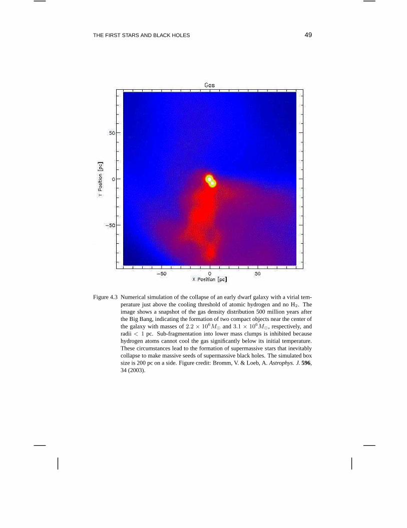
THE FIRST STARS AND BLACK HOLES 49
Figure 4.3 Numerical simulation of the collapse of an early dwarf galaxy with a virial tem-perature just above the cooling threshold of atomic hydrogen and no H2. Theimage shows a snapshot of the gas density distribution 500 million years afterthe Big Bang, indicating the formation of two compact objects near the center ofthe galaxy with masses of2.2 × 106M⊙ and3.1 × 106M⊙, respectively, andradii < 1 pc. Sub-fragmentation into lower mass clumps is inhibited becausehydrogen atoms cannot cool the gas significantly below its initial temperature.These circumstances lead to the formation of supermassive stars that inevitablycollapse to make massive seeds of supermassive black holes.The simulated boxsize is 200 pc on a side. Figure credit: Bromm, V. & Loeb, A.Astrophys. J.596,34 (2003).
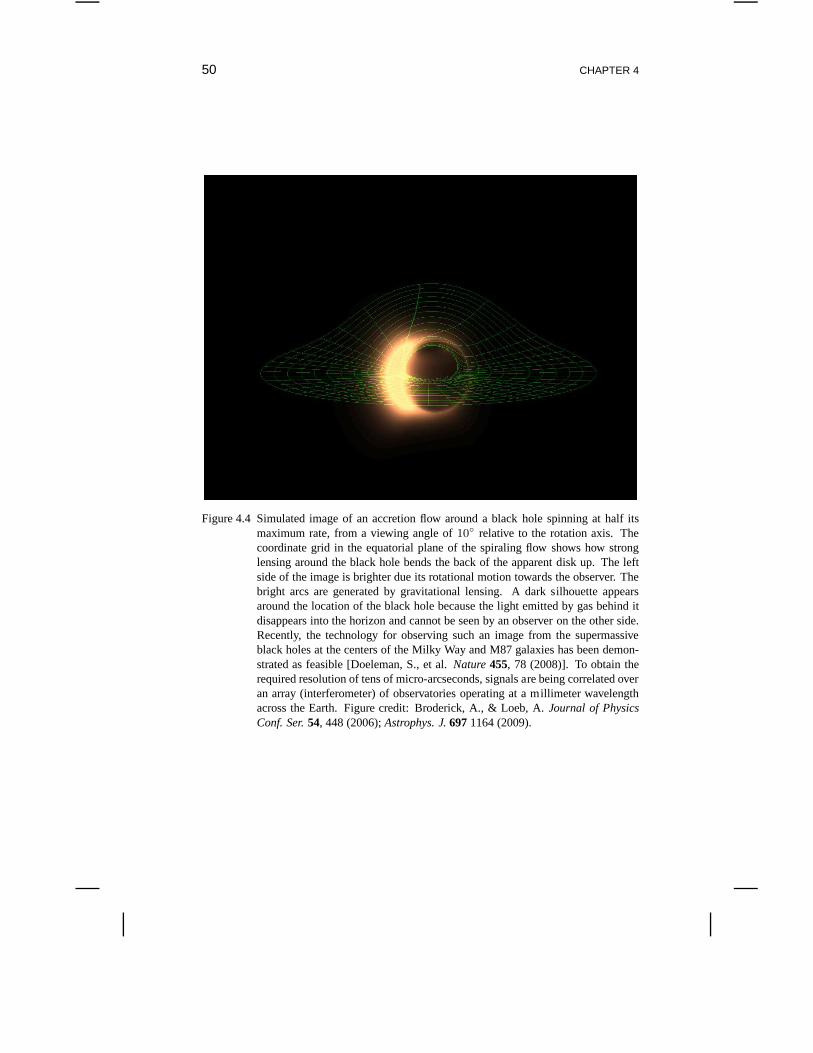
50 CHAPTER 4
Figure 4.4 Simulated image of an accretion flow around a blackhole spinning at half itsmaximum rate, from a viewing angle of10 relative to the rotation axis. Thecoordinate grid in the equatorial plane of the spiraling flowshows how stronglensing around the black hole bends the back of the apparent disk up. The leftside of the image is brighter due its rotational motion towards the observer. Thebright arcs are generated by gravitational lensing. A dark silhouette appearsaround the location of the black hole because the light emitted by gas behind itdisappears into the horizon and cannot be seen by an observeron the other side.Recently, the technology for observing such an image from the supermassiveblack holes at the centers of the Milky Way and M87 galaxies has been demon-strated as feasible [Doeleman, S., et al.Nature455, 78 (2008)]. To obtain therequired resolution of tens of micro-arcseconds, signals are being correlated overan array (interferometer) of observatories operating at a millimeter wavelengthacross the Earth. Figure credit: Broderick, A., & Loeb, A.Journal of PhysicsConf. Ser.54, 448 (2006);Astrophys. J.6971164 (2009).
THE FIRST STARS AND BLACK HOLES 51
burst activities co-exist in ultra-luminous galaxies, andthat all quasars show strongspectral lines of heavy elements. Similarly to the above-mentioned prescription formodelling galaxies, it is possible to “dress up” the mass distribution of halos inFigure 3.2 with quasar luminosities (related toLE , which is a prescribed functionof M based on the observedMBH–σ⋆ relation) and a duty cycle (related totE), andfind the evolution of the quasar population over redshift. This simple approach canbe tuned to give good agreement with existing data on quasar evolution.44
The early growth of massive black holes led to the supermassive black holesobserved today. In our own Milky Way galaxy, stars are observed to zoom aroundthe Galactic center at speeds of up to ten thousand kilometers per second, owingto the strong gravitational acceleration near the central black hole.45 But closer-inobservations are forthcoming. Existing technology shouldsoon be able to imagethe silhouette of the supermassive black holes in the Milky Way and M87 galaxiesdirectly (see Figure 4.4).
4.4 GAMMA-RAY BURSTS: THE BRIGHTEST EXPLOSIONS
Gamma-ray bursts (GRBs) were discovered in the late 1960s bythe American Velasatellites, built to search for flashes of high energy photons (“gamma rays”) fromSoviet nuclear weapon tests in space. The United States suspected that the Sovietsmight attempt to conduct secret nuclear tests after signingthe Nuclear Test BanTreaty in 1963. On July 2, 1967, the Vela 4 and Vela 3 satellites detected a flashof gamma radiation unlike any known nuclear weapons signature. Uncertain ofits meaning but not considering the matter particularly urgent, the team at the LosAlamos Laboratory, led by Ray Klebesadel, filed the data awayfor future inves-tigation. As additional Vela satellites were launched withbetter instruments, theLos Alamos team continued to find unexplained GRBs in their data. By analyzingthe different arrival times of the bursts as detected by different satellites, the teamwas able to estimate the sky positions of 16 bursts and definitively rule out eithera terrestrial or solar origin. The discovery was declassified and published in 1973(Astrophys. J.182, L85) under the title “Observations of Gamma-Ray Bursts ofCosmic Origin.”
The distance scale and nature of GRBs remained mysterious for more than twodecades. Initially, astronomers favored a local origin forthe bursts, associatingthem with sources within the Milky Way. In 1991, the Compton Gamma Ray Ob-servatory satellite was launched, and its “Burst and Transient Source Explorer”instrument started to discover a GRB every day or two, increasing the total num-ber of known GRBs up to a few thousand. The larger statisticalsample of GRBsmade it evident that their distribution on the sky is isotropic. Such a distributionwould be most natural if the bursts originate at cosmological distances since theUniverse is the only system which is truly isotropic around us. Nevertheless, thelocal origin remained more popular within the GRB communityfor six years, untilFebruary 1997, when the Italian-Dutch satellite BeppoSAX detected a gamma-rayburst (GRB 970228) and localized it to within minutes of arc using its X-ray cam-era. With this prompt localization, ground-based telescopes were able to identify a
52 CHAPTER 4
fading counterpart in the optical band. Once the GRB afterglow faded, deep imag-ing revealed a faint, distant host galaxy at the location of the optical afterglow of theGRB. The association of a host galaxy at a cosmological distance for this burst andmany subsequent ones revised the popular view in favor of associating GRBs withcosmological distances. This shift in popular view provides testimony to how apsychological bias in the scientific community can be overturned by hard scientificevidence.46
A GRB afterglow is initially brightest at short photon wavelengths and then fadesaway at longer wavelengths, starting in the X-ray band (overtimescales of minutesto hours), shifting to the UV and optical band (over days), and ending in the infraredand radio (over weeks and months).iv Among the first detected afterglows, ob-servers noticed that as the afterglow lightcurve faded, long-duration GRBs showedevidence for a supernova flare, indicating that they are alsoassociated with core-collapse supernova events. The associated supernovae wereclassified as relatedto massive stars which have lost their hydrogen envelope in awind. In addition,long-duration GRBs were found to be associated with star-forming regions wheremassive stars form and explode only a million years after being born. These cluesindicated that long-duration GRBs are most likely associated with massive stars.The most popular model for long-duration GRBs became known as the “collapsar”model47 (see illustration 4.5). According to this model, the progenitor of the GRBis a massive star whose core eventually consumes its nuclearfuel, loses pressuresupport, and collapses. If the core of the star is too massiveto make a neutron star,it collapses to a black hole. As material is spiraling into the black hole, two jetsare produced at a speed close to that of light. So far, there isnothing spectacularabout this setting, since we see scaled-up versions of such jets being formed aroundmassive black holes in the centers of galaxies, as shown in Figure 4.2. However,when jets are generated in the core of a star, they have to maketheir way out bydrilling a hole in the surrounding dense envelope. As soon asthe head of a jetexits, the highly collimated stream of radiation emanatingfrom it would appear asa gamma-ray flash to an observer who happened to line up with its jet axis. Thesubsequent afterglow results from the interaction betweenthe jet and the ambientgas in the vicinity of the progenitor star. As the jet slows down by pushing againstthe ambient medium, the non-thermal radiation from accelerated relativistic elec-trons in the shock wave in front of it gets shifted to longer wavelengths and fainterluminosities. Also, as the jet makes its way out of the star, its piston effect depositsenergy in the stellar envelope and explodes the star, supplementing the GRB witha supernova-like explosion. Because of their immense luminosities, GRBs can beobserved out to the edge of the Universe. These bright signals may be thought of asthe cosmic fireworks signaling the birth of black holes at theend of the life of theirparent massive stars. If the first stars produced GRBs (as their descendants do in themore recent Universe), then they would be detectable out to their highest redshifts.Their powerful beacons of light can be used to illuminate thedark ages and probethe cosmic gas around the time when it condensed to make the first galaxies. As
ivFor an extreme example of a GRB afterglow from a redshiftz = 0.94 that was bright enough tobe seen with the naked eye, see Bloom, J., et al.Astrophys. J.691, 723 (2009).
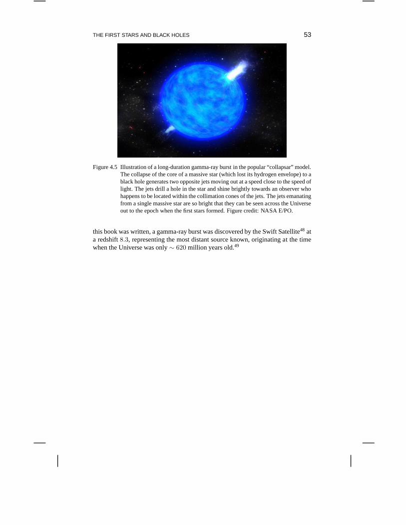
THE FIRST STARS AND BLACK HOLES 53
Figure 4.5 Illustration of a long-duration gamma-ray burstin the popular “collapsar” model.The collapse of the core of a massive star (which lost its hydrogen envelope) to ablack hole generates two opposite jets moving out at a speed close to the speed oflight. The jets drill a hole in the star and shine brightly towards an observer whohappens to be located within the collimation cones of the jets. The jets emanatingfrom a single massive star are so bright that they can be seen across the Universeout to the epoch when the first stars formed. Figure credit: NASA E/PO.
this book was written, a gamma-ray burst was discovered by the Swift Satellite48 ata redshift8.3, representing the most distant source known, originating at the timewhen the Universe was only∼ 620 million years old.49

Chapter Five
The Reionization of Cosmic Hydrogen by the First
Galaxies
5.1 IONIZATION SCARS BY THE FIRST STARS
The cosmic microwave background (CMB) indicates that hydrogen atoms formed400 thousand years after the Big Bang, as soon as the gas cooled below 3,000K asa result of cosmological expansion. Observations of the spectra of early galaxies,quasars, and gamma-ray bursts indicate that less than a billion years later the samegas underwent a wrenching transition from atoms back to their constituent protonsand electrons in a process known as reionization. Indeed, the bulk of the Uni-verse’s ordinary matter today is in the form of free electrons and protons, locateddeep in intergalactic space. The free electrons have other side effects; for example,they scatter the CMB and produce polarization fluctuations at large angles on thesky.i The latest analysis of the CMB polarization data from WMAP50 indicates that8.7±1.7% of the CMB photons were scattered by free electrons after cosmologicalrecombination, implying that reionization took place at around a redshiftz ∼ 10,only 500 million years after the Big Bang.ii It is intriguing that the inferred reion-ization epoch coincides with the appearance of the first galaxies, which inevitablyproduced ionizing radiation.How was the primordial gas transformed to an ionizedstate by the first galaxies within merely hundreds of millionof years?
We can address this question using the results of§3 & §4 concerning the for-mation rate of new galaxies at various cosmic epochs. The course of reionizationcan be determined by counting photons from all galaxies as a function of time.Both stars and black holes contribute ionizing photons, butthe early Universe isdominated by small galaxies which, in the local universe, have disproportionatelysmall central black holes. In fact, bright quasars are knownto be extremely rare
iPolarization is produced when free electrons scatter a radiation field with a quadrupole anisotropyQ. Consequently, reionization generates a fractional CMB polarization of P ∼ 0.1τQ out of theCMB quadrupole on scales of the horizon at reionization. Here, τ =
R zreion
0ne(z)σT (cdt/dz)dz
is the optical depth for scattering by electrons of mean density ne(z), which provides a measure ofthe redshift of reionization,zreion. (The scattering probability,τ ≪ 1, is the chance that a photonwill encounter an electron within the volume associated with the scattering cross-sectionσT times thephoton path length
R
cdt.) For a sudden reionization of hydrogen and neutral helium at redshiftzreion,τ = 4.75 × 10⁻³ × [ΩΛ + Ωm(1 + zreion)3]1/2 − 1.
ii This number will be refined by forthcoming CMB data from the Planck satellite(http://www.rssd.esa.int/index.php?project=planck),and will be supplemented by constraints from21-cm observations as described in§7 [see Pritchard, J., Loeb, A., & Wyithe, J. S. B.,http://arxiv.org/abs/0908.3891 (2009)].
56 CHAPTER 5
above redshift 6, indicating that stars most likely dominated the production of ion-izing UV photons during the reionization epoch.51 Since stellar ionizing photonsare only slightly more energetic than the 13.6 eV ionizationthreshold of hydro-gen, they are absorbed efficiently once they reach a region with substantial neutralhydrogen. This makes the inter-galactic medium (IGM) during reionization a two-phase medium characterized by highly ionized regions separated from neutral re-gions by sharp ionization fronts. We can obtain a first estimate of the requirementsof reionization by demanding one stellar ionizing photon for each hydrogen atomin the Universe. As discussed in§4.2, if we conservatively assume that stars withinthe early galaxies were similar to those observed locally, then each star produced∼ 4, 000 ionizing photons per proton in it. Star formation is observed today to bean inefficient process, but even if stars in galaxies formed out of only a fractionf⋆ ∼ 10% of the available gas, this amount was still sufficient to assemble only asmall fraction of the total mass in the universe into galaxies in order to ionize theentire IGM. This fraction would be∼ 2.5%(fesc/10%)−1 for an escape fractionfesc of ionizing UV photons out of galaxies. More detailed estimates of the ac-tual required fraction account for the formation of some Population III stars (whichwere more efficient ionizers, as discussed in§4), and for recombinations of hydro-gen atoms at high redshifts and in dense regions. At the mean IGM density, therecombination time of hydrogen is shorter than the age of theUniverse atz > 8.
From studies of the processed spectra of quasars atz ∼ 6, we know that theIGM is highly ionized a billion years after the Big Bang. There are hints, however,that some large neutral hydrogen regions persist at these early times which suggeststhat we may not need to go to much higher redshifts to begin to see the epoch ofreionization. We now know that the universe could not have fully reionized earlierthan an age of 300 million years, since WMAP observed the effect of the freshlycreated plasma at reionization on the large-scale polarization anisotropies of theCMB which limits the reionization redshift; an earlier reionization, when the uni-verse was denser, would have created a stronger scattering signature that wouldhave been inconsistent with the WMAP observations. In any case, the redshift atwhich reionization ended only constrains the overall cosmic efficiency for produc-ing ionizing photons. In comparison, a detailed picture of reionization in progresswill teach us a great deal about the population of the first galaxies that producedthis cosmic phase transition.
5.2 PROPAGATION OF IONIZATION FRONTS
Astronomers label the neutral and singly ionized states of an atomic species as Iand II; for example, abbreviating neutral hydrogen as H I andionized hydrogenas H II. The radiation output from the first stars ionizes H I ina growing volume,eventually encompassing almost the entire IGM within a single H II bubble. Inthe early stages of this process, each galaxy produced a distinct H II region, andonly when the overall H II filling factor became significant did neighboring bubblesbegin to overlap in large numbers, ushering in the “overlap phase” of reionization.Thus, the first goal of a model of reionization is to describe the initial stage, during
THE REIONIZATION OF COSMIC HYDROGEN BY THE FIRST GALAXIES 57
which each source produces an isolated expanding H II region.Let us consider, for simplicity, a spherical ionized volumeV , separated from the
surrounding neutral gas by a sharp ionization front. In the absence of recombina-tions, each hydrogen atom in the IGM would only have to be ionized once, and theionized physical volumeVp would simply be determined by
nHVp = Nγ , (5.1)
wherenH is the mean number density of hydrogen andNγ is the total number ofionizing photons produced by the source. However, the elevated density of the IGMat high redshift implies that recombinations cannot be ignored. Just before WorldWar II, the Danish astronomer Bengt Stromgren analyzed thesame problem for hotstars embedded in the interstellar medium.52 In the case of a steady ionizing source(and neglecting the cosmological expansion), he found thata steady-state volume(now termed a ‘Stromgren Sphere’) would be reached, through which recombina-tions are balancing ionizations:
αBn2HVp =
dNγ
dt, (5.2)
where the recombination rate depends on the square of the density and on the re-combination coefficientiii (to all states except the ground energy level, which wouldjust recycle the ionizing photon)αB = 2.6 × 10⁻¹³ cm3 s−1 for hydrogen atT = 104 K. The complete description of the evolution of an expandingH II re-gion, including the ingredients of a non-steady ionizing source, recombinations,and cosmological expansion, is given by53
nH
(
dVp
dt− 3HVp
)
=dNγ
dt− αB
⟨
n2H
⟩
Vp . (5.3)
In this equation, the mean densitynH varies with time as1/a3(t). Note that therecombination rate scales as the square of the density. Therefore, if the IGM isnot uniform, but instead the gas which is being ionized is mostly distributed inhigh-density clumps, then the recombination time will be shorter. This is oftenaccommodated for by introducing a volume-averaged clumping factorC (which is,in general, time dependent), defined byiv
C =⟨
n2H
⟩
/n2H . (5.4)
If the ionized volume is large compared to the typical scale of clumping, so thatmany clumps are averaged over, then equation (5.3) can be solved by supplement-ing it with equation (5.4) and specifyingC. Switching to the comoving volumeV ,the resulting equation is
dV
dt=
1
n0H
dNγ
dt− αB
C
a3n0
HV , (5.5)
where the present number density of hydrogen is
n0H = 2.1 × 10⁻⁷ cm−3 . (5.6)
iii See§2 in Osterbrock, D. E., & Ferland, G. J.Astrophysics of Gaseous Nebulae and Active GalacticNuclei, University Science Books, Sausalito (2006).
ivThe recombination rate depends on the number density of electrons, and in using equation (5.4)we are neglecting the small contribution made by partially or fully ionized helium.
58 CHAPTER 5
This number density is lower than the total number density ofbaryonsn0b by a
factor of∼ 0.76, corresponding to the primordial mass fraction of hydrogen. Thesolution forV (t) around a source which turns on att = ti is 54
V (t) =
∫ t
ti
1
n0H
dNγ
dt′eF (t′,t)dt′ , (5.7)
where
F (t′, t) = −αBn0H
∫ t
t′
C(t′′)
a3(t′′)dt′′ . (5.8)
At high redshifts (z ≫ 1), the scale factor varies as
a(t) ≃(
3
2
√
ΩmH0t
)2/3
, (5.9)
and with the additional assumption of a constantC, the functionF simplifies asfollows. Defining
f(t) = a(t)−3/2 , (5.10)
we derive
F (t′, t) = −2
3
αBn0H√
ΩmH0
C [f(t′) − f(t)] = −0.26
(
C
10
)
[f(t′) − f(t)] . (5.11)
The size of the resulting H II region depends on the halo whichproduces it. Letus consider a halo of total massM and baryon fractionΩb/Ωm. To derive a roughestimate, we assume that baryons are incorporated into stars with an efficiency off⋆ = 10%, and that the escape fraction for the resulting ionizing radiation is alsofesc = 10%. As mentioned in§4, Population II stars produce a total ofNγ ≈ 4, 000ionizing photons per baryon in them. We may define a parameterwhich gives theoverall number of ionizations per baryon,
Nion ≡ Nγ f⋆ fesc . (5.12)
If we neglect recombinations then we obtain the maximum comoving radius of theregion which the halo of massM can ionize as,
rmax =
(
3
4π
Nγ
n0H
)1/3
=
(
3
4π
Nion
n0H
Ωb
Ωm
M
mp
)1/3
= 680 kpc
(
Nion
40
M
108M⊙
)1/3
.
(5.13)However, the actual radius never reaches this size if the recombination time isshorter than the lifetime of the ionizing source.
We may obtain a similar estimate for the size of the H II regionaround a galaxy ifwe consider a quasar rather than stars. For the typical quasar spectrum,∼ 104 ion-izing photons are produced per baryon incorporated into theblack hole, assuming aradiative efficiency of∼ 6%. The overall efficiency of incorporating the collapsedfraction of baryons into the central black hole is low (< 0.01% in the local Uni-verse), butfesc is likely to be close to unity for powerful quasars which ionize theirhost galaxy. If we take the limit of an extremely bright source, characterized by anarbitrarily high production rate of ionizing photons, thenequation 5.3 would imply
THE REIONIZATION OF COSMIC HYDROGEN BY THE FIRST GALAXIES 59
that the H II region expands faster than light. This result isclearly unphysical andmust be corrected for bright sources. At early times, the ionization front arounda bright quasar would have expanded at nearly the speed of light, c, but this onlyoccurs when the H II region is sufficiently small such that theproduction rate ofionizing photons by the central source exceeds their consumption rate by hydrogenatoms within this volume. It is straightforward to do the accounting for these rates(including recombination) by taking the light propagationdelay into account. Thegeneral equation for the relativistic expansion of thecomovingradiusr = (1+z)rp
of a quasar H II region in an IGM with neutral filling fractionxHI (fixed by otherionizing sources) is given by55,
dr
dt= c(1 + z)
[
Nγ − αBCxHI
(
n0H
)2(1 + z)
3 (
4π3 r3
)
Nγ + 4πr2 (1 + z) cxHIn0H
]
, (5.14)
whereNγ is the rate of ionizing photons crossing a shell of the H II region atradiusr and timet. Indeed, forNγ → ∞ the propagation speed of the physicalradius of the H II regionrp = r/(1 + z) approaches the speed of light in the aboveexpression,(drp/dt) → c.
The process of the reionization of hydrogen involves several distinct stages.56
The initial “pre-overlap” stage consists of individual ionizing sources turning onand ionizing their surroundings. The first galaxies form in the most massive ha-los at high redshift, which are preferentially located in the highest-density regions.Thus, the ionizing photons which escape from the galaxy itself must then maketheir way through the surrounding high-density regions, characterized by a highrecombination rate. Once they emerge, the ionization fronts propagate more easilythrough the low-density voids, leaving behind pockets of neutral, high-density gas.During this period, the IGM is a two-phase medium characterized by highly ion-ized regions separated from neutral regions by ionization fronts. Furthermore, theionizing intensity is very inhomogeneous even within the ionized regions.
The central, relatively rapid “overlap” phase of reionization begins when neigh-boring H II regions begin to overlap. Whenever two ionized bubbles are joined,each point inside their common boundary becomes exposed to ionizing photonsfrom both sources. Therefore, the ionizing intensity inside H II regions rises rapidly,allowing those regions to expand into high-density gas which had previously re-combined fast enough to remain neutral when the ionizing intensity had been low.Since each bubble coalescence accelerates the process of reionization, the overlapphase has the character of a phase transition and is expectedto occur rapidly. Bythe end of this stage, most regions in the IGM are able to “see”several unobscuredsources, therefore the ionizing intensity is much higher and more homogeneousthan before overlap. An additional attribute of this rapid “overlap” phase resultsfrom the fact that hierarchical structure formation modelspredict a galaxy forma-tion rate that rises rapidly with time at these high redshifts. This is because mostgalaxies fall on the exponential tail of the Press-Schechter mass function at earlycosmic times, and so the fraction of mass that gets incorporated into stars growsexponentially with time. This process leads to a final state in which the low-densityIGM has been highly ionized, with ionizing radiation reaching everywhere except
60 CHAPTER 5
gas located inside self-shielded, high-density clouds. This “moment of reioniza-tion” marks the end of the “overlap phase.”
Some neutral gas does, however, remain in high-density structures, which aregradually ionized as galaxy formation proceeds and the meanionizing intensitygrows with time. The ionizing intensity continues to grow and become more uni-form as an increasing number of ionizing sources is visible to every point in theIGM.
Analytic models of the pre-overlap stage focus on the evolution of the H II fillingfactor, i.e., the fraction of the volume of the Universe which is filled by H II regions,QH II. The modelling of individual H II regions can be used to understand thedevelopment of the total filling factor. Starting with equation (5.5), if we assumea common clumping factorC for all H II regions, then we can sum each term ofthe equation over all bubbles in a given large volume of the Universe and thendivide by this volume. ThenV can be replaced by the filling factor andNγ bythe total number of ionizing photons produced up to some timet, per unit volume.The latter quantitynγ equals the mean number of ionizing photons per baryonmultiplied by the mean density of baryonsnb. Following the arguments leading toequation (5.13), we find that if we include only stars
nγ
nb= NionFcol , (5.15)
where the collapse fractionFcol is the fraction of all the baryons in the Universewhich are in galaxies, i.e., the fraction of gas which has settled into halos and cooledefficiently inside them. In writing equation (5.15) we are assuming instantaneousproduction of photons, i.e., that the timescale for the formation and evolution ofthe massive stars in a galaxy is relatively short compared tothe Hubble time at theformation redshift of the galaxy. The total number of ionizations equals the totalnumber of ionizing photons produced by stars, i.e., all ionizing photons contributeregardless of the spatial distribution of sources. Also, the total recombination rateis proportional to the total ionized volume, regardless of its topology. Thus, evenif two or more bubbles overlap, the model remains a good first approximation forQH II (at least until its value approaches unity).
Under these assumptions we convert equation (5.5), which describes individualH II regions, to an equation which statistically describes the transition from a neu-tral Universe to a fully ionized one:
dQH II
dt=
Nion
0.76
dFcol
dt− αB
C
a3n0
HQH II , (5.16)
which admits the solution (in analogy with equation 5.7),
QH II(t) =
∫ t
0
Nion
0.76
dFcol
dt′eF (t′,t)dt′ , (5.17)
whereF (t′, t) is determined by equation (5.11).A simple estimate of the collapse fraction at high redshift is the mass fraction
(given by equation (3.17) in the Press-Schechter model) in halos above the coolingthreshold, which gives the minimum mass of halos in which gascan cool effi-ciently. Assuming that only atomic cooling is effective during the redshift range of
THE REIONIZATION OF COSMIC HYDROGEN BY THE FIRST GALAXIES 61
reionization, the minimum mass corresponds roughly to a halo of virial temperatureTvir = 104 K, which can be converted to a mass using equation (3.12).
Although many models yield a reionization redshift aroundz ∼ 10, the exactvalue depends on a number of uncertain parameters affectingboth the source termand the recombination term in equation (5.16). The source parameters include theformation efficiency of stars and quasars and the escape fraction of ionizing photonsproduced by these sources.
The overlap of H II regions is expected to have occurred at different times in dif-ferent regions of the IGM due to the cosmic scatter during theprocess of structureformation within finite spatial volumes. Reionization should be completed within aregion of comoving radiusR when the fraction of mass incorporated into collapsedobjects in this region attains a certain critical value, corresponding to a thresholdnumber of ionizing photons emitted per baryon. The ionization state of a regionis governed by the factors of its enclosed ionizing luminosity, its over-density, anddense pockets of neutral gas within the region that are self shielding to ionizingradiation. There is an offsetδz between the redshift at which a region of meanover-densityδR achieves this critical collapsed fraction, and the redshift z at whichthe Universe achieves the same collapsed fraction on average. This offset may becomputed57 from the expression for the collapsed fractionFcol within a region ofover-densityδR on a comoving scaleR, within the excursion-set formalism de-scribed in§4, giving
Fcol = erfc
δcrit − δR√
2[σ2Rmin
− σ2R]
→ δz
(1 + z)=
δR
δcrit(z)−
[
1 −√
1 − σ2R
σ2Rmin
]
,
(5.18)whereδcrit(z) ∝ (1 + z) is the collapse threshold for an over-density at a redshiftz; andσR andσRmin
are the variances in the power spectrum linearly extrapolatedto z = 0 on comoving scales corresponding to the region of interest and to theminimum galaxy massMmin, respectively. The offset in the ionization redshift of aregion depends on its linear over-densityδR. As a result, the distribution of offsetsmay be obtained directly from the power spectrum of primordial inhomogeneities.As can be seen from equation (5.18), larger regions have a smaller scatter due totheir smaller cosmic variance. Interestingly, equation (5.18) is independent of thecritical value of the collapsed fraction required for reionization.
The size distribution of ionized bubbles can also be calculated with an approxi-mate analytic approach based on the excursion set formalism.58 For a region to beionized, galaxies inside it must produce a sufficient numberof ionizing photons perbaryon. This condition can be translated to the requirementthat the collapsed frac-tion of mass in halos above some minimum massMmin will exceed some threshold,namelyFcol > ζ−1. For example, requiring one ionizing photon per baryon wouldcorrespond to settingζ = Nion, whereNion is defined in equation (5.12). Wewould like to find the largest region around every point whosecollapse fraction sat-isfies the above condition on the collapse fraction, then calculate the abundance ofionized regions of this size. Different regions have different values ofFcol becausetheir mean density is different. Writing the collapse fraction in a region of mean
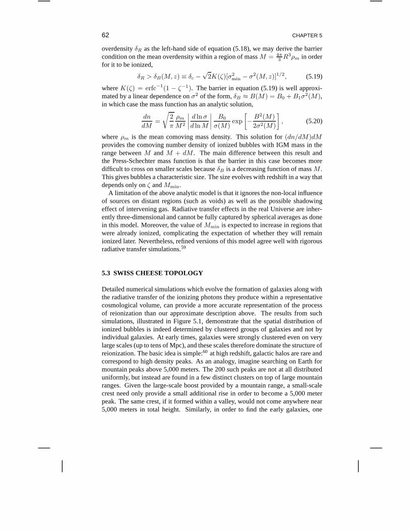
62 CHAPTER 5
overdensityδR as the left-hand side of equation (5.18), we may derive the barriercondition on the mean overdensity within a region of massM = 4π
3 R3ρm in orderfor it to be ionized,
δR > δB(M, z) ≡ δc −√
2K(ζ)[σ2min − σ2(M, z)]1/2, (5.19)
whereK(ζ) = erfc−1(1 − ζ−1). The barrier in equation (5.19) is well approxi-mated by a linear dependence onσ2 of the form,δB ≈ B(M) = B0 + B1σ
2(M),in which case the mass function has an analytic solution,
dn
dM=
√
2
π
ρm
M2
∣
∣
∣
∣
d lnσ
d lnM
∣
∣
∣
∣
B0
σ(M)exp
[
− B2(M)
2σ2(M)
]
, (5.20)
whereρm is the mean comoving mass density. This solution for(dn/dM)dMprovides the comoving number density of ionized bubbles with IGM mass in therange betweenM and M + dM . The main difference between this result andthe Press-Schechter mass function is that the barrier in this case becomes moredifficult to cross on smaller scales becauseδB is a decreasing function of massM .This gives bubbles a characteristic size. The size evolves with redshift in a way thatdepends only onζ andMmin.
A limitation of the above analytic model is that it ignores the non-local influenceof sources on distant regions (such as voids) as well as the possible shadowingeffect of intervening gas. Radiative transfer effects in the real Universe are inher-ently three-dimensional and cannot be fully captured by spherical averages as donein this model. Moreover, the value ofMmin is expected to increase in regions thatwere already ionized, complicating the expectation of whether they will remainionized later. Nevertheless, refined versions of this modelagree well with rigorousradiative transfer simulations.59
5.3 SWISS CHEESE TOPOLOGY
Detailed numerical simulations which evolve the formationof galaxies along withthe radiative transfer of the ionizing photons they producewithin a representativecosmological volume, can provide a more accurate representation of the processof reionization than our approximate description above. The results from suchsimulations, illustrated in Figure 5.1, demonstrate that the spatial distribution ofionized bubbles is indeed determined by clustered groups ofgalaxies and not byindividual galaxies. At early times, galaxies were strongly clustered even on verylarge scales (up to tens of Mpc), and these scales therefore dominate the structure ofreionization. The basic idea is simple:60 at high redshift, galactic halos are rare andcorrespond to high density peaks. As an analogy, imagine searching on Earth formountain peaks above 5,000 meters. The 200 such peaks are notat all distributeduniformly, but instead are found in a few distinct clusters on top of large mountainranges. Given the large-scale boost provided by a mountain range, a small-scalecrest need only provide a small additional rise in order to become a 5,000 meterpeak. The same crest, if it formed within a valley, would not come anywhere near5,000 meters in total height. Similarly, in order to find the early galaxies, one
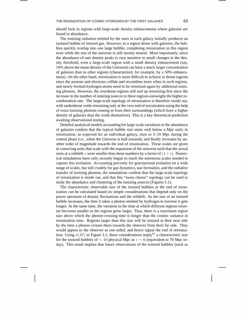
THE REIONIZATION OF COSMIC HYDROGEN BY THE FIRST GALAXIES 63
should look in regions with large-scale density enhancements where galaxies arefound in abundance.
The ionizing radiation emitted by the stars in each galaxy initially produces anisolated bubble of ionized gas. However, in a region dense with galaxies, the bub-bles quickly overlap into one large bubble, completing reionization in this regioneven while the rest of the universe is still mostly neutral. Most importantly, sincethe abundance of rare density peaks is very sensitive to small changes in the den-sity threshold, even a large-scale region with a small density enhancement (say,10% above the mean density of the Universe) can have a much larger concentrationof galaxies than in other regions (characterized, for example, by a 50% enhance-ment). On the other hand, reionization is more difficult to achieve in dense regionssince the protons and electrons collide and recombine more often in such regions,and newly-formed hydrogen atoms need to be reionized again by additional ioniz-ing photons. However, the overdense regions still end up reionizing first since theincrease in the number of ionizing sources in these regions outweighs the higher re-combination rate. The large-scale topology of reionization is thereforeinside out,with underdense voids reionizing only at the very end of reionization using the helpof extra ionizing photons coming in from their surroundings(which have a higherdensity of galaxies than the voids themselves). This is a keytheoretical predictionawaiting observational testing.
Detailed analytical models accounting for large-scale variations in the abundanceof galaxies confirm that the typical bubble size starts well below a Mpc early inreionization, as expected for an individual galaxy, rises to 5–10 Mpc during thecentral phase (i.e., when the Universe is half-ionized), and finally increases by an-other order of magnitude towards the end of reionization. These scales are givenin comoving units that scale with the expansion of the universe such that the actualsizes at a redshiftz were smaller than these numbers by a factor of(1+z). Numer-ical simulations have only recently begun to reach the enormous scales needed tocapture this evolution. Accounting precisely for gravitational evolution on a widerange of scales, but still crudely for gas dynamics, star formation, and the radiativetransfer of ionizing photons, the simulations confirm that the large-scale topologyof reionization is inside out, and that this “swiss cheese” topology can be used tostudy the abundance and clustering of the ionizing sources (Figures 5.1).
The characteristic observable size of the ionized bubbles at the end of reion-ization can be calculated based on simple considerations that depend only on thepower spectrum of density fluctuations and the redshift. As the size of an ionizedbubble increases, the time it takes a photon emitted by hydrogen to traverse it getslonger. At the same time, the variation in the time at which different regions reion-ize becomes smaller as the regions grow larger. Thus, there is a maximum regionsize above which the photon-crossing time is longer than thecosmic variance inreionization time. Regions larger than this size will be ionized at their near sideby the time a photon crosses them towards the observer from their far side. Theywould appear to the observer as one-sided, and hence signal the end of reioniza-tion. Usingσ(M) in Figure 3.1, these considerations imply61 a characteristic sizefor the ionized bubbles of∼ 10 physical Mpc atz ∼ 6 (equivalent to 70 Mpc to-day). This result implies that future observations of the ionized bubbles (such as
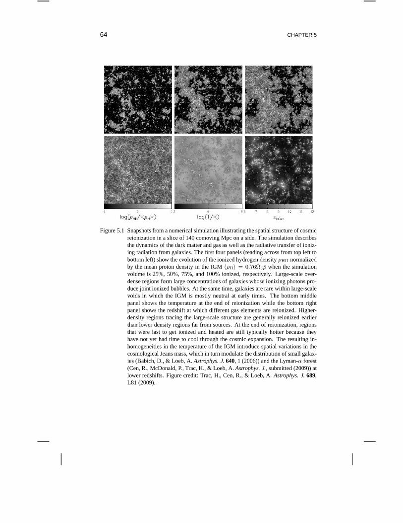
64 CHAPTER 5
Figure 5.1 Snapshots from a numerical simulation illustrating the spatial structure of cosmicreionization in a slice of 140 comoving Mpc on a side. The simulation describesthe dynamics of the dark matter and gas as well as the radiative transfer of ioniz-ing radiation from galaxies. The first four panels (reading across from top left tobottom left) show the evolution of the ionized hydrogen density ρHII normalizedby the mean proton density in the IGM〈ρH〉 = 0.76Ωb ρ when the simulationvolume is 25%, 50%, 75%, and 100% ionized, respectively. Large-scale over-dense regions form large concentrations of galaxies whose ionizing photons pro-duce joint ionized bubbles. At the same time, galaxies are rare within large-scalevoids in which the IGM is mostly neutral at early times. The bottom middlepanel shows the temperature at the end of reionization whilethe bottom rightpanel shows the redshift at which different gas elements arereionized. Higher-density regions tracing the large-scale structure are generally reionized earlierthan lower density regions far from sources. At the end of reionization, regionsthat were last to get ionized and heated are still typically hotter because theyhave not yet had time to cool through the cosmic expansion. The resulting in-homogeneities in the temperature of the IGM introduce spatial variations in thecosmological Jeans mass, which in turn modulate the distribution of small galax-ies (Babich, D., & Loeb, A.Astrophys. J.640, 1 (2006)) and the Lyman-α forest(Cen, R., McDonald, P., Trac, H., & Loeb, A.Astrophys. J., submitted (2009)) atlower redshifts. Figure credit: Trac, H., Cen, R., & Loeb, A.Astrophys. J.689,L81 (2009).

THE REIONIZATION OF COSMIC HYDROGEN BY THE FIRST GALAXIES 65
the low-frequency radio experiments described in§6) should be tuned to a charac-teristic angular scale of tens of arcminutes for an optimal detection of brightnessfluctuations in the emission of hydrogen near the end of reionization.

Chapter Six
Observing the First Galaxies
6.1 THEORIES AND OBSERVATIONS
A couple of years ago, my family and I visited the remote island of Tasmania off thecoast of Australia, known for its unspoiled natural environment. Upon our arrivalat a secluded lodge near the beautiful Cradle Mountain reserve, I discovered therewas no internet connectivity. When night settled in, I had a few hours to spare – thetime I ordinarily use to answer e-mails and check the daily postings of papers on theastro-ph web archive. I stepped out of our cabin and looked around at the pristinesight of nature left to its own. The night was dark with no citylight anywhere on thehorizon. Up on the sky was a magnificent view of the Milky Way galaxy stretchedout in its full glory on a black background. For hours, I stared at our Galaxy’s stars,dust, globular clusters, Magellanic clouds, as well as its sister galaxy - Andromeda,realizing at a deeper level that what we astronomers talk about truly exists outthere. Eighteen months later, after he heard this story in a colloquium I gave aboutthe Milky Way at Caltech, the distinguished astronomer ShriKulkarni took me toan observing run on the 200-inch telescope at Mt Palomar in a bold attempt to turnme into an observer.
There is wasted time in doing observations: the sky may be cloudy, nature maynot cooperate in providing interesting results even if the observing campaign issuccessful, and there is considerable dead time in developing new instruments. Be-cause of practical constraints associated with hardware, atypical observer has todevelop a long-term program and is often restricted from changing directions ona short timescale. Theorists, on the other hand, can controlthe effective use oftheir research time and are free to switch quickly between topics if an exciting ideacomes along from an unexpected direction. However, a theorist might spend a life-time on a topic that turns out to be irrelevant as a description of reality, despite itbeing intellectually stimulating. From that perspective,doing observations is themost efficient way of finding the truth. But theoretical ideas are instrumental inguiding observers, since scientists occasionally miss what they are not set up tofind.
6.2 COMPLETING OUR PHOTO ALBUM OF THE UNIVERSE
The study of the first galaxies has so far been theoretical, but it is soon to becomean observational frontier. How the primordial cosmic gas was reionized is one ofthe most exciting questions in cosmology today. Most theorists associate reion-

68 CHAPTER 6
ization with the first generation of stars, whose ultraviolet radiation streamed intointergalactic space and broke hydrogen atoms apart. Othersconjecture that ma-terial plummeting into an unknown population of low-mass black holes gave offsufficient radiation on its death plunge. New observationaldata is required to testwhich of these scenarios describes reality better. The timing of reionization de-pends on astrophysical parameters such as the efficiency of making stars or blackholes in galaxies.
Let us summarize quickly what we have learned in the previouschapters. Ac-cording to the popular cosmological model of cold dark matter, dwarf galaxiesstarted to form when the Universe was only a hundred million years old. Com-puter simulations indicate that the first stars to have formed out of the primordialgas left over from the Big Bang were much more massive than theSun. Lackingheavy elements to cool the gas to lower temperatures, the warm primordial gascould have only fragmented into relatively massive clumps which condensed tomake the first stars. These stars were efficient factories of ionizing radiation. Oncethey exhausted their nuclear fuel, some of these stars exploded as supernovae anddispersed the heavy elements cooked by nuclear reactions intheir interiors into thesurrounding gas. The heavy elements cooled the diffuse gas to lower temperaturesand allowed it to fragment into lower-mass clumps that made the second genera-tion of stars. The ultraviolet radiation emitted by all generations of stars eventuallyleaked into the intergalactic space and ionized gas far outside the boundaries ofindividual galaxies.
The earliest dwarf galaxies merged and made bigger galaxiesas time went on. Apresent-day galaxy like our own Milky Way was constructed over cosmic history bythe assembly of a million building blocks in the form of the first dwarf galaxies. TheUV radiation from each galaxy created an ionized bubble in the cosmic gas aroundit. As the galaxies grew in mass, these bubbles expanded in size and eventuallysurrounded whole groups of galaxies. Finally, as more galaxies formed, the bubblesoverlapped and the initially neutral gas in between the galaxies was completelyreionized.
Although the above progression of events sounds plausible,at this time it is onlya thought floating in the minds of theorists that has not yet received confirmationfrom observational data. Empirical cosmologists would like to actually see directevidence for the reionization process before accepting it as common knowledge.How can one observe the reionization history of the Universedirectly?
One way is to search for the radiation emitted by the first galaxies using largenew telescopes from the ground as well as from space. Anotherway is to imagehydrogen and study the cavities of ionized bubbles within it. Here and in§7 we willdescribe each of these techniques. The observational exploration of the reionizationepoch promises to be one of the most active frontiers in cosmology over the comingdecade.
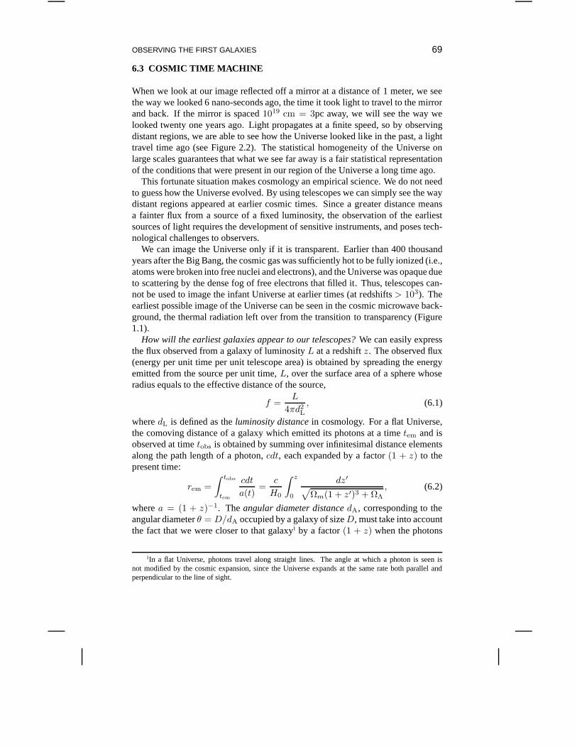
OBSERVING THE FIRST GALAXIES 69
6.3 COSMIC TIME MACHINE
When we look at our image reflected off a mirror at a distance of1 meter, we seethe way we looked 6 nano-seconds ago, the time it took light totravel to the mirrorand back. If the mirror is spaced1019 cm = 3pc away, we will see the way welooked twenty one years ago. Light propagates at a finite speed, so by observingdistant regions, we are able to see how the Universe looked like in the past, a lighttravel time ago (see Figure 2.2). The statistical homogeneity of the Universe onlarge scales guarantees that what we see far away is a fair statistical representationof the conditions that were present in our region of the Universe a long time ago.
This fortunate situation makes cosmology an empirical science. We do not needto guess how the Universe evolved. By using telescopes we cansimply see the waydistant regions appeared at earlier cosmic times. Since a greater distance meansa fainter flux from a source of a fixed luminosity, the observation of the earliestsources of light requires the development of sensitive instruments, and poses tech-nological challenges to observers.
We can image the Universe only if it is transparent. Earlier than 400 thousandyears after the Big Bang, the cosmic gas was sufficiently hot to be fully ionized (i.e.,atoms were broken into free nuclei and electrons), and the Universe was opaque dueto scattering by the dense fog of free electrons that filled it. Thus, telescopes can-not be used to image the infant Universe at earlier times (at redshifts> 103). Theearliest possible image of the Universe can be seen in the cosmic microwave back-ground, the thermal radiation left over from the transitionto transparency (Figure1.1).
How will the earliest galaxies appear to our telescopes?We can easily expressthe flux observed from a galaxy of luminosityL at a redshiftz. The observed flux(energy per unit time per unit telescope area) is obtained byspreading the energyemitted from the source per unit time,L, over the surface area of a sphere whoseradius equals to the effective distance of the source,
f =L
4πd2L
, (6.1)
wheredL is defined as theluminosity distancein cosmology. For a flat Universe,the comoving distance of a galaxy which emitted its photons at a timetem and isobserved at timetobs is obtained by summing over infinitesimal distance elementsalong the path length of a photon,cdt, each expanded by a factor(1 + z) to thepresent time:
rem =
∫ tobs
tem
cdt
a(t)=
c
H0
∫ z
0
dz′√
Ωm(1 + z′)3 + ΩΛ
, (6.2)
wherea = (1 + z)−1. Theangular diameter distancedA, corresponding to theangular diameterθ = D/dA occupied by a galaxy of sizeD, must take into accountthe fact that we were closer to that galaxyi by a factor(1 + z) when the photons
i In a flat Universe, photons travel along straight lines. The angle at which a photon is seen isnot modified by the cosmic expansion, since the Universe expands at the same rate both parallel andperpendicular to the line of sight.
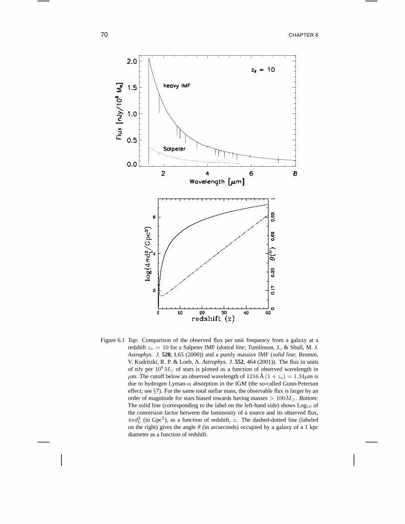
70 CHAPTER 6
Figure 6.1 Top: Comparison of the observed flux per unit frequency from a galaxy at aredshiftzs = 10 for a Salpeter IMF (dotted line; Tumlinson, J., & Shull, M. J.Astrophys. J.528, L65 (2000)) and a purely massive IMF (solid line; Bromm,V. Kudritzki, R. P. & Loeb, A.Astrophys. J.552, 464 (2001)). The flux in unitsof nJy per106M⊙ of stars is plotted as a function of observed wavelength inµm. The cutoff below an observed wavelength of1216 A (1 + zs) = 1.34µm isdue to hydrogen Lyman-α absorption in the IGM (the so-called Gunn-Petersoneffect; see§7). For the same total stellar mass, the observable flux is larger by anorder of magnitude for stars biased towards having masses> 100M⊙. Bottom:The solid line (corresponding to the label on the left-hand side) shows Log10 ofthe conversion factor between the luminosity of a source andits observed flux,4πd2
L (in Gpc2), as a function of redshift,z. The dashed-dotted line (labeledon the right) gives the angleθ (in arcseconds) occupied by a galaxy of a 1 kpcdiameter as a function of redshift.
OBSERVING THE FIRST GALAXIES 71
started their journey at a redshiftz, so it is simply given bydA = rem/(1+ z). Butto finddL we must take account of additional redshift factors.
If a galaxy has an intrinsic luminosityL, then it would emit an energyLdtemover a time intervaldtem. This energy is redshifted by a factor of(1 + z) and isobserved over a longer time intervaldtobs = dtem(1 + z) after being spread over asphere of surface area4πr2
em. Thus, the observed flux would be
f =Ldtem/(1 + z)
4πr2emdtobs
=L
4πr2em(1 + z)2
, (6.3)
implying thatii
dL = rem(1 + z) = dA(1 + z)2. (6.4)
The area dilution factor4πd2L is plotted as a function of redshift in the bottom panel
of Figure 6.1. If the observed flux is only measured over a narrow band of frequen-cies, one needs to take account of the additional conversionfactor of (1 + z) =(dνem/dνobs) between the emitted frequency intervaldνem and its observed valuedνobs. This yields the relation(df/dνobs) = (1+z)×(dL/dνem)/(4πd2
L). The toppanel of Figure 6.1 compares the predicted flux per unit frequencyiii from a galaxyat a redshiftzs = 10 for a Salpeter IMF and for massive (> 100M⊙) Population IIIstars, in units of nJy per106M⊙ in stars (where 1 nJy= 10−32 erg cm−2 s−1 Hz−1).The observed flux is an order of magnitude larger in the Population III case. Thestrong UV emission by massive stars is likely to produce bright recombination lines(such as Lyman-α and He II 1640A) from the interstellar medium surroundingthese stars.
Theoretically, the expected number of early galaxies of different fluxes per unitarea on the sky can be calculated by dressing up the dark matter halos in Figure 3.2with stars of some prescribed mass distribution and formation history, then findingthe corresponding abundance of galaxies of different luminosities as a function ofredshift.62 There are many uncertain parameters in this approach (such as f⋆, fesc,the stellar mass function, the star formation time, the metallicity, and feedback), soone is tempted to calibrate these parameters by observing the sky.63
6.4 THE HUBBLE DEEP FIELD AND ITS FOLLOW-UPS
In 1995, Bob Williams, then Director of the Space Telescope Science Institute, in-vited leading astronomers to advise him where to point the Hubble Space Telescope(HST) during the discretionary time he received as a Director, which amounted to atotal of up to 10% of HST’s observing time.iv Each of the invited experts presenteda detailed plan for using HST’s time in sensible, but complex, observing programsaddressing their personal research interests. After much of the day had passed, it
ii A simple analytic fitting formula fordL(z) was derived by Pen, U.-L.Astrophys. J. Suppl.120,49 (1999); http://arxiv.org/pdf/astro-ph/9904172v1 .
iii The observed flux per unit frequency can be translated to an equivalent AB magnitude using therelation,AB ≡ −2.5 log10[(df/dνobs)/erg s−1 cm−2 Hz−1] − 48.6.
ivTurner, E. private communication (2009).
72 CHAPTER 6
became obvious that no consensus would be reached. “What shall we do?” askedone of the participants. Out of desperation, another participant suggested, “Whydon’t we point the telescope towards a fixed non-special direction and burn a holein the sky as deep as we can go?” – just like checking how fast your new car cango. This simple compromise won the day since there was no realbasis for choos-ing among the more specialized suggestions. As it turned out, this “hole burning”choice was one of the most influential uses of HST as it produced the deepest imagewe have so far of the cosmos.
The Hubble Deep Field (HDF) covered an area of 5.3 squared arcminutes andwas observed over 10 days (see Figure 6.2). One of its pioneering findings was thediscovery of large numbers of high-redshift galaxies at a time when only a smallnumber of galaxies atz > 1 were known.v The HDF contained many red galaxieswith some reaching a redshift as high as6, or even higher.64 The wealth of galaxiesdiscovered at different stages of their evolution allowed astronomers to estimate thevariation in the global rate of star formation per comoving volume over the lifetimeof the universe.
Subsequent incarnations of this successful approach included the HDF-Southand the Great Observatories Origins Deep Survey (GOODS). A section of GOODS,occupying a tenth of the diameter of the full moon (equivalent to 11 square arcmin-utes), was then observed for a total exposure time of a million seconds to create theHubble Ultra Deep Field (HUDF), the most sensitive deep fieldimage in visiblelight to date.vi Red galaxies were identified in the HUDF image up to a redshiftofz ∼ 7, and possibly even higher, showing that the typical UV luminosity of galax-ies declines with redshift atz > 4.65 The redshifts of galaxies are inferred eitherthrough a search for a Lyman-α emission line (identifying so-called “Lyman-αgalaxies”),66 or through a search for a spectral break associated with the absorp-tion of intervening hydrogen (so-called “Lyman-break galaxies”).67 For very faintsources, redshifts are only identified crudely based on the spectral trough producedby hydrogen absorption in the host galaxy and the IGM (see§7).
The abundance of Lyman-α galaxies shows a strong decline betweenz = 5.7 andz = 7, as expected from a correspondingly rapid increase in the neutral fractionof the IGM (which would scatter the Lyman-α line photons and make the lineemission from these galaxies undetectable),68 but this interpretation is not unique.
The mass budget of stars atz ∼ 5–6 has been inferred from complementaryinfrared observation with the Spitzer Space Telescope (seeFig. 6.3). The mean ageof the stars in individual galaxies implies that they had formed atz ∼ 10 and couldhave produced sufficient photons to reionize the IGM.
Another approach adopted by observers benefits from magnifying devices pro-vided for free by nature, so-called “gravitational lenses.” Rich clusters of galaxieshave such a large concentration of mass that their gravity bends the light-rays fromany source behind them and magnifies its image. This allows observers to probefainter galaxies at higher redshifts than ever probed before. The redshift record
vJust prior to the HDF, an important paper about high-redshift galaxies was declined for publicationbecause the referee pointed out the “well-known fact” that there are no galaxies beyond a redshift of 1.
vi In order for galaxy surveys to be statistically reliable, they need to cover large areas of the sky.Counts of galaxies in small fields of view suffer from a large cosmic variance owing to galaxy clustering.
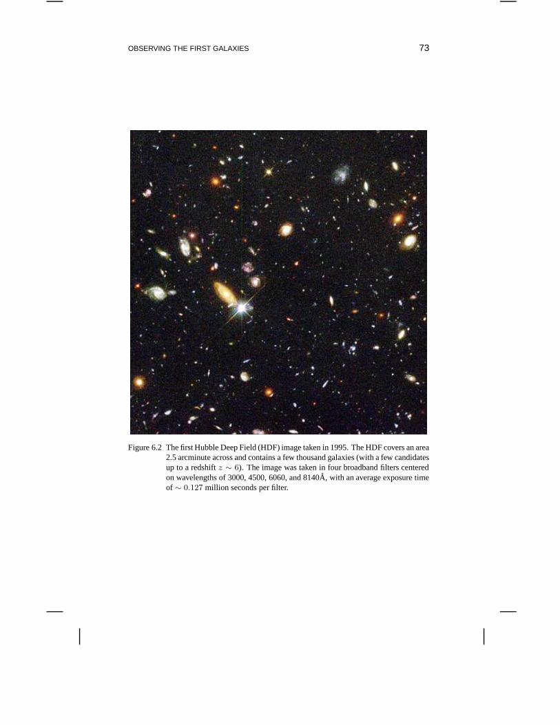
OBSERVING THE FIRST GALAXIES 73
Figure 6.2 The first Hubble Deep Field (HDF) image taken in 1995. The HDF covers an area2.5 arcminute across and contains a few thousand galaxies (with a few candidatesup to a redshiftz ∼ 6). The image was taken in four broadband filters centeredon wavelengths of 3000, 4500, 6060, and 8140A, with an average exposure timeof ∼ 0.127 million seconds per filter.
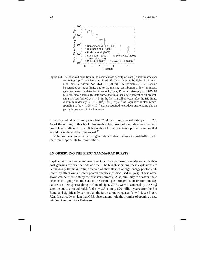
74 CHAPTER 6
0 1 2 3 4 5 6Redshift
105
106
107
108
109
Ste
llar
Mas
s D
ensi
ty /
Msu
nMpc
-3
Shankar et al. (2006)Cole et al. (2001)
Brinchmann & Ellis (2000)Dickinson et al. (2003)Rudnick et al. (2003)Stark et al. (2007)Yan et al. (2006)
Eyles et al. (2007)
Figure 6.3 The observed evolution in the cosmic mass densityof stars (in solar masses percomoving Mpc3) as a function of redshift [data compiled by Eyles, L. P., et al.Mon. Not. R. Astron. Soc.374, 910 (2007)]. The estimates atz > 5 shouldbe regarded as lower limits due to the missing contribution of low-luminositygalaxies below the detection threshold [Stark, D., et al.Astrophys. J.659, 84(2007)]. Nevertheless, the data shows that less than a few percent of all present-day stars had formed atz > 5, in the first 1.2 billion years after the Big Bang.A minimum density∼ 1.7 × 10⁶f−1
esc M⊙ Mpc−3 of Population II stars (corre-sponding toΩ⋆ ∼ 1.25 × 10⁻⁵f−1
esc ) is required to produce one ionizing photonper hydrogen atom in the Universe.
from this method is currently associated69 with a strongly lensed galaxy atz = 7.6.As of the writing of this book, this method has provided candidate galaxies withpossible redshifts up toz ∼ 10, but without further spectroscopic confirmation thatwould make these detections robust.70
So far, we have not seen the first generation of dwarf galaxiesat redshiftsz > 10that were responsible for reionization.
6.5 OBSERVING THE FIRST GAMMA-RAY BURSTS
Explosions of individual massive stars (such as supernovae) can also outshine theirhost galaxies for brief periods of time. The brightest amongthese explosions areGamma-Ray Bursts (GRBs), observed as short flashes of high-energy photons fol-lowed by afterglows at lower photon energies (as discussed in §4.4). These after-glows can be used to study the first stars directly. Also, similarly to quasars, thesebeacons of light probe the state of the cosmic gas through itsabsorption line sig-natures on their spectra along the line of sight. GRBs were discovered by theSwiftsatellite out to a record redshift ofz = 8.3, merely 620 million years after the BigBang, and significantly earlier than the farthest known quasar (z = 6.4, see Figure7.2). It is already evident that GRB observations hold the promise of opening a newwindow into the infant Universe.
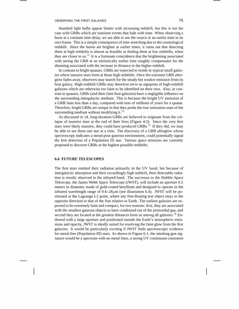
OBSERVING THE FIRST GALAXIES 75
Standard light bulbs appear fainter with increasing redshift, but this is not thecase with GRBs which are transient events that fade with time. When observing aburst at a constant time delay, we are able to see the source atan earlier time in itsown frame. This is a simple consequence of time stretching due to the cosmologicalredshift. Since the bursts are brighter at earlier times, itturns out that detectingthem at high redshifts is almost as feasible as finding them atlow redshifts, whenthey are closer to us.71 It is a fortunate coincidence that the brightening associatedwith seeing the GRB at an intrinsically earlier time roughlycompensates for thedimming associated with the increase in distance to the higher redshift.
In contrast to bright quasars, GRBs are expected to reside intypical small galax-ies where massive stars form at those high redshifts. Once the transient GRB after-glow fades away, observers may search for the steady but weaker emission from itshost galaxy. High-redshift GRBs may therefore serve as signposts of high-redshiftgalaxies which are otherwise too faint to be identified on their own. Also, in con-trast to quasars, GRBs (and their faint host galaxies) have anegligible influence onthe surrounding intergalactic medium. This is because the bright UV emission ofa GRB lasts less than a day, compared with tens of millions of years for a quasar.Therefore, bright GRBs are unique in that they probe the trueionization state of thesurrounding medium without modifying it.72
As discussed in§4, long-duration GRBs are believed to originate from the col-lapse of massive stars at the end of their lives (Figure 4.5).Since the very firststars were likely massive, they could have produced GRBs.73 If they did, we maybe able to see them one star at a time. The discovery of a GRB afterglow whosespectroscopy indicates a metal-poor gaseous environment,could potentially signalthe first detection of a Population III star. Various space missions are currentlyproposed to discover GRBs at the highest possible redshifts.
6.6 FUTURE TELESCOPES
The first stars emitted their radiation primarily in the UV band, but because ofintergalactic absorption and their exceedingly high redshift, their detectable radia-tion is mostly observed in the infrared band. The successor to the Hubble SpaceTelescope, the James Webb Space Telescope (JWST), will include an aperture 6.5meters in diameter, made of gold-coated beryllium and designed to operate in theinfrared wavelength range of 0.6–28µm (see illustration 6.4). JWST will be po-sitioned at the Lagrange L2 point, where any free-floating test object stays in theopposite direction to that of the Sun relative to Earth. The earliest galaxies are ex-pected to be extremely faint and compact, for two reasons: first, they are associatedwith the smallest gaseous objects to have condensed out of the primordial gas, andsecond they are located at the greatest distances from us among all galaxies.74 En-dowed with a large aperture and positioned outside the Earth’s atmospheric emis-sions and opacity, JWST is ideally suited for resolving the faint glow from the firstgalaxies. It would be particularly exciting if JWST finds spectroscopic evidencefor metal-free (Population III) stars. As shown in Figure 6.1, the smoking gun sig-nature would be a spectrum with no metal lines, a strong UV continuum consistent
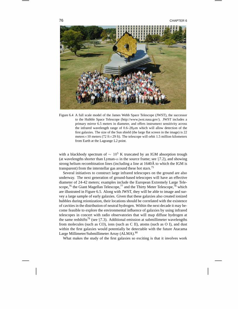
76 CHAPTER 6
Figure 6.4 A full scale model of the James Webb Space Telescope (JWST), the successorto the Hubble Space Telescope (http://www.jwst.nasa.gov/). JWST includes aprimary mirror 6.5 meters in diameter, and offers instrument sensitivity acrossthe infrared wavelength range of 0.6–28µm which will allow detection of thefirst galaxies. The size of the Sun shield (the large flat screen in the image) is 22meters×10 meters (72 ft×29 ft). The telescope will orbit 1.5 million kilometersfrom Earth at the Lagrange L2 point.
with a blackbody spectrum of∼ 105 K truncated by an IGM absorption trough(at wavelengths shorter than Lyman-α in the source frame; see§7.2), and showingstrong helium recombination lines (including a line at 1640A to which the IGM istransparent) from the interstellar gas around these hot stars.75
Several initiatives to construct large infrared telescopes on the ground are alsounderway. The next generation of ground-based telescopes will have an effectivediameter of 24-42 meters; examples include the European Extremely Large Tele-scope,76 the Giant Magellan Telescope,77 and the Thirty Meter Telescope,78 whichare illustrated in Figure 6.5. Along with JWST, they will be able to image and sur-vey a large sample of early galaxies. Given that these galaxies also created ionizedbubbles during reionization, their locations should be correlated with the existenceof cavities in the distribution of neutral hydrogen. Withinthe next decade it may be-come feasible to explore the environmental influence of galaxies by using infraredtelescopes in concert with radio observatories that will map diffuse hydrogen atthe same redshifts79 (see§7.3). Additional emission at submillimeter wavelengthsfrom molecules (such as CO), ions (such as C II), atoms (such as O I), and dustwithin the first galaxies would potentially be detectable with the future AtacamaLarge Millimeter/Submillimeter Array (ALMA).80
What makes the study of the first galaxies so exciting is that it involves work
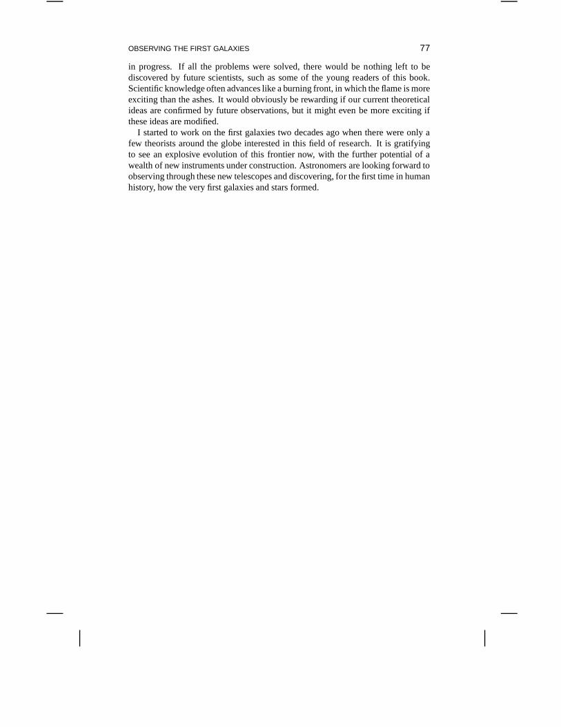
OBSERVING THE FIRST GALAXIES 77
in progress. If all the problems were solved, there would be nothing left to bediscovered by future scientists, such as some of the young readers of this book.Scientific knowledge often advances like a burning front, inwhich the flame is moreexciting than the ashes. It would obviously be rewarding if our current theoreticalideas are confirmed by future observations, but it might evenbe more exciting ifthese ideas are modified.
I started to work on the first galaxies two decades ago when there were only afew theorists around the globe interested in this field of research. It is gratifyingto see an explosive evolution of this frontier now, with the further potential of awealth of new instruments under construction. Astronomersare looking forward toobserving through these new telescopes and discovering, for the first time in humanhistory, how the very first galaxies and stars formed.
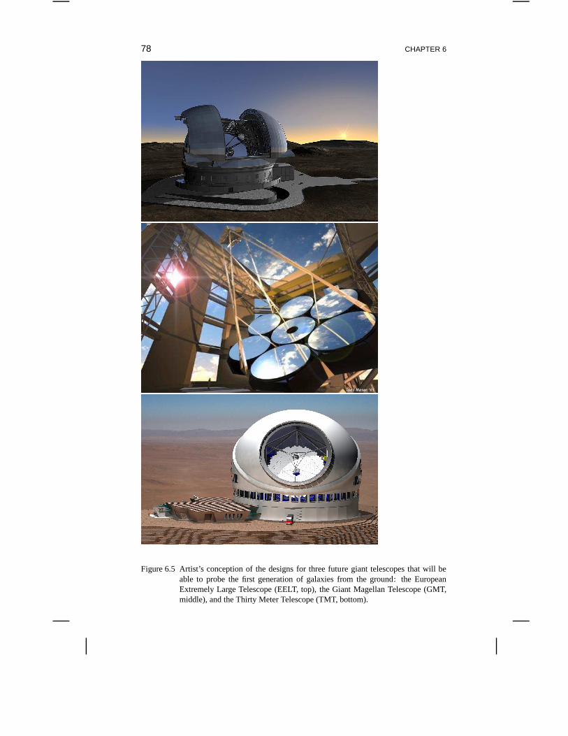
78 CHAPTER 6
Figure 6.5 Artist’s conception of the designs for three future giant telescopes that will beable to probe the first generation of galaxies from the ground: the EuropeanExtremely Large Telescope (EELT, top), the Giant Magellan Telescope (GMT,middle), and the Thirty Meter Telescope (TMT, bottom).
Chapter Seven
Imaging the Diffuse Fog of Cosmic Hydrogen
7.1 HYDROGEN
Hydrogen is the most abundant element in the Universe. It is also the simplest atompossible, containing a proton and an electron held togetherby their mutual electricattraction. Because of its simplicity, the detailed understanding of the hydrogenatom structure played an important role in the development of quantum mechanics.
Since the lifetime of energy levels with principal quantum numbern greaterthan 1 is far shorter than the typical time it takes to excite them in the rarefiedenvironments of the Universe, hydrogen is commonly found tobe in its groundstate (lowest energy level) withn = 1. This implies that the transitions we shouldfocus on are those that involve then = 1 state. Below we describe two suchtransitions, depicted in Figure 7.1.
7.2 THE LYMAN- α LINE
The most widely discussed transition of hydrogen in cosmology is the Lyman-αspectral line, which was discovered experimentally in 1905by Harvard physicistTheodore Lyman. This line has been traditionally used to probe the ionization stateof the IGM in the spectra of quasars, galaxies, and gamma-raybursts. Back in1965, Peter Scheuer81 and, independently, Jim Gunn & Bruce Peterson82 realizedthat the cross-section for Lyman-α absorption is so large that the IGM should beopaque to iti even if its neutral (non-ionized) fraction is as small as∼ 10−5. Thelack of complete absorption for quasars at redshiftsz < 6.4 is now interpreted asevidence that the diffuse IGM was fully ionized within less than a billion years afterthe Big Bang. Quasar spectra do show evidence for a so-called“forest” of Lyman-αabsorption features, which originate from slight enhancements in the tiny fractionof hydrogen within overdense regions of the cosmic web. The Lyman-α foresthas so far been observed in the spectrum of widely separated “skewers” pointingtowards individual quasars. Since the cosmic web provides ameasure of the powerspectrumP (k), there are plans to observe a dense array of skewers associated witha large number of quasars and map the related large-scale structure it delineates inthree dimensions.
If a source were to be observed before or during the epoch of reionization, when
iThe optical depth for Lyman-α absorption out to a source at a redshiftzs by an IGM with anatomic hydrogen fractionxHI is τ ≈ 7 × 10⁵xHI[(1 + zs)/10]3/2 .
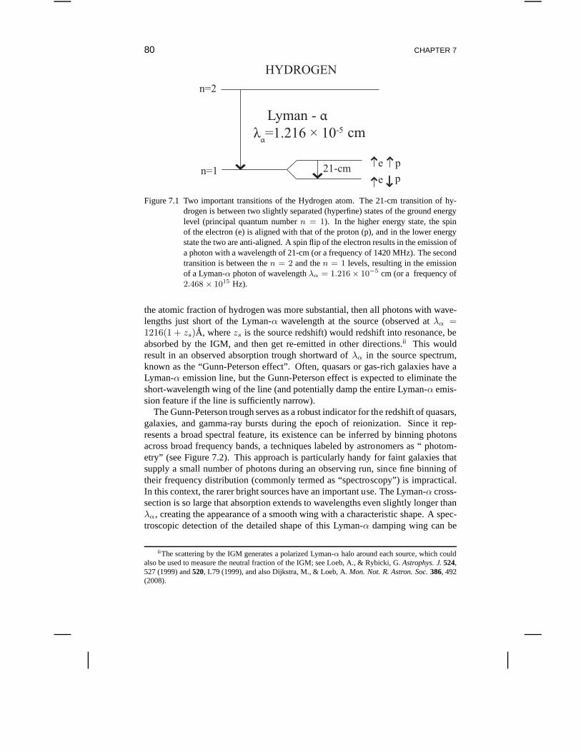
80 CHAPTER 7
Lyman - α λα=1.216 × 10⁻⁵ cm
n=2
n=1
HYDROGEN
21-cme p
e p
Figure 7.1 Two important transitions of the Hydrogen atom. The 21-cm transition of hy-drogen is between two slightly separated (hyperfine) statesof the ground energylevel (principal quantum numbern = 1). In the higher energy state, the spinof the electron (e) is aligned with that of the proton (p), andin the lower energystate the two are anti-aligned. A spin flip of the electron results in the emission ofa photon with a wavelength of 21-cm (or a frequency of 1420 MHz). The secondtransition is between then = 2 and then = 1 levels, resulting in the emissionof a Lyman-α photon of wavelengthλα = 1.216 × 10⁻⁵ cm (or a frequency of2.468 × 1015 Hz).
the atomic fraction of hydrogen was more substantial, then all photons with wave-lengths just short of the Lyman-α wavelength at the source (observed atλα =1216(1 + zs)A, wherezs is the source redshift) would redshift into resonance, beabsorbed by the IGM, and then get re-emitted in other directions.ii This wouldresult in an observed absorption trough shortward ofλα in the source spectrum,known as the “Gunn-Peterson effect”. Often, quasars or gas-rich galaxies have aLyman-α emission line, but the Gunn-Peterson effect is expected to eliminate theshort-wavelength wing of the line (and potentially damp theentire Lyman-α emis-sion feature if the line is sufficiently narrow).
The Gunn-Peterson trough serves as a robust indicator for the redshift of quasars,galaxies, and gamma-ray bursts during the epoch of reionization. Since it rep-resents a broad spectral feature, its existence can be inferred by binning photonsacross broad frequency bands, a techniques labeled by astronomers as “ photom-etry” (see Figure 7.2). This approach is particularly handyfor faint galaxies thatsupply a small number of photons during an observing run, since fine binning oftheir frequency distribution (commonly termed as “spectroscopy”) is impractical.In this context, the rarer bright sources have an important use. The Lyman-α cross-section is so large that absorption extends to wavelengths even slightly longer thanλα, creating the appearance of a smooth wing with a characteristic shape. A spec-troscopic detection of the detailed shape of this Lyman-α damping wing can be
ii The scattering by the IGM generates a polarized Lyman-α halo around each source, which couldalso be used to measure the neutral fraction of the IGM; see Loeb, A., & Rybicki, G.Astrophys. J.524,527 (1999) and520, L79 (1999), and also Dijkstra, M., & Loeb, A.Mon. Not. R. Astron. Soc.386, 492(2008).
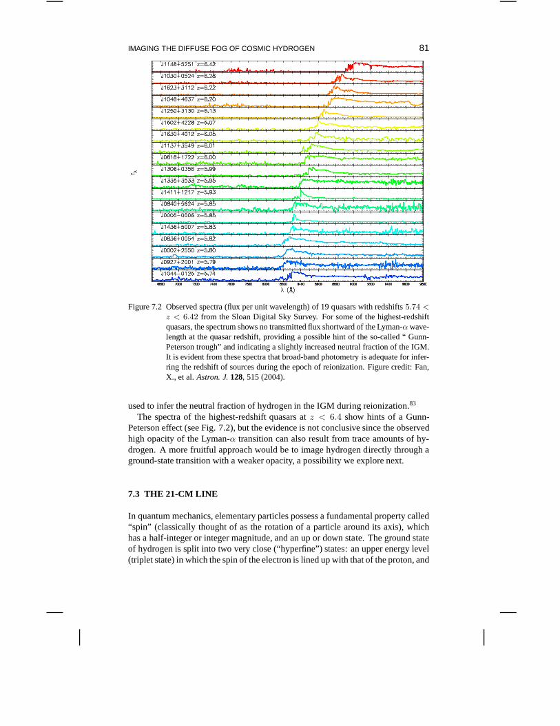
IMAGING THE DIFFUSE FOG OF COSMIC HYDROGEN 81
Figure 7.2 Observed spectra (flux per unit wavelength) of 19 quasars with redshifts5.74 <z < 6.42 from the Sloan Digital Sky Survey. For some of the highest-redshiftquasars, the spectrum shows no transmitted flux shortward ofthe Lyman-α wave-length at the quasar redshift, providing a possible hint of the so-called “ Gunn-Peterson trough” and indicating a slightly increased neutral fraction of the IGM.It is evident from these spectra that broad-band photometryis adequate for infer-ring the redshift of sources during the epoch of reionization. Figure credit: Fan,X., et al.Astron. J.128, 515 (2004).
used to infer the neutral fraction of hydrogen in the IGM during reionization.83
The spectra of the highest-redshift quasars atz < 6.4 show hints of a Gunn-Peterson effect (see Fig. 7.2), but the evidence is not conclusive since the observedhigh opacity of the Lyman-α transition can also result from trace amounts of hy-drogen. A more fruitful approach would be to image hydrogen directly through aground-state transition with a weaker opacity, a possibility we explore next.
7.3 THE 21-CM LINE
In quantum mechanics, elementary particles possess a fundamental property called“spin” (classically thought of as the rotation of a particlearound its axis), whichhas a half-integer or integer magnitude, and an up or down state. The ground stateof hydrogen is split into two very close (“hyperfine”) states: an upper energy level(triplet state) in which the spin of the electron is lined up with that of the proton, and
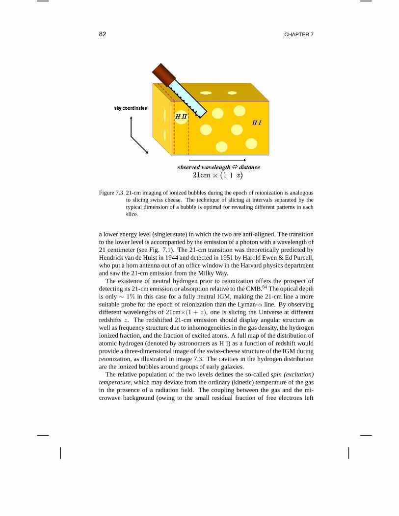
82 CHAPTER 7
Figure 7.3 21-cm imaging of ionized bubbles during the epochof reionization is analogousto slicing swiss cheese. The technique of slicing at intervals separated by thetypical dimension of a bubble is optimal for revealing different patterns in eachslice.
a lower energy level (singlet state) in which the two are anti-aligned. The transitionto the lower level is accompanied by the emission of a photon with a wavelength of21 centimeter (see Fig. 7.1). The 21-cm transition was theoretically predicted byHendrick van de Hulst in 1944 and detected in 1951 by Harold Ewen & Ed Purcell,who put a horn antenna out of an office window in the Harvard physics departmentand saw the 21-cm emission from the Milky Way.
The existence of neutral hydrogen prior to reionization offers the prospect ofdetecting its 21-cm emission or absorption relative to the CMB.84 The optical depthis only∼ 1% in this case for a fully neutral IGM, making the 21-cm line a moresuitable probe for the epoch of reionization than the Lyman-α line. By observingdifferent wavelengths of 21cm×(1 + z), one is slicing the Universe at differentredshiftsz. The redshifted 21-cm emission should display angular structure aswell as frequency structure due to inhomogeneities in the gas density, the hydrogenionized fraction, and the fraction of excited atoms. A full map of the distribution ofatomic hydrogen (denoted by astronomers as H I) as a functionof redshift wouldprovide a three-dimensional image of the swiss-cheese structure of the IGM duringreionization, as illustrated in image 7.3. The cavities in the hydrogen distributionare the ionized bubbles around groups of early galaxies.
The relative population of the two levels defines the so-calledspin (excitation)temperature, which may deviate from the ordinary (kinetic) temperatureof the gasin the presence of a radiation field. The coupling between thegas and the mi-crowave background (owing to the small residual fraction offree electrons left
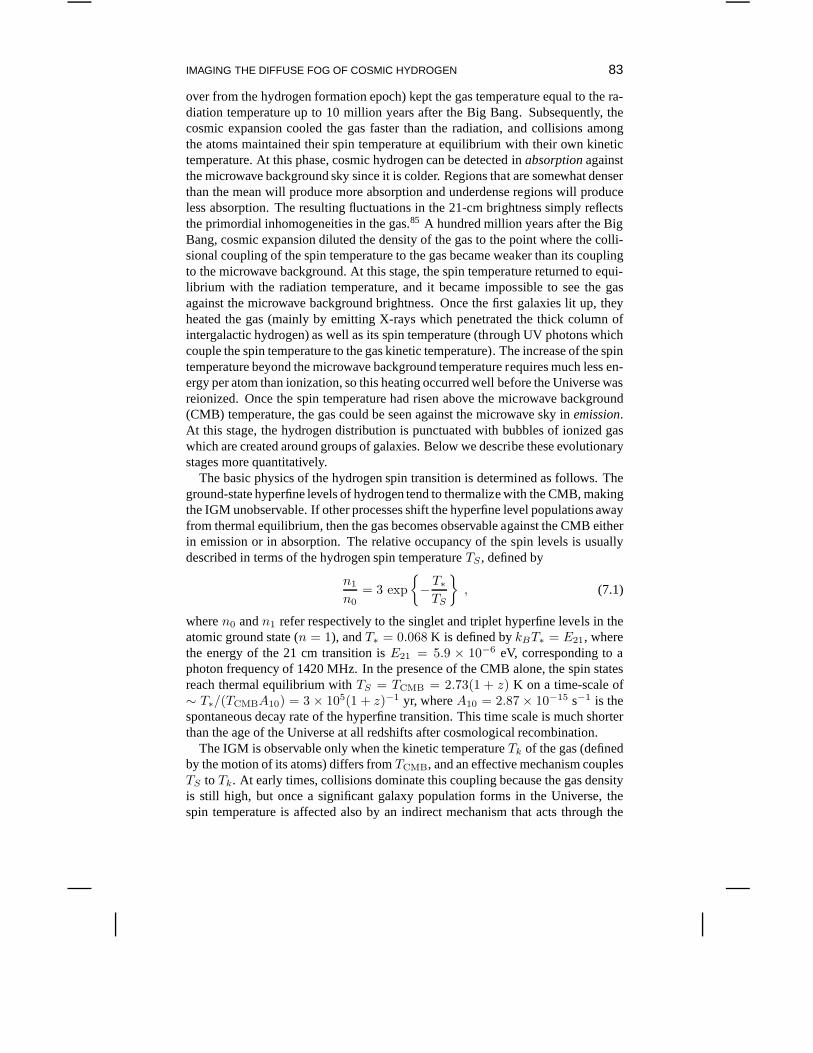
IMAGING THE DIFFUSE FOG OF COSMIC HYDROGEN 83
over from the hydrogen formation epoch) kept the gas temperature equal to the ra-diation temperature up to 10 million years after the Big Bang. Subsequently, thecosmic expansion cooled the gas faster than the radiation, and collisions amongthe atoms maintained their spin temperature at equilibriumwith their own kinetictemperature. At this phase, cosmic hydrogen can be detectedin absorptionagainstthe microwave background sky since it is colder. Regions that are somewhat denserthan the mean will produce more absorption and underdense regions will produceless absorption. The resulting fluctuations in the 21-cm brightness simply reflectsthe primordial inhomogeneities in the gas.85 A hundred million years after the BigBang, cosmic expansion diluted the density of the gas to the point where the colli-sional coupling of the spin temperature to the gas became weaker than its couplingto the microwave background. At this stage, the spin temperature returned to equi-librium with the radiation temperature, and it became impossible to see the gasagainst the microwave background brightness. Once the firstgalaxies lit up, theyheated the gas (mainly by emitting X-rays which penetrated the thick column ofintergalactic hydrogen) as well as its spin temperature (through UV photons whichcouple the spin temperature to the gas kinetic temperature). The increase of the spintemperature beyond the microwave background temperature requires much less en-ergy per atom than ionization, so this heating occurred wellbefore the Universe wasreionized. Once the spin temperature had risen above the microwave background(CMB) temperature, the gas could be seen against the microwave sky inemission.At this stage, the hydrogen distribution is punctuated withbubbles of ionized gaswhich are created around groups of galaxies. Below we describe these evolutionarystages more quantitatively.
The basic physics of the hydrogen spin transition is determined as follows. Theground-state hyperfine levels of hydrogen tend to thermalize with the CMB, makingthe IGM unobservable. If other processes shift the hyperfinelevel populations awayfrom thermal equilibrium, then the gas becomes observable against the CMB eitherin emission or in absorption. The relative occupancy of the spin levels is usuallydescribed in terms of the hydrogen spin temperatureTS , defined by
n1
n0= 3 exp
−T∗
TS
, (7.1)
wheren0 andn1 refer respectively to the singlet and triplet hyperfine levels in theatomic ground state (n = 1), andT∗ = 0.068 K is defined bykBT∗ = E21, wherethe energy of the 21 cm transition isE21 = 5.9 × 10⁻⁶ eV, corresponding to aphoton frequency of 1420 MHz. In the presence of the CMB alone, the spin statesreach thermal equilibrium withTS = TCMB = 2.73(1 + z) K on a time-scale of∼ T∗/(TCMBA10) = 3 × 10⁵(1 + z)−1 yr, whereA10 = 2.87 × 10⁻¹⁵ s−1 is thespontaneous decay rate of the hyperfine transition. This time scale is much shorterthan the age of the Universe at all redshifts after cosmological recombination.
The IGM is observable only when the kinetic temperatureTk of the gas (definedby the motion of its atoms) differs fromTCMB, and an effective mechanism couplesTS to Tk. At early times, collisions dominate this coupling becausethe gas densityis still high, but once a significant galaxy population formsin the Universe, thespin temperature is affected also by an indirect mechanism that acts through the
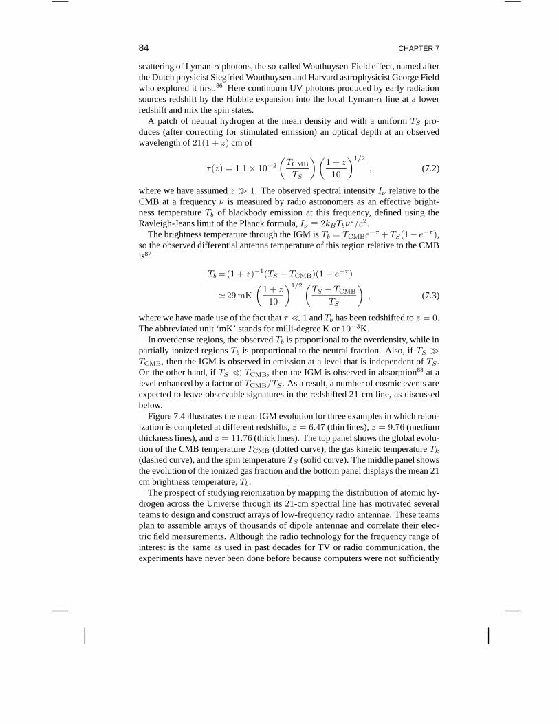
84 CHAPTER 7
scattering of Lyman-α photons, the so-called Wouthuysen-Field effect, named afterthe Dutch physicist Siegfried Wouthuysen and Harvard astrophysicist George Fieldwho explored it first.86 Here continuum UV photons produced by early radiationsources redshift by the Hubble expansion into the local Lyman-α line at a lowerredshift and mix the spin states.
A patch of neutral hydrogen at the mean density and with a uniform TS pro-duces (after correcting for stimulated emission) an optical depth at an observedwavelength of21(1 + z) cm of
τ(z) = 1.1 × 10⁻²
(
TCMB
TS
) (
1 + z
10
)1/2
, (7.2)
where we have assumedz ≫ 1. The observed spectral intensityIν relative to theCMB at a frequencyν is measured by radio astronomers as an effective bright-ness temperatureTb of blackbody emission at this frequency, defined using theRayleigh-Jeans limit of the Planck formula,Iν ≡ 2kBTbν
2/c2.The brightness temperature through the IGM isTb = TCMBe−τ + TS(1− e−τ ),
so the observed differential antenna temperature of this region relative to the CMBis87
Tb =(1 + z)−1(TS − TCMB)(1 − e−τ )
≃ 29 mK
(
1 + z
10
)1/2 (
TS − TCMB
TS
)
, (7.3)
where we have made use of the fact thatτ ≪ 1 andTb has been redshifted toz = 0.The abbreviated unit ‘mK’ stands for milli-degree K or10−3K.
In overdense regions, the observedTb is proportional to the overdensity, while inpartially ionized regionsTb is proportional to the neutral fraction. Also, ifTS ≫TCMB, then the IGM is observed in emission at a level that is independent ofTS.On the other hand, ifTS ≪ TCMB, then the IGM is observed in absorption88 at alevel enhanced by a factor ofTCMB/TS. As a result, a number of cosmic events areexpected to leave observable signatures in the redshifted 21-cm line, as discussedbelow.
Figure 7.4 illustrates the mean IGM evolution for three examples in which reion-ization is completed at different redshifts,z = 6.47 (thin lines),z = 9.76 (mediumthickness lines), andz = 11.76 (thick lines). The top panel shows the global evolu-tion of the CMB temperatureTCMB (dotted curve), the gas kinetic temperatureTk
(dashed curve), and the spin temperatureTS (solid curve). The middle panel showsthe evolution of the ionized gas fraction and the bottom panel displays the mean 21cm brightness temperature,Tb.
The prospect of studying reionization by mapping the distribution of atomic hy-drogen across the Universe through its 21-cm spectral line has motivated severalteams to design and construct arrays of low-frequency radioantennae. These teamsplan to assemble arrays of thousands of dipole antennae and correlate their elec-tric field measurements. Although the radio technology for the frequency range ofinterest is the same as used in past decades for TV or radio communication, theexperiments have never been done before because computers were not sufficiently
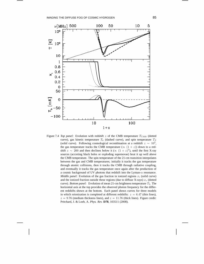
IMAGING THE DIFFUSE FOG OF COSMIC HYDROGEN 85
Figure 7.4 Top panel: Evolution with redshiftz of the CMB temperatureTCMB (dottedcurve), gas kinetic temperatureTk (dashed curve), and spin temperatureTS
(solid curve). Following cosmological recombination at a redshift z ∼ 103,the gas temperature tracks the CMB temperature (∝ (1 + z)) down to a red-shift z ∼ 200 and then declines below it (∝ (1 + z)2), until the first X-raysources (accreting black holes or exploding supernovae) heat it up well abovethe CMB temperature. The spin temperature of the 21-cm transition interpolatesbetween the gas and CMB temperatures; initially it tracks the gas temperaturethrough atomic collisions, then it tracks the CMB through radiative coupling,and eventually it tracks the gas temperature once again after the production ofa cosmic background of UV photons that redshift into the Lyman-α resonance.Middle panel: Evolution of the gas fraction in ionized regionsxi (solid curve)and the ionized fraction outside these regions (due to diffuse X-rays)xe (dottedcurve).Bottom panel: Evolution of mean 21-cm brightness temperatureTb. Thehorizontal axis at the top provides the observed photon frequency for the differ-ent redshifts shown at the bottom. Each panel shows curves for three modelsin which reionization is completed at different redshifts:z = 6.47 (thin lines),z = 9.76 (medium thickness lines), andz = 11.76 (thick lines). Figure credit:Pritchard, J. & Loeb, A.Phys. Rev.D78, 103511 (2008).
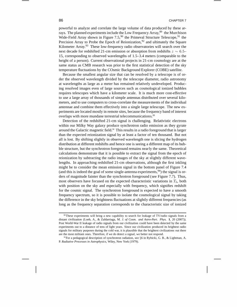
86 CHAPTER 7
powerful to analyze and correlate the large volume of data produced by these ar-rays. The planned experiments include the Low Frequency Array,89 the MurchisonWide-Field Array shown in Figure 7.5,90 the Primeval Structure Telescope,91 thePrecision Array to Probe the Epoch of Reionization,92 and ultimately the SquareKilometer Array.93 These low-frequency radio observatories will search over thenext decade for redshifted 21-cm emission or absorption from redshiftsz ∼ 6.5–15, corresponding to observed wavelengths of 1.5–3.4 meters (comparable to theheight of a person). Current observational projects in 21-cm cosmology are at thesame status as CMB research was prior to the first statisticaldetection of the skytemperature fluctuations by the COsmic Background Explorer(COBE) satellite.
Because the smallest angular size that can be resolved by a telescope is of or-der the observed wavelength divided by the telescope diameter, radio astronomyat wavelengths as large as a meter has remained relatively undeveloped. Produc-ing resolved images even of large sources such as cosmological ionized bubblesrequires telescopes which have a kilometer scale. It is muchmore cost-effectiveto use a large array of thousands of simple antennas distributed over several kilo-meters, and to use computers to cross-correlate the measurements of the individualantennae and combine them effectively into a single large telescope. The new ex-periments are located mostly in remote sites, because the frequency band of interestoverlaps with more mundane terrestrial telecommunications.iii
Detection of the redshifted 21-cm signal is challenging. Relativistic electronswithin our Milky Way galaxy produce synchrotron radio emission as they gyratearound the Galactic magnetic field.iv This results in a radio foreground that is largerthan the expected reionization signal by at least a factor often thousand. But notall is lost. By shifting slightly in observed wavelength oneis slicing the hydrogendistribution at different redshifts and hence one is seeinga different map of its bub-ble structure, but the synchrotron foreground remains nearly the same. Theoreticalcalculations demonstrate that it is possible to extract thesignal from the epoch ofreionization by subtracting the radio images of the sky at slightly different wave-lengths. In approaching redshifted 21-cm observations, although the first inklingmight be to consider the mean emission signal in the bottom panel of Figure 7.4(and this is indeed the goal of some single-antenna experiments,94) the signal is or-ders of magnitude fainter than the synchrotron foreground (see Figure 7.7). Thus,most observers have focused on the expected characteristicvariations inTb, bothwith position on the sky and especially with frequency, which signifies redshiftfor the cosmic signal. The synchrotron foreground is expected to have a smoothfrequency spectrum, so it is possible to isolate the cosmological signal by takingthe difference in the sky brightness fluctuations at slightly different frequencies (aslong as the frequency separation corresponds to the characteristic size of ionized
iii These experiments will bring a new capability to search for leakage of TV/radio signals from adistant civilization (Loeb, A., & Zaldarriaga, M.J. of Cosm. and Astro-Part. Phys.1, 20 (2007)).Post World-War II leakage of radio signals from our civilization could have been detected by the sameexperiments out to a distance of tens of light years. Since our civilization produced its brightest radiosignals for military purposes during the cold war, it is plausible that the brightest civilizations out thereare the most militant ones. Therefore, if we do detect a signal, we better not respond.
ivFor a pedagogical description of synchrotron radiation, see §6 in Rybicki, G. B., & Lightman, A.P.Radiative Processes in Astrophysics, Wiley, New York (1979).
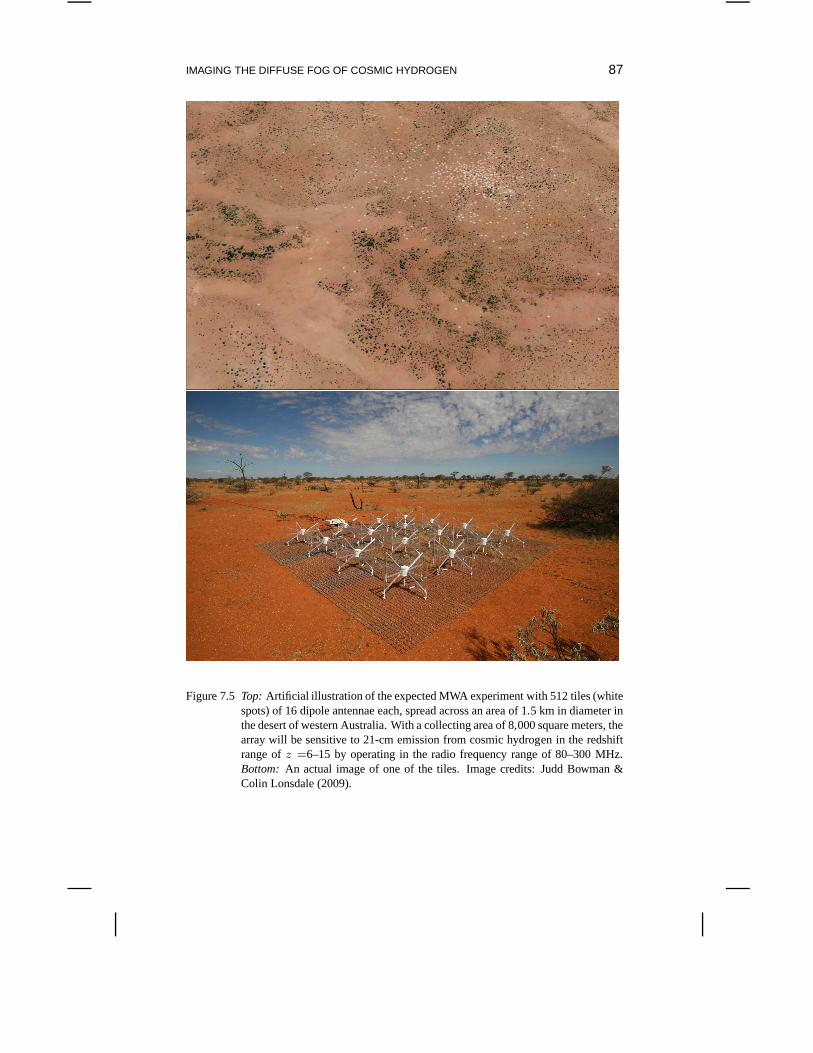
IMAGING THE DIFFUSE FOG OF COSMIC HYDROGEN 87
Figure 7.5 Top: Artificial illustration of the expected MWA experiment with512 tiles (whitespots) of 16 dipole antennae each, spread across an area of 1.5 km in diameter inthe desert of western Australia. With a collecting area of 8,000 square meters, thearray will be sensitive to 21-cm emission from cosmic hydrogen in the redshiftrange ofz =6–15 by operating in the radio frequency range of 80–300 MHz.Bottom: An actual image of one of the tiles. Image credits: Judd Bowman &Colin Lonsdale (2009).
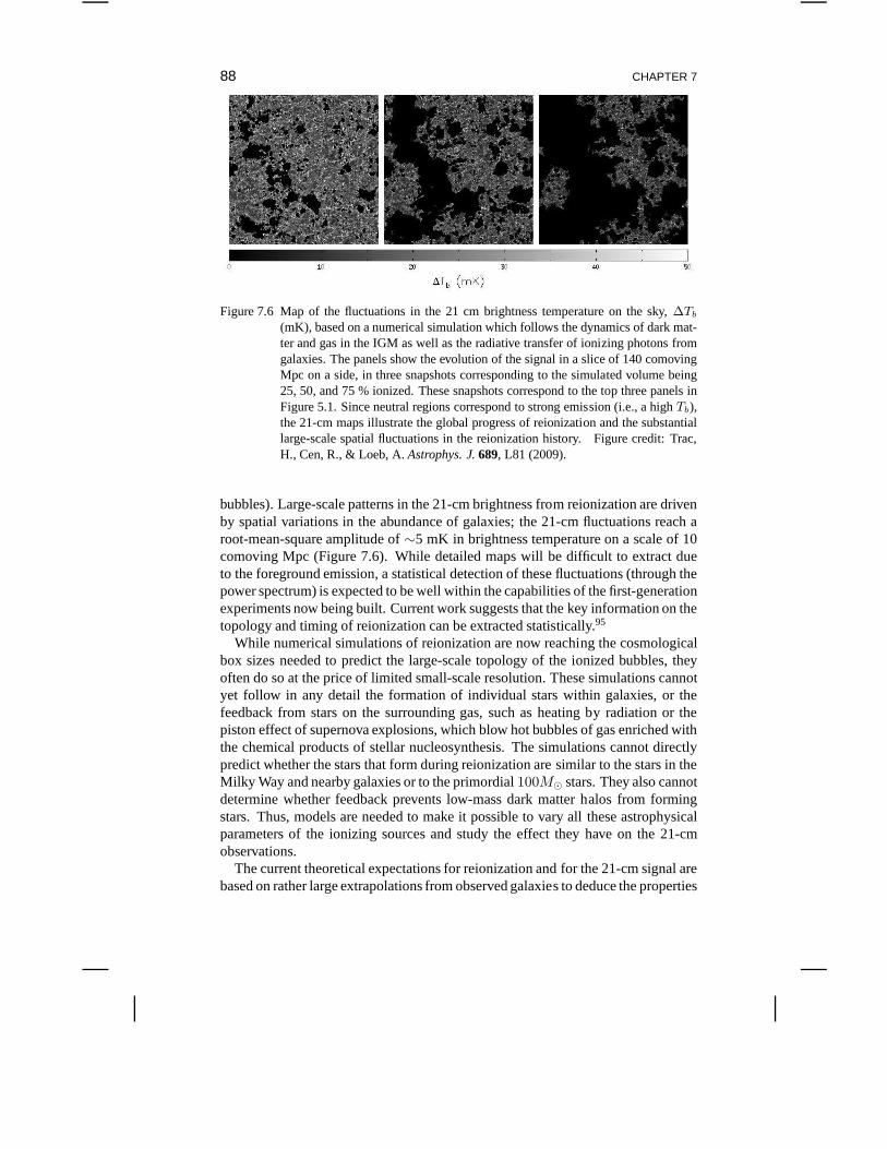
88 CHAPTER 7
Figure 7.6 Map of the fluctuations in the 21 cm brightness temperature on the sky,∆Tb
(mK), based on a numerical simulation which follows the dynamics of dark mat-ter and gas in the IGM as well as the radiative transfer of ionizing photons fromgalaxies. The panels show the evolution of the signal in a slice of 140 comovingMpc on a side, in three snapshots corresponding to the simulated volume being25, 50, and 75 % ionized. These snapshots correspond to the top three panels inFigure 5.1. Since neutral regions correspond to strong emission (i.e., a highTb),the 21-cm maps illustrate the global progress of reionization and the substantiallarge-scale spatial fluctuations in the reionization history. Figure credit: Trac,H., Cen, R., & Loeb, A.Astrophys. J.689, L81 (2009).
bubbles). Large-scale patterns in the 21-cm brightness from reionization are drivenby spatial variations in the abundance of galaxies; the 21-cm fluctuations reach aroot-mean-square amplitude of∼5 mK in brightness temperature on a scale of 10comoving Mpc (Figure 7.6). While detailed maps will be difficult to extract dueto the foreground emission, a statistical detection of these fluctuations (through thepower spectrum) is expected to be well within the capabilities of the first-generationexperiments now being built. Current work suggests that thekey information on thetopology and timing of reionization can be extracted statistically.95
While numerical simulations of reionization are now reaching the cosmologicalbox sizes needed to predict the large-scale topology of the ionized bubbles, theyoften do so at the price of limited small-scale resolution. These simulations cannotyet follow in any detail the formation of individual stars within galaxies, or thefeedback from stars on the surrounding gas, such as heating by radiation or thepiston effect of supernova explosions, which blow hot bubbles of gas enriched withthe chemical products of stellar nucleosynthesis. The simulations cannot directlypredict whether the stars that form during reionization aresimilar to the stars in theMilky Way and nearby galaxies or to the primordial100M⊙ stars. They also cannotdetermine whether feedback prevents low-mass dark matter halos from formingstars. Thus, models are needed to make it possible to vary allthese astrophysicalparameters of the ionizing sources and study the effect theyhave on the 21-cmobservations.
The current theoretical expectations for reionization andfor the 21-cm signal arebased on rather large extrapolations from observed galaxies to deduce the properties
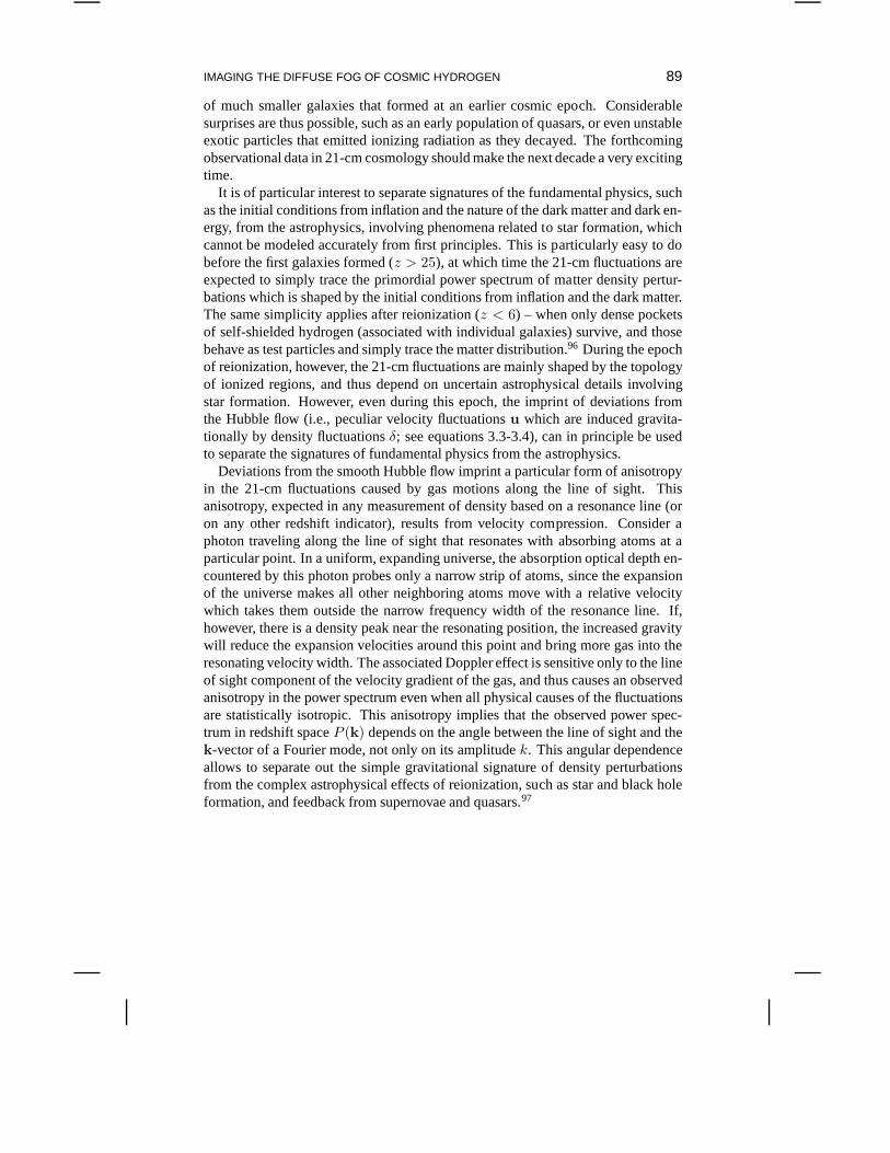
IMAGING THE DIFFUSE FOG OF COSMIC HYDROGEN 89
of much smaller galaxies that formed at an earlier cosmic epoch. Considerablesurprises are thus possible, such as an early population of quasars, or even unstableexotic particles that emitted ionizing radiation as they decayed. The forthcomingobservational data in 21-cm cosmology should make the next decade a very excitingtime.
It is of particular interest to separate signatures of the fundamental physics, suchas the initial conditions from inflation and the nature of thedark matter and dark en-ergy, from the astrophysics, involving phenomena related to star formation, whichcannot be modeled accurately from first principles. This is particularly easy to dobefore the first galaxies formed (z > 25), at which time the 21-cm fluctuations areexpected to simply trace the primordial power spectrum of matter density pertur-bations which is shaped by the initial conditions from inflation and the dark matter.The same simplicity applies after reionization (z < 6) – when only dense pocketsof self-shielded hydrogen (associated with individual galaxies) survive, and thosebehave as test particles and simply trace the matter distribution.96 During the epochof reionization, however, the 21-cm fluctuations are mainlyshaped by the topologyof ionized regions, and thus depend on uncertain astrophysical details involvingstar formation. However, even during this epoch, the imprint of deviations fromthe Hubble flow (i.e., peculiar velocity fluctuationsu which are induced gravita-tionally by density fluctuationsδ; see equations 3.3-3.4), can in principle be usedto separate the signatures of fundamental physics from the astrophysics.
Deviations from the smooth Hubble flow imprint a particular form of anisotropyin the 21-cm fluctuations caused by gas motions along the lineof sight. Thisanisotropy, expected in any measurement of density based ona resonance line (oron any other redshift indicator), results from velocity compression. Consider aphoton traveling along the line of sight that resonates withabsorbing atoms at aparticular point. In a uniform, expanding universe, the absorption optical depth en-countered by this photon probes only a narrow strip of atoms,since the expansionof the universe makes all other neighboring atoms move with arelative velocitywhich takes them outside the narrow frequency width of the resonance line. If,however, there is a density peak near the resonating position, the increased gravitywill reduce the expansion velocities around this point and bring more gas into theresonating velocity width. The associated Doppler effect is sensitive only to the lineof sight component of the velocity gradient of the gas, and thus causes an observedanisotropy in the power spectrum even when all physical causes of the fluctuationsare statistically isotropic. This anisotropy implies thatthe observed power spec-trum in redshift spaceP (k) depends on the angle between the line of sight and thek-vector of a Fourier mode, not only on its amplitudek. This angular dependenceallows to separate out the simple gravitational signature of density perturbationsfrom the complex astrophysical effects of reionization, such as star and black holeformation, and feedback from supernovae and quasars.97
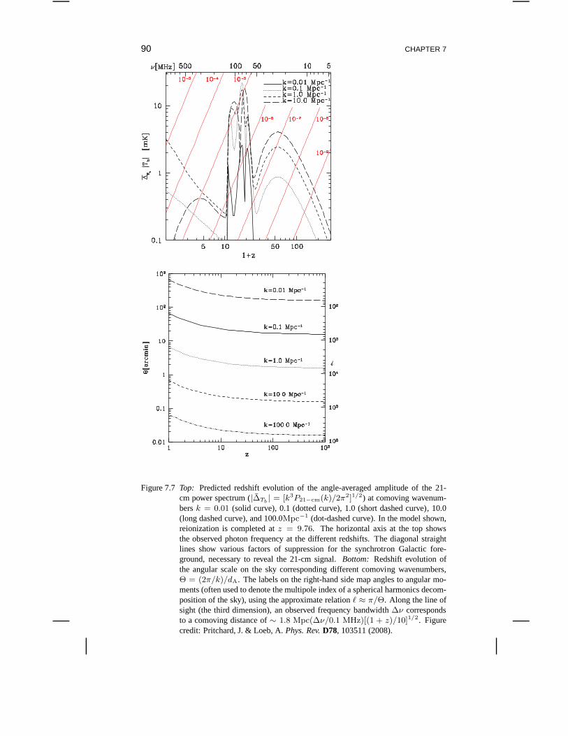
90 CHAPTER 7
Figure 7.7 Top: Predicted redshift evolution of the angle-averaged amplitude of the 21-cm power spectrum (|∆Tb
| = [k3P21−cm(k)/2π2]1/2) at comoving wavenum-bersk = 0.01 (solid curve), 0.1 (dotted curve), 1.0 (short dashed curve), 10.0(long dashed curve), and 100.0Mpc−1 (dot-dashed curve). In the model shown,reionization is completed atz = 9.76. The horizontal axis at the top showsthe observed photon frequency at the different redshifts. The diagonal straightlines show various factors of suppression for the synchrotron Galactic fore-ground, necessary to reveal the 21-cm signal.Bottom: Redshift evolution ofthe angular scale on the sky corresponding different comoving wavenumbers,Θ = (2π/k)/dA. The labels on the right-hand side map angles to angular mo-ments (often used to denote the multipole index of a spherical harmonics decom-position of the sky), using the approximate relationℓ ≈ π/Θ. Along the line ofsight (the third dimension), an observed frequency bandwidth ∆ν correspondsto a comoving distance of∼ 1.8 Mpc(∆ν/0.1 MHz)[(1 + z)/10]1/2. Figurecredit: Pritchard, J. & Loeb, A.Phys. Rev.D78, 103511 (2008).
IMAGING THE DIFFUSE FOG OF COSMIC HYDROGEN 91
7.4 OBSERVING MOST OF THE OBSERVABLE VOLUME
In general, cosmological surveys are able to measure the spatial power spectrumof primordial density fluctuations,P (k), to a precision that is ultimately limitedby Poisson statistics of the number of independent regions (the so-called “cosmicvariance”). The fractional uncertainty in the amplitude ofany Fourier mode ofwavelengthλ is given by∼ 1/
√N , whereN is the number of independent ele-
ments of sizeλ that fit within the survey volume. For the two-dimensional map ofthe CMB,N is the surveyed area of the sky divided by the solid angle occupied bya patch of areaλ2 at z ∼ 103. 21-cm observations are advantageous because theyaccess a three-dimensional volume instead of the two-dimensional surface probedby the CMB, and hence cover a larger number of independent regions in which theprimordial initial conditions were realized. Moreover, the expected 21-cm powerextends down to the pressure-dominated (Jeans) scale of thecosmic gas which is or-ders of magnitude smaller than the comoving scale at which the CMB anisotropiesare damped by photon diffusion. Consequently, the 21-cm photons can trace theprimordial inhomogeneities with a much finer resolution (i.e. many more inde-pendent pixels) than the CMB. Also, 21-cm studies promise toextend to muchhigher redshifts than existing galaxy surveys, thereby covering a much bigger frac-tion of the comoving volume of the observable Universe. At these high redshifts,small-scale modes are still in the perturbative (linear growth) regime where theirstatistical analysis is straightforward (§3). Altogether, the above factors imply thatthe 21-cm mapping of cosmic hydrogen may potentially carry the largest numberof bits of information about the initial conditions of our Universe compared to anyother survey method in cosmology.98
The limitations of existing data sets (on which the cosmological parameters inTable 3.1 are based) are apparent in Figure 2.2, which illustrates the comovingvolume of the Universe out to a redshiftz as a function ofz. State-of-the-art galaxyredshift surveys, such as the spectroscopic sample of luminous red galaxies (LRGs)in the Sloan Digital Sky Survey (SDSS), extend only out toz ∼ 0.3 (only onetenth of our horizon) and probe∼ 0.1% of the observable comoving volume ofthe Universe. Surveys of the 21-cm emission (or a large number of quasar skewersthrough the Lyman-α forest) promise to open a new window into the distributionof matter through the remaining 99.9% of the cosmic volume. These ambitiousexperiments might also probe the gravitational growth of structure through mostof the observable universe, and provide a new test of Einstein’s theory of gravityacross large scales of space and time.

Chapter Eight
Epilogue: From Our Galaxy’s Past to Its Future
The previous chapters have been dedicated to the distant past of our cosmic ances-try, when the building blocks of the Milky Way galaxy were assembled in the formof the first galaxies. The laws of physics also allow us to forecast how our Galaxyand its environment will likely change in the future. Our cosmic perspective wouldbe incomplete without a glimpse into this future.
8.1 END OF EXTRAGALACTIC ASTRONOMY
Previous generations of scholars have occasionally wondered about the long-termfuture of the Universe or in Biblical Hebrew, the forecast for “acharit hayamim”(“the end of times”). For the first time in history, we now havea standard cosmo-logical model that agrees with a large body of data about the past history of theUniverse to an unprecedented precision. This model also makes scientific predic-tions about the future. Below let us summarize those predictions for the simplestversion of the standard cosmological model with a steady cosmological constant.
Every time an American president delivers the “State of the Union” address, Iimagine what it would be like to hear a supplementary commentabout the “Stateof the Universe” surrounding the “Union”. It is, of course, completely natural fora president to focus on issues affecting re-election on a four year timescale whileignoring cosmological events that take billions of years todevelop. Nevertheless,I find it amusing to imagine a brief statement about the biggerpicture, especiallywhen we gain a significantly better understanding of our future in the cosmos thanprevious generations of astronomers had. And since cosmologists reached a majormilestone of this quality over the past decade, let us consider below what this newunderstanding of the Universe might entail for our future.
As explained in§2 and§6, cosmologists are able to observe how the Universelooked like in the past due to the finite speed of light. The light we observe todayfrom a distant source must have been emitted at an earlier time in order for it toreach us today. Hence, by looking deeper into the Universe, we can see how itlooked like at earlier times. And if we are able to measure distances, we can alsoinfer how the expansion rate of the Universe evolved with cosmic time. Naivelyone would expect the expansion to have slowed down with time because of thegravitational attraction of cosmic matter.But can this expectation be tested byobservations through telescopes?
A simple way to infer the distance of a street light with a 100-Watt bulb is tomeasure how bright it appears at night. The 100 Watts it produces are spread over
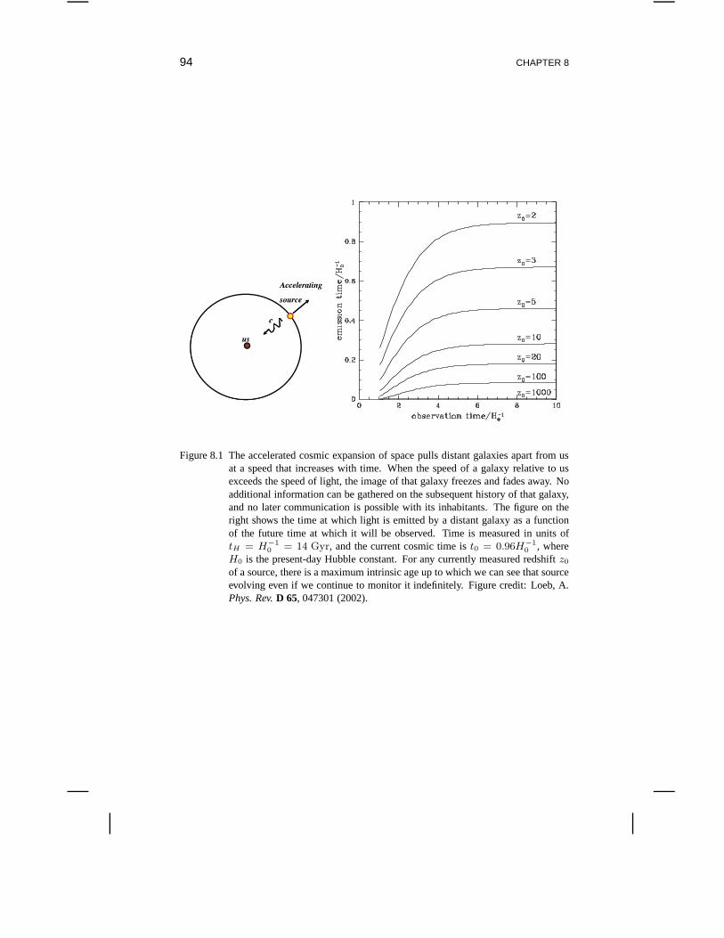
94 CHAPTER 8
Figure 8.1 The accelerated cosmic expansion of space pulls distant galaxies apart from usat a speed that increases with time. When the speed of a galaxyrelative to usexceeds the speed of light, the image of that galaxy freezes and fades away. Noadditional information can be gathered on the subsequent history of that galaxy,and no later communication is possible with its inhabitants. The figure on theright shows the time at which light is emitted by a distant galaxy as a functionof the future time at which it will be observed. Time is measured in units oftH = H−1
0= 14 Gyr, and the current cosmic time ist0 = 0.96H−1
0, where
H0 is the present-day Hubble constant. For any currently measured redshiftz0
of a source, there is a maximum intrinsic age up to which we cansee that sourceevolving even if we continue to monitor it indefinitely. Figure credit: Loeb, A.Phys. Rev.D 65, 047301 (2002).
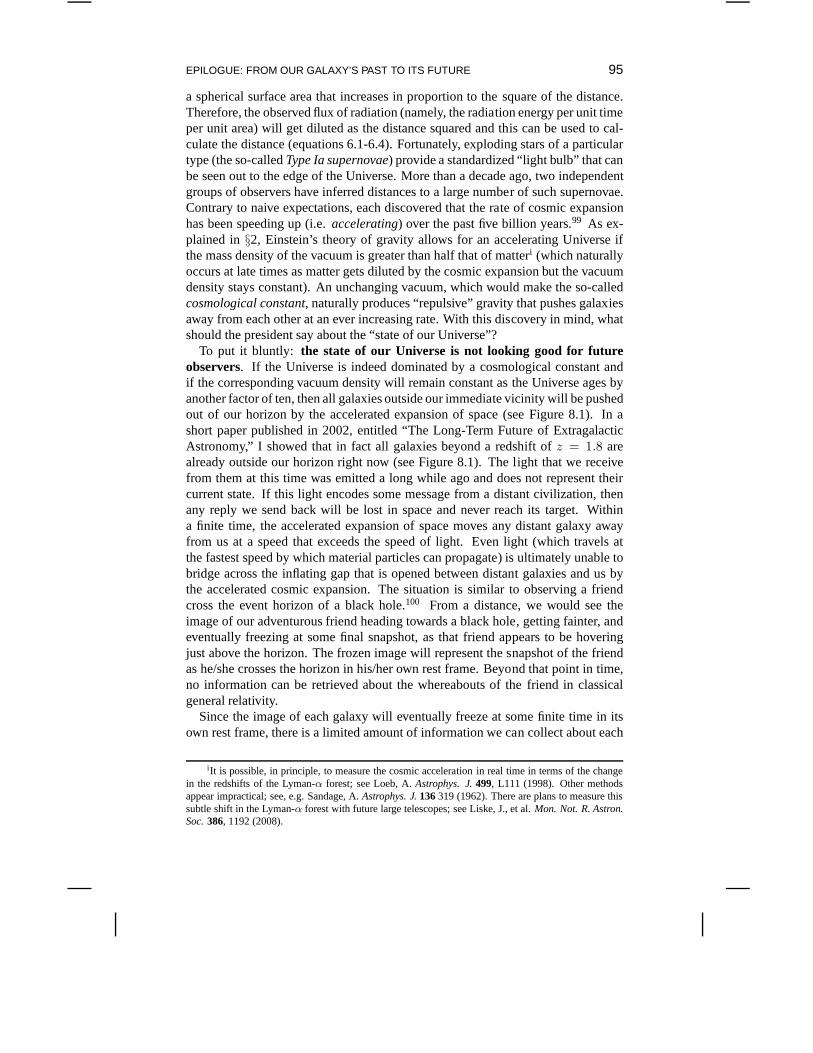
EPILOGUE: FROM OUR GALAXY’S PAST TO ITS FUTURE 95
a spherical surface area that increases in proportion to thesquare of the distance.Therefore, the observed flux of radiation (namely, the radiation energy per unit timeper unit area) will get diluted as the distance squared and this can be used to cal-culate the distance (equations 6.1-6.4). Fortunately, exploding stars of a particulartype (the so-calledType Ia supernovae) provide a standardized “light bulb” that canbe seen out to the edge of the Universe. More than a decade ago,two independentgroups of observers have inferred distances to a large number of such supernovae.Contrary to naive expectations, each discovered that the rate of cosmic expansionhas been speeding up (i.e.accelerating) over the past five billion years.99 As ex-plained in§2, Einstein’s theory of gravity allows for an accelerating Universe ifthe mass density of the vacuum is greater than half that of matteri (which naturallyoccurs at late times as matter gets diluted by the cosmic expansion but the vacuumdensity stays constant). An unchanging vacuum, which wouldmake the so-calledcosmological constant, naturally produces “repulsive” gravity that pushes galaxiesaway from each other at an ever increasing rate. With this discovery in mind, whatshould the president say about the “state of our Universe”?
To put it bluntly: the state of our Universe is not looking good for futureobservers. If the Universe is indeed dominated by a cosmological constant andif the corresponding vacuum density will remain constant asthe Universe ages byanother factor of ten, then all galaxies outside our immediate vicinity will be pushedout of our horizon by the accelerated expansion of space (seeFigure 8.1). In ashort paper published in 2002, entitled “The Long-Term Future of ExtragalacticAstronomy,” I showed that in fact all galaxies beyond a redshift of z = 1.8 arealready outside our horizon right now (see Figure 8.1). The light that we receivefrom them at this time was emitted a long while ago and does notrepresent theircurrent state. If this light encodes some message from a distant civilization, thenany reply we send back will be lost in space and never reach itstarget. Withina finite time, the accelerated expansion of space moves any distant galaxy awayfrom us at a speed that exceeds the speed of light. Even light (which travels atthe fastest speed by which material particles can propagate) is ultimately unable tobridge across the inflating gap that is opened between distant galaxies and us bythe accelerated cosmic expansion. The situation is similarto observing a friendcross the event horizon of a black hole.100 From a distance, we would see theimage of our adventurous friend heading towards a black hole, getting fainter, andeventually freezing at some final snapshot, as that friend appears to be hoveringjust above the horizon. The frozen image will represent the snapshot of the friendas he/she crosses the horizon in his/her own rest frame. Beyond that point in time,no information can be retrieved about the whereabouts of thefriend in classicalgeneral relativity.
Since the image of each galaxy will eventually freeze at somefinite time in itsown rest frame, there is a limited amount of information we can collect about each
i It is possible, in principle, to measure the cosmic acceleration in real time in terms of the changein the redshifts of the Lyman-α forest; see Loeb, A.Astrophys. J.499, L111 (1998). Other methodsappear impractical; see, e.g. Sandage, A.Astrophys. J.136319 (1962). There are plans to measure thissubtle shift in the Lyman-α forest with future large telescopes; see Liske, J., et al.Mon. Not. R. Astron.Soc.386, 1192 (2008).
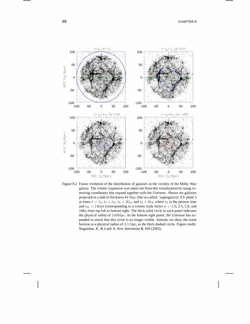
96 CHAPTER 8
-100 -50 0 50 100-100
-50
0
50
100
-100 -50 0 50 100-100
-50
0
50
100
-100 -50 0 50 100-100
-50
0
50
100
-100 -50 0 50 100-100
-50
0
50
100
Figure 8.2 Future evolution of the distribution of galaxiesin the vicinity of the Milky Waygalaxy. The cosmic expansion was taken out from this visualization by using co-moving coordinates that expand together with the Universe.Shown are galaxiesprojected in a slab of thickness 43Mpc (the so-called, ‘supergalactic XY plane’)at timest = t0, t0 + tH , t0 + 2tH , andt0 + 6tH wheret0 is the present timeandtH = 14Gyr (corresponding to a cosmic scale factora = 1.0, 2.5, 5.8, and166), from top left to bottom right. The thick solid circle ineach panel indicatesthe physical radius of143Mpc. In the bottom right panel, the Universe has ex-panded so much that this circle is no longer visible. Instead, we show the eventhorizon at a physical radius of5.1 Gpc, as the thick dashed circle. Figure credit:Nagamine, K. & Loeb A.New Astronomy8, 439 (2003).
EPILOGUE: FROM OUR GALAXY’S PAST TO ITS FUTURE 97
distant galaxy. In particular, we will never be able to studythe evolution of a galaxybeyond some finite age in its own frame of reference. The farther a galaxy is, theearlier its image freezes, and the lesser is the informationwe get about its lateevolution.
Of course, bound systems held together by a force stronger than the repulsiveforce of the cosmological constant do not participate in thecosmic expansion. Thisincludes electrons bound to atoms by the electromagnetic force, planets bound tothe Sun, as well as galaxies bound together by a stronger gravitational pull than thecosmic repulsion.
8.2 MILKY WAY + ANDROMEDA = MILKOMEDA
Which galaxies will remain gravitationally bound to the Milky Way and which willfly away? Figure 8.2 shows the results from a computer simulation of the futureevolution of all galaxies within 130 million light years of the Milky Way. Using arealization of the local distribution of galaxies based on existing observational data,the simulation predicts that all galaxies outside the localgroup of galaxies within adistance of 3 million light years are not bound to us and will be pushed out of ourview by the cosmic expansion. The gas between galaxies will get extremely cold,but remain mostly ionized, as it is today.101
How will the local group of galaxies look in the distant future? The two majorconstituents of the local group of galaxies, namely our own Milky Way galaxy andits nearest neighbor, the Andromeda galaxy (Figure 8.3), are on a collision course.The Doppler shift of spectral lines from Andromeda indicates that Andromeda andthe Milky Way are moving towards each other at a radial velocity ∼ 100 km s−1,but provides no information on the transverse speed. Other clues suggests that thetransverse speed is modest;102 the two galaxies appear to be gravitationally boundand will inevitably lose their transverse speed through dynamical friction on thedark matter around them.
For the most likely parameters of the local group, the mergerof the Milky Wayand Andromeda will take place within a few billion years (seeFigure 8.3). Sincethe lifetime of the Sun is somewhat longer,103 this event could potentially be ob-servable for future inhabitants of the solar system.What will happen to the solarsystem during the merger?Figure 8.4 shows that the Sun will most likely be kickedout to a distance that is a few times larger than its current separation from the centerof the Milky Way. During the interaction, the Milky Way mightappear as an ex-ternal galaxy to observers within the solar system. Also thenight sky will change.Currently, the thin disk of the Milky Way in which we reside appears as a stripof stars on the sky. These stars will be scattered by the merger into a spheroid-like distribution. The merger product of the collision between the Milky Way andAndromeda will make a new galaxy, which I labeled in our paperon this topicas “Milkomeda.” The spheroidal shape of Milkomeda is not unusual, as it charac-terizes a major class of galaxies called “elliptical galaxies.” Presumably, many ofthese galaxies in the present-day Universe formed out of mergers between galacticdisks at earlier cosmic times. Ultimately, only Milkomeda will remain visible to
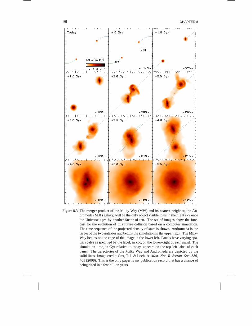
98 CHAPTER 8
Figure 8.3 The merger product of the Milky Way (MW) and its nearest neighbor, the An-dromeda (M31) galaxy, will be the only object visible to us inthe night sky oncethe Universe ages by another factor of ten. The set of images show the fore-cast for the evolution of this future collision based on a computer simulation.The time sequence of the projected density of stars is shown.Andromeda is thelarger of the two galaxies and begins the simulation in the upper right. The MilkyWay begins on the edge of the image in the lower left. Panels have varying spa-tial scales as specified by the label, in kpc, on the lower–right of each panel. Thesimulation time, in Gyr relative to today, appears on the top-left label of eachpanel. The trajectories of the Milky Way and Andromeda are depicted by thesolid lines. Image credit: Cox, T. J. & Loeb, A.Mon. Not. R. Astron. Soc.386,461 (2008). This is the only paper is my publication record that has a chance ofbeing cited in a few billion years.
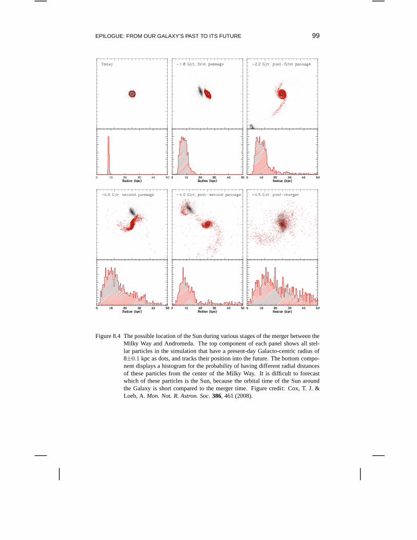
EPILOGUE: FROM OUR GALAXY’S PAST TO ITS FUTURE 99
Figure 8.4 The possible location of the Sun during various stages of the merger between theMilky Way and Andromeda. The top component of each panel shows all stel-lar particles in the simulation that have a present-day Galacto-centric radius of8±0.1 kpc as dots, and tracks their position into the future. The bottom compo-nent displays a histogram for the probability of having different radial distancesof these particles from the center of the Milky Way. It is difficult to forecastwhich of these particles is the Sun, because the orbital timeof the Sun aroundthe Galaxy is short compared to the merger time. Figure credit: Cox, T. J. &Loeb, A.Mon. Not. R. Astron. Soc.386, 461 (2008).
100 CHAPTER 8
future solar system astronomers.The current state of an accelerating Universe makes the study of cosmology a
transient episode in our long-term scientific endeavor. We better observe the Uni-verse in the next tens of billions of years and document our findings for the benefitof future scientists, who will not be able to do so. It would also seem prudent forfunding agencies to allocate their funds for cosmological observations before timeruns out. Once cosmological observations become pointless, the funds could betaken away from this line of research and be dedicated instead to solving our localpolitical problems. At that time, the future president, in giving his or her State ofthe Union address, will be fully justified in not having anything to say about theempty state of our Universe at large.
Appendix A
Notes
1de Bernardis, P., et al.Nature404, 955, (2000); Hanany, S., et al.Astrophys. J.545, L5 (2000);Miller, A. D., et al. Astrophys. J.524, L1 (1999).
2See, e.g. Peebles, P. J. E.Principles of Physical Cosmology, Princeton University Press (1993), inparticular pages 62-65.
3For advanced reading, see Mukhanov, V.Physical Foundations of Cosmology, Cambridge Univer-sity Press, Cambridge (2005).
4http://public.web.cern.ch/public/en/LHC/LHC-en.html5Loeb, A., Ferrara, A., & Ellis, R. S.First Light in the Universe, Saas-Fee Advanced Course36,
Springer, New-York (2008), and references therein.6Haiman, Z., Thoul, A. A., & Loeb, A.Astrophys. J.464, 523 (1996).7Barkana, R., & Loeb, A.Astrophys. J.523, 54 (1999).8Loeb, A., & Zaldarriaga, M.Phys. Rev.D71, 103520 (2005).9Barkana, R., & Loeb, A.Astrophys. J.531, 613 (2000), and references therein.
10Press, W. H., & Schechter, P.Astrophys. J.187, 425 (1974).11Bond, J. R., Cole, S., Efstathiou, G, & Kaiser, N.Astrophys. J.379, 440 (1991).12Lacey, C. G., & Cole, S.Mon. Not. R. Astr. Soc.262, 627 (1993).13Haiman, Z., Rees, M. J., & Loeb, A.Astrophys. J.476, 458 (1997).14Bromm, V., & Larson, R. B.Ann. Rev. Astron. & Astrophys.42, 79 (2004), and references therein.15Wyithe, J. S. B., & Loeb, A.Nature441, 322 (2006).16Munoz, J. A., Madau, P, Loeb, A., & Diemand, J.Mon. Not. R. Astron. Soc., in press (2009), and
references therein.17Turk, M. J., Abel, T., & O’Shea, BScience, in press (2009), http://arxiv.org/abs/0907.2919; Stacey,
A., Greif, T. H, & Bromm, V. Mon. Not. R., Astr. Soc.(2009), http://arxiv.org/abs/0908.0712, andreferences therein.
18Dijkstra, M., & Loeb, A.Mon. Not. R. Astron. Soc.391, 457 (2008).19Bromm, V., & Loeb, A.New Astron.9, 353 (2004).20Pudritz, R. E.Science295, 68 (2002), and references therein.21Salpeter, E.Astrophys. J.121, 161 (1955).22Rees, M. J.Mon. Not. R. Astron. Soc.176, 483 (1976).23Bromm, V., & Loeb, A.Nature425, 812 (2003).24Furlanetto, S. R., & Loeb, A.Astrophys. J.556, 619 (2001).25Furlanetto, S. R., & Loeb, A.Astrophys. J.588, 18 (2003).26Miralda-Escude, J., & Rees, M.Astrophys. J.478, L57 (2007).27Wood, K., & Loeb, A.Astrophys. J.545, 86 (2000).28Fukugita, M., Hogan, C. J., & Peebles, P. J. E.Astrophys. J.503, 518 (1998).29See, e.g. Barkana, R., & Loeb, A.Astrophys. J.539, 20 (2000); Stark, D. P., Loeb, A., & Ellis, R.
S.Astrophys. J.668, 627 (2007), and references therein.30Mo, H. J., & White, S. D. M.Mon. Not. R. Astron. Soc.336, 112 (2002).31Frebel, A., Johnson, J. L., & Bromm, V.Astrophys. J.392, L50 (2009), and references therein.32Begelman, M. C., Blandford, R. D., & Rees, M. J.Rev. Mod. Phys.56, 255 (1984).33See§14 in Shapiro, S. L., & Teukolsky, S. A.Black Holes, White Dwarfs, and Neutron Stars, Wiley,
New York (1982).34Wyithe, J. S. B., & Loeb, A.Astrophys. J.595, 614 (2003).35See Loeb, A., http://arxiv.org/abs/0909.0261 (2009), andreferences therein.36Pretorius, F.Phys. Rev. Lett.95, 121101 (2005); Campanelli, M. et al.Phys. Rev. Lett.96, 111101
(2006); Baker, J. et al.Phys. Rev. Lett.96, 111102 (2006).
102 NOTES
37Loeb, A.Phys. Rev. Lett.99, 041103 (2007).38Blecha, L., & Loeb, A.Mon. Not. R. Astr. Soc.390, 1311 (2008); Tanaka, T., & Haiman, Z.
Astrophys. J.696, 1798 (2009).39Gebhardt, K., et al.Astrophys. J.539, L13 (2000); Ferrarese, L., & Merritt, D.Astrophys. J.539,
L9 (2000). These two competing papers appeared simultaneously since I suggested the topic to theirlead authors at the same time.
40Magorrian, J., et al.Astron. J.115, 2285 (1998).41Silk, J., & Rees, M. J.Astron. & Astrophys.331, L1 (1998).42Milosavljevic, M., & Loeb, A.Astrophys. J.604, L45 (2004).43Dietrich, M., & Hamann, F.Rev. Mex. de Astron. Astrof. Conf. Ser.32, 65 (2008).44See, e.g. Wyithe, J. S. B., & Loeb, A.Astrophys. J.595, 614 (2003); Hopkins, P. F., & Hernquist,
L. Astrophys. J.698, 1550 (2009).45Genzel, R., & Karas, V. IAU Symp.238, 173 (2007); Ghez, A., et al.Astrophys. J.689, 1044
(2008).46For recent reviews about GRBs, see Meszaros, P.AIP Conf. Proc. 924, 3 (2007) &Rep. Prog.
Phys. 69, 2259 (2006) ; Piran, T.Nuovo CimentoB 121, 1039 (2006) &Rev. Mod. Phys.76, 1143(2005); and Gehrels, N., Ramirez-Ruiz, E., & Fox, D. B.Ann. Rev. Astron. & Astrophys.47, 567(2009).
47Zhang, W., Woosley, S. E., & MacFadyen, A. I.J. of Phys. Conf. Ser.46, 403 (2006)48http://swift.gsfc.nasa.gov/49Tanvir, N. R., et al.Nature, in press (2009); Salvaterra, R., et al.Nature, in press (2009).50Dunkley, J., et al.Astrophys. J. Suppl.180, 306 (2009).51Faucher-Giguere, C.-A., Lidz, A., Hernquist, L., & Zaldarriaga, M.Astrophys. J.682, L9 (2008);
Wyithe, J. S. B., & Loeb, A.Astrophys. J.586, 693 (2003).52Stromgren, B.Astrophys. J.89, 526 (1939).53Shapiro, P. R., & Giroux, M. L.Astrophys. J.321L107 (1987).54Barkana, R., & Loeb, A.Phys. Rep.349, 129 (2001), and references therein.55Wyithe, J. S. B., & Loeb, A.Nature427, 815 (2004);Astrophys. J.610, 117 (2004).56Gnedin, N.Astrophys. J.535, 530 (2000).57Barkana, R., & Loeb, A.,Astrophys. J.609, 474 (2004).58Furlanetto, S. R, Zaldarriaga, M., & Hernquist, L.Astrophys. J.613, 1 (2004).59Zahn, O., et al.Astrophys. J.654, 12 (2007).60Kaiser, N.Astrophys. J.284, L9 (1984).61Wyithe, J. S. B., & Loeb, A.Nature432, 194 (2004).62See, e.g. overview in§8 of Barkana, R., & Loeb, A.Phys. Rep.349, 125 (2000); and also Haiman,
Z., & Loeb, A.Astrophys. J.483, 21 (1997).63For an overview of the current observational status, see Ellis, R. S. (2007), http://arxiv.org/abs/astro-
ph/0701024.64Thompson, R. I.Astrophys. J.596, 748 (2003).65Bouwens, R. J., Illingworth, G. D., Franx, M., & Ford, H.Astrophys. J686, 230 (2008).66See, e.g. Kashikawa, N., et al.Astrophys. J.648, 7 (2006); Dawson, S., et al.Astrophys. J.671,
1227 (2007).67See, e.g. Yan, H., et al.Astrophys. J.651, 24 (2006); Rhoads, J. E., et al.Astrophys. J.697, 942
(2009); Ouchi, M., et al., http://arxiv.org/abs/0908.3191 (2009).68Ota, K., et al.Astrophys. J.677, 12 (2008).69Bradley, L., et al.Astrophys. J.678, 647 (2008).70Stark, D., et al.Astrophys. J.663, 10 (2007); Bouwens, R. J., et al.Astrophys. J690, 1764 (2009).71Ciardi, B., & Loeb, A.Astrophys. J.540, 687 (2000).72Barkana, R., & Loeb, A.Astrophys. J.601, 64 (2004).73Bromm, V., & Loeb, A.Astrophys. J.642382 (2006).74See, e.g. Barkana, R., & Loeb, A.Astrophys. J.531, 613 (2000) and539, 20 (2000).75Bromm, V., Kudritzki, R. P., & Loeb, A.Astrophys. J.552, 464 (2001).76http://www.eso.org/sci/facilities/eelt/77http://www.gmto.org/78http://www.tmt.org/79Wyithe, J. S. B., & Loeb, A.Mon. Not. R. Astron. Soc.375, 1034 (2007).80http://almaobservatory.org/
103
81Scheuer, P. A. G.Nature207, 963 (1965).82Gunn, J. E., & Peterson, B. A.Astrophys. J.142, 1633 (1965).83Miralda-Escude, J.Astrophys. J.501, 15 (1998).84For further reading on 21-cm cosmology, see Furlanetto, S. R., Oh, S. P., & Briggs, F. H.Phys.
Rep.433, 181 (2006), and references therein.85Loeb, A., & Zaldarriaga, M.Phys. Rev. Lett.92, 211301 (2004).86Wouthuysen, S. A.Astron. J.57, 31 (1952); Field, G. B.Proc. IRE46, 240 (1958).87Madau, P., Meiksin, A., & Rees, M. J.Astrophys. J.475, 429 (1997).88Scott, D., & Rees, M. J.Mon. Not. R. Astron. Soc.247, 510 (1990).89http://www.lofar.org/90http://www.haystack.mit.edu/ast/arrays/mwa/site/index.html91http://arxiv.org/abs/astro-ph/050202992http://arxiv.org/abs/0904.233493http://www.skatelescope.org94See, e.g. Bowman, J. D., Rogers, A. E. E., & Hewitt, J. N.Astrophys. J.676, 1 (2008).95See, e.g. Lidz, A., Zahn, O., McQuinn, M., Zaldarriaga, M., &Hernquist, L.Astrophys. J.680, 962
(2008), and references therein.96Wyithe, J. S. B. & Loeb, A.Mon. Not. R. Astr. Soc.383, 1195 (2008).97Barkana, R., & Loeb, A.Astrophys. J.624, L65 (2005).98Loeb, A., & Wyithe, J. S. B.Phys. Rev. Lett.100, 161301 (2008); Mao, Y., et al.Phys. Rev.D78,
023529 (2008).99Riess, A., et al.Astron. J.116, 1009 (1998); Perlmutter, S., et al.Astrophys. J.517, 565 (1999).
100For further reading on black hole horizons, see Thorne, K. S.Black Holes and Time Warps, W. W.Norton & Company, New York (1994).
101Nagamine, K. & Loeb A.New Astronomy9, 573 (2004).102van der Marel, R. P., & Guhathakurta, P.Astrophys. J.678, 187 (2008); Loeb, A. Reid, M., Brun-
thaler, A., & Falcke, H.Astrophys. J.633, 894 (2005).103Schroder, P., & Connon Smith, R.Mon. Not. R. Astron. Soc.386, 155 (2008).

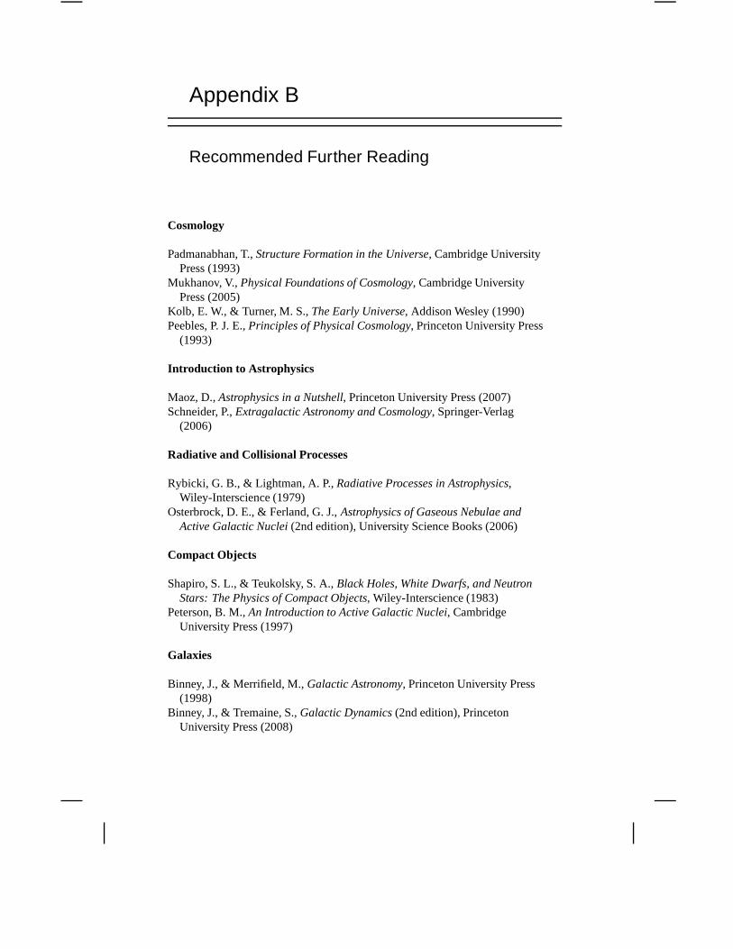
Appendix B
Recommended Further Reading
Cosmology
Padmanabhan, T.,Structure Formation in the Universe, Cambridge UniversityPress (1993)
Mukhanov, V.,Physical Foundations of Cosmology, Cambridge UniversityPress (2005)
Kolb, E. W., & Turner, M. S.,The Early Universe, Addison Wesley (1990)Peebles, P. J. E.,Principles of Physical Cosmology, Princeton University Press
(1993)
Introduction to Astrophysics
Maoz, D.,Astrophysics in a Nutshell, Princeton University Press (2007)Schneider, P.,Extragalactic Astronomy and Cosmology, Springer-Verlag
(2006)
Radiative and Collisional Processes
Rybicki, G. B., & Lightman, A. P.,Radiative Processes in Astrophysics,Wiley-Interscience (1979)
Osterbrock, D. E., & Ferland, G. J.,Astrophysics of Gaseous Nebulae andActive Galactic Nuclei(2nd edition), University Science Books (2006)
Compact Objects
Shapiro, S. L., & Teukolsky, S. A.,Black Holes, White Dwarfs, and NeutronStars: The Physics of Compact Objects, Wiley-Interscience (1983)
Peterson, B. M.,An Introduction to Active Galactic Nuclei, CambridgeUniversity Press (1997)
Galaxies
Binney, J., & Merrifield, M.,Galactic Astronomy, Princeton University Press(1998)
Binney, J., & Tremaine, S.,Galactic Dynamics(2nd edition), PrincetonUniversity Press (2008)


Appendix C
Useful Numbers
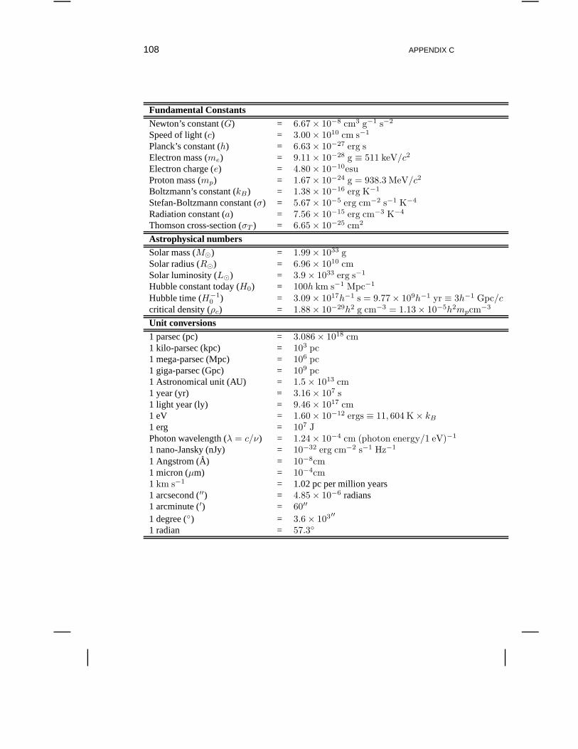
108 APPENDIX C
Fundamental Constants
Newton’s constant (G) = 6.67 × 10⁻⁸ cm3 g−1 s−2
Speed of light (c) = 3.00 × 1010 cm s−1
Planck’s constant (h) = 6.63 × 10⁻²⁷ erg sElectron mass (me) = 9.11 × 10⁻²⁸ g ≡ 511 keV/c2
Electron charge (e) = 4.80 × 10⁻¹⁰esuProton mass (mp) = 1.67 × 10⁻²⁴ g = 938.3 MeV/c2
Boltzmann’s constant (kB) = 1.38 × 10⁻¹⁶ erg K−1
Stefan-Boltzmann constant (σ) = 5.67 × 10⁻⁵ erg cm−2 s−1 K−4
Radiation constant (a) = 7.56 × 10⁻¹⁵ erg cm−3 K−4
Thomson cross-section (σT ) = 6.65 × 10⁻²⁵ cm2
Astrophysical numbersSolar mass (M⊙) = 1.99 × 1033 gSolar radius (R⊙) = 6.96 × 10¹⁰ cmSolar luminosity (L⊙) = 3.9 × 1033 erg s−1
Hubble constant today (H0) = 100h km s−1 Mpc−1
Hubble time (H−10 ) = 3.09 × 10¹⁷h−1 s = 9.77 × 10⁹h−1 yr ≡ 3h−1 Gpc/c
critical density (ρc) = 1.88 × 10⁻²⁹h2 g cm−3 = 1.13 × 10⁻⁵h2mpcm−3
Unit conversions
1 parsec (pc) = 3.086 × 1018 cm1 kilo-parsec (kpc) = 103 pc1 mega-parsec (Mpc) = 106 pc1 giga-parsec (Gpc) = 109 pc1 Astronomical unit (AU) = 1.5 × 1013 cm1 year (yr) = 3.16 × 10⁷ s1 light year (ly) = 9.46 × 1017 cm1 eV = 1.60 × 10⁻¹² ergs ≡ 11, 604 K × kB
1 erg = 107 JPhoton wavelength (λ = c/ν) = 1.24 × 10⁻⁴ cm (photon energy/1 eV)−1
1 nano-Jansky (nJy) = 10−32 erg cm−2 s−1 Hz−1
1 Angstrom (A) = 10−8cm1 micron (µm) = 10−4cm1 km s−1 = 1.02 pc per million years1 arcsecond (′′) = 4.85 × 10⁻⁶ radians1 arcminute (′) = 60′′
1 degree () = 3.6 × 10³′′
1 radian = 57.3
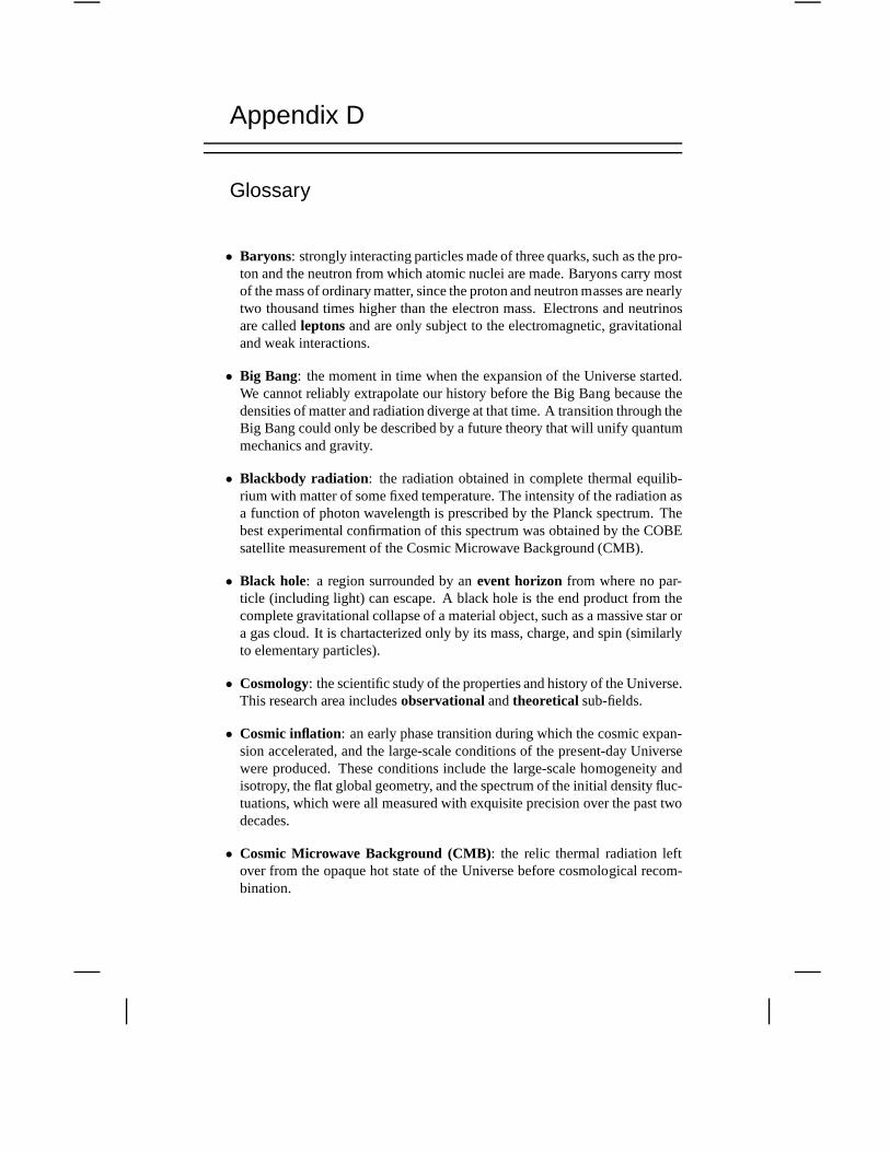
Appendix D
Glossary
• Baryons: strongly interacting particles made of three quarks, suchas the pro-ton and the neutron from which atomic nuclei are made. Baryons carry mostof the mass of ordinary matter, since the proton and neutron masses are nearlytwo thousand times higher than the electron mass. Electronsand neutrinosare calledleptonsand are only subject to the electromagnetic, gravitationaland weak interactions.
• Big Bang: the moment in time when the expansion of the Universe started.We cannot reliably extrapolate our history before the Big Bang because thedensities of matter and radiation diverge at that time. A transition through theBig Bang could only be described by a future theory that will unify quantummechanics and gravity.
• Blackbody radiation: the radiation obtained in complete thermal equilib-rium with matter of some fixed temperature. The intensity of the radiation asa function of photon wavelength is prescribed by the Planck spectrum. Thebest experimental confirmation of this spectrum was obtained by the COBEsatellite measurement of the Cosmic Microwave Background (CMB).
• Black hole: a region surrounded by anevent horizon from where no par-ticle (including light) can escape. A black hole is the end product from thecomplete gravitational collapse of a material object, suchas a massive star ora gas cloud. It is chartacterized only by its mass, charge, and spin (similarlyto elementary particles).
• Cosmology: the scientific study of the properties and history of the Universe.This research area includesobservationalandtheoretical sub-fields.
• Cosmic inflation: an early phase transition during which the cosmic expan-sion accelerated, and the large-scale conditions of the present-day Universewere produced. These conditions include the large-scale homogeneity andisotropy, the flat global geometry, and the spectrum of the initial density fluc-tuations, which were all measured with exquisite precisionover the past twodecades.
• Cosmic Microwave Background (CMB): the relic thermal radiation leftover from the opaque hot state of the Universe before cosmological recom-bination.
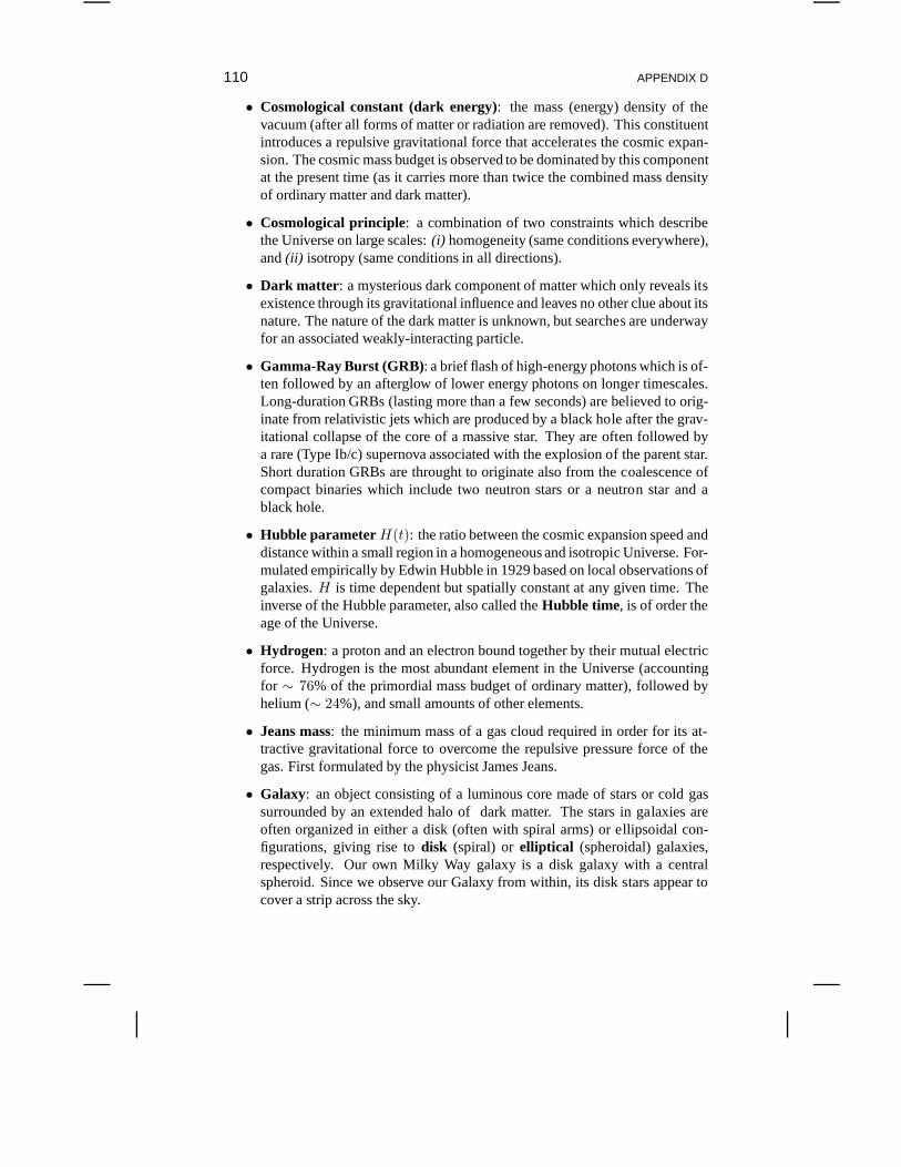
110 APPENDIX D
• Cosmological constant (dark energy): the mass (energy) density of thevacuum (after all forms of matter or radiation are removed).This constituentintroduces a repulsive gravitational force that accelerates the cosmic expan-sion. The cosmic mass budget is observed to be dominated by this componentat the present time (as it carries more than twice the combined mass densityof ordinary matter and dark matter).
• Cosmological principle: a combination of two constraints which describethe Universe on large scales:(i) homogeneity (same conditions everywhere),and(ii) isotropy (same conditions in all directions).
• Dark matter : a mysterious dark component of matter which only reveals itsexistence through its gravitational influence and leaves noother clue about itsnature. The nature of the dark matter is unknown, but searches are underwayfor an associated weakly-interacting particle.
• Gamma-Ray Burst (GRB): a brief flash of high-energy photons which is of-ten followed by an afterglow of lower energy photons on longer timescales.Long-duration GRBs (lasting more than a few seconds) are believed to orig-inate from relativistic jets which are produced by a black hole after the grav-itational collapse of the core of a massive star. They are often followed bya rare (Type Ib/c) supernova associated with the explosion of the parent star.Short duration GRBs are throught to originate also from the coalescence ofcompact binaries which include two neutron stars or a neutron star and ablack hole.
• Hubble parameter H(t): the ratio between the cosmic expansion speed anddistance within a small region in a homogeneous and isotropic Universe. For-mulated empirically by Edwin Hubble in 1929 based on local observations ofgalaxies.H is time dependent but spatially constant at any given time. Theinverse of the Hubble parameter, also called theHubble time, is of order theage of the Universe.
• Hydrogen: a proton and an electron bound together by their mutual electricforce. Hydrogen is the most abundant element in the Universe(accountingfor ∼ 76% of the primordial mass budget of ordinary matter), followed byhelium (∼ 24%), and small amounts of other elements.
• Jeans mass: the minimum mass of a gas cloud required in order for its at-tractive gravitational force to overcome the repulsive pressure force of thegas. First formulated by the physicist James Jeans.
• Galaxy: an object consisting of a luminous core made of stars or coldgassurrounded by an extended halo of dark matter. The stars in galaxies areoften organized in either a disk (often with spiral arms) or ellipsoidal con-figurations, giving rise todisk (spiral) or elliptical (spheroidal) galaxies,respectively. Our own Milky Way galaxy is a disk galaxy with acentralspheroid. Since we observe our Galaxy from within, its disk stars appear tocover a strip across the sky.
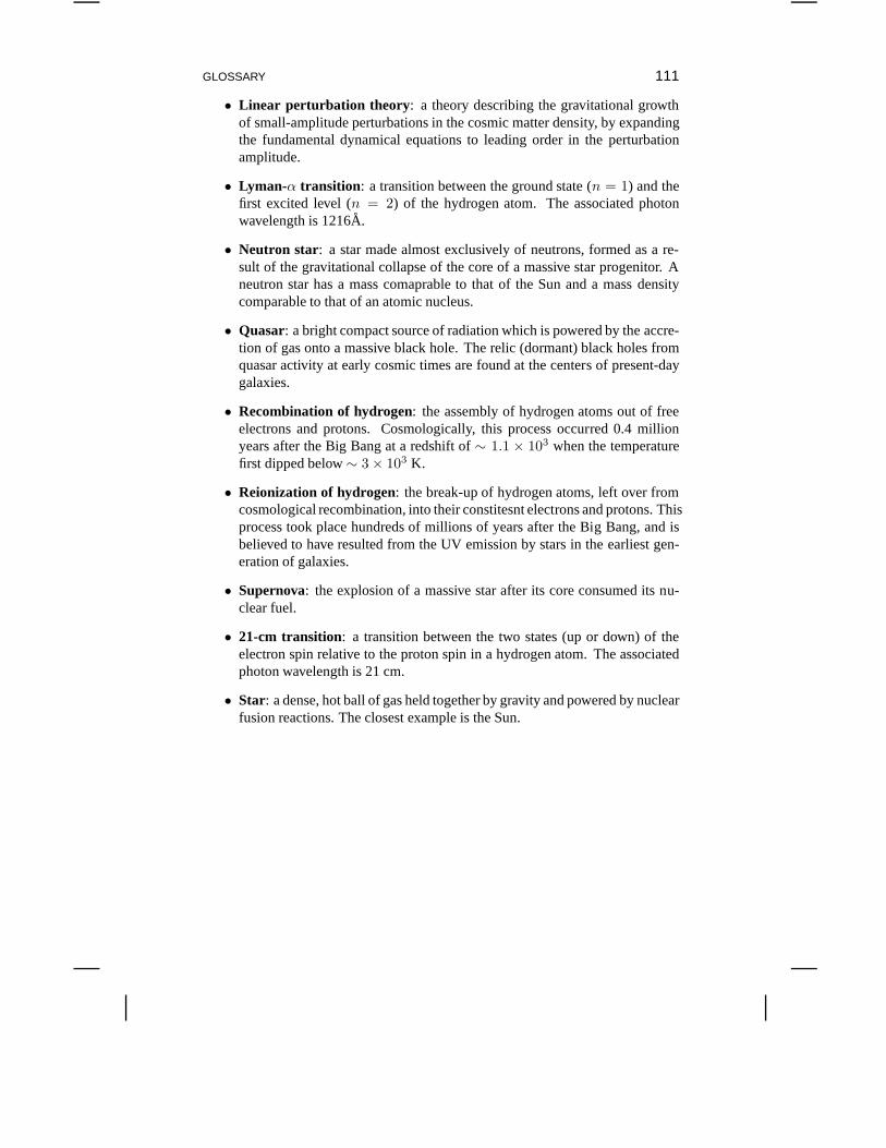
GLOSSARY 111
• Linear perturbation theory : a theory describing the gravitational growthof small-amplitude perturbations in the cosmic matter density, by expandingthe fundamental dynamical equations to leading order in theperturbationamplitude.
• Lyman-α transition : a transition between the ground state (n = 1) and thefirst excited level (n = 2) of the hydrogen atom. The associated photonwavelength is 1216A.
• Neutron star: a star made almost exclusively of neutrons, formed as a re-sult of the gravitational collapse of the core of a massive star progenitor. Aneutron star has a mass comaprable to that of the Sun and a massdensitycomparable to that of an atomic nucleus.
• Quasar: a bright compact source of radiation which is powered by theaccre-tion of gas onto a massive black hole. The relic (dormant) black holes fromquasar activity at early cosmic times are found at the centers of present-daygalaxies.
• Recombination of hydrogen: the assembly of hydrogen atoms out of freeelectrons and protons. Cosmologically, this process occurred 0.4 millionyears after the Big Bang at a redshift of∼ 1.1 × 10³ when the temperaturefirst dipped below∼ 3 × 10³ K.
• Reionization of hydrogen: the break-up of hydrogen atoms, left over fromcosmological recombination, into their constitesnt electrons and protons. Thisprocess took place hundreds of millions of years after the Big Bang, and isbelieved to have resulted from the UV emission by stars in theearliest gen-eration of galaxies.
• Supernova: the explosion of a massive star after its core consumed its nu-clear fuel.
• 21-cm transition: a transition between the two states (up or down) of theelectron spin relative to the proton spin in a hydrogen atom.The associatedphoton wavelength is 21 cm.
• Star: a dense, hot ball of gas held together by gravity and poweredby nuclearfusion reactions. The closest example is the Sun.

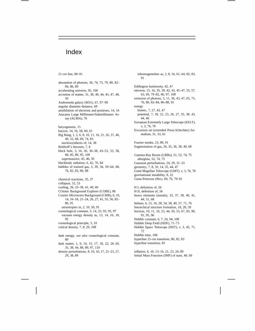
Index
21-cm line, 80–91
absorption of photons, 36, 74, 75, 79, 80, 82–84, 86, 89
accelerating universe, 95, 100accretion of matter, 31, 38, 40, 44, 45, 47, 48,
50Andromeda galaxy (M31), 67, 97–99angular diameter distance, 69annihilation of electrons and positrons, 14, 16Atacama Large Millimeter/Submillimeter Ar-
ray (ALMA), 76
baryogenesis, 15baryon, 14, 16, 58, 60, 61Big Bang, 1, 2, 6, 8, 10, 11, 16, 21, 26, 37, 46,
49, 55, 68, 69, 74, 83nucleosynthesis of, 14, 38
Birkhoff’s theorem, 7, 8black hole, 3, 16, 26, 36–38, 43–53, 55, 58,
68, 85, 89, 95, 109supermassive, 45, 46, 50
blackbody radiation, 6, 42, 76, 84bubbles of ionized gas, 3, 39, 56, 59–64, 68,
76, 82, 83, 86, 88
chemical reactions, 35, 37collapsar, 52, 53cooling, 26, 33–38, 41, 49, 60COsmic Background Explorer (COBE), 86Cosmic Microwave Background (CMB), 6, 10,
14, 16–18, 21–24, 26, 27, 41, 55, 56, 82–86, 91
anisotropies in, 2, 10, 56, 91cosmological constant, 5, 14, 23, 93, 95, 97
vacuum energy density as, 13, 14, 16, 18,95
cosmological principle, 5, 10critical density, 7, 8, 29, 108
dark energy,see alsocosmological constant,89
dark matter, 1, 9, 14, 15, 17, 18, 22, 26–29,35, 38, 44, 88, 89, 97, 110
density perturbations, 8, 10, 16, 17, 21–23, 27,29, 38, 89
inhomogeneities as, 2, 8, 16, 61, 64, 82, 83,91
Eddington luminosity, 42, 47electron, 15, 16, 35, 39, 42, 43, 45–47, 55, 57,
63, 69, 79–82, 86, 97, 108emission of photons, 3, 11, 36, 43, 47, 65, 75,
76, 80, 82–84, 86–88, 91energy
kinetic, 7, 27, 43, 47potential, 7, 18, 22, 23, 26, 27, 35, 38, 43,
44, 46European Extremely Large Telescope (EELT),
v, 3, 76, 78Excursion set (extended Press-Schechter) for-
malism, 31, 33, 61
Fourier modes, 23, 89, 91fragmentation of gas, 26, 35, 36, 38, 49, 68
Gamma-Ray Bursts (GRBs), 51, 52, 74, 75afterglow, 52, 74, 75
Gaussian perturbations, 24, 29, 31–33geometry, 7, 8, 10, 14, 35, 44, 47Giant Magellan Telescope (GMT), v, 3, 76, 78gravitational instability, 8, 22Gunn-Peterson effect, 69, 76, 79–81
H I, definition of, 56H II, definition of, 56heavy elements (metals), 33, 37, 38, 40, 41,
44, 51, 68helium, 6, 15, 16, 28, 34, 38, 40, 57, 71, 76hierarchical structure formation, 18, 28, 59horizon, 10, 11, 16, 23, 44, 50, 55, 67, 85, 90,
91, 95, 96Hubble constant, 6, 7, 24, 94, 108Hubble Deep Field (HDF), 71–73Hubble Space Telescope (HST), v, 3, 45, 71,
72Hubble time, 108hyperfine 21-cm transition, 80, 82, 83hyperfine transition, 83
inflation, 6, 10, 13–16, 21, 23, 24, 89Initial Mass Function (IMF) of stars, 40, 69
114 INDEX
intergalactic medium (IGM), 18, 19, 42, 56,57, 59–61, 64, 79–84, 88
interstellar medium (ISM), 33, 37, 57, 71, 76ionized regions, 39, 59, 61, 84, 85
James Webb Space Telescope (JWST), v, 3,75, 76
Jeans mass, 26, 27, 35, 36, 38, 40, 43, 64, 91
large-scale structure, 2, 17, 22, 24, 64, 79Low Frequency Array (LOFAR), 86luminosity, 42, 43, 46–48, 61, 69, 71luminosity distance, 69Lyman-α forest, 24, 63, 79, 91, 95Lyman-α line, 79–82, 84, 95
metallicity, 40, 41, 43Milkomeda galaxy, 97Milky Way, 1, 2, 5, 6, 8, 17, 21, 33, 38, 40, 44,
48, 50, 51, 67, 68, 82, 86, 88, 93, 96–99molecules, 28, 33–35, 37–39, 41, 48Murchison Wide-Field Array (MWA), 86, 87
nano-Jansky (nJy), 69, 108neutral hydrogen (H I), 3, 16, 56, 76, 82, 84neutrino, 15–17neutron, 14–16, 37, 38, 52neutron star, 37NFW density profile, 28nucleosynthesis, 14, 38, 88numerical simulations, 4, 21, 27–31, 33, 35,
36, 38, 39, 41, 44, 47–49, 62–64, 68, 88,97–99
overdensity, 8, 9, 21, 27, 29, 31, 62–64, 79, 84
parsec, 108peculiar velocity, 22, 89photometry, 80, 81photon, 11, 13, 14, 16, 17, 35, 42, 43, 47, 51,
52, 55–64, 69, 74, 80, 82–85, 89, 91energy of, 108frequency of, v, 3, 11, 71, 80, 82–87, 89, 90wavelength of, 11, 43, 80, 108
Planck satellite, 55Planck time, 16Poisson’s equation, 22polarization, 55Populations of stars
Population I, 40Population II, 40, 42, 43Population III, 40, 42, 43, 47, 56, 75
positron, 16, 43, 45power spectrum, 23, 24, 29, 61, 88, 90, 91Precision Array to Probe the Epoch of Reion-
ization (PAPER), 86Press-Schechter model, 29, 31, 32, 59, 60, 62Primeval Structure Telescope, 86
primordial gas, 28, 35, 38, 41, 68, 75proton, 14–16, 28, 42, 45, 46, 55, 56, 63, 64,
79–81, 108
quark, 15, 16quasar, 44–48, 51, 55, 56, 58, 59, 61, 74, 75,
79–81, 89, 91
radio, v, 3, 45, 52, 65, 76, 84, 86, 87recombination, 12, 15, 19, 21, 22, 35, 43, 55–
61, 63, 83, 85reionization, 12, 38, 43, 55, 56, 59–65, 67, 68,
76, 79–82, 84–86, 88–90rotation, 26, 45, 50, 81
Salpeter mass function, 40, 69Sloan Digital Sky Survey (SDSS), 81, 91sound waves, 10, 11, 24spectroscopy, 74–76, 80, 81, 91spherical collapse, 26, 28, 29, 31
turnaround of, 27spin temperature, 83–85Spitzer Space Telescope, 72Square Kilometer Array (SKA), 86Sun, 1, 3, 17, 27, 38, 40, 42, 68, 75, 97
abundance in, 42, 44luminosity of, 108mass of, 25, 108radius of, 42, 108
supermassive star, 48, 49supernova, 28, 37, 38, 41, 43, 48, 52, 68, 74,
85, 88, 89, 95pair instability, 43
synchrotron radiation, 86, 90
Thirty Meter Telescope (TMT), v, 3, 76, 78Thomson cross-section, 46, 55, 108
virial parameters, 26–29, 34, 35, 48, 49, 61
Wilkinson Microwave Anisotropy Probe (WMAP),2, 55, 56
Wouthuysen-Field effect, 84