ORIGlr~AL

THE HOUSEHOLD LIFE CYCLE AND HOUSING CHOICES

Kevin F. McCarthy

January 1976

P-5565

The Rand Paper Series

Papers are issued by The Rand Corporation as a service to its professional staff.Their purpose is to facilitate the exchange of ideas among those who share theauthor's research interests; Papers are not reports prepared in fulfillment ofRand's contracts or grants. Views expressed in a Paper are the author's own, andare not necessarily shared by Rand or its research sponsors.

The Rand CorporationSanta Monica, California 90406

Kevin F. McCarthy

The Rand Corporation, Santa Monica, California

INTRODUCTION

The Housing Assistance Supply Experiment is designed to test the

effects on local housing markets of a full-scale program of housing

allowances for low-income households. A test is important because,

unlike most housing assistance programs, this one is administered

largely by its beneficiaries, operating through normal market channels.

Within limits, a program participant is free to choose the type

and quality of ho~sing and the form of tenure that suit his preferences

and his allowance-augmented budget. The administering agency assists

with a monthly payment whose amount does not depend on these decisions,

requiring of the recipient only that he occupy housing that meets min­

imum standards of space and habitability.

To understand how the allowance payments and related program rules

affect participants' housing choices, it is first necessary to under­

stand the structure of those choices in the absence of an allowance

program. This paper summarizes what we have learned so far from pre­

program interviews with homeowners and renters in Brown County, Wiscon­

sin, the first of our two experimental sites.

The analysis reported here is preliminary'to building an integrated

and, we hope, fairly general model of the determinants of the kinds of

housing choices open to program participants: tenure, type and quality

of housing, housing expenditures, and location of residence.

*This paper was prepared for presentation at the twenty-secondNorth American Meeting of the Regional Science Association in Cambridge,Massachusetts, on 7 November 1975. It draws on research conducted byThe Rand Corporation as part of the Housing Assistance Supply Experiment.That research was sponsored and funded by the Office of Policy Develop­ment and Research, U.S. Department of Housing and Urban Development,under Contract No. H-1789. Views and conclusions expressed herein aretentative and do not represent the official opinion of the sponsoringagency.

The author gratefully acknowledges the assistance of Ira S. Lowryand C. Lance Barnett in preparing this paper.

~-2-

,I

------------

The major theme of this paper is that housing choices are power­

fully conditioned by the demographic configuration of the household,

as measured jointly by the marital status and ages of the household

heads, the presence of children in the household, and the age of the

youngest child. These configurations are denoted here as stages in the

household life cycle. The paper shows how housing characteristics and

changes of residence in Brown County, Wisconsin, vary with life-cycle

stage, controlling for income differences where appropriate and possible.

The life-cycle approach to the study of housing consumption and

its adjustments over time is not new. Lansing and Kish [12], Lansing

and Morgan [11], and David [5] have demonstrated the variability of

consumption patterns over the household life cycle, while Speare [19],

Chevan [4], Guest [9], and Pickvance [14] have demonstrated the rela­

tionship between the life cycle, housing consumption, and local mobil­

ity. Most analyses of housing consumption patterns that do not

explicitly include a life-cycle variable (Kain and Quigley [10]; Struyk

and Marshall [20]) use some of its component measures as separate ex­

planatory factors. The approach used here differs from these studies

partly in emphasis and partly in the amount of detail afforded by our

data base.

The remainder of this paper is divided into five parts. The first

part describes the data base on which the analysis draws and comments

on its statistical properties. The second part classifies households

in Brown County by life-cycle stage and shows how a number of consumption­

related household characteristics vary by stage. The third part examines

differences in current housing consumption by life-cycle stage and in­

come. The fourth part deals with changes of residence as the principal

means by which households adjust their housing consumption to changes

in their circumstances. The last part summarizes our principal findings

and lists topics for future research.

THE DATA BASE AND STATISTICAL ISSUES

The data used for this analysis were produced by the survey of ten­

ants and homeowners conducted in Brown County from December 1973 through

April 1974. This survey was conducted on a multi-stage stratified cluster

-3-

sample of 3,722 households, the records of which were then weighted

to represent approximately 42,600 comparable households in the county's

population. The population represented by our sample excludes roughly1

12 percent of all Brown County households. The largest excluded group

consists of about 3,200 households containing landlords (or their

agents); persons to be interviewed as landlords were deliberately skipped

by the survey of tenants and homeowners. Another excluded group consists

of some 1,300 occupants of federally subsidized housing units, also de­

liberately skipped by the survey; the majority of these are homeowners

receiving mortgage assistance. Finally, residents of mobile homes and

lodgers in rooming houses and private homes, although interviewed, pre­

sented special data processing problems and are excluded from the data

base used here; they represent a population of about 1,300 households.

Although these excluded households may differ in some respects from the

population covered by our sample, for simplicity in exposition we will

refer to the sampled population as though it fully represented Brown

County.

In conducting our analysis we were confronted with the problem of

missing data, particularly on income and expense items. Consequently,

the results reported here pertain to three different sets of records.

For general descriptions of households and their housing, the full set

of 3,722 records (887 owners and 2,835 renters) was used. In examin­

ing the income characteristics of households, only the 3,223 records

containing complete income information were used (733 owners and 2,490

renters). In examining the relationship between renters' housing ex­

penses and income, only the 2,326 records containing both income and

IA household is a person living alone or a group of people whoshare a housing unit--i.e., share a room or group of rooms intendedfor occupancy as a separate living quarters with complete kitchen fa­cilities and direct access to the unit either through the outside ofa unit or through a common hall. Usually, but not necessarily, membersof a household are related by blood or marriage. The related membersof a household constitute a family. Individuals not living in house­holds consist of transients, persons living in group quarters such asstudent dormitories, and inmates of institutions such as hospitalsor prisons.

-4-

expense data were used. In each case, population weights were recal­

culated for respondents in each of 16 sampling strata, to compensate

for nonresponse in that stratum. An audit of within-stratum nonresponse

patterns does not reveal any biases serious enough to affect interpre­

tation of the findings reported here.

Most of the data presented are in the form of cross-tabulations.

The entries in these tabulations are population estimates from sample

data and are thus subject to sampling error in addition to the sampling

exclusions and possible nonresponse biases noted above. Because of the

structure of the sample, calculating accurate variances for population

estimates is an extremely complex procedure, the software for which is

still being developed. We are as yet unable to test reliably for the

statistical significance of differences between estimated population

parameters, depending instead on conservative interpretations of the

evidence.2

To enable the reader to make independent judgments, each

table reports the number of observations on which its entries are

based, and all entries based on fewer than ten observations are flagged.

THE HOUSEHOLD LIFE CYCLE IN BROWN COUNTY

Households in Brown County are similar to those of most other

small metropolitan areas in that they are somewhat larger than house­

holds in the nation as a whole (3.4 vs. 3.0 persons), more likely to

consist of married couples (75 percent vs. 67 percent), and have younger3heads (42.7 years vs. 47.3 years). The most notable characteristic of

Brown County's households that relates to housing choices is their racial

and ethnic homogeneity. Over 98 percent of all household heads are white

(vs. 89 percent nationally) and approximately two-thirds report ethnic

origins in northern Europe. The only conspicuous minority group con­

sists of American Indians (about 1.5 percent of the county's population),

most of whom live in tribal lands in the rural part of the county. This

2Given that this preliminary analysis is designed primarily to guidesubsequent model specification by revealing any strong patterns in thedata, significance testing at this stage is not crucial to uur purposes.

3The data on the national population of households are taken fromU.S. Bureau of the Census [23J.

-5-

lack of racial and ethnic diversity eliminates from Brown County an

important differentiating factor which many analysts have found to

be important to the operation of the housing market in more hetero­

geneous communities.

Differences between households within Brown County are, of course,

considerably more important to local consumption patterns than differ­

ences between local and national averages. In an attempt to identify

households with similar housing preferences, we have sorted them into

mutually exclusive life-cycle stages based jointly on the marital status

and ages of household heads, the presence of children in the household,

and the age of the youngest child. The rationale for using a life-cycle

classification to differentiate households with similar preferences is

threefold. First, the importance of the demographic characteristics

used in defining life-cycle stages has been consistently documented in

the literature on housing demand. Second, many of the traditional social

and economic determinants of demand vary systematically over the life

cycle. Third, the variables that define successive stages of the life

cycle do not increase or decrease monotonically over these stages and

appear to interact in ways that are not reflected in simple linear co~

binations of their separate values. A list of the life-cycle stages and

their definitions is presented in Table 1.

The choice of these particular stages is based on the premise that

the passage between stages corresponds to significant changes in house­

hold circumstances that should affect housing needs and preferences.

In defining specific stages, changes in marital status and the presence

or absence of children are included as marking significant compositional

changes for the household. Differentiating stages according to the age

of the youngest child is intended to reflect the different consumption

requirements that children of different ages impose on the household.

The ages six and eighteen are selected as cutting points because they

generally correspond to the ages at which children enter school and at

which they complete high school, respectively. For household heads,

the choice of 45 and 60 years as boundaries for life-cycle stages is

more arbitrary, but they do seem to approximate ages of change in life,.

style and have been used by others (Lansing and Kish [12], David [5],

Lansing and Morgan [11]).

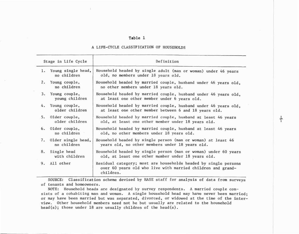
Table 1

A LIFE-CYCLE CLASSIFICATION OF HOUSEHOLDS

Stage in Life Cycle

1. Young single head,no children

2. Young couple,no children

3. Young couple,young children

4. Young couple,older children

5. Older couple,older children

6. Older coupl~,

no children

7. Older single head,no children

8. Single headwith children

9. All other

Definition

Household headed by single adult (man or woman) under 46 yearsold, no members under 18 years old.

Household headed by married couple, husband under 46 years old,no other members under 18 years old.

Household headed by married couple, husband under 46 years old,at least one other member under 6 years old.

Household headed by married couple, husband under 46 years old,at least one other member between 6 and 18 years old.

Household headed by married couple, husband at least 46 yearsold, at least one other member under 18 years old.

Household headed by married couple, husband at least 46 yearsold, no other members under 18 years old.

Household headed by single person (man or woman) at least 46years old, no other members under 18 years old.

Household headed by single person (man or woman) under 60 yearsold, at least one other member under 18 years old.

Residual categ~ry; most are households headed by single personsover 60 years old who live with married children and grand­children.

I~

I

SOURCE: Classification scheme devised by HASE staff for analysis of data from surveysof tenants and homeowners.

NOTE: Household heads are designated by survey respondents. A married couple con­sists of a cohabiting man and woman. A single household head may have never been married;or may have been married but was separated, divorced, or widowed at the time of the inter­view. Other household members need not be but usually are related to the householdhead(s); those under 18 are usually children of the head(s).

-7-

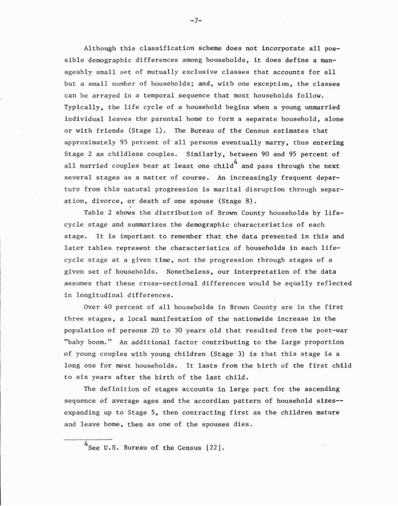
Although this classification scheme does not incorporate all pos­

sible demographic differences among households, it does define a man­

ageably small set of mutually exclusive classes that accounts for all

but a small number of households; and, with one exception, the classes

can be arrayed in a temporal sequence that most households follow.

Typically, the life cycle of a household begins when a young unmarried

individual leaves the parental home to form a separate household, alone

or with friends (Stage 1). The Bureau of the Census estimates that

approximately 95 percent of all persons eventually marry, thus entering

Stage 2 as childless couples. Similarly, between 90 and 95 percent of

all married couples bear at least one child4 and pass through the next

several stages as a matter of course. An increasingly frequent depar­

ture from this natural progression is marital disruption through separ­

ation, divorce, or death of one spouse (Stage 8).

Table 2 shows the distribution of Brown County households by life­

cycle stage and summarizes the demographic characteristics of each

stage. It is important to remember that the data presented in this and

later tables ~epresent the characteristics of households in each life­

cycle stage at a given time, not the progression through stages of a

given set of households. Nonetheless, our interpretation of the data

assumes that these cross-sectional differences would be equally reflected

in longitudinal differences.

Over 40 percent of all households in Brown County are in the first

three stages, a local manifestation of the nationwide increase in the

population of persons 20 to 30 years old that resulted from the post-war

"baby boom." An additional factor contributing to the large proportion

of young couples with young children (Stage 3) is that this stage is a

long one for most households. It lasts from the birth of the first child

to six years after the birth of the last child.

The definition of stages accounts in large part for the ascending

sequence of average ages and the accordian pattern of household sizes-­

expanding up to Stage 5, then contracting first as the children mature

and leave home, then as one of the spouses dies.

4See U.S. Bureau of the Census [22].

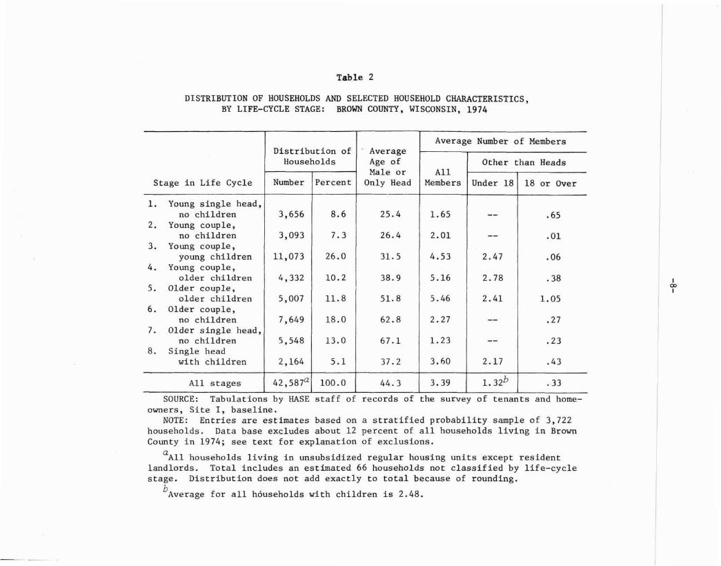
Table 2

DISTRIBUTION OF HOUSEHOLDS AND SELECTED HOUSEHOLD CHARACTERISTICS,BY LIFE-CYCLE STAGE: BROWN COUNTY, WISCONSIN, 1974

Average Number of MembersDistribution of - Average

Households Age of Other than HeadsMale or All

Stage in Life Cycle Number Percent Only Head Members Under 18 18 or Over

1. Young single head,no children 3,656 8.6 25.4 1.65 -- .65

2. Young couple,no children 3,093 7.3 26.4 2.01 -- .01

3. Young couple,young children 11,073 26.0 31. 5 4.53 2.47 .06

4. Young couple,older children 4,332 10.2 38.9 5.16 2.78 .38

5. Older couple,older children 5,007 11.8 51. 8 5.46 2.41 1.05

6. Older couple,no children 7,649 18.0 62.8 2.27 -- .27

7. Older single head,no children 5,548 13.0 67.1 1. 23 -- .23

8. Single headwith children 2,164 5.1 37.2 3.60 2.17 .43

All stages 42,587a 100.0 44.3 3.39 1. 32b .33

SOURCE: Tabulations by RASE staff of records of the survey of tenants and home­owners, Site I, baseline.

NOTE: Entries are estimates based on a stratified probability sample of 3,722households. Data base excludes about 12 percent of all households living in BrownCounty in 1974; see text for explanation of exclusions.

aAll households living in unsubsidized regular housing units except residentlandlords. Total includes an estimated 66 households not classified by life-cyclestage. Distribution does not add exactly to total because of rounding.

bAverage for all households with children is 2.48.

I00I

-9-

The demographic changes which mark the life-cycle progression do

not occur in isolation. Accompanying this progression are changes in

the households' social and economic circumstances that will also affect•housing choices.

The most important changes accompanying the life-cycle progression

occur in labor-force participation by household members and in household

income. Several factors contribute to these changes. Foremost among

them is the general correspondence between the life cycle and the career

development of the male head of the household.

Just as Stage 1 marks the individual's formation of a new house­

hold, it also usually marks his economic independence and the beginning

of regular full-time employment. In this stage, his earnings are

usually low, but they typically increase as he develops occupational

skills and acqui~es' seniority. Eventually, he retires from the labor

force because of age or disability, at which point there is usually a

sudden and sharp drop in household income.

The male head's employment history is, of course, not the only ele­

ment in a household's employment and income profiles. Labor-force

participation by wives and adolescent children is common and contributes

substantially to the earnings of many households.

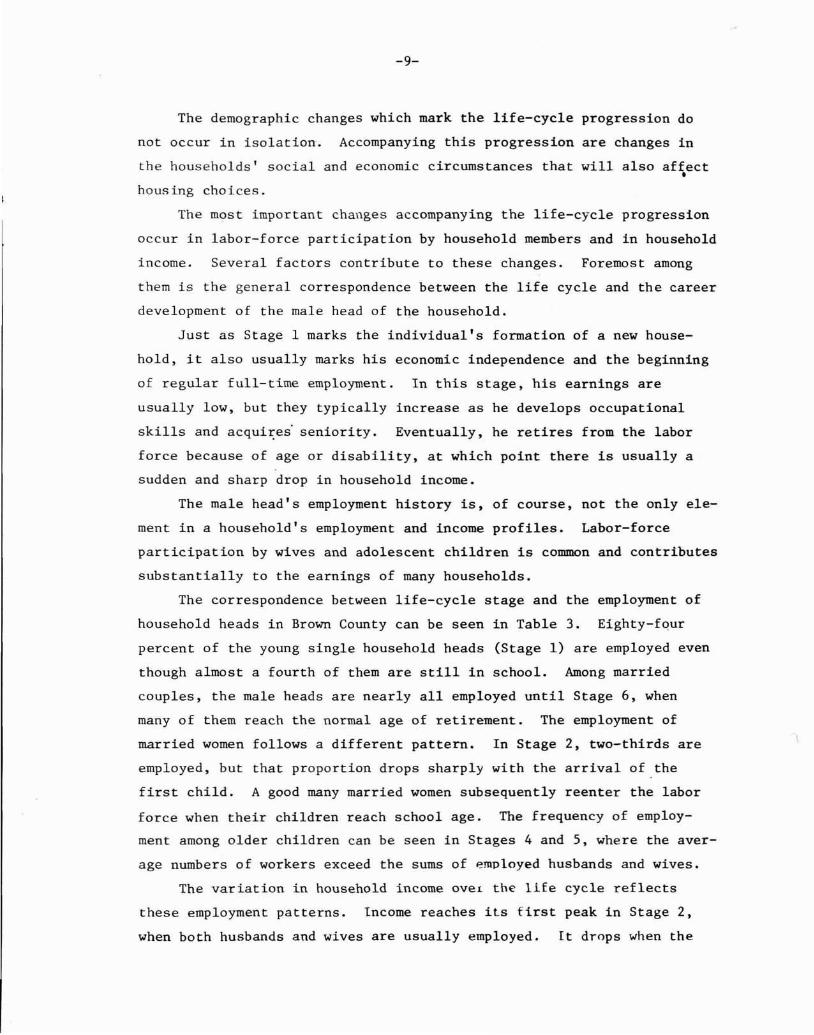
The correspondence between life-cycle stage and the employment of

household heads in Brown County can be seen in Table 3. Eighty-four

percent of the young single household heads (Stage 1) are employed even

though almost a fourth of them are still in school. Among married

couples, the male heads are nearly all employed until Stage 6, when

many of them reach the normal age of retirement. The employment of

married women follows a different pattern. In Stage 2, two-thirds are

employed, but that proportion drops sharply with the arrival of the

first child. A good many married women subsequently reenter the labor

force when their children reach school age. The frequency of employ­

ment among older children can be seen in Stages 4 and 5, where the aver­

age numbers of workers exceed the sums of employed husbands and wives.

The variation in household income over the life cycle reflects

these employment patterns. Income reaches its first peak in Stage 2,

when both husbands and wives are usually employed. It drops when the

Table 3

EMPLOYMENT AND INCOME CHARACTERISTICS OF HOUSEHOLDS. BY LIFE-CYCLE STAGE:BROWN COUNTY. WISCONSIN, 1974

Percentage of Households with:

Male or Only HeadaAverage Median

Wife No Members Number of Income ($)Stage in Life Cycle In School Employed Employed Employed Workers in 1973

l. Young single head,no children 23.3 83. 7 (b) 7.1 1.40 7,564

2. Young couple.no children 11.6 90.9 67.2 1.8 1. 59 13.433

3. Young couple.young children 4.5 95.6 30.6 2.4 1. 30 12.656

4. Young couple.older children 1.3 97.9 48.6 1.1 1. 74 14.593

S. Older couple.older children .9 92.3 34.2 1.2 2.15 17,549

6. Older couple,no children -- 61. 2 27.1 29.6 1.07 10.965

7. Older single head.no children -- 35.3 (b) 57.5 .51 4.697

8. Single head,with children 8.4 56.4 (b) 35.6 .75 5,704

All stages 4.7 77.9 36.Sc 16.3 1. 30 11,988

SOURCE: Tabulations by HASE staff of records of the survey of tenants and homeowners.Site I. baseline.

NOTE: Employment entries are estimates based on a stratified probability sample of3.722 households; income entries are based on a smaller sample of 3,223 households report­ing complete income information. Data base excludes about 12 percent of all householdsliving in Brown County in 1974; see text for explanation of exclusions.

aHousehold heads in school may also be employed.

bNot applicable.

c Base for percentage includes only households headed by a married couple.

I.....oI

-11-

wives leave the labor force to care for their young children and then

rises as mothers return to the labor force and both husbands and wives

acquire skills and seniority in their jobs. Household income reaches

its peak in Stage 5, when the number of workers in the household is

also at its peak, often including the husband, the wife, and one or

more of the older children. As the children leave home and the heads

retire from the labor force (Stages 6 and 7), household income drops

sharply.

LIFE-CYCLE STAGES AND HOUSING CONSUMPTION

These data suggest that there should be a particularly strong re­

lationship between housing consumption and progression through the life

cycle. Movement through life-cycle stages brings characteristic changes

in the size and composition of households and, consequently, in their

housing requirements. The concomitant changes in the household's social

and economic characteristics, particularly the changes in income,

affect the household's ability to adjust its consumption accordingly.

In general, these two kinds of changes complement each other. However,

this is not always the case. For example, between Stages 2 and 3, aver­

age household size increases by 2.5 persons but household income de­

creases. The increased space requirements of these larger households,

along with their increased requirements for food and clothing, must

often be met from the same or a smaller budget, forcing many households

to compromise in their housing choices.

In later stages, household consumption needs and the means to sat­

isfy them are better balanced. Peak household size occurs in Stage 5,

which is also the stage of peak household income. When income begins

to drop sharply (Stages 6 and 7), the number of persons to be supported

by that income also decreases sharply.

Tenure and Type of Housing Unit

Although most single-family houses are owner-occupied and most

apartments in multiple dwellings are renter-occupied, it is important

to distinguish tenure and type of housing as separate dimensions of

housing choice. As households move through the life cycle, there are

-12-

characteristic shifts in tenure from rental to ownership and back to

rental. Although owners nearly always live in single-family houses,

there are also characteristic changes in the type of housing selected

by renters at different stages of the life cycle.

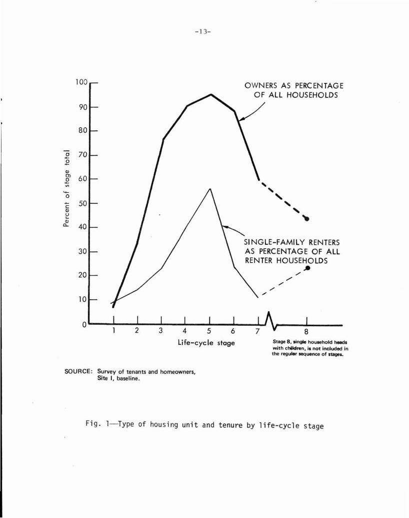
Figure 1 displays the main features of these two choices in rela­

tion to life-cycle stages. Less than 7 percent of all young single

household heads are homeowners; the others rent their homes, and 90

percent of these renters live in apartments. This pattern is, of

course, consistent with the relatively small space requirements, the

relatively low incomes, and the considerable occupational and demo­

graphic instability of these households. The incidence of homeowner­

ship rises sharply thereafter, reaching 95 percent in Stage 5. Nearly

all of these homeowners occupy single-family houses. Among renters in

the middle of the life cycle there is also a decided shift from apart­

ments to single-family houses; by Stage 5, nearly 60 percent of the

renters and 98 percent of all households live in single-family houses.

In the later stages of the life cycle, when the children have

left home and finally when one of the spouses dies, the incidence of

both ownership and of renters in single-family houses declines. In

Stage 7, only 45 percent of all households own their homes and only

10 percent of all renters live in single-family houses.

When the patterns shown in the figure are considered in conjunc­

tion with the data on household characteristics by life-cycle stage,

two important ideas emerge. First, although nearly everyone in Brown

County lives in a single-family house during the peak years of house­

hold size and income, few spend all their adult years in such a resi-5dence. Second, renters and homeowners in the same life-cycle stages

appear to be less distinguished by different housing preferences than

by different resources for satisfying those preferences. Thus, it is

likely that more renters in the middle of the life cycle would prefer

single-family homes to apartments but cannot afford them.

5This pattern does not apply equally to all local housing markets.Both the size of the market (Carliner [3]) and the racial compositionof the population are likely to affect life-cycle patterns of homeowner­ship.

100

90

80

0 70....0....Q)

OJ 600....\I)....0

.... 50cQ)

u....Q)

c.. 40

30

20

10

0

-]3-

OWNERS AS PERCENTAGEOF ALL HOUSEHOLDS

",,"" ~

SI NGLE-FAMILY RENTERSAS PERCENTAGE OF ALLRENTER HOUSEHOLDS..

./,/

./

life-cycle stage

SOURCE: Survey of tenants and homeowners,Site I, baseline.

Stage 8, single household heKIswith children, is not included inthe regular sequence of stages.

Fig. l--Type of housing unit and tenure by life-cycle stage

-14-

The preference for single-family homes characteristic of the middle

stages of the life cycle undoubtedly reflects the importance of indoor

and outdoor space to households with children. The role of income as

a constraint on this preference is less straightforward because it tends

to vary over life-cycle stages in parallel with the number of children

in the household. However, there is considerable variation in income

among households within a given stage, which is likely to affect the6choice both of housing type and of tenure.

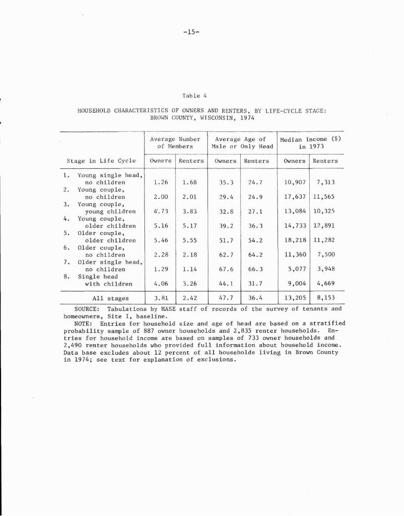
The data shown in Table 4 indicate that with only one exception,

Stage 3, renters and owners in the same life-cycle stage have house­

holds of approximately the same size, so that both groups of households

should experience similar pressures for living space. A notable dif­

ference between owners and renters is in their ages. In the earlier

stages of the life cycle, household heads who are owners tend to be

older than those who are renters; in the older stages, owners tend to

be younger than renters. Thus, at each stage, owners are closer than

renters to their peak lifetime earnings.

These differences in age are one factor accounting for the pattern

of income differences between owner and renter households at each life­

cycle stage, also shown in Table 4. This pattern indicates that owners

are more prosperous than renters in all life-cycle stages, and especi­

ally so in Stages 2, 5, and 6. In the earlier stage, they are there­

fore better able to accumulate a downpayment on a house before the wife

leaves the labor force to have children. In the later stages, the more

prosperous homeowners are less often impelled to economize by moving

to smaller homes after their children have left the household.

Size of Housing Unit

Housing is a complex commodity, and differences in tenure and type

of units by no means encompass the household's range of choices. The

decision to live in a single-family house rather than an apartment will

be based in part on such other factors as unit size and cost. We have

6An appendix to this paper reports on a regression model that helpsto sort out tpe independent relationships of housing tenure to life­cycle stages on the one hand and to income on the other hand.

-15-

Table 4

HOUSEHOLD CHARACTERISTICS OF OWNERS AND RENTERS, BY LIFE-CYCLE STAGE:BROWN COUNTY, WISCONSIN, 1974

Average Number Average Age of Median Income ($)of Members Male or Only Head in 1973

-Stage in Life Cycle Owners Renters Owners Renters Owners Renters

l. Young single head,no children 1. 26 1. 68 35.3 24.7 10,907 7,313

2. Young couple,no children 2.00 2.01 29.4 24.9 17,637 11,565

3. Young couple,young children 4·.73 3.83 32.8 27.1 13,084 10,32')

4. Young couple,I

older children 5.16 5.17 39.2 36.3 14,733 17. ,8915. Older couple,

older children 5.46 5.55 51. 7 54.2 18,218 11,2826. Older couple,

no children 2.28 2.18 62.7 64.2 11,360 7,5007. Older single head,

no children 1. 29 1.14 67.6 66.3 5,077 3,9488. Single head

with children 4.06 3.26 44.1 31. 7 9,004 4,669

All stages 3.Rl 2.42 47.7 36.4 13,205 8,153

SOURCE: Tabulations by HASE staff of records of the survey of tenants andhomeowners, Site I, baseline.

NOTE: Entries for household size and age of head are based on a stratifiedprobability sample of 887 owner households and 2,835 renter households. En­tries for household income are based on samples of 733 owner households and2,490 renter households who provided full information about household income.Data base excludes about 12 percent of all households living in Brown Countyin 1974; see text for explanation of exclusions.

-16-

already described single-family houses as more spacious than apart­

ments in multiple dwellings. This characterization is appropriate

both in the narrow sense of number of rooms and in the broader sense

of insulation from neighbors and access to private outdoor space.

In Brown County, the average number of rooms in owner-occupied

single-family houses is 6.02; in renter-occupied single-family houses,

5.22; in small (2-4 unit) multiple dwellings, 4.17 rooms; and in large

(5+ units) multiple dwellings, 3.43 rooms. While we do not have such

exact information about the sizes of yards, it. is clear that those who

live in multiple dwellings have less access to private outdoor space.

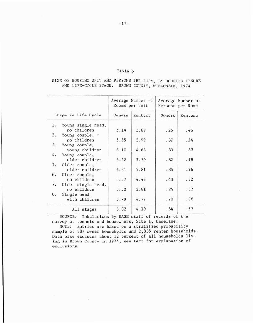
The variation in average unit size and persons per room by life­

cycle stage for owners and renters is reported in Table 5. Households

in both tenure classes tend to increase their space consumption as

household size increases (Stages 1 to 5), then to reduce it as house­

hold size shrinks in Stages 6 and 7. However, owners have larger units

than renters at every life-cycle stage. These differences are largest

(about 1.7 rooms) among young childless couples (Stage 2) and among

older single-headed households (Stage 7); they are smallest (0.8 rooms)

for older couples with children (Stages 5 and 6). This pattern in aver­

age unit size, along with the accompanying person-per-room ratios,

suggests that childless couples purchase homes larger tha~ they need

at the time in anticipation of future growth in household size; and

that older households are reluctant to move to smaller homes after the

departure of their children.

Since household sizes for renters and owners at each stage are

approximately the same, renters appear to be consistently more crowded

than owners. Nonetheless, there is no stage in which renter households

in Brown County average more than one person per room; indeed, a smaller

proportion of renters than owners (4 percent vs. 8 percent) exceed that

standard. Thus it appears that by moving from one unit to another as

household size changes, renter households are able to avoid overcrowding.

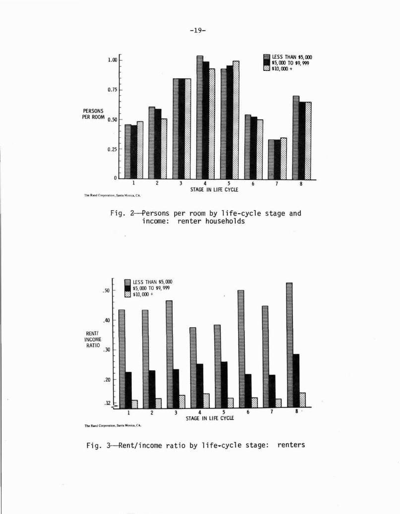
Because income also varies by life-cycle stage, we examine the

space consumption of Brown County households by life-cycle stage and

income level in Fig. 2. This comparison is limited to renter households

because they exhibit greater adaptability in their space consumption.

-17-

Table 5

SIZE OF HOUSING UNIT AND PERSONS PER ROOH, BY HOUSING TENUREAND LIFE-CYCLE STAGE: BROWN COUNTY, WISCONSIN, 1974

Average Number of Average Number ofRooms per Unit Persons per Room

Stage in Life Cycle Owners Renters Owners Renters

l. Young single head,no children 5.14 3.69 .25 .46

2. Young couple,no children 5.65 3.q9 .37 .54

3. Young couple,young children 6.10 4.66 .80 .83

4. Young couple,older children 6.52 5.39 .82 .98

5. Older couple,older children 6.61 5.81 .84 .96

6. Older couple,no children 5.57 4.42 .43 .52

7. Older single head,no children 5.52 3.81 .24 .32

8. Single headwith children 5.79 4.77 .70 .68

All stages 6.02 4.19 .64 .57

SOURCE: Tabulations by RASE staff of records of thesurvey of tenants and homeowners, Site 1., baseline.

NOTE: Entries are based on a stratified probabilitysample of 887 owner households and 2,835 renter households.Data base excludes about 12 percent of all households liv­ing in Brown County in 1974; see text for explanation ofexclusions.

-18-

The figure shows the same pattern of space adjustment across life­

cycle stages at each income level; within life-cycle stages, space

consumption is unaffected by income. As we shall see, the more pros­

perous renters within each life-cycle stage do spend more for housing,

but the desire for more space does not appear to be the motivating

factor.

7Income and Housing Expenditures: Renters

A comparison of the average monthly gross rent of renter house­

holds paying full rent by life-cycle stage and income indicates an

expectable expenditure pattern. Within each income class, expenditures

increase from the early to the middle stages of the life cycle and

then decline in the later stages. This pattern reflects the changing

space requirements of households over these stages. For households

within each life-cycle stage, expenditures have a general tendency to

increase with income, but the amounts of increase are irregular.

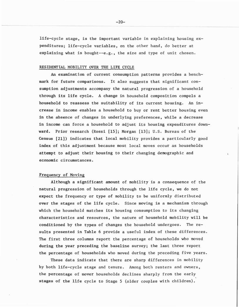
A clearer picture of the relationship between housing expenditures

and income can be seen in Fig. 3, in which the average rent/income ratios

for individual households are compared. Although the differences in

relative expenditures between stages generally disappear, the average

ratios drop sharply as income increases. Households in the lowest in­

come bracket spend almost twice the proportion of their incomes on

housing as do those in the middle bracket and over three times the pro­

portion as do those in the upper bracket. The pattern reflected in

this figure contrasts sharply with the comparison of person-per-room

ratios pictured in Fig. 2.. This contrast suggests that income, not

7Estimating housing expenditures for homeowners is considerablymore difficult than it is for renters. While gross rent is a rela­tively accurate measure of the renter's total housing expenditures,a comparable measure for owners must include not only debt service,utility expenditures, taxes, and insurance but also the imputed valueof the homeowner's time spent on maintenance and repair, as well as theopportunity costs entailed in buying a home rather than investing equiv­alent savings in some other way. Since we are still working on theseaccounting problems, we will not present any tabulations of homeownerhousing expenses here.

I LISS THAN $5, em... $5, em TO $9, 999.:.;. no, em +

1.00

0.75

PERSONSPER ROOM 0.50

0.25

o

The Rand Corpor'ltOn. Santi Monica. CA.

2

-19-

345STAGE IN LIFE CYCLI

6 7 8

.50

Fig. 2--Persons per room by life-cycle stage andincome: renter households

I LISS THAN $5, em$5, em TO $9, 999

;::: $10, em +

.40

RENTIINCOMERATIO

.30

.20

.12

2 3 4 5STAGE IN LIFE CYCLI

The Rand Corporation, Santi Monka. CA.

Fig. 3--Rent/income ratio by life.cycle stage: renters

-20-

life-cycle stage~ is the important variable in explaining housing ex­

penditures; life-cycle variables~ on the other hand, do better at

explaining what is bought--e.g., the size and type of unit chosen.

RESIDENTIAL MOBILITY OVER THE LIFE CYCLE

An examination of current consumption patterns provides a bench­

mark for future comparisons. It also suggests that significant con­

sumption adjustments accompany the natural progression of a household

through its life cycle. A change in household composition compels a

household to reassess the suitability of its current housing. An in­

crease in income enables a household to buy or rent better housing even

in the absence of changes in underlying preferences~ while a decrease

in income can force a household to adjust its housing expenditures down­

ward. Prior research (Rossi [15]; Morgan [13]; u.s. Bureau of the

Census [21]) indicates that local mobility provides a particularly good

index of this adjustment because most local moves occur as households

attempt to adjust their housing to their changing demographic and

economic circumstances.

Frequency of Moving

Although a significant amount of mobility is a consequence of the

natural progression of households through the life cycle~ we do not

expect the frequency or type of mobility to be uniformly distributed

over the stages of the life cycle. Since moving is a mechanism through

which the household matches its housing consumption to its changing

characteristics and resources~ the nature of household mobility will be

conditioned by the types of changes the household undergoes. The re­

sults presented in Table 6 provide a useful index of these differences.

The first three columns report the percentage of households who moved

during the year preceding the baseline survey; the last three report

the percentage of households who moved during the preceding five years.

These data indicate that there are sharp differences in mobility

by both life-cycle stage and tenure. Among both renters and owners,

the percentage of mover households declines sharply from the early

stages of the life cycle to Stage 5 (older couples with children).

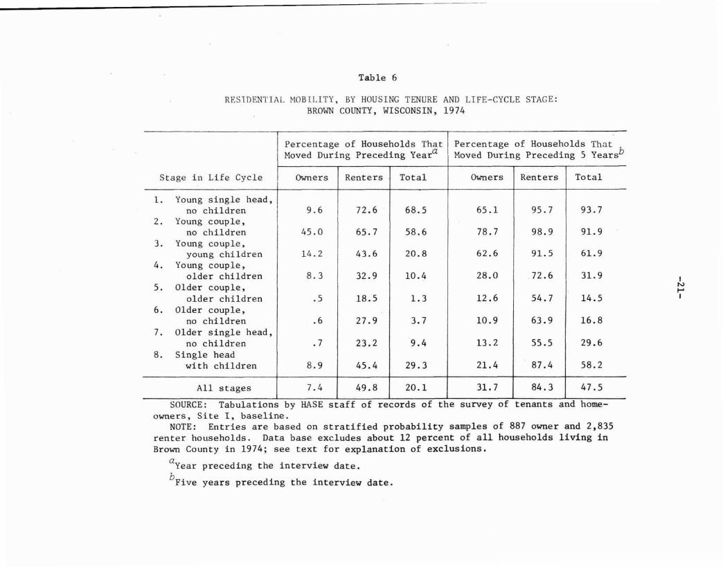
Table 6

RESIDENtIAL MOBILITY, BY HOUSING TENURE AND LIFE-CYCLE STAGE:BROWN COUNTY, WISCONSIN, 1974

Percentage of Households That Percentage of Households ThatMoved During Preceding Yeara Moved During Preceding 5 Yearsb

Stage in Life Cycle Owners Renters Total Owners Renters Total

l. Young single head,no children

I9.6 72.6 68.5 65.1 95.7 93.7

2. Young couple,no children 45.0 65.7 58.6 78.7 98.9 91. 9

3. Young couple,young children 14.2 43.6 20.8 62.6 91. 5 61.9

4. Young couple,older children 8.3 32.9 10.4 28.0 .72.6 31. 9

5. Older couple,older children .5 18.5 1.3 12.6 54.7 14.5

6. Older couple,no children .6 27.9 3.7 10.9 63.9 16.8

7. Older single head,no children .7 23.2 9.4 13.2 55.5 29.6

8. Single headwith children 8.9 45.4 29.3 21.4 87.4 58.2

All stages 7.4 49.8 20.1 31. 7 84.3 47.5

SOURCE: Tabulations by HASE staff of records of the survey of tenants and home­owners, Site I, baseline.

NOTE: Entries are based on stratified probability samples of 887 owner and 2,835renter households. Data base excludes about 12 percent of all households living inBrown County in 1974; see text for explanation of exclusions.

a Year preceding the interview date.

bFive years preceding the interview date.

IN....J

-22-

This pattern undoubtedly reflects- the considerable instability during. .

early stages of the life cycle of household size and composition on

the one hand and of employment and income on the other. As childbear­

ing is completed and career patterns become more definite, both the

household's housing needs and the resources available to satisfy those

needs stabilize. The slight in~rease in the mobility of renter house­

holds in Stages 6 and 7 probably reflects an adjustment in consumption

due to the declining household sizes and incomes common to these stages.

Mobility and Housing Tenure

Just as striking as the differences in mobility over the life cycle

are the differences between renters and owners. At every life-cycle

stage, renters are significantly more likely to be movers than owners.

Several factors contribute to this difference. First, as the results

in Table 5 indicated, owner-occupied homes are significantly larger than

rented units, so that owner households have more flexibility in adapting

to changes in household size. Second, the decision to purchase a home

is in a real sense a manifestation of the household's stability. Buy­

ing a house is the single largest investment most households ever make.

This decision is not likely to be made until the household's income is

relatively stable and unless the household is committed to remaining in

the residence for some time. Research by Shelton [17], for example,

indicates that owning is less expensive than renting only if the period

of ownership exceeds four years. Third, the circumstances of homeowner­

ship and the expenses associated with moving are likely to reinforce the

household's stability, so that opportunities that might have appealed to

them as renters are foregone as homeowners.

The household's satisfaction with its move and the probability of

its moving again in the near future will depend on the type of move that

it makes. In Table 7 we examine the characteristics of moves over the

life-cycle.stages in terms of the tenure of the prior and current units.

These data are limited to the 80 percent of all households who moved at

least once in the five years preceding the survey and whose last prior

residence was also in Brown County. Detailed data on prior residences

were collected only for these local moves.

--

Table 7

CHANGES IN HOUSING TENURE FOR LOCAL MOVERS, BY LIFE-CYCLE STAGE:BROWN COUNTY, WISCONSIN, 1974

Percentage Distributions of Households by Former and Current Tenure

Former Owners Former Renters New HouseholdsP Numberby Current Tenure by Current Tenure by Current Tenure of Last

LocalStage in Life Cycle Owner Renter Owner Renter Owner Renter Total Moves

1. Young s~ngle head,no children -- 5.2 3.6 69.4 1.6 20.3 100.0 2,591

2. Young couple,no children 5.3 1.0 24.8 41.8 5.5 21. 5 100.0 2,287

3. Young couple,young children 14.1 .6 55.0 24.3 1.8 4.2 100.0 6,129

4. Young couple,older children 39.2 1.9 36.5 21. 5 -- .9 100.0 850

5. Older couple,older children 80.6 2.5 -- 16.3 .5 -- 100.0 589

6. Older couple,no children. 58.1 9.1 6.1 24.6 2.1 -- 100.0 1,085

7. Older single head,no children 23.9 27.oj 4.8 41.4 -- 2.0 100.0 1,412

8. Single head,with children 3.8 9.6 12.3 66.7 -- 7.6 100.0 1,136

All stages 17.6 5.1 28.7 38.1 1.9 8.7 100.0 16,079

SOURCE: Tabulations by RASE staff of records of the survey of tenants and homeowners, Site I,baseline.

NOTE: Entries compare housing tenure before and after respondent's last local move. Distributionsare based on a stratified probability sample of 2,039 households whose last move occurred during thefive years preceding the interview and who moved within Brown County. Data base excludes about 12 per­cent of all households in Brown County in 1974; see text for explanation of exclusions.

aprior to last move, respondent was not a household head.

Itv\..VI

-24-

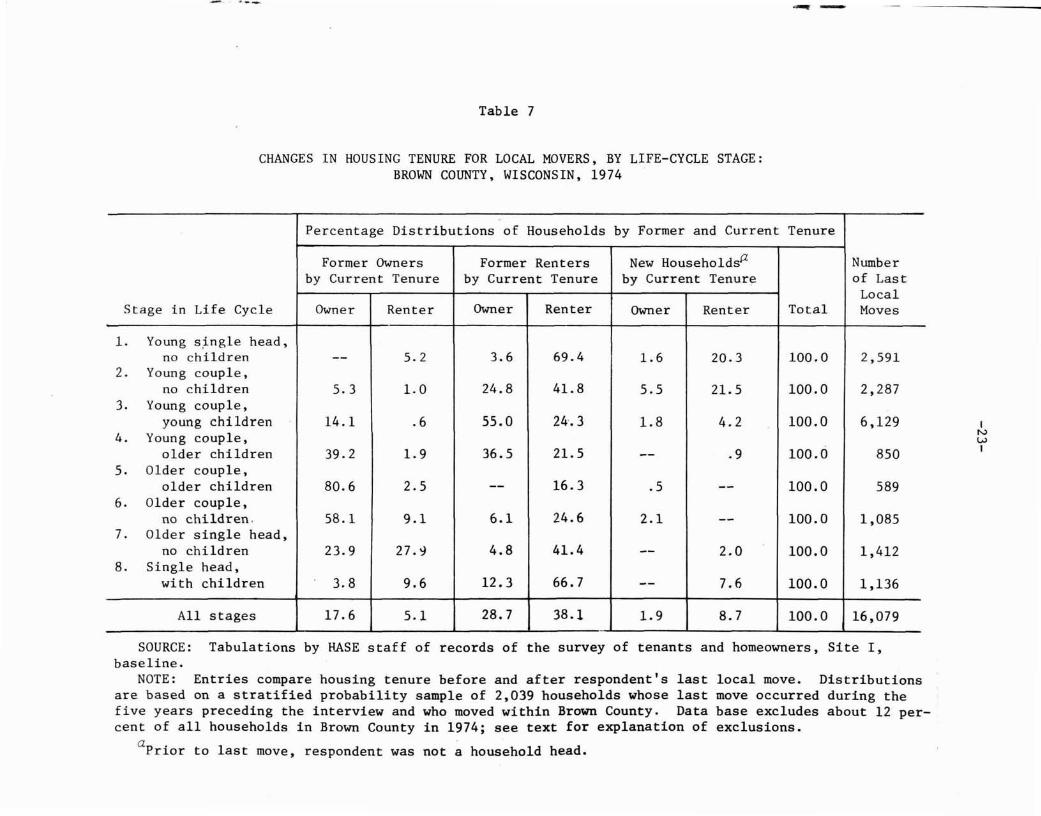
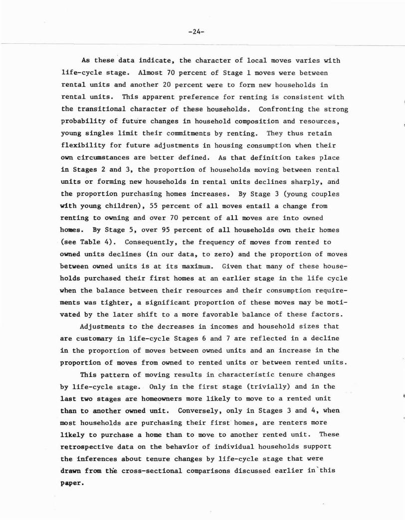
As these data indicate, the character of local moves varies with

life-cycle stage. Almost 70 percent of Stage 1 moves were between

rental units and another 20 percent were to form new households in

rental units. This apparent preference for renting is consistent with

the transitional character of these households. Confronting the strong

probability of future changes in household composition and resources,

young singles limit their commitments by renting. They thus retain

flexibility for future adjustments in housing consumption when their

own circumstances are better defined. As that definition takes place

in Stages 2 and 3, the proportion of households moving between rental

units or forming new households in rental units declines sharply, arid

the proportion purchasing homes increases. By Stage 3 (young couples

with young children), 55 percent of all moves entail a change from

renting to owning and over 70 percent of all moves are into owned

homes. By Stage 5, over 95 percent of all households own their homes

(see Table 4). Consequently, the frequency of moves from rented to

owned units declines (in our data, to zero) and the proportion of moves

between owned units is at its maximum. Given that many of these house­

holds purchased their first homes at an earlier stage in the life cycle

when the balance between their resources and their consumption require­

ments was tighter, a significant proportion of these moves may be moti­

vated by the later shift to a more favorable balance of these factors.

Adjustments to the decreases in incomes and household sizes that

are customary in life-cycle Stages 6 and 7 are reflected in a decline

in the proportion of moves between owned units and an increase in the

proportion of moves from owned to rented units or between rented units.

This pattern of moving results in characteristic tenure changes

by life-cycle stage.· Only in the first stage (trivially) and in the

last two stages are homeowners more likely to move to a rented unit

than to another owned unit. Conversely, only in Stages 3 and 4, when

most households are purchasing their first-homes, are renters more

likely to purchase a home than to move to another rented unit. These

retrospective data on the behavior of individual households support

the inferences about tenure changes by life-cycle stage that were

drawn from tne cross-sectional comparisons discussed earlier in'this

paper.

-25-

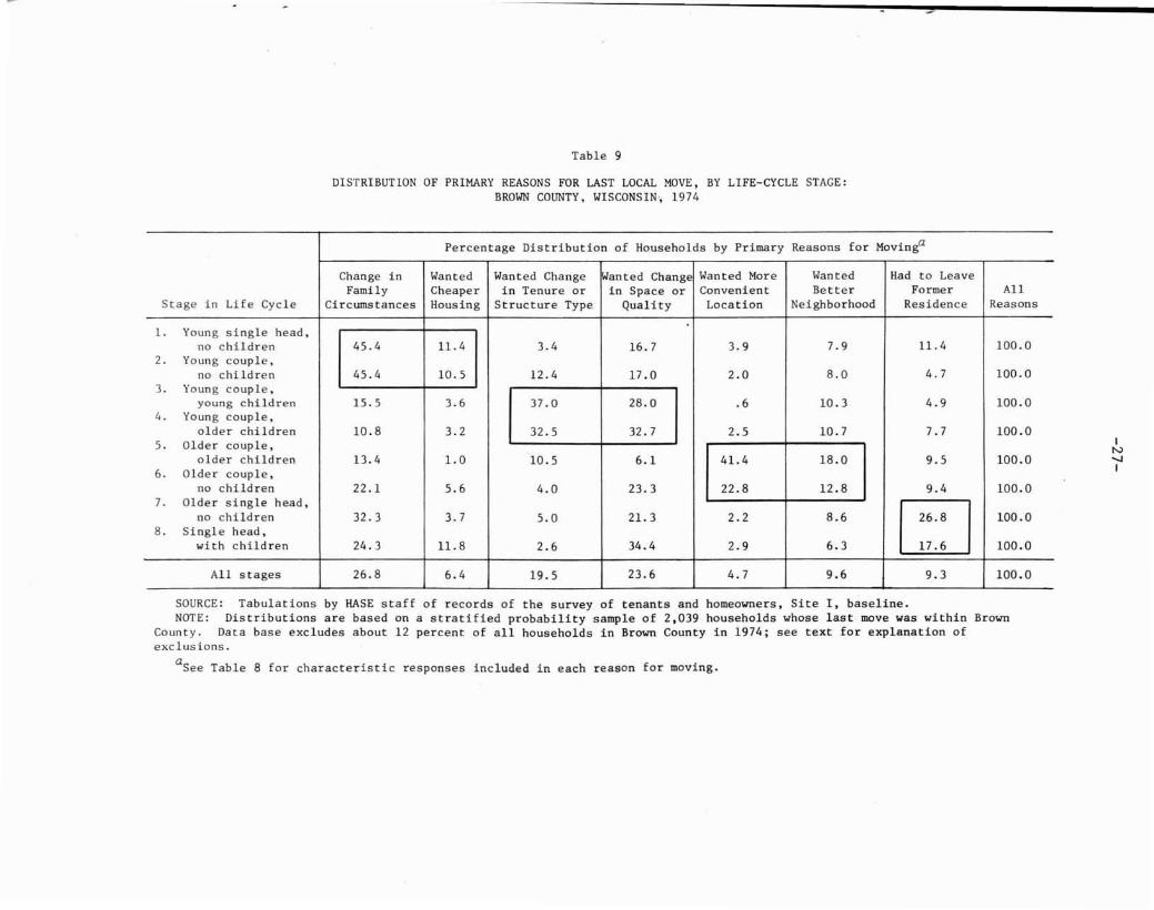
Reasons for Moving

The life-cycle differences in movers' housing choices undoubtedly

reflect the different circumstances that prompt moves in each lif~­

cycle stage. Comparing the primary reasons for moving reported by

households in each stage should therefore give us additional insight

into the factors at work. This is done in Tables 8 and 9.

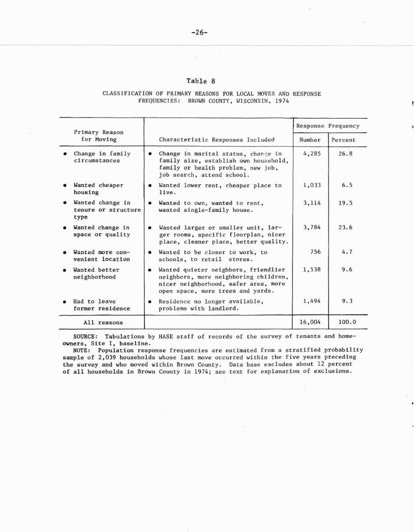
Table 8 classifies recent movers' reported motivations into seven

primary reasons for moving. Coding interview responses of this type

is difficult, because different respondents may express essentially

the same motivation quite differently. For example, following the

birth of a couple's first child, they may decide that they need a home

with a second bedroom; the respondent may describe the decision as

prompted by changes in family circumstances or by a desire for more

space. Our coding' was guided by the respondent's own emphasis, and

the results shown in Table 9 suggest that this was a valid criterion.

Overall, a fourth of all movers mentioned some change in family

circumstances as their primary reason for moving (Table 8). Over 40

percent mentioned a desire for homeownership, a single-family house,

or more space or better quality as the primary reason. It should not

be surprising in a small metropolitan area with such a homogeneous

population that few respondents cited location (5 percent) or neigh­

borhood characteristics (10 percent) as the motive for their moves.8

Involuntary moves accounted for about 9 percent of the total, and the

explicit desire for cheaper housing was reported in fewer than 7 per­

cent of all cases.

The ordering of primary reasons in Table 8 was chosen because it

corresponds fairly well with the shifts in emphasis over the household

life cycle. This is demonstrated in Table 9. Note there that the

greatest emphasis on changes in family circumstances comes during the

first two stages of the life cycle; these are also the stages in which

8However, several other studies, some of which were conducted inlarger urban areas, also find that location and neighborhood charac­teristics are subordinate to changes in family circumstances as reasonsfor moving (Rossi [15]; Greenbie [8]; Gans [6]).

-26-

Table 8

CLASSIFICATION OF PRIMARY REASONS FOR LOCAL MOVES AND RESPONSEFREQUENCIES: BROWN COUNTY, WISCONSIN, 1974

Response FrequencyPrimary Reason

for Moving

• Change in familycircumstances

• Wanted cheaperhousing

• Wanted change intenure or structuretype

• Wanted change inspace or quality

• Wanted more con­venient location

• Wanted betterneighborhood

• Had to leaveformer residence

All reasons

Characteristic Responses Included

• Change in marital status, chan 0e infamily size, establish own household,family or health problem, new job,job search, attend school.

• Wanted lower rent, cheaper place tolive.

• Wanted to own, wanted to rent,wanted single-family house.

• Wanted larger or smaller unit, lar­ger rooms, specific floorplan, nicerplace, cleaner place, better quality.

• Wanted to be closer to work, toschools, to retail stores.

• Wanted quieter neighbors, friendlierneighbors, more neighboring children,nicer neighborhood, safer area, moreopen space, more trees and yards.

• Residence no longer available,problems with landlord.

Number

4,285

1,033

3,114

3,784

756

1,538

1,494

16,004

Percent

26.8

6.5

19.5

23.6

4.7

9.6

9.3

100.0

SOURCE: Tabulations by HASE staff of records of the survey of tenants and home­owners, Site I, baseline.

NOTE: Population response frequencies are estimated from a stratified probabilitysample of 2,039 households whose last move occurred within the five years precedingthe survey and who moved within Brown County. Data base excludes about 12 percentof all households in Brown County in 1974; see text for explanation of exclusions.

::s

Table 9

DISTRIBUTION OF PRIMARY REASONS FOR LAST LOCAL MOVE, BY LIFE-CYCLE STAGE:BROWN COUNTY, WISCONSIN, 1974

Percentage Distribution of Households by Primary Reasons for Movinga

Change in Wanted Wanted Change Wanted Change Wanted More Wanted Had to LeaveFamily Cheaper in Tenure or in Space or Convenient Better Former All

Stage in Life Cycle Circumstances Housing Structure Type Quality Location Neighborhood Residence Reasons

1. Young single head,no children 45.4 11. 4 3.4 16.7 3.9 7.9 11.4 100.0

2. Young couple,no children 45.4 10.5 12.4 17.0 2.0 8.0 4.7 100.0

3. Young couple,young children 15.5 3.6 37.0 28.0 .6 10.3 4.9 100.0

4. Young couple,older children 10.8 3.2 32.5 32.7 2.5 10.7 7.7 100.0

5. Older couple,older children 13.4 1.0 10.5 6.1 41. 4 18.0 9.5 100.0

6. Older couple,no children 22.1 5.6 4.0 23.3 22.8 12.8 9.4 100.0

7. Older single head,no children 32.3 3.7 5.0 21. 3 2.2 8.6 c:J 100.0

8. Single head,with children 24.3 11.8 2.6 34.4 2.9 6.3 17.6 100.0

All stages 26.8 6.4 19.5 23.6 4.7 9.6 9.3 100.0

SOURCE: Tabulations by HASE staff of records of the survey of tenants and homeowners, Site I, baseline.NOTE: Distributions are based on a stratified probability sample of 2,039 households whose last move was within Brown

County. Data base excludes about 12 percent of all households in Brown County in 1974; see text for explanation ofexclusions.

a See Table 8 for characteristic responses included in each reason for moving.

IN......I

-28-

housing cost is the most salient consideration in decisions to move.

During Stages 3 and 4, the emphasis shifts to tenure, type of structure,

space, and quality.

During Stage 5, location suddenly emerges as the major considera­

tion and neighborhood characteristics increase in importance. During

Stages 6 and 7, the variety of frequently cited reasons increases to

include changes in family circumstances, change in space or quality,

location, and neighborhood characteristics. In Stage 7, involuntary

moves are prominent for the first time, accounting for over a fourth

of the total.

For disrupted households (Stage 8) outside the regular sequence

of stages, the desire for change in space or quality is the leading

reason for moving, but two other reasons--changes in family circum­

stances and involuntary moves--are also prominent.

It should not be surprising that changes in household circum­

stances are so frequently cited by households in Stages I and 2 of

the life cycle: These households were mostly formed by ~ersons leav­

ing the~r parental homes or getting married. Among young couples with

children, family circumstances are less subject to drastic change, but

the housing choice made in Stage 2 is increasingly inadequate for the

growing, child-centered family. Hence the great emphasis on homeowner­

ship, single-family houses, more space, or better quality, which were

cited as primary reasons for moving by nearly two-thirds of the house­

holds in Stages 3 and 4.

The sudden emphasis on convenience of location and neighborhood

quality that occurs in Stage 5 probably reflects changes both in house­

hold characteristics and in the neighborhoods chosen at earlier stages.

Ninety-five percent of the couples in Stage 5 are homeowners (see Fig.

1) and only 13 percent had moved in the five years preceding the survey

(see Table 8). Their children are older and are beginning to leave

home; the parents may well begin to think more about their own conven­

ience. In a growing urban area, fringe development alters the relative

positions of older neighborhoods in the overall scheme of land use and

traffic patterns. The characters of neighborhoods also change as their

residents age or move and are replaced by new households.

-29-

These factors should continue to be important for households in

Stage 6, but added to them are the sharp decreases in both household

size and income that are characteristic of this stage. Hence the in­

creased emphasis found here on changes in family circumstances and

considerations of space and quality. Following the death of one spouse

(Stage 7), the survivor is likely to be either physically or financi­

ally unable to maintain a single-family home, so involuntary moves are

often reported.

Locational Preference of Movers

Although neither convenience of location nor neighborhood charac­

teristics are prominent in our respondents' articulated reasons for

moving, it does not follow that we should expect random movement within

Brown County. First, th~ decision to move and the choice of a new

residence are not necessarily determined by the same factors (Butler

[2]). Indeed, Greenbie indicates that although few households in his

study cited neighborhood factors as their primary reason for moving, a

majority cited improved surroundings as the most important result of

their moves. Second, in most communities, similar kinds of housing

tend to cluster in neighborhoods, so that those who seek the same kinds

of housing tend to look in the same places.

Neighborhood distinctions within Brown County are minimal. Al­

though areas the size of census tracts can be distinguished by differ­

ent central tendencies in either their housing characteristics or their

population characteristics, the central tendencies themselves are, with

some notable exceptions, weak. But the county does exhibit the common

pattern of declining residential density and more recent residential

development as one moves from the center of Green Bay outward.

To test for differences in locational preferences by life-cycle

stage, we divided the county into roughly concentric rings, following

the tradition of urban sociological analysis (Burgess [1]; Schnore

[16]). We constructed the rings by geographic aggregation of the 108

small neighborhoods into whieh we have divided the county. The divi­

sions correspond generally to the inner and outer portions of the city

of Green Bay, a suburban belt, and the rural remainder of the county.

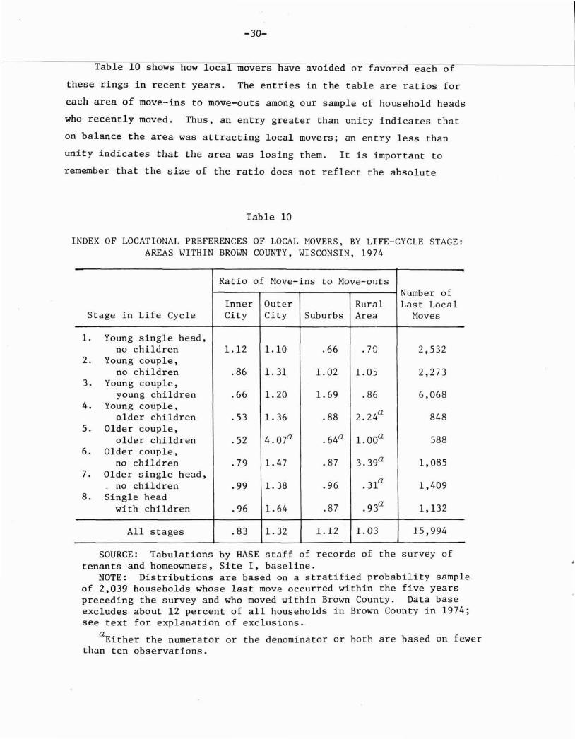
-30-

Table 10 shows how local movers have avoided or favored each of

these rings in recent years. The entries in the table are ratios for

each area of move-ins to move-outs among our sample of household heads

who recently moved. Thus, an entry greater than unity indicates that

on balance the area was attracting local movers; an entry less than

unity indicates that the area was losing them. It is important to

remember that the size of the ratio does not reflect the absolute

Table 10

INDEX OF LOCATIONAL PREFERENCES OF LOCAL MOVERS, BY LIFE-CYCLE STAGE:AREAS WITHIN BROWN COUNTY, WISCONSIN, 1974

Ratio of Move-ins to Move-outsNumber of

Inner Outer Rural Last LocalStage in Life Cycle City City Suburbs Area Moves

1. Young single head,no children 1.12 1.10 .66 .7Q 2,532

2. Young couple,no children .86 1. 31 1. 02 1.05 2,273

3. Young couple,young children .66 1. 20 1. 69 .86 6,068

4. Young couple,older children .53 1. 36 .88 2.24a 848

5. Older couple,older children .52 4. 07a .64a 1.00a 588

6. Older couple,no children .79 1. 47 .87 3.39a 1,085

7. Older single head,- no children .99 1. 38 .96 .31a 1,409

8. Single headwith children .96 1. 64 .87 .93a 1,132

All stages .83 1. 32 1.12 1. 03 15,994

SOURCE: Tabulations by HASE staff of records of the survey oftenants and homeowners, Site I, baseline.

NOTE: Distributions are based on a stratified probability sampleof 2,039 households whose last move occurred within the five yearspreceding the survey and who moved within Brown County. Data baseexcludes about 12 percent of all households in Brown County in 1974;see text for explanation of exclusions.

aEither the numerator or the denominator or both are based on fewerthan ten observations.

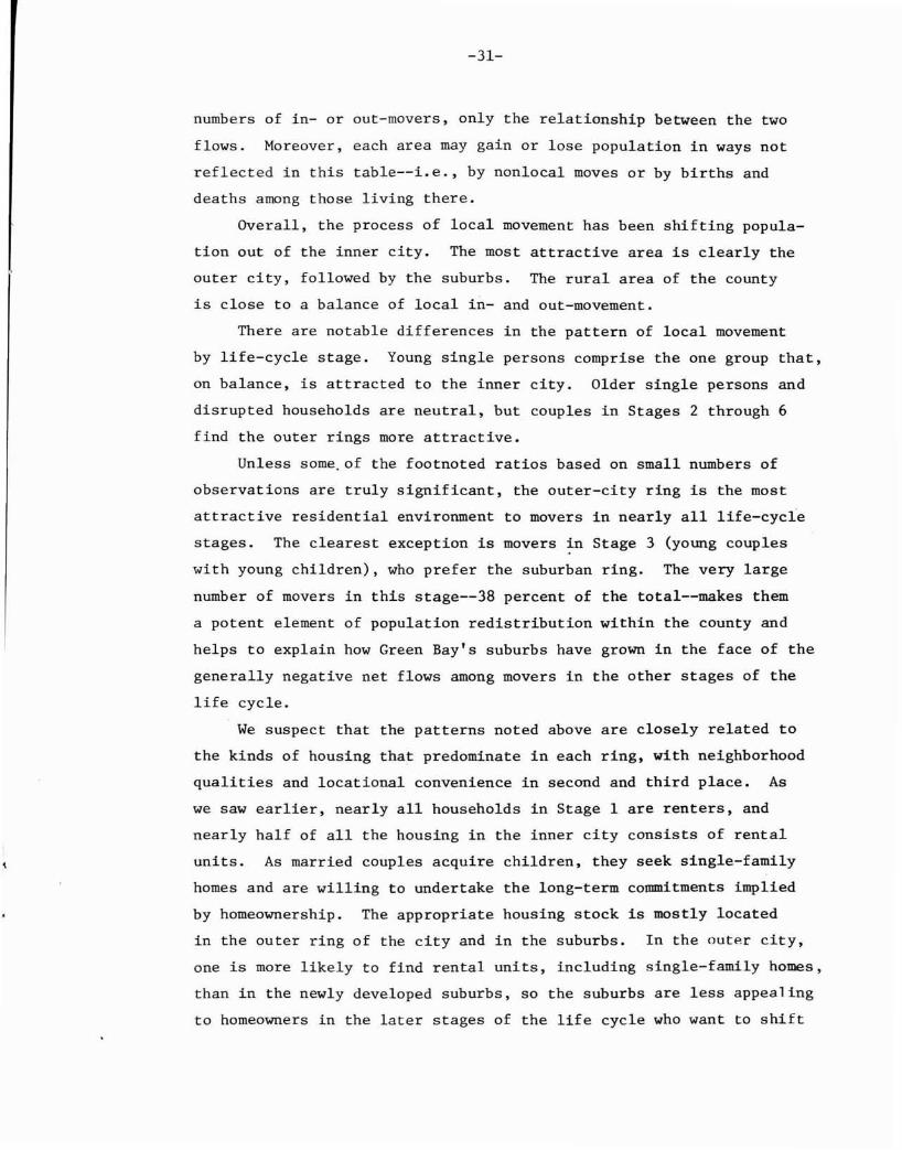
-31-

numbers of in- or out-movers, only the relationship between the two

flows. Moreover, each area may gain or lose population in ways not

reflected in this table--i.e., by nonlocal moves or by births and

deaths among those living there.

Overall, the process of local movement has been shifting popula­

tion out of the inner city. The most attractive area is clearly the

outer city, followed by the suburbs. The rural area of the county

is close to a balance of local in- and out-movement.

There are notable differences in the pattern of local movement

by life-cycle stage. Young single persons comprise the one group that,

on balance, is attracted to the inner city. Older single persons and

disrupted households are neutral, but couples in Stages 2 through 6

find the outer rings more attractive.

Unless some. of the footnoted ratios based on small numbers of

observations are truly significant, the outer-city ring is the most

attractive residential environment to movers in nearly all life-cycle

stages. The clearest exception is movers in Stage 3 (young couples

with young children), who prefer the suburban ring. The very large

number of movers in this stage--38 percent of the total--makes them

a potent element of population redistribution within the county and

helps to explain how Green Bay's suburbs have grown in the face of the

generally negative net flows among movers in the other stages of the

life cycle.

We suspect that the patterns noted above are closely related to

the kinds of housing that predominate in each ring, with neighborhood

qualities and locational convenience in second and third place. As

we saw earlier, nearly all households in Stage I are renters, and

nearly half of all the housing in the inner city consists of rental

units. As married couples acquire children, they seek single-family

homes and are willing to undertake the long-term commitments implied

by homeownership. The appropriate housing stock is mostly located

in the outer ring of the city and in the suburbs. In the outer city,

one is more likely to find rental units, including single-family homes,

than in the newly developed suburbs, so the suburbs are less appealing

to homeowners in the later stages of the life cycle who want to shift

-32-

back to rental tenure or to apartment living and who also want to be

close to retail stores, churches, and doctors' offices.

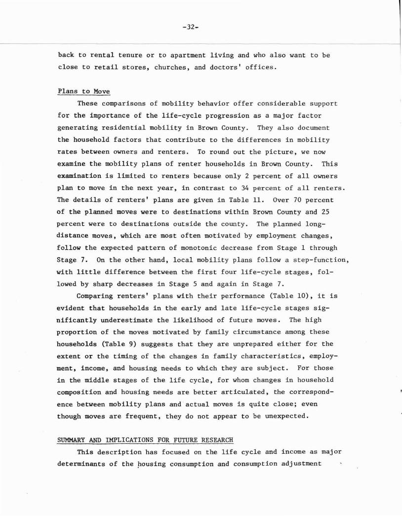
Plans to Move

These comparisons of mobility behavior offer considerable support

for the importance of the life-cycle progression as a major factor

generating residential mobility in Brown County. They also document

the household factors that contribute to the differences in mobility

rates between owners and renters. To round out the picture, we now

examine the mobility plans of renter households in Brown County. This

examination is limited to renters because only 2 percent of all owners

plan to move in the next year, in contrast to 34 percent of all renters.

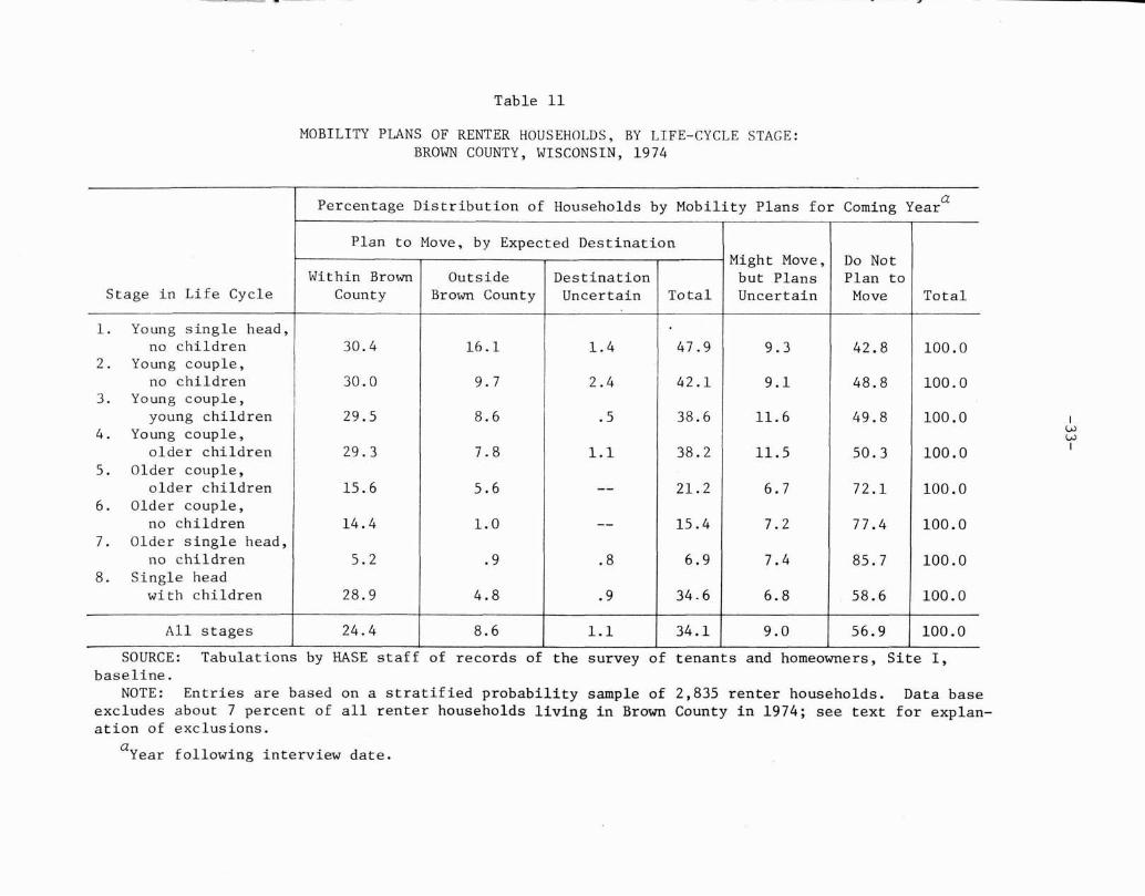
The details of renters' plans are given in Table 11. Over 70 percent

of the planned moves were to destinations within Brown County and 25

percent were to destinations outside the county. The planned long­

distance moves, which are most often motivated by employment changes,

follow the expected pattern of monotonic decrease from Stage 1 through

Stage 7. On the other hand, local mobility plans follow a step-function,

with little difference between the first four life-cycle stages, fol­

lowed by sharp decreases in Stage 5 and again in Stage 7.

Comparing renters' plans with their performance (Table 10), it is

evident that households in the early and late life-cycle stages sig­

nificantly underestimate the likelihood of future moves. The high

proportion of the moves motivated by family circumstance among these

households (Table 9) suggests that they are unprepared either for the

extent or the timing of the changes in family characteristics, employ­

ment, income, and housing needs to which they are subject. For those

in the middle stages of the life cycle, for whom changes in household

composition and housing needs are better articulated, the correspond­

ence between mobility plans and actual moves is quite close; even

though moves are frequent, they do not appear to be unexpected.

SUMMARY AND IMPLICATIONS FOR FUTURE RESEARCH

This description has focused on the life cycle and income as major

determinants of the ~ousing consumption and consumption adjustment

~_._-~'-- 7

Table 11

MOBILITY PLANS OF RENTER HOUSEHOLDS, BY LIFE-CYCLE STAGE:BROWN COUNTY, WISCONSIN, 1974

Percentage Distribution of Households by Mobility Plans for Coming Yeara

Plan to Move, by Expected DestinationMight Move, Do Not

Within Brown Outside Destination but Plans Plan toStage in Life Cycle County Brown County Uncertain Total Uncertain Move Total

1. Young single head,no children 30.4 16.1 1.4 47.9 9.3 42.8 100.0

2. Young couple,no children 30.0 9.7 2.4 42.1 9.1 48.8 100.0

3. Young couple,young children 29.5 8.6 .5 38.6 11. 6 49.8 100.0

4. Young couple,older children 29.3 7.8 1.1 38.2 11.5 50.3 100.0

5. Older couple,older children 15.6 5.6 -- 21. 2 6.7 72.1 100.0

6. Older couple,no children 14.4 1.0 -- 15.4 7.2 77 .4 100.0

7. Older single head,no children 5.2 .9 .8 6.9 7.4 85.7 100.0

8. Single headwi th children 28.9 4.8 .9 34.6 6.8 58.6 100.0

All stages 24.4 8.6 1.1 34.1 9.0 56.9 100.0

ILULUI

Tabulations by BASE staff of records of the survey of tenants and homeowners, Site I,

Entries are based on a stratified probability sample of 2,835 renter households. Data baseabout 7 percent of all renter households living in Brown County in 1974; see text for explan­exclusions.

SOURCE:baseline.

NOTE:excludesation of

a Year following interview date.

-34-

patterns in Brown County. Our data reveal a regular sequence in the

tenure, type, and size of units occupied over the life cycle. Young

single individuals typically set up their households in small rental

units in large multiunit buildings. As households progress to the

middle of the life cycle they adjust their consumption accordingly,

moving first to larger rental units (often single-family homes), then

buying a home. After peak household size is reached in the middle of

the life cycle, households begin to reduce their housing consumption

by moving to smaller single-family homes and rental units. Household

income affects the timing of this sequence of choices and the level of

expenditures more than the size or type of unit occupied.

Although our information on current consumption is based on longi­

tudinal inferences from cross-sectional data, retrospective data on the

mobility behavior of individual households support these basic findings

as to the frequency, type, and reasons for moving at different stages

of the life cycle.

These results provide a useful description of household consump­

tion choices at baseline. However, they are only the first step in

analyzing the effects of the allowance program on consumption patterns.

Several issues require further development.

First, differences in housing preferences within life-cycle stages

are important and must be examined in considerably more detail. Second,

tenure and type and size of unit by no means capture the range of varia­

tion in the housing stock of Brown County. Further work is needed to

identify specific housing attributes and their relative importance in

consumer decisions. Third, local mobility and its role in consumption

adjustment has only been skimmed in this paper. A more detailed exam­

ination of where households move, the differences in their housing at

origin and destination, and the role of search procedures is required.

Finally, the effect of housing allowances on all of these issues re­

mains to be analyzed.

..

-35-

Appendix

HOUSING TENURE, LIFE-CYCLE STAGE, AND INCOME

Tabulations presented in the main text of this paper indicate that

housing tenure varies systematically over life-cycle stages: Ninety­

four percent of all households in Stage 1 are renters, but by Stage 5,

over 95 percent are owners; in later stages, the proportion of owners

decreases nearly to 60 percent.

However, our tabulations also show that several variables that

might affect a household's current tenure follow a similar pattern, at

first increasing, then decreasing over life-cycle stages. These include

household size, number of employed persons, and household income. It

is possible that the life-cycle variable acts as a proxy for one or more

of these other variables and has little or no independent power to dis­

tinguish owners from renters.

To test this hypothesis, we estimated the coefficients of a

linear regression model in which the dependent variable is housing

tenure, having a value of 1 for homeowners and zero for renters. The

independent variables in the model are the household's stage in the

life cycle and selected other household characteristics. We used a

two-stage generalized least squares (GLS) method to estimate the co­

efficients of the model; this method is more efficient than ordinary

least squares (OLS) for estimating a linear probability function. 9

9We used a two-step GLS procedure. In the first step, we usedOLS to estimate the probability that a household was a homeowner(yJ, given the values of the independent variables for each observation.In the second step, we weighted both the dependent and independentvariables of each observation by [y(1-YJ]-·5, then reestimated thecoefficients using OLS.

Goldberger [7] shows that this procedure corrects for theheteroscedasticity of the error terms that occurs when the dependentvariable is binary. One difficulty with this procedure is that thereis no guarantee that the estimated probabilities in the first stepwill fall in the closed interval [0,1]. We assigned the values .01and .99 to those estimated probabilities that fell outside this inter­val. Smith [18] used Monte Carlo methods to evaluate the effectsof this assignment rule on the estimators and finds them to be smalland to diminish as sample si,:e increases.

Note that the use of a nonlinear estimating procedure such aslogit analysis can yield still more efficient estimators than 'hosewe present. However, the computational expense of a nonlinear methodwas not justifiable for this preliminary analysis.

-36-

The independent variables used to predict tenure in this model

are also binary, with two exceptions. -The binary variables include

dummy variables identifying the household's life-cycle stage, with

Stage 2 as the standard case which is therefore not explicitly in­

cluded; the employment status of the household head; the employment

status of the spouse in households headed by couples; and whether or

not the household plans to move during the coming year. As a supple­

ment to the life-cycle classification of households by the presence or

absence of children in the household, we have included the number of

children as a variable. Finally, household income in 1973 (the year

preceding the survey) is included. Two variables describing the

education status of the household head--number of years of schooling

and current enrollment status--are omitted here because preliminary

results indicated that they were of little help in predicting tenure.

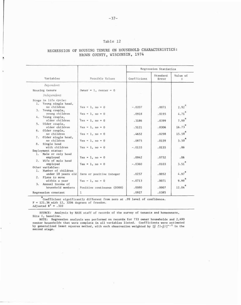
The results of this regression are reported in Table 12. They

clearly indicate that the life-cycle variables reflect important

differences in tenure preferences that are independent of other house­

hold characteristics, including income. Except for Stage 8 (disrupted

households), the coefficients of the life-cycle variables are all sig­

nificantly different from zero and generally different from each other;lO

and their values are consistent with our earlier account of the changing

pattern of tenure over the life cycle.

The head's employment status has no effect on the probability that

the household is currently an owner. This is not surprising, because

the effect of income is held constant. On the other hand, the coeffic­

ient on the wife's employment status is significant and negative.

lOAlthough Table 12 shows the results of tests for coefficientsthat are significantly different from zero, it does not show theresults of pairwise tests for significant differences between the valuesof the coefficients for different life-cycle stages. Standard testsindicated significant differences between all pairs except Stages 3and 7, 5 and 6, and 1 and 8. Recall that the coefficient for Stage 8is also not significantly different from zero.

-37-

Table 12

REGRESSION OF HOUSING TENURE ON HOUSEHOLD CHARACTERISTICS:BROWN COUNTY, WISCONSIN, 1974

Regression Statistics

Standard Value ofVariables Possible Values Coefficient Error t

Dependent

Housing tenure Owner = 1, renter = 0

Independent

Stage in life cycle:1- Young single head,

*no children Yes = 1, no = 0 -.0207 .0071 2.923. Young couple,

*young children Yes = I, no = 0 .0918 .0195 4.714. Young couple,

*older children Yes = 1, no = 0 .3186 .0399 7.995. Older couple,

*older children Yes = 1, no = 0 .5121 .0306 16.736. Older couple,

*no children Yes = 1, no = 0 .4652 .0298 15.587. Older single head,

*no children Yes = 1, no = 0 .0875 .0159 5.508. Single head

with children Yes = 1, no = 0 -.0133 .0155 .86Employment status:

1- Male or only heademployed Yes = 1, no = 0 .0042 .0752 .06

2. Wife of male head*employed Yes = 1, no = 0 -.0360 .0103 3.51

Other variables:1- Number of children

*under 18 years old Zero or positi.ve integer .0257 .0052 4.972. Plans to move

*within a year Yes = 1, no = 0 -.0713 .0071 9.993. Annual income of

*household members Positive continuous ($000) .0080 .0007 12.04

Regression constant 1 .0927 .0385

*Coefficient significantly different from zero at .99 level of confidence.F = 121.36 wLth 12, 3206 degrees of freedon.Adjusted RZ = .310

SOURCE: Analysis by HASE staff of records of the survey of tenants and homeowners,Site I, baseline.

NOTE: Regression analysis was performed on records for 733 owner households and 2,490renter households that were complete in all variables listed. Coefficients were estimatedby generalized least squares method, with each observation weighted by [y (l_YJj-·s in thesecond stage.

-38-

This coefficient may reflect a history of uncertain earnings by the

husband that leads the wife to work in order to supplement household

income. Such a couple would probably be hesitant to obligate a fixed

amount over time to mortgage payments and hence is more likely to

rent. On the other hand, working couples may simply prefer the less

onerous domestic duties of renters.

The coefficient on the number of minors in the household is posi­

tive and significant. An increase in the number of minors may increase

the likelihood that the household is a homeowner for either of two

reasons. First, a larger family requires more space, and would be

more likely to seek a single-family home; and there are indications

from other studies that single-family homes are cheaper to own than

to rent, at least in terms of out-of-pocket costs. Second, this

variable may act as a proxy for the age of the head. Older heads are

likely to be more settled and as a consequence to be homeowners; they

are also likely to have larger families.

The negative coefficient on the variable that represents the

household's near-term mobility plans is difficult to interpret. The

variable appears to be endogenous to the equation and therefore simul­

taneous equations bias may affect the value of the coefficient. Renters

are more likely to move than homeowners because they have lower moving

costs--they do not have to sell their current residences and pay the

transaction costs. In its present form, the coefficient indicates only

that renters are more likely to move, not that current mobility plans

are a significant indicator of current tenure status.

The relationship between current household income and housing

tenure is statistically significant but amazingly small. A family

with an income of $16,000 is more likely to own its home than a family

with an income of $8,000, but the incremental probability is only

.064. We would been less surprised to find a larger coefficient with

a larger standard error; while homeownership cannot readily be inter­

preted as affecting income, neither is it clear that current income

had much relevance to the earlier decision to buy; at best, it indi­

cates the household's ability to keep up mortgage payments.

-39­

Because nearly all homeowners live in single-family houses, it

is reasonable to wonder whether the regression model reported above

is misspecified in its dependent variable. That is, we may be

observing the factors that influence the probability that a household

will occupy a single-family home, rather than its probability of

homeownership.

One way to test for such a misspecification is to focus on the

sample of renter households, most of whom live in multiple dwellings

but about 15 percent of whom live in single-family houses. Using

records for renters only, we replaced tenure in the regression model

with a binary variable for occupancy of a single-family house, then

estimated the coefficients of the altered model. If the coefficients

did not change much from those in Table 12, we would conclude that

the misspecificat~on was likely.

There was no resemblance between the two sets of coefficients.

In the altered model, the only variables with significant coefficients

were: life-cycle Stages 1, 4, 5, and 6; number of minors; and plans

to move. Differences in household income had no apparent effect on

the likelihood that a renter household would occupy a single-family

house. We do not think that tenure is acting as a proxy for type

of housing in the original model.

-41-

REFERENCES

~

I

[1] Burgess, E. W. "The Growth of the City."Burgess, and R. D. McKenzie, The City.of Chicago Press, 1925.

In R. E. Park, E. W.Chicago: University

[2 ] Butler, E. W. et al.A National Survey.1969.

Moving Behavior and Residential Choice:Highway Research Board, Report No. 81,

[3] Carliner, G. "Determinants of Home Ownership," Land Economics,Vol. 50 (1974), pp. 109-119.

[4] Chevan, A. "Family Growth, Household Density and Moving,"Demography, Vol. 8 (1971), pp. 451-458.

[5] David, M. H. Family Composition and Consumption. Amsterdam:North Holland Publishing Company, 1962.

[6] Gans, H. J. The Levittowners. New York: Random House, 1967.

[7] Goldberger, A. Econometric Theory. New York: J. Wiley andSons, 1964.

[8] Greenbie, B. B. "New Homes or New Neighborhoods? A Survey ofPriorities Among Home Owners in Madison, Wisconsin," LandEconomics, Vol. 45 (1969), pp. 359-365.

[9] Guest, A. M. "Patterns of Family Location," Demography, Vol. 9(1972), pp. 159-171.

[10] Kain, J. and J. Quigley. "Housing Market Discrimination, HomeOwnership and Savings Behavior," American Economic Review,Vol. 60 (1972), pp. 263-277.

[11] Lansing, J. B. and J. N. Morgan. "Consumer Finances Over theLife Cycle." In L. Clark (Ed.), The Life Cycle and ConsumerBehavior. New York: New York University Press, 1955.

[12] Lansing, J. B. and L. Kish. "Family Life Cycle as an IndependentVariable," American Sociological Review, Vol. 22 (1957), pp.512-519.

[13] Morgan, J. N. (Ed.). Five Thousand American Families: Patternsof Economic Progress~ Vol. II. Ann Arbor: Survey ResearchCenter, Institute for Survey Research, 1972.

[14] Pickvance, C. G. "Life Cycle, Housing Tenure, and ResidentialMobility: A Path Analytic Approach," Urban Studies, Vol. 11(1974), pp. 171-188.

-42-

[15] Rossi, P. Why Families Move. Glencoe: The Free Press, 1955.

[16] Schnore, L. F. The Urban Scene. New York: The Free Press,1965.

[17] Shelton, J. B. "The Costs of Renting Versus Owning a Horne,"Land Economics~ Vol. 44 (1968), pp. 59-72.

[18] Smith, V. K. Monte Carlo Methods. Lexington: Lexington Books,1974.

[19] Speare, A., Jr., "Horne Ownership, Life Cycle Stage and ResidentialMobility," Demography~ Vol. 7 (1970), pp. 449-457.

[20] Struyk, R. J. and S. Marshall. "The Determinants of HouseholdHome Ownership," Urban Studies, Vol. 11 (1974), pp. 289-299.

[21] U.S. Bureau of the Census. "Reasons for Moving: March 1962 toMarch 1963," Current Population Reports, Series P-20, No. 154,1966.

[22] "Population of the United States Trends and Prospects:1950-1970," Current Population Reports~ Series P-23, No. 49,1974.

[23] "Households and Families by Type: March 1974," CurrentPopulation Reports, Series P-20, No. 266, 1975.