Policy Research Working Paper 8430

Household Expenditure and Poverty Measures in 60 Minutes

A New Approach with Results from Mogadishu

Utz PapeJohan Mistiaen

Poverty and Equity Global PracticeMay 2018

WPS8430P

ublic

Dis

clos

ure

Aut

horiz

edP

ublic

Dis

clos

ure

Aut

horiz

edP

ublic

Dis

clos

ure

Aut

horiz

edP

ublic

Dis

clos

ure

Aut

horiz

ed

Produced by the Research Support Team

Abstract

The Policy Research Working Paper Series disseminates the findings of work in progress to encourage the exchange of ideas about development issues. An objective of the series is to get the findings out quickly, even if the presentations are less than fully polished. The papers carry the names of the authors and should be cited accordingly. The findings, interpretations, and conclusions expressed in this paper are entirely those of the authors. They do not necessarily represent the views of the International Bank for Reconstruction and Development/World Bank and its affiliated organizations, or those of the Executive Directors of the World Bank or the governments they represent.

Policy Research Working Paper 8430

This paper is a product of the Poverty and Equity Global Practice. It is part of a larger effort by the World Bank to provide open access to its research and make a contribution to development policy discussions around the world. Policy Research Working Papers are also posted on the Web at http://www.worldbank.org/research. The authors may be contacted at upape@worldbank.org.

In fragile states and areas beset by insecurity and conflict, the time available for a face-to-face interview is typically limited. That prevents administering the lengthy household consumption expenditure surveys used for measuring pov-erty. This paper presents a new approach to obtain unbiased estimates of poverty when the time to conduct interviews is a binding constraint. The finite list of consumption recall items is partitioned selectively into a core module and algo-rithmically into nonoverlapping optional modules. Each

household is systematically assigned the core module and randomly assigned one of the optional modules. Multi-ple imputation techniques are then used to estimate total household consumption. Based on ex post simulations, the approach is demonstrated to yield reliable estimates of per capita consumption and poverty using data from a regular household budget survey collected in Hargeisa, Somaliland. The approach is then applied to a survey conducted in Mog-adishu where interview time could not exceed 60 minutes.

HouseholdExpenditureandPovertyMeasuresin60Minutes:ANewApproachwithResultsfromMogadishu

Utz Pape and Johan Mistiaen1 

Keywords: Poverty and inequality measurement, survey methods   

JEL: C83, D63, I32. 

1 Corresponding author: Utz Pape (upape@worldbank.org). The findings, interpretations and conclusions expressed in this paper are entirely those of the authors, and do not necessarily represent the views of the World Bank, its Executive Directors, or the governments of the countries they represent. 

2  

Introduction

Poverty is the paramount indicator to gauge the socioeconomic well‐being of a population. Especially after 

a shock, poverty estimates can disentangle who in the population was affected how severely. As one of 

the main indicators for poverty, monetary poverty is measured by a welfare aggregate usually based on 

consumption in developing countries and a poverty line. The poverty line indicates the minimum level of 

welfare required for a healthy living. 

Consumption aggregates are estimated traditionally by time‐consuming household consumption surveys. 

A household consumption questionnaire records consumption and expenditures for a comprehensive list 

of food and non‐food items. With around 300 to 400 items, the administering time of the questionnaire 

often exceeds 90 – 120 minutes. In addition to higher costs due to longer administering time, response 

fatigue can increase measurement error especially for items at the end of the questionnaire. In a fragile 

country context, a face‐to‐face time of 90 – 120 minutes can be prohibitively high. For example, security 

concerns restricted the duration of a visit in Mogadishu to about 60 minutes.  

The  extensive  nature of  household  consumption  surveys makes  it  difficult  to  obtain  updated poverty 

estimates especially when they are needed the most: after a shock and in fragile countries. Therefore, 

approaches were developed to reduce administering time to allow collection of consumption data with 

significantly lower administering time. The most straightforward approach to minimize administering time 

reduces  the number of  items either by asking  for aggregates or by skipping  less  frequently consumed 

items,  called  reduced  consumption  methodology.  However,  both  approaches  have  been  shown  to 

underestimate  consumption, which  in  turn  overestimates  poverty.2  Splitting  up  the  questionnaire  for 

multiple visits  is another solution but attrition issues – especially  in fragile country contexts – increase 

required  sample  size  and  also  have  a  high  cost  implication.  In  addition,  multiple  visits  to  the  same 

household can increase security concerns. 

A second class of approaches utilizes a full consumption baseline survey and updates poverty estimates 

based  on  a  small  subset  of  collected  indicators.3  These  approaches  estimate  a welfare model  on  the 

baseline survey using a small number of easy‐to‐collect indicators. This allows updating poverty estimates 

by collecting only the set of indicators instead of direct consumption data. While the approach is cost‐

efficient and easy to implement in normal circumstances, the approach has two major drawbacks in the 

                                                            2 Beegle et al, 2012. 3 Douidich et al, 2013; SWIFT. 

3  

context of fragility and shocks. First, the approach requires a baseline survey, which is sometimes – for 

example in Mogadishu – not existent. Second, the approach relies on a structural model estimated from 

the baseline survey.4 In the case of shocks, the structural assumptions, which cannot be tested, are often 

violated. Thus, poverty updates based on the violated assumption tend to under‐estimate the impact of 

the shock on poverty. Therefore, cross‐survey imputation methodologies are not applicable in the context 

of shocks and fragility.  

A new methodology is proposed combining an innovative questionnaire design with standard imputation 

techniques.  This  substantially  reduces  the  administering  time  of  a  consumption  survey  to  about  60 

minutes while at the same time credible poverty estimates are obtained. Thus, the gain in administering 

time is bought by the need to impute missing consumption values. Due to the design of the questionnaire, 

the method circumvents systematic biases as identified for alternative methodologies.  

After explaining the methodology in more detail in the next section, the performance of the methodology 

is assessed ex post using collected household budget data in Hargeisa, Somalia. Next, the methodology is 

applied  to  newly  collected  data  in  Mogadishu,  Somalia,  where  full  consumption  data  collection  was 

impossible due  to  security  constraints.  The  consistency of  the  consumption estimates  is  evaluated by 

performing  validity  checks.  A  conclusion  discusses  the  limitations  of  the  methodology,  the  benefits 

especially in combination of using CAPI technology and the need for further research.  

Methodology

Overview

The rapid consumption survey methodology consists of five main steps (Figure 1). First, core items are 

selected based on their importance for consumption. Second, the remaining items are partitioned into 

optional modules. Third, optional modules are assigned to groups of households. After data collection, 

fourth, optional consumption modules are imputed for all households. Fifth, the resulting consumption 

aggregate is used to estimate poverty indicators. 

                                                            4 Christiaensen et al, 2010; Christiaensen et al, 2011. 

4  

First, core consumption items are selected. Consumption in a country bears some variability but usually a 

small number of a few dozen items captures the majority of consumption. These items are assigned to 

the core module, which will be administered to all households. Important items can be identified by the 

average  food  share  per  household  or  across  households.  Previous  consumption  surveys  in  the  same 

country or consumption shares of neighboring / similar countries can be used to estimate food shares.5  

                                                            5 As shown later, the assignment of items to modules is very robust and, thus, even rough estimates of consumption shares are sufficient to inform the assignment without requiring a baseline survey. 

Consumption 

Module Core Module Opt Module 1 Opt Module 2

Item 1 Item C1 Item D1 Item E1

Item 2 Item C2 Item D2 Item E2

… … … …

Item N Item CX Item DY Item EZ

Household 

Group 1

Household 

Group 2

Core Module Core Module

Opt Module 1

Opt Module 2

Household 

Group 1

Household 

Group 2

Core Module Imputation Core Module

Opt Module 1 Opt Module 1

Opt Module 2 Opt Module 2

Household 

Group 1'

Household 

Group 2'

Core Module Imputation Core Module

Opt Module 1 Opt Module 1

Opt Module 2 Opt Module 2

… …

Household 

Group 1''

Household 

Group 2''

Core Module Imputation Core Module

Opt Module 1 Opt Module 1

Opt Module 2 Opt Module 2

Questionnaire

Survey

Imputation

Multiple Im

putation

Income

Estimated

Real

Income

Imputation 1

Imputation 2

Imputation 3

Imputation 4

Real

Figure 1: Illustration of the rapid consumption survey methodology (using illustrative data only). The consumption module ispartitioned into core and optional modules, which in turn are assigned to households. Consumption is imputed utilizing thesub‐sample information of the optional modules either by single or multiple imputation methods. 

5  

Second, non‐core  items are partitioned  into optional modules. Different methods can be used  for  the 

partitioning into optional modules.  In the simplest case, the remaining items are ordered according to 

their  food  share  and  assigned  one‐by‐one  while  iterating  the  optional module  in  each  step.  A more 

sophisticated  method  would  take  into  account  correlation  between  items  and  partition  them  into 

orthogonal sets per module. This would lead to high correlation between modules supporting the total 

consumption estimation.  

Conceptual division into core and optional items should not be reflected in the layout of the questionnaire. 

More complicated partition patterns can result in a set of very different items in each module. However, 

the  modular  structure  should  not  influence  the  layout  of  the  questionnaire.  Instead,  all  items  per 

household will be grouped into categories of consumption items (like cereals) and different recall periods. 

Therefore, it is recommended to use CAPI technology, which allows hiding the modular structure of the 

consumption module from the enumerator.  

Third, optional modules will be assigned to groups of households. Assignment of optional modules will be 

performed randomly stratified by enumeration areas to ensure appropriate representation of optional 

modules in each enumeration area. This step is followed by the actual data collection. 

Fourth,  household  consumption  will  be  estimated  by  imputation.  The  average  consumption  of  each 

optional module  can  be  estimated  based  on  the  sub‐sample  of  households  assigned  to  the  optional 

module.  In  the  simplest  case,  a  simple  average  can be estimated. More  sophisticated  techniques  can 

employ  a welfare model  based  on  household  characteristics  and  consumption  of  the  core  items.  Six 

techniques are presented in the next section and perform their estimation on the data set from Hargeisa. 

Single imputation of the consumption aggregate under‐estimates the variance of household consumption. 

Depending on the location of the poverty  line relative to the consumption distribution, this can either 

consistently under‐ or over‐estimate poverty. Multiple imputation based on boot‐strapping can mitigate 

the problem but will render analysis more complicated. Single as well as multiple imputation techniques 

are used for the evaluation of the methodology. 

ModuleConstruction

Consumption for a household is estimated by the sum of expenditures for a set of items 

 

6  

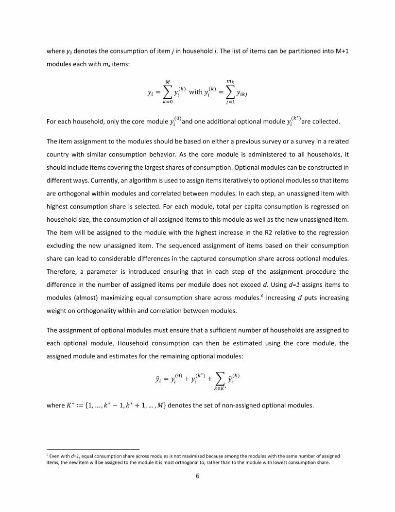
where yij denotes the consumption of item j in household i. The list of items can be partitioned into M+1 

modules each with mk items: 

with  

For each household, only the core module  and one additional optional module ∗are collected.  

The item assignment to the modules should be based on either a previous survey or a survey in a related 

country with  similar  consumption  behavior.  As  the  core module  is  administered  to  all  households,  it 

should include items covering the largest shares of consumption. Optional modules can be constructed in 

different ways. Currently, an algorithm is used to assign items iteratively to optional modules so that items 

are orthogonal within modules and correlated between modules. In each step, an unassigned item with 

highest consumption share  is selected. For each module, total per capita consumption is regressed on 

household size, the consumption of all assigned items to this module as well as the new unassigned item. 

The  item will be assigned to the module with the highest  increase  in the R2 relative to the regression 

excluding  the new unassigned  item. The  sequenced assignment of  items based on  their  consumption 

share can lead to considerable differences in the captured consumption share across optional modules. 

Therefore,  a  parameter  is  introduced  ensuring  that  in  each  step  of  the  assignment  procedure  the 

difference in the number of assigned items per module does not exceed d. Using d=1 assigns items to 

modules  (almost) maximizing  equal  consumption  share  across modules.6  Increasing d  puts  increasing 

weight on orthogonality within and correlation between modules. 

The assignment of optional modules must ensure that a sufficient number of households are assigned to 

each  optional  module.  Household  consumption  can  then  be  estimated  using  the  core  module,  the 

assigned module and estimates for the remaining optional modules: 

∗

∈ ∗

 

where  ∗ ∶ 1, … , ∗ 1, ∗ 1, … ,  denotes the set of non‐assigned optional modules.  

                                                            6 Even with d=1, equal consumption share across modules is not maximized because among the modules with the same number of assigned items, the new item will be assigned to the module it is most orthogonal to; rather than to the module with lowest consumption share. 

7  

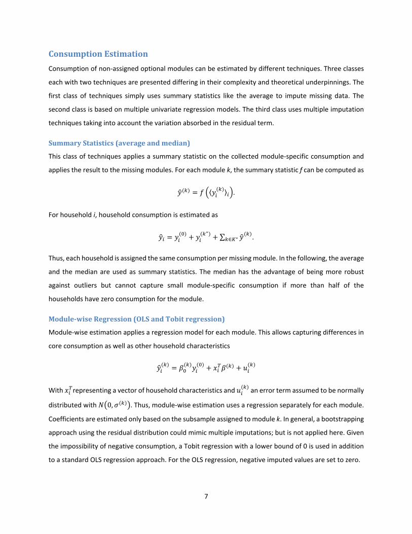
ConsumptionEstimation

Consumption of non‐assigned optional modules can be estimated by different techniques. Three classes 

each with two techniques are presented differing in their complexity and theoretical underpinnings. The 

first  class  of  techniques  simply  uses  summary  statistics  like  the  average  to  impute missing  data.  The 

second class is based on multiple univariate regression models. The third class uses multiple imputation 

techniques taking into account the variation absorbed in the residual term.  

SummaryStatistics(averageandmedian)

This class of techniques applies a summary statistic on the collected module‐specific consumption and 

applies the result to the missing modules. For each module k, the summary statistic f can be computed as 

⟨ ⟩ . 

For household i, household consumption is estimated as 

∗∑ ∈ ∗ . 

Thus, each household is assigned the same consumption per missing module. In the following, the average 

and  the median are used as  summary  statistics. The median has  the advantage of being more  robust 

against  outliers  but  cannot  capture  small  module‐specific  consumption  if  more  than  half  of  the 

households have zero consumption for the module. 

Module‐wiseRegression(OLSandTobitregression)

Module‐wise estimation applies a regression model for each module. This allows capturing differences in 

core consumption as well as other household characteristics 

 

With  representing a vector of household characteristics and   an error term assumed to be normally 

distributed with  0, . Thus, module‐wise estimation uses a regression separately for each module. 

Coefficients are estimated only based on the subsample assigned to module k. In general, a bootstrapping 

approach using the residual distribution could mimic multiple imputations; but is not applied here. Given 

the impossibility of negative consumption, a Tobit regression with a lower bound of 0 is used in addition 

to a standard OLS regression approach. For the OLS regression, negative imputed values are set to zero. 

8  

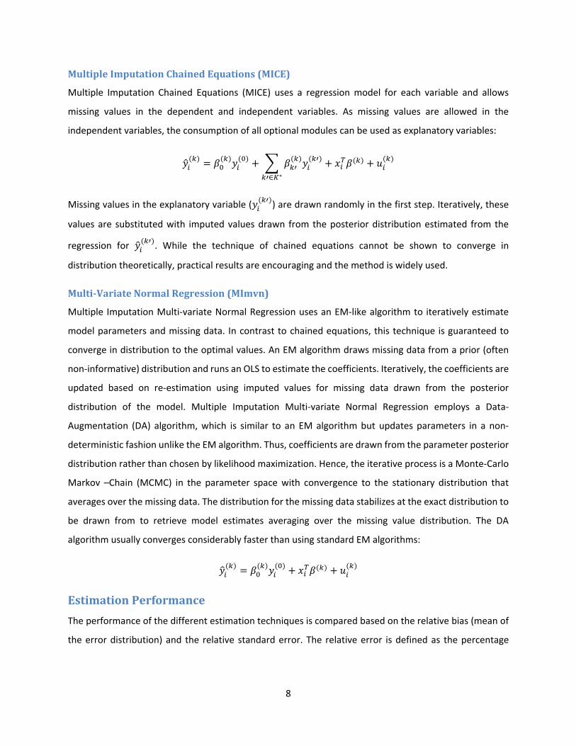
MultipleImputationChainedEquations(MICE)

Multiple  Imputation  Chained  Equations  (MICE)  uses  a  regression model  for  each  variable  and  allows 

missing  values  in  the  dependent  and  independent  variables.  As  missing  values  are  allowed  in  the 

independent variables, the consumption of all optional modules can be used as explanatory variables:  

∈ ∗

 

Missing values in the explanatory variable ( ) are drawn randomly in the first step. Iteratively, these 

values are  substituted with  imputed values drawn  from the posterior distribution estimated  from the 

regression  for  .  While  the  technique  of  chained  equations  cannot  be  shown  to  converge  in 

distribution theoretically, practical results are encouraging and the method is widely used. 

Multi‐VariateNormalRegression(MImvn)

Multiple  Imputation Multi‐variate Normal Regression uses an EM‐like algorithm to  iteratively estimate 

model parameters and missing data.  In contrast to chained equations, this technique is guaranteed to 

converge in distribution to the optimal values. An EM algorithm draws missing data from a prior (often 

non‐informative) distribution and runs an OLS to estimate the coefficients. Iteratively, the coefficients are 

updated  based  on  re‐estimation  using  imputed  values  for  missing  data  drawn  from  the  posterior 

distribution  of  the  model.  Multiple  Imputation  Multi‐variate  Normal  Regression  employs  a  Data‐

Augmentation  (DA)  algorithm, which  is  similar  to  an  EM algorithm but  updates  parameters  in  a  non‐

deterministic fashion unlike the EM algorithm. Thus, coefficients are drawn from the parameter posterior 

distribution rather than chosen by likelihood maximization. Hence, the iterative process is a Monte‐Carlo 

Markov  –Chain  (MCMC)  in  the  parameter  space with  convergence  to  the  stationary  distribution  that 

averages over the missing data. The distribution for the missing data stabilizes at the exact distribution to 

be  drawn  from  to  retrieve  model  estimates  averaging  over  the  missing  value  distribution.  The  DA 

algorithm usually converges considerably faster than using standard EM algorithms: 

 

EstimationPerformance

The performance of the different estimation techniques is compared based on the relative bias (mean of 

the error distribution) and  the  relative  standard error. The  relative error  is defined as  the percentage 

9  

difference of the estimated consumption and the reference consumption (based on the full consumption 

module): 

 

The relative bias is the average of the relative error: 

1

 

The relative standard error is the standard deviation of the relative error: 

1 

For estimation based on multiple imputations,   is averaged over all imputations.  

Each proposed estimation procedure is run on random assignments of households to optional modules. 

A constraint ensures that each optional module is assigned equally often to a household per enumeration. 

The relative bias and the relative standard error are reported across all simulations. 

The performance measures can be calculated at different levels. At the household level, the relative error 

is the relative difference in the household consumption. At the cluster level, the relative error is defined 

as  the  relative  difference  of  the  average  reference  household  consumption  and  average  estimated 

household consumption across the households in the cluster. Similarly, the global level compares total 

average consumption for all households.  

Results

In  this  section,  the  rapid  consumption methodology will  first  be  applied  to  a data  set  including  a  full 

consumption module from Hargeisa, Somalia. This will be used to assess the performance of the rapid 

consumption methodology compared to the traditional full consumption. Subsequently, the results from 

the High Frequency Survey in Mogadishu are presented. Security risks restrict face‐to‐face interview time 

to less than one hour. Therefore, the rapid consumption methodology is employed to derive the first ever 

10  

consumption  estimates  for  Mogadishu.  The  resulting  consumption  aggregate  is  presented  with 

consistency checks for its validation. 

ExpostSimulation

The rapid consumption methodology is applied ex post to household budget data collected in Hargeisa, 

Somalia. Hargeisa was chosen as it is the most similar city to Mogadishu. Using the full consumption data 

set from Hargeisa allows a full‐fledged assessment of the new methodology. Based on selected indicators, 

the results are compared after estimating consumption based on the rapid consumption methodology 

with  the  results  from using  the  traditional  full  consumption module. A  comparison  is  added with  the 

results for a reduced consumption module. 

The simulation assigns each household to one optional module. The consumption data for the modules 

not assigned to the household is deleted. Multiple simulations are performed with varying assignment of 

modules  to  households.  Across  the  simulations,  three  consumption  aggregates  and  four  poverty  and 

inequality indicators are calculated. The consumption indicators capture the accuracy of the estimation 

at three different levels: the household level, the cluster level (consisting of about 9 households) and the 

level of the data set. In addition, the poverty headcount (FGT0), poverty depth (FGT1) and poverty severity 

(FGT2) as well as the Gini coefficient are calculated to capture inequality. 

The six proposed estimation  techniques presented  in  the previous section are compared based on 20 

simulations with respect to their relative bias and relative standard error. All simulations used the same 

item assignment to modules using the algorithm as described with parameter d=3 (see Table 1 for the 

resulting consumption shares per module).7 The estimation  techniques differ  considerably  in  terms of 

performance. The techniques are also compared to using a reduced consumption module where the same 

consumption items are collected for all households. The number of items is equal to the size of the core 

and one optional module implying a comparable face‐to‐face interview time to the Rapid Consumption 

methodology. 

                                                            7 Robustness checks are performed with different item assignment to modules including setting the parameter d=1 and d=2. The estimation results are extremely robust to changes in the item assignment to modules. 

11  

Table 1: Number of items and consumption share captured per module. 

  Food  Non Food 

  Number 

of Items 

Share of 

Consumption 

Number of 

Items 

Share of 

Consumption 

Core  33  92%  25  88% 

Module 1  17  3%  15  3% 

Module 2  17  2%  15  3% 

Module 3  15  2%  15  4% 

Module 4  17  2%  15  3% 

 

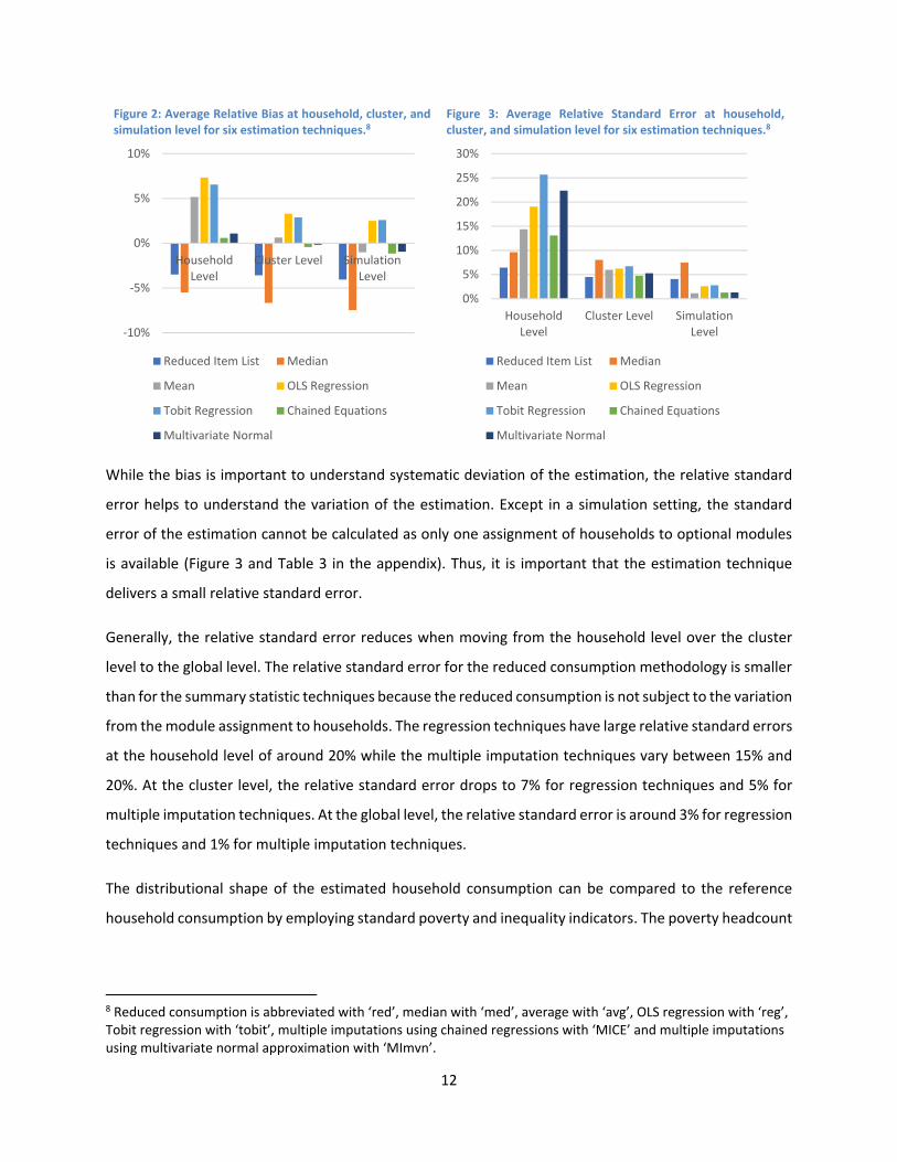
Comparing  the  reduced  consumption  approach  with  the  full  consumption  as  reference,  the  reduced 

consumption approach suffers from an under‐estimation of the consumption (Figure 2 and Table 3 in the 

appendix). This is not surprising because the approach only collects consumption from a subset of items. 

Applying  the  median  as  a  summary  statistic  also  results  in  an  under‐estimation  of  consumption.  As 

consumption distributions have a long right tail, the median consumption belongs to a poorer household 

than the average household.  In the case of Hargeisa, several optional modules have a median of zero 

consumption. Thus, the median underestimates the consumption similarly to the reduced consumption 

approach.  In  contrast,  the  average  consumption of  households  is  larger  than  the  consumption of  the 

median household. Thus, it  is not surprising that the technique using the average as summary statistic 

over‐estimates total consumption at the household and cluster level.  

The regression techniques have a similar performance with a considerable upward bias at all levels. The 

Tobit  regression performs slightly better at  the household and cluster  level.  In contrast, both multiple 

imputation techniques perform exceptionally well with a bias below 1% at all levels. 

12  

Figure 2: Average Relative Bias at household, cluster, and simulation level for six estimation techniques.8 

 

Figure  3:  Average  Relative  Standard  Error  at  household, cluster, and simulation level for six estimation techniques.8 

 

While the bias is important to understand systematic deviation of the estimation, the relative standard 

error helps to understand the variation of  the estimation. Except  in a simulation setting, the standard 

error of the estimation cannot be calculated as only one assignment of households to optional modules 

is available (Figure 3 and Table 3  in the appendix). Thus,  it  is  important that the estimation technique 

delivers a small relative standard error.  

Generally,  the relative standard error reduces when moving from the household  level over the cluster 

level to the global level. The relative standard error for the reduced consumption methodology is smaller 

than for the summary statistic techniques because the reduced consumption is not subject to the variation 

from the module assignment to households. The regression techniques have large relative standard errors 

at the household level of around 20% while the multiple imputation techniques vary between 15% and 

20%. At the cluster level, the relative standard error drops to 7% for regression techniques and 5% for 

multiple imputation techniques. At the global level, the relative standard error is around 3% for regression 

techniques and 1% for multiple imputation techniques.  

The distributional  shape of  the  estimated household  consumption  can be  compared  to  the  reference 

household consumption by employing standard poverty and inequality indicators. The poverty headcount 

                                                            8 Reduced consumption is abbreviated with ‘red’, median with ‘med’, average with ‘avg’, OLS regression with ‘reg’, Tobit regression with ‘tobit’, multiple imputations using chained regressions with ‘MICE’ and multiple imputations using multivariate normal approximation with ‘MImvn’. 

‐10%

‐5%

0%

5%

10%

HouseholdLevel

Cluster Level SimulationLevel

Reduced Item List Median

Mean OLS Regression

Tobit Regression Chained Equations

Multivariate Normal

0%

5%

10%

15%

20%

25%

30%

HouseholdLevel

Cluster Level SimulationLevel

Reduced Item List Median

Mean OLS Regression

Tobit Regression Chained Equations

Multivariate Normal

13  

(FGT0) is 57.4% for the reference distribution.9 Not surprisingly, the reduced consumption and the median 

summary  statistic  overestimate  poverty  by  several  percentage  points  due  to  the  under‐estimation  of 

consumption (Figure 4 and Table 4 in the appendix). The average summary statistic and the regression 

techniques  underestimate  poverty  since  they  overestimate  consumption.  The  multiple  imputation 

techniques  over‐estimate  poverty  but  only  by  0.5  percentage  points  (or  about  1  percent)  performing 

significantly better than the reduced consumption approach with a more than two times larger bias. The 

reduced consumption and the median summary statistic as well as the multiple imputation techniques 

deliver good results for the FGT1 and FGT2 emphasizing that not only the headcount can be estimated 

reasonably well but also the distributional shape is conserved. Except for the median summary statistic, 

these techniques also perform well estimating the Gini coefficient with a bias of less than 0.5 percentage 

points. The relative standard errors show similar results as for the estimation of the consumption (Figure 

5 and Table 4 in the appendix). While the relative standard error of the reduced consumption for FGT0 is 

double  compared  to  the  multiple  imputation  techniques,  the  relative  standard  errors  for  FGT1  are 

comparable but larger for FGT2 and Gini for the multiple imputation techniques.  

Figure  4:  Average  Bias  for  FGT0,  FGT1,  FGT2  and  Gini coefficient. 8 

 

Figure 5: Average Standard Error  for  FGT0,  FGT1,  FGT2 and Gini coefficient. 8 

 

In  summary,  the  average  summary  statistic  and  the  regression  approaches  cannot  deliver  convincing 

estimations. While  the  reduced  consumption and  the median  summary  statistic perform considerably 

better, they both over‐estimate poverty by construction. Only the multiple  imputation techniques can 

                                                            9 The FGT0 is calculated based on the US$ 1.90 PPP (2011) international poverty line converted into local currency in 2013. 

‐5%

‐3%

‐1%

1%

3%

5%

FGT0 FGT1 FGT2 Gini

Reduced Item List Median

Mean OLS Regression

Tobit Regression Chained Equations

Multivariate Normal

0%

1%

2%

3%

4%

5%

FGT0 FGT1 FGT2 Gini

Reduced Item List Median

Mean OLS Regression

Tobit Regression Chained Equations

Multivariate Normal

14  

convince  in  all  estimation  exercises.  Especially  in  the  estimation  of  the  important  poverty  headcount 

(FGT0), the multiple imputation techniques are virtually unbiased. 

ApplicationtoMogadishu

In late 2014, consumption data using the proposed rapid methodology were collected in Mogadishu using 

CAPI. The rapid consumption questionnaire did reduce face‐to‐face time considerably. A household visit 

took  about  40  minutes  on  average  (median:  35  minutes)  including  greeting,  household  roster  and 

characteristics, consumption module as well as perception questions. Nine out of ten interviews took less 

than 65 minutes.  

After data cleaning and quality procedures, 675 households with consumption data were retained.10 A 

welfare model was built to predict missing consumption in optional modules. The welfare model is tested 

on the core consumption (after removing the core consumption as explanatory variable). The model for 

food consumption retrieves an R2 of 0.24 while non‐food consumption is modeled with an R2 of 0.16 (see 

Table 3). It is important to emphasize that these models give a lower bound of the R2 compared to the 

models used  in  the prediction as  the prediction models  include  the  core  consumption as explanatory 

variable. Given the assessment of the different estimation techniques in the last section, the multivariate 

normal approximation using multiple imputations is applied to the Mogadishu data set. 

For  the Mogadishu  data  set,  the  assignment  of  items  to modules  had  to  be  refined manually.11  The 

refinement has minor impact on the share of consumption per module (Table 2). It is peculiar though that 

the  share  of  consumption  per module  is  very  different  between  Hargeisa  and Mogadishu.  Using  the 

Hargeisa data  set, 91% of  food  consumption  (76%  for non‐food consumption)  is  captured  in  the core 

module.  In contrast, the core food consumption share  is only 64% (for non‐food consumption 62%)  in 

Mogadishu  before  imputing  consumption  of  non‐assigned  modules.  Thus,  employing  a  reduced 

consumption module  based on  consumption  shares  identified  in Hargeisa would have  crudely  under‐

estimated consumption in Mogadishu without the possibility to evaluate the inaccuracy. In contrast, the 

                                                            10 While the survey also covered IDP camps, the presented analysis is restricted to households in residential areas excluding IDP camps. 11 The manual refinement is necessary to ensure that items like ‘other fruits’ cannot double count types of fruits not assigned to the household. This is implemented by relabeling and manual assignment to modules. In addition, some items grouping several sub‐items were split into single items, which is generally preferable for recall and recording as well as calculation of unit values. 

15  

rapid consumption methodology allows the estimation of shares for each module while the consumption 

estimation procedure implicitly takes into account the ‘missing’ consumption shares for each household. 

Table 2: the number of items and consumption share captured per module simulated for Hargeisa, estimated for Mogadishu before imputation of non‐assignment modules (normalized to 100%) and after imputing full consumption. 

  Food Consumption  Non‐Food Consumption 

 

Number 

of Items 

Share 

Hargeisa 

Share 

Mogadishu 

Share 

Mogadishu 

Imputed 

Number 

of Items 

Share 

Hargeisa 

Share 

Mogadishu 

Share 

Mogadishu 

Imputed 

Core  33  91%  64%  54%  26  76%  62%  52% 

Module 1  19  3%  9%  16%  15  7%  9%  12% 

Module 2  20  2%  14%  14%  15  5%  9%  12% 

Module 3  15  2%  5%  6%  15  6%  8%  9% 

Module 4  15  2%  8%  9%  15  6%  11%  15% 

 

The  cumulative  consumption distribution  can be  compared  for  the  consumption  captured  in  the  core 

module,  the  consumption  captured  in  the  core  and  the  assigned  optional  module  and  the  imputed 

consumption  (Figure  6).  By  construction,  the  core  consumption  shows  the  lowest  consumption  per 

household.  Adding  the  consumption  from  the  assigned  optional  module  shifts  the  cumulative 

consumption  curve  slightly.  The  imputed  consumption  is  shifted  even  further  as  the  estimated 

consumption shares from the non‐assigned module are added as well. 

16  

Figure 6: Cumulative consumption distribution in current USD per day  and  capita  for  core  module  (dark  blue),  core  and  assigned optional module  (medium blue) and  imputed consumption  (light blue).12 

 

 

 

Without  a  full  consumption  aggregate  available  for  Mogadishu,  only  consistency  of  the  retrieved 

consumption aggregate with other household  characteristics  to  validate  the estimates  can be  shown. 

Consumption  per  capita  usually  reduces  with  increasing  household  size.  Indeed,  household  size  is 

significantly negatively correlated with estimated per capita consumption (coefficient: ‐0.04, t‐statistic: ‐

2.10, p‐value: 0.04).13 Per capita consumption also decreases with a larger share of children among the 

household members  (coefficient:  ‐0.28,  t‐statistic:  ‐1.66,  p‐value:  0.098).  The proportion of  employed 

members  in  the household significantly  increases consumption per capita  (coefficient: 0.51,  t‐statistic: 

2.77, p‐value: <0.01). Thus, the retrieved consumption estimate is consistent and – using the evidence 

from the ex post simulations – highly accurate. 

Conclusions

The results  from the ex post simulation  indicate that the rapid consumption methodology can reliably 

estimate consumption and poverty. At the same time, the experience in Mogadishu showed that the rapid 

consumption methodology can be implemented in extremely high risk areas while succeeding in limiting 

                                                            12 Note that the presented consumption aggregate does not include consumption from durables goods.  13 The reported numbers are corrected against correlation with household characteristics included in the welfare model. As the welfare model for the prediction of consumption includes household size, robustness check are calculated excluding household size from the welfare model used for prediction. The correlation between consumption per capita and household size is still significant (coefficient: ‐0.03, t‐statistic: ‐2.17, p‐value: 0.03).  

17  

face‐to‐face  interview  time  to  less  than  one  hour.  While  these  results  are  encouraging,  the  rapid 

consumption methodology has some limitations.  

The rapid consumption questionnaire varies comprehensiveness and order of items in the consumption 

module between households. The effect of a response bias due to this neither can be estimated from the 

simulations  nor  from  the  data  collected  in  Mogadishu.  However,  an  enhanced  design  with  different 

optional modules varying  in their comprehensiveness of  items can shed  light on this bias. Comparison 

between responses for the same item in a comprehensive and an incomprehensive list would indicate a 

lower bound for response bias. Assuming that the context of a comprehensive list is a better estimate, 

the response bias could be corrected for. 

The rapid consumption survey methodology can increase the gap between capacity at the enumerator 

level and complexity of the survey instrument. Capacity at the enumerator level is often low in developing 

countries  –  especially  in  a  fragile  context.  The  rapid  consumption  survey methodology  increases  the 

complexity  of  the  questionnaire,  which  can  further  increase  the  gap  between  existing  and  required 

capacity  at  the  level  of  enumerators.  However,  CAPI  technology  can  seal  off  complexity  from  the 

enumerator, as software can automatically create the consumption module based on core and optional 

modules for each household without showing the partition to the enumerator. In Mogadishu, advanced 

CAPI technology was used generating the questionnaire automatically based on the assignment of the 

household to an optional module. While enumerators were made aware that different households will be 

asked  for  different  items,  administering  the  rapid  consumption  questionnaire  did  not  require  any 

additional training of enumerators beyond standard consumption questionnaires. 

Analysis of rapid consumption survey data requires high capacity. Analysis capacity is usually limited in 

developing  –  and  especially  fragile  –  countries.  While  the  general  idea  of  assignment  of  optional 

consumption modules to households will be digestible by local counterparts, poverty analysis based on a 

bootstrapped sample of the consumption distribution is likely to overwhelm local capacity. However, even 

standard poverty analysis is often out of limits for local capacity in fragile countries. Therefore, capacity 

building usually focuses on data collection skills with a  long‐term perspective to  increase data analysis 

capacity. In addition, the rapid consumption survey methodology might be the only possibility to create 

poverty estimates in certain areas, for example Mogadishu. 

The results of the ex‐post simulation and the application in Mogadishu suggest that the rapid consumption 

methodology can be a promising approach to estimate consumption and poverty in a cost‐efficient and 

18  

fast  manner  even  in  fragile  areas.14  A  similar  ex‐post  simulation  for  South  Sudan  (data  not  shown) 

indicates  that  the rapid consumption methodology can also be applied at  the country  level with  large 

intra‐country consumption variation.15 Further research can help further refining the methodology and 

estimation techniques.  A better understanding of the relationship between the number of items in the 

core module and the number of optional modules with the accuracy of the resulting estimates can help 

to  further optimize  the methodology. Also  the algorithm for  the assignment of  items  to modules was 

designed ad  hoc  and  can  certainly  be  further  improved.  The  estimation  techniques  can be optimized 

utilizing  different  techniques  and more  appropriate welfare models,  for  example  including  locational 

random effects. Finally, ultimate validation of the rapid consumption methodology should come from a 

parallel implementation of a full consumption survey and the rapid consumption methodology to directly 

compare estimates.  

                                                            14 Costs for implementing a rapid consumption survey are lower than conducting a full consumption survey due to the reduced face‐to‐face time allowing enumerators to conduct more interviews per day. 15 Ongoing field work employs the rapid consumption methodology currently in South Sudan to update poverty numbers. 

19  

References

Ahmed,  F., C. Dorji,  S.  Takamatsu and N. Yoshida  (2014),  “Hybrid  Survey  to  Improve  the Reliability of 

Poverty Statistics in a Cost‐Effective Manner”, Policy Research Working Paper 6909, World Bank. 

Beegle,  K.,  J  De  Weerdt,  J.  Friedman  and  J.  Gibson  (2012),  “Methods  of  household  consumption 

measurement through surveys: Experimental results from Tanzania”, Journal of Development Economics 

98 (1), 3 – 18. 

Christiaensen,  L.,  P.  Lanjouw;  J.  Luoto  and  D.  Stifel  (2010).  “The  Reliability  of  Small  Area  Estimation 

Prediction  Methods  to  Track  Poverty,”  Mimeo,  Development  Research  Group,  the  World  Bank, 

Washington D.C. 

Christiaensen,  L.,  P.  Lanjouw,  J.  Luoto  and  D.  Stifel  (2011),  “Small  Area  Estimation‐Based  Prediction 

Methods to Track Poverty: Validation and Applications”, Journal of Economic Inequality 10 (2), 267 – 297. 

Deaton,  Angus  (2000),  “The  Analysis  of  Household  Surveys:  A  Micro‐econometric  Approach  to 

Development Policy”, Published for the World Bank, The Johns Hopkins University Press, Baltimore and 

London (third edition) 

Deaton A. and S. Zaidi (2002). “Guidelines for Constructing Consumption Aggregates for Welfare Analysis”. 

LSMS Working Paper 135, World Bank, Washington, DC.  

Deaton A.  and  J. Muellbauer  (1986).  “On measuring  child  costs: with  applications  to  poor  countries”. 

Journal of Political Economy 94, 720 ‐44.  

Douidich, M., A. Ezzrari, R. van der Weide and P. Verme (2013), “Estimating Quarterly Poverty Rates Using 

Labor Force Surveys”, Policy Research Working Paper 6466, The World Bank. 

Dorji, C., and N. Yoshida. 2011. “New Approaches to Increase Frequent Poverty Estimates.” Unpublished 

manuscript. 

Elbers  C.,  J.  O.  Lanjouw  and  P.  Lanjouw  (2002).  “Micro‐Level  Estimates  of  Poverty  and  Inequality”. 

Econometrica 71:1, pp. 355 – 364. 

Elbers,  C.,  J.  Lanjouw  and  P.  Lanjouw  (2002),  “Micro‐Level  Estimation  of  Welfare”,  Policy  Research 

Working Paper 2911, DECRG, The World Bank. 

20  

Elbers,  C.,  J.  Lanjouw  and  P.  Lanjouw  (2003),  “Micro‐Level  Estimation  of  Poverty  and  Inequality”, 

Econometrica 71 (1), 355 – 364. 

Faizuddin, A., C. Dorji, S. Takamatsu and N. Yoshida (2014), “Hybrid Survey to Improve the Reliability of 

Poverty Statistics in a Cost‐Effective Manner”, World Bank Working Paper. 

Foster J., E. Greer and E. Thorbecke (1984). “A class of decomposable poverty measures”. Econometrica, 

Vol. 52, No. 3, pp. 761‐766.  

Fujii, Tomoki and Roy van der Weide  (2013), “Cost‐Effective Estimation of  the Population Mean Using 

Prediction Estimators”, Policy Research Working Paper 6509, The World Bank. 

Haughton, J. and S. Khander (2009). “Handbook on Poverty and Inequality”. The World Bank.  

Hentschel J. and P. Lanjouw (1996). “Constructing an indicator of consumption for the analysis of poverty: 

Principles  and  Illustrations  with  Principles  to  Ecuador”.  LSMS  Working  Paper  124,  World  Bank, 

Washington, DC. 

Howes S. and J.O. Lanjouw (1997). “Poverty Comparisons and Household Survey Design”. LSMS Working 

Paper 129, World Bank Washington, DC.  

Lanjouw  P.,  B. Milanovic,  and  S.  Paternostro  (1998).  “Poverty  and  the  economic  transition  :  how  do 

changes in economies of scale affect poverty rates for different households?”. Policy Research Working 

Paper Series 2009, The World Bank.  

Newhouse, D., S. Shivakumaran, S. Takamatsu and N. Yoshida (2014). “How Survey‐to‐Survey Imputation 

Can Fail”, Policy Research Working Paper 6961, World Bank. 

Ravallion,  Martin  (1994),  “Poverty  Comparisons”,  Fundamentals  of  Pure  and  Applied  Economics  56, 

Hardwood Academic Publishers 

Ravallion M.  (1996).  “Issues  in Measuring and Modelling Poverty”.  Economic  Journal, Royal  Economic 

Society, vol. 106(438), pages 1328‐43, September.  

Ravallion M. (1998). “Poverty Lines in Theory and Practice”. Papers 133, World Bank ‐ Living Standards 

Measurement.  

21  

Ravallion M., M. Lokshin  (1999). “Subjective Economic Welfare”, World Bank Policy Research Working 

Paper No. 2106. 

 

22  

Appendix

 

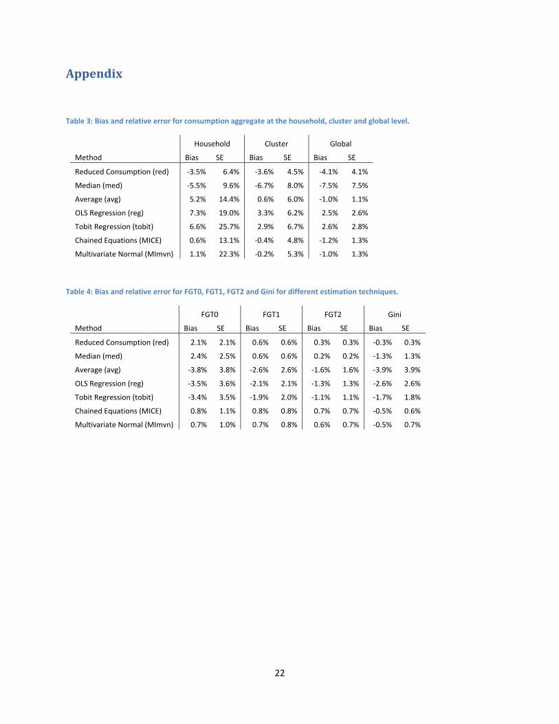
Table 3: Bias and relative error for consumption aggregate at the household, cluster and global level. 

   Household  Cluster  Global 

Method  Bias  SE  Bias  SE  Bias  SE 

Reduced Consumption (red)  ‐3.5%  6.4%  ‐3.6%  4.5%  ‐4.1%  4.1% 

Median (med)  ‐5.5%  9.6%  ‐6.7%  8.0%  ‐7.5%  7.5% 

Average (avg)  5.2%  14.4%  0.6%  6.0%  ‐1.0%  1.1% 

OLS Regression (reg)  7.3%  19.0%  3.3%  6.2%  2.5%  2.6% 

Tobit Regression (tobit)  6.6%  25.7%  2.9%  6.7%  2.6%  2.8% 

Chained Equations (MICE)  0.6%  13.1%  ‐0.4%  4.8%  ‐1.2%  1.3% 

Multivariate Normal (MImvn)  1.1%  22.3%  ‐0.2%  5.3%  ‐1.0%  1.3% 

 

Table 4: Bias and relative error for FGT0, FGT1, FGT2 and Gini for different estimation techniques. 

   FGT0  FGT1  FGT2  Gini 

Method  Bias  SE  Bias  SE  Bias  SE  Bias  SE 

Reduced Consumption (red)  2.1%  2.1%  0.6%  0.6%  0.3%  0.3%  ‐0.3%  0.3% 

Median (med)  2.4%  2.5%  0.6%  0.6%  0.2%  0.2%  ‐1.3%  1.3% 

Average (avg)  ‐3.8%  3.8%  ‐2.6%  2.6%  ‐1.6%  1.6%  ‐3.9%  3.9% 

OLS Regression (reg)  ‐3.5%  3.6%  ‐2.1%  2.1%  ‐1.3%  1.3%  ‐2.6%  2.6% 

Tobit Regression (tobit)  ‐3.4%  3.5%  ‐1.9%  2.0%  ‐1.1%  1.1%  ‐1.7%  1.8% 

Chained Equations (MICE)  0.8%  1.1%  0.8%  0.8%  0.7%  0.7%  ‐0.5%  0.6% 

Multivariate Normal (MImvn)  0.7%  1.0%  0.7%  0.8%  0.6%  0.7%  ‐0.5%  0.7% 

 

   

23  

 

Table 5: Test of Welfare Model on core consumption reporting coefficients (t‐statistics) for Mogadishu. 

Variable 

Core Food Consumption 

Core Non‐Food Consumption 

Core Food Consumption     

... 2nd Quartile  0.78 (1.17)   

... 3rd Quartile  0.09 (1.46)   

... 4th Quartile  0.52 (7.22)    

Core Non‐Food Consumption     

... 2nd Quartile    0.07 (1.11) 

... 3rd Quartile    0.12 (1.77) 

... 4th Quartile     0.42 (5.81) 

Household Size  ‐0.07 (‐8.36)  ‐0.04 (4.34) 

Household Head Education  0.16 (3.34)  0.12 (2.56) 

Dwelling Characteristics     

... Shared Apartment  0.04 (0.59)  ‐0.13 (‐2.12) 

... Separated House  ‐0.14 (‐1.13)  ‐0.19 (‐1.55) 

... Shared House  ‐0.07 (‐0.81)  ‐0.14 (‐1.52) 

Water Access 

... Piped Water  ‐0.22 (‐0.93)  ‐0.04 (‐0.19) 

... Public Tap  0.41 (2.47)  ‐0.01 (‐0.08) 

Insufficient Food in last 4 weeks  0.05 (1.49)  ‐0.05 (‐1.50) 

     

R2  0.24  0.16 

N  675  675