Forschungsinstitut zur Zukunft der ArbeitInstitute for the Study of Labor

DI

SC

US

SI

ON

P

AP

ER

S

ER

IE

S

Hours Worked in Europe and the US:New Data, New Answers

IZA DP No. 10179

August 2016

Alexander BickBettina BrüggemannNicola Fuchs-Schündeln

Hours Worked in Europe and the US: New Data, New Answers

Alexander Bick Arizona State University

Bettina Brüggemann

McMaster University

Nicola Fuchs-Schündeln

Goethe University Frankfurt, CEPR, CESifo, CFS and IZA

Discussion Paper No. 10179 August 2016

IZA

P.O. Box 7240 53072 Bonn

Germany

Phone: +49-228-3894-0 Fax: +49-228-3894-180

E-mail: iza@iza.org

Any opinions expressed here are those of the author(s) and not those of IZA. Research published in this series may include views on policy, but the institute itself takes no institutional policy positions. The IZA research network is committed to the IZA Guiding Principles of Research Integrity. The Institute for the Study of Labor (IZA) in Bonn is a local and virtual international research center and a place of communication between science, politics and business. IZA is an independent nonprofit organization supported by Deutsche Post Foundation. The center is associated with the University of Bonn and offers a stimulating research environment through its international network, workshops and conferences, data service, project support, research visits and doctoral program. IZA engages in (i) original and internationally competitive research in all fields of labor economics, (ii) development of policy concepts, and (iii) dissemination of research results and concepts to the interested public. IZA Discussion Papers often represent preliminary work and are circulated to encourage discussion. Citation of such a paper should account for its provisional character. A revised version may be available directly from the author.

IZA Discussion Paper No. 10179 August 2016

ABSTRACT

Hours Worked in Europe and the US: New Data, New Answers*

We use national labor force surveys from 1983 through 2011 to construct hours worked per person on the aggregate level and for different demographic groups for 18 European countries and the US. We find that Europeans work 19% fewer hours than US citizens. Differences in weeks worked and in the educational composition each account for one third to one half of this gap. Lower hours per person than in the US are in addition driven by lower weekly hours worked in Scandinavia and Western Europe, but by lower employment rates in Eastern and Southern Europe. JEL Classification: E24, J21, J22 Keywords: labor supply, employment, hours worked, Europe-US hours gap,

demographic structure Corresponding author: Nicola Fuchs-Schündeln Goethe University Frankfurt House of Finance 60323 Frankfurt Germany E-mail: fuchs@wiwi.uni-frankfurt.de

* This paper is based on material included in previous work of us which was circulated under the title “Labor Supply Along the Extensive and Intensive Margin: Cross-Country Facts and Time Trends by Gender”. We thank Domenico Ferraro, Berthold Herrendorf, Bart Hobijn, Roozbeh Hosseini, Richard Rogerson, Luigi Pistaferri, Valerie Ramey, B Ravikumar, Todd Schoellman, seminar participants at Aarhus University, the Federal Reserve Bank of San Francisco, Free University Berlin, and conference participants at the 2012 and 2015 Annual Meetings of the Society for Economic Dynamics, the Federal Reserve Bank of Atlanta Workshop on “Household Production and Time Allocation”, and the NBER Summer Institute Macro Perspectives Workshop 2014 and the NBER Summer Institute Conference on Research in Income and Wealth 2016 for helpful comments and suggestions. The authors gratefully acknowledge financial support from the Cluster of Excellence “Formation of Normative Orders” at Goethe University and the European Research Council under Starting Grant No. 262116. All errors are ours.

1 Introduction

An active recent literature has documented large differences in the levels and trends of aggregatehours worked per person across OECD countries, and specifically lower aggregate hours workedper person in Europe than in the US. This literature traces these lower hours in Europe back to,amongst others, labor income taxation (e.g., Prescott (2004), Rogerson (2006), Olovsson (2009),McDaniel (2011), to name a few), institutions (Alesina et al. (2005)), and social security systems(Erosa et al. (2012), Wallenius (2014), Alonso-Ortiz (2014)). One basic step to understand thecauses of the large differences in labor supply is to analyze, first, whether these differences existfor all margins of labor supply, and, second, how much they are driven by different characteristicsof the population. Are fewer Europeans working, or do they work fewer hours per work week, or dothey simply enjoy more vacation days? Are the aggregate differences driven by different sectoralcompositions across countries, different age compositions, or different educational compositions?These questions have been raised early on in Rogerson (2006) as an important avenue for advancingthe research agenda on understanding differences in hours worked across countries, but could onlybe answered to a limited extent based on existing data readily available to researchers.

This paper documents differences in hours worked per person between the US and 18 Euro-pean countries based on “new data” compiled from national labor force surveys.1 Constructinginternationally comparable hours estimates based on labor force surveys allows us to decomposedifferences in hours per person into the different components of labor supply, namely employmentrates, weeks worked per year, and weekly hours worked per employed, and to analyze to whichextent these differences are driven by different demographic and sectoral compositions. This pa-per thus provides a careful statistical decomposition of the hours differences between Europe andthe US. The resulting facts open up new avenues for research. We use three different labor forcesurveys, namely the European Labor Force Survey, the US Current Population Survey, and theGerman Microcensus, covering the time period 1983 to 2011. First, we describe how we measureemployment rates and hours worked per employed in a consistent way that leads to comparablehours worked per person estimates across countries. Next, we document that differences in ag-

gregate hours worked per person between Europe and the US are substantially larger in our data

1Ohanian and Raffo (2012) also add new evidence on the measurement of hours worked across OECD countries byconstructing hours measures at the quarterly frequency. Bick et al. (2016) measure hours worked for 81 countries in theearly 2000s focusing on the differences between low-, middle- and high-income countries rather than the differencesamong the high-income countries as we do here. Burda et al. (2008), Burda et al. (2013), Fang and McDaniel (2016),and Bridgman et al. (2016) construct cross-country hours worked measures using time-use surveys. The advantage oftime use surveys is the precise measurement of time spent over an entire work day or weekend day. The disadvantage– particularly in comparison to labor force surveys – is the much lower frequency and much smaller sample size.

1

than in the National Income and Product Accounts (NIPA) data. We analyze the reasons for thisdiscrepancy, and show implications for the measurement of labor productivity differences and forthe performance of macroeconomic models that explain the cross-country differences through tax-ation (Prescott (2004)). We then address the core question of this paper and show that differencesin weeks worked over the year account for one third to one half of the Europe-US hours gap,and a further one third to one half are explained by differences in the educational compositionacross countries. Lower hours per person in Scandinavia and Western Europe than in the US arein addition driven by lower weekly hours worked, whereas lower hours per person in Eastern andSouthern Europe are in addition driven by lower employment rates. Hence, the “new answers”we provide refer both to different evidence on aggregate hours worked per person than the oneprovided by NIPA data, and more importantly to the disaggregate evidence that cannot be obtainedfrom aggregate NIPA data. We make the data available on our webpage to the research community.

The measurement of hours worked per person, employment rates, and hours worked per em-ployed from labor force surveys is not trivial. First, the main difference between the several sur-veys, at a given point in time across countries or for a given country over time, regards the samplingof reference weeks over the year. The reference weeks range from one specific week only, to aquarter, to the sampling of all 52 weeks of the year. We document that this is not a major problemfor the consistent measurement of employment rates, but that without any further adjustment hoursworked per employed, which exhibit a fair amount of seasonality, are not measured consistently.Second, we show that even if all 52 weeks of the year are covered, vacation days are severelyunderestimated in the labor force surveys, partly because not all weeks are sampled with equalprobability. We implement a measurement strategy of hours worked per employed that is able todeal with both these issues by adjusting for vacation days, i.e. annual leave and public holidays,obtained from external data sources. It turns out that this also drastically decreases the problem ofseasonality in hours worked per employed, which is mostly driven by vacation days.

As is common practice when working with micro data sets, see e.g. the 2010 Review of Eco-nomic Dynamics special issue on “Cross Sectional Facts for Macroeconomists” (Krueger et al.(2010)), we compare our (LFS) aggregate statistics on hours worked per person with those fromthe National Income and Product Accounts (NIPA), which are provided by the OECD “NationalAccounts Database” and the Conference Board’s “Total Economy Database” (TED). For mostcountries and years, the numbers by the OECD and TED coincide, but the time-series availablefrom TED is longer than the one from the OECD. While time trends for hours are similar in LFSand NIPA data, cross-country estimates show substantial level differences between both data sets.LFS data indicate that Europeans work 19% fewer hours than Americans in the recent pre-crisis

2

years 2005-2007, while NIPA data only imply a difference of 7%. We proceed by investigatingthe sources of these large differences between LFS and NIPA data. We find that these mainlyarise from the fact that the national statistical agencies use vastly different kinds of data sets andmethods to construct hours estimates. As a consequence, the OECD itself cautions that their dataare not suitable for cross-country comparisons. In contrast, we use always the same kind of datasource, namely labor force surveys, to construct hours worked estimates, and apply exactly thesame algorithm to all data sets, thereby maximizing the comparability across countries. A furtheradvantage of the LFS data are that they are not subject to major revisions like the NIPA data.

We find that it matters for macroeconomic analyses whether one relies on LFS or NIPA data.First, we analyze implications for labor productivity differences between Europe and the US. Basedon LFS data, Europe looks with 86% of the US level closer to the US in terms of labor productivitythan with 78% based on NIPA data. This is mostly driven by the narrowing of the rather small la-bor productivity gap to the US for Western Europe by three fourths, and the large gap for SouthernEurope by one third in LFS data compared to NIPA data, while differences in productivity mea-surement between the different data sets are smaller for Eastern Europe and Scandinavia. Second,we show, relying on the work by Prescott (2004), that through the lens of a neo-classical growthmodel average tax rate differences and differences in the consumption/output ratios can accountfor 52 percent of the differences in hours worked between Europe and the US if these are measuredbased on LFS data, as opposed to more than 100 percent if they are measured by NIPA data. Thus,the explanatory power of taxes for the Europe-US hours gap is smaller when relying on LFS datathan when relying on NIPA data.

After documenting these differences in aggregate hours worked per person between LFS dataand NIPA data, we turn to the core question of the paper and provide a decomposition of hoursworked differences between Europe and the US for the recent pre-crisis years 2005 to 2007, fo-cusing on individuals aged 15 to 64. We first document that employment rates and weekly hoursworked are strongly negatively correlated across countries. By contrast, the number of work weeksduring the year is uncorrelated with both hours worked per week and employment rates. All Eu-ropean regions (Scandinavia, Western Europe, Eastern Europe, and Southern Europe) have onaverage similar hours that are 16 to 19% lower than in the US. While weeks worked are uniformlysubstantially lower in Europe than in the US, in Southern and Eastern Europe lower hours areadditionally driven by lower employment rates, but in Western Europe and Scandinavia by fewerhours worked per work week. The other component of labor supply always points in the oppositedirection: individuals in Southern and Eastern Europe work longer weekly hours than US citizens,and individuals in Scandinavia and to some extent Western Europe are more likely to be employed

3

than US citizens.Exploiting the rich micro-structure of our data, we then ask which role differences in the de-

mographic and sectoral composition between the US and different European countries play inaccounting for these differences. For instance, if older people worked on average fewer hours thanyounger people in all countries, and European countries had an on average older population, thiscould partly account for the lower hours in Europe. We investigate differences in the compositionby gender, age, education, and sectors. Any of these factors can play a role in accounting forhours differences across countries only if both the composition across countries is different and

different groups exhibit different labor supply behavior within a country. Since the age and gendercompositions across countries are in fact very similar, these two factors turn out not to play a role.By contrast, the educational compositions differ vastly across countries. In general, Europe hasa higher share of low- or medium-educated individuals and a lower share of high-educated indi-viduals than the US, especially in Eastern and Southern Europe. While weekly hours worked aresimilar for the three educational groups, employment rates increase substantially by education inall countries. Therefore, we find that differences in the educational composition between the USand the European countries are very important for understanding the hours differences via theirimpact on employment rather than on weekly hours worked. Differences in the sectoral structureturn out to matter only minimally in the statistical decomposition because differences in weeklyhours per worker between sectors are small, though larger than between education groups. Sincewe cannot assign non-working individuals to a sector, our analysis does not capture the connectionbetween sectoral shifts and employment rates, see Rogerson (2008).

Figure 1 summarizes our results: weeks worked account for between one third and one halfof the Europe-US hours differences, and the educational composition for another one third to onehalf. However, because of the strong negative cross-country correlation between employment ratesand weekly hours worked, this does not imply that these two components alone account for almostall of the differences. Lower weekly hours worked per person account for 75 and roughly 40percent of the lower hours in Scandinavia and Western Europe, respectively, than in the US, withemployment rates in Scandinavia predicting significantly higher hours there than in the US. Bycontrast, for Eastern Europe and Southern Europe (excluding Portugal), lower employment ratesaccount for roughly one half and one quarter, respectively, of the lower hours than in the US,with weekly hours worked in Eastern Europe predicting higher hours there than in the US. Lowerhours in Portugal are driven exclusively by the lower number of weeks worked and the educationalcomposition.

What do our results imply for the study of hours worked differences between Europe and the

4

Figure 1: Decomposing the Europe-US Hours Gap

1/3 to 1/21/3 to 1/2

Residual

Fewer European Lower EuropeanWeeks Worked Education Level

Scandinavia & Western Eu.: Eastern & Southern Eu.:Lower Weekly Hours Lower Employment Rates

US? We arrive at three main conclusions. First, differences in vacation days play a quantitativelysignificant role in accounting for hours worked per person differences across countries. Shouldwe think of the number of vacation days as individual choice variables, or are they rather pre-determined from an individual perspective? We document an essentially zero correlation betweenweeks worked per year and either employment rates or weekly hours worked per employed, whichcould be indicating the latter. In that case, the question arises which institutional factors driveinternational differences in vacation weeks. Moreover, to analyze the driving forces (e.g. taxation)of the hours worked decision from an individual perspective, one might want to use a model thattakes vacation days as exogenous, similarly to e.g. the model used in Kaplan (2012). In this model,involuntary unemployment (in our case vacation weeks) determines the number of weeks workedper year, and agents only choose hours worked per work week optimally. Assuming separabilityin the utility function between weeks worked and hours worked per week could lead to a zerocorrelation between weeks worked per year and either employment rates or weekly hours workedper employed. On the other hand, models with positive externalities of sharing leisure time togetheror with a (negative) signalling effect of taking annual leave could lead to multiple equilibria witheither high or low vacation days as equilibrium outcomes, and factors like taxes could serve ascoordination devices on an equilibrium.

Second, lower hours worked in Scandinavia and Western Europe are driven by lower weeklyhours per employed, and in Eastern and Southern Europe by lower employment rates. Thesefacts are robust to controlling for differences in the demographic and sectoral composition acrosscountries. What can explain these differences? Generating the negative correlation between em-

5

ployment rates and weekly hours worked in a quantitative macro model is not trivial, since mostfactors driving the individual labor supply decision tend to influence both components in the samedirection. Analyzing the sources of the negative correlation is thus a fascinating new researchagenda. In Bick and Fuchs-Schundeln (2016), we present some suggestive evidence that interna-tional differences in part-time regulation could drive the correlation.

Third, the educational composition plays a significant role in accounting for employment ratedifferences across countries. This calls for models that endogenize human capital accumulationdecisions in order to understand why college graduation rates are much higher in some countriesthan in others. What are the policies that drive different educational compositions across countries?For example, Guvenen et al. (2014), while not distinguishing between employment and hours peremployed, show that progressive taxation distorts the incentives to invest in human capital, andthat these tax differences can explain a sizable part of the differences in the Europe-US hoursper person gap for men. A further interesting new question that arises is why employment ratesuniformly increase by education, whereas hours per employed do not vary much by education.

The remainder of the paper is structured as follows: Section 2 describes the micro data setsand explains how we measure hours worked per person, employment rates, and hours worked peremployed. Section 3 compares aggregate hours worked from LFS data to those reported by NIPA.Section 4 reports the Europe-US hours difference for LFS and NIPA data, and analyzes implica-tions of using LFS data instead of NIPA data for measuring productivity differences, as well asfor models that postulate taxation as the major driving force of international hours differences.Section 5 then comes to the core analysis and decomposes aggregate hours worked differencesbetween Europe and the US in its different components, and analyzes the role of different demo-graphic subgroups. Finally, Section 6 concludes.

2 Data and Measurement

In this section, we first introduce the three labor force surveys, followed by the key questions fromthese surveys that we rely on to measure hours worked per person. Section 2.3 then presents thetwo main challenges that we face in measuring hours worked consistently across countries, namelythe sampling of reference weeks and the underreporting of vacation days. Only the former affectsthe measurement of the employment rate (by definition), but we show that this is not a majorproblem. In contrast, we we document that both of these challenges play a potentially large rolefor the measurement of hours worked per employed. Section 2.4 explains how we construct hoursworked per employed to overcome these two issues.

6

At the start of this section, let us define the main variables used throughout the paper. H

refers to average annual hours worked per person, and HE are average annual hours worked peremployed. e is the employment rate, h are hours worked per employed in a non-vacation week (aterm which we use interchangeably with weekly hours worked), and w is the average number ofnon-vacation weeks in a year (which we use interchangeably with weeks worked), such that

HE = h×w,

andH = e×HE = e×h×w.

We call the employment rate e and hours worked per employed HE the two margins of labor supply,as usual in the literature, while we talk about components when we further divide hours workedper employed into weekly hours in a non-vacation week and weeks worked.

2.1 Data Sets

We construct hours worked from three different micro data sets, namely the European Labor ForceSurvey, the Current Population Survey, and the German Microcensus.

European Labor Force Survey The European Labor Force Survey (ELFS) is a collection ofannual labor force surveys from different European countries. We use the yearly surveys, sincethe quarterly ones do not provide information on education. The ELFS covers Belgium, Denmark,France, Greece, Italy, Ireland, the Netherlands, and the UK from 1983 on, Portugal and Spainstarting in 1986, Austria, Norway, and Sweden starting in 1995, Hungary and Switzerland startingin 1996, the Czech Republic and Poland starting in 1997, and Germany starting in 2002.2 Thesample size of the ELFS varies across countries and also within a country over time, but is alwaysof considerable magnitude. The minimum annual sample size in the original data we use is 15,400for Denmark, a country with roughly 5.5 million inhabitants.

Current Population Survey For the US, we use the Current Population Survey (CPS), whichis a monthly survey of around 60,000 households. Specifically, we work with the CPS MergedOutgoing Rotation Groups data provided by the National Bureau of Economic Research (see http:

2For the Netherlands, we have information from 1983, 1985, and annually from 1987 on. The ELFS also coversFinland from 1995 on. However, the Finnish data have large numbers of missing observations for several years, whichimplies that we could only use data from 1997 to 2002 for our analysis. The ELFS covers more transition countries,which we also exclude from the analysis because of a shorter time series and a lack of information on vacation days.

7

//www.nber.org/data/morg.html). This data set includes only those interviews in which thehouseholds are asked about actual and usual hours worked, namely the fourth and eighth interviewof each household. The data cover around 300,000 individuals per year.3

German Microcensus Until Germany enters the European Labor Force Survey in 2002, weuse data from the German Microcensus. The German Microcensus covers a one percent randomsample of the population of Germany and is an administrative survey. We use the scientific usefiles, which are a 70 percent random subsample of the original sample. This leaves us with asample size of between 400,000 and 500,000 individuals per year. The scientific use files areavailable biannually from 1985 on, and annually from 1995 on. East Germans are included in thesample from 1991 onwards.

2.2 Key Survey Questions and Sample Selection

To measure employment rates and hours worked per employed person, we rely on five surveyquestions. We construct the employment rate based on the self-reported employment status in thereference week, which is usually the week prior to the interview. Employed individuals include, inaddition to employees, the self-employed and unpaid family workers. Moreover, being employeddoes not require that the individual works positive hours in the reference week. To estimate hoursworked for employed individuals, we rely on questions about actual hours worked in the main jobin the reference week, actual hours worked in additional jobs in the reference week, usual hoursworked in the main job in a working week, and reasons for having worked more or less hours thanusual in the reference week. Web Appendix Section W.1.1 discusses how we deal with missingvalues for these questions, and explains why we have to drop three country-year pairs (1983 forDenmark, 2001 for the UK, and 2005 for Spain). We include in the final sample all observations ofindividuals aged 15 to 64. Web Appendix Section W.1.1 also provides an overview of the annualfinal sample size per country, which ranges from 10,000 to 450,000 observations, with an averageof 111,000 observations.

2.3 Two Challenges

We face two key challenges when measuring hours worked per person across countries: first, thesampling of reference weeks differs across countries and within European countries over time,

3While it is well known that wages are imputed for many individuals in the CPS, this is not the case for hours, ofwhich less than 1% are imputed.

8

potentially inhibiting the comparability of measured hours. Secondly, we find that vacation daysare systematically underreported in labor force surveys.

2.3.1 Sampling of Reference Weeks

The main difference between the several surveys, at a given point in time across all countries orfor a given country over time, regards the sampling of reference weeks over the year. The CPSsamples all 12 months of the year, but uses as a reference week always the week including the12th day of a month. Therefore, most major US public holidays are not captured by the CPS (e.g.Memorial Day, 4th of July, Thanksgiving). The reference weeks in the national labor force surveysof the European countries initially fell only into country-specific periods ranging from one singlereference week to the sampling of half a year. From 2005 onwards, each week of a year is sampledin the European Labor Force Survey. Eurostat, in its efforts to harmonize the different surveysas much as possible, treated the changes in reference weeks in a two-step procedure. First, if thechange to sampling all weeks occurred in a country before 2005, the ELFS micro data reflect thisby changing from sampling only single weeks to sampling the second quarter of the calendar year(April to June) from then on until 2004. Exceptions to this rule are detailed in Web AppendixW.1.2. In a second step from 2005 onwards, when the majority of countries included in the ELFShad switched to continuous surveying, Eurostat makes all 52 weeks of the year available. The onlyexceptions to this second step rule are the UK (continuous surveying from 2008 on), Ireland (from2009 on), and Switzerland (from 2010 on).

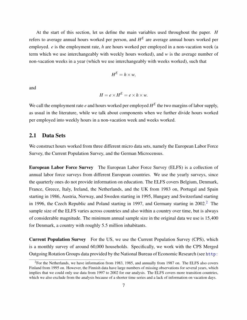
The differences in the sampling of reference weeks raise the question in how far estimates of theemployment rate and hours worked per employed are comparable across countries in a given year,and within a country over time. Since there was no change for the US, the latter question is onlyrelevant for the European countries. To give a concrete example, Figure 2 shows weekly averageactual hours worked per employed in the left panel, and weekly employment rates in the right panel,for France in 2006 by reference week. The black weeks are the weeks that were initially sampledin France until 2002 (weeks 9 to 14). The light gray weeks are weeks that include a public holiday,plus the summer vacation weeks. As one can see in the left panel of Figure 2, weekly hours workedvary substantially over the 52 weeks of the year, and are on average significantly lower in vacationweeks. The sampling of reference weeks thus matters for the aggregate: the grey horizontal barindicates average weekly hours worked over all 52 weeks, while the black horizontal bar indicatesaverage weekly hours worked over the initially sampled black weeks: the difference amounts to 3.1weekly hours. By contrast, the right panel of Figure 2 shows that the employment rate is roughlyconstant over all 52 weeks of the year.

9

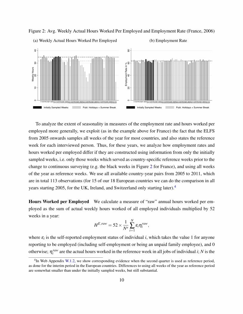
Figure 2: Avg. Weekly Actual Hours Worked Per Employed and Employment Rate (France, 2006)

(a) Weekly Actual Hours Worked Per Employed0

1020

3040

Wee

kly

Hou

rs

1 2 3 4 5 6 7 8 9 10 11 12 13 14 15 16 17 18 19 20 21 22 23 24 25 26 27 28 29 30 31 32 33 34 35 36 37 38 39 40 41 42 43 44 45 46 47 48 49 50 51 52

Initially Sampled Weeks Publ. Holidays + Summer Break

(b) Employment Rate

020

4060

80Em

ploy

men

t Rat

e in

%

1 2 3 4 5 6 7 8 9 10 11 12 13 14 15 16 17 18 19 20 21 22 23 24 25 26 27 28 29 30 31 32 33 34 35 36 37 38 39 40 41 42 43 44 45 46 47 48 49 50 51 52

Initially Sampled Weeks Publ. Holidays + Summer Break

To analyze the extent of seasonality in measures of the employment rate and hours worked peremployed more generally, we exploit (as in the example above for France) the fact that the ELFSfrom 2005 onwards samples all weeks of the year for most countries, and also states the referenceweek for each interviewed person. Thus, for these years, we analyze how employment rates andhours worked per employed differ if they are constructed using information from only the initiallysampled weeks, i.e. only those weeks which served as country-specific reference weeks prior to thechange to continuous surveying (e.g. the black weeks in Figure 2 for France), and using all weeksof the year as reference weeks. We use all available country-year pairs from 2005 to 2011, whichare in total 113 observations (for 15 of our 18 European countries we can do the comparison in allyears starting 2005, for the UK, Ireland, and Switzerland only starting later).4

Hours Worked per Employed We calculate a measure of “raw” annual hours worked per em-ployed as the sum of actual weekly hours worked of all employed individuals multiplied by 52weeks in a year:

HE,raw = 52× 1Ne

N

∑i=1

εiηrawi ,

where εi is the self-reported employment status of individual i, which takes the value 1 for anyonereporting to be employed (including self-employment or being an unpaid family employee), and 0otherwise; ηraw

i are the actual hours worked in the reference week in all jobs of individual i; N is the

4In Web Appendix W.1.2, we show corresponding evidence when the second quarter is used as reference period,as done for the interim period in the European countries. Differences to using all weeks of the year as reference periodare somewhat smaller than under the initially sampled weeks, but still substantial.

10

total number of individuals; and Ne is the number of employed individuals, i.e. Ne = ∑Ni=1 εi. All

measures are calculated using the individual survey weights, which we omit for ease of exposition.Table 1 shows in the first row the absolute percentage deviation of annual hours worked per em-

ployed (aged 15 to 64) when using only the initially sampled reference weeks from using all weeksof a year, which amounts on average to 3.5%. At the 90th percentile, the deviation already reaches7.0%, with a maximum deviation of 12.6% in Sweden for the year 2008. Thus, the sampling of thereference weeks matters substantially for the measurement of hours worked per employed. Withonly few exceptions, the hours when only specific survey weeks are sampled are larger than whenall weeks of the year are sampled.5

Employment Rate The employment rate (e) is simply given by the number of employed indi-viduals divided by all individuals in the sample

e =Ne

N. (1)

Equation (1) is the employment to population ratio for the population 15-64, but we henceforthrefer to it as the employment rate.6 The second row of Table 1 shows that the employment rateexhibits significantly less seasonality than the raw hours worked per employed measure. The aver-age absolute percentage point deviation between constructing the employment rate only based onspecific survey weeks relative to the entire year amounts to only 0.7 percentage points. At the 90thpercentiles, the difference is still relatively small with 1.3 percentage points. Moreover, employ-ment rates are not systematically higher (or lower) if only specific weeks are sampled than whenthe entire year is sampled. There are only a few observations that are worrisome with deviationsover 5 percentage points. The five country-year observations above the 95th percentile come fromGermany (four times) and Belgium. Both countries used only one specific week as reference week(Germany until 2004, Belgium until 1998), suggesting that the corresponding time-series of theemployment rates have to be used with some caution.

5This is the case for all countries in all but at most one year. The only exception are the Netherlands, where hoursare lower in the initially sampled weeks, with the exception of two years.

6Web Appendix Section W.1.3 reports two alternative measures of the employment rate. The first alternativemeasure relies on defining employment based on usually working positive hours. This leaves the employment ratevirtually unchanged. The second alternative measure involves a different definition of employment for women onmaternity leave. This has only a modest impact on female employment rates, and is far too small to drive internationaldifferences in female employment rates. Note that by construction, hours worked per person remain always the sameno matter what definition is used for the employment rate, because an increase (decrease) in the alternative employmentrate relative to our baseline definition is always offset by a decrease (increase) in the corresponding measure of hoursworked per employed.

11

Table 1: Absolute %-Deviations∗ of HE,raw, e, and HE Using Only Initially Sampled Weeks fromUsing All 52 Reference Weeks

Mean 75th 90th 95th 99th Max

HE,raw 3.5 4.7 7.0 7.9 11.4 12.6e 0.7 0.8 1.3 1.9 5.3 5.9HE 0.8 1.1 1.5 2.1 3.7 5.0

Note: For HE,raw and HE we report deviations in percentages, whereas for e we use percentage points.

2.3.2 Underreporting of Vacation Weeks

For most European countries, all weeks of the year are sampled from 2005 onwards. If each weekwould be sampled with equal probability and cover a representative sample of the population weekby week (rather than only over the entire year), then average vacation weeks should be capturedaccurately in the labor force surveys. Calculating the average number of vacation weeks from themicro data yields an average of 3.3 “self-reported” vacation weeks, where we define vacation asthe sum of public holidays and annual leave.7 Given that public holidays alone in all countriessum up to 1.5 to 2.5 weeks, these self-reported weeks of annual leave and public holidays seemimplausibly low. In fact, based on external data sources, the average weeks of vacation over thesame time period for our sample of European countries amount to 6.8 weeks per year.8

To get a better understanding of the sources of this discrepancy, we investigate in more detailthe case of Germany, which features the largest difference among all countries, amounting to 5.5weeks. While we provide all details in Web Appendix Section W.2.2, our results of this analysiscan be summarized as follows. First, using the German Socio-Economic Panel, Schnitzlein (2011)reports that on average 3 of the average 31 entitled days of annual leave per year go unused. Thus,the underusage of entitled leave can explain only a very small portion of the discrepancy of 5.5weeks between self-reports and official vacation days. Second, not all weeks are sampled with thesame probability in the Microcensus, see Figure W.1 in Web Appendix Section W.2.2. For exam-ple, the reference week which contains Christmas day is on average sampled with a probability of1.3%, significantly below the 1.9% that would be implied by equal sampling. Third, the GermanStatistical Office also has some evidence that respondents might dislike using a vacation week as a

7Table W.10 in Web Appendix W.2.2 reports the results for each country as well as the description of how weconstruct the self-reported vacation weeks.

8Web Appendix W.2.1 lists the external data sources and explains further assumptions in the construction of thenumber of vacation weeks. It also shows that the time series variation in vacation weeks within each country is small,with the notable exception of Denmark. For the US, the discrepancy between self-reported and external vacationweeks is somewhat smaller but still substantial, with 1.4 vs. 3.5 weeks. We expect a discrepancy for the US, sinceweeks with major public holidays are not sampled.

12

reference week, either because they are too busy the first week after a vacation to fill out the ques-tionnaire, or because they perceive it as “inappropriate” to use a vacation week as reference weekwhen in fact they are generally hard working. Summarizing, at least for Germany there exists evi-dence of underreporting of days of annual leave and public holidays in the Microcensus even afterthe introduction of continuous sampling over the entire year. It seems at least not implausible thatthese factors can explain the discrepancies between the self-reported and external vacation weeksfor the remaining countries as well. Therefore, it is important to adjust hours worked per em-ployed for vacation using external data in the European countries even when analyzing the recentcross-section from 2005 onwards.

2.4 Measurement of Hours Worked per Employed

As documented so far, the raw measure of hours worked per employed suffers from two weak-nesses: first, seasonality in hours worked per employed impedes the comparability of hours workedacross countries and within European countries over time because of differences in the sampledreference weeks; secondly, vacation weeks are underreported in the labor force surveys even if allweeks of a year are sampled. We therefore apply the following adjustment to construct a measureof hours worked per employed that overcomes both weaknesses: we first obtain individual hoursworked in a non-vacation week, i.e. a typical work week without a reduction in work time becauseof a public holiday or annual leave, and then require consistency of annual leave and public holi-days in the micro data with the country-wide average. This closely follows the procedure in Pilat(2003).

To calculate hours worked in a non-vacation week ηi for each employed individual, we use as abaseline actual hours worked in all jobs in the reference week. However, if a respondent indicatesthat he/she worked less hours than usual in the main job in the reference week, and states as themain reason for doing so public holidays or annual leave, we replace weekly hours by usual hoursin the main job plus actual hours worked in all additional jobs.9 Thus,

ηi =

usual hours in main job if actual hours in main job<usual hours in main job

+ actual hours in all additional jobs because of annual leave or public holiday

actual hours in all jobs ηrawi otherwise.

9Note that respondents can only indicate one reason for working different hours than usual, and for additional jobswe do not have information on usual hours. In Web Appendix W.1.4 we discuss some differences between the CPSand ELFS questionnaire regarding the construction of our hours measure, which however have virtually no impact onthe statistics presented in the paper.

13

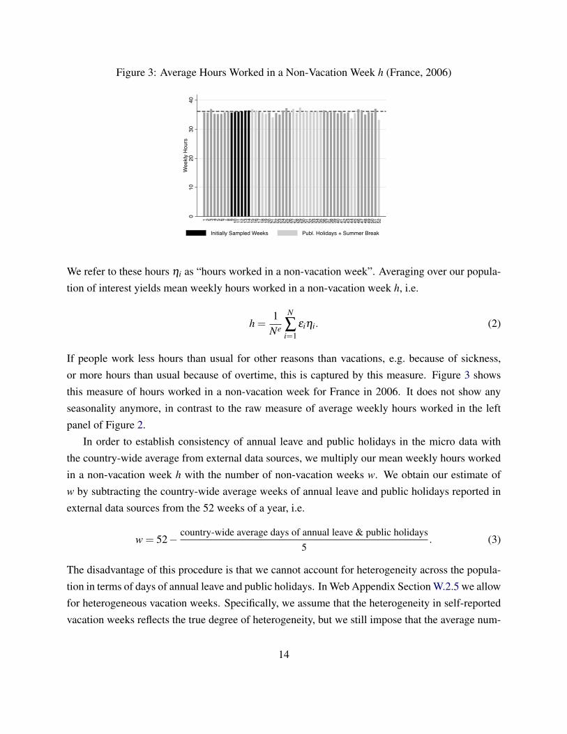
Figure 3: Average Hours Worked in a Non-Vacation Week h (France, 2006)

010

2030

40W

eekl

y H

ours

1 2 3 4 5 6 7 8 9 10 11 12 13 14 15 16 17 18 19 20 21 22 23 24 25 26 27 28 29 30 31 32 33 34 35 36 37 38 39 40 41 42 43 44 45 46 47 48 49 50 51 52

Initially Sampled Weeks Publ. Holidays + Summer Break

We refer to these hours ηi as “hours worked in a non-vacation week”. Averaging over our popula-tion of interest yields mean weekly hours worked in a non-vacation week h, i.e.

h =1

Ne

N

∑i=1

εiηi. (2)

If people work less hours than usual for other reasons than vacations, e.g. because of sickness,or more hours than usual because of overtime, this is captured by this measure. Figure 3 showsthis measure of hours worked in a non-vacation week for France in 2006. It does not show anyseasonality anymore, in contrast to the raw measure of average weekly hours worked in the leftpanel of Figure 2.

In order to establish consistency of annual leave and public holidays in the micro data withthe country-wide average from external data sources, we multiply our mean weekly hours workedin a non-vacation week h with the number of non-vacation weeks w. We obtain our estimate ofw by subtracting the country-wide average weeks of annual leave and public holidays reported inexternal data sources from the 52 weeks of a year, i.e.

w = 52− country-wide average days of annual leave & public holidays5

. (3)

The disadvantage of this procedure is that we cannot account for heterogeneity across the popula-tion in terms of days of annual leave and public holidays. In Web Appendix Section W.2.5 we allowfor heterogeneous vacation weeks. Specifically, we assume that the heterogeneity in self-reportedvacation weeks reflects the true degree of heterogeneity, but we still impose that the average num-

14

ber of vacation weeks corresponds to the one from external sources. The implied differences to thecase of homogeneous vacation weeks are small.

The third row of Table 1 shows the deviation of the annual hours worked per employed measure(HE = h×w) if only the initially sampled survey weeks are used as reference weeks, compared toall weeks of the year. While for the “raw” measure of hours worked per employed in the first rowthe mean absolute percentage deviation amounts to 3.5%, the mean absolute percentage deviationof our measure of hours worked per employed is with 0.8% substantially smaller. Thus, externallyadjusting for vacation is successful in insuring comparability of the data over time. Only at the topend of the distribution we still see a non-negligible effect of the sampling of the reference weeks.The three countries with deviations in the top five percent are Belgium, Norway, and Poland.

Finally, while we document the need to adjust for hours lost due to public holidays and annualleave, the same could in principal apply to working less hours than usual because of sick leave orother reasons, and also to working more hours than usual (overtime and additional jobs). Thereare two dimensions to this issue. First, in how far do such differences between usual and actualhours vary with the set of reference weeks available? In Web Appendix Section W.3, we provideevidence that none of the other reasons for working more or less time than usual vary with the setof reference weeks, thus seasonality is not important for them. Second, is there systematic under-or overreporting of these categories? We collect some suggestive evidence for sick days for asubset of countries and years. Comparing sick days from external data sources to the reported sickdays in our data, we find that the self-reported number of sick days are smaller than sick days fromexternal data sources, a similar finding as the one for vacation days. However, the discrepancyis on average smaller than for vacation days and public holidays, with on average 1.2 weeks inEurope and 0.3 weeks in the US, see Web Appendix Section W.3.

3 Comparing LFS Hours with NIPA Hours

We use data from labor force surveys to analyze the role of different margins and the demographiccomposition for international hours worked differences. This raises the natural question how theaggregate hours constructed from labor force surveys (henceforth referred to as LFS hours) com-pare with hours in the National Income and Product Accounts (NIPA). In this section, we showthat differences between aggregate hours in LFS and NIPA are large, and argue that they are notdriven by conceptual differences between both, but rather by the use of vastly different kinds ofdata sources and methods in the construction of NIPA data.

We rely on two commonly used sources for international NIPA data. The OECD gathers in

15

its “National Accounts Database” (stats.oecd.org) total hours worked and total employment atan annual frequency provided by the national statistical agencies. The measurement of both vari-ables follows the most recent System of National Accounts (SNA) guidelines, see Chapter 19 inEuropean Commission et al. (2009) and Chapter 11 in Eurostat (2013). Secondly, the ConferenceBoard provides total hours worked and total employment in its “Total Economy Database” (TED)(http://www.conference-board.org/data/economydatabase). Both OECD and TED datahave been widely used in the literature studying driving forces and implications of aggregate hoursdifferences across countries. Since for the majority of countries and years in our sample the datafrom the OECD and the TED are exactly the same, we focus on the comparison of LFS data toNIPA data obtained from the OECD’s “National Accounts Database”. Note that the five mainpapers explaining hours worked differences between Europe and the US with quantitative macromodels (Prescott (2004), Rogerson (2006), Ohanian et al. (2008), McDaniel (2011), and Ragan(2013)) all use slightly different approaches to calculate hours worked per person.10 With the ex-ception of McDaniel (2011), these papers multiply a measure of total hours worked per employed,either from the OECD or from the TED, with variants of the civilian employment rate based onOECD data (see Web Appendix Section W.4.4 and Bick et al. (2016) for details). We opt to workwith NIPA data, since employment then refers to total employment in both hours worked per em-ployed and the employment rate, thus canceling out when calculating hours worked per person.

The main conceptual difference between LFS and NIPA estimates of employment and hoursworked relates to the covered population. LFS data cover civilian, non-institutionalized residentsof a country aged 15 and older. NIPA data deviate from this in two dimensions. Figure 4 illustratesthese differences in the coverage. First, employment and hours estimates in NIPA are based on thedomestic concept and constructed such that the labor inputs are consistent with the measurementof gross domestic output (GDP), while LFS follow the national concept based on residence of theworker. Thus, NIPA exclude employment and hours worked of civilian, non-institutionalized res-idents who work in a foreign country (e.g., from the German perspective a resident of Germanyworking in Switzerland). On the other hand, NIPA data include domestic employment and hoursworked even if they originate from individuals residing in a foreign country (e.g., from the Ger-man perspective also hours worked by residents of Switzerland working in Germany). In addition,NIPA data do not restrict the covered population to the non-institutionalized civilians aged 15 and

10The OECD also provides information on average annual hours actually worked per worker in its “LabourDatabase” under the category “Labour Force Statistics” . For most countries in our sample and for most years, thisestimate is equal to total hours worked divided by total employment from the “National Account Database”. Moreover,the OECD provides under the category “Labour Force Statistics” two different measures of civilian employment, oneunder the “Annual Labor Force Statistics”, another one under “LFS by sex and age”, which generally do not coincide,although the differences are usually small.

16

Figure 4: Population Coverage in NIPA and LFS

Civilian residents aged 15+ working domestically

NIPA LFS

Foreign residents working domestically Armed Forces Further groups - Aged 0-14 - Institutionalized - Diplomats - …

Civilian residents aged 15+ working abroad

NIPA: country-specific data sources and methods

older, but include employment and hours worked from all individuals contributing to GDP: non-civilians (members of the armed forces) and further groups, including individuals younger than 15,institutionalized individuals (e.g., prisoners), and others as e.g., diplomats (e.g., from the Germanperspective the German ambassador in the US) or students abroad. Secondly, besides these differ-ences related to the covered population, LFS and NIPA data on hours worked and employment candiffer for the same covered population (i.e. civilian, non-institutionalized residents of a countryaged 15 and older that do not work in a foreign country; the intersection in Figure 4). The nationalstatistical agencies use very different country-specific kinds of data sources and methods in theconstruction of NIPA data (see Web Appendix W.4.1), which makes the cross-country comparisonof hours worked difficult, despite the efforts to harmonize measurement through the Systems ofNational Accounts, see also Fleck (2009). These data sources comprise administrative data, socialsecurity data, employer surveys, labor force surveys, census data, etc. In fact, the OECD remarkson its website that “The [hours worked] data are intended for comparisons of trends over time;they are unsuitable for comparisons of the level of average annual hours of work for a given year,because of differences in their sources” and recommends using employment rates based on laborforce surveys for cross-country comparisons: “National Labor Force Surveys are the best way tocapture unemployment and employment according to the ILO guidelines that define the criteriafor a person to be considered as unemployed or employed... data from LFS make internationalcomparisons easier compared to a mixture of survey and registration data ... ”.11

Having discussed the conceptual differences between LFS and NIPA hours, we now turn toquantifying the observed differences. As commonly done in cross-country comparisons, we focus

11Both quotes are from the OECD’s website: http://stats.oecd.

org/Index.aspx?DataSetCode=ANHRS and http://www.oecd.org/els/emp/

basicstatisticalconceptsemploymentunemploymentandactivityinlabourforcesurveys.htm. Theywere retrieved on August 12, 2016.

17

Figure 5: Percentage Deviations of Hours Worked and Employment in NIPA from LFS

(a) Hours Worked per Person-1

0-5

05

1015

20%

Dev

iatio

n of

NIP

A fr

om L

FS H

ours

per

Per

son

US AT BE CH CZ DE DK ES FR GR HU IE IT NL NO PL PT SE UK

Hours per Person

(b) Empl. Rate and Hours Worked per Employed

-10

-7.5

-5-2

.50

2.5

57.

510

12.5

% D

evia

tion

of N

IPA

from

LFS

US AT BE CH CZ DE DK ES FR GR HU IE IT NL NO PL PT SE UK

Employment Rate Hours per Employed

on the comparison of hours per person rather than total hours worked. We obtain a NIPA measureof hours worked per person by dividing NIPA total hours by the population aged 15 to 64 obtainedfrom the OECD’s “Annual Labour Force Statistics”.12 For the LFS data, we divide LFS hours bythe population aged 15 to 64 directly taken from the LFS, i.e. by the civilian, non-institutionalizedpopulation aged 15 to 64.

Figure 5a shows the average country-specific percentage deviation of NIPA estimates for hoursworked per person from LFS estimates for the recent pre-crisis years 2005 to 2007. The NIPAestimate is larger than the LFS estimate for the majority of countries (on average by 7.2%). Onlyin 5 out of 19 countries are the NIPA estimates below the LFS estimates (on average by -4.2%).

To gain a better understanding of the sources of these differences, we turn to the two mar-gins of labor supply. Figure 5b shows for the employment rate (black bars) and hours worked peremployed (grey bars) the percentage deviations of the NIPA estimate from the respective LFS es-timate. The NIPA employment rate estimate exceeds the LFS estimate in the majority of countries(on average by 4.0%, or 2.2 percentage points). Italy stands out with the difference exceeding10%, followed by Switzerland, Germany, and Spain with differences of over 5%. In 5 countriesis the NIPA employment rate lower than the LFS one, however only in the US and Poland in aneconomically significant way. Relative to the employment rate differences, the hours per employeddifferences are less systematic. In fact, the NIPA hours per employed estimate is lower than the

12These data can be found in the OECD’s “Labour Database” under the category “Labour Force Statistics”, andcover all residents of a country. The OECD National Accounts data do not provide any population figures brokendown by age groups. Population figures are generally only available for the national concept and including everyoneindependent of status (civilian vs. non-civilian, institutionalized vs. non-institutionalized).

18

LFS estimate for 10 countries (on average by -4.1%) and higher in 9 countries (on average by7.8%). There is also no systematic relationship between NIPA-LFS differences for the employ-ment rate and hours per employed. The correlation between the two differences is -0.13.

What drives these differences between NIPA and LFS estimates? We can partially analyze thisfor employment rates, based on additional data from the OECD’s “National Accounts Database”and “Annual Labor Force Statistics”. In Web Appendix W.4.2, we provide a detailed discussionof this investigation. In a nutshell, differences in employment stemming from the location ofemployment, i.e. the net difference in domestic residents working abroad and foreign residentsworking domestically, are for most countries negligible, with the exceptions of Switzerland andHungary. The exclusion of non-civilian employment, i.e. the armed forces, in the LFS is alsoessentially irrelevant for the differences (even in the US). The “further groups” in Figure 4 aregenerally too small to rationalize the remaining employment rate differences. This leaves as themajor driving force of the differences the use of different kinds of data sets and different methodsby the national statistical agencies.

Unfortunately, for hours worked per employed we cannot conduct such a comparison, sincethe OECD does not provide hours for the armed forces or the total population using the nationalconcept as for employment. The documentations provided by the national statistical agencies onhow hours are estimated are also not helpful in getting quick insights into the differences. WebAppendix W.4.1 shows in the left column the country-specific main data sources to construct em-ployment rates, and in the right column the main sources to construct hours worked per employed.Both differ widely across countries. For Germany, for example, in addition to the two main datasources mentioned in the table, the hours estimate relies on 60 different data sets and is estimatedwith various econometric models. This makes it impossible to investigate what exactly generatesthe differences relative to the German LFS data.

For the US in turn, it is well known and documented that the hours estimates based on the CPSdiffer from NIPA estimates, for which the Current Employment Statistics (CES) by the BLS are themain data source. Through 2005, the CES data cover only production workers in goods-producingindustries, and non-supervisory workers in services-providing industries, both within the privatenon-agricultural sector. These groups tend to have lower hours than the non-covered groups. Fornon-production and supervisory workers, hours are imputed based on data from 1978 assumingthe same trends as for the covered groups, though data based on the CPS are not supporting thecommon trend assumption, see Eldridge et al. (2004). Only from 2006 onwards, all employees arecovered. For all years, the NIPA estimate is supplemented by hours of self-employed and unpaidfamily workers from the CPS. Our data from the CPS in turn always cover all employees, next to

19

the self-employed and unpaid family workers. Another difference is that the CES measure hoursper job, while the CPS measures hours per person in all jobs. In the presence of multiple jobholders (about 5 to 6% of the population), the CES estimate will therefore be downward biased.Next, the CES measure hours paid, which are adjusted for paid vacations but not off-the-clockwork, whereas the CPS measures hours worked. Last, there are differences in the reference period.The CES report hours for the pay period that includes the 12th of a month and can be weekly,biweekly or monthly, whereas the CPS reports hours for the week which includes the 12th of amonth. Frazis and Stewart (2010) conclude that these differences can largely account for the leveldifferences between CPS and NIPA hours estimates. They further document that hours in theCPS line up well with those from the American Time Use Survey, disproving an often mentionedcriticism that hours in labor force surveys are overreported. Ramey (2012) shows that the datasource matters for the measurement of the trend and cyclical behavior of labor productivity, andsuggests the use of the CPS hours series.

While we have documented that in terms of levels NIPA and LFS hours estimates differ sub-stantially for most countries, the time trends are much more in line with each other, although thereare some exceptions. Figures W.22 to W.40 in Web Appendix W.4.3 show for each country thetime-series of hours per person, employment rates and hours per employed based on LFS andNIPA data from the OECD, and in addition from TED. As mentioned before, for most years andcountries, the OECD and TED data series coincide, while the TED data usually go further back intime than the OECD data (and the LFS data).

Which data source is better suited for international comparisons remains an open question.We do not want to discount by any means the important and careful work by the national statis-tical agencies to measure labor inputs and output in each country in a consistent way. We wantto emphasize however that the advantage of the labor force surveys is that we use a consistentdata source and apply exactly the same methodology across countries, while NIPA estimates differsubstantially in country-specific ways in both the kind of data sources used and the methodologyapplied. On top of this, NIPA data both by the OECD and the TED are subject to substantialrevisions over time that also apply to previous years, which affect quantitative statements dramat-ically, see Web Appendix W.4.4 and Bick et al. (2016). As argued in Johnson et al. (2013) andPinkovskiy and Sala-i-Martin (2016) for data revisions in the Penn World Tables, it is not clearthat these revisions lead to improvements of the data, and the opposite might actually be true. Asmentioned above, the OECD itself cautions that their data are not intended for cross-country com-parisons of levels, and suggests the use of labor force surveys instead. Before exploiting the keyadvantage of our data, namely the possibility to analyze the importance of different components

20

Table 2: Avg. Hours Worked per Person Relative to the US (in %) - Summary Statistics 2005-2007

Country LFS NIPA

Mean −19.0 −7.1Standard Deviation 6.6 9.3Min Abs Deviation 5.1 3.3Max Abs Deviation 30.2 23.6

and the demographic composition for total hours worked per person, we discuss in the next sectionthe quantitative differences in the estimates of the Europe-US hours gap in NIPA and LFS data.

4 Hours Differences between Europe and the US: Measure-ment and Implications

In this section, we first document hours worked per person differences between Europe and theUS in the recent pre-crisis period 2005 to 2007 based on LFS data and NIPA data. We showthat the differences are much larger based on LFS data. This is driven by both higher hours forthe US and on average lower hours for Europe in LFS data. We then analyze two implicationsof the different measurements of the Europe-US hours gap, namely first for the measurement ofproductivity differences, and secondly for the analysis of models that postulate taxation as themajor driving force of international hours differences.

4.1 Documenting Hours Differences between Europe and the US

Table 2 reports the difference in average hours worked per person between the 18 European samplecountries and the US in LFS and NIPA data in the period 2005 to 2007. Based on LFS dataEuropeans work on average 19% fewer hours than US citizens, compared to only 7% based onNIPA data.13 Thus, the differences between Europe and the US are less than half as large inNIPA data than in LFS data, a stunning difference. The larger differences between Europeanand US hours in LFS data relative to NIPA data are driven by both the higher hours worked perperson estimates for the US in LFS data and the lower ones for Europe. US hours worked perperson are with 1397 hours in LFS data 120 hours higher than in NIPA data with 1277 hours. By

13If we use the average vacation weeks from LFS data rather than from external data sources for our adjustment,the Europe-US hours gap is only mildly reduced to -16.1%. The population weighted Europe-US hours gap is -13.5%for LFS data and -6.7% for NIPA data.

21

Figure 6: Average Hours Worked per Person Relative to the US (in %), 1983-2011

7 8 9 11 14 16 18

-30

-25

-20

-15

-10

-50

1983 1987 1991 1995 1999 2003 2007 2011Year

LFS OECD TED

Note: The vertical lines indicate the years in which new countries enter the LFS sample, and the numbers next tothem indicate the number of European countries in the sample from then on.

contrast, average hours worked per person over all European countries are with 1132 hours 55hours lower in LFS data than in NIPA data. Therefore, around two thirds of the larger Europe-UShours difference in LFS data than in NIPA data come from higher US hours, and around one thirdfrom lower European hours. Finally, in terms of the cross-sectional variation within Europe, ourdata display a smaller standard deviation.

One might wonder whether the large discrepancies in the Europe-US hours difference betweenLFS data and NIPA data are an artifact of the pre-crisis cross-section, or have been present forsome time. Figure 6 shows the average Europe-US hours difference in LFS data vs. OECD andTED data starting in the earliest sample year from the LFS data set, namely 1983.14 The verticallines indicate the years in which new countries enter the LFS sample, and the numbers next tothem indicate the number of European countries in the sample from then on. Since the numberof European sample countries expands over time, the graph does not give a meaningful indicationof the time-series development of the overall Europe-US hours difference before 1997. However,in any given year the sample countries are always the same in all three data sources. LFS dataalways indicate substantially larger Europe-US differences than either OECD or TED data, withthe average absolute gap between the LFS and the OECD (TED) difference amounting to 11 (10)percentage points after 1997.

14The Europe-US hours gap is slightly larger for TED data as they feature a slightly larger hours per person estimatefor the US, while TED and OECD hours per person estimates for Europe are basically the same.

22

Figure 7: Average Hours Worked per Person Relative to the US by Country, 2005-2007

-30

-20

-10

010

Hou

rs p

er P

erso

n R

elat

ive

to th

e U

S (in

%)

CH PT CZ DK AT GR IE UK SE NO ES NL HU DE PL BE FR IT

LFS NIPAMean Mean

Note that Prescott (2004), as well as other papers from this literature like Ohanian et al. (2008),Rogerson (2006), and McDaniel (2011), all rely on data from either OECD or TED using threedifferent methods to measure hours worked per person, but find Europe-US hours gaps that aresimilar to the ones we document for LFS data. The reason is that both OECD and TED substantiallyrevised their measures of hours worked per employed in new releases over the years, each time alsoaffecting all previous years in the data series. Relying exactly on the formula and the data releasesused by Ohanian et al. (2008), we find a Europe-US hours gap of 17.6% for 2003 (the latestavailable year in Ohanian et al. (2008)). Using exactly the same formula and same data sources, butworking with the most recent releases from May 2016 (TED) and August 2016 (OECD), insteadgives a gap of 11.0% for the year 2003.15 Web Appendix Section W.4.4 and Bick et al. (2016) givefurther evidence of the importance of data revisions in OECD and TED data.

Figure 7 plots hours worked per person differences (averaged over the years 2005 to 2007)between each European country and the US for the NIPA data (from the OECD) and LFS data,sorting the countries by decreasing difference to the US based on LFS data. With the exceptionsof Switzerland, Portugal, Greece, and Ireland for NIPA data, hours worked per person in Europeare always lower than in the US. Furthermore, LFS data always predict a larger negative differenceto the US than NIPA data. The smallest difference to US hours (in absolute value) in LFS dataamounts to -5.1% for Switzerland, where NIPA reports higher hours than in the US by 8.6%. Thelargest difference to US hours in LFS data comes from Italy with -30%, where NIPA indicates

15Note that the three Eastern European countries in our sample are excluded from this comparison as they are notin the Ohanian et al. (2008) data set.

23

a difference of only -7.8%. Italy is the country on which the two data sources deviate most (22percentage points), followed by Greece, Ireland, and Portugal. The smallest discrepancies arisefor Belgium, Denmark, and Germany, with less than 5 percentage points. Still, the ranking ofthe countries is mostly preserved between both data sets: the correlation between the LFS hoursworked per person measure and the NIPA measure is 0.74.

4.2 Productivity Differences between Europe and the US

Hours worked are a crucial input into the measurement of labor productivity, i.e. GDP dividedby total hours worked. NIPA hours are generally the appropriate measure to calculate labor pro-ductivity because they are constructed specifically such that the labor inputs are consistent withthe measurement of GDP. We (and the OECD itself) however argue above that LFS data might bebetter suited for international comparisons, since they are built using the same sources and method-ology across countries. Given that LFS data provide different estimates of total hours than NIPAdata, LFS data also lead to different conclusions regarding productivity differences between Eu-rope and the US. Taking a measure of total GDP from the Penn World Tables (Y Total

PWT ), and defining

total hours worked as HTotal , we can define labor productivity in country c as LPci =

Y Total,cPWT

HTotal,ci

with

i ={NIPA, LFS}. Labor productivity relative to the US is then defined as LPci

LPUSi

=Y Total,c

PWT /Y Total,USPWT

HTotal,ci /HTotal,US

i.

The larger the ratio between a country’s hours and US hours in LFS data relative to NIPA data, thesmaller is the labor productivity gap between this country and the US based on LFS data relativeto NIPA data.

Table 3 calculates average GDP per hour worked over the years 2005 to 2007. In the firstcolumn, total hours worked are constructed from LFS data, in the second column they are takenfrom NIPA. GDP comes from the Penn World Tables Version 9.0, and is defined as the output-sidereal GDP at chained PPP in 2011 US-Dollar (rgd po; see Feenstra et al. (2015)). GDP per hourworked in the US is normalized to 100 in both columns. The following rows then show GDPper hour worked in each of the European countries relative to the US. Total hours worked in theUS are 10% higher in LFS data than in NIPA data, which leads to a lower estimate of GDP perhour worked in the US of $49.7 (in 2011 US-Dollar) based on LFS data compared to $57.9 basedon NIPA data. We group the European countries into four regions, namely Scandinavia, WesternEurope, Eastern Europe, and Southern Europe.

Given the larger hours difference between Europe and the US in LFS data than in NIPA data,we find smaller productivity differences overall between Europe and the US based on LFS data.While based on NIPA data Europe features 78% of the labor productivity of the US, based on

24

Table 3: GDP per Hour Worked Relative to the US (in %)

Country LFS NIPA

US 100.0 100.0

Europe 86.4 78.0

Denmark 88.3 86.9Norway 172.0 161.8Sweden 92.0 84.8

Mean 117.4 111.2

Austria 85.2 78.0Belgium 91.4 88.7France 98.3 92.5Germany 97.0 94.2Ireland 114.8 96.9Netherlands 107.2 98.8Switzerland 94.9 83.8United Kingdom 92.0 80.3

Mean 97.6 89.1

Czech Republic 50.2 47.6Hungary 45.2 37.8Poland 40.1 34.4

Mean 45.1 39.9

Greece 64.0 51.3Italy 93.7 74.0Portugal 50.6 44.3Spain 78.2 68.5

Mean 71.6 59.5

LFS data Europe’s labor productivity amounts on average to 86% of the US one. Quantitatively,the differences across data sets are largest in absolute terms for Southern Europe: based on NIPAdata, Southern Europe exhibits only 60% of the labor productivity of the US, while based onLFS data Southern Europe’s labor productivity amounts to 72% of the US one. Put differently,the productivity gap is reduced by nearly one third relative to NIPA data. The results for Italyare particular striking, where the labor productivity gap nearly disappears for LFS data. WesternEuropean labor productivity is at 89% of the US productivity based on NIPA data, but comesvery close to the US level with 98% based on LFS data. Hence, for Western Europe we see the

25

largest reduction in relative terms of the labor productivity gap (by three fourths). Differencesin productivity measurement between the different data sets are smallest for Eastern Europe andScandinavia. In Eastern Europe, labor productivity is with 45% of the US level still higher in LFSdata than with 40% in NIPA data. Because of the extraordinary high labor productivity in Norway,on average Scandinavian labor productivity surpasses the one in the US based on both LFS andNIPA data, with the former being about 6 percentage points higher.

Summarizing, in terms of labor productivity Europe looks closer to the US based on LFS datathan based on NIPA data. This is mostly driven by the closing of the rather small gap for WesternEurope by three fourths and the large gap for Southern Europe by one third in LFS data comparedto NIPA data. Scandinavian labor productivity surpasses US labor productivity in both LFS andNIPA data, whereas the difference between Western Europe and the US nearly disappears in LFSdata. Southern and Eastern European labor productivity levels are significantly lower than in theUS also in LFS data, amounting to three quarters and one half of the US level.

4.3 Implications for Macro Models of Taxation

A series of recent papers in the macroeconomic literature analyzing the driving forces of cross-country differences in aggregate hours worked focus on the the role of taxes. How much doesit matter for the conclusions which data source one uses for the analysis? For labor productivitymeasurement all hours counting towards the production of GDP should be included, and thus inprinciple NIPA data should be better suited than LFS data. However, for the analysis of the roleof taxation for determining hours worked one could argue the opposite: if e.g. a large part of theinstitutionalized population does not have a meaningful choice of how many hours to work (e.g. theincarcerated population), then their hours should not be affected by taxation. In addition, residentsworking abroad are usually taxed by their home country.

To gain insights into the question in how far differences in tax rates can explain cross-countrydifferences in hours worked per person, we follow the analysis in Prescott (2004) and incorporatetaxes and lump-sum transfers into the neoclassical growth model. Each country is inhabited bya representative household that maximizes the present discounted value of future utility, with autility function that is separable in consumption and leisure:

max{ct ,ht}∞

t=0

∞

∑t=0

βt (logct +αlog(h−ht)

), (4)

where ct is consumption, ht hours worked, h the total time endowment, and α determines the

26

relative disutility of work. The household budget constraint is given by

(1− τc)ct + kt+1 = (1− τh)wtht +(1+ rt)kt +Tt , (5)

where τc is the consumption tax rate, τh is a linear labor income tax rate, k is capital, and T isa lump-sum government transfer.16 The government uses tax revenues to finance the lump-sumtransfer. Last, there is a representative firm with a Cobb-Douglas production function

yt = Atkθt h1−θ

t . (6)

Maximization by the household implies that the marginal rate of substitution between leisureand consumption equals their price ratio, and profit maximization by the firm that prices equal themarginal products. Combining these first order conditions, one can obtain optimal hours as

ht =1−θ

1−θ + ctyt

α

1−τt

(7)

with τt =τh+τc1+τc

being the tax wedge. Rather than solving the full dynamic model, Prescott (2004)interprets Equation (7) as the equilibrium value of hours worked given parameters and values forthe consumption-output ratio. The consumption-output ratio, directly taken from the data, capturesthe dynamic component of the neo-classical growth model.

We calibrate the model and then assess its predictions for the Europe-US hours gap in therecent pre-crisis years 2005 to 2007. We take c

y from the Penn World Tables 9.0 (see Feenstraet al. (2015), specifically we set c

y = cshc + cshg),17 and following Prescott (2004) set the capital

share θ = 0.3224, the time endowment h = 52× 100 hours, and the tax rate τt =τss,t+1.6τinc,t+τc,t

1+τc,t.

τss,t is the social security tax rate, and τinc,t is the average income tax rate, which is multipliedby 1.6 to obtain an average marginal tax rate. We use the tax rates from McDaniel (2012). Last,we calibrate the disutility of labor α to match average hours worked per person in the US, usingthe consumption to output ratio and the tax rate for the US. To predict hours worked in Europeancountries, we assume that preferences are the same as in the US, but plug in country-specific valuesfor the consumption to output ratio and the tax rates.

16We abstract for simplicity from investment and capital interest taxation, as well as capital depreciation, since theydo not enter the static first order condition for the optimal hours choice.

17Note that consumption here refers to consumption by private households as well as by the government. Govern-ment consumption is thus treated as a lump sum transfer to households. Prescott (2004) subtracts from governmentconsumption two times the military’s share of employment times GDP, as he does not regard military expenditure asa substitute for private consumption. Since we do not have information on the military share of employment for all

27

Table 4: Europe-US Hours Difference (in %) in Data and Model

LFS NIPA

α 1.54 1.75

Data -19.0 -7.1Model -10.1 -10.3

R2 0.16 0.14

Summary results are shown in Table 4, while the country-specific results are presented in WebAppendix Section W.5. The first column presents results when LFS hours are used for the calibra-tion and subsequently for the comparison of model predictions to data from European countries,the second column presents results when we use NIPA hours. The first row shows the calibratedvalues of the disutility of labor α . Since US hours are higher in LFS data, α is lower when LFSdata are used for the calibration. The second row repeats the Europe-US hours gap in the twodifferent data sets. The next row gives the model predictions. It turns out that the different valuesof α have relatively small effects, such that the model predicts a very similar hours gap betweenEurope and the US based on both data sources. Through the lens of the neo-classical growth modeldifferences in taxation and consumption to output ratios can thus account for 52% of the Europe-US hours gap when compared to LFS data (-10.1% in the model vs. -19% in LFS data). Evaluatedagainst NIPA data, taxation and the consumption to output ratio account for more than the entiredifference (-10.3% in the model vs. -7.1% in NIPA data).

Put differently, while with NIPA hours taxes appear to be more than sufficient in accounting forthe large Europe-US hours gap, with LFS hours taxes account for an important fraction of the gap,but leave ample room for other factors. Obviously, with a smaller labor supply elasticity than theone implied by Equation 4, the predicted Europe-US hours worked difference would be smaller,but the model would still perform better contrasted with NIPA data than with LFS data. Note thatthe model fit of the variation of hours within Europe is similar using both data sources as indicatedby the R-squared in the last row.

5 Decomposing the Europe-US Hours Difference

In this section, we turn to the core question of the paper and investigate the role of different compo-nents of labor supply and the demographic and sectoral composition for hours worked differences

countries in our sample, we do not implement this adjustment.

28

Figure 8: Average Hours Worked per Person (2005-2007)

050

01,

000

1,50

0

USScandinavia

Western EuropeEastern Europe

Southern EuropeUS DK SE NO CH AT IE UK NL DE BE FR CZ HU PL PT GR ES IT

between Europe and the US, using LFS data from the recent pre-crisis cross-section 2005-2007and covering the age group 15 to 64.18

Before we do this, we show in Figure 8 hours worked per person in the LFS data on the countrylevel by geographic region. Within each region, we order countries by average hours worked perperson. The US and Switzerland stand out with the highest hours worked per person, exceeding1300, while Italians work less than 1000 hours per year. The mean hours worked per person withineach European region are quite similar, ranging from 1102 hours in Southern Europe to 1144 hoursin Scandinavia.

5.1 The Three Components of Hours Worked per Person

Average hours worked per person are the product of the employment rate and hours worked peremployed, with the latter being a product of the weekly hours worked per employed in a non-vacation week and the number of weeks worked per year, i.e. H = e×h×w. Figure 9 shows howthese three components relate to each other and reveals interesting patterns of heterogeneity acrossregions, despite the similar average hours worked per person across regions. The five regions aremarked by different markers, namely the US by an x, Eastern Europe by a circle, Scandinavia bysquares, Western Europe by diamonds, and Southern Europe by triangles.

Figure 9a plots weekly hours worked per employed in a non-vacation week (h) against the

18In contrast to Sections 3 and 4, we use hours of anyone aged 15 to 64 in this section, not hours of anyone aged 15or older as the NIPA data does. This accounts for the small differences between Figure 7 and Table 5.

29

Figure 9: Hours Worked Components

(a) Weekly Hours & Empl. Rate

US

CZ

HUPL

DK

NO

SE

AT

BE

CH

DEFR

IE

NL

UK

ES

GR

IT

PT

3133

3537

3941

43 W

eekl

y H

ours

55 60 65 70 75 80 Employment Rate (in %)

(b) Weeks Worked & Empl. Rate

US

CZ

HU

PL

DK

NOSE

AT

BE

CH

DEFR

IENL

UK

ES

GR

IT

PT

4344

4546

4748

49 W

eeks

Wor

ked

55 60 65 70 75 80 Employment Rate (in %)

(c) Weeks Worked & Weekly Hours

US

CZ

HU

PL

DK

NOSE

AT

BE

CH

DEFR

IENL

UK

ES

GR

IT

PT

4344

4546

4748

49 W

eeks

Wor

ked

31 33 35 37 39 41 43 Weekly Hours

employment rate (e), with the dotted vertical and horizontal lines indicating median values, andthe solid line representing an OLS regression line. While hours worked per person do not differmuch on average across the four European regions, as shown in Figure 8, a region-specific patternfor the relationship between the employment rate and weekly hours emerges. Eastern and SouthernEuropean countries all have above median weekly hours, but below median employment rates, withPortugal being the median country. The Scandinavian countries in turn have below median weeklyhours and above median employment rates. Weekly hours worked per employed in the WesternEuropean countries are between those two groups of countries. Two exceptions are Austria withabove median weekly hours and the Netherlands with the lowest weekly hours. The employmentrates range from the fourth lowest in Belgium to the highest in Switzerland. Taken together, astrong negative cross-country correlation between weekly hours worked per employed and the

30

employment rate of -0.64 arises: countries with high employment rates tend to feature low weeklyhours worked per employed in a non-vacation week, and vice versa.

Figure 9b plots the weeks worked (w) in a given country against the employment rate (e).Weeks worked range in Europe from below 44 in Germany and France to 46.5 in the Netherlands,with most of the cross-country variation coming from annual leave rather than public holidays(see Web Appendix W.2.1). The US clearly stand out with more than 48 weeks worked per year.Overall, the correlation between weeks worked and the employment rate is weak, amounting to0.04 for all countries and -0.10 if the US is excluded. Figure 9c plots weeks worked (w) againstweekly hours worked in a non-vacation week (h). Again, the correlation between both variables israther small with 0.15 and drops further to 0.05 once the US is excluded. Web Appendix SectionW.6.1 quantifies the contribution of the three components to explaining hours worked differencesbetween the respective European country and the US, similarly to Alesina et al. (2005).

While we of course cannot make any causal statements based on our data, the results presentedin Figure 9a to Figure 9c provide some information on potential driving forces of hours differ-ences and give some guidance for modeling choices. They indicate that countries featuring highemployment rates tend to feature low weekly hours worked per employed (and vice versa), whileweeks worked are largely uncorrelated with both employment rates and weekly hours. The neg-ative correlation between employment rates and weekly hours worked seems surprising: standardfactors that influence labor supply, e.g. taxes, tend to influence both components in the same di-rection. Establishing this negative correlation in a quantitative model of labor supply is thereforenot trivial. The reasons for the negative correlation between employment rates and weekly hoursworked could potentially stem from the employee’s side, the employer’s side, or from regulation.In Bick and Fuchs-Schundeln (2016), we e.g. document a similar negative correlation for marriedwomen aged 25 to 54, and provide some suggestive evidence that it might be driven by differencesin part-time regulation across countries.

The absence of any correlation between weeks worked and employment rates or hours worked,on the other hand, seems to indicate that more public holidays or annual leave, i.e. less weeksworked per year, neither induce systematically more people to work nor to work longer hours dur-ing a non-vacation week. Weeks worked (or the reverse, namely vacation weeks) thus potentiallyseem to be determined by other forces than those determining employment rates and weekly hoursworked. These could e.g. be institutional factors, like historic unionization rates. Moreover, weeksworked do not seem to influence the individual decision whether to enter the labor force and howmany hours to work. This would call for modeling weeks worked differently than employmentand hours worked per week. One could e.g. follow the model in Kaplan (2012), who introduces a

31

model in which involuntary unemployment (in our case vacation weeks) determines the number ofweeks worked per year, and agents choose only hours worked per work week optimally. Assumingseparability in the utility function between weeks worked and hours worked per week in such amodel could lead to a zero correlation between weeks worked per year and either employmentrates or weekly hours worked per employed.

5.2 Disaggregate Decomposition

Countries in our sample differ not only in the three components of labor supply, but also in theirdemographic structure, i.e. the composition of the population by demographic characteristics. Wetake into account three demographic characteristics, namely gender, age, and education, as well asthe sectoral composition of employment in a country. Explicitly accounting for these groups, wecan write aggregate hours worked per person in country c as

Hc =J

∑j

f cj ec

j×K

∑k

scj,khc

j,k×wc, (8)

where j represents a set of demographic characteristics and k the sector of employment. f cj is the

fraction of individuals with a given set of characteristics j (with ∑Jj=1 f c

j = 1), ecj is the employment

rate of group j, scj,k is the share of employed individuals of group j working in sector k (with

∑Kk=1 sc

j,k = 1), hcj,k are the weekly hours worked per employed in a non-vacation week by group

j in sector k, and wc are the weeks worked (non-vacation weeks). Each group j is defined by theinteraction of one of three age groups (15-24, 25-54, 55-64), three education groups (low, medium,high), and gender. Only for the young age group, we allow a fourth educational category “stillenrolled in education”. As a result, there are 20 groups j. Since only employed individuals canbe allocated to a sector, the sectoral composition only affects hours worked per employed, not theemployment rate. We consider the three sectors services, manufacturing, and agriculture.19 Last,remember that in the baseline analysis we assume the same number of weeks worked for everyone,an assumption we relax below.

To quantify the contribution of the three components of labor supply, the demographic compo-sition, and the sectoral composition to the difference of the country-specific hours relative to theUS, we calculate counterfactual hours by setting for every country one of these five features afterthe other equal to the corresponding US value. We then measure the incremental fraction of theaggregate hours worked per person difference relative to the US accounted for by this feature.20

19Defining self-employment as an own “sector” does not affect the results in a substantial way.20Web Appendix Section W.6.1 describes the procedure in detail focusing only on the three components of labor

32

The quantitative results depend on the order in which the features are set country specific. Withfive features, there are 120 different possible orderings, and we report the mean results over all 120different orderings. This decomposition is somewhat similar in spirit to the one done by Blundellet al. (2011) and Blundell et al. (2013) for time-trends in hours in the France, the UK, and the US.

Demographic groups (or the sectoral composition) matter in the decomposition analysis onlyif two conditions are met: first, the composition across countries needs to be different. E.g. sincein all sample countries and years women make up around 50 percent of the population aged 15to 64, applying the gender composition of the US to a country will not affect the correspondinghypothetical estimate of aggregate hours worked per person. Secondly, the demographic groupsneed to exhibit either different employment rates or different weekly hours worked within a coun-try. E.g. even if the educational composition is different across countries, if low, medium, andhigh educated people were to participate in the market to the same degree and exhibit the sameweekly hours worked within a country, applying the US educational composition would have noeffect on the corresponding hypothetical estimate of aggregate hours worked per person. Notethat by applying all possible orderings of the components in the decomposition (i.e. sometimesthe demographic structure is set to the US level before hours and/or employment rates, sometimesafterwards), the groups could behave differently either in the US or in the respective Europeancountry for the demographic composition to play a role.

With regard to the demographic composition, not only is the gender composition very similaracross countries, but the age composition, referring to individuals aged 15-24, 25-54, and 55-64,is relatively similar as well (as can be seen in Web Appendix Figure W.41). The same is howevernot true for the educational composition, which Figure 10 shows in the left panel. The US standsout with the lowest (highest) share of low (high) educated individuals with 11% (above 30%),whereas in Eastern and Southern Europe less than 20% of the population have high education.Eastern Europe exhibits the highest share of medium educated individuals, amounting to almost60%, while Southern Europe features the highest share of low educated individuals, amounting toalmost 50%. The fraction of young adults still enrolled in education is with 10 to 15% rather similaracross regions. The different levels of education are defined according to the ISCED classifications,with “low” corresponding to lower secondary education, “medium” to upper secondary education,and “high” comprising any tertiary education degree.21

The right panel of Figure 10 shows the sectoral composition across regions. The share of em-ployed people working in services is highest in the US with 79 percent, followed by Scandinavia

supply analyzed in the previous subsection.21For example, for the US “low” corresponds to less than high school education, “medium” to completed high

school education, and “high” to having at least an associate’s degree.

33

Figure 10: Demographic Structure

(a) Educational Composition

010

2030

4050

6070

80

USScandinavia

Western EuropeEastern Europe

Southern Europe

Still Enrolled LowMedium High

(b) Sectoral Composition

010

2030

4050

6070

80

USScandinavia

Western EuropeEastern Europe

Southern Europe

Agriculture ManufacturingServices

and Western Europe, which still exhibit shares above 70 percent. It is however significantly lowerin Southern Europe with 64 percent, and especially in Eastern Europe with 58 percent.22 The lowshare in services in Eastern and Southern Europe is offset by both a higher share of individualsworking in manufacturing, and a slightly higher share working in agriculture. The share of em-ployed people working in agriculture is however very low everywhere, reaching its maximum with8 percent in Eastern Europe.

While the sectoral and the educational compositions thus differ significantly across countries,this only has an effect in the disaggregate decomposition if different educational groups show dif-ferent labor market behavior within a country, and individuals in different sectors work differenthours. Panels (a) to (d) in Figure 11 show the corresponding evidence for education groups: thereare indeed substantial differences in employment rates of low, medium, and high educated individ-uals within a country for all countries (panels (a) and (b)), but rather small differences in weeklyhours worked (panels (c) and (d)). On average across all countries, medium educated individualshave a 20 percentage points higher employment rate than low educated individuals, but a 9 per-centage points lower one than high educated individuals. By contrast, the differences in weeklyhours are with on average 1.5 hours between low and medium, and 0.6 hours between mediumand high educated individuals small. Panels (e) and (f) show that differences in weekly hours be-tween individuals working in different sectors are somewhat larger than between individuals withdifferent education levels: individuals working in the manufacturing sector work on average 3.1more weekly hours than individuals in the services sector. Individuals working in agriculture workeven longer weekly hours, especially in the Western European countries, but their share there is

22Rogerson (2008) documents the historically lower employment share in services in Europe than in the US.

34

Figure 11: Labor Supply Broken Down by Education or Sector

(a) Employment Rate: Low & Medium

US

CZ

HUPL

DKNO

SE

AT

BE

CH

DE

FR IENL

UK

ESGR

IT

PT

3040

5060

7080

90Lo

w E

duca

tion

30 40 50 60 70 80 90Medium Education

(b) Employment Rate: High &Medium

USCZ

HUPL

DKNO

SEAT

BE

CH

DEFR

IENLUK

ESGRIT

PT

3040

5060

7080

90H

igh

Educ

atio

n

30 40 50 60 70 80 90Medium Education

(c) Weekly Hours: Low & Medium

USCZ

HUPL

DK

NO

SEAT

BECH

DE

FR

IE

NL

UK

ES

GR

ITPT

3035

4045

5055

Low

Edu

catio

n

30 35 40 45 50 55Medium Education

(d) Weekly Hours: High & Medium

US

CZ

HUPL

DK

NOSE

AT

BE

CH

DE

FRIE

NL

UK ES GR

IT

PT

3035

4045

5055

Hig

h Ed

ucat

ion

30 35 40 45 50 55Medium Education

(e) Weekly Hours: Agriculture &Manufacturing

USCZHU

PLDK

NO

SE

ATBE

CH

DE

FR

IE

NL

UK

ES

GR

IT

PT

3035

4045

5055

Agriculture

30 35 40 45 50 55Manufacturing

(f) Weekly Hours: Services & Manu-facturing

US

CZHU PL

DK

NO

SE

ATBE CHDEFR

IE

NL

UK

ES

GR

IT

PT

3035

4045

5055

Services

30 35 40 45 50 55Manufacturing

35

Figure 12: Aggregate and Disaggregate Decomposition

-50

-25

025

5075

100

125

150

% o

f Eu.

-US

Hou

rs G

ap E

xpla

ined

Scandinavia Western Europe Eastern Europe Southern EuropeAgg Disagg Agg Disagg Agg Disagg Agg Disagg

w f e h s

Note: Each part of a bar represents the fraction of the countr group-US hours gap explained by the respectivecomponent. All parts of a bar add up to 100%. The averages for Western and Southern Europe exclude Switzerland

and Portugal, respectively.

too small to affect the aggregate.

The consequences of these findings on the decomposition of cross-country differences in hoursworked per person are shown in Figure 12. To facilitate the comparison, we show only averagesover the regions (excluding Switzerland from Western Europe and Portugal from Southern Europefor reasons explained below) and also show the corresponding results from an aggregate decom-position that only analyzes the importance of the three components of labor supply, but omits thedemographic and sectoral composition, i.e. the results presented in Web Appendix Section W.6.1.In this figure, the difference in hours worked per person with the US is divided into the fractionexplained by weeks worked w, employment rates e, weekly hours h, the demographic compositionf , and the sectoral composition s. The two latter components only show up in the disaggregatecomposition, which is presented in the right bar for each country group, but not in the aggregatecomposition in the left bar. If a factor does not positively contribute to the overall difference, butin fact indicates higher hours in the European region than in the US, this is indicated by a negativeentry.

The demographic structure f accounts for a substantial fraction of the hours worked per persondifferences relative to the US in all European regions. Put differently, the demographic compo-sition in Europe predicts substantially lower hours than in the US. Introducing the demographicstructure reduces the importance of the employment rate in all regions significantly. The share

36

explained by the employment rate even turns from positive to negative in Western Europe. Bycontrast, there are only minor changes in the share of the Europe-US hours difference explained byweekly hours when the demographic and sectoral structures are introduced in the disaggregate de-composition. These two results are due to the fact that employment rates increase substantially byeducation in all countries, whereas weekly hours are similar for the three educational groups withineach country. Thus, not accounting for the higher share of low- or medium-educated individuals inEurope than in the US attributes too much importance to employment rates.23 While weekly hoursworked differ more by sectors than by education groups, the differences across sectors within eachcountry are still relatively small, and as a result the sectoral composition is a negligible factor inexplaining the Europe-US hours gap. Note that in our decomposition the sectoral composition canonly affect hours worked per person through differences in weekly hours worked per employedbetween sectors, since we cannot assign non-employed individuals to a sector. Rogerson (2008)stresses the importance of an underdeveloped service sector in Europe for explaining low hoursthere. In his model, high tax rates in Europe induce individuals to specialize in home production,leading to a stagnating service sector instead of a growing one as in the US, since services pro-duced in the market are closer substitutes to services produced at home than goods produced inthe market to goods produced at home. As far as this channel works through drawing less peopleinto employment, it is not captured in our decomposition which by construction can only handlesectoral differences in weekly hours worked.

The full disaggregate decomposition results are shown in Table 5. It reports in column 1 thehours worked per person difference relative to the US, i.e. (Hc−HUS

HUS )×100. In column 2 we reportwhat fraction of the difference in hours worked per person with the US can be accounted for bydifferences in the number of non-vacation weeks w. Columns 3 to 6 report the same statistic forthe demographic composition f , employment rates e, weekly hours worked h, and the sectoralcomposition s, respectively. The five last columns add up to 1. A positive value indicates thata factor positively accounts for the (negative) difference, while a negative value means that therespective factor does not contribute to the (negative) difference, but would in fact indicate higherhours in the respective European country than in the US. As an example, Scandinavians work onaverage 16% lower hours worked per person than US Americans. 75% of this difference can beaccounted for by lower weekly hours worked, 45% by a lower number of weeks worked, and 31%by the demographic structure. At the same time, employment rates are larger in Scandinavia thanin the US (see Figure 9a). This is not entirely accounted for by the demographic structure, and

23Using only gender and age to define a demographic group yields results very similar to using the aggregate dataonly (not shown here).

37

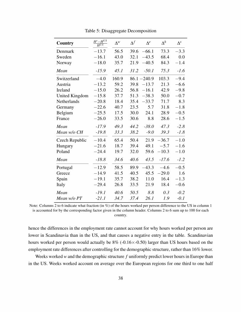
Table 5: Disaggregate Decomposition

Country Hc−HUS

HUS ∆w ∆ f ∆e ∆h ∆s

Denmark −13.7 56.5 39.6 −66.1 73.3 −3.3Sweden −16.1 43.0 32.1 −43.5 68.4 0.0Norway −18.0 35.7 21.9 −40.5 84.3 −1.4

Mean -15.9 45.1 31.2 -50.1 75.3 -1.6

Switzerland −4.0 160.9 86.1−240.9 103.3 −9.4Austria −13.2 59.2 39.8 −13.7 21.3 −6.6Ireland −15.0 26.2 56.8 −16.1 42.9 −9.8United Kingdom −15.8 37.7 51.3 −38.3 50.0 −0.7Netherlands −20.8 18.4 35.4 −33.7 71.7 8.3Germany −22.6 40.7 23.5 5.7 31.8 −1.8Belgium −25.5 17.5 30.0 24.1 28.9 −0.5France −26.0 33.5 30.6 8.8 28.6 −1.5

Mean -17.9 49.3 44.2 -38.0 47.3 -2.8Mean w/o CH -19.8 33.3 38.2 -9.0 39.3 -1.8

Czech Republic −10.4 65.4 50.4 21.9 −36.7 −1.0Hungary −21.6 18.7 39.4 49.1 −5.7 −1.6Poland −24.4 19.7 32.0 59.6 −10.3 −1.0

Mean -18.8 34.6 40.6 43.5 -17.6 -1.2

Portugal −12.9 58.5 89.9 −43.3 −4.6 −0.5Greece −14.9 41.5 40.5 45.5 −29.0 1.6Spain −19.1 35.7 38.2 11.0 16.4 −1.3Italy −29.4 26.8 33.5 21.9 18.4 −0.6

Mean -19.1 40.6 50.5 8.8 0.3 -0.2Mean w/o PT -21.1 34.7 37.4 26.1 1.9 -0.1

Note: Columns 2 to 6 indicate what fraction (in %) of the hours worked per person difference to the US in column 1is accounted for by the corresponding factor given in the column header. Columns 2 to 6 sum up to 100 for each

country.

hence the differences in the employment rate cannot account for why hours worked per person arelower in Scandinavia than in the US, and that causes a negative entry in the table. Scandinavianhours worked per person would actually be 8% (-0.16×-0.50) larger than US hours based on theemployment rate differences after controlling for the demographic structure, rather than 16% lower.

Weeks worked w and the demographic structure f uniformly predict lower hours in Europe thanin the US. Weeks worked account on average over the European regions for one third to one half

38

of the lower hours, and the demographic structure for another one third to one half. Differences inthe sectoral composition s play no significant role in explaining hours differences to the US in anyof the European countries. After controlling for the demographic and sectoral compositions in thisdecomposition exercise, we still observe marked patterns in the relative importance of employmentrates and weekly hours: in Scandinavia and Western Europe, weekly hours worked are the maindriver of lower hours per person compared to the US, explaining a share of 75 and 39 percent,respectively, with the employment rate going substantially in the opposite direction by 50 percentin Scandinavia, and slightly by 9 percent in Western Europe. Note that we exclude Switzerlandfrom the Western European average when discussing the results, because it features very highvalues in the decomposition table because of its small difference in hours worked per person to theUS of only -4%.24

While weekly hours universally point to lower hours in all Scandinavian and Western Europeancountries, though by varying degree, the employment rates do not universally indicate higher hours,with Belgium, France, and Germany being exceptions to this rule. In contrast to Scandinavia andWestern Europe, employment rates indicate lower hours worked per person in Eastern and SouthernEurope except Portugal, explaining on average 44 and 26 percent of the hours difference to the US,respectively. Portugal is the stark exception here, with employment rates indicating substantiallyhigher hours than in the US. Weekly hours go in the opposite direction in Eastern and SouthernEurope, indicating higher hours than in the US, with the exception of Spain and Italy. For Spainand Italy, weekly hours and employment rates are both roughly equally important in explainingthe hours gap to the US. In Portugal, lower hours are entirely driven by a lower number of workweeks and the demographic decomposition. Overall, the results in Table 5 make clear that thenegative cross-country correlation of the two components employment rates and weekly hours isnot primarily driven by differences in the demographic or sectoral compositions, but by some morefundamental factors that apply to all groups in the labor market.

By definition, the importance of work weeks is not affected by the demographic or sectoraldecomposition, as we impose the same number of work weeks for all subgroups within a country.We relax this assumption in Web Appendix Section W.6.3, where we allow for heterogeneity inweeks worked as described in Web Appendix Section W.2.5 by scaling the reported vacation weeksin the LFS data of each gender × age × education × sector group up by a common multiplicativefactor such that the average vacation weeks match the ones from external data sources. This pro-cedure (rather than assuming a common additive factor, or scaling up weeks worked rather than

24Remember that the hours differences to the US in this section are slightly different than the hours differences tothe US presented in Figure 7, because in this section we include only hours of individuals aged 15 to 64, not hours ofall working individuals aged 15 and above; see footnote 18.

39

vacation weeks) maximizes the degree of heterogeneity. Web Appendix Table W.18 shows theresults. While the results are almost unchanged for Scandinavia and Western Europe, allowing forheterogeneity in weeks worked by demographic group reduces the importance of the demographiccomposition in Eastern and Southern Europe by 9 and 14 percentage points, respectively, which isnearly completely offset by a corresponding increase in the importance of weeks worked.

Summarizing, there are three main findings from the disaggregate decomposition analysis.First, more vacation weeks alone account uniformly across Europe for between one third to onehalf of the hours difference to the US. Secondly, there exist large differences across Europe in therelative contribution of employment rates and weekly hours in explaining the hours difference tothe US even after controlling for differences in the demographic and sectoral composition. ForScandinavia and Western Europe, lower weekly hours worked explain three quarters and roughly40 percent, respectively, of the lower hours than in the US, with employment rates indicating higherhours than in the US. For Eastern and Southern Europe (excluding Portugal), by contrast, loweremployment rates explain roughly one half and one quarter, respectively, of the lower hours than inthe US, and weekly hours worked tend to be higher than in the US. Understanding the roots of thesedifferences constitutes an interesting new research agenda. Third, differences in the educationalcomposition constitute an important driving force of hours worked differences across countries:the different educational composition, with a higher share of low and medium educated people inEurope, accounts for one third to one half of the differences in hours worked per person, similarlyto weeks worked. Not taking the educational composition into account would overestimate theimportance of the employment rate in explaining lower hours in Eastern and Southern Europe, andwould underestimate the degree to which employment rates indicate higher hours in Scandinaviaand Western Europe than in the US

The results point to the importance of studying the educational composition as a driving forceof hours worked differences across countries. Which policies or other factors determine the differ-ent educational compositions across countries? For example, Restuccia and Vandenbroucke (2014)analyze the role of longevity and economic growth on the educational composition across countriesand over time. Note that some of these policies affecting educational choices could affect hoursworked directly at the same time. Guvenen et al. (2014), while not distinguishing between em-ployment and hours per employed, show that progressive taxation distorts the incentives to investin human capital, and that these tax differences can explain a sizable part of the differences in theEurope-US hours per person gap for men. Also, the results point to the importance of understand-ing why employment rates increase strongly with education within a country, but hours worked peremployed do not. Policies that affect the incentives to work differentially by education could e.g.

40

be welfare systems, or different degrees of flexibility in the labor markets for rich and poor, e.g.due to a minimum wage being binding for the poor. Moreover, the disutility of work could differin low- and high-education jobs. Yet, one would have to investigate if these factors influence theextensive margin more than the intensive one. In this regard, we want to mention the caveat thatcategorizing educational groups across countries in a consistent way is far from trivial, given thevastly different educational systems across countries.

6 Conclusion

In this paper, we document the construction of a new data set of aggregate hours worked startingfrom labor force surveys. This data set allows to analyze which fraction of the Europe-US hoursanalysis is driven by the different components of labor supply, as well as the role of the demo-graphic and sectoral composition. We rely on data from the US Current Population Survey, theEuropean Labor Force Survey, and the German Microcensus to construct hours worked measures.The main challenges for comparability of the several surveys at a given point in time across coun-tries, or for a given country over time, regard the sampling of reference weeks over the year and theunderreporting of vacation weeks. We show that we overcome both problems by obtaining hoursworked in a non-vacation week, i.e. a work week without a reduction in work time because of apublic holiday or annual leave, and requiring consistency of annual leave and public holidays in themicro data with the country-wide average. Information on the latter is collected from external datasources. While time trends in LFS and NIPA data are similar, we document substantial differencesin the level of the Europe-US hours gap in both types of data sources. In the LFS data, Europeanswork on average 19% fewer hours than Americans in the recent pre-crisis period 2005 to 2007,compared to only 7% in NIPA data. The likely reasons lie less in the slightly different coverageof the population, but more in the country-specific kinds of data sources and methodologies usedto construct NIPA hours, which might inhibit the international comparability. The differences be-tween LFS and NIPA data are large enough to matter for the measurement of labor productivityand the explanatory power of taxation for hours differences across countries.

In the main part of the paper, we decompose hours worked differences between Europe andthe US into weeks worked, employment rates, and weekly hours worked per employed in a non-vacation week, as well as the role of the demographic and sectoral composition in accounting forthese differences. Weeks worked and the demographic composition, driven by the educationalcomposition, both account for between one third and one half of the lower hours in Europe than inthe US. Weekly hours worked account for three quarters and roughly 40 percent of the lower hours

41

in Scandinavia and Western Europe, respectively, where employment rates contribute negativelyto explaining the hours gap to the US. By contrast, employment rates account for roughly one halfand one quarter, respectively, of the lower hours in Eastern Europe and Southern Europe withoutPortugal, with weekly hours worked mostly contributing negatively to the difference.

Our results indicate new avenues in the research agenda of the study of hours worked differ-ences across Europe and the US. First, they show that the higher number of vacation weeks inEurope is a significant driver of lower hours, and that longer vacation weeks are not associatedwith either higher employment rates or longer weekly hours worked. This might indicate thatthe number of work weeks is determined by other driving factors than those determining employ-ment rates and weekly hours worked, and raises the question whether they should be modeled as achoice variable for the individual. Secondly, we document a negative correlation between weeklyhours worked and employment rates across countries that is not entirely driven by differencesin the sectoral or educational composition. Modeling this negative correlation is not trivial, andinvestigating the sources is a promising research agenda. Third, the educational composition mat-ters significantly in accounting for cross-country differences in hours worked through its effect onemployment rates. Understanding why different education groups exhibit such different employ-ment rates (but not weekly hours worked), and different countries have such different educationalcompositions, will thus be a helpful step in explaining hours worked differences across countries.

ReferencesAlesina, A., E. Glaeser, and B. Sacerdote (2005). Work and Leisure in the United States and

Europe: Why So Different? NBER Macroeconomics Annual 20, 1–64.

Alonso-Ortiz, J. (2014). Social Security and Retirement Across the OECD. Journal of EconomicDynamics & Control 47, 300–316.

Bick, A., B. Bruggemann, and N. Fuchs-Schundeln (2016). A Note on the Europe-US Gap inHours Worked per Person: Data Revisions and Different Formulas. Working Paper.

Bick, A. and N. Fuchs-Schundeln (2016). Taxation and Labor Supply of Married Couples AcrossCountries: A Macroeconomic Analysis. Working Paper, Arizona State University and GoetheUniversity Frankfurt.

Bick, A., N. Fuchs-Schundeln, and D. Lagakos (2016). How Do Average Hours Worked Vary withDevelopment? Cross-Country Evidence and Implications. NBER Working Paper 21874.

Blundell, R., A. Bozio, and G. Laroque (2011). Labour supply and the extensive margin. AmericanEconomic Review Papers and Proceedings.

42

Blundell, R., A. Bozio, and G. Laroque (2013). Extensive and Intensive Margins of Labour Supply:Work and Working Hours in the US, the UK and France. Fiscal Studies 34, 1–29.

Bridgman, B., G. Duernecker, and B. Herrendorf (2016). Structural Transformation, Marketiza-tion, and Household Production Around the World. Working Paper.

Burda, M., D. Hammermesh, and P. Weil (2008). Working Hours and Job Sharing in the EU andUSA, Chapter The Distribution of Total Work in the EU and the US.

Burda, M., D. Hammermesh, and P. Weil (2013). Total Work and Gender: Facts and PossibleExplanations. Journal of Population Economics 26(1), 239–161.

Eldridge, L. P., M. E. Manser, and P. F. Otto (2004). Alternative measures of supervisory employeehours and productivity growth. Monthly Labor Review April, 9–28.

Erosa, A., L. Fuster, and G. Kambourov (2012). Labor Supply and Government Programs: ACross-Country Analysis. Journal of Monetary Economics 59, 84–107.

European Commission, International Monetary Fund, Organisation for Economic Co-operationand Development, United Nations, and World Bank (2009). System of National Accounts 2008.

Eurostat (2013). European System of Accounts ESA 2010.

Fang, L. and C. McDaniel (2016). Home Hours in the United States and Europe. B.E. Journal ofMacroeconomics: Advances Forthcoming.

Feenstra, R. C., R. Inklaar, and M. P. Timmer (2015). The Next Generation of the Penn WorldTable. American Economic Review 105(10), 31503182.

Fleck, S. E. (2009, May). International Comparisons of Hours Worked: An Assessment of Statis-tics. Monthly Labor Review 132(5), 3–31.

Frazis, H. and J. Stewart (2010). Why Do BLS Hours Series Tell Different Stories About Trendsin Hours Worked? BLS Working Paper 433.

Guvenen, F., B. Kuruscu, and S. Ozkan (2014). Taxation of Human Capital and Wage Inequality:A Cross-Country Analysis. Review of Economic Studies 81, 818–850.

Johnson, S., W. Larson, C. Papageorgiou, and A. Subramanian (2013). Is Newer Better? PennWorld Table Revisions and Their Impact on Growth Estimates. Journal of Monetary Eco-nomics 60(2), 255–274.

Kaplan, G. (2012). Inequality and the Life Cycle. Quantitative Economics 3, 471–525.

Koerner, T. and K. Marder-Puch (2015). Der Mikrozensus im Vergleich mit anderen Arbeitsmark-tstatistiken. WISTA – Wirtschaft und Statistik (4).

43

Krueger, D., F. Perri, L. Pistaferri, and G. L. Violante (2010). Cross-Sectional Facts for Macroe-conomists. Review of Economic Dynamics 13(1), 1–14.

McDaniel, C. (2011). Forces Shaping Hours Worked in the OECD, 1960-2004. American Eco-nomic Journal: Macroeconomics 3, 27–52.

McDaniel, C. (2012). Average Tax Rates on Consumption, Investment, Labor and Capital in theOECD 1950-2003. Working Paper.

Ohanian, L. and A. Raffo (2012). Aggregate Hours Worked in OECD Countries: New Measure-ment And Implications for Business Cycles. Journal of Monetary Economics 59(1), 40–56.

Ohanian, L., A. Raffo, and R. Rogerson (2008). Long-Term Changes in Labor Supply and Taxes:Evidence from OECD Countries, 1956-2004. Journal of Monetary Economics 55, 1353–1362.

Olovsson, C. (2009). Why Do Europeans Work So Little? International Economic Review 50(1),39–61.

Pilat, D. (2003). Measuring Hours Worked in OECD Countries. DSTI/EAS/IND/SWP(2003)10,OECD.

Pinkovskiy, M. and X. Sala-i-Martin (2016). Newer Need Not Be Better: Evaluating the PennWorld Tables and the World Development Indicators Using Nighttime Lights. NBER WorkingPaper 22216.

Prescott, E. C. (2004). Why Do Americans Work So Much More Than Europeans? FederalReserve Bank of Minneapolis Quarterly Review 28, 2–13.

Ragan, K. (2013). Taxes, Transfers and Time Use: Fiscal Policy in a Household Production Model.American Economic Journal: Macroeconomics 5(1), 168–192.

Ramey, V. A. (2012). The Impact of Hours Measures on the Trend and Cyclical Behavior of U.S.Labor Productivity. Working paper, University of California San Diego.

Restuccia, D. and G. Vandenbroucke (2014). Explaining Educational Attainment across Countriesand over Time. Review of Economic Dynamics 17(4), 824–841.

Rogerson, R. (2006). Understanding Differences in Hours Worked. Review of Economic Dynam-ics 9, 365–409.

Rogerson, R. (2008). Structural Transformation and the Deterioration of European Labor MarketOutcomes. Journal of Political Economy 116, 235–259.

Schnitzlein, D. D. (2011). Umfang und Folgen der Nichtinanspruchnahme von Urlaub in Deutsch-land. DIW Wochenbericht 51+52, 14–20.

Wallenius, J. (2014). Social Security and Cross-Country Differences in Hours: A General Equi-librium Analysis. Journal of Economic Dynamics and Control 37, 2466–2482.

44