SANDIA REPORT SAND96-2247 UC-122 Unlimited Release Printed September 1996

Hot Oiling Spreadsheet

RECEIVED

0 S T I MAR 0 5 1997

A. J. Mansure

Issued by Sandia National Laboratories, operated for the United States Department of Energy by Sandia Corporation. NOTICE: This report was prepared as an account of work sponsored by an agency of the United States Government. Neither the United States Govern- ment nor any agency thereof, nor any of their employees, nor any of their contractors, subcontractors, or their employees, makes any warranty, express or implied, or assumes any legal liability or responsibility for the accuracy, completeness, or usefulness of any information, apparatus, prod- uct, or process disclosed, or represents that its use would not infringe pri- vately owned rights. Reference herein to any specific commercial product, process, or service by trade name, trademark, manufacturer, or otherwise, does not necessarily constitute or imply its endorsement, recommendation, or favoring by the United States Government, any agency thereof or any of their contractors or subcontractors. The views and opinions expressed herein do not necessarily state or reflect those of the United States Govern- ment, any agency thereof or any of their contractors.

Printed in the United States of America. This report has been reproduced directly from the best available copy.

Available to DOE and DOE contractors from Office of Scientific and Technical Information PO Box 62 Oak Ridge, TN 37831

Prices available from (615) 576-8401, FTS 626-8401

Available to the public from National Technical Information Sebice US Department of Commerce 5285 Port Royal Rd Springfield, VA 22161

NTIS price codes Printed copy: A03 Microfiche copy: A01

DISCLAIMER

Portions of this document may be illegible in electronic image products. Images are produced from the best available original document.

SAND96-2247 Unlimited Release

Printed September 1966

Distribution Category UC-122

Hot Oiling Spreadsheet AJ. Mansure

Geothermal Research Department Sandia National Laboratories

Albuquerque, NM 87185

Abstract

One of the most common oil-field treatments is hot oiling to remove p a r e fiom wells. Even though the practice is common, the thermal effectiveness of the process is not commonly understood. In order for producers to easily understand the thermodynamics of hot oiling, a simple tool is needed for estimating downhole temperatures. Such a tool has been developed that was distributed as a compiled, public-domain-sohare spreadsheet. That spreadsheet has evolved into a interactive fiom on the World Wide Web (http://www.sandia.gov/apt/) and has been adapted into a Windowsm program by Petrolite, St. Louis MO. The development of such a tools was facilitated by expressing downhole temperatures in terms of analytic formulas. Considerable algebraic work is required to develop such formulas. Also, the data describing hot oiling is customarily a mixture of practical units that must be converted to a consistent set of units. To facilitate the algebraic manipulations and to assure unit conversions are correct, during development parallel calculations were made using the spreadsheet and a symbolic mathematics program. Derivation of the formulas considered falliig film flow in the annulus and started from the transient differential equationsso that the effects of the heat capacity of the tubing and casing could be included. While this approach to developing a s o h a r e product does not have the power and sophistication of a finite element or difference code, it produces a user fiiendly product that implements the equations solved with a minimum potential for bugs. This allows emphasis in development of the product to be placed on the physics.

ACKNOWLEDGMENTS

This work performed at Sandia National Laboratories supported by the U.S. Department of Energy (DOE) under contract DE-ACO4-76DPOO789. The par& control study at Sandia, which the development of the Hot Oiling Spreadsheet was a part, was sponsored by the Natural Gas and Oil Technology Partnership, a DOE program of cooperative work between the national labs and industry. The industrial partner that worked with Sandia on the par& control work was Petrolite of St. Louis, Mo. The contributions of Ken Barker, the principal investigator at Petrolite, are gratefully acknowledged for his identification of the physical processes that control the effectiveness of hot oiling jobs.

INTRODUCTION

While hot oiling is a co&on oil field practice there is little appreciation of the thermal effectiveness of hot oiling. To change this situation a spreadsheet has been developed to estimate downhole temperatures during hot oiling. The spreadsheet was developed as an educational tool and makes a number of simplifying assumptions. If accurate predictions of downhole temperature are required, a more sophisticated code should be used.' The challenge was to develop user- fiiendly, interactive, public-domain s o h a r e that will run on any PC. However, it is also important that the code be as physically accurate as possible. While there are a number of simple analytic models that have been used for predicting downhole temperatures during injection, drilling, or they make assumptions that are not valid for hot oiling. There are of course fkite element or finite difference codes that could be adapted for the calculations, but this approach was not deemed to meet the user-fiiendly, interactive, and public-domain goals. A significant challenge in the development of this tool was insuring that the equations and unit conversions were correctly input into the spreadsheet. Spreadsheets while being user friendly to use are dficult to debug. Thus, as part of the verification of the spreadsheet, the equations were solved, including units, with a symbolic logic program (Mathematica, http://www.wri.com/) and the results were shown to be the same as the spreadsheet to three significant figures.

Initially the tool developed to satis@ these requirements was a DOS based complied spreadsheet that executes as a stand-alone program (Figure I). When World Wide Web technology became available, the spreadsheet was converted to a interactive form that can be accessed over the INTERNET at http://www.sandia.gov/apt/ (Figure 2). The form launches a Visual BasicTM program that does the calculations based on the user's inputs and creates the hypertext document that is served back to the user. Petrolite of St. Louis MO has developed a WmdowsTM program based on the original DOS spreadsheet (Figure 3). AU three of these tools allow the user to interactively input data and receive the results of the calculations either as a table or graph (Figure 4.).

The intent of this report is to document the assumptions, empirical formulas used, and other information about the spreadsheet. As such it is a collection of separate topics written to document various aspects of the spreadsheet. While it lacks completeness or flow from one topic to the next, its value to those who are already using the spreadsheet makes it important to publish it as rather than let the work go undocumented.

In a "hot oiling" job oil or water is injected down the annulus of an oil well in an attempt to melt paraffin that has deposited in the tubing. The heat capacity of the fluid injected is smaller than the heat capacity of the casing and tubing and there is heat loss to the surrounding rock. Thus the oil injected cools rapidly. The effectiveness of hot oivwatering depends on the depth to

1

which the tubing is raised above the melting point of the par&. Because of this rapid cooling of the injected fluid, the assumption of quasi-static equilibium assumed in previous work needed to be investigated, thus the development of the spreadsheet started with the transient differential equations.

Sometimes Joule-Thomson cooling during production can cool the production interval enough to drop the temperature below the cloud point and cause par@ to precipitate at the production interval. Being able to calculate if this happens can be important in analyzing paraffin problems and thus such calculations have been included in the spreadsheet.

The development of a practical approach to estimating hot oiling temperatures has involved a number of various investigations which constitute the sections of this document: 0

0

0

0

0

SPREADSHEET EWIRICAL FORMULAS: establishing empirical formulas for fluid properties, falling film flow, heat transfer coefficients, and heat loss to the earth, QUASI-STATIC APPROXIMATION: investigation of quasi-static equilibrium assumption for case of no flow in the tubing, DERIVATION COUNTER-FLOW EQUATIONS: derivation of counter flow equations assuming quasi-static equilibrium, but accounting for the depth the thermal transient penetrates the well fiom the surface, JOULE-THOMSON COOLING: development of approach for calculating the temperature of gas flow up the annulus during production. VERIFICATION OF HOT OILING SPREADSHEET: verification of hot oiling and hot watering calculations with field data.

2

SPREADSHEET EMPIRICAL FORMULAS

Average Fluid Temperature

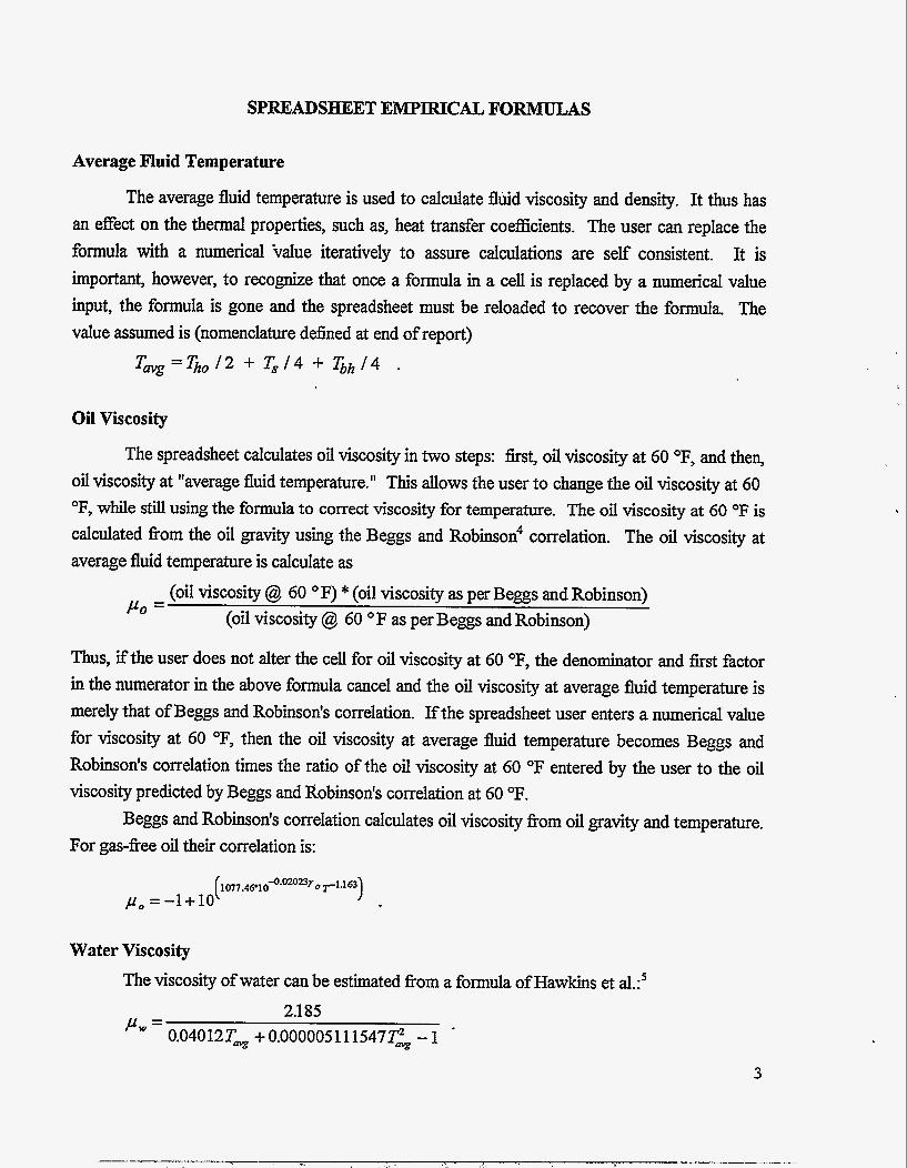
The average fluid temperature is used to calculate fliid viscosity and density. It thus has an effect on the thermal properties, such as, heat transfer coefficients. The user can replace the formula with a numerical 'value iteratively to assure calculations are self consistent. It is important, however, to recognize that once a formula in a cell is replaced by a numerical value input, the formula is gone and the spreadsheet must be reloaded to recover the formula. The value assumed is (nomenclature defined at end of report)

Twg=G0 I 2 + G I 4 + &h/4 .

Oil Viscosity

The spreadsheet calculates oil viscosity in two steps: first, oil viscosity at 60 O F , and then, oil viscosity at "average fluid temperature." This allows the user to change the oil viscosity at 60 OF, while still using the formula to correct viscosity for temperature. The oil viscosity at 60 OF is calculated fiom the oil gravity using the Beggs and Robinson4 correlation. The oil viscosity at average fluid temperature is calculate as

- (oil viscosity @ 60 OF) * (oil viscosity as per Beggs and Robinson) (oil viscosity @ 60 O F as per Beggs and Robinson) Po -

Thus, ifthe user does not alter the cell for oil viscosity at 60 OF, the denominator and first factor in the numerator in the above formula cancel and the oil viscosity at average fluid temperature is merely that of Beggs and Robinson's correlation. If the spreadsheet user enters a numerical value for viscosity at 60 OF, then the oil viscosity at average fluid temperature becomes Beggs and Robinson's correlation times the ratio of the oil viscosity at 60 OF entered by the user to the oil viscosity predicted by Beggs and Robinson's correlation at 60 O F .

Beggs and Robinson's correlation calculates oil viscosity fiom oil gravity and temperature. For gas-free oil their correlation is:

Water Viscosity The viscosity of water can be estimated fiom a formula of Hawkins et al.?

P w - O.O4012T, + 0.00000511 1547T; - 1 - 2.1 85

3

Oil Density

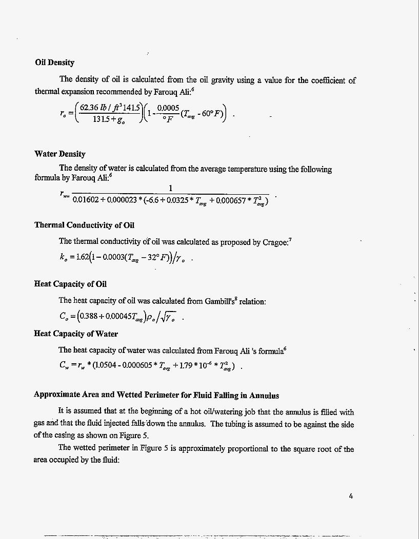
The density of oil is calculated fiom the oil gravity using a value for the coefficient of thermal expansion recommended by Farouq Ak6

ro = (62.36 Zl~/$~141.5)( 1 --(T, 0.0005 -6O'F)) . 13 1.5 +go " F

Water Density

formula by Farouq Ali! The density of water is calculated fiom the average temperature using the following

1 rw 0.01602 + 0.000023 * (-6.6 + 0.0325 * T, + 0.000657 * T') -

Thermal Conductivity of Oil

The thermal conductivity of oil was calculated as proposed by Cragoe:'

k, = 1.62(1- O.O003(T, - 32'F))/yO .

Heat Capacity of Oil

The heat capacity of oil was calculated from GambU'ss relation:

Co = (0.388 + 0.00045T,)pO/& .

Heat Capacity of Water

The heat capacity of water was calculated from Farouq Ali Is formula6

Cw =rw * (1.0504 - 0.000605 * Tw + 1.79 * loa * T&) .

Approximate Area and Wetted Perimeter for Fluid Falling in Annulus

It is assumed that at the beginning of a hot oil/watering job that the annulus is filled with gas and that the fluid injected falls'down the annulus. The tubing is assumed to be against the side of the casing as shown on Figure 5.

The wetted perimeter in Figure 5 is approximately proportional to the square root of the area occupied by the fluid:

4

Figure 5 : Position of tubing within casing showing area (shaded region) occupied by fluid.

For channel flow the Chky formulag relates velocity, fiiction factor, wetted perimeter, and area:

v . / ( 7 ) = A 1 / P .

The Reynolds number and fiiction factor can be written in terms of the area as

Re = 4P!21 and f = 0.184 Re-.02 = 0.184 P P I K

These equations can be combined and solved for the area to get

Annular Heat Transfer CoeEcient

The annular heat transfer coefficient can be calculated using the following formulas:lO Dh = 4 A, / P Re = Dh (V)P/P (v) = Qi /A1 P, = C p / k Nu, = 0.0296Re0.8 Pr” h = Nu, k /Dh

5

Heat Loss to the Earth

Ramey2 showed how the heat lost to the earth can be approximated by a parameter

where C is the heat capacity of the fluid in the annulus, k is the conductivity of the surrounding earth, and U is the overall heat transfer coefficient as discussed by Willhite." For hot odfwatering jobs, U is typically large enough thatfp) is closer to a constant temperature than constant flw boundary condition. The analytic solution for this boundary condition is12

which can be approximated as (y<5): 1

(v)" + 0.35 - 0 . 0 6 7 ( y / ~ ) ~ f O =

For hot oilfwatering jobs the time of heat transfer is short enough that the difference in thermal conductivity of the "cement" surroundmg casing and the earth can be important. This can be corrected for using the following empirical equation:

where kc is the conductivity of the cement, ke is the conductivity of the earth, and

m = (1.976 - 1.69RW f Rh)Ln[Rh f R,] .

Joule-Thomson Cooling

For oil and water free gas expanding fkom a high formation pressure to a low flow-line pressure the Joule-Thomson cooling can be approximated as

= (O.O48OF f p.i)AP .

6

QUASI-STATIC APPROXIMATION

Including the effects of the heat capacity of the fluid in the annulus results in the following time dependent generalization of Ramey's' differential equation:

62' 62' sign T-T , -+&-+-+-- - 0 a J * C A[t]

where Q is positive for flow down the well and negative for flow up the well, sign = 0 for liquid flow in the well, sign = -1 for gas flow down the well, sign = +1 for gas flow up the well, and

E = A, /Q, T,=a.z+T,

T = a - z + T , +F,[f]+B[z,t] Let

where B[z,t] is a finction that goes to zero far fiom where fluid enters the well and F,[t] is a fhction governing the shift in temperature of a flowing well with no fluid injection, thus

Fo[O] = 0

L o =Tho - The equation can be solved by Laplace transform techniques to give

Unfortunately these integrals can not be solved in closed form. In the quasi-static approximation, these integrals are solved assuming that Act] is a constant independent of time and then the appropriate time dependent value ofA[ t ] is plugged into the approximate solutions. For constant A[t] or the quasi-static approximation, the above expressions become

F,4s [ t ] 3 -(E + e) A"[ 1 - and E C d

for z < tk and zero for z > tk. The depth t/E is the depth the transient solution has propagated 7

down the well. Note: if the quasi-static approximation is made to 'the differential equation (Ramey's formulation) the temperature disturbance continues to infinity. Thus, one important addition to Ramey's solution is to cut it off at t /~ .

integrated using the following approximation for A b ] : To test the adequacy of this approximation the integral solution was numerically

A*pprx. [rl= 332(Ln[874y + x ] ) ~ .

In order to do the numerical integration it is necessary to assume a value for E. The value assumed was 0.0004. The conclusion is not significantly dependent upon the E assumed as was demonstrated by varying the value of E. Figure 6 compares numerically integrated solution with the quasi-static approximation. The figure shows discrepancies, but FO[t] appears quite good for. small times -- hot owwatering jobs typically have t < 1. The plot of the quasi-static B[z,t] shows a square shoulder at the cutoff depth, where as, the numerically integrated solution is rounded. Fortunately, the depth the spreadsheet needs to be accurate is back up the well above the "thermal fiont" (-500 R) where the increase in temperature is high enough to be above the wax melting point. At these depths the error in the quasi-static solution is only a few percent.

1

0.8

Fo[t] 0.4

0.2

2 4 6 8 10

t 1000 2000 3000 4000

Depth Figure 6: Comparison of quasi-static solution and numerically integrated solution.

The above equations apply when the annulus has fluid in it. At the beginning of a hot owwatering job the annulus is typically empty. Clearly below the depth the fluid has fallen or reached, there will be no change in temperature. The depth t/s is the depth to which the thermal fiont has advanced down the well. This depth will be less than the depth the fluid has fallen.

The case considered here is for a single flow stream, down the annulus only. When there is flow down the annulus and up the tubing the problem becomes more complex and the time dependent equations can not be solved in integral form. However, the evaluation of the quasi- static solution above indicates that it can be used, provided that the transient solution is cutoff at the right depth.

8

DERIVATION OF COUNTER-FLOW EQUATIONS

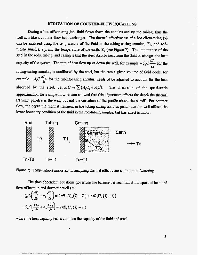
During a hot oivwatering job, fluid flows down the annulus and up the tubing; thus the well acts like a counter-flow heat exchanger. The thermal effectiveness of a hot oivwatering job can be analyzed using the temperature of the fluid in the tubing-casing annulus, Ti, and rod- tubing annulus, To, and the temperature of the earth, Te (see Figure 7). The importance of the steel in the rods, tubing, and casing is that the steel absorbs heat from the fluid or changes the heat

capacity of the system. The rate of heat ffow up or down the well, for example -QIC- for the

tubing-casing annulus, is unaffected by the steel, but the rate a given volume of fluid cools, for 32

example -A,C- dT, for the tubmg-casing annulus, needs of be adjusted to account for the heat dt

absorbed by the steel, i.e., A,C + c(A,C, + A&). The discussion of the quasi-static

approximation for a single-ff ow stream showed that this adjustment affects the depth the thermal transient penetrates the well, but not the curvature of the profile above the cutoff. For counter ffow, the depth the thermal transient in the tubmg-casing annulus penetrates the well affects the lower boundary condition of the fluid in the rod-tubing annulus, but this effect is minor.

Rod Tubing

TO

Tr-TO Tt-TI

TI

Casing

Earth - Te

TC-TI

Figure 7: Temperatures important in analyzing thermal effectiveness of a hot oillwatering.

The time dependent equations governing the balance between radial transport of heat and flow of heat up and down the well are

where the heat capacity terns combine the capacity of the fluid and steel

9

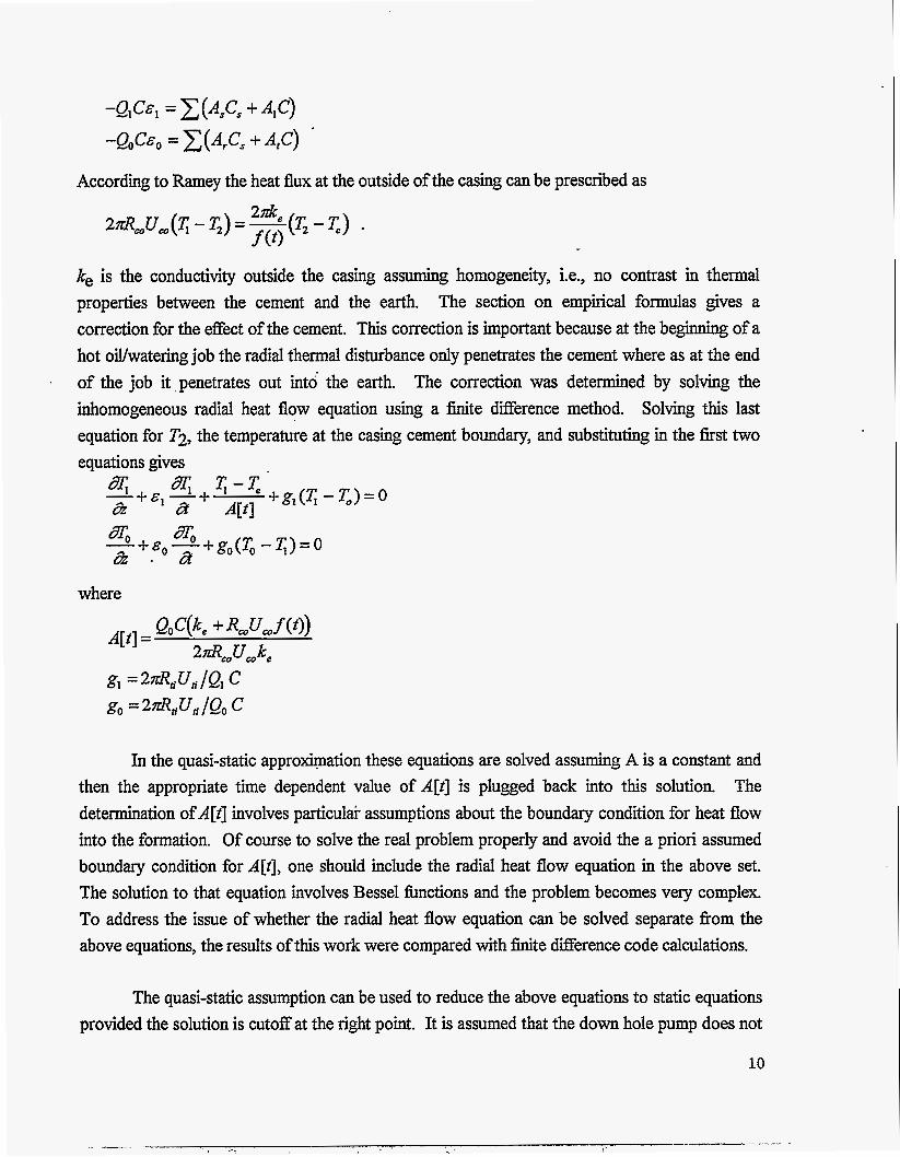
According to Ramey the heat flux at the outside of the casing can be prescribed as

ke is the conductivity outside the casing assuming homogeneity, i.e., no contrast in thermal properties between the cement and the earth. The section on empirical formulas gives a correction for the effect of the cement. This correction is important because at the beginning of a hot oivwatering job the radial thermal disturbance only penetrates the cement where as at the end of the job it ,penetrates out into the earth. The correction was determined by solving the inhomogeneous radial heat flow equation using a finite difference method. Solving this last equation for 7'2, the temperature at the casing cement boundary, and substituting in the first two equations gives

where

In the quasi-static approMation these equations are solved assuming A is a constant and then the appropriate time dependent value of A[t] is plugged back into this solution. The determination ofA[t] involves particulai assumptions about the boundary condition for heat flow into the formation. Of course to solve the real problem properly and avoid the a priori assumed boundary condition for Art], one should include the radial heat flow equation in the above set. The solution to that equation involves Bessel finctions and the problem becomes very complex. To address the issue of whether the radial heat flow equation can be solved separate fiom the above equations, the results of this work were compared with finite difference code calculations.

The quasi-static assumption can be used to reduce the above equations to static equations provided the solution is cutoff at the right point. It is assumed that the down hole pump does not

10

introduce any thermal transients arid that below the heat-fiont propagating down the well fiom the surface, temperatures are in equilibrium with the earth, i.e. for z*q > t that Ti = To = T,. With these assumptions the differential equations reduce to

subject to the boundary conditions T1IFo = Tho and T o l d E = Te There is thus a moving boundary condition for the ffuid in the tubing. The solution to the above set of equations is conceptually straight forward but algebraically complex. They are most readily solved by assuming finctions of the right algebraic form and usiig a symbolic mathematics program to solve the resulting equations for the coefficients and boundary conditions. Below the cutoff point Ti =

T2 = T,. Above the cutoff point t/E

I ; = T, + c, - T, = T, +e,c,

+ c2 - e+' - ~ [ t ] . a(1 + g, /go) + e 2 2 c :e+' - ~ [ t l - a ( l + g , / g o ) - a / g o

where

11

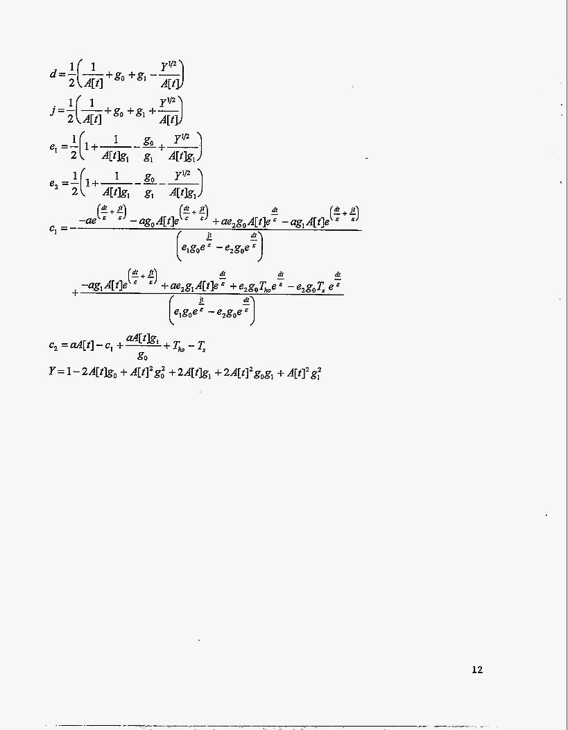
dt - dt - dt (; + ;) - -a& 4 1 e + ae,g, A[@ E + e,goT,e - e,goT, e E

f it dt \ +

+T,-T, 4N& c, = aA[t] - c1 + go

12

JOULE-THOMSON COOLING

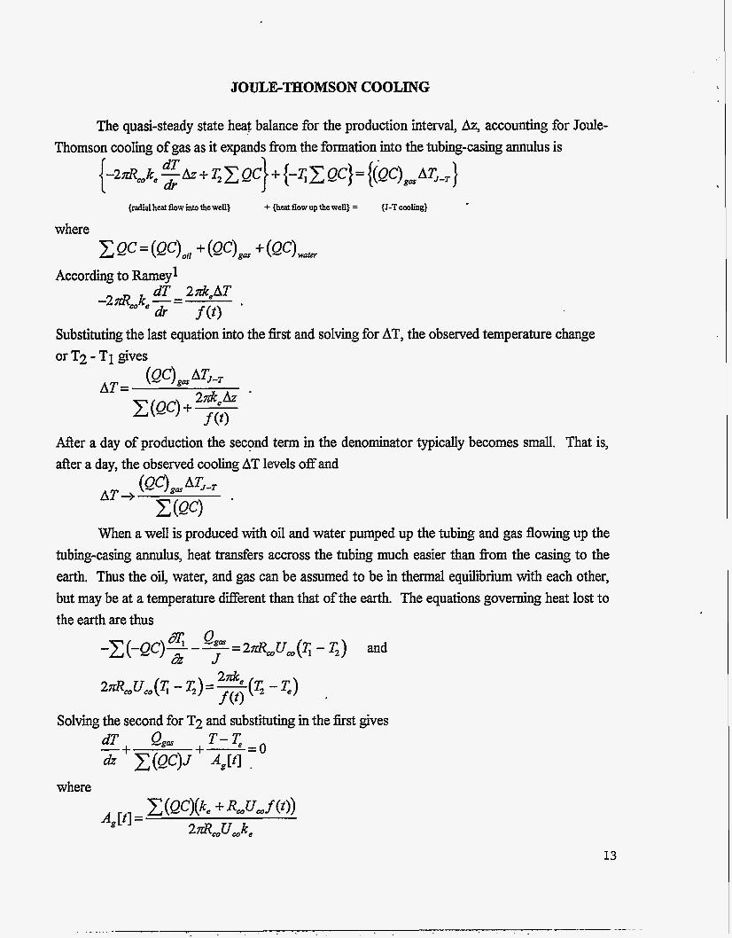
The quasi-steady state heat balance for the production interval, ~4 accounting for Joule- Thomson cooling of gas as it expands from the formation into the tubing-casing annulus is

{-27rRmke $Az+ T,c QC}+ { -qzQC)= {(QC) ga AT,-,}

{radial heat flow into the well) + {heat flow up the well) =

where {J-T COobg}

Qc = (QC)oil + (W), + (QC) water

According to Rameyl dT 2deAT -278 k - =

f ( t ) *

Substituting the last equation into the first and solving for AT, the observed temperature change or T2 - Ti gives

After a day of production the second term in the denominator typically becomes small. That is, after a day, the observed cooling AT levels off and

(Qc) AT,-, AT 3 C ( Q C )

When a well is produced with oil and water pwnped up the tubing and gas flowing up the tubing-casing annulus, heat transfers accross the tubing much easier than from the casing to the earth. Thus the oil, water, and gas can be assumed to be in thermal equilibrium with each other, but may be at a temperature different than that of the earth. The equations governing heat lost to the earth are thus

Solving the second for T2 and substituting in the first gives -

T - T , +-- - 0 dT Qga -+ * C ( Q C ) J AgP1 . where

13

For production with Joule-Thomson cooling at the formation the boundary condition is

The solution to the differential equation with this boundary condition is

- q z = D - T I z = D - ' T - T *

14

VERIFICATION OF HOT OILING SPREADSHEET

While the physics included in the calculations done by the Hot Oiling Spreadsheet is basic, there is always questions as to whether a set of calculations includes the right physics and is the physics coded correctly. To address these questions, a series of field tests were done in attempt to veritj, the Hot Oiling Spreadsheet. At the time these field tests were started, there was no practical way to measure downhole temperatures during hot oiling. Hence, a parallel effort to develop downhole rod coupling temperature monitors was initiated. The development of these is documented as part of the Applied Production Technology home page on the INTERNET (http://www.sandia.gov/apt/). These were only available for limited use during the verification of the spreadsheet. Unfortunately, no verification has been done of the Joule-Thomson cooling calculations.

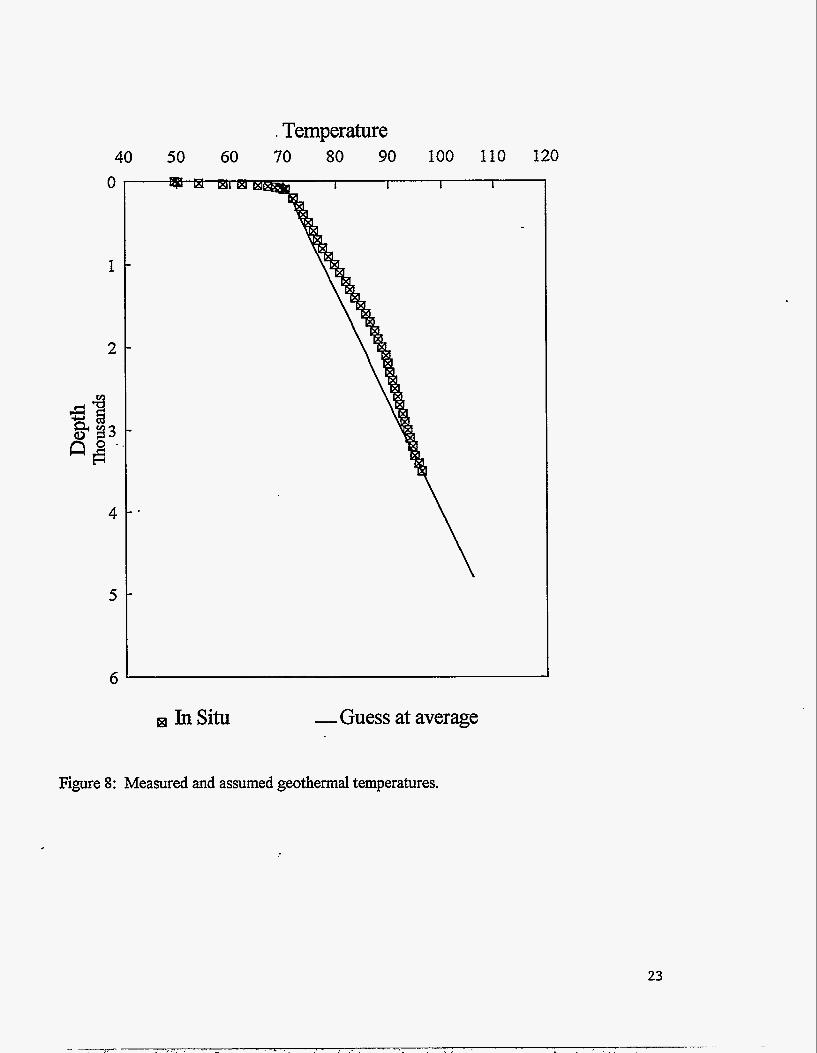
Field tests of the heat transfer that occurs during hot oiling or hot watering were made by setting a bridge plug between the perforations and bottom of the tubing so that fluid could be circulated without entering the formation. The temperature was logged before the experiment to determine the geothermal temperature. Temperature was recorded inside the tubing at 300 feet while hot fluid was circulated and immediately after circulation was stopped the temperature in the tubing was logged. Before the test, the well was filled with oil, circulated, and allowed to equilibrate. At the end of the first day the oil was displaced with water. The next day hot water was circulated. Thus, the thermal disturbance fiom circulating the oil had a day to dissipate before hot water was circulated. Radial heat flow calculations indicate that the temperature increase due to the hot oil should be down to - 5% the next day.

Figure 8 shows the geothermal temperature measured before the work began (squares with an x). It was winter, hence the cooling of the first 100 feet near the surface. Note, however, there also is a change in gradient near 2000 feet. Thus assuming a constant geothermal gradient introduces some error in the calculations. The assumed geothermal temperatures are shown by the straight line on the figure.

Figure 9 compares the temperature logged immediately after circulating oil with that predicted by the spreadsheet. The curves marked Tubing and Annulus were calculated by the spreadsheet. The curve marked 1 BPM is that measured. The calculations were done using Version 2 of the spreadsheet with one change: the equations were modified so that the annulus was full of fluid at the beginning of the job. The figure shows that the temperature measured inside the tubing at the end of the job is close to what the spreadsheet predicts for the tubing temperature, but is systematically less. In making this calculation, none of the typical input parameters (thermal properties of the earth, etc.) were changed from the defaults in the spreadsheet. While the discrepancy is no more than expected due to uncertainties in the typical

15

input parameters, the nature of the discrepancy suggests that it may be due to ignoring the Surface casing. Overall, the maximum discrepancy, at the end of this long job, is only about 10 OF, which is within the uncertainty due to the typical input parameters or within the accuracy the spreadsheet was designed to give.

Figure 10 shows temperature as a fkction of time 300 feet down the tubmg taken with a downhole rod coupling temperature monitor. The agreement between the spreadsheet and measured data is quite good. As before, the typical input parameters were not changed fiom the defaults in the spreadsheet. The calculations shown do not consider the surface casing which is set at 341 feet or below the depth of the measurement. Including surface casing improves agreement. The figure assumes that the process began when the first measurement was taken. However, since heat had already reached 300 feet the hot oiling truck must have been started some time earlier. Accounting for this will shift the measured data to the right improving the agreement.

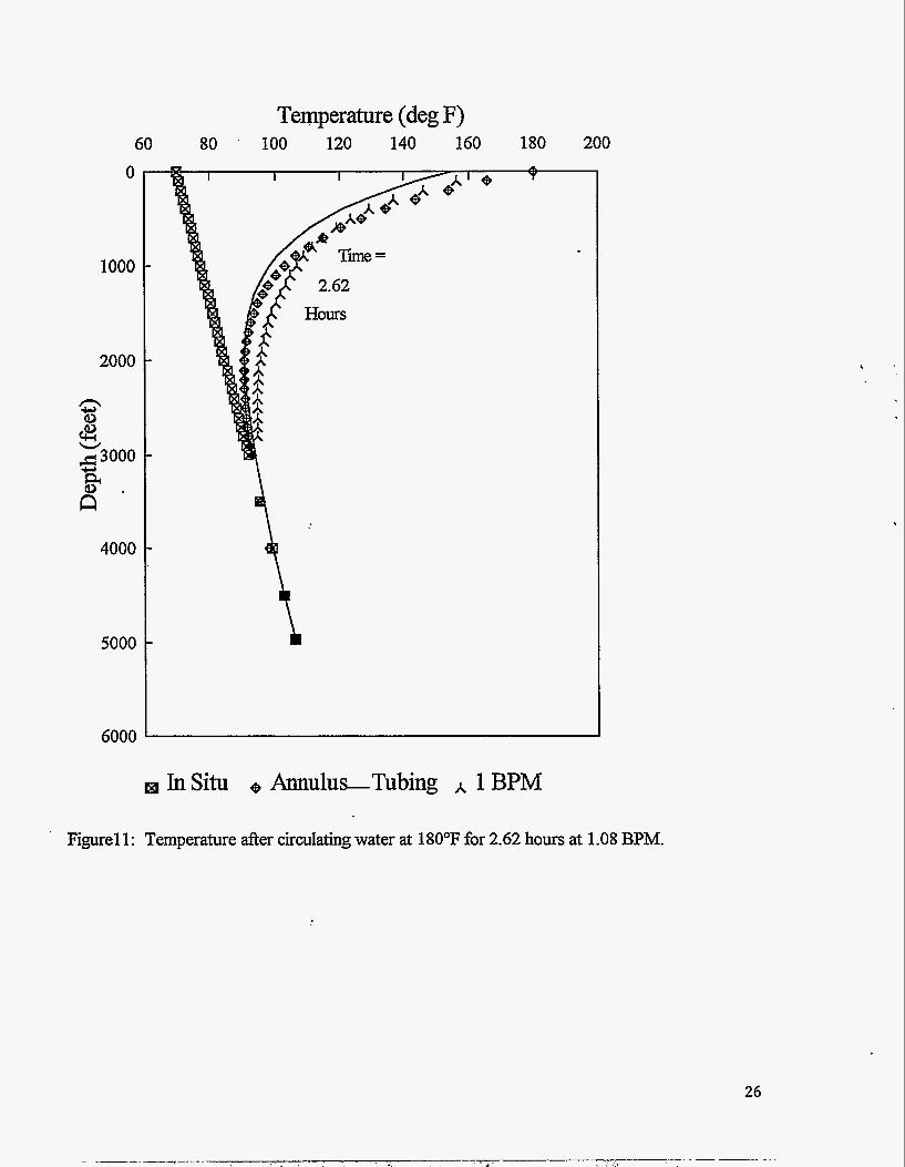
Figure 11 compares the temperature logged immediately after circulating water with that predicted by the spreadsheet. One additional change in the spreadsheet was made for these calculations: the fluid in the tubing was assumed to be water rather than oil. At first glance the agreement does not appear to be as good as for oil circulation; however, the Surface temperature is raised 5°F to account for the heat left over fiom the day before, the agreement for hot watering is just as good as for hot oiling.

In conclusion, the spreadsheet has been shown to be a reasonable tool for estimating hot oiling and hot watering downhole temperatures.

CONCLUSIONS

The goal in developing the Hot Oiling Spreadsheet was to provide a public-domain, user- friendly program for evaluating the effectiveness of hot oiling jobs. The success in meeting such a goal is determined by how much the program is used by the customer, the oil patch. Sandia has received over 200 requests for copies of the spreadsheet. Further, a number of companies have written indicating they make their own copies and distribute them as part of in-house training. Recognition of the value of the spreadsheet as a educational tool resulted in requests fiom industry to place the hot oiling spreadsheet on the INTERNET. Petrolite, St. Louis MO, has used the physics documented here to develop a WindowsTM version of the spreadsheet for use in their par& control schools. Short articles on the Sandia’s work on paraffin control including the spreadsheet have appeared in the Oil & Gas Journal, World Oil, and The American Oil & Gas Reporter. Thus there has been a high recognition of the value of the spreadsheet by the customer and the goals set in developing the spreadsheet have been met. This recognition of the value of the spreadsheet has been the impetus to document the physics of the spreadsheet in this report.

17

NOMENCIATURE

a Geothermal gradient, OF/A, A[t] A&] A function governing heat transfer to the earth during production, Ao A1 A, Ar C Cs Dh Hydraulic diameter, A, f g Acceleration of gravity, Wsec2, J k Fluid thermal conductivity, Btu/A-hr-OF, h Heat transfer Coefficient, Btu/ft2-hrY

k, Earth thermal conducti~ty, Btulft-hr-OF, Nud Nusselt number, P Wetted Perimeter, &, Pr Prandlt number, Qg Gas production rate, Ib3hh,. Qo Q1 %i Casing inside radius, A, Q0 Casing outside radius, ft, Re Reynolds number, Rh Radius of hole, ft, Rti Tubing inside radius, ft, Rto Tubing outside radius, ft, r radial distance, A, t Time, hr, T Temperature, OF, Tavg Average fluid temperature, OF, Te Temperature of the Earth, OF, Tg Gas temperature during production, OF, Tho Temperature of injected fluid, OF, Tr Mean rod temperature, OF, Ts Mean surface temperature, OF, Tt Mean tubing temperature, OF, Tc Mean casing temperature, OF, Tbh Bottomhole temperature, OF, T i

A function governing heat transfer to the earth,

Area of fluid in the rod-tubing annulus, A2, Area of fluid in the tubing-casing annulus, A2, Area of steel in the tubing and casing, ft2, Area of fluid in the rods, ft2, Heat capacity of fluid, Btu/lb-"F, Heat capacity of steel, Btu/lb-OF,

Friction factor (Moody or Darcy),

Mechanical equivalent of heat, 777.97 Ib-fl/Btu,

Cement thermal conductivity, Btu/ft-hr-OF,

Rod-tubing annulus volume flow rate, Ib/min, Tubing-casing annulus volume flow rate, Ib/min,

Temperature of the oil in the annulus between the casing and the tubing, O F , 18

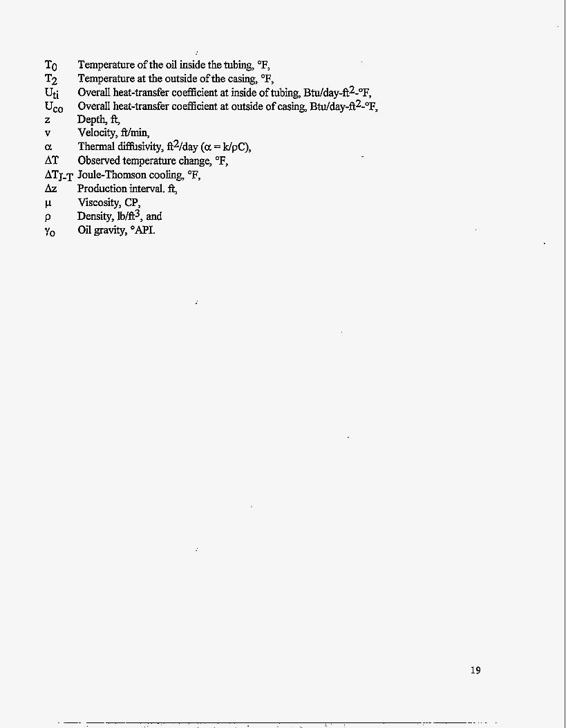
To T2 Uti Uco z Depth,fiy v Velocityy Wmin, a AT Observed temperature change, OF, AT J-T Joule-Thomson cooling, OF, Az Production interval. fi, p Viscosityy CP, p Densityy lb/ft3, and 'yo Oil gravityy O A P I .

Temperature of the oil inside the tubing, OF, Temperature at the outside of the casingy OF, Overall heat-transfer coefficient at inside of tubing, Btu/day-fi2-OFY Overall heat-transfer coefficient at outside of casing, Btu/day-fi2-°Fy

Thermal diffusivityy fi2/day (a = k/pC),

19

REFERENCES

1.

2. 3.

4.

5.

6.

7. 8. 9. 10.

11.

12.

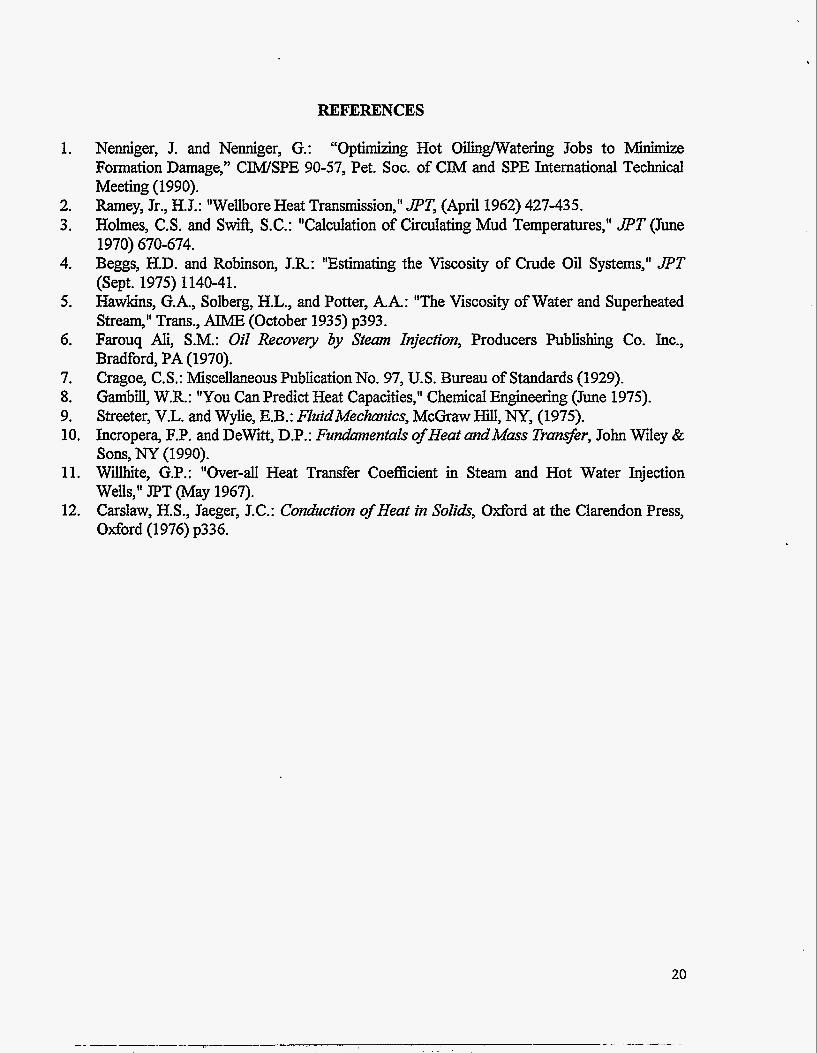
Nenniger, J. and Nenniger, G.: "Optimizing Hot Oiling/watering Jobs to Minimize Formation Damageyy7 CMSPE 90-57, Pet. SOC. of CIM and SPE International Technical Meeting (1990). Ramey, Jr., H.J.: "Wellbore Heat Transmission," PT, (April 1962) 427-435. Holmes, C.S. and Swift, S.C.: "Calculation of Circulating Mud Temperatures," JPT (June

Beggs, H.D. and Robinson, J.R: "Estimating the Viscosity of Crude Oil Systems," P T (Sept. 1975) 1140-41. Hawkins, G.A, Solberg, H.L., and Potter, AA: "The Viscosity of Water and Superheated Stream," Trans., AlME (October 1935) p393. Farouq Ali, S.M.: Oil Recovery by Steam Injection, Producers Publishing Co. Inc., Bradford, PA (1970). Cragoe, C.S.: Miscellaneous Publication No. 97, U.S. Bureau of Standards (1929). Gambill, W.R.: "You Can Predict Heat Capacities," Chemical Engineering (June 1975). Streeter, V.L. and Wylie, E.B.: FIuidMechics, McGraw Hill, NY, (1975). Incropera, F.P. and DeWitt, D.P.: Fundamentals of Heat andMass E w e r , John Wiley & Sons, NY (1990). Willhite, G.P.: "Over-all Heat Transfer Coefficient in Steam and Hot Water Injection Wells," JPT (May 1967). Carslaw, H.S., Jaeger, J.C.: Conduction of Heat in Solids, oxford at the Clarendon Press, Oxford (1976) p336.

1970) 670-674.

Figure 1: DOS based complied spreadsheet.

21 Figure 2: Interactive form on the INTERNET.

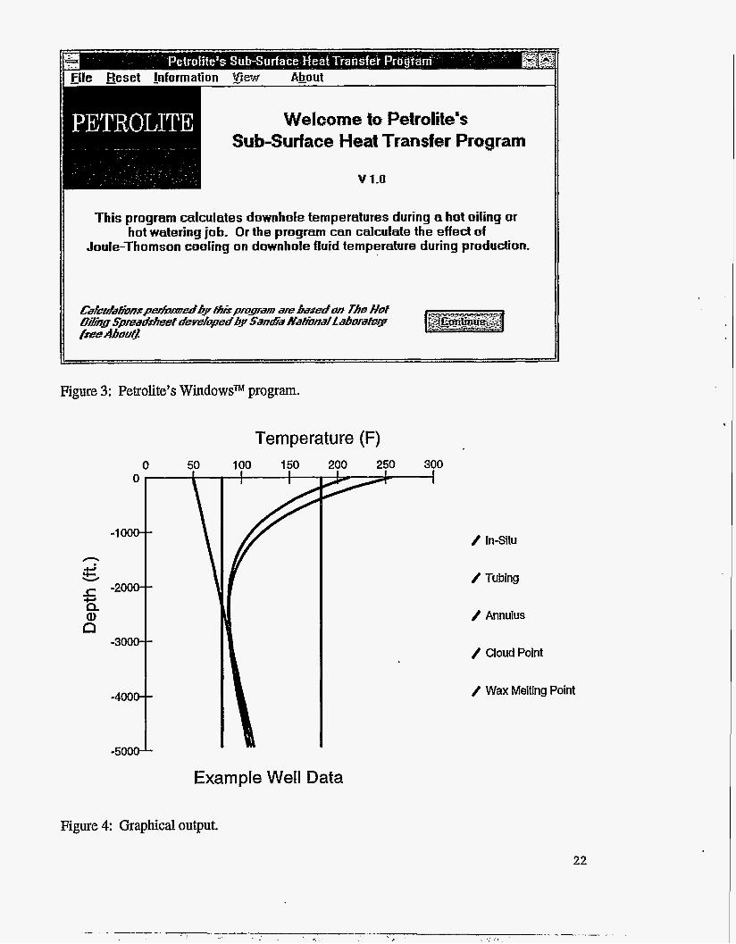
PETROLITE Welcome to Fetrdite% ~ Sub-Surface Heat Transfer Program

v 1.0

This program calculates downhole temperatures during a hot oiling or hot watering job. Or the program can calculate the effed of

Joule-Thomson cooling on downhole fluid temperature during production.

Figure 3: Petrolite’s WindowsTM program.

Temperature (F)

c ?= c

0 In-Situ

0 Tubing

0 Annulus

/ Cloud Point

0 Wax Melting Point

Example Well Data

Figure 4 Graphical output.

22

. Temperature 40 50 60 70 80 90 100 110 120

69 InSitu - Guess at average

Figure 8: Measured and assumed geothermal temperatures.

23

-- --__I_

0

1000

2000

CI 4.3

&

0

I

.c, 3000

CI

4000

5000

6000

Temperature (deg F) 60 80 100 120 140 160 180 200

In Situ AnnulusTubing A 1 BPM

Figure 9: Temperature after circulating oil at 180°F for 2.83 hours at 1.12 BPM.

24

130

120

110

80

70

60 0 50 100

Time (minutes) 150

+Measured 4 Spreadsheet

Figure 10: Temperature at 300 feet as a fbnction of oil circulation h e .

25

.. -- I

0

1000

2000

(3 8 b 3000

.c, B - 4000

5000

6000

Temperature (deg F) 60 80 ’ 100 120 140 160 180 200

1 i i

r f Hours

InSitu 6 Annulus-Tubing A 1 BPM ’

Figurell: Temperature after circulating water at 180°F for 2.62 hours at 1.08 BPM.

26

Distribution:

Sandra L. Waisley U. S. Department of Energy FE32 FORS MS-4G-085,lOOO Independenc- A Washington, DC 20585

renue, SW

Edith Allison U. S. Department of Energy FE32 FORS MS-4G-085,lOOO Independence Avenue, SW Washington, DC 20585

Thomas C. Wesson Director, Bartlesville Project Office U. S. Department of Energy P. 0. Box 1398 Bartlesville, OK 74005

Herbert Tiedeman Bartlesville Project Office U. S. Department of Energy P. 0. Box 1398 Bartlesville, OK 74005

John Ford Bartlesville Project Office U. S. Department of Energy P. 0. Box 1398 Bartlesville, OK 74005

Robert E. L e m o n Bartlesville Project Office U. S. Department of Energy P. 0. Box 1398 Bartlesville, OK 74005

Rhonda P. Lindsey Bartlesville Project Office U. S. Department of Energy P. 0. Box 1398 Bartlesville, OK 74005

D i s t - 1

Alex B. Crawley Bartlesville Project Office U. S. Department of Energy P. 0. Box 1398 Bartlesville, OK 74005

Ken Barker (3 Copies) Petrolite 369 Marshall Ave. St. Louis, MO 631 19

MS-9018 Central Technical Files, 8523-2 (1) MS-0899 Technical Library, 4414 (5) MS-0619 Review and Approval Desk, 12630

for DOEIOSTI (2) MS-0706 D.A. Northrop, 61 12 MS-0705 J.R. Waggoner, 6 1 14

MS-1033 A.J. Mansure, 6111 (10) MS-1033 D.A. Glowka, 61 11