hot mix asphalt concrete density, bulk specific gravity ... density, … · specific gravity and...
TRANSCRIPT

Hot Mix Asphalt Concrete Density, Bulk Specific Gravity,
and Permeability
John P. Zaniewski, Ph.D.
Yu Yan
Asphalt Technology Program
Department of Civil and Environmental Engineering
Morgantown, West Virginia
2/1/2013

ii
NOTICE
The contents of this report reflect the views of the authors who are responsible for the
facts and the accuracy of the data presented herein. The contents do not necessarily reflect
the official views or policies of the State or the Federal Highway Administration. This report
does not constitute a standard, specification, or regulation. Trade or manufacturer names
which may appear herein are cited only because they are considered essential to the
objectives of this report. The United States Government and the State of West Virginia do
not endorse products or manufacturers. This report is prepared for the West Virginia
Department of Transportation, Division of Highways, in cooperation with the US Department
of Transportation, Federal Highway Administration.

iii
Technical Report Documentation Page
1. Report No. 2. Government
Association No.
3. Recipient's catalog No.
4. Title and Subtitle
Hot Mix Asphalt Concrete Density, Bulk
Specific Gravity and Permeability
5. Report Date June, 2012
6. Performing Organization Code
7. Author(s)
John P. Zaniewski, Yu Yan 8. Performing Organization Report No.
9. Performing Organization Name and Address
Asphalt Technology Program
Department of Civil and Environmental
Engineering
West Virginia University
P.O. Box 6103
Morgantown, WV 26506-6103
10. Work Unit No. (TRAIS)
11. Contract or Grant No.
12. Sponsoring Agency Name and Address
West Virginia Division of Highways
1900 Washington St. East
Charleston, WV 25305
13. Type of Report and Period Covered
14. Sponsoring Agency Code
15. Supplementary Notes
Performed in Cooperation with the U.S. Department of Transportation - Federal Highway
Administration
16. Abstract
This research examined the density and permeability of samples from both field trials and a
laboratory experiment. The NCAT permeameter was used to evaluate infiltration rates for both
existing pavements, rehabilitation projects and for fog seals. There was some measurement success
with the existing pavements and fog sealed surfaces and a distinct reduction in permeability was
achieved with the fog seals. Measurements on new construction failed as the meter could not be
properly sealed to the surface.
Field density measurements from standard and thin lift nuclear gauges were compared to cores
from the same location. The need to develop calibration factors for the nuclear gauges using cores
was demonstrated.
Laboratory densities were measured using the conventional SSD method (AASHTO T 166) and the
CoreLok method (AASHTO T 331). This research demonstrated the T331 method should be used
when the absorption of the sample is greater than one percent.
The permeability of several mix designs were evaluated in the laboratory. In general, the rule of
thumb that permeability greatly increases as air voids increase past eight percent was verified.
However, lab evaluation of field cores indicates permeability is a potential problem at air voids as
low as six percent. 17. Key Words
Permeability, Bulk specific gravity, Density,
NMAS, Air voids, Gradation
18. Distribution Statement
19. Security Classif. (of this
report)
Unclassified
20. Security Classif. (of
this page)
Unclassified
21. No. Of Pages 126
22. Price
Form DOT F 1700.7 (8-72) Reproduction of completed page authorized

iv
TABLE OF CONTENTS
Chapter 1 Introduction ............................................................................................................... 1
1.1 Background ........................................................................................................................ 1
1.2 Problem Statement ............................................................................................................. 2
1.3 Objectives .......................................................................................................................... 2
1.4 Scope and Limitations ....................................................................................................... 3
1.5 Report Organization .......................................................................................................... 3
Chapter 2 Literature Review ...................................................................................................... 5
2.1 Introduction ....................................................................................................................... 5
2.2 Bulk Specific Gravity and Density .................................................................................... 6
2.2.1 Saturated-Surface Dry method .............................................................................. 7
2.2.2 Paraffin and Parafilm method ............................................................................... 9
2.2.3 Vacuum Sealing Method ..................................................................................... 10
2.2.4 Nuclear Density Gauge ....................................................................................... 13
2.2.5 Non-nuclear density gauge .................................................................................. 16
2.3 Permeability Theory ........................................................................................................ 17
2.4 Factors Affecting Permeability of Superpave Designed Mixes ...................................... 18
2.4.1 Air Voids Content ............................................................................................... 18
2.4.2 Aggregate ............................................................................................................ 19
2.4.3 Percent Binder ..................................................................................................... 21
2.4.4 Compaction Effort ............................................................................................... 21
2.5 Laboratory Permeability Test .......................................................................................... 23
2.5.1 Constant Head Permeability Test ........................................................................ 23
2.5.2 Falling Head Permeability Test ........................................................................... 24
2.5.3 Acceptable Permeability Levels .......................................................................... 26
2.5.4 Laboratory Pills versus Field Cores .................................................................... 27
2.6 Field Permeability Test .................................................................................................... 28
2.6.1 NCAT Water Permeameter ................................................................................. 28
2.6.2 Kuss Constant Head Field Permeameter ............................................................. 30
2.6.3 Kentucky Air Induced Permeameter ................................................................... 31
2.6.4 Romus Air Permeameter ..................................................................................... 32
2.7 Mathematic Approach to the Permeability Estimation ................................................... 33
Chapter 3 Research Methodology ............................................................................................ 37
3.1 Introduction ..................................................................................................................... 37
3.2 Field Permeability Test .................................................................................................... 37
3.3 Evaluation of Construction Projects ................................................................................ 39

v
3.4 Laboratory Permeability of Gyratory Compacted Pills ................................................... 40
3.4.1 Sample Preparation ............................................................................................. 40
3.4.2Laboratory Permeability Tests on Gyratory Compacted Samples ....................... 42
3.5 Statistical Analysis Methods ........................................................................................... 43
Chapter 4 Results and Analysis ............................................................................................... 45
4.1 Introduction ..................................................................................................................... 45
4.2 NCAT Permeameter Testing Results .............................................................................. 45
4.2.1 Interstate 79 ......................................................................................................... 45
4.2.2 Mon-Fayette Express Way .................................................................................. 45
4.2.3 Quarry Run Road ................................................................................................ 46
4.2.4 Chestnut Ridge .................................................................................................... 47
4.3 Gmb Evaluation of Data for Construction Projects .......................................................... 47
4.3.1 Nuclear Gauge Measurements ............................................................................ 48
4.3.2 T 166 Results Comparison .................................................................................. 56
4.3.3 CoreLok Gmb Results Comparisons .................................................................... 58
4.3.4 CoreLok versus T166 .......................................................................................... 60
4.4 Laboratory permeability test results of field cores .......................................................... 61
4.4.1 Permeability analysis of I-79 Cores .................................................................... 62
4.4.2 Permeability analysis of I-64 and Route-19 Projects .......................................... 63
4.4.3 Composite Analysis of Samples from All Construction Projects ....................... 63
4.5 Laboratory permeability test results of gyratory compacted pills ................................... 65
4.5.1 Relationship between Permeability and Percent Air Voids ................................ 72
4.5.2 Relationship between permeability and Gradation of HMA mixes .................... 73
4.5.3 Relationship between permeability and NMAS .................................................. 76
4.5.4 Composite Analysis of Permeability Results ...................................................... 78
Chapter 5 Conclusions and Recommendations ........................................................................ 84
5.1 Conclusions ..................................................................................................................... 84
5.1.1 Field permeability/ infiltration rates ............................................................................. 84
5.1.2 Density and bulk specific gravity test methods on field cores ..................................... 84
5.1.3 Permeability of field cores ............................................................................................ 86
5.1.4 Permeability of laboratory pills .................................................................................... 86
5.2 Recommendations ........................................................................................................... 87
References ................................................................................................................................ 88
Appendix 1 Stockpile Gradation, Blend Gradation and Gradation Curve for Mixes ............. 92
Appendix 2 Field Density Data and Bulk Specific Gravity of Field Cores ........................... 101
Appendix 3 Statistical Analysis Data .................................................................................... 113

vi
List of Figures
Figure 1. Different Methods for Gmb Measurement ................................................................... 7
Figure 2. A Saturated-surface Dry Sample ................................................................................ 8
Figure 3. Compacted Asphalt Pill with Voids Filled with Water (6) ........................................ 9
Figure 4. Compacted Asphalt Pill in SSD Condition with Potential Water Loss (6) ................ 9
Figure 5. Paraffin Coated Specimen ........................................................................................ 10
Figure 6. Application of Parafilm ............................................................................................ 10
Figure 7. CoreLok InstroTek, Inc ............................................................................................ 11
Figure 8. CoreDry InstroTek, Inc ............................................................................................ 11
Figure 9. Troxler Nuclear Density Gauge Model 3440 ........................................................... 14
Figure 10. Nuclear Density Gauge Backscatter Model (17) .................................................... 14
Figure 11. Troxler Model 4640-B Thin-Lift Density Gauge ................................................... 15
Figure 12. Schematic of Non-nuclear Gauge Function (26) .................................................... 17
Figure 13. Pavement Quality IndicatorTM (PQI), Model 301 ................................................ 17
Figure 14. Troxler PaveTrackerTM ......................................................................................... 17
Figure 15. Typical Laboratory Regression Line for Permeability (28) ................................... 19
Figure 16. Internal Voids Structure for Coarse-Graded and Fine-Graded Mixes (6) .............. 19
Figure 17. Best Fit Curves for Air Voids versus Permeability for Different NMAS (34) ...... 20
Figure 18. Comparison of Permeability at Different Percent Binder (38) ............................... 21
Figure 19. Relationship between Permeability and t/NMAS (39) ........................................... 22
Figure 20. Constant Head Permeability Device (42) ............................................................... 24
Figure 21. Karol-Warner Falling Head Permeability Device (45) .......................................... 25
Figure 22. Permeability of Laboratory Pills versus Field Cores .............................................. 27
Figure 23. NCAT Permeameter by Gilson Company. Inc., Model AP-1B ............................. 29
Figure 24. Kuss Field Permeameter (47) ................................................................................. 31
Figure 25. Schematic of Kuss Field Permeameter (47) ........................................................... 31
Figure 26. Kentucky AIP (46) ................................................................................................. 32
Figure 27. Schematic of Romus Permeameter (40) ................................................................. 33
Figure 28. Field Permeability Test Conducted at I-79 Project ................................................ 38
Figure 29. Fog Seal Application at Mon-Fayette Project ........................................................ 38
Figure 30. Fog Seal Application at Quarry Run Road Project ................................................ 39
Figure 31. Mon-Fayette Pavement Surface before and after the Fog Seal .............................. 39
Figure 32. Water Leakage on the Pavement Surface ............................................................... 46
Figure 33. Line of Equality Comparison for Contractor Gauges and CoreLok Density ......... 52
Figure 34. Line of Equality Comparison for WVDOH Gauges and CoreLok Density ........... 53

vii
Figure 35. Line of Equality Comparison for Thin Lift Gauge and CoreLok Gmb .................. 54
Figure 36. Comparisons of Ratio and Difference of Means Methods for Correction Factors. 55
Figure 37. I 79 Contractor versus WVUATL T166, Gmb ........................................................ 56
Figure 38. Comparison of WVUATL CoreLok Replicated Testing Results ........................... 59
Figure 39. WVUATL versus Contractor CoreLok Results ..................................................... 59
Figure 40. WVUATL CoreLok versus T 166. ......................................................................... 60
Figure 41. Relationship between Permeability and Air Voids Content~I-79 Project .............. 62
Figure 42. Relationship between Permeability and Air Voids ~I-64 Project .......................... 63
Figure 43. Relationship between Permeability and Density~Route-19 Project ...................... 64
Figure 44. Permeability – Air Voids Data and Models for All Three Projects. ...................... 65
Figure 45. Permeability and Percent Air Voids Value of Eight HMA Mixes ......................... 67
Figure 46. Permeability vs. Percent Air Voids, 9.5 mm Fine Mixes ....................................... 68
Figure 47. Permeability vs. Percent Air Voids, 9.5 mm Coarse Mixes ................................... 68
Figure 48. Permeability vs. Percent Air Voids, 12.5 Coarse Mixes ........................................ 69
Figure 49. Permeability vs. Percent Air Voids, 19 mm Fine Mixes ........................................ 69
Figure 50. Permeability vs. Percent Air Voids, 19 mm Coarse Mixes .................................... 70
Figure 51. Permeability vs. Percent Air Voids, 25 mm Fine Mixes ........................................ 70
Figure 52. Permeability vs. Percent Air Voids, 37.5 mm Fine Mixes ..................................... 71
Figure 53. Permeability vs. Percent Air Voids, 37.5 mm Coarse Mixes ................................. 71
Figure 54. Permeability versus Percent Air Voids, 9.5 mm Fine and Coarse Mixes .............. 74
Figure 55. Permeability versus Percent Air Voids, 19 mm Fine and Coarse Mixes ............... 75
Figure 56. Permeability versus Percent Air Voids, 37.5 mm Fine and Coarse Mixes ............ 75
Figure 57. Relationship between NMAS and Gradation versus Permeability......................... 77
Figure 58. Effect of NMAS on Permeability of Sample at 7 percent Air Voids Level ........... 77
Figure 59. Effect of NMAS on Permeability of Sample at 9 percent Air Voids Level ........... 79
Figure 60. Effect of NMAS on Permeability of Sample at 11 percent Air Voids Level ......... 79
Figure 61. Comparison of permeability models ...................................................................... 82
Figure 62. Combined Gradation Charts for NMAS 9.5 mm Fine Superpave Mixes ............... 92
Figure 63. Combined Gradation Charts for NMAS 9.5 mm Coarse Superpave Mixes ........... 93
Figure 64. Combined Gradation Charts for NMAS 12.5 mm Coarse Superpave Mixes ......... 94
Figure 65. Combined Gradation Charts for NMAS 19 mm Fine Superpave Mixes ................ 96
Figure 66. Combined Gradation Charts for NMAS 19 mm Coarse Superpave Mixes ............ 97
Figure 67. Combined Gradation Charts for NMAS 25 mm Fine Superpave Mixes ................ 98
Figure 68. Combined Gradation Charts for NMAS 37.5 mm Fine Superpave Mixes ............. 99
Figure 69. Combined Gradation Charts for NMAS 37.5 mm Coarse Superpave Mixes ....... 100
viii
List of Tables
Table 1.Comparison of air voids using CoreLok method versus T166 (14) ........................... 12
Table 2. Effect of sawing on permeability (42) ....................................................................... 21
Table 3. Factors that affect the in-place permeability .............................................................. 23
Table 4. Acceptable upper limit for permeability of five states .............................................. 27
Table 5. Advantages and disadvantages of NCATWP and AIP .............................................. 28
Table 6. Experimental design .................................................................................................. 40
Table 7. Aggregate types and blend percentage ...................................................................... 41
Table 8. Job mix formula values .............................................................................................. 42
Table 9. Mon-Fayette NCAT permeameter test data ............................................................... 46
Table 10. Quarry Run Road NCAT permeameter data............................................................ 47
Table 11. Chestnut-Bridge NCAT permeability test data ........................................................ 47
Table 12. Nuclear density data available for analysis.............................................................. 48
Table 13. Correction factor for nuclear gauges ....................................................................... 50
Table 14. Trend line coefficients for nuclear gauges and CoreLok density ............................ 56
Table 15. WVUATL versus Contractor T 166 paired t-Test ................................................... 57
Table 16. WVUATL versus contractor T166 Regression Analysis ........................................ 57
Table 17. Statistics for the paired t-test comparison of these data ........................................... 58
Table 18. Statistics for the paired t-test comparison of these data ........................................... 58
Table 19. Statistical comparison of CoreLok and T166 .......................................................... 61
Table 20. Density and permeability results.............................................................................. 66
Table 21. Permeability value at eight percent air voids ........................................................... 73
Table 22. Air voids content corresponding to select permeability values ............................... 74
Table 23. Power-exponential model of laboratory permeability data ...................................... 80
Table 24. Power-exponential model of laboratory permeability data without gradation
variable ......................................................................................................................... 81
Table 25. The results of the three models ................................................................................ 81
Table 26. 9.5 mm NMAS Fine Gradation................................................................................ 92
Table 27. 9.5 mm NMAS Coarse Gradation............................................................................ 92
Table 28. 12.5 mm NMAS Coarse Gradation.......................................................................... 94
Table 29. 19 mm NMAS Fine Gradation................................................................................. 95
Table 30. 19 mm NMAS Coarse Gradation............................................................................. 96
Table 31. 25 mm NMAS Fine Gradation................................................................................. 97
Table 32. 37.5 mm NMAS Fine Gradation.............................................................................. 98
Table 33. 37.5 mm NMAS Coarse Gradation.......................................................................... 99
1
Chapter 1 Introduction
1.1 Background
One of the primary assumptions made during the structural design is that flexible
pavements (hot mix asphalt) are impermeable (1). By minimizing moisture infiltration,
adequate support from the underlying unbound materials is obtained. In 1993, Superior
Performing Asphalt Pavement (Superpave) was introduced as a part of Strategic Highway
Research Program (SHRP). With the adopting of Superpave mix design system, hot mix
asphalt (HMA) pavements have been produced with coarser gradation than previously used
mix design methods. These coarse gradations have been successful at limiting distresses such
as rutting; but, coarser mixes have led to other issues namely higher permeability values.
Increased permeability allows water to enter the asphalt pavement easily, which results in
increased susceptibility to moisture induced damage or stripping. The increases in
permeability may also promote the oxidation of asphalt cement and consequently makes the
pavement brittle and susceptible to longitudinal and fatigue cracking. A survey conducted by
Brown et. al. (2) showed that permeability was one of the prime issues observed for
Superpave method designed asphalt concrete.
Previous work by Zube (3) in the 1950s and 1960s indicated that pavements become
excessively permeable to water at air void contents greater than eight percent. As for
Superpave method designed pavements, the probability of individual air voids to be
interconnected is higher than conventional dense-graded pavements. Research conducted by
Florida Department of Transportation (FDOT) (4) indicated that coarse-graded Superpave
mixes can be excessively permeable to water at air void contents above six percent. Cooley
and Brown (5) showed that coarse-graded Superpave mixes can be excessively permeable
below eight percent air voids using the field permeability device.
During the process of establishing the relationship between permeability and percent
air voids, a major concern was the proper measurement of the bulk specific gravity (Gmb) for
compacted HMA samples. This issue has become a greater problem with the increasing use
of coarse gradations (6). For many years, the water displacement method has been used to
measure the Gmb, using saturated-surface dry (SSD) samples, AASHTO T166 Bulk Specific
Gravity of Compacted Bituminous Mixtures Using Saturated Surface-Dry Specimens
Method1. When performing this method with coarse-graded mixtures, water tends to drain
1 T 166 is used in following sections when referring to AASHTO T166.

2
freely from the large interconnected voids within the sample. Due to this, a lower SSD mass
is obtained, and the air voids content of the sample is underestimated.
1.2 Problem Statement
With the adoption of Superpave design method in 1993, permeability has become one
of the prime issues. However, there is no widely accepted device, procedure or specification
for measuring permeability of asphalt pavement, neither ASTM nor AASHTO have a
standard test method. Currently, density requirements are specified by the West Virginia
Department of Transportation as a measure of controlling permeability. T166, the currently
used method for measuring the bulk specific gravity (Gmb) can overestimate the Gmb of
coarse-graded HMA mixtures at high air voids level. A supplemental testing method,
AASHTO T 275, exists for this situation but it has its own issues such as long time required
to testing, and poor repeatability.
Previously research indicated that several factors influence the permeability of HMA
mixtures, a few of these factors are air voids content, aggregate gradation, nominal maximum
aggregate size (NMAS), lift thickness. It is always assumed that air voids content is a
predominant factor that controls the permeability. However, not all of the individual air voids
are counted in the air voids content (VTM) affect the permeability of HMA mixtures, thus
even at a high level of air voids content, the mixture can still have resistant to moisture
intrusion if the air voids are not interconnected. Limited research has been done on the water
permeable air voids content or percent porosity, and how those influential factors mentioned
above affect the water permeable air voids. Both field cores and laboratory compacted
samples were included in this study to conduct different air void contents measurements, and
laboratory permeability tests.
1.3 Objectives
The overall objective of this research was to evaluate the permeability of asphalt
concrete mixes. Several approaches were used to accomplish this objective; these are grouped
into:
Field permeability/ infiltration rates – evaluate the NCAT Permeameter for
measuring in place permeability
Density and bulk specific gravity test methods on field cores – determine if
different methods for measuring the bulk specific gravity of asphalt concrete

3
are comparable and if the proposed change to the AASHTO standard test
method should be implemented.
Permeability of field cores – measure permeability of cores from construction
projects to determine if permeability is an issue with the pavements
constructed in West Virginia.
Permeability of laboratory pills – evaluate the permeability of the different
mix types and gradation types and percent air voids.
1.4 Scope and Limitations
This research contains three parts: 1) field permeability tests using NCAT
Permeameter, 2) field density, bulk specific gravity, and permeability measurements on field
cores, and 3) laboratory permeability tests on gyratory compacted samples. Part one and part
two were conducted on an “availability” basis. Field cores in this research were obtained
from Interstate 64, 79 and Route 19 in West Virginia. Part three included eight HMA mixes
designs which are 9.5 mm fine-graded, 9.5 mm coarse-graded, 12.5 mm coarse-graded, 19
mm fine-graded, 19 mm coarse-graded, 25 mm fine-graded, 37.5 mm fine-graded, and 37.5
mm coarse-graded mixes. For each mix design eight cylindrical samples were produced using
the Superpave Gyratory Compactor (SGC), these samples are 75 mm in height and 150 mm
in diameter. Samples were designed and made at 4, 7, 9 and 11 target percent air voids for
laboratory permeability tests. Aggregate material for making the gyratory compacted samples
were crushed limestone obtained from J.F. Allen Inc.
This research did not consider how lift thickness affects the permeability of HMA
mixtures, so all the testing samples in part 3 were compacted to 75 mm height. The bulk
specific gravity of the gyratory compacted samples was measured with the T166 method.
12.5 mm fine HMA mixes design and 25 mm coarse HMA mixes design were not included
into this study.
1.5 Report Organization
This report consists of five chapters including the introduction in the first chapter. The
second chapter provides a comprehensive literature review on testing methods for both
density and permeability. Also included in Chapter two are descriptions of various factors
that affect permeability of HMA mixtures, and also documents some empirical conclusions
on predicting the permeability of HMA mixtures. The experimental plan and testing
methodology are discusses in the third chapter. Chapter four presents the data provided by

4
local contractors and collected by the Asphalt Technology Laboratory here at West Virginia
University. Density and bulk specific gravity data, and permeability data collected both from
field and the laboratory samples were analyzed, and a detailed statistical analysis is presented.
Finally, the fifth chapter outlines the findings, conclusions and recommendations for
implementing this research for further research.

5
Chapter 2 Literature Review
2.1 Introduction
As an important construction variable, permeability affects the long-term durability of
paved surfaces. Permanent deformation such as rutting and shoving can be caused by low
percentage of in-place air voids, while high air voids may lead to increased permeability
which allows water to enter the asphalt easily, and results in increased susceptibility to
longitudinal and fatigue cracking and moisture induced damage or stripping.
Bulk specific gravity (Gmb) of an asphalt mixture is defined as the ratio of the mass of
a given volume of material at 25°C to the mass of an equal volume of water at the same
temperature. Proper measurements of the Gmb of compacted hot-mix asphalt (HMA) samples
are essential to HMA mix design, field control and construction acceptance. When designing
a HMA mix, the calculation of volumetric properties such as voids in total mix (VTM), voids
in mineral aggregates (VMA), voids filled with asphalt (VFA) and percent maximum density
at a certain number of gyrations are all based upon Gmb.
The most accepted density or bulk specific gravity of the mix is obtained by taking
samples from the pavement and measuring in the laboratory using standard procedures such
as T-166: Bulk Specific Gravity of Compacted Bituminous Mixtures Using Saturated
Surface-Dry Specimens. For high air void specimen (high absorption) other measuring
methods should be adopted, such as AASHTO T-275, Bulk Specific Gravity of Compacted
Bituminous Mixtures Using Paraffin-Coated Specimens, or AASHTO T331, Bulk Specific
Gravity and Density of Compacted Hot Mix Asphalt (HMA) Using Automatic Vacuum
Sealing Method.
For field density measurements, the gamma ray method is well-known as a simple and
non-destructive one to obtain the in-place density of HMA. Based upon the scattering and
adsorption properties of gamma rays with matter, the nuclear gauge is used to estimate the
density of pavement. However, the nuclear density gauge has shortcomings such as the
licenses, training, and specialized storage, etc., the non-nuclear electro-magnetic density
gauges are considered as a replacement of nuclear density gauge and the process of coring (8).
A few years ago, non-nuclear electro-magnetic density gauges entered the market. A detail
literature review of both laboratory and field density measurements are given in the following
sections.

6
Several factors affect the permeability of HMA, such as voids in total mix, size of air
voids, percent of interconnected air voids, aggregate gradation, NMAS, aggregate particle
shape, percent binder (Pb), lift thickness and compaction effort. In the recent years, there has
been a considerable effort in determination of permeability of HMA in field as well as in
laboratory.
Two kinds of laboratory permeability tests have been developed, one is constant head
test, and the other one is falling head test. Using a falling head testing device, the Florida
permeability test method, Florida Method of Test for Measurement of Water Permeability of
Compacted Asphalt Paving Mixtures (43), was applied on gyratory compacted samples in
this research. A detail literature review of field permeability testing devices is also presented
in the following sections.
2.2 Bulk Specific Gravity and Density
In most states, acceptance of constructed pavements is based upon percent
compaction which is the density computed using Gmb and theoretical maximum specific
gravity (Gmm). An erroneous Gmb may lead to incorrect pay bonuses or penalties for both
agency and producer.
For many years, the water displacement concept has been applied to measure the Gmb
of gyratory compacted samples in the lab or cores from the field, using saturated-surface dry
(SSD) samples, paraffin/parafilm coated samples, or CoreLok vacuumed samples. These
methods are regarded as time-consuming and cannot provide real-time information for
contractors during the construction process. As an alternative, a nuclear density gauge, which
uses gammy ray, also has its limitations. For instance, a nuclear density gauge needs to be
calibrated to the Gmb of cores before taking readings. If cores for calibration purposes are not
accurately measured, the nuclear density gauge will provide inaccurate data (5). Also, nuclear
density gauges require strict licensing and usage procedures. Non-nuclear gauges offer the
ability to take numerous density readings in a short period time, and no intensive licensing,
training and maintenance efforts are required. However, Williams et al. (8) pointed out that
non-nuclear gauges can be significantly affected by factors such as the existence of water or
sand present between the gauge and the mat. Figure 1illustrates main methods for Gmb
measurements and a brief description of each of these density measurement techniques
follows.

7
Figure 1. Different Methods for Gmb Measurement
2.2.1 Saturated-Surface Dry method
The most commonly used method to determine bulk specific gravity of compacted hot
mix asphalt is the water displacement method, or Saturated-Surface Dry (SSD) method.
Water displacement method is based on Archimedes’ Principle. This method consists of first
weighing a dry sample in air, then obtaining a submerged mass after the sample has been
placed in a water bath for 4±1 minutes. Finally, the SSD mass is determined by removing the
sample from the water bath and dry its surface using a damp towel within 5 seconds. Figure 2
shows a SSD sample. The difference between the SSD mass and submerged mass is used to
calculate the weight of water displaced. Using the specific gravity of water (~1g/cm3), the
volume of the specimen can be determined. Procedures for this test method can be found in T
166 or American Society for Testing and Materials (ASTM) D 2726. The Gmb of the
specimen is computed using the Equation 2.1 and the percent of water absorbed by the
specimen is calculated using the Equation 2.2. If the specimen absorbs more than two percent
of water by volume, AASHTO T 275 or ASTM D 1188 should be performed for determining
the bulk specific gravity.2
2 This is the current requirement of AASHTO T166. At the time of this writing, AASHTO is
considering altering the method to require the vacuum method AASHTO T331 when water absorption is greater
than 1 percent.

8
Figure 2. A Saturated-surface Dry Sample
(2.1)
(2.2)
where:
A= the mass of specimen in air;
B= the mass of the surface-dry specimen in air; and
C= the mass of the specimen in water
The SSD method has been proven adequate for Marshall and Hveem mix design
methods; however, for Superpave and stone matrix asphalt (SMA), the SSD method may
produce erroneous Gmb results (6 and 13). Mixes with coarser gradation have a higher
percentage of large aggregate particles; the internal air voids can become interconnected.
When measuring the SSD mass, it is assumed that the water contained in the pores of the
specimen is intact and weighed along with the specimen. Any water that seeps from the
specimen during weighing is considered part of the SSD specimen weight, as shown in
Figure 3. In reality, for coarse-graded mix, water can easily and quickly drain from the
interconnected voids when removing the specimen from the water bath and drying its surface
using the damp tower, as shown in Figure 4. The loss of water leads to a lower SSD mass.
According to Equation 2.1, Gmb would be calculated higher than it actually is. Values for both
VTM and VMA will be lower, consequently.

9
Figure 3. Compacted Asphalt Pill with Voids Filled with Water (6)
Figure 4. Compacted Asphalt Pill in SSD Condition with Potential Water Loss (6)
2.2.2 Paraffin and Parafilm method
Procedures for paraffin and parafilm method are described in AASHTO T 275 or
ASTM D 1188 to deal with the water absorption issue encountered in the water displacement
method. When a specimen absorbs more than two percent water by volume or it contains
open or interconnecting voids, AASHTO T 275 should be used.
Paraffin method determines the volume of specimen using a melted paraffin wax for
the external sealing (not filling) of a specimen’s surface voids (9), Figure 5.In this method,
the mass of the oven-dried specimen is determined before and after coating it with liquid
paraffin wax. The coated specimen is then weighed in a water bath. The bulk specific gravity
is determined as:
(2.3)

10
where:
A= the mass of the dry specimen in air;
D= the mass of the dry specimen plus paraffin coating in air;
E= the mass of the dry specimen plus paraffin coating in water; and
F= the specific gravity of the paraffin at 25±1°C (77±1.8°F).
Parafilm method is similar to the paraffin method. A thin paraffin film wraps the
specimen instead of using melted paraffin, Figure 6. An oven-dried HMA specimen is
weighed in air. After wrapping the specimen with parafilm, the specimen is then weighed in
air again. Then, the wrapped specimen is submerged in a water bath and weighed. The bulk
specific gravity is determined by Equation 2.3.
A study conducted by Buchanan (10) indicated that paraffin method and parafilm
method can be time consuming and difficult to perform. AASHTO T 275 shows poor
repeatability, high sensitivity to operator involvement and training, and there is no
specification for sealing 150 mm diameter specimens (11). The test results for parafilm
method are somewhat inconsistent, especially when air voids are high (9).
Figure 5. Paraffin Coated Specimen
Figure 6. Application of Parafilm
2.2.3 Vacuum Sealing Method
Vacuum Sealing Method (VSM) measures specimen volume in a similar way to
parafilm but uses a vacuum chamber to shrink-wrap the specimen in a specially designed,
puncture resistant, resilient plastic bag instead of using parafilm to coat the specimen. The

11
CoreLok vacuum-sealing device, invented by InstroTek Inc. Figure 7, has been adopted by
researchers and transportation agencies to determine the Gmb (6). Gmb measurement with the
CoreLok self-vacuuming device is standardized by AASHTO T331 and ASTM D 6752. Gmb
is calculated by Equation 2.4. The CoreLok Operator’s Guide (12) outlines procedures for
determining Gmb of compacted HMA specimens:
Figure 7. CoreLok InstroTek, Inc
Figure 8. CoreDry InstroTek, Inc
1. Determine the density of the plastic specimen bag (InstroTek provided), and weight
the bag.
2. Weight the compacted HMA specimen (dried by an oven or a CoreDry device, Figure
8), and then put the specimen into the bag.
3. Place the bag and specimen inside the CoreLok vacuum chamber.
4. Close the vacuum chamber door. For cores or lab-compacted specimen, program #1
should be selected. The vacuum pump will start and evacuate the chamber to 760-mm
(30-in) Hg automatically.
5. The chamber door will open automatically when the specimen is completely sealed in
the plastic bag and ready for water displacement testing.
6. Transfer the plastic bag (sample inside) into the water bath immediately, and record
the stabilized submerged weight.
7. Remove the seal core from the water, cut open the bag and record the weight of the
sample being tested.

12
(2.4)
where:
A= the mass of specimen;
B= the mass of the plastic bag;
C= the mass of plastic bag and specimen in water; and
D= the density of plastic bag.
Buchanan and White (13) found significant difference in Gmb data collected using the
CoreLok and water-displacement method, with water-displacement procedures resulting in
slightly higher Gmb values. The difference became more significant with the increasing water
absorption value for coarse-graded mixes, but kept constant for fine-graded mixes. HMA
gradation was the most significant factor that affected the difference between CoreLok and
water-displacement procedures. The CoreLok procedures were recommended as a potential
method to determine Gmb of specimen more accurately, particularly for coarse-graded mixes
during both HMA mix design and QA/QC testing (13). The same conclusion was made by
Williams (14) based on computing VTM, as illustrated by Table 1.
Table 1.Comparison of air voids using CoreLok method versus T166 (14)
Gradation Density
Methods
Mean of
Computed VTM
Std.
Dev
Sample
Size
Statistical
Difference
Fine-
graded
CoreLok 6.73 4.22 53 No, p-value=0.950
T166 6.75 4.22
Coarse-
graded
CoreLok 6.56 2.72 81 Yes, p-value=0.011
T166 5.95 1.77
All
Mixes
CoreLok 6.62 3.29 134 No, p-value=0.098
T166 6.27 2.87
Cooley et al (6) found the CoreLok procedure is a better measure of sample density,
especially when the air void content is higher. When the mixes have gradations passing
below the restricted zone3, there were significant differences between the T166 and CoreLok
results, and the differences were not constant and were influenced by mix type and air voids
3 When the Superpave method was introduced the restricted zone concept was used in an attempt to
eliminate mixes that were difficult to compact (tender mixes). Blended aggregation when plotted on a 0.45
power gradation which passed above or below the restricted zone were designated as fine or coarse blends,
respectively. The restricted zone concept has been replaced with the primary control sieve.

13
content. Unlike the T166 test method, the CoreLok procedure does not overestimate Gmb at
high air void levels.
Hall et al (15) found that the CoreLok method had smaller multi-operator variability
(standard deviation of the test results) than the water displacement method. This small
variability can be explained by the little involvement from the operator during the measuring
process, and indicated that the CoreLok method is repeatable. However, analyses results from
a round-robin study conducted by Cooley et al (6) indicated that the experience with CoreLok
procedure can influence the testing results. Thus, the repeatability and reproducibility of the
procedure needs to be evaluated before the CoreLok vacuum-sealing device is specified by
agencies.
Cooley et al (6) found several potential factors that may reduce the variability of
CoreLok method. One of the major concerns is the plastic bag thickness. The bags are
designed to be puncture resistant and resilient, but in practice, some bags were punctured in
the study. Once punctured, water infiltrates the plastic bag. The GravitySuite software
provided by the InstroTek, Inc. for calculating the Gmb results accepts 5 g as a maximum
difference of sample’s dry weight before and after the Gmb measurement. The time interval
between the vacuum sealing and remove the sample to a water bath is very short,
“immediately” as described by the CoreLok Operator’s Guide. The CoreLok bags can lose
vacuum over time which leads to an overestimated volume of the specimen.
2.2.4 Nuclear Density Gauge
Nuclear density gauge, Figure 9, utilizes a radioactive isotope, such as gamma photon
emitter Cesium 137 or 241-Beryllium to measure pavement density by measuring the amount
of direct transmitted or backscattered gamma radiation photons (16). Based on the scattering
and adsorption properties of gamma rays with matter, the gamma ray method for bulk
specimen specific gravity measurement is a simple and non-destructive method (1).
The fundamental mechanism for the application of gamma rays during the density
measurements is called Compton scattering or Inelastic scattering. When gamma rays
penetrate through a specimen, there is a decrease in energy caused by the collision between
photons of gamma rays and electrons of the specimen (16). Typically, there are two kinds of
modes for nuclear density gauges: 1) direct transmission; and 2) backscatter. Usually, he
backscatter model is being used to measure the density of HMA pavement, Figure 10.

14
Figure 9. Troxler Nuclear Density Gauge Model 3440
Figure 10. Nuclear Density Gauge Backscatter Model (17)
Troxler Electronic Laboratories, Inc. manufactured a thin layer density gauge to
measure the density of thin layer asphalt and concrete overlays from 2.5 to 10 cm (1 to 4
inches) without influence from the underlying material, Figure 11. The Troxler Model 4640-
B can be used to measure the backscattered gamma radiation photons and to compute the true
density of the overlay without nomograph and manual corrections.

15
Figure 11. Troxler Model 4640-B Thin-Lift Density Gauge
The retractable rod is within the instrument and even with the detector. Radiation
scattered towards the detector is counted, thus the thicker the pavement is, the higher the
probability that radiation will be redirected towards the detector. The calibration factor
should be used to correlate the count to the actual density (17). The photon count is directly
converted to the bulk specific gravity of the specimen based on the fact that Compton
scattering is a function of electronic specific gravity of the material, or even further a function
of the calibrated mass specific gravity of the material (18).
The nuclear density gauge must be calibrated, preferably against actual core densities
obtained from the same material it will be used to measure (19). A relationship between the
counts and known density blocks is usually established during the calibration process at the
factory (20). Several factors such as the rugged use, the rough construction industry
environment, changes in the gauge’s mechanical geometry, degradation of the radioactive
source or the electronic drift of the gauge’s components will change the gauge calibration
with the time (20). Research by California Department of Transportation (21) indicated that
the nuclear gage density calibration should be performed at least once every 15 months with
gage radiation count reading taken on a set of three standard density blocks, for example,
three metal density blocks located at Trans Lab, CA (21).
One of the main concerns that affect the nuclear gauge accuracy is the thickness of
HMA mat. Some gauges require a thickness value be keyed into the instrument before
obtaining the density results. In practice, the exact thickness of the test location does not
equal to the keyed value which is the specified project thickness. A misleading HMA density

16
value can be obtained from differences between the specified thickness and the field
thickness (22). Proper pre-construction surface treatments such as milling are suggested to
reduce the variability in nuclear density gauge reading caused by inconsistencies in overlay
projects (8). Though most of the influential factors like environment surrounding the
equipment as well as variations in the material, surface texture, aggregate types, temperature,
and moisture can be compensated by proper field adjustment, further research should be
conduct concerning issues related with the overall accuracy and consistency (16).
Although the nuclear gauge overcomes the destructive nature of coring, and
accomplishes the density measurement within one to five minutes, the nuclear density gauge
generates more variable results than core measurements (23). The accuracy of measured
density using the nuclear density gauge depends on a good relationship with core data from
the project (8). Furthermore, because the nuclear density gauges contain radioactive materials,
the operators must be certified, the records of exposure must be kept. The gauges and
operators require monitoring to ensure safety. The cost of operating the gauges is higher than
laboratory methods (23).
2.2.5 Non-nuclear density gauge
Non-nuclear density gauges use electro-magnetic signals to estimate the in-place
density. When an electrical current is transmitted through an asphalt pavement, the change in
electromagnetic field is measured by the non-nuclear density gauges (24). When an electrical
current passes from the transmitter, it is forced around an isolation ring, through the
pavement, and is detected by the receiver. The dielectric constant is determined by measuring
the impedance, or resistance to electrical flow, Figure 12. The use of electro-magnetic signals
eliminates the licensing, training, specialized storage, exposure records, and radiation
exposure risks associated with nuclear density gauges (25).
In 1998, Trans Tech System Inc. (Schenectady, NY) introduced the first non-nuclear
density gauge, the Pavement Quality Indicator (PQI), to measure uniformity in HMA
pavement joints. With subsequent improvement, more models were introduced into market.
Figure 13illustrates the PQI 301. In 2000, the PaveTracker density gauge, which is based on
the same principles as the PQI, was developed and currently is marketed by Troxler
Electronic Laboratories, Inc. Troxler PaveTrackerTM
is shown in Figure 14.

17
Figure 12. Schematic of Non-nuclear Gauge Function (26)
Figure 13. Pavement Quality IndicatorTM
(PQI), Model 301
Figure 14. Troxler PaveTrackerTM
2.3 Permeability Theory
Permeability is defined as the rate of flow of a fluid through a porous medium. Some
of the earliest permeability work was performed by Henry Darcy (27) in which he studied the
flow of water through clean sand. The rate of water flow was shown to be dependent upon the
hydraulic gradient and the cross-sectional area of the sample through which it flows, related
by a coefficient of permeability, as shown in the following Equation2.5:

18
(2.5)
where:
Q= the volume flow rate;
K= hydraulic conductivity;
A= the area of porous media normal to the flow;
Z= the elevation, and the subscripts 1 and 2;
L= the length of the flow path; and
h= the pressure head and the subscripts 1 and 2 (pressure divided by the
specific weight).
The coefficient of permeability is measured based on several assumptions: 1) a
homogenous material; 2) steady state flow conditions; 3) laminar flow; 4) incompressible
fluid; 5) saturated material; and 6) one dimensional flow.
2.4 Factors Affecting Permeability of Superpave Designed Mixes
2.4.1 Air Voids Content
Air void content is the predominant factor that controls the permeability of HMA
mixes. Work by Zube(3) in the 1950s and 1960s indicated that conventional dense-graded
mixes become excessively permeable to water at air void contents above 8 percent. As for
Superpave designed mixes, individual air voids to easier to be interconnected than Marshall
Mix designed mixes (28). Research conducted by FDOT (4) has indicated that coarse-graded
Superpave mixes can be excessively permeable to water at air void contents above 6 percent.
Research by Virginia Department of Transportation (VDOT) indicated that excessive
permeability for Superpave designed pavements is often caused by excessive air voids (29).
Figure 15illustrated a typical laboratory regression for permeability.
Hudson and Davis (30) concluded that permeability not only depends on the percent
air voids (VTM), but also depends on the size of air voids within pavements. As the size of
voids increase, the potential for interconnected air voids also increase. The in-place
permeability of pavements is directly related to the amount of interconnected voids (31).

19
Figure 15. Typical Laboratory Regression Line for Permeability (28)
2.4.2 Aggregate
Kanitpong et al (7) found the permeability of HMA mixtures cannot be estimated by
air void contents alone; it also depends on the aggregate gradation. Coarse-graded Superpave
mixes appear to be more permeable than conventional dense-graded mixes at similar air void
levels. Cooley et al. (32) showed that aggregate gradation shape affects the size of voids in
the pavements. The coarser the gradations, the larger the individual air voids, as Figure 16
shown. Tan et al (33) found similar results.
Figure 16. Internal Voids Structure for Coarse-Graded and Fine-Graded Mixes (6)

20
Figure 17. Best Fit Curves for Air Voids versus Permeability for Different NMAS (34)
Mallick and Cooley (34) concluded that NMAS affect the permeability of coarse
graded Superpave designed mixes significantly. The permeability increased by an order of
magnitude at a given in-place air void content with the increase of NMAS (34), as shown in
Figure 17. The size of individual voids increases with increasing NMAS which results in
higher potential for interconnected air voids (35). If a maximum 100 ×10-5
cm/s laboratory
permeability was specified, then for 9.5 and 12.5, 19.0 and 25.0 NMAS mixtures, the
corresponding air void contents would be 7.7, 5.5, and 4.4 percent, respectively (35).
The shape of aggregate particles can affect the permeability. Compared to smooth,
rounded aggregates, irregular shaped particles (angular, flat and/or elongated) can create
more tortuous flow path which decreases the permeability of pavements (36).
Research by Gogula et al (37) indicated that the amount of material passing a 0.6 mm
sieve has a significant influence on permeability. By performing regression analysis, a
conclusion was made that as the amount of material passing 0.6 mm sieve increases, i.e.
when more fine sand is present in the mix, the permeability decreases. This decrease in
permeability can be attributed to the fact as finer material fills the interconnected voids
between the larger aggregate particles; the percolation of water through the mix is prevented.
Maupin (42) founded that sawing can decrease the permeability of field cores, as
illustrated in Table 2.
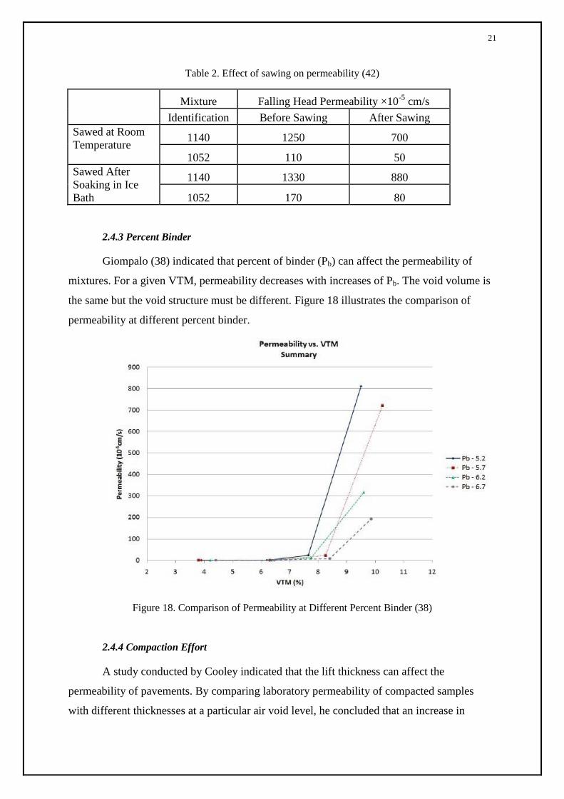
21
Table 2. Effect of sawing on permeability (42)
Mixture Falling Head Permeability ×10-5
cm/s
Identification Before Sawing After Sawing
Sawed at Room
Temperature 1140 1250 700
1052 110 50
Sawed After
Soaking in Ice
Bath
1140 1330 880
1052 170 80
2.4.3 Percent Binder
Giompalo (38) indicated that percent of binder (Pb) can affect the permeability of
mixtures. For a given VTM, permeability decreases with increases of Pb. The void volume is
the same but the void structure must be different. Figure 18 illustrates the comparison of
permeability at different percent binder.
Figure 18. Comparison of Permeability at Different Percent Binder (38)
2.4.4 Compaction Effort
A study conducted by Cooley indicated that the lift thickness can affect the
permeability of pavements. By comparing laboratory permeability of compacted samples
with different thicknesses at a particular air void level, he concluded that an increase in
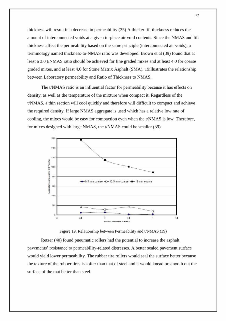
22
thickness will result in a decrease in permeability (35).A thicker lift thickness reduces the
amount of interconnected voids at a given in-place air void contents. Since the NMAS and lift
thickness affect the permeability based on the same principle (interconnected air voids), a
terminology named thickness-to-NMAS ratio was developed. Brown et al (39) found that at
least a 3.0 t/NMAS ratio should be achieved for fine graded mixes and at least 4.0 for coarse
graded mixes, and at least 4.0 for Stone Matrix Asphalt (SMA). 19illustrates the relationship
between Laboratory permeability and Ratio of Thickness to NMAS.
The t/NMAS ratio is an influential factor for permeability because it has effects on
density, as well as the temperature of the mixture when compact it. Regardless of the
t/NMAS, a thin section will cool quickly and therefore will difficult to compact and achieve
the required density. If large NMAS aggregate is used which has a relative low rate of
cooling, the mixes would be easy for compaction even when the t/NMAS is low. Therefore,
for mixes designed with large NMAS, the t/NMAS could be smaller (39).
Figure 19. Relationship between Permeability and t/NMAS (39)
Retzer (40) found pneumatic rollers had the potential to increase the asphalt
pavements’ resistance to permeability-related distresses. A better sealed pavement surface
would yield lower permeability. The rubber tire rollers would seal the surface better because
the texture of the rubber tires is softer than that of steel and it would knead or smooth out the
surface of the mat better than steel.

23
The literature suggests that several factors could affect the in-place permeability of
HMA pavements. Table 3 illustrates the factors that affect the in-place permeability
characteristics from research done across the United States:
2.5 Laboratory Permeability Test
2.5.1 Constant Head Permeability Test
Usually, the constant head test is performed to measure sand samples or permeable
asphalt samples. For instance, permeability of HMA mixtures designed to transmit water
should be measured by performing a constant head test (41). Testing samples can be saw cut
field cores or laboratory compacted pills, and the diameter of the specimen should be around
150 mm. A rubber membrane should be used to wrap the specimen, and porous stones should
be placed at the top and bottom. When water flows through the length of the specimen, both
Table 3. Factors that affect the in-place permeability
1. Air Voids Voids in total mix
Size of air voids
Percent of interconnected air voids
2. Aggregate
Aggregate Gradation
Nominal Maximum Aggregate Size
(NMAS) Percent material passing 0.6 mm sieve
Aggregate particle shape
3. Percent Binder (Pb)
4. Compaction Effort Lift thickness to NMAS ratio (t/NMAS)
The use of pneumatic rollers
Mixture temperature, rate of cooling
the inlet pressure and outlet pressure is controlled. Low differential inlet and outlet pressure
is required to achieve a laminar low (42). Figure 20 illustrates the constant head permeability
test on a highly permeable sand specimen.
The coefficient of permeability can be calculated using Equation2.6:
(2.6)

24
where:
K= permeability, cm/m;
Q= quantity of flow, cm3;
L= length of specimen, cm;
A= cross-sectional area of specimen, cm2;
t= interval of time over which flow Q occurs, s; and
h= difference in hydraulic head across specimen, cm.
Figure 20. Constant Head Permeability Device (42)
2.5.2 Falling Head Permeability Test
Based on Darcy’s Principle, the falling head permeability test is performed on low
permeable asphalt concrete or clay samples. Figure 21 illustrates the Karol-Warner falling
head permeability device. Water in a graduated cylinder is allowed to flow through a
saturated asphalt sample and the interval of time taken to reach a known change in head is
recorded. The coefficient of permeability can be calculated according to Equation 2.7.
(2.7)
where:
K= permeability, cm/m;
L= length of specimen, cm ;
A= cross-sectional area of cylinder, cm2;
t= time of flow between heads, s;
a= area of graduated cylinder, cm2;
h1= initial head of water, cm; and
h2= final head of water, cm.

25
Figure 21. Karol-Warner Falling Head Permeability Device (45)
A standard procedure, FM 5-565(43) for falling head permeability test was developed
by Florida Department of Transportation in 2000 and revised in 2006.
When performing laboratory permeability test following FM 5-565, it is assumed that
Darcy’s Law is valid, and applies to one-dimensional, laminar flow. Before performing
laboratory permeability test, the height of each core was measured at three locations recorded
to the nearest 0.5 mm. According to Florida Permeability Testing method, the maximum
difference in height of the three measurements for each core is 5 mm, any core exceeds this
tolerance should be discarded.
In order to reach a saturated condition, the sample was submerged into water for one
to two hours before performing laboratory permeability tests. One technique that aids in
achieving saturation is to fill the graduated cylinder with water and adjust the water inflow
equals to the outflow, and keep this condition for five to ten minutes. Next, the membrane
was inflated to 68.9±3.4 kPa (10±0.5 psi) to confine the core being tested, and maintain this
pressure through the test. Start the timing device when the bottom of meniscus of the water
reaches the upper time mark. The time it takes the water level to travel from the upper mark
to the lower mark is recorded as the elapsed test time. If a 4% or greater difference existed in
the three elapsed times was observed, this means the core being tested did not meet the
saturation requirement, and this test should be performed again. Considering the relationship
between temperature and water viscosity, a temperature of 20°Cis standardized by FDOT. A

26
temperature correction factor is used to adjust the water viscosity. The coefficient of
permeability can be calculated using Equation 2.8.
(2.8)
where:
K= permeability, cm/m;
L= length of specimen, cm;
A= cross-sectional area of cylinder, cm2;
t= time of flow between heads, s;
a= area of graduated cylinder, cm2;
h1= initial head of water, cm;
h2= final head of water, cm; and
tc= temperature correction for water viscosity.
Though the Florida Testing Method is widely used, Kanipong et al (7) found that this
testing method yielded variable and unrepeatable data. One potential cause can be short of
method to ensure the saturation state of samples. The maximum 4 percent difference between
two testing time of one sample required by the FM 5-565 does not ensure or control the
degree of saturation, and due to that, the permeability results obtained cannot be directly
applied to describe the capability of HMA to transmit fluid.
Compared to the constant head test, the falling head test is more suitable for laboratory
permeability tests because the falling head test is simple and capable of allowing water to
flow at a measureable pressure head. Sealant (petroleum jelly) is used to prevent water flow
along the sides of the specimen during the tests.
2.5.3 Acceptable Permeability Levels
A survey was conducted by Solaimanian to determine eight states’ approach in
dealing with the issue of permeability. The eight states included in the survey were Alabama,
Arkansas, Florida, Georgia, Minnesota, New Hampshire, Texas, and Virginia. Georgia and
Virginia use HMA permeability measurement as part of the mix design, and the remaining
six states use density as a measure of controlling permeability (41). The acceptable upper
limit for permeability in each of the eight states varies from 1×10⁻³
cm/sec to 1.5×10⁻³
cm/sec.
Table 4 illustrates the survey findings.

27
Table 4. Acceptable upper limit for permeability of five states
Agency Name Acceptable Permeability
Upper Limit (×10-3
)cm/sec
Florida Department of Transportation 1.25
Virginia Department of Transportation 1.50
Arkansas State Highway and Transportation Department 1.00
Georgia Department of Transportation 1.25
New England Transportation Consortium 1.00
2.5.4 Laboratory Pills versus Field Cores
Cooley et al (57) found differences in the permeability of laboratory pills versus field
cores, Figure 22. The laboratory pills were made from the same material as the field cores,
and were compacted to a range of air voids. Cooley et al concluded the trends between
permeability and air voids are different depending on the sample source. At less than 10
percent air voids the field samples have a higher permeability than lab cores. At greater than
10 percent air voids the slope of the curve fit to the lab pills is greater than the slope of the
field cores.
Figure 22. Permeability of Laboratory Pills versus Field Cores

28
2.6 Field Permeability Test
As a non-destructive method, field permeability testing describes a pavement’s
susceptibility to distresses commonly caused by water and air penetration, and has received a
growing concern from State transportation departments (4, 16, 32 and 45).Table 5 lists
advantages and disadvantages of the National Center for Asphalt Technology
(NCAT)Permeameter and the Kentucky Air Induced Permeameter (AIP). Few researches
were done on Kuss Constant Head Field Permeameter (KSHFP) and Romus Air Permeameter
(RAP).
2.6.1 NCAT Water Permeameter
The NCAT Permeameter, shown in Figure 23, is a falling head test which uses a
three-tier standpipe, with each tier having an increasing diameter from the top to the bottom
of the device. Water is stored within the standpipe and the rate of water flow out of the
standpipe and through the pavement is measured. When measuring the low permeable
pavement, the smallest diameter tier (top) is used to measure the rate of water fall. As the
permeability of pavement increases, the rate of water fall increases, and the larger diameter
tier should be used correspondingly (44).
Table 5. Advantages and disadvantages of NCATWP and AIP
Name Advantages Disadvantages
NCAT
Permeameter
A good performance
on level surface.
Enough time to
reach saturation.
Saturation affects the performance significantly
difficult to saturate low permeability pavement
within testing time.
Difficult to remove the silicon sealant after a
long time of using since it cured during the test.
Impossible to measure the permeability of super
elevated area because of the sliding of the gauge
on the pavement.
Large amount of water is required for multiple
tests.
AIP
It can be self-sealed
and testing time is
relative short (one
minute).
No supply of water
is required.
A gasoline operated air compressor or an
electrical generator is required to create a
vacuum of 68 psi.
A large compressor in the field may be
cumbersome.

29
Figure 23. NCAT Permeameter by Gilson Company. Inc., Model AP-1B
Water is allowed to remain in the bottom of the standpipe for at least one minute to
saturate the testing spots. When the water level is at the desired initial head, start the
stopwatch and stop the stopwatch when the water level within the standpipe reaches the
desired final head, record the initial head, final head, and the time interval that water takes to
drop from initial head to final head within the same standpipe tier. The coefficient of
permeability, K, is estimated using the Equation 2.7.
It should be noted that the result from the NCAT Water Permeameter are an index of
permeability rather than a true measurement. After water penetrates the pavement surface, it
can flow vertically and/ or horizontally which is against the assumption that there is only one
dimension flow exists. Without cutting the cores, the thickness and effective area of the
pavement that water flows through can only be assumed which can lead to inaccurate results.
Also, it is difficult to determine the degree of saturation of the underlying pavement.
Therefore, another parameter named infiltration rate was introduced.
In reality, water from the permeameter is not restricted to in-dimensional, and it can
flow in all three dimensions. The infiltration rate is the velocity or speed at which water
enters into the soil. In this study infiltration rate is a measure of the rate at which pavement is
able to absorb the water on the surface. Rather than permeability, a measure of infiltration
may be more appropriate (45). When performing the field permeability tests on longitudinal
joints using the NCAT Permeameter, based upon data collected, Williams et al found that the

30
computed permeability and infiltration value provided similar discrimination at joints with
different quality (46). The infiltration can be calculated using Equation 2.9.
(2.9)
where:
inf= the infiltration rate, cm/hr;
a= inside cross-sectional area of standpipe (cm
2);
h1= initial head (cm);
h2= final head (cm);
A= cross-sectional testing area (cm
2); and
t= elapsed time between h1 and h2, hr
2.6.2 Kuss Constant Head Field Permeameter
The KCHFP was developed by Mark L. Kuss in 2003,Figure 24. Based on constant
head method, this device uses a patented gas-measurement system to measure the amount of
air needed to replace the water to maintain a constant pressure head. When water from the
standpipe infiltrates the pavement testing surface approximately 1 inch, a sensor which is
connected to the flow meter box starts to monitor the water level. As water continues the
infiltration rate, the water level over the pavement drops, and the sensor alerts the flow valve.
The flow valve will allow air to enter the standpipe above the water column and the metered
volume of air acts as a substitute for the head pressure originally applied by the water to
maintain a constant head. The rate of water flow over time is automatically recorded by a
data acquisition system Figure 25 shows a schematic of the system.
The coefficient of permeability can be calculated using Equation2.10.
(2.10)
where:
K= coefficient of permeability, cm/s;
Q= flow rate, cm3/min;
A= area of base plate (1264.5 cm2); and
L= pavement thickness.

31
Figure 24. Kuss Field Permeameter (47)
Figure 25. Schematic of Kuss Field Permeameter
(47)
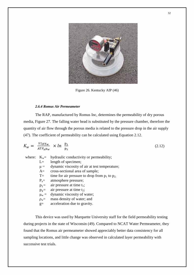
2.6.3 Kentucky Air Induced Permeameter
Developed by Kentucky Transportation Center, the AIP utilizes a vacuum, rather than
pressure to measure permeability, Figure 26. It is assumed that the smaller the voids spaces
are, the more difficult it is for the AIP to draw air through pavement, and the size and
percentage of voids are proportional to the permeability of pavement. The AIP uses an 8 inch
diameter testing area. Silicone-rubber is used as a sealant, and the sealing ring is 3 inches in
width to prevent air from “short-circuiting”. By using a vacuum, the AIP can be self-sealed.
By using multi-port venturi vacuum tube, the AIP is capable of forcing pressurized air at a
constant pressure of 68 psi. Air is drawn through the pavement, and the vacuum reading is
recorded automatically. The more difficult it is to draw air through the pavement, the lesser
the permeability is. Thus, high readings on the AIP represent low permeability (48). The
coefficient of permeability can be calculated as:
(2.11)
where:
k
=
permeability (ft/day); and
V
=
vacuum reading in mm Hg.
32
Figure 26. Kentucky AIP (46)
2.6.4 Romus Air Permeameter
The RAP, manufactured by Romus Inc, determines the permeability of dry porous
media, Figure 27. The falling water head is substituted by the pressure chamber, therefore the
quantity of air flow through the porous media is related to the pressure drop in the air supply
(47). The coefficient of permeability can be calculated using Equation 2.12.
(2.12)
where: Kw= hydraulic conductivity or permeability;
L= length of specimen;
μ = dynamic viscosity of air at test temperature;
A= cross-sectional area of sample;
T= time for air pressure to drop from p1 to p2;
Pa= atmosphere pressure;
= air pressure at time t1;
= air pressure at time t2;
μw = dynamic viscosity of water;
ρw= mass density of water; and
g= acceleration due to gravity.
This device was used by Marquette University staff for the field permeability testing
during projects in the state of Wisconsin (49). Compared to NCAT Water Permeameter, they
found that the Romus air permeameter showed appreciably better data consistency for all
sampling locations, and little change was observed in calculated layer permeability with
successive test trials.

33
Figure 27. Schematic of Romus Permeameter (40)
2.7 Mathematic Approach to the Permeability Estimation
The literature review indicates that permeability is an important property that
influences the performance of hot mix asphalt, and it is a function of several properties of
HMA such as percent binder, shape, size distribution and gradation of aggregate, and
compaction effort, etc. Currently, there is not a widely accepted device, procedure or
specification for measuring permeability of asphalt pavements, neither ASTM nor AASHTO
have a standard test method. Due to the multiple methods for permeability measurement
(both field and laboratory), and the presence of interaction among the influential factors, it is
difficult to develop an analytical equation that reflects the relationship between permeability
and all these factors.
Based on the well-known Kozeny-Carman equation, Masasd et al (50) developed an
empirical equation that utilizes the percent air voids and surface area of aggregates for
approximating the permeability of asphalt mixes. The surface area of air voids and aggregates
from field was collected by using X-ray CT images. The c, m and t values in Equation 2.13
are obtained through statistical data fitting to permeability values expressed in the units of
10-5
cm/sec.

34
(2.13)
where:
K= Permeability (m/s);
Va= Air voids of porous media (%);
m= Regression coefficient;
c= Constant that depends of the idealized shape of the air voids;
Sagg Average specific surface area of given gradation and NMAS (1/mm2);
γ= Unit weight of water at 20°C (9.79 kN/m3); and
μ= Viscosity of water (10-3
kg/m-s).
Westerman (51) developed an empirical equation that relates air voids and lift
thickness to the in-place permeability. Later, Equation 2.14 was applied by Haddock et al
(52)in a pavement failure investigation project to estimate the permeability on Indiana State
Road 38, and the permeability values obtained were confirmed by performing laboratory
permeability test at VTRC following the FM 5-565.
(2.14)
Where:
K= coefficient of permeability (cm/s);
AV= air voids (whole number); and
T= lift thickness (cm).
A research study was conducted by Louisiana Transportation Research Center
(LTRC). Field cores from 17 Superpave projects in Louisiana were sent to LTRC, and
permeability tests were performed using an LTRC modified version of Karol-Warner’s
falling-head permeameter. Mohammad et al (53) conducted a sensitivity analysis to relate the
permeability test results to the mixture air voids and gradation, and developed a statistical
regression model to predict the permeability of Superpave mixtures from the mixture
volumetric properties. The following equation was developed using multi linear regression
analysis:

35
(2.15)
where:
K= coefficient of permeability (mm/s);
AV= air voids;
P0.075= percent passing 0.075 mm sieve;
P0.3= percent passing 0.3 mm sieve;
P0.6= percent passing 0.6 mm sieve;
P2.36= percent passing 2.36 mm sieve;
P12.5= percent passing 12.5 mm sieve; and
L= height of specimen (mm).
Based on the principle explained by Taylor in 1956 in channel theory work for soils,
Vardanega and Waters derived representative pore size to help understand the parameters that
affect permeability (54). Related to the air voids and D754 of the asphalt mix grading curve,
the representative pore size is better correlated to the collected Superpave permeability data
than air voids. An equation was proposed to estimate the permeability of in-place pavements:
(2.16)
where:
K= coefficient of permeability in mm/s,
AV= percent air voids, %; and
D75= 75 percentile particle size, mm
Research by Vivar et al (55) indicated that air void content, aggregate size and
gradation significantly affect permeability. Both coarse-graded and fine-graded HMA
mixtures with 9.5 and 19.0 mm NMAS were compacted to 4, 6, 8 and 10 percent levels air
voids using a Superpave Gyration Compactor, and Florida Permeability tests were performed
on all samples. An exponential relationship was observed between air voids content and
permeability. By performing regression analysis, an equation was derived to investigate the
relationships of permeability and influential factors. An excellent goodness of fit (adjusted R2
of 0.93) was achieved for this equation:
4 D75 is the particle size that 75 percent of the particles have smaller diameters than it.

36
(2.17)
where:
K= Permeability (10-5 cm/s)
NMAS= Nominal Maximum Aggregate Size (mm)
VTM= Voids in the Total Mixture; and
Gradation= 0 for coarse-graded, 1 for fine-graded.

37
Chapter 3 Research Methodology
3.1 Introduction
This research consists of three parts:
1) Field permeability tests were conducted at four projects using NCAT Water
Permeameter. At three of the four projects, replicate permeability tests were conducted before
and after the application of polymer modified emulsion asphalt which was sprayed on the
pavement surface as a fog seal;
2) A total of 77 cores were removed from four construction projects and sent to the
Asphalt Technology Laboratory to perform density measurement and laboratory permeability
test; and
3) Eight HMA mixtures, a total of 64 laboratory compacted pills were produced to
perform laboratory permeability test.
3.2 Field Permeability Test
The field permeability testing device used in this study was developed by the National
Center for Asphalt Technology, and manufactured by Gilson Company, Inc., as described in
Section 2.6.1.
Putty is used to seal this device to the pavement surface. At the bottom there is a
flexible rubber mat and a hole cut to the diameter of the bottom tier standpipe. After the putty
is placed on the base plate, this unit is positioned on the test sites and gentle foot pressure is
applied to help seat the unit against the pavement. The flexible rubber is designed to assist the
foot pressure and base weight to push the putty into the pavement surface voids. When the
sealing process is done, a weight is then placed on the top of the base plate to resist the
hydrostatic uplift forces when the permeameter is filled with water and to provide a
downward force to maintain the sealing condition (42).
In this study, field permeability test were carried out at four locations: 1) Interstate 79
at mile post 75 in West Virginia, 2) Mon-Fayette Expressway, WV State Route 43, in the
north bound direction, right lane, approximately two miles from the Cheat Lake Exit, 3)
Quarry Run Road, and 4) Darnell Hollow Road and Seven Springs Road within Chestnut
Ridge Regional Part.

38
I-79 was a 1.5 inch overlay project and the measurements were performed on the left
lane, as Figure 28shown. At the time of the research, the Mon-Fayette was not opened to
traffic. The pavement structure was approximately eight years old, but was not opened to
traffic due to the sequential funding of the different parts of the project. While there was no
traffic damage to the pavement, the pavement was showing signs of oxidation and cracking.
The WV DOT decided to apply a fog seal of Blacklidge emulsions LD-7 to help preserve the
pavement surface. The infiltration rate was measured before and after the treatment to
evaluate the extent of sealing of the surface. Figure 29 and Figure 30 shows the application of
fog seal at Mon-Fayette and Quarry Run Road, and Figure 31 shows the pavement surface
condition before and after the application of fog seal.
Figure 28. Field Permeability Test Conducted at I-79 Project
The LD-7, polymer modified emulsion asphalt was sprayed on the pavement surface
at an application of 0.065gal/yd2 and the residual rate is 0.026 gal/yd
2. During the application,
the fog seal application appeared uniform.
Figure 29. Fog Seal Application at Mon-Fayette Project

39
Figure 30. Fog Seal Application at Quarry Run Road Project
Figure 31. Mon-Fayette Pavement Surface before and after the Fog Seal
3.3 Evaluation of Construction Projects
During this phase of the research, cores from construction projects on I-79, I-64, and
Route-19 were evaluated. Due to the nature of working with ongoing construction projects, it
was not feasible to design an experiment with selected factors and levels; rather, data and
samples were collected from the constructions on an “availability” basis. The bulk specific
gravity and permeability was evaluated for a variety of samples. The bulk specific gravity
was measured several different ways.

40
(1) On the I-79 project, milling followed by a1.5 inch overlay of Superpave 9.5 mm
skid resistant mix, the Gmb was measured using several methods:
a. Four contractor nuclear gauges,
b. Two WVDOH standard nuclear gauges,
c. A thin lift nuclear gauge on loan to the WVDOH
d. T 166 measured by the contractor, WVDOH, and in the WVUATL.
e. CoreLok measured by the contractor and in the WVUATL.
(2) On I-64 project, 24 cores were collected. 16 cores were 9.5 mm mix, and 8 cores
were 19 mm mix. The bulk specific gravity of these cores was measured by the
contractor using the CoreLok method. These cores were delivered to the WV ATL,
and Gmb was measured using CoreLok and T166 methods.
(3) On Route-19 project, 8 cores were collected for a Superpave 9.5 mm mix. Gmb
was measured with a CoreLok by the contractor. These cores were delivered to the
WVATL, and Gmb was measured using CoreLok and T166 methods.
After the density measurement, the samples were tested using a laboratory
permeameter following Florida Testing Method, “Testing Method for Measurement of Water
Permeability of Compacted Asphalt Paving Mixtures.
3.4 Laboratory Permeability of Gyratory Compacted Pills
3.4.1 Sample Preparation
Laboratory compacted pills were produced as a part of this study to evaluate how
aggregate gradation, NMAS and air voids content affects the permeability of Superpave
mixtures. Table 6 presents the factors and levels selected for the experimental design.
Table 6. Experimental design
Factors Levels
Mix Type 9.5, 12.5, 19, 25, 37.5 mm
NMAS Gradation Coarse and Fine
Air Voids
Content
4, 7, 9, 11 percent
A completed experimental design would require ten different mixes types. Due to
time considerations, two types were removed from the study: 12.5 mm fine and 25 mm
coarse. The contractor provided mix design for 6 mixes, 9.5 mm coarse, 12.5 mm coarse, 19
mm coarse and fine, 25 mm fine and 37.5 mm fine. For these mixes, the volumetric
properties were verified by preparing and testing samples at the WV ATL. Mix designs were
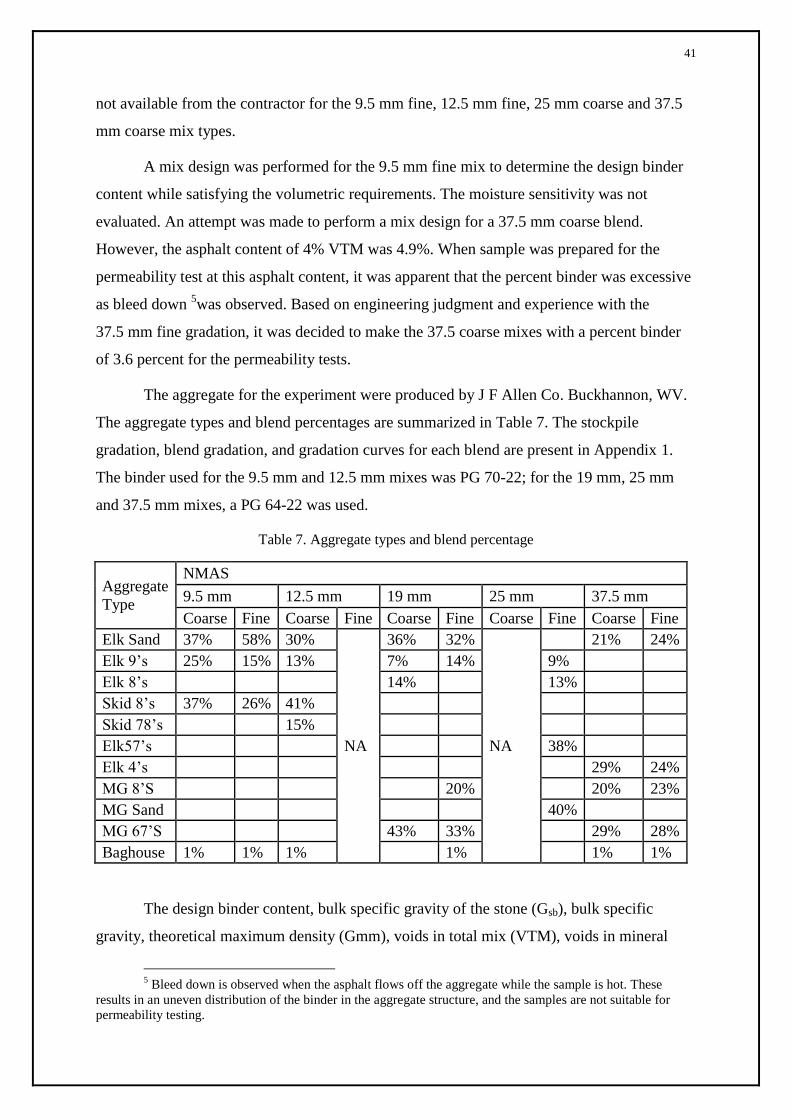
41
not available from the contractor for the 9.5 mm fine, 12.5 mm fine, 25 mm coarse and 37.5
mm coarse mix types.
A mix design was performed for the 9.5 mm fine mix to determine the design binder
content while satisfying the volumetric requirements. The moisture sensitivity was not
evaluated. An attempt was made to perform a mix design for a 37.5 mm coarse blend.
However, the asphalt content of 4% VTM was 4.9%. When sample was prepared for the
permeability test at this asphalt content, it was apparent that the percent binder was excessive
as bleed down 5was observed. Based on engineering judgment and experience with the
37.5 mm fine gradation, it was decided to make the 37.5 coarse mixes with a percent binder
of 3.6 percent for the permeability tests.
The aggregate for the experiment were produced by J F Allen Co. Buckhannon, WV.
The aggregate types and blend percentages are summarized in Table 7. The stockpile
gradation, blend gradation, and gradation curves for each blend are present in Appendix 1.
The binder used for the 9.5 mm and 12.5 mm mixes was PG 70-22; for the 19 mm, 25 mm
and 37.5 mm mixes, a PG 64-22 was used.
Table 7. Aggregate types and blend percentage
Aggregate
Type
NMAS
9.5 mm 12.5 mm 19 mm 25 mm 37.5 mm
Coarse Fine Coarse Fine Coarse Fine Coarse Fine Coarse Fine
Elk Sand 37% 58% 30%
NA
36% 32%
NA
21% 24%
Elk 9’s 25% 15% 13% 7% 14% 9%
Elk 8’s 14% 13%
Skid 8’s 37% 26% 41%
Skid 78’s 15%
Elk57’s 38%
Elk 4’s 29% 24%
MG 8’S 20% 20% 23%
MG Sand 40%
MG 67’S 43% 33% 29% 28%
Baghouse 1% 1% 1% 1% 1% 1%
The design binder content, bulk specific gravity of the stone (Gsb), bulk specific
gravity, theoretical maximum density (Gmm), voids in total mix (VTM), voids in mineral
5 Bleed down is observed when the asphalt flows off the aggregate while the sample is hot. These
results in an uneven distribution of the binder in the aggregate structure, and the samples are not suitable for
permeability testing.

42
aggregate (VMA), and voids filled with asphalt (VFA) for the eight mixes were summarized
in Table 8. The volumetric properties were evaluated for samples compacted with 80
gyrations of the SGC.
Table 8. Job mix formula values
Asphalt
(%) Gsb Gmb Gmm
VTM
(%)
VMA
(%)
VFA
(%)
9.5 Fine 4.9 2.640 2.393 2.494 4.0 13.8 70.6
19 Fine 4.9 2.660 2.408 2.500 3.7 13.9 73.5
25 Fine 5.0 2.647 2.405 2.491 3.5 13.7 74.7
37.5 Fine 3.8 2.669 2.419 2.531 4.4 12.8 65.5
9.5 Coarse 5.7 2.645 2.366 2.462 3.9 15.7 75.0
12.5 Coarse 5.2 2.647 2.381 2.482 4.1 13.8 73.4
19 Coarse 4.6 2.657 2.415 2.515 4.0 13.2 70.0
37.5 Coarse 3.6 2.672 2.449 2.533 NA
Samples used for permeability test were compacted using a SGC to a 75 mm height.
Gmb data of laboratory pills were measured using the T166. Gmm data were measured with the
AASHTO T209, and Gmm data provided by the contractor was verified, as well. The air voids
of all laboratory pills were computed using the contractor’s value for Gmm when available. A
±0.5% tolerance was selected for target air voids content of 4% and 7%, and ±1% tolerance
for target air voids content of 9% and 11%. Samples were rejected if they did not meet the
tolerance. At each target air voids content, there were two qualified samples prepared for the
laboratory permeability tests.
3.4.2Laboratory Permeability Tests on Gyratory Compacted Samples
The cylindrical samples were prepared for laboratory permeability following the
Florida Testing Method, FM 5-565. Compared with testing field cores, a thin layer of
petroleum jelly applied to the sides of the laboratory compacted samples is needed. The
petroleum jelly fills the large void son the sides of the specimen which are not representative
of the level of compaction of the interior of the specimen. The procedure described in Section
2.5.2 was used for testing. The temperature of water is kept constantly at 20°C through the
testing of the SGC pills. Equation 2.9 was used to calculate permeability.

43
3.5 Statistical Analysis Methods
The paired student test was selected to determine different Gmb measuring methods,
and performed by using Excel. The paired t test is appropriate when units are tested twice, a
“repeated measures” t test. The paired t test provides a hypothesis test of the difference
between population means for a pair of random samples, and the differences of the random
samples are approximately normally distributed. Hn, the null hypothesis, is defined as the
means of the populations from which the two samples were taken are equal, and the
alternative hypothesis, Ho, is for non-equal means. In this study, a confidence level of 95%
was selected for all the statistical analysis of the Gmb data collected. If two sided P-value
provided by the t-test is less than 0.05, then a decision can be made that there is sufficient
evidence to reject the Hn, which infers the data analyzed are not from the similar dataset. If
the two sided P-value is greater than 0.05, then there is insufficient evidence to reject the Hn,
which infers that the two data being compared are statistically the same.
A line of equality was used to better understand the relationship between the Gmb data
sets compared. If two test methods produce the same results, then when the two datasets were
plotted versus each other, a straight line with a slope of one and an intercept of zero should be
achieved. Equation 3.1 can be used to fit the two datasets that have a liner relationship. In this
study, a confidence level of 95% was applied, and at this level, the coefficients of the data
compared can be tested to determine if a=1 and b=0.
(3.1)
where:
a = the slope;
b= the intercept; and
e= the standard error.
The regression analysis function of Excel was used to compare the Gmb data, and a P-
value was picked from the results to determine if there was sufficient evidence to reject the
null hypothesis of the intercept equals to 0. A supplemental calculation procedure was used in
this study to test for a null hypothesis of the slope equals to 1 (56). The adjusted t-value for a
slope equal to 1 can be calculated in Equation 3.2. The P-value is computed using TDIST
function based upon the adjusted t-value, the residual degrees of freedom and the two tail
assumption as the arguments for the function.

44
( (3.2)

45
Chapter 4 Results and Analysis
4.1 Introduction
There are three distinct phases to this research, the field permeability tests, the
evaluation of materials from construction projects, and the laboratory investigation of
permeability. The evaluation of materials for the construction projects provides information
on both the measurement of Gmb and the permeability of pavements. These are treated as
separate issues in this chapter.
4.2 NCAT Permeameter Testing Results
As noted in Chapter 3, the NCAT Permeameter was used to evaluate infiltration at
four locations. While this was not a design experiment, some insight into the infiltration rates
under different pavement conditions can be gained by reviewing the data.
4.2.1 Interstate 79
The first attempt to use the permeameter was on Interstate 79. The contractor and WV
DOT were evaluating methods for establishing field calibration of nuclear density devices
using cores taken at the spot of nuclear density test. For this research, an attempt was made to
make the permeability measures after the nuclear measurements were collected but before the
cores were drilled for laboratory testing. Due to the contractor’s needs to drill the cores
shortly after the pavement was placed, the pavement surface was hot when the attempt was
made to measure infiltration. The temperature of the pavement surface adversely affected the
ability of the putty to seal the permeameter to the pavement surface. Consequently, water was
observed to leak between the pavement and the pavement surface, Figure 32. Several
attempts were made to resolve the leaking issue. The conclusion from the tests is the putty
sealed with the permeameter is not adequate when the pavement surface temperature is high.
4.2.2 Mon-Fayette Express Way
Table 9presents data collected on the Mon-Fayette project. The infiltration was
measured, and an average was computed. A second test was performed immediately
following curing of the fog seal, and data presents in Table 9indicates the fog seal was very
effective at reducing water penetration into the pavement, as the infiltration rate was reduced
by more than an order of magnitude.
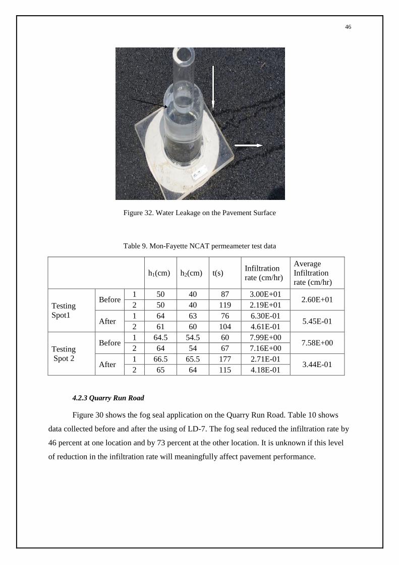
46
Figure 32. Water Leakage on the Pavement Surface
Table 9. Mon-Fayette NCAT permeameter test data
h1(cm) h2(cm) t(s) Infiltration
rate (cm/hr)
Average
Infiltration
rate (cm/hr)
Testing
Spot1
Before 1 50 40 87 3.00E+01
2.60E+01 2 50 40 119 2.19E+01
After 1 64 63 76 6.30E-01
5.45E-01 2 61 60 104 4.61E-01
Testing
Spot 2
Before 1 64.5 54.5 60 7.99E+00
7.58E+00 2 64 54 67 7.16E+00
After 1 66.5 65.5 177 2.71E-01
3.44E-01 2 65 64 115 4.18E-01
4.2.3 Quarry Run Road
Figure 30 shows the fog seal application on the Quarry Run Road. Table 10 shows
data collected before and after the using of LD-7. The fog seal reduced the infiltration rate by
46 percent at one location and by 73 percent at the other location. It is unknown if this level
of reduction in the infiltration rate will meaningfully affect pavement performance.

47
Table 10. Quarry Run Road NCAT permeameter data
h1(cm) h2(cm) t(s) Infiltration
rate (cm/hr)
Average
Infiltration
rate (cm/hr)
Testing
Spot1
Before 1 59 49 11 3.96E+04
7.56E+04 2 32 22 31 1.12E+05
After 1 33 23 50 1.80E+05
1.96E+05 2 33 23 59 2.12E+05
Testing
Spot 2
Before 1 33 23 23 8.28E+04
9.36E+04 2 33 23 29 1.04E+05
After 1 50 41 31 1.12E+05
2.59E+05 2 33 23 113 4.07E+05
4.2.4 Chestnut Ridge
The effectiveness of the fog seal cannot be properly assessed from the Chestnut Ridge
data as the infiltration rate of the pavement was not measured prior to the fog seal. It is not
known if the pavements at the Darnell Hollow road and Seven Spring locations were
sufficiently similar to allow a reasonable comparison. The data in Table 11are presented only
to document the work performed.
Table 11. Chestnut-Bridge NCAT permeability test data
h1(cm) h2(cm) t(s) Infiltration
rate (cm/hr)
Average
Infiltration rate
(cm/hr)
Testing
Spot1 Sealed
1 50 45 59 2.12E+05
2.52E+05 2 50 45 70 2.52E+05
3 44 39 81 2.92E+05
Testing
Spot 2 Unsealed
1 50 48 94 3.38E+05 3.15E+05
2 47.5 46 81 2.92E+05
4.3 Gmb Evaluation of Data for Construction Projects
As noted in Chapter 3 data were collected from construction projects on an
availability basis. Table 12 shows the types of data available for analysis. The actual data are
presented in Appendix 2. There are data for three projects, Interstate 79, Interstate 64, and
Route 19. Field density measurements are only available for the Interstate 79 project. Data
on the bulk specific gravity from cores, as measured by the contractor and the WVUATL are
available for all three projects.

48
4.3.1 Nuclear Gauge Measurements
Multiple nuclear gauge measurements were collected from the I79 project; nuclear
gauge measurements were not available for the other projects. As shown in Table 12 there
were two contractor’s nuclear gauges, four WVDOH nuclear gauges and a thin lift gauge
used on the project. Offset and centered measures were provided in some cases for the thin
lift gauge. Correction factors were developed for four dates. The two contractor’s gauges
were used for each control strip. The WVDOH and thin lift gauges used varied depending on
the date of the control strip.
Examination of Table 13 indicates:
The thin lift gauge had the smallest correction factor. In fact when the
contractor’s T166 Gmb values are used across all the available measurements
the correction factor for the offset thin lift gauge was zero.
For two dates, June 6 and August 2 control strips were performed both on the
joints and the mainline. The difference between the joint and mainline
correction factors ranged from 3 to 15 for the contractor’s gauges and 2 to 28
for the WVDOH gauges.
Based on the contractor’s T166 Gmb, the overall correction factor for the
contractor’s two gauges was -74 and -39 for gauges 35998 and 25500,
respectively. Overall the correction factors for the WVDOH gauges were
higher ranging from -76 to -115.
Comparing the correction factors for the CoreLok to the contractor’s T166
Gmb values shows the correction factors for the CoreLok are larger in
magnitude in all but one case. This indicates the CoreLok and T166 results
are different. This issue is more thoroughly evaluated later in this chapter.
Table 12. Nuclear density data available for analysis
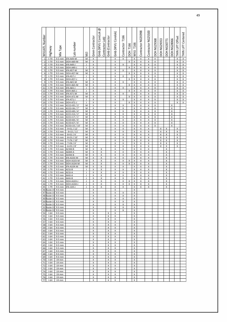
49
WV
UA
TL N
umbe
r
Hig
hway
Mix
Typ
e
Lab
num
ber
M/J
Gm
m C
ontr
acto
r
Gm
b (W
VU
Cor
eLok
@
Cont
ract
or L
ab)
Gm
b (C
ontr
acto
r
Gm
b (W
VU
Cor
elok
)
Cont
ract
or T
166
DO
H T
166
WV
U T
166
Cont
ract
or N
G35
998
Cont
ract
or N
G25
500
DO
H N
G29
368
DO
H N
G29
353
DO
H N
G30
771
DO
H N
G28
066
THIN
LIF
T O
ffse
t
THIN
LIF
T Ce
nter
ed
1 I-79 9.5 mm JFA-A49-M M X X X X X X X X X
2 I-79 9.5 mm DOH-A49-M M X X X X X X X X X
3 I-79 9.5 mm JFA-A49-J J X X X X X X X X X
4 I-79 9.5 mm DOH-A49-J J X X X X X X X X X
5 I-79 9.5 mm JFA-A57-M M X X X X X X X X X
6 I-79 9.5 mm DOH-A57-M M X X X X X X X X X
7 I-79 9.5 mm JFA-A57-J J X X X X X X X X X
8 I-79 9.5 mm DOH-A57-J J X X X X X X X X X
9 I-79 9.5 mm JFA-A65-M M X X X X X X X X X
10 I-79 9.5 mm DOH-A65-M M X X X X X X X X X
11 I-79 9.5 mm JFA-A65-J J X X X X X X X X X
12 I-79 9.5 mm DOH-A65-J J X X X X X X X X X
13 I-79 9.5 mm JFA-A71-M M X X X X X X X X X
14 I-79 9.5 mm DOH-A71-M M X X X X X X X X X
15 I-79 9.5 mm JFA-A71-J J X X X X X X X X X
16 I-79 9.5 mm DOH-A71-J J X X X X X X X X X
17 I-79 9.5 mm 4222+95 / 3' M X X X X X X X X
18 I-79 9.5 mm 4222+36 / 7' M X X X X X X X X
19 I-79 9.5 mm 4222+00 / 4' M X X X X X X X X
20 I-79 9.5 mm 4221+53 / 2' M X X X X X X X X
21 I-79 9.5 mm 4221+17 / 1' M X X X X X X X X
22 I-79 9.5 mm 4220+84 / 6' M X X X X X X X X
23 I-79 9.5 mm 4220+67 / 6' M X X X X X X X X
24 I-79 9.5 mm 4220+33 / 10' M X X X X X X X X
25 I-79 9.5 mm - 9+51 / 12' M X X X X X X X X X
26 I-79 9.5 mm - 9+15 / 11' M X X X X X X X X X
27 I-79 9.5 mm - 8+52 / 6' M X X X X X X X X X
28 I-79 9.5 mm - 8+23 / 10' M X X X X X X X X X
29 I-79 9.5 mm - 7+76 / 10' M X X X X X X X X X
30 I-79 9.5 mm - 7+56 / 6' M X X X X X X X X X
31 I-79 9.5 mm - 6+53 / 8' M X X X X X X X X X
32 I-79 9.5 mm A23M-B M X X X X X X X X
33 I-79 9.5 mm A44M-A M X X X X X X X X
34 I-79 9.5 mm A44M-B M X X X X X X X X
35 I-79 9.5 mm JFA-A103-M M X X X X X X X X
36 I-79 9.5 mm DOH-A103-M M X X X X X X X X X
37 I-79 9.5 mm DOH-A104-M M X X X X X X X X X
38 I-79 9.5 mm JFA-A104-M M X X X X X X X X
39 I-79 9.5 mm A23J-B J X X X X X X X X
40 I-79 9.5 mm A23J-A J X X X X X X X X
41 I-79 9.5 mm A44J-A J X X X X X X X X
42 I-79 9.5 mm A44J-B J X X X X X X X X
43 I-79 9.5 mm DOH-A103-J J X X X X X X X X X
44 I-79 9.5 mm DOH-A104-J J X X X X X X X X X
45 I-79 9.5 mm JFA-104-J J X X X X X X X X
46Route-19 9.5 mm X X X
47Route-19 9.5 mm X X X X
48Route-19 9.5 mm X X X X
49Route-19 9.5 mm X X X X
50Route-19 9.5 mm X X X X
51Route-19 9.5 mm X X X X
52Route-19 9.5 mm X X X X
53Route-19 9.5 mm X X X X
54 I-64 9.5 mm X X X X
55 I-64 9.5 mm X X X X
56 I-64 9.5 mm X X X X
57 I-64 9.5 mm X X X X
58 I-64 9.5 mm X X X X
59 I-64 9.5 mm X X X X
60 I-64 9.5 mm X X X X
61 I-64 9.5 mm X X X X
62 I-64 9.5 mm X X X X
63 I-64 9.5 mm X X X X
64 I-64 9.5 mm X X X X
65 I-64 9.5 mm X X X X
66 I-64 9.5 mm X X X X
67 I-64 9.5 mm X X X X
68 I-64 9.5 mm X X X X
69 I-64 9.5 mm X X X X
70 I-64 19 mm X X X X
71 I-64 19 mm X X X X
72 I-64 19 mm X X X X
73 I-64 19 mm X X X X
74 I-64 19 mm X X X X
75 I-64 19 mm X X X X
76 I-64 19 mm X X X X
77 I-64 19 mm X X X X

50
Table 13. Correction factor for nuclear gauges
Source Number
of cores
Contractor
Nuclear
Gauge
35998
Contractor
Nuclear
Gauge
25500
WV
DOH
Nuclear
Gauge
29368
WV
DOH
Nuclear
Gauge
29353
WV
DOH
Nuclear
Gauge
30771
WV
DOH
Nuclear
Gauge
28066
2220
THIN
LIFT
Offset
2220
THIN
LIFT
Centered
Corr
ecti
on F
acto
rs
from
Contr
acto
r
5/31/2011 mainline 8 -67 -27 -64 -76 20 20
6/6/2011 Joint 8 -65 -28 -87 21 27
mainline 8 -78 -31 -89 -1 -3
7/20/2011 mainline 8 -88 -57 -109 -128 -23
8/2/2011
Joint 8 -70 -42 -96
mainline 8 -85 -54 -124
combined 16 -88 -57 -128
WVU CoreLok -90 -55 -101 -111 -125 -100 -11 -8
Contractor T166 -74 -39 -80 -112 -115 -76 0 12

51
To evaluate the nuclear gauges data more thoroughly the line of equality plots were
prepared showing the nuclear gauge density versus laboratory measured density from cores
taken at the location where the density measurements were made. Figure 33, Figure 34 and
Figure 35 show the line of equality graphs for the contractor’s, WVDOH, and Thin Lift
gauges respectively. These graphs show there is a strong correlation between the nuclear
gauges and the bulk density from the CoreLok. However, there are differing amounts of
variance depending on the nuclear gauges as indicated by the goodness of fit statistic, R2.
Two trend lines were fit to each graph, one that best fits the data and one that forces
the intercept to zero. The coefficients and R2 results are summarized in Table 14. In general,
the intercept, b1, is fairly large, more than 100 in most cases. For the best fit equations the
slope varies from about 0.9 to 1.1. When the slope is not equal to 1.0, there is a divergence in
the comparative values, the further the x value is from the mean of the data set, the more error
there is in the prediction of the y value. For the trend lines that were forced to have an
intercept of zero, the slope is always less than one. As expected, the R2 is lower than for the
best fit equation, but the differences are relatively minor. The ratio of the average of the
dependent variable to the average of the independent variable, in this case the average
CoreLok to the average of the nuclear gauge readings, is equal to the slope of the regression
equation constrained to have a zero intercept. This suggest the correction factor developed
from control strips should be based on the ratio of the lab to field density, rather than the
difference of the means as is currently done. Figure 36 shows this concept. By using the ratio
method, the slope is closer to 1 and the intercept is closer to zero as compared to the
differences in means method. The R2 of the two methods is the same as there is no alteration
of the variability of the data.

52
Figure 33. Line of Equality Comparison for Contractor Gauges and CoreLok Density
y = 0.9145x + 107.02 R² = 0.7961
y = 0.9608x R² = 0.7941
2000
2050
2100
2150
2200
2250
2300
2350
2400
2000 2050 2100 2150 2200 2250 2300 2350 2400
WV
U C
ore
Lok
Contractor NG 35998
y = 1.0393x - 143.87 R² = 0.8287
y = 0.976x R² = 0.8256
2000
2050
2100
2150
2200
2250
2300
2350
2400
2000 2050 2100 2150 2200 2250 2300 2350 2400
WV
U C
ore
Lok
Contractor NG 25500

53
Figure 34. Line of Equality Comparison for WVDOH Gauges and CoreLok Density
y = 0.8872x + 161.82 R² = 0.7688
y = 0.9566x R² = 0.7641
2000
2050
2100
2150
2200
2250
2300
2350
2400
2000 2100 2200 2300 2400
WV
U C
ore
Lok
DOH NG 29368
y = 0.9654x - 32.551 R² = 0.8084
y = 0.9511x R² = 0.8082
2000
2050
2100
2150
2200
2250
2300
2350
2400
2000 2100 2200 2300 2400
WV
U C
ore
Lok
DOH NG 29353
y = 1.0903x - 335.39 R² = 0.8658
y = 0.9462x R² = 0.8507
2000
2050
2100
2150
2200
2250
2300
2350
2400
2000 2100 2200 2300 2400
WV
U C
ore
Lok
DOH NG 30711
y = 0.8869x + 164.41 R² = 0.904
y = 0.9573x R² = 0.8983
2000
2050
2100
2150
2200
2250
2300
2350
2400
2000 2100 2200 2300 2400
WV
U C
ore
Lok
DOH NG 28066

54
Figure 35. Line of Equality Comparison for Thin Lift Gauge and CoreLok Gmb
y = 0.9072x + 198.06 R² = 0.8533
y = 0.9957x R² = 0.8452
2000
2050
2100
2150
2200
2250
2300
2350
2400
2000 2050 2100 2150 2200 2250 2300 2350 2400
WV
U C
ore
Lok
THIN LIFT Offset
y = 0.8581x + 309.51 R² = 0.896
y = 0.9965x R² = 0.8727
2000
2050
2100
2150
2200
2250
2300
2350
2400
2000 2100 2200 2300 2400
WV
U C
ore
Lok
THIN LIFT Centered

55
Figure 36. Comparisons of Ratio and Difference of Means Methods for Correction Factors
corrected based on difference in means y = 0.9145x + 189.32
R² = 0.7961
uncorrected values y = 0.914x + 107.0
R² = 0.796
corrected based on ratio of means y = 0.9516x + 107.02
R² = 0.7961
1950
2000
2050
2100
2150
2200
2250
2300
2350
2400
2450
1950 2000 2050 2100 2150 2200 2250 2300 2350 2400 2450
De
nsi
ty f
rom
Co
reLo
k
NG 3598 Density
Corrected Uncorrected Ratio method
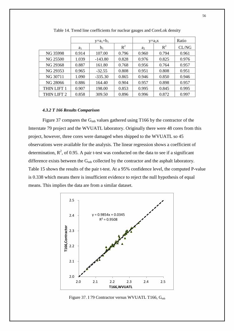
56
Table 14. Trend line coefficients for nuclear gauges and CoreLok density
y=a1+b1 y=a2x Ratio
a1 b1 R2 a2 R
2 CL/NG
NG 35998 0.914 107.00 0.796 0.960 0.794 0.961
NG 25500 1.039 -143.80 0.828 0.976 0.825 0.976
NG 29368 0.887 161.80 0.768 0.956 0.764 0.957
NG 29353 0.965 -32.55 0.808 0.951 0.808 0.951
NG 30711 1.090 -335.30 0.865 0.946 0.850 0.946
NG 28066 0.886 164.40 0.904 0.957 0.898 0.957
THIN LIFT 1 0.907 198.00 0.853 0.995 0.845 0.995
THIN LIFT 2 0.858 309.50 0.896 0.996 0.872 0.997
4.3.2 T 166 Results Comparison
Figure 37 compares the Gmb values gathered using T166 by the contractor of the
Interstate 79 project and the WVUATL laboratory. Originally there were 48 cores from this
project, however, three cores were damaged when shipped to the WVUATL so 45
observations were available for the analysis. The linear regression shows a coefficient of
determination, R2, of 0.95. A pair t-test was conducted on the data to see if a significant
difference exists between the Gmb collected by the contractor and the asphalt laboratory.
Table 15 shows the results of the pair t-test. At a 95% confidence level, the computed P-value
is 0.338 which means there is insufficient evidence to reject the null hypothesis of equal
means. This implies the data are from a similar dataset.
Figure 37. I 79 Contractor versus WVUATL T166, Gmb
y = 0.9854x + 0.0345 R² = 0.9508
2.0
2.1
2.2
2.3
2.4
2.5
2.0 2.1 2.2 2.3 2.4 2.5
T16
6,C
on
trac
tor
T166,WVUATL

57
Table 15. WVUATL versus Contractor T 166 paired t-Test
WVUATL
T166
Contractor
T166
Mean 2.230 2.232
Variance 0.004 0.004
df 44
P(T<=t) two-tail 0.338
Decision cannot reject Hn
The regression analysis comparing the contractor Gmb versus the laboratory Gmb using T 166
is shown in Table 16. At a confidence level of 95%, the p-value of the intercept, 0.081, is
greater than 0.05, the null hypothesis that the intercept is equal to 0 cannot be rejected,
inferring that the computed intercept is statistically equal to 0. The p-value of the slope, 0.108,
is greater than 0.05, the null hypothesis that the slope is equal to 1 cannot be rejected,
inferring that the computed slope is statistically equals to 1.
Table 16. WVUATL versus contractor T166 Regression Analysis
Regression Statistics
Multiple R 0.943
R Square 0.890
Adjusted R Square 0.887
Standard Error 0.021
Observations 45
ANOVA
df SS MS F
Regression 1 0.156 0.156 347.891
Residual 43 0.019 0.000 Total 44 0.175
Coefficients Std Error t Stat P-value
Intercept 0.195 0.109 1.787 0.081
X Variable 1 0.919 0.049 18.652 0.000
tails 2 Decision
t for Hn = 1 -1.642 Intercept cannot reject Hn
p-value for Hn = 1 0.108 Slope cannot reject Hn
Both the t-test and the regression analysis demonstrate the T166 tests performed on
the cores from construction projects indicate the WVUATL and the contractor produced
statistically similar results.

58
4.3.3 CoreLok Gmb Results Comparisons
During the Interstate 79 project the WVUATL the CoreLok and CoreDry equipment
were transported to the contractor’s lab to demonstrate the equipment. Gmb was measured on
14 cores. These cores were subsequently transported to the WVUATL and retested. The
results of the t-test are presented in Appendix 3; the relevant statistics for the paired t-test
comparison of these data are (Table 17):
Table 17. Statistics for the paired t-test comparison of these data
Mean Variance df p-value Decision
WVUATL 2.219 0.005 13 3.64E-05 reject Hn
I-79 Contractor Lab 2.226 0.004
The decision is to reject the hypothesis of equal means. This is a situation where the
variances of the tests is so small that even a minor difference in the means of the two
populations results in the decision to reject the null hypothesis. The practical conclusion of
this comparison is the populations are similar, and the t-test conclusion results from the
abnormally small variances of the population.
The trend line equation is shown on Figure 38. The regression analysis statistics in
Appendix 3 demonstrate the null hypotheses of zero and one for the intercept and slope,
respectively, cannot be rejected, indicating the data are from statistically similar populations.
The contractor for the Interstate 64 project provided 24 cores and Gmb CoreLoK
measurements. The cores were retested at the WVUATL. The results of the t-test are
presented in Appendix 3; with the relevant statistics for the paired t-test presented in Table 18.
The decision is to reject the hypothesis of equal means.
Table 18. Statistics for the paired t-test comparison of these data
Mean Variance df p-value Decision
WVUATL CoreLok 2.299 0.017 23 1.35E-02 reject Hn
Contractor CoreLok 2.274 0.013
Figure 39 presents the trend line equation. The regression analysis statistics in
Appendix 3 demonstrate the null hypotheses of zero and one for the intercept and slope,
respectively, can be rejected, indicating the data are from statistically different populations,
supporting the conclusion from the t-test. Figure 37 compared to Figure Figure 39 shows the
variability across two machines and labs was greater than the variability for a single machine,
as is expected.

59
Figure 38. Comparison of WVUATL CoreLok Replicated Testing Results
Figure 39. WVUATL versus Contractor CoreLok Results
y = 0.9864x + 0.0368 R² = 0.9964
2.1
2.2
2.3
2.4
2.5
2.1 2.2 2.3 2.4 2.5
Co
reLo
k G
mb,W
VU
ATL
CoreLok Gmb ,WVUATL
y = 1.0804x - 0.1577 R² = 0.8832
2.1
2.2
2.3
2.4
2.5
2.6
2.1 2.2 2.3 2.4 2.5 2.6
Co
reLo
k G
mb
, Co
ntr
acto
r
CoreLok Gmb, WVUATL

60
4.3.4 CoreLok versus T166
The preceding analysis demonstrated that the contractor and the WVUATL produced
similar T 166 results. Therefore the following analysis used the WVUATL Gmb data for the
comparison between CoreLok and T 166. According to T 166, when the percent of water
absorbed by the specimen exceeds 2%, AASHTO T 275 or T 331 should be used to
determine the bulk specific gravity. There is a proposal to reduce this threshold to one percent.
Hence the following analysis considers these different threshold values. Figure 40shows the
line of equality for the data from the 77 cores with different symbols based on the threshold
of absorption. One can observe that in general there is an inverse trend between absorption
and specific gravity; the samples with less than one percent absorption have higher specific
gravity than the other samples. This is logical as the samples with low absorption would also
have low air voids and therefore higher specific gravity. It can also be observed that the
samples with less than one percent absorption are on both sides on the line of equality while
the preponderance of samples with more than one percent absorption are above the line of
equality.
Figure 40. WVUATL CoreLok versus T 166.
2.0
2.1
2.2
2.3
2.4
2.5
2.0 2.1 2.2 2.3 2.4 2.5
T 1
66
Gm
b, W
VU
ATL
CoreLok Gmb, WVUATL
Water Absorption, <1%
Water Absorption, 1 to 2%
Water Absorption >3%

61
The complete results of the t-tests and regression analysis are presented in Appendix 3.
Table 19 is a summary of the statistical results. The t-test and regression analysis are in
agreement. The null hypothesis is not rejected is when the absorption is less than one percent
and less than two percent. In all other cases the null hypothesis is rejected. This analysis
supports the proposed change to T 166 to limit the its use to samples with less than one
percent absorption and use the vacuum method, T 331, in all other cases.
Table 19. Statistical comparison of CoreLok and T166
Absorption threshold
Parameters All <1% ≧1% <2% ≧2%
pai
r t-
test
Mean CoreLok 2.238 2.327 2.193 2.286 2.159
Mean T166 2.247 2.324 2.207 2.289 2.177
Variance CoreLok 0.010 0.006 0.006 0.007 0.005
Variance T166 0.008 0.005 0.004 0.006 0.003
df 76 25 50 47 28
P-value 8.25E-03 6.53E-01 2.18E-04 3.91E-01 1.96E-03
decision reject Hn cannot
reject Hn reject Hn
cannot
reject Hn reject Hn
regre
ssio
n a
nal
ysi
s
R2 0.920 0.849 0.877 0.885 0.868
a1 0.854 0.963 0.829 0.855 0.776
P-value 3.64E-02 7.82E-02 3.50E-04 2.59E-03 2.04E-03
decision reject Hn cannot
reject Hn reject Hn reject Hn reject Hn
b1 0.335 0.314 0.387 0.334 0.500
P-value 2.83E-02 8.07E-02 2.19E-04 2.37E-03 1.49E-03
decision reject Hn cannot
reject Hn reject Hn reject Hn reject Hn
4.4 Laboratory permeability test results of field cores
One of the primary goals of this research was to evaluate the relationship between
laboratory permeability and in-place density. Laboratory permeability tests were performed
on 45 field cores from I-79, 24 from I-64, and 8 from Route-19. The air voids content were
determined based upon the bulk specific gravity of cores measured by T166 and maximum
theoretical specific gravities supplied by the contractors for plant-produced mix.

62
4.4.1 Permeability analysis of I-79 Cores
Figure 41 presents the data for the laboratory permeability and percent air voids for the cores
from I-796. The coefficient of determination, R
2, of 0.883 indicates that most of the variation
in permeability is attributed the percent air voids. At percent air voids below 6 percent, the
permeability is very low. The permeability increases at a greater rate with changes in percent
air voids from 6 to 8 percent air voids. At percent air voids above 8 percent, small changes in
air voids leads to a large increases in permeability.
Figure 41. Relationship between Permeability and Air Voids Content~I-79 Project
Inspection of Figure 41 demonstrates that in general the percent air voids of the cores
are greater than the percent air voids of the mainline cores. The higher air voids is associated
with higher permeability which is in turn associated with accelerated pavement deterioration.
The commonly accepted criterion for permeability is 100x10-5
to 125x10-5
cm/s, Table 4,
6 The percent air voids was 17% for one core. This is sufficiently high to trigger concern that the tests were
performed correctly. However, tests by the contractor, and the WVUATL using both the CoreLok and T 166
were all in agreement.
y = 5E-05x6.5789 R² = 0.883
0
200
400
600
800
1,000
1,200
1,400
1,600
4.0 6.0 8.0 10.0 12.0 14.0
Pe
rme
abili
ty ×
10
-5 c
m/s
ec
Percent Air Voids
Longitudinal Joints
Mainline

63
which corresponded to approximately 8 percent air voids. 13 out of 15 longitudinal samples
and 16 out of 30 mainline samples have the air voids content greater than 8 percent.
4.4.2 Permeability analysis of I-64 and Route-19 Projects
Figures 42 and 43 illustrate the permeability-density relationship for the cores
collected from I-64 and Route-19, respectively. Two 9.5 mm cores from I-64 project have
high percent air voids content and correspondingly high permeability. The power functional
form was used for modeling the other comparisons as this is the functional form most
commonly used in the literature. However, as shown on Figure 42 the exponential functional
form does a better job of capturing the rapid increase in permeability with air voids for this
data set.
Figure 42. Relationship between Permeability and Air Voids ~I-64 Project
Figure 43 shows the percent air voids versus permeability for the 9.5 mm mix used on
Route 19. For a given level of air voids this mix has a much lower permeability than the
other mixes both in this study and in the literature. The reason for this anomaly is unknown.
4.4.3 Composite Analysis of Samples from All Construction Projects
Figure 44 has the permeability – percent air void data for all the projects. As
expected the amount of scatter is greater than for the analysis of the individual projects.
y = 2.3908e0.4172x R² = 0.7569
y = 0.5087x2.6078 R² = 0.7346
0
1,000
2,000
3,000
4,000
5,000
6,000
0.0 5.0 10.0 15.0 20.0
Pe
rme
abili
ty ×
10
-5 c
m/s
ec
Percent Air Voids
I-64 9.5 mm
I-64 19 mm

64
However, the R2values for both the power and the exponential functions are reasonable. As
was the case for the I-64 analyses, the exponential model appears to capture the extreme
permeability values better than the power function. Cooley et al. (57) reported a R2 of 0.69
for a power equation fit of field permeability and percent air voids. As shown on Figure 44
the Cooley equation predicts higher permeability than the data from this study. This may be
due to the fact that the NCAT Permeameter used by Cooley allows three dimensional flows
versus the one dimensional flow of the permeameter used in this study. Hainin et al. (35)
tested field cores using the Florida method. Figure 44 shows Hainin’s equation falls between
the Cooley’s and the one developed in this study. The R2 of Hainin’s equation was 0.501.
Figure 43. Relationship between Permeability and Density~Route-19 Project
y = 7E-10x10.086 R² = 0.8524
0
500
1,000
1,500
2,000
2,500
3,000
3,500
4,000
0.0 5.0 10.0 15.0 20.0
Pe
rme
abili
ty ×
10
-5 c
m/s
ec
Percent Air Voids
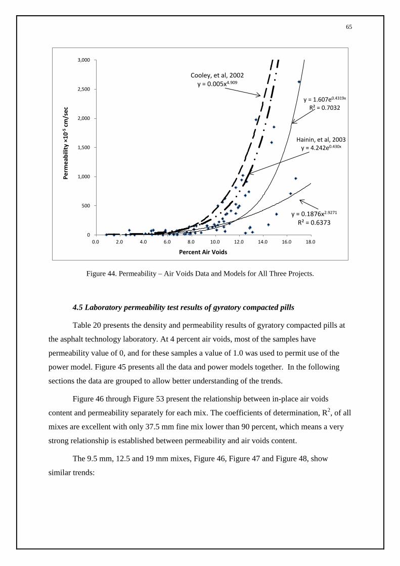
65
Figure 44. Permeability – Air Voids Data and Models for All Three Projects.
4.5 Laboratory permeability test results of gyratory compacted pills
Table 20 presents the density and permeability results of gyratory compacted pills at
the asphalt technology laboratory. At 4 percent air voids, most of the samples have
permeability value of 0, and for these samples a value of 1.0 was used to permit use of the
power model. Figure 45 presents all the data and power models together. In the following
sections the data are grouped to allow better understanding of the trends.
Figure 46 through Figure 53 present the relationship between in-place air voids
content and permeability separately for each mix. The coefficients of determination, R2, of all
mixes are excellent with only 37.5 mm fine mix lower than 90 percent, which means a very
strong relationship is established between permeability and air voids content.
The 9.5 mm, 12.5 and 19 mm mixes, Figure 46, Figure 47 and Figure 48, show
similar trends:
y = 0.1876x2.9271 R² = 0.6373
y = 1.607e0.4319x R² = 0.7032
Cooley, et al, 2002 y = 0.005x4.909
Hainin, et al, 2003 y = 4.242e0.430x
0
500
1,000
1,500
2,000
2,500
3,000
0.0 2.0 4.0 6.0 8.0 10.0 12.0 14.0 16.0 18.0
Pe
rme
abili
ty ×
10
-5 c
m/s
ec
Percent Air Voids

66
Table 20. Density and permeability results
9.5
mm
Fin
e Air Voids (%)
Permeability
(E-5 cm/s)
9.5
mm
Coar
se
Air Voids (%) Permeability
(E-5 cm/s)
3.9 0 4.1 0
4.0 0 4.1 0
7.1 11.4 6.9 2.1
7.1 19.2 7.3 2.3
9.0 75.2 8.7 95.9
9.5 84.7 8.9 92.7
10.7 112.2 11.2 573.9
11.7 180.9 11.5 441.6
12.5
mm
Coar
se
4.1 0
19.5
mm
Fin
e
3.8 0
4.3 0 4.3 0.1
7.2 3.4 6.6 1.1
7.5 6.8 7.0 5.9
8.8 109.4 8.5 73.3
8.9 68.2 8.8 85.7
11.4 928.5 10.2 676.7
11.8 686.9 11.9 1294.7
19.5
mm
Coar
se
4.2 0
25 m
m F
ine
3.7 0
4.5 0.2 4.2 0
6.6 68 7.2 61
7.2 50.9 7.4 98.5
8.6 195.1 9.3 536.4
8.7 308.8 9.8 187
10.0 1103.6 10.5 1012.7
10.2 1704.7 11.1 1498.5
37.5
mm
Fin
e
3.6 0
37.5
mm
Coar
se
3.2 0
4.4 30.7 4.5 0
7.0 1180.9 7.5 934.9
7.1 1121.9 7.8 1036.4
8.5 1869.8 9.0 2493.1
8.5 1980.7 9.3 3451.9
9.3 2449.3 10.3 3134.1
10.4 2639.7 11.0 4351.5

67
Figure 45. Permeability and Percent Air Voids Value of Eight HMA Mixes
9.5 mm Fine y = 7E-06x7.192
R² = 0.976
9.5 mm Coarse y = 8E-07x8.233
R² = 0.934
12.5 mm Coarse y = 5E-07x8.571
R² = 0.966
19 mm Fine y = 2E-07x9.080
R² = 0.952
19 mm Coarse y = 5E-08x10.49
R² = 0.976
25 mm Fine y = 2E-06x8.624
R² = 0.973
37.5 mm Fine y = 1E-05x8.842
R² = 0.853
37.5 mm Coarse y = 4E-07x10.08
R² = 0.935
0
500
1,000
1,500
2,000
2,500
3,000
3,500
4,000
4,500
5,000
0 2 4 6 8 10 12
Lab
Pe
rme
abili
ty E
-5 c
m/s
ec
Percent Air Void
9.5 mm Fine9.5 mm Coarse12.5 mm Coarse19.5 mm fine19.5 mm Coarse25 mm Fine37.5 mm Fine37.5 mm CoarsePower (9.5 mm Fine)Power (9.5 mm Coarse)Power (12.5 mm Coarse)Power (19.5 mm fine)Power (19.5 mm Coarse)Power (25 mm Fine)Power (37.5 mm Fine)Power (37.5 mm Coarse)
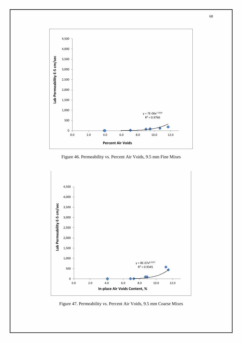
68
Figure 46. Permeability vs. Percent Air Voids, 9.5 mm Fine Mixes
Figure 47. Permeability vs. Percent Air Voids, 9.5 mm Coarse Mixes
y = 7E-06x7.1924 R² = 0.9766
0
500
1,000
1,500
2,000
2,500
3,000
3,500
4,000
4,500
0.0 2.0 4.0 6.0 8.0 10.0 12.0
Lab
Pe
rme
abili
ty E
-5 c
m/s
ec
Percent Air Voids
y = 8E-07x8.2337 R² = 0.9345
0
500
1,000
1,500
2,000
2,500
3,000
3,500
4,000
4,500
0.0 2.0 4.0 6.0 8.0 10.0 12.0
Lab
Pe
rme
abili
ty E
-5 c
m/s
ec
In-place Air Voids Content, %

69
Figure 48. Permeability vs. Percent Air Voids, 12.5 Coarse Mixes
Figure 49. Permeability vs. Percent Air Voids, 19 mm Fine Mixes
y = 5E-07x8.5711 R² = 0.9665
0
500
1,000
1,500
2,000
2,500
3,000
3,500
4,000
4,500
0.0 2.0 4.0 6.0 8.0 10.0 12.0
Lab
Pe
rme
abili
ty E
-5 c
m/s
ec
Percent Air Voids
y = 2E-07x9.0803 R² = 0.9526
0
500
1,000
1,500
2,000
2,500
3,000
3,500
4,000
4,500
0.0 2.0 4.0 6.0 8.0 10.0 12.0
Lab
Pe
rme
abili
ty E
-5 c
m/s
ec
Percent Air Voids

70
Figure 50. Permeability vs. Percent Air Voids, 19 mm Coarse Mixes
Figure 51. Permeability vs. Percent Air Voids, 25 mm Fine Mixes
y = 5E-08x10.49 R² = 0.976
0
500
1,000
1,500
2,000
2,500
3,000
3,500
4,000
4,500
0.0 2.0 4.0 6.0 8.0 10.0 12.0
Pe
rme
abili
ty E
-5 c
m/s
ec
Percent Air Voids
y = 2E-06x8.6246 R² = 0.973
0
500
1,000
1,500
2,000
2,500
3,000
3,500
4,000
4,500
0.0 2.0 4.0 6.0 8.0 10.0 12.0
Pe
rme
abili
ty E
-5 c
m/s
ec
Percent Air Voids

71
Figure 52. Permeability vs. Percent Air Voids, 37.5 mm Fine Mixes
Figure 53. Permeability vs. Percent Air Voids, 37.5 mm Coarse Mixes
y = 1E-05x8.8426 R² = 0.8533
0
500
1,000
1,500
2,000
2,500
3,000
3,500
4,000
4,500
0.0 2.0 4.0 6.0 8.0 10.0 12.0
Pe
rme
abili
ty E
-5 c
m/s
ec
Percent Air Voids
y = 4E-07x10.08 R² = 0.9355
0
500
1,000
1,500
2,000
2,500
3,000
3,500
4,000
4,500
0.0 2.0 4.0 6.0 8.0 10.0 12.0
Pe
rme
abili
ty E
-5 c
m/s
ec
Percent Air Voids

72
4.5.1 Relationship between Permeability and Percent Air Voids
at air voids below 6 percent, the samples were impermeable,
from 6 to 7 percent, the permeability started to increase with the increase of
air voids content, and
at air voids level above 8 percent permeability increases sharply with small
increase in in-place air voids content.
Cooley et al. (32) reported similar observations for 9.5 and 12.5 mm mixes.
Figure 49 and Figure 50 illustrate the relationship between laboratory permeability
and in-place air voids for 19 mm NMAS fine and coarse mixes. The permeability is typically
low at low air voids content, and it increases with the increase of air voids content. Above 7
percent, a small change in air voids content results in a large increase in permeability.
Figure 51 illustrates the relationship between permeability and in-place air voids for
25 mm NMAS fine mix. In this study, only 25 mm fine-graded mix was prepared, and data in
Figure 51suggests that 25 mm fine-graded Superpave mix can be excessive permeable above
7 percent in-place air voids. Cooley et al. (32) suggested 4.4 percent in-place air voids should
be a threshold for 25 mm coarse-graded Superpave mixes.
Figure 52and Figure 53 show the relationship between permeability and in-place air
voids for 37.5 mm NMAS fine and coarse mixes. The samples are impermeable with air
voids level lower than approximately 4.5 percent. For 37.5 mm fine-graded and coarse-
graded, when the air voids were higher than 5 and 6 percent, the permeability values
increased significantly with small changes in in-place air voids content. The maximum
permeability value obtained in this study is 4350 cm/sec from a 37.5 mm NMAS coarse-
graded sample with 11 percent in-place air voids.
The upper limit of in-place air voids for constructing an impermeable 9.5 and 12.5
mm NMAS HMA mixes is approximately 8 percent(55). Table 21 presents the permeability
value of all eight HMA mixes based upon the 8 percent air voids threshold. The 9.5 mm fine
and coarse, 12.5 mm coarse and 19 mm fine mixes meet the requirement with permeability
value lower than 1×10⁻³
cm/sec at eight percent air voids. The 19 mm coarse, 25 mm fine,
37.5 mm fine and coarse mixes have permeability greater than 1×10⁻³
cm/sec at 8 percent air
voids. Using the 8 percent criteria for these mixes would result in pavement with
unacceptable high permeability.

73
Table 21. Permeability value at eight percent air voids
NMAS (mm) Gradation Air Voids,
percent
Permeability
(10-5 cm/sec)
9.5 Fine 8 22
9.5 Coarse 8 22
12.5 Coarse 8 28
19 Fine 8 32
19 Coarse 8 149
25 Fine 8 123
37.5 Fine 8 966
37.5 Coarse 8 507
The original upper limit permeability value used by FDOT for quality-control was
1×10⁻³
cm/sec and was later increased to 1.25×10⁻³
cm/sec, as cited by Maupin (42). VDOT
requires a permeability value of 1.5×10⁻³
cm/sec or less at 7.5 percent air voids as cited
Maupin (29). Table 22 presents the air voids value for eight HMA mixes at 1×10⁻³
and
1.25×10⁻³
cm/sec permeability based on the relationship plotted on Figure 46 through Figure
53.
If 1×10⁻³
cm/sec is selected as the permeability threshold, then the 9.5 mm fine and
coarse, 12.5 mm coarse, and 19 mm fine HMA mixes would meet the air voids content
requirement at eight percent air voids. If 1.25×10⁻³
cm/sec is chosen as the criterion, then 37.5
mm fine and coarse mixes need to be compacted to initial air voids of approximately 6 to 7
percent.
4.5.2 Relationship between permeability and Gradation of HMA mixes
The data plotted in Figure 54 through Figure 56 illustrate how aggregate gradation
affects the permeability. Literature review indicates that the permeability of HMA mixtures
cannot be controlled by air voids content alone, it also depends on the aggregate gradation. At
a similar air voids content, coarse-graded Superpave mixes appear to be more permeable than
conventional dense-graded mixes (7).
Figure 54 illustrates the relationship between permeability and in-place air voids for
9.5 mm fine and coarse mixes. It is observed that the permeability value is similar at low in-
place air voids value. At air voids approximately above 8 percent, the permeability of coarse
mix started to increase faster than the fine mix with twice higher permeability value at 10
percent air voids level and three times higher than fine mix at 11 percent air voids level.

74
Table 22. Air voids content corresponding to select permeability values
NMAS
(mm) Gradation Permeability Air voids,
percent Permeability
Air
voids,
percent (E-5 cm/sec) (E-5 cm/sec)
9.5 Fine 100 9.9 125 10.2
9.5 Coarse 100 9.6 125 9.9
12.5 Coarse 100 9.3 125 9.5
19 Fine 100 9.1 125 9.3
19 Coarse 100 7.7 125 7.9
25 Fine 100 7.8 125 8.0
37.5 Fine 100 6.2 125 6.3
37.5 Coarse 100 6.8 125 7.0
Figure 54. Permeability versus Percent Air Voids, 9.5 mm Fine and Coarse Mixes
y = 7E-06x7.1924 R² = 0.9766
y = 8E-10x11.31 R² = 0.9198
0
100
200
300
400
500
600
700
800
900
0.0 2.0 4.0 6.0 8.0 10.0 12.0
Lab
Pe
rme
abili
ty E
-5 c
m/s
ec
Percent Air Voids
9.5 mm Fine-graded
9.5 mm Coarse-graded
Power (9.5 mm Fine-graded)
Power (9.5 mm Coarse-graded)

75
Figure 55. Permeability versus Percent Air Voids, 19 mm Fine and Coarse Mixes
Figure 56. Permeability versus Percent Air Voids, 37.5 mm Fine and Coarse Mixes
y = 5E-08x10.49 R² = 0.976
y = 2E-07x9.0803 R² = 0.9526
0
200
400
600
800
1,000
1,200
1,400
0.0 2.0 4.0 6.0 8.0 10.0 12.0
Lab
Pe
rme
abili
ty E
-5 c
m/s
ec
Percent Air Voids
19 mm Coarse-graded
19 mm Fine-graded
Power (19 mm Coarse-graded)
Power (19 mm Fine-graded)
y = 4E-07x10.08 R² = 0.9355
y = 1E-05x8.8426 R² = 0.8533
0
500
1,000
1,500
2,000
2,500
3,000
3,500
4,000
0.0 2.0 4.0 6.0 8.0 10.0 12.0
Lab
Pe
rme
abili
ty E
-5 c
m/s
ec
Percent Air Voids
37.5 mm Coarse-graded
37.5 mm Fine-graded
Power (37.5 mm Coarse-graded)
Power (37.5 mm Fine-graded)

76
Figure 55 illustrates how aggregate gradation affects the permeability characteristics
of 19 mm NMAS HMA mixes. At 4 percent in-place air voids content, both fine and coarse-
graded mixes have low permeability values. Above 5.5 percent air voids, the permeability
started to increase. The coarse-graded mix became excessive permeable much faster than the
fine-graded mix.
Figure 56 illustrates the relationship between permeability and in-place air voids for
37.5 mm fine-graded and coarse-graded mixes. As the trend lines show, the fine-graded mix
reached the permeability threshold earlier than the coarse-graded mix, and this can be caused
by the data obtained from samples at approximately 7 percent air voids. Based upon data in
Figure 56, the coarse-graded mix has higher permeability than fine-graded mix with in-place
air voids above 8 percent. At high air voids level, the difference between 37.5 mm fine-
graded and coarse-graded mixes was not as obvious as the ones obtained from 9.5 mm and 19
mm mixes.
4.5.3 Relationship between permeability and NMAS
Based upon NMAS and aggregate gradation, the eight different HMA mixes were
arranged on Figure 57 to show the mix type effect on permeability. In general, at similar air
voids larger NMAS results in higher permeability. The 25 mm fine-graded mix does not
follow this observation, and has lower permeability compared to the 19 mm coarse-graded
mix at approximately 11 percent air voids. This deviation from the general trend may be
explained by the either data variance or the influence of gradation, coarse versus fine, on the
permeability characteristics. By only considering the fine or coarse gradations, the effect of
increasing permeability with increasing NMAS is consistent for both gradation types.
At 4 percent in-place air voids, all gyratory compacted samples are impermeable
except one from 37.5 mm fine-graded mix with 30.7 cm/sec. Permeability data collected
from samples at 7, 9 and 11 percent air voids levels are presented in Figure 58, Figure 59 and
Figure 60, respectively. For each mix, two samples were produced for the laboratory
permeability tests, and so 16 samples were arranged based on their NMAS and gradation on
the x-axis.
At the 7 percent air voids, Figure 58, the permeability values obtained from 9.5 mm,
12.5 mm fine-graded and coarse-graded, and 19 mm fine-graded samples are very low. A
huge gap of permeability values was observed between 25 mm fine-grade and 37.5 mm fine-
graded mixes.

77
Figure 57. Relationship between NMAS and Gradation versus Permeability
9.5 mm Fine
9.5 mm Coarse
12.5 mm Coarse
19 mm Fine
19 mm Coarse
25 mm Fine
37.5 mm Fine
37.5 mm Coarse
0
500
1,000
1,500
2,000
2,500
3,000
3,500
4,000
4,500
Pe
rme
abili
ty E
-5 c
m/s
ec
Samples' Information
9.5 mm Fine
9.5 mm Coarse
12.5 mm Coarse
19 mm Fine
19 mm Coarse
25 mm Fine
37.5 mm Fine
37.5 mm Coarse
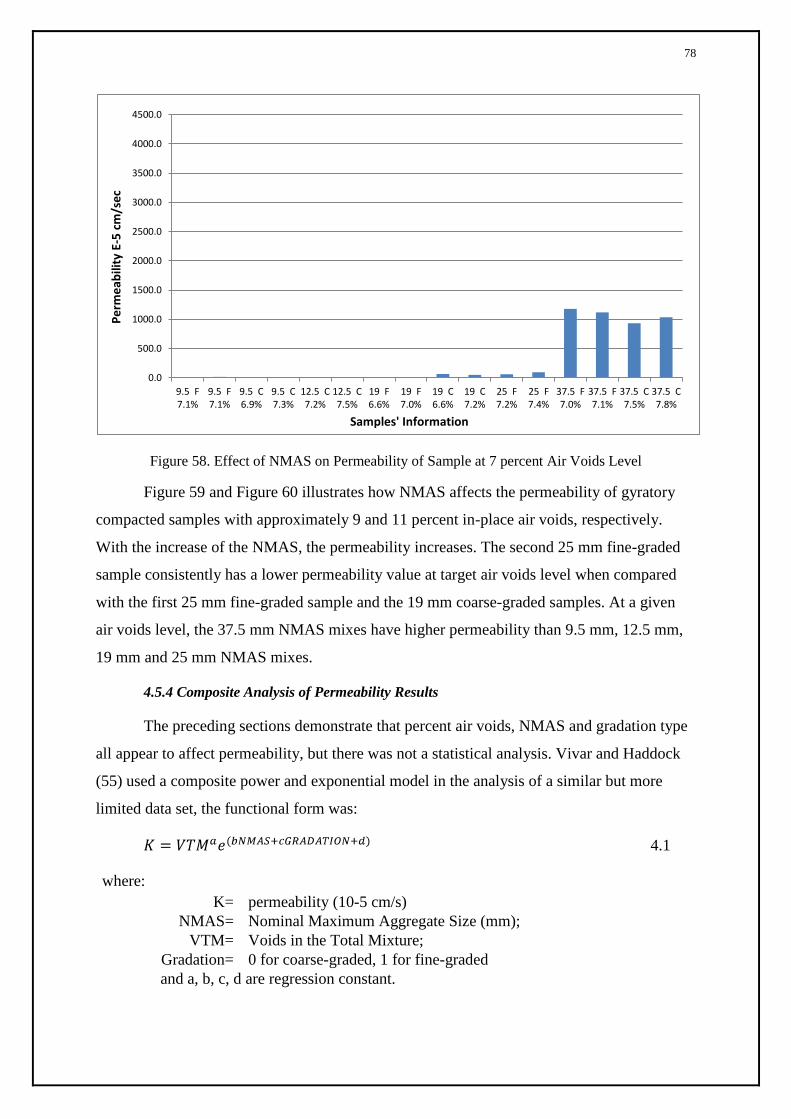
78
Figure 58. Effect of NMAS on Permeability of Sample at 7 percent Air Voids Level
Figure 59 and Figure 60 illustrates how NMAS affects the permeability of gyratory
compacted samples with approximately 9 and 11 percent in-place air voids, respectively.
With the increase of the NMAS, the permeability increases. The second 25 mm fine-graded
sample consistently has a lower permeability value at target air voids level when compared
with the first 25 mm fine-graded sample and the 19 mm coarse-graded samples. At a given
air voids level, the 37.5 mm NMAS mixes have higher permeability than 9.5 mm, 12.5 mm,
19 mm and 25 mm NMAS mixes.
4.5.4 Composite Analysis of Permeability Results
The preceding sections demonstrate that percent air voids, NMAS and gradation type
all appear to affect permeability, but there was not a statistical analysis. Vivar and Haddock
(55) used a composite power and exponential model in the analysis of a similar but more
limited data set, the functional form was:
4.1
where:
K= permeability (10-5 cm/s)
NMAS= Nominal Maximum Aggregate Size (mm);
VTM= Voids in the Total Mixture;
Gradation= 0 for coarse-graded, 1 for fine-graded
and a, b, c, d are regression constant.
0.0
500.0
1000.0
1500.0
2000.0
2500.0
3000.0
3500.0
4000.0
4500.0
9.5 F7.1%
9.5 F7.1%
9.5 C6.9%
9.5 C7.3%
12.5 C7.2%
12.5 C7.5%
19 F6.6%
19 F7.0%
19 C6.6%
19 C7.2%
25 F7.2%
25 F7.4%
37.5 F7.0%
37.5 F7.1%
37.5 C7.5%
37.5 C7.8%
Pe
rme
abili
ty E
-5 c
m/s
ec
Samples' Information

79
Through algebraic manipulation the equation can be transformed to:
4.2
The coefficients b, c, and d in equation 4.1 are divided by log (e) to compute b1, c1,
and d1. The transformed equation is then suitable for analysis using the multi-regression
function of Excel. The regression output using the Vivar functional model to fit the
WVUATL data are given in Table 23.
Figure 59. Effect of NMAS on Permeability of Sample at 9 percent Air Voids Level
0
500
1,000
1,500
2,000
2,500
3,000
3,500
4,000
4,500
9.5 F9.0%
9.5 F9.5%
9.5 C8.7%
9.5 C8.9%
12.5 C8.8%
12.5 C8.9%
19 F8.5%
19 F8.8%
19 C8.6%
19 C8.7%
25 F9.3%
25 F9.8%
37.5 F8.5%
37.5 F8.5%
37.5 C9.0%
37.5 C9.3%
Pe
rme
abili
ty E
-5 c
m/s
ec
Samples' Information

80
Figure 60. Effect of NMAS on Permeability of Sample at 11 percent Air Voids Level
The adjusted R2 indicates the equation explains most of the variation in the data. This
conclusion is supported by the finding of the F test showing the equation has statistical
significance at = 0.05. The significance of the coefficients is evaluated with the t-test; if the
P-value is greater than 0.05 the coefficient is considered to be statistically insignificant. In
this case, the c1 coefficient for GRADATION is statistically insignificant and should not be
included in the equation. The regression analysis was repeated without the c1 term producing
the results in Table 24.The adjusted R2 indicates the equation explains most of the variation
in the data. The F test demonstrates statistical significance of the equation and the t-test
shows both independent variables are significant at = 0.05. The P-value of the t-test
supports inclusion of the percent air voids and NMAS variables.
The coefficients from the regression analysis were transformed to match the
functional form of Equation 4.1. The three models are presented in Table 25:
Table 23. Power-exponential model of laboratory permeability data
0
500
1,000
1,500
2,000
2,500
3,000
3,500
4,000
4,500
9.5 F10.7%
9.5 F11.7%
9.5 C11.2%
9.5 C11.5%
12.5 C11.4%
12.5 C11.8%
19 F10.2%
19 F11.9%
19 C10.0%
19 C10.2%
25 F10.5%
25 F11.1%
37.5 F9.3%
37.5 F10.4%
37.5 C10.3%
37.5 C11%
Pe
rme
abili
ty E
-5 c
m/s
ec
Samples' Information

81
Regression Statistics Multiple R 0.946 R Square 0.894 Adjusted R
Square 0.889 Standard Error 0.428 Observations 64 ANOVA
df SS MS F
Significance
F
Regression 3 92.846 30.948 168.800 3.34E-29
Residual 60 11.000 0.1833 Total 63 103.847
Coefficients
Standard
Error t Stat P-value
d1 -5.09173 0.314 -16.205 1.38E-23
a 6.761749 0.330 20.450 8.71E-29
b1 0.050298 0.005 9.882 3.34E-14
c1 -0.07194 0.108 -0.665 0.508814
Table 24. Power-exponential model of laboratory permeability data without gradation variable
Regression Statistics Multiple R 0.945 R Square 0.893 Adjusted R
Square 0.890 Standard Error 0.426 Observations 64 ANOVA
df SS MS F Significance F
Regression 2 92.765 46.383 255.316 2.29E-30
Residual 61 11.082 0.182 Total 63 103.847
Coefficients
Standard
Error t Stat P-value d1 -5.12035 0.310 -16.527 3.33E-24
A 6.765393 0.328 20.608 3.58E-29 b1 0.049803 0.005 9.937 2.27E-14
Table 25. The results of the three models
Coefficient Vavir WVUATL Results
with GRADATION
WVUATL Results
without GRADATION
a 6.8 6.76 6.77
b 0.11 0.12 0.11

82
c -0.89 -0.17 NA
d -10.97 -11.72 -11.79
The various models are compared in Figure 61 for the 9.5 mm mix. The 9.5 mm mix
was selected for this comparison as it is the only mix type with sufficient field data for
modeling. The Vavir model with for the fine gradation compares very favorably with the
WVUATL model of the laboratory data. With respect to the effect of coarse versus fine
gradation, the Vivar model shows a major difference between the coarse and fine mixes.
This amount of difference did not exist in the WVUATL data set. The model developed from
the WVUATL data for only the 9.5 mm samples shows a greater effect of gradation type than
the general WVUATL model, but this difference is still much less than for the Vivar model.

83
Figure 61. Comparison of permeability models
0
100
200
300
400
500
600
700
0 2 4 6 8 10 12 14 16
Pe
rme
abili
ty E
-5 c
m/s
ec
Percent Air Voids
Field Data Model
9.5 mm Coarse WVUATL Model
Trend Line, Lab, 9.5 mm Fine
Trend, Lab, 9.5 mm Coarse
9.5 WVUATL Without Gradation
9.5 mm Fine Vivar Model
9.5 mm Coarse Vivar Model
9.5 mm Fine WVUATL Model

84
Finally the model developed for the field cores is included on Figure 61. The trend of
field cores having measureable permeability at low air voids and the model of the lab data
having a greater slope at high air voids is very similar to Cooley et al.’s (57) conclusion as
shown on Figure 22. While the trend found in the WVUATL data and Cooley’s results are
similar, the magnitude of the permeability in the Cooley study was higher. For example at
10 percent air voids the permeability of the Cooley and WVUATL results are approximately
400 x10-5
and 200x10-5
cm/sec, respectively. The difference in the permeability between the
Cooley and the WVUATL results may be explained by the fact that Cooley used 50 mm
samples and the WVUATL samples were 75 mm. Solaimanian (41) found for laboratory
compacted pills the permeability is influenced by sample height even though the height of the
sample is theoretically accounted for in Equation 2.8. Solaimanian did not present the data to
support this observation and did not identify if increasing height increases or decreased
permeability. By comparing laboratory permeability of compacted samples with different
thickness, Hanin et al (35) found an increase in thickness will results in a decrease in
permeability.

85
Chapter 5 Conclusions and Recommendations
5.1 Conclusions
The work performed in this research can be grouped into four topics:
Field permeability/ infiltration rates
Density and bulk specific gravity test methods on field cores
Permeability of field cores
Permeability of laboratory pills
5.1.1 Field permeability/ infiltration rates
The field permeability tests conducted on the 1.5 inch overlay project was not
successful, and potential reason can be: 1. the pavement surface was too hot, 2. the sealing
material was not reliable, and 3. the NCAT Permeameter cannot be applied for measuring the
field permeability of overlay projects. At the other three project sites, useful data were
collected, but in practice, it is difficult to determine the thickness of the pavement underneath
the NCAT Permeameter, so “infiltrate rate”, which estimates the flow rate of water penetrate
the pavement surface can be a better descriptor than permeability for the measurements made
with the NCAT Permeameter. While measurements were collected on at Chestnut Ridge, the
lack of measurements before the application of the fog seal eliminated the possibility of
evaluating the effectiveness of the treatment. On the Mon-Fayette Expressway and Quarry
Run Road, the measurements before and after the fog seal indicated a reduction in infiltration
rate. However there were too few data points for a meaningful statistical analysis.
5.1.2 Density and bulk specific gravity test methods on field cores
Although no statistically designed experiment was performed, data from a I 79 project
were evaluated which produced several interesting observations. The thin lift gauge had
smaller correction factors than the standard nuclear gauges. The correction factors for joint
locations were greater than mainline correction factors. Developing correction factors based
on the ration of the means may be better than using the difference of means methods. The
standard nuclear gauges and thin lift gauge did have strong correlation to laboratory Gmb
measurements.
Pair t test was conducted to identify if significant difference existed in Gmb data
collected by the contractor and WVUATL using T 166, and the computed p-value suggested

86
that null hypothesis that the two dataset are different, cannot be rejected. The line on equality
regression also indicates the results from the two labs are statistically similar.
The WVUATL CoreLok was used to evaluate a set of cores at the contractor’s lab.
These cores were reevaluated in the WVUATL. The pair t-test of the two sets of results
resulted in rejecting the null hypothesis. However, the variance of the test results was so
small that even a small difference in mean values would result in rejecting the null hypothesis,
indicating that the results of the t-test may not be reliable for this situation. The line on
equality regression also indicates the results from the two labs are statistically similar.
Gmb data from a contractor’s CoreLok and the corresponding cores from a project on
I 64 were provided to the WVUATL and tested with the CoreLok. Both the t-test and the line
of equality regression reject the statistical probability that the data from the two tests are
similar. This result is in conflict with the conclusions of Cooley et al. (6).
The comparison between Gmb data measured by T166 and CoreLok methods indicates
that CoreLok is a viable device for determining the Gmb and corresponding air voids of field
cores. Based upon the data collected, the CoreLok method did in general result in lower Gmb
values and thus higher air voids content than T166. The statistical analysis rejected the null
hypothesis for the entire data set. The current T 166 requires the use of the paraffin,
AASHTO T 2757, method when the water absorption is greater than two percent by volume.
The comparison of T 166 to the CoreLok method, AASHTO T 331, rejected the null
hypothesis of equal means when the absorption is greater than two percent. The null
hypothesis was not rejected when the percent absorption is less than two percent. This
analysis supports the current T 166 threshold. There is a proposed change to T166 to change
the threshold to one percent, and use T 331, the vacuum sealing method in lieu of T 275. The
t-test results indicate this is an acceptable policy as there was a significant difference in the
means of the two test methods for absorption greater than one percent, but at absorption
values less than one percent the null hypothesis was not rejected. The data collected in this
study shown that a threshold of one percent may be a conservative but it is accurate. From a
practical point of view, absorption is greater than one percent for many of the pills and cores.
Hence the contractors and WVDOH labs will need the vacuum seal equipment for measuring
Gmb. If the vacuum seal equipment is available it could, and probably should, be used for all
measurements of Gmb.
7 AASHTO T 275 is a difficult method and is being displaced by the vacuum seal method,
AASHTO T 331.
87
5.1.3 Permeability of field cores
The laboratory permeability results collected from field cores confirm that a strong
relationship exists between permeability and air voids content. At a low air voids content, the
permeability is typically low, and when the air voids content above certain point, a small
increase in air voids causes the correspondingly permeability value changes greatly. Cores
from longitudinal joints have higher in-place air voids than the mainline cores. In this study,
most of the cores from the longitudinal joints failed to meet the density requirement and
showed excessive permeability characteristics.
In general the permeability of the field cores on this project is consistent with the rule
of thumb that permeability becomes an issue when the air voids of the sample are greater than
eight percent. The regression model of the field cores permeability indicates that at eight
percent air voids the permeability is about 80x10-5 cm/sec which is less than the
recommended criteria of 100x10-5 cm/sec to 125x10-5 cm/sec.
5.1.4 Permeability of laboratory pills
The designed experiment to study the effects of mix type, gradation, and percent air
voids produced results similar to what is in the literature. As expected air voids has the
greatest effect on permeability. The mix type, as defined by the NMAS, was also a
significant effect. Contrary to the finding of some researchers gradation, classified as either
coarse or fine, was not a significant factor. There was a trend for coarse graded mixes to have
higher permeability than fine graded mixes, but the effect was not large enough to be
captured in the regression analysis. The laboratory permeability data were modeled using a
functional form developed by Vivar (55) and the regression coefficients for percent air voids
and NMAS were very similar with the exception of the gradation factor. The degree of
agreement between the Vivar model and the model developed from the WVUATL data was
unexpected as the inference space of Vivar’s model was limited to 9.5 mm and 19 mm mixes,
so it was an extrapolation to compare Vivar’s model to one developed from data for the full
range of available SuperPave mix types.
The comparison of the permeability of field cores to laboratory pills showed a similar
trend to the findings in the literature (57). Field cores have measureable permeability at
lower percent air voids than laboratory pills, but following the onset of permeability the slope
with respect to percent air voids of the laboratory pills is greater than the field cores.

88
5.2 Recommendations
Most of the field cores that been sent to the West Virginia University Asphalt
Technology Laboratory were from 9.5 mm NMAS mixes; only eight cores from 19 mm
NMAS were evaluated. The conclusions of this research would be enhanced if field cores for
the full range of mix types were evaluated.
Eight different HMA mixes were prepared for the density and laboratory permeability
measurements, with 37.5 mm coarse-graded mix simply prepared for purpose of permeability
measurements. To complete the understanding of how air voids content, aggregate gradation
and NMAS affect the permeability characteristics of HMA mixes, the 12.5 mm fine-graded,
25 mm coarse -graded and 37.5 mm coarse-graded HMA mixes should be designed and
prepared and tested for permeability.
The effect of gradation on permeability was not significant in this study. This may be
the result of the gradations being too similar to find capture this effect. The classification of
mix as either coarse or fine can be a difference of two percent of the material passing the
primary control sieve. The need for developing an alternative definition for coarse and fine
mixes for classifying the gradation with respect to permeability should be evaluated.
The laboratory permeability collected from the gyratory compacted pills shows that
the HMA samples tend to have low permeability value below approximately 6.5 percent air
voids content except the 37.5 mm fine-grade and coarse-graded HMA mixes. The 19 mm
NMAS and 25 mm NMAS HMA mixes seems to have lower permeability than the
information stated in literature review. One potential reason can be the thickness of gyratory
compacted samples. Presented in the Florida Method of Laboratory Permeability Test, the
thickness of the sample should be less than 80 mm which is the capability of the calibrated
cylinder. However, according to Virginia Test Method 120, “Method of Test for
Measurement of Permeability of Bituminous Paving Mixtures Using a Flexible Wall
Permeameter”, for 9.5 mm NMAS mixtures, the required height is 38±2 mm, for 19 mm
NMAS mixtures, the required height is 50±2 mm. So, samples should be prepared at different
thickness for the purpose of determining the permeability threshold of a HMA mixes.

89
References
1. Williams. R. C., Early Permeability test for Asphalt Mixture, Final Report R107-053.,
Missouri Department of Transportation, 2009.
2. Brown, E. R, D. Decker, R. B. Mallick, and J. Bukowski. Superpave Construction
Issues and Early Performance Evaluations. Journal of the Association of Asphalt
Paving Technologists, Volume 68, Chicago, Illinois, 1999.
3. Zube, E. Compaction Studies of Asphalt Concrete Pavements as Related to the Water
Permeability Test. Bulletin 358. Highway Research Board, National Research Council,
Washington, D.C., 1962.
4. Choubane, B, G.C. Page, and J.A. Musselman. Investigation of Water Permeability of
Coarse Graded Superpave Pavements. Journal of the Association of Asphalt Paving
Technologists, Volume 67,St. Paul, Minn., 1998.
5. Cooley, Jr., L.A., and E.R. Brown. Selection and Evaluation of a Field Permeability
Device for Asphalt Pavements. Transportation Research Board. No. 1723, Part 2:
Asphalt Mixtures 2000, Washington, D.C., 2000.
6. Cooley, Jr., L.A., Brain D. P., M.R. Hainin., M.S. Buchanan., and J. Harrington., Bulk
Specific Gravity Round-Robin Using the CoreLok Vacuum Sealing Device. NCAT
Report 02-11, 2002.
7. Kanitpong, K., C. H. Benson., and H. U. Bahia., Hydraulic Conductivity of Laboratory
Compacted Asphalt Mixtures. Transportation Research Record: Journal of the
Transportation Research Board, Volume 1767/2001, Page 25-32, Washington, D.C.,
2001.
8. Williams, S. G., Non-nuclear methods for HMA density measurements, MBTC 2075
Final Report, Arkansas, 2008.
9. Pratico, F. G., et al., Comparing Different of Procedures for the Measurement of the
Bulk Specific Gravity for Compacted HMA samples, 4th
International Siiv Congress-
Palermo (Italy), 2007.
10. Buchanan, M. S., An Evaluation of Selected Methods for Measuring the Bulk Specific
Gravity of Compacted Hot Mix Asphalt (HMA) Mixes. Association of Asphalt Paving
Technologist, Vol. 69, pp. 608–634, St. Paul, Minn., 2000.
11. Bhattacharjee, S., and Mallick, R. B., An Alternative Approach to Determination of
Bulk Specific Gravity and Permeability of Hot Mix Asphalt (HMA).International
Journal of Pavement Engineering, Volume 3, Page 143-152, Washington DC, 2002.
12. http://www.instrotek.com/pdfs/CoreLok_Manual.pdf, CoreLok Operator’s Guide,
accessed 6/17/2012.
13. Buchanan, M. S. and T. D. White., Hot Mix Asphalt Mix Design Evaluation Using
the CoreLok Vacuum-Sealing Device. Journal of Materials in Civil Engineering, ASCE,
Vol.17, No. 2, pp. 137-142, 2005.
14. Williams, Brett A., Williams, R. Christopher, and Bausano, Jason P, Criterion Test for
Method Selection in Determining the Bulk Specific Gravity of Hot Mix Asphalt,
Journal of ASTM International, Volume 4, Issue I, 2007.
15. Hall, K. D., F. T. Griffith, and S. G. Williams. Examination of Operator Variability
for Selected Methods for Measuring Bulk Specific Gravity of Hot Mix Asphalt

90
Concrete. In Transportation Research Record: Journal of the Transportation Research
Board, No. 1761, TRB, National Research Council, Washington, D.C., 2001, pp. 81-85.
16. Padlo, P. T., J. Mahoney, L. Aultman-Hall., and S. Zinke., Correlation of Nuclear
Density Readings with Cores Cut from Compacted Roadways, Connecticut Department
of Transportation, Report CT-2242-F-05-5, 2005.
17. Pavement Guide Interactive, http://www.pavementinteractive.org/article/nuclear-
density-gauge/,2010,accessed 6/17/2012.
18. Malpass, G., and N. P. Khosla., Evaluation of Gamma Ray Technology for the
Measurement of Bulk Specific Gravity of Compacted Asphalt Concrete Specimens,
Asphalt Paving Technology: Association of Asphalt Paving Technology-Proceedings of
the Technical Sessions 2002, page 352-367.
19. Mitchell, T.M., Density Monitoring on Asphalt pavement. Better Roads, Volume 54,
Issue Number 12, Page 22-25, 1984.
20. Zha, J., Revisions of California Testing Method 11 for Nuclear Gage Calibration.
2000, California Department of Transportation: Sacramento. P. 1-18.
21. Zha, J., Method of Developing Density and moisture calibration tables for the nuclear
gage, California Test 111, 2002.
22. Parker, F. and M.S. Hossain., An Analysis of Hot mix Asphalt mat density
measurement. Journal of Testing and Evaluation, ASTM, Vol.23, No. 6, pp415-423,
1995.
23. Smith, B. C.., and B. K. Diefenderfer., Comparison of Nuclear and Nonnuclear
Pavement Density Testing Devices. Transportation Research Record: Journal of the
Transportation Research Board, No. 2081, page 121-129, 2008.
24. Williams, S. G., Non-nuclear Methods for HMA Density Measurements, MBTC 2075
Final Report, Arkansas, 2008.
25. Romero, P. Laboratory Evaluation of the PQI Model 300. Project Report. Multiple
State Pooled Fund Study, DTFH61-00-P-00549, 2000.
26. NCHRP-IDEA, Pavement Quality Indicator, NCHRP Project 32 and 47,
Transportation Research Board, Washington, D.C., 1999.
27. Brown, G. O., “Henry Darcy and the making of a law”, Water Resources Research,
Vol. 38, No.7, 2002.
28. Maupin, Jr., G.W., Asphalt Permeability Testing Between Laboratories, Virginia
Transportation Research Council, Final Report, VTRC 05-R24, 2005.
29. Maupin, Jr., G.W., Examination of an Implemented Asphalt Permeability
Specification, Final Report VTRC 11-R7, 2010.
http://www.virginiadot.org/vtrc/main/online_reports/pdf/11-r7.pdf, accessed 6/17/2012
30. Hudson, S.B. and R.L. Davis. Relationship of Aggregate Voidage to Gradation.
Journal of the Association of Asphalt Paving Technologists, Volume 34. Page 574-593,
1965.
31. Choubane, B., G.C. Page, and J.A. Musselman. Investigation of Water Permeability
of Coarse Graded Superpave Pavements. Journal of the Association of Asphalt Paving
Technologists, Volume 67. 1998.

91
32. Cooley, L.A. Jr., E.R. Brown., and S. Maghsoodloo., Development of Critical Field
Permeability and Pavement Density Values for Coarse Graded Superpave Pavements.
NCAT Report 01-03, 2001.
33. Fwa, T.F., S.A. Tan., and Y.K. Guwe., Laboratory Evaluation of Clogging Potential
of Porous Asphalt Mix. Transportation Research Board of the National Academies,
Volume 1681/1999, Page 43-49, 2007.
34. Mallick, R.B., L. Allen Cooley, Jr., M.R. Teto., R.L. Bradbury., and D. Peabody., An
Evaluation of Factors Affecting Permeability of Superpave Designed Pavements,
NCAT Report 03-02, 2003.
35. Hainin, M.R., L.A. Cooley, Jr., and B.D. Prowell., An Investigation of Factors
Influencing Permeability of Superpave Mixes, International Journal of Pavements,
Volume 2, Page 41-52, 2003.
36. Ford, M.C., and C.E. McWilliams. Asphalt Mix Permeability. University of Arkansas,
Fayettville, AR, 1988.
37. Gogula, A. K., M. Hossain., and S. A. Romanoschi., A Study of Factors Affecting the
Permeability of Superpave Mixes in Kansas, Final Report No. K-TRAN: KUS-00-2,
KDOT, 2004.
38. Giompalo, J. A., Permeability of Hot Mix Asphalt Concrete as Affected by Binder
Content, Master Dissertation, West Virginia University, 2010.
39. Brown, E. R., M. R. Hainin., L.A. Cooley, Jr., and G. Hurley., Relationships of HMA
In-Place Air Voids, Lift Thickness, and Permeability, NCHRP Report 531,
Transportation Research Board of the National Academies, 2004.
40. Retzer, N., Permeability Research with the Romus Air Permeameter, Report No.
CDOT-2008-5, Final Report, Colorado Department of Transportation, 2008.
41. Solaimanian, M., Correlation of Laboratory-Compacted and Field-Compacted Hot-
Mix Asphalt Permeability, Final Report, Project No. 060704, Pennsylvania Department
of Transportation, 2010.
42. Maupin, G.W. Jr., Investigation of Test Methods, Pavement, and Laboratory Design
Related to Asphalt Permeability. Final Report, VTRC 00-R24, Virginia Transportation
Research Council, 2000.
43. Florida Method of Test for Measurement of Water Permeability of Compacted
Asphalt Paving Mixtures, Designation: FM 5-565, 2000, Revised 2006.
44. Cooley, L.A., Jr., “Permeability of Superpave Mixtures: Evaluation of Field
Permeameters”, NCAT, Report No. 99-1, National Center for Asphalt Technology,
February 1999.
45. Daniel, J.S., R.B. Mallick., and W.S. Mogawer., Evaluation of a Field Permeameter as
a Longitudinal Joint Quality Indicator, NETCR 64, Project No.03-5, New England
Transportation Consortium, 2007.
46. Williams, S.G., A. Pervis., L.S. Bhupathiraju., and A, Porter., Methods for Evaluating
Longitudinal Joint Quality in Asphalt Pavements, Transportation Research Board:
Journal of the Transportation Research Board, No.2098, Transportation Research Board
of the National Academies, Page 113-123, Washington, D.C., 2009.
47. Williams, S. G., A Comprehensive Study of Field Permeability Using the Vacuum
Permeameter, Project MBTC-2054, 2006.
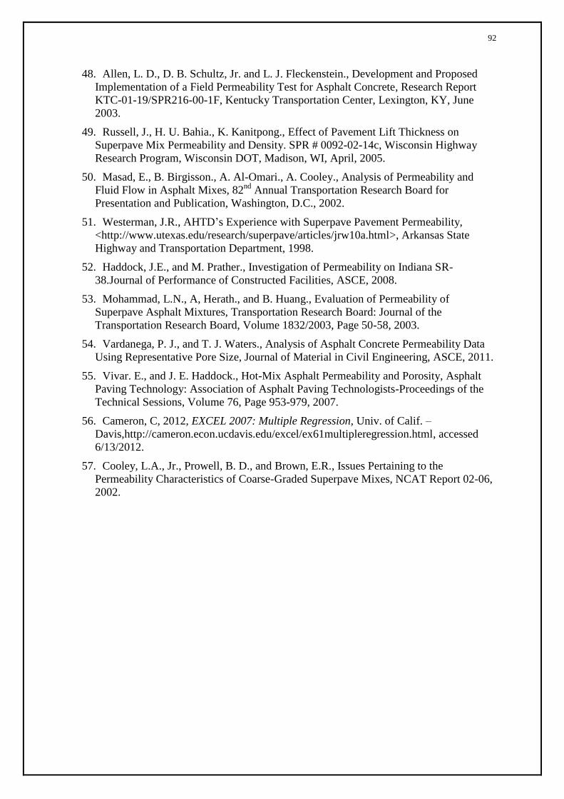
92
48. Allen, L. D., D. B. Schultz, Jr. and L. J. Fleckenstein., Development and Proposed
Implementation of a Field Permeability Test for Asphalt Concrete, Research Report
KTC-01-19/SPR216-00-1F, Kentucky Transportation Center, Lexington, KY, June
2003.
49. Russell, J., H. U. Bahia., K. Kanitpong., Effect of Pavement Lift Thickness on
Superpave Mix Permeability and Density. SPR # 0092-02-14c, Wisconsin Highway
Research Program, Wisconsin DOT, Madison, WI, April, 2005.
50. Masad, E., B. Birgisson., A. Al-Omari., A. Cooley., Analysis of Permeability and
Fluid Flow in Asphalt Mixes, 82nd
Annual Transportation Research Board for
Presentation and Publication, Washington, D.C., 2002.
51. Westerman, J.R., AHTD’s Experience with Superpave Pavement Permeability,
<http://www.utexas.edu/research/superpave/articles/jrw10a.html>, Arkansas State
Highway and Transportation Department, 1998.
52. Haddock, J.E., and M. Prather., Investigation of Permeability on Indiana SR-
38.Journal of Performance of Constructed Facilities, ASCE, 2008.
53. Mohammad, L.N., A, Herath., and B. Huang., Evaluation of Permeability of
Superpave Asphalt Mixtures, Transportation Research Board: Journal of the
Transportation Research Board, Volume 1832/2003, Page 50-58, 2003.
54. Vardanega, P. J., and T. J. Waters., Analysis of Asphalt Concrete Permeability Data
Using Representative Pore Size, Journal of Material in Civil Engineering, ASCE, 2011.
55. Vivar. E., and J. E. Haddock., Hot-Mix Asphalt Permeability and Porosity, Asphalt
Paving Technology: Association of Asphalt Paving Technologists-Proceedings of the
Technical Sessions, Volume 76, Page 953-979, 2007.
56. Cameron, C, 2012, EXCEL 2007: Multiple Regression, Univ. of Calif. –
Davis,http://cameron.econ.ucdavis.edu/excel/ex61multipleregression.html, accessed
6/13/2012.
57. Cooley, L.A., Jr., Prowell, B. D., and Brown, E.R., Issues Pertaining to the
Permeability Characteristics of Coarse-Graded Superpave Mixes, NCAT Report 02-06,
2002.

93
Appendix 1 Stockpile Gradation, Blend Gradation and Gradation Curve for Mixes
Table 26. 9.5 mm NMAS Fine Gradation
Bin #1 Bin #2 Bin #3 Bin #4
Elkins SKID 8's Elkins 9's Elkins SAND Baghouse Fine
% Used: 26 % Used: 15 % Used: 58 % Used: 1 Comb.
Gradation
Control
Points Sieve Size Passing % Total Passing % Total Passing % Total Passing % Total
2"(50 mm) 100.00 26.00 100.00 15.00 100.00 58.00 100.00 1.00 100.00
1.5"(37.5 mm) 100.00 26.00 100.00 15.00 100.00 58.00 100.00 1.00 100.00
1"(25 mm) 100.00 26.00 100.00 15.00 100.00 58.00 100.00 1.00 100.00
3/4"(19 mm) 100.00 26.00 100.00 15.00 100.00 58.00 100.00 1.00 100.00
1/2"(12.5 mm) 100.00 26.00 100.00 15.00 100.00 58.00 100.00 1.00 100.00 100
3/8" (9.5 mm) 93.40 24.30 100.00 15.00 100.00 58.00 100.00 1.00 98.30 90-100
#4 (4.75 mm) 7.90 2.10 76.00 11.40 99.90 57.90 100.00 1.00 72.40 90
#8 (2.36 mm) 2.10 0.60 8.20 1.20 82.40 47.80 100.00 1.00 50.60 32-67
#16 (1.18 mm) 1.90 0.50 3.50 0.50 51.20 29.70 100.00 1.00 31.70
#30 (600μm ) 1.80 0.50 2.90 0.40 32.00 18.60 99.90 1.00 20.50
#50 (300 μm) 1.70 0.40 2.60 0.40 19.80 11.50 99.70 1.00 13.30
#100 (150 μm) 1.60 0.40 2.50 0.40 12.30 7.10 95.40 1.00 8.90
#200 (75 μm) 1.40 0.40 2.20 0.30 8.00 4.60 70.10 0.70 6.00 2-10
Figure 62. Combined Gradation Charts for NMAS 9.5 mm Fine Superpave Mixes
Table 27. 9.5 mm NMAS Coarse Gradation
12
.5
9.5
4.7
5
2.3
6
0.0
75
0.1
5
0.3
0.6
1.1
8
0
5
10
15
20
25
30
35
40
45
50
55
60
65
70
75
80
85
90
95
100
Maximum DensityLine9.5 mm Coarse
Sieve Size (Raised to 0.45 Power), mm
Per
cen
t P
assi
ng
(%)

94
Bin #1 Bin #2 Bin #3 Bin #4
Elkins SKID 8's Elkins 9's Elkins SAND Baghouse Fine
% Used: 37 % Used: 25 % Used: 37 % Used: 1 Comb.
Gradation
Control
Points Sieve Size Passing % Total Passing % Total Passing % Total Passing % Total
2"(50 mm) 100.00 37.00 100.00 25.00 100.00 37.00 100.00 1.00 100.00
1.5"(37.5 mm) 100.00 37.00 100.00 25.00 100.00 37.00 100.00 1.00 100.00
1"(25 mm) 100.00 37.00 100.00 25.00 100.00 37.00 100.00 1.00 100.00
3/4"(19 mm) 100.00 37.00 100.00 25.00 100.00 37.00 100.00 1.00 100.00
1/2"(12.5 mm) 100.00 37.00 100.00 25.00 100.00 37.00 100.00 1.00 100.00 100
3/8" (9.5 mm) 93.40 34.55 100.00 25.00 100.00 37.00 100.00 1.00 97.55 90-100
#4 (4.75 mm) 7.90 2.91 76.00 19.00 99.90 36.96 100.00 1.00 59.87 90
#8 (2.36 mm) 2.10 0.79 8.20 2.05 82.40 30.49 100.00 1.00 34.33 32-67
#16 (1.18 mm) 1.90 0.70 3.50 0.88 51.20 18.94 100.00 1.00 21.52
#30 (600μm ) 1.80 0.67 2.90 0.73 32.00 11.84 99.90 1.00 14.23
#50 (300 μm) 1.70 0.64 2.60 0.65 19.80 7.33 99.70 1.00 9.62
#100 (150 μm) 1.60 0.59 2.50 0.63 12.30 4.55 95.40 0.95 6.72
#200 (75 μm) 1.40 0.52 2.20 0.56 8.00 2.96 70.10 0.70 4.74 2-10
Figure 63. Combined Gradation Charts for NMAS 9.5 mm Coarse Superpave Mixes
12
.5
9.5
4.7
5
2.3
6
0.0
75
0.1
5
0.3
0.6
1.1
8
0
5
10
15
20
25
30
35
40
45
50
55
60
65
70
75
80
85
90
95
100
Maximum Density Line
9.5 mm Coarse
Control Points
Sieve Size (Raised to 0.45 Power), mm
Per
cen
t P
assi
ng
(%)

95
Table 28. 12.5 mm NMAS Coarse Gradation
Bin #1 Bin #2 Bin #3 Bin #4 Bin #5
Elkins SKID 78’s Elkins Skid 8’s Elkins 9’s Elkins SAND Baghoues Fine
% Used: 15 % Used: 41 % Used: 13 % Used: 30 % Used: 1 Comb.
Gradation Control Points Sieve Size Passing % Total Passing % Total Passing % Total Passing
%
Total Passing %Total
2"(50 mm) 100.00 15.00 100.00 41.00 100.00 13.00 100.00 30.00 100.00 1.00 100.00
1.5"(37.5 mm) 100.00 15.00 100.00 41.00 100.00 13.00 100.00 30.00 100.00 1.00 100.00
1"(25 mm) 100.00 15.00 100.00 41.00 100.00 13.00 100.00 30.00 100.00 1.00 100.00
3/4"(19 mm) 100.00 15.00 100.00 41.00 100.00 13.00 100.00 30.00 100.00 1.00 100.00 100
1/2"(12.5 mm) 87.20 13.08 100.00 41.00 100.00 13.00 100.00 30.00 100.00 1.00 98.08 90-100
3/8" (2.36
mm) 36.90 5.54 93.40 38.29 100.00 13.00 100.00 30.00 100.00 1.00 87.83 90
#4 (4.75 mm) 6.10 0.92 7.90 3.24 76.00 9.88 99.90 29.97 100.00 1.00 45.00
#8 (2.36 mm) 4.00 0.60 2.10 0.86 8.20 1.07 82.40 24.72 100.00 1.00 28.25 28-58
#16 (1.18 mm) 3.50 0.53 1.90 0.78 3.50 0.46 51.20 15.36 100.00 1.00 18.12
#30 (600μm ) 3.40 0.51 1.80 0.74 2.90 0.38 32.00 9.60 99.90 1.00 12.22
#50 (300 μm) 3.30 0.50 1.70 0.70 2.60 0.34 19.80 5.94 99.70 1.00 8.47
#100 (150 μm) 2.80 0.42 1.60 0.66 2.50 0.33 12.30 3.69 95.40 0.95 6.05
#200 (75 μm) 2.60 0.39 1.40 0.57 2.20 0.29 8.00 2.40 70.10 0.70 4.35 2-10
Figure 64. Combined Gradation Charts for NMAS 12.5 mm Coarse Superpave Mixes
19
12
.5
9.5
4.7
5
2.3
6
0.0
75
0.1
5
0.3
0.6
1.1
8
0
5
10
15
20
25
30
35
40
45
50
55
60
65
70
75
80
85
90
95
100
Control PointsMaximum Density Line12.5 mm Coarse
Sieve Size (Raised to 0.45 Power), mm
Per
cen
t P
assi
ng
(%)

96
Table 29. 19 mm NMAS Fine Gradation
Bin #1 Bin #2 Bin #3 Bin #4 Bin #5
MG 67's Elkins 8’s Elkins 9’s Elkins SAND Baghoues Fine
% Used: 33 % Used: 20 % Used: 14 % Used: 32 % Used: 1 Comb.
Gradation
Control
Points Sieve Size Passing % Total Passing % Total Passing % Total Passing % Total Passing %Total
2"(50 mm) 100.00 33.00 100.00 20.00 100.00 14.00 100.00 32.00 100.00 1.00 100.00
1.5"(37.5 mm) 100.00 33.00 100.00 20.00 100.00 14.00 100.00 32.00 100.00 1.00 100.00
1"(25 mm) 100.00 33.00 100.00 20.00 100.00 14.00 100.00 32.00 100.00 1.00 100.00 100
3/4"(19 mm) 100.00 33.00 100.00 20.00 100.00 14.00 100.00 32.00 100.00 1.00 100.00 90-100
1/2"(12.5 mm) 61.00 20.13 100.00 20.00 100.00 14.00 100.00 32.00 100.00 1.00 87.13 90
3/8" (2.36 mm) 26.00 8.58 93.00 18.60 100.00 14.00 100.00 32.00 100.00 1.00 74.18
#4 (4.75 mm) 5.00 1.65 6.00 1.20 77.00 10.78 100.00 32.00 100.00 1.00 46.63
#8 (2.36 mm) 2.30 0.76 1.40 0.28 4.00 0.56 79.00 25.28 100.00 1.00 27.88 23-49
#16 (1.18 mm) 2.20 0.73 1.30 0.26 2.30 0.32 51.00 16.32 100.00 1.00 18.63
#30 (600μm ) 2.10 0.69 1.20 0.24 2.10 0.29 34.00 10.88 99.90 1.00 13.11
#50 (300 μm) 2.00 0.66 1.10 0.22 1.90 0.27 22.00 7.04 99.70 1.00 9.18
#100 (150 μm) 1.90 0.63 1.00 0.20 1.70 0.24 12.00 3.84 95.40 0.95 5.86
#200 (75 μm) 1.40 0.46 0.80 0.16 1.20 0.17 7.20 2.30 70.10 0.70 3.80 2-8
97
Figure 65. Combined Gradation Charts for NMAS 19 mm Fine Superpave Mixes
Table 30. 19 mm NMAS Coarse Gradation
Bin #1 Bin #2 Bin #3 Bin #4
MG 67's Elkins 8’s Elkins 9’s Elkins SAND
% Used: 43 % Used: 14 % Used: 7 % Used: 36 Comb. Gradation
Control Points
Sieve Size Passing % Total Passing % Total Passing % Total Passing % Total
2"(50 mm) 100.00 43.00 100.00 14.00 100.00 7.00 100.00 36.00 100.00
1.5"(37.5 mm) 100.00 43.00 100.00 14.00 100.00 7.00 100.00 36.00 100.00
1"(25 mm) 100.00 43.00 100.00 14.00 100.00 7.00 100.00 36.00 100.00 100
3/4"(19 mm) 100.00 43.00 100.00 14.00 100.00 7.00 100.00 36.00 100.00 90-100
1/2"(12.5 mm) 61.00 26.23 100.00 14.00 100.00 7.00 100.00 36.00 83.23
3/8" (2.36 mm) 26.00 11.18 93.00 13.02 100.00 7.00 100.00 36.00 67.20 23-49
#4 (4.75 mm) 5.00 2.15 6.00 0.84 77.00 5.39 100.00 36.00 44.38
#8 (2.36 mm) 2.30 0.99 1.40 0.20 4.00 0.28 79.00 28.44 29.91
#16 (1.18 mm) 2.20 0.95 1.30 0.18 2.30 0.16 51.00 18.36 19.65
#30 (600μm ) 2.10 0.90 1.20 0.17 2.10 0.15 34.00 12.24 13.46
#50 (300 μm) 2.00 0.86 1.10 0.15 1.90 0.13 22.00 7.92 9.07
#100 (150 μm) 1.90 0.82 1.00 0.14 1.70 0.12 12.00 4.32 5.40
#200 (75 μm) 1.40 0.60 0.80 0.11 1.20 0.08 7.20 2.59 3.39 2-8
25
19
12
.5
9.5
4.7
5
2.3
6
0.0
75
0
.15
0.3
0.6
1.1
8
0
5
10
15
20
25
30
35
40
45
50
55
60
65
70
75
80
85
90
95
100
Control Points
Maximum Density Line
19 Fine
Sieve Size (Raised to 0.45 Power), mm
Per
cen
t P
assi
ng
(%)

98
Figure 66. Combined Gradation Charts for NMAS 19 mm Coarse Superpave Mixes
Table 31. 25 mm NMAS Fine Gradation
Bin #1 Bin #2 Bin #3 Bin #4
Elkins 57's Elkins 8’s Elkins 9’s MG SAND
% Used: 43 % Used: 14 % Used: 7 % Used: 36 Comb. Gradation
Control Points
Sieve Size Passing % Total Passing % Total Passing % Total Passing % Total
2"(50 mm) 100.00 43.00 100.00 14.00 100.00 7.00 100.00 36.00 100.00
1.5"(37.5 mm) 100.00 43.00 100.00 14.00 100.00 7.00 100.00 36.00 100.00 100
1"(25 mm) 92.00 39.56 100.00 14.00 100.00 7.00 100.00 36.00 96.56 90-100
3/4"(19 mm) 69.00 29.67 100.00 14.00 100.00 7.00 100.00 36.00 86.67 90
1/2"(12.5 mm) 29.00 12.47 100.00 14.00 100.00 7.00 100.00 36.00 69.47
3/8" (9.5 mm) 10.00 4.30 93.00 13.02 100.00 7.00 100.00 36.00 60.32
#4 (4.75 mm) 1.70 0.73 6.00 0.84 77.00 5.39 100.00 36.00 42.96
#8 (2.36 mm) 1.60 0.69 1.40 0.20 4.00 0.28 78.00 28.08 29.24 19-45
#16 (1.18 mm) 1.50 0.65 1.30 0.18 2.30 0.16 48.00 17.28 18.27
#30 (600μm ) 1.40 0.60 1.20 0.17 2.10 0.15 28.00 10.08 11.00
#50 (300 μm) 1.30 0.56 1.10 0.15 1.90 0.13 17.00 6.12 6.97
#100 (150 μm) 1.20 0.52 1.00 0.14 1.70 0.12 11.00 3.96 4.74
#200 (75 μm) 1.12 0.48 0.80 0.11 1.20 0.08 8.20 2.95 3.63 2-7
25
19
12
.5
9.5
4.7
5
2.3
6
0.0
75
0
.15
0.3
0.6
1.1
8
0
5
10
15
20
25
30
35
40
45
50
55
60
65
70
75
80
85
90
95
100
Control Points
Maximum Density Line
19 Coarse
Sieve Size (Raised to 0.45 Power), mm
Per
cen
t P
assi
ng
(%)

99
Figure 67. Combined Gradation Charts for NMAS 25 mm Fine Superpave Mixes
Table 32. 37.5 mm NMAS Fine Gradation
Bin #1 Bin #2 Bin #3 Bin #4 Bin #5
Elkins 4's MG 67’s MG 8’s Elk SAND BHF
% Used: 29 % Used: 29 % Used: 20 % Used: 21 % Used: 1 Comb. Gradation
Control Points Sieve Size Passing % Total Passing % Total Passing % Total Passing % Total Passing %Total
2"(50 mm) 100.00 29.00 100.00 29.00 100.00 20.00 100.00 21.00 100.00 1.00 100.00
1.5"(37.5 mm) 100.00 29.00 100.00 29.00 100.00 20.00 100.00 21.00 100.00 1.00 100.00 100
1"(25 mm) 45.70 13.25 100.00 29.00 100.00 20.00 100.00 21.00 100.00 1.00 84.25 90-100
3/4"(19 mm) 4.40 1.28 100.00 29.00 100.00 20.00 100.00 21.00 100.00 1.00 72.28 90
1/2"(12.5 mm) 1.30 0.38 40.80 11.83 100.00 20.00 100.00 21.00 100.00 1.00 54.21
3/8" (9.5 mm) 1.20 0.35 9.50 2.76 97.40 19.48 100.00 21.00 100.00 1.00 44.58
#4 (4.75 mm) 1.10 0.32 2.00 0.58 23.70 4.74 100.00 21.00 100.00 1.00 27.64
#8 (2.36 mm) 1.08 0.31 1.60 0.46 3.30 0.66 82.40 17.30 100.00 1.00 19.74 27-39
#16 (1.18 mm) 1.07 0.31 1.50 0.44 2.80 0.56 51.20 10.75 100.00 1.00 13.06
#30 (600μm ) 1.06 0.31 1.40 0.41 2.40 0.48 32.00 6.72 99.90 1.00 8.91
#50 (300 μm) 1.05 0.30 1.30 0.38 2.30 0.46 19.80 4.16 99.70 1.00 6.30
#100 (150 μm) 1.04 0.30 1.20 0.35 1.90 0.38 12.30 2.58 95.40 0.95 4.57
#200 (75 μm) 0.84 0.24 1.03 0.30 1.83 0.37 8.00 1.68 70.10 0.70 3.29 0-6
37
.5
25
19
12
.5
9.5
4.7
5
2.3
6
0.0
75
0
.15
0
.3
0.6
1.1
8
0
5
10
15
20
25
30
35
40
45
50
55
60
65
70
75
80
85
90
95
100
Control Points
Maximum Density Line
25 mm Fine
Sieve Size (Raised to 0.45 Power), mm
Per
cen
t P
assi
ng
(%)

100
Figure 68. Combined Gradation Charts for NMAS 37.5 mm Fine Superpave Mixes
Table 33. 37.5 mm NMAS Coarse Gradation
Bin #1 Bin #2 Bin #3 Bin #4 Bin #5
Elkins 4's MG 67’s MG 8’s Elk SAND BHF
% Used: 25 % Used: 27 % Used: 23 % Used: 24 % Used: 1 Comb. Gradation
Control Points
Sieve Size Passing % Total Passing % Total Passing % Total Passing % Total Passing %Total
2"(50 mm) 100.00 25.00 100.00 27.00 100.00 23.00 100.00 24.00 100.00 1.00 100.00
1.5"(37.5 mm) 100.00 25.00 100.00 27.00 100.00 23.00 100.00 24.00 100.00 1.00 100.00 100
1"(25 mm) 45.70 11.43 100.00 27.00 100.00 23.00 100.00 24.00 100.00 1.00 86.43 90-100
3/4"(19 mm) 4.40 1.10 100.00 27.00 100.00 23.00 100.00 24.00 100.00 1.00 76.10 90
1/2"(12.5 mm) 1.30 0.33 40.80 11.02 100.00 23.00 100.00 24.00 100.00 1.00 59.34
3/8" (9.5 mm) 1.20 0.30 9.50 2.57 97.40 22.40 100.00 24.00 100.00 1.00 50.27
#4 (4.75 mm) 1.10 0.28 2.00 0.54 23.70 5.45 100.00 24.00 100.00 1.00 31.27
#8 (2.36 mm) 1.08 0.27 1.60 0.43 3.30 0.76 82.40 19.78 100.00 1.00 22.24 15-41
#16 (1.18 mm) 1.07 0.27 1.50 0.41 2.80 0.64 51.20 12.29 100.00 1.00 14.60
#30 (600μm ) 1.06 0.27 1.40 0.38 2.40 0.55 32.00 7.68 99.90 1.00 9.87
#50 (300 μm) 1.05 0.26 1.30 0.35 2.30 0.53 19.80 4.75 99.70 1.00 6.89
#100 (150 μm) 1.04 0.26 1.20 0.32 1.90 0.44 12.30 2.95 95.40 0.95 4.93
#200 (75 μm) 0.84 0.21 1.03 0.28 1.83 0.42 8.00 1.92 70.10 0.70 3.53 0-6
50
37
.5
25
19
12
.5
9.5
4.7
5
2.3
6
0.0
75
0
.15
0
.3
0.6
1.1
8
0
5
10
15
20
25
30
35
40
45
50
55
60
65
70
75
80
85
90
95
100
Control Points
Maximum Density Line
37.5 mm Fine
Sieve Size (Raised to 0.45 Power), mm
Per
cen
t P
assi
ng
(%)
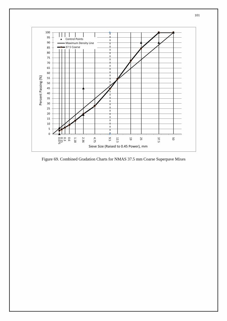
101
Figure 69. Combined Gradation Charts for NMAS 37.5 mm Coarse Superpave Mixes
50
37
.5
25
19
12
.5
9.5
4.7
5
2.3
6
0.0
75
0
.15
0
.3
0.6
1.1
8
0
5
10
15
20
25
30
35
40
45
50
55
60
65
70
75
80
85
90
95
100
Control Points
Maximum Density Line
37.5 Coarse
Sieve Size (Raised to 0.45 Power), mm
Per
cen
t P
assi
ng
(%)

102
Appendix 2 Field Density Data and Bulk Specific Gravity of Field Cores
WVUATL
Number Project Project
Mixes
Type (mm)
Lab Number Location M/J Gmm
Contractor
1 IM-0792(142)D/XC2187T I-79 9.5 JFA-A49-M 4190+19/9'SBSL M 2.461
2 IM-0792(142)D/XC2187T I-79 9.5 DOH-A49-M 4196+79/7'SBSL M 2.461
3 IM-0792(142)D/XC2187T I-79 9.5 JFA-A49-J 4190+19/4''SBSL J 2.461
4 IM-0792(142)D/XC2187T I-79 9.5 DOH-A49-J 4196+79/4''SBSL J 2.461
5 IM-0792(142)D/XC2187T I-79 9.5 JFA-A57-M 4113+01/5'SBSL M 2.461
6 IM-0792(142)D/XC2187T I-79 9.5 DOH-A57-M 4116+55/2'SBSL M 2.461
7 IM-0792(142)D/XC2187T I-79 9.5 JFA-A57-J 4113+01/4''SBSL J 2.461
8 IM-0792(142)D/XC2187T I-79 9.5 DOH-A57-J 4116+55/4''SBSL J 2.461
9 IM-0792(142)D/XC2187T I-79 9.5 JFA-A65-M 4037+50/10'SBSL M 2.461
10 IM-0792(142)D/XC2187T I-79 9.5 DOH-A65-M 4032+87/4'SBSL M 2.461
11 IM-0792(142)D/XC2187T I-79 9.5 JFA-A65-J 4037+50/4''SBSL J 2.461
12 IM-0792(142)D/XC2187T I-79 9.5 DOH-A65-J 4032+87/4''SBSL J 2.461
13 IM-0792(142)D/XC2187T I-79 9.5 JFA-A71-M 4035+81/5'NBSL M 2.461
14 IM-0792(142)D/XC2187T I-79 9.5 DOH-A71-M 4033+42/6'NBSL M 2.461
15 IM-0792(142)D/XC2187T I-79 9.5 JFA-A71-J 4035+81/4''NBSL J 2.461
16 IM-0792(142)D/XC2187T I-79 9.5 DOH-A71-J 4033+42/4''NBSL J 2.461
17 IM-0792(142)D/XC2187T I-79 9.5 4222+95 / 3' 4222+95/3' M 2.462
18 IM-0792(142)D/XC2187T I-79 9.5 4222+36 / 7' 4222+36/7' M 2.462
19 IM-0792(142)D/XC2187T I-79 9.5 4222+00 / 4' 4222+00/4' M 2.462
20 IM-0792(142)D/XC2187T I-79 9.5 4221+53 / 2' 4221+53/2' M 2.462
21 IM-0792(142)D/XC2187T I-79 9.5 4221+17 / 1' 4221+17/1' M 2.462
22 IM-0792(142)D/XC2187T I-79 9.5 4220+84 / 6' 4220+84/6' M 2.462
23 IM-0792(142)D/XC2187T I-79 9.5 4220+67 / 6' 4220+67/6' M 2.462
24 IM-0792(142)D/XC2187T I-79 9.5 4220+33 / 10' 4220+33/10' M 2.462
25 IM-0793(210)D/XC2186T I-79 9.5 - 9+51 / 12' (-)9+51/12' M 2.463
26 IM-0793(210)D/XC2186T I-79 9.5 - 9+15 / 11' (-)9+51/11' M 2.463
27 IM-0793(210)D/XC2186T I-79 9.5 - 8+52 / 6' (-)8+52/6' M 2.463
28 IM-0793(210)D/XC2186T I-79 9.5 - 8+23 / 10' (-)8+23/10' M 2.463
29 IM-0793(210)D/XC2186T I-79 9.5 - 7+76 / 10' (-)7+76/10' M 2.463
30 IM-0793(210)D/XC2186T I-79 9.5 - 7+56 / 6' (-)7+56/6' M 2.463
31 IM-0793(210)D/XC2186T I-79 9.5 - 6+53 / 8' (-)6+53/8' M 2.463

103
WVUATL
Number Project Project
Mixes Type
(mm)
Lab number Location M/L Gmm Contractor
32 IM-0793(210)D/XC2186T I-79 9.5 A23M-B 10+00 NBML/7' M 2.456
33 IM-0793(210)D/XC2186T I-79 9.5 A44M-A 6+00 NBSL/9' M 2.456
34 IM-0793(210)D/XC2186T I-79 9.5 A44M-B 10+00 NBSL/4'' M 2.456
35 IM-0793(210)D/XC2186T I-79 9.5 JFA-A103-M 161+32 SBML/4' M 2.456
36 IM-0793(210)D/XC2186T I-79 9.5 DOH-A103-M 165+53 SBML/4' M 2.456
37 IM-0793(210)D/XC2186T I-79 9.5 DOH-A104-M 178+56 SBML/3' M 2.456
38 IM-0793(210)D/XC2186T I-79 9.5 JFA-A104-M 171+56 SBML/6' M 2.456
39 IM-0793(210)D/XC2186T I-79 9.5 A23J-B 10+00 NBML/4'' J 2.456
40 IM-0793(210)D/XC2186T I-79 9.5 A23J-A 6+00 NBML/4'' J 2.456
41 IM-0793(210)D/XC2186T I-79 9.5 A44J-A 6+00 NBSL/4'' J 2.456
42 IM-0793(210)D/XC2186T I-79 9.5 A44J-B 10+00 NBML/4'' J 2.456
43 IM-0793(210)D/XC2186T I-79 9.5 DOH-A103-J 165+53 SBML/4'' J 2.456
44 IM-0793(210)D/XC2186T I-79 9.5 DOH-A104-J 178+56 SBML/4'' J 2.456
45 IM-0793(210)D/XC2186T I-79 9.5 JFA-104-J 171+56 SBML/4'' J 2.456
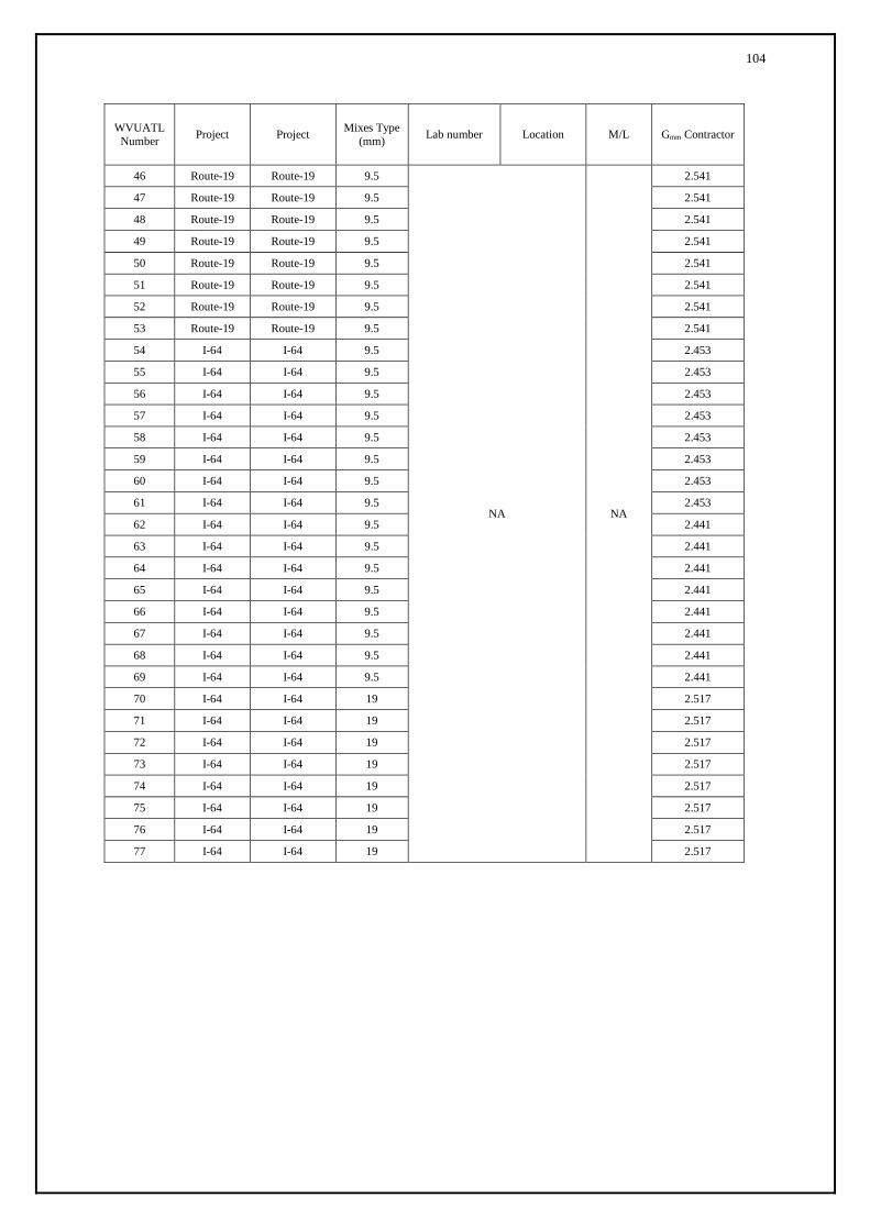
104
WVUATL
Number Project Project
Mixes Type
(mm) Lab number Location M/L Gmm Contractor
46 Route-19 Route-19 9.5
NA NA
2.541
47 Route-19 Route-19 9.5 2.541
48 Route-19 Route-19 9.5 2.541
49 Route-19 Route-19 9.5 2.541
50 Route-19 Route-19 9.5 2.541
51 Route-19 Route-19 9.5 2.541
52 Route-19 Route-19 9.5 2.541
53 Route-19 Route-19 9.5 2.541
54 I-64 I-64 9.5 2.453
55 I-64 I-64 9.5 2.453
56 I-64 I-64 9.5 2.453
57 I-64 I-64 9.5 2.453
58 I-64 I-64 9.5 2.453
59 I-64 I-64 9.5 2.453
60 I-64 I-64 9.5 2.453
61 I-64 I-64 9.5 2.453
62 I-64 I-64 9.5 2.441
63 I-64 I-64 9.5 2.441
64 I-64 I-64 9.5 2.441
65 I-64 I-64 9.5 2.441
66 I-64 I-64 9.5 2.441
67 I-64 I-64 9.5 2.441
68 I-64 I-64 9.5 2.441
69 I-64 I-64 9.5 2.441
70 I-64 I-64 19 2.517
71 I-64 I-64 19 2.517
72 I-64 I-64 19 2.517
73 I-64 I-64 19 2.517
74 I-64 I-64 19 2.517
75 I-64 I-64 19 2.517
76 I-64 I-64 19 2.517
77 I-64 I-64 19 2.517

105
WVUATL
Number
Gmb (Contractor
CoreLok)
Gmb (WVUATL CoreLok Performed
at Contractor Lab)
Gmb (WVUATL
CoreLok)
Gmb (Contractor
T166)
Gmb (WVDOH
T166)
Gmb (WVUATL
T166)
Water
Absorption
1
NA NA
2.218 2.241
2.236 1.4
2 2.302
2.320 2.311 0.4
3 2.210 2.218
2.230 1.5
4 2.184
2.206 2.197 3.0
5 2.280 2.292
2.290 0.4
6 2.269
2.288 2.282 0.7
7 2.207 2.218
2.220 1.3
8 2.165
2.198 2.188 3.4
9 2.173 2.201
2.200 2.4
10 2.345
2.353 2.353 0.4
11 2.174 2.209
2.209 2.3
12 2.152
2.187 2.181 3.5
13 2.302 2.318
2.313 0.4
14 2.293
2.311 2.307 0.7
15 2.146 2.163
2.159 3.3
16 2.213
2.230 2.233 2.0
17 2.277 2.302
2.286 0.6
18 2.234 2.258
2.240 1.0
19 2.271 2.298
2.280 0.7
20 2.199 2.232
2.221 1.1
21 2.159 2.194
2.162 1.7
22 2.210 2.228
2.218 1.1
23 2.258 2.272
2.264 0.7
24 2.267 2.280
2.281 0.7
25 2.163 2.176
2.164 3.4
26 2.170 2.176
2.173 3.1
27 2.216 2.223
2.217 2.4
28 2.044 2.050
2.048 7.9
29 2.102 2.107
2.109 3.6
30 2.199 2.201
2.204 1.8
31 2.255 2.214
2.257 2.8

106
WVUATL
Number
Gmb (Contractor
CoreLok)
Gmb (WVUATL CoreLok Performed
at Contractor Lab)
Gmb (WVUATL
CoreLok)
Gmb (Contractor
T166)
Gmb (WVDOH
T166)
Gmb (WVUATL
T166)
Water
Absorption
1
NA NA
2.218 2.241
2.236 1.4
2 2.302
2.320 2.311 0.4
3 2.210 2.218
2.230 1.5
4 2.184
2.206 2.197 3.0
5 2.280 2.292
2.290 0.4
6 2.269
2.288 2.282 0.7
7 2.207 2.218
2.220 1.3
8 2.165
2.198 2.188 3.4
9 2.173 2.201
2.200 2.4
10 2.345
2.353 2.353 0.4
11 2.174 2.209
2.209 2.3
12 2.152
2.187 2.181 3.5
13 2.302 2.318
2.313 0.4
14 2.293
2.311 2.307 0.7
15 2.146 2.163
2.159 3.3
16 2.213
2.230 2.233 2.0
17 2.277 2.302
2.286 0.6
18 2.234 2.258
2.240 1.0
19 2.271 2.298
2.280 0.7
20 2.199 2.232
2.221 1.1
21 2.159 2.194
2.162 1.7
22 2.210 2.228
2.218 1.1
23 2.258 2.272
2.264 0.7
24 2.267 2.280
2.281 0.7
25 2.163 2.176
2.164 3.4
26 2.170 2.176
2.173 3.1
27 2.216 2.223
2.217 2.4
28 2.044 2.050
2.048 7.9
29 2.102 2.107
2.109 3.6
30 2.199 2.201
2.204 1.8
31 2.255 2.214
2.257 2.8

107
WVUATL
Number
Gmb (Contractor
CoreLok)
Gmb (WVUATL CoreLok Performed
at Contractor Lab)
Gmb (WVUATL
CoreLok)
Gmb (Contractor
T166)
Gmb (DOH
T166)
Gmb (WVUATL
T166)
Water
Absorption
32
NA
2.263 2.255 2.214
2.257 1.3
33 2.285 2.287 2.286
2.277 0.8
34 2.275 2.269 2.277
2.270 0.5
35 2.296 2.290 2.295
2.310 4.8
36 2.238 2.226
2.245 2.241 1.2
37 2.246 2.239
2.252 2.273 1.0
38 2.136 2.128 2.139
2.144 6.5
39 2.157 2.150 2.267
2.237 5.4
40 2.177 2.169 2.180
2.181 4.4
41 2.204 2.191 2.212
2.199 1.3
42 2.327 2.318 2.329
2.330 0.3
43 2.267 2.262
2.275 2.272 0.9
44 2.195 2.196
2.199 2.206 2.5
45 2.097 2.089 2.110
2.123 7.5

108
WVUATL
Number
Gmb (Contractor
CoreLok)
Gmb (WVUATL CoreLok Performed
at Contractor Lab)
Gmb (WVUATL
CoreLok)
Gmb (Contractor
T166)
Gmb (DOH
T166)
Gmb (WVUATL
T166)
Water
Absorption
46
NA
NA
2.157 NA
2.177 3.0
47 2.223 2.232
2.223 0.8
48 2.214 2.232
2.228 1.0
49 2.213 2.224
2.226 0.7
50 2.127 2.156
2.144 2.6
51 2.174 2.189
2.193 2.5
52 2.116 2.152
2.138 4.4
53 2.208 2.234
2.234 1.5
54 2.213 2.214 NA
2.250 1.6
55 2.204 2.188 NA
2.220 1.7
56 2.182 2.179 NA
2.200 2.2
57 2.190 2.184 NA
2.215 2.6
58 2.001 1.997 NA
2.064 6.7
59 2.020 2.014 NA
2.057 8.0
60 2.200 2.187 NA
2.198 1.3
61 2.195 2.193 NA
2.224 2.5
62 2.304 2.371 NA
2.378 0.4
63 2.276 2.373 NA
2.294 0.7
64 2.260 2.324 NA
2.287 1.1
65 2.318 2.299 NA
2.240 2.2
66 2.280 2.340 NA
2.267 1.4
67 2.294 2.328 NA
2.332 0.5
68 2.268 2.324 NA
2.349 1.0
69 2.234 2.276 NA
2.299 1.9
70 2.435 2.454 NA
2.457 0.1
71 2.434 2.436 NA
2.457 0.2
72 2.363 2.363 NA
2.376 0.5
73 2.421 2.479 NA
2.449 0.2
74 2.390 2.400 NA
2.392 0.4
75 2.340 2.386 NA
2.411 1.4
76 2.411 2.362 NA
2.396 0.9
77 2.332 2.495 NA
2.432 0.3

109
WVUATL Number
VTM
(Contractor CoreLok)
VTM
(WVU CoreLok Performed at
Contractor Lab)
VTM
(WVU CoreLok)
VTM
(Contractor T166)
VTM
(Contractor T166)
VTM (WVU T166)
Permeability 10-
5 cm/sec
1
NA NA
9.9 8.9
9.1 181
2 6.5
5.7 6.1 8
3 10.2 9.9
9.4 500
4 11.3
10.4 10.7 413
5 7.4 6.9
6.9 13
6 7.8
7.0 7.3 139
7 10.3 9.9
9.8 222
8 12.0
10.7 11.1 497
9 11.7 10.6
10.6 526
10 4.7
4.4 4.4 4
11 11.7 10.2
10.2 367
12 12.6
11.1 11.4 914
13 6.5 5.8
6.0 9
14 6.8
6.1 6.3 10
15 12.8 12.1
12.3 741
16 10.1
9.4 9.3 84
17 7.5 6.5
7.1 15
18 9.3 8.3
9.0 156
19 7.8 6.7
7.4 16
20 10.7 9.3
9.8 231
21 12.3 10.9
12.2 1021
22 10.2 9.5
9.9 167
23 8.3 7.7
8.0 34
24 7.9 7.4
7.4 16
25 12.2 11.7
12.1 944
26 11.9 11.7
11.8 469
27 10.0 9.7
10.0 148
28 17.0 16.8
16.8 2628
29 14.7 14.5
14.4 1586
30 10.7 10.6
10.5 135
31 8.4 10.1
10.7 156

110
WVUATL Number
VTM
(Contractor CoreLok)
VTM (WVU
CoreLok Performed at
Contractor Lab)
VTM (WVU CoreLok)
VTM
(Contractor AASHTO T166)
VTM
(Contractor AASHTO T166)
VTM (WVU AASHTO T166)
Permeability 10-5 cm/sec
32
NA
7.9 8.2 9.9
8.1 96
33 7.0 6.9 6.9
7.3 58
34 7.4 7.6 7.3
7.6 45
35 6.5 6.8 6.6
5.9 3
36 8.9 9.4
8.6 8.8 107
37 8.6 8.8
8.3 7.5 38
38 13.0 13.4 12.9
12.7 1976
39 12.2 12.5 7.7
8.9 678
40 11.4 11.7 11.2
11.2 812
41 10.3 10.8 9.9
10.5 624
42 5.3 5.6 5.2
9.2 1
43 7.7 7.9
7.4 7.5 35
44 10.6 10.6
10.5 10.2 561
45 14.6 14.9 14.1
13.6 1852

111
WVUATL Number
VTM
(Contractor CoreLok)
VTM (WVU
CoreLok Performed at
Contractor Lab)
VTM (WVU CoreLok)
VTM
(Contractor AASHTO T166)
VTM
(Contractor AASHTO T166)
VTM (WVU AASHTO T166)
Permeability 10-5 cm/sec
46
NA
NA
15.1 NA
14.3 357
47 12.5 12.2
12.5 33
48 12.9 12.2
12.3 117
49 12.9 12.5
12.4 131
50 16.3 15.2
15.6 709
51 14.4 13.9
13.7 175
52 16.7 15.3
15.9 968
53 13.1 12.1
12.1 48
54 9.784 9.7 NA
8.3 132
55 10.151 10.8 NA
9.5 62
56 11.048 11.2 NA
10.3 194
57 10.722 11.0 NA
9.7 364
58 18.426 18.6 NA
15.9 3673
59 17.652 17.9 NA
16.1 3596
60 10.314 10.8 NA
10.4 351
61 10.518 10.6 NA
9.3 277
62 5.612 2.9 NA
2.6 9
63 6.760 2.8 NA
6.0 79
64 7.415 4.8 NA
6.3 83
65 5.039 5.8 NA
8.2 79
66 6.596 4.1 NA
7.1 20
67 6.022 4.6 NA
4.5 68
68 7.087 4.8 NA
3.8 79
69 8.480 6.8 NA
5.8 70
70 3.258 2.5 NA
2.4 1
71 3.298 3.2 NA
2.4 1
72 6.118 6.1 NA
5.6 19
73 3.814 1.5 NA
2.7 1
74 5.046 4.6 NA
5.0 16
75 7.032 5.2 NA
4.2 12
76 4.211 6.2 NA
4.8 14
77 7.350 0.9 NA
3.4 2

112
WVUATL Number
Contractor NG 35998
Contractor NG 25500
DOH NG29368 DOH NG
29353 DOH NG
30771 DOH NG
28066
DOH
THIN LIFT
Offset
DOH
THIN LIFT
Centered
1 2349 2309 2321
NA NA
NA
2264 2263
2 2374 2308 2388 2324 2329
3 2326 2258 2322 2196 2214
4 2237 2206 2306 2194 2172
5 2384 2324 2369 2289 2287
6 2390 2300 2386 2290 2284
7 2306 2233 2307 2191 2192
8 2212 2185 2194 2158 2141
9 2332 2275 2329 2241 2232
10 2355 2388 2428 2361 2361
11 2301 2253 2317 2191 2178
12 2260 2269 2305 2172 2152
13 2390 2348 2404 2300 2315
14 2373 2317 2410 2257 2270
15 2229 2222 2260 2145 2148
16 2283 2228 2319 2213 2216
17 2380 2334 2366 2378
NA NA
18 2332 2287 2330 2347
19 2378 2324 2371 2373
20 2276 2246 2291 2289
21 2229 2188 2232 2247
22 2308 2284 2310 2334
23 2347 2299 2336 2339
24 2349 2314 2334 2364
25 2270 2235
NA
2301 2309
NA
2204
NA
26 2254 2208 2290 2298 2194
27 2330 2262 2362 2367 2262
28 2152 2170 2168 2191 2064
29 2215 2192 2204 2239 2130
30 2282 2260 2295 2318 2218
31 2281 2270 2308 2326 2245

113
WVUATL Number
Contractor NG 35998
Contractor NG 25500
DOH NG29368 DOH NG
29353 DOH NG
30771 DOH NG
28066
DOH
THIN LIFT
Offset
DOH
THIN LIFT
Centered
32 2275 2257
NA NA
2267
NA NA NA
33 2248 2254 2270
34 2248 2282 2266
35 2290 2306 2287
36 2263 2235 2269
37 2234 2259 2239
38 2180 2157 2162
39 2106 2123 2152
40 2188 2179 2164
41 2231 2181 2176
42 2305 2309 2249
43 2252 2266 2228
44 2181 2215 2180
45 2071 2093 2103

114
Appendix 3 Statistical Analysis Data
1. WVUATL CoreLok Conducted at WVUATL vs. at the Contractor Lab
t-Test: Paired Two Sample for Means
Variable 1 Variable 2
Mean 2.219 2.226
Variance 0.005 0.004
Observations 14 14
Pearson Correlation 0.998
Hypothesized Mean Difference 0
df 13
t Stat -6.122
P(T<=t) one-tail 1.82E-05
t Critical one-tail 1.770
P(T<=t) two-tail 3.64E-05
t Critical two-tail 2.160
Decision reject Hn
SUMMARY OUTPUT
Regression Statistics
Multiple R 0.998
R Square 0.996
Adjusted R Square 0.996
Standard Error 0.004
Observations 14
ANOVA
df SS MS F Significance F
Regression 1 5.77E-02 5.77E-02 3.33E+03 4.83733E-16
Residual 12 2.08E-04 1.73E-05
Total 13 5.79E-02
Coefficients Standard Error t Stat P-value
Intercept 0.036801 0.037949 9.70E-01 3.51E-01
X Variable 1 0.986443 0.017093 5.77E+01 4.84E-16
tails 2 Decision
t for Hn = 1 -0.793 Intercept cannot reject Hn
p-value for Hn = 1 0.443 Slope cannot reject Hn

115
2. WVUATL CoreLok vs. Contractor CoreLok
t-Test: Paired Two Sample for Means
Variable 1 Variable 2
Mean 2.299 2.274
Variance 0.017 0.013
Observations 24 24
Pearson Correlation 0.940
Hypothesized Mean Difference 0
df 23
t Stat 2.674
P(T<=t) one-tail 0.007
t Critical one-tail 1.714
P(T<=t) two-tail 2.34E-02
t Critical two-tail 2.067
Decision reject Hn
SUMMARY OUTPUT
Regression Statistics
Multiple R 0.940
R Square 0.883
Adjusted R Square 0.878
Standard Error 0.034
Observations 24
ANOVA
df SS MS F Significance F
Regression 1 2.66E-01 2.66E-01 1.66E+02 9.82E-12
Residual 22 3.52E-02 1.60E-03
Total 23 3.01E-01
Coefficients Standard Error t Stat P-value
Intercept 0.394428 1.46E-01 2.70E+00 1.30E-02
X Variable 1 0.817509 6.34E-02 1.29E+01 9.82E-12
tails 2 Decision
t for Hn = 1 -2.879 Intercept reject Hn
p-value for Hn = 1 0.009 Slope reject Hn

116
3. CoreLok vs. T166 Data Divided Based on Water Absorption
3.1 All Sample Included
t-Test: Paired Two Sample for Means
Variable 1 Variable 2
Mean 2.238 2.247
Variance 0.010 0.008
Observations 77 77
Pearson Correlation 0.959
Hypothesized Mean Difference 0
df 76
t Stat -2.713
P(T<=t) one-tail 0.004
t Critical one-tail 1.665
P(T<=t) two-tail 8.24E-03
t Critical two-tail 1.992
Decision Reject Hn
SUMMARY OUTPUT
Regression Statistics
Multiple R 0.959
R Square 0.921
Adjusted R Square 0.920
Standard Error 0.028
Observations 77
ANOVA
df SS MS F Significance F
Regression 1 6.74E-01 6.74E-01 8.69E+02 5.32117E-43
Residual 75 5.81E-02 7.75E-04
Total 76 7.32E-01
Coefficients Standard Error t Stat P-value
Intercept -0.18384 0.082194 -2.24E+00 2.83E-02
X Variable 1 1.077906 0.036556 2.95E+01 5.32E-43
tails 2 Decision
t for Hn = 1 2.131 Intercept reject Hn
p-value for Hn = 1 0.036 Slope reject Hn

117
3.2 Water Absorption <1%
t-Test: Paired Two Sample for Means
Variable 1 Variable 2
Mean 2.327 2.324
Variance 0.006 0.005
Observations 26 26
Pearson Correlation 0.922
Hypothesized Mean Difference 0
df 25
t Stat 0.455
P(T<=t) one-tail 0.326
t Critical one-tail 1.708
P(T<=t) two-tail 6.53E-01
t Critical two-tail 2.060
Decision cannot eject Hn
SUMMARY OUTPUT
Regression Statistics
Multiple R 0.922
R Square 0.850
Adjusted R Square 0.843
Standard Error 0.028
Observations 26
ANOVA
df SS MS F Significance F
Regression 1 1.09E-01 1.09E-01 1.36E+02 2.30722E-11
Residual 24 1.93E-02 8.06E-04
Total 25 1.29E-01
Coefficients Standard Error t Stat P-value
Intercept 0.314691352 1.73E-01 1.82E+00 8.07E-02
X Variable 1 0.863613482 7.41E-02 1.16E+01 2.31E-11
tails 2 Decision
t for Hn = 1 -1.840 Intercept cannot reject Hn
p-value for Hn = 1 0.078 Slope cannot reject Hn

118
3.3 Water Absorption ≥1%
t-Test: Paired Two Sample for Means
Variable 1 Variable 2
Mean 2.193 2.207
Variance 0.006 0.004
Observations 51 51
Pearson Correlation 0.937
Hypothesized Mean Difference 0
df 50
t Stat -3.987
P(T<=t) one-tail 0.000
t Critical one-tail 1.676
P(T<=t) two-tail 2.18E-04
t Critical two-tail 2.009
Decision reject Hn
SUMMARY OUTPUT
Regression Statistics
Multiple R 0.937
R Square 0.878
Adjusted R Square 0.875
Standard Error 0.023
Observations 51
ANOVA
df SS MS F Significance F
Regression 1 1.90E-01 1.90E-01 3.52E+02 5.30201E-24
Residual 49 2.65E-02 5.40E-04
Total 50 2.16E-01
Coefficients Standard Error t Stat P-value
Intercept 0.387598819 9.71E-02 3.99E+00 2.19E-04
X Variable 1 0.829911025 4.43E-02 1.88E+01 5.30E-24
tails 2 Decision
t for Hn = 1 -3.843 Intercept reject Hn
p-value for Hn = 1 0.000 Slope reject Hn

119
3.4 Water Absorption <2%
t-Test: Paired Two Sample for Means
Variable 1 Variable 2
Mean 2.286 2.289
Variance 0.007 0.006
Observations 48 48
Pearson Correlation 0.941
Hypothesized Mean Difference 0
df 47
t Stat -0.866
P(T<=t) one-tail 0.195
t Critical one-tail 1.678
P(T<=t) two-tail 3.91E-01
t Critical two-tail 2.012
Decision cannot reject Hn
SUMMARY OUTPUT
Regression Statistics
Multiple R 0.941
R Square 0.885
Adjusted R Square 0.882
Standard Error 0.025
Observations 48
ANOVA
df SS MS F Significance F
Regression 1 2.30E-01 2.30E-01 3.54E+02 3.11608E-23
Residual 46 2.98E-02 6.49E-04
Total 47 2.59E-01
Coefficients Standard Error t Stat P-value
Intercept 0.334489671 1.04E-01 3.22E+00 2.37E-03
X Variable 1 0.855170647 4.55E-02 1.88E+01 3.12E-23
tails 2 Decision
t for Hn = 1 -3.186 Intercept reject Hn
p-value for Hn = 1 0.003 Slope reject Hn

120
3.5 Water Absorption ≥2%.
t-Test: Paired Two Sample for Means
Variable 1 Variable 2
Mean 2.159 2.177
Variance 0.005 0.003
Observations 29 29
Pearson Correlation 0.916
Hypothesized Mean Difference 0
df 28
t Stat -3.416
P(T<=t) one-tail 0.001
t Critical one-tail 1.701
P(T<=t) two-tail 1.96E-03
t Critical two-tail 2.048
Decision reject Hn
SUMMARY OUTPUT
Regression Statistics
Multiple R 0.916
R Square 0.838
Adjusted R Square 0.832
Standard Error 0.024
Observations 29
ANOVA
df SS MS F Significance F
Regression 1 7.83E-02 7.83E-02 1.40E+02 3.40095E-12
Residual 27 1.51E-02 5.59E-04
Total 28 9.34E-02
Coefficients Standard Error t Stat P-value
Intercept 0.500947652 1.42E-01 3.54E+00 1.49E-03
X Variable 1 0.776162476 6.56E-02 1.18E+01 3.40E-12
tails 2 Decision
t for Hn = 1 -3.413 Intercept reject Hn
p-value for Hn = 1 0.002 Slope reject Hn