horizontal wp2 towards producing harmonised … · table 6-4 perry oaks sewage sludge summary...

August 2003

HORIZONTAL - 2

HORIZONTAL WP2 Towards producing harmonised methods, with

quantified precision, for sampling sludges, treated biowastes and soils in the landscape

Lambkin, D.C.1; Evans, T.D.2; Nortcliff, S.1; White, T.C.3

Affiliation 1Reading University, Dept. Soil Science; 2TIM EVANS ENVIRONMENT; 3Marquis & Lord

Acknowledgement

This work has been carried out with financial support from the following EU Member States: UK, Germany, France, Italy, Spain, Nordic countries, Netherlands, Denmark, Austria, EU DG

XI and JRC, Ispra. We are grateful for the co-operation of Eco-Composting, NRM Laboratories, Southern Water Thames Water and TERRA ECO⋅SYSTEMS in providing access to sites, information and expertise. We are grateful to BSi for providing assistance with researching the published standards.

CONTENTS

LIST OF TABLES 5

LIST OF FIGURES 7

1 SUMMARY & RECOMMENDATIONS 9 1.1 Summary 9 1.2 Recommendations for future work 10

2 INTRODUCTION 12 2.1 General 12 2.2 Scope 13 2.3 Report layout 13 2.4 Limitations and assumptions 13

3 DEFINING A SAMPLING PLAN: THE GENERAL APPROACH 15 3.1 Introduction 15 3.2 Data collection objectives 15 3.3 Essential elements of a sampling Plan 16 3.3.1 Characteristics to be measured 16 3.3.2 Define the lot to be sampled 16 3.3.3 Sampling procedure 16 3.3.4 Sample location 17 3.3.5 Sample handling 17 3.3.6 Taking a representative sample 17

4 TREATMENT PROCESSES AND PRODUCTION OF BIOMATERIALS 18 4.1 Sewage Sludge Production 18 4.1.1 Wastewater Collection 18 4.1.2 Wastewater Treatment 18 4.1.3 Sludge treatment 19 4.2 Composting 28 4.2.1 The composting process 28 4.2.2 Feedstocks 28 4.2.3 Green Waste Composting 28 4.2.4 Co-composted sewage sludge 28 4.2.5 Composting organic fraction of MSW 29 4.3 Paper Mill Sludge 33 4.3.1 Feedstock 33 4.3.2 Processing 33 4.3.3 The quality of ‘paper mill’ sludge 34 4.3.4 Paper mill sludge end uses 34 4.3.5 Recycling Practice in the United Kingdom 35

5 EXISTING STANDARDS OR DRAFT STANDARDS 36 5.1 Introduction 36 5.2 Technical committees 37 5.2.1 CEN/TC 223: Soil improvers and growing media 37 5.2.2 CEN/TC 230: Water Analysis 37 5.2.3 CEN/TC 260: Fertilizers and liming materials 37 5.2.4 CEN/TC 292: Characterization of Waste. WG1: Sampling. 38 5.2.5 CEN/TC 308: Characterisation of sludges 38 5.2.6 CEN/TC 335: Solid Biofuels 38 5.2.7 CEN/TC 345: Characterisation of Soils 39 5.2.8 ISO/TC 134: Fertilizers and Soil Conditioners 39 5.2.9 ISO/TC 147 Water Quality 39

5.2.10 ISO/TC 190: Soil quality 39 5.3 Sampling approaches – Guidance based on Standards 39 5.4 Health and safety 44 5.4.1 General 44 5.4.2 Hazards presented by exposure to the materials being sampled 44 5.4.3 Hazards presented by the sampling location and situation 45 5.5 Sample Preservation, Labelling and Handling 46 5.5.1 General 46 5.5.2 Labelling 46 5.5.3 Soils 47 5.5.4 Biomaterials 50 5.6 Representative sampling 51 5.6.1 Statistics 52 5.6.2 Sampling Location 55 5.6.3 Quality control programmes 56 5.6.4 Sampling equipment 58 5.6.5 The Test report (see for example ISO 10381-6:1993) 60

6 EXPERIMENTAL INVESTIGATION OF SAMPLING METHODS AND PROOF OF CONCEPT TESTING 62

6.1 Introduction 62 6.1.1 Experimental investigations 62 6.1.2 Methods 63 6.1.3 Statistical analysis 63 6.2 Perry Oaks: Sampling Sewage Sludge 65 6.2.1 Introduction 65 6.2.2 Experimental work 65

6.2.2.1 COMPARISON OF EXTRACTANTS 65 6.2.3 Comparison of sampling locations. 68 6.2.4 Temporal variation over a short timescale (hours) 73 6.2.5 Temporal variation over a long timescale (months) 74 6.3 Budds Farm 75 6.3.1 Introduction 75 6.3.2 Experimental work 75

6.3.2.1 COMPARISON OF EXTRACTANTS 75

6.3.2.2 SAMPLING FROM A BAG OF GRANULES 81

6.3.2.3 TEMPORAL VARIATION OVER A SHORT TIMESCALE (HOURS) 82

6.3.2.4 TEMPORAL VARIATION OVER A LONG TIMESCALE (MONTHS) 84 6.3.3 Conclusions 87 6.4 Eco-Composting 88 6.4.1 Introduction 88 6.4.2 Experimental 88

6.4.2.1 COMPARISON OF EXTRACTANTS 88

6.4.2.2 UNCERTAINTY ASSOCIATED WITH TAKING COMPOSITE SAMPLES 88

6.4.2.3 THE UNCERTAINTY DATA DERIVED FROM THE WP2 EXPERIMENT APPLIED TO ECO-COMPOSTING MONITORING DATA 93

6.4.3 Conclusions 96 6.5 Sampling Frogmore Farm: soil and grain 97 6.5.1 Introduction 97 6.5.2 Experimental work 99

6.5.2.1 SPATIAL DEPENDENCE ANALYSIS OF THE POWLESLAND AND ELLIS DATA SETS 99

6.5.2.2 WP2 WORK ON BIAS ASSOCIATED WITH DIFFERENT SAMPLING PATTERNS 104

6.5.2.3 COMPARISON OF EXTRACTION METHODS 107

6.5.2.4 PLANT UPTAKE 110 6.5.3 Conclusions 110

REFERENCES 113

1 APPENDIX 1 - PERRY OAKS SLUDGE DEWATERING WORKS 115 1.1 Site description 115 1.2 Sampling: Standard Operating Procedures 115 1.3 Experimental sampling plan 115 1.4 Sample collection 116 1.5 Observations made during sampling 116 1.6 Sampling logistics 117 1.7 Results 117

2 APPENDIX 2 BUDDS FARM 126 2.1 Site description 126 2.2 Sampling: Standard Operating Procedures 127 2.3 Experimental sampling plan 127 2.4 Sample Collection 128 2.5 Observations made during sampling 129 2.6 Sampling logistics 129 2.7 Results 129

3 APPENDIX 3 ECO-COMPOSTING 132 3.1 Site description 132 3.2 Sampling: Standard Operating Procedures 132 3.3 Experimental sampling plan 133 3.4 Sample collection 133 3.5 Observations made during sampling 133 3.6 Sampling logistics 133 3.7 Results 133

4 APPENDIX 4 FROGMORE FARM 136 4.1 Site description 136 4.2 Sampling: Standard Operating Procedures 137 4.3 Experimental sampling plan 139 4.4 Sample collection 139 4.5 Observations made during sampling 140 4.6 Sampling logistics 140 4.7 Results 140

5 APPENDIX 5 HAZARD ANALYSIS CRITICAL CONTROL POINT (HACCP) 143

LIST OF TABLES

Table 5-1 The CEN/TC 292 Working Group 1 Work Programme (as at March 2003) 38 Table 5-2 European, International and National standards consulted in this report 40

Table 5-3 Selection of sample containers suitable for soils from uncontaminated sites (reproduced from ISO/DIS 10381-8). 49

Table 5-4 Necessary (+) preservation circumstances and measures for different types of components and soils 50

Table 5-5 Sampling of fertilizer products in bags (from ISO 8633:1992) 51 Table 6-1 The relationship between aqua regia and nitric acid extractable metals for

dewatered sludge cake samples 66 Table 6-2 Perry Oaks sewage sludge summary statistics: DS and LOI 69 Table 6-3 Perry Oaks sewage sludge summary statistics: aqua regia extractable metals 70 Table 6-4 Perry Oaks sewage sludge summary statistics: nitric acid extractable metals 71 Table 6-5 Perry Oaks sewage sludge summary statistics: CAT extractable metals 72 Table 6-6 The number of samples that should be taken in a 12 month period for a given

confidence interval (CI) and confidence level (CL) 74 Table 6-7 Budds Farm sludge granules: extractable metals 76 Table 6-8 %Bias associated with taking five samples compared to taking nine samples from

a bag of granules 82 Table 6-9 The number of samples to be taken from a bag of sludge granules to estimate the

mean metal concentration with a given confidence interval and confidence level 82 Table 6-10 The number of samples to be taken over a period of 5 hours to estimate the mean

metal concentration with a given confidence interval and confidence level 83 Table 6-11 Budds Farm monitoring data (provided by Southern Water) 85 Table 6-12 The number of bags that should be sampled in a year based on the Budds Farm

monitoring data. 87 Table 6-13 The relationship between metals extracted from compost by aqua regia and nitric

acid: Linear regression factors (paired measurements for all 18 samples) 88 Table 6-14 Summary statistics for Eco-Composting composite samples 90 Table 6-15 The %uncertainty of the estimate associated with taking 5 samples compared to

taking one composite sample (taken at the 90% confidence level) 91 Table 6-16 The number of samples required to achieve a confidence interval of ±20% with

90% confidence (worst case) 92 Table 6-17 The number of samples required to achieve a confidence interval of ±20% with

80% confidence (worst case) 92 Table 6-18 Monitoring data provided by Eco-composting. 95 Table 6-19 Summary statistics for the Powlesland and Ellis data sets 100 Table 6-20 Model parameters for the fitted variograms for Dataset 1 and Dataset 2 101 Table 6-21 Summary of soil properties (triangular sampling design) – mean of 13 samples.

Figures in brackets are standard deviation. 104 Table 6-22 % Bias in mean soil properties associated with sampling design 105 Table 6-23 The relationship between CAT extractable metals and pH(water) for soil samples 108 Table 6-24 The relationship between metals extracted from soil by aqua regia and nitric acid

or CAT 108 Table 6-25 Comparison of immature grain metal with typical values for wheat. 110 Table 6-26 The relationship between metal content of grain and soil: Linear regression

factors 112 Table 6-27 The relationship between metal content of grain and soil pH: Linear regression

factors 112 Table 1-1 Analytical results for Perry Oaks experimental sampling: Liquid Sludge 119 Table 1-2 Analytical results for Perry Oaks experimental sampling: Dewatered cake 120 Table 2-1 Analytical results for samples collected from the bag of granules 130 Table 2-2 Analytical results for time interval samples of granules collected from the in-

stream sampler 131 Table 3-1 Analytical results for samples of compost 134 Table 4-1 Soil analysis for the sampling site selection procedure 136 Table 4-2 Analysis of soil samples 141 Table 4-3 Analysis of grain samples 142

Table 5-1 Comparison of US regulations and UK codes of practice treatment conditions 143

LIST OF FIGURES

Figure 4-1 Process Streams for Anaerobic Digestion 21 Figure 4-2 Process Streams for Thermal Drying 22 Figure 4-3 Process Streams for ‘Low Technology’ Outlets 23 Figure 4-4 Process Streams for Stabilisation by Thermophilic and Autothermic

Thermophilic Aerobic Digestion (TAD & ATAD) 24 Figure 4-5 Process Stream for Composting 25 Figure 4-6 Process Streams for Alkaline Stabilisation 26 Figure 4-7 Process Streams for Land Appraisal, Transport, Application and Land Use (Post-

Application) – Modules 5 To 7 27 Figure 6-1 The relationship between aqua regia and nitric acid extractable metals for

dewatered sludge cake samples 67 Figure 6-2 Comparison of nickel extracted from dewatered sludge cake by aqua regia and by

nitric acid. 68 Figure 6-3 Time series variograms for Perry Oaks sludge 73 Figure 6-4 Correlation of nitric acid and aqua regia extractable metals for Budds Farm

granules 77 Figure 6-5 Variability in metal content of samples taken from within a bag of sludge

granules at Budds Farm 78 Figure 6-6 Variability in metal content of sludge granules sampled from an in-stream

sampler over a short time scale (5 hours) at Budds Farm 79 Figure 6-7 Variability from the mean for each of the extractants and each of the samples for

all metals analysed in Budds Farm Granules 80 Figure 6-8 An example variogram for the metal content of sludge granules collected over

five hours (nitric acid extractable zinc) 83 Figure 6-9 Aqua regia extractable metals (Cu and Zn) in the Budds Farm monitoring samples 84 Figure 6-10 Time series variograms for Cu, Cd and Pb in the Budds farm monitoring

samples 86 Figure 6-11 The relationship between metals extracted by aqua regia and nitric acid 89 Figure 6-12 Actual values from Eco-Composting monitoring system with WP2 values for

uncertainty applied. The data are expressed as percentages of Eco-Composting’s own quality standard. 94

Figure 6-13 Triangular grid sampling pattern. 97 Figure 6-14 Non-systematic sampling patterns. (a) and (b) represent “X” sampling; (c) and

(d) represent stylised “W” sampling; (e) and (f) represent stylised “N” sampling patterns. 98

Figure 6-15 Experimental variograms for the arable field (Dataset 1) with fitted models 102 Figure 6-16 Experimental variograms for the pasture field (Dataset 2) with fitted models 103 Figure 6-17 %Bias in mean soil properties associated with sampling design: metals 106 Figure 6-18 %Bias in mean soil properties associated with sampling design: pH and LOI 107 Figure 6-19 Soil pH in water and CaCl2 (paired results for 17 samples) 108 Figure 6-20 The relationship between metals extracted by aqua regia and nitric acid (paired

measurements for all 17 samples). The diagonal is the 1:1 relationship. 109 Figure 1-1 Perry Oaks experimental sampling plan 118 Figure 2-1 Sampling scheme for a bag of granules 128 Figure 4-1 Agricultural units within the area of interest at Frogmore Farm 138 Figure 4-2 Experimental sampling scheme for soil 139

1 SUMMARY & RECOMMENDATIONS

1.1 Summary

The objective of HORIZONTAL is to facilitate the implementation of EU Directives related to sludges and treated biowastes by harmonising methods of sampling and analysis so that reports and data from different operations and Member States can be compared. The outputs from HORIZONTAL will be transferred to CEN so that it can process them into European Standards. Sampling is the first step in measuring the composition of a material. The precision and confidence of an analytical result can never be better than the uncertainties from sampling and sample handling between the point that a sample has been taken until it arrives at an analysts work station. In this context it should be recognised that there has been a trend for analytical work to be undertaken by large-scale analytical service laboratories that process thousands of samples using the latest automation and state of the art equipment to obtain economies of scale, with precision and accuracy. The objective of Work Package 2 (WP2) is to consider the sampling step in the process and resolve how samples of sludge, treated-biowaste and soils (from the landscape) can be obtained that are representative of the whole from which they are taken. It is also intended to quantify the element of the confidence in the final analysis that is attributable to taking the sample. Many European and International standards deal with sampling. These have been reviewed. Many are guidance documents, some deal with the statistics of sampling, mostly where the financial consequences are largest. This review led to questions which have been tested by proof of concept experimental work. All of the samples taken during this work were analysed by a single independently accredited, quality assured, analytical services laboratory that participates in international proficiency testing; this was in order that the stages from sample reception at the facility could be assumed to have consistent precision. Samples were analysed for pH, LOI, Cd, Cr, Cu, Ni, Pb and Zn. Results were analysed using statistical and geostatistical techniques. For sampling sludges and treated biowastes we found that reliable samples can be obtained by compositing sub-samples obtained from heaps or bags of material. The results were consistent with time-series samples obtained during the accumulation of the heaps, or filling of the bags. The number of incremental samples that should be composited to have a chosen confidence of being within particular limits of the mean analysis were a characteristic of the variability of the material. Our results showed that it should be possible to define how to characterise this variability and thus the necessary number of increments within a standard. This has not been done in any of the standards we have reviewed. For sampling soils in the landscape the bias of various non-systematic sampling patterns compared with systematic sampling on a triangular grid was in the range ±3% for pH and LOI, which is trivial, and for aqua regia extractable metals the bias ranged from -16.5% to +10.4%, which is significant. However there were only 9 incremental samples in each non-systematic sampling pattern, which would account for greater variability than if there were more increments. This confirms the importance of defining the sampling pattern and depth. None of the soil analyses was well correlated with the elemental composition of the [immature] wheat ears that were collected at the same locations as the incremental soil samples. The wheat crop was healthy and even. The soil was very variable with respect to trace element analysis and some locations exceeded the limits in the sludge directive (CEC, 1986). The wheat ears

were sampled approximately 8 weeks prior to maturity and during this period the trace elements would have been diluted by accumulating photosynthate. The elemental compositions were within the normal ranges for wheat grains. For all soil samples the pH measured in water was 0.5-0.6 pH units higher than the pH measured in CaCl2. There was a strong correlation between the two methods (R2 = 0.995). This was all as expected. Aqua regia extracted somewhat more metal from soil than nitric acid, but there was a strong correlation between the measurements. The comparison was based on results from 17 samples of a soil from one field. It may not be possible to transfer these conclusions to other fields, where the soil characteristics are different, for example with respect to organic matter content, pH, and clay content. The results of trace element analysis of sludges and treated biowastes were initially surprising. There was no systematic bias when comparing the results from aqua regia and nitric acid but the aqua regia results were much more variable. The laboratory advised that for samples containing large amounts of organic matter (i.e. for samples other than mineral soils) it would use nitric acid extraction by preference because the results were more consistent. It was concluded that the probable main reason for this extra variability with aqua regia was that extraction was by an automated, programmed microwave bomb method and that some of the organic matter might not have been oxidised. In a ‘manual’ aqua regia extraction nitric acid is added pragmatically until all of the organic matter has been oxidised. Manual extraction would be far more costly than the automated method, and since there was no bias in the results this indicates that nitric acid would be a preferable alternative for sludges and treated biowastes. Statistics and geostatistics enabled the number of incremental samples and the spacing of spatial samples to be assigned objectively.

1.2 Recommendations for future work

1) The proof of concept work at just 4 sites has yielded interesting conclusions which should be verified by testing at more sites. The observations about sampling from heaps and bags need to be confirmed. There was neither the time nor budget to assess a wide range of types of sludge or treated biowaste, neither was it possible to undertake proof of concept work on sampling liquid sludges; all of this is necessary.

2) Account should be taken of the conclusions about nitric acid versus aqua regia for trace element analysis of organic-rich materials in automated analytical services laboratories when developing standards. There was no bias in the trace element results using nitric acid but the results were more consistent than using aqua regia.

3) To be fit for purpose standards must be cognisant of the situation in which they will be used. A large proportion of analytical work is undertaken by large automated analytical services laboratories, and the proportion is increasing. This is good for cost and for precision. In future work the expertise of such laboratories should be included in the design phase; this is irrespective of whether the particular laboratories are providing the analytical services.

4) The next phase of the work on sampling should include sample handling from the point of taking the sample to arrival at the analyst’s work station with a view to standardisation of this step in the chain and quantification of precision.

5) It appears from the work described in this report that the confidence interval and confidence level are characteristics of a site/material, which is not related to the quantity treated by the site. Thus a table that specifies the sampling frequency related to the quantity treated does not crystallise the confidence and precision. The results obtained in this study indicate that it will be possible to incorporate site-specificity objectively into a standard on sampling.

Such a standard could specify the protocol for statistically validating a site which would yield the frequency of sampling and the number of increments to be included in a composite sample in order that the result will be within a defined confidence level of a desired confidence interval of the mean analysis. The standard could also specify the method for assessing the subsequent trend in analytical results over time to identify when a repeat of the statistical validation is necessary so that the frequency and number of increments can be increased or decreased objectively. This would be a harmonised objective approach to the crucial questions of how often to sample and how many increments to take.

6) The observations about non-systematic sampling patterns for soils in the landscape need to be confirmed at other sites and on larger sampling areas. The range of bias for different elements and different non-systematic sampling patterns was wide, but the number of increments was less than half the commonly recommended number, which is 25. Further work on more soil types, with larger areas at each site and more increments in each non-systematic sampling pattern is needed. This is of fundamental importance for soil protection and soil monitoring. It would be more cost-effective to characterise this aspect for the inorganic parameters reported here before embarking on organic micropollutants, which are much more costly to analyse.

Overall the WP2 team considers that the work reported here has yielded more information than was expected at the outset of this work.

2 INTRODUCTION

2.1 General

Sampling is the first activity of testing materials. This aspect of analysis is often undervalued but contributes significantly to the overall accuracy in the outcome of an analysis. Irrespective of the precision and accuracy of laboratory methods, the overall precision of the final analytical results can be no better than the precision associated with sampling and sample handling. In order that analytical data are comparable it is essential that there is harmonisation of the way in which soils and biomaterials are sampled. Protocols for sampling and sample handling must be practicable and not impose a financial or administrative burden that is disproportionate to risk:

• Financial risk to the project • Personal risks (safety) • Data integrity risks • Risk of non-compliance • The risks being monitored

when compared against the benchmark of the most representative samples that can be obtained irrespective of cost. Since sludge, biowaste and soils generally feature a mixture of different types of contaminants, it is important that sampling methods are relevant for all parameters: - Inorganic elements such as Cd, Cu, Ni, Pb, Zn, Hg, oxyanions (e.g. of As, Mo, Se, Cr), and

nutrients (e.g. N, P, K); - Physical parameters (e.g. carbon content, moisture content, pH) - Volatile to semi-volatile compounds (chlorinated compounds, etc.); - Strongly sorbing, low-volatile compounds with relatively low water solubility (e.g. PAHs,

PCBs, phthalates); - Soluble low-volatile organic compounds such as oxygenated and heterocyclic compounds; - Sanitary parameters (e.g. E.coli, Salmonella, Clostridium perfringens and parasites). Any sampling methods must take into account the physical consistency of the material (liquid, solid, thixotrophic, etc.) and the flow characteristics (flowability, stacking behaviour). Sampling protocols need to cover the different sampling situations (in-situ sampling and sampling from tanks, piles, or belts) that are relevant to soil, sludge and treated biowaste. Treated biomaterials may occur as heaps or as flowing streams (in pipes or on conveyor, etc.). The properties of soils in the landscape may vary across the sampled area and also with depth. The aims of this work are to: - Evaluate the existing sampling protocols for sampling these materials from different

practical situations (e.g. pile, belt, field); - Review the latest developments in sampling of soil, sludge, treated biowaste and related

materials; - Test the sampling protocols for a limited number of sampling strategies. The only way to evaluate the performance of a sampling protocol is to analyse the samples. Experimental work is used to illustrate the possibilities and limitations of sampling protocols using samples collected from a limited selection of soils and biomaterials.

2.2 Scope

This report reviews the procedural steps for sampling soil and liquid and granular biomaterials, including paste-like materials and sludges found in a variety of locations, necessary for the completion of a testing programme: - Definition of a sampling plan; - The statistical elements of sampling; - The choice of an adequate sampling strategy; - The sampling technique to be applied; - Sample pre-treatment directly after sampling (when necessary); - The packing, preservation, storage, transport and delivery of the sample; - Safety during site investigation when collecting samples of soil and biomaterials. This report does not consider: - Sub-sampling in the laboratory; - Pre-treatment of the samples prior to analysis, except for sample preservation; - Site investigation of contaminated areas. The sampling concepts are tested using experimental data collected at a limited number of sites manufacturing biomaterials.

2.3 Report layout

Chapter 3 describes the definition of a sampling plan. The sampling plan provides the sampler with information on how the samples should be taken, addressing the number of samples, the size of the samples, the sampling apparatus to be used, the location where samples are to be taken. Chapter 5 reviews the current standards and draft standards relating to the sampling of soil and liquid and granular biomaterials, including paste-like materials and sludges found in a variety of locations. Where there is no current or draft standard available, the standards relating to techniques for sampling similar materials are reviewed. Chapter 4 describes the treatment processes that produce the sludges and treated biowastes that are to be sampled. Chapter 6 describes experimental investigations carried out using a limited number of samples at a limited number of sampling locations as ‘proof of concept’ of the sampling techniques.

2.4 Limitations and assumptions

There were limitations and assumptions associated with the experimental work carried out for ‘proof of concept’ of the sampling procedures. Since the experimental work was restricted to the UK, the range of materials and sampling sites chosen reflect those that are readily accessible in the UK. Within the project the time and budget available for sampling was limited so the number of locations and samples that could be collected were restricted. The practical situation and time and weather constraints also limited the number and type of samples that could be obtained. Sampling had to be practicable and was governed by several factors, for example:

- Sampling was carried out at commercial production sites. The production process could not be stopped therefore techniques such as ‘stopped belt’ sampling could not be tested because of severe operational constraints.

- Limitations implied by working practices. In closed production systems the number of points in the production process where it was possible to sample was limited.

- Site access. Access was restricted to periods when production personnel were on site. This limited the time period when samples could be collected.

- Time to take a sample. There are several stages in the collection of a sample, e.g. locating the sampling point, taking the sample, sealing and labelling the container, putting it in a secure location and cleaning the sampling equipment between samples. The time taken for each stage varies with the sampling site and the material to be collected.

- Site safety. Restrictions were placed on sampling locations in the interests of safety. Site safety procedures are governed by national health and safety at work regulations and local working policies and practice.

The experimental data were supplemented by monitoring data provided by co-operating parties. Whilst this increased the data available for statistical analysis, without incurring the cost of obtaining it, decisions about the method of sample collection and analysis to produce these data had already been taken and were outside the control of this project. Similarly there was no control over the analytical methods used or information about laboratory precision and accuracy. All samples were analysed by a laboratory operating recognised quality assurance and control procedures and it was therefore justifiably assumed that the precision of sample preparation, extraction and analysis was consistent for all testing. Therefore as a result it was assumed that any differences in data sets were attributable to the sampling methodologies.

3 DEFINING A SAMPLING PLAN: THE GENERAL APPROACH

3.1 Introduction

The ideal is that a sample should be representative of the whole population from which it is taken. To reach the objectives of a testing programme, methods of sampling need to be selected or designed that ensure availability of appropriate samples representative for the purpose of the tests to be performed. A sampling plan defines the specific objectives of the testing programme and how these objectives can be practically achieved with reference specifically to the sampling activities for the situation and material under investigation. The development of a quality assurance plan should assess the needs and objectives of individual facilities and include consultation with all parties involved in the programme. In general, facility personnel conduct sample collection, handling, storage and shipping. Therefore a quality assurance programme that addresses these steps must be developed by each facility. The key steps in developing such a programme are: - Define the data collection objectives - Develop a quality assurance plan - Ensure appropriate sample collection - Ensure appropriate sample storage and transport - Select appropriate analytical methods - Record, analyse and report data Sampling is often a major source of uncertainty in the test results. As analytical tests have improved, controlling sampling error is often the limiting step in assuring quality. This is particularly the case where there is great variation in the feedstock, producing a product that may be variable in space and time. Understanding of this variability is central to the establishment of appropriate sampling methods and attaching some confidence to the test results obtained. If the sampling plan is inadequate, questions about the quality of the product may be raised. For example, if a sample is taken from a batch of compost, how well does that single sample represent the whole batch? If metal concentrations exceed the regulatory levels, should the whole batch be discarded, or should it be re-sampled? If a composite sample is taken, how many increments should make up the composite?

3.2 Data collection objectives

The purpose for which the samples are to be taken must be defined precisely in order to accurately assess quality and control costs. The objectives may differ depending on who requires the information, e.g. researchers, regulators, facility managers or users. There will probably be differences between sampling to validate a process, experimental sampling and regular operational sampling. The first two are relevant to setting up a new plant or investigating an existing one, where the variability of the characteristics of the material to be sampled are not known. For regular operational sampling it is more likely that several incremental samples will be mixed to produce a composite sample that is divided to produce the test sample.

In the case of regular operational sampling there may be more than one purpose requiring different sampling procedures and analyses. The purposes include: - Monitoring plant performance for process control

e.g. monitoring the dry solid content in a dewatering process - Commercial transactions

e.g. transferring ownership from a sludge producer to a sludge user - Legislative monitoring

e.g. monitoring the metal content of sludge applied to soil (note this is expressed on the basis of dry matter, so the effect of variations in moisture content can be very significant and must be fully incorporated in the analysis and data interpretation)

3.3 Essential elements of a sampling Plan

3.3.1 Characteristics to be measured The characteristics to be measured must be identified. This will vary depending on the purpose of the sampling. For example, for process monitoring the dry solid content will be important. For regulatory purposes, there will be a list of characteristics to be measured. For each characteristic to be measured the total precision required needs to be specified. Precision can be improved by collecting more increments for a composite sample, by preparing more test samples or by assaying more test portions. In practice this will be a trade-off between the number of samples required for a given precision, the practicable number of samples that can be taken and the cost of analysis.

3.3.2 Define the lot to be sampled The lot to be sampled must be defined, in terms of either a time period or a mass produced. Within the lot there may be sub-lots. These must also be defined including how many sub-lots and the mass or time duration of a sub-lot.

3.3.3 Sampling procedure The sampling device must be appropriate to the sampling location and the material to be sampled. It should be of the correct size and material not to bias the sampling and not contaminate the sample. The procedures and equipment should be checked to ensure that they do not introduce significant bias. Some sampling implements (tools) may cause changes in the sample and care must be taken to ensure that the sampling implement does not affect the properties of the material that are deemed critical. This will depend on the physical nature of the material, for example, solid or liquid. It will also depend on the characteristics to be measured, for example, organics or inorganics. Some sources of bias can be eliminated including sample spillage, sample contamination and incorrect extraction of increments. Other sources of bias cannot be eliminated, for example, loss of moisture to the atmosphere, or loss of some of the dust portion of a sample. In this case steps must be taken to minimise the sources of bias by correct design of the sampling and sample handling procedures. For example, observance of a proper decontamination protocol helps to ensure that samples are free from cross contamination.

3.3.4 Sample location Any sampling scheme should have due regard to operator safety. This may require compromise of measurement precision if it is not safe to access material in the ideal sampling location. For example, it would not be safe for personnel to walk across a stockpile of sewage cake to ensure that the whole stockpile is sampled. Instead, samples would be taken from an accessible location and those samples regarded as representative of a time period or mass. It is important to quantify the effect of any compromises on the precision of the overall result. The sampling location should be as close as possible to the point where the reported quality is expected (by the user, regulator, etc) to apply. It should provide access to the complete bulk material stream, enabling minimum segregation of the bulk material, for example the sample should represent the full range of particle size and moisture distribution.

3.3.5 Sample handling Care must be taken when handling samples. Sample containers should be packaged to reduce the risk of leakage, gas pressurisation or degradation of the sample during storage or shipment. Samples should be adequately documented. This is required by most monitoring regulations and is important for quality assurance and possible judicial proceedings. Proper documentation of sampling activity includes proper sample labelling, chain-of-custody procedures and keeping a logbook of sampling activities. A chain-of-custody record provides a record of sample transfer from person to person. It helps to protect the integrity of the sample by ensuring that only authorised persons have custody of it.

3.3.6 Taking a representative sample Representative sampling is one of the most important aspects of monitoring. There is no simple answer to the question ‘how many samples must be collected to assure an accurate assessment?’. Sample collection procedures must be tailored to the facility, taking into account the peculiarities of that facility. There are several aspects of sample collection that are crucial to producing the best practicable effort at obtaining a representative sample thus ensuring valid test results: - random sampling - ensuring an adequate number of samples - determining the frequency and timing of sampling - sub-sampling The number of samples needed depends on the accuracy required, the heterogeneity of the feed stock, and the degree of mixing during processing. In addition to variability within a batch of material, variability between batches should be expected. The feedstock may vary considerably throughout the year, resulting in changes of contaminant levels. Therefore a decision has to be made about the appropriate frequency for collecting samples. Each facility should determine the number of samples required as part of its quality assurance plan, for example, by monitoring over time and/or space. Statistical analysis of the data can be used to determine: - The mass and number of increments - The mass of gross samples and sub-lot samples - The sampling intervals for mass-basis or time-basis sampling - Whether sampling should be random or fixed-interval - The bias and precision associated with routine sampling

4 TREATMENT PROCESSES AND PRODUCTION OF BIOMATERIALS

This section will discuss the treatment processes that produce the sludges and treated biowastes that are to be sampled (for subsequent analysis) in connection with implementing European legislation, which is the purpose and subject of project HORIZONTAL. One of the aspects that will become apparent is that there is considerable mixing during the processes and there is often long residence time in some stages; this attenuates individual inputs and reduces (but it does not eliminate) temporal variation in the composition.

4.1 Sewage Sludge Production

4.1.1 Wastewater Collection The wastewater that is collected typically comprises sewage from domestic and non-domestic premises, other wastewater from non-domestic premises and in many areas surface water from roads, roofs, etc. There are legal controls on the composition and quantity of wastewater that non-domestic premises are allowed to discharge. This control of pollutants at source has been very effective in improving sludge quality. The residence time of water in the sewers depends on the size of the catchment. It can take several hours for wastewater from the extremities of a catchment to reach the treatment works; during this period it will have been mixed with wastewater from other connections and tributaries to the network.

4.1.2 Wastewater Treatment There are several designs of wastewater treatment processes; the following are the most common for the larger treatment works. Preliminary Treatment Raw sewage entering the treatment works is 99% water with dissolved and suspended solids, including debris and grit. In a typical treatment works the waste flows through the works by gravity flow. The sewage is transported to the highest point of the site using electric pumps or an Archimedean screw. When the sewage enters the treatment works, it passes through large screens to remove any large debris such as rags and plastic items. The water passes through fine screens, (approximately 5 mm apertures) to take out any further debris. Removed waste is washed, compacted and taken away to a licensed waste disposal site. After screening the sewage flows into grit removal channels which are designed to encourage any grit to sink to the bottom. The grit is lifted out, washed and discharged into a skip before it is taken away for disposal. Primary settlement tanks The dissolved emulsified inflow to this stage is approximately 85% organic. The sewage flows through large tanks with a residence time of 6-8 hours. The flow velocity is slow enough for solids to settle to the bottom of the funnel-shaped tanks to form sludge. Baffles draw any floating scum (fatty substances) to one point. The settled sludge is drawn to the removal point and pumped out for transfer to sludge treatment. The liquid phase flows to secondary treatment (activated sludge or biological filters).

Secondary treatment The effluent from primary settlement contains dissolved N, P and organic matter. The dissolved organic matter is removed by biological oxidation, N and P can be biologically removed or in the case of P combined with chemical precipitation. Activated sludge is a suspended biological oxidation matrix. Oxygen is supplied by injecting air, or oxygen, or by mechanical aeration. The retention time is typically 4-8 hours. The microflora flocculate producing visible particles. The mixture is passed from the sludge tank to the final settling tank. Some of the microbial culture is recycled to maintain activity, the excess is transferred to sludge treatment. Biological filter beds are filled with media on which bacterial films grow; these feed off the effluent from primary settlement. These microorganisms need oxygen to keep them alive and this is supplied by air circulating through the beds via underground drainage. Moving pipes distribute the effluent from primary settlement evenly over the filter beds. Final settlement tanks (clarifiers) are where flocculated particles (dead microorganisms) in the treated liquid effluent settle out rapidly forming a layer of sludge. This is automatically removed and either recycled to the start of the activated sludge or transferred to sludge treatment. The clean water left on top of the final settling tanks is now ready to be returned to the environment. Samples of the water are taken here to ensure that it meets the quality limits set for the works.

4.1.3 Sludge treatment Sludge from the primary settlement tanks and excess secondary sludge is treated in one of a number of ways to stabilise the organic matter and control the risk of disease transmission. These include: - Sludge pasteurisation and thermal hydrolysis - Mesophilic anaerobic digestion - Thermophilic anaerobic digestion - Thermophilic aerobic digestion - Composting - Lime stabilisation of liquid sludge - Lime stabilisation of dewatered sludge - Thermal drying - Liquid storage - Dewatering and storage Anaerobic digestion (biogas production) is the most commonly practised form of sludge treatment. Combined primary and secondary sludges are thickened then transferred to anaerobic sludge digesters. These are maintained at 35ºC (mesophilic) or 55ºC (thermophilic) and air is excluded, the sludge is mixed. Natural bacteria convert organic matter to biogas (a mixture of methane and carbon dioxide – typically 66% methane). Biogas is often used as a renewable energy source. Digestion makes the plant nutrients in the sludge more available so it is a better source of plant nutrients. The average retention in digesters is typically 21 days.

Once treatment is complete the sludge is passed to one of a number of treatments, the following are the more common ones:

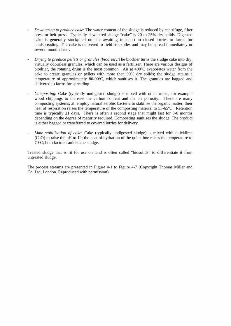
- Dewatering to produce cake: The water content of the sludge is reduced by centrifuge, filter press or belt press. Typically dewatered sludge “cake” is 20 to 25% dry solids. Digested cake is generally stockpiled on site awaiting transport in closed lorries to farms for landspreading. The cake is delivered to field stockpiles and may be spread immediately or several months later.

- Drying to produce pellets or granules (biodrier):The biodrier turns the sludge cake into dry,

virtually odourless granules, which can be used as a fertiliser. There are various designs of biodrier, the rotating drum is the most common. Air at 400oC evaporates water from the cake to create granules or pellets with more than 90% dry solids; the sludge attains a temperature of approximately 80-90ºC, which sanitises it. The granules are bagged and delivered to farms for spreading.

- Composting: Cake (typically undigested sludge) is mixed with other waste, for example

wood chippings to increase the carbon content and the air porosity. There are many composting systems; all employ natural aerobic bacteria to stabilise the organic matter, their heat of respiration raises the temperature of the composting material to 55-65ºC. Retention time is typically 21 days. There is often a second stage that might last for 3-6 months depending on the degree of maturity required. Composting sanitises the sludge. The product is either bagged or transferred to covered lorries for delivery.

- Lime stabilisation of cake: Cake (typically undigested sludge) is mixed with quicklime

(CaO) to raise the pH to 12; the heat of hydration of the quicklime raises the temperature to 70ºC; both factors sanitise the sludge.

Treated sludge that is fit for use on land is often called “biosolids” to differentiate it from untreated sludge. The process streams are presented in Figure 4-1 to Figure 4-7 (Copyright Thomas Miller and Co. Ltd, London. Reproduced with permission).

Figure 4-1 Process Streams for Anaerobic Digestion

SHORT-RETENTION THERMOPHILIC

AEROBIC DIGESTION

(as a liquid phase pre-sanitisation using the

heat of biological respiration possibly with supplementary heating)

SANITISATION (liquid phase pre-sanitisation using

supplementary heating)

THERMOPHILIC ANAEROBIC

DIGESTION (TAnD)

ACID REACTOR (mesophilic or thermophilic)

MESOPHILIC ANAEROBIC DIGESTION

(MAD)

SECONDARY DIGESTION

Post Digestion Storage

SLUDGE WELL Primary, Secondary, Co-settled, etc.

(MODULE 2)

SOURCE CONTROL (MODULE 1)

Post Stabilisation Dewatering MODULE 4

M O

D U

L E

3

Sanitised MAD

Liquid


(MAD)


(MAD)

MAD Liquid

Sanitised TAnD Liquid

Sanitised TAD/MAD

Liquid

METHANOGENIC REACTOR (mesophilic)

2 Phase Anaerobic Digested

THERMAL HYDROLYSIS

e.g. ‘CAMBI’


(MAD)

Sanitised MAD

Liquid

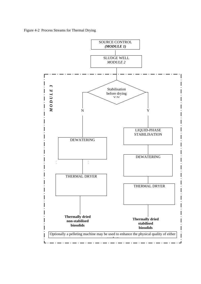
Figure 4-2 Process Streams for Thermal Drying

SLUDGE WELL MODULE 2

DEWATERING

THERMAL DRYER

Optionally a pelleting machine may be used to enhance the physical quality of either product

Thermally dried non-stabilised

biosolids

Thermally dried stabilised biosolids

THERMAL DRYER

DEWATERING

M O

D U

L E

3

LIQUID-PHASE STABILISATION

N Y

Stabilisation before drying

Y/N

SOURCE CONTROL (MODULE 1)

Figure 4-3 Process Streams for ‘Low Technology’ Outlets Only small quantities are treated by these processes, or they are not currently of great operational significance

SLUDGE WELL MODULE 2 – could also be exit biosolids from other MODULE 3

REED BEDS VERMICULTURE (on porous

support medium)

DEWATERING

VERMICULTURE

Stabilised Cake

Stabilised Cake

Stabilised Cake

DRYING BEDS (possibly with

sanitisation by solar conditioning)

Stabilised Cake

LONG-TERM CONTROLLED LAGOONING

Stabilised Liquid

M O

D U

L E

3

Y N

Stabilisation by MAD

Y/N

Figure 4-4 Process Streams for Stabilisation by Thermophilic and Autothermic Thermophilic

Aerobic Digestion (TAD & ATAD) SLUDGE WELL

MODULE 2

ATAD TAD (long enough retention to achieve

stabilisation / vector attraction reduction as distinct from short-

retention TAD-pre-MAD)

Sanitised ATAD Liquid

Thickener

Sanitised TAD Liquid

MO

DU

LE

3

Post Stabilisation Dewatering

MODULE 4

Figure 4-5 Process Stream for Composting


DEWATERING

MIXING

COMPOSTING

(Window, Aerated Static Pile, In-Vessel)

SCREENING

MATURATION

Composted biosolids

BULKING AGENT (straw/woodchips/greenwaste)

FINES

OVERSIZE

CONTRAS TO WASTE OR

RECYCLE THROUGH PROCESS

M O

D U

L E

3

Composted materials are conventionally sold after maturation, but a market is emerging forimmature compost because it has enhanced disease control effects compared with fullymatured compost, it may also have greater nutrient content

Mature Immature

Mature or immature compost?

Figure 4-6 Process Streams for Alkaline Stabilisation


DEWATERING

SYSTEMS USING PROPRIETARY

ALKALINE ADMIXTURE FOR pH

& HEATING FROM HEAT OF

HYDRATION (e.g. Rhenipal, N-Viro)

SLAKED LIME ADDITION (to liquid)

SYSTEMS USING QUICK LIME

ADDITION TO CAKE FOR pH & HEATING FROM

HEAT OF HYDRATION

Lime Stabilised

Liquid

Lime Stabilised

Cake

SYSTEMS USING QUICK LIME FOR pH & SOME HEAT FROM HEAT OF

HYDRATION PLUS SUPPLEMENTARY

HEAT (e.g. RDP)

Lime Stabilised

Cake

Lime Stabilised

Cake

M O

D U

L E

3

HORIZONTAL - 2 27

Figure 4-7 Process Streams for Land Appraisal, Transport, Application and Land Use (Post-Application) – Modules 5 To 7

Biosolids from Module 2, 3 or 4

Customer registration

Deliver to site & store/stockpile

Apply to land

Assess site and calculate application rate

MO

DU

LE

7

MO

DU

LE

6

MO

DU

LE

5

Grow and harvest

crops or graze

Amenity horticulture

Land restoration

Silviculture

4.2 Composting

4.2.1 The composting process Commercial composting is the same process of decomposition that happens in the natural environment when living organisms and plants die and break down aerobically except that the scale is larger and the conditions are controlled, which speeds up the process. Composting is autothermic, thermophilic aerobic microbial stabilisation of organic matter. Typically the microbial heat of respiration raises the temperature of the composting material to >55ºC. Some of the organic matter is converted to CO2 and water. The temperature, reduction of food supply, competition, predation and chemical environment sanitise (including weed seeds and propagules) the composted material and prevent regrowth. Any organic material can be stabilised by composting provided that there is sufficient moisture and nutrients to support microbial activity. The process starts with the growth of mesophilic microorganisms when the compost is cool. This biological activity generates heat and the temperature within the compost rises. When it exceeds about 40ºC thermophilic microorganisms start to grow and take over from the mesophilic microorganisms and the temperature continues to rise. When the easily metabolised materials have been decomposed the temperature of the compost gradually falls, thermophilic microorganisms die and mesophilic organisms increase in number. At the end of the process, the material in the compost heap is so degraded that any change has become extremely slow. At this point the compost can be regarded as mature. For some uses fully matured compost is essential but for others a lesser degree of maturity is desirable. The temperature and length of time required by legislation differ between jurisdictions. The minimum time for composting is about 3 weeks because of the limitations on microbial growth.

4.2.2 Feedstocks - Green waste

- Green waste from gardens and parks - Sewage sludge - MSW (municipal solid wastes)

- Food and food residues from households and public buildings - Residues from fruit and vegetable markets

4.2.3 Green Waste Composting The feedstock is plant material comprising garden waste collected at kerbside or municipal recycling sites, from landscape gardening or forest management. The material is litter picked to remove non-plant material, such as plastics and treated wood, which would affect the finished product. The plant material is then shredded to improve the efficiency of the composting process. When the composting process is complete the material is screened and transferred to a maturing area. The mature compost is either bagged for sale to garden centres or loaded into the lorries of landscape gardeners, farmers, land restorers, etc.

4.2.4 Co-composted sewage sludge The feedstock is dewatered, digested sewage sludge (cake) and plant material, for example wood chippings. The wood chippings are mixed with the cake in roughly equal quantities. The mixture is transferred to bins, windrows or piles for composting. Once the composting process

HORIZONTAL - 2 29

is complete the material is screened and transferred to a maturing area. Oversize material may be rejected as waste or fed back into the composting process. The matured compost is either bagged of sale to garden centres, or loaded into covered commercial vehicles.

4.2.5 Composting organic fraction of MSW The organic fraction of municipal solid waste (OFMSW) comprises food waste for homes, restaurants, kitchens, canteens, etc. and from stores. It might also contain waste from fruit and vegetable markets. Waste from kitchens (of all types, except those that are strictly vegetarian) are classified as “catering waste”, which is part of Category 3 waste under the Animal By-Products Regulation (EC, 2002). This requires that composting is in an enclosed system that ensures there is no access for vermin or birds and that the minimum specified temperature is achieved in every part of the composting material. The Regulation also requires that the ‘dirty’ (reception, etc.) area of the composting site is separated from the ‘clean’ area and that people and machinery passing from ‘dirty’ to ‘clean’ undergo sanitary precautions as they would in a food factory. The Regulations require that the maximum particle size of catering waste is reduced to 12mm prior to composting and that it achieves at least 70ºC for at least 1 hour during the process; national rules that achieve an equivalent outcome are permitted. The Regulation defines microbiological limits for assessing equivalence of processes, however sampling and analysis are not defined. OFMSW has quite a high moisture content and (especially when the particle size has been reduced to <12mm) requires bulking agent to maintain adequate air porosity. There is normally an adequate supply of nutrients. Almost inevitably there will be some physical impurities (plastic, glass or metal) irrespective of how well the waste might have been separated at source and therefore some post-composting separation (screening, air-classification, ballistic separation, etc.) is undertaken to ensure the composted material is fit for use on land. Screening may also be undertaken to recycle bulking agent.

HORIZONTAL - 2 31

Feedstock

•Municipal Solid

Wastes

•Green waste

•Fruit and Vegetable

Waste

•Sewage sludge

Prepare

• Shred

• Combine

Composting

•Windrow

•Pile

•Bin

•Tower

•Tunnel

Turn Post-compost

Mature

Bag Truck

Compost

Waste

MagneticSeparator

Classifier

Figure 4-7 Elements of the composting process

HORIZONTAL - 2 33

4.3 Paper Mill Sludge

4.3.1 Feedstock Within Europe the main producers of virgin pulp for papermaking are Finland and Sweden. The main primary paper producers are Germany, Finland, Sweden and France. Virgin pulp is imported from outside the United Kingdom for the production of white paper but a high proportion of paper production is from recycled paper. Feedstock to paper recycling plants depends on the quality of the paper that is being manufactured. High quality recycled pulp can be produced from office paper, including photocopier paper, and glossy magazine paper that has been heavily inked. The paper is collected from businesses via waste paper merchants and waste management companies. In the UK, about 5% of high quality recycled pulp production is from paper collected from the public via recycling bins. The quality of the pulp produced depends on the length of the fibres. Each time paper is processed the fibres become shorter, reducing the quality of the recycled product.

4.3.2 Processing Virgin pulp is produced by chemical, semi-chemical or mechanical methods to break down the fibrous cellulose materials into component fibres. The properties of pulps vary depending on the production process, the wood raw material and the grade of paper wanted. In the chemical pulp production process wood chips are mixed with chemicals and heated in a digester to selectively dissolve the lignin and make it soluble. Two different processes are used to produce chemical pulp, namely the sulphate (kraft) process or the sulphite process. The production process includes a recovery process where the chemicals are separated from the pulp and recycled within the system. The kraft process can be used for almost any wood, even quite resinous species, and produces a pulp with strong fibres. The cooking liquor is alkaline, an aqueous solution of sodium hydroxide and sodium sulphide. After 2 to 4 hours almost 90 % of the wood lignin is solubilised and the pulp is separated from the black liquor: a mix of the pulping chemicals and wood waste. The resulting pulp is dark brown in colour. The resulting paper is strong but brown and is used for making grocery bags, multi-wall sacks, and corrugated cartons. For white printing paper, the pulp is bleached. In the sulphite pulp process the cooking liquor is acidic or neutral. Typically the raw material is less resinous softwood chips, mostly spruce. Birch, beech and aspen can also be used but pine is not very suitable. The woodchips are cooked in magnesium, calcium or ammonium bisulphite with excess sulphur dioxide present. The process yields pulps with relatively high cellulose content and good bleaching properties. The pulp produced is made up of longer, stronger and more pliable fibres and is favoured where strength properties are particularly important. Mechanical pulp is made by grinding logs against a revolving abrasive stone. The process is mostly used with low density softwood species, although some of the softer hardwoods are also processed in this way. Mechanical pulping provides 80-90% recovery of total fibre and uses fewer chemicals. Paper derived from mechanical pulps, tends to be denser and is often a component of newsprint and other printing papers.

In the paper recycling process, the waste paper feedstock is pulped and undergoes coarse screening and scrubbing to remove pins, staples and adhesives, before the de-inking stage. The pulp is de-inked by mixing with a surfactant to remove the ink. The slurry formed is siphoned off (de-inking sludge). The residue goes through a process of fine screening, washing, dispersing, non-chlorine bleaching. Depending on the quality of the feedstock and the quality of the paper to be produced, the pulp may go through the de-inking stage twice more. A comprehensive triple de-inking process ensures that 99.5% of all ink is removed. De-inking sludge is disposed or used for energy production and is not recycled. Paper production leaves a residue, including fibre, which requires treatment. Small mills dispose of this waste stream to sewer. Large mills may have their own effluent treatment plant, or transfer the effluent to a dedicated contractor. Effluent treatment results in wastewater and ‘paper mill’ sludge. This is rich in carbon and can be recycled as soil improver. Generally, sludge is produced at two steps in the process of treating the effluent. Primary clarification is usually carried out by sedimentation, but may be carried out by dissolved air flotation. Secondary treatment is usually a biological process similar to that in sewage treatment. The resultant ‘paper mill’ sludge is then mixed with the primary sludge prior to dewatering and use or disposal.

4.3.3 The quality of ‘paper mill’ sludge The quality of the sludge depends on the raw materials, the production processes and the final product. The amount of residue produced for each grade of paper depends, in part, on the sources of the raw material. The effluent from virgin paper production contains less fibre than other paper sludges and has a greater mineral content. In general kraft pulp mill sludge (i.e. from softwood pulp) tends to have a greater sulphur content and de-inking mill sludge has a greater ash content. The heavy metal content of de-inking sludge is higher than other paper sludges.

Mills that use recycled fibre as feedstock have more residuals to dispose of than mills that use virgin pulp. This is partly due to fillers in the paper that for the most part are not recovered. The temporal variability of sludge reflects the consistency of the feedstock. In general the variation in the sludge produced by a single mill is much less than the variation between mills; because of attenuation of variation from the feedstock through the production process. The characteristics of the sludge depend on the wastewater technology used in the mill, which can involve different physical, chemical, thermal and biological treatments. The sludge is dewatered to produce cake with up to 40% DS. Dewatered cake is not aged in the same way as compost.

4.3.4 Paper mill sludge end uses Paper mill sludge has several end uses or it might be disposed in landfill. It may be burnt for power generation, reused (e.g. animal bedding, oil absorbent materials, egg cartons), applied to land as a soil amendment or used as an ingredient for compost. The use of paper mill sludge on land is controlled by National and/or regional legislation. When it is used on land, paper mill sludge is usually dewatered. There are differences in sampling for production control and regulatory purposes. For production control purposes sludge samples might be collected from the conveyors after dewatering. For regulatory purposes it is more likely that the heaps of sludge cake would be

HORIZONTAL - 2 35

sampled. If a mill is producing a wide range of products, or the production rate increases, sampling might be more frequent. Random samples would be taken from the heap and mixed to form a composite. These would be analysed for nutrients (N, P, K) and contaminants (heavy metals). Sanitary parameters are not really relevant to paper sludge.

4.3.5 Recycling Practice in the United Kingdom In the United Kingdom paper mill sludge cannot be applied to agricultural land without agreement from the Environment Agency. Once agreement to spread has been reached with a farmer, the fields for spreading are surveyed. The field is walked in a ‘W’ and at least 20 samples are taken with a trowel or corer. These are bulked together to form a composite sample, which is sent for analysis. Soil analysis is carried out every time application is planned, typically alternate years, occasionally annually. This is a requirement of the paper sludge exemption licence. Using the analytical data for the soil and sludge and groundwater data, an application rate is calculated. The sludge application rate is based on the nutrient content of the sludge, but constrained by the heavy metal content and groundwater protection requirements. An Environmental Assessment is produced and sent with pre-notification to the Environment Agency. Once this has been agreed the sludge is transported to the farm, where it is stockpiled prior to spreading on the fields.

5 EXISTING STANDARDS OR DRAFT STANDARDS

5.1 Introduction

In some cases, although specific standards for a material are not available, procedures contained in other standards may be appropriate. For example, ISO 11648-2, Statistical aspects of sampling from bulk materials: Sampling of particulate materials, does not specifically mention sludge granules. However, sludge granules are particulate materials, so the general principles in ISO 11648-1 and the statistics contained in ISO 11648-2 are appropriate to this material. Standards Bodies produce documents which have a range of status:

• Standards which are prescriptive and written in an instructive context (ISO – International Standards; EN – European Standards; dual prefix for joint adoption; some Standards may carry only a National prefix, e.g. BS – United Kingdom, DIN – Germany)

• Guidance which are advisory, normally providing an element of recommendation and example

• Technical Reports which are informative (TR – ISO; CR – CEN) Publication status of documents is indicated by the following prefixes:- FDIS – Final Draft International Standard (ISO) prEN – Pre-publication Draft European Norm A wide range of current European and International standards were reviewed. The catalogues of the European National Standards Bodies (NSB), where available on-line in English, were consulted:

- Austria (ON) - Belgium (IBN) - Denmark (DS) - Finland( SFS) - France (AFNOR) - Germany (DIN) - Italy (UIN) - Luxembourg (SEE) - Sweden (SIS) - UK (BSI)

The catalogues of the other NSB’s were not available in English. It is important that standards are harmonised to avoid duplication of effort. Therefore the standards and work-in-progress of the CEN and ISO Technical Committees were contacted and their work reviewed:

- CEN/TC 223: Soil improvers and growing media - CEN/TC 230: Water Analysis - CEN/TC 260: Fertilizers and liming materials - CEN/TC 292: Characterization of waste. WG1: Sampling - CEN/TC 308: Characterisation of sludges - CEN/TC 335: Solid Biofuels - CEN/TC 345: Characterisation of Soils - CEN/TC 134: Fertilizers and Soil Conditioners

HORIZONTAL - 2 37

- ISO/TC 147: Water Quality, Subcommittee 6, WG11, Sampling of sediments and sludges

- ISO/TC 190: Soil Quality

5.2 Technical committees

5.2.1 CEN/TC 223: Soil improvers and growing media There is active international trade in soil improvers and growing media. The purpose of CEN/TC 223 is to facilitate trade in soil improvers and growing media by enabling harmonised declaration and labelling through standards. Soils in situ are excluded from the scope. Materials in bulk and in bags are included. The uses for soil improvers and growing media include agriculture, horticulture (professional plant growing), gardening and landscaping. Soil improvers are materials, which may have been composted or otherwise processed, that are added to soil mainly to improve its physical condition without causing harmful effects. Materials that are co-composted with sludges and biowaste, which are within the scope of this report, may be used as soil improvers. WG3, Sampling methodologies, reported that no ISO standards existed specifically for soil improvers and growing media. Work in related areas, for example ISO/TC 190, Soil Quality, was considered by the working groups in order to harmonize the work and avoid duplication. Two European standards have been produced for sampling of soil improvers and growing media: EN 12579:2000 Soil improvers and growing media. Sampling EN 12580:1999 Soil improvers and growing media. Determination of a quantity In some countries the national implementation of these standards are cited in legislation dealing with soil improvers and growing media. They therefore have legal and commercial significance.

5.2.2 CEN/TC 230: Water Analysis The objectives of CEN/TC 230 are the elaboration of standard test methods for physical, chemical, biochemical, biological, microbiological examination of water quality including methods for sampling, quality assurance, and classification aspects. CEN/TC 230 works in close cooperation with ISO/TC 147 on standardization in the area of water analysis including: - definition of terms; - sampling of water; - measurement; - reporting. Excluded are the limits of acceptability for water quality.

5.2.3 CEN/TC 260: Fertilizers and liming materials The standards cover solid fertilizers and liming materials in packages up to and including 50 kg in mass or in bulk, provided the product is being moved. Products in intermediate bulk containers, holding up to 1000 kg, may be treated as packages or in bulk. The standards do not cover static heaps of a product and do not include statistical sampling plans. As is the case with CEN/TC 223 (above) there is active international trade in fertilisers and liming materials. There have been regulations dealing with purity and declaration for more than 150 years. Standards are cited in legislation and therefore have legal and commercial significance.

5.2.4 CEN/TC 292: Characterization of Waste. WG1: Sampling. Any biomaterial (biowaste, sludge, etc.) that is rejected due to failure to reach the standards may be put to landfill. Therefore it is important that account is taken of the standards for the characterisation of waste materials when designing a plan for the sampling of biomaterials. Failure of the biomaterials sampling scheme to meet the requirements for waste characterisation could result in duplication of the sampling effort. Technical Committee 292, Characterization of Waste, is in the process of preparing a European Standard for the sampling of waste materials. The work programme comprises a draft standard and five supporting Technical Reports (Table 5-1).

Table 5-1 The CEN/TC 292 Working Group 1 Work Programme (as at March 2003) WI No. Project reference Title WI 292002 Pr ENV xxxx Sampling of waste materials: Framework for the preparation

and application of a sampling plan

WI 292001 TR xxxx Part 1 Sampling of liquid and granular waste materials including paste-like materials and sludges – Technical Report xxxx Part 1: Selection and application of criteria for sampling under various conditions

WI 292017 TR xxxx Part 2 Sampling of liquid and granular waste material including paste-like materials and sludges – Technical Report xxxx Part 2: Sampling techniques

WI 292018 TR xxxx Part 3 Sampling of liquid and granular waste materials, including paste-like materials and sludges – Technical Report xxxx Part 3: Procedure for sub-sampling in the field

WI 292019 TR xxxx Part 4 Sampling of liquid and granular waste materials, including paste-like materials and sludges – Technical Report xxxx Part 4: Procedures for sample packaging, storage, preservation, transport and delivery

WI 292041 TR xxxx Part 5 Characterisation of waste – Sampling of waste materials – Guidance on the process of defining the Sampling Plan

5.2.5 CEN/TC 308: Characterisation of sludges The remit of this committee includes sludges from wastewater treatment works, water treatment works and industrial processes. The methodologies are also applicable to sludges with similar characteristics, e.g. septic tank sludges. The corresponding International body dealing with sampling is ISO/TC 147, Subcommittee 6, WG11, Sampling of sediments and sludges. The sampling standards have been produced, but without statistics, and are directly applicable to the materials covered by this report.

5.2.6 CEN/TC 335: Solid Biofuels The Technical Committee CEN/TC 335 Solid Biofuels was established in 2000. It’s scope includes drafting of standards for solid biofuels originating from: products from agriculture and forestry; vegetable waste from agriculture and forestry; vegetable waste from the food

HORIZONTAL - 2 39

processing industry; wood waste (with the exception of wood waste that may contain halogenated organic compounds or heavy metals as a result of treatment); treated wood originating from building and demolition waste; cork waste. Working Group 3 is concerned with the elaboration of two standards: Solid Biofuels: Sampling and Solid Biofuels: Sample reduction.

5.2.7 CEN/TC 345: Characterisation of Soils The remit of this recently established Technical Committee is standardisation for the characterisation of soils e.g. sampling, measurement and reporting. Excluded are the definitions of limits of acceptability for soil pollution and civil engineering aspects.

5.2.8 ISO/TC 134: Fertilizers and Soil Conditioners ISO/TC 134 is the International body corresponding to CEN/TC 260. The responsibility of this TC is standardization in the field of fertilizers and soil conditioners, that is, materials whose addition is intended to ensure or improve the nourishment of cultivated plants and / or to improve the properties of soils. Subcommittee 2 of this TC is concerned with sampling. Its standards on sampling and statistics were the foundation for CEN/TC 260’s sampling standard.

5.2.9 ISO/TC 147 Water Quality The remit of this Technical Committee is standardization in the field of water quality, including definition of terms, sampling of waters, measurement and reporting of water characteristics. Subcommittee 6 of this TC is concerned with sampling (general methods). Within this Subcommittee, Working Group 11 deals with sampling of sediments and sludges.

5.2.10 ISO/TC 190: Soil quality An equivalent European committee, CEN 345, has recently been formed (see above). Subcommittees SC1, Evaluation criteria, terminology and codification, has produced a standard, ISO 11074 in four parts. Relevant to this report is Part 2: Soil quality. Terminology and classification. Terms and definitions relating to sampling. Subcommittee SC2, Sampling, has produced a standard, ISO 10381 in 8 parts. Relevant to this report are: - Part 1: Guidance on the design of sampling programmes - Part 2: Guidance on sampling technique - Part 3: Guidance on safety - Part 4: Guidance on the procedure for investigation of natural, near-natural and

cultivated sites - Part 6: Handling and storage for aerobic microbial processes

5.3 Sampling approaches – Guidance based on Standards

Table 5-2 lists the standards and related documents reviewed in the preparation of this study. There are many aspects of the sampling process which are addressed in more than one of the standards listed although they may be dealing with different materials. These standards provide a very wide range of guidance on most aspects of the sampling process including, health and safety, sampling tools, numbers of samples, sampling plans, and analysis and interpretation of data. In the following sections relevant aspects of the sampling process are briefly discussed. In each section reference is given to the standards which provide guidance most appropriate to the materials and environments considered in this study. The procedures

followed in the experimental investigations follow the conclusions of the methods and approaches reviewed in these sections.

Table 5-2 European, International and National standards consulted in this report Standard Number Title BS 812-101:1984

Testing aggregates. Guide to sampling and testing aggregates

BS 1017:Part 2:1960 The sampling of coal and coke. Sampling of coke

BS 1017-1:1989 Sampling of coal and coke. Methods for sampling of coal

BS 1017-2:1994 Sampling of coal and coke. Methods for sampling of coke

ISO 1213-2:1992

Glossary of terms relating to sampling, testing and analysis of solid mineral fuels

ISO 1464:1994

Soil quality. Chemical methods. Pretreatment of samples for physico-chemical analyses

EN 1482:1996 Sampling of solid fertilizers and liming materials

ISO 1839-1980

Method for sampling tea

ISO 2584:1976 Statistical interpretation of data- Techniques of estimation and tests relating to means and variances

ISO 2602-1975 Guide to statistical interpretation of data. Part 2: Estimation of the mean confidence interval

BS 2846-1:1991

Guide to Statistical interpretation of data – Part 1: Routine analysis of quantitative data

BS 2975:1988

Methods for sampling and analysis of glass-making sands

ISO 3081-1986 Iron ores- Increment sampling- manual method

ISO 3082:2000

Methods of sampling iron ores. Sampling and sample preparation procedures

ISO 3084-1986

Evaluation of sampling methods for iron ores. Experimental methods for evaluation of quality variation

ISO 3085-1986

Evaluation of sampling methods for iron ores. Experimental methods for checking the precision of sampling

ISO 3085:2000

Iron ores. Experimental methods for checking the precision of sampling, Sample preparation and measurement

ISO 3086:1998

Iron ores. Experimental methods for checking the bias of sampling

EN ISO 3171 Petroleum liquids. Automatic pipeline sampling

HORIZONTAL - 2 41

Standard Number Title ISO 3534-1977

Statistics – Vocabulary and symbols

BS 3680-10C:1996 Measurement of liquid flow in open channels. Sediment transport. Guide to methods of sampling of sand-bed and cohesive-bed materials

BS 3680-3Q:2002

Measurement of liquid flow in open channels. Guidelines for safe working practice in river flow measurement

ISO 3963:1977 Fertilizers- Sampling from a conveyor by stopping the belt

BS 4103 Part 1:1967

Methods for the sampling of manganese ores. Manual sampling

ISO 5306:1983 Fertilizers – Presentation of sampling results

ISO/TR 5307:1991 Fertilizers- Part 2: Sampling- Section 2.6: Guide to derivation of a sampling plan for the evaluation of a large delivery of solid fertilizer

ISO 5308:1992 Fertilizers. Part 2: Sampling- Method of checking the performance of mechanical devices for sampling of solid fertilizer moving in bulk

BS 5309-1:1976

Methods for sampling chemical products. Introduction and general principles

BS 5309-4:1976

Methods for sampling chemical products. Sampling of solids

EN ISO 5667-3:1996 Water quality- Sampling- Part 3: Guidance on the preservation and handling of samples

EN ISO 5667-13:1998 Water quality- Sampling- Part 13: Guidance on sampling of sludges from sewage and water treatment works

ISO 5667-15:1999 Water quality – Part 6: Sampling – Section 6.15: Guidance on preservation and handling of sludge and sediment samples

ISO 5667-17:2000

Water quality. Sampling. Guidance on sampling of suspended sediments

BS 6200-5:1997

Sampling analysis of iron, steal and other ferrous metals. Guidelines on statistical procedures

ISO 6644:2002

Flowing cereals and milled cereal products. Automatic sampling by mechanical means

ISO/TR 7553:1987 Fertilizers- Sampling- Recommendations for minimum mass of increment of a solid fertilizer to be taken to be representative of the total sampling unit

ISO 7742:1988 Solid fertilizers- Reduction of samples

Standard Number Title

ISO 8358:1991

Fertilizers. Sampling. Methods for preparation of samples of solid fertilizer for chemical and physical analysis

ISO TR 8550:1994

Guide for the selection of an acceptance sampling system, scheme or plan for inspection of discrete items in lots

ISO 8633:1992 Fertilizers- Part 2: Sampling. Section 2.1 Simple sampling method for small lots of fertilizer

ISO 8634:1991 Fertilizers- Part 2: Sampling- Section 2.9 Sampling plan for the evaluation of a large delivery of solid fertilizer

ISO 8656-1:1988

Refractory raw materials. Method of sampling

BS 10175:2001 Investigation of potentially contaminated sites. Code of practice

ISO 10381-1:2002 Soil quality – Sampling- Part 1: Guidance on the design of sampling programmes

ISO 10381-2:2002 Soil quality- Sampling- Part 2:Guidance on sampling techniques

ISO 10381-3:2001 Soil quality- Sampling- Part 3: Guidance on safety

ISO/FDIS 10381-4:2002(E) Soil quality- Sampling- Part 4: Guidance on the procedure for investigation of natural, near-natural and cultivated sites

ISO 10381-5 Soil quality. Sampling. Part 5: Guidance on investigation of soil contamination of urban and industrial sites

ISO 10381-6:1993

Soil quality. Sampling. Guidance on the collection, handling and storage of soil for the assessment of aerobic microbial processes in soil

ISO/DIS 10381-8 Soil quality- Sampling- Part 8:Guidance on the sampling of stockpiles

ISO/DIS 10978 Fertilizers- Sampling- Part 2: [New section] Solid fertilizer sampling from a bulk stream

ISO 11074-2:1998 Soil quality – Part 1: Terminology and classification- Section 1.2: Terms and definitions relating to sampling

ISO 11648-2:2001 Statistical aspects of sampling from bulk materials- Part 2: Sampling of particulate materials

EN 12255-8:2001 Wastewater treatment plants – Part 8: Sludge treatment and storage

EN 12579:1999 Soil improvers and growing media- Sampling

HORIZONTAL - 2 43

Standard Number Title EN 12580:1999 Soil improvers and growing media- Determination of

quantity

EN 13040:1999 Soil improvers and growing media- Sample preparation for chemical and physical tests, determination of dry matter content, moisture content and laboratory compacted bulk density

CR 13455:1999 Soil improvers and Growing Media – Guidelines for the safety of users, the environment and plants.

CR 13097:2001 Characterization of sludges – Good practice for utilization in agriculture

CR 13456:1999 Soil improvers and growing media – Labelling, specifications and product schedules

ISO 13909-3:2001

Hard coal and coke. Mechanical sampling. Coal. Sampling from stationary lots

ISO 13909-7:2001

Hard coal and coke. Mechanical sampling. Method for determining the precision of sampling, sample preparation and testing

ISO 13909-8:2001

Hard coal and coke. Mechanical sampling. Methods of testing for bias

ISO 14507:2003 Soil quality- Pretreatment of samples for determination of organic contaminants

ISO 16269-7:2001 Statistical interpretation of data- Part 8: Median- estimation and confidence intervals

EN 25667-1:1994

Water quality- Sampling- Part 1: Guidance on the design of sampling programmes

EN 25667-2:1993 Water quality – Sampling – part 2: Guidance on sampling techniques

ISO/FDIS 5667-19:2003(E) Water quality – Sampling methods – Part 19: Guidance on sampling of marine sediments

5.4 Health and safety

Documents dealing with Health and Safety aspects of sampling make the following points:

5.4.1 General There is a wide range of conditions encountered in sampling biomaterials and soil. The hazards associated with the various situations that may be encountered in sampling practice may affect the choice of sampling site. Personnel responsible for designing sampling programmes and for carrying out sampling operations should ensure that the requirements of relevant (inter)national regulations and site specific safety instructions are taken into account. Sampling personnel should be informed of the necessary precautions to be taken in sampling operations. This should include safe working practices for specific locations, the use of protective clothing and equipment, decontamination and emergency procedures. The sampler should comply with any health and safety instructions whilst on the site. The most comprehensive guidance on safety is given in ISO 10381-3 (Soil quality- Sampling- Part 3: Guidance on safety). The scope of ISO 10381-3 includes general guidance on hazards that may be encountered in a site investigation, in addition to more specific guidance on site investigation on agricultural or contaminated areas and geological investigations. More specific information on general health and safety aspects on sampling biomaterials is given in other standards. There are three areas where safety during sampling is an issue. Hazards can be presented by:

- the material being sampled, e.g. compost, sludge; - the sampling location, e.g. vehicles, ground surface; - the sampling situation, e.g. piles, conveyors.

5.4.2 Hazards presented by exposure to the materials being sampled In the process of sampling biomaterials hazards can be grouped into three main categories: Traumatic hazard This hazard concerns abrasion, cuts and wounds provoked by sharp objects. Particles can be sharp portions of the product itself (splinters, debris, fibres, coarse particles) or impurities such as glass, metal debris, or damaged containers. Typically a maximum allowed limit of impurities, such as glass and metal of a given size, is defined for composted waste, which presents the greatest risk of sharp impurities. Organic fibres and coarse abrasive materials can pose a hazard of skin lesion or irritation of the eye, and minor skin irritation, often connected with the dust fraction. Biological hazard Microorganisms may be present in the feedstock or could contaminate or grow in organic materials during their production and storage. Some of these can cause infection and others, especially moulds and actinomycetes, can cause allergy or other diseases either directly or through their products. Infection occurs through ingestion of contaminated material, penetration of skin though open wounds, puncture and scars. Inhalation of organic dust or aerosols also presents a hazard.

HORIZONTAL - 2 45

Dust The hazard is generated by the presence of airborne particulate matter. For materials containing fine particles, such as composted green waste, dust is a property of the material. For others, such as sludge granules, abrasion during handling may produce dust. Dust represents a hazard via inhalation (upper respiratory tract irritation) of inhalable dust, eye and skin contact (minor abrasion), and penetration through open wounds. Dust has also been associated with a biological hazard of allergic sensitisation or reaction in sensitive individuals.

5.4.3 Hazards presented by the sampling location and situation While general safety concerns are covered in the standards for sampling, they are not always detailed. Safety issues will be specific to the site where sampling it carried out. The provisions of national health and safety regulations should always be carefully studied and put into effect before sampling occurs. Sampling from a conveyor by stopping the belt (where the principle is to move everything from a defined length of belt) is the reference method for sampling of solid fertilisers and liming materials to assess the accuracy of other techniques. It is not recommended for regular use because it is time-consuming and interrupts the loading or unloading process. Safety warnings are given in ISO 3963:1977 and EN 1482:1996. This sampling method (stopped belt) involves contact with machinery which is normally in motion. It is essential that precautions be taken so that there is no possibility of the conveyor starting up while the increments are being taken. An override start/stop button should be provided at the point of sampling. The sampler should be able to reach the whole cross-section of the belt without undue physical strain. The position of sampling should be made as convenient as possible, for example by using a suitable platform. EN ISO 5667-13:1997 includes a section for the safe collection of sludge samples from sewage and water treatment works (Section 7 Safety). Examples of the type of risk that may be present with respect to sludge sampling in particular are given:

- Slippage on wet flooring - Bacterial and parasitic infection - Dangerous atmospheres (explosion, oxygen deficiency) - Flooding (sewers and holding tanks) - Slippage or sinking (sampling from stockpiles) - Moving machinery (belts and press plates) - Aerosols - Size of sample (maximum mass to be lifted)

Some of the safety precautions listed in ISO 5667/1-1980 may be relevant to some sludge sampling situations, for example sampling from lagoons. The use of electrically operated sampling equipment in or near water can present electrocution hazards. Weather conditions should be considered and life-jackets and life-lines should be worn. Reasonable access in all weather is important and it is essential for frequent routine sampling. There are risks associated with sampling that are products of the sample handling procedure for example the addition of preservatives to stabilise certain physical and chemical constituents (EN ISO 5667-13). Certain preservatives need to be used with caution, considering the danger involved in their handling. Operators should be warned of these dangers and the ways of protecting themselves from them.

Often special safety instructions / regulations are in effect at industrial sites. Some additional safety instructions, specific to industrial sites, are given in ISO 10381-8. Where (large) stockpiles are part of the (industrial) activities, heavy mechanical equipment can pose an additional threat to the sampler. Operational personnel should be informed about the presence of the sampler on site. No specific safety reference was found to sampling of sludge cake in heaps or stockpiles. ISO 10381-8 cautions that, when sampling non-consolidated stockpiles, the sampling plan should contain additional safety instructions on how the stockpile shall be sampled safely.

5.5 Sample Preservation, Labelling and Handling

5.5.1 General Samples may be collected for chemical (inorganic, organic), physical or biological (including microbiological) examination or some combination of these. Methods of sampling and preservation of samples for each examination may differ greatly. Therefore storage of the samples, including methods and speed of transport to the investigation laboratory, should be carried out in accordance with the requirements of the aim of the investigation and the desired accuracy of the analytical results. The sampler should never have to obtain samples without having an idea of what they are intended for. Full details of the transport and storage conditions should be recorded (e.g. temperature, light, humidity, type of container, duration of transport, etc.). Unless there is a mobile field laboratory, analysts are rarely present at the site. In some situations, this has the disadvantage that samples reaching the laboratory may not reflect the original chemical state of the site. Every effort should be made to preserve and ensure the integrity and identity of the sample after sampling and until it reaches the laboratory. In general, the sample container should be inert, relatively inexpensive and convenient to use. For sampling uncontaminated soil, containers made from polyethylene (such as buckets, wide-mouthed bottles and strong bags) may be used. However, these may not be suitable if the analytical requirements were for organic solvents or volatile compounds. Suitable packing should: - Preserve the components of the sample that are to be examined; - Prevent cross-contamination either between samples or from the environment; - Prevent loss of sample, for example by leakage from bottles or tearing of bags; - Be appropriate for the size of sample to be collected; - Preserve the structure of the sample in the case of undisturbed samples. Samples should be stored in such a manner that the sample is preserved and guarded from cross-contamination or loss of sample. The storage time between sampling and laboratory analysis should take into account the components of the sample that are to be examined.

5.5.2 Labelling It is essential that samples are labelled and described adequately, including any special instructions for the laboratory. It should be recognised that analytical laboratories might be processing hundreds of samples per day. They probably will not recognise the samples and the sample location names probably mean nothing to them. It is therefore vital that the samples are accompanied by all of the information that might be relevant to the laboratory and that all information that might be relevant to interpreting the results is also recorded. Many standards refer to this subject.

HORIZONTAL - 2 47

5.5.3 Soils Suitable packing, preservation, storage, transportation and delivery of soil samples are discussed in detail in ISO/DIS 10381-8 (clause 9). A list of suitable containers is shown in Table 5-3.

The method of preservation will influence the acceptable time between sampling and analysis. In general this time should be kept to a minimum to avoid sample alteration. A number of preservation methods are available for soil samples:

- Air tight storage; - Dark storage; - Cooled storage (<6oC); - Nitrogen atmosphere.

Other preservation methods are also available, like drying and freezing, but cannot be applied in the field. These are most likely to be used when analysis of the samples is likely to be delayed. The properties of organic micropollutants can differ greatly according to chemical species. Packing and preservation of soil samples for organic analysis is discussed in ISO 14507. Samples taken for organic analysis should be kept cool and processed as soon as possible. The method of pretreatment will depend on the volatility of the organic compound(s) or group(s) of organic compounds to be determined. Samples collected for the assessment of microbial processes will need different handling to minimise changes. Samples should be transported in a manner which minimises changes in the soil water content, and should be kept in the dark with free excess of air. Extreme environmental conditions should be avoided and the soil should be kept as cool as possible but not allowed to freeze, dry out or become waterlogged. The soil should be processed as soon as possible after sampling. The maximum storage time depends on the parameters to be determined and the material used for the container. The storage time depends on the possibilities of volatilisation and biological degradation. For samples containing volatile organic compounds or compounds that are subject to rapid microbial decomposition, the analysis should be carried out as soon as possible, within 1 to 2 days. It may not be possible to form composite samples for the analysis of volatile organic compounds because any mixing process may result in losses.

HORIZONTAL - 2 49

Table 5-3 Selection of sample containers suitable for soils from uncontaminated sites (reproduced from ISO/DIS 10381-8).

Suitability for use

Size variability Type of container Resistance to extreme

temperature

Cost of purchase

Resistance to breakage

Degree of water and

gas tightness

Ease of reopening

Suitability for

volatiles Small Large

Inorganic analysis

Organic analysis

Rigid plastic with screw caps or snap on lids 1)

+

++

+

-

+

-

+

+

+

-

Glass bottles or jars with plastic caps and PTFE seals 1)

+

+

-

+

+

+

+

-

-

+

Coloured plastic bottles with plastic caps and PTFE seals

+

+

+

+

+

+

+

+

+

-

Coloured glass bottles with plastic caps and PTFE seals

+

+

-

+

+

+

+

-

-

+

Heavy duty resealable plastic polythene bags 2)

-

++

+

-

+

-

+

+

+

-

++ Very suitable + May be suitable - Unsuitable NOTE 1) The use of wide neck plastic and glass bottles is preferable for soil sampling 2) Plastic bags should only be used as a last resort

Preservation methods for soil samples for different types of components to be determined and for reducing soils are given in Table 5-4.

Table 5-4 Necessary (+) preservation circumstances and measures for different types of components and soils (reproduced from ISO/DIS 10380-8).

Volatile

components Semi-volatile components

Non-volatile inorganic components

Reducing soils 1)

Air tight storage + + - +

Dark storage + + - -

Cooled storage (<6oC) 5) + + - +

Nitrogen atmosphere - - - +

Maximum period of storage 2)

< 7 7 3) < 7 4)

1) When reducing characteristics are to be maintained 2) When stored with the appropriate preservation method 3) No maximum period when dried prior to storage 4) maximum storage period depended on the airtightness of the sample container, but maximum of 7 days 5) The temperature should be 4 ± 2oC

NOTE 1 The preservation measures in Table 5-4 are to be considered as minimum measures. Additional measures may be applied (like storage for the analysis of non-volatile inorganic compounds in a cool environment). NOTE 2 The maximum period of 7 days is not validated, but based on laboratory practice. NOTE 3 Volatile components are organic and inorganic components with a boiling point under 300oC. All organic components with a boiling point above 300oC are here to be considered as semi-volatile according to ISO 14507.

5.5.4 Biomaterials The standards for sampling of solid fertilizers and liming materials do not include recommendations for packing, preservation, storage, transportation and delivery. It is likely that the recommendations for soils or other biomaterials would apply equally well to these materials because similar components would need to be examined see for example to ISO 5667-15:1999. Similarly, the standards for sampling of soil improvers and growing media (EN 13040 and EN 12579) make general recommendations only. EN 13040 states that the laboratory sample shall be transported and stored without compaction or any other treatment which may irreversibly alter its moisture content, particle size, packing characteristics or any feature which affect density. Additional comments are made on storage of samples submitted to the laboratory. EN 12579 adds that microbiological samples shall not be frozen and shall be transported in a manner whereby the samples are not subject to extremes of temperature. Also, that more than one final sample may be required for analysis of different characteristics and that the test method may specify constraints on the packaging. The standards procedures for storage, preservation and handling of sludges and waters are more comprehensive, and are referred to in EN ISO 5667-3, EN ISO 5667-13, EN ISO-5667-15 and EN ISO 5667-16.

HORIZONTAL - 2 51

Both EN ISO 5667-13 and EN ISO 5667-3 describe general considerations for the preservation of samples and appropriate containers for storage. EN ISO 5667-15 includes a table that lists recommended sample containers, preservation and storage conditions for different parameters measured in sediments and sludges. The recommendations cover methods for samples that are to be tested for physico-chemical parameters, organic and inorganic chemicals, ecotoxocological, bacteriological, microbial and ecological parameters. EN ISO 5667-16 gives practical guidance on the handling of waters in the context of biotesting, for example toxicity and biodegradation tests (but not for bacteriological examination of water). EN ISO 5667-3 is more comprehensive, including sections on preparation and filling of containers, and preservation of samples by freezing, filtration or centrifugation and addition of preservatives. EN ISO 5667-3 includes five tables of techniques generally suitable for the preservation and storage of samples for analysis. The tables are more detailed than EN ISO 5667-15. Table 2 lists the methods of preservation and the parameters they are suitable for. The other four tables list the preservation techniques:

• Table 1: Physico-chemical and chemical analysis; • Table 3: Microbiological analysis; • Table 4: Biological analysis; • Table 5: Radiochemical parameters.

5.6 Representative sampling

Correct sampling is a difficult operation, which requires great care. The need to obtain a fully representative sample for the chemical and physical testing cannot be stressed too much. Sampling plans have been produced to cover a range of quantities of fertilizer and these form the basis of other International Standards. The sampling plan given in ISO 8633 is not based on strict statistical principles and further information on the statistical theory of sampling fertilizers may be found elsewhere, for example in ISO/TR5307. Samples obtained by following the procedures described in ISO 8633 may be considered as representative of the original lot or sample portion. For fertilizers in bags, the sampling unit is a bag and the number of individual bags to be sampled is obtained from the table. In this context the bag is taken to contain no more than 50 kg, larger containers should be treated in bulk. For packages weighing 5 kg or less, the entire container is taken as the sample. For packages less than 1 kg each, it may be necessary to increase the number taken, to ensure a sufficiently large aggregate sample. Bags are selected randomly from the lot to be sampled. Table 5-5 Sampling of fertilizer products in bags (from ISO 8633:1992)

Sample portion Minimum number of sampling units

< 10 bags All bags 10 to 400 bags 10a > 400 bags 20a a As a guide, above 100 bags the number of sampling units may be taken as the square root of the total number of units present

5.6.1 Statistics ISO/TC27: Solid Mineral Fuels has considered the statistics of sampling in detail in its ISO 13909 series of standards. The financial ramifications of buying and selling coal and coke on the basis of calorific value determined on samples is easy to appreciate. Much of the following discussion is derived from these standards. ISO/TC 134 has also considered many of the statistical matters of sampling in its series of standards. ISO TR 7553 Fertiliser – Sampling – Recommendations for minimum mass of increment of a solid fertiliser to be taken to be representative of the total sampling unit provides similar information. To design a representative sampling scheme that can be used operationally the frequency of sampling and the number of samples and increments to be taken must be calculated. This can be done using information gathered during the commissioning phase of a new works or by using data from a works with similar operational practices and feedstock. ISO 13909-3 provides detailed statistical methods for calculating the number and frequency of sampling. Precision and total variance of sampling Precision and total variance of sampling is discussed in ISO 13909-3. In all methods of sampling, sample preparation and analysis, errors are incurred and the experimental results obtained from such methods for any given parameter will deviate from the true value of that parameter. While the absolute deviation of a single result from the “true” value cannot be determined, it is possible to make an estimate of the precision of the experimental results. This is the closeness with which the results of a series of measurements made on the same coal agree among themselves, and the deviation of the mean of the results from an accepted reference value, i.e. the bias of the results (see ISO 13909-8). It is possible to design a sampling scheme that, in principle, can achieve an arbitrary level of precision. The required overall precision on a lot should be agreed between the parties concerned. The theory of precision is given in ISO 13909-7. The following equation is derived:

u

VVm

u

n

V

PPTm

l

l

+

−+

=1

Equation 5.6-1

where

Pl is the estimated overall precision of sampling, sample preparation and testing for the lot at a confidence level, expressed as percentage absolute;

Vl is the primary increment variance; n is the number of increments per sub-lot; u is the number of sub-lots actually sampled; m is the number of sub-lots in the lot; Vm is the sub-lot variance; VPT is the preparation and testing variance.

For continuous sampling, equation 5.6.1is simplified as follows:

HORIZONTAL - 2 53

m

Vn

V

PPT

l

l

+= Equation 5.6.2

If the quality of a material of a type not previously sampled is required, then in order to devise a sampling scheme, assumptions have to be made about the variability. The precision actually achieved for a particular lot by the scheme devised can be measured by the procedures given in ISO 13909-7. Primary increment variance The primary increment variance Vl, depends upon the type and nominal top size of the material to be sampled, the degree of pre-treatment and mixing, the absolute value of the parameter to be determined and the mass of increment taken. ISO 13909-7 says the number of increments required for different analyses should be calculated separately using the relevant values of increment variance and the desired precision. If a common sample is required for more than one analysis, for example a suite of heavy metals, the number of increments required for that sample should be the greatest of the numbers calculated for the individual analyses. Number of sub-lots and number of increments per sub-lot The number of increments taken from a lot in order to achieve a particular precision is a function of the variability of the quality of the coal in the lot, irrespective of the mass of the lot. The lot may be sampled as a whole, resulting in one sample, or divided into a number of sub-lots resulting in a sample from each. Such division may be necessary in order to achieve the required precision. The procedure for calculating the necessary number of sub-lots is given in ISO 13909-3. Another important reason for dividing the lot is to maintain the integrity of the sample to avoid bias after taking the increment, for example, in order to minimise loss of moisture due to standing. The need to do this is dependent on factors such as the time taken to collect samples, ambient temperature and humidity conditions, the ease of keeping the sample in sealed containers during collection and the particle size of the material. It is recommended that, if moisture loss is suspected, a bias test be carried out to compare the quality of a reference sample immediately after extraction with the sample after standing for the normal time. If bias is found, the sample standing time should be reduced by collecting samples more frequently, i.e. increasing the number of sub-lots. There may be other practical reasons for dividing the lot: - for convenience when sampling over a long period; - to keep sample masses manageable. Continuous sampling First the minimum number of sub-lots required for practical reasons should be determined. Then the number of increments in each sub-lot for a desired precision can be estimated from the following equation [obtained by transposing Equation 5.6.2]:

PTl

l

VmP

Vn

4

42 −

= Equation 5.6.3

A value of infinity or a negative number indicates that the errors of preparation and testing are such that the required precision cannot be achieved with this number of sub-lots. In such cases, or if n is impracticably large, increase the number of sub-lots by one of the following means. - Choose a number corresponding to a convenient mass, recalculate from Equation 5.6.3

and repeat this process until the value of n is a practicable number. - Decide on the maximum practicable number of increments per sub-lot, ni and calculate m

from the following equation.

2

44

ll

PTll

Pn

VnVm

+= Equation 5.6.4

Adjust m upwards, if necessary, to a convenient number and recalculate n. Take n as 10 if the final calculated value is less than 10. Examples of calculations for continuous sampling from stationary lots are given in annex A of ISO 13909-3. Intermittent sampling Initially decide on the number of sub-lots, m, and the minimum number, u, required to be sampled for practical reasons. Estimate the number of increments for a desired precision in a lot from the following equation [obtained by transposing Equation 5.6.1]:

PTml

l

VVm

uuP

Vn

414

4

2 −

−−

= Equation 5.6.5

A value of infinity or a negative number indicates that the errors of preparation and testing are such that the required precision cannot be achieved with this number of sub-lots. In such cases, or if is impracticably large, increase the number of sub-lots by one of the following means. Choose a larger value for u, the number of sub-lots actually sampled, recalculate n and repeat this process until the value of n is a practicable number. Decide on the maximum practicable number of increments per sub-lot, n1, and calculate u from the following equation:

ml

PTml

VmP

VVn

Vm

u4

4

2

1

+

++

= Equation 5.6.6

Adjust m upwards, if necessary, to a convenient number and recalculate n from Equation 5.6.5. Take n as 10 if the final calculated value is less than 10. Examples of calculations for intermittent sampling from stationary lots are given in annex A of ISO 13909-3.

Common sample The amount of sample collected must be sufficient to complete all the required analyses. For example, where a sample for moisture determination is to be extracted from a common sample, the initial number of increments collected should be sufficient to provide enough material for general analysis and moisture determination. Increase the mass of each increment or the number of increments if there will not be sufficient material left after removal of the moisture sample in accordance with ISO 13909-4.

HORIZONTAL - 2 55

Methods of sampling from stockpiles - Stockpiles are best sampled when they are laid down or picked up by the method for

sampling of moving streams described in ISO 13909-2. The sampling of a stockpile in situ usually presents problems in obtaining a representative sample and may be used only if it is not practicable to sample the material as a moving stream. Stockpiles that are to be sampled from the surface must be sufficiently compacted to safely bear the weight of sampling personnel and equipment.

5.6.2 Sampling Location In general it is advisable to take samples from a point as close as possible to the place where the material being sampled changes ownership (e.g. just before the loading of a wagon or vessel). Products moving in bulk may be sampled, for example, when moving on a conveyor belt, or in an inclined conduit, or conveyor, or when falling from a spout or the end of a conveyor belt. A series of intermittently taken samples may be retained as separate increments so that the fluctuations in characteristics and composition of the lot can be assessed. Alternatively, they may be blended together and well mixed to provide a bulk sample. Separate-increment samples may also be retained as laboratory samples if the sample size coincides with requirements. Any bulk sample should always be thoroughly mixed to ensure the composition is as homogeneous as possible.

ISO 3963 describes the method for taking samples of fertilizer by sampling from a conveyor by stopping the belt. It cautions against taking a representative sample from a consignment of fertilizer by sampling from a conveyor by stopping the belt because this is time consuming and interrupts the loading or unloading process considerably. The standard states that it should be used only where other methods, such as automatic sampling or scoop sampling from a free fall, are impossible, or as a reference method to assess the accuracy of other techniques. Taking a sample The first stage in the design of the scheme is to identify the material to be sampled. Samples may be required for technical evaluation, process control, quality control and for commercial reasons by both the producer and the customer. It is essential to ascertain exactly at what stage in the material-handling process the sample is required and, as far as practicable, to design the scheme accordingly. In some instances, however, it may prove impracticable to obtain samples at the preferred points and, in such cases, a more practicable alternative is required.

Particulate materials Within the scope of this report, particulate materials include sludge granules and composted materials. In the case of sampling solid material, such as fertilizers, or sludge granules, the definitions and calculations in the standards for sampling of coal are appropriate (ISO 13909 parts 3, 7, and 8). ISO/TR 5307 provides a full description of the statistical theory of sampling of fertilizers and investigates effect of the parameters on the confidence of the sampling results. Division of lots A lot may be sampled as a whole or as a series of sub-lots, e.g. material despatched or delivered over a period of time, a ship load, a train load, a wagon load, or material produced

in a certain period, e.g. a shift. It may be necessary to divide a lot into a number of sub-lots in order to improve the precision of the results. For lots sampled over long periods, it may be expedient to divide the lot into a series of sub-lots, obtaining a sample for each. Continuous sampling In continuous sampling, every sub-lot is sampled and the same minimum number of increments is collected from each sub-lot. There are as many sample results for the lot as there are sub-lots. The mean result for the lot should be of the required precision but if it is desired to check that the required precision has been attained, it is possible to do this by using the procedures of replicate sampling described in ISO 13909-7. Intermittent sampling If material of the same type is sampled regularly, it may be satisfactory to collect increments from some of the sub-lots but not from others. This is called intermittent sampling. The same minimum number of increments is taken from every sub-lot that is sampled. The sub-lots to be sampled are chosen at random, unless it can be demonstrated that no bias, for example as a result of time-dependent variance, is introduced by choosing sub-lots systematically. Such demonstration shall be repeated from time to time and at random intervals. There are as many sample results per lot as there are sub-lots sampled, but because some sub-lots are not sampled, it is not possible to say whether the average of these results will have the required precision for the lot unless information about the variation between sub-lots is available. This can be obtained by following the procedure described in ISO 13909-7. If the variation between sub-lots is too large, it may be necessary to introduce continuous sampling to achieve the desired precision. Any use of intermittent sampling would need to be agreed between producer, user and regulator and should be recorded in the sampling report. Stationary lots ISO 13909-3 specifies procedures for the mechanical sampling of coal from stationary lots, for example from wagons, barges, ships and stockpiles. In this part, the principles and procedures for designing a sampling scheme are given, together with typical examples of applications; in addition, practices for the execution of sampling in different sampling situations are described. The methods described are limited to those on which it is possible to conduct a test for bias. Statistical methods are described in ISO 3081. Worked examples for the development of a sampling scheme for iron ores in trucks is given in ISO 3084. ISO 3085 presents the results of an experimental investigation of the procedures for sampling of iron ore: periodic systematic sampling or stratified sampling. Sludges and cake Many of the principles applied to particulate materials for determining the number of samples are applicable for sludges and cake. Specific procedures for sewage sludge are contained in EN 25667-1:1994. [Note: in this study we did not consider sampling from a tanker, but it may be appropriate to consider from a pipeline to be similar from a mixed tanker.]

5.6.3 Quality control programmes These usually involve the control of concentration of one or more determinands within defined limits. The results are required in order to decide whether immediate action is needed. The sampling frequency should therefore be chosen so that there is more than an acceptable probability of important deviations outside the control limits occurring between successive measurements. There are two primary factors that fix this frequency:

a) the magnitude and duration of deviations from the desired conditions; b) the probabilities of occurrence of deviations from the desired conditions.

HORIZONTAL - 2 57

Often, only approximate definitions of these factors will be possible, but reasonable estimates will enable a working value for the sampling frequency to be deduced. Establishment of sampling programmes The times and frequencies of sampling in any programme can be properly decided only after detailed preliminary work, in which a high sampling frequency is necessary to provide the information to which statistical techniques may be applied. If quality is subject to variations, either random or systematic, the values obtained for statistical parameters, such as mean, standard deviation, maximum, are only estimates of the true parameters and generally differ from them. In the case of purely random variations, the differences between these estimates and the true values can be calculated statistically; they decrease as the number of sample increases. Once the frequency of sampling has been decided, the data obtained should be reviewed regularly so that changes can be made as required. EN 25667-1 includes details of statistical methods applied to one statistical parameter, the mean, and assumes that the normal distribution applies. The terminology used is in accordance with ISO 3534 to which reference should be made for definitions of the terms used. For a full treatment of calculation of the mean in terms of confidence interval, reference should be made to ISO 2602. Confidence interval The confidence level is the probability that the true mean will be included within the calculated confidence interval L. A confidence interval for the mean value of a concentration, calculated on the basis of a sample with n results, and at a 95% confidence level, means that there are 95 chances out of 100 that the interval will contain the true mean. For the case in which a large series of samples are effectively taken, the frequency of cases in which the interval will include will be close to 95%. Determination of confidence interval and number of samples For a number of results n, taken at random, estimates of the true mean, ξ, and the standard �� ξ and s respectively according to the following formula:

( )

−

−=

−

−= ∑ ∑

∑= =

=n

i

n

iii

n

ii

xn

xnn

xx

s1

2

1

21

2

11

11

Equation 5.6.7

where xi represents the individual values. When n is large, s differs little from the true value ξ, and the confidence interval of ξ, calculated from some number 3) of results n, is ± K/n, where K has the value given in the table below depending on the confidence level adopted. Confidence Level, %

99 98 95 90 80 68 50

K 2.58 2.33 1.96 1.64 1.28 1.00 0.67 To estimate the mean for a given confidence interval L at the confidence level chosen, the number of samples necessary is (2Kξ/L)2 ��

samples will be required when only an estimate s is available, although this will make little difference to the value of K, if s is based on a relatively large number of samples. Random variation Random variations commonly have either a normal or a lognormal distribution. Systematic variations may be either trends or cyclic variations, and combinations of the two may occur. The nature of the variability may be different for different determinands in the same population. If random variations are dominant, times of sampling are generally not statistically important, although they may be important for quality control purposes. If cyclic variations occur, times of sampling are important, either to cover the whole cycle or to detect maximum or minimum concentrations of interest. Times of sampling should be spaced approximately equally over trend periods. In each of the above situations, the number of samples should be governed largely by the statistical considerations outlined above. If cyclic variations are either absent or small compared with random fluctuations, the number of samples to be taken need only be large enough to meet the acceptable uncertainty of the mean of a determinand at a given confidence level. For example, if normal distribution applies, according to the above, the confidence interval, L, of the mean of n results, at a chosen confidence level, is given by the formula:

n

KL

σ2= Equation 5.6.8

where σ is the standard deviation of the distribution.

5.6.4 Sampling equipment Sampling equipment should be suitable for the material and locations to be sampled. It is important that the sampling apparatus is made from materials that cannot affect the characteristics of the material being sampled. The device should be kept in good condition and not cause cross-contamination, for example rusty metal could flake and contaminate the sample. If the suitability of a device is not known its performance ought to be assessed by checking against the reference method. ISO 5308:1992 specifies a method of checking the performance of mechanical devices for sampling fertilizers moving in bulk by comparison of particle size distribution with that obtained by a reference method. In this example two series of increments, one using a mechanical device and one using a reference method, were collected from a quantity of fertilizer passing through a bulk-handling system. The means and variance of the particle size distribution of the two sets of samples were compared using Student’s t test. Bias The equipment used and the location where a sample is taken should not bias the result. However the method for obtaining the most representative sample may not be practicable. In this case alternative locations and sampling equipment should be checked for bias against the reference method (i.e. that which produces the most representative sample). The acceptable

HORIZONTAL - 2 59

bias (confidence interval) and confidence level need to be agreed before accepting an alternative sampling location or method. ISO 3086 specifies experimental methods for checking the bias of the sampling of iron ores, when the sampling is carried out in accordance with the methods specified in ISO 3081 or ISO 3082, having as reference a stopped-belt sampling method according to ISO 3081. The results obtained from the method to be checked (referred to as method B) are compared with the results of a reference method (referred to as method A) which is considered to produce practically unbiased results, from technical and empirical viewpoints. The standard includes the experimental data and the statistical analysis for the comparison of the two methods. The conclusion was that the new method performed as well as the reference method, within the confidence level and confidence interval specified, and the new method could be adopted as a routine method. The causes and minimization of bias is examined in ISO 13909-2. Test results obtained from the samples may be biased for a number of reasons. The causes of bias resulting from design and operation of the sampling equipment and the actions to be taken to minimize them are given below: - Improper design - Improper operation - Periodicity - Improper maintenance - Non-adherence to basis of sampling (time-basis or mass-basis) - Improper cleaning - Variability in flow rate of materials, e.g. pellets on a belt A wide range of different sampling devices are described in many standards. The following is to be regarded as an illustration only: Mechanical sampling devices for the sampling of material in motion: Transverse samplers (ISO 6644) These are for taking a complete section from a falling grain stream. They may be open-spout samplers, tubular samplers with openable sampling holes, or screw-type tubular samplers. Full-stream diverter samplers (ISO 6644) In this type, a flap or paddle swings to divert intermittently the entire grain stream. Rotating cup samplers (ISO 6644) With this type the falling grain stream is intermittently sampled by a cup with an outlet spout rotating on a central vertical shaft. Bucket elevator samplers (ISO 6644) These take samples of grain moving on a belt or conveyor. Buckets, on a continuous loop, remove samples from the full width of the grain stream because of the configuration of the side rollers concentrating the grain on the belt. The samples are released into the receiving hopper as the buckets move over the upper roller pivot. Valve arrangement for sampling liquid sludge under pressure (EN ISO 5667-13:1997) Liquids should be pumped through pipes of adequate size (for example, when sampling heterogeneous liquids, of minimum nominal bore 25mm) at linear velocities high enough to maintain turbulent flow characteristics. Horizontal pipe runs should be avoided. presence of

toxic liquids or fumes, or both, and the possible build-up of explosive vapours (EN ISO 5667-1:1997). Apparatus for the sampling of thick liquid sludge under vacuum (EN ISO 5667-13:1997) Manual sampling: Flat-bottomed shovel or scoop with vertical sides (ISO 8633:1992) Recommended for manual sampling for solid fertilizers. Spears (ISO 8633:1992) The use of sampling spears is not recommended for taking samples for the determination of physical properties of solid fertilizers. Spears can only be accepted for other sampling provided they can collect increments of more than the minimum mass defined in ISO/TR7553. In any case, the dimensions of the spear have to be appropriate to the characteristics of the sample portion and to the particle size of the fertilizer. Mechanical auger (ISO 13909-3:2001) It is essential that any mechanical sampler used is capable of taking full-depth samples. One such sampler is the mechanical auger. Using an auger for sampling is preferred, but is impractical in some circumstances, for example, sampling of materials of large top size. Soil Sampling: Techniques for taking soil samples are discussed in ISO 10381-2:2002. These include manually and power operated sampling tools and the excavation of trial pits. Since, in the context of this report, soil survey involves taking samples across the sampling area to estimate the mean soil properties most of these methods are not appropriate. The best practicable method would have to be relatively speedy and not alter unduly the properties of the soil being measured. Excavation of trial pits is more widely used for site investigations related to contaminated land, or to scientific investigation. More suitable for routine investigations are small auger, including hand-operated and power-operated augers. There are many types of hand auger available that have been developed to deal with different soil types and conditions. The ease of use depends on the nature of the ground to be sampled. In general they are easier to use on sandy soil than other soil, particularly where obstructions such as stones are encountered. In more difficult soils augers powered by small motors may be easier to use. As with all sampling tools, augers must be used with care to avoid cross contamination or loss of sample.

5.6.5 The Test report (see for example ISO 10381-6:1993) The detailed soil sampling report will depend on the sampling objectives but, in general, the following data should be reported: - Location of the site (sufficiently precise for another person to find it without further

guidance) - A comprehensive description of the relevant details and features of the site - History of the site, including previous use and any known accidental ot intentional

chemical or biological additions - The date and time of sample collection - The weather conditions at the time of sampling, including air temperature, rainfall,

sunshine, cloud, etc. - The precise location form which the sample was taken - The type of device used to take the sample

HORIZONTAL - 2 61

- Any other factor that might influence the results of subsequent testing For fertilizers, ISO 8633:1992 lists some additional factors that should be reported: - Nominal size of the lot - Number of increments taken A more detailed form for the sampling report for fertilizers is given in ISO 5306:1983.

6 EXPERIMENTAL INVESTIGATION OF SAMPLING METHODS AND PROOF OF CONCEPT TESTING

6.1 Introduction

Any method of measuring the characteristics of a material is subject to errors arising from the sampling procedure, sample preparation and analysis. For heterogeneous materials, the uncertainty due to sampling often contributes most to the total measurement uncertainty. The measurement uncertainty can be reduced by increasing the number of samples taken, but this is rarely possible due to the total cost of sampling and analysis. Frequently, for routine monitoring purposes, a single measurement of a composite sample is taken and considered without taking into account measurement uncertainty. This may result in false highs (rejection of compliant samples) or false lows (acceptance of non-compliant samples). Although the measurements may be interpreted using an expert’s advice, there is a risk that, because the uncertainties are not quantified, unreliable decisions are taken. The uncertainty will be reduced by increasing the number of incremental samples in the composite sample. It was demonstrated by Gomez et al. (1986) that analysing a composite soil sample of 100 increments produced a result that was within 10% of the result of averaging the analysis of all 100 individual samples. However, this may not be applicable to all soils or to all materials and is unlikely to be practicable for routine monitoring. It may be acceptable to take a composite of fewer samples and have a lower confidence interval for the results. Whilst published methods include the procedures for taking a sample, frequently they do not include statistical analysis of experimental investigations to quantify the uncertainties associated with the methods. Since the execution of such investigations is usually dictated by the cost they are most frequently carried out for high value commodities, such as coke and coal (e.g. ISO 13909-7:2001; ISO 13909-8:2001) and iron ores (e.g. ISO 3085:2000; ISO 3086:1998).

6.1.1 Experimental investigations For this report a limited amount of experimental work was carried out to quantify - the effect of sampling procedures on measurement uncertainty - the reliability of compliancy decisions that were taken on single analyses of composite

samples Samples were collected from three biomaterial production sites that were selected to represent a range of biomaterials and sampling situations, and an arable field with a history of sewage sludge application. 7) Perry Oaks Sludge Dewatering Works

- Liquid sludge from a tap - Dewatered sludge cake from a conveyor - Dewatered sludge cake from a pile

8) Budds Farm Sewage Treatment Works - Sewage sludge granules over time - Sewage sludge granules from a bag

9) Eco-composting - Composite samples of green waste compost

10) Frogmore Farm

HORIZONTAL - 2 63

- Spatial sampling of soil and grain Sampling schemes were devised: - that would produce the best estimate of the mean values for the site/ materials - alternative sampling schemes that would use fewer samples or a different sampling

location

6.1.2 Methods Site details, sampling methods and analytical results for each of the sampling locations are given in appendices A-D. Additional long term monitoring data were provided by cooperating partners. All the samples were packaged and sent to a UKAS accredited laboratory for analysis (Natural Resource Management (NRM) ltd, Bracknell, Berks, UK). This was to ensure that uniform methods of sample preparation and analysis were used, so that any differences could be assumed to be due to the method of sampling and not due to differences between analytical methods and laboratories. This was a criticism of the CEEM project (Comparative Evaluation of European Methods for sampling and sample preparation of soil for inorganic analysis) where the differences due to sample preparation and analysis masked the differences due to sampling method (Science of the Total Environment, volume 264, 2001). The methods used by the NRM laboratory are detailed in Appendix F. Samples of biomaterials (liquid sludge, sludge cake, sludge granules, compost) were analysed for dry solids% (DS), organic matter (Loss on Ignition, LOI%), and metals (Cd, Cr, Cu, Ni, Pb, Zn) by three methods (aqua regia, 50% nitric acid, and CAT). Soil samples were also analysed for pH in water and calcium chloride. Grain samples were analysed for DS and nitric acid-extractable metals. Few details were provided about the sampling and analytical methods used to produce the monitoring data provided by the cooperating partners. All samples were known to be extracted using aqua regia.

6.1.3 Statistical analysis Standards for checking the bias of sampling refer to the ‘reference method’ (e.g. ISO 3086:1998, Iron ores – Experimental methods for checking the bias of sampling). This is the method that is considered to produce practically unbiased results, from technical and empirical viewpoints. It is the method against which alternative methods that are more practicable for routine monitoring are tested. In the event of there being no significant difference in a statistical sense, between the test method and the reference method, then the test method can be adopted as a routine method. In this work, the ‘test method’ is tested against the ‘model method’. It is assumed that the model method is the reference method, as defined above, against which alternative methods are tested. The test method is assessed by comparing a 90% confidence interval for the measurement uncertainty against the measured value using the model method. The uncertainty of the test sample analysis comprises bias and precision and was calculated from the equation:

( ) ( )2.

2 Σ+= pvx tBu Equation 6.1.1

where

ux is the uncertainty associated with the estimate of the model value, x B is the bias error

is the precision error (the standard deviation of the mean of the increment measurements)

tv,p is the precision interval, at the assigned probability, within which one should expect the true value of x to fall. A probability level of 90% was used.

To express the uncertainty at a given confidence interval a coverage factor, k was applied. The coverage factor is defined as follows: For a quantity z described by a normal distribution with expectation µz and standard deviation , the interval µz ± k encompasses 68.27, 90, 95.45, 99, and 99.73 percent of the distribution for k = 1, k = 1.645, k = 2, k = 2.576, and k = 3, respectively. The uncertainty, U, was calculated using a coverage factor of k = 1.645 (for 90% confidence):

xukU ⋅= Equation 6.1.2

To express the uncertainty relative to the mean concentration

xukU x /100% ⋅⋅= Equation 6.1.3

where

x is the estimated mean concentration of the analyte for the site.

HORIZONTAL - 2 65

6.2 Perry Oaks: Sampling Sewage Sludge

6.2.1 Introduction Annex IIC of the Sludge Directive (CEC, 1986) states that ‘sludge must be sampled after process, but before delivery to use, and should be representative of the sludge production’. At Perry Oaks it is possible to sample sewage sludge at more than one location. The aim of the experimental work was to identify differences in the characteristics of sewage sludge sampled at different locations and with different sampling devices. Samples were collected from three locations:

− liquid sludge entering a centrifuge; − dewatered sludge cake from the same centrifuge as it came off the end of a conveyor; − dewatered sludge cake from the same conveyor in a pile that built over the sampling

period.

6.2.2 Experimental work Details of the sampling site and sample collection are described in 1 and the analytical results are shown in Table 1-1. Additional data that had been collected for regulatory monitoring was provided by the site managers. In all nine liquid sludge samples and 61 dewatered sludge cake were collected:

i. Sample the liquid sludge feed to a centrifuge (9 samples at 40 minute intervals); ii. dewatered cake produced by the same centrifuge (9 samples at 40 minute

intervals); iii. Samples taken at one depth (0-25 cm) with a trowel and a corer (14 cake

samples); iv. Samples taken at 25-50 cm with a corer (7 samples); v. Samples taken around the perimeter of the pile (15 samples in addition to those

taken by trowel in (iii); vi. Samples taken across the exposed face after the pile was halved (12 samples

taken with a trowel); vii. Samples taken after mechanically and manually coning and quartering the pile (4

samples).

6.2.2.1 Comparison of extractants

The samples were extracted using three methods: aqua regia, nitric acid and CAT. There was no significant correlation between the metals extracted by the three methods. The relationship between aqua regia and nitric acid for liquid and cake is shown in Table 6-1 and for cake in Figure 1, but the correlation between other paired extracts was no better.

Table 6-1 The relationship between aqua regia and nitric acid extractable metals for

dewatered sludge cake samples Note: these are paired measurements for all 61 cake samples and for all 9 liquid sludge samples.

Cd Cr Cu Ni Pb Zn Dewatered sludge cake slope -0.0462 -0.0887 -0.1686 0.0328 -0.3677 -0.0146 intercept 3.920 41.85 468.3 27.89 186.0 498.5 R2 0.002 0.02 0.03 0.04 0.11 0.0005

Liquid sludge slope -0.0358 1.5405 0.3237 -0.0065 0.1253 0.4575 intercept 3.213 -20.08 304.0 31.38 130.2 285.8 R2 0.0005 0.045 0.2971 0.00001 0.003 0.66

HORIZONTAL - 2 67

3.0

3.5

4.0

4.5

5.0

3.0 3.5 4.0 4.5 5.0

Cadmium15

20

25

30

35

15 20 25 30 35

Nickel

30.0

35.0

40.0

45.0

50.0

55.0

60.0

30.0 35.0 40.0 45.0 50.0 55.0 60.0

Chromium120

130

140

150

160

120 130 140 150 160

Lead

350

370

390

410

430

450

350 370 390 410 430 450

Copper450

470

490

510

530

550

450 470 490 510 530 550

Zinc

Aqua regia extractable metals (mg kg-1)

Nit

ric

acid

ext

ract

able

met

als

(mg

kg-1

)

Figure 6-1 The relationship between aqua regia and nitric acid extractable metals for

dewatered sludge cake samples Note: these are paired measurements for all 61 cake samples. The diagonal is the 1:1 relationship. In general, nitric acid extracted less metal than aqua regia, but this was not true for all samples.

The results for nickel correlated least well (R2 = 0.0001). A comparison of the nickel content of individual samples (Figure 6-2) highlights the difference between the consistency of aqua regia and nitric acid extractable Ni when automated bomb extraction is used. For samples 1-10 and 61 similar amounts of nickel are extracted by both methods. There is a marked difference for samples 11-60, where aqua regia extracts approximately �� extracted by nitric acid. This difference between groups of samples is made more apparent in Figure 6-1, where the nickel results fall into two populations. Although the problem with aqua regia extraction was most obvious for nickel, the results for the other metals also showed differences between batches to a lesser extent.

Aqua regia extraction

0

5

10

15

20

25

30

35

40

1 11 21 31 41 51 61

Sample number

Extr

acta

ble

Ni (

mg

kg-1)

Nitric acid extraction

0

5

10

15

20

25

30

35

40

1 11 21 31 41 51 61

Sample number

Extr

acta

ble

Ni (

mg

kg-1)

Figure 6-2 Comparison of nickel extracted from dewatered sludge cake by aqua regia and by

nitric acid. Extraction of sewage sludge with aqua regia is not the standard method used by NRM because the samples have a high organic matter contents and NRM has found aqua regia less reliable (consistent) than nitric acid when using automated extraction in bombs. Internal controls would have highlighted the differences between batches had this been a standard extraction method.

6.2.3 Comparison of sampling locations. The sampling plan was designed to answer the following questions: • Does the point at which the samples are taken affect the results?

- Sample the liquid feed to a centrifuge at time intervals - Sample the dewatered cake produced by the same centrifuge at the same time

intervals

HORIZONTAL - 2 69

- Sample around the pile of cake produced over the sampling period - Sample inside the pile of cake produced over the sampling period

• When sampling the pile does it matter what sampling device is used?

- Sample the cake pile using a trowel - Sample the cake pile at the same location using a cheese corer

• When sampling around the pile does it matter at what depth the pile is sampled?

- Sample the cake pile using a cheese corer at 0-25 cm - Sample the cake pile using a cheese corer at 25-50 cm

• When sampling the pile does it matter how many samples are taken?

- Sample around the pile taking many samples • How do the results compare to coning and quartering the pile? The analytical results are summarised in Table 6-2 to Table 6-5. Table 6-2 Perry Oaks sewage sludge summary statistics: DS and LOI

DS LOI Sampling location mean s.d. CV% mean s.d. CV% Liquid (n = 9)

2.11 0.068 3.2 63.5 1.33 2.1

Conveyor (n = 9)

21.7 0.34 1.6 64.1 0.41 0.6

Around pile (n = 22)

22.1 0.18 0.8 65.2 0.20 0.3

Trowel 0-25cm (n = 7)

22.1 0.18 0.8 65.3 0.14 0.2

Corer 0-25cm (n = 7)

22.3 0.82 3.7 64.2 2.02 3.2

Corer 25-50cm (n = 7)

22.0 0.10 0.4 65.1 0.21 0.3

Face (n = 12)

22.0 0.19 0.9 65.3 0.26 0.4

Cone&Quarter (n = 4)

22.2 0.10 0.4 65.3 0.26 0.4

Table 6-3 Perry Oaks sewage sludge summary statistics: aqua regia extractable metals

Cd Cr Cu Ni Pb Zn Sampling location mg kg-1 DS Liquid (n = 9) mean 3.39 47.4 404 30.2 127 527 s.d. 0.386 3.02 29.5 2.20 7.2 74.9 CV% 11.4 6.4 7.3 7.3 5.7 14.2 Conveyor (n = 9) mean 3.81 44.4 396 29.9 134 490 s.d. 0.107 2.28 7.5 0.92 1.8 7.9 CV% 2.8 5.1 1.9 3.1 1.3 1.6 Around pile (n = 22) mean 3.91 46.4 411 18.9 140 513 s.d. 0.141 2.51 8.3 3.42 3.1 9.3 CV% 3.6 5.4 2.0 18.1 2.2 1.8 Trowel 0-25cm (n = 7) mean 4.01 46.9 414 20.5 140 520 s.d. 0.177 2.35 12.9 5.77 4.5 12.5 CV% 4.4 5.0 3.1 28.1 3.2 2.4 Corer 0-25cm (n = 7) mean 4.09 46.5 415 18.6 140 521 s.d. 0.145 1.21 6.0 0.33 2.9 9.1 CV% 3.5 2.6 1.4 1.7 2.1 1.7 Corer 25-50cm (n = 7) mean 3.99 48.6 418 18.7 140 525 s.d. 0.073 1.00 6.5 0.71 2.2 5.5 CV% 1.8 2.1 1.6 3.8 1.6 1.1 Face (n = 12) mean 4.00 48.0 413 18.4 141 510 s.d. 0.168 2.79 7.1 0.81 3.5 9.3 CV% 4.2 5.8 1.7 4.4 2.5 1.8 Cone & Quarter (n = 4) mean 4.10 47.7 412 21.5 144 508 s.d. 0.121 1.52 9.3 7.63 5.4 11.8 CV% 3.0 3.2 2.2 35.5 3.8 2.3

HORIZONTAL - 2 71

Table 6-4 Perry Oaks sewage sludge summary statistics: nitric acid extractable metals

Cd Cr Cu Ni Pb Zn Sampling location mg kg-1 DS Liquid (n = 9) mean 3.09 52.9 435 31.2 146 527 s.d. 0.601 21.91 17.5 4.0 16.4 42.1 CV% 19.4 41.4 4.0 13.0 11.2 8.0 Conveyor (n = 9) mean 3.73 38.9 406 28.9 139 495 s.d. 0.095 0.75 4.4 0.7 1.8 6.3 CV% 2.5 1.9 1.1 2.5 1.3 1.3 Around pile (n = 22) mean 3.79 38.8 404 29.0 138 493 s.d. 0.157 1.03 6.5 0.82 3.3 7.4 CV% 4.2 2.7 1.6 2.8 2.4 1.5 Trowel 0-25cm (n = 7) mean 3.76 38.9 406 29.4 137 494 s.d. 0.091 0.65 4.5 1.06 1.4 5.0 CV% 2.4 1.7 1.1 3.6 1.0 1.0 Corer 0-25cm (n = 7) mean 3.78 36.7 392 27.9 131 488 s.d. 0.353 0.58 4.4 0.25 2.4 7.2 CV% 9.3 1.6 1.1 0.9 1.8 1.5 Corer 25-50cm (n = 7) mean 3.74 36.5 397 28.0 132 496 s.d. 0.146 0.75 3.4 0.49 3.1 8.3 CV% 3.9 2.1 0.9 1.8 2.4 1.7 Face (n = 12) mean 3.67 36.7 394 28.5 132 487 s.d. 0.108 1.19 11.6 0.90 3.2 12.2 CV% 2.9 3.2 2.9 3.2 2.4 2.5 Cone & Quarter (n = 4) mean 3.63 36.0 389 28.1 130 483 s.d. 0.079 1.20 2.4 0.59 3.3 4.8 CV% 2.2 3.3 0.6 2.1 2.5 1.0

Table 6-5 Perry Oaks sewage sludge summary statistics: CAT extractable metals

Cd Cr Cu Ni Pb Zn Sampling location mg kg-1 DS Liquid (n = 9) Mean <0.05 <0.05 3.22 6.69 26.1 14.6 s.d. 0.552 1.316 9.43 6.55 CV% 17.1 19.7 36.1 45.0 Conveyor (n = 9) mean <0.05 <0.05 13.16 4.12 11.8 28.7 s.d. 1.175 0.554 1.78 3.31 CV% 8.9 13.4 15.1 11.5 Around pile (n = 22) mean 0.17 <0.05 12.8 5.21 14.4 39.7 s.d. 0.042 2.36 0.952 5.07 11.17 CV% 24.5 18.4 18.3 35.1 28.1 Trowel 0-25cm (n = 7) mean 0.13 <0.05 14.5 4.23 9.7 28.7 s.d. 0.012 2.58 0.266 2.29 3.77 CV% 9.2 17.8 6.3 23.7 13.1 Corer 0-25cm (n = 7) mean 0.22 <0.05 11.1 6.31 14.7 42.1 s.d. 0.015 1.35 0.578 2.54 2.00 CV% 7.0 12.2 9.2 17.2 4.7 Corer 25-50cm (n = 7) mean 0.21 <0.05 13.1 5.74 16.8 41.3 s.d. 0.009 1.38 0.509 1.69 3.15 CV% 4.3 10.6 8.9 10.1 7.6 Face (n = 12) mean 0.19 <0.05 12.5 4.79 15.6 35.5 s.d. 0.012 1.23 0.515 1.30 2.65 CV% 6.7 9.9 10.8 8.3 7.5 Cone & Quarter (n = 4) mean 0.16 <0.05 11.6 4.10 14.3 30.3 s.d. 0.026 1.89 0.971 2.14 5.67 CV% 17.1 16.3 23.7 14.9 18.7 Except for aqua regia nickel, there was no significant difference (at 95% level) in the mean metal content for the cake regardless of how or where it was collected. The metal content (nitric acid extractable) of the liquid sludge was larger than the dewatered cake. This is probably because some of the soluble metals were removed in the water extracted in the centrifuge process. The liquid and conveyor samples were both collected at 40 minute intervals, with approximately 5 minutes between collecting the liquid and the sludge. However it is not possible to perform statistical tests on paired results because nothing is known about how long it takes for the sludge to travel through the centrifuge to the end of the conveyor. A comparison of the mean metal extraction from both locations shows differences between metals that may indicate that some metals are more soluble. The ratio of the mean metal content for sludge liquid: conveyor cake is 1.21, 0.74, 0.93, 0.93, 0.95, 0.94 for Cd, Cr, Cu, Ni, Pb, Zn respectively. This indicates that Cu, Ni, Pb, Zn are lost with the extraction water to a similar extent. There does not appear to be a logical explanation for the Cd ratio >1 because the liquid and cake results are both expressed on a dry solids basis.

HORIZONTAL - 2 73

6.2.4 Temporal variation over a short timescale (hours)

a. Liquid sludge: Cr

a. Dewatered cake: LOI

0.0

0.1

0.2

0.3

0.4

0.5

0.6

0.7

0.8

0 50 100 150 200 250 300 350

Lag (mins)

Sem

ivar

ianc

e

0

200

400

600

800

1000

0 50 100 150 200 250

Lag (mins)

Sem

ivar

ianc

e

Figure 6-3 Time series variograms for Perry Oaks sludge It was not possible to construct robust time series variograms for all measurements due because only 9 samples were taken which is insufficient. The variograms shown in Figure 6-3 are illustrative of what could be produced had more samples been collected over a longer time period. The variogram for chromium in the liquid sludge is bounded with a maximum lag of approximately 120 minutes. This indicates that samples should be collected at 60 minute intervals to capture all the variation. Sampling over a period of, say, 48 hours at 60 minute intervals is likely to produce a more robust variogram, but is not a practical method for routine monitoring. The number of samples required to achieve a given confidence interval and confidence level was calculated for nitric acid extraction. Based on the face sampling results two samples would be sufficient to characterise the pile to a confidence interval of ±10% with 95% confidence. Increasing the number of samples would increase the confidence level to 99%.

6.2.5 Temporal variation over a long timescale (months) Monitoring data for the Perry Oaks site over a 14-month period were provided by TERRA ECO⋅SYSTEMS. Any relationship inferred between the long term monitoring data and the data collected for this report has to be treated with caution. Although the monitoring samples were extracted with aqua regia the details of the method used are not known and may have been different the method used by NRM, i.e. a digestion bomb. The variability in the long-term monitoring data (months) was greater than the variability in the short-term data (hours). The variability in DS, LOI and pH was small in comparison to the metals content. There was no marked seasonality in the long-term variation. The background variation was much smaller than the statistics suggest, with occasional high or low values. This may have been a true effect, or it may have been an artefact of the sampling or analysis. The monitoring data were used to determine a sampling frequency. The results in Table 6-6 are based on 18 data collected over a 12 month period. Table 6-6 The number of samples that should be taken in a 12 month period for a given

confidence interval (CI) and confidence level (CL) CI CL DS LOI pH Cd Cr Cu Ni Pb Zn ±10% 80% 5 3 2 116 15 39 22 25 16 ±10% 90% 8 5 2 191 24 63 36 41 26 ±10% 95% 11 6 3 272 35 90 51 59 37 ±20% 80% 2 1 1 30 4 10 6 7 4 ±20% 90% 2 2 1 40 7 16 9 11 6 ±20% 95% 3 2 1 69 9 23 13 15 9 For all measurements, except cadmium, taking 1 composite sample per month would produce a confidence interval of better than ±20% with an 80% confidence level (TMECC, 2001). For cadmium, two-weekly sampling would be necessary to achieve this confidence because long-term cadmium variability was greater during this period than that of the other elements.

HORIZONTAL - 2 75

6.3 Budds Farm

6.3.1 Introduction The production of sludge granules using a biodrier is relatively new technology. Consequently the literature is concerned with granule production technology (e.g. Watanabe and Tanaka, 1999) and physical characteristics (particle size, moisture content) rather than how best to collect samples for monitoring purposes.

6.3.2 Experimental work The aims of the experimental work were: i) To examine the effect of sampling location within a bag of granules ii) To examine the variation over a short timescale (hours) iii) To examine the variation over a long timescale (months) Samples were collected from a bag of granules and an in-stream sampler. Details of the sampling site and sample collection are described in Appendix B and the analytical results are shown in Table B1. In addition, the site managers provided data that had been collected for regulatory monitoring.


The samples were extracted using three methods: aqua regia, nitric acid and CAT. The summary statistics are shown in Table 6-7. The relationships between the extractants are shown in Figure 6-4; the data points are a horizontal because the nitric acid data are consistent whereas the aqua regia are variable.

Table 6-7 Budds Farm sludge granules: extractable metals Cd Cr Cu Ni Pb Zn Bag: Aqua regia extractable mg kg-1 DS* Mean 1.56 37.5 498 15.3 104 488 s.d. 0.055 1.45 10.1 0.65 2.1 10.3 CV% 3.5 3.9 2.0 4.3 2.0 2.1 Bag: Nitric acid extractable mg kg-1 DS Mean 1.37 45.6 573 24.9 121 552 s.d. 0.036 0.68 5.5 0.30 2.7 6.6 CV% 2.6 1.5 1.0 1.2 2.2 1.2 Bag: CAT extractable mg kg-1 DS Mean 0.26 <0.05 80.2 4.34 13.8 65.3 s.d. 0.016 5.32 0.308 1.08 4.23 CV% 6.1 6.6 7.1 7.8 6.5 In-stream sampler: Aqua regia extractable mg kg-1 DS Mean 1.46 51.2 517 28.9 116 538 s.d. 0.217 5.12 60.9 3.76 15.8 65.8 CV% 14.9 10.0 11.8 13.0 13.6 12.2 In-stream sampler: Nitric acid extractable mg kg-1 DS Mean 1.30 48.6 534 27.6 1.20 543 s.d. 0.039 0.73 6.8 0.30 2.2 4.5 CV% 3.0 1.5 1.3 1.1 1.8 0.8 In-stream sampler: CAT extractable mg kg-1 DS Mean 0.17 <0.05 46.5 4.44 12.3 46.3 s.d. 0.011 3.81 0.221 0.36 2.68 CV% 6.3 8.2 5.0 2.9 5.8 * sample BFB-11 excluded as an outlier The nitric acid extracts showed less variation than the aqua regia and CAT extracts (see Figure 6-5, Figure 6-6 and Figure 6-7). The CAT extractions probably have a larger CV because the amounts extracted are closer to the limits of determination, for example most of the Cr measurements are <0.05 mg kg-1 DS.

HORIZONTAL - 2 77

1.0

1.2

1.4

1.6

1.8

2.0

1.0 1.2 1.4 1.6 1.8 2.0

Cadm ium10

15

20

25

30

35

40

10 15 20 25 30 35 40

Nickel

400

450

500

550

600

650

700

400 450 500 550 600 650 700

Zinc

400

450

500

550

600

650

700

400 450 500 550 600 650 700

Zinc

80

90

100

110

120

130

140

150

80 90 100 110 120 130 140 150

Lead


Nitr

ic a

cid

extr

acta

ble

met

als

(mg

kg-1

)

30

40

50

60

70

30 40 50 60 70

Chrom ium

Figure 6-4 Correlation of nitric acid and aqua regia extractable metals for Budds Farm

granules Note: The line is the 1:1 relationship. The graphs show that the nitric acid extracts were

consistent whereas the aqua regia extracts were variable.

a. Aqua regia Extractable

-20

-10

0

10

20

30

40

50

60

70

1 2 3 4 5 6 7 8 9 10 11

Cd

Cr

Cu

Ni

Pb

Zn

c. CAT Extractable

-20

-10

0

10

20

30

40

50

60

70

1 2 3 4 5 6 7 8 9 10 11

Cd

Cu

Ni

Pb

Zn

b. Nitric acid Extractable

-20

-10

0

10

20

30

40

50

60

70

1 2 3 4 5 6 7 8 9 10 11

Cd

Cr

Cu

Ni

Pb

Zn

Sample number

%di

ffer

ence

fro

m m

ean

Figure 6-5 Variability in metal content of samples taken from within a bag of sludge granules

at Budds Farm

HORIZONTAL - 2 79

a. Aqua regia Extractable

-40

-30

-20

-10

0

10

20

30

40

T1 T2 T3 T4 T5 T6 T7 T8 T9

Cd

Cr

Cu

Ni

Pb

Zn

b. Nitric acid Extractable

-40

-30

-20

-10

0

10

20

30

40

T1 T2 T3 T4 T5 T6 T7 T8 T9

Cd

Cr

Cu

Ni

Pb

Zn

c. CAT Extractable

-40

-30

-20

-10

0

10

20

30

40

T1 T2 T3 T4 T5 T6 T7 T8 T9

Cd

Cu

Ni

Pb

Zn

Sample time

%di

ffer

ence

fro

m m

ean

Figure 6-6 Variability in metal content of sludge granules sampled from an in-stream sampler over a short time scale (5 hours) at Budds Farm

For Cr and Ni the aqua regia and nitric acid extractable metals were correlated (R2 = 0.60 and 0.82 respectively), but for the other metals the correlation was poor (R2 < 0.3). This suggests that there may be interference either in the extraction method or the ICP analysis. The correlation between extractable metals and LOI was better for nitric acid extraction than for aqua regia extraction, which could indicate a problem with the amount of organic matter in the samples. This is also revealed in Figure 6-7.

-80

-60

-40

-20

0

20

40

60

80

1 2 3 4 5 6 7 8 9 10 11 12 13 14 15 16 17 18

Cd

Cr

Cu

Ni

Pb

Zn

-80

-60

-40

-20

0

20

40

60

80

1 2 3 4 5 6 7 8 9 10 11 12 13 14 15 16 17 18

Cd

Cr

Cu

Ni

Pb

Zn

-80

-60

-40

-20

0

20

40

60

80

1 2 3 4 5 6 7 8 9 10 11 12 13 14 15 16 17 18

Cd

Cu

Ni

Pb

Zn

Sample number

%di

ffere

nce

from

mea

n

Aqua regiaextractable

Nitric acid extractable

CAT extractable

Figure 6-7 Variability from the mean for each of the extractants and each of the samples for

all metals analysed in Budds Farm Granules

HORIZONTAL - 2 81

The organic matter content of the sludge granules (mean LOI = 67%) was greater than the compost samples by a factor of two (mean LOI = 33%) and greater than the soil samples by a factor of 10 (mean LOI = 6%). If the sludge granules had been extracted manually using aqua regia, additional nitric acid would have been added to destroy the organic matter. However, procedures in modern laboratories are more automated and use of digestion bombs is more common, possibly leading to incomplete decomposition of organic matter in some samples. Following the manual method would increase the cost of each analysis and a more pragmatic approach has to be taken, balancing the cost of analysis and the method. The analytical laboratory (NRM) has observed that high organic matter content affects the results for aqua regia extraction, producing a greater variation in extraction than for nitric acid. They advise against aqua regia and in favour of nitric acid for high organic matter samples. Unless the customer specifies aqua regia, NRM uses nitric acid extrction for trace element analysis of organic rich media (>10% LOI). Following the advice of the laboratory it was assumed that the data for aqua regia extraction were less reliable and only the nitric acid extractions are discussed; data for the other extractions are included for information.

6.3.2.2 Sampling from a bag of granules

Granules were removed from a 1000 kg bag to three depths. At each depth three samples were collected at fixed points across the surface. At the first depth two additional samples were taken. It was possible to compare a number of possible sampling schemes by subsampling from the data set: - Take nine samples from within the bag on a 3 x 3 grid. This was regarded as the ‘model’

sampling scheme against which all other schemes were tested. - Take five samples from the bag (a) in a ‘X’ ; (b) in a ‘+’; (c) from the top. This was to

simulate the standard operating procedures at the site, which are to take five samples from within a bag.

These were the test sampling schemes. Student’s t test was used to test for differences between the means estimated using nine samples from within the bag and the mean taking five samples. There were no significant differences in the means at the 95% confidence level. The aqua regia data were not normally distributed, which invalidates the t test. The Mann-Whitney U test was applied to these data to test for differences between medians. There was no significant difference in the medians at the 95% confidence interval. The bias of each test method was compared with the model method (Table 6-8). For nitric acid extraction the bias ranged from -1.21% to +1.05%. Taking five samples produced a bias that is probably well within the acceptable range and suggests that fewer would have characterised the bag of granules adequately. The number of samples required to achieve a given confidence interval and confidence level was calculated for nitric acid extraction (Table 6-8). The number of samples required increases as the confidence level increases and as the confidence interval decreases. In this case, if a single sample were taken from the bag and analysed, the analysis could be quoted to ±10% at a confidence level of 90% or to ±20% at a confidence level of 99%. Taking a single sample from within a bag would increase the bias. For nitric acid extraction the bias for a single sample ranged from -4.1% to +6.4%. The widest range was for cadmium, which would be expected from the results shown in Table 6-9 The number of samples to be taken from a bag of sludge granules to estimate the mean metal concentration with a given confidence interval and confidence level, which showed that more samples were required for

cadmium to obtain an estimate of the bag mean with a given confidence interval or at a confidence level.. This result can only be applied to samples taken from a single bag on one occasion. Further investigation would be required to show that the results were generally applicable. Table 6-8 %Bias associated with taking five samples compared to taking nine samples from a bag of granules Test design

DS

LOI

Cd

Cr

Cu

Ni

Pb

Zn

X -0.07 0.11

+ 0.09 0.05 Top 0.04 -0.01 Aqua regia extraction X -0.28 1.83 0.61 5.41 1.41 -1.00 + -0.28 -2.32 -1.45 -7.30 -1.58 -1.30 Top -3.18 -6.43 -2.71 -10.78 -4.20 -2.96 Nitric acid extraction X 0.19 -0.30 0.19 0.16 -0.31 0.16 + -0.39 0.05 -0.40 -0.24 0.35 -0.27 Top -0.83 -1.21 -0.16 1.05 -0.98 -0.64 CAT extraction X -0.77 -4.33 -1.25 -1.09 -1.40 + -0.77 3.72 -0.47 -0.23 -0.72 Top 2.31 2.68 1.38 1.80 3.25 Table 6-9 The number of samples to be taken from a bag of sludge granules to estimate the mean metal concentration with a given confidence interval and confidence level Confidence

Interval Confidence

Level

Cd

Cr

Cu

Ni

Pb

Zn 10% 90% 1 1 1 1 1 1 10% 95% 2 1 1 1 1 1 10% 99% 3 1 1 1 2 1

20% 90% 1 1 1 1 1 1 20% 95% 1 1 1 1 1 1 20% 99% 1 1 1 1 1 1

6.3.2.3 Temporal variation over a short timescale (hours)

Nine samples were collected from an in-stream sampler at the end of the production process at 35 minute intervals. At a production rate of 30-40 bags per day, the nine samples represented between six and eight bags. For nitric acid extractable metals the variability over time was similar to the variability within a bag (Table 6-7). The feedstock to the plant is mixed throughout the production process. The time series samples were collected at the end of the drying process. The granules are further mixed as they pass from the drier to storage hoppers, which are emptied into bags three times a day.

HORIZONTAL - 2 83

This high degree of mixing explains why there is little variation over the time period that was sampled. Table 6-10 The number of samples to be taken over a period of 5 hours to estimate the mean metal concentration with a given confidence interval and confidence level Confidence

Interval Confidence

Level

Cd

Cr

Cu

Ni

Pb

Zn 10% 80% 1 1 1 1 1 1 10% 90% 2 1 1 1 1 1 10% 95% 2 1 1 1 1 1 10% 99% 4 1 1 1 1 1 20% 99% 1 1 1 1 1 1

The number of samples required to achieve a given confidence interval and confidence level was calculated for nitric acid extraction (Table 6-10). In this case, if a single sample were taken from the in-stream sampler during a five hour period the analysis could be quoted to ±10% at a confidence level of 80% or to ±20% at a confidence level of 99%. This result may not be applicable to longer periods of time, for example one or more days. To estimate how many samples would be required to characterise the production from a whole day many more samples would be required. Data from the analysis of those samples could be used to produce a variogram, from which the best time interval for sampling could be deduced. An example of such a variogram, constructed using nitric acid extractable zinc data in this report is given in Figure 6-8. This variogram was constructed from nine time-series data, which is insufficient to provide enough comparisons for a stable variogram.

0

5

10

15

20

25

30

35

40

45

50

0 50 100 150 200 250 300

Lag (mins)

Sem

ivar

ianc

e

Figure 6-8 An example variogram for the metal content of sludge granules collected over five hours (nitric acid extractable zinc)

6.3.2.4 Temporal variation over a long timescale (months)

Monitoring data for the Budds Farm site over a 14-month period were provided by Southern Water (Table 6-11). Any relationship inferred between the long term monitoring data and the data collected for this report has to be treated with caution. Although the monitoring samples were extracted with aqua regia the details of the method used are not known and may have been different from the method used by NRM, i.e. a digestion bomb. In comparison with the data collected for this report (aqua regia), either from a single bag or over a five hours period, the data over a 14-month period were more variable. There was no discernable seasonable variation, but there was a noticeable decrease in extractable metal variability over the second half of the monitoring period. This is illustrated by the data for Cu and Zn, which are shown in Figure 6-9.

0

200

400

600

800

1000

1200

1 2 3 4 5 6 7 8 9 10 11 12 13 14 15 16 17 18 19 20 21

Sample

aqua

re

gia

extr

acta

ble

met

al (

mg

kg-1

)

Cu

Zn

Figure 6-9 Aqua regia extractable metals (Cu and Zn) in the Budds Farm monitoring samples The monitoring data were examined using geostatistical techniques to investigate the possibility of determining a minimum period between samples. It was not possible to produce a robust variogram for Cr or Zn that could be modelled. The variogram for Ni was pure nugget, indicating that Ni content varies over short time scales. The variogram for Cu was linear unbounded. The variograms for Pb and Cd were bounded (Figure 6-10) with a lag time of 138 and 92 days respectively. This indicates that the minimum time period between sampling should be 46 days. The results of this analysis should be treated with caution. Firstly, the variograms were based on a small number of data. Secondly, there was a marked reduction in sample variability in the second half of the monitoring period. More robust variograms, and any conclusions drawn from them, should be produced after a longer monitoring period.

HORIZONTAL - 2 85

Table 6-11 Budds Farm monitoring data (provided by Southern Water)

Cd Cr Cu Ni Pb Zn Date Sampled

DS%

OM%*

pH* Extractable in aqua regia (mg kg-1)

21 Mar 02 92.1 55.3 7.70 1.98 78.4 771 33.1 164 730 27 Mar 02 94.9 68.1 7.11 2.4 99 999 41 257 780 25 Apr 02 89.9 55.5 7.83 1.99 71.5 942 33.9 227 895 12 Jul 02 91.9 58.2 7.55 1.2 46 510 25 100 550 30 Jul 02 78.0 59.7 8.20 1.74 58.6 1020 49.2 149 846

12 Aug 02 93.3 53.8 7.47 1.3 59 775 36 121 643 29 Aug 02 92.1 57.4 7.70 1.9 84 830 56 165 900 11 Sep 02 90.7 52.8 7.72 1.3 58 640 33 130 670 25 Sep 02 91.7 64.0 7.82 1 34 460 19 80 480 14 Oct 02 90.6 71.8 7.63 2.2 90 947 51 160 978 31 Oct 02 92.2 51.3 7.67 2.2 71 764 48 161 801

11 Nov 02 90.2 62.0 8.00 1.9 66 620 45 140 680 27 Nov 02 93.2 58.5 7.50 1.95 71.6 668 70 203 800 10 Dec 02 92.4 46.7 7.54 1.8 69 590 48 185 700 19 Dec 02 92.3 66.1 7.51 1.7 72 560 44 175 640 07 Jan 03 90.2 65.8 7.79 1.7 84 570 32 165 650 27 Jan 03 92.1 54.8 7.00 1.75 62.9 691 35.5 158 710 07 Feb 03 93.0 60.2 7.49 1.6 65 540 33 140 600 25 Mar 03 92.5 58.7 7.56 1.5 54 530 37 117 703 01 Apr 03 93.3 68.6 7.62 1.5 72 590 41 145 700

27 May 03 80.3 54.5 7.94 1.6 61 680 41 135 730

mean 90.9 59.2 7.6 1.7 68.0 700 40.6 156 723 s.d. 3.95 6.38 0.27 0.35 14.71 167.8 11.15 40.2 119.5

CV% 4.3 10.8 3.5 20.3 21.6 24.0 27.5 25.8 16.5 * Method unknown

0

10000

20000

30000

40000

50000

60000

0 100 200 300 400

lag (days)

sem

ivar

ianc

e

Copper

0.00

0.02

0.04

0.06

0.08

0.10

0.12

0.14

0.16

0.18

0 50 100 150

lag (days)

sem

ivar

ianc

e

Cadmium

0

500

1000

1500

2000

2500

0 50 100 150 200

Lag (days)

sem

ivar

ianc

e

Lead

Figure 6-10 Time series variograms for Cu, Cd and Pb in the Budds farm monitoring samples The fertilizer standard (ISO 11648-2:2001) states that a 1000 kg bag (the size used at Budds Farm) can be treated either as a bulk sample, in which case it should be sampled when filled or emptied, or as bag, in which case a given number of bags should be selected for sampling. At Budds Farm the bag filling system is a closed process and sampling is not possible. The nearest alternative would be the in-stream sampler. If the sludge granules are sampled as bags then the number of bags to be sampled is

calculated as n , where n is the number of bags to be represented. At Budds Farm the production rate is 30-40 bags per day. This means that, over a 365 day period, 105-121 bags should be sampled. This is many more than indicated by the monitoring data (Table 6-12). The data in Table 6-12 support the requirement for continued monitoring. If a sampling scheme were based on the whole monitoring period more samples would be required. However, if the variability in metal content has reduced to the post October 2002 levels then less frequent sampling would be necessary.

HORIZONTAL - 2 87

Table 6-12 The number of bags that should be sampled in a year based on the Budds Farm monitoring data. Confidence interval

Confidence level

Cd

Cr

Cu

Ni

Pb

Zn

Based on all 21 monitoring data 10% 90% 49 56 69 90 79 33 20% 90% 13 14 18 23 20 9 20% 95% 18 21 25 33 79 12 Based on the period since October 2002 10% 90% 19 17 19 77 33 10 20% 90% 5 5 5 20 9 3 20% 95% 8 7 7 29 13 4

6.3.3 Conclusions The high organic matter content of the sludge granules reduced the reliability of the results for aqua regia extraction. This effect was known to the analytical laboratory, and they advise that nitric acid extraction should be used. Our results show that using nitric acid extraction for trace element analysis of sludge granules would give more consistent results without introducing any significant bias. When sampling from a bag of granules, the number of samples collected or the location of the samples within the bag did not significantly affect the estimate of the mean extractable metals for the whole bag. The bias associated with the spatial distribution was typically less than ±1.5% when five samples were taken and extracted with nitric acid. Taking one sample from a single bag may be sufficient to estimate the mean value for a whole bag with a confidence interval of ±10% and confidence level of 90%. Taking a single sample would increase the bias to 6.4%. The short term (5 hour) variability between samples was similar to the variability within a single bag. This is probably due to the high level of mixing during the production process. Taking a single in-stream sample in a 5 hour period and extracting with nitric acid would give a metal content with confidence interval of ±10% at the 80% confidence level or ±20% at the 99% level. Due to the small number of samples, both for the monitoring data and for the WP2 extractions, it was not possible to produce robust variograms that could be used to estimate the minimum time interval for sampling. Longer term data showed a decrease in metal variability over the second half of the monitoring period. This was probably linked to the short period of time that the drier had been in operation. A longer period of monitoring is required before reliable conclusions can be made. The results reported here are applicable to a single bag and site. Any conclusions drawn may not be transferable to other bags or sites. Further work is required at other sites and over longer time periods. The conclusions were limited to a small number of samples. For more rigorous statistical analysis many more samples would be required.

6.4 Eco-Composting

6.4.1 Introduction Composting is essentially a cost to society for processing waste. It may have virtue from the standpoint of sustainability and resource conservation but the number of samples and analysis adds to the overall cost. Financial considerations are a justification for using composite samples, which may be most effective when the cost of analysis is high compared with the cost of sampling, and there is a large number of samples (Lock, 1996). Composting generally has a low profit margin, and the monitoring of samples contributes to the overheads, therefore it is normal practice to take composite samples for analysis. Composters test the acceptability of their compost by comparing, the values from their composite analysis with quality standards, without taking into account the uncertainty associated with the result. This could result in false positive (rejecting a compliant sample) or false negatives (accepting a non-compliant sample).

6.4.2 Experimental The experimental work carried out at Eco-Composting, a green waste composting plant, was designed to investigate the effect of ignoring the measurement uncertainty. Full details of the site and sample collection are given in Appendix 3 and the analytical results are given in Table 3-1. There are no data for CAT extractable Cr because all the samples were below the limit of determination (0.05 mg kg-1).


The compost samples were extracted with three different extractants: aqua regia, nitric acid and CAT. Figure 6-11 shows the relationship between aqua regia and nitric acid extraction. The linear regression factors are given in Table 6-13. Table 6-13 The relationship between metals extracted from compost by aqua regia and nitric acid: Linear regression factors (paired measurements for all 18 samples) Cd Cr Cu Ni Pb Zn Slope 0.24 0.12 0.09 -0.15 0.18 0.48 Intercept 0.35 11.00 30.42 7.65 82.14 83.98 R2 0.08 0.04 0.01 0.05 0.04 0.21 Correlation between the metals extracted by the two methods was very poor. Nitric acid extracted more nickel and chromium than aqua regia. These samples had high organic matter content (LOI varied from 24.5% to 49%) and it is possible that the organic matter was affecting the aqua regia results, as discussed for sludge cake and granules.

6.4.2.2 Uncertainty associated with taking composite samples

Five incremental samples were collected. From each sample a sub-sample weighing 40g was extracted and five sub-samples were mixed to produce the composite sample. The five incremental samples and the composite sample were analysed separately and, by combining the errors from different sources, the results were used to estimate the uncertainty associated

HORIZONTAL - 2 89

with the process of taking a composite sample. Summary statistics for the composite samples are given in Table 6-14.

0.0

0.2

0.4

0.6

0.8

0.0 0.2 0.4 0.6 0.8

Cadmium0

2

4

6

8

10

0 2 4 6 8 10

Nickel

4

6

8

10

12

14

16

4 6 8 10 12 14 16

Chromium0

50

100

150

200

0 50 100 150 200

Lead

20

25

30

35

40

45

50

20 25 30 35 40 45 50

Copper100

120

140

160

180

200

100 120 140 160 180 200

Zinc


Nit

ric

acid

ext

ract

able

met

als

(mg

kg-1

)

Figure 6-11 The relationship between metals extracted by aqua regia and nitric acid

Note these are paired measurements of all 18 samples; the line is the 1:1 relationship. Contributors to the sampling error are:

• Bias Error: The constant offset between the average indicated value and the actual value measured;

• Precision error: Statistical measure of the variation of the measured value during repeated measurements;

• Compositing error. Laboratory preparation and analysis also contribute to the total error, but in this it was the same for all samples.

Table 6-14 Summary statistics for Eco-Composting composite samples Sample %DS %LOI

Composite 73.8 31.2 1 to 5 mean 75.2 31.8 s.d. 1.54 6.02 CV% 2.0 18.9



Aqua regia extractable (mg kg-1) Cd Cr Cu Ni Pb Zn Composite 0.443 6.72 29.6 1.93 89.3 154

1 to 5 mean 0.465 7.99 35.0 3.05 107 164 s.d. 0.0572 1.750 7.24 0.840 29.75 16.3 CV% 12.3 21.9 20.7 27.6 27.7 9.9

Composite 0.485 7.80 34.5 2.94 99.7 163 6 to 10 mean 0.472 7.40 31.8 2.60 89.2 163 s.d. 0.0194 0.827 0.70 0.857 6.14 4.3 CV% 4.1 11.2 2.2 33.0 6.9 2.6

Composite 0.452 7.09 31.7 2.23 108 166 11 to 15 mean 0.526 7.30 30.9 2.89 93.2 169 s.d. 0.1139 1.866 2.73 1.344 10.35 16.7 CV% 21.7 25.6 8.8 46.5 11.1 9.9

Nitric acid extractable (mg kg-1) Cd Cr Cu Ni Pb Zn Composite 0.417 11.7 33.8 6.77 95.1 150

1 to 5 mean 0.471 11.8 33.3 6.87 92.9 164 s.d. 0.0957 0.60 1.85 0.282 8.60 13.3 CV% 20.3 5.1 5.5 4.1 9.3 8.1

Composite 0.489 12.3 33.2 7.72 105 168 6 to 10 mean 0.481 12.0 33.5 7.51 93.2 167 s.d. 0.0275 0.99 3.79 0.971 4.63 8.4 CV% 5.7 8.2 11.3 12.9 5.0 5.0

Composite 0.472 12.1 40.3 7.26 139 162 11 to 15 mean 0.463 11.9 32.2 7.29 106 160 s.d. 0.0661 1.13 3.90 0.537 22.8 19.0 CV% 14.3 9.5 12.1 7.4 21.6 11.9

CAT extractable (mg kg-1) Cd Cr Cu Ni Pb Zn Composite 0.14 <0.05 2.92 0.27 21.4 38.0

1 to 5 mean 0.15 <0.05 2.89 0.29 21.3 36.8 s.d. 0.024 0.338 0.034 2.70 4.75 CV% 16.1 11.7 11.8 12.7 12.9

Composite 0.17 <0.05 2.03 0.34 19.2 38.9 6 to 10 mean 0.14 <0.05 1.80 0.31 16.6 32.8 s.d. 0.024 0.277 0.044 2.58 4.59 CV% 17.5 15.4 14.2 15.6 14.0

Composite 0.13 <0.05 1.73 0.27 16.6 31.9 11 to 15 mean 0.16 <0.05 2.05 0.32 19.5 38.0 s.d. 0.017 0.151 0.025 1.39 2.77 CV% 10.7 7.4 7.7 7.1 7.3

HORIZONTAL - 2 91

The variability in moisture content between sub-samples will affect the results since the sub-samples were weighed and mixed without drying, but the analytical results are expressed in terms of dry weight. This is referred to as the compositing error. The uncertainty of the composite sample analysis was calculated using equation (6.1.1) in Section 5.6.16.1.3. The uncertainty due to compositing moist rather than dried samples was quantified by correcting to the moisture content of the composite sample and examining the effect on the overall uncertainty. The compositing method contributed up to ±5.0% to the overall uncertainty (mean 1.7%, median 1.1%). The results of the uncertainty analysis associated with compositing five samples are shown in Table 6-15. The uncertainty for aqua regia extractable nickel was much higher than for other elements by a factor of more than two. This is most probably due to problems with the extraction and analysis as discussed earlier. Uncertainty varied greatly both between composites and between metals for the aqua regia and nitric acid extractions. For CAT extraction the uncertainty was the least variable and was most consistent between metals. Table 6-15 The %uncertainty of the estimate associated with taking 5 samples compared to taking one composite sample (taken at the 90% confidence level)

DS LOI Cd Cr Cu Ni Pb Zn Composite % uncertainty 1 4.6 31.3 2 1.8 38.0 3 5.3 37.9

Aqua regia extractable 1 21.7 44.5 42.5 75.5 53.3 19.0 2 8.1 20.4 14.2 58.5 22.5 4.3 3 42.5 42.3 15.2 85.2 31.8 16.6

Nitric acid extractable 1 38.4 8.5 9.4 7.2 15.7 19.2 2 9.8 14.0 18.7 21.8 22.5 8.3 3 23.7 15.9 46.0 12.1 62.8 19.7

CAT extractable 1 28.0 19.3 21.4 20.9 22.0 2 45.5 32.7 29.0 36.3 38.4 3 32.6 28.3 30.2 27.4 29.1 In order to reduce the measurement uncertainty for composite samples, it would be better to reduce the error contributed by bias and precision. This could be achieved by increasing the number of samples taken to produce a composite. The number of samples required to achieve a given uncertainty (say, confidence interval ±20%) and confidence level (say, 90%) were calculated using the equation:

( )2. /2 lvtn pv= (Equation 6.4.1)

where

n is the number of samples tv.p is Student’s t for a given degrees of freedom and confidence level v is the relative standard deviation of the sample l is the required confidence interval

Since the uncertainty was different for each replicate, the estimated number of samples required also varied. The number of samples given in Table 6-16 is the largest estimate of the number of samples required from all the composite samples. Table 6-16 The number of samples required to achieve a confidence interval of ±20% with

90% confidence (worst case) Measurement Estimated number of samples DS 1 LOI 11

Extractant: Aqua regia Nitric acid CAT Cd 13 12 9 Cr 18 3 Cu 12 4 7 Ni 59 5 6 Pb 21 13 7 Zn 3 4 6 A study of methods for on site sampling of compost materials (TMECC, 2001) recommends that a confidence interval of 80% should be applied to compost test data and that a composite sample should consist of no fewer than 15 point (increment) samples. Laraia et al. (2002) proposed that 12 point (increment) samples per 200-300m3 compost should be collected. The uncertainty data were reanalysed using a confidence interval of 80% (Table 6-17). EN 12579:1999 specifies a minimum of 12 and a maximum of 30 samples and uses the following equation

Vn 5.0= (Equation 6.4.2) where:

n is the number of sample points V is the quantity in cubic metres

Table 6-17 The number of samples required to achieve a confidence interval of ±20% with 80% confidence (worst case) Measurement Estimated number of samples DS 1 LOI 7

Extractant: Aqua Regia Nitric Acid CAT Cd 8 7 6 Cr 11 2 Cu 7 3 4 Ni 36 3 4 Pb 13 8 4 Zn 2 3 4 The results from our study show that for aqua regia extraction the recommended number of samples is likely to reach a confidence level of ±20% at a confidence level of 80% (except nickel). Fewer samples would be required to reach the same confidence with nitric acid or CAT extraction.

HORIZONTAL - 2 93

6.4.2.3 The uncertainty data derived from the WP2 experiment applied to Eco-Composting monitoring data

Data collected by Eco-Composting as part of their monitoring procedures are shown in Table 6-18. The samples were collected by Eco-Composting and analysed at a laboratory chosen by them. The metals were extracted with aqua regia and pH was measured in water. The effect of uncertainty associated with aqua regia extraction of a composite sample was investigated by applying the uncertainty data in Table 6-15 to monitoring data provided by Eco-composting in Table 6-18. The worst case uncertainty for aqua regia was applied for each metal. The results are shown in Figure 6-12, with the data expressed as percentages of Eco-Composting’s own quality standard, although it should be noted that no information was available about the form of analysis used by the lab undertaking the Eco-composting analysis and so the comparison may not be strictly valid. This demonstrates that, with the exception of lead in one sample, adding the uncertainty in sampling to the measured value, even with a 5-sample composite, does not take the monitoring samples above the quality limit. Although the measurement uncertainty for nickel was very high (±85.2%) the samples were within the quality limits because nickel in the samples was low. It is usual that, for a sample failing the quality limit, a request would be made to the laboratory for reanalysis of the sample. The results of this work demonstrate that it may be better to request reanalysis when the sample analysis plus the uncertainty exceeds the quality standard.

0

2 0

4 0

6 0

8 0

1 0 0

1 2 0

1 4 0

1 6 0

Ap r 9 6 F eb 9 7 Oct 9 7 Ap r 9 8 Oct 0 0 M ay 0 2 Aug 0 2 Dec 0 2 J an 0 3 F eb 0 3 Ap r 0 3

Date of A nalys is

Co

mp

os

t a

na

lys

is e

xp

res

se

d a

s %

limit

Cd

Pb

Zn

0

1 0

2 0

3 0

4 0

5 0

6 0

7 0

8 0

Ap r 9 6 F eb 9 7 Oct 9 7 Ap r 9 8 Oct 0 0 M ay 0 2 Aug 0 2 Dec 0 2 J an 0 3 F eb 0 3 Ap r 0 3

Date of A nalys is

Co

mp

os

t a

na

lys

is e

xp

res

se

d a

s %

limit

Cr

Cu

Ni

Figure 6-12 Actual values from Eco-Composting monitoring system with WP2 values for uncertainty applied. The data are expressed as percentages of Eco-Composting’s own quality standard.

HORIZONTAL - 2 95

Table 6-18 Monitoring data provided by Eco-composting.

Cd Cr Cu Ni Pb Zn Date DS LOI pH mg kg-1 DS Apr ‘96 0.70 38 12 82 186 Feb ‘97 0.49 5.92 33.5 10.2 125 160 Oct ‘97 0.42 11.3 32.1 8.5 125 188 Apr ‘98 0.45 11.6 36.9 9.6 104 179 Oct ‘00 59.8 32.5 8.3 0.34 19.0 34 9.4 196 190 May ‘02 48.5 45.6 8.5 0.35 17 41 7.4 103 192 Aug ‘02 64.3 32.0 8.5 0.62 14 40 8 97 159 Dec ‘02 54.5 37.1 8.2 0.19 30 33 16 86 154 Jan ‘03 48.8 38.5 8.0 0.50 16 33 7 97 161 Feb ‘03 50.3 36.9 8.05 0.60 16 37 8 103.5 203 Apr ‘03 52.7 35.3 8.1 0.70 16 41 9 110 244 Mean 53.98 36.84 8.24 0.49 15.68 36.32 9.56 111.67 183.2 St.dev. 6.12 4.55 0.21 0.16 6.25 3.38 2.55 31.05 25.9 CV% 11.3 12.3 2.5 32.8 39.9 9.3 26.7 27.8 14.1

The monitoring data were examined to determine if the number of samples being collected each year was sufficient. Given an uncertainty limit of ±20% and confidence limit of 80%, 6 samples per year (the sampling frequency over the last year) would not be enough to encapsulate the uncertainty for cadmium (25 samples), chromium (18 samples) or nickel (22 samples). However, over the period for which data were available, the measured values for these metals were not of concern. Therefore an uncertainty limit of ±20% is probably not appropriate.

6.4.3 Conclusions The results for aqua regia and nitric acid extractable metals were not well correlated. This may be related to the amount of organic matter in the samples. Further work is required to investigate the suitability of the two extractants for this kind of material in the type of automated extraction procedures used by analytical service laboratories. For this site, increasing the number of samples in a composite is more likely to improve the confidence in routine sampling rather than increasing the sampling frequency. The conclusions were reached on a small number of composite samples (3), each made up of a small number of incremental samples (5). The results would be statistically better populated if more samples had been collected. The results may not be transferable to other sites, particularly if the feedstock and compost production methods are different. Only one sampling scheme was tested: sampling from a heap of the finished product. This was the best practical option for sampling given the nature of the material and time constraints. Additional work is required to take more increments in order to quantify how many samples are needed per composite sample and what confidence intervals and confidence levels should be set. Long term monitoring is required to characterise a site so that any requirement for a change in sampling frequency can be identified.

HORIZONTAL - 2 97

6.5 Sampling Frogmore Farm: soil and grain

6.5.1 Introduction Most research on the collection of soil samples has been concerned with contaminated land (e.g. Argyraki, 1995; Ramsey et al., 1995; Ramsey and Argyraki, 1997; Wang and Qi, 1998; Squire et al., 2000; Andronikov et al., 2000; Lee and Ramsey, 2001). Other work on soil sampling has been concerned with agronomic characteristics such as extractable phosphate (e.g. Brus et al., 1999; Donhue, 2002). Little work has been carried out on sampling of uncontaminated land. This is probably related to the economics: the cost of sampling and the value of the results. The CEEM project (e.g. Wagner et al., 2001) investigated sampling of soil for background levels of metals, but the results were difficult to interpret due to the wide range of sampling and chemical extraction methods used. A project (SOILSAMP) has recently started to look at the uncertainties associated with soil sampling in agricultural and other environments, it is funded by the National Environmental Protection Agency (ANPA) of Italy (de Zorzi et al., 2002). ISO 10381-1:2002 describes the different sampling patterns used in soil sampling programmes and examines the advantages and disadvantages. The properties of soil vary continuously in space. Values at sampling points that are close together are more similar than at points that are widely spaced, and the properties depend on each other in a statistical sense. This property is known as spatial dependence and is fundamental to the methods of spatial statistics (geostatistics). Geostatistical methods are useful in the field of precision farming and investigation of contaminated sites, but require many numbers of samples to be analysed in order that maps of soil properties can be produced. Typically for two-dimensional geostatistical analysis samples are collected following a grid, triangular or nested design (Webster and Oliver, 2001). For a regular grid design, with samples collected one unit distance apart, no unsampled location is more than 0.7071 units of distance away from a sampled point. Offsetting alternate sampling rows to produce a regular equilateral triangular grid effectively increases the sampling density. In this case no unsampled location is more than 0.6204 units of distance away from a sampled point (Figure 6-13).

Figure 6-13 Triangular grid sampling pattern.

Grid and triangular sampling designs are systematic patterns. In investigations of agricultural and horticultural land non-systematic patterns (irregular sampling) are most widely used. In this case the aim is to take a number of samples across the site, which are bulked to produce a composite sample for analysis. The premise is that, within the sampling site, the distribution of soil constituents is relatively homogeneous and that the composite sample represents an average sample for the site. Widely used non-systematic patterns are the “N”, “S”, “W” and “X” patterns (Figure 6-14 illustrates the designs used in this study by taking subsamples from the triangular grid samples).

Figure 6-14 Non-systematic sampling patterns. (a) and (b) represent “X” sampling; (c) and (d)

represent stylised “W” sampling; (e) and (f) represent stylised “N” sampling patterns.

An advantage of using non-systematic sampling is that fewer samples are required. A disadvantage of this method is that it can produce results that are biased. For example, in the “X” pattern more samples are taken from the centre of the site than the edges and the result is biased to the central area of the site, if there is a distinctive alignment in the field (e.g. cultivation lines or ‘tramlines’) the N and M patterns may be biased. Soil sampling methodology was examined by Powlesland and Ellis (1986). Three main aspects were investigated:

(a) (b)

(c) (d)

(e) (f)

HORIZONTAL - 2 99

i. The magnitude of spatial variation in soil metal concentrations; ii. The effect of the sampling design and the number of increments in a composite

sample on the bias and precision of soil metal concentration estimates; iii. The influence of the sampling device on the bias or error in estimates of soil metal

concentrations. They concluded (with a 95% confidence level) that:

i. For a “W” sampling pattern based on 25 increments, estimates of the mean soil metal concentrations could vary by up to ±10%.

ii. The choice of orientation of the “W” could lead to a bias of up to 5% of the ‘true’ mean. Thus, a positive bias of this magnitude, coupled with a precision of ±10% would result in an overall error in the range –5% to +15% of the ‘true’ mean soil concentration.

iii. When only 10 increments were used, the “W” pattern was more precise than random sampling. This effect was reduced, or reversed, when the number of increments was greater than 30.

It was concluded that the average contribution to overall error in the composite sample from analytical error was ±2.5%. The performance of the sampling device contributed up to 20% to the overall error. Samples collected using a pot auger were less variable than samples obtained using a corer or a tube auger. Contribution to the total error in the estimate of the mean was summarised as follows (* in comparison to pot auger): Node-to-node variation in the field .9-21.2% Nugget variation in the field 1.3-12.9% Sampling device/depth error (tube auger)* 2.0-18.8% Sampling device/depth error (corer)* 1.3-12.9% Total analytical error 1.9-5.2%

6.5.2 Experimental work The experimental work included:

1. geostatistical analysis of data sets from the literature and 2. analysis of measurements of soil and plant samples that were collected as part

of WP2.

6.5.2.1 Spatial dependence analysis of the Powlesland and Ellis data sets

The aim of this work was to use geostatistical methods to determine the spatial dependence of soil characteristics (metal content). The variogram provides a means of quantifying the spatial variation of soil properties by measuring the degree of correlation between sampling points a given distance apart (Webster and Oliver, 2001). The use of variograms for examination of spatial dependence is described in Webster and Oliver (2001). The majority of variograms reach an upper bound, i.e. a sill. Such variograms suggest that the properties vary in a patchy way, resulting in areas with smaller values and other areas with larger ones. The range of spatial correlation of the variogram gives the average extent of these patches. Where the semivariance increases indefinitely, not reaching an upper bound, this indicates that the full extent of the spatial variation has not been encompassed at this scale of sampling. Where the semivariance does not vary with distance, i.e. pure nugget variance, this indicates that all the spatial variation occurs at a distance less than the sampling distance.

Two data sets were obtained from the literature (Powlesland and Ellis, 1986) and analysed using geostatistical methods. The first data set was for an area (100 x 120 m) within an arable field that had been sampled on a regular 10 m grid spacing. Samples were taken with a tube auger to 15 cm and analysed for Cr, Ni, Cu, Zn and Pb. The second data set was for an irregular area within a pasture field that had been sampled on a regular 10 m grid spacing. Samples were taken with a tube auger to 7.5 cm and analysed for total Cr, Ni, Cu, Zn and Pb. The samples were dried at 30oC, ground to pass a 2mm sieve and homogenised. Metals analyses were carried out by X-ray fluorescence spectrometry (X-RFS). Analytical error for Cu, Ni, Zn, Pb, Cr was 2.5%, 1.9%, 5.2%, 2.2% and 2.4% respectively. The summary statistics for each data set are given in Table 6-19. Table 6-19 Summary statistics for the Powlesland and Ellis data sets Cr Cu Ni Pb Zn mg kg-1 DS Dataset 1: Arable field, n = 120 Mean 93.3 26.3 35.3 45.9 131.2 s.d 14.3 5.4 5.2 10.9 15.3 CV% 15.3 20.7 14.7 23.7 11.7 Skew 0.14 1.34 0.27 5.12 0.73 Dataset 2: Pasture field, n = 102 Mean 120.7 64.4 51.5 68.8 220.9 s.d. 9.76 109.82 1.96 10.95 55.94 CV% 8.09 170.60 3.80 15.92 25.32 Skew 0.25 9.79 1.20 0.92 3.93 Since the variogram is based on variances, the statistical distribution of the data should be close to normal to ensure that the variograms are stable. The distribution for some of the data was skewed. In this case the data were transformed, using the procedures described in Webster and Oliver (2001), to produce a distribution that was closer to normal. For Dataset 1 copper was log-transformed ( log10(Cu) ) and lead was log-transformed after shifting the origin ( log10(Pb-30) ). This transformation reduced the skew from 1.34 to 0.67 for copper and from 5.12 to 0.54 for lead. For Dataset 2 skew was reduced for copper and zinc by the removal of one outlier for the dataset. This was the same sample, which contained 1151.3 mg Cu kg-1 and 625.7 mg Zn kg-1. This reduced the skew for copper from 9.79 to 0.73 and for zinc from 3.93 to 0.62. Experimental variograms were computed for each property, transforming the data where necessary, using Genstat (Payne, 1993). The experimental variograms are shown in Figure 6-15 and Figure 6-16 and the fitted model parameters are given in Table 6-20. In the arable field the variograms for Cr, Cu and Ni were bounded. The minimum sampling interval required to encompass the scale of spatial variation can be calculated as 50% of the range. The range varied from 55.67 m to 99.3 m, so the recommended minimum sampling interval would be 28 m. The variograms for Ni and Zn were linear, unbounded. The slope of the Pb variogram was shallow and close to pure nugget. Therefore it is difficult to conclude whether the spatial

HORIZONTAL - 2 101

variation was random or whether the variogram had failed to detect the spatially correlated variation because the sampling interval (10 m) was greater than the scale of spatial variation. Table 6-20 Model parameters for the fitted variograms for Dataset 1 and Dataset 2 Model Parameters Co C a(m) -range x

% Co of total variance

Dataset 1: Arable field Cr Circular 42.18 235.2 82.97 15 Cu Circular 0.02602 0.01246 55.67 68 Ni Circular 4.205 36.41 99.3 10 Pb Linear 0.15058 3.617x10-4 Zn Linear 167.82 1.033 Dataset 2: Pasture field Cr Circular 44.62 79.38 98.56 36 Cu Circular 161.4 187.4 142.4 46 Ni Linear 3.192 0.01691 Pb Circular 58.85 79.68 68.99 42 Zn Linear 986.7 9.035 In the pasture field the variograms for Pb and Zn were linear, unbounded. The variograms for Cr, Cu and Pb were bounded. The range varied from 68.99 m to 142.4 m, so the recommended minimum sampling interval would be 34 m. The range for all the bounded variograms in both fields varied from 55.67 m to 142.4 m. This is less than reported for other soil properties, for example extractable K: 170 m; Extractable Mg: 120 m (Frogbrook, et al., 2002) and organic matter: 84-120 m (Frogbrook and Oliver, 2001). For each of the fields two of the variograms were unbounded. This may be because the areas surveyed were relatively small, 0.9 ha for the arable field and 1.02 ha for the pasture field. For monitoring purposes the typical sampling area may be up to 5 ha. It is possible that, had a larger area been surveyed, all the variograms would have been bounded. Nugget variance is the sum of measurement error (sampling, preparation and analytical) and variation that occurs over distances less than the shortest sampling interval. For the arable field the nugget variance ranged from 10% to 68%, of the total variance. For the pasture field the nugget variance was more constant, ranging form 36% to 46% of the total variance.

Figure 6-15 Experimental variograms for the arable field (Dataset 1) with fitted models

0

50

100

150

200

250

300

0 50 100

Lag distance (m)

se

miv

ari

an

ce

Chromium0.00

0.01

0.02

0.03

0.04

0.05

0 20 40 60 80 100

Lag distance (m)

se

miv

ari

an

ce

Copper

0

10

20

30

40

50

0 20 40 60 80 100

Lag dis tance (m)

se

miv

ara

inc

e

Nickel0.00

0.05

0.10

0.15

0.20

0 20 40 60

Lag distance (m)

se

miv

ari

an

ce

Lead

0

100

200

300

0 50 100

Lag dis tance (m)

se

miv

ari

an

ce

Z inc

HORIZONTAL - 2 103

Figure 6-16 Experimental variograms for the pasture field (Dataset 2) with fitted models

0

20

40

60

80

100

120

140

0 20 40 60 80 100 120

Lag dis tance (m)

se

miv

ari

an

ce

Chromium0

50

100

150

200

250

300

350

0 20 40 60 80 100 120

Lag dis tance (m)

se

miv

ari

an

ce

Copper

0

50

100

150

0 20 40 60 80 100 120

Lag dis tance (m)

se

miv

ari

an

ce

Lead

0

500

1000

1500

2000

2500

0 50 100

Lag distance (m)

se

miv

ari

an

ce

Z inc

0

1

2

3

4

5

0 20 40 60 80

Lag dis tance (m)

se

miv

ara

inc

e

Nickel

6.5.2.2 WP2 work on bias associated with different sampling patterns

The aim of the experimental work was to examine bias associated with the mean site value obtained using the non-systematic sampling schemes in comparison with the mean value obtained using the triangular sampling pattern. The triangular sampling pattern was regarded as producing the best possible estimate of the mean site values. In the statistical tests the triangular sampling pattern is treated as the ‘model’ and other schemes as the ‘test’. The number of samples that could be collected for the experimental section of this report was limited. A sampling pattern using 17 sampling points was designed that could accommodate all the possible versions of sampling patterns: triangular, grid, “X”, “M” and “N” and a regular 3x3 grid. Since it was not possible to sample using the “W” pattern referred earlier, the “M” pattern was a stylised representation. The triangular sampling pattern comprised 13 sampling points. Each of the other sampling designs comprised nine sampling points as shown in Figure 6-14. Details of the sample site and sample collection are described in Appendix 4 and the analytical results are shown in Appendix 4 Table 4-1. The soil properties are summarised in Table 6-21. Student’s t test was used to test for differences in the mean value obtained using the triangular method and the test methods. Using a 95% confidence level and 20 degrees of freedom, there was no statistical difference in the means. However, Student’s t test assumes that the two populations under test are normally distributed. This was not the case for all the data. Therefore a Mann-Whitney U test was used to test for a difference in the medians. There was no significant difference at the 95% confidence level. Table 6-21 Summary of soil properties (triangular sampling design) – mean of 13 samples.

Figures in brackets are standard deviation. Aqua regia

extractable Nitric acid extractable

CAT extractable

mg kg-1 DS pH (water) 7.14 (0.72)

)(CaCl2pH 6.59 (0.70)

LOI 5.90 (0.35) Cd 4.14 (1.42) 3.77 (1.49) 2.12 (0.88) Cr 121.1 (20.6) 90.8 (32.4) 0.044 (0.025) Cu 80.9 (13.8) 73.6 (16.5) 32.5 (12.1) Ni 36.3 (3.3) 26.0 (3.3) 2.86 (2.00) Pb 288 (152) 274 (157) 108.6 (63.6) Zn 198 (32) 181 (38) 55.8 (22.6) The bias (Table 6-22 and Figure 6-17 and Figure 6-18) was calculated as the difference in the mean using the triangular method and the mean using the test method. For ease of comparison between measured characteristics these are expressed as percentages of the triangular mean (%bias).

HORIZONTAL - 2 105

Table 6-22 % Bias in mean soil properties associated with sampling design Sampling design X1 X2 M1 M2 N1 N2 Grid pH (water) 0.40 2.11 -2.87 -2.41 -2.10 -1.94 -1.94

)(CaCl2pH 0.45 2.48 -2.92 -2.24 2.07 -2.24 -1.91

LOI 0.38 <0.01 1.13 -2.45 1.51 0.75 1.13 Aqua regia extractable Cd -6.47 2.00 4.89 -12.13 3.29 -7.95 0.12 Cr -3.76 0.89 2.85 -2.91 0.74 -3.56 1.03 Cu -2.97 -3.02 4.78 -3.80 3.38 -2.84 1.55 Ni -1.73 3.04 -1.30 -1.94 -3.44 -3.56 -0.87 Pb 2.42 -16.49 10.41 9.87 10.29 6.24 8.17 Zn -2.06 -3.97 4.22 -3.01 4.28 -1.72 1.36 Nitric acid extractable Cd -7.96 1.69 5.70 -13.44 4.84 -8.23 1.49 Cr -7.66 6.68 12.85 1.27 0.07 -9.06 8.75 Cu -4.54 -2.48 5.46 -5.39 4.72 -3.00 2.19 Ni -0.68 0.78 -0.46 -5.56 -1.92 -4.40 -2.01 Pb 1.75 -17.38 11.50 10.20 9.88 8.62 9.39 Zn -3.54 -3.23 5.06 -4.28 5.37 -1.82 2.17 CAT extractable Cd -7.30 2.17 8.35 -11.01 8.24 -6.56 1.70 Cr -9.56 7.00 20.50 23.30 6.23 2.16 17.19 Cu -5.13 -3.56 11.24 -3.15 11.51 -0.75 4.61 Ni -10.53 -4.16 21.33 9.04 13.96 5.76 14.51 Pb 4.16 -14.27 6.04 2.67 16.09 3.34 0.32 Zn -4.19 -8.83 11.70 -2.58 13.30 0.63 5.97

Aqua regia

Nitric acid

CAT

-20

-15

-10

-5

0

5

10

15

20

25

30

Cd Cr Cu Ni Pb Zn

Bia

s %

X1

X2

M1

M2

N1

N2

Grid

-20

-15

-10

-5

0

5

10

15

20

25

30

Cd Cr Cu Ni Pb Zn

Bia

s %

X1

X2

M1

M2

N1

N2

Grid

-20

-15

-10

-5

0

5

10

15

20

25

30

Cd Cr Cu Ni Pb Zn

Bia

s %

X1

X2

M1

M2

N1

N2

Grid

Figure 6-17 %Bias in mean soil properties associated with sampling design: metals

HORIZONTAL - 2 107

-4

-3

-2

-1

0

1

2

3

4

Bia

s %

X1

X2

M1

M2

N1

N2

Grid

pH (water) )(CaCl2pH LOI

Figure 6-18 %Bias in mean soil properties associated with sampling design: pH and LOI For pH and LOI the bias due to sampling design was within ±3% (Figure 6-18). For pH, the X designs produced positive bias and the other schemes produced negative bias. For LOI all sampling designs produced positive bias, except design M2. For these parameters a bias in the range ±3% is trivial. For extractable metals the bias ranged from -17.4% to +23.3% (Figure 6-17). The magnitude and sign of the bias varied between sampling designs and between metals. The bias for Pb by all extractants was positive, except for design X2 where the Pb bias had the greatest negative values (it should be noted that this was for nine samples only). This is most likely due to the effect of a single sample, FFS-15, which had a lead concentration at least 2 times greater than any other sample. Sample FFS-15 was included in all the sampling designs except X2. Statistically this sample is an outlier. However, for this sample, all three extractants extracted large amounts of lead, therefore it is most likely a sampling outlier rather than an analytical outlier requiring re-analysis. It is known that clay pigeon shooting takes place nearby, so it is possible that there was some localised contamination with lead shot. That a single sample could change the bias so much is a factor of the small numbers of samples that were taken for this experiment. Increasing the number of samples would reduce the effect of a single sample on the mean. This is supported by Aichberger et al. (1986) who sampled a field fertilized with sewage sludge and found that the standard deviation of the mean increased as the area sampled increased and decreased as the number of samples increased. The results are based on stylised sampling patterns and do not match exactly the methods that would normally be used. For example, the “M” represents the “W”. The samples were collected close to, and orientated with, the tramlines because there was a crop growing. This is not appropriate for normal sampling because the soil close to the tramlines becomes compacted, which may affect the results. This means that the statistics are also affected, which is a drawback of the requirement to sample a crop that was nearing maturity.

6.5.2.3 Comparison of extraction methods

The soil pH was measured in water and in CaCl2. For all samples the pH measured in water was 0.5-0.6 pH units higher than the pH measured in CaCl2 (Figure 6-19). There was a strong

correlation between the two methods ( )9949.03643.09754.0 2

2=−= RpHpH CaClwater .

Correlation between aqua regia and nitric acid extractable metals and pH (both methods) was poor (R2 <0.3). There was a stronger relationship between CAT extractable metals and pH

(Table 6-23). For all metals the slope was negative, indicating an increased extractability as pH decreases. This result is typical for metals in soil.

pH (water)

)(CaCl2pH

5.0

5.5

6.0

6.5

7.0

7.5

8.0

8.5

1 2 3 4 5 6 7 8 9 10 11 12 13 14 15 16 17

Sample

pH

Figure 6-19 Soil pH in water and CaCl2 (paired results for 17 samples) Table 6-23 The relationship between CAT extractable metals and pH(water) for soil samples

(paired measurements for all 17 samples) Cd Cr Cu Ni Pb Zn pH (water) Slope -0.38 -0.03 -11.11 -2.62 -24.40 -22.63 Intercept 4.64 0.25 105.65 20.17 267.30 203.82 R2 0.11 0.68 0.49 0.85 0.08 0.57 pH (CaCl2) Slope -0.33 -0.03 -10.49 -2.53 -25.15 -21.65 Intercept 4.46 0.27 107.19 20.92 285.93 209.00 R2 0.08 0.71 0.45 0.82 0.09 0.54 Table 6-24 The relationship between metals extracted from soil by aqua regia and nitric acid

or CAT Linear regression factors (paired measurements for all 17 samples)

Cd *Cr Cu Ni Pb Zn Aqua regia: Nitric acid Slope 1.04 1.00 1.13 0.65 1.01 1.09 Intercept -0.55 -24.45 -17.29 2.42 -18.00 -34.01 R2 0.98 0.85 0.92 0.40 0.98 0.89 P (t-test) <0.001 <0.001 <0.001 <0.001 0.012 <0.001 P(Mann-Whitney) 0.21 0.00 0.08 0.00 0.58 0.05 Ratio: aqua regia*100/nitric acid Mean 112 126 111 141 107 110 Max 120 145 120 160 123 120 Min 99 106 95 118 92 93 Aqua regia: CAT Slope 0.59 0.001 0.69 -0.06 0.37 0.57 Intercept -0.33 -0.05 -22.67 4.88 4.51 -57.84 R2 0.90 0.30 0.67 0.01 0.79 0.74

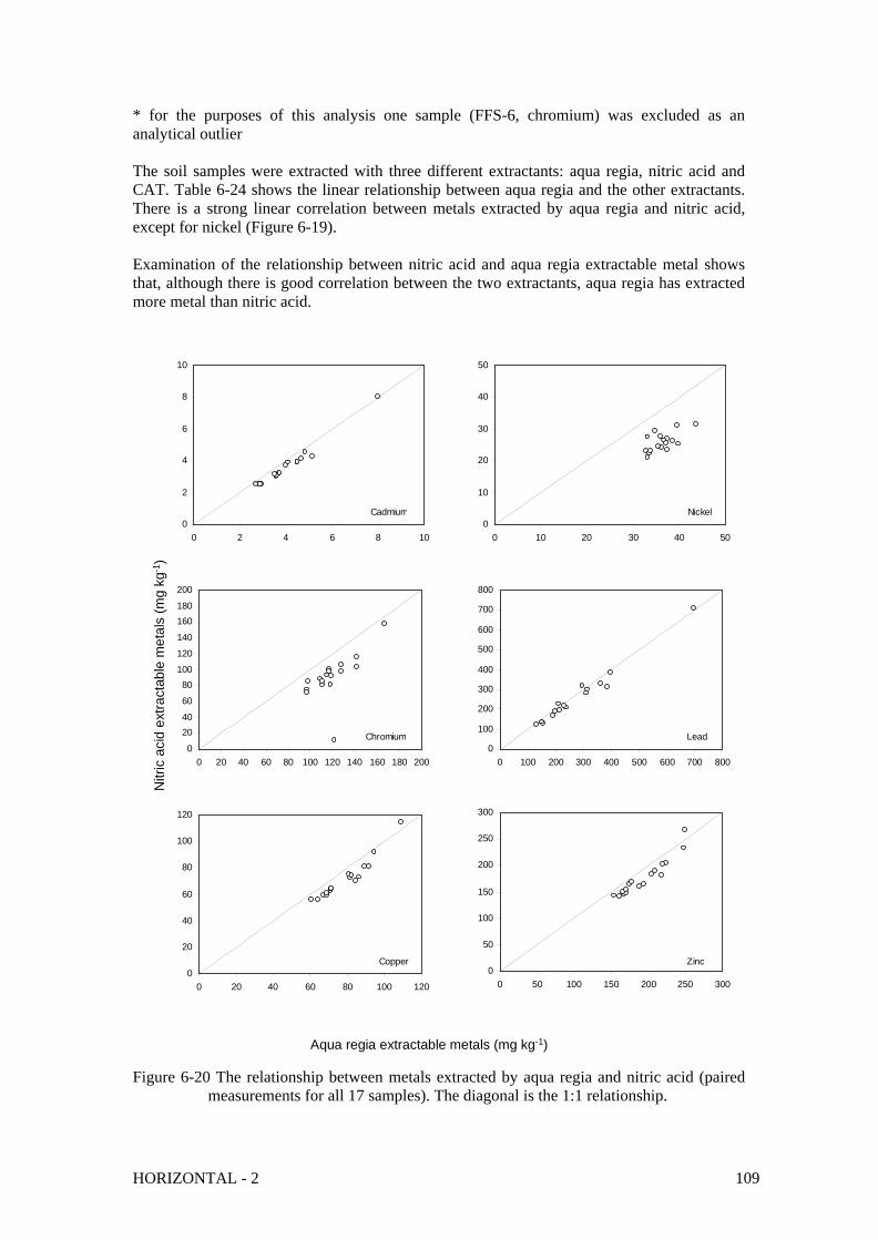
HORIZONTAL - 2 109

* for the purposes of this analysis one sample (FFS-6, chromium) was excluded as an analytical outlier The soil samples were extracted with three different extractants: aqua regia, nitric acid and CAT. Table 6-24 shows the linear relationship between aqua regia and the other extractants. There is a strong linear correlation between metals extracted by aqua regia and nitric acid, except for nickel (Figure 6-19). Examination of the relationship between nitric acid and aqua regia extractable metal shows that, although there is good correlation between the two extractants, aqua regia has extracted more metal than nitric acid.

0

2

4

6

8

10

0 2 4 6 8 10

Cadmium0

10

20

30

40

50

0 10 20 30 40 50

Nickel

0

20

40

60

80

100

120

140

160

180

200

0 20 40 60 80 100 120 140 160 180 200

Chromium0

100

200

300

400

500

600

700

800

0 100 200 300 400 500 600 700 800

Lead

0

20

40

60

80

100

120

0 20 40 60 80 100 120

Copper0

50

100

150

200

250

300

0 50 100 150 200 250 300

Zinc


Nitr

ic a

cid

extr

acta

ble

met

als

(mg

kg-1

)

Figure 6-20 The relationship between metals extracted by aqua regia and nitric acid (paired

measurements for all 17 samples). The diagonal is the 1:1 relationship.

6.5.2.4 Plant uptake

The uptake of metals by grain was low. A comparison of grain metals with typical metal concentrations for wheat is shown in Table 6-25. In the case of Cr, Cu, Pb and Zn all the grain samples were within the normal range. For cadmium three samples were outside the range and for nickel six sample exceeded the range, however it should be noted that crop was immature (8 weeks before harvest) and metals in the grain would reduce due to additional carbohydrate (photosynthate). Table 6-25 Comparison of immature grain metal with typical values for wheat. Cd Cr Cu Ni Pb Zn mg kg-1 DS Typical range*

0.012-0.26 0.014-0.2 0.6-10 0.17-0.7 0.1-1.0 16-67

This work 0.06-0.36 0.02-0.14 4.46-6.07 0.22-1.29 0.03-0.06 30.7-52.9 * Data for mature grains from Kabata-Pendias and Pendias, 2000 The metal content of the soil was above the permissible limits but the metal content of the grain was within the normal range. There was no sign of disease in the plants and the crop development appeared uniform over the sampling area. This indicates that the soil metal content was not sufficiently high to significantly affect the yield or the health of the plants (although neither effect was tested in this work). Table 6-26 shows the relationship between the amount of metal extracted and the amount of metal in the grain. Aqua regia and nitric acid extraction of soil perform poorly as predictors of grain metal concentrations. CAT extraction also performs poorly for grain Cr, Cu and Pb, but is a much better predictor of grain Cd, Ni and Zn. Table 6-27 shows the relationship between plant metal content and pH despite the variation of pH from 6.1 to 8.0 (water) [5.6 to 7.4 CaCl2] the trace element concentration in the immature grain only showed a relation with pH for Ni..

6.5.3 Conclusions Geostatistical analysis of an arable and a pasture field studied by Powlesland and Ellis (1986) produced robust variograms which suggested an optimum distance of 28m for the arable field and 34m for the pasture field. The sampling distance used in the survey of Frogmore Farm (24m) was within the sampling distances identified in the earlier work. Annex IIC of the ‘Sludge Directive’ (CEC, 1986) states that for soil sampling ‘The representative soil samples for analysis should normally be made by mixing together 25 core samples taken over an area not exceeding 5 hectares which is farmed for the same purpose. The samples must be taken to a depth of 25cm unless the depth of the surface soil is less that that value: however the sampling depth in the latter case must not be less than 10cm’. In this work the test designs comprised nine samples within an area of 0.9ha and results in a bias of up to 23.3% of the estimate of the mean. The number of samples used in this experimental work was small. Powlesland and Ellis (1986) used many more samples, the area surveyed was of a similar size. It is possible that the conclusions would have been different if more samples had been collected over a larger area, say 4 ha.

HORIZONTAL - 2 111

None of the sampling patterns performed better than any other, but the experimental work needs to be refined and to include more intensive sampling. Aqua regia extracted more metal than nitric acid, but there was a strong correlation between the measurements. The comparison was based on results from 17 samples of a soil from one field. It may not be possible to transfer these conclusions to other fields, where the soil characteristics are different, for example with respect to organic matter content, pH, and clay content. The concentrations of all of the trace elements were considerably increased above background as was expected from the historic use of sewage sludge that was produced before source control of pollutants from industry had been effective. The concentrations were also spatially heterogeneous reflecting the old method of application using rigid sectional irrigation pipes that were repositioned periodically. Although the soil samples were above the limits set for most metals, the grain metal content was within the limits of normal. None of the soil extractants performed well in the prediction of grain metal content. CAT was better than aqua regia and nitric acid for predicting grain Cd, Ni and Zn. The grain was not fully ripened, which may have affected the results.

Table 6-26 The relationship between metal content of grain and soil: Linear regression factors Aqua regia extractable Nitric acid extractable

CAT extractable

slope intercept R2 slope intercept R2 slope intercept R2

Cd 0.049 -0.40 0.37 0.046 -0.007 0.35 0.095 -0.038 0.54 Cr 0.0003 0.035 0.02 0.0004 0.029 0.14 -0.261 0.078 0.04 Cu -0.001 5.421 0.001 -0.003 5.373 0.011 -0.006 5.303 0.015 Ni 0.034 1.818 0.06 -0.054 1.976 0.17 0.181 0.088 0.78 Pb 0.00003 0.035 0.21 0.00003 0.035 0.20 0.00004 0.039 0.06 Zn 0.122 14.63 0.27 0.103 19.95 0.26 0.267 23.96 0.58

Table 6-27 The relationship between metal content of grain and soil pH: Linear regression factors pH (water) slope intercept R2 Cd -0.09 0.80 0.36 Cr 0.02 -0.04 0.11 Cu 0.02 4.97 0.0009 Ni -0.54 4.46 0.89 Pb -0.01 0.10 0.24 Zn -9.17 104.11 0.24

113

REFERENCES

Aichberger, A., Eibelhuber, A. and Hofer, G. 1986. Soil sampling for trace element analysis and its statistical evaluation. In: Sampling problems for the chemical analysis of sludge, soils and plants. A. Gomez, R. Leischber and P. L’Hermite (eds). Elsevier Applied Science, London. pp 38-44. Andronikov, S.V., Davidson, D.A. and Spiers, R.B., 2000. Variability in contamination by heavy metals: Sampling implications. Water Air and Soil Pollution, 120, 29-45. Argyraki, A., Ramsey, M.H. and Thompson, M., 1995. Proficiency testing in sampling: Pilot study on contaminated land. Analyst, 120, 2799-2803. Brus, D.J., Spatjens, L.E.E.M., de Gruijter, J.J., 1999. A sampling scheme for estimating the mean extractable phosphorus concentration of fields for environmental regulation. Geoderma, 89, 129-148. CEC (1986) Commission of the European Communities (1986) Council Directive of 12 June 1986 on the protection of the environment, and in particular of the soil, when sewage sludge is used in agriculture (86/278/EEC). Official Journal of the European Communities, No L181/6 12. de Zorzi, P., Belli, M., Barbizzi, S., Menegon, S. and Deluisa, A., 2002. A practical approach to assessment of sampling uncertainty. Accreditation & Quality Assurance, 7, 182-188. Donohue, S.J., 2002. Evaluation of soil nutrient variability for development of turfgrass soil test sampling methods. Communications in Soil Science and Plant Analysis, 33, 3335-3345. EC (2002) Regulation (EC) No 1774/2002 of the European Parliament and of the Council of 3 October 2002 laying down health rules concerning animal by-products not intended for human consumption. Official Journal of the European Communities L 273/1 10.10.2002 http://europa.eu.int/comm/food/fs/bse/legislation_en.html#by-products Frogbrook, Z.L. and Oliver, M.A., 2001. Comparing the spatial predictions of soil organic matter determined by two laboratory methods. Soil Use and Management, 19, 235-244. Frogbrook, Z.L., Oliver, M.A., Salahi, M. and Ellis, R.H., 2002. Exploring the spatial relations between cereal yield and soil chemical properties and the implications for sampling. Soil Use and Management, 18, 1-9. Gomez, A., Leschber, R. and Colin, F., 1986. Sampling techniques for sludge, soil and plants. In: Sampling problems for the chemical analysis of sludge, soils and plants. A. Gomez, R. Leischber and P. L’Hermite (eds). Elsevier Applied Science, London. pp 80-90. Jarvis R.A., 1968 Soils of the Reading District. Memoir of the Soil Survey of Great Britain Bulletin No.8, Harpenden Kabat-Pendias, A. and Pendias, H., 2000. Trace elements in soils and plants, 3rd edition, CRC Press, Bocca Raton, Fla. Laraia, R., Cortellini, L., De Poli, F., 2002. Sampling protocols for ensuring legal compliance and standardisation: the case of Italy. Biodegradable treatment of biodegradable waste, Bruxelles, 8-10 April 2002. Lee, J-C and Ramsey, M.H., 2001. Modelling measurement uncertainty as a function of concentration: an example from a contaminated land investigation. Analyst, 126, 1784-1791. Lock, W.H., 1996. Composite sampling. National Environmental Health Forum Monographs. Soil Series; no. 3. Department of Human Services, Australia. Payne, R. W. 1993. Genstat 5 Release 3 Reference Manual Planned and written by the GENSTAT 5 COMMITTEE, AFRC Institute of Arable Crops Research, Harpenden, Herfordshire. Oxford University Press Powlesland, C. and Ellis, J.C., 1986. Sampling procedures for sludge treated soils (SDD 9313 SLD). Final report to the Department of the Environment. WRc Environment, Marlow, UK. Ramsey, M.H. and Argyraki, A., 1997. Estimation of measurement uncertainty from field sampling: implications for the classification of contaminated land. The Science of the Total

114

Environment, 198, 243-257. Ramsey, M.H., Argyraki, A. and Thompson, M., 1995. Estimation of sampling bias between different sampling protocols on contaminated land. Analyst, 120, 1353-2803. Squire, S., Ramsey, M.H. and Gardner, M.J., 2000. Collaborative trial in sampling for the spatial delineation of contamination and the estimation of uncertainty. Analyst, 125, 139-145. TMECC, 2001. Sample collection and laboratory preparation: Field sampling of compost materials. Chapter 2 in: Test Methods for Examination of Composting and Compost, TMECC Manual. http://tmecc.org/tmecc/Table_of_Contents.html#01 Wagner, G., Mohr, M.-E., Strengart, J., Desaules, A., Muntau, H., Theocharopoulos, S. and Quevauviller, P., 2001. Objectives, concept and design of the CEEM soil project. The Science of the Total Environment, 264, 3-15. Wang, X.J. and Qi, F., 1998. The effects of sampling design on spatial structure analysis of contaminated soil. The Science of the Total Environment, 224, 29-41. Watanabe, Y. and Tanaka, K., 1999. Innovative sludge handling through pelletization/thickening. Water Research, 33, 3245-3252. Webster, R and Oliver, M.A., 2001. Geostatistics for environmental scientists. John Wiley and Sons, Chichester, UK.

115

1 APPENDIX 1 - PERRY OAKS SLUDGE DEWATERING WORKS

1.1 Site description

Mogden sewage treatment works (STW) and Perry Oaks sludge dewatering plant serve a population of some 1.8 million residing within a catchment area covering north-west and west London. Mogden STW produces approximately 75tDS/day digested sludge, which is pumped to Perry Oaks (11.5 km to the west) for dewatering. The processed solid component is ultimately recycled to land, the liquid effluent being returned to Mogden for treatment. The liquid sludge is delivered to one of six large holding tanks where it is mixed by aeration then passed to one of four large Alfa Laval Sharples PM9100 dewatering centrifuges. The dewatering process increases the dry solids (DS) content from about 4% DS in the sludge to about 25-30% DS in the cake. Over a period of 24 hours approximately 40 tonnes of cake are produced from a single centrifuge. The cake is passed from the centrifuge via a screw conveyor to a drop zone, where it builds into conical piles of dewatered cake. The piles are cleared twice each day to stockpiles approximately 2.5m high on concrete storage areas. After a minimum period of two weeks to allow for stabilisation, the sludge cake is delivered to farmland. It is transported in sheeted lorries and applied to the farmland using specialist low ground pressure precision spreaders designed to minimise damage to soil structure. Access to fields could be disrupted because of weather conditions. In this case it may be stockpiled on farms rather than applied immediately. Demand for cake varies, being at its lowest between May and early July, and at its highest, following the harvest, between mid July and November. During periods of low demand the cake is stockpiled at Perry Oaks or on farms awaiting periods of greater demand.

1.2 Sampling: Standard Operating Procedures

The surface layers are subject to rain, leaching and environmental contamination. These layers (at least 100 mm) are removed before sampling, so that the crust does not become part of the sample. It is not practical or safe to walk over the top of a stockpile to collect samples, so the latest addition to the stockpile is regarded as representative of the period of cake production since the last sampling. A mechanical digger is used to remove cake from the side wall of the stockpile and samples are taken randomly from the exposed face. Five samples (each at least 100 g) are collected and examined separately for the microbiological parameters. A composite sample is made for analysis of dry solids, LOI, metals and nutrients.

1.3 Experimental sampling plan

A sampling plan was drawn up to answer the following questions: • Does the point at which the samples are taken affect the results?

- Sample the liquid feed to a centrifuge at time intervals - Sample the dewatered cake produced by the same centrifuge at the same time

intervals - Sample around the pile of cake produced over the sampling period - Sample inside the pile of cake produced over the sampling period

• When sampling the pile, does it matter what sampling device is used?

116

- Sample the cake pile using a trowel - Sample the cake pile at the same location using a core sampler

• When sampling around the pile, does it matter at what depth the pile is sampled?

- Sample the cake pile using a core sampler at 0-25 cm - Sample the cake pile using a core sampler at 25-50 cm

• When sampling the pile, does it matter how many samples are taken?

- Sample around the pile taking many samples • How do the results compare to coning and quartering the pile? To answer these questions digested sludge was sampled at several stages in the process (Figure 1-1):

a. The liquid sludge feed to a centrifuge and dewatered cake produced by the same centrifuge (9 samples at 40 minute intervals)

b. Around the pile created during (a) using different sampling devices (7 samples taken with a trowel and a core sampler)

c. Around the perimeter of the pile created during (a) at 2 different depths into the pile (7 samples taken at 0-25 cm and 25-50 cm with a core sampler)

d. Halve the pile using a loading shovel and sample across the exposed face (12 samples taken with a trowel)

e. Cone and quarter the pile mechanically with a loading shovel then manually cone and quarter the remainder (4 samples)

1.4 Sample collection

The drop zone was cleared of cake that had accumulated overnight to the stockpile area before sampling began. Liquid digested sludge samples were collected from a sampling tap into a plastic screw-top bottle and labled. Before filling the bottle was rinsed with sludge, which was discarded. Immediately after collecting a sample of the liquid feed a sample of cake was collected from the end of the conveyor using a clean spade. Cake samples were transferred to polythene bags, sealed and labled. At the end of the day samples were taken from around the pile. Single samples were taken using a clean trowel or composite samples (5 cores) taken with a core sampler. Then the pile was halved using a mechanical shovel and samples were collected from the resultant face using a trowel. The pile was further halved twice mechanically and the remainder moved to a separate area for coning and quartering manually. At the end of the day the samples were checked against the sampling sheet and transferred to a cold room (4oC) to await analysis.

1.5 Observations made during sampling

For several days prior to sampling the weather had been changeable with showers. On the day of sampling the weather was variable, mostly dry and overcast with occasional light showers during the first half of the day and sunshine later. Three of the four centrifuges were in operation. There was variation in the efficiency of the centrifuges, which resulted in variation in the physical characteristics of the cake. The cake falling from the end of the conveyors varied from small (<5 cm) to large lumps (>15 cm) reflecting differences in the water content of the cake.

117

As the smaller lumps fell onto the top of the pile they tended to roll down the sides forming a cone-shaped pile. When the larger lumps fell onto the top of the pile they remained at the top of the pile, which appeared to compact on impact. Eventually, after several large lumps had fallen, the pile changed shape being a cone at the base with a large mass resting on top. Intermediate sized lumps tended to roll to the bottom and accumulate around the base of the pile.

1.6 Sampling logistics

There was no difficulty accessing or operating the sampling tap for liquid sludge. To avoid spatter when filling a wide-necked bottle was used. Access to the end of the conveyor was via a metal mesh ramp (with grip teeth) that was protected by a safety rail. Operator safety was of greater concern when sampling from the pile in the drop zone. In order to reach the pile it was necessary to walk over a concrete surface where vehicles had been driven (mechanical shovel and trucks). Here the ground surface was very greasy and slippery. This was a combination of the nature of the cake, the weather and the vehicles. It was observed that the slippery surface occasionally presented a problem for the mechanical shovel when it was manoeuvring under load. When sampling around the outside of the pile several difficulties were encountered, some of which involved operator safety. The surface of the pile was very loose and prone to slippage as the samples were taken. As the cake fell it covered the sampler’s feet making it difficult to manoeuvre with risk of over-balancing. This meant that it was not possible to control the sampling direction into the pile and the height at which samples could be taken was limited to the reach of the sampler. Since the centrifuge was in continuous operation cake was falling onto the pile (and the sampler) during the sampling process. This compromises the safety of the sampler. Continuous vigilance was required to avoid being hit by large lumps of cake falling from the conveyor. Manual coning and quartering of the cake proved to be time consuming, difficult and heavy work. The texture of the cake was similar to a wet heavy clay soil. It had a tendency to clump together into large clods as the spade was pushed into the pile. When the cake was transferred from the spade the clods fell onto the top in a single mass instead of falling to form a cone. Attempts were made to break up the cake but with limited success. Due to time constraints, only one cone was produced manually. This was marked out into quarters using the spade and four samples were collected, one from each quarter. Note: TERRA ECO⋅SYSTEMS’ Standard Operating Procedure for sampling is to sample from the stockpile prior to cake being removed for delivery, thus avoiding the hazards experienced during this sampling exercise.

1.7 Results

The results of the analyses are shown in Table 1-1.

118

Centrifuge Pile

Conveyor

Cake

12T 6T 3T 1.5T

2

3

5

Inlet

1

Liquid

Sludge

4

Mechanical Shovel

Manual Coning and Quartering

Sampling Points

1: Liquid Sludge Inlet

2: Conveyor

3: Around Pile

4: Pile Face

5: Cone & Quarter

Figure 1-1 Perry Oaks experimental sampling plan

Table 1-1 Analytical results for Perry Oaks experimental sampling: Liquid Sludge Sample DS% LOI%(DS) Cd Cr Cu Ni Pb Zn Aqua Regia Extractable (mg kg –1 DS)

DSS-1 2.06 60.7 3.74 47.1 468 34.3 136 704 DSS-2 2.07 62.3 3.53 42.9 391 27.0 124 493 DSS-3 2.16 63.4 3.15 45.7 372 28.0 118 477 DSS-4 2.07 63.8 4.48 47.4 403 28.8 135 512 DSS-5 2.23 64.6 2.87 53.8 367 31.8 115 462 DSS-6 2.00 63.0 3.55 47.3 419 30.4 130 585 DSS-7 2.15 64.2 4.09 49.8 400 30.6 126 512 DSS-8 2.14 64.0 3.08 46.2 407 29.2 126 491 DSS-9 2.12 65.1 3.07 46.3 407 31.5 132 505 Nitric Acid-Extractable(mg kg –1 DS)

DSS-1 3.69 36.7 438 29.5 134 592 DSS-2 3.14 40.2 441 27.8 174 517 DSS-3 3.19 46.8 420 31.6 137 528 DSS-4 3.24 42.1 440 33.0 137 522 DSS-5 3.14 65.5 404 31.5 134 489 DSS-6 1.55 106.0 469 40.7 175 600 DSS-7 3.30 37.4 433 26.8 142 488 DSS-8 3.32 55.1 438 30.0 136 514 DSS-9 3.25 46.4 428 29.7 146 491 CAT-Extractable(mg kg –1 DS)

DSS-1 <0.05 <0.05 3.40 7.77 35.9 28.6 DSS-2 <0.05 <0.05 4.35 9.18 44.0 21.7 DSS-3 <0.05 <0.05 2.78 7.41 29.6 14.8 DSS-4 <0.05 <0.05 2.90 6.76 26.6 12.1 DSS-5 <0.05 <0.05 3.14 5.83 22.4 12.6 DSS-6 <0.05 <0.05 3.50 5.00 14.0 8.5 DSS-7 <0.05 <0.05 3.26 5.58 18.1 9.8 DSS-8 <0.05 <0.05 3.27 7.01 26.2 13.1 DSS-9 <0.05 <0.05 2.36 5.66 18.4 9.9

120

Table 1-2 Analytical results for Perry Oaks experimental sampling: Dewatered cake Sample DS% LOI%(DS) Cd Cr Cu Ni Pb Zn Aqua Regia-Extractable (mg kg –1 DS)

Conveyor DWC-1 21.1 64.4 3.94 42.8 400 29.6 133 490 DWC-2 21.8 64.6 3.78 43.2 397 29.9 133 488 DWC-3 21.5 65.1 3.91 45.8 404 30.5 136 500 DWC-4 21.6 65.1 3.86 42.6 399 30.5 137 497 DWC-5 21.5 65.2 3.76 48.2 405 31.7 133 497 DWC-6 22.1 65.3 3.92 41.1 396 28.6 134 492 DWC-7 22.1 65.6 3.76 46.0 395 29.5 135 492 DWC-8 22.0 65.5 3.80 43.3 389 29.0 132 482 DWC-9 22.0 65.5 3.60 46.2 381 30.0 132 475 Trowel around pile DWC-10 22.0 65.2 4.39 50.9 440 33.5 150 546 DWC-11 22.2 65.2 3.91 43.2 410 18.0 138 511 DWC-12 21.9 65.1 4.05 45.4 409 17.6 139 516 DWC-13 22.3 65.5 3.91 47.6 416 19.3 140 524 DWC-14 22.3 65.2 3.88 46.4 401 18.4 136 512 DWC-15 22.0 65.4 3.94 47.5 404 18.7 140 511 DWC-16 21.9 65.3 3.98 47.1 416 17.9 140 520 DWC-17 21.6 64.9 3.88 46.4 413 17.6 139 511 DWC-18 22.1 65.4 3.74 46.8 406 17.3 142 507 DWC-19 22.0 65.5 3.83 46.9 407 17.8 142 515 DWC-20 22.2 65.3 3.96 48.2 408 18.8 138 512 DWC-21 22.0 65.0 3.96 47.9 413 22.1 144 517 DWC-22 22.1 65.1 3.82 43.7 414 17.4 140 511 DWC-23 22.3 65.3 3.98 46.0 416 19.3 140 518 DWC-24 22.0 64.8 3.83 49.4 404 17.6 140 514 DWC-25 22.1 65.5 3.73 46.0 401 17.8 137 501 DWC-26 22.2 65.4 3.81 46.9 415 17.8 135 514 DWC-27 22.2 65.2 3.88 47.1 412 17.9 141 511 DWC-28 21.9 65.2 3.81 47.4 404 16.9 136 505 DWC-29 22.3 65.2 3.80 47.8 403 18.0 139 504 DWC-30 22.1 65.0 4.09 44.0 414 17.9 138 509 DWC-31 22.4 64.9 3.85 38.3 405 19.0 138 501 Corer: 0-25 cm DWC-32 24.1 59.6 4.07 45.0 407 18.5 140 523 DWC-33 22.0 65.0 4.00 44.9 415 18.9 139 520 DWC-34 22.0 65.2 4.12 46.3 420 18.6 144 531 DWC-35 21.8 65.1 4.04 47.0 414 19.2 140 522 DWC-36 21.8 64.5 4.40 47.4 425 18.5 144 533 DWC-37 21.9 64.8 3.96 46.5 414 18.2 137 514 DWC-38 22.3 64.9 4.05 48.2 410 18.5 137 507 Corer: 25-50 cm DWC-39 21.9 64.8 4.11 48.5 411 18.1 141 520 DWC-40 22.0 64.7 4.00 48.0 411 18.1 136 517 DWC-41 22.0 65.2 4.05 48.6 417 18.6 142 527 DWC-42 21.8 65.2 3.93 47.1 418 18.1 139 528 DWC-43 21.9 65.1 3.93 49.3 417 18.9 140 525 DWC-44 22.0 65.2 3.91 50.3 424 19.4 142 525 DWC-45 22.1 65.2 4.00 48.6 429 19.9 142 534

Sample DS% LOI%(DS) Cd Cr Cu Ni Pb Zn Face DWC-46 22.3 65.3 3.84 46.3 398 17.6 137 494 DWC-47 22.0 65.1 4.03 46.6 412 18.0 140 516 DWC-48 21.7 65.0 3.87 54.7 404 20.9 137 497 DWC-49 21.8 64.8 4.01 49.9 422 18.2 144 519 DWC-50 22.0 65.1 4.40 49.7 422 18.2 143 521 DWC-51 22.0 65.3 3.78 47.8 409 18.2 137 498 DWC-52 22.3 65.6 4.19 47.4 417 18.3 137 507 DWC-53 21.9 65.7 3.95 47.2 414 18.1 144 512 DWC-54 22.2 65.3 3.91 46.8 416 18.3 146 515 DWC-55 22.0 65.6 3.91 46.1 415 18.5 140 519 DWC-56 21.9 65.4 4.04 49.5 419 18.3 145 515 DWC-57 21.8 65.3 4.05 43.4 412 18.4 138 511 Cone and quarter DWC-58 22.3 65.3 4.14 46.4 415 17.2 140 517 DWC-59 22.2 65.5 3.95 49.8 418 17.7 142 511 DWC-60 22.1 65.4 4.08 47.6 416 18.1 142 514 DWC-61 22.3 64.9 4.24 46.8 398 32.9 152 491

122

Table 1-2 (continued). Analytical results for Perry Oaks experimental sampling: Dewatered cake Sample Cd Cr Cu Ni Pb Zn

Nitric Acid -Extractable (mg kg –1 DS)

Conveyor DWC-1 3.68 40.4 410 30.6 139 498 DWC-2 3.77 39.1 409 28.5 137 502 DWC-3 3.61 38.1 403 28.4 136 490 DWC-4 3.70 38.9 406 29.0 140 495 DWC-5 3.85 38.9 411 29.2 141 504 DWC-6 3.60 37.9 406 28.2 138 489 DWC-7 3.81 39.4 402 29.3 141 492 DWC-8 3.71 38.5 410 28.6 138 500 DWC-9 3.85 3.85 398 28.5 137 486 Trowel around pile DWC-10 3.80 38.1 405 28.5 135 492 DWC-11 3.79 40.2 405 29.2 136 502 DWC-12 3.81 38.6 406 29.0 138 493 DWC-13 3.72 38.9 405 31.7 138 489 DWC-14 3.60 38.7 397 29.0 139 489 DWC-15 3.74 38.8 411 29.6 137 499 DWC-16 3.89 39.1 410 28.9 138 497 DWC-17 4.19 39.5 410 29.2 138 493 DWC-18 3.80 40.0 403 28.1 135 493 DWC-19 3.76 38.3 403 28.9 137 495 DWC-20 3.62 39.4 407 29.0 142 490 DWC-21 6.82 40.7 414 30.5 142 501 DWC-22 3.80 37.0 394 28.2 134 478 DWC-23 3.98 38.8 402 28.8 139 494 DWC-24 3.68 39.9 398 28.2 140 492 DWC-25 3.60 38.6 396 28.2 135 481 DWC-26 3.76 38.7 406 28.6 143 505 DWC-27 3.66 39.1 406 28.7 138 495 DWC-28 3.73 39.3 417 29.1 142 503 DWC-29 3.65 38.7 401 28.7 136 492 DWC-30 4.17 37.6 402 28.7 134 488 DWC-31 3.72 36.1 390 28.1 129 477 Corer: 0-25 cm DWC-32 4.56 37.2 397 28.1 131 497 DWC-33 3.59 36.2 390 27.5 127 477 DWC-34 3.61 36.4 387 28.1 130 482 DWC-35 3.79 36.6 399 27.9 135 492 DWC-36 3.56 36.4 389 27.9 131 494 DWC-37 3.67 37.8 390 28.2 130 490 DWC-38 3.67 36.4 392 27.7 131 484 Corer: 25-50 cm DWC-39 3.71 36.0 391 27.7 128 513 DWC-40 3.82 36.1 398 27.6 128 489 DWC-41 4.01 37.9 398 28.7 135 498 DWC-42 3.78 36.8 399 28.3 135 493 DWC-43 3.59 36.0 395 27.8 130 495 DWC-44 3.68 35.7 401 27.3 131 490 DWC-45 3.60 36.7 394 28.3 134 491

Sample Cd Cr Cu Ni Pb Zn

Face DWC-46 3.55 35.9 381 27.6 129 481 DWC-47 3.69 36.3 393 30.0 132 479 DWC-48 3.64 36.9 397 28.3 133 481 DWC-49 3.80 37.1 396 28.3 134 484 DWC-50 3.52 35.9 392 27.3 131 473 DWC-51 3.74 38.3 390 29.1 132 488 DWC-52 3.90 39.5 426 30.0 141 522 DWC-53 3.62 35.8 391 28.4 131 483 DWC-54 3.69 35.4 383 27.3 129 486 DWC-55 3.67 36.5 387 28.0 134 486 DWC-56 3.60 36.4 402 28.6 133 494 DWC-57 3.58 35.8 390 28.8 130 484 Cone and quarter DWC-58 3.72 35.5 387 27.3 130 478 DWC-59 3.66 36.4 388 28.0 131 489 DWC-60 3.56 34.6 387 28.5 126 480 DWC-61 3.56 37.4 392 28.6 134 483

124

Table 1-2 (continued). Analytical results for Perry Oaks experimental sampling: Dewatered cake Sample Cd Cr Cu Ni Pb Zn

CAT -Extractable (mg kg –1 DS)

Conveyor DWC-1 0.12 <0.05 11.1 3.89 12.1 28.9 DWC-2 0.14 <0.05 13.3 4.79 13.7 33.9 DWC-3 0.12 <0.05 12.5 3.86 13.8 28.4 DWC-4 0.12 <0.05 12.6 4.03 13.4 28.9 DWC-5 0.14 <0.05 12.9 5.06 11.4 33.5 DWC-6 0.10 <0.05 12.6 3.23 11.0 23.4 DWC-7 0.11 <0.05 14.9 3.89 12.3 26.9 DWC-8 0.12 <0.05 14.6 3.90 9.9 26.4 DWC-9 0.13 <0.05 13.9 4.49 8.5 27.9 Trowel around pile DWC-10 0.14 <0.05 14.8 4.44 9.2 27.5 DWC-11 0.12 <0.05 17.5 3.81 11.6 26.1 DWC-12 0.15 <0.05 16.8 4.48 11.8 34.8 DWC-13 0.12 <0.05 11.2 4.07 6.9 26.0 DWC-14 0.12 <0.05 12.0 4.05 7.3 25.8 DWC-15 0.13 <0.05 12.7 4.24 8.3 27.3 DWC-16 0.14 <0.05 16.8 4.52 12.5 33.4 DWC-17 0.15 <0.05 14.3 4.53 12.4 32.1 DWC-18 0.15 <0.05 11.8 4.97 13.3 35.1 DWC-19 0.14 <0.05 9.2 5.08 10.3 33.0 DWC-20 0.14 <0.05 11.1 4.56 12.7 33.4 DWC-21 0.17 <0.05 13.5 4.86 13.9 42.5 DWC-22 0.19 <0.05 12.3 6.26 15.7 48.1 DWC-23 0.18 <0.05 10.8 6.33 13.6 41.0 DWC-24 0.20 <0.05 10.2 6.54 17.0 48.2 DWC-25 0.19 <0.05 9.9 6.54 14.9 42.6 DWC-26 0.19 <0.05 11.7 5.01 22.5 45.6 DWC-27 0.26 0.05 10.8 6.66 19.1 62.6 DWC-28 0.23 <0.05 11.5 6.29 22.4 56.7 DWC-29 0.23 <0.05 14.6 5.77 23.0 53.5 DWC-30 0.24 <0.05 15.4 6.33 23.8 57.7 DWC-31 0.20 <0.05 13.2 5.32 15.6 40.3 Corer: 0-25 cm DWC-32 0.22 <0.05 9.2 7.00 12.1 43.4 DWC-33 0.22 <0.05 10.2 6.78 12.4 40.6 DWC-34 0.20 <0.05 11.2 6.51 13.7 40.1 DWC-35 0.23 <0.05 12.6 6.08 17.4 44.7 DWC-36 0.22 <0.05 12.9 6.35 16.3 43.0 DWC-37 0.19 <0.05 10.2 5.21 18.3 39.6 DWC-38 0.23 <0.05 11.1 6.24 13.0 43.6 Corer: 25-50 cm DWC-39 0.21 <0.05 11.9 5.92 15.9 41.5 DWC-40 0.21 <0.05 12.0 5.25 17.8 38.8 DWC-41 0.22 <0.05 12.2 6.47 16.0 45.1 DWC-42 0.20 <0.05 14.3 5.27 18.9 39.6 DWC-43 0.22 <0.05 14.2 6.12 17.7 46.2 DWC-44 0.22 <0.05 15.0 5.16 17.5 38.5 DWC-45 0.20 <0.05 11.8 5.96 13.8 39.3


Face DWC-46 0.19 <0.05 11.5 5.94 14.8 39.9 DWC-47 0.18 <0.05 13.3 4.73 16.8 34.9 DWC-48 0.19 <0.05 13.0 5.03 17.4 38.3 DWC-49 0.19 <0.05 15.7 4.64 14.9 34.0 DWC-50 0.19 <0.05 11.9 4.85 14.8 34.6 DWC-51 0.19 <0.05 12.6 4.63 15.1 33.7 DWC-52 0.21 <0.05 11.8 5.45 14.9 38.6 DWC-53 0.18 <0.05 10.9 4.36 14.5 32.2 DWC-54 0.19 <0.05 12.0 4.71 14.0 35.2 DWC-55 0.16 <0.05 11.9 3.91 15.4 31.3 DWC-56 0.18 <0.05 12.1 4.65 18.0 35.7 DWC-57 0.17 <0.05 13.1 4.55 17.0 37.8 Cone and quarter DWC-58 0.16 <0.05 9.9 4.64 14.6 33.6 DWC-59 0.13 <0.05 11.4 3.11 11.7 25.5 DWC-60 0.14 <0.05 10.8 3.46 14.0 25.4 DWC-61 0.19 <0.05 14.3 5.17 16.9 36.5

126

2 APPENDIX 2 BUDDS FARM


Budds Farm recycling centre has been in operation since 1953 and has the capacity to process 20,000 tonnes dry solids per year. The drier was commissioned in 2002. The centre currently processes sludges equivalent to a population of 600,000. The feedstocks are: - Sludge from the on-site wastewater treatment works; - Sludge from other wastewater treatment works; - Cake transferred from other wastewater treatment works within the water company area. Feedstock to the treatment works is wastewater from the local Havant area and wastewater transferred from Portsmouth via a 7.8 km tunnel. The wastewater undergoes four stages of treatment; screening, grit removal, primary and secondary biological treatment. Following a period in the final settlement tanks, the cleaned wastewater is sent back to Portsmouth via the tunnel and released 5 km out to sea at Eastney via a pumping station. The sludge is transferred to the recycling works. The first stage of the recycling process involves blending the sludge from the different sources in varying proportions. The sludge is then and thickened to approximately 7% DS and fed into one of the anaerobic digesters (capacity of each tank 2750 m3) where it undergoes digestion at 35oC. In the digestion process organic matter is broken down creating water and biogas. The biogas gas is stored on-site in a gas holder before being recycled back into the works to provide heat and power for the treatment process. After an average period of 14 days approximately 40% of the total organic material has been destroyed and the sludge is approximately 4.5% DS. The digested material is removed to storage tanks. Following storage the liquid sludge is dewatered by centrifuge to create a cake, average 25% DS. The cake is passed to the thermal drying process. The dewatered sludge is fed into a mixer, where it is mixed with ‘base material’, a mix of crushed oversize granules and undersize granules that are fed back into the system. This produces material that is no longer sticky and also creates a moist granule mixture. This mixture is brought to the drum inlet and dried to at least 90% DS by hot air in the triple pass, rotating drum. The material is cooled then screened. The coarser product (>4 mm) is passed through a crusher and returned to the mixer for use as backfeed material along with the finer product (<2 mm). Granules 2-4 mm pass into a storage silo to await bagging. Typically bagging takes place three times a day, when the storage silos are reaching capacity. The granules are fed into strong plastic bags that are contained inside woven plastic sacks. During the filling process the plastic liner is sealed around the feed pipe and an extractor fan is switched on to minimise dust levels. Once full, the inner bag is sealed and the outer sack is labelled with the date of production and a bag number. In total 30-40 1000 kg bags are produced each day and stored on-site before delivery to customers.

At all stages in the process measures are in place to control odour and dust. The only access to the material is via sampling taps and a granule sampler and these are in place for process control monitoring.


The production process is closed and the number of sampling locations is limited to where they have been designed in to the system. Sludge samples are taken at several points along the process for plant operational purposes. Granules are sampled for moisture analysis for process control. For regulatory parameters and nutrient analysis samples of the bagged product are collected twice per month. This is more frequently than required by legislation, but is done for internal production control and marketing requirements. Samples are collected after the bagging process. Sampling method development had been carried out at the plant and it was found that sampling at this stage minimises the risk of cross contamination from other parts of the production process. Microbiological cross contamination is the main concern (e.g. E. coli and Salmonella) rather than heavy metals. A bag is selected at random from the production process and isolated, along with the bag before and the bag after. Five samples are collected from near the top of the bag using a beaker. Clean gloves and a clean beaker are used for each sample. All five samples are examined separately for E. coli and Salmonella (This is ‘verification’ testing in this HACCP operated plant, see Appendix E). All samples must pass this test. One of the five samples is selected at random and analysed for other regulatory parameters and for nutrient content. If any sample fails the tests, the bag before and after the one selected are analysed to help identify the cause of the failure. If the samples pass the tests, then the bags they came from are returned to the production line.


A sampling plan was drawn up to answer the following questions: • Does it matter where in a bag the samples are taken? - Take samples from a single depth within the bag - Take samples from other depths within the bag • How do samples vary over time? - Take samples from the hopper feed at time intervals To answer these questions dried sludge granules were sampled at two stages in the process. a. Five samples from a single bag at one depth b. Three samples from two more depths within the same bag c. Nine samples from the hopper feed sampling point at 35 minute intervals

128

TOP OF BAG

1

4

5

8

9

2

6

10

3

7

11

BOTTOM OF BAG

Figure 2-1 Sampling scheme for a bag of granules The numbers correspond to the sample numbers in Table 2-1.

2.4 Sample Collection

A single bag was selected at random by the site manager. The bag was approximately 1.3 m high. A spade was used to remove layers of granules form the bag such that samples could be taken from depths of 250, 650 and 1050 mm. Five samples were taken from the first depth and three samples from each of the other depths. Samples were taken from within the bag with a 500 ml plastic scoop. Each sample scoop was sub-sampled by pouring the granules into a 250 ml plastic beaker, to give a final sample weight of approximately 200 g as required by the analytical laboratory. During the sampling period nine samples were collected from the granule production stream. Access was gained via a sampling scoop installed in the granule production area for production monitoring of granule moisture content. The scoop fills randomly up to 20 minutes after emptying. Samples were collected at intervals of 35 minutes. In practice, due to the random filling, this meant an actual sampling interval between 15 and 35 minutes. The samples were transferred to zip-seal polythene bags, labelled and placed in a cool box. At the end of the day the samples were checked against the sampling sheet and transferred to a cold room (4oC) to await analysis.


On the day of sampling the weather was sunny, cloudless and 26-28oC. There was a light breeze, which caused dust to rise. The dust was caused by the abrasion of the granules.


There was no difficulty accessing from the bag or the sampling point. Plant (lorries being loaded) was moving in the vicinity of the sampling. The sampling bag was in a part of the stockpile area where plant movement was minimal, to minimise the risk. The stockpile area was concrete with a thin gravel layer to maximise traction. Since the dust is a hazard, precautions were taken to avoid inhalation or abrasion of eyes and skin: eye protection, face mask and gloves.

2.7 Results

The results are shown in Table 2-1.

130

Table 2-1 Analytical results for samples collected from the bag of granules BFB-1 BFB-2 BFB-3 BFB-4 BFB-5 BFB-6 BFB-7 BFB-8 BFB-9 BFB-10 BFB-11 Mean s.d DM% 91.9 92.0 91.8 91.9 91.8 91.8 91.8 91.6 91.6 91.5 91.1 91.71 0.25 LOI% 66.7 66.9 66.9 67.2 67.0 67.6 66.8 67.1 67.1 67.2 67.4 67.08 0.26 Aqua Regia Extractable (mg kg-1 DS) Cd 1.59 1.64 1.52 1.60 1.52 1.54 1.66 1.51 1.52 1.54 1.73 1.58 0.07 Cr 37.2 36.7 36.8 36.2 36.0 38.1 40.0 37.0 36.7 40.0 50.1 38.62 4.05 Cu 506 505 493 499 485 485 503 495 491 517 572 504.6 24.3 Ni 15.6 15.2 14.7 15.0 14.6 15.1 16.9 15.1 15.0 15.5 27.5 16.38 3.74 Pb 105 106 105 102 102 106 105 102 101 107 125 106.0 6.6 Zn 497 491 483 488 468 488 491 481 484 507 550 493.5 21.1 50% Nitric Acid Extractable (mg kg-1 DS) Cd 1.35 1.37 1.34 1.36 1.37 1.36 1.41 1.37 1.37 1.33 1.46 1.37 0.04 Cr 46.1 45.7 45.3 45.4 45.6 45.2 46.9 44.9 44.8 45.5 46.7 45.65 0.68 Cu 576 568 568 575 567 567 580 574 577 572 583 573.4 5.5 Ni 24.7 24.4 24.6 25.1 25.3 24.7 24.8 25.1 25.2 24.5 25.0 24.85 0.30 Pb 124 124 116 125 119 121 122 119 119 120 122 121.0 2.7 Zn 561 549 546 555 546 549 557 552 544 552 565 552.4 6.6 CAT Extractable (mg kg-1 DS) Cd 0.28 0.28 0.28 0.28 0.26 0.24 0.25 0.26 0.25 0.26 0.24 0.26 0.02 Cr <0.05 <0.05 <0.05 <0.05 <0.05 <0.05 <0.05 <0.05 <0.05 <0.05 <0.05 <0.05 Cu 72.5 82.0 74.1 80.9 82.2 76.8 81.7 87.8 81.8 88.2 73.8 80.16 5.32 Ni 4.67 4.87 4.64 4.57 4.45 3.96 4.07 4.23 4.07 4.21 4.05 4.34 0.31 Pb 13.7 15.8 15.5 14.3 14.4 12.9 12.9 13.0 13.1 12.9 13.1 13.78 1.08 Zn 68.1 70.8 70.5 69.2 66.8 58.0 62.7 64.9 63.6 63.8 59.7 65.28 4.23

131

Table 2-2 Analytical results for time interval samples of granules collected from the in-stream sampler T1 T2 T3 T4 T5 T6 T7 T8 T9 Mean s.d DM% 91.6 91.7 92.3 92.4 92.5 92.4 92.4 92.1 91.4 92.09 0.41 LOI% 66.0 66.6 66.3 66.5 66.9 66.3 66.4 66.5 66.7 66.47 0.26 Aqua Regia Extractable (mg kg-1 DS) Cd 1.60 1.24 1.44 1.18 1.35 1.61 1.41 1.90 1.43 1.46 0.22 Cr 55.2 45.1 50.9 44.2 51.0 50.7 52.8 61.3 49.6 51.20 5.12 Cu 577 435 519 430 510 520 526 625 513 517.2 61.0 Ni 32.9 24.1 28.4 23.4 28.7 30.4 28.8 35.3 28.3 28.92 3.76 Pb 126 94.2 120 90.8 115 118 121 143 116 116.0 15.8 Zn 598 453 545 439 528 542 551 655 534 538.3 65.8 50% Nitric Acid Extractable (mg kg-1 DS) Cd 1.25 1.36 1.29 1.31 1.27 1.30 1.29 1.29 1.37 1.30 0.04 Cr 48.2 49.3 48.1 48.8 49.0 49.9 48.4 47.7 47.8 48.58 0.73 Cu 524 542 536 544 534 540 530 530 528 534.2 6.8 Ni 27.4 27.6 28.0 27.8 27.5 28.2 27.5 27.4 27.3 27.63 0.30 Pb 116 120 120 121 118 124 120 119 119 119.7 2.2 Zn 542 547 541 547 542 549 545 537 536 542.9 4.5 CAT Extractable (mg kg-1 DS) Cd 0.17 0.18 0.18 0.18 0.18 0.17 0.18 0.16 0.15 0.17 0.01 Cr 0.05 <0.05 <0.05 <0.05 <0.05 <0.05 <0.05 <0.05 <0.05 <0.05 Cu 47.7 46.0 46.9 39.5 49.0 41.2 48.3 51.3 48.7 46.51 3.81 Ni 4.57 4.48 4.49 4.71 4.64 4.33 4.52 4.01 4.21 4.44 0.22 Pb 12.1 12.2 12.0 12.9 12.0 11.9 12.5 12.0 12.7 12.26 0.36 Zn 44.9 47.8 47.6 48.5 50.0 45.7 47.4 42.5 42.2 46.29 2.68

132

3 APPENDIX 3 ECO-COMPOSTING


Eco-composting is one of the larger green waste composting sites in Europe with the capacity to process 40,000 tonnes per year. Green waste is delivered to the site from municipal recycling facilities around Dorset. Additional green waste is delivered to the site by local landscape contractors. The plant is designed around a 16 week composting cycle. On delivery the waste is inspected and litter-picked to remove plastics and treated wood, which are removed to landfill. The green waste is shredded to increase the surface area and hasten the start of the composting process. It is then piled into 4 m high windrows on a 1.6 hectare concrete slab, which is designed to prevent the leachate entering the water table. The slab is on a slight incline and channels the liquid into a large collection lagoon. It is then either sprayed back onto the heap to help the composting process or sprayed onto local fields. For the first month the material is turned every week by a 360° excavator, thereafter it is turned every other week. The temperature, which reaches in excess of 70°C, is regularly monitored to ensure weed seeds and pathogens are killed. As composting progresses the material is regularly inspected to ensure that the compost is mature and ready for screening at the end of the cycle. Once the composting process is complete, the material is transferred to a large custom-designed screening and blending plant to produce a range of different landscaping products. Oversized, largely uncomposted, material and any heavy gauge plastics that were not removed at the litter-picking stage are removed by gravity. A magnet removes any metallic objects, such as nails. Lighter gauge plastics are removed by a cyclone. This waste material is removed to landfill. The remaining compost material is screened into different size fractions. The material is moved to maturing bays, where it remains for two weeks before it can be sold. An on-site bagging plant produces bagged products for retail sales for distribution within a 300 mile radius of the site. The majority of compost production is sold in bulk and is held in bays approximately 4 m high and 3-4 m deep. In a typical transaction, a landscape contractor arrives at the site with a load of green waste and is weighed at the weighbridge in order that the ‘gate fee’ for waste disposal can be calculated. The waste is unloaded at the reception area then the landscape contractor drives to the stockpile area to accept a load of compost. Then he leaves via the weighbridge, where the amount of compost in the load is measured for charging.


The temperature of the composting material is checked regularly during the composting process to monitor progress. Additionally, samples from the maturing compost are tested with a proprietary test (Solvita). The composted product is sampled in accordance with the standards laid down by the Composting Association (BSI PAS 100). Standard operating procedures are to take a composite sample at time intervals that depend on production rate and the parameter to be measured. Recent production rates have required four compost analyses for regulatory purposes over a twelve months period.

133

To produce a sample for analysis, five incremental samples are taken from the compost pile after removing the surface layer. The incremental samples are mixed well in a bucket then a composite sample is removed for analysis. The sample is put into a labelled plastic bag and sent directly to an analytical laboratory, with instructions to carry out physical and chemical analysis and microbiological examination.


A sampling plan was drawn up to answer the following questions: - What is the variance associated with incremental sampling? - What is the bias associated with composite sampling? - How does the composition of the compost vary over time?


Samples were collected from the pile using a 500 ml plastic scoop after removal of the top layer. The samples were transferred to plastic bags and sealed. Samples were collected from the mature Eco-compost pile as this is the product that is sampled most frequently. Five samples were collected from three different areas in the pile, selected to represent three different periods of production approximately two days apart. Later, 40 g sub-samples were extracted from each sample within a five-sample set and mixed to produce a composite sample in an attempt to reproduce the current method of producing a composite sample for analysis.


In the days prior to sampling the weather had been dry and sunny. On the day of sampling the weather was overcast, but dry with a fresh breeze. It had been planned to collect compost samples during the day as it was removed from the pile for customers. However, almost all the movement out of the site was of fortified soil (recycled soil fortified with compost). Therefore the sampling scheme was modified.


Plant is moving around the site continuously. Windblown dust is a hazard. This is a particular problem in the screening shed, where the finest materials are blown about, but this is not where sampling normally takes place. Access to the compost for sampling did not present any problems. The height at which samples could be safely collected is restricted to the height of the person collecting the samples. However, it is possible to sample from higher up the pile if a mechanical shovel is used to lower some of the material to a suitable height.

3.7 Results

The results are shown in Table 3-1.

134

Table 3-1 Analytical results for samples of compost Sample Total

DS% LOI% (DS)

Cd Cr Cu Ni Pb Zn

Aqua Regia-Extractable (mg kg –1 DS) Group 1 CGW-1 76.5 25.4 0.424 30.0 8.83 3.99 92.7 148 CGW-2 75.3 30.9 0.474 31.8 5.88 2.18 117.0 151 CGW-3 76.8 31.6 0.561 32.2 7.28 2.61 155.0 189 CGW-4 73.1 41.7 0.434 47.8 7.45 2.55 89.6 167 CGW-5 74.3 29.5 0.431 33.4 10.50 3.91 81.9 163 Group 2 CGW-6 76.2 31.5 0.461 31.2 8.28 1.60 80.3 163 CGW-7 76.0 32.8 0.460 31.8 6.65 1.89 87.5 158 CGW-8 75.8 35.2 0.456 31.4 7.51 3.40 90.6 163 CGW-9 75.5 33.7 0.484 31.8 6.46 2.60 90.2 163 CGW-10 75.0 49.1 0.501 33.0 8.11 3.49 97.3 170 Group3 CGW-11 72.8 37.2 0.534 35.4 8.47 2.79 91.9 177 CGW-12 76.6 24.5 0.719 29.2 5.53 2.14 87.4 193 CGW-13 78.7 29.8 0.459 28.5 5.45 1.83 84.7 153 CGW-14 75.7 40.7 0.481 31.2 7.30 2.50 111.0 169 CGW-15 78.7 29.5 0.436 30.0 9.75 5.21 91.1 154 Composite samples CGW-16 73.8 31.2 0.443 29.6 6.72 1.93 89.3 154 CGW-17 76.4 32.1 0.485 34.5 7.80 2.94 99.7 163 CGW-18 76.5 28.7 0.452 31.7 7.09 2.23 108.0 166 Nitric Acid-Extractable (mg kg –1 DS) Group 1 CGW-1 0.737 12.4 36.3 7.33 105.0 152 CGW-2 0.436 11.5 32.1 6.92 86.9 157 CGW-3 0.620 11.0 32.9 6.72 90.1 186 CGW-4 0.471 12.4 33.7 6.81 252.0 159 CGW-5 0.474 11.8 31.6 6.59 98.2 165 Group 2 CGW-6 0.477 12.6 31.0 9.04 88.1 171 CGW-7 0.504 12.2 33.4 7.31 93.4 175 CGW-8 0.435 10.7 29.1 6.42 89.0 153 CGW-9 0.496 13.2 35.1 7.67 96.5 169 CGW-10 0.493 11.4 38.9 7.09 98.8 168 Group 3 CGW-11 0.516 13.4 34.1 7.66 107.0 181 CGW-12 0.435 11.5 33.1 7.37 90.6 149

135

Sample Total DS%

LOI% (DS)

Cd Cr Cu Ni Pb Zn

CGW-13 0.420 10.5 29.7 6.43 87.0 144 CGW-14 0.550 12.6 37.0 7.80 144.0 180 CGW-15 0.396 11.4 27.0 7.19 100.0 145 Composite samples CGW-16 0.417 11.7 33.8 6.77 95.1 150 CGW-17 0.489 12.3 33.2 7.72 105.0 168 CGW-18 0.472 12.1 40.3 7.26 139.0 162 CAT-Extractable (mg kg –1 DS) Group 1 CGW-1 0.18 3.37 <0.05 0.33 24.9 43.6 CGW-2 0.13 2.46 <0.05 0.24 17.9 31.4 CGW-3 0.15 2.95 <0.05 0.30 21.8 37.6 CGW-4 0.12 2.71 <0.05 0.27 19.5 33.2 CGW-5 0.16 2.96 <0.05 0.29 22.4 38.0 Group 2 CGW-6 0.14 1.96 <0.05 0.35 17.0 33.6 CGW-7 0.14 1.71 <0.05 0.29 16.1 31.6 CGW-8 0.18 2.20 <0.05 0.36 20.8 40.3 CGW-9 0.12 1.63 <0.05 0.27 14.9 29.4 CGW-10 0.12 1.51 <0.05 0.27 14.2 29.0 Group 3 CGW-11 0.14 1.99 <0.05 0.30 18.2 34.7 CGW-12 0.18 2.30 <0.05 0.36 21.4 41.8 CGW-13 0.16 1.93 <0.05 0.33 19.9 38.5 CGW-14 0.14 1.95 <0.05 0.30 18.1 36.0 CGW-15 0.16 2.07 <0.05 0.33 20.1 39.1 Composite samples CGW-16 0.14 2.92 <0.05 0.27 21.4 38.0 CGW-17 0.17 2.03 <0.05 0.34 19.2 38.9 CGW-18 0.13 1.73 <0.05 0.27 16.6 31.9

136

4 APPENDIX 4 FROGMORE FARM


The sampling site selection criteria were: a. the site had a long history of sludge additions b. a winter cereal crop was being grown Survey data for all fields (agricultural units) that have had sludge applied is held on a database maintained by Terra Ecosystems, the supplier of sludge to farms in the local area. This database was interrogated using the selection criteria 2-3mgCd/kgDS and >50mgCu/kgDS and >150mgZn/kgDS to provide a shortlist of possible sampling sites with a long history of biosolids application. From the shortlist fields were selected where the farmer was currently growing a winter cereal crop (wheat or barley) to ensure that the crop had reached maximum growth at the time of sampling. Based on the most recent soil analysis a shortlist of suitable fields was selected (Table 4-1, Figure 4-1). Permission was given by the landowner to take samples from four fields (A, B, AA, BB). These fields had been subdivided into 10 ‘agricultural units’ for monitoring purposes. The Sludge Directive (86/278/EEC) requires that an agricultural unit (for monitoring) shall not exceed 5 hectares. The boundaries were shown on a map provided by Terra Ecosystems (the sludge recycling arm of Thames Water and RWE Company). The crop in fields A and AA was oilseed rape and the crop in fields B and BB was winter wheat. Sludge is no longer applied to field BB2 because it is approaching the limit for metals. It was decided to take samples from within agricultural unit BB2.

Table 4-1 Soil analysis for the sampling site selection procedure Samples (0-250mm, 25 core composites) were collected on 5 January 1996. Metals extracted with aqua regia, pH in water. Data provided by TERRA ECO⋅SYSTEMS.

Cd Cr Cu Ni Pb Zn Field Unit

Area /ha

pH mg/kg DS

A2 3.80 6.70 2.38 59.4 20.9 24.7 145.7 151.6 A3 3.86 7.10 1.77 55.0 44.0 22.6 97.4 131.8 A4 3.99 7.30 2.00 57.8 44.8 26.6 103.3 136.9 AA1 5.06 8.00 1.64 62.9 61.0 26.0 340.5 213.0 B1 3.97 7.20 1.01 62.5 38.1 24.4 226.9 142.4 B3 5.22 6.60 2.29 71.4 50.4 27.4 154.8 163.9 B4 3.76 7.40 2.24 68.2 48.9 29.8 163.9 181.6 B5 4.28 8.00 1.70 73.6 49.7 29.6 146.9 175.0 B6 3.54 6.50 2.11 77.5 57.0 31.3 156.8 202.3 BB2 3.68 7.10 3.03 89.6 60.8 29.0 286.9 207.7

In the sampling area, the soils are developed on flinty loamy periglacial material over chalk. These soils are formed on moderate slopes and are often associated with chalky material at depth and clay-enriched sub-soil horizons. At the sampling site the soil is mapped as Frilsham series: well drained, slightly flinty, friable sandy loam with a weak crumb structure. [Jarvis 1968]

137


In the United Kingdom the law requires a survey of every field where sludge is to be spread, prior to spreading (base analysis). Sampling is in accordance with TERRA ECO⋅SYSTEMS quality procedures. 25 samples per agricultural unit (maximum 5 ha; typically 4 ha) are collected following a ‘W’ sampling pattern. These are mixed to produce a composite sample. A survey of the field is carried out prior to the first application of sludge. For each field a record is maintained of base analysis and amount of sludge applied and the sludge analysis. When the amount applied is calculated to have reached 50% of the permitted maximum the field is flagged as requiring a new survey. This makes allowances for error in the original base soil analysis, error in the sludge analysis and delay in making a new survey of the field. Error in the soil and sludge analysis is the sum of errors in sample collection, sub-sampling and analytical error.

138

0

100

200

300

400

500

600

700

800

900

1000

1100

0 100 200 300 400 500 600

BB2

B1

AA1B6

B5

B4

B3

A2

A3A4

N

Distance/m

Dis

tanc

e/m

Figure 4-1 Agricultural units within the area of interest at Frogmore Farm

139


The aim was to produce an experimental design that enabled several groups of nine samples to be averaged, representing ‘W’, ‘X’ and ‘N’ sampling schemes in more than one orientation. It was not possible to collect sufficient samples to produce a precise ‘W’ so a ‘M’ sampling scheme represented this sampling pattern. As a condition of the consent to sample, the farmer made a specific request that all movement was restricted to tramlines to avoid damaging the crop. This meant that the original plan, to sample away from tramlines, was not possible. Seventeen soil and crop samples were collected following the design in Figure 11. This produced an inner quadrangle of nine samples at 24 m spacing and an outer quadrant of nine samples at 48 m spacing.

x x x

x x x

x x x x x

x x x

x x x

Tra

mlin

es

48 m

24 m N

Figure 4-2 Experimental sampling scheme for soil


Standard sampling practice is to avoid headlands, not taking samples from within 5 m of the edge of the field, so sampling commenced at the second set of tramlines from the eastern field boundary. At the time of sampling the weather was dry and overcast, but it had not rained for several days. The crop was at full height (80-90 cm) and the ears were well developed, but not fully ripened. 30 seed heads were taken at each sampling location by cutting the stalk 2-5 cm below the seed head. The samples were transferred to a labelled, zip-seal plastic bag and the bag was transferred to a cool box. At each sampling location nine soil cores were taken and transferred to a labelled, zip-seal plastic bag to form a mixed composite sample, then the bag was transferred to a cool box.

140


Due to the lack of substantial rainfall over a long period the soil had become very dry and capped. Attempts were made to collect soil samples using a screw auger and a core sampler. It proved to be impossible to collect samples using the screw auger. It was difficult to push the auger to a depth of 250 mm into the soil, partly due to the capping, but also due to the stoniness of the soil. Where it was possible to get the auger into the soil, much of the soil sample was lost as the auger was extracted, a consequence of the dryness and friability of the sandy loam soil. Using the core sampler was more successful, although again some of the sample was lost due to the soil dryness and lack of structure.


The farmer requested that movement of sampling personnel had to be confined to tramlines because the crop was will developed; as a result the sampling scheme was somewhat restricted. Since soil and plant samples were being collected at the same time, care was taken to avoid cross-contamination. All the plant samples were collected first, and then the sample locations were revisited to collect the soil samples. The same cool box was used for all the samples. To avoid cross-contamination, all the plant samples were placed inside a double skin of two durable plastic bags. The same procedure was carried out with the soil samples.

4.7 Results

The results of the soil and plant analyses are shown in Table 4-2and Table 4-3.

141

Table 4-2 Analysis of soil samples Sample pH

(water) pH

(CaCl2) LOI% DM%

FFS-1 6.1 5.6 5.8 94.3 FFS-2 7.3 6.8 5.9 93.9 FFS-3 6.4 5.9 5.5 94.7 FFS-4 7.8 7.3 5.7 95.2 FFS-5 7.8 7.3 6.3 93.8 FFS-6 6.9 6.3 6.3 93.0 FFS-7 6.2 5.7 5.7 93.7 FFS-8 6.5 6.0 5.5 95.5 FFS-9 7.8 7.3 6.6 93.3 FFS-10 7.8 7.3 5.2 94.0 FFS-11 8.0 7.4 5.8 92.5 FFS-12 7.2 6.6 5.4 93.8 FFS-13 7.4 6.8 6.1 91.9 FFS-14 7.9 7.3 5.6 92.2 FFS-15 6.4 5.9 6.2 93.4 FFS-16 6.8 6.2 6.0 92.5 FFS-17 8.0 7.4 6.2 92.3 Sample Cd Cr Cu Ni Pb Zn

Aqua Regia extractable mg kg-1 DS

FFS-1 2.91 96.9 71.1 33.3 316 188 FFS-2 3.59 119 86.2 36.1 385 218 FFS-3 3.99 128 91.4 32.8 364 223 FFS-4 2.83 109 64.3 37.5 238 162 FFS-5 3.68 117 81.6 36.0 311 204 FFS-6 4.08 121 94.4 33.3 397 247 FFS-7 4.69 142 89.3 39.8 295 208 FFS-8 3.63 118 67.4 37.5 213 167 FFS-9 3.71 111 68.9 38.6 188 169 FFS-10 3.51 117 71.5 37.2 231 174 FFS-11 2.71 97.2 60.6 35.5 197 153 FFS-12 4.50 115 68.8 33.6 150 166 FFS-13 4.52 111 71.4 36.7 132 169 FFS-14 5.12 128 84.7 43.8 155 193 FFS-15 2.89 142 82.1 33.8 697 220 FFS-16 8.00 167 109 39.6 212 250 FFS-17 4.85 97.7 80.6 34.7 149 178 Nitric Acid Extractable mg kg-1 DS FFS-1 2.58 74.5 62.9 21.1 299 160 FFS-2 3.05 92.2 72.9 24.3 313 181 FFS-3 3.75 106 80.7 23.3 329 204 FFS-4 2.49 89.3 55.9 26.9 211 141 FFS-5 3.24 101 72.5 27.8 283 183 FFS-6 3.88 11.7 92.6 27.5 387 233 FFS-7 4.18 104 80.7 25.3 322 189 FFS-8 3.10 81.3 59.9 23.5 196 146 FFS-9 3.27 81.3 59.7 26.3 165 147

142

Sample Cd Cr Cu Ni Pb Zn FFS-10 3.17 96.9 64.6 25.8 217 164 FFS-11 2.50 71.6 56.0 24.5 188 143 FFS-12 3.94 93 60.9 22.5 135 151 FFS-13 3.96 85.4 64.9 26.6 122 154 FFS-14 4.28 97.7 70.6 31.6 130 163 FFS-15 2.50 115 74.3 23.3 710 202 FFS-16 8.07 158 115 31.3 228 268 FFS-17 4.57 86 74.9 29.5 139 169 CAT Extractable mg kg-1 DS FFS-1 1.80 0.072 34.1 4.62 86.6 62.4 FFS-2 1.73 0.032 29.9 1.60 179 53.9 FFS-3 2.20 0.073 43.5 4.25 141 77 FFS-4 1.23 0.028 19.2 0.785 96.4 32.1 FFS-5 1.60 0.036 26.9 1.01 141 43.9 FFS-6 2.16 0.031 43.5 3.23 220 76.9 FFS-7 2.43 0.078 37.4 5.30 63.3 62.5 FFS-8 2.10 0.090 31.6 4.88 73.5 46.1 FFS-9 1.69 0.023 20.9 0.976 71.3 33.3 FFS-10 1.79 0.039 27.2 1.21 101 44.3 FFS-11 1.10 0.020 17.2 0.711 71.2 27.8 FFS-12 2.62 0.024 31.3 2.64 68.7 50.2 FFS-13 2.46 0.020 30.6 2.43 57.4 46.0 FFS-14 2.16 0.024 22.6 1.04 46.2 34.0 FFS-15 1.54 0.060 36.2 4.45 233 77.7 FFS-16 4.63 0.082 60.6 6.52 80.2 100 FFS-17 2.32 0.020 26.4 1.01 54.9 37.5

Table 4-3 Analysis of grain samples


Dry Matter% mg kg-1 DS

FFG-1 30.2 0.15 0.027 5.32 1.250 0.06 43.1 FFG-2 30.2 0.06 0.016 5.55 0.343 0.04 33.8 FFG-3 28.8 0.12 0.078 6.07 0.887 0.05 43.3 FFG-4 30.2 0.06 0.046 5.32 0.299 0.05 32.9 FFG-5 30.4 0.06 0.048 5.61 0.245 0.04 32.6 FFG-6 29.7 0.12 0.024 5.65 0.765 0.04 40.8 FFG-7 32.0 0.35 0.050 4.80 1.290 0.04 51.5 FFG-8 33.0 0.24 0.062 4.67 0.631 0.05 39.5 FFG-9 31.5 0.09 0.059 5.18 0.257 0.03 32.4 FFG-10 30.6 0.08 0.078 5.49 0.229 0.03 33.2 FFG-11 30.9 0.06 0.070 5.54 0.237 0.05 32.3 FFG-12 33.5 0.29 0.095 4.65 0.583 0.05 40.6 FFG-13 33.8 0.21 0.098 4.51 0.378 0.03 34.4 FFG-14 32.9 0.12 0.144 4.61 0.230 0.05 30.7 FFG-15 31.0 0.23 0.071 4.96 1.170 0.06 52.9 FFG-16 32.5 0.36 0.082 4.46 0.918 0.04 44.0 FFG-17 33.4 0.14 0.090 4.74 0.220 0.03 30.8

143

5 APPENDIX 5 HAZARD ANALYSIS CRITICAL CONTROL POINT (HACCP)

Hazard analysis critical control point (HACCP) is a technique that has been widely adopted to ensure the safety of food. (See the principles of HACCP in ISO/DIS 15161). It was based on the engineering technique called Failure Mode Effects Criticality Analysis (FMECA). HACCP was developed in the 1960s to ensure the safety of food for manned space flight by analysing the hazards of the food production process and then identify steps in the process that are capable of reducing the risk (of contamination passing through to the final product) to acceptable levels. HACCP has been recognised by WHO (Codex Alimentarius) the EU and many others. It has subsequently been applied to other processes and manufacturing situations to reduce product defect rates. HACCP is in contrast with operating by quality control sampling and analysis (QC) - also called “end-of-pipe-testing”. Using QC only gives information about the portions that were actually sampled, and over time. With a low risk material, QC may well be adequate, but it cannot give information about material that was not sampled. HACCP identifies points in a process that are critical to control the quality of the end product. QC then becomes confirmation that the operating parameters of the control points were set correctly. Because it has the confidence of the food industry, and because it is more assured of achieving specified quality, HACCP is an approach that can be commended for sludge recycling. Some types of sludge treatment, if properly managed, reduce the pathogen population to ambient levels. For this to be a Control Point, the critical values of appropriate operating parameters have to be identified that will ensure the pathogen reduction capability of the treatment step of the feed sludge (upstream of the control point) should ever be “challenged” by pathogen contamination. Examples are shown in Table 5-1. These parameters must then be monitored and recorded and a failure mode strategy identified. Table 5-1 Comparison of US regulations and UK codes of practice treatment conditions

Process UK Code of Practice US Regulations Examples of effective sewage

sludge treatment processes Processes to significantly

reduce pathogens Processes to further

reduce pathogens Aerobic digestion Not recognised 40d at 20oC to 60d at 15oC Drying beds, dewatering and storage

3 months; if anaerobically digested 14d

3 months, during this period 2 months above 0oC

Anaerobic digestion 12 d MRTa at (35±3) oC, or 20d at (25±3) oC; both followed by secondary digestion, 14d MRT

15d MRT at 35oC to 55oC, or 60d at 20oC

Liquid storage 3 months Not recognised Composting 40oC or higher for 5d during which >4h

at >55oC followed by maturation 40oC or higher for 5d during which >4h at >55oC

Within vessel or static pile, 55oC for 3d; turned windrow – 55oC for 15d and turned 5 times

Drying Not recognised Sludge particles dried to >90%DS and >80oC in sludge or exhaust gas >80oC

Heat Not recognised Liquid sludge heated to 180oC for 30 min

Thermophilic aerobic digestion

7d MRT, with at least 55oC for 4h Liquid sludge 55oC to 60oC for 10d MRT and aerobic

Pasteurisation 30 min at 70oC at 4h at 55oC 70oC for 30 min Lime stabilisation pH exceeding 12 for 72h and >52oC

for >12h pH 12 for 2h pH 12 for 2h

a Times are for batch treatment or plug-flow conditions unless mean residence time (MRT) is specified for continuous processes with mixing of the contents of the vessel.

Reproduced from CR 13097:2001