hong kong institute for onetary esearch · study of the nexus between bank lending, property prices...

HONG KONG INSTITUTE FOR MONETARY RESEARCH

®

BANK LENDING AND PROPERTY PRICES IN HONG KONG

Stefan Gerlach and Wensheng Peng

HKIMR Working Paper No.12/2003

June 2003

Working Paper No.1/ 2000

All rights reserved.

Reproduction for educational and non-commercial purposes is permitted provided that the source is acknowledged.

Bank Lending and Property Prices in Hong Kong

Stefan Gerlach*

Hong Kong Monetary Authority,

Hong Kong Institute for Monetary Research and the CEPR

and

Wensheng Peng

Hong Kong Monetary Authority

June 2003

Abstract

This paper studies the relationship between residential property prices and lending in Hong Kong. This

is an interesting topic for three reasons. First, swings in property prices have been extremely large and

frequent in Hong Kong. Second, under the currency board regime, monetary policy can not be used to

guard against asset price swings. Third, despite the collapse in property prices since 1998, the banking

sector remains sound. While the contemporaneous correlation between lending and property prices is

large, our results suggest that the direction of influence goes from property prices to bank credit rather

than conversely.

Keywords: Property prices, bank lending, Hong Kong

JEL Classification: E32, E42, and G21

We are grateful to Robert McCauley, Simon Topping and seminar participants at the Bank of Finland/CEPR Annual Workshop onAsset Markets and Monetary Policy in April 2002, the BIS and the HKIMR and two anonymous referees for helpful comments. Theviews expressed in this paper are solely our own and not necessarily representative of those of the HKMA or the HKIMR.

* Corresponding author: Stefan Gerlach, HKMA, 30th Floor, 3 Garden Road, Central, Hong Kong, tel. 2878 8800, fax. 2878 2280,email: [email protected].

1

Hong Kong Institute for Monetary Research

1. Introduction

Bank lending has been closely correlated with property prices in both developed and developing

economies in the past decades. From a theoretical perspective, there exists potentially a two-way causality

between bank lending and property prices. On the one hand, property prices may influence both demand

and the availability of bank credit via various wealth effects. This is mainly related to the role of asymmetric

information in credit markets which gives rise to moral hazard or adverse selection problems (see e.g.

Bernanke and Gertler, 1989, Kiyotaki and Moore, 1997 and Bernanke, Gertler and Gilchrist, 1998). In

these models, the borrowing capacity and credit demand of households and firms are affected by

changes in prices of properties, which are often used as collateral for bank lending. Furthermore, property

prices affect banks’ capital position and thus lending capacity, both directly through valuations of their

holdings of real estate assets and indirectly via changes in non-performing loans. The latter may rise as

falling property prices affect the solvency and, potentially, the willingness to repay of households and

corporate borrowers. On the other hand, credit conditions may also affect asset valuations, as increases

in credit availability may expand the demand for a (temporarily) fixed supply of properties.1

The coincidence of cycles in bank credit and property prices have been widely documented in policy-

oriented literature (IMF, 2000 and BIS, 2001). However, little formal empirical research has focussed on

the interaction between the two. Most studies rely on a single equation set-up, focussing on bank

lending or property prices. Goodhart (1995) finds that property prices significantly affect credit growth in

the UK but not in the US. Borio and Lowe (2002) show that the deviation of aggregate asset prices from

their long-run trend, combined with a similarly defined credit gap, is a useful indicator of the likelihood

of financial distress in industrialised countries. Collyns and Senhadji (2002) find that credit growth has a

significant contemporaneous effect on residential property prices in a number of Asian economies.

However, these studies potentially suffer from simultaneity problems and cannot disentangle the direction

of causality between credit and property prices. This paper attempts to fill the gap by examining the

pattern of causality between bank lending and property prices in Hong Kong using a multivariate

cointegration framework.2 The experiences of Hong Kong in the 1980s and 1990s offer a useful case

study of the nexus between bank lending, property prices and economic activity for a number of reasons.

First, as we document further below, property prices in real terms in Hong Kong underwent extraordinarily

large swings, with at least three episodes of price increases of over 20% (measured over four quarters)

and two episodes of sharp declines by as much as ±50% in the 1990s. By contrast, the boom and bust

cycles experienced by other economies are arguably best seen as a single episode of a large price

1 Standard models of asset pricing do not allow a direct role for credit conditions. Real asset prices depend upon the discountedfuture stream of real dividend or rental payments, and higher liquidity may only have an indirect effect by lowering interestrates and thus the discount factors. However, these asset pricing models may do a poor job in accounting for property pricemovements in practice, and there are models that stress the role of credit for asset valuations by increasing available liquidity(Kindleberger, 1978 and Minsky, 1982).

2 A similar study by Hofmann (2003) studies the relationship between bank lending and property prices in 16 developed economiesusing a cointegration framework.

2

Working Paper No.12/2003

increase followed by a collapse of prices.3 Thus, the price swings in Hong Kong have been as striking as

those elsewhere in terms of size but more dramatic in terms of the frequency by which they have

occurred. The growth of bank lending in real terms also fluctuated, although in a less pronounced

fashion. Associated with these movements, there were considerable gyrations in inflation and economic

activity. In particular, the recent period of declining property prices has coincided with more than four

years of deflation and increases in the unemployment rate that in early 2002 reached its highest level

since the early 1970s.

Second, the Hong Kong dollar has been tied to the US dollar through a currency board regime since

October 1983. Interest rates are therefore determined by US monetary policy and any risk premium

required by investors to hold Hong Kong dollar assets. As a consequence, monetary policy cannot be

used to guard against asset price swings. Regulatory policy, however, can and has been used to limit

the impact of property price booms on the banking sector and the economy more broadly.

Third, financial indicators suggest that banks’ balance sheets and profitability were affected by the

downturn in economic activity and the collapse in property prices. These include an increase in the

mortgage delinquency rate and in classified loans, and declines in bank profitability.4 Some small banks

have been particularly hard hit. Nevertheless, the banking sector as a whole remains sound. In contrast,

the international experience suggests that falling property prices often played a central role in triggering

banking crises (IMF, 2000). In particular, it is frequently argued that financial deregulation and growing

competition induced banks to become increasingly engaged in mortgage financing. As a result, the

banking sector played an “accelerator” role in the run-up of property prices, but was also exposed to

the disruptive impact of the subsequent price decline.5

The key question to be addressed concerns the interaction between bank lending and property prices.

To preview the results, the econometric analysis suggests that changes in bank credit were largely

driven by demand-side factors, including movements in output and property prices. On the other hand,

there is no evidence of a feedback from credit growth to movements in real estate prices. At the risk of

oversimplification, our results thus suggest that the direction of influence goes from property prices to

bank credit, rather than conversely. This raises the question of how bank credit responded to the large

swings in the property price in the past two decades. In the absence of an independent monetary

policy, we examine the evidence on whether regulatory changes and banks’ risk management strategies

have reduced the sensitivity of bank lending to property prices. We find some evidence that this has

been the case.

A related and important issue concerns what factors determine property prices in Hong Kong. It is well-

known that, like other asset prices, property prices are more volatile than prices of goods and services.

3 Girouard and Blondal (2001) provide a summary of property price developments in the OECD economies in the past twodecades.

4 Peng, Cheung and Leung (2001) provide an overview of developments in the property sector in Hong Kong and theirmacroeconomic impact, including on the banking sector.

5 For a discussion on the Scandinavian experience of the 1980s and early 1990s, see Drees and Pazarbasiouglu (1995).

3


The difficulties in modelling property prices in part reflect slow adjustments of supply to price changes

and, possibly, irrational activity by investors due to excessive optimism or pessimism. In this paper, we

attempt to model changes in property prices by taking into account both demand and supply side

factors. The latter is particularly important because of the restriction on land supply during the period of

1985-94.6 Our results suggest that changes in real property prices have mainly been influenced by

shifts in economic sentiment, which frequently stem from factors external to Hong Kong.

The paper is organised as follows. The next section considers some data issues and provides stylised

facts about developments in bank credit, property prices and economic activity. It also reviews briefly

developments in prudential regulation and bank lending stance in the past decades. The third section

employs a cointegration framework to examine the long-run relationship between bank credit, property

prices and economic activity. The fourth section examines short-term dynamic relationships for bank

credit and property prices and their respective determinants. The final section offers some concluding

remarks.

2. Property prices and bank lending: data and stylized facts

As a first step, some data issues are considered. Since residential property prices have a crucial impact

on households’ consumption behaviour, we focus on residential, rather than commercial property prices.7

Specifically, a residential property price index published by the Rating and Valuation Department of the

Government of Hong Kong, SAR is employed. This is a composite index of prices of private domestic

premises, which are defined as independent dwellings with separate cooking facilities and bathroom.8

For bank credit, we use data on total lending for use in Hong Kong, rather than mortgage credit.9 This is

based on a number of considerations. In addition to providing residential mortgages, banks also lend to

the corporate sector for construction and property development on a significant scale. Both account for

an increasing share of total domestic credit in the period under study, reaching 35% and 20% respectively

by end-2001. Moreover, there is anecdotal evidence that in the expansion period before the onset of the

Asian financial crisis, part of the other loans to the corporate and household sectors were effectively for

property-related investment. Finally, the property market responds to movements in the broader economy,

which in turn may be influenced by the availability of credit.

6 The Hong Kong government administers and manages land by granting leases through public auction, tender, and privatetreaty grant. Prior to 1985, the government determined, at its discretion, the supply of new land for development. In 1985, anannual total of 50 hectares limit was imposed as provided under the Sino-British Joint Declaration. However, the limit wasrelaxed in 1994, and finally lifted following the transfer of sovereignty on 1 July 1997.

7 Prices of office and retail properties evolved in ways similar to those of residential properties in the past two decades.Unreported econometric work shows that the results are not very sensitive to the choice of property price index.

8 Domestic premises are grouped into five classes according to their floor areas. The composite index is calculated as aweighted average of the component indices, with the weights being based on the number of transactions in the current andprevious 11 months.

9 Nevertheless, to check the robustness of the empirical results, a more narrowly defined credit, namely mortgage lending wasalso tried, but the results were not materially different.

4


Chart 1 plots quarterly real and nominal residential property prices in the period 1980:4 - 2001:4. The

graph shows that property prices declined sharply between 1981 and 1984, but rose rapidly thereafter

until late 1997 when, following the onset of the Asian financial crisis, real estate prices started to slide.

By the end of the sample, they had declined by more than 50% in real and nominal terms.

Bank lending and output appear more stable than property prices. In real terms, domestic credit (i.e.

loans for use in Hong Kong) increased sharply in the second half of the 1980s after being broadly stable

in the first half (Chart 2).10 It subsequently continued to increase, but with a slower rate of growth, and

reached a peak in 1997. Bank credit declined following the Asian financial crisis, and had been broadly

stable since late 1998. Real GDP largely developed similarly, with rapid growth in the latter part of the

1980s, and steady upward movement in the first part of the 1990s before a significant contraction in

1998.

Since the level of housing prices is dominated by a large trend-wise increase, Chart 2 hides interesting

short-term fluctuations. To explore the frequency, size and persistence of these, Chart 3 plots the changes

in real property prices over four quarters. It shows several episodes of pronounced price movements. In

particular, since 1990, property prices in Hong Kong have undergone recurrent fluctuations, reaching

peaks of four-quarter growth rate of 20 - 40% in 1991-92, 1994 and 1997, and troughs with price

declines of 20% in 1995 and 50% in 1998. Compared with growth in real domestic credit, changes in

real property prices were of much larger magnitude, although mostly in the same directions.

As noted above, bank credit grew rapidly in the second half of the 1980s. In particular, there was strong

demand for mortgage finance, resulting in an increased exposure of the banking sector to the property

market.11 To prevent excessive bank lending for property purchases and development, a number of

prudential measures were adopted over the years.12 First, a maximum loan-to-value ratio of 70% was

introduced by the banking industry on a voluntary basis in the latter part of 1991, and was later endorsed

by the Hong Kong Monetary Authority (HKMA) and incorporated in its guideline on property lending in

1994.13 This regulation was intended to protect banks from fluctuations in property prices and to help

ensure the stability of the banking system in times of market volatility.

Secondly, the HKMA issued a guideline in 1994 to advise banks to keep their ratio of property-related

lending to loans for use in Hong Kong at about the industry average of 40%.14 The guideline was well

observed in the aggregate during the booming period, with the average ratio maintained slightly higher

than 40%. The guideline was withdrawn in July 1998, as the property market was no longer overheated

10 To facilitate comparison of the behaviour of the time series, the logarithms of the data have been normalised (by demeaningthem and dividing through with their standard deviations).

11 For example, mortgage loans increased from just above 10% of GDP in the mid-1980s to about 30% in the early 1990s.

12 For a discussion of these measures, see McCauley, Ruud and Iacono (1999), pp. 309-13.

13 Lending institutions usually employ a professional surveyor to value properties. The valuation is based on both quantitativeand qualitative factors (such as size, age, location and facilities etc.) of the property with reference to the latest transactionprices of similar properties. The maximum loan will be calculated based on the lower of the purchase price or the valuationamount. During boom periods, the valuation amount was usually below the purchase price.

14 Property-related lending includes residential mortgage and loans for property development and investment.

5


and banks were much more restrained in their property lending. The increase in the ratio in recent years,

to about 55% in 2002, mainly reflects a contraction in lending to other sectors as a consequence of the

economic slowdown.

Finally, there were signs that banks’ lending stance became tighter from the early 1990s onwards,

following strong growth of bank credit in the preceding period. Specifically, the lending spread — as

measured by the difference between the best lending rate (BLR) or mortgage rate and the three-month

inter-bank interest rate — increased around 1991 (Chart 4).15 The increased spread was at least partly

related to the limit on the loan-to-value ratio that was adopted in 1991. It probably also reflected improved

risk management by banks in the face of the strong demand for credit. Banks in Hong Kong have

generally better risk management systems than banks in many other parts of Asia. In particular, banks

do not to place undue reliance on the value of collateral when granting loans, and take into account the

ability of the borrower to service the debt. For residential mortgage loans, a 50% debt service to income

ratio has generally been observed by the banks. The empirical analysis will consider explicitly how the

tightened lending stance may have helped moderate credit expansion in the booming years.

3. Long-run analysis

In this section we turn to the econometric work. In what follows, the logarithms of lending, property

prices and GDP measured in real terms (by the CPI as the deflator for the first two) are used. As a

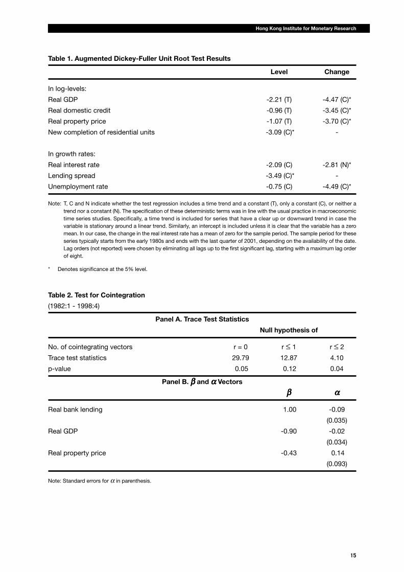
preliminary step, we determine the order of integration of the different time series. Standard augmented

Dickey-Fuller (Dickey and Fuller, 1981) unit root test statistics are reported in Table 1. All data are quarterly

and span the period 1982:1-2001:4. The results suggest that lending, GDP, and property prices are

integrated of order one. The table also includes test results for a few other series that will be used in the

analysis of dynamic relationships, including the real interest rate, the unemployment rate, the lending

spread and the completion of new residential units.

The analysis of the long-run relationship between real lending, real GDP, and real property prices is

based on the multivariable approach to cointegration tests proposed by Johansen (1988, 1991, and

1995).16 The cointegrating VAR model is given by:

xt = B1xt-1 + ..... + Bkxt-k + µ + δτt + εt, (1)

where x is a vector of endogenous variables comprising the log of real bank lending, real GDP and real

property prices. µ is a vector of constants, τ is a deterministic time trend and is a vector of white noise

error terms. The initial estimation period is 1982:1-1998:4, and the data over the last 12 quarters

(1999:1-2001:4) are kept aside to explore the model’s out-of-sample performance. Given that quarterly

data are used, we assume that a VAR(5) model would overfit the data and use this specification as the

start for the sequential testing procedure. In addition to an unrestricted time trend, three centred seasonal

15 The spread turned sharply negative on a few occasions during the Asian financial crisis when speculative pressures on theexchange rate combined with the automatic responses by the currency board led to pronounced increases in short-terminterbank rates. The two interest rates diverged after 2000, reflecting increased competition in the mortgage market.

16 The real interest rate was also included in the initial tests, but did not enter significantly in the cointegrating vector.

6


dummies are allowed. Since F-tests on the groups of regressors indicate that the fourth and fifth lags of

the different variables, the time trend and the seasonal dummies are insignificant, we re-estimate the

model without these and test the implied restrictions. The resulting p-value is 0.55, indicating that the

restrictions are not rejected by the data. We also perform diagnostic tests for fifth order autocorrelation,

normality, fourth-order Autoregressive Conditional Heteroscedasticity and a heteroscedasticity of the

“White” form. Overall, the tests do not reject the null hypothesis.17 We therefore retain this specification

to test for cointegration.

To proceed, the VAR model can be reformulated in a vector error correction form:

∆xt = C1∆xt-1+.....+Ck-1∆xt-k+C0xt-1+µ +εt. (2)

The Johansen methodology is based on maximum likelihood estimation and aims at testing the rank of

the matrix C0, which indicates the number of long-run relationships between the endogenous variables

in the system.18

The results from a standard trace test are reported in Panel A of Table 2. It appears that the null hypothesis

of no CI vector can be rejected (p = 0.05) but that of at most one CI vector cannot be rejected (p = 0.19).

This implies that the matrix C0 can be factorised as C0 = αβ′, where is a (3x1) vector of loading or

adjustment coefficients and β is a (3x1) vector of cointegrating or long-run coefficients. The cointegrating

coefficients β describe the relationship linking the endogenous variables in the long run. The loading

coefficients α describe the dynamic adjustment of the endogenous variables to the long-run equilibrium

given by β′x. Normalising on real bank lending, Panel B of Table 2 provides the estimates of the parameters

in the CI vector. It is notable that the parameter on real GDP is close to -1, implying that real bank loans

and real income grow proportionally over time. The standard errors for the loading coefficients (α)

indicate that the real bank loans adjust to disequilibria (as captured by deviations from the CI relationship).

By contrast, real property prices and real GDP appear to be weakly exogenous. We furthermore test the

restriction that the parameter on real GDP is -1 in the CI vector, and that real property prices and real

GDP are weakly exogenous. The resulting p-value of 0.58 indicates that these restrictions are not rejected

by the data.

To examine the out-sample-period performance of the model, we compute dynamic forecasts for the

remaining 12 quarters. The results indicate that the forecasts remain within the variance errors throughout

the forecasting period for all the three equations. We thus extend the sample period to 2001:4, and

re-estimate the system. As expected, the estimated cointegrating vector and the loading coefficient are

unchanged. Table 3 reports the final estimates of the CI vector and the feedback parameter for real bank

lending. The long-run elasticity of real bank lending with respect to real property prices is about 0.35, so

that a 10% increase in property prices is associated with a 3.5% increase in real bank lending in the

17 However, the errors in the real GDP equation fail the tests for normality, for the absence of ARCH effects and forheteroscedasticity. Inspection of the residuals from this equation suggests that the sources of the failure are a few outliers inthe mid-1980s. Since F-tests for the significance of the third lag of real property prices and real bank lending are highlysignificant, it seems not possible to further shorten the lag length.

18 For a detailed technical exposition, see Johansen (1995).

7


long run. Note that the feedback parameter for real bank lending is substantial (-0.13), and highly significant

(t = 3.9). Overall, these results indicate a single long-run relationship between property prices, bank

loans and GDP during the sample period, to which the system converges. This finding is compatible

with the existing literature on property price movements in OECD economies.19 Furthermore, the results

suggest that deviations from equilibrium tended to be offset over time through movements in bank

lending. Next we turn to the short-run models for quarterly growth rates of lending and property prices.

4. Dynamic relationships

In this section, we turn to the short-term dynamic relationships between real bank credit, real property

prices and real GDP. The above cointegrating results imply that an error correction term — represented

by the once-lagged cointegration vector — should enter the equation for growth in real bank lending.

We also consider other possible variables that do not enter the cointegration relationship, but may

contribute to short-term movements in lending and property prices, such as changes in the real interest

rate. To obtain parsimonious equations for the growth rate of real bank credit and changes in real

property prices respectively, a general-to-specific approach is followed.

In deriving the dynamic equations, one particular concern is the potential simultaneity bias, given that

property prices and bank lending are highly positively correlated. Indeed, initial regressions suggest

that the current value of credit growth enters in the equation for changes in property prices, and the

current change of property prices is significant in explaining credit growth. Thus, either or both equations

are subject to simultaneity bias of unknown importance. To tackle this issue, we follow Davidson and

MacKinnon (1989, 1993) and use a Hausman test to explore the possible patterns of endogeneity in the

two equations.20

4.1 Credit growth

We start with a general model that includes four lags of the dependent variable (∆l), current and four

lags of real GDP growth (∆y), real property price growth (∆p), and change in real interest rate (∆r), and

one lag of the cointegrating vector (CI).21 Following the general-to-specific approach, the parsimonious

model is obtained by removing insignificant variables step by step, starting with the most insignificant

one as indicated by the t-ratios. Along the process, tests for model reduction are monitored to ensure

that the exclusion of a particular series is not rejected by the data. The final equation obtained for ∆l isas follows:

∆lt = + 0.244*∆lt-2 - 0.313 + 0.239*∆yt + 0.176*∆pt - 0.078*CIt-1 + 0.357*(∆rt-1- ∆rt-2) (3)

(SE) (0.083) (0.107) (0.101) (0.034) (0.026) (0.142)

R2 = 0.57; Sample period: 1984:1 - 2001:4

19 For the latter, see Goodhart and Hofmann (2001).

20 See also Eviews 4 User’s Guide, 2001, pp. 382-383.

21 The real interest rate is measured as the difference between the best lending rate and the percentage change in the CPI overthe past four quarters.

8


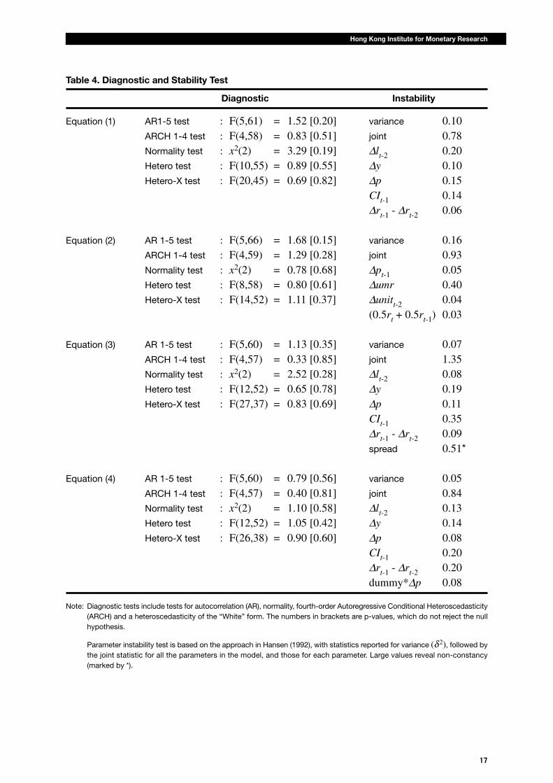
All variables are of correct signs and significant, and various diagnostic tests for the residuals and

parameter instability tests are passed (Table 4). Several observations are worth noting. First, as expected,

the significant error-correction term (CIt-1) suggests that excess bank lending reduces credit growth in

the next period, entailing an adjustment over time to maintain the long-run stable relationship between

real credit, housing price and GDP. Secondly, changes in the real interest rate are significant at lag 1

and 2, but have opposite signs and have roughly equal absolute values. Since the restriction that the

coefficients sum to zero is not rejected, we impose it and re-estimate the model. This specification

implies that changes in real interest rates do not have any long-run impact on credit growth.22

To deal with the potential simultaneity bias due to the presence of ∆p in the equation for ∆l, a Hausman

test is performed. This involves the following procedures. First, an auxiliary regression of ∆p is estimated

on a set of instrumental variables that are likely correlated with ∆p but not with the error term of the ∆lequation.23 Next, we re-estimate the equation for ∆l and add the residuals from the auxiliary regression.

If the OLS estimates of ∆l are consistent, the coefficient on the first stage residuals should not be

significantly different from zero.24 Effectively, the test involves estimating the equation using two-stage

least squares.25 The results indicate that the null hypothesis of consistent OLS estimates cannot be

rejected.26 Thus, movements in property prices seem to have played a structural role in driving credit

growth.

4.2 Property prices

Next we estimate a dynamic model for the growth rate of property prices. To do so, we again start by

fitting a general model with four lags of the dependent and explanatory variables. In addition to ∆l and

∆y, we also include changes in the unemployment rate (∆umr) and the growth rate of the completion of

new residential units (∆unit). A rise in the unemployment rate implies increased uncertainty about

future income growth, and thus could negatively impact on the demand for housing services and

investment in properties. Growth in the completion of new residential units is intended to capture the

supply-side influence on property prices. The general-to-specific approach gives rise to an equation

22 This is perhaps not surprising, considering the difficulties in disentangling the effects of interest rate changes on the demandand supply of bank credit in this framework.

23 The natural choice for instruments is to use the predetermined variables in the two short-run equations, that is, all variablesexcept the current ∆p and ∆l.

24 A pedagogic explanation of the testing strategy is given in Pindyck and Rubinfeld (1991).

25 Another possible way of examining the relationship between property prices and bank lending is the Granger causality test,which assesses whether past values of one variable is useful for predicting future values of another. In the context of thisstudy, the Granger causality test is not appropriate as we are concerned about the contemporaneous correlation between thetwo variables.

26 Specifically, the residuals from the auxiliary regression were not significantly different from zero with a p-value of 0.55.

9


that relates ∆p to its own lag, the current growth in real credit, the change in the unemployment rate

(∆umr), and a twice-lagged growth rate of the completion of new units.27

In order to determine the potential simultaneity bias, we re-estimate the equation for ∆p using instrumental

variables and find that the coefficient on ∆l is highly insignificant and close to zero.28 Thus, it appears

that the high significance of credit growth in the OLS equation for property prices is spurious and is due

to reverse causality.

Since the instrumental variables estimates indicate that current credit growth is not significant in the

equation for property prices, we remove it from the model and estimate, using OLS, the following

parsimonious equation for changes in property prices.

∆pt = + 0.349*∆pt-1 + 0.013 - 0.048*∆umrt - 0.038*∆unitt-2 - 0.200* (0.5rt + 0.5rt-1) (4)

(SE) (0.104) (0.007) (0.014) (0.026) (0.134)

R2 = 0.41; Sample period: 1984:1 2001:4

It is noted that the interest rate variable becomes close to the conventional significance level after

dropping credit growth. As expected, an increase in the unemployment rate tends to reduce the rate of

change of property prices. Also, a rise in new completion of residential units places downward pressure

on housing prices.

The overall fit of the equation is relatively poor, although the diagnostic and instability tests results are

satisfactory.

This is perhaps not surprising given the empirical difficulties in modelling asset prices. There is a large

literature on the valuation of property prices. It is generally found that economic fundamentals only

explain part of the movements in property prices, which are also influenced by speculative activity and

herd behaviour. Some studies employ the present value relationship as predicted by the standard asset

price valuation models (Campbell, Lo and McKinlay (1997)). Based on the hypothesis that prices equal

the expected discounted sum of future rents, property prices are modelled as a function of expected

27 The estimated equation is:∆pt = + 0.283*∆pt-1- 0.008 + 0.900*∆lt - 0.034*∆umrt - 0.041*∆unitt-2(SE) (0.097) (0.007) (0.248) (0.013) (0.024)

R2 = 0.49; Sample period: 1984:1 - 2001:4

28 The estimates are:∆pt = + 0.040*∆lt + 0.392*∆pt-1 + 0.006 - 0.045*∆umrt - 0.047*∆unitt-2(SE) (0.480) (0.117) (0.009) (0.015) (0.026)

The coefficient on ∆l is insignificantly different from zero with a p-value of 0.93.

10


rents and interest rates.29 Other studies take into account other fundamental variables that help determine

the demand and supply of housing services including income growth, changes in the number of

households and housing stock (Abraham and Hendershott 1996). Kalra, Mihaljek and Duenwald (2000)

and Peng (2002) examine empirical models of property prices in Hong Kong that combine fundamental

variables including interest rates with speculative bubbles. They found that only about half of the

movements in real property prices were explained by fundamental variables, and the rest was attributed

to the build-up of a bubble and its subsequent collapse. It is noted that results presented here are

consistent with these studies. In particular, it supports the notion that property prices have been affected

in an important way by excess optimising or pessimism.

4.4 Regulatory change and credit growth

As noted above, in order to limit the exposure of the banking system to a potential fall in property prices,

banks started to apply a maximum loan-to-value ratio voluntarily from the latter part of 1991. This ratio

was later incorporated into HKMA’s guideline on property lending in 1994. One would expect this

regulatory change to affect the results in two ways. First and most obviously, one would expect any

given increase in property prices to have led to less lending growth after 1991. To examine whether the

response of credit growth to movements in property prices has changed over time, we re-estimate the

equation for ∆l recursively. The results indicate that the coefficients on most variables including ∆y are

generally stable except for some volatility in the early period of the sample. However, the coefficient on

∆p seems to have declined considerably after 1991, breaking the previous standard error bands (see

the middle graph in the second column in Chart 5).

Second, the imposition of the regulatory constraint meant that banks could adopt more stringent lending

criteria in order to restrain demand. One way of doing so was to increase lending rates relative to the

cost of funds. As shown in Chart 4, the lending spread did in fact increase around 1991. Of course, the

rise in the spread might also reflect increased risk control by banks in the face of strong demand for

credit. In any case, it is an indicator of a tightening of credit stance. We therefore included it in the

model.30 The OLS estimates below indicate that the parameter on a lagged lending spread has a negative

sign, as expected, and is significant with a p-value of 0.02. Thus an increase in the spread reduces

credit growth in real terms. Recursive estimates suggest that the parameter on ∆p is more stable (Chart

6).31 In particular, while it still declines around 1991, the fall is much smaller (from about 0.4 to 0.3) than

before. Moreover, it remains within the previous error bands.

29 See Meese and Wallace (1994) for a study of housing prices in the US.

30 In computing the spread we use the best lending rate (against the three-month inter-bank rate).

31 However, instability tests suggest some problems with the coefficient on spread itself (see Table 4).

11


∆lt = + 0.211*∆lt-2 - 0.337 + 0.216*∆yt + 0.186*∆pt + 0.340*(∆rt-1 - ∆rt-2) (5)

(SE) (0.081) (0.105) (0.099) (0.034) (0.137)

- 0.086*CIt-1 - 0.381*spreadt-2

(0.026) (0.176)

R2 = 0.60; Sample period: 1984:1 - 2001:4

Finally, we employ a dummy to capture the regime shift around 1991. The dummy variable (dummy)

takes the value of zero up to the middle of 1991, and that of unity thereafter. The equation for ∆l is then

re-estimated and the term dummy*∆p is included. What this term effectively does is to adjust the

coefficient on ∆p in line with a regime shift in banking lending in 1991.32 The estimates of the equation

are as follows:

∆lt = + 0.232*∆lt-2 - 0.272 + 0.296*∆yt + 0.404*∆pt - 0.067*CIt-1 (6)

(SE) (0.078) (0.102) (0.097) (0.081) (0.025)

+ 0.467*(∆rt-1 - ∆rt-2) - 0.268*dummy*∆pt

(0.138) (0.088)

R2 = 0.63; Sample period 1984:1 - 2001:4

It is noted that the dummy series is highly significant, and that the parameters appear more stable than

earlier. Specifically, recursive estimates of the coefficients provide no evidence of instability, as is shown

in Chart 7. Also, various diagnostic and instability tests are passed. Moreover, a comparison of the

coefficients of ∆p and dummy*∆p suggests that a significant drop in the response of credit growth to

property price occurred in 1991. Taking these estimates literally, a 10% increase in real property prices

would lead to a rise in real bank credit by 4% in the earlier sample period, but by only 1.3% after 1991.

5. Conclusion

The main results of this paper are twofold. First, the strong correlation between credit growth and bank

lending in Hong Kong appears to be due to bank lending adjusting to property prices, rather than the

converse. Thus, the cointegration analysis indicates that property prices are weakly exogenous. Moreover,

the error-correction models show that property prices determine bank lending, but that bank lending

does not appear to influence property prices.

32 We also included a series of the dummy multiplied by the error-correction term to check whether there has been a structuralbreak in the cointegration relationship. The results suggest that this term is not significant.

12


Second, the sensitivity of credit to property prices declined in the early 1990s, as banks tightened credit

standards. The latter reflected in part improved risk management by banks in the face of the strong

credit demand and the booming market. The regulatory change in the early 1990s also played an important

role. In particular, the prudential measures including the maximum loan-to-value ratio of 70% may have

led banks to raise intermediation spreads in the 1990s.

Overall, these results suggest that excessive bank lending was not the root cause of the boom and bust

cycles of the property market in Hong Kong. A more plausible hypothesis is that changing beliefs about

future economic prospects led to shifts in the demand for property for investment and other purposes.

In turn, and given a highly inelastic supply schedule, this led to large swings in prices. With a rising

demand for loans and collateral values, bank lending naturally responded.

Finally, the results indicate that prudential regulation and risk controls by banks have limited the exposure

and vulnerability of the banking sector to swings in property prices. As a result, the banking system

remains in fundamentally sound, despite the bust of the property bubble.

13


References

Abraham, J. M. and P. H. Hendershott (1996), “Bubbles in metropolitan housing markets,” Journal of

Housing Research, 7(2): 191-207.

Bernanke, B. and M. Gertler (1989), “Agency Costs, Net Worth and Business Fluctuations,” American

Economic Review, 79(1): 14-31.

Bernanke, B., M. Gertler and S. Gilchrist (1998), “The Financial Accelerator in a Quantitative Business

Cycle Framework,” NBER Working Paper No. 6455, Cambridge MA: National Bureau of Economic

Research.

BIS (2001), 71st Annual Report.

Borio, C. and P. Lowe (2002), “Asset Prices, Financial and Monetary Stability: Exploring the Nexus,” BIS

Working Paper No. 114, July: Bank for International Settlements.

Campbell, J. Y., A. W. Lo and A. C. McKinlay (1997), The Econometrics of Financial Markets, Princeton:

Princeton University Press.

Collyns, C. and A. Senhadji (2002), “Lending Booms, Real Estate Bubbles and the Asian Crisis,” IMF

Working Paper No. 02/20, Washington D.C.: International Monetary Fund.

Davidson, R. and J. G. MacKinnon (1989), “Testing for Consistency Using Artificial Regressions,”

Econometric Theory, 5: 363-84.

Davidson, R. and J. G. MacKinnon (1993), Estimation and Inference in Econometrics, New York: Oxford

University Press.

Dickey, D. and W. Fuller (1981), “Likelihood Ratio Statistics for Autoregressive Time Series with a Unit

Root,” Econometrica, 49(4): 1057-72.

Drees, B. and C. Pazarbasiouglu (1995), “The Nordic Banking Crises: Pitfalls in Financial Liberalization?

” IMF Working Paper No. 95/61, Washington D.C.: International Monetary Fund.

Eviews 4 User’s Guide (2001), Irvine CA, USA: Quantitative Micro Software.

Girouard, N. and S. Blondal (2001), “House Prices and Economic Activity,” OECD Economics Department

Working Paper No. 279, downloadable from http://www.olis.oecd.org/olis/2001doc.nsf/linkto/eco-

wkp(2001)5.

Goodhart, C. (1995), “Price Stability and Financial Fragility,” in K. Sawamoto, Z. Nakajima and H. Taguchi,

eds., Financial Stability in a Changing Environment: St. Martin’s Press.

Goodhart, C. and B. Hofmann (2001), “Deflation, Credit, and Asset Prices,” paper presented at the

conference ‘The Anatomy of Deflation’, 27-28 April 2001, Claremont McKenna College.

Hansen, B. E. (1992), “Testing for Parameter Instability in Linear Models,” Journal of Policy Modeling, 14

(4): 517-33.

Hofmann, B (2003), “Bank Lending and Property Prices: Some International Evidence,” The Hong Kong

Institute for Monetary Research Working Paper, forthcoming.

IMF (2000), World Economic Outlook, May, Washington D.C.: International Monetary Fund.

Johansen, S. (1988), “Statistical Analysis of Cointegration Vectors,” Journal of Economic Dynamics and

Control, 12(2/3): 231-54.

Johansen, S. (1991), “Estimation and Hypothesis Testing of Cointegration Vectors in Gaussian Vector

Autoregressive Models,” Econometrica, 59(6): 1551-80.

Johansen, S. (1995), Likelihood-based Inference in Cointegrated Vector Autoregressive Models: Oxford

University Press.

14


Kalra, S., D. Mihaljek and C. Duenwald (2000), “Property Prices and Speculative Bubbles: Evidence from

Hong Kong SAR,” IMF Working Paper No. 00/02, Washington D.C.: International Monetary Fund.

Kindleberger, C. (1978), “Manias, Panics and Crashes: A History of Financial Crises,” in C. Kindleberger

and J. Laffarge eds., Financial Crises: Theory, History and Policy: Cambridge University Press.

Kiyotaki, N. and J. Moore (1997), “Credit Cycles,” Journal of Political Economy, 105(2): 211-48.

McCauley, R. N., J. S. Ruud and F. Iacono (1999), Dodging Bullets: Changing U.S. Corporate Capital

Structure in the 1980s and 1990s, Cambridge, Massachusetts, London, England: MIT Press.

Meese R. and N. Wallace (1994), “Testing the Present Value Relation for Housing Prices: Should I Leave

My House in San Francisco?” Journal of Urban Economics, 35(3): 245-66.

Minsky, H. (1982), “Can ‘It’ happen again?” Essays on Instability and Finance, M.E. Sharpe.

Peng, WS. (2002), “What Drives Property Price in Hong Kong?” HKMA Quarterly Bulletin, August.

Peng, WS, L. Cheung and C. Leung (2001), “The Property Market and the Macro-economy,” HKMA

Quarterly Bulletin, May.

Pindyck, R. S. and D. L. Rubinfeld (1991), Econometric Models and Economic Forecasts, 3rd ed., New

York: McGraw-Hill.

15


Table 1. Augmented Dickey-Fuller Unit Root Test Results

Level Change

In log-levels:

Real GDP -2.21 (T) -4.47 (C)*

Real domestic credit -0.96 (T) -3.45 (C)*

Real property price -1.07 (T) -3.70 (C)*

New completion of residential units -3.09 (C)* -

In growth rates:

Real interest rate -2.09 (C) -2.81 (N)*

Lending spread -3.49 (C)* -

Unemployment rate -0.75 (C) -4.49 (C)*

Note: T, C and N indicate whether the test regression includes a time trend and a constant (T), only a constant (C), or neither atrend nor a constant (N). The specification of these deterministic terms was in line with the usual practice in macroeconomictime series studies. Specifically, a time trend is included for series that have a clear up or downward trend in case thevariable is stationary around a linear trend. Similarly, an intercept is included unless it is clear that the variable has a zeromean. In our case, the change in the real interest rate has a mean of zero for the sample period. The sample period for theseseries typically starts from the early 1980s and ends with the last quarter of 2001, depending on the availability of the date.Lag orders (not reported) were chosen by eliminating all lags up to the first significant lag, starting with a maximum lag orderof eight.

* Denotes significance at the 5% level.

Table 2. Test for Cointegration

(1982:1 - 1998:4)

Panel A. Trace Test Statistics

Null hypothesis of

No. of cointegrating vectors r = 0 r ≤ 1 r ≤ 2

Trace test statistics 29.79 12.87 4.10

p-value 0.05 0.12 0.04

Panel B. βββββ and ααααα Vectors

βββββ ααααα

Real bank lending 1.00 -0.09

(0.035)

Real GDP -0.90 -0.02

(0.034)

Real property price -0.43 0.14

(0.093)

Note: Standard errors for α in parenthesis.

16


Table 3. Long-Run Relationship

( 1982:1 - 2001:4 )

CI vector Loading coefficient

βββββ ααααα

Real bank lending 1.00 -0.13

(0.03)

Real GDP -1.00 0.00

Real property price -0.36 0.00

Note: Standard error for α in parenthesis.

17


Table 4. Diagnostic and Stability Test

Diagnostic Instability

Equation (1) AR1-5 test : F(5,61) = 1.52 [0.20] variance 0.10ARCH 1-4 test : F(4,58) = 0.83 [0.51] joint 0.78Normality test : x2(2) = 3.29 [0.19] ∆lt-2 0.20Hetero test : F(10,55) = 0.89 [0.55] ∆y 0.10Hetero-X test : F(20,45) = 0.69 [0.82] ∆p 0.15

CIt-1 0.14∆rt-1 - ∆rt-2 0.06

Equation (2) AR 1-5 test : F(5,66) = 1.68 [0.15] variance 0.16ARCH 1-4 test : F(4,59) = 1.29 [0.28] joint 0.93Normality test : x2(2) = 0.78 [0.68] ∆pt-1 0.05Hetero test : F(8,58) = 0.80 [0.61] ∆umr 0.40Hetero-X test : F(14,52) = 1.11 [0.37] ∆unitt-2 0.04

(0.5rt + 0.5rt-1) 0.03

Equation (3) AR 1-5 test : F(5,60) = 1.13 [0.35] variance 0.07ARCH 1-4 test : F(4,57) = 0.33 [0.85] joint 1.35Normality test : x2(2) = 2.52 [0.28] ∆lt-2 0.08Hetero test : F(12,52) = 0.65 [0.78] ∆y 0.19Hetero-X test : F(27,37) = 0.83 [0.69] ∆p 0.11

CIt-1 0.35∆rt-1 - ∆rt-2 0.09spread 0.51*

Equation (4) AR 1-5 test : F(5,60) = 0.79 [0.56] variance 0.05ARCH 1-4 test : F(4,57) = 0.40 [0.81] joint 0.84Normality test : x2(2) = 1.10 [0.58] ∆lt-2 0.13Hetero test : F(12,52) = 1.05 [0.42] ∆y 0.14Hetero-X test : F(26,38) = 0.90 [0.60] ∆p 0.08

CIt-1 0.20∆rt-1 - ∆rt-2 0.20dummy*∆p 0.08

Note: Diagnostic tests include tests for autocorrelation (AR), normality, fourth-order Autoregressive Conditional Heteroscedasticity(ARCH) and a heteroscedasticity of the “White” form. The numbers in brackets are p-values, which do not reject the nullhypothesis.

Parameter instability test is based on the approach in Hansen (1992), with statistics reported for variance (δ 2), followed by

the joint statistic for all the parameters in the model, and those for each parameter. Large values reveal non-constancy(marked by *).

18


Chart 1. Residential Property Prices

2.0

2.5

3.0

3.5

4.0

4.5

5.0

2.0

2.5

3.0

3.5

4.0

4.5

5.0

82 84 86 88 90 92 94 96 98 00

Nominal property price (Q3 97=100)Real roperty price (Q3 97=100)

loglog

Chart 2. Property Prices, Domestic Credit and GDP

(Normalised)

-3

-2

-1

0

1

2

-3

-2

-1

0

1

2

82 84 86 88 90 92 94 96 98 00

Real domestic loanReal GDPReal property price

log log

19


Chart 3. Annual Growth of Property Prices and Domestic Credit

-60

-40

-20

0

20

40

60

-60

-40

-20

0

20

40

60

82 84 86 88 90 92 94 96 98 00

Real domestic loanReal property price

% %

Chart 4. Bank Lending Spreads

-1

0

1

2

3

4

5

6

-1

0

1

2

3

4

5

6

82 84 86 88 90 92 94 96 98 00

Best lending rate over 3M HIBORMortgage rate over 3M HIBOR

% %

20


Chart 5. Recursive Estimates of Parameters in Equation dl without Spread

1990 1995 2000

0.00

0.25

0.50dl_2 x +/-2SE

1990 1995 2000

-2

-1

0

Constant x +/-2SE

1990 1995 20000.00

0.25

0.50 dy x +/-2SE

1990 1995 2000

0.25

0.50

0.75dp x +/-2SE

1990 1995 2000-0.50

-0.25

0.00

CI_1 x +/-2SE

1990 1995 2000

0.0

0.5

1.0(dr_1-dr_2) x +/-2SE

Chart 6. Recursive Estimates of Equation for dl with Spread

1990 1995 2000

0.00

0.25

0.50 dl_2 x +/-2SE

1990 1995 2000

-2

-1

0

Constant x +/-2SE

1990 1995 2000

0.00

0.25

0.50 dy x +/-2SE

1990 1995 2000

0.25

0.50

0.75 dp x +/-2SE

1990 1995 2000

-0.4

-0.2

0.0

CI_1 x +/-2SE

1990 1995 2000

0.0

0.5

1.0 (dr_1-dr_2) x +/-2SE

1990 1995 2000

-1

0

spread_2 x +/-2SE

21


Chart 7. Recursive Estimates of Parameters in Equation for dl Equation with a Dummy

1990 1995 2000

0.00

0.25

0.50 dl_2 x +/-2SE

1990 1995 2000

-2

-1

0

Constant x +/-2SE

1990 1995 2000

0.25

0.50dy x +/-2SE

1990 1995 2000

0.25

0.50

0.75

dp x +/-2SE

1990 1995 2000

-0.50

-0.25

0.00

CI_1 x +/-2SE

1990 1995 2000

0.0

0.5

1.0 (dr_1-dr_2) x +/-2SE

1990 1995 2000

-0.5

0.0

dumdp x +/-2SE

hong kong institute for onetary esearch · study of the nexus between bank lending, property prices...

Documents