arX

iv:m

ath.

CO

/020

2034

v2

4 D

ec 2

002

Homogeneous Multivariate Polynomialswith the Half-Plane Property

Young-Bin ChoeDepartment of Combinatorics and Optimization

University of WaterlooWaterloo, Ontario N2L 3G1, CANADA

ybchoe@math.uwaterloo.ca

James G. OxleyDepartment of MathematicsLouisiana State University

Baton Rouge, LA 70803-4918, USAoxley@math.lsu.edu

Alan D. SokalDepartment of PhysicsNew York University

New York, NY 10003, USAsokal@nyu.edu

David G. WagnerDepartment of Combinatorics and Optimization

University of WaterlooWaterloo, Ontario N2L 3G1, CANADA

dgwagner@math.uwaterloo.ca

February 4, 2002revised November 23, 2002

Abstract

A polynomial P in n complex variables is said to have the “half-plane prop-erty” (or Hurwitz property) if it is nonvanishing whenever all the variables liein the open right half-plane. Such polynomials arise in combinatorics, relia-bility theory, electrical circuit theory and statistical mechanics. A particularlyimportant case is when the polynomial is homogeneous and multiaffine: then itis the (weighted) generating polynomial of an r-uniform set system. We provethat the support (set of nonzero coefficients) of a homogeneous multiaffine poly-nomial with the half-plane property is necessarily the set of bases of a matroid.Conversely, we ask: For which matroids M does the basis generating polynomialPB(M) have the half-plane property? Not all matroids have the half-plane prop-erty, but we find large classes that do: all sixth-root-of-unity matroids, and asubclass of transversal (or cotransversal) matroids that we call “nice”. Further-more, the class of matroids with the half-plane property is closed under minors,duality, direct sums, 2-sums, series and parallel connection, full-rank matroidunion, and some special cases of principal truncation, principal extension, prin-cipal cotruncation and principal coextension. Our positive results depend ontwo distinct (and apparently unrelated) methods for constructing polynomialswith the half-plane property: a determinant construction (exploiting “energy”arguments), and a permanent construction (exploiting the Heilmann–Lieb the-orem on matching polynomials). We conclude with a list of open questions.

KEY WORDS: Graph, matroid, jump system, abstract simplicial complex, span-ning tree, basis, generating polynomial, reliability polynomial, Brown–Colbourn con-jecture, half-plane property, Hurwitz polynomial, positive rational function, Lee–Yang theorem, Heilmann–Lieb theorem, matching polynomial, Grace–Walsh–Szegocoincidence theorem, matrix-tree theorem, electrical network, nonnegative matrix,determinant, permanent.

2000 MATHEMATICS SUBJECT CLASSIFICATION: Primary 05B35; Sec-ondary 05C99, 05E99, 15A15, 15A48, 30C15, 32A99, 82B20, 94C05.

RUNNING HEAD: Polynomials with the Half-Plane Property

Contents

1 Introduction 4

2 Polynomials and the half-plane property 102.1 Basic definitions . . . . . . . . . . . . . . . . . . . . . . . . . . . . . . 102.2 Shifted half-plane property and leading part . . . . . . . . . . . . . . 112.3 Real-part-positive rational functions . . . . . . . . . . . . . . . . . . . 122.4 Derivatives . . . . . . . . . . . . . . . . . . . . . . . . . . . . . . . . . 142.5 The Grace–Walsh–Szego coincidence theorem . . . . . . . . . . . . . 162.6 Algorithms . . . . . . . . . . . . . . . . . . . . . . . . . . . . . . . . . 17

3 The local half-plane property 18

4 Constructions 214.1 Deletion and contraction . . . . . . . . . . . . . . . . . . . . . . . . . 214.2 Duality . . . . . . . . . . . . . . . . . . . . . . . . . . . . . . . . . . . 224.3 Direct sum . . . . . . . . . . . . . . . . . . . . . . . . . . . . . . . . . 234.4 Parallel connection, series connection, and 2-sum . . . . . . . . . . . 244.5 Principal truncation and principal extension . . . . . . . . . . . . . . 274.6 Principal cotruncation and principal coextension . . . . . . . . . . . . 294.7 Multiaffine part and full-rank matroid union . . . . . . . . . . . . . . 314.8 “Folding mod 2” and convolution . . . . . . . . . . . . . . . . . . . . 33

5 Necessary and sufficient condition 365.1 General case . . . . . . . . . . . . . . . . . . . . . . . . . . . . . . . . 365.2 Rank-2 case . . . . . . . . . . . . . . . . . . . . . . . . . . . . . . . . 37

6 Necessary conditions I: Same-phase property 41

2

7 Necessary conditions II: Matroidal support 457.1 The exchangeability theorem . . . . . . . . . . . . . . . . . . . . . . . 457.2 The weak half-plane property . . . . . . . . . . . . . . . . . . . . . . 49

8 The determinant condition and 6√

1-matroids 508.1 The determinant condition . . . . . . . . . . . . . . . . . . . . . . . . 508.2 (F,G)-representability and 6

√1-matroids . . . . . . . . . . . . . . . . 51

9 Uniform matroids 589.1 Half-plane property . . . . . . . . . . . . . . . . . . . . . . . . . . . . 589.2 Brown–Colbourn property . . . . . . . . . . . . . . . . . . . . . . . . 60

10 The permanent condition: Transversal and cotransversal matroids 6110.1 Heilmann–Lieb theorem . . . . . . . . . . . . . . . . . . . . . . . . . 6110.2 Application to transversal matroids . . . . . . . . . . . . . . . . . . . 6310.3 Examples . . . . . . . . . . . . . . . . . . . . . . . . . . . . . . . . . 6510.4 Rank-3 transversal matroids . . . . . . . . . . . . . . . . . . . . . . . 7410.5 A wild speculation . . . . . . . . . . . . . . . . . . . . . . . . . . . . 75

11 Counterexamples 76

12 Numerical experiments 80

13 Open questions 8213.1 The strong half-plane property . . . . . . . . . . . . . . . . . . . . . . 8213.2 Same-phase theorem . . . . . . . . . . . . . . . . . . . . . . . . . . . 8313.3 Support of polynomials with the half-plane property . . . . . . . . . . 8313.4 (F,G)-representability of matroids . . . . . . . . . . . . . . . . . . . . 8413.5 Determinant class, permanent class, and the half-plane property . . . 8513.6 Half-plane property for transversal matroids . . . . . . . . . . . . . . 8713.7 Half-plane property for 7-element rank-3 matroids . . . . . . . . . . . 8813.8 Algorithms . . . . . . . . . . . . . . . . . . . . . . . . . . . . . . . . . 88

A Matroids considered in this paper 89A.1 Rank-3 matroids on 6 elements . . . . . . . . . . . . . . . . . . . . . 89A.2 Rank-3 matroids on 7 elements . . . . . . . . . . . . . . . . . . . . . 90

A.2.1 Matroids with a 4-point line . . . . . . . . . . . . . . . . . . . 91A.2.2 The Fano matroid F7 and its relaxations . . . . . . . . . . . . 93A.2.3 P7 and its relaxations . . . . . . . . . . . . . . . . . . . . . . . 94

A.3 Some rank-3 matroids on 8 or 9 elements . . . . . . . . . . . . . . . . 94A.4 Some rank-4 matroids on 8 elements . . . . . . . . . . . . . . . . . . 97A.5 Some transversal matroids . . . . . . . . . . . . . . . . . . . . . . . . 98

B (F, {1})-representability of matroids 98

3

1 Introduction

It seems that the theory of polynomials, linear in eachvariable, that do not have zeros in a given multidisk ora more general set, has a long way to go, and has sofar unnoticed connections to various other concepts inmathematics.

— Aimo Hinkkanen [37, p. 288]

Let us consider a connected graphG = (V,E) as an electrical network, by assigningto each edge e ∈ E a complex number xe, called its conductance (or admittance).1

The node voltages {ϕi}i∈V and current inflows {Ji}i∈V then satisfy the linear systemL(x)ϕ = J , where L(x) is the edge-weighted Laplacian matrix for G [that is, L(x) =BXBT where B is the directed vertex-edge incidence matrix for any orientation ofG, and X = diag({xe})]. On physical grounds we expect that if Rexe > 0 for all e(i.e. every branch is dissipative), then the network is uniquely solvable once we fixthe voltage at a single reference node i0 ∈ V , or in other words that the i0th principalcofactor of L(x) is nonzero. Now, by the matrix-tree theorem [9, 17, 16, 80], eachprincipal cofactor of L(x) equals the spanning-tree sum

TG(x) =∑

trees T⊆E

xT , (1.1)

where we have used the shorthand x = {xe}e∈E and xT =∏

e∈T xe. We thereforeconjecture:

Theorem 1.1 Let G be a connected graph. Then the spanning-tree polynomial TG

has the “half-plane property”, i.e. Rexe > 0 for all e implies TG(x) 6= 0.

The proof of Theorem 1.1 is not difficult: Consider any nonzero complex vectorϕ = {ϕi}i∈V satisfying ϕi0 = 0. Because G is connected, we have BTϕ 6= 0. Therefore,the quantity

ϕ∗L(x)ϕ = ϕ∗BXBTϕ =∑

e∈E

|(BTϕ)e|2 xe (1.2)

has strictly positive real part whenever Rexe > 0 for all e; so in particular (BXBTϕ)i 6=0 for some i 6= i0. It follows that the submatrix of L(x) obtained by suppressing thei0th row and column is nonsingular, and so has a nonzero determinant. Theorem 1.1then follows from the matrix-tree theorem.2

1 In this paper all graphs are finite and undirected. Loops and multiple edges are allowed unlessspecified otherwise.

2 This proof is well known in the circuit-theory literature: see e.g. [18, Section 2.7] as well asthe related results in [23, pp. 398–401, 430–431 and 850–851] [58, pp. 52–53 and 67–69]. It has,moreover, a natural physical interpretation: if ϕ = {ϕi}i∈V are the node voltages, then the real partof the quadratic form (1.2) is the total power dissipated in the circuit. We thank Charles Desoerand Paul Penfield for pointing out references [23, 58].

4

An immediate corollary of Theorem 1.1 is that the complementary spanning-treepolynomial

TG(x) =∑

trees T⊆E

xE\T (1.3)

also has the half-plane property, since

TG(x) = xE TG(1/x) (1.4)

and the map xe 7→ 1/xe takes the right half-plane onto itself.From a combinatorial point of view, the noteworthy fact is that the spanning

trees of G constitute the bases of the graphic matroid M(G), and their comple-

ments constitute the bases of the cographic matroid M∗(G). So TG and TG are the(multivariate) basis generating polynomials for M(G) and M∗(G), respectively. Thisnaturally suggests generalizing Theorem 1.1 to more general matroids and, perhaps,to more general set systems. Before posing these questions precisely, we need to fixsome notation and terminology.

A set system (or hypergraph) S on the (finite) ground set E is simply a collection Sof subsets of E. Given any set system S on E, we define its (multivariate) generatingpolynomial to be

PS(x) =∑

S∈S

xS , (1.5)

where x = {xe}e∈E are commuting indeterminates (which we shall usually take tobe complex variables). The rank of a set system is the maximum cardinality of itsmembers (by convention we set rank = −∞ if S = ∅); equivalently, it is the degreeof the generating polynomial PS . A set system S is r-uniform if |S| = r for all S ∈ S,or equivalently if its generating polynomial PS is homogeneous of degree r.

An abstract simplicial complex (or complex for short) is a set system S satisfying

(I1) ∅ ∈ S.

(I2) If S ∈ S and S ′ ⊆ S, then S ′ ∈ S (“S is hereditary downwards”).

The members S of a complex are called faces , and the maximal members (with respectto set-theoretic inclusion) are called facets . A complex is called pure (of rank r) if allits facets have the same cardinality r.

A complex S is called a matroid complex if it satisfies the further condition

(I3) If S1, S2 ∈ S and |S1| < |S2|, then there exists an element e ∈S2 \ S1 such that S1 ∪ {e} ∈ S (“independence augmentation axiomfor matroids”).

The faces of a matroid complex are called the independent sets of the matroid; thefacets (i.e. the maximal independent sets) are called bases . It is easy to prove thatevery matroid complex is pure, i.e. all bases have the same cardinality r, called therank of the matroid. Moreover, it is not difficult to show that a collection B of subsetsof E is the collection of bases of a matroid on E if and only if it satisfies the followingtwo conditions:

5

(B1) B is nonempty.

(B2) If B1, B2 ∈ B and x ∈ B1 \ B2, then there exists y ∈ B2 \ B1 suchthat (B1 \ x) ∪ {y} ∈ B (“basis exchange axiom for matroids”).

For more information on matroid theory, see [55].We shall be particularly interested in the basis generating polynomial of a matroid

M ,

PB(M)(x) =∑

B∈B(M)

xB . (1.6)

We can now pose the following questions concerning possible extensions of Theo-rem 1.1:

Question 1.2 For which matroids M does the basis generating polynomial PB(M)

have the half-plane property?

More generally:

Question 1.3 For which r-uniform set systems S does the generating polynomial PS

have the half-plane property?

Our original conjecture was that all matroids (and no non-matroidal set systems)have the half-plane property. That would be nice and neat, but it turns out to befalse; and the truth is considerably more interesting and subtle. Our conjecture is halfright: an r-uniform set system with the half-plane property is necessarily the set ofbases of a matroid (Theorem 7.1). But not every matroid has the half-plane property,and we do not yet have a complete characterization of those that do. Nevertheless,we can find large classes of matroids with the half-plane property:

(a) Every sixth-root-of-unity matroid [78] has the half-plane property (Theorem 8.1and Corollary 8.2). This class properly includes the regular matroids, which inturn properly include the graphic and cographic matroids. The proof of Theo-rem 8.1 is, in fact, a direct generalization of the proof just given for Theorem 1.1.

(b) Every uniform matroid has the half-plane property, and indeed has the (stronger)“Brown–Colbourn property” (Section 9).

(c) A significant subclass of transversal matroids — those we call “nice” — have thehalf-plane property (Section 10). Indeed, it may well be true that all transversalmatroids have the half-plane property, but we have no idea how to prove this.

(d) All matroids of rank or corank at most 2 have the half-plane property (Corol-lary 5.5), as do all matroids on a ground set of at most 6 elements (Proposi-tion 10.4).

6

(e) The class of matroids with the half-plane property is closed under minors, dual-ity, direct sums, 2-sums, series and parallel connection, full-rank matroid union,and some special cases of principal truncation, principal extension, principalcotruncation and principal coextension (Section 4).

Moreover, we can show that certain matroids do not have the half-plane property:among these are the Fano matroid F7, the non-Fano matroid F−

7 , their relaxationsF−−

7 , F−37 and M(K4) + e, the matroids P8, P

′8 and P ′′

8 , the Pappus and non-Pappusmatroids, the free extension (non-Pappus \ 9) + e, and all their duals (Section 11).The first six of these examples are minor-minimal, and we conjecture that the othersare as well; but we strongly suspect that this list is incomplete, and indeed we considerit likely that the set of minor-minimal non-half-plane-property matroids is infinite.

More generally, we shall consider homogeneous multiaffine polynomials P (x) =∑S⊆E,|S|=r aSx

S with arbitrary complex coefficients aS (not necessarily 0 or 1). Weshall prove two necessary conditions for P 6≡ 0 to have the half-plane property:

(a) P must have the “same-phase property”, i.e. all the nonzero coefficients aS

must have the same phase (Theorem 6.1). So without loss of generality we canassume that all the aS are nonnegative.

(b) The support supp(P ) = {S ⊆ E: aS 6= 0} must be the collection of bases of amatroid (Theorem 7.1).

This latter fact is particularly striking: it shows that matroids arise naturally from aconsideration of homogeneous multiaffine polynomials with the half-plane property.We do not know whether the converse of Theorem 7.1 is true, i.e. whether for everymatroid M there exists a homogeneous multiaffine polynomial P with the half-planeproperty such that supp(P ) = B(M). But it is true, at least, for all matroids repre-sentable over C (Corollary 8.2).

We shall also also give two sufficient conditions for a homogeneous multiaffinepolynomial P to have the half-plane property (or be identically zero):

(a) Determinant condition (Theorem 8.1): aS = |det (A ↾ S)|2 for some r × ncomplex matrix A [here n = |E|, and A ↾ S denotes the square submatrixof A using the columns indexed by the set S]. This corresponds to P (x) =det (AXA∗) where X = diag({xe}) and ∗ denotes Hermitian conjugate.

(b) Permanent condition (Theorem 10.2): aS = per(Λ ↾ S) for some r× n nonneg-ative matrix Λ. This corresponds to P (x) = per(ΛX).

Unfortunately, the relationship between these sufficient conditions and the half-planeproperty looks complicated. Neither family of polynomials contains the other; theirintersection is nonempty; and their union is a proper subset of the set of all homoge-neous multiaffine polynomials with the half-plane property.

These questions also have a close connection with reliability theory [19]. Considera finite set E of communication channels, which fail independently with probabilities

7

{qe}e∈E. Let S be a set system on E, whose members we shall interpret as thesets of failed channels that allow the system as a whole to be operational. Thenthe probability that the system is operational is given by the multivariate reliabilitypolynomial

RelS(q) =∑

A∈S

qA (1 − q)E\A (1.7)

where q = {qe}e∈E. This is easily related to the multivariate generating polynomial

PS(x) =∑

A∈S

xA (1.8)

by

RelS(q) = (1 − q)E PS

( q

1 − q

)(1.9)

PS(x) = (1 + x)E RelS

( x

1 + x

)(1.10)

In the reliability context it is natural to assume that S is a complex, i.e. that Scontains ∅ and is closed under taking subsets. Indeed, the simplest case arises whenG = (V,E) is a connected graph and we declare the system to be operational ifthe non-failed edges form a connected spanning subgraph (this is the “all-terminalreliability”). In this case S is the set of complements of connected spanning subgraphsof G, i.e. the family I(M∗(G)) of independent sets of the cographic matroid M∗(G).Our Holy Grail is the following:

Conjecture 1.4 (multivariate Brown–Colbourn conjecture [10, 70]) Let G bea connected graph. If |qe| > 1 for all e, then RelI(M∗(G))(q) 6= 0. Equivalently, if G isloopless and Re xe < −1/2 for all e, then PI(M∗(G))(x) 6= 0.

(Note that a loop in G corresponds to a coloop in M∗(G). Each loop in G has noeffect on the reliability polynomial but multiplies the independent-set polynomial ofM∗(G) by a factor 1 + xe, leading to a root at xe = −1. This is why, in discussingthe roots of PI(M∗(G)), we need to assume that G is loopless.)

We are at present quite far from a proof of Conjecture 1.4. One of us has provenConjecture 1.4 for the special case of series-parallel graphs [70, Remark 3 in Section4.1]; earlier, another one of us had proven the corresponding univariate result, i.e.when all the qe take the same value [73]. But series-parallel graphs are a small subsetof planar graphs, and an even smaller subset of all graphs!

Nonetheless one can dream, and even lacking a proof of Conjecture 1.4 it is rea-sonable to ask whether stronger results might be true. For example:

Question 1.5 Which (coloopless) matroids M have the “Brown–Colbourn property”,i.e. Re xe < −1/2 for all e implies PI(M)(x) 6= 0?

8

Aside from the cographic (or equivalently, graphic) matroids of series-parallel graphs,we can prove the Brown–Colbourn property for uniform matroids Ur,n with 0 ≤ r <n (the condition r < n corresponds precisely to forbidding coloops): this followsimmediately from the corresponding univariate result [73, Proposition 7.3] combinedwith the Grace–Walsh–Szego coincidence theorem (see Section 9). On the otherhand, it is easy to show (Corollary 2.3) that the Brown–Colbourn property for PI(M)

implies the half-plane property for PB(M). So the results of this paper imply that theBrown–Colbourn property fails for many matroids (e.g. F7, F

−7 , . . . ) and for all pure

complexes that are not matroidal.One purpose of this paper is, therefore, to serve as a “warm-up” for an attack on

the Brown–Colbourn property, by studying first a property (the half-plane property)that is a necessary condition for the Brown–Colbourn property and may be easier tocharacterize. But the results of our investigation show that the half-plane propertyis very interesting in its own right!

Our study of polynomials with the half-plane property can also be viewed inthe wider context of theorems asserting that some combinatorially interesting classof multivariate polynomials are nonvanishing in some large domain of complex n-space. Theorems of this kind include the Lee–Yang theorem on ferromagnetic Isingmodels and generalizations thereof [46, 68, 47, 37] and the Heilmann–Lieb theoremon matching polynomials [35] (discussed in Section 10.1 below). Useful tools formanipulating such polynomials include the Grace–Walsh–Szego coincidence theorem[31, 71, 74, 51] (see Section 2.5), the Asano contraction lemma [3, 63, 37] and theHinkkanen composition theorem [37] (see Section 4.8).

The plan of this paper is as follows: In Section 2 we discuss the basic propertiesof multivariate polynomials with the half-plane property, including their importantconnection with real-part-positive rational functions. In Section 3 we discuss a keycriterion that we call the “local half-plane property”. In Section 4 we describe a largenumber of constructions that preserve the half-plane property; most of these are mo-tivated by standard operations on matroids. In Section 5 we provide a necessary andsufficient condition for a polynomial to have the half-plane property; this conditionwill play an important role in finding counterexamples. We also provide a simpleexplicit criterion in the rank-2 case. In Section 6 we prove that, in a homogeneouspolynomial with the half-plane property, all the nonzero coefficients must have thesame phase. In Section 7 we prove that the support of a homogeneous multiaffinepolynomial must be the collection of bases of a matroid; we also prove a generaliza-tion to the non-multiaffine case. In Section 8 we give the “determinant construction”,and deduce as a corollary that every sixth-root-of-unity matroid has the half-planeproperty. This section also contains some results on (F,G)-representability of ma-troids that may be of independent interest. In Section 9 we prove that every uniformmatroid has the half-plane property, and indeed has the Brown–Colbourn property.In Section 10 we give the “permanent construction”, and deduce as a corollary thata certain subclass of transversal matroids (those we call “nice”) have the half-planeproperty; we also give numerous examples of nice and non-nice transversal matroids.

9

In Section 11 we give several examples of matroids that do not have the half-planeproperty. In Section 12 we report our numerical experiments on matroids for whichwe have been unable to prove or disprove the half-plane property. We conclude, inSection 13, with a list of open questions. In Appendix A we provide, for the conve-nience of the reader, a list of the matroids considered in this paper, along with briefsummaries of their properties. In Appendix B we analyze the (F, {1})-representabilityof matroids.

Note Added (November 2002): Gordon Royle and one of the authors (A.D.S.)have recently discovered — to our great surprise — that the Brown–Colbourn con-jecture is false! The multivariate Brown–Colbourn conjecture is false already for thesimplest non-series-parallel graph, namely the complete graph K4. The univariateBrown–Colbourn conjecture is false for certain simple planar graphs that can be ob-tained from K4 by parallel and series extension of edges. This work will be reportedseparately [61].

2 Polynomials and the half-plane property

Our main interest is in polynomials that are homogeneous of degree r and aremultiaffine (i.e. of degree ≤ 1 in each variable separately): these include the generat-ing polynomials of r-uniform set systems and, more specifically, the basis generatingpolynomials of rank-r matroids. However, many of our results will be valid for homo-geneous polynomials that are not necessarily multiaffine, or for multiaffine polyno-mials that are not necessarily homogeneous, or (sometimes) for general polynomials.We shall endeavor to state our results in whatever degree of generality seems mostnatural, without being pedantic.

2.1 Basic definitions

Let P (x) =∑

mamx

m be a polynomial with complex coefficients in the variablesx = {xe}e∈E . We call the finite set E = E(P ) the ground set of P , and we callits members elements. We shall generally use the letter n to denote the cardinalityof E; often we shall simply take E to be [n] = {1, . . . , n}. In P , the sum rangesover all multi-indices m (that is, functions m: E → N), and only finitely many of

the coefficients am are nonzero. The degree of the monomial xm =∏

e∈E xm(e)e is

|m| =∑

e∈E m(e), and the degree of P is degP = max{|m|: am 6= 0}. We say that Pis homogeneous of degree r if am = 0 whenever |m| 6= r. For e ∈ E, the degree of P inxe is dege P = max{m(e): am 6= 0}. We say that P is affine in e if dege P ≤ 1, andwe say that P is multiaffine if it is affine in e for all e ∈ E. A multiaffine polynomialcan be written in the form P (x) =

∑S⊆E aSx

S.The support of a polynomial P (x) =

∑mamx

m is the set of multi-indices withnonzero coefficients:

supp(P ) = {m: am 6= 0} . (2.1)

10

In the case of a multiaffine polynomial P (x) =∑

S⊆E aSxS, we identify multi-indices

with subsets of E, so that

supp(P ) = {S ⊆ E: aS 6= 0} . (2.2)

If D is a domain (connected open set) in Cn, we denote by FD the set of allfunctions analytic in D that are either nonvanishing in D or else identically zero. ByHurwitz’s theorem3, FD is closed in the topology of uniform convergence on compactsubsets of D. (That is why we included the phrase “or else identically zero” in thedefinition of FD: it takes care of a trivial degenerate case in a convenient way.)

Let us now suppose that D = D1 × · · · ×Dn where the Di are domains in C. Iff ∈ FD and we fix some of the variables (say x1, . . . , xm) to particular values x

(0)1 ∈ D1,

. . . , x(0)m ∈ Dm, then clearly f(x

(0)1 , . . . , x

(0)m , · ) ∈ FDm+1×···×Dn . But more is true, at

least if f ∈ FD is also continuous in the closure D = D1 × · · · ×Dn: then we can fixx

(0)1 ∈ D1, . . . , x

(0)m ∈ Dm and we still have f(x

(0)1 , . . . , x

(0)m , · ) ∈ FDm+1×···×Dn (again

by Hurwitz’s theorem). That is, we can fix some variables even on the boundary of thedomain, and as a function of the remaining variables, f must be either nonvanishingor else identically zero.

We denote by H the open right half-plane {x ∈ C: Re x > 0}, and by H theclosed right half-plane {x ∈ C: Rex ≥ 0}. If the polynomial P in n variables belongsto FHn (i.e. is either nonvanishing in the product of open right half-planes or elseidentically zero), we say that P has the half-plane property .4 The discussion of theprevious paragraph has the following corollary:

Proposition 2.1 Let P have the half-plane property, let E ′ be a subset of the ground

set E = E(P ), and fix x′ ∈ HE′

. Then P (x′, · ), considered as a polynomial on theground set E \E ′, has the half-plane property. In particular, this holds when we takex′ = 0.

2.2 Shifted half-plane property and leading part

Let us denote by Hθ,K the rotated translated open half-plane {x ∈ C: Re (e−iθx) >K}. If the polynomial P in n variables belongs to FHn

θ,Kfor some θ and K, we say

3 Hurwitz’s theorem states that if D is a domain in Cn and (fk) are nonvanishing analyticfunctions on D that converge to f uniformly on compact subsets of D, then f is either nonvanishingor else identically zero. Hurwitz’s theorem for n = 1 is proved in most standard texts on the theoryof analytic functions of a single complex variable (see e.g. [1, p. 176]). Surprisingly, we have beenunable to find Hurwitz’s theorem proven for general n in any standard text on several complexvariables (but see [42, p. 306] and [68, p. 337]). So here, for completeness, is the sketch of a proof:Suppose that f(c) = 0 for some c = (c1, . . . , cn) ∈ D, and let D′ ⊂ D be a small polydisc centeredat c. Applying the single-variable Hurwitz theorem, we conclude that f(z1, c2, . . . , cn) = 0 for all z1

such that (z1, c2, . . . , cn) ∈ D′. Applying the same argument repeatedly in the variables z2, . . . , zn,we conclude that f is identically vanishing on D′ and hence, by analytic continuation, also on D.

4 In the engineering literature, polynomials P 6≡ 0 with the half-plane property are termedwidest-sense Hurwitz polynomials : see e.g. [26].

11

that P has the shifted half-plane property . In particular, if P ∈ FHnπ,1/2

, we say that

P has the Brown–Colbourn property .If P is a polynomial of degree r, we denote by P ♯ the polynomial consisting of

those terms in P that have degree r, and we call it the leading part of P . Clearly P ♯

is homogeneous of degree r. Moreover, it is easy to see that

P ♯(x) = limζ→∞

ζ−rP (ζx) (2.3)

as ζ tends to infinity in C, uniformly for x in compact subsets of Cn. Using Hurwitz’stheorem, we deduce immediately that:

Proposition 2.2 If P has the shifted half-plane property, then P ♯ has the half-planeproperty [and more generally belongs to FHn

θ′,0for all θ′].

Corollary 2.3 Let M be a matroid. If the independent-set generating polynomialPI(M) has the Brown–Colbourn property, then the basis generating polynomial PB(M)

has the half-plane property.

Henceforth we shall say that a set system S (resp. a matroid M) “has the half-plane property” if its generating polynomial PS (resp. its basis generating polynomialPB(M)) has the half-plane property, and that a matroid M “has the Brown–Colbournproperty” if its independent-set generating polynomial PI(M) does.

2.3 Real-part-positive rational functions

Let D be a domain in Cn, and let f be a complex-valued function that is analyticon D. We say that f is real-part-positive on D (resp. strictly real-part-positive on D)if Re f(x) ≥ 0 (resp. Re f(x) > 0) for all x ∈ D.

Lemma 2.4 Let f be real-part-positive on D. Then either f is strictly real-part-positive on D, or else f is a pure imaginary constant. (In particular, f is eithernonvanishing on D or else identically zero.)

Proof. By the open mapping theorem, either the image f [D] is open in C or else f isconstant. Since f is real-part-positive, f [D] is contained in the closed right half-planeH . If f [D] is open, then it is contained in the interior of H , i.e. in the open righthalf-plane H , so that f is strictly real-part-positive. If f is constant, this constantvalue is either pure imaginary or else has strictly positive real part. 2

Lemma 2.5 Let D be a domain in Cn, and let k be a positive integer. Let f be real-part-positive (resp. strictly real-part-positive) on Hk, and let g1, . . . , gk be strictly real-part-positive on D. Then f ◦ g is real-part-positive (resp. strictly real-part-positive)on D. [Here we have used the obvious shorthand g = (g1, . . . , gk).]

12

Proof. Trivial. 2

Lemma 2.6 Let D be a domain in Cn, and let g and h be analytic functions on D.Suppose that h is nonvanishing on D, and that g/h is real-part-positive on D. Theng is either nonvanishing on D or else identically zero.

In particular, let P and Q be polynomials in n variables, with Q 6≡ 0. Suppose thatQ has the half-plane property, and that the rational function P/Q is real-part-positiveon Hn. Then P has the half-plane property.

Proof. By Lemma 2.4, g/h is either a (pure imaginary) constant function or else isstrictly real-part-positive on D. If g/h = c, then g is either identically zero (if c = 0)or nonvanishing on D (if c 6= 0). If g/h is strictly real-part-positive on D, then g ismanifestly nonvanishing on D. 2

In this lemma we have assumed that h is nonvanishing on D in order to guaranteewithout fuss that g/h is analytic on D. If we drop this assumption, we can stillconsider g/h as an analytic function on D \ Z(h), where Z(h) = {x ∈ D: h(x) = 0}is the zero set of h. [Note that Z(h) is a closed set, and has empty interior wheneverh 6≡ 0.] It turns out that no generality is gained by this maneuver, at least when gand h are polynomials and we exclude the trivial possibility that g and h contain acommon factor:

Lemma 2.7 Let P 6≡ 0 and Q 6≡ 0 be polynomials in n complex variables, with Pand Q relatively prime (over C). Let D be a domain in Cn. Suppose that the rationalfunction P/Q is real-part-positive on D \ Z(Q). Then in fact Z(Q) ∩D = ∅.

Proof. Suppose that for some z(0) ∈ D we have Q(z(0)) = 0.(a) If P (z(0)) 6= 0, then Q/P is analytic in some neighborhood U ∋ z(0) and is

nonconstant, so by the open mapping theorem (Q/P )[U ] contains a neighborhoodV ∋ 0. Therefore, (Q/P )[U \ Z(Q)] contains V \ {0}, in violation of the hypothesisthat P/Q is real-part-positive on D \ Z(Q).

(b) If P (z(0)) = 0, then it is known [62, Theorem 1.3.2] that for every neighborhoodU ∋ z(0) we have (P/Q)[U \ Z(Q)] = C, which again violates the hypothesis thatP/Q is real-part-positive on D \ Z(Q). 2

The most important case for us will be D = Hn. As we shall see, there is aclose interplay between polynomials with the half-plane property and rational func-tions that are real-part-positive on Hn.5 One direction of this interplay is given byLemmas 2.6 and 2.7; the other direction will be given in Proposition 2.8 below.

5 In the engineering literature, rational functions that are real-part-positive on Hn are calledpositive (or positive real if their numerator and denominator polynomials have real coefficients): seee.g. [12, 57, 26]. We feel, however, that these terms are likely to cause confusion, so we prefer themore precise term “real-part-positive”.

13

2.4 Derivatives

If P is a polynomial with ground set E and m = {me}e∈E is a multi-index, wedefine the polynomial ∂mP in the obvious way: (∂mP )(x) = (

∏e∈E(∂/∂xe)

me)P (x).We have the following easy but fundamental result:

Proposition 2.8 Let P be a polynomial with ground set E, and let {λe}e∈E be non-negative real numbers. Suppose that P has the half-plane property. Then:

(a) The polynomial∑e∈E

λe ∂P/∂xe has the half-plane property.

(b) Provided that P 6≡ 0, the rational function P−1∑

e∈E λe ∂P/∂xe is real-part-positive on HE. Indeed, it is strictly real-part-positive on HE except when∑

e∈E λe ∂P/∂xe ≡ 0.

Proof. If P ≡ 0 the proposition is trivial, so assume P 6≡ 0. We shall prove (b);Lemma 2.6 then implies (a).

Consider first the univariate case |E| = 1. If P is a constant function, then P ′ ≡ 0and the theorem is trivial. So let P be a univariate polynomial of degree k ≥ 1 withthe half-plane property, i.e. P (x) = C

∏ki=1(x− αi) with C 6= 0 and Reαi ≤ 0. Then

P ′(x)

P (x)=

k∑

i=1

1

x− αi

(2.4)

is strictly real-part-positive.Now consider the general multivariate case. Applying the univariate result to xe

with {xf}f 6=e held fixed in the open right half-plane, we conclude that P−1∂P/∂xe

is real-part-positive on HE. The same therefore holds for P−1∑

e∈E λe ∂P/∂xe.Moreover, by Lemma 2.4 this function is either strictly real-part-positive on HE

or else a (pure imaginary) constant. But it cannot be a nonzero constant, becausedeg(

∑e∈E λe ∂P/∂xe) < deg P . This proves (b) in the general case. 2

Remarks. 1. Part (b) of Proposition 2.8 was proven by Koga [41, Theorem 11],but it is probably older.

2. The same proof shows that the differential operator

O = α +∑

e∈E

βe∂

∂xe+∑

e∈E

γexe (2.5)

with Reα ≥ 0 and βe, γe ≥ 0 preserves the half-plane property, since the function

OPP

=

αP +∑e∈E

βe∂P∂xe

+∑e∈E

γexeP

P(2.6)

14

is real-part-positive.3. More generally, let O1, . . . ,On be differential operators of the type (2.5) with

Reα ≥ 0 and βe, γe ≥ 0, and let P1, . . . , Pn have the half-plane property. For eachindex i, let Qi be one of the two functions Pi and OiPi, and let Ri be the other one.Then

S =n∑

i=1

(∏

j 6=i

Rj

)Qi (2.7)

has the half-plane property, because

Sn∏

i=1

Ri

=

n∑

i=1

Qi

Ri(2.8)

is real-part-positive. [If exactly one of the Ri is identically zero, then S = Qi. If twoor more of the Ri are identically zero, then S ≡ 0.] This construction was inspiredby our reading of the brief paper of Bose [7].

Corollary 2.9 If the polynomial P belongs to FHnθ,K

, then so does ∂mP for everymulti-index m. In particular, if P has the half-plane property, then so does ∂mP forevery multi-index m.

Suppose we partition the ground set E into two disjoint subsets E ′ and E ′′, andwrite

P (x) =∑

m′

Pm′(x′′) (x′)m′

, (2.9)

where of course x′ = {xe}e∈E′ and x′′ = {xe}e∈E′′. We then have:

Corollary 2.10 Let P be written in the form (2.9). If P has the half-plane property,then so do all of the coefficient functions Pm′.

Proof. We have Pm′(x′′) = (1/m′!) ∂m′

x′ P (x′, x′′) |x′=0 where m′! =∏

e∈E′ m′e!. The

result then follows immediately from Corollary 2.9 and Proposition 2.1. 2

In fact, a result much stronger than Corollary 2.9 was proven two decades ago byLieb and one of the authors [47, Proposition 2.2]:

Theorem 2.11 (Lieb and Sokal [47]) Let {Pi}ki=1 and {Qi}k

i=1 be polynomials inn complex variables, and define

R(v, w) =

k∑

i=1

Pi(v)Qi(w) (2.10)

S(x) =k∑

i=1

Pi(∂/∂x)Qi(x) (2.11)

15

If R has the half-plane property, then so does S.In particular, we have the case k = 1: if P and Q have the half-plane property,

then so does P (∂/∂x)Q(x).

2.5 The Grace–Walsh–Szego coincidence theorem

Finally, we shall need a version of the Grace–Walsh–Szego coincidence theorem[31, 71, 74]. Let P (x1, . . . , xn) be a multiaffine polynomial that is symmetric underall permutations of the x1, . . . , xn. Any such polynomial can be written in the form

P (x1, . . . , xn) =

n∑

k=0

ak

(n

k

)−1

Ek(x1, . . . , xn) (2.12)

where the Ek are the elementary symmetric polynomials, i.e. E0 = 1 and

Ek(x1, . . . , xn) =∑

1≤i1<i2<...<ik≤n

xi1xi2 · · ·xik ; (2.13)

and conversely, any polynomial of the form (2.12) is symmetric and multiaffine. Nowlet us define a closed circular region in C to be a closed disc (including the degeneratecase of a single point), a closed half-plane, or the closed exterior of a disc. And letus define an open circular region in C to be an open disc, an open half-plane, or theopen exterior of a disc. We then have:

Theorem 2.12 (Grace–Walsh–Szego) Let P be a symmetric multiaffine polyno-mial in n complex variables, let C be an open or closed circular region in C, and letx

(0)1 , . . . , x

(0)n be points in the region C. Suppose, further, that either degP = n (i.e.

an 6= 0) or C is convex (or both). Then there exists at least one point ξ ∈ C such that

P (x(0)1 , . . . , x(0)

n ) = P (ξ, . . . , ξ) . (2.14)

Proof. Note first that it suffices to prove the theorem for closed circular regions: forif C is an open circular region, then there exists a closed circular region C ′ ⊂ C thatstill contains the points x

(0)1 , . . . , x

(0)n . Now, the standard proof of the Grace–Walsh–

Szego coincidence theorem (see e.g. [51, Theorem 15.4]) applies whenever an 6= 0. Ifan = 0 and C is a closed disc, then by taking limits from the case an 6= 0 and usingthe compactness of C, we can obtain the desired result.6

Finally, suppose that an = 0 and C is a closed half-plane. Without loss of general-ity we can suppose that C is the closed right half-planeH . Let α = max{|Imx

(0)i |: 1 ≤

6Proof. Let Pǫ(x1, . . . , xn) = P (x1, . . . , xn) + ǫx1 · · ·xn. Applying the case an 6= 0, we

conclude that for each ǫ 6= 0 there exists ξǫ ∈ C such that Pǫ(x(0)1 , . . . , x

(0)n ) = Pǫ(ξǫ, . . . , ξǫ). Since

C is compact, the family {ξǫ} must have at least one limit point ξ ∈ C as ǫ → 0. This limit pointsatisfies (2.14).

16

i ≤ n} and β = max{Re x(0)i : 1 ≤ i ≤ n}. Let CR be the closed disc of radius√

R2 + α2 centered at R. Note that CR contains the points x(0)1 , . . . , x

(0)n whenever

R ≥ β/2. Now apply the theorem to CR: we obtain a point ξR ∈ CR satisfying

P (x(0)1 , . . . , x

(0)n ) = P (ξR, . . . , ξR). If, for at least one R, the point ξR lies in CR ∩H ,

we are done; and if not, then the points ξR all lie in CR \ H, and as R → ∞ theymust have a limit point ξ in the interval [−iα, iα] of the imaginary axis. 2

This theorem is usually applied as follows: Starting from a univariate polynomialQ(x) =

∑k akx

k and an integer n ≥ degQ, we construct the unique symmetricmultiaffine polynomial P (x1, . . . , xn) satisfying P (x, . . . , x) = Q(x), namely (2.12).In this situation, Theorem 2.12 implies that if Q is nonvanishing in a circular regionC, then P is nonvanishing in Cn (provided that n = degQ or C is convex).

More generally, starting from a multivariate polynomial Q in variables {xe}e∈E

and integers ne ≥ degeQ, we can introduce variables {x(j)e }e∈E,1≤j≤ne and form the

unique multiaffine polynomial P in all these variables that is symmetric in each familyXe = {x(j)

e }1≤j≤ne separately and reduces to Q when x(j)e = xe for all j, e. We refer

to P as being obtained by the ne-fold polarization of xe in Q, for all e ∈ E. ThenTheorem 2.12 implies that if {Ce}e∈E are circular regions and Q(x) is nonvanishing

when xe ∈ Ce for all e, then P is nonvanishing when x(j)e ∈ Ce for all j, e (provided

that, for each e, either ne = degeQ or Ce is convex). By this technique, we can oftenprove theorems for general polynomials Q by reducing them to the special case ofmultiaffine polynomials P (albeit in a larger number of variables).

2.6 Algorithms

It is worth remarking that the half-plane property is algorithmically decidable,using quantifier-elimination methods for the theory of real closed fields [15]. Indeed,let P 6≡ 0 be a polynomial in complex variables x1, . . . , xn. Setting xk = ak + ibk andseparating out real and imaginary parts

R(a1, . . . , an, b1, . . . , bn) = ReP ({ak + ibk}) (2.15a)

I(a1, . . . , an, b1, . . . , bn) = ImP ({ak + ibk}) (2.15b)

the half-plane property for P is immediately seen to be equivalent to the assertion

¬(∃a1, . . . , an, b1, . . . , bn ∈ R) (a1 > 0) ∧ · · · ∧ (an > 0) ∧ (R(a, b) = 0) ∧ (I(a, b) = 0)(2.16)

in the first-order theory of the real numbers, which is decidable according to a classicresult of Tarski [72]. Indeed, by the method of cylindrical algebraic decomposition

(CAD) [20], this computation can be performed in time ccn2

1 for suitable constantsc1 and c2 (“doubly exponential time”). Moreover, some more recent algorithms [34,36, 60, 5] require only a time cn (“singly exponential time”). Unfortunately, thiscomputation seems at present to be unfeasible in practice even for n = 4.

17

3 The local half-plane property

For any element e ∈ E, the deletion of e from P is the polynomial P \e on groundset E \ e that is obtained from P by setting xe = 0. The contraction of e from Pis the polynomial P /e on ground set E defined by P /e = ∂P/∂xe. Note that if P isaffine in e, then P /e can also be considered as a polynomial on ground set E \ e (andwe shall usually do so). We say that an element e ∈ E is a loop of P in case P /e ≡ 0,and is a coloop of P in case P \e ≡ 0.

Proposition 3.1 (Deletion/contraction) Let P be a polynomial with the half-plane property. Then, for every e ∈ E(P ), both P \e and P /e have the half-planeproperty.

Proof. Proposition 2.1 implies that P \e has the half-plane property. Proposi-tion 2.8(a) implies that P /e has the half-plane property. 2

Remark. If P is affine in e, then the half-plane property for the contraction P /e

can alternatively be proven using

P /e(x6=e) = limxe→+∞

P (x)

xe(3.1)

[see (3.2) below] and Hurwitz’s theorem.

Let P be a polynomial and e ∈ E(P ), and suppose that P is affine in e. Then Pcan be written in the form

P (x) = P \e(x6=e) + xeP/e(x6=e) , (3.2)

where we have used the shorthand x6=e = {xf}f∈E\e. In this situation, we say thatthe pair (P, e) satisfies the local half-plane property if, whenever Re xf > 0 for allf ∈ E \ e, we have P \e(x6=e) 6= 0, P /e(x6=e) 6= 0 and

ReP \e(x6=e)

P /e(x6=e)≥ 0 . (3.3)

Otherwise put, (P, e) has the local half-plane property in case

(a) e is neither a loop nor a coloop of P ,

(b) both P \e and P /e have the half-plane property, and

(c) P \e/P /e is real-part-positive on HE\e.

Note also that by Lemma 2.4, there is either strict inequality in (3.3) or else P \e/P /e

is a nonzero pure imaginary constant [i.e. P (x) = (1+iαxe)P\e(x6=e) for some nonzero

real number α].We have the following fundamental result:

18

Theorem 3.2 Let P be affine in e. Then the following are equivalent:

(a) P has the half-plane property.

(b) One of the following four mutually exclusive possibilities holds:

(i) P /e ≡ 0 and P \e ≡ 0;

(ii) P /e ≡ 0, and P \e 6≡ 0 has the half-plane property;

(iii) P \e ≡ 0, and P /e 6≡ 0 has the half-plane property;

(iv) (P, e) has the local half-plane property, i.e. P \e 6≡ 0 and P /e 6≡ 0 both havethe half-plane property, and

ReP \e(x6=e)

P /e(x6=e)≥ 0 (3.4)

for all x6=e ∈ HE\e.

(c) One of the following three mutually exclusive possibilities holds:

(i) P /e ≡ 0 and P \e ≡ 0;

(ii) P /e ≡ 0, and P \e 6≡ 0 has the half-plane property;

(iii) P /e 6≡ 0 has the half-plane property, and

ReP (x)

P /e(x6=e)> 0 (3.5)

for all x ∈ HE.

Proof. (a) =⇒ (b): By Proposition 3.1, both P \e and P /e have the half-planeproperty. If one or both of them is identically zero, we are in one of the cases (i)–(iii).If neither is identically zero, then both P \e(x6=e) and P /e(x6=e) are nonzero for allx6=e ∈ HE\e. Therefore, for each such x6=e, there is a unique value for xe such thatP (x) = 0, namely

xe = − P \e(x6=e)

P /e(x6=e). (3.6)

Since P has the half-plane property, we must have Rexe ≤ 0, proving (3.4).(b) =⇒ (c): This is trivial if either (b)(i) or (b)(ii) holds; so suppose that either

(b)(iii) or (b)(iv) holds, and let x ∈ HE. Then P /e(x6=e) 6= 0, and

ReP (x)

P /e(x6=e)= Re

(P \e(x6=e)

P /e(x6=e)+ xe

)> 0 (3.7)

since Re [P \e(x6=e)/P/e(x6=e)] ≥ 0 and Rexe > 0.

(c) =⇒ (a): In cases (c)(i) and (c)(ii) this is trivial. And in case (c)(iii), we clearlyhave P (x) 6= 0 for all x ∈ HE, so it is also trivial. 2

19

Corollary 3.3 Let P be a multiaffine polynomial. Then the following are equivalent:

(a) P has the half-plane property.

(b) There exists at least one e ∈ E(P ) for which condition (b) of Theorem 3.2 holds.

(b′) For all e ∈ E(P ), condition (b) of Theorem 3.2 holds.

(c) There exists at least one e ∈ E(P ) for which condition (c) of Theorem 3.2 holds.

(c′) For all e ∈ E(P ), condition (c) of Theorem 3.2 holds.

Now let us drop the hypothesis that P is affine in e. We can still write P in theform

P (x) =M∑

k=0

Pk(x6=e) xke (3.8)

where M = dege P . There is no longer any simple necessary and sufficient condition,analogous to Theorem 3.2, for P to have the half-plane property. But Fettweis andBasu [26, Theorem 18] have proven a very interesting necessary condition:

Theorem 3.4 (Fettweis and Basu [26]) Let P be a polynomial with the half-planeproperty, written in the form (3.8) for some e ∈ E(P ). Then each coefficient functionPk has the half-plane property, and moreover for each r ≥ 0 we have:

(a) It is impossible to have Pr 6≡ 0, Pr+1 ≡ Pr+2 ≡ . . . ≡ Pr+ℓ ≡ 0, Pr+ℓ+1 6≡ 0 withℓ ≥ 2.

(b) If Pr 6≡ 0, Pr+1 ≡ 0 and Pr+2 6≡ 0, then Pr+2/Pr is a strictly positive constant.

(c) If Pr 6≡ 0 and Pr+1 6≡ 0, then Pr+1/Pr is real-part-positive on HE\e.

To prove Theorem 3.4, we start with a lemma [26, Lemma 4]:

Lemma 3.5 Let P (x) =∑M

k=0 Pk(x6=e) xke be a polynomial. Let 0 ≤ r ≤ s ≤ M and

define

Q(x) =s∑

k=r

k!

(k − r)!

(M − k)!

(s− k)!Pk(x6=e) x

ke . (3.9)

If P has the half-plane property, then so does Q.

Proof. Define

P1(x) =∂r

∂xre

P (x) (3.10)

P2(x) = xM−re P1(x6=e, 1/xe) (3.11)

P3(x) =∂M−s

∂xM−se

P2(x) (3.12)

Q(x) = xseP3(x6=e, 1/xe) (3.13)

20

By Proposition 2.8 and the fact that xe 7→ 1/xe maps the open right half-plane ontoitself, all these operations preserve the half-plane property. 2

Proof of Theorem 3.4. We have already proven (Corollary 2.10) that all thecoefficient functions Pk have the half-plane property, Now apply Lemma 3.5 withs = r + ℓ+ 1 [using ℓ = 1 in (b) and ℓ = 0 in (c)], yielding a polynomial

Q(x) = αPr(x6=e) xre + βPr+ℓ+1(x6=e) x

r+ℓ+1e (3.14)

with α, β > 0 and Pr, Pr+ℓ+1 6≡ 0 having the half-plane property. If ℓ ≥ 2, thispolynomial Q never has the half-plane property [just choose any x6=e ∈ HE\e, thenthere exists a solution to Q(x) = 0 with Rexe > 0]. If ℓ = 1, then Q has the half-planeproperty if and only if Pr+2(x6=e)/Pr(x6=e) > 0 for all x6=e ∈ HE\e; but by the openmapping theorem, this implies that Pr+2/Pr is a constant function. Finally, if ℓ = 0,then Q has the half-plane property if and only if Re [Pr+1(x6=e)/Pr(x6=e)] ≥ 0 for allx6=e ∈ HE\e. 2

4 Constructions

In the previous section we saw that if a polynomial P has the half-plane property,then so do the deletion P \e and the contraction P /e, for every element e ∈ E. In thissection we describe some other constructions that preserve the half-plane property.

Let us recall that the support of a multiaffine polynomial P (x) =∑

S⊆E aSxS is

supp(P ) = {S ⊆ E: aS 6= 0}. We shall see later (Theorem 7.1) that if P 6≡ 0 is ahomogeneous multiaffine polynomial with the half-plane property, then supp(P ) isnecessarily the set B(M) of bases of some matroid M on the ground set E(P ). (The-orem 7.2 generalizes this result to homogeneous polynomials that are not necessarilymultiaffine.) Therefore, while describing these constructions on polynomials, we willalso explain, in the homogeneous multiaffine case, the corresponding operations onmatroids. Indeed, our choice of terminology for these constructions on polynomialsis motivated by analogy with standard terms in matroid theory.

4.1 Deletion and contraction

The following proposition is evident from the definitions:

Proposition 4.1 Let P be a homogeneous multiaffine polynomial with supp(P ) =B(M) for a matroid M , and and let e ∈ E(P ). Then:

(a) e is a loop of P if and only if e is a loop of M .

(b) e is a coloop of P if and only if e is a coloop of M .

21

(c) If e is not a loop of P , then supp(P /e) = B(M/e), the contraction of M by e.

(d) If e is not a coloop of P , then supp(P \e) = B(M \ e), the deletion of e from M .

(e) If e is not a loop of P , and P is the basis generating polynomial for M , thenP /e is the basis generating polynomial for M/e.

(f) If e is not a coloop of P , and P is the basis generating polynomial for M , thenP \e is the basis generating polynomial for M \ e.

4.2 Duality

Given a multiaffine polynomial P (x) =∑

S⊆E aSxS on the ground set E, we define

the dual polynomial

P ∗(x) = xEP (1/x) =∑

S⊆E

aSxE\S . (4.1)

We have already encountered (in the Introduction) a special case of the followingprinciple:

Proposition 4.2 (Duality) Let P be a multiaffine polynomial.If P has the half-plane property, then the dual polynomial P ∗ also has the half-

plane property.If supp(P ) = B(M) for a matroid M , then supp(P ∗) = B(M∗), where M∗ is the

matroid dual to M .If P is the basis generating polynomial for a matroid M , then P ∗ is the basis

generating polynomial for M∗.

Proof. The half-plane property for P ∗ follows immediately from the fact that xe 7→1/xe maps the open right half-plane onto itself. The remainder follows immediatelyfrom the definition of the dual matroid M∗. 2

Let us also record, for future reference, some easy identities relating duality todeletion and contraction:

Lemma 4.3 Let P be a multiaffine polynomial on the ground set E, and let e ∈ E.Then

(P \e)∗ = (P ∗)/e (4.2)

(P /e)∗ = (P ∗)\e (4.3)

where P \e, P /e, (P ∗)/e and (P ∗)\e are all considered as having ground set E \ e.

22

4.3 Direct sum

The next proposition is trivial, and has already been used implicitly:

Proposition 4.4 Let P and Q be polynomials with the half-plane property. Thenthe pointwise product PQ [considered on the ground set E(P ) ∪ E(Q)] also has thehalf-plane property.

The special case where P and Q have disjoint ground sets has a simple matroidalinterpretation:

Proposition 4.5 (Direct sum) Let P and Q be homogeneous multiaffine polyno-mials with E(P ) ∩ E(Q) = ∅.

If supp(P ) = B(M) and supp(Q) = B(N) for matroids M and N , then supp(PQ) =B(M ⊕N), the direct sum of M and N .

If P and Q are the basis generating polynomials for matroids M and N , then PQis the basis generating polynomial for M ⊕N .

Clearly, if a matroid M is the direct sum of two matroids M1,M2 of nonzero rank,then its basis generating polynomial PB(M) is reducible. A very strong version of theconverse is true as well:

Proposition 4.6 Let M be a connected matroid with ground set E, and let P be amultiaffine polynomial in the indeterminates {xe}e∈E with coefficients in an integraldomain R. If supp(P ) = B(M), then P is irreducible over R.

We begin with an easy but crucial lemma:

Lemma 4.7 Let P1 and P2 be nonzero polynomials in the indeterminates {xe}e∈E

with coefficients in an integral domain R. Suppose that P1P2 is multiaffine. Then:

(a) There exist disjoint subsets E1, E2 ⊆ E such that Pi uses only the variables{xe}e∈Ei

(i = 1, 2).

(b) P1 and P2 are both multiaffine.

Proof. Suppose there exists e ∈ E such that both P1 and P2 use the variable xe.For i = 1, 2, let di ≥ 1 be the degree of Pi in the variable xe, and let Qi 6= 0 be thecoefficient of xdi

e in Pi, considered as an element of the polynomial ring R[x6=e]. ThenQ1Q2 6= 0 because R[x6=e] is an integral domain [39, Theorem III.5.1 and CorollaryIII.5.7]. But this shows that the coefficient of xd1+d2

e in P1P2 is nonzero, contradictingthe hypothesis that P1P2 is multiaffine (since d1 + d2 ≥ 2). This proves (a); and (b)is an easy consequence. 2

23

Proof of Proposition 4.6. If |E| = 1, the result is trivial, so assume henceforththat |E| ≥ 2. Suppose that P = P1P2 where P1 and P2 are non-constant polynomialsover R. By Lemma 4.7, there exist disjoint subsets E1, E2 ⊆ E such that Pi uses onlythe variables {xe}e∈Ei

. Moreover, each term xS in P arises from a unique pair of termsin P1 and P2 (namely, xS∩E1 and xS∩E2); and conversely, each pair of nonzero termsin P1 and P2 gives rise to a nonzero term in P (because R is an integral domain).Since every term in P has degree r(M) [the rank of M ], it follows that there existintegers r1, r2 ≥ 1 such that every term in Pi has degree ri (i = 1, 2).

Let B be a basis of M . For each element i ∈ E \ B, there is a unique circuitC(i, B) of M contained in B ∪ {i}. Consider the bipartite graph G with vertexclasses B and E \ B where a vertex i ∈ E \ B is adjacent to a vertex j ∈ B if andonly if j ∈ C(i, B) \ i. By a theorem of Cunningham [21] and Krogdahl [43] (see [55,Lemma 10.2.8]), since |E| ≥ 2 and M is connected, G is a connected graph. Thus, byinterchanging E1 and E2 if necessary, we may assume that E1 \B contains an elementi such that C(i, B) meets E2∩B. Suppose j ∈ C(i, B)∩E2 ∩B. Then (B \{j})∪{i}is a basis of M . But |[(B \ {j}) ∪ {i}] ∩ E1| > |B ∩ E1|, so P1 has a term of degreeexceeding r1: a contradiction. 2

Remark. This proof is a natural extension of the proof given by Duffin andMorley [24, Theorem 8] of the irreducibility of the basis generating polynomial of aconnected binary matroid.

4.4 Parallel connection, series connection, and 2-sum

Let P andQ be polynomials such that E(P )∩E(Q) = {e}. The parallel connectionof P and Q is defined to be

(P ||Q)(x) = P \e(x)Q/e(x) + P /e(x)Q\e(x) + xeP/e(x)Q/e(x) . (4.4)

Note that if both P and Q are affine in e, then so is P ||Q; and if both P and Q aremultiaffine, then so is P ||Q (the latter assertion uses the fact that E(P ) and E(Q)meet only in e).

Proposition 4.8 (Parallel connection) Let P and Q be polynomials such thatE(P ) ∩ E(Q) = {e}, and suppose further that both P and Q are affine in e. Ifboth P and Q have the half-plane property, then P ||Q also has the half-plane property.

If, in addition, both P and Q are homogeneous and multiaffine, with supp(P ) =B(M) and supp(Q) = B(N) for matroids M and N , and e is not a loop in at leastone of P and Q, then supp(P ||Q) = B(M ||N), the parallel connection of M and N .7

If P and Q are the basis generating polynomials for matroids M and N , and e isnot a loop in at least one of P and Q, then P ||Q is the basis generating polynomialfor M ||N .

7 The standard notation for the parallel connection of M and N is P (M, N), but in order toavoid confusion with polynomials, we write M ||N instead.

24

First proof. If e is a loop of P , then (P ||Q) = P \eQ/e; while if e is a coloop of P ,then P ||Q = P /eQ. Propositions 3.1 and 4.4 imply that P \eQ/e and P /eQ have thehalf-plane property. If e is a loop or coloop of Q, we argue analogously. Hence wemay assume that e is not a loop or coloop in either P or Q.

From Theorem 3.2(a) =⇒ (b), both (P, e) and (Q, e) have the local half-planeproperty. Let x be such that Rexf > 0 for all f ∈ (E(P ) ∪ E(Q)) \ e. ThenP \e(x), P /e(x), Q\e(x) and Q/e(x) are all nonzero, by the local half-plane property.If (P ||Q)(x) = 0, we can solve this equation for xe, yielding

xe = −P\e(x)

P /e(x)− Q\e(x)

Q/e(x), (4.5)

which has nonpositive real part as a consequence of the local half-plane property for(P, e) and (Q, e). Therefore, P ||Q has the half-plane property.

According to [55, Proposition 7.1.13(ii)], the bases of M ||N are exactly those setsthat can be obtained from some B1 ∈ B(M) and some B2 ∈ B(N) in one of thefollowing ways:

(i) (B1 ∪ B2) \ e, where e /∈ B1 and e ∈ B2;

(ii) (B1 ∪ B2) \ e, where e ∈ B1 and e /∈ B2;

(iii) B1 ∪B2, where e ∈ B1 and e ∈ B2.

These three classes correspond precisely to the three terms of (4.4). Moreover, it iseasy to see that each basis B of M ||N is obtained in this result from a unique pair(B1, B2) ∈ B(M) × B(N). The claims about support and about basis generatingpolynomials follow immediately. 2

Second proof. Since P and Q are affine in e, we have

P (x) = P \e(x6=e) + xeP/e(x6=e) (4.6)

Q(x) = Q\e(x6=e) + xeQ/e(x6=e) (4.7)

and hence

∂

∂xe(PQ)(x) = P \e(x)Q/e(x) + P /e(x)Q\e(x) + 2xeP

/e(x)Q/e(x) . (4.8)

By Propositions 4.4 and 2.8(a), the polynomial (4.8) has the half-plane property.Replacing xe by xe/2 (which preserves the half-plane property), we obtain (P ||Q)(x).The rest of the proposition is proven as before. 2

Remark. The assertion in Proposition 4.8 that P ||Q has the half-plane propertydoes not require the hypothesis that E(P )∩E(Q) = {e}. But without this hypothesis,P ||Q may not be multiaffine, even if P and Q both are.

25

Corollary 4.9 (2-sum) Let P and Q be polynomials such that E(P )∩E(Q) = {e},and suppose further that P and Q are both affine in e. If both P and Q have thehalf-plane property, then (P ||Q)\e also has the half-plane property.

If, in addition, both P and Q are homogeneous and multiaffine, with supp(P ) =B(M) and supp(Q) = B(N) for matroids M and N , and e is not a loop or coloop ineither P or Q, then supp((P ||Q)\e) = B(M ⊕2 N), the 2-sum of M and N .

If P and Q are the basis generating polynomials for matroids M and N , respec-tively, and e is not a loop or coloop in either P or Q, then (P ||Q)\e is the basisgenerating polynomial for M ⊕2 N .

Proof. This follows immediately from Propositions 3.1 and 4.8 and the definitionof 2-sum. 2

Let P and Q be polynomials such that E(P )∩E(Q) = {e}. The series connectionof P and Q is defined to be

(P&Q)(x) = P \e(x)Q\e(x) + xeP\e(x)Q/e(x) + xeP

/e(x)Q\e(x) . (4.9)

Note that if both P and Q are affine in e, then so is P&Q, and indeed we have P&Q =(P ∗e||Q∗e)∗e where ∗e denotes duality with respect to xe only [that is, P ∗e(xe, x6=e) =xeP (1/xe, x6=e); this operation preserves the half-plane property, by the same argu-ment used in the proof of Proposition 4.2]. If both P and Q are multiaffine, then sois P&Q, and we have P&Q = (P ∗||Q∗)∗.

Proposition 4.10 (Series connection) Let P and Q be polynomials such that E(P )∩E(Q) = {e}, and suppose further that P and Q are both affine in e. If both P and Qhave the half-plane property, then P&Q also has the half-plane property.

If, in addition, both P and Q are homogeneous and multiaffine, with supp(P ) =B(M) and supp(Q) = B(N) for matroids M and N , and e is not a coloop in at leastone of P and Q, then supp(P&Q) = B(M&N), the series connection of M and N .8

If P and Q are the basis generating polynomials for matroids M and N , and e isnot a coloop in at least one of P and Q, then P&Q is the basis generating polynomialfor M&N .

Proof. The proof is analogous to that of Proposition 4.8. 2

8 The standard notation for the series connection of M and N is S(M, N), but in order to avoidconfusion with polynomials, we write M&N instead.

26

4.5 Principal truncation and principal extension

Let P be a polynomial with ground set E, and let {λe}e∈E be nonnegative realnumbers. Then the polynomial

trλ P (x) =∑

e∈E

λeP/e(x) (4.10)

is called a (weighted) principal truncation of P . If a is a new element (not occurringin E), then

extλ P (x∪a) = P (x) + xa trλ P (x) (4.11)

is called a (weighted) principal extension of P ; here we have used the shorthandx∪a = {xe}e∈E∪a.

Proposition 4.11 (Principal truncation/extension) Let P be a polynomial withground set E, and let {λe}e∈E be nonnegative real numbers. If P has the half-planeproperty, then both trλ P and extλ P have the half-plane property.

Proof. Proposition 2.8(a) asserts that trλ P has the half-plane property. Proposi-tion 2.8(b) together with Theorem 3.2(b) =⇒ (a) imply that extλ P has the half-planeproperty. 2

The terms “principal truncation” and “principal extension” are taken from ma-troid theory; they are justified by the following result:

Proposition 4.12 Let P be a homogeneous multiaffine polynomial with ground setE, and let {λe}e∈E be nonnegative real numbers, not all of which are zero. Supposethat supp(P ) = B(M) for a matroid M of nonzero rank, and let F be the closure inM of the set S = {e: λe > 0}. Then supp(trλ P ) = B(trF (M)), where trF (M) is theprincipal truncation of M with respect to F . Also, supp(extλ P ) = B(M +F a), whereM +F a is the principal extension of M on F .

Proof. The bases of the truncation trF (M) are all the sets of the form B \ f whereB ∈ B(M) and f ∈ B ∩ F . The sets that appear in the support of trλ P are all thesets of the form B \ g where B ∈ B(M) and g ∈ B ∩ S. Since S ⊆ F , we clearlyhave supp(trλ P ) ⊆ B(trF (M)). Conversely, suppose B ∈ B(M) and f ∈ B ∩ F ,and let r be the rank of M . Since rank(B \ f) = r − 1 and rank((B \ f) ∪ S) = r,the independence augmentation axiom implies that there is an element g ∈ S suchthat B′ = (B \ f) ∪ {g} is a basis of M . Since B \ f = B′ \ g, we conclude thatB(trF (M)) ⊆ supp(trλ P ), as desired.

The bases of the extension M +F a are given by

B(M +F a) = B(M) ∪ {B ∪ {a}: B ∈ B(trF (M))} . (4.12)

27

From this and the previous paragraph, the claim about the support of extλ P followsreadily. 2

In the situation of Propositions 4.11 and 4.12, even if P is the basis generatingpolynomial of the matroid M , it need not be the case that trλ P is the basis generatingpolynomial of trF (M), since the coefficients need not all equal 1. Rather, for this tobe the case we must choose the weights {λf}f∈F so as to have

∑

f∈F :B∪{f}∈B(M)

λf = 1 (4.13)

for all B ∈ B(trF (M)). Since B(trF (M)) is generally much larger than F , thissystem of equations is usually overdetermined. However, if this system does have anonnegative solution {λf}f∈F , then for this choice of λ it follows that trλ P is the basisgenerating polynomial for trF (M), and that extλ P is the basis generating polynomialfor M +F a. When this happens we say that the principal truncation (or extension)of M by F is nice.

Proposition 4.13 For every 1 ≤ r ≤ n, the uniform matroid Ur−1,n is a nice prin-cipal truncation of Ur,n. Therefore, for all 0 ≤ r ≤ n, the basis generating polynomialof Ur,n has the half-plane property.

Proof. Fix n, and let E = {1, . . . , n} be the common ground set of all the matroidsUr,n. We have Ur−1,n = trE(Ur,n). Setting λe = 1/(n − r + 1) for all e ∈ E gives asolution to the the system (4.13), so Ur−1,n is a nice principal truncation of Ur,n. Thebasis generating polynomial of Un,n is xE , which clearly has the half-plane property.Reverse induction on r (from n down to 0) using Proposition 4.11 now shows thatthe basis generating polynomial of Ur,n has the half-plane property for all 0 ≤ r ≤ n.2

Here are a few more examples:

Example 4.1. The matroid M(K4)+ shown in Figure 5 (see Appendix A) is the

principal extension of the graphic matroid M(K4) obtained by adding one pointfreely to one of the 3-point lines of M(K4), say 123. An easy computation showsthat this principal extension is nice: it suffices to take λ1 = λ2 = λ3 = 1/2 andλ4 = λ5 = λ6 = 0. It follows (by Theorem 1.1 and Proposition 4.11) that M(K4)

+

has the half-plane property. 2

Example 4.2. The matroidM(K4)+e (Figure 5) is the free extension of the graphicmatroid M(K4), i.e. the principal extension of M(K4) obtained by adding one pointfreely to the flat F = E. An straightforward computation shows that this principalextension is not nice: the system (4.13) has no solution.

28

Let us remark that M(K4) + e fails the half-plane property (Example 11.4). Thisshows that non-nice principal extension does not in general preserve the half-planeproperty. 2

Example 4.3. The matroid F−47 + e (Figure 8) is the free extension of the matroid

F−47 (Figure 6), i.e. the principal extension of F−4

7 obtained by adding one point freelyto the flat F = E. An easy computation shows that this free extension is nice: itsuffices to take λ1 = 0 and λ2 = . . . = λ7 = 1/4. It follows that F−4

7 + e has thehalf-plane property if F−4

7 does. Unfortunately, we have been unable to prove whetheror not F−4

7 has the half-plane property; but our numerical tests (Section 12) suggestthat it does (and that F−4

7 + e does also). 2

Example 4.4. The matroid Q7 (Figure 5) is the free extension of the matroid Q7\7.Curiously, the system (4.13) does have a solution, but this (unique) solution fails tobe nonnegative: it is λ1 = −1/6, λ2 = λ3 = 1/2, λ4 = λ5 = λ6 = 1/3. So this freeextension is not nice. Nevertheless, it turns out that Q7 has the half-plane property(Corollary 10.3 and Example 10.7). 2

We have written a Mathematica program niceprincipal.m to test a principalextension for niceness by solving the linear system (4.13); it is available as part of theelectronic version of this paper at arXiv.org.

4.6 Principal cotruncation and principal coextension

Let P be a multiaffine polynomial with ground set E, and let {λe}e∈E be nonneg-ative real numbers. Then the polynomial

cotrλ P (x) =∑

e∈E

λexeP\e(x6=e) (4.14)

is called a (weighted) principal cotruncation of P . If a is a new element (not occurringin E), then

coextλ P (x∪a) = cotrλ P (x) + xaP (x) (4.15)

is called a (weighted) principal coextension of P .Note that by Lemma 4.3, we have

(cotrλ P )∗ =∑

e∈E

λe(P∗)/e(x6=e) = trλ P

∗ (4.16)

(to understand the first equality, observe that P \e is considered as a polynomial onE \ e, while the rest are considered as polynomials on E). Likewise,

(coextλ P )∗ = xa(cotrλ P )∗ + P ∗ = xa trλ P∗ + P ∗ = extλ P

∗ (4.17)

(taking care again to notice that some of these are polynomials on E ∪ a and otherson E). So principal cotruncation and coextension are indeed the duals of principaltruncation and extension.

29

Proposition 4.14 (Principal cotruncation/coextension) Let P be a multiaffinepolynomial with ground set E, and let {λe}e∈E be nonnegative real numbers. If P hasthe half-plane property, then both cotrλ P and coextλ P have the half-plane property.

Proof. The result is trivial if P ≡ 0, so assume P 6≡ 0. We have

cotrλ P (x)

P (x)=

∑

e∈E

λexeP

\e(x6=e)

P (x)(4.18a)

=∑

e∈E

λexeP

\e(x6=e)

P \e(x6=e) + xeP /e(x6=e)(4.18b)

=∑

e∈E

λe

(1

xe+P /e(x6=e)

P \e(x6=e)

)−1

, (4.18c)

which is real-part-positive by Theorem 3.2. [Use (4.18b) in place of (4.18c) for thoseelements e having P \e ≡ 0 or P /e ≡ 0.] So cotrλ P has the half-plane property.Moreover,

coextλ P (x)

P (x)=

cotrλ P (x)

P (x)+ xa (4.19)

is real-part-positive, so coextλ P has the half-plane property. 2

The principal cotruncation of a matroid M on a set D, which appears in the nextproposition, is also called the principal lift of M on D [14, pp. 160–161].

Proposition 4.15 Let P be a homogeneous multiaffine polynomial with ground setE, and let {λe}e∈E be nonnegative real numbers, not all of which are zero. Supposethat supp(P ) = B(M) for a matroid M of rank less than |E|, let S = {e: λe > 0}, andlet D be the subset of E such that E \D is the union of all circuits contained in E \S.Then supp(cotrλ P ) = B(cotrD(M)), where cotrD(M) is the principal cotruncationof M on D. Also, supp(coextλ P ) = B(M ×D a), where M ×D a is the principalcoextension of M on D.

Proof. The bases of the cotruncation cotrD(M) are all the sets of the form B ∪ dwhere B ∈ B(M) and d ∈ D \B. The sets that appear in the support of cotrλ P areall the sets of the form B ∪ f where B ∈ B(M) and f ∈ S \ B. Since S ⊆ D, itfollows that supp(cotrλ P ) ⊆ B(cotrD(M)).

Now suppose that B ∈ B(M) and f ∈ D\B. If f ∈ S, then B∪f ∈ B(cotrD(M)).Now suppose that f /∈ S. Clearly B ∪ f contains a circuit C of M and f ∈ C. IfC avoids S, then C is a circuit contained in E \ S, so C ⊆ E \ D, which is acontradiction. Thus C contains an element g of S. Then (B \ g) ∪ f ∈ B(M) and(B \ g)∪ f ∪ g = B ∪ f ∈ B(cotrD(M)). Hence supp(cotrλ P ) ⊇ B(cotrD(M)) and soequality holds.

30

The bases of the principal coextension M ×D a are given by

B(M ×D a) = {B ∪ a: B ∈ B(M)} ∪ B(cotrD(M)) . (4.20)

From this and the previous paragraph, the claim about the support of coextλ P followsreadily. 2

Note that even if P is the basis generating polynomial of the matroid M , it neednot be the case that cotrλ P is the basis generating polynomial of cotrD(M), sincethe coefficients need not all equal 1. Rather, for this to be the case we must choosethe weights {λd}d∈D so as to have

∑

d∈D: B\d∈B(M)

λd = 1 (4.21)

for all B ∈ B(cotrD(M)). When this system of equations has a nonnegative solution{λd}d∈D, we say that the principal cotruncation (or coextension) of M by D is nice.

Proposition 4.16 For every 1 ≤ r ≤ n, the uniform matroid Ur,n is a nice principalcotruncation of Ur−1,n. Therefore, for all 0 ≤ r ≤ n, the basis generating polynomialof Ur,n has the half-plane property.

Proof. Fix n, and let E = {1, . . . , n} be the common ground set of all the matroidsUr,n. We have Ur,n = cotrE(Ur−1,n). Setting λe = 1/r for all e ∈ E gives a solutionto the the system (4.21), so Ur,n is a nice principal cotruncation of Ur−1,n. Thebasis generating polynomial of U0,n is 1, which clearly has the half-plane property.Induction on r using Proposition 4.14 shows that the basis generating polynomial ofUr,n has the half-plane property for all 0 ≤ r ≤ n. 2

Remark. The construction in this section was inspired by our analysis of Fettweis’[25] proof of the half-plane property for the uniform matroids Ur,n (see Section 9).

4.7 Multiaffine part and full-rank matroid union

Let P (x) =∑

mamx

m be a polynomial with ground set E. For any subset A ⊆ E,define

P ♭A(x) =∑

m:me≤1∀e∈A

amxm . (4.22)

When A = E we shall write simply P ♭, and shall call it the multiaffine part of P .Clearly the map P 7→ P ♭A is linear and idempotent.

Proposition 4.17 If P has the half-plane property, then for any A ⊆ E, P ♭A hasthe half-plane property.

31

Proof. Consider first the univariate case |E| = 1 with A = E. The case P ≡ 0is trivial, so let P 6≡ 0 be a univariate polynomial of degree k with the half-planeproperty: we have P (x) = C

∏ki=1(x + αi) with C 6= 0 and Reαi ≥ 0. The cases

k = 0, 1 are trivial, so assume k ≥ 2. Then P ♭(x) = a0 + a1x where

a0 = C

k∏

i=1

αi (4.23a)

a1 = C

k∑

j=1

∏

i6=j

αi (4.23b)

If one or more of the αi are zero, then a0 = 0 and P ♭ has the half-plane property.Otherwise,

a1

a0=

k∑

j=1

1

αj(4.24)

has nonnegative real part, so that P ♭ again has the half-plane property.Consider next the multivariate case with |A| = 1, i.e. A = {a}. Let us write

P (x) =∑

k Pk(x6=a)xka, so that P ♭a(x) = P0(x6=a) + P1(x6=a)xa. Applying the uni-

variate case to the variable xa, we conclude that for each x6=a ∈ HE\a, the univari-ate polynomial P ♭a( · , x6=a) is either identically zero or else nonvanishing on H . ByCorollary 2.10, both P0 and P1 have the half-plane property, hence each one is eitheridentically zero or else nonvanishing on HE\a. If both P0 and P1 are identically zero,then P ♭a is identically zero and hence has the half-plane property. If one or both ofthem is nonvanishing on HE\a, it follows that P ♭a( · , x6=a) cannot be identically zerofor any x6=a ∈ HE\a, so P ♭a must be nonvanishing on HE.

The general case with |A| = {a1, . . . , aN} is now obtained by successively applyingthe case |A| = 1 to each ai. 2

Remark. Note that P ♭ can be identically zero even if P is not identically zero(and has the half-plane property), e.g. P (x) = x2.

For matroids M and N , the union M ∨N is the matroid on ground set E(M) ∪E(N) that has as its collection of independent sets all sets of the form I1 ∪ I2, withI1 independent in M and I2 independent in N . The bases of M ∨N are its maximalindependent sets, as always. It is easy to see that rank(M ∨N) = rank(M)+rank(N)holds if and only if there exist B1 ∈ B(M) and B2 ∈ B(N) with B1 ∩ B2 = ∅; andin this case the bases of M ∨ N are precisely the sets B1 ∪ B2 with B1 ∈ B(M),B2 ∈ B(N) and B1 ∩ B2 = ∅. When rank(M ∨N) = rank(M) + rank(N) holds, wecall this full-rank matroid union.

Proposition 4.18 (Matroid union) Let P and Q be homogeneous multiaffine poly-nomials with the same-phase property such that supp(P ) = B(M) and supp(Q) =B(N) for matroids M and N .

32

(a) If rank(M ∨N) = rank(M) + rank(N), then supp((PQ)♭) = B(M ∨N).

(b) If rank(M ∨N) < rank(M) + rank(N), then (PQ)♭ ≡ 0.

Proof. If P (x) =∑

S aSxS and Q(x) =

∑S bSx

S, then (PQ)♭(x) =∑

S cSxS where

cS =∑

T ∪ U = S

T ∩ U = ∅

aT bU . (4.25)

If rank(M ∨ N) < rank(M) + rank(N), then there are no pairs T ∈ supp(P ) andU ∈ supp(Q) with T ∩U = ∅, so (PQ)♭ ≡ 0. If rank(M ∨N) = rank(M) + rank(N),then the sets S for which (4.25) contains at least one nonzero summand are preciselythe bases of M ∨ N ; and the same-phase property for P and Q ensures that all thecontributing terms aT bU have the same phase, so that cS 6= 0. 2

Note, however, that even if P andQ are the basis generating polynomials ofM andN , it need not be the case that (PQ)♭ is a multiple of the basis generating polynomialof M ∨N , since the coefficients need not all be equal. For example, let M and N bematroids on the set {1, 2, 3, 4} with basis generating polynomials P (x) = x1 +x2 +x3

and Q(x) = x1 +x2 +x4. Then (PQ)♭(x) = 2x1x2 +x1x3 +x1x4 +x2x3 +x2x4 +x3x4.

4.8 “Folding mod 2” and convolution

Let P (x) =∑

mamx

m be a polynomial with ground set E. For any subset A ⊆ E,define

P ♮A(x) =∑

m

am

∏

e∈A

xme mod 2e

∏

e∈E\A

xmee (4.26)

where me mod 2 = 0 or 1. When A = E we shall write simply P ♮; note thatP ♮ is multiaffine. Clearly the map P 7→ P ♮A is linear and satisfies (P1 · · ·Pk)

♮A =(P ♮A

1 · · ·P ♮Ak )♮A.

Proposition 4.19 If P has the half-plane property and is not identically zero, thenfor any A ⊆ E, P ♮A has the half-plane property and is not identically zero.

Proof. Consider first the univariate case |E| = 1. Let P 6≡ 0 be a univariatepolynomial of degree k with the half-plane property, so that P (x) = C

∏ki=1(x+ αi)

with C 6= 0 and Reαi ≥ 0. The cases k = 0, 1 are trivial, so assume k ≥ 2. Byrepeated use of the identity (P1P2)

♮ = (P ♮1P

♮2)

♮ [where P1 is a linear factor and P2 isthe product of the remaining factors], it suffices to prove the case k = 2. In this casewe have P ♮(x) = C[(1 + α1α2) + (α1 + α2)x]. It is easy to see that 1 + α1α2 and

33

α1 + α2 cannot both be zero, so P ♮ 6≡ 0. If one of them is zero, then P ♮ clearly hasthe half-plane property. If both of them are nonzero, then

1 + α1α2

α1 + α2=

1

α1 + α2+

(1

α1+

1

α2

)−1

(4.27)

has nonnegative real part [this happens also if one of the αi is zero], so P ♮ again hasthe half-plane property.

Consider now the multivariate case, i.e. suppose that P (x) 6= 0 whenever Rexe > 0for all e ∈ E. Let A = {a1, . . . , aN} and define Aj = {a1, . . . , aj} for 1 ≤ j ≤ N .Applying the univariate case successively to each xai

(with all other xe held fixed in theopen right half-plane), we produce a sequence of polynomials P ♮A1 , P ♮A2, . . . , P ♮AN ≡P ♮A, each of which has the half-plane property and is not identically zero. 2

Remarks. 1. There obviously exist polynomials P 6≡ 0 for which P ♮ ≡ 0, e.g.P (x) = 1 − x2. Proposition 4.19 asserts that this cannot happen when P has thehalf-plane property.

2. Suppose that in the definition of P ♮A we replace “mod 2” by “mod n”. Thenthe map P 7→ P ♮A is still linear and satisfies (P1 · · ·Pk)

♮A = (P ♮A1 · · ·P ♮A

k )♮A, but forn ≥ 3 it does not preserve the half-plane property. A univariate counterexample isP (x) = (1 + iǫx)n with ǫ real, for which P ♮(x) = (1 + iǫx)n − (iǫ)n(xn − 1). For smallǫ 6= 0, the roots of P ♮ are x = ǫ−1i/(1 − ω) + O(ǫn−1) where ω 6= 1 is an nth root ofunity; and for n ≥ 3 at least one of these roots has strictly positive real part.

3. If P (z1, z2) = a+ bz1 + cz2 +dz1z2, the Asano contraction of P is the univariate

polynomial P (z) = a + dz. The Asano contraction lemma [3, 63, 37] states that if

P is nonvanishing in the unit bidisc |zi| < 1 (i = 1, 2), then P is nonvanishing inthe unit disc |z| < 1; this lemma and its generalizations play an important role inthe derivation of Lee–Yang theorems in statistical mechanics [63, 64, 47, 37]. TheAsano lemma can be obtained as a corollary of Proposition 4.19, using the Mobiustransformation

zi =1 − xi

1 + xi⇐⇒ xi =

1 − zi

1 + zi(4.28)

that maps the right half-plane Rexi > 0 onto the unit polydisc |zi| < 1. It suffices tonote that

Q(x1, x2) ≡ (1 + x1)(1 + x2)P(1 − x1

1 + x1,1 − x2

1 + x2

)

= (a+ b+ c+ d) + (a− b+ c− d)x1 + (a+ b− c− d)x2 + (a− b− c+ d)x1x2

≡ α + βx1 + γx2 + δx1x2 (4.29)

while

R(x) ≡ (1 + x)P(1 − x

1 + x

)= (a+ d) + (a− d)x =

α + δ

2+β + γ

2x , (4.30)

34

so that 2R can be obtained from Q by setting x1 = x2 = x and applying the ♮operation.

Now let P (x) =∑

S aSxS and Q(x) =

∑S bSx

S be multiaffine polynomials on thesame ground set E. The convolution P ∗Q of P and Q is defined to be

(P ∗Q)(x) =∑

S,T

aSbTxS△T , (4.31)

where △ denotes the symmetric difference of sets.9 It is easily seen that convolution isa bilinear, commutative and associative operation, and that P1∗· · ·∗Pk = (P1 · · ·Pk)

♮.It therefore follows immediately from Propositions 4.4 and 4.19 that:

Proposition 4.20 (Convolution) Let P and Q be multiaffine polynomials with thehalf-plane property. Then P ∗Q also has the half-plane property. Moreover, if P andQ are not identically zero, then P ∗Q is not identically zero.

Remarks. 1. The ring of multiaffine polynomials with respect to convolutiondoes have divisors of zero, e.g. P (x) = 1 + x and Q(x) = 1 − x have P ∗ Q ≡ 0.But Proposition 4.20 asserts that this cannot happen when P and Q both have thehalf-plane property.

2. Proposition 4.2 (duality) is a special case of Proposition 4.20, obtained bytaking Q(x) = xE .

3. Proposition 4.20 is closely related to Hinkkanen’s composition theorem [37],which states that if P (z) =

∑S aSz

S and Q(z) =∑

S bSzS are multiaffine polynomials

(on the same ground set E) that are nonvanishing in the unit polydisc, then theSchur–Hadamard product

(P ◦Q)(z) =∑

S

aSbSzS (4.32)

is either nonvanishing in the unit polydisc or else identically zero. Indeed, Proposi-tion 4.20 and Hinkkanen’s composition theorem are interderivable, using the Mobiustransformation (4.28) that maps the right half-plane Rexi > 0 onto the unit polydisc|zi| < 1. To see this, note first that, given a polynomial P (x) =

∑S aSx

S, we candefine a polynomial

P (z) = (1 + z)EP(1 − z

1 + z

)=∑

T

aT zT (4.33)

where the coefficients {aT} are obtained from {aS} by Fourier transformation on thegroup 2E :

aT =∑

S⊆E

aS (−1)|S∩T | . (4.34)

9 Strictly speaking, it is the coefficients a = {aS} and b = {bS} — which are complex-valuedfunctions on the group 2E of subsets of E with respect to symmetric difference — that are beingconvoluted here.

35

Clearly, P has the half-plane property if and only if P has the “unit polydisc prop-erty”; and since Fourier transformation carries elementwise product onto convolution

(and vice versa), we have P ∗Q = P ◦Q. In this way, Proposition 4.20 can be given analternate proof as a corollary of Hinkkanen’s composition theorem; and, conversely,our proof of Proposition 4.20 yields an alternate proof of Hinkkanen’s compositiontheorem.

In Proposition 4.18 we showed that matroid union can be obtained via the ♭operation in case rank(M ∨N) = rank(M) + rank(N). Let us now show that, in thissame full-rank situation, matroid union can also be obtained via convolution (followedby taking the leading part):

Corollary 4.21 (Matroid union, revisited) Let P and Q be homogeneous mul-tiaffine polynomials with the same-phase property such that supp(P ) = B(M) andsupp(Q) = B(N) for matroids M and N . If rank(M ∨ N) = rank(M) + rank(N),then (P ∗Q)♯ = (PQ)♭ and hence supp((P ∗Q)♯) = B(M ∨N).

Proof. As noted earlier, the equality rank(M ∨ N) = rank(M) + rank(N) impliesthat there exist pairs (S, T ) with S ∈ B(M), T ∈ B(N) and S∩T = ∅; moreover, thebases of M ∨N are precisely the corresponding sets S ∪ T . Now, for each B ⊆ E ofcardinality rank(M ∨N), the coefficient cB of B in P ∗Q is the sum of aSbT over allpairs (S, T ) ∈ B(M)×B(N) for which S ∪T = B (note that this implies S ∩T = ∅);and the same-phase property for P and Q ensures that all the terms aSbT have thesame phase, so that cB 6= 0 whenever B ∈ B(M ∨ N). It follows that P ∗ Q indeedhas degree rank(M ∨N) [rather than some lower degree], so that (P ∗Q)♯ = (PQ)♭.2

5 Necessary and sufficient condition

5.1 General case

Let P be a polynomial in n complex variables with complex coefficients. Gregor[33, Lemma 6] has given a necessary and sufficient condition for P to have the half-plane property:

Proposition 5.1 (Gregor [33]) Let P be a polynomial in n complex variables, andfix k ≥ degP . For x, y ∈ Rn, define the univariate polynomial px,y(ζ) = ζkP (ζx +ζ−1y). Then the following are equivalent:

(a) P has the half-plane property and is not identically zero.

(b) For all x, y ≥ 0 with x + y > 0, px,y has the half-plane property and is notidentically zero [that is, all the roots of px,y lie in the closed left half-plane].

36

(c) For all x, y > 0, px,y has the half-plane property and is not identically zero.

Proof. (a) =⇒ (b): Let x, y ≥ 0 with x+y > 0. Then ζ ∈ H implies ζx+ζ−1y ∈ Hn,so px,y(ζ) 6= 0.

(b) =⇒ (c) is trivial.(c) =⇒ (a): Let z = (z1, . . . , zn) with with Re zi > 0 for all i. Choose ζ ∈ H in

such a way that all the zi lie in the interior of the convex cone generated by ζ and ζ−1

[i.e. choose ζ so that max |arg zi| < |arg ζ | < π/2]; then there exist numbers xi, yi > 0with zi = ζxi + ζ−1yi. It follows that P (z) = ζ−kpx,y(ζ) 6= 0. 2

If P is homogeneous, this result can be simplified slightly:

Proposition 5.2 Let P be a homogeneous degree-r polynomial in n complex vari-ables. For x, y ∈ Rn, define the univariate polynomial px,y(ζ) = P (ζx+ y). Then thefollowing are equivalent:

(a) P has the half-plane property and is not identically zero.

(b) For all x, y ≥ 0 with x + y > 0, all the roots (real or complex) of px,y lie in(−∞, 0].

(c) For all x, y > 0, all the roots (real or complex) of px,y lie in (−∞, 0].

Proof. (a) =⇒ (b): Let x, y ≥ 0 with x+y > 0. If ζ0 ∈ C\(−∞, 0], then we can findα, β ∈ H such that α/β = ζ0. But this means that px,y(α/β) = β−rP (αx+ βy) 6= 0.

(b) =⇒ (c) is trivial.(c) =⇒ (a): Let z = (z1, . . . , zn) with Re zi > 0 for all i. Choose α, β ∈ H

in such a way that all the zi lie in the interior of the convex cone generated by αand β, i.e. such that there exist numbers xi, yi > 0 with zi = αxi + βyi. ThenP (z) = P (αx+ βy) = βrpx,y(α/β) 6= 0. 2

Remark. The necessary and sufficient conditions given in Propositions 5.1 and5.2 are algorithmically testable in time c

cn2

1 using cylindrical algebraic decomposition,and in time cn using more recent algorithms (see Section 2.6). But this computationseems thoroughly unfeasible in practice, at least at present.

5.2 Rank-2 case

The drawback of the necessary-and-sufficient characterization contained in Propo-sition 5.2 is, of course, that the sufficient condition (b) or (c) is not easy to verify,because of the universal quantification over x, y ( )

≥ 0. However, in the rank-2 casewe can obtain an easily-checkable alternative condition. Let A = {aij}n

i,j=1 be asymmetric matrix with nonnegative real entries, i.e. aij = aji ≥ 0. (We shall see in

37

Theorem 6.1 that the restriction to nonnegative real entries is no loss of generality.)Define the homogeneous degree-2 polynomial in n variables,

PA(z) =1

2

n∑

i,j=1

aijzizj = 12zTAz . (5.1)

Let λ1(A) ≥ λ2(A) ≥ · · · ≥ λn(A) be the eigenvalues of A. We then have:

Theorem 5.3 (due largely to [33, 4]) Let A be a symmetric matrix with nonneg-ative real entries. Then the following are equivalent:

(a) Either PA(Hn) = {0} (i.e. PA ≡ 0) or else PA(Hn) = C \ (−∞, 0].

(b) PA has the half-plane property.

(c) λ2(A) ≤ 0.

(d) If x, y ∈ Rn with yTAy ≥ 0, then (xTAy)2 ≥ (xTAx)(yTAy).

(e) If x, y ∈ Rn with x, y ≥ 0, then (xTAy)2 ≥ (xTAx)(yTAy).

Proof. If A = 0, then (a)–(e) are all true; so let us consider the nontrivial caseA 6= 0 [hence λ1(A) > 0 because A is symmetric]. By the Perron–Frobenius theorem[27, p. 66], there exists an eigenvector x(1) ≥ 0 corresponding to the eigenvalue λ1.Now extend this to an orthonormal basis of real eigenvectors x(1), . . . , x(n) satisfyingAx(k) = λkx

(k).(a) =⇒ (b) is trivial.(b) =⇒ (c): Suppose that λ2(A) > 0. Perturb x(1), x(2) slightly to get vectors

x(1) > 0 and x(2) satisfying x(1)TAx(2) = 0, x(1)TAx(1) > 0 and x(2)TAx(2) > 0.10

Consider the vector z = x(1) + iαx(2) where α ∈ R. Then

PA(z) = 12(x(1)TAx(1) − α2x(2)TAx(2)) , (5.2)

which vanishes when α = ±√

(x(1)TAx(1))/(x(2)TAx(2)). So PA does not have thehalf-plane property.

(c) =⇒ (d): If xTAx ≤ 0 or yTAy = 0, the assertion is trivial; so we can assumethat xTAx > 0 and yTAy > 0. We must have x(1) · x 6= 0, since otherwise [thanks tothe negative-semidefiniteness of A on the orthogonal complement of x(1)] we wouldhave xTAx ≤ 0; and likewise we must have x(1) · y 6= 0. Now define

g(α) = (x+ αy)TA(x+ αy) . (5.3)

10 For example, let v be any vector with strictly positive components, and define x(1) = x(1) + ǫv,x(2) = x(2) + δv with δ = −ǫ(x(2)TAv)/(x(1)TAv + ǫvTAv) and ǫ > 0 sufficiently small.

38

We have g(0) = xTAx > 0. On the other hand, for α = −(x(1) · x)/(x(1) · y) we havex(1) · (x + αy) = 0 and hence g(α) ≤ 0 [again by the negative-semidefiniteness of Aon x(1)⊥]. So the quadratic equation g(α) = 0 has a real solution, which implies thatits discriminant is nonnegative, i.e. that (xTAy)2 ≥ (xTAx)(yTAy).

(d) =⇒ (e) is trivial.(e) =⇒ (a): Suppose that PA(z) = −C ≤ 0 for some vector z = (z1, . . . , zn) with

Re zi > 0 for all i. Choose θ so that |arg zi| < θ < π/2 for all i. Then all the zi liein the interior of the convex cone generated by eiθ and e−iθ, i.e. there exist vectorsx, y > 0 such that z = eiθx+ e−iθy. Then

PA(z) = 12[(xTAx)e2iθ + 2(xTAy) + (yTAy)e−2iθ] = −C . (5.4)

Defining ζ = e2iθ, it follows that the quadratic equation

(xTAx)ζ2 + 2[(xTAy) + C]ζ + (yTAy) = 0 (5.5)

has a root ζ ∈ C \ (−∞, 0]. Since all the coefficients of (5.5) are positive, this root ζcannot be positive, so it must have a nonzero imaginary part. This means that thediscriminant of (5.5) is negative, i.e. [(xTAy)+C]2 < (xTAx)(yTAy). Since xTAy ≥ 0and C ≥ 0, it follows that (xTAy)2 < (xTAx)(yTAy), contradicting hypothesis (e).Therefore PA(Hn) ⊆ C \ (−∞, 0].

On the other hand, PA(1, . . . , 1) > 0 and PA(λ, . . . , λ) = λ2PA(1, . . . , 1); so as λruns over the open right half-plane, PA(λ, . . . , λ) runs over all of C \ (−∞, 0]. 2

Remarks. 1. The proof of (c) =⇒ (d) is taken from [4, Theorem 4.4.6], whereit is also proven that (d) =⇒ (c). After completing this proof, we learned that theequivalence of (b), (c) and (e) had already been proven by Fiedler and Gregor [33,Theorems 5 and 8]. Numerous equivalent characterizations are given in [4, Theorem4.4.6].

2. The reference in Theorem 5.3(c) to the eigenvalues of the matrix A (i.e. treatingA as a linear operator) is in fact quite misleading. What we really have here is aquadratic form Q(x) =

∑ni,j=1 aijxixj on a real vector space V (= Rn) equipped with

a distinguished convex cone C (i.e. the vectors with nonnegative components). Wethen extend Q bilinearly to the complexification V + iV , and say that it has the“half-plane property” if it is either identically zero or else is nonvanishing on the setC◦ + iV (here C◦ denotes the interior of C). Condition (c) is the statement that theinertia (n+, n0, n−) of the real quadratic form Q satisfies n+ ≤ 1.

Let us now specialize to the 0-1-valued case: we are given a 2-uniform set systemS on [n] — that is, a simple graph G with vertex set [n] and edge set S — and wedefine

aij = aji =

{1 if {i, j} ∈ S0 if {i, j} /∈ S (5.6a)

aii = 0 for all i (5.6b)

39

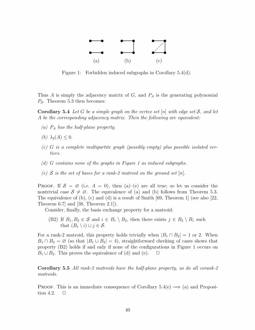
uu

uu

uu

uu

uu

uu

��

�

(a) (b) (c)

Figure 1: Forbidden induced subgraphs in Corollary 5.4(d).

Thus A is simply the adjacency matrix of G, and PA is the generating polynomialPS . Theorem 5.3 then becomes:

Corollary 5.4 Let G be a simple graph on the vertex set [n] with edge set S, and letA be the corresponding adjacency matrix. Then the following are equivalent:

(a) PA has the half-plane property.

(b) λ2(A) ≤ 0.

(c) G is a complete multipartite graph (possibly empty) plus possible isolated ver-tices.

(d) G contains none of the graphs in Figure 1 as induced subgraphs.

(e) S is the set of bases for a rank-2 matroid on the ground set [n].

Proof. If S = ∅ (i.e. A = 0), then (a)–(e) are all true; so let us consider thenontrivial case S 6= ∅. The equivalence of (a) and (b) follows from Theorem 5.3.The equivalence of (b), (c) and (d) is a result of Smith [69, Theorem 1] (see also [22,Theorem 6.7] and [38, Theorem 2.1]).

Consider, finally, the basis exchange property for a matroid:

(B2) If B1, B2 ∈ S and i ∈ B1 \ B2, then there exists j ∈ B2 \ B1 suchthat (B1 \ i) ∪ j ∈ S.

For a rank-2 matroid, this property holds trivially when |B1 ∩ B2| = 1 or 2. WhenB1 ∩ B2 = ∅ (so that |B1 ∪ B2| = 4), straightforward checking of cases shows thatproperty (B2) holds if and only if none of the configurations in Figure 1 occurs onB1 ∪B2. This proves the equivalence of (d) and (e). 2

Corollary 5.5 All rank-2 matroids have the half-plane property, as do all corank-2matroids.

Proof. This is an immediate consequence of Corollary 5.4(e) =⇒ (a) and Proposi-tion 4.2. 2

40

6 Necessary conditions I: Same-phase property

In this section and the next, we derive some necessary conditions that a homoge-neous polynomial with the half-plane property must satisfy.

Let us begin with a bit of motivation: Many “counting” results in combinatoricsfind a more natural context when they are generalized to allow nonnegative realweights, rather than restricting all weights to be 0 or 1. For example, the max-flow-min-cut theorem arises by generalizing Menger’s theorem in this way. Now, insome cases it is natural to go further and allow complex weights, but in some casesit is not. For example, in the Heilmann–Lieb theorem (see Section 10.1 below), thecomplex vertex weights {xi}i∈V are the main point, but it is essential that the edgeweights {λe}e∈E be nonnegative. Roughly speaking, it seems natural that variables inmultivariate polynomials be promoted to complex variables, but it is often necessarythat the coefficients in the polynomial be nonnegative real numbers.11

With this background in mind, we shall prove that if a homogeneous polynomialP (x) =

∑mamx

m has the half-plane property, then necessarily all the coefficientsam are nonnegative modulo an overall multiplicative phase factor.

Let us say that a pair of nonzero complex numbers a, b have the same phase ifa/b ∈ (0,∞). Obviously, having the same phase is an equivalence relation on C \ 0;and a collection {aα} of nonzero complex numbers all have the same phase if andonly if there exists θ ∈ R such that e−iθaα > 0 for all α. We say that a polynomialP (x) =

∑mamx

m has the same-phase property if all the nonzero coefficients am havethe same phase.

Theorem 6.1 Let P (x) =∑

mamx

m be a polynomial in n complex variables thatis homogeneous of degree r. If P has the half-plane property, then all the nonzerocoefficients am have the same phase.

Proof. The proof is by induction on n. If n = 1, we must have P (x) = arxr, so the

theorem is trivial. So assume n ≥ 2. Let M (≤ r) be the degree of xn in P (x), andlet us write

P (x) =M∑

k=0

xknPk(x1, . . . , xn−1) (6.1)

where of course

Pk(x1, . . . , xn−1) =1

k!(∂/∂xn)kP (x)

∣∣∣xn=0

. (6.2)

Clearly each coefficient of P corresponds to exactly one coefficient of exactly one Pk,and vice versa. Now, each Pk is a homogeneous polynomial (of degree r− k) in n− 1

11 Of course, given a polynomial expression, it is not always obvious which objects should beconsidered to be “variables” and which should be absorbed into the “coefficients”. So this admittedlyvague principle may in some cases be best understood backwards, i.e. as an injunction to treat as“variables” those objects that can naturally be made complex, and as “coefficients” those thatcannot.

41

variables; and by Corollary 2.10 it has the half-plane property. So, by the inductivehypothesis, all its nonzero coefficients have the same phase.

To complete the proof, we need only show that these phases are the same for allk. Applying Proposition 5.2 with x = (0, . . . , 0, 1) and y = (1, . . . , 1, 0), we get

px,y(ζ) = P (1, . . . , 1, ζ) =M∑

k=0

Pk(1, . . . , 1) ζk . (6.3)

Since px,y has only real nonpositive zeros, it can be written as px,y(ζ) = a∏M

k=1(ζ +ck) for some complex number a and nonnegative real numbers c1, c2, . . . , cM ; so itscoefficients Pk(1, . . . , 1) must all have the same phase. 2

Remark. It is easy to see that if P is homogeneous of degree 1, then P has thehalf-plane property if and only if all its nonzero coefficients have the same phase.

We can generalize Theorem 6.1 to a class of not-necessarily-homogeneous polyno-mials. Let us say that a polynomial P (x) =

∑mamx

m has definite parity if all thenonzero monomials have total degree of the same parity (i.e. am, am′ 6= 0 implies that|m| ≡ |m′| mod 2); this is equivalent to saying that the polynomial P is either evenor odd. We then have:

Theorem 6.2 Let P (x) =∑

mamx

m be a polynomial in n complex variables thathas definite parity and the half-plane property. Then all the nonzero coefficients am

have the same phase.

We begin the proof of Theorem 6.2 with a lemma:

Lemma 6.3 Let P and Q be polynomials in n complex variables, and suppose thatP + cQ has the same-phase property for all real c > 0. Then either

(a) all the nonzero coefficients of P and Q have the same phase

or else

(b) P and Q each have the same-phase property, and P = αQ for some nonzerocomplex number α.

Proof. Letting c → 0 (resp. c → +∞), we deduce that P (resp. Q) has the same-phase property. Let us write P (x) =

∑mamx

m and Q(x) =∑

mbmx

m. Now thereare two cases:

1) There is a multi-index m such that both am and bm are nonzero.

2) There is no such multi-index m.

42

In case 2, the fact that P+Q has the same-phase property implies that all the nonzerocoefficients of P and Q have the same phase.

In case 1, choose a multi-index m such that both am and bm are nonzero, anddefine rm = am/bm. If there is no multi-index n 6= m with either an or bn nonzero,then P (x) = amx

m and Q(x) = bmxm, which proves assertion (b) [with α = rm].

So assume that there is at least one such multi-index n, and consider an arbitraryone of them. Then, for all positive real numbers c, the complex numbers am + cbmand an + cbn have the same phase whenever they are both nonzero. If one of an andbn is zero, then by taking c → 0 or c → +∞ we can conclude (using the fact thatP and Q have the same-phase property) that am, bm and the nonzero member of{an, bn} all have the same phase, which implies (again using the fact that P and Qhave the same-phase property) that all the nonzero coefficients of P and Q have thesame phase. If, on the other hand, neither an nor bn is zero, let us define rn = an/bn.Then (rm + c)bm and (rn + c)bn have the same phase for all positive real numbersc /∈ {−rm,−rn}. Since bm and bn have the same phase, so do rm + c and rn + c. Sincethis is valid for all positive real c /∈ {−rm,−rn}, it follows that either rm and rn areboth real and positive, or else that rm = rn. If the former case holds for at least onemulti-index n for which an and bn are both nonzero, then all the nonzero coefficientsof P and Q have the same phase. If the latter case holds for all n for which at leastone of an and bn is nonzero, then P = αQ with α = rm. 2

Proof of Theorem 6.2. We proceed by induction on n. For n = 1, since P hasdefinite parity, its zeros are symmetric with respect to the origin. Since P also hasthe half-plane property, these zeros all lie symmetrically on the imaginary axis, sothat P (x) = axm

∏ki=1(x

2 + ci) for some complex number a, nonnegative integers mand k, and positive real numbers c1, c2, . . . , ck. This implies the same-phase propertyfor P .

For the induction step, suppose that P (x1, . . . , xn+1) has definite parity and thehalf-plane property. Let Pj(x) be the coefficient of xj

n+1 in P (x). Each Pj has definiteparity (this parity alternates with j) and has the half-plane property (by Corol-lary 2.10); so by the inductive hypothesis each Pj has the same-phase property. Wenow want to show that the nonzero coefficients of the various Pj all have the samephase.

Define jmin = min{j: Pj 6≡ 0} and jmax = max{j: Pj 6≡ 0}, and suppose thatjmin ≤ j < jmax. If Pj ≡ 0 (which of course can happen only for j > jmin), thenTheorem 3.4 states that Pj+1/Pj−1 is a strictly positive constant, so that the nonzerocoefficients of Pj−1 and Pj+1 have the same phase. If Pj 6≡ 0 and Pj+1 6≡ 0, thenTheorem 3.4 states that Pj+1/Pj is real-part-positive on Hn. Thus, by applyingTheorem 3.2 to the polynomial Pj(x)+yPj+1(x), where y is a new variable, we deducethat this polynomial has the half-plane property (in the variables x1, . . . , xn, y). Itfollows that, for any nonnegative real numbers c1, . . . , cn, the polynomial Pj(x) +(c1x1+. . .+cnxn)Pj+1(x) also has the half-plane property (in the variables x1, . . . , xn).

43

Since this latter polynomial has definite parity, by the inductive hypothesis it has thesame-phase property. Now apply Lemma 6.3 with P = Pj and Q(x) = x1Pj+1(x).In case (a), we conclude that all the nonzero coefficients of Pj and Pj+1 have thesame phase. In case (b), we conclude that Pj/Pj+1 = αx1 for some nonzero complexnumber α; but since Pj/Pj+1 is real-part-positive on Hn, α must be a positive realnumber, so we again conclude that all the nonzero coefficients of Pj and Pj+1 havethe same phase.

The foregoing observations show that the nonzero coefficients of all the Pj havethe same phase, and hence that P has the same-phase property. This completes theinduction step, and hence the proof. 2

Finally, let us take this opportunity to discuss the image of Hn under a homoge-neous polynomial P .

Proposition 6.4 Let P 6≡ 0 be a homogeneous polynomial of degree r ≥ 1 in ncomplex variables. If P does not have the half-plane property, then P (Hn) = C. If Pdoes have the half-plane property, then there exists θ ∈ R such that

P (Hn) = eiθHr =

eiθH if r = 1

C \ eiθ(−∞, 0] if r = 2

C \ 0 if r ≥ 3

(6.4)

[We apologize for the inconsistent notations Hn = H×. . .×H and Hr = {zr: z ∈ H}.We trust that this will not cause any confusion.]

Proof. Clearly P is nonconstant, so by the open mapping theorem, P (Hn) is open.By homogeneity, P (Hn) is a cone (i.e. invariant under multiplication by any λ > 0). IfP does not have the half-plane property, then P (Hn) ∋ 0; and an open cone containing0 must be all of C. Now suppose that P does have the half-plane property, so thatP (Hn) 6∋ 0. Then P (1, . . . , 1) 6= 0, so let θ = argP (1, . . . , 1). Since P (ζ, . . . , ζ) =ζrP (1, . . . , 1), it follows that P (ζ, . . . , ζ) covers the set eiθHr as ζ ranges over H .Therefore, P (Hn) ⊇ eiθHr.

Let us now prove the reverse containment. Suppose first that r = 1 and P (x) =∑ni=1 aixi. Then, as remarked above, P has the half-plane property if and only if all

the nonzero ai have the same phase, i.e. there exists θ ∈ R such that Re (e−iθai) ≥ 0for all i. But in this case P (Hn) = eiθH .

Suppose next that r = 2 and P (x) =∑n

i,j=1 ai,jxixj . By Theorem 6.1, there exists

θ ∈ R such that Re (e−iθaij) ≥ 0 for all i, j. But then Theorem 5.3(b) =⇒ (a) tellsus that P (Hn) = C \ eiθ(−∞, 0].

If r ≥ 3, the containment P (Hn) ⊆ C \ 0 is trivial. 2

44

Corollary 6.5 Fix N ≥ 2. Let {Ei}Ni=1 be disjoint finite sets, and for each i let

Pi be a polynomial of degree ri on the ground set Ei. [Note that Pi need not behomogeneous.] Suppose that P =

∑Ni=1 Pi, considered as a polynomial on the ground

set E =⋃N

i=1Ei, has the half-plane property. Then there is at most one index i withri ≥ 2 and Pi 6≡ 0.

Proof. Suppose that there are two such indices i, j. By setting xe = 0 for alle ∈ E\(Ei∪Ej), we can assume without loss of generality thatN = 2 and E = E1∪E2.Let us write x(1) = {xe}e∈E1 and x(2) = {xe}e∈E2, and let us define

Qλ(x) = λ−1P (λ1/r1x(1), λ1/r2x(2)) . (6.5)

Then Qλ has the half-plane property for all λ > 0; and by Hurwitz’s theorem, so does

limλ→+∞

Qλ(x) = P ♯1(x

(1)) + P ♯2(x

(2)) (6.6)

(recall from Section 2.2 that ♯ denotes leading part). So we can assume without lossof generalize that P1 and P2 are homogeneous. Applying Proposition 6.4, we concludethat there exist θ1, θ2 ∈ R such that Pi(H

Ei) ⊇ C \ eiθi(−∞, 0] for i = 1, 2. But thenwe can choose x(1) ∈ HE1 and x(2) ∈ HE2 so that P1(x

(1)) + P2(x(2)) = 0, showing

that P does not have the half-plane property. 2

Remark. We can also allow the sets Ei to be non-disjoint, provided that deg P1,degP2 ≥ |E1 ∩ E2| + 2: it suffices to fix xe ∈ H for e ∈ E1 ∩ E2 and then applyCorollary 6.5 in the remaining variables.

Let us conclude by mentioning an alternate proof of Theorem 6.1, which is morelengthy than the one given here but also more elementary (because it does not requireProposition 5.2). First one proves Theorem 6.1 in the multiaffine case by induction onr, deducing the same-phase property for P from that of its contractions P /i; the keytool here (ensuring the necessary “connectedness”) is Corollary 6.5. Then one uses aGrace–Walsh–Szego construction to reduce the case of a non-multiaffine polynomialto that of a multiaffine polynomial in a larger number of variables.

7 Necessary conditions II: Matroidal support

7.1 The exchangeability theorem

In this section we shall prove that if P 6≡ 0 is a homogeneous multiaffine polyno-mial with the half-plane property, then supp(P ) is necessarily the collection of basesof a matroid.

45

Theorem 7.1 Let P (x) =∑

S⊆E,|S|=r aSxS be a multiaffine homogeneous degree-r

polynomial (on the ground set E) that has the half-plane property and is not identicallyzero. Then there exists a rank-r matroid M on the ground set E such that supp(P ) =B(M).

When supp(P ) = B(M), we call the (obviously unique) matroid M the support ma-troid of P .

Indeed, with only a little more work we can prove a generalization to homogeneouspolynomials that are not necessarily multiaffine. First, a bit of notation: For multi-indices m and p, let m∧p be the multi-index defined by (m∧p)(e) = min[m(e),p(e)]for all e ∈ E. For e ∈ E, let us define the multi-index δe by

δe(f) =

{1 if f = e0 if f 6= e

(7.1)

If S is a set of multi-indices and m,p ∈ S, we say that m is exchangeable towardsp in S (and write “m → p in S”) to denote the following condition: for everye ∈ E such that m(e) > p(e), there exists an f ∈ E such that m(f) < p(f) andm − δe + δf ∈ S. This is an obvious generalization of the basis-exchange propertyfor matroids, to which it reduces if all the multi-indices are 0-1-valued.

Theorem 7.2 Let P (x) =∑

|m|=r amxm be a homogeneous degree-r polynomial (on

the ground set E) that has the half-plane property and is not identically zero. Then,for every m,m′ ∈ supp(P ), m is exchangeable towards m′ in supp(P ).

Clearly, by specializing Theorem 7.2 to the multiaffine case, we obtain Theorem 7.1.

Proof of Theorem 7.2. Since P is homogeneous, by Theorem 6.1 we may assumewithout loss of generality that am > 0 for all m ∈ supp(P ).

We proceed by induction on r. The cases r = 0 and r = 1 are trivial. Theinduction step fails when passing from r = 1 to r = 2, for reasons that will beexplained below. Therefore, we treat r = 2 as the base case of the induction, anddeduce it from Theorem 5.3 as follows: Let A = (aij)i,j∈E be the unique symmetricreal matrix such that P = PA. If the conclusion of the theorem fails, then thereexist m,m′ ∈ supp(P ) and e ∈ E with m(e) > m′(e) such that for any f ∈ E withm(f) < m′(f) we have m−δe+δf 6∈ supp(P ). Since r = 2 we may write m = δe+δg

and m′ = δb + δc (some of b, c, e, g may coincide). Since neither δg + δb nor δg + δc

is in supp(P ), we have abg = agb = acg = agc = 0. Let x = δe + ρδg for some ρ > 0,and let y = δb + δc. We see that

xTAy = (aeb + aec)/2 (7.2a)

yTAy = abc + (abb + acc)/2 > 0 (7.2b)

xTAx = ρaeg + (aee + ρ2agg)/2 > 0 (7.2c)

46

where aeg, abc > 0 since m,m′ ∈ supp(P )]. As ρ→ ∞, inequality (e) of Theorem 5.3eventually fails, so P does not have the half-plane property.

For the induction step, assume that r ≥ 3 and that the theorem holds for homo-geneous polynomials of degree r− 1. We shall employ an inner induction on n = |E|.The base case n = 1 is trivial. So assume the result for homogeneous polynomials ofdegree r and ground sets of size strictly less than n. Let P be a homogeneous poly-nomial of degree r on an n-element ground set E, and let m,m′ ∈ supp(P ). We shallshow that m → m′ in supp(P ), i.e. that for every e ∈ E such that m(e) > m′(e),there exists an f ∈ E such that m(f) < m′(f) and m − δe + δf ∈ supp(P ). Wedivide the argument into three cases:

1. There exists b ∈ E such that m(b) = m′(b) = 0.

2. There exists b ∈ E such that m(b) > 0 and m′(b) > 0.

3. For every b ∈ E, exactly one of m(b) > 0 or m′(b) > 0 holds.

Case 1. Suppose there exists an element b such that m(b) = m′(b) = 0. Thenconsider the polynomial P \b, which by Proposition 3.1 has the half-plane property.The ground set E \ b of P \b is strictly smaller than the ground set E of P , so thehypothesis of the inner induction applies. Both m and m′ are in the support of P \b, sowe have m → m′ in supp(P \b). Since supp(P \b) ⊆ supp(P ), it follows that m → m′

in supp(P ).

Case 2. Suppose there exists an element b such that m(b) > 0 and m′(b) > 0. Thenconsider the polynomial P /b, which by Proposition 3.1 has the half-plane property.This polynomial is homogeneous of degree r − 1, so the hypothesis of the outerinduction applies. Both m − δb and m′ − δb are in the support of P /b, so we have(m − δb) → (m′ − δb) in supp(P /b). Now let e ∈ E be such that m(e) > m′(e).Since (m − δb)(e) > (m′ − δb)(e), there is an f ∈ E with m(f) < m′(f) andm − δb − δe + δf ∈ supp(P /b). This implies that m− δe + δf ∈ supp(P ).

This argument shows that whenever p,q ∈ supp(P ) are such that p ∧ q > 0, wehave p → q in supp(P ). This fact will be used repeatedly in the remainder of theproof.

Case 3. Suppose that for every b ∈ E, exactly one of m(b) > 0 or m′(b) > 0 holds.We proceed in a series of steps:

(a) We claim that there is a multi-index k ∈ supp(P ) such that m ∧ k 6= 0 andm′ ∧ k 6= 0. Suppose not, and specialize xb = y if m(b) > 0 and xb = z if m′(b) > 0.The result is a polynomial of the form Ayr +Bzr for some numbers A,B > 0, whichhas the half-plane property. However, upon substituting the values y = B1/reiπ/2r

and z = A1/re−iπ/2r this polynomial vanishes, a contradiction (since r ≥ 2). Hencethere must exist a multi-index k ∈ supp(P ) as claimed.

(b) Next, we claim that there is a multi-index k′ ∈ supp(P ) such that |m∧k′| ≥ 2and |m′ ∧ k′| ≥ 1. (This is what fails in the case r = 2.) Perhaps the k found in step

47

(a) already satisfies this condition. If not, then |m ∧ k| = 1 and |m′ ∧ k| ≥ 2. Letb ∈ E be such that (m′ ∧ k)(b) > 0. Since k → m in supp(P ) [as shown in Case 2],there is a g ∈ E with k(g) < m(g) such that k′ = k − δb + δg ∈ supp(P ). This k′

meets the required conditions.(c) Next, we claim that there is a multi-index p ∈ supp(P ) such that |m∧p| ≥ 2

and |m′∧p| ≥ 1 and, moreover, for all b ∈ E such that m(b) > 0 we have p(b) ≤ m(b).To show this, we define

ν(p,m) =∑

b∈E: m(b)>0

max[0,p(b) − m(b)] (7.3)

and choose k′ ∈ supp(P ) as in step (b). If ν(k′,m) = 0 then we are done, so assumethat ν(k′,m) > 0. Let b ∈ E be such that m(b) > 0 and k′(b) > m(b). Since k′ → min supp(P ), there is a g ∈ E with k′(g) < m(g) such that p′ = k′−δb +δg ∈ supp(P ).We have ν(p′,m) < ν(k′,m) and |m∧p′| = |m∧k′| ≥ 2 and |m′∧p′| = |m′∧k′| ≥ 1.Repeating this argument inductively as required produces a multi-index p ∈ supp(P )satisfying the claim.

(d) Let e ∈ E be such that m(e) > m′(e), and consider two subcases:

(i) m(e) > p(e).

(ii) m(e) = p(e).

Subcase (i): If m(e) > p(e), then since m → p in supp(P ), there is an f ∈ Ewith m(f) < p(f) such that m − δe + δf ∈ supp(P ). Since m(f) < p(f) we musthave m(f) = 0, so that m(f) < m′(f).

Subcase (ii): Here m(e) = p(e) > 0 = m′(e). Therefore, since p → m′ insupp(P ), there is a g ∈ E with p(g) < m′(g) such that q = p − δe + δg ∈ supp(P ).Now we have m(e) > q(e) and m ∧ q > 0 and, moreover, for all b ∈ E such thatm(b) > 0 we have q(b) ≤ m(b). We may therefore repeat the argument of subcase(i) with q in place of p. 2

Remark. In step (a) of Case 3 we needed to invoke the same-phase property(Theorem 6.1) in order to ensure that A,B 6= 0. In the multiaffine case this isunnecessary, because only m and m′ contribute to A andB, so A,B 6= 0 is guaranteed;and this fact is enough to imply that Ayr +Bzr cannot have the half-plane property(by Corollary 6.5). In most other respects, however, the proof of Theorem 7.2 is notmuch more complicated than the proof for the multiaffine case.

Theorem 7.2 shows that the support of a homogeneous polynomial with the half-plane property satisfies a multi-analogue of the matroid basis-exchange axiom. Suchstructures were introduced by Bouchet and Cunningham [8] and are called “jumpsystems” (see also [49, 28]). For p ∈ ZE , let ‖p‖ =

∑e∈E |p(e)|. A nonempty subset

J ⊆ ZE is called a jump system (with ground set E) in case it satisfies the followingcondition:

48

(J) For any m,m′ ∈ J and k ∈ ZE such that ‖m − k‖ = 1 and ‖k − m′‖ =‖m − m′‖ − 1, either k ∈ J or there exists k′ ∈ J with ‖k − k′‖ = 1 and‖k′ − m′‖ = ‖m− m′‖ − 2.

A jump system J is said to have constant sum when |m| = |m′| for all m,m′ ∈ J .In this case, the condition defining a jump system is equivalent to requiring that forall m,m′ ∈ J , both m → m′ in J and (−m) → (−m′) in −J ≡ {−k: k ∈ J }.(The definition of exchangeability extends in the natural way from NE to ZE .)

Corollary 7.3 Let P 6≡ 0 be a homogeneous polynomial with the half-plane property.Then supp(P ) is a jump system with constant sum.

Proof. Since P is homogeneous, supp(P ) has constant sum. For any m,m′ ∈supp(P ), we have m → m′ in supp(P ) by Theorem 7.2. For each e ∈ E, let p(e) =dege P , and consider Q(x) = xpP (1/x). Since the open right half-plane is invariantunder the transformation z 7→ 1/z, Q is also a homogeneous polynomial with thehalf-plane property. Thus, by Theorem 7.2 again, (p − m) → (p − m′) in supp(Q).But this means that (−m) → (−m′) in − supp(P ). 2

A nonempty intersection of a jump system in ZE with the set {0, 1}E is knownas a delta-matroid , and is usually regarded as a set system (by identifying a set withits characteristic vector). When a delta-matroid is uniform (i.e. all sets have thesame size), then it is the collection of bases of a matroid (as is easily seen), so thatTheorem 7.1 is a special case of Corollary 7.3.

It is natural to wonder what can be said about the support of a polynomialP with the half-plane property, if one omits (or weakens) the assumption that Pis homogeneous. The fact that the same-phase property need not hold in this casecauses great complications; one might start by considering the subclass of polynomialsP that have the half-plane property and the same-phase property.

Question 7.4 If P is multiaffine and has the half-plane property, is supp(P ) a delta-matroid? What if P also has the same-phase property?

Question 7.5 Assume that P has the half-plane property and has definite parity (i.e.m,m′ ∈ supp(P ) implies that |m| ≡ |m′| mod 2). Is P then a jump system? (Recallfrom Theorem 6.2 that all such polynomials have the same-phase property.)

7.2 The weak half-plane property

Recall that a set system S (resp. a matroid M) is said to have the half-planeproperty if its generating polynomial PS (resp. its basis generating polynomial PB(M))does. Let us now say that a set system S (resp. a matroid M) has the weak half-plane property if there exists a polynomial P with the half-plane property for which

49

supp(P ) = S [resp. supp(P ) = B(M)]. This is obviously a weaker condition, since thenonzero coefficients of P need not all be equal. (By Theorem 6.1 they must, however,all have the same phase in the matroid case or, more generally, when the set systemis r-uniform.) Theorem 7.1 can then be rephrased as saying that if an r-uniform setsystem has the weak half-plane property, it is necessarily the collection of bases of amatroid. A central open question is the converse:

Question 7.6 Does every matroid M have the weak half-plane property? And if not,which ones do?

We shall soon show (Corollary 8.2) that all matroids representable over C have theweak half-plane property. But we are totally in the dark about matroids not rep-resentable over C, such as the Fano matroid F7 and its coextensions AG(3, 2) andS8 (which are representable only over fields of characteristic 2), the matroids T8, R9,S(5, 6, 12) and PG(2, 3) (which are representable only over fields of characteristic 3),or the Vamos and non-Pappus matroids (which are not representable over any field).

Remark. The weak half-plane property for an n-element matroid M is algorith-

mically testable in time cc2n+|B(M)|2

1 using cylindrical algebraic decomposition, and intime cn|B(M)| using more recent algorithms (see Section 2.6). But this is thoroughlyunfeasible in practice!

8 The determinant condition and 6√

1-matroids

8.1 The determinant condition

Let A be an r × n matrix with complex entries, and define

QA(x) = det (AXA∗) (8.1)

where X = diag(x1, . . . , xn) and ∗ denotes Hermitian conjugate. Clearly QA is mul-tiaffine and is homogeneous of degree r. We have the following straightforward gen-eralization of Theorem 1.1:

Theorem 8.1 Let A be an arbitrary complex r × n matrix, and define QA by (8.1).Then:

(a) QA has the half-plane property.

(b) QA(x) =∑

S ⊆ [n]

|S| = r

|det (A ↾ S)|2 xS , where A ↾ S denotes the (square) submatrix

of A using the columns indexed by the set S.

50

Proof. Note first that if rankA < r, then QA ≡ 0 and so trivially has the half-planeproperty; so let us assume that rankA = r. Then kerA∗ = 0, i.e. for every nonzeroψ ∈ Cr, we have A∗ψ 6= 0 in Cn. It follows that, for each ψ 6= 0, the quantity

ψ∗AXA∗ψ =n∑

i=1

|(A∗ψ)i|2 xi (8.2)

has strictly positive real part whenever Rexi > 0 for all i; so in particularAXA∗ψ 6= 0.Therefore the matrix AXA∗ is nonsingular, and so has a nonzero determinant.

The identity (b) is an immediate consequence of the Cauchy–Binet theorem.12

2

Remark. This proof is a direct generalization of the proof of Theorem 1.1, towhich it reduces if we take A to be the directed vertex-edge incidence matrix for anyorientation of G with the i0th row suppressed (here i0 is an arbitrary vertex of G).

Corollary 8.2 (a) Every matroid representable over C has the weak half-planeproperty.

(b) Let M be a rank-r matroid on n elements that can be represented over C by anr × n matrix A for which every r × r subdeterminant is either zero or else ofmodulus 1. Then M has the half-plane property.

Proof. (a) This is an immediate consequence of Theorem 8.1, since det (A ↾ S) 6= 0if and only if S ∈ B(M).

(b) Clearly |det (A ↾ S)|2 = 1 if S ∈ B(M) and 0 if S /∈ B(M). So, by The-orem 8.1(b) we have QA = PB(M), and by Theorem 8.1(a) QA has the half-planeproperty. 2

8.2 (F,G)-representability and 6√

1-matroids

Which matroids have the property of Corollary 8.2(b)? Certainly regular matroidsdo, as they can be represented over R (hence also over C) by a totally unimodular

12 The Cauchy–Binet theorem states that if A is an m × n matrix and B is an n × m matrix,where m ≤ n, then

det (AB) =∑

S ⊆ [n]|S| = m

(detA

[[m]|S

]) (det B

[S|[m]

]).

Here the sum runs over all m-element subsets S ⊆ [n] ≡ {1, 2, . . . , n}, A[[m]|S

]denotes the subma-

trix of A consisting of the columns from S (taken in order), and B[S|[m]

]denotes the submatrix of

B consisting of the rows from S (taken in order). See e.g. [50, pp. 128–129] for a proof.

51

r×n matrix A (i.e. one for which every square subdeterminant is either 0, +1 or −1).But, in fact, Corollary 8.2(b) applies to a larger class of matroids. Let us pose thesequestions more generally in the following context.

Let F be a field, let F ∗ be the multiplicative group F \0, and let G be a subgroupof F ∗. If A is a matrix over F , let us call A an (F,G)-matrix if every nonzerosubdeterminant of A lies in G (note, in particular, that every nonzero entry of A mustlie in G). And let us call A a weak (F,G)-matrix if every nonzero r×r subdeterminantof A lies in G, where A has rank r. Finally, let us call a matroid (F,G)-representableif it is representable over F by an (F,G)-matrix, and weakly (F,G)-representable ifit is representable over F by a weak (F,G)-matrix.

The concept of an (F,G)-representable matroid was introduced by Whittle [78]and studied further, under the hypothesis that −1 ∈ G, by Semple and Whittle [67]within the more general framework of partial fields.13 (We shall not need this moregeneral notion here, and we refer the reader to Semple and Whittle’s paper for adiscussion of it.) As these authors note, many important classes of matroids arespecial cases of (F,G)-representable matroids:

• F -representable matroids: G = F ∗.

• Regular matroids (also known as unimodular matroids [76]): Let F be any fieldof characteristic zero (e.g. F = Q,R or C), and let G = {−1, 1}.

• k-regular matroids [77, 78, 65, 56]: Let F be the field Q(α1, . . . , αk) obtained byextending the rationals by k algebraically independent transcendental elementsα1, . . . , αk, and let G be the set of all products of integer powers of differencesof distinct members of {0, 1, α1, . . . , αk}. Thus, 0-regular matroids are just theregular matroids; 1-regular matroids are also called near-regular. A matroid isω-regular if it is k-regular for some k.

• Dyadic matroids [77, 78]: Let F be any field of characteristic zero, and letG = {±2k: k ∈ Z}.

• Sixth-root-of-unity matroids ( 6√

1-matroid for short) [78]: Let F = C and G bethe multiplicative group Z6 of complex sixth roots of unity.

• Complex unimodular matroids: Let F = C and G be the multiplicative groupU(1) of complex numbers of modulus 1.

Most “naturally arising” examples of (F,G)-representability — including thoserelevant to this paper — have −1 ∈ G, and (as we shall see) the theory takes a simplerform under this hypothesis. Nevertheless, there is also some interesting theory thatcan be developed for the case −1 /∈ G: for example, in Appendix B, we characterize(F, {1})-representable matroids. We shall therefore comment briefly on which resultsseem to need −1 ∈ G and which do not.

13 These authors call it a (G, F )-matroid .

52

We begin with some easy lemmas:

Lemma 8.3 Let A be an (F,G)-matrix, and let B be an F -matrix.

(a) If B is obtained from A by a sequence of row or column deletions, then B is an(F,G)-matrix.

(b) If B is obtained from A by a sequence of row or column scalings by factors lyingin G, then B is an (F,G)-matrix.

(c) If −1 ∈ G, and B is obtained from A by a sequence of row or column inter-changes, then B is an (F,G)-matrix.

(d) If −1 ∈ G, and B is obtained from A by a sequence of pivots, then B is an(F,G)-matrix.

Proof. (a)–(c) are trivial. The proof of (d) is essentially identical to that of [67,Proposition 3.3]. 2

Lemma 8.4 The class of (F,G)-representable matroids is closed under deletion anddirect sum. Moreover, if −1 ∈ G, then the class is closed under contraction, duality,2-sum, and series and parallel connection.

Proof. The proof of the first sentence is straightforward. When −1 ∈ G, closureunder contraction follows from Lemma 8.3(d) by mimicking the argument of [55,Proposition 3.2.6]. As noted in [67, Proposition 4.2], closure under duality, 2-sum,and series and parallel connection follows by mimicking the standard arguments forfields that appear in [55, Theorem 2.2.8 and Proposition 7.1.21]. 2

It follows from the characterization of (F, {1})-representable matroids in Ap-pendix B that, when −1 6∈ G, the class of (F,G)-representable matroids need notbe closed under duality, 2-sum, series connection, or parallel connection. One ques-tion we have been unable to answer is the following:

Question 8.5 When −1 /∈ G, is the class of (F,G)-representable matroids alwaysclosed under contraction?

It follows from Theorem B.1 that the answer is affirmative when G = {1}, but we donot know whether this is so in general.

Our first nontrivial result is that weak (F,G)-representability is no more generalthan (F,G)-representability, at least when −1 ∈ G. We do not know whether thisresult holds without the assumption that −1 ∈ G.

53

Proposition 8.6 Let F be a field, and let G be a subgroup of the multiplicative groupF ∗ that contains −1. Let A be a rank-r m× n matrix over F that is a weak (F,G)-matrix. Then there is a rank-r r × n matrix B over F that is an (F,G)-matrix andfor which M [A] = M [B].

Proof. Let M = M [A]. Since A has rank r, we may delete m − r rows from Aleaving an r × n matrix A1 whose rows are linearly independent. Moreover, A1 is aweak (F,G)-matrix representing M . Now the following row and column operationsleave a determinant unchanged except for possibly multiplying it by −1:

(i) Interchanging two rows or two columns.

(ii) Adding a multiple of one row to another.

By operations (i) and (ii), A1 can be transformed into a matrix A2 of the form [D|Z]where D is a diagonal matrix all of whose diagonal entries are nonzero.

The matrix [D|Z] can be further transformed as follows. Let the top-left 2 × 2

submatrix of D be

[d1 00 d2

]. In [D|Z], perform the following operations:

(i) replace row 2 by row 2 plus d−11 times row 1;

(ii) replace row 1 by row 1 minus d1 times row 2;

(iii) replace row 2 by row 2 plus d−11 times row 1; and

(iv) interchange rows 1 and 2.

We now have, in the top-left corner, the submatrix

[1 00 −d1d2

]. We can repeat this

process until all the diagonal entries in D except possibly the last, dr, are ones. Theresulting matrix [D′|Z ′] is a weak (F,G)-matrix representing M . Since detD′ = dr,it follows that dr ∈ G. Thus, we can multiply the last row of [D′|Z ′] by d−1

r to obtaina weak (F,G)-matrix A3 representing M of the form [Ir|Y ].

We shall show next that A3 is an (F,G)-matrix. Let A′3 be a k × k submatrix of

A3 for some k with 1 ≤ k ≤ r− 1. The identity submatrix Ir of A3 has an r× (r− k)submatrix B1 each of whose columns contains all zeros in the rows of A3 that meet A′

3.Let A′′

3 be the submatrix of A3 consisting of those columns that meet some columnof A′

3. As A3 is a weak (F,G) matrix, the determinant of the matrix [B1|A′′3] is in

G. But the value of this determinant is ±detA′′3. Since −1 ∈ G, we deduce that

detA′′3 ∈ G. We conclude that A3 is indeed an (F,G)-matrix representing M . 2

Proposition 8.7 Let F be a field, and let G be a subgroup of F ∗ that contains −1.Let A be an (F,G)-matrix of rank r. Then there is an (F,G)-matrix B = [Ir|D]such that M [A] ≃M [B] and B is obtainable from A by a sequence of row or columninterchanges, pivots, and deletions of zero rows.

54

Proof. This follows from Lemma 8.3 by well-known arguments: see e.g. [67, Propo-sitions 3.5 and 4.1]. 2

If D is a matrix over F , let us denote by G(D♯) the simple bipartite graph whosevertices correspond to the rows and columns of D and whose edges correspond tothe nonzero entries of D [55, pp. 190, 194]. If H is a subgroup of F ∗, let us call DH-normalized if there exists a basis B for the cycle matroid of G(D♯) [i.e. a maximalspanning forest in G(D♯)] such that each entry in D corresponding to an edge in Blies in H .

We aim next to show that, given an (F,G)-matrix [Ir|D], we can perform a se-quence of row and column scalings by elements of G (thereby maintaining an (F,G)-matrix) to yield a matrix [Ir|D′] for which D′ is {1}-normalized. In fact, a muchstronger result is true:

Proposition 8.8 Let F be a field, and let G be a subgroup of F ∗. Consider a matrix[Ir|D] over F , in which all the nonzero elements of D lie in G. Let B = {b1, ..., bk} bea basis for the cycle matroid of G(D♯), and let {θ1, ..., θk} be elements of G. Then, by asequence of row and column scalings with scale factors in G, one can obtain from [Ir|D]a matrix [Ir|D′] in which the entry of D′ corresponding to bi is θi. In particular, everysubdeterminant of [Ir|D′] differs from the corresponding subdeterminant of [Ir|D] bya factor lying in G.

Proof. The proof of [55, Theorem 6.4.7] carries through with very minor modifica-tions to prove this proposition. 2

By definition, every 6√

1-matroid is a complex unimodular matroid. In fact, thetwo classes coincide:

Theorem 8.9 The classes of complex unimodular matroids and 6√

1-matroids areequal.

Proof. Evidently we need only prove that every complex unimodular matroid is a6√

1-matroid. By Propositions 8.7 and 8.8, we can represent any complex unimodularmatroid M by a matrix [Ir|D] over C in which all nonzero subdeterminants havemodulus one and in which D is {1}-normalized. The desired result then follows fromthe following two lemmas:

Lemma 8.10 Let D be a Z6-normalized matrix over C in which all nonzero subde-terminants have modulus one. Then all the nonzero entries of D are sixth roots ofunity.

Lemma 8.11 Let A be a square matrix over C, whose determinant has modulus 1,such that all nonzero entries are sixth roots of unity. Then det (A) is in fact a sixthroot of unity.

55

Let us prove these two lemmas in reverse order:

Proof of Lemma 8.11. Since det (A) is a linear combination, with coefficients ±1,of products of entries in A, it follows that det (A) belongs to the additive subgroupof C generated by the sixth roots of unity. In the complex plane, the elements ofthis subgroup are the vertices of a triangular lattice, which intersects the unit circleprecisely at the sixth roots of unity. 2

Proof of Lemma 8.10. Let B be a basis for the cycle matroid of G(D♯) suchthat each entry in D corresponding to an edge in B is a sixth root of unity. For eachnonzero entry d of D, let ed be the corresponding edge of G(D♯). If ed 6∈ B, thenadding ed to the subgraph of G(D♯) induced by B creates a unique cycle Cd, whoselength is some even integer 2k ≥ 4. Assume that there exists a nonzero entry d thatis not a sixth root of unity, and choose one for which k is minimal.

Let Dd be the k×k submatrix of D induced by the vertices of Cd. By construction,all the entries ofDd corresponding to edges in Cd\ed are sixth roots of unity. Moreover,if Dd contains any nonzero entry d′ besides those of Cd, then the corresponding edgeed′ of G(D♯) is a diagonal of Cd (note that this cannot occur in the minimal case2k = 4). It follows that |Cd′| < |Cd|, so the choice of d implies that d′ is a sixth rootof unity. Hence every nonzero entry of Dd except possibly d is a sixth root of unity.

Consider now the subgraph of G(D♯) induced by the vertices of Cd; among thecycles of this graph containing ed, choose a cycle C ′ of shortest length 2j ≤ 2k. LetD′

d be the j × j submatrix of Dd induced by the vertices of C ′. Then each row andcolumn of D′

d has exactly two nonzero entries corresponding to edges of C ′, and noother nonzero entries (by the minimality of C ′). Moreover, all the nonzero entries ofD′

d, except possibly d, are sixth roots of unity.Because each row and column of D′

d has exactly two nonzero entries, the expansionof det (D′

d) in permutations has exactly two nonzero terms, exactly one of whichcontains d. We conclude that det (D′

d) = a − bd where a and b are sixth roots ofunity. If det (D′

d) = 0, then d is a sixth root of unity. If det (D′d) has modulus 1, then

so does c ≡ a/b− d. Hence d is a complex number of modulus 1, which differs froma sixth root of unity (a/b) by another complex number (c) of modulus 1. It followsby simple geometry that d is a sixth root of unity. 2

It is well known that the regular matroids are characterized by the following listof equivalent properties [76]:

Theorem 8.12 The following are equivalent for a matroid M :

(a) M is (F, {±1})-representable for some field F of characteristic 0.

(a) M is weakly (F, {±1})-representable for some field F of characteristic 0.

(c) M is (Q, {±1})-representable.

56

(d) M is weakly (Q, {±1})-representable.

(e) M is representable over GF (2) and over at least one field of characteristic notequal to 2.

(f) M is representable over all fields.

More recently, Whittle [78] has given an analogous characterization of the 6√

1-matroids.Combining his (deep) results with our (comparatively elementary) Proposition 8.6 andTheorem 8.9, we obtain:

Theorem 8.13 (Whittle [78]) The following are equivalent for a matroid M :

(a) M is representable over GF (3) and at least one field of characteristic 2.

(b) M is representable over GF (3) and GF (4).

(c) M is representable over GF (3) and all fields GF (22k) for k integer.

(d) M is representable over all fields F that contain a root of the polynomial x2 −x+ 1. [In particular, M is representable over all fields GF (q) for which q is apower of 3, q is a square, or q ≡ 1 (mod 3).]

(e) M is representable over all fields GF (q) for which q 6≡ 2 (mod 3).

(f) M is (C,Z6)-representable.

(g) M is (C, U(1))-representable.

(h) M is weakly (C, U(1))-representable.

The excluded-minor characterization of regular matroids is well known [55, The-orems 13.1.1 and 13.1.2]:

Theorem 8.14 (Tutte)

(a) A binary matroid M is regular if and only if it has no minor isomorphic to F7

or F ∗7 .

(b) A matroid M is regular if and only if it has no minor isomorphic to U2,4, F7 orF ∗

7 .

More recently, Geelen, Gerards and Kapoor [29], as a corollary of their importantwork in determining the excluded minors for GF (4)-representable matroids, havegiven an analogous excluded-minor characterization of 6

√1-matroids:

Theorem 8.15 (Geelen–Gerards–Kapoor [29])

57

(a) A ternary matroid M is a 6√

1-matroid if and only if M has no minor isomorphicto F−

7 , (F−7 )∗ or P8.

(b) A matroid M is a 6√

1-matroid if and only if M has no minor isomorphic toU2,5, U3,5, F7, F

∗7 , F−

7 , (F−7 )∗ or P8.

It will be shown in Section 11 that none of F7, F∗7 , F−

7 , (F−7 )∗ and P8 has the half-

plane property. The next two corollaries come from combining this fact with the lasttwo theorems and Corollary 8.2:

Corollary 8.16 A binary matroid has the half-plane property if and only if it isregular.

Corollary 8.17 A ternary matroid has the half-plane property if and only if it is a6√

1-matroid.

To conclude this section, we remark that a much less elementary proof of Theo-rem 8.9 than the one given above comes from using Theorem 8.15(b) together withthe fact, which is not difficult to verify, that none of U2,5, U3,5, F7, F

∗7 , F−

7 , (F−7 )∗

and P8 is a complex unimodular matroid.

9 Uniform matroids

9.1 Half-plane property

The basis generating polynomial of the uniform matroid Ur,n is the elementarysymmetric polynomial

Er,n(x1, . . . , xn) =∑

1≤i1<i2<...<ir≤n

xi1xi2 · · ·xir (9.1)

(we set E0,n ≡ 1). We have the following fundamental result:

Theorem 9.1 Let 0 ≤ r ≤ n. Then:

(a) The elementary symmetric polynomial Er,n has the half-plane property.

(b) For r ≥ 1, the rational function Fr,n ≡ Er,n/Er−1,n is strictly real-part-positiveon Hn.

Note first that (a) implies (b), by Proposition 2.8(b) with λi = 1/(n− r + 1) forall i; and (b) implies (a), by Lemmas 2.7 and 2.6 and the fact (which is a special caseof Proposition 4.6) that the elementary symmetric polynomials Er,n with r < n areirreducible over any field. [Alternatively, the truth of (b) for all r ≥ 1 allows one to

58

prove (a) by induction on r, starting from E0,n ≡ 1 and using Lemma 2.6.] So we cantry to prove whichever half seems more convenient.

We have already given two proofs of Theorem 9.1(a): one based on nice principaltruncation (i.e. differentiation) starting from the easy case r = n (Proposition 4.13),and another based on nice principal cotruncation starting from the easy case r = 0(Proposition 4.16). We shall give a third proof in Section 10, based on showing thatUr,n is a nice transversal matroid (Corollary 10.3 and Example 10.1 following it).Let us here give two more proofs: one based on the Grace–Walsh–Szego coincidencetheorem, and one based on “series-parallel” identities for the rational functions Fr,n.

Fourth proof. We have Er,n(ξ, . . . , ξ) =(

nr

)ξr, which is manifestly novanishing for

ξ in the open right half-plane H . Since Er,n is symmetric and multiaffine, the Grace–Walsh–Szego coincidence theorem (Theorem 2.12) implies that Er,n is nonvanishingin Hn. 2

Fifth proof [25]. We shall prove (b) by induction on r. The case r = 1 is trivialfor all n. Now the following identities are easy to prove (for 1 ≤ r ≤ n):

Er,n(x) = Er,n−1(x6=i) + xiEr−1,n−1(x6=i) for any index i (9.2)

Er,n(x) =1

r

n∑

i=1

xiEr−1,n−1(x6=i) (9.3)

We therefore have

Fr,n(x) =1

r

n∑

i=1

xiEr−1,n−1(x6=i)

Er−1,n(x)(9.4a)

=1

r

n∑

i=1

xiEr−1,n−1(x6=i)

Er−1,n−1(x6=i) + xiEr−2,n−1(x6=i)(9.4b)

=1

r

n∑

i=1

xiFr−1,n−1(x6=i)

Fr−1,n−1(x6=i) + xi

(9.4c)

=1

r

n∑

i=1

(1

xi

+1

Fr−1,n−1(x6=i)

)−1

, (9.4d)

so that the strict real-part-positivity of Fr,n follows from that of Fr−1,n−1. 2

Remarks. 1. The computation (9.4) is really just (4.18) specialized to the caseof uniform matroids. So this is just an explicit version of the “nice cotruncation”proof of Proposition 4.16. Indeed, it was our analysis of the proof (9.4) that led usto abstract the idea of weighted principal cotruncation (Section 4.6).

2. The identity (9.4d) shows how Fr,n(x) can by synthesized as the admittance of a2-terminal series-parallel network whose elementary branch admittances are positive

59

multiples of the xi. To begin with, F1,n(x) = x1+· · ·+xn is the admittance of branchesx1, . . . , xn placed in parallel. Then Fr,n(x) is the admittance of n branches in parallel,the ith of which consists of admittances xi/r and Fr−1,n−1(x6=i)/r in series. [Of course,the admittance Fr−1,n−1(x6=i)/r is obtained from the network giving Fr−1,n−1(x6=i) bydividing each branch admittance by r.]

Now let Gr,n be the graph obtained by this construction: it contains approximatelynr edges, and each edge e is assigned an admittance αexi(e) for some positive constantαe and some index i(e). Then the spanning-tree polynomial TGr,n({xe}), with itsarguments specialized as xe → αexi(e), contains the polynomial Er,n(x1, . . . , xn) as afactor. In this way, Theorem 9.1(a) can be obtained as a corollary of Theorem 1.1.

More generally, one might try to prove the half-plane property for a polynomial Pby starting from the spanning-tree polynomial TG of a large graph G, specializing tofewer variables, and then extracting a factor. We do not know whether this methodcan be applied fruitfully in other cases.

9.2 Brown–Colbourn property

Let us now prove that for r < n, the uniform matroids Ur,n not only have thehalf-plane property but have the Brown–Colbourn property (which is stronger, byvirtue of Corollary 2.3).

Theorem 9.2 Let 0 ≤ r ≤ n − 1. Then the uniform matroid Ur,n has the “Brown–Colbourn property”, i.e. Re xi < −1/2 for all e implies PI(Ur,n)(x) 6= 0, where I(Ur,n) ={S ⊆ {1, . . . , n}: |S| ≤ r} is the collection of independent sets of Ur,n.

Proof. Since PI(Ur,n)(x1, . . . , xn) =∑r

k=0Ek,n(x1, . . . , xn) is manifestly symmetricand multiaffine, it follows from the Grace–Walsh–Szego coincidence theorem (Theo-rem 2.12) that it suffices to prove the Brown–Colbourn property for the univariatepolynomial

Ir,n(z) = PI(Ur,n)(z, . . . , z) =r∑

k=0

(n

k

)zk . (9.5)

A slightly sharper result than this is given in Proposition 9.3 below. 2

As preparation for the statement and proof of Proposition 9.3, let us note thatthe univariate reliability polynomial [cf. (1.7)] for the uniform matroid Ur,n is givenby

Relr,n(q) = (1 − q)nIr,n

( q

1 − q

)=

r∑

k=0

(n

k

)qk(1 − q)n−k (9.6)

and hence can be written as Relr,n(q) = (1 − q)n−rHr,n(q) with

Hr,n(q) =

r∑

k=0

(n

k

)qk(1 − q)r−k (9.7a)

60

=r∑

k=0

r−k∑

j=0

(−1)j

(n

k

)(r − k

j

)qj+k (9.7b)

=r∑

ℓ=0

qℓℓ∑

j=0

(−1)j

(n

ℓ− j

)(r − ℓ+ j

j

)(9.7c)

=

r∑

ℓ=0

(n− r − 1 + ℓ

ℓ

)qℓ (9.7d)

where we define(

n−r−1+ℓℓ

)= δℓ0 in case r = n.14

Proposition 9.3 (Wagner [73]) Let 0 ≤ r ≤ n − 1. Then all the zeros of Hr,n(q)lie in the annulus

1

n− r≤ |q| ≤ r

n− 1. (9.8)

In particular, all the zeros of Hr,n(q) lie in |q| ≤ 1, so that all the zeros of Ir,n(z) liein Re z ≥ −1/2.

Proof. The ratios of successive coefficients of Hr,n are λℓ =(

n−r−1+ℓℓ

)/(

n−r+ℓℓ+1

)=

(ℓ + 1)/(n − r + ℓ), which is nondecreasing as ℓ runs from 0 to r − 1. Thus, by theEnestrom–Kakeya theorem [51, Theorem 30.3 and Exercise 2] (see also [2]) it followsthat all the zeros of Hr,n lie in the annulus λ0 ≤ |q| ≤ λr−1. 2

10 The permanent condition: Transversal and co-

transversal matroids

10.1 Heilmann–Lieb theorem

We begin by recalling the Heilmann–Lieb [35] theorem on the zeros of matchingpolynomials. This theorem is most often quoted in its univariate version (see e.g. [48,Section 8.5]), but it is the multivariate result [35, Theorem 4.6 and Lemma 4.7] thatis truly fundamental.

Let G = (V,E) be a loopless graph, and let us define the matching polynomialwith edge weights {λe}e∈E and vertex weights {xi}i∈V :

MG(x;λ) =∑

matchings M

∏

e=ij∈M

λexixj . (10.1)

(Here e = ij means that the endpoints of e are i, j; if G is not simple, this is aslight abuse of notation but unlikely to cause any confusion. Note also that we could,

14 The binomial-coefficient identity used in the last step can be deduced from [32, eqns. (1.7) and(1.9)]. Alternatively, it is a specialization of [79, Exercise 4.15(a)] followed by [32, eqn. (1.7)].

61

if we wanted, restrict attention to simple graphs by replacing each set of paralleledges e1, . . . , ek with a single edge e′ of weight λe′ =

∑ki=1 λei

.) Define also thecomplementary matching polynomial

MG(x;λ) = xV MG(1/x;λ) (10.2)

where xV =∏

i∈V xi. If e = ij ∈ E, we have the fundamental recursion relation

MG(x;λ) = MG\e(x;λ) + λexixjMG−i−j(x;λ) (10.3)

or equivalentlyMG(x;λ) = MG\e(x;λ) + λeMG−i−j(x;λ) . (10.4)

Repeated application of (10.4) to all edges incident on a vertex i, followed by deletionof i, yields the key identity

MG(x;λ) = xiMG−i(x;λ) +∑

e ∼ i

e = ij

λeMG−i−j(x;λ) (10.5)

where e ∼ i denotes that e is incident on i. The Heilmann–Lieb theorem assertsthat if the edge weights are nonnegative, then the polynomials MG and MG have thehalf-plane property:

Theorem 10.1 (Heilmann and Lieb [35]) Let G = (V,E) be a loopless graph,and let {λe}e∈E be nonnegative edge weights. If Rexi > 0 for all i ∈ V , then

(a) MG(x;λ) 6= 0.

(b) For every i ∈ V , MG−i(x;λ) 6= 0.

(c) For every i ∈ V , ReMG(x;λ)

MG−i(x;λ)> 0.

(d) MG(x;λ) 6= 0.

Proof. We shall prove (a)–(c) by induction on |V |. The theorem is trivial if |V | = 0

or 1, since MG = 1 for |V | = 0 and MG(x1) = x1 for |V | = 1. So assume that (a)–(c)hold for all graphs with fewer than n vertices, and let |V | = n. Then (b) holds for Gbecause (a) holds for G− i. It then follows from (10.5) that

MG(x;λ)

MG−i(x;λ)= xi +

∑

e ∼ i

e = ij

λeMG−i−j(x;λ)

MG−i(x;λ). (10.6)

The right-hand side has positive real part because Rexi > 0, λe ≥ 0 andRe [MG−i−j(x;λ)/MG−i(x;λ)] > 0 by hypothesis (c) applied to G− i (using the fact

62

that the function z 7→ 1/z maps the right half-plane to itself). We conclude that (c)holds for G. Hence so does (a).

Finally, (d) follows from (a) by Proposition 4.2. 2

Remarks. 1. The same conclusion obviously holds [with a reversal of sign in (c)]if Re xi < 0 for all i. But the proof does not apply to other rotated half-planes, as weneed invariance under the function z 7→ 1/z. Indeed, the result for other half-planes

is false already for G = K2, which has MG(x1, x2;λ) = λ12 + x1x2.2. This proof is basically the same as that of Heilmann and Lieb [35, Lemma

4.7], but is slightly simpler and stronger: they prove (c) only for pairs (G′, G′ − i)belonging to their set EG.

3. How could one have guessed the key inductive hypothesis (c)? It suffices to

note, from (10.5), that ∂MG/∂xi = MG−i; and of course MG−i 6≡ 0 because it has

constant term 1. Therefore, by either Proposition 2.8(b) or Theorem 3.2(c), if MG

has the half-plane property, then necessarily hypothesis (c) must hold.4. Here is a simple alternate proof of Theorem 10.1(d), based on the concept of

multiaffine part (Proposition 4.17): The polynomial PG(x) =∏

e=ij∈E(1 + λexixj)

manifestly has the half-plane property whenever λe ≥ 0 for all e. But P ♭G (the

multiaffine part of PG) is precisely MG.

10.2 Application to transversal matroids

Now let us specialize the Heilmann–Lieb theorem to the case of a bipartite graphG = (V,E) with bipartition V = A ∪ B, setting xj = 1 for j ∈ B and consideringMG(x;λ) as a polynomial in {xi}i∈A. Then the restricted matching polynomial

MG(x;λ) =∑

matchings M

∏

e = ij ∈ M

i ∈ A

j ∈ B

λexi (10.7)

also has the half-plane property, provided that the edge weights are nonnegative.Consider now the transversal matroid M [G,A] with ground set A defined by the

bipartite graph G, in which a subset S ⊆ A is declared independent if it can bematched into B. Defining the weighted sum of such matchings,

c(S;λ) =∑

matchings M

V (M) ∩ A = S

∏

e∈M

λe , (10.8)

we find immediately that

MG(x;λ) =∑

S∈I(M [G,A])

c(S;λ) xS . (10.9)

63

So the restricted matching polynomial MG(x;λ), which has the half-plane property,is almost the independent-set generating polynomial for M [G,A]: the only troublecomes from the weights c(S;λ), which need not be equal. Likewise, the restrictedmaximum-matching polynomial

M ♯G(x;λ) =

∑

S ∈ I(M [G,A])

|S| = rank M [G, A]

c(S;λ) xS (10.10)

also has the half-plane property (by Proposition 2.2), and is almost the basis generat-ing polynomial for M [G,A], again modulo the problem of possibly unequal weights.

Note also that we may, if we wish, let G be the complete bipartite graph on thevertex set A ∪ B, since any undesired edges can always be given weight λe = 0.In particular, if we take A = [n], B = [r] and G = Kn,r, we have the followingpermanental analogue of Theorem 8.1 (see [53] for the definition and properties ofpermanents):

Theorem 10.2 Let Λ be an arbitrary nonnegative r × n matrix (r ≤ n), and definePΛ by

PΛ(x) = per(ΛX) (10.11)

where X = diag(x1, . . . , xn). Then:

(a) PΛ has the half-plane property.

(b) PΛ(x) =∑

S ⊆ [n]

|S| = r

per(Λ ↾ S) xS , where Λ ↾ S denotes the (square) submatrix of

Λ using the columns indexed by the set S.

Proof. Part (b) is an immediate consequence of the definition of the permanent ofa non-square matrix. Part (a) follows immediately from the Heilmann–Lieb theoremand the fact that

PΛ(x) = M ♯G(x;λ) = lim

α→∞α−rMG(αx;λ) (10.12)

with G = Kn,r. 2

Let us now call the pair (G,A) nice if there exists a collection {λe}e∈E of non-negative edge weights so that c(S;λ) has the same nonzero value for all bases S ofM [G,A]. And let us call the transversal matroid M nice if there exists a nice pair(G,A) such that M ≃M [G,A]. The foregoing results can be rephrased as follows:

Corollary 10.3

(a) Every transversal matroid has the weak half-plane property.

64

(b) Every nice transversal matroid has the half-plane property.

Unfortunately, Corollary 10.3(a) adds nothing to Corollary 8.2(a), since every transver-sal matroid is representable over all fields of sufficiently large cardinality, and hencein particular over C [55, Corollary 12.2.17]. But Corollary 10.3(b) is powerful, as weshall soon see.

Our next task should be to characterize nice pairs (G,A) and nice transversalmatroids M . Unfortunately, we are unable to do this in general, so we shall contentourselves with giving some examples of nice and non-nice transversal matroids. Asa preliminary, let us observe that the restriction of a nice pair (G,A) to any subsetA′ ⊆ A (and the same set B) yields a nice pair (G′, A′). In particular, any restrictionof a nice transversal matroid is a nice transversal matroid.

Let us also note that, to prove that a matroid M has the half-plane property, itsuffices by Proposition 4.2 to show that either M or its dual is a nice transversalmatroid. If M∗ is transversal, we say that M is cotransversal (also called a strictgammoid); if M∗ is nice transversal, we say that M is co-nice cotransversal .

10.3 Examples

In this subsection we give some examples of nice and non-nice transversal matroids.Sometimes, instead of specifying the pair (G,A), we shall find it more convenient tospecify the family A = {Aj}j∈B of subsets of A defined by i ∈ Aj if and only if ij ∈ E.The family A is called a presentation for M [G,A].

Example 10.1. Every uniform matroid Ur,n is nice. Indeed, it suffices to takethe obvious presentation, namely the one induced by the complete bipartite graphG = Kn,r with |A| = n and |B| = r, and to set λe = 1 for all e. 2

Example 10.2. Not all pairs (G,A) are nice. To see this, consider the bipartitegraph G shown in Figure 2, with A = {1, 2, 3, 4} and B = {x, y}. Then every2-element subset of A is matchable into B, and the weights are

c(12) = ad (10.13a)

c(13) = ae (10.13b)

c(14) = af (10.13c)

c(23) = be + cd (10.13d)

c(24) = bf (10.13e)

c(34) = cf (10.13f)

where for conciseness we have used the name of the edge e in place of λe. Supposethat all these subset weights are equal and nonzero. Then all the edge weights a, . . . , fmust be nonzero, and moreover we must have d = e = f and a = b = c. But thenc(23) = 2c(24), a contradiction. So this pair (G,A) is not nice. Note, nevertheless,

65

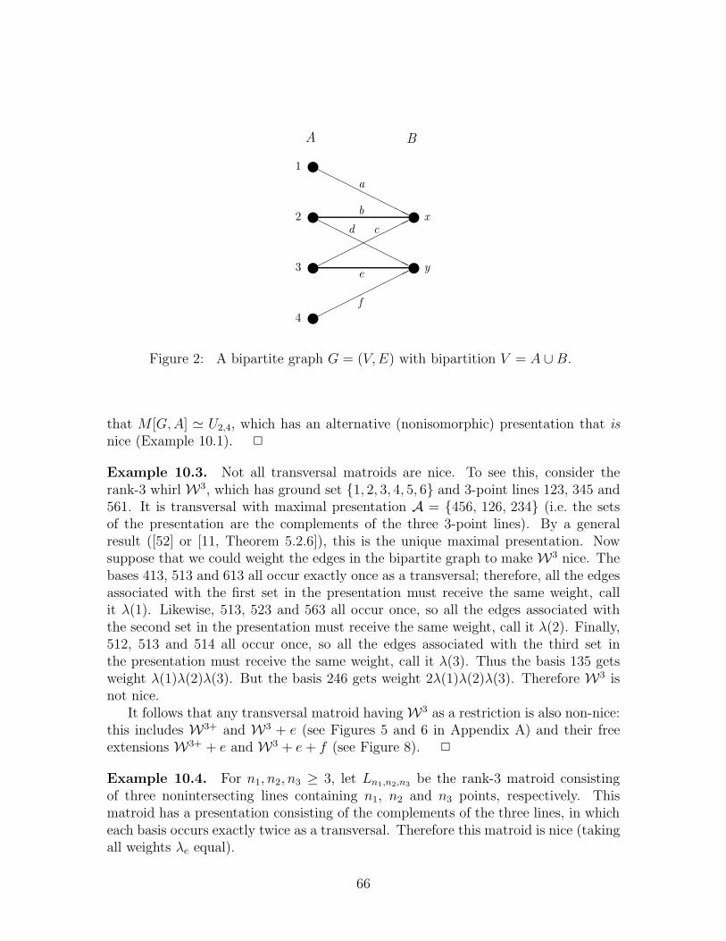
xxxx

xx

������������������HHHHHHHHH

HHHHHHHHH

4

3

2

1

y

x

A B

a

b

cd

e

f

Figure 2: A bipartite graph G = (V,E) with bipartition V = A ∪ B.

that M [G,A] ≃ U2,4, which has an alternative (nonisomorphic) presentation that isnice (Example 10.1). 2

Example 10.3. Not all transversal matroids are nice. To see this, consider therank-3 whirl W3, which has ground set {1, 2, 3, 4, 5, 6} and 3-point lines 123, 345 and561. It is transversal with maximal presentation A = {456, 126, 234} (i.e. the setsof the presentation are the complements of the three 3-point lines). By a generalresult ([52] or [11, Theorem 5.2.6]), this is the unique maximal presentation. Nowsuppose that we could weight the edges in the bipartite graph to make W3 nice. Thebases 413, 513 and 613 all occur exactly once as a transversal; therefore, all the edgesassociated with the first set in the presentation must receive the same weight, callit λ(1). Likewise, 513, 523 and 563 all occur once, so all the edges associated withthe second set in the presentation must receive the same weight, call it λ(2). Finally,512, 513 and 514 all occur once, so all the edges associated with the third set inthe presentation must receive the same weight, call it λ(3). Thus the basis 135 getsweight λ(1)λ(2)λ(3). But the basis 246 gets weight 2λ(1)λ(2)λ(3). Therefore W3 isnot nice.

It follows that any transversal matroid having W3 as a restriction is also non-nice:this includes W3+ and W3 + e (see Figures 5 and 6 in Appendix A) and their freeextensions W3+ + e and W3 + e+ f (see Figure 8). 2

Example 10.4. For n1, n2, n3 ≥ 3, let Ln1,n2,n3 be the rank-3 matroid consistingof three nonintersecting lines containing n1, n2 and n3 points, respectively. Thismatroid has a presentation consisting of the complements of the three lines, in whicheach basis occurs exactly twice as a transversal. Therefore this matroid is nice (takingall weights λe equal).

66

It follows that the matroids P6, S7, F−67 and P ′′′

7 (see Figures 4–7 in Appendix A)are nice, since they can be obtained by deleting elements from L3,3,3 or L4,3,3. 2

Example 10.5. More generally, let Ln1,n2,n3;n′ (with n1, n2, n3 ≥ 3 and n′ ≥ 0)be the rank-3 matroid consisting of three nonintersecting lines plus n′ freely addedpoints. Let us show that the smallest example with freely added points, namelyM = L3,3,3;1, is not nice:

Let the 3-point lines be abc, def and ghi, and call the freely added point 0. Then Mhas a presentation consisting of the complements of the three 3-point lines, i.e. A ={0abcdef, 0abcghi, 0defghi}. Indeed, this is the unique presentation.15 Now supposethat we could weight the edges in the bipartite graph to make M nice. For eachelement x of 0defghi, the basis abx occurs exactly twice as a transversal: as abx andas bax. This means that all the edges associated with the third set in the presentationmust receive the same weight, call it λ(3). By the same argument, all the edgesassociated with the second set in the presentation must receive the same weight λ(2),and all the edges associated with the first set in the presentation must receive thesame weight λ(1). Thus the basis abd gets weight 2λ(1)λ(2)λ(3). But the basis 0aegets weight 3λ(1)λ(2)λ(3). Therefore M is not nice. 2

Example 10.6. Let Ln1;n′ (with n1 ≥ 3 and n′ ≥ 1) be the rank-3 matroid con-sisting of one n1-point line plus n′ freely added points. By deletion from Ln1,3,3

(Example 10.4), we can conclude that Ln1;n′ is nice whenever n′ ≤ 4. Let us showthat the smallest remaining case, L3;5, is not nice:

L3;5 is transversal with unique maximal presentation A = {12345678, 12345678, 45678}.Let us denote the weights associated with the first (resp. second, third) set in the pre-sentation as λi (resp. λ′i, λ

′′i ). We shall use the combinations αij = λiλ

′j + λjλ

′i and

βij = λiλ′j − λjλ

′i.

For each pair of distinct elements i, j ∈ {1, 2, 3} and each x ∈ {4, 5, 6, 7, 8}, thebasis ijx occurs exactly twice as a transversal, always with the same two ways ofselecting i and j from the first two sets. Fixing i and j and letting x vary, weconclude that all the edges associated with the third set in the presentation mustreceive the same weight, which without loss of generality we may take equal to 1. Itthen follows that αij = 1 for all distinct i, j ∈ {1, 2, 3}.

For each i ∈ {1, 2, 3} and each triplet of distinct elements x, y, z ∈ {4, 5, 6, 7, 8},the bases ixy , ixz and iyz each occur exactly four times as transversals. Thus αix +αiy = 1, αix + αiz = 1 and αiy + αiz = 1. By comparing the first equation with

15 Proof. The presentation A is a maximal presentation, since adding an element to any setwill result in one of abc, def or ghi occurring as a transversal. By a general result ([52] or [11,Theorem 5.2.6]), this is the unique maximal presentation. The complements of the three sets in thepresentation are the three flats ghi, def and abc. Any other presentation must come from the maximalone by deleting elements from the sets in the presentation. This will increase the complements ofthese sets. But the complements of the sets in any presentation must be flats in M , and there areno flats other than E(M) that contain any one of abc, def or ghi. This proves the claim.

67

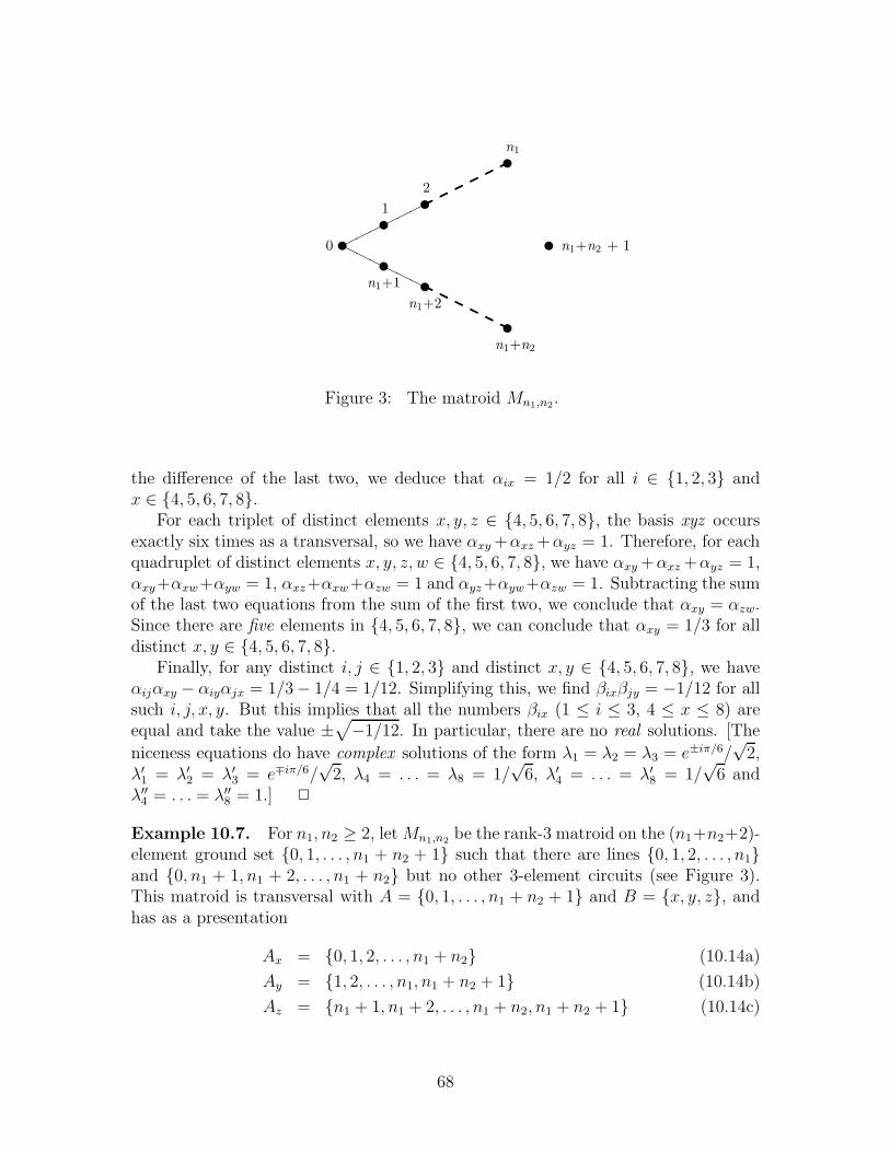
u u uu

u uu

u������

HHHHHH

0

1

2

n1

n1+1

n1+2

n1+n2

n1+n2 + 1

Figure 3: The matroid Mn1,n2.

the difference of the last two, we deduce that αix = 1/2 for all i ∈ {1, 2, 3} andx ∈ {4, 5, 6, 7, 8}.

For each triplet of distinct elements x, y, z ∈ {4, 5, 6, 7, 8}, the basis xyz occursexactly six times as a transversal, so we have αxy +αxz +αyz = 1. Therefore, for eachquadruplet of distinct elements x, y, z, w ∈ {4, 5, 6, 7, 8}, we have αxy +αxz +αyz = 1,αxy+αxw+αyw = 1, αxz+αxw+αzw = 1 and αyz+αyw+αzw = 1. Subtracting the sumof the last two equations from the sum of the first two, we conclude that αxy = αzw.Since there are five elements in {4, 5, 6, 7, 8}, we can conclude that αxy = 1/3 for alldistinct x, y ∈ {4, 5, 6, 7, 8}.

Finally, for any distinct i, j ∈ {1, 2, 3} and distinct x, y ∈ {4, 5, 6, 7, 8}, we haveαijαxy − αiyαjx = 1/3− 1/4 = 1/12. Simplifying this, we find βixβjy = −1/12 for allsuch i, j, x, y. But this implies that all the numbers βix (1 ≤ i ≤ 3, 4 ≤ x ≤ 8) areequal and take the value ±

√−1/12. In particular, there are no real solutions. [The

niceness equations do have complex solutions of the form λ1 = λ2 = λ3 = e±iπ/6/√

2,λ′1 = λ′2 = λ′3 = e∓iπ/6/

√2, λ4 = . . . = λ8 = 1/

√6, λ′4 = . . . = λ′8 = 1/

√6 and

λ′′4 = . . . = λ′′8 = 1.] 2

Example 10.7. For n1, n2 ≥ 2, let Mn1,n2 be the rank-3 matroid on the (n1+n2+2)-element ground set {0, 1, . . . , n1 + n2 + 1} such that there are lines {0, 1, 2, . . . , n1}and {0, n1 + 1, n1 + 2, . . . , n1 + n2} but no other 3-element circuits (see Figure 3).This matroid is transversal with A = {0, 1, . . . , n1 + n2 + 1} and B = {x, y, z}, andhas as a presentation

Ax = {0, 1, 2, . . . , n1 + n2} (10.14a)

Ay = {1, 2, . . . , n1, n1 + n2 + 1} (10.14b)

Az = {n1 + 1, n1 + 2, . . . , n1 + n2, n1 + n2 + 1} (10.14c)

68

Now put weights

λ0x = 1 (10.15a)

λix = 1/2 for 1 ≤ i ≤ n1 + n2 (10.15b)

λiy = 1 for all i ∈ Ay (10.15c)

λiz = 1 for all i ∈ Az (10.15d)

It is easily checked that c(S;λ) = 1 for every basis S of Mn1,n2. So this is a nicepresentation, and Mn1,n2 is a nice transversal matroid. In particular, Q6 ≃ M2,2,P6 ≃ M2,3 \ 0, Q7 ≃ M2,3, S7 ≃ M3,4 \ {0, 1} and P ′′′

7 ≃ M3,3 \ 0 are nice transversalmatroids. 2

Proposition 10.4 All matroids on a ground set of at most 6 elements have the half-plane property.

Proof. The half-plane property is preserved by direct sums (Proposition 4.4) and2-sums (Corollary 4.9). Therefore, we can restrict attention to 3-connected matroids.Since all rank-1 and rank-2 matroids have the half-plane property (Corollary 5.5), wecan restrict attention to matroids of rank ≥ 3. Finally, since the half-plane propertyis invariant under duality (Proposition 4.2), we can restrict attention to matroidsof rank ≤ ⌊n/2⌋, where n is the number of elements. So it suffices to consider 3-connected rank-3 matroids on 6 elements. All these matroids are shown in Figure 4(see Appendix A). The uniform matroid U3,6 has the half-plane property, as we haveshown many times (Section 9). The graphic matroid M(K4) and the whirl W3 are6√

1-matroids, hence have the half-plane property by Corollary 8.2(b). Finally, we havejust shown (Examples 10.4 and 10.7) that Q6 and P6 are nice transversal matroids,hence also have the half-plane property. 2

Example 10.8. The matroid F−57 (see Figure 6 in Appendix A) is transversal with

unique maximal presentation A = {2347, 4567, 1234567}. The bases 251, 351, 451 and751 all occur exactly once as a transversal; therefore, all the edges associated with thefirst set in the presentation must receive the same weight, call it λ(1). By symmetry,all the edges associated with the second set in the presentation must receive the sameweight, call it λ(2). But then 471 occurs twice as a tranversal, so it gets twice theweight that 251 gets. It follows that F−5

7 is not nice. 2

Example 10.9. The matroid (F−37 )∗ (see Figure 6) is transversal with unique max-

imal presentation A = {123, 147, 156, 345}. The bases 1465, 2465 and 3465 all occurexactly once as a transversal, so all the edges associated with the first set in thepresentation must receive the same weight, call it λ(1). By symmetry, all the edgesassociated with the second set in the presentation must receive the same weight, callit λ(2), and all the edges associated with the third set in the presentation must re-ceive the same weight, call it λ(3). Finally, the bases 1763, 1764 and 1765 all occur

69

exactly once as a transversal, so all the edges associated with the fourth set in thepresentation must receive the same weight, call it λ(4). But then 1345 occurs threetimes as a tranversal, so it gets three times the weight that 1456 gets. So (F−3

7 )∗ isnot nice. 2

Example 10.10. The matroid (F−47 )∗ (see Figure 6) is transversal with unique

maximal presentation A = {123, 147, 156, 1234567}. The bases 1456, 2456 and 3456all occur exactly twice as transversals, all with the same two ways of selecting 456from the last three sets in the presentation; so all the edges associated with the firstset in the presentation must receive the same weight, call it λ(1). By symmetry, allthe edges associated with the second set in the presentation must receive the sameweight, call it λ(2), and all the edges associated with the third set in the presentationmust receive the same weight, call it λ(3). Without loss of generality we can setλ(1) = λ(2) = λ(3) = 1. Let us denote the weights associated with the fourth set inthe presentation as λi (1 ≤ i ≤ 7). Bases then get weights as follows:

1245: λ1 + λ2 + λ4 + λ5

1345: λ1 + λ3 + λ4 + λ5

1246: λ1 + λ2 + λ4 + λ6

1346: λ1 + λ3 + λ4 + λ6

1276: λ1 + λ2 + λ7 + λ6

1376: λ1 + λ3 + λ7 + λ6

1234: λ2 + λ3

1475: λ4 + λ7

1562: λ5 + λ6

It follows from the first six bases that λ2 = λ3, λ5 = λ6 and λ4 = λ7. It then followsfrom the last three bases that λ2 = λ3 = . . . = λ7. But then we must have λ1 = −λ2.Therefore, the equations have no nonnegative solution, so (F−4

7 )∗ is not nice.Now consider the matroid (F−4

7 +e)∗ (see Figure 8) which is transversal with uniquemaximal presentation A = {123, 147, 156, 12345678, 12345678}. The first part of theargument just given for (F−4

7 )∗ carries over with slight modification to (F−47 +e)∗: the

bases 14568, 24568 and 34568 all occur exactly four times as transversals, all withthe same four ways of selecting 4568 from the last four sets in the presentation, soall the edges associated with the first set in the presentation must receive the sameweight λ(1); and by symmetry, all the edges associated with the second (resp. third)set in the presentation must receive the same weight λ(2) [resp. λ(3)]. Without lossof generality we can set λ(1) = λ(2) = λ(3) = 1. Let us denote the weights associatedwith the fourth (resp. fifth) set in the presentation as λi (resp. λ′i) for 1 ≤ i ≤ 8.Bases then get weights as follows:

14568: (λ5 + λ6)λ′8 + (λ′5 + λ′6)λ8

14578: (λ4 + λ7)λ′8 + (λ′4 + λ′7)λ8

12458: (λ1 + λ2 + λ4 + λ5)λ′8 + (λ′1 + λ′2 + λ′4 + λ′5)λ8

12678: (λ1 + λ2 + λ6 + λ7)λ′8 + (λ′1 + λ′2 + λ′6 + λ′7)λ8

70

All bases must get equal (and nonzero) weight. Thus, by comparing the sum of theweights of the first two bases with the sum of the weights of the last two bases, weconclude that λ1λ

′8 = λ2λ

′8 = λ′1λ8 = λ′2λ8 = 0 (since the weights are nonnegative).

But, by symmetry, the element 2 can be replaced by 3, 4, 5, 6 or 7. Hence λiλ′8 =

λ′iλ8 = 0 for 1 ≤ i ≤ 7, a contradiction. Therefore (F−47 + e)∗ is not nice. 2

Example 10.11. The matroid (W3 + e)∗ (see Figure 6) is transversal with uniquemaximal presentation A = {123, 345, 156, 1234567}. The bases 1467, 2467 and 3467all occur exactly once as a transversal; so all the edges associated with the first setin the presentation must receive the same weight, call it λ(1). By symmetry, all theedges associated with the second set in the presentation must receive the same weight,call it λ(2), and all the edges associated with the third set in the presentation mustreceive the same weight, call it λ(3). But then 1357 occurs twice as a transversal, soit gets twice the weight that 1467 does. So (W3 + e)∗ is not nice.

Now consider the matroid (W3 + e+ f)∗ (see Figure 8) which is transversal withunique maximal presentation A = {123, 345, 156, 12345678, 12345678}. The argu-ment just given for (W3 + e)∗ carries over verbatim to (W3 + e + f)∗ if we replaceeach basis abc7 by abc78 and we change “all occur exactly once as a transversal” to“all occur exactly twice as a transversal, all with the same two ways of selecting 78from the last two sets in the presentation”. It follows that (W3 + e+ f)∗ is not nice.2

Example 10.12. The matroid (F−57 )∗ (see Figure 6) is transversal with (non-

maximal) presentation A = {123, 156, 2467, 3457}, in which each basis occurs exactlytwice as a transversal. Therefore this matroid is nice (taking all weights λe equal).2

Example 10.13. The matroid (W3+)∗ (see Figure 5) is transversal with uniquemaximal presentation A = {156, 345, 1237, 1237}. The bases 1427, 5427 and 6427 alloccur exactly twice as transversals, all with the same two ways of selecting 27 fromthe last two sets in the presentation; so all the edges associated with the first set in thepresentation must receive the same weight, call it λ(1). By symmetry, all the edgesassociated with the second set in the presentation must receive the same weight, callit λ(2). Let us denote the weights associated with the third (resp. fourth) set in thepresentation as λi (resp. λ′i) for i = 1, 2, 3, 7. The bases 6417, 6427 and 6437 all occurexactly twice as transversals, from which we can conclude that λiλ

′7+λ

′iλ7 = α > 0 for

i = 1, 2, 3. But then 1357 gets weight 2λ(1)λ(2)α, while 1427 gets weight λ(1)λ(2)α.So (W3+)∗ is not nice.

Now consider the matroid (W3+ + e)∗ (see Figure 8) which is transversal withunique maximal presentation A = {156, 345, 1237, 1237, 12345678}. The argumentjust given for (W3+)∗ carries over verbatim to (W3+ + e)∗ if we replace each basis

71

abcd by abcd8. So (W3+ + e)∗ is not nice. 2

Example 10.14. The matroid (Q7)∗ (see Figure 5) is transversal with unique max-

imal presentation A = {123, 1456, 1456, 1234567}. The bases 1457, 2457 and 3457 alloccur exactly twice as transversals, all with the same two ways of selecting 457 fromthe last three sets in the presentation; so all the edges associated with the first setin the presentation must receive the same weight, which without loss of generalitywe take to be 1. Let us denote the weights associated with the second (resp. third,fourth) set in the presentation as λi (resp. λ′i, λ

′′i ). For each x ∈ {4, 5, 6}, the basis

21x7 occurs twice as a transversal (as 21x7 and 2x17); so λ1λ′x +λxλ

′1 takes the same

value α 6= 0 for x = 4, 5, 6. For each pair of distinct x, y ∈ {4, 5, 6}, the basis 1xy7occurs twice as a transversal (as 1xy7 and 1yx7); so λxλ

′y + λyλ

′x = α as well. Bases

then get weights as follows:

1452: α(λ′′1 + λ′′2 + λ′′4 + λ′′5)1453: α(λ′′1 + λ′′3 + λ′′4 + λ′′5)1463: α(λ′′1 + λ′′3 + λ′′4 + λ′′6)1563: α(λ′′1 + λ′′3 + λ′′5 + λ′′6)2143: α(λ′′2 + λ′′3)2456: α(λ′′4 + λ′′5 + λ′′6)

Comparing the first four bases, we conclude that λ′′2 = λ′′3 ≡ β and λ′′4 = λ′′5 = λ′′6 ≡ γ.But then λ′′1 + β + 2γ = 2β = 3γ, which implies that λ′′1 = −1

2γ. Therefore, the

equations have no nonnegative solution, so (Q7)∗ is not nice. 2

Example 10.15. The matroid P ′′7 (see Figure 7) is transversal with unique maximal

presentation A = {1267, 1345, 4567}. The bases 134, 234, 634 and 734 all occurexactly once as a transversal; therefore, all the edges associated with the first set inthe presentation must receive the same weight. Likewise, 216, 236, 246 and 256 (resp.134, 135, 136 and 137) all occur once, so all the edges associated with the second(resp. third) set in the presentation must receive the same weight. But then 147 getstwice the weight of 134. So P ′′

7 is not nice. 2

Example 10.16. The matroid (P ′7)

∗ (see Figure 7) is transversal with unique max-imal presentation A = {123, 156, 267, 345}. The bases 1574, 2574 and 3574 all occurexactly once as a transversal; therefore, all the edges associated with the first setin the presentation must receive the same weight. Analogous arguments using 2174,2574, 2674 (resp. 3524, 3564, 3574 or 2673, 2674, 2675) show that all the edges asso-ciated with the second (resp. third or fourth) set in the presentation must receive thesame weight. But then 1263 gets twice the weight of 1574. So (P ′

7)∗ is not nice.

Now consider the matroid (P ′7+e)∗ (see Figure 8) which is transversal with unique

maximal presentation A = {123, 156, 267, 345, 12345678}. The argument just given

72

for (P ′7)

∗ carries over verbatim to (P ′7 + e)∗ if we replace each basis abcd by abcd8. So

(P ′7 + e)∗ is not nice. 2

Example 10.17. The matroid (P ′′7 )∗ (see Figure 7) is transversal with (non-maximal)

presentation A = {123, 267, 345, 14567}, in which each basis occurs exactly twice asa transversal. Therefore (P ′′

7 )∗ is nice (taking all weights λe equal). 2

Example 10.18. More generally, for each n ≥ 1, letNn be the rank-(n+1) transver-sal matroid on the ground set {1, . . . , 2n+ 1} given by the presentation

A0 = {1, 2, 4, 6, 8, . . . , 2n− 4, 2n− 2, 2n, 2n+ 1} (10.16a)

Aj = {2j − 1, 2j, 2j + 1} for 1 ≤ j ≤ n (10.16b)

Geometrically, the dual of Nn consists of 3-point lines 123, 345, 567, . . . , (2n −1)(2n)(2n + 1) joined together in general position in rank n. Let S be a matchablesubset of {1, . . . , 2n + 1}. By using induction on n and considering separately thecases when S does and does not contain two consecutive members of {1, . . . , 2n+ 1},we can show (after some non-trivial work) that S arises from exactly two matchings.So, putting equal weights on all edges, we conclude that this is a nice presentation,and Nn is a nice transversal matroid. We have N1 ≃ U2,3, N2 ≃ U3,5 and N3 ≃ (P ′′

7 )∗.2

Example 10.19. The matroid (non-Pappus\1)∗ is transversal with maximal pre-sentation A = {247, 269, 348, 359, 456}. For each x ∈ {4, 5, 6}, the basis 7283x occursexactly once as a transversal, so all edges associated with the last set in the pre-sentation receive the same nonzero weight. For each y ∈ {3, 5, 9}, the basis 728y6occurs exactly once as a transversal, so all edges associated with the fourth set in thepresentation receive the same nonzero weight. For each z ∈ {2, 6, 9}, the basis 7z834occurs exactly once as a transversal, so all edges associated with the second set inthe presentation receive the same nonzero weight. Now consider the bases 29356 and26354. The first occurs exactly once as a transversal, while the second occurs exactlytwice (as 26354 and as 42356). Since the transversals 29356 and 26354 get the samenonzero weight, the transversal 42356 must get weight 0. Therefore the edge joiningthe element 4 to the first set in the presentation has weight 0. So we may delete 4from the first set and still have a presentation. This implies that {2, 7} contains acocircuit of (non-Pappus\1)∗ and hence contains a circuit of non-Pappus\1, which isfalse. So (non-Pappus\1)∗ is not nice. 2

We have written a Mathematica program nicetransversal.m to test a presen-tation A for niceness, using the Mathematica function Solve to solve the nicenessequations c(S;λ) = 1 for S ∈ B(M [A]). This program is available as part of the elec-tronic version of this paper at arXiv.org. However, because the niceness equationsare a polynomial system of degree r in a large number of variables, this programsometimes crashes for lack of memory or fails to complete even in several days ofCPU time.

73

10.4 Rank-3 transversal matroids

Let us now make a systematic study of the niceness of rank-3 transversal matroids.We begin by recalling Brylawski’s [13] algorithm for constructing transversal matroids.A principal transversal matroid (also called a fundamental transversal matroid) ofrank r is obtained by beginning with a distinguished basis B = {1, 2, . . . , r}, whichwe view geometrically as a simplex with vertices 1, 2, . . . , r, and adding elements asfollows: First one can add elements freely to the flat of rank 0 (i.e. add loops). Thenone can add elements freely to the flats of rank 1 (i.e. add elements parallel to thebasis elements). Then one can add elements freely to the lines spanned by two basiselements: such elements pick up the dependencies that are forced by virtue of theirlying on that line, but have no other dependencies. One continues this process byadding elements freely on the flats spanned by three basis elements, then by four basiselements, . . . and finally by r basis elements (the last are elements that are free inthe matroid).

Theorem 10.5 (Brylawski [13]) Every transversal matroid of rank r is a restric-tion of a principal transversal matroid of rank r, obtained by deleting some elementsof the original basis B.

Theorem 10.6 (Brylawski [13]) A principal transversal matroid has a unique pre-sentation, which consists of the r cocircuits that are the complements of the flatsspanned by the sets B \ i (1 ≤ i ≤ r).

Applying this construction in the case r = 3, we conclude that the most generalsimple rank-3 principal transversal matroid is Cn1,n2,n3;n′ with n1, n2, n3 ≥ 2 andn′ ≥ 0, defined as the rank-3 matroid on n1 + n2 + n3 + n′ − 3 elements consistingof consisting of three distinguished points (namely, the simplex vertices), three linesthat join pairs of these vertices and contain n1, n2 and n3 points, respectively, togetherwith n′ points freely added in the plane spanned by the vertices. All simple rank-3transversal matroids can then be obtained by deleting zero or more simplex verticesof Cn1,n2,n3;n′. By considering all the possibilities for simplex vertices to be deletedor not, and for the resulting lines to be nontrivial or trivial, we obtain the followingclasses of matroids:

1) Cn1,n2,n3;n′ with n1, n2, n3 ≥ 3 and n′ ≥ 0.

2) Dn1,n2;n′ with n1, n2 ≥ 3 and n′ ≥ 0, consisting of two intersecting lines contain-ing n1 and n2 points, respectively, together with n′ freely added points.

3) En1,n2,n3;n′ with n1, n2, n3 ≥ 3 and n′ ≥ 0, consisting of an n2-point line that ismet by nonintersecting lines with n1 and n3 points, respectively, together withn′ freely added points.

74

4) Fn1,n2,n3;n′ with n1, n2, n3 ≥ 3 and n′ ≥ 0, consisting of an intersecting pair oflines containing n1 and n2 points, respectively, and a third line containing n3

points that does not meet the first two, together with n′ freely added points.

5) Ln1,n2,n3;n′ with n1, n2, n3 ≥ 3 and n′ ≥ 0, consisting of three nonintersectinglines having n1, n2 and n3 points, respectively, together with n′ freely addedpoints.

6) Ln1,n2;n′ with n1, n2 ≥ 3 and n′ ≥ 0, consisting of two nonintersecting lineshaving n1 and n2 points, respectively, together with n′ freely added points.

7) Ln1;n′ with n1 ≥ 3 and n′ ≥ 1, consisting of one n1-point line together with n′

freely added points.

8) The uniform matroid U3,n′ with n′ ≥ 3, consisting of n′ points and no non-triviallines.

We can now determine which of these matroids are nice:Class 1. The smallest case C3,3,3;0 ≃ W3 is not nice (Example 10.3 above). And

since, starting from any larger matroid Cn1,n2,n3;n′ one can obtain C3,3,3;0 by deletingelements, it follows that all such matroids are non-nice.

Class 2. The matroid Dn1,n2;n′ is nice when n′ = 0 or 1 (Example 10.7). If n′ ≥ 2,the smallest case is D3,3;2 ≃ F−5

7 , which is not nice (Example 10.8). Therefore, allcases with n′ ≥ 2 are non-nice.

Class 3. The smallest case is E3,3,3;0 ≃ P ′′7 , which is not nice (Example 10.15).

Class 4. The smallest case is F3,3,3;0, which is not nice; the argument is similar tothat of Example 10.5 but is longer.

Class 5. The matroid Ln1,n2,n3;0 is nice (Example 10.4). All matroids Ln1,n2,n3;n′

with n′ ≥ 1 are not nice (Example 10.5).Class 6. By deletion from Ln1,n2,n3;0, we can conclude that Ln1,n2;n′ is nice when

n′ ≤ 2. The smallest remaining case is L3,3;3, which is not nice; the argument issimilar to that of Example 10.5 but is longer.

Class 7. By deletion from Ln1,n2,n3;0, we can conclude that Ln1;n′ is nice whenn′ ≤ 4. The smallest remaining case is L3;5, which is not nice (Example 10.6).

Class 8. All uniform matroids are nice (Example 10.1).

10.5 A wild speculation

Not all transversal matroids are nice; but this means only that our method forproving the half-plane property fails in these cases, not that the half-plane propertyitself fails. Indeed, we do not know a single example of a transversal matroid thatfails the half-plane property. Moreover, we have conducted extensive numerical exper-iments (see Section 12) on the rank-3 transversal matroids discussed in the previous

75

subsection, and it seems plausible that all rank-3 transversal matroids have the half-plane property. Might all transversal matroids (and hence all gammoids) have thehalf-plane property? Unfortunately, we have no idea how to prove this.

Remark. The strongly base-orderable matroids [40, 11] form a minor-closed classthat contains all the transversal matroids; so one might entertain the even strongerconjecture that “every strongly base-orderable matroid has the half-plane property”.However, this conjecture is false, since the matroid F−3

7 is strongly base-orderablebut does not have the half-plane property (Example 11.7 below). To see that F−3

7

is strongly base-orderable, it suffices to note that a rank-3 matroid is strongly base-orderable ⇐⇒ it is base-orderable ⇐⇒ it has no restriction isomorphic to M(K4)[40].

11 Counterexamples

In this section we use Proposition 5.2(a) =⇒ (b) to show that certain polynomialsdo not have the half-plane property.

Example 11.1. Consider the Fano matroid F7 with the ground set numbered asshown in Figure 6 (see Appendix A). Its basis set B(F7) consists of all 3-elementsubsets of [7] except {1, 2, 3}, {3, 4, 5}, {1, 5, 6}, {1, 4, 7}, {2, 5, 7}, {3, 6, 7} and{2, 4, 6}. Let P be the basis generating polynomial PB(F7). If we take x = χ{1,2,4,5}

and y = χ{3,6,7} (where χA denotes characteristic function of the set A), we obtain

px,y(ζ) = 4ζ3+12ζ2 +12ζ , whose roots are ζ = 0, (−3±√

3 i)/2. So the Fano matroiddoes not possess the half-plane property.

In fact, the Fano matroid is minor-minimal for failing to have the half-plane prop-erty. Indeed, it follows from Proposition 10.4 that every 7-element matroid lackingthe half-plane property is minor-minimal. 2

Example 11.2. Consider next the non-Fano matroid F−7 (Figure 6), which is ob-

tained from F7 by relaxing the circuit-hyperplane {2, 4, 6}, so that B(F−7 ) = B(F7) ∪

{{2, 4, 6}}. With the same choices of x and y, we obtain px,y(ζ) = 4ζ3 + 13ζ2 + 12ζ ,whose roots are ζ = 0, (−13 ±

√23 i)/8. So the non-Fano matroid does not possess

the half-plane property either; and, as noted above, it is minor-minimal. 2

Example 11.3. Consider next the matroid F−−7 obtained from F−

7 by relaxing{1, 4, 7} (Figure 6). Choosing x = χ{1,4,7} and y = χ{2,3,5,6}, we obtain px,y(ζ) =ζ3 +12ζ2 +13ζ+4, whose roots are ζ ≈ −10.834170 and ζ ≈ −0.582915±0.171501 i.So F−−

7 does not possess the half-plane property either; and, as noted above, it isminor-minimal. 2

Example 11.4. A similar approach shows that the matroid M(K4) + e obtainedfrom F−−

7 by relaxing {3, 4, 5} (Figure 6) also fails to possess the half-plane property.

76

But we can no longer choose x and y to be characteristic functions. Instead, let ustake a unified approach to F7, F

−7 , F−−

7 and M(K4) + e that gives additional insightinto why the half-plane property fails.

Let us start with the graphic matroid M(K4), which of course does have thehalf-plane property (by Theorem 1.1). Let K4 have vertex set {1, 2, 3, 4}. If we takex = χ{12,13,14} and y = χ{23,24,34}, we find px,y(ζ) ≡ PB(M(K4))(ζx+y) = ζ(ζ+3)2, whichhas a double root at ζ = −3. So M(K4) satisfies the condition of Proposition 5.2(b),but “just barely”: by suitable perturbations we may be able to split the double rootinto a pair of complex-conjugate roots, thereby proving the failure of the half-planeproperty for the perturbed matroid.

In the matroids F7 et al ., let us consider 4 to be the “new element”, i.e. F7 \ 4 ≃F−

7 \ 4 ≃ . . . ≃M(K4). Then the above choice of x and y corresponds to taking y tobe the characteristic function of a 3-point line in M(K4) and x to be the characteristicfunction of the complementary set, e.g. x = χ{1,2,5} and y = χ{3,6,7}. So let us perturbthis slightly, by taking x = χ{1,2,5} + ǫχ{4} and y = χ{3,6,7} + aǫχ{4} with ǫ, a ≥ 0.(Our previous choices for F7 and F−

7 correspond to ǫ = 1 and a = 0.) We then have:

F7: px,y(ζ) = (1 + 3ǫ)ζ3 + [6 + (6 + 3a)ǫ]ζ2 + [9 + (3 + 6a)ǫ]ζ + 3aǫ

Roots ζ = −(a/3)ǫ + O(ǫ3/2) and ζ = −3 ± 2√a− 3 ǫ1/2 + O(ǫ).

F−7 : px,y(ζ) = (1 + 3ǫ)ζ3 + [6 + (7 + 3a)ǫ]ζ2 + [9 + (3 + 7a)ǫ]ζ + 3aǫ

Roots ζ = −(a/3)ǫ + O(ǫ3/2) and ζ = −3 ±√

3(a− 3) ǫ1/2 + O(ǫ).

F−−7 : px,y(ζ) = (1 + 3ǫ)ζ3 + [6 + (8 + 3a)ǫ]ζ2 + [9 + (3 + 8a)ǫ]ζ + 3aǫ

Roots ζ = −(a/3)ǫ + O(ǫ3/2) and ζ = −3 ±√

2(a− 3) ǫ1/2 + O(ǫ).

M(K4) + e: px,y(ζ) = (1 + 3ǫ)ζ3 + [6 + (9 + 3a)ǫ]ζ2 + [9 + (3 + 9a)ǫ]ζ + 3aǫ

Roots ζ = −(a/3)ǫ + O(ǫ3/2) and ζ = −3 ±√a− 3 ǫ1/2 + O(ǫ).

So any choice of a ∈ [0, 3) will yield nonreal roots for small ǫ > 0 for all four matroids.Let us conclude this example by remarking that a second (nonisomorphic) choice of

x, y in M(K4) also yields a double root: for x = χ{12,34} and y = χ{13,14,23,24}, we findpx,y(ζ) = 4(ζ + 1)2, which has a double root at ζ = −1. An analogous perturbationof this choice also yields nonreal roots for F7 et al ., provided that a ∈ [0, 1). 2

Example 11.5. Consider the polynomial

Pµ(z1, . . . , z7) = PB(F7)(z) + µz2z4z6 . (11.1)

For µ = 0 (resp. µ = 1) this is the basis generating polynomial of F7 (resp. F−7 ). For

µ = 4 it is the polynomial QA(z) = det (AZAT) obtained from Z = diag(z1, . . . , z7)and the matrix

A =

1 1 0 0 0 1 10 1 1 1 0 0 10 0 0 1 1 1 1

, (11.2)

77

which represents F−7 over any field of characteristic 6= 2 (in particular, over C); by

Theorem 8.1, QA has the half-plane property. As in Example 11.4, let us choosex = χ{1,2,5} + ǫχ{4} and y = χ{3,6,7} + aǫχ{4} with ǫ, a ≥ 0. We then obtain px,y(ζ) =(1 + 3ǫ)ζ3 + [6 + (6 + µ + 3a)ǫ]ζ2 + [9 + (3 + 6a + µa)ǫ]ζ + 3aǫ, whose roots areζ = −(a/3)ǫ + O(ǫ3/2) and ζ = −3±

√(4 − µ)(a− 3) ǫ1/2 + O(ǫ). So, if −∞ < µ < 4

(resp. µ > 4), then any choice 0 ≤ a < 3 (resp. a > 3) will yield nonreal roots forsmall ǫ > 0. So Pµ has the half-plane property only for µ = 4! 2

Example 11.6. Consider, more generally, the polynomial

Pµ,ν,ρ(z1, . . . , z7) = PB(F7)(z) + µz2z4z6 + νz1z4z7 + ρz3z4z5 . (11.3)

For (µ, ν, ρ) = (0, 0, 0) this is PB(F7); for (µ, ν, ρ) = (1, 0, 0) it is PB(F−7 ); for (µ, ν, ρ) =

(1, 1, 0) it is PB(F−−7 ); for (µ, ν, ρ) = (1, 1, 1) it is PB(M(K4)+e).

Some cases of the polynomial Pµ,ν,ρ are of the form QA(z) = det (AZA∗) [whereZ = diag(z1, . . . , z7)] for a suitable complex matrix A, and thus have the half-planeproperty by Theorem 8.1. Consider, for instance, the matrix

A =

1 1 0 a 0 1 10 1 1 1 0 0 10 0 0 1 1 b b

(11.4)

For a = 0 and b = eiθ, we have QA = Pµ,ν,ρ with (µ, ν, ρ) = (2 + 2 cos θ, 2 − 2 cos θ, 0)[that is, µ, ν ≥ 0 with µ + ν = 4 and ρ = 0].16 For a = e±πi/3 and b = 1, we haveQA = Pµ,ν,ρ with (µ, ν, ρ) = (3, 0, 1); and for a = e±πi/3 and b = e∓2πi/3, we haveQA = Pµ,ν,ρ with (µ, ν, ρ) = (0, 3, 1). Moreover, by appropriately permuting columnsof the matrix A (without permuting the column labels), the triplet (µ, ν, ρ) can bepermuted at will.17 We do not know whether any additional cases of Pµ,ν,ρ can beobtained from a determinant.

For 0 ≤ µ, ν, ρ ≤ 2 with µ + ν + ρ = 4, the polynomial Pµ,ν,ρ arises from theprincipal extension of F7 \ 4 ≃M(K4) by the new element 4 with weights

λ2 = λ6 = 1 − µ/2 (11.5a)

λ1 = λ7 = 1 − ν/2 (11.5b)

λ3 = λ5 = 1 − ρ/2 (11.5c)

and thus has the half-plane property by Proposition 4.11.Finally, as in Example 11.5, let us choose x = χ{1,2,5} + ǫχ{4} and y = χ{3,6,7} +

aǫχ{4} with ǫ, a ≥ 0. We then obtain the same px,y as in Example 11.5, except that

16 We remark that the matrix A represents F−−7 over any field of at least four elements, provided

that a = 0 and b /∈ {0, 1,−1}.17 This is because there are automorphisms of F7 that realize an arbitrary permutation of the

lines 246, 147 and 345.

78

µ is replaced by µ + ν + ρ. So we obtain nonreal roots for small ǫ > 0 wheneverµ + ν + ρ 6= 4. It follows (using also Theorem 6.1) that Pµ,ν,ρ has the half-planeproperty only when µ, ν, ρ ≥ 0 with µ + ν + ρ = 4. But we do not know whetherthese necessary conditions are sufficient. 2

Example 11.7. Consider the matroid F−37 obtained from F−

7 by relaxing the circuit-hyperplanes {2, 5, 7} and {3, 6, 7} (Figure 6). Let us take x = χ{1,4,5} + ǫχ{2} andy = χ{3,6,7}. Then px,y(ζ) = (1 + 3ǫ)ζ3 + (6 + 8ǫ)ζ2 + (9 + 3ǫ)ζ + 1, which has nonrealroots whenever 0.090685 ∼< ǫ ∼< 0.494485. So F−3

7 does not have the half-planeproperty; and, as noted above, it is minor-minimal.

Note, finally, that F−37 is a relaxation of P7, which is a 6

√1-matroid and hence has

the half-plane property (see Section 8). So relaxation does not in general preservethe half-plane property. 2

Example 11.8. Consider the rank-4 matroid P8 represented over any field of char-acteristic 6= 2 by the matrix

1 0 0 0 0 1 1 20 1 0 0 1 0 1 10 0 1 0 1 1 0 10 0 0 1 2 1 1 0

(11.6)

Its basis set B(P8) consists of all 4-element subsets of [8] except {1, 2, 3, 8}, {1, 2, 4, 7},{1, 3, 4, 6}, {2, 3, 4, 5}, {1, 4, 5, 8}, {2, 3, 6, 7}, {1, 5, 6, 7}, {2, 5, 6, 8}, {3, 5, 7, 8} and{4, 6, 7, 8}. If we take x = χ{1,4,5,8} and y = χ{2,3,6,7}, we obtain px,y(ζ) = 16ζ3+28ζ2+

16ζ , whose roots are ζ = 0, (−7 ±√

15 i)/8. So P8 does not possess the half-planeproperty. Moreover, it is minor-minimal, since all the single-element contractions(resp. deletions) of P8 are isomorphic to P7 (resp. P ∗

7 ), which are 6√

1-matroids andhence have the half-plane property.

Observe now that {1, 4, 5, 8} and {2, 3, 6, 7} form the unique pair of disjoint circuit-hyperplanes in P8. Let us denote by P ′

8 the matroid obtained from P8 by relaxingone of these circuit-hyperplanes (say, {1, 4, 5, 8}), and by P ′′

8 the matroid obtainedby relaxing both of them. Let us make the same choices of x and y as for P8.Then, for P ′

8 one has px,y(ζ) = ζ4 + 16ζ3 + 28ζ2 + 16ζ , whose roots are ζ = 0and ζ ≈ −14.093869,−0.953065 ± 0.476353 i. And for P ′′

8 one has px,y(ζ) = ζ4 +16ζ3 + 28ζ2 + 16ζ + 1, whose roots are ζ ≈ −14.093459,−0.070955,−0.917793 ±0.397059 i. So neither P ′

8 nor P ′′8 possesses the half-plane property. We suspect (but

are unable to prove) they are minor-minimal: all the single-element contractions(resp. deletions) of P ′

8 are isomorphic to P7 or P ′7 (resp. P ∗

7 or (P ′7)

∗), and all thesingle-element contractions (resp. deletions) of P ′′

8 are isomorphic to P ′7 (resp. (P ′

7)∗);

and our numerical results (Section 12) suggest that P ′7 (and hence also its dual) has

the half-plane property. 2

Example 11.9. Consider the Pappus and non-Pappus matroids (Figure 9 in Ap-pendix A). Take x = 2χ{1} + χ{3,4,6,7} + ǫχ{9} and y = χ{2,5,8}. We then have:

79

Pappus: px,y(ζ) = (16 + 14ǫ)ζ3 + (33 + 15ǫ)ζ2 + (18 + 3ǫ)ζ + 1

Roots ζ = − 116

+O(ǫ) and ζ = −1 ± (i√

2/15)ǫ1/2 +O(ǫ).

non-Pappus: px,y(ζ) = (16 + 14ǫ)ζ3 + (33 + 16ǫ)ζ2 + (18 + 3ǫ)ζ + 1

Roots ζ = − 116

+O(ǫ) and ζ = −1 ± (i/√

15)ǫ1/2 + O(ǫ).

So the Pappus and non-Pappus matroids do not have the half-plane property. We donot know whether they are minor-minimal; but we suspect that they are, since ournumerical experiments (Section 12) suggest that their two non-isomorphic deletions,non-Pappus\1 and Pappus\e ≃ non-Pappus\9, do have the half-plane property. (Ofcourse, all their contractions are rank-2 and hence have the half-plane property.) 2

It is worth noting that non-Pappus\9 is “borderline” for the half-plane property inthe same sense that M(K4) is (Example 11.4), i.e. px,y(ζ) has a double root at ζ = −1for a suitable choice of x, y. This fact suggests that other extensions of non-Pappus\9might also fail to have the half-plane property. This is indeed the case:

Example 11.10. Consider the matroid (non-Pappus\9) + e, obtained from non-Pappus\9 by adding a new element freely (let us call this new element 9). Then itsbases are those of non-Pappus plus {2, 6, 9} and {3, 5, 9}. Take x = 2χ{1} + χ{3,4,6,7}

and y = χ{2,5,8} + ǫχ{9}. We then have:

(non-Pappus\9) + e: px,y(ζ) = 16ζ3 + (33 + 14ǫ)ζ2 + (18 + 18ǫ)ζ + (1 + 3ǫ)

Roots ζ = − 116

+O(ǫ) and ζ = −1± (i/√

15)ǫ1/2 +O(ǫ).

So (non-Pappus\9) + e does not have the half-plane property. 2

12 Numerical experiments

Given a homogeneous multiaffine polynomial P (x1, . . . , xn), we have searched nu-merically for counterexamples to the half-plane property using two methods:

Elementary method. Choose x1, . . . , xn−1 uniformly at random in the rectangle(0, 1) + (−1, 1) i; then solve P (x1, . . . , xn) = 0 for xn. If Re xn > 0, we have found acounterexample to the half-plane property. (Thanks to homogeneity, there is no lossof generality in choosing x1, . . . , xn−1 in the specified rectangular subset of C.)

Method using Proposition 5.2. Choose vectors a, b uniformly at random in [0, 1]n,and compute the roots of the univariate polynomial pa,b(ζ) = P (ζa + b). If at leastone of these roots has a nonzero imaginary part, we have found a counterexampleto the half-plane property. (Thanks to homogeneity, there is no loss of generality inchoosing a, b in [0, 1]n ⊂ Rn.)

We first applied these methods to some matroids for which the half-plane propertyis known to fail (F7, F

−7 , . . . ), in order to get a rough feeling for the rate of finding

counterexamples. We then applied them to some matroids for which the half-plane

80

Elementary Method usingMethod Proposition 5.2

Matroid # tries # counterexamples # tries # counterexamples

F7 108 4152 106 81566F−

7 108 687 106 42620F−−

7 108 34 106 12794M(K4) + e 108 0 106 1060F−3

7 108 0 106 695F−4

7 108 0 108 0W3 + e 108 0 108 0W3+ 108 0 108 0P ′

7 108 0 108 0F−4

7 + e — — 107 0W3 + e+ f — — 107 0W3+ + e — — 107 0P ′

7 + e — — 107 0P8 108 278 106 10930P ′

8 108 114 106 5590P ′′

8 108 40 106 2723V8 (Vamos) 108 0 107 0Pappus 108 0 106 544non-Pappus 108 0 106 17(non-Pappus \ 9) + e 108 0 107 6non-Pappus \ 1 108 0 107 0non-Pappus \ 9 108 0 108 0C3,3,3;3 107 0 107 0C4,4,4;4 107 0 106 0C5,5,5;5 107 0 106 0C6,6,6;6 106 0 105 0C7,7,7;7 106 0 105 0

Table 1: Results of numerical experiments to test the half-plane property.

81

property is an open question (F−47 , W3+e, W3+, P ′

7, . . . ). The results of our numericalexperiments are shown in Table 1. As can be seen, the method using Proposition 5.2 isvastly more powerful than the elementary method: in those cases where the half-planeproperty fails, the proportion of counterexamples is larger by a factor of ≈ 2000–20000or even more. Roughly speaking, one pair a, b in Proposition 5.2 corresponds to alarge set of counterexamples in the elementary method. Indeed, if we had used onlythe elementary method we would have failed to detect the failure of the half-planeproperty for M(K4) + e, F−3

7 , Pappus, non-Pappus and (non-Pappus \ 9) + e, evenwith 108 tries.

Our numerical results suggest, first of all, that the matroids F−47 , W3 + e, W3+,

P ′7 and their free extensions, as well as V8, non-Pappus \ 1 and non-Pappus \ 9,

probably do all have the half-plane property. One urgent problem, therefore, is to tryto prove (or disprove) these alleged facts; the proofs may well require new tools. Wefind it particularly surprising that the Vamos matroid V8 has (or appears to have)the half-plane property: since this matroid is not representable over any field (muchless over C), neither the determinant condition nor the permanent condition appliesto it — nor can the constructions in Section 4 lead to it, starting from a polynomialwhose support is the collection of bases of a representable matroid — so we have noidea why it should have even the weak half-plane property.

Finally, we made a systematic study of the half-plane property for rank-3 transver-sal matroids, all of which are restrictions of Cn,n,n;n for some n ≥ 3 (see Section 10.4).The results in Table 1 strongly suggest that all rank-3 transversal matroids have thehalf-plane property. And they suggest the bold conjecture that perhaps all transversalmatroids of any rank have the half-plane property.

13 Open questions

We conclude by presenting some open questions raised by, or related to, the resultsof this paper.

13.1 The strong half-plane property

Let us say that a polynomial P in n complex variables has the strong half-planeproperty if

∂m

x |P (x+ iy)|2∣∣x=0

≥ 0 (13.1)

for all multi-indices m and all y ∈ Rn. It is easy to show that (13.1) implies thehalf-plane property: Fix y ∈ Rn; then either ∂m

x |P (x+ iy)|2|x=0 > 0 for at leastone multi-index m, which implies P (x + iy) 6= 0 for all vectors x > 0, or else∂m

x |P (x+ iy)|2|x=0 = 0 for all m, which implies P (x + iy) = 0 for all vectors x ≥ 0and hence P ≡ 0 by analytic continuation from a real environment.

Question 13.1 Does the half-plane property imply the strong half-plane property?

82

It is easy to see that the answer is affirmative when n = 1 (just factor P ); hence itis also true for general n if one considers only multi-indices m with a single nonzerocomponent. But we do not know whether it is true in general. This question wasinspired by Newman’s “strong Lee–Yang theorem” [54, Section 3].

13.2 Same-phase theorem

Question 13.2 Can the same-phase theorem (Theorems 6.1 and 6.2) be extended toa larger class of polynomials?

The Fettweis–Basu lemma (Lemma 3.5), applied in many variables successively, maybe a useful tool.

13.3 Support of polynomials with the half-plane property

In Theorems 7.1 and 7.2 we provided some necessary conditions for a subsetS ⊆ NE to be the support of a homogeneous polynomial with the half-plane property.It is natural to seek a generalization to the non-homogeneous case:

Problem 13.3 Find necessary conditions for a subset S ⊆ NE to be the support ofa polynomial with the half-plane property.

Two special cases of this problem were posed earlier:

Question 13.4 (= Question 7.4) If P is multiaffine and has the half-plane prop-erty, is supp(P ) a delta-matroid? What if P also has the same-phase property?

Question 13.5 (= Question 7.5) Assume that P has the half-plane property andhas definite parity (i.e. m,m′ ∈ supp(P ) implies that |m| ≡ |m′| mod 2). Is supp(P )then a jump system? (Recall from Theorem 6.2 that all such polynomials have thesame-phase property.)

More generally, one can pose the probably-much-more-difficult problem:

Problem 13.6 Find necessary and sufficient conditions for a subset S ⊆ NE to bethe support of a polynomial with the half-plane property.

Already in the homogeneous multiaffine case this question looks difficult, and consti-tutes the converse of Theorem 7.1:

Question 13.7 (= Question 7.6) Does every matroid M have the weak half-planeproperty? And if not, which ones do? (For instance, does the Fano matroid F7 havethe weak half-plane property?)

83

By Corollary 8.2, every matroid representable over C has the weak half-plane prop-erty. But we know nothing beyond this. Indeed, both of our ab initio methods forconstructing polynomials with the half-plane property — the determinant method(Theorem 8.1) and the permanent method (Theorem 10.2) — lead always to poly-nomials P whose support matroid is C-representable; and all the constructions ofSection 4, applied to a polynomial P whose support matroid is C-representable, leadto another polynomial with the same property.18 So even the following is an openproblem:

Problem 13.8 Construct a polynomial P with the half-plane property whose supportmatroid is not representable over C. (Or prove that it is impossible.)

Note that our numerical results (Section 12) suggest that the Vamos matroid V8,which is not representable over any field, does have the half-plane property.

Theorems 7.1 and 7.2 have the general form: if P (x) =∑

mamx

m has the half-plane property and certain coefficients am, am′ are nonzero, then so are (one ormore of) certain other coefficients am′′ . It is natural to ask whether this qualitativeresult can be extended to a quantitative lower bound on some combination of thecorresponding coefficients am′′ .

Question 13.9 Can Theorems 7.1 and 7.2 be extended to quantitative inequalitieson the coefficients?

This question is vaguely reminiscent of Kung’s discussion of the heuristic analogybetween determinantal identities and basis-exchange properties in matroids [44, 45].One approach might be to use Proposition 5.2(a) =⇒ (b); if successful, this would bea nice generalization of Theorem 5.3 to the higher-rank case.

13.4 (F,G)-representability of matroids

Question 13.10 (= Question 8.5) When −1 /∈ G, is the class of (F,G)-representablematroids always closed under contraction?

Question 13.11 If −1 /∈ G, does weak (F,G)-representability necessarily imply (F,G)-representability?

18 The operations of Sections 4.1–4.4, applied to a matroid that is representable over a fieldF , always produce another F -representable matroid: see [55, Proposition 3.2.4] for deletion andcontraction, [55, Corollary 2.2.9] for duality, [55, Proposition 4.2.15] for direct sum, [55, Proposition7.1.21] for parallel connection and series connection, and [55, Proposition 7.1.23] for 2-sum. Theother operations of Section 4 (principal extension, truncation, coextension and cotruncation, andfull-rank matroid union) can lead out of the class of F -representable matroids, but always producea matroid that is representable over some finite extension field of F : see [14, Propositions 7.3.5and 7.4.17] and [59]. In particular, applied to a C-representable matroid, they always yield anotherC-representable matroid.

84

Question 13.12 Is Theorem 8.9 the prototype of a more general theorem assertingthat, in certain cases, every (F,G)-representable matroid is in fact (F,G′)-representablefor some specified subgroup G′ ( G?

13.5 Determinant class, permanent class, and the half-planeproperty

In this paper we have given two distinct methods for constructing polynomialswith the half-plane property: the determinant construction (Theorem 8.1) and thepermanent construction (Theorem 10.2). It is natural to ask what is the relation (ifany) between these two classes of polynomials, and between them and the class of allpolynomials with the half-plane property. Let us pose this question as follows:

Fix integers r and n (0 ≤ r ≤ n), and let Pr,n be the set of degree-r homo-geneous multiaffine polynomials in n variables with complex coefficients, P (x) =∑

S⊆[n],|S|=r aSxS. Let P+

r,n be the subset of Pr,n consisting of polynomials with non-negative coefficients. By identifying a polynomial with its coefficients, the spaces Pr,n

and P+r,n can be thought of as C(n

r) and [0,∞)(nr), respectively. Let us now define three

subsets of P+r,n (thanks to Theorem 6.1, there is no loss of generality in restricting

attention to P+r,n):

• Hr,n: the polynomials with the half-plane property.

• Dr,n: the polynomials of “determinant class”, i.e. P (x) = det (AXA∗) [or equiv-alently aS = |det (A ↾ S)|2] for some r × n complex matrix A.

• Mr,n: the polynomials of “permanent (or matching) class”, i.e. P (x) = per(ΛX)[or equivalently aS = per(Λ ↾ S)] for some r × n nonnegative matrix Λ.

We have shown that P+r,n ⊇ Hr,n ⊇ Dr,n∪Mr,n, and these containments are in general

strict (see Example 13.1 below).

Question 13.13 What is the relation between the spaces P+r,n, Hr,n, Dr,n and Mr,n?

Most ambitiously, we can ask for a complete characterization of the determinantclass Dr,n and the permanent class Pr,n:

Problem 13.14 Find necessary and sufficient conditions for a set of nonnegativereal numbers {aS}S⊆[n],|S|=r to be representable in the form aS = |det (A ↾ S)|2 forsome r × n complex matrix A.

Problem 13.15 Find necessary and sufficient conditions for a set of nonnegativereal numbers {aS}S⊆[n],|S|=r to be representable in the form aS = per(Λ ↾ S) for somer × n nonnegative matrix Λ.

85

For the analogous problem with aS = det (A ↾ S), the necessary and sufficient con-dition is given by the Grassmann–Plucker syzygies [75, Proposition 1.6.1] [6, Section1.2]. But the presence of the modulus-square seems to make Problem 13.14 quitedifficult. Indeed, it seems nontrivial even in the rank-2 case. Here is an even morespecial case that illustrates some of the complexity:

Example 13.1. Consider the homogeneous degree-2 polynomial in n ≥ 3 variablesP (z) = 1

2

∑ni,j=1 aijzizj where

aij =

µ if (i, j) = (1, 2) or (2, 1)

1 in all other cases of i 6= j

0 if i = j

(13.2)

One then finds, after some calculation, that:

• P has the half-plane property if and only if 0 ≤ µ ≤ (2n− 4)/(n− 3).19

• P belongs to the determinant class if and only if:

– For n = 3, 0 ≤ µ <∞.

– For n = 4, 0 ≤ µ ≤ 4.

– For n = 5, µ = 0 or µ = 3.

– For n ≥ 6, never.

• P belongs to the permanent class if and only if 0 ≤ µ ≤ 2.20

2

19 Sketch of proof: Let A be the matrix defined in (13.2). Then it can be shown by inductionon n that

det (λI − A) = (λ + 1)n−3(λ + µ)[λ2 − (µ + n − 3)λ + (n − 3)µ − (2n − 4)] .

So A has are n − 3 eigenvalues −1, one eigenvalue −µ, and a pair of eigenvalues

µ + n − 3 ±√

µ2 − 2(n − 3)µ + (n2 + 2n − 7)

2.

The claim then follows from Theorem 5.3.

20 Sketch of proof: Suppose that there exist nonnegative numbers {λ(1)i }n

i=1 and {λ(2)i }n

i=1

such thataij = λ

(1)i λ

(2)j + λ

(1)j λ

(2)i for all i 6= j (∗)

By considering separately the cases λ(1)1 = 0 and λ

(1)1 6= 0 (and likewise for λ

(2)1 ), one shows in each

case that λ(1)3 = . . . = λ

(1)n ≡ α and λ

(2)3 = . . . = λ

(2)n ≡ β. Using this fact together with (*), one

shows (after some algebra) that 0 ≤ µ ≤ 2, and that every µ in this interval is attainable.

86

One can ask also about general properties of the spaces Hr,n, Dr,n and Mr,n. Forexample, are they convex? The answer is no in general; indeed, a convex combinationof polynomials in Dr,n ∩Mr,n need not even lie in Hr,n. To see this, just let P and Qbe polynomials depending on disjoint subsets of variables, e.g. P (x1, . . . , x4) = x1x2

and Q(x1, . . . , x4) = x3x4, both of which lie in D2,4 ∩ M2,4; but by Corollary 6.5,(P +Q)/2 does not even have the half-plane property.

On the other hand, by Theorem 7.1 we can “stratify” Hr,n as Hr,n =⋃M

Hr,n(M)

whereHr,n(M) = {P ∈ Hr,n: supp(P ) = B(M)} (13.3)

and the union runs over all rank-r matroids M on the ground set [n]; and likewise forDr,n and Mr,n. One might then ask whether the sets Hr,n(M), Dr,n(M) and Mr,n(M)are convex for fixed M . But this too is false [at least for Hr,n(M) and Dr,n(M)]: infact, a convex combination of polynomials in Dr,n(M) need not even lie in Hr,n(M).To see this, let P be the polynomial of Example 13.1, and let Q be the analogouspolynomial with the indices {1, 2} replaced by {3, 4}. Then, for n = 4, P and Qbelong to D2,4(U2,4) for 0 < µ ≤ 4; but an easy calculation using Theorem 5.3 showsthat (P +Q)/2 has the half-plane property only for 0 ≤ µ ≤ 3.

Finally, analogous examples show that the sets Hr,n(M) and Dr,n(M) need not belog-convex or harmonic-mean-convex. For example, let P be the polynomial of Ex-ample 13.1, and let Q be the analogous polynomial with the indices {1, 2} replaced by{1, 3}. Then, for n = 4, P and Q belong to D2,4(U2,4) for 0 < µ ≤ 4; but a straight-forward (though messy) calculation using Theorem 5.3 shows that the polynomialR obtained from P and Q by coefficientwise geometric mean (resp. coefficientwiseharmonic mean21) has the half-plane property only for µ ≥ 1/16 (resp. µ ≥ 1/7).

13.6 Half-plane property for transversal matroids

As noted in Section 10.5, we have proven the half-plane property only for a subclassof transversal matroids (the “nice” ones), but we do not know a single example of atransversal matroid that fails the half-plane property. Our numerical experiments onrank-3 transversal matroids (Section 12) suggest the following conjecture:

Conjecture 13.16 All rank-3 transversal matroids have the half-plane property.

If this conjecture is indeed true, its proof will very likely require new techniques,which could potentially shed light also on other related problems. More ambitiously,we can raise the following question:

Question 13.17 Might all transversal matroids (and hence all gammoids) have thehalf-plane property?

Either a proof or a counterexample would be of considerable interest.

21 The harmonic mean of a and b is 2ab/(a + b).

87

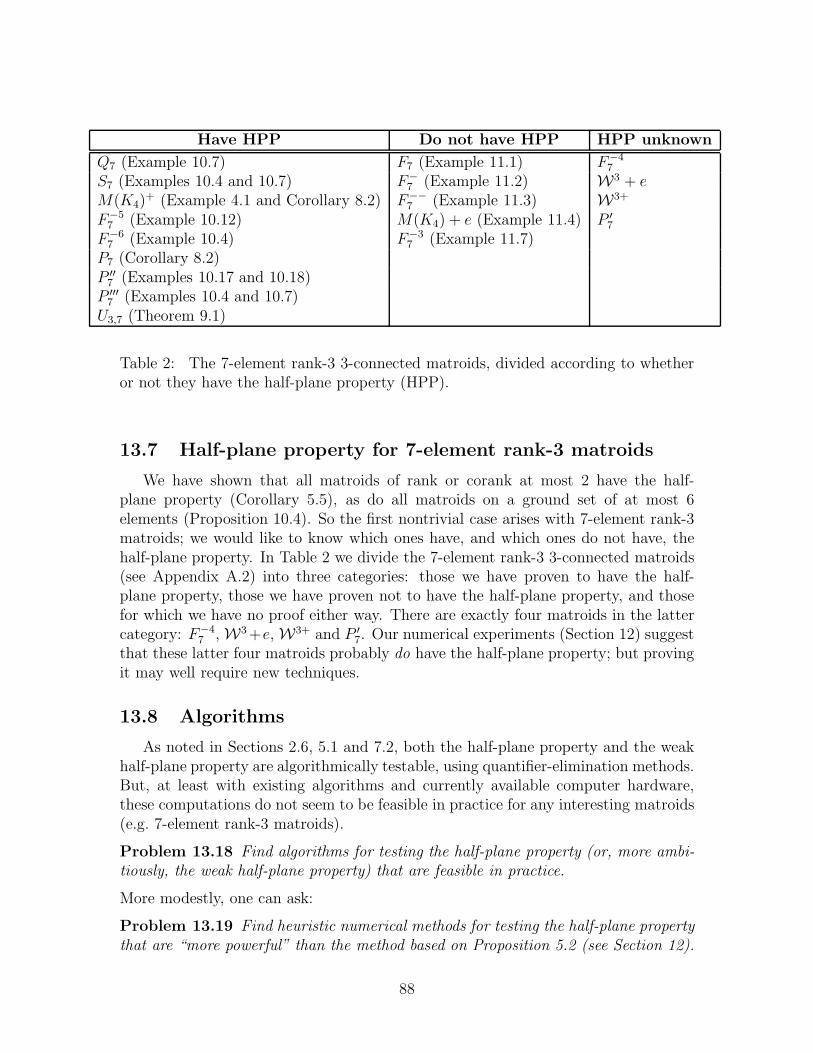
Have HPP Do not have HPP HPP unknown

Q7 (Example 10.7) F7 (Example 11.1) F−47

S7 (Examples 10.4 and 10.7) F−7 (Example 11.2) W3 + e

M(K4)+ (Example 4.1 and Corollary 8.2) F−−

7 (Example 11.3) W3+

F−57 (Example 10.12) M(K4) + e (Example 11.4) P ′

7

F−67 (Example 10.4) F−3

7 (Example 11.7)P7 (Corollary 8.2)P ′′

7 (Examples 10.17 and 10.18)P ′′′

7 (Examples 10.4 and 10.7)U3,7 (Theorem 9.1)

Table 2: The 7-element rank-3 3-connected matroids, divided according to whetheror not they have the half-plane property (HPP).

13.7 Half-plane property for 7-element rank-3 matroids

We have shown that all matroids of rank or corank at most 2 have the half-plane property (Corollary 5.5), as do all matroids on a ground set of at most 6elements (Proposition 10.4). So the first nontrivial case arises with 7-element rank-3matroids; we would like to know which ones have, and which ones do not have, thehalf-plane property. In Table 2 we divide the 7-element rank-3 3-connected matroids(see Appendix A.2) into three categories: those we have proven to have the half-plane property, those we have proven not to have the half-plane property, and thosefor which we have no proof either way. There are exactly four matroids in the lattercategory: F−4

7 , W3 +e, W3+ and P ′7. Our numerical experiments (Section 12) suggest

that these latter four matroids probably do have the half-plane property; but provingit may well require new techniques.

13.8 Algorithms

As noted in Sections 2.6, 5.1 and 7.2, both the half-plane property and the weakhalf-plane property are algorithmically testable, using quantifier-elimination methods.But, at least with existing algorithms and currently available computer hardware,these computations do not seem to be feasible in practice for any interesting matroids(e.g. 7-element rank-3 matroids).

Problem 13.18 Find algorithms for testing the half-plane property (or, more ambi-tiously, the weak half-plane property) that are feasible in practice.

More modestly, one can ask:

Problem 13.19 Find heuristic numerical methods for testing the half-plane propertythat are “more powerful” than the method based on Proposition 5.2 (see Section 12).

88

Acknowledgments

We wish to thank Sankar Basu, Jason Brown, Jim Geelen, Russ Lyons, RichardStanley, Dirk Vertigan and Neil White for helpful comments and suggestions. We alsowish to thank James Renegar and Adam Strzebonski for correspondence concern-ing quantifier-elimination algorithms; Jurgen Bokowski, Andreas Dress and BerndSturmfels for correspondence concerning determinants and Grassmann–Plucker iden-tities; and Sankar Basu, Charles Desoer and Paul Penfield for giving us pointers tothe engineering literature. Finally, we wish to thank Marc Noy and Dominic Welshfor organizing the Workshop on Tutte Polynomials and Related Topics (Barcelona,September 2001), at which this work was first presented.

This research was supported in part by NSA grants MDA904–99–1–0030 andMDA904–01–1–0026 (J.G.O.), NSF grants PHY–9900769 and PHY–0099393 (A.D.S.),and an operating grant from NSERC (D.G.W.).

A Matroids considered in this paper

The half-plane property is preserved by direct sums (Proposition 4.4) and 2-sums(Corollary 4.9); moreover, it is trivially preserved by adjoining loops or parallel el-ements. Therefore, we can restrict attention to simple 3-connected matroids. (Infact, every 3-connected matroid with at least 4 elements is automatically simple [55,Proposition 8.1.6].) Since all rank-1 and rank-2 matroids have the half-plane prop-erty (Corollary 5.5), we can restrict attention to matroids of rank ≥ 3. Finally, sincethe half-plane property is invariant under duality (Proposition 4.2), we can restrictattention to matroids of rank ≤ ⌊n/2⌋, where n is the number of elements.

In this appendix we list all 3-connected rank-3 matroids on 6 or 7 elements, as wellas a few larger matroids that will play a role in this paper. We follow where possiblethe notation of [55, Appendix]; further information on many of these matroids canbe found there.

A.1 Rank-3 matroids on 6 elements

The 3-connected rank-3 matroids on 6 elements are shown in Figure 4.

M(K4): Regular (in fact graphic and cographic). Self-dual. Not transversalor cotransversal. Has half-plane property (Theorem 1.1).

W3: F -representable if and only if |F | ≥ 3. Sixth-root-of-unity but notregular. Self-dual. Transversal but not nice; cotransversal but notco-nice (Example 10.3). Has half-plane property (Corollary 8.2).

Q6: F -representable if and only if |F | ≥ 4. Not sixth-root-of-unity. Self-dual. Nice transversal and co-nice cotransversal (Example 10.7). Hashalf-plane property (Corollary 10.3).

89

t t

ttt t

�������T

TTTTTT""""""bbbbbb t t t

tt t

�������T

TTTTTT

M(K4) W3

t tt

t

tt������

HHHHHH

t t ttt t

tt t

ttt

Q6 P6 U3,6

Figure 4: The 3-connected rank-3 matroids on 6 elements. All of these are obtainedfrom M(K4) by a sequence of relaxations.

P6: F -representable if and only if |F | ≥ 5. Not sixth-root-of-unity. Self-dual. Nice transversal and co-nice cotransversal (Examples 10.4 and10.7). Has half-plane property (Corollary 10.3).

U3,6: F -representable if and only if |F | ≥ 4. Not sixth-root-of-unity. Self-dual. Nice transversal and co-nice cotransversal (Example 10.1). Hashalf-plane property (Theorem 9.1).

A.2 Rank-3 matroids on 7 elements

Besides the uniform matroid U3,7, we classify the 3-connected rank-3 matroids on7 elements as follows [65]:

(a) Those with a 4-point line (Figure 5).

(b) Those with no 4-point line:

(b1) Those that are not ω-regular (Figure 6). All of these are obtained fromthe Fano matroid F7 by a sequence of relaxations.

(b2) Those that are ω-regular (Figure 7). All of these are obtained from P7 bya sequence of relaxations.

90

t t tt t t

t����

HHHHHH

1

23

45

6

7t t t t

tt t1 2 3 4

65 7

Q7 S7

t t

ttt t t

�������T

TTTTTT""""""bbbbbb3

7

5

1

4

2 6

t t t

tt

t t�������T

TTTTTT3

7

5

1

4

26

M(K4)+ W3+

Figure 5: The 3-connected rank-3 matroids on 7 elements with a 4-point line.

A.2.1 Matroids with a 4-point line

Q7: F -representable if and only if |F | ≥ 5. Not sixth-root-of-unity. Nicetransversal (Example 10.7); co-transversal but not co-nice (Exam-ple 10.14). Non-nice principal extension of Q6; non-nice free exten-sion ofQ7\7 (Example 4.4). Has half-plane property (Corollary 10.3).

S7: F -representable if and only if |F | ≥ 7. Not sixth-root-of-unity. Nicetransversal (Example 10.7); co-transversal (we don’t know whetheror not it is co-nice). Non-nice principal extension of P6; non-nice freeextension of S7 \ 7. Has half-plane property (Corollary 10.3).

M(K4)+: F -representable if and only if |F | ≥ 3. Sixth-root-of-unity but not

regular. Not transversal or cotransversal. Nice principal extensionof M(K4) with λ1 = λ2 = λ3 = 1/2 (Example 4.1). This matroidis called O7 in [29]. Has half-plane property (Example 4.1 or Corol-lary 8.2).

W3+: F -representable if and only if |F | ≥ 4. Not sixth-root-of-unity.Transversal but not nice (Example 10.3); co-transversal but not co-nice (Example 10.13). Non-nice principal extension of W3; non-niceprincipal extension of Q7 \ 7. Not known whether it has half-planeproperty.

91

t3 t4

t5

t1t7t2 t6

�������T

TTTTTT""""""bbbbbb&%

'$t3 t

4t5

t1t7t2 t6

�������T

TTTTTT""""""bbbbbb t3 t

4t5

t1t7t2 t6

�������T

TTTTTT""""""bbbbbb

F7 F−7 F−−

7

t3 t4

t5

t1t7t2 t6

�������T

TTTTTT""""""bbbbbb t3 t

4t5

t1t7t2 t6

�������T

TTTTTT t3 t

4t5

t1t7t2 t6

�������T

TTTTTT

M(K4) + e F−37 F−4

7

t3 t4

t5

t1t7t2 t6

�������T

TTTTTT t3 t

4t5

t1t7t2 t6

�������T

TTTTTT t3 t t

t1tt2 t

�������

W3 + e F−57 F−6

7

Figure 6: The 3-connected rank-3 non-uniform matroids on 7 elements that have no4-point line and are not ω-regular. All of these are obtained from the Fano matroidF7 by a sequence of relaxations.

92

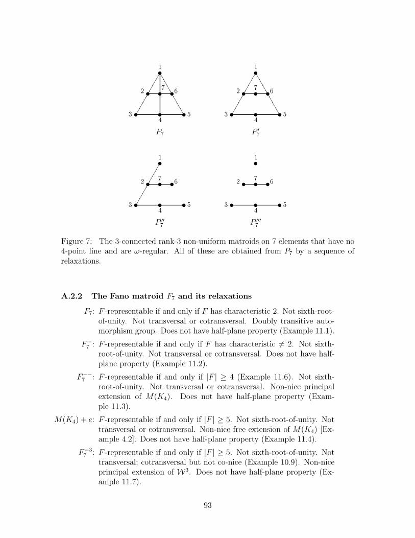
t3 t4

t5

t1t7t2 t6

�������T

TTTTTT t3 t

4t5

t1t7t2 t6

�������T

TTTTTT

P7 P ′7

t3 t4

t5

t1t7t2 t6

�������

t3 t4

t5

t1t7t2 t6

P ′′7 P ′′′

7

Figure 7: The 3-connected rank-3 non-uniform matroids on 7 elements that have no4-point line and are ω-regular. All of these are obtained from P7 by a sequence ofrelaxations.

A.2.2 The Fano matroid F7 and its relaxations

F7: F -representable if and only if F has characteristic 2. Not sixth-root-of-unity. Not transversal or cotransversal. Doubly transitive auto-morphism group. Does not have half-plane property (Example 11.1).

F−7 : F -representable if and only if F has characteristic 6= 2. Not sixth-

root-of-unity. Not transversal or cotransversal. Does not have half-plane property (Example 11.2).

F−−7 : F -representable if and only if |F | ≥ 4 (Example 11.6). Not sixth-

root-of-unity. Not transversal or cotransversal. Non-nice principalextension of M(K4). Does not have half-plane property (Exam-ple 11.3).

M(K4) + e: F -representable if and only if |F | ≥ 5. Not sixth-root-of-unity. Nottransversal or cotransversal. Non-nice free extension of M(K4) [Ex-ample 4.2]. Does not have half-plane property (Example 11.4).

F−37 : F -representable if and only if |F | ≥ 5. Not sixth-root-of-unity. Not

transversal; cotransversal but not co-nice (Example 10.9). Non-niceprincipal extension of W3. Does not have half-plane property (Ex-ample 11.7).

93

F−47 : F -representable if and only if |F | ≥ 4. Not sixth-root-of-unity. Not

transversal; cotransversal but not co-nice (Example 10.10). Non-nice principal extension of Q6. Not known whether it has half-planeproperty.

W3 + e: F -representable if and only if |F | ≥ 5. Not sixth-root-of-unity.Transversal but not nice (Example 10.3); cotransversal but not co-nice (Example 10.11). Non-nice free extension of W3; non-nice prin-cipal extension of Q6. Not known whether it has half-plane property.

F−57 : F -representable if and only if |F | ≥ 5. Not sixth-root-of-unity.

Transversal but not nice (Example 10.8); co-nice cotransversal (Ex-ample 10.12). Non-nice free extension of Q6; non-nice principal ex-tension of P6. Has half-plane property (Corollary 10.3).

F−67 : F -representable if and only if |F | ≥ 7. Not sixth-root-of-unity. Nice

transversal (Example 10.4); co-transversal (we don’t know whetheror not it is co-nice). Non-nice free extension of P6; non-nice principalextension of U3,6. Has half-plane property (Corollary 10.3).

A.2.3 P7 and its relaxations

P7: F -representable if and only if |F | ≥ 3. Sixth-root-of-unity but notregular. k-regular for all k ≥ 1 (see [66]). Not transversal or co-transversal. Has half-plane property (Corollary 8.2).

P ′7: F -representable if and only if |F | ≥ 4. k-regular for all k ≥ 2 (see

[66]). Not transversal; cotransversal but not co-nice (Example 10.16).Non-nice principal extension of W3. Not known whether it has half-plane property.

P ′′7 : F -representable if and only if |F | ≥ 5. k-regular for all k ≥ 3 (see

[66]). Transversal but not nice (Example 10.15); co-nice cotransver-sal (Examples 10.17 and 10.18). Non-nice principal extension of Q6;non-nice principal extension of R6. Has half-plane property (Corol-lary 10.3).

P ′′′7 : F -representable if and only if |F | ≥ 7. k-regular for all k ≥ 4 (see

[66]). Nice transversal (Examples 10.4 and 10.7); co-transversal (wedon’t know whether or not it is co-nice). Non-nice free extensionof R6; non-nice principal extension of P6. Has half-plane property(Corollary 10.3).

A.3 Some rank-3 matroids on 8 or 9 elements

The matroids F−47 , W3 + e, W3+ and P ′

7 play a special role in this paper, as theyare the only rank-3 7-element matroids for which we are unable to prove whether or

94

t3 t4

t5

t1t7t2 t6 t8

�������T

TTTTTT t3 t

4t5

t1t7t8

t2 t6�������T

TTTTTT

F−47 + e W3 + e+ f

t t t

tt

t t�������T

TTTTTT3

7

5

1

4

26t8

t3 t4

t5

t1t7t2 t6

�������T

TTTTTT

t8

W3+ + e P ′7 + e

Figure 8: Some rank-3 8-element matroids that are free extensions of rank-3 7-element matroids.

not they have the half-plane property. Since our numerical experiments (Section 12)suggest that they probably do have the half-plane property, we have also investigatedsome single-element extensions of these matroids in an (unsuccessful) effort to find onethat fails the half-plane property. For brevity we discuss here only the four matroidsthat are obtained as free extensions (see Figure 8):

F−47 + e: F -representable if and only if |F | ≥ 7. Not sixth-root-of-unity. Not

transversal; cotransversal but not co-nice (Example 10.10). Niceprincipal extension of F−4

7 with λ1 = 0, λ2 = . . . = λ7 = 1/4 (Exam-ple 4.3). Every single-element deletion is isomorphic to F−4

7 , F−57 or

U3,7. Not known whether it has half-plane property.

W3 + e+ f : F -representable if and only if |F | ≥ 7. Not sixth-root-of-unity.Transversal but not nice (Example 10.3); cotransversal but not co-nice (Example 10.11). Non-nice free extension of W3 + e. Everysingle-element deletion is isomorphic to W3 + e, F−5

7 or F−67 . Not

known whether it has half-plane property.

W3+ + e: F -representable if and only if |F | ≥ 7. Not sixth-root-of-unity.Transversal but not nice (Example 10.3); cotransversal but not co-nice (Example 10.13). Non-nice free extension of W3+. Every single-element deletion is isomorphic to Q7, S7, W3+, W3 + e or F−5

7 . Notknown whether it has half-plane property.

95

s s s

s s ss s s

��

��

��

��

��

��

��

��

��

��

��

��

��

��Q

QQ

QQ

QQ

QQ

QQ

Q

SS

SS

SS

SS

SS

SS

SS

SS

4 5 6

1 2 3

78

9

s s s

s s ss s s

��

��

��

��

��

��

��

��

��

��

��

��

��

��Q

QQ

QQ

QQ

QQ

QQ

Q

SS

SS

SS

SS

SS

SS

SS

SS

4 5 6

1 2 3

78

9

Pappus non-Pappus

s s s

s s ss s s

��

��

��

��

��

��

��

��

��

��Q

QQ

QQ

QQ

QQ

QQ

Q

SS

SS

SS

SS

4 5 6

1 2 3

78

9

(non-Pappus \ 9) + e

Figure 9: The Pappus and non-Pappus matroids, along with the free extension(non-Pappus \ 9) + e.

P ′7 + e: F -representable if and only if |F | ≥ 7. Not sixth-root-of-unity. Not

transversal; cotransversal but not co-nice (Example 10.16). Non-nice free extension of P ′

7. Every single-element deletion is isomorphicto W3 + e, F−5

7 , P ′7 or P ′′′

7 . Not known whether it has half-planeproperty.

The Pappus and non-Pappus matroids have rank 3 and 9 elements, and are shownin Figure 9. We also consider some related matroids: the deletions non-Pappus\1 andnon-Pappus\9, and the free extension (non-Pappus \ 9)+ e. These matroids have thefollowing properties:

Pappus: F -representable if and only if |F | = 4 or |F | ≥ 7.22 Not sixth-root-of-unity. Not transversal or cotransversal. Transitive automorphismgroup. Every single-element deletion is isomorphic to non-Pappus\9.Does not have half-plane property (Example 11.9).

non-Pappus: Not representable over any field. Not sixth-root-of-unity. Not transver-sal or cotransversal. Every single-element deletion is isomorphic to

22 The assertion on [55, p. 516] is in error.

96

non-Pappus\1 or non-Pappus\9. Does not have half-plane property(Example 11.9).

non-Pappus\1: F -representable if and only if |F | ≥ 5. Not sixth-root-of-unity. Nottransversal; cotransversal but not co-nice (Example 10.19). Everysingle-element deletion is isomorphic to F−4

7 , W3 + e, F−57 , P ′

7 or P ′′7 .

Not known whether it has half-plane property.

non-Pappus\9: F -representable if and only if |F | ≥ 4. Not sixth-root-of-unity. Nottransversal or cotransversal. Every single-element deletion is isomor-phic to F−4

7 or P ′7. Not known whether it has half-plane property.

(non-Pappus \ 9) + e: F -representable if |F | ≥ 7. Not sixth-root-of-unity. Not transver-sal or cotransversal. Every single-element deletion is isomorphic toF−4

7 + e, P ′7 + e or non-Pappus\9. Does not have half-plane property

(Example 11.10).

A.4 Some rank-4 matroids on 8 elements

The rank-4 matroid P8 is represented over any field of characteristic 6= 2 by thematrix23

1 0 0 0 0 1 1 20 1 0 0 1 0 1 10 0 1 0 1 1 0 10 0 0 1 2 1 1 0

(A.1)

A geometric representation of P8 over the reals can be obtained by starting from a 3-dimensional cube and then rotating one face of the cube by 45◦ in its plane [29, Figure14]. There is a unique pair of disjoint circuit-hyperplanes in P8, namely {1, 4, 5, 8}and {2, 3, 6, 7}. We denote by P ′

8 (resp. P ′′8 ) the matroid obtained from P8 by relaxing

one (resp. both) of these circuit-hyperplanes.The Vamos matroid V8 also has rank 4; it is pictured in [55, p. 76, Figure 2.4].

P8: F -representable if and only if F has characteristic 6= 2. Not sixth-root-of-unity. Self-dual. Not transversal or cotransversal. Transitiveautomorphism group. Every single-element contraction is isomor-phic to P7; every single-element deletion is isomorphic to (P7)

∗. See[29, 30] for more information. Does not have half-plane property(Example 11.8).

P ′8: F -representable if and only if |F | ≥ 4. Not sixth-root-of-unity. Self-

dual. Not transversal or cotransversal. Every single-element con-traction is isomorphic to P7 or P ′

7; every single-element deletion isisomorphic to (P7)

∗ or (P ′7)

∗. Does not have half-plane property (Ex-ample 11.8).

23 The GF (3)-representation of P8 on [55, p. 512] has a misprint: the bottom right element shouldbe 0, not 1.

97

P ′′8 : F -representable if and only if |F | ≥ 5. Not sixth-root-of-unity. Self-

dual. Not transversal or cotransversal. Transitive automorphismgroup. Every single-element contraction is isomorphic to P ′

7; everysingle-element deletion is isomorphic to (P ′

7)∗. See [29, 30] for more

information. Does not have half-plane property (Example 11.8).

V8: Not representable over any field. Not sixth-root-of-unity. Self-dual.Not transversal or cotransversal. Every single-element contraction isisomorphic to F−4

7 or F−57 ; every single-element deletion is isomorphic

to (F−47 )∗ or (F−5

7 )∗. Not known whether it has half-plane property.

A.5 Some transversal matroids

Some interesting transversal matroids are introduced in Sections 10.3 and 10.4.In particular, all rank-3 transversal matroids are classified in Section 10.4; and therank-(n+ 1) transversal matroid Nn is defined in Example 10.18.

B (F, {1})-representability of matroids

We defined (F,G)-representations of matroids in Section 8.2 and noted that, when−1 ∈ G, such representations are covered under the theory of partial fields developedby Semple and Whittle [67]. When −1 /∈ G, the class of (F,G)-representable matroidsis less well-behaved. For example, neither reordering the columns, reordering therows, nor pivoting is guaranteed to produce another (F,G)-representation. In thisappendix, we consider (F,G)-representable matroids in the case that G is the trivialgroup {1}, and we characterize such matroids. If F has characteristic 2, then it isclear that a matroid M is (F, {1})-representable if and only if M is binary. When thecharacteristic of F is not 2, the determination of all (F, {1})-representable matroids,which is contained in Theorem B.1, is more difficult.

We now inductively define when a graph is a chain of cycles .

(i) A single cycle C of length at least three is a chain of cycles, which we write as(C).

(ii) Suppose that (C1, C2, . . . , Cn) is a chain of cycles and that each of C1, C2, . . . , Cn

is a cycle. Let e be an edge of Cn that is in none of C1, C2, . . . , Cn−1 andlet Cn+1 be a cycle of length at least three that contains e but no otheredge of (C1, C2, . . . , Cn). Let (C1, C2, . . . , Cn+1) be the parallel connection of(C1, C2, . . . , Cn) and Cn+1 across the edge e. Then (C1, C2, . . . , Cn+1) is a chainof cycles.

A graph G′ is an augmented chain of cycles if G′ can be obtained from a chain ofcycles G by adding some (possibly empty) set of edges so that each added edge isparallel to some edge of G.

98

The next theorem is the main result of this appendix. The graph G6 has 6 verticesand 9 edges and is obtained by attaching a triangle via parallel connection to eachedge of a triangle.

Theorem B.1 The following statements are equivalent for a matroid M and a fieldF of characteristic other than 2.

(i) M is (F, {1})-representable.

(ii) Each component of M is a loop, a rank-1 uniform matroid, or the cycle matroidof an augmented chain of cycles.

(iii) M has no minor isomorphic to U2,4,M(K4),M(K2,3), or M(G6).

A consequence of Theorem B.1 is that, when the characteristic of F is not 2, theclass of (F, {1})-representable matroids is not closed under duality. For example, if Gis the graph that is obtained from G6 by contracting one edge incident with a degree-2vertex, then G is an augmented chain of cycles, so M(G) is (F, {1})-representable.However, M∗(G) has M(K2,3) as a minor and so is not (F, {1})-representable. Wecan also use M(G) to show that, when the characteristic of F is not 2, the classof (F, {1})-representable matroids is not closed under 2-sum, series connection, orparallel connection. To see this, we observe that M(G6) is the 2-sum of M(G) andthe graph obtained by adding an edge parallel to one edge of a triangle; M(G6) is alsothe series connection of M(G) and U1,2; and, finally, M(G6) is the parallel connectionof the simplification of M(G) and a triangle.

The proof of Theorem B.1 will use the following definition. Fix an integer r ≥ 1;and, for 1 ≤ i ≤ r, let ei be the column vector of length r with a 1 in the ith row andzeros elsewhere. An r × n matrix A will be called special if:

(a) the first column is e1, and the last column is er;

(b) each column is either ei or ei + ei+1;

(c) a column ei is always followed by either ei or ei + ei+1; and

(d) a column ei + ei+1 is always followed by either ei + ei+1, ei+1, or ei+1 + ei+2.

Note that a special matrix may have repeated columns; but if two columns are equalto c, say, then all intermediate columns must also be equal to c.

The next result is the main step in the proof of Theorem B.1.

Proposition B.2 Let A be an (F, {1})-representation of a connected loopless matroidM . If the number of rows of A equals r(M), then A is special.

99

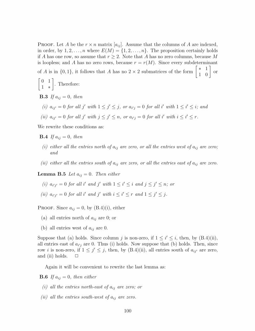
Proof. Let A be the r× n matrix [aij ]. Assume that the columns of A are indexed,in order, by 1, 2, . . . , n where E(M) = {1, 2, . . . , n}. The proposition certainly holdsif A has one row, so assume that r ≥ 2. Note that A has no zero columns, because Mis loopless; and A has no zero rows, because r = r(M). Since every subdeterminant

of A is in {0, 1}, it follows that A has no 2 × 2 submatrices of the form

[∗ 11 0

]or

[0 11 ∗

]. Therefore:

B.3 If aij = 0, then

(i) aij′ = 0 for all j′ with 1 ≤ j′ ≤ j, or ai′j = 0 for all i′ with 1 ≤ i′ ≤ i; and

(ii) aij′ = 0 for all j′ with j ≤ j′ ≤ n, or ai′j = 0 for all i′ with i ≤ i′ ≤ r.

We rewrite these conditions as:

B.4 If aij = 0, then

(i) either all the entries north of aij are zero, or all the entries west of aij are zero;and

(ii) either all the entries south of aij are zero, or all the entries east of aij are zero.

Lemma B.5 Let aij = 0. Then either

(i) ai′j′ = 0 for all i′ and j′ with 1 ≤ i′ ≤ i and j ≤ j′ ≤ n; or

(ii) ai′j′ = 0 for all i′ and j′ with i ≤ i′ ≤ r and 1 ≤ j′ ≤ j.

Proof. Since aij = 0, by (B.4)(i), either

(a) all entries north of aij are 0; or

(b) all entries west of aij are 0.

Suppose that (a) holds. Since column j is non-zero, if 1 ≤ i′ ≤ i, then, by (B.4)(ii),all entries east of ai′j are 0. Thus (i) holds. Now suppose that (b) holds. Then, sincerow i is non-zero, if 1 ≤ j′ ≤ j, then, by (B.4)(ii), all entries south of aij′ are zero,and (ii) holds. 2

Again it will be convenient to rewrite the last lemma as:

B.6 If aij = 0, then either

(i) all the entries north-east of aij are zero; or

(ii) all the entries south-west of aij are zero.

100

By combining (B.3) with the fact that A has no zero rows and no zero columns,we deduce that no column of A has [1 0 1]T as a submatrix and no row of A has [1 0 1]as a submatrix. Thus every column of A and every row of A consists of a (possiblyempty) sequence of zeros, followed by a non-empty sequence of ones, followed by a(possibly empty) sequence of zeros.

Let D3 be the matrix

1 1 01 1 10 1 1

. Then D3 has determinant −1 and so the next

lemma is immediate.

Lemma B.7 The matrix A does not have D3 as a submatrix.

Lemma B.8 If aij = 1 and a(i+1)j = 0, then j < n and ai(j+1) = 1.

Proof. If j = n, then, since aij = 1, it follows by (B.4) that row i+ 1 of A is zero;a contradiction. Thus j < n. Suppose that ai(j+1) = 0. Then, by (B.6), all entriesnorth-east of ai(j+1) are zero and all entries south-west of a(i+1)j are zero. Thus A has

the block form

[A1 00 A2

]and so M is disconnected; a contradiction. 2

By a similar argument to that just given, we get:

Lemma B.9 If aij = 0 and a(i+1)j = 1, then j ≥ 2 and a(i+1)(j−1) = 1.

Lemma B.10 ar1 = 0 = a1n.

Proof. Suppose that ar1 = 1. If ai1 = 0 for some i < r, then, by (B.5), row i is zero;a contradiction. Thus column 1 of A consists of all ones and, similarly, row r consistsof all ones. Since r ≥ 2, there is a column of A that does not consist of all ones. Letj be the first such column. Then aj1 = 0 and {1, 2, . . . , j − 1} is the ground set ofa rank-1 component of M ; a contradiction. We conclude that ar1 = 0, and a similarargument shows that a1n = 0. 2

Assume now that Proposition B.2 is false, and let A be a counterexample havingthe minimum number of columns. In particular, no two consecutive columns of A areequal. The following lemmas derive some properties of this minimal counterexample,culminating in a contradiction.

Lemma B.11 Every column of A has at most two ones.

Proof. Suppose that, for some j with 1 < j < n, column j has a unique one,which occurs in row i say. Then 1 < i < r, and every entry north-east of a(i−1)j iszero, as is every entry south-west of a(i+1)j . Thus M/j is disconnected, so M is aparallel connection with basepoint j. Indeed, M is the parallel connection of M [A1]

101

and M [A2] where A1 is the submatrix of A that consists of aij and all entries to itsnorth-west, and A2 is the submatrix of A that consists of aij and all entries to itssouth-east. Since M is connected, so are both M [A1] and M [A2]. It follows that bothA1 and A2 are special matrices and, therefore, so is A; a contradiction. Thus everycolumn of A except possibly the first or the last has at least two ones.

Now suppose that A has a single one in its first column. Then a11 = 1. Supposethat M/1 is connected. Let A1 be the matrix obtained from A by deleting the firstrow and column. Then A1 is special. By Lemma B.10, a1n = 0. Let the first zeroentry in row 1 of A be a1m. Then m ≥ 3 otherwise 1 is a coloop of M . Nowa11 = a12 = . . . = a1(m−1) = 1. Moreover, a22 = a23 = . . . = a2(m−1) = 1 otherwiseM [A1] has a loop. Since A has no consecutive equal columns and A1 is special, m ≤ 4.If m = 3, then columns 1 and 2 of A are [1 0 0 . . . 0]T and [1 1 0 . . . 0]T, and it followsthat A is special; a contradiction. We may now suppose that m = 4. Then a24 = 0otherwise the submatrix of A determined by the first three rows and columns 2, 3,and 4 is D3; a contradiction. Thus a2j = 0 for all j ≥ 4. Now the matrix A representsM over F . If we subtract row 2 from row 1 in A, we get another F -representationfor M , which shows that 1 is a coloop of M ; a contradiction.

We may now assume that M/1 is disconnected. Then M\1 is connected. Itfollows that the matrix A\1, which is obtained from A by deleting the first column,is special. Thus column 2 of A equals e1. Therefore column 1 is parallel to column 2;a contradiction.

We conclude that the first column of A has at least two ones, and, by symmetry,the last column of A has at least two ones. 2

A submatrix C of a matrix D will be called consecutive if the rows of C areconsecutive rows of D and the columns of C are consecutive columns of D.

Lemma B.12 A has

[1 10 1

]as a consecutive submatrix.

Proof. Proceed north from ar1, which we know from Lemma B.10 is 0, until the

first 1 is reached. Then we have

[10

]as a submatrix meeting consecutive rows. Then

proceed east from the 0 in this submatrix until the first 1 is met. By Lemma B.8,

we deduce that A has

[1 1 . . . 1 10 0 . . . 0 1

]as a consecutive submatrix, and the lemma

follows. 2

Let J ′k be the k × k matrix all of whose entries are one except for that in the

south-west corner, which is zero.

Lemma B.13 Every consecutive J ′2-submatrix of A is contained in a consecutive J ′

3-submatrix of A.

102

Proof. Suppose that

c11 c12 c131 1 c230 1 c33

is a consecutive submatrix C of A containing

[1 10 1

]as a submatrix. The additional row must exist and c11 = 1 otherwise A has

a column with a single one. The additional column must exist and c33 = 1 otherwiseA has a row with a single one and so has a coloop.

Suppose c12 = 0. Then adjoin an additional column x to A that is zero everywhereexcept in the row corresponding to the second row of C. This column should beadded between the first and second columns of C with the resulting matrix beingA′. The matroid M [A′]/x is disconnected. Thus M [A] is the 2-sum of two matroidswith basepoint x. Let A′

1 be the submatrix of A′ consisting of the non-zero entry incolumn x and all entries north-west of it, and A′

2 be the submatrix of A′ consistingof the non-zero entry in column x and all entries south-east of it. Then M [A′] isthe parallel connection of M [A′

1] and M [A′2] and so each of these is connected. Since

A has a submatrix equal to A′1, the last matrix is an (F, {1})-representation for a

connected matroid. Since A′2 is obtained by adjoining the column [1 0 0 . . . 0]T to

the beginning of a submatrix of A, it too is an (F, {1})-representation for a connectedmatroid. Thus each of A′

1 and A′2 is special. It follows that A′ is special and so too

is A; a contradiction. We conclude that c12 = 1.Suppose c23 = 0. Let y be the column of A corresponding to the second column of

C. Then A\y has the form

[A1 00 A2

]and so M\y is disconnected and the rank of A

is the sum of the ranks, r1 and r2, say, of A1 and A2. We may apply row operationsin A to transform A2 into a matrix that has a permutation of Ir2 as a submatrix.These row operations will not affect the first r1 rows of A. Then, by contracting theelements of M corresponding to the columns of Ir2 , we see that the submatrix A′′

1

consisting of A1 and the first r1 rows of column y represents a connected matroid.This is because M is the series connection of this matroid and another with respectto the basepoint y. Thus A′′

1 is special. But the last column of A′′1 has more than one

one; a contradiction. We conclude that c23 = 1.Finally, since D3 is not a submatrix of A, we deduce that c13 = 1. 2

Lemma B.14 For all k ≥ 2, the matrix A has J ′k as a consecutive submatrix.

Proof. We shall argue by induction. By the last two lemmas, A has J ′2 and J ′

3 asconsecutive submatrices. Assume that A has J ′

m as a consecutive submatrix, for somem ≥ 3. The rows i and i+ 1 of A that correspond to rows 1 and 2 of J ′

m must differ.Therefore, in A, the submatrix induced by rows i and i+ 1 has either

(i) in the consecutive columns immediately after J ′m, a 2× t matrix H1 of the form[

1 1 . . . 1 01 1 . . . 1 1

]for some t ≥ 1;

103

(ii) in the consecutive columns immediately before J ′m, a 2 × s matrix H2 of the

form

[1 1 . . . 1 10 1 . . . 1 1

]for some s ≥ 1.

In case (i), the column of A corresponding to the last column ofH1 must have onesin the m−1 rows immediately below the unique zero otherwise (B.6) is contradicted.It follows that A has D3 as a submatrix; a contradiction.

In case (ii), the unique zero in H2 is in a consecutive submatrix of A equal toJ ′

2. Thus, by Lemma B.13, the (i− 1)st row of A must have ones in all the columnscorresponding to those of J ′

m otherwise A has D3 as a submatrix. We deduce that Ahas, as a consecutive submatrix, the matrix J ′′

m that is obtained by adjoining a rowof ones to the beginning of J ′

m.The columns j and j+1 of A that correspond to the last two columns of J ′′

m mustdiffer. If they differ in some row before row i−1 of A, let row u be the highest indexedsuch row where they differ. This row has [1 0] in columns j and j+ 1 of A. Then, byLemma B.5, auj = au(j−1) = . . . = au(j−m+2) = 1 and so A has D3 as a submatrix; acontradiction. We deduce that columns j and j + 1 of A differ in some row after rowi + m − 1. Let row v be the smallest indexed such row where these columns differ.Then [

a(v−1)j a(v−1)(j+1)

avj av(j+1)

]= J ′

2 .

By Lemma B.13, this J ′2 is contained in a consecutive submatrix of A equal to J ′

3.To avoid having D3 as a submatrix of A, it follows that a(i−1)(j+2) = ai(j+2) = . . . =a(i+m−1)(j+2) = 1. Thus A has J ′

m+1 as a consecutive submatrix and the lemma followsby induction. 2

Proposition B.2 follows immediately from the last lemma since it implies that thematrix A is infinite. 2

Lemma B.15 If A is a special matrix, then every square submatrix of A has deter-minant in {0, 1}.

Proof. We argue by induction on the number n of columns of A. If n = 1, then theresult is immediate. Assume the result holds for n = k and let n = k + 1. Now letA′ be a square submatrix of A. We may assume that the columns of A are distinctsince if A′ has repeated columns, its determinant is 0. If A′ meets the first column ofA, then detA′ = 0 unless A′ meets the first row of A. In the exceptional case, detA′

equals the determinant of the submatrix A′1 of A′ that is obtained by deleting the

first row and column. Now A′1 is a submatrix of A1, the matrix obtained by deleting

the first row and column of A. Moreover, it is not difficult to see that A1 is special.Thus, by induction, detA′ ∈ {0, 1}. We may now assume that A′ does not meet thefirst column of A. If A′ does not meet the first row of A, then A′ is a submatrix of

104

the special matrix A1 and the result follows by the induction assumption. Thus wemay assume that A′ contains the entry a12 of A otherwise detA′ = 0. Since a12 isthe only non-zero entry of the first row of A′, we have detA′ = detA′

1. But A′1 is

a submatrix of the special matrix A1 and again the result follows by the inductionassumption. 2

We are now ready to prove Theorem B.1.

Proof of Theorem B.1. We shall show first that (ii) implies (iii). Suppose thatM satisfies (ii). Then every minor of M also satisfies (ii). The construction of Mguarantees that M is the cycle matroid of a series-parallel network G. Thus M has nominor isomorphic to U2,4 or M(K4). Moreover, G is an outerplanar graph, so M hasno minor isomorphic to M(K2,3). Finally, we observe that M does not have M(G6)as a minor since G6 cannot be written as a chain of cycles. Thus (iii) holds.

Next we show that (iii) implies (ii). Suppose thatM is a simple connected matroidthat satisfies (iii) and has rank at least two, and assume that M is a minor-minimalmatroid that does not satisfy (ii). The fact that M has none of U2,4,M(K4), andM(K2,3) as a minor ensures that M ∼= M(G) where G is an outerplanar graph withat least three vertices. Take an outerplanar embedding of G. The boundary of theinfinite face is a Hamilton cycle C of G and all edges not in C are chords of C.Certainly no chords of C cross. Now take a chord e of C with endpoints x and y, say,such that there is an xy-path P1 in C such that every vertex of V (P1) − {x, y} hasdegree 2 in G. Then M\P1 satisfies (iii) and hence also satisfies (ii). Thus M\P1 isthe cycle matroid of a chain of cycles (C1, C2, . . . , Cn), and M is obtained by takingthe parallel connection of M\P1 and the circuit with ground set P1 ∪ e. If e is anedge of C1 that is in no other Ci, then M is the cycle matroid of a chain of cycles.Therefore, by symmetry, we may now assume that either e is an edge that is commonto Ci and Ci+1 for some i, or e is in exactly one Cj for some j in {2, 3, . . . , n − 1}.The first case cannot arise because G is outerplanar. The second case implies withoutdifficulty that M(G) has a minor isomorphic to M(G6). This contradiction impliesthat M satisfies (ii).

Now suppose that M satisfies (ii). We shall show that M satisfies (i). If the com-ponents M1,M2, . . . ,Mm of M have (F, {1})-representations A1, A2, . . . , Am, respec-tively, then the matrix whose block form has A1, A2, . . . , Am on the main diagonal andzeros elsewhere is an (F, {1})-representation forM . Thus it suffices to prove that eachcomponent of M satisfies (i). Clearly a loop and a coloop are (F, {1})-representable.Moreover, if the simple matroid associated with M is (F, {1})-representable, then sotoo is M . Thus we may assume that M is simple. Let C be a k-cycle for some k ≥ 3.Then the (k − 1) × k matrix with columns e1, e1 + e2, e2 + e3, . . . , ek−2 + ek−1, ek−1

is an F -representation for M [C]. The construction of a representation for a paral-lel connection of two matroids is straightforward (see, for example, [55, Proposition7.1.21]). Using this, it is not difficult to show that the cycle matroid of a chain ofcycles can be represented by a special matrix. It follows by Lemma B.15 that M

105

satisfies (i).Finally, we show that (i) implies (ii). Assume that M is (F, {1})-representable

and consider a component M ′ of M of rank at least two. Let A be an (F, {1})-representation for M ′. We may assume that A has r(M ′) rows otherwise we candelete some row from A and still retain an (F, {1})-representation for M ′. Then, byProposition B.2, A is special. From the definition of a special matrix, it is not difficultto see that M ′ is the cycle matroid of an augmented chain of cycles. 2

References

[1] L.V. Ahlfors, Complex Analysis (McGraw-Hill, New York, 1966).

[2] N. Anderson, E.B. Saff and R.S. Varga, On the Enestrom–Kakeya theorem andits sharpness, Lin. Alg. Appl. 28 (1979), 5–16.

[3] T. Asano, Theorems on the partition functions of the Heisenberg ferromagnets,J. Phys. Soc. Japan 29 (1970), 350–359.

[4] R.B. Bapat and T.E.S. Raghavan, Nonnegative Matrices and Applications (Cam-bridge University Press, Cambridge–New York, 1997).

[5] S. Basu, R. Pollack and M.-F. Roy, On the combinatorial and algebraic com-plexity of quantifier elimination, J. ACM 43 (1996), 1002–1045.

[6] J. Bokowski and B. Sturmfels, Computational Synthetic Geometry , Lecture Notesin Mathematics #1355 (Springer-Verlag, Berlin–Heidelberg, 1989).

[7] N.K. Bose, A note on multivariable positive real functions, IEEE Trans. CircuitTheory CT–19 (1972), 194–195.

[8] A. Bouchet and W.H. Cunningham, Delta-matroids, jump systems, and bisub-modular polyhedra, SIAM J. Discrete Math. 8 (1995), 17–32.

[9] R.L. Brooks, C.A.B. Smith, A.H. Stone and W.T. Tutte, The dissection of rect-angles into squares, Duke Math. J. 7 (1940), 312–340.

[10] J.I. Brown and C.J. Colbourn, Roots of the reliability polynomial, SIAM J.Discrete Math. 5 (1992), 571–585.

[11] R.A. Brualdi, Transversal matroids, in Combinatorial Geometries, edited byNeil White, Encyclopedia of Mathematics and its Applications #29 (CambridgeUniversity Press, Cambridge, 1987), Chapter 5, pp. 72–97.

[12] O. Brune, Synthesis of a finite two-terminal network whose driving-pointimpedance is a prescribed function of frequency, J. Math. and Phys. 10 (1931),191–236.

106

[13] T.H. Brylawski, An affine representation for transversal geometries, Stud. Appl.Math. 54 (1975), 143–160.

[14] T. Brylawski, Constructions, in Theory of Matroids, edited by Neil White, Ency-clopedia of Mathematics and its Applications #26 (Cambridge University Press,Cambridge, 1986), Chapter 7, pp. 127–223.

[15] B.F. Caviness and J.R. Johnson, editors, Quantifier Elimination and CylindricalAlgebraic Decomposition (Springer-Verlag, Wien–New York, 1998).

[16] S. Chaiken, A combinatorial proof of the all minors matrix-tree theorem, SIAMJ. Alg. Disc. Meth. 3 (1982), 319–329.

[17] S. Chaiken and D.J. Kleitman, Matrix tree theorems, J. Combin. Theory A 24(1978), 377–381.

[18] W.-K. Chen, Applied Graph Theory (North-Holland, Amsterdam–London, 1971).

[19] C.J. Colbourn, The Combinatorics of Network Reliability (Oxford UniversityPress, New York–Oxford, 1987).

[20] G.E. Collins, Quantifier elimination for real closed fields by cylindrical alge-braic decomposition, in Automata Theory and Formal Languages (Lecture Notesin Computer Science #33), edited by H. Brakhage (Springer-Verlag, Berlin–Heidelberg–New York–Tokyo, 1975), pp. 134–183. Reprinted in: Quantifier Elim-ination and Cylindrical Algebraic Decomposition, edited by B.F. Caviness andJ.R. Johnson (Springer-Verlag, Wien–New York, 1998), pp. 85–121.

[21] W.H. Cunningham, A combinatorial decomposition theory, Ph.D. thesis, Uni-versity of Waterloo, 1973.

[22] D.M. Cvetkovic, M. Doob and H. Sachs, Spectra of Graphs: Theory and Appli-cations (Academic Press, New York–San Francisco–London, 1980).

[23] C.A. Desoer and E.S. Kuh, Basic Circuit Theory (McGraw-Hill, New York,1969).

[24] R.J. Duffin and T.D. Morley, Wang algebra and matroids, IEEE Trans. Circuitsand Systems 25 (1978), 755–762.

[25] A. Fettweis, Elementary symmetric functions and positive functions in severalvariables, in Signal Processing, Scattering and Operator Theory, and Numeri-cal Methods , edited by M.A. Kaashoek, J.H. van Schuppen and A.C.M. Ran(Birkhauser, Boston–Basel–Berlin, 1990), pp. 91–98.

[26] A. Fettweis and S. Basu, New results on stable multidimensional polynomials —Part I: Continuous case, IEEE Trans. Circuits and Systems 34 (1987), 1221–1232.

107

[27] F.R. Gantmacher, The Theory of Matrices, vol. 2 (Chelsea, New York, 1959).

[28] J.F. Geelen, Lectures on jump systems, Center of Parallel Computing, Universityof Cologne, n.d.

[29] J.F. Geelen, A.M.H. Gerards and A. Kapoor, The excluded minors for GF (4)-representable matroids, J. Combin. Theory B 79 (2000), 247–299.

[30] J.F. Geelen, J.G. Oxley, D.L. Vertigan and G.P. Whittle, On the excluded minorsfor quaternary matroids, J. Combin. Theory B 80 (2000), 57–68.

[31] J.H. Grace, The zeros of a polynomial, Proc. Cambridge Philos. Soc. 11 (1902),352–357.

[32] D.H. Greene and D.E. Knuth, Mathematics for the Analysis of Algorithms, 3rd

ed. (Birkhauser, Boston, 1990).

[33] J. Gregor, On quadratic Hurwitz forms I, Aplikace Matematiky 26, 142–153(1981).

[34] D.Yu. Grigor’ev, Complexity of deciding Tarski algebra. J. Symbolic Comput. 5(1988), 65–108.

[35] O.J. Heilmann and E.H. Lieb, Theory of monomer-dimer systems, Commun.Math. Phys. 25 (1972), 190–232.

[36] J. Heintz, M.F. Roy and P. Solerno, Sur la complexite du principe de Tarski-Seidenberg, Bull. Soc. Math. France 118 (1990), 101–126.

[37] A. Hinkkanen, Schur products of certain polynomials, in Lipa’s Legacy: Proceed-ings of the Bers Colloquium, edited by Jozef Dodziuk and Linda Keen (AmericanMathematical Society, Providence, 1997), Contemp. Math. 211, 285–295.

[38] A.J. Hoffman, Eigenvalues and partitionings of the edges of a graph, LinearAlgebra Appl. 5 (1972), 137–146.

[39] T.W. Hungerford, Algebra (Springer-Verlag, New York, 1974, fifth printing1989).

[40] A.W. Ingleton, Transversal matroids and related structures, in Higher Combina-torics, edited by M. Aigner (Reidel, Dordrecht, 1977), pp. 117–131.

[41] T. Koga, Synthesis of finite passive n-ports with prescribed positive real matricesof several variables, IEEE Trans. Circuit Theory CT–15 (1968), 2–23.

[42] S.G. Krantz, Function Theory of Several Complex Variables, 2nd ed. (Wadsworth& Brooks/Cole, Pacific Grove, California, 1992).

108

[43] S. Krogdahl, The dependence graph for bases in matroids, Discrete Math. 19(1977), 47–59.

[44] J.P.S. Kung, Basis-exchange properties, in Theory of Matroids, edited by NeilWhite, Encyclopedia of Mathematics and its Applications #26 (Cambridge Uni-versity Press, Cambridge, 1986), Chapter 4, pp. 62–75.

[45] J.P.S. Kung, Twelve views of matroid theory, in Combinatorial and Computa-tional Mathematics (Pohang, Korea, 15–17 February 2000), edited by SungpyoHong, Jin Ho Kwah, Ki Hang Kim and Fred W. Roush (World Scientific, Singa-pore, 2001), pp. 56–96.

[46] T.D. Lee and C.N. Yang, Statistical theory of equations of state and phasetransitions. II. Lattice gas and Ising model, Phys. Rev. 87 (1952), 410–419.

[47] E.H. Lieb and A.D. Sokal, A general Lee-Yang theorem for one-component andmulticomponent ferromagnets, Commun. Math. Phys. 80 (1981), 153–179.

[48] L. Lovasz and M.D. Plummer, Matching Theory , North-Holland Mathe-matics Studies #121, Annals of Discrete Mathematics #29 (North-Holland,Amsterdam–New York / Akademiai Kiado, Budapest, 1986).

[49] L. Lovasz, The membership problem in jump systems, J. Combin. Theory B 70(1997), 45–66.

[50] M. Marcus and H. Minc, Introduction to Linear Algebra (Macmillan, New York,1965).

[51] M. Marden, Geometry of Polynomials, 2nd ed., (American Mathematical Society,Providence, R.I., 1966).

[52] J.H. Mason, A characterization of transversal independence spaces, in Theoriedes Matroıdes, (Lecture Notes in Mathematics #211), edited by C.P. Bruter(Springer-Verlag, Berlin, 1971), pp. 86–94.

[53] H. Minc, Permanents (Addison-Wesley, Reading MA, 1978).

[54] C.M. Newman, Zeros of the partition function for generalized Ising systems,Comm. Pure Appl. Math. 27 (1974), 143–159.

[55] J.G. Oxley, Matroid Theory (Oxford University Press, New York, 1992).

[56] J. Oxley, C. Semple and D. Vertigan, Generalized ∆−Y exchange and k-regularmatroids, J. Combin. Theory B 79 (2000), 1–65.

[57] H. Ozaki and T. Kasami, Positive real functions of several variables and theirapplications to variable networks, IEEE Trans. Circuit Theory CT–7 (1960),251–260.

109

[58] P. Penfield, R. Spence and S. Duinker, Tellegen’s Theorem and Electrical Net-works (MIT Press, Cambridge, MA, 1970).

[59] M.J. Piff and D.J.A. Welsh, On the vector representation of matroids, J. LondonMath. Soc. (2) 2 (1970), 284–288.

[60] J. Renegar, On the computational complexity and geometry of the first-ordertheory of the reals. I–III, J. Symbolic Comput. 13 (1992), 255–352.

[61] G. Royle and A.D. Sokal, The Brown–Colbourn conjecture on zeros of reliabilitypolynomials is false, in preparation.

[62] W. Rudin, Function Theory in Polydiscs (Benjamin, New York, 1969).

[63] D. Ruelle, Extension of the Lee-Yang circle theorem, Phys. Rev. Lett. 26 (1971),303–304, 870 (erratum).

[64] D. Ruelle, Some remarks on the location of zeroes of the partition function forlattice systems, Commun. Math. Phys. 31 (1973), 265–277.

[65] C. Semple, k-regular matroids, Ph.D. thesis, Victoria University, Wellington,1998.

[66] C. Semple, On maximum-sized k-regular matroids, Graphs Combin. 15 (1999),441–462.

[67] C. Semple and G. Whittle, Partial fields and matroid representation, Adv. Appl.Math. 17 (1996), 184–208.

[68] B. Simon, The P (ϕ)2 Euclidean (Quantum) Field Theory (Princeton UniversityPress, Princeton, 1974), Section IX.3.

[69] J.H. Smith, Some properties of the spectrum of a graph, in Combinatorial Struc-tures and their Applications (Proceedings of the Calgary International Confer-ence, Calgary, Alberta, 1969), pp. 403–406 (Gordon and Breach, New York,1970).

[70] A.D. Sokal, Bounds on the complex zeros of (di)chromatic polynomials and Potts-model partition functions, Combin. Probab. Comput. 10 (2001), 41–77, cond-mat/9904146 at xxx.lanl.gov.

[71] G. Szego, Bemerkungen zu einem Satz von J. H. Grace uber die Wurzeln al-gebraischer Gleichungen, Math. Z. 13 (1922), 28–55. Reprinted in: G. Szego,Collected Papers , vol. 1, edited by Richard Askey (Birkhauser, Boston–Basel–Stuttgart, 1982), pp. 506–534.

110

[72] A. Tarski, A Decision Method for Elementary Algebra and Geometry (Univer-sity of California Press, Berkeley–Los Angeles, 1951). Reprinted in: QuantifierElimination and Cylindrical Algebraic Decomposition, edited by B.F. Cavinessand J.R. Johnson (Springer-Verlag, Wien–New York, 1998), pp. 24–84.

[73] D.G. Wagner, Zeros of reliability polynomials and f -vectors of matroids. Combin.Probab. Comput. 9 (2000), 167–190.

[74] J.L. Walsh, On the location of the roots of certain types of polynomials, Trans.Amer. Math. Soc. 24 (1922), 163–180.

[75] N. White, Coordinatizations, in Combinatorial Geometries, edited by NeilWhite, Encyclopedia of Mathematics and its Applications #29 (Cambridge Uni-versity Press, Cambridge, 1987), Chapter 1, pp. 1–27.

[76] N. White, Unimodular matroids, in Combinatorial Geometries, edited by NeilWhite, Encyclopedia of Mathematics and its Applications #29 (Cambridge Uni-versity Press, Cambridge, 1987), Chapter 3, pp. 40–52.

[77] G. Whittle, A characterisation of the matroids representable over GF (3) and therationals, J. Combin. Theory B 65 (1995), 222–261.

[78] G. Whittle, On matroids representable over GF (3) and other fields, Trans. Amer.Math. Soc. 349 (1997), 579–603.

[79] H.S. Wilf, Generatingfunctionology , 2nd ed. (Academic Press, Boston, 1994).

[80] D. Zeilberger, A combinatorial approach to matrix algebra, Discrete Math. 56(1985), 61–72.

111