homework 7 - inst.eecs.berkeley.eduee16b/sp18/hw/hw7/sol7.pdf · eecs 16b designing information...

EECS 16B Designing Information Devices and Systems IISpring 2018 J. Roychowdhury and M. Maharbiz Homework 7

This homework is due on Thursday, March 22, 2018, at 11:59AM (NOON).Self-grades are due on Monday, March 26, 2018, at 11:59AM (NOON).

Pre-Lab1. Closed-Loop Control of SIXT33N

Last time, we discovered that open-loop control was not enough to ensure that our car goes straight in theevent of model mismatch. In this problem, we will introduce closed-loop control which will hopefully makeSIXT33N finally go straight.

Previously, we introduced δ [t] = dL[t]− dR[t] as the difference in positions between the two wheels. Ifboth wheels of the car are going at the same velocity, then this difference δ should remain constant, sinceno wheel will advance by more ticks than the other. In our closed loop control scheme, we will considera control scheme which will apply a simple proportional control kL and kR against δ [t] in order to try toprevent |δ [t]| from growing without bound.

vL[t] = dL[t +1]−dL[t] = θLuL[t]−βL

vR[t] = dR[t +1]−dR[t] = θRuR[t]−βR

We want to achieve the following equations:

vL[t] = dL[t +1]−dL[t] = v∗− kLδ [t]

vR[t] = dR[t +1]−dR[t] = v∗+ kRδ [t]

We can put the equations in the following form to figure out how we should change our control inputs.

vL[t] = dL[t +1]−dL[t] = θL

(v∗+βL

θL− kL

δ [t]θL

)−βL

vR[t] = dR[t +1]−dR[t] = θR

(v∗+βR

θR+ kR

δ [t]θR

)−βR

These are our new closed-loop control inputs – the new closed-loop proportional control is the kL/kR term.

uL[t] =v∗+βL

θL− kL

δ [t]θL

uR[t] =v∗+βR

θR+ kR

δ [t]θR

EECS 16B, Spring 2018, Homework 7 1

(a) Let’s examine the feedback proportions kL and kR more closely. Should they be positive or negative?What do they mean? Think about how they interact with δ [t].

Solution:If δ [t] > 0, it means that dL[t] > dR[t], so the left wheel is ahead of the right one. In order to correctfor this, we should help the right wheel catch up, and we should do this by making kL > 0 in order toapply less power on the left wheel and kR > 0 in order to apply more power to the right wheel.Likewise, if δ [t] < 0, it means that dL[t] < dR[t], so the right wheel is ahead of the left one. In thiscase, kL > 0 is still valid, since kLδ [t]> 0 and so the left wheel speeds up, and likewise kR > 0 is stillcorrect since kRδ [t]< 0 so the right wheel slows down.

(b) Let’s look a bit more closely at picking kL and kR. First, we need to figure out what happens to δ [t]over time. Find δ [t +1] in terms of δ [t].

Solution:

δ [t +1] = dL[t +1]−dR[t +1]

= v∗− kLδ [t]+dL[t]− (v∗+ kRδ [t]+dR[t])

= v∗− kLδ [t]+dL[t]− v∗− kRδ [t]−dR[t]

=−kLδ [t]− kRδ [t]+ (dL[t]−dR[t])

=−kLδ [t]− kRδ [t]+δ [t]

= δ [t](1− kL− kR)

(c) Given your work above, what is the eigenvalue of the system defined by δ [t]? For discrete-time systemslike our system, λ ∈ (−1,1) is considered stable. Are λ ∈ [0,1) and λ ∈ (−1,0] identical in functionfor our system? Which one is “better”? (Hint: Preventing oscillation is a desired benefit.)Based on your choice for the range of λ above, how should we set kL and kR in the end?

Solution:The eigenvalue is λ = 1− kL− kR.As a discrete system, both are stable, but λ ∈ (−1,0] will cause the car to oscillate due to overly highgain. Therefore, we should choose λ ∈ [0,1).As a result, 1− kL− kR ∈ [0,1) =⇒ (kL + kR) ∈ (0,1] means that we should set the gains such that(kL + kR) ∈ [0,1).

(d) Let’s re-introduce the model mismatch from last week in order to model environmental discrepancies,disturbances, etc. How does closed-loop control fare under model mismatch? Find δss = δ [t → ∞],assuming that δ [0] = δ0. What is δss? (To make this easier, you may leave your answer in terms ofappropriately defined c and λ obtained from an equation in the form of δ [t +1] = δ [t]λ + c.)Check your work by verifying that you reproduce the equation in part (c) if all model mismatch termsare zero. Is it better than the open-loop model mismatch case from last week?

vL[t] = dL[t +1]−dL[t] = (θL +∆θL)uL[t]− (βL +∆βL)

vR[t] = dR[t +1]−dR[t] = (θR +∆θR)uR[t]− (βR +∆βR)


uL[t] =v∗+βL

θL− kL

δ [t]θL

uR[t] =v∗+βR

θR+ kR

δ [t]θR

Solution:

δ [t +1] = dL[t +1]−dR[t +1]

= (θL +∆θL)uL[t]− (βL +∆βL)+dL[t]− ((θR +∆θR)uR[t]− (βR +∆βR)+dR[t])

= θLuL[t]−βL +∆θLuL[t]−∆βL +dL[t]− (θRuR[t]−βR +∆θRuR[t]−∆βR +dR[t])

= v∗− kLδ [t]+∆θLuL[t]−∆βL +dL[t]− (v∗+ kRδ [t]+∆θRuR[t]−∆βR +dR[t])

= v∗− kLδ [t]+∆θLuL[t]−∆βL +dL[t]− v∗− kRδ [t]−∆θRuR[t]+∆βR−dR[t]

= v∗− v∗+(dL[t]−dR[t])− kLδ [t]− kRδ [t]+∆θLuL[t]−∆βL−∆θRuR[t]+∆βR

= δ [t](1− kL− kR)+∆θLuL[t]−∆βL−∆θRuR[t]+∆βR

= δ [t](1− kL− kR)+∆θL

(v∗+βL

θL− kL

δ [t]θL

)−∆θR

(v∗+βR

θR+ kR

δ [t]θR

)−∆βL +∆βR

= δ [t](1− kL− kR)+∆θL

θL(v∗+βL)−δ [t]kL

∆θL

θL− ∆θR

θR(v∗+βR)−δ [t]kR

∆θR

θR−∆βL +∆βR

= δ [t](

1− kL− kR− kL∆θL

θL− kR

∆θR

θR

)+

∆θL

θL(v∗+βL)−

∆θR

θR(v∗+βR)−∆βL +∆βR

= δ [t](


θL− kR

∆θR

θR

)+

(∆θL

θL(v∗+βL)−∆βL

)−(

∆θR

θR(v∗+βR)−∆βR

)

Let us define c =

(∆θL


)−(

∆θR


), and our new eigenvalue λ =


θL− kR

∆θR

θR. In this case,

δ [1] = δ0λ + c

δ [2] = λ (δ0λ + c)+ c = δ0λ2 + cλ + c

δ [3] = λ (δ0λ2 + cλ + c)+ c = δ0λ

3 + cλ2 + cλ + c

δ [4] = λ (δ0λ3 + cλ

2 + cλ + c)+ c = δ0λ4 + cλ

3 + cλ2 + cλ + c

δ [5] = δ0λ5 + c(λ 4 +λ

3 +λ2 +λ

1 +1)

δ [n] = δ0λn + c(1+λ

1 +λ2 +λ

3 +λ4 + ...+λ

n)

δ [n] = δ0λn + c

(n

∑k=0

λk

)(rewriting in sum notation)

δ [n] = δ0λn + c

(1−λ n

1−λ

)(sum of a geometric series)

If λ < 1, then λ ∞ = 0, so those terms drop out:


δ [n = t→ ∞] = δ0λ∞ + c

(1−λ ∞

1−λ

)δ [n = t→ ∞] = c

11−λ

δss = c1

1−λ

For your entertainment only: δss is fully-expanded form (not required) is(∆θL


)−(

∆θR


)kL + kR + kL

∆θL

θL+ kR

∆θR

θR

The answer is correct because plugging in zero into all the model mismatch terms into c causes c = 0,so δss = 0 if there is no model mismatch. Compared to the open-loop result of δss = ±∞, the closed

loop δss = c1

1−λis a much-desired improvement.

What does this mean for the car? It means that the car will turn initially for a bit but eventuallyconverge to a fixed heading and keep going straight from there.

Problems

2. Design for Controllability and Observability IWe are given a system

~̇x(t) =

[−3 3γ −4

]~x(t)+

[10

]u(t)

y(t) =[1 1

]~x(t)+

[0]

u(t)

with tunable parameter γ .

(a) How should we tune γ to make the system controllable but not observable?

Solution:The controllability matrix is

C =[B AB

]=

[1 −30 γ

]and the observability matrix is

O =

[C

CA

]=

[1 1

γ−3 −1

].

Thus, to make the system controllable but not observable, we should choose γ = 2.

(b) How should we tune γ to make the system observable but not controllable?

Solution:To make the system observable but not controllable, we should choose γ = 0.


3. Design for Controllability and Observability IIWe are given a new system

~̇x(t) =

[1 0−1 −2

]~x(t).

along with only one sensor and one actuator to control and observe the system.

(a) Which state should we control with the actuator to make the system controllable?

Solution:

We should control the state x1. This makes the control matrix B =

[10

], so

C =

[1 10 −1

].

(b) Which state should we measure with the sensor to make the system observable?

Solution:We should measure the state x2. This makes the measurement matrix C =

[0 1

], so

O =

[0 1−1 −2

].

4. ObservabilityConsider the following continuous time system.

~̇x(t) = A~x(t)+B~u(t)

y(t) =C~x(t)(1)

We want to construct an estimate~z of the system state ~x. To do so, we construct a pretend system with thesame [A,B,C] models, the same input and the output of the last system along with an L system matrix. Wedo this to try and exploit the difference between the output of our pretend state and the actual output, with Lbeing the “knob” that we can control.

~̇z(t) = A~z(t)+B~u(t)+L(C~z(t)− y(t)) (2)

Define~e(t) =~z(t)−~x(t). This is the error term as a function of time.

(a) Using the two systems defined above, construct a system of the form,

d~edt

(t) = (A+LC)~e(t) (3)

Solution:Subtracting (1) from (2), we get the desired answer:

~̇z(t)−~̇x(t) = A~z(t)+B~u(t)+L(C~z(t)− y(t))−A~x(t)−B~u(t)

~̇e(t) = A(~z(t)−~x(t))+L(C~z(t)−C~x(t))

~̇e(t) = A~e(t)+LC(~z(t)−~x(t))~̇e(t) = (A+LC)~e(t)


(b) We wantlimt→∞

~e(t) =~0

What does that imply about (3)?

Solution:This means that we want (3) to be stable: all of the eigenvalues of A+LC should have a real componentless than zero.

(c) Does the initial value of the guess~z(0) matter in the long term?

Solution:Not really, since the ~e(t) tends to ~0. This means that no matter how bad our initial guess, we willeventually have a good estimate.

5. Rank 1 Decomposition

In this problem, we will decompose a few images into linear combinations of rank 1 matrices.

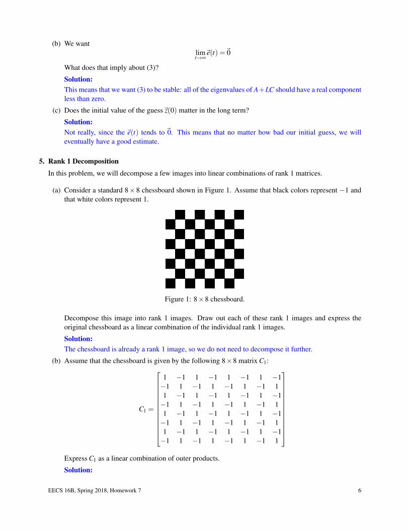
(a) Consider a standard 8×8 chessboard shown in Figure 1. Assume that black colors represent −1 andthat white colors represent 1.

Figure 1: 8×8 chessboard.

Decompose this image into rank 1 images. Draw out each of these rank 1 images and express theoriginal chessboard as a linear combination of the individual rank 1 images.

Solution:The chessboard is already a rank 1 image, so we do not need to decompose it further.

(b) Assume that the chessboard is given by the following 8×8 matrix C1:

C1 =

1 −1 1 −1 1 −1 1 −1−1 1 −1 1 −1 1 −1 11 −1 1 −1 1 −1 1 −1−1 1 −1 1 −1 1 −1 11 −1 1 −1 1 −1 1 −1−1 1 −1 1 −1 1 −1 11 −1 1 −1 1 −1 1 −1−1 1 −1 1 −1 1 −1 1

Express C1 as a linear combination of outer products.

Solution:


Using the result from the previous part,

C1 =

1−11−11−11−1

[1 −1 1 −1 1 −1 1 −1

]

(c) For the same chessboard shown in Figure 1, now assume that black colors represent 0 and that whitecolors represent 1.Decompose this image into rank 1 images. Draw out each of these rank 1 images and express theoriginal chessboard as a linear combination of the individual rank 1 images.

Solution:The chessboard is now a rank 2 image, so we need to decompose it.Image 1:

Image 2:

The chessboard equals the sum of image 1 and image 2.


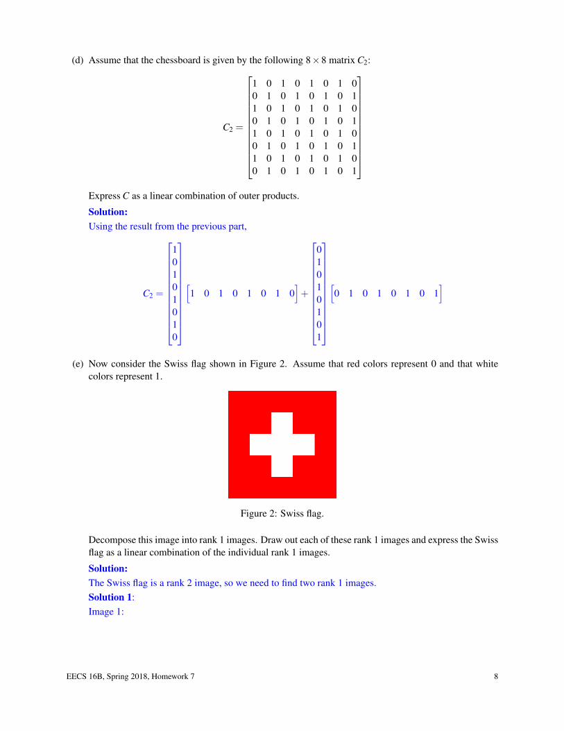
(d) Assume that the chessboard is given by the following 8×8 matrix C2:

C2 =

1 0 1 0 1 0 1 00 1 0 1 0 1 0 11 0 1 0 1 0 1 00 1 0 1 0 1 0 11 0 1 0 1 0 1 00 1 0 1 0 1 0 11 0 1 0 1 0 1 00 1 0 1 0 1 0 1

Express C as a linear combination of outer products.

Solution:Using the result from the previous part,

C2 =

10101010

[1 0 1 0 1 0 1 0

]+

01010101

[0 1 0 1 0 1 0 1

]

(e) Now consider the Swiss flag shown in Figure 2. Assume that red colors represent 0 and that whitecolors represent 1.

Figure 2: Swiss flag.

Decompose this image into rank 1 images. Draw out each of these rank 1 images and express the Swissflag as a linear combination of the individual rank 1 images.

Solution:The Swiss flag is a rank 2 image, so we need to find two rank 1 images.Solution 1:Image 1:


Image 2:

The Swiss flag equals the sum of image 1 and image 2.Solution 2:Image 1:

Image 2:

The Swiss flag equals the difference between image 1 and image 2.


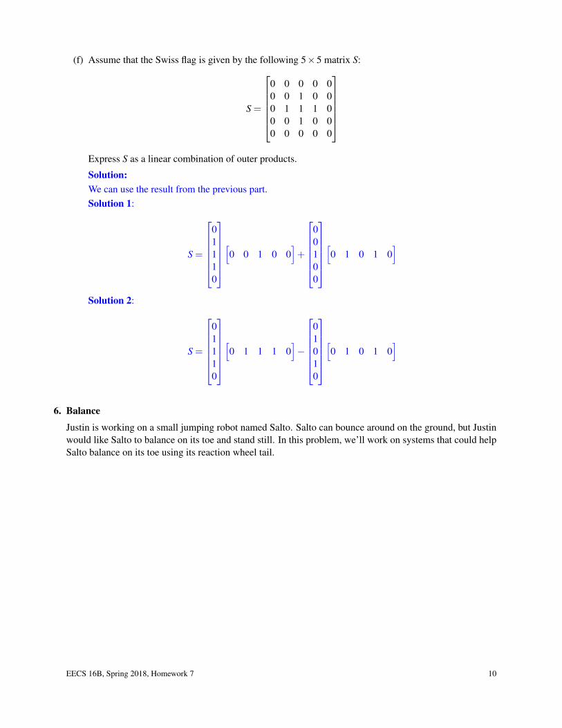
(f) Assume that the Swiss flag is given by the following 5×5 matrix S:

S =

0 0 0 0 00 0 1 0 00 1 1 1 00 0 1 0 00 0 0 0 0

Express S as a linear combination of outer products.

Solution:We can use the result from the previous part.Solution 1:

S =

01110

[0 0 1 0 0

]+

00100

[0 1 0 1 0

]

Solution 2:

S =

01110

[0 1 1 1 0

]−

01010

[0 1 0 1 0

]

6. Balance

Justin is working on a small jumping robot named Salto. Salto can bounce around on the ground, but Justinwould like Salto to balance on its toe and stand still. In this problem, we’ll work on systems that could helpSalto balance on its toe using its reaction wheel tail.


Figure 3: Picture of Salto and the x-z physics model. You can watch a video of Salto here: http://www.youtube.com/watch?v=2dJmArHRn0U

Standing on the ground, Salto’s dynamics in the x-z plane (called the sagittal plane in biology) look like aninverted pendulum with a flywheel on the end:

(I1 +(m1 +m2)l2)θ̈1 =−Ktu+(m1 +m2)lgsin(θ1)

I2θ̈2 = Ktu

where θ1 is the angle of the robot’s body relative to the ground (0 is straight up), θ̇1 is its angular velocity, θ̇2is the angular velocity of the reaction wheel tail, and u is the current input to the tail motor. m1,m2, I1, I2, l,Kt

are positive constants representing system parameters (masses and angular momentums of the body and tail,leg length, and motor torque constant respectively) and g = 9.81 m

s2 is the acceleration due to gravity.

Numerically substituting Salto’s physical parameters, the differential equations become approximately:

0.001θ̈1 =−0.025u+0.1sin(θ1)

5(10−5)θ̈2 = 0.025u

For this problem, we’ll look at a reduced suite of sensors on Salto. Our only output will be the tail encoderthat measures the angular velocity of the tail relative to the body:

y = θ̇2− θ̇1

(a) Using the state vector[θ1 θ̇1 θ̇2

]>, input u, and output y linearize the system about the point[

0 0 0]>

. Write the linearized equations as ddt~x = A~x+Bu and y = C~x. Write out the matrices

with the physical numerical values, not symbolically.Note: Since the tail is like a wheel, we care only about its angular velocity θ̇2 and not its angle θ2.

Solution:


http://www.youtube.com/watch?v=2dJmArHRn0U

http://www.youtube.com/watch?v=2dJmArHRn0U

Numerically, the dynamics are:θ̇1θ̈1θ̈2

=

0 1 0100 0 00 0 0

θ1

θ̇1θ̇2

+ 0−25500

u

y =[0 −1 1

]θ1θ̇1θ̇2

For those interested, the symbolic dynamics are:θ̇1

θ̈1θ̈2

=

0 1 0(m1+m2)lgsin(θ)

I1+(m1+m2)l2 0 00 0 0

θ1

θ̇1θ̇2

+ 0− Kt

I1+(m1+m2)l2

KtI2

u

y =[0 −1 1

]θ1θ̇1θ̇2

(b) Is the system fully controllable? Is the system fully observable?

Solution:

C =[B AB A2B

]=

0 −25 0−25 0 −2500500 0 0

which is full rank, so the system is fully controllable.

O =

CCACA2

=

0 −1 1−100 0 0

0 −100 0

which is rank 3, so the system is fully observable.

(c) Design an observer of the form ddt~̂x = A~̂x+Bu+L(C~̂x− y) and solve for the gains in L that make the

observer dynamics converge with all eigenvalues λ1 = λ2 = λ3 =−10.

Solution:The observer dynamics are dictated by

~̇e = (A+LC)~e

where~e is the error between the estimated state x̂ and the true state~x. The characteristic polynomial is:

det(A+LC) = 0

det

0 1− l1 l1

100 −l2 l20 −l3 l3

= 0

λ3 +(−l3 + l2)λ 2 +(100l1−100)λ +100l3 = 0


The desired characteristic polynomial is:

(λ +10)3 = 0

λ3 +30λ

2 +300λ +1000 = 0

which we can achieve by matching the coefficients of matching powers:

−l3 + l2 = 30

100l1−100 = 300

100l3 = 1000

These equations are solved by the gains: l1 = 4, l2 = 40, and l3 = 10. Written as a matrix,

L =

44010

(d) Let’s implement a controller for our system using an analog electrical circuit! You can use the follow-

ing circuit components in Figure 2:

Figure 4: Circuit components and block diagram symbols.


Using state feedback, Justin has selected the control gains K =[−20 −5 −0.01

]for his input

u = −K~x. Draw a block diagram in the box in Figure 5 that implements this controller. Afterwards,design the circuit that implements the controller. Use relatively reasonable component values.Optional: What are the eigenvalues of the closed loop dynamics for the given K?

Figure 5: Fill in the box to implement the state feedback controller.

Solution:

Figure 6: Here is a possible circuit. Other resistor values will work as long as the gains are the same.

Optional: The eigenvalues are λ =−116.6 and λ =−1.697±1.187 j.


Contributors:

• Edward Wang.

• John Maidens.

• Siddharth Iyer.

• Titan Yuan.

• Justin Yim.


homework 7 - inst.eecs.berkeley.eduee16b/sp18/hw/hw7/sol7.pdf · eecs 16b designing information...

Documents