homework 10 solutions - california state university,...

Homework 10 solutions Section 5.3: Ex 4,5; AP 1,5 Section 5.4: Ex 1,2,3,4; AP 1,3 Section 5.3 4. Find the clamped cubic spline that passes through the points (-3,2), (-2,0), (1,3), and (4,1) with the 1st derivative boundary condition S’(-3) = -1 and S’(4) = 1. h0 = 1, h1 = 3, h2 = 3; d0 = -2, d1 = 1, d2 = -2/3; u1 = 18, u2 = -10, and m0 = -3 – m1/2, m3 = 5/3 – m2/2. Then we solve

!"

!#

$

%=+

=+

152

213

2132

15

21

21

mm

mm

, to get m1 = 118/31 and m2 = -78/31.

Then the cubic spline is

!!!

"

!!!

#

$

%+&+&&&

&%+&+&+&

&&%++&+&+

=

]4,1[3)1(31

12)1(

31

39)1(

837

253

]1,2[)2(31

48)2(

31

59)2(

279

98

]2,3[2)3()3(31

76)3(

31

45

)(

23

23

23

xxxx

xxxx

xxxx

xS

5. Find the natural cubic spline through the points in problem 4. As before, h0 = 1, h1 = 3, h2 = 3; d0 = -2, d1 = 1, d2 = -2/3; u1 = 18, u2 = -10, but now we must enforce the condition S’’(x) = 0 at -3 and 4.

Solve !"#

$=+

=+

10123

1838

21

21

mm

mm, to get m1 = 82/29 and m2 = -134/87.

Set m0 = 0 = m3. The cubic spline is

!!!

"

!!!

#

$

%+&+&&&

&%+&+++&

&&%++&+

=

]4,1[3)1(87

76)1(

87

67)1(

783

67

]1,2[)2(87

92)2(

29

41)2(

783

100

]2,3[2)3(87

215)3(

87

41

)(

23

23

3

xxxx

xxxx

xxx

xS

Algorithms and Programs 1. The distance dk that a car traveled at time tk is given in the following table. Use the clamped spline code with 1st derivative conditions S’(0) = 0 and S’(8) = 98, and find the clamped cubic spline for the points.

Time, tk 0 2 4 6 8 Distance, dk 0 40 160 300 480

One can use the spline code to find the coefficients in the clamped cubic spline. Then to plot the function we need to plot the polynomials between the interpolated points. A code to do this follows the results below.

t = 0:2:8; d = [0 40 160 300 480]; d0 = 0; dn = 98; Sc = csfit(t,d,d0,dn) tt = linspace(min(t),max(t),500); S = 0*tt; for i = 1:(length(t)-1) S = S + ... (Sc(i,4) + Sc(i,3)*(tt-t(i)) + Sc(i,2)*(tt-t(i)).^2 +... Sc(i,1)*(tt-t(i)).^3).*(tt>=t(i)).*(tt<t(i+1)); end S = S + d(i+1)*(tt==t(i+1)); figure(1) plot(t,d,'r*',tt,S,'b')

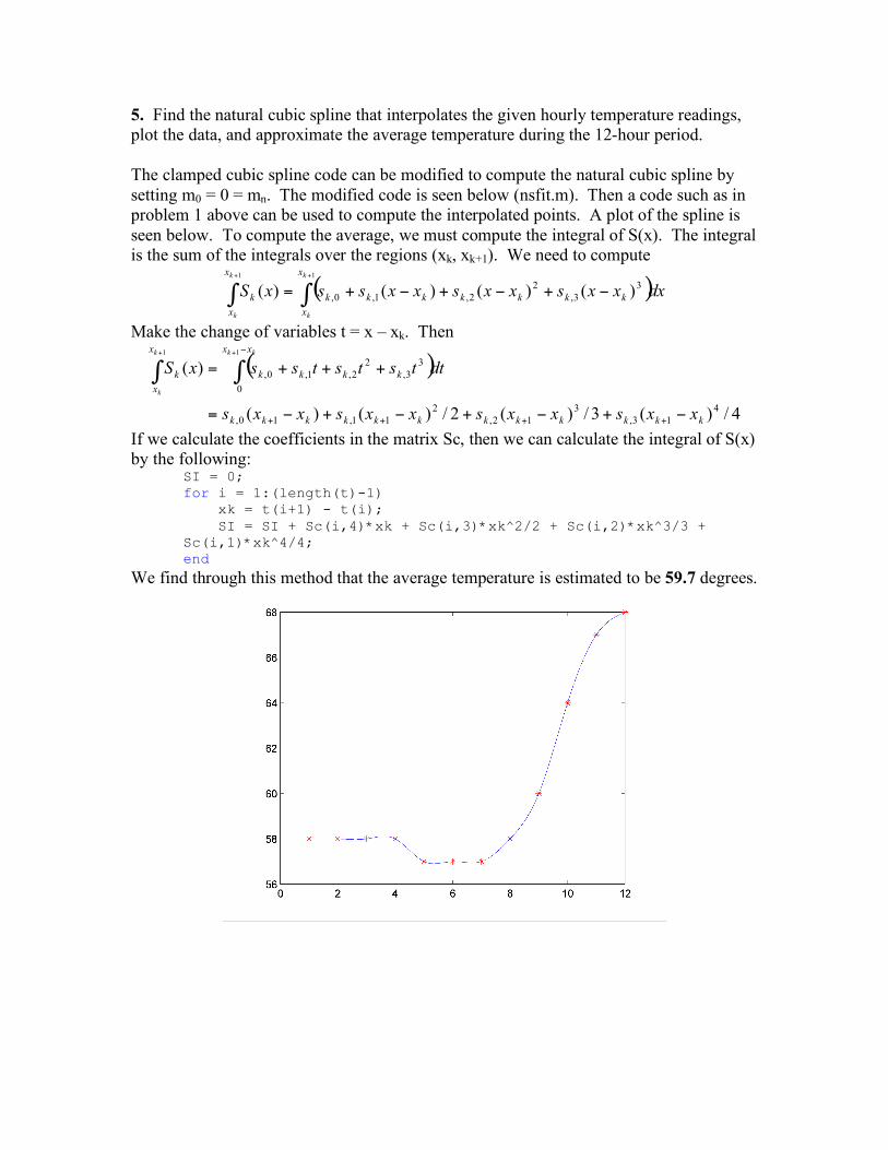
5. Find the natural cubic spline that interpolates the given hourly temperature readings, plot the data, and approximate the average temperature during the 12-hour period. The clamped cubic spline code can be modified to compute the natural cubic spline by setting m0 = 0 = mn. The modified code is seen below (nsfit.m). Then a code such as in problem 1 above can be used to compute the interpolated points. A plot of the spline is seen below. To compute the average, we must compute the integral of S(x). The integral is the sum of the integrals over the regions (xk, xk+1). We need to compute

( )!!++

"+"+"+=11

3

3,

2

2,1,0, )()()()(k

k

k

k

x

x

kkkkkkk

x

x

kdxxxsxxsxxssxS

Make the change of variables t = x – xk. Then

( )

4/)(3/)(2/)()(

)(

4

13,

3

12,

2

11,10,

0

3

3,

2

2,1,0,

11

kkkkkkkkkkkk

xx

kkkk

x

x

k

xxsxxsxxsxxs

dttststssxS

kkk

k

!+!+!+!=

+++=

++++

!

""++

If we calculate the coefficients in the matrix Sc, then we can calculate the integral of S(x) by the following:

SI = 0; for i = 1:(length(t)-1) xk = t(i+1) - t(i); SI = SI + Sc(i,4)*xk + Sc(i,3)*xk^2/2 + Sc(i,2)*xk^3/3 + Sc(i,1)*xk^4/4; end

We find through this method that the average temperature is estimated to be 59.7 degrees.

function S=nsfit(X,Y) %Natural spline interpolation %Input - X is the 1xn abscissa vector % - Y is the 1xn ordinate vector %Output - S: rows of S are the coefficients for the cubic interpolants N=length(X)-1; H=diff(X); D=diff(Y)./H; A=H(2:N-1); B=2*(H(1:N-1)+H(2:N)); C=H(2:N); U=6*diff(D); for k=2:N-1 temp=A(k-1)/B(k-1); B(k)=B(k)-temp*C(k-1); U(k)=U(k)-temp*U(k-1); end M=zeros(N+1); M(N)=U(N-1)/B(N-1); for k=N-2:-1:1 M(k+1)=(U(k)-C(k)*M(k+2))/B(k); end for k=0:N-1 S(k+1,1)=(M(k+2)-M(k+1))/(6*H(k+1)); S(k+1,2)=M(k+1)/2; S(k+1,3)=D(k+1)-H(k+1)*(2*M(k+1)+M(k+2))/6; S(k+1,4)=Y(k+1); end

Section 5.4 1. Find the Fourier series representation and graph the partial sums S2(x), S3(x) and S4(x) of its Fourier series representation for

!"#

<<

<<$$=

%

%

x

xxf

01

01)(

Using the Mathematica program Fourier_Series.nb available on the course website, we find that f(x) = 1.27324 sin(x)+0.424413 sin(3 x)+0.254648 sin(5 x)+0.181891 sin(7 x) + ... The graphs of the partial sums are seen below. The red is f(x), and the blue is (from left to right) S2(x), S3(x), S4(x).

2. Repeat problem 1 for

!"

!#

$

<<%

<<%+

=

&&

&&

xx

xxxf

02

02)(

f(x) = 1.27324 cos(x)+0.141471 cos(3x)+0.0509296 cos(5x)+0.0259845 cos(7x) + ...


!"#

<<

<<$=

%

%

xx

xxf

0

00)(

f(x) = 0.785398 -0.63662 cos(x)-0.0707355 cos(3x)-0.0254648 cos(5x)-0.0129922 cos(7x) + sin(x)-0.5 sin(2x) + 1/3 sin(3x) - 0.25 sin(4x) + 0.2 sin(5x) - 0.166667 sin(6x) + 0.142857 sin(7x) + ...


!!!

"

!!!

#

$

%<<%%

<<%

<<%

=

21

221

21

)(

&&

&&

&&

x

x

x

xf

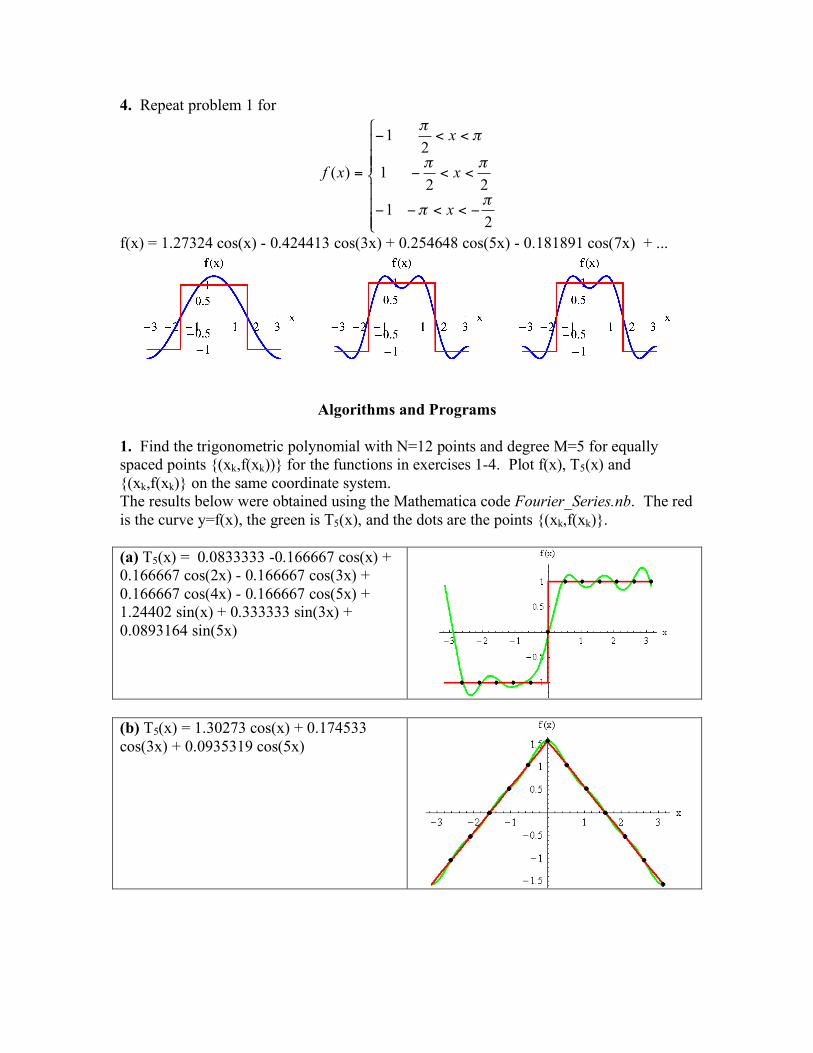
f(x) = 1.27324 cos(x) - 0.424413 cos(3x) + 0.254648 cos(5x) - 0.181891 cos(7x) + ...

Algorithms and Programs 1. Find the trigonometric polynomial with N=12 points and degree M=5 for equally spaced points {(xk,f(xk))} for the functions in exercises 1-4. Plot f(x), T5(x) and {(xk,f(xk)} on the same coordinate system. The results below were obtained using the Mathematica code Fourier_Series.nb. The red is the curve y=f(x), the green is T5(x), and the dots are the points {(xk,f(xk)}. (a) T5(x) = 0.0833333 -0.166667 cos(x) + 0.166667 cos(2x) - 0.166667 cos(3x) + 0.166667 cos(4x) - 0.166667 cos(5x) + 1.24402 sin(x) + 0.333333 sin(3x) + 0.0893164 sin(5x)

(b) T5(x) = 1.30273 cos(x) + 0.174533 cos(3x) + 0.0935319 cos(5x)

(c) T5(x) = 0.916298 -0.913165 cos(x) + 0.261799 cos(2x) - 0.349066 cos(3x) + 0.261799 cos(4x) - 0.308565 cos(5x) + 0.977049 sin(x) - 0.45345 sin(2x) + 0.261799 sin(3x) - 0.15115 sin(4x) + 0.0701489 sin(5x)

(d) T5(x) = 0.0909091 + 1.27758 cos(x) - 0.189494 cos(2x) - 0.437678 cos(3x) + 0.216128 cos(4x) + 0.277644 cos(5x)

3. Modify your code so that it will find the trigonometric polynomial on [a, b]. Once we know how to find TM(x) on [-π, π], we can find the polynomial on any interval [a, b] by making the following transformation:

22

bay

abx

++

!=

".

Then x is in [a, b] and y is in [-π, π]. So find the trig polynomial for

!"

#$%

& ++

'=

22)(

bay

abfxf

(.

Then we get TM(y), and to get TM(x) we take

!"

#$%

&

'

+'

'=

ab

bay

abTxT MM

)(2)(

(( .

The mathematica code Fourier_Series.nb on the course website will perform such a translation.

homework 10 solutions - california state university,...

Documents