homer help manual - science.smith.edu · homer (hybrid optimization of multiple electric...
TRANSCRIPT

1/16/2015 HOMER Help Manual
file:///C:/users/jonathan/documents/HOMER_help/HOMERManual_SourceCode_output/SingleHTML/HOMER.htm 1/241
HOMER Help ManualTable of contents
1. Welcome to HOMER 1.1 Solving Problems with HOMER 1.2 The HOMER Knowledgebase 1.3 HOMER Professional Quick Start Guide 1.4 Addon Modules2. Navigating HOMER 2.1 Loads Tab 2.1.1 Adding a Load to the Model 2.1.2 Load Profile Menu 2.1.2.1 Efficiency 2.1.3 Electric Load 2.1.4 Thermal Load 2.1.5 Deferrable Load 2.1.6 Hydrogen Load 2.2 Components Tab 2.2.1 Generator 2.2.1.1 Fuel Curve 2.2.2 PV (Photovoltaic) 2.2.3 Wind Turbine 2.2.4 Battery 2.2.5 Flywheel 2.2.6 Converter 2.2.7 Boiler 2.2.8 Hydro 2.2.8.1 Pipe Head Loss Calculator 2.2.9 Hydrokinetic 2.2.10 Thermal Load Controller 2.2.11 Grid 2.2.11.1 Simple rates 2.2.11.2 Real time prices 2.2.11.3 Scheduled rates 2.2.11.4 Grid extension 2.2.12 Hydrogen Tank 2.2.13 Electrolyzer 2.2.14 Reformer 2.3 Resources 2.3.1 Solar GHI Resource 2.3.2 Solar DNI Resource 2.3.3 Temperature Resource 2.3.4 Wind Resource 2.3.4.1 Wind Resource Parameters 2.3.4.2 Wind Resource Variation with Height 2.3.4.3 Wind Resource Advanced Parameters 2.3.5 Hydro Resource 2.3.6 Fuel Resource 2.3.7 Biomass Resource 2.3.8 Hydrokinetic 2.4 System Tab 2.4.1 Project Set Up 2.4.1.1 Economics 2.4.1.2 System Control 2.4.1.3 Emissions 2.4.1.4 Constraints 2.4.2 Input Report 2.4.3 Search Space 2.4.4 Sensitivity Inputs 2.4.5 Estimate 2.5 Design View 2.6 Calculate Button 2.7 Results View 2.7.1 Simulation Results 2.7.1.1 Cost Summary Outputs 2.7.1.1.1 Compare Economics Window 2.7.1.1.2 Calculating Payback, Internal Rate of Return (IRR) and Other Economic Metrics 2.7.1.1.3 Grid Costs 2.7.1.2 Cash Flow Outputs 2.7.1.3 Electrical Outputs 2.7.1.4 PV Outputs 2.7.1.5 Wind Turbine Outputs 2.7.1.6 Generator Outputs 2.7.1.7 Battery Outputs 2.7.1.8 Grid Outputs

1/16/2015 HOMER Help Manual
file:///C:/users/jonathan/documents/HOMER_help/HOMERManual_SourceCode_output/SingleHTML/HOMER.htm 2/241
2.7.1.9 Converter Outputs 2.7.1.10 Emissions Outputs 2.7.1.11 Thermal Outputs 2.7.1.12 Boiler Outputs 2.7.1.13 Hydro Outputs 2.7.1.14 Time Series Outputs 2.7.1.15 Hydrogen Outputs 2.7.1.16 Hydrogen Tank Outputs 2.7.1.17 Electrolyzer Outputs 2.7.1.18 Report Summarizing the Simulation Results 2.7.2 Optimization Results 2.7.3 Sensitivity Results 2.7.3.1 Why would I do a sensitivity analysis? 2.7.3.2 Adding Sensitivity Values 2.8 Library View 2.8.1 Components 2.8.1.1 Battery 2.8.1.1.1 Vanadium Battery 2.8.1.1.2 Zinc Battery 2.8.1.2 Generator 2.8.1.3 PV 2.8.1.4 Wind Turbine 2.8.1.5 Flywheel 2.8.2 Resources 2.8.2.1 Create a New Fuel 2.8.3 Grid 2.8.4 Simulation Parameters3. HOMER's Calculations 3.1 How HOMER Calculates the PV Array Output 3.2 Beacon Power Smart Energy 25 Flywheel 3.3 How HOMER Calculates Emissions 3.4 How HOMER Calculates the Hydro Power Output 3.5 How HOMER Calculates Clearness Index 3.6 How HOMER Calculates the Maximum Battery Charge Power 3.7 How HOMER Calculates the Maximum Battery Discharge Power 3.8 How HOMER Calculates the Radiation Incident on the PV Array 3.9 How HOMER Calculates Wind Turbine Power Output 3.10 Operation of a Cofired Generator 3.11 How HOMER Creates the Generator Efficiency Curve 3.12 Kinetic Battery Model 3.13 Generating Synthetic Load Data 3.14 Generating Synthetic Solar Data 3.15 Generating Synthetic Wind Data 3.16 Unit Conversions4. Finding data to run HOMER 4.1 US Grid Emissions Factors 4.2 Published Solar Data 4.3 Wind Data Histograms 4.4 Wind Data Parameters 4.5 References 4.6 Recommended Reading5. License Management6. Glossary 6.1 EnglishSpanish Glossary 6.2 Absolute State of Charge 6.3 AC Primary Load Served 6.4 Altitude 6.5 Anemometer Height 6.6 Annualized Cost 6.7 Autocorrelation 6.8 Available Head 6.9 Battery Bank Autonomy 6.10 Battery Bank Life 6.11 Battery Charge Efficiency 6.12 Battery Discharge Efficiency 6.13 Battery Energy Cost 6.14 Battery Float Life 6.15 Battery Maximum Charge Rate 6.16 Battery Minimum State Of Charge 6.17 Battery Roundtrip Efficiency 6.18 Battery Throughput 6.19 Battery Wear Cost 6.20 Biogas (PRO) 6.21 Biomass Carbon Content (PRO) 6.22 Biomass Gasification Ratio (PRO) 6.23 Biomass Resource Cost (PRO) 6.24 Biomass Substitution Ratio (PRO)

1/16/2015 HOMER Help Manual
file:///C:/users/jonathan/documents/HOMER_help/HOMERManual_SourceCode_output/SingleHTML/HOMER.htm 3/241
6.25 Boiler Marginal Cost (PRO) 6.26 Breakeven Grid Extension Distance (PRO) 6.27 Capacity Shortage 6.28 Capacity Shortage Fraction 6.29 Capacity Shortage Penalty 6.30 Capital Recovery Factor 6.31 How HOMER Calculates the PV Cell Temperature 6.32 Clearness Index 6.33 CO Emissions Penalty (PRO) 6.34 CO2 Emissions Penalty 6.35 Component 6.36 Component Library 6.37 Cycle Charging Strategy 6.38 DC Primary Load Served 6.39 Decision Variable 6.40 Deferrable Load Served (PRO) 6.41 Deltaplot 6.42 Design Flow Rate (PRO) 6.43 Discount Factor 6.44 Dispatch Strategy 6.45 Diurnal Pattern Strength 6.46 DMap 6.47 Effective Head (PRO) 6.48 Electrolyzer Efficiency (PRO) 6.49 Excess Electricity 6.50 Excess Electricity Fraction 6.51 Feasible and Infeasible Systems 6.52 Flow Rate Available To Hydro Turbine (PRO) 6.53 Fossil Fraction (PRO) 6.54 Fuel Carbon Content 6.55 Fuel Price 6.56 Fuel Sulfur Content 6.57 Future Value 6.58 Generator 6.59 Generator Average Electrical Efficiency 6.60 Generator Average Total Efficiency 6.61 Generator Carbon Monoxide Emissions Factor 6.62 Generator Derating Factor (PRO) 6.63 Generator Fuel Cost 6.64 Generator Fuel Curve Intercept Coefficient 6.65 Generator Fuel Curve Slope 6.66 Generator Heat Recovery Ratio (PRO) 6.67 Generator Hourly Replacement Cost 6.68 Generator Lifetime 6.69 Generator Minimum Fossil Fraction (PRO) 6.70 Generator Minimum Percent Load 6.71 Generator Nitrogen Oxides Emissions Factor 6.72 Generator Operational Life 6.73 Generator Particulate Matter Emissions Factor 6.74 Generator Proportion of Sulfur Emitted as Particulate Matter 6.75 Generator Unburned Hydrocarbons Emissions Factor 6.76 Grid Costs 6.77 Grid Interconnection Charge (PRO) 6.78 Grid Standby Charge (PRO) 6.79 Ground Reflectance 6.80 Hydrocarbons Emissions Penalty (PRO) 6.81 Hour of Peak Windspeed 6.82 Hydro Turbine Efficiency (PRO) 6.83 Hydro Turbine Flow Rate (PRO) 6.84 Hydrogen Tank Autonomy (PRO) 6.85 Initial Capital Cost 6.86 Interest Rate 6.87 Levelized Cost of Energy 6.88 Lifetime Throughput 6.89 Load Factor 6.90 Load Following Strategy 6.91 Maximum Annual Capacity Shortage 6.92 Maximum Battery Capacity 6.93 Maximum Flow Rate (PRO) 6.94 Maximum Flow Ratio (PRO) 6.95 Purchase Capacity 6.96 Minimum Flow Rate (PRO) 6.97 Minimum Flow Ratio (PRO) 6.98 Net Present Cost 6.99 Nominal Battery Capacity 6.100 Nominal Hydro Power (PRO) 6.101 Nonrenewable Electrical Production

1/16/2015 HOMER Help Manual
file:///C:/users/jonathan/documents/HOMER_help/HOMERManual_SourceCode_output/SingleHTML/HOMER.htm 4/241
6.102 Nonrenewable Thermal Production (PRO) 6.103 NOx Emissions Penalty (PRO) 6.104 O&M (Operation and Maintenance) Cost 6.105 OneHour Autocorrelation Factor 6.106 Operating Capacity 6.107 Operating Cost 6.108 Operating Reserve 6.109 Other Capital Cost 6.110 Other O&M Cost 6.111 Pipe Head Loss (PRO) 6.112 PM Emissions Penalty (PRO) 6.113 Present Value 6.114 Probability Transformation 6.115 Project Lifetime 6.116 PV Azimuth 6.117 PV Derating Factor 6.118 PV Efficiency at Standard Test Conditions (PRO) 6.119 PV Nominal Operating Cell Temperature (PRO) 6.120 PV Slope 6.121 PV Temperature Coefficient of Power (PRO) 6.122 PV Tracking System (PRO) 6.123 Reformer Efficiency (PRO) 6.124 Relative State of Charge 6.125 Renewable Electrical Production 6.126 Renewable Fraction 6.127 Renewable Penetration 6.128 Renewable Thermal Production (PRO) 6.129 Replacement Cost 6.130 Required Operating Capacity 6.131 Required Operating Reserve 6.132 Residual Flow (PRO) 6.133 Resource 6.134 Return On Investment 6.135 Salvage Value 6.136 Search Space 6.137 Sensitivity Analysis 6.138 Sensitivity Case 6.139 Sensitivity Variable 6.140 Setpoint State of Charge 6.141 Simulation Time Step 6.142 Sinking Fund Factor 6.143 SO2 Emissions Penalty (PRO) 6.144 Solar Absorptance 6.145 Solar Transmittance 6.146 Specific Fuel Consumption 6.147 Standard Test Conditions 6.148 Suggested Lifetime Throughput 6.149 System 6.150 System Fixed Capital Cost 6.151 System Fixed Operations and Maintenace (O&M) Cost 6.152 System Roundtrip Efficiency 6.153 Thermal Load Served (PRO) 6.154 Total Annualized Cost 6.155 Total Capacity Shortage 6.156 Total Electrical Load Served 6.157 Total Electrical Production 6.158 Total Thermal Production (PRO) 6.159 Total Excess Electricity 6.160 Total Fuel Cost 6.161 Total Net Present Cost 6.162 Total Unmet Load 6.163 Unmet Load 6.164 Unmet Load Fraction 6.165 Weibull Distribution 6.166 Weibull k Value 6.167 Wind Turbine Hub Height
1. Welcome to HOMER
Welcome to HOMER

1/16/2015 HOMER Help Manual
file:///C:/users/jonathan/documents/HOMER_help/HOMERManual_SourceCode_output/SingleHTML/HOMER.htm 5/241
What is HOMER?HOMER (Hybrid Optimization of Multiple Electric Renewables), the micropower optimization model, simplifies the task of evaluating designs of both offgrid andgridconnected power systems for a variety of applications. When you design a power system, you must make many decisions about the configuration of thesystem: What components does it make sense to include in the system design? How many and what size of each component should you use? The large number oftechnology options and the variation in technology costs and availability of energy resources make these decisions difficult. HOMER's optimization and sensitivityanalysis algorithms make it easier to evaluate the many possible system configurations.
How do I use HOMER?To use HOMER, you provide the model with inputs, which describe technology options, component costs, and resource availability. HOMER uses these inputs tosimulate different system configurations, or combinations of components, and generates results that you can view as a list of feasible configurations sorted by netpresent cost. HOMER also displays simulation results in a wide variety of tables and graphs that help you compare configurations and evaluate them on theireconomic and technical merits. You can export the tables and graphs for use in reports and presentations.
When you want to explore the effect that changes in factors such as resource availability and economic conditions might have on the costeffectiveness of differentsystem configurations, you can use the model to perform sensitivity analyses. To perform a sensitivity analysis, you provide HOMER with sensitivity values thatdescribe a range of resource availability and component costs. HOMER simulates each system configuration over the range of values. You can use the results of asensitivity analysis to identify the factors that have the greatest impact on the design and operation of a power system. You can also use HOMER sensitivityanalysis results to answer general questions about technology options to inform planning and policy decisions.
How does HOMER work?
SimulationHOMER simulates the operation of a system by making energy balance calculations in each time step of the year. For each time step, HOMER compares theelectric and thermal demand in that time step to the energy that the system can supply in that time step, and calculates the flows of energy to and from eachcomponent of the system. For systems that include batteries or fuelpowered generators, HOMER also decides in each time step how to operate the generatorsand whether to charge or discharge the batteries.
HOMER performs these energy balance calculations for each system configuration that you want to consider. It then determines whether a configuration isfeasible, i.e., whether it can meet the electric demand under the conditions that you specify, and estimates the cost of installing and operating the system over thelifetime of the project. The system cost calculations account for costs such as capital, replacement, operation and maintenance, fuel, and interest.
OptimizationAfter simulating all of the possible system configurations, HOMER displays a list of configurations, sorted by net present cost (sometimes called lifecycle cost), thatyou can use to compare system design options.
Sensitivity AnalysisWhen you define sensitivity variables as inputs, HOMER repeats the optimization process for each sensitivity variable that you specify. For example, if you definewind speed as a sensitivity variable, HOMER will simulate system configurations for the range of wind speeds that you specify.
For more informationThe HOMER Support Site has a searchable knowledgebase and additional support options.
HOMER online contains the latest information on model updates, as well as sample files, resource data, and contact information.
© 20122014 HOMER Energy, LLCLast modified: Sept 28, 2012
[TOP]
1.1 Solving Problems with HOMER
Solving Problems with HOMER
HOMER simplifies the task of designing distributed generation (DG) systems both on and offgrid. HOMER's optimization and sensitivity analysis algorithms allow

1/16/2015 HOMER Help Manual
file:///C:/users/jonathan/documents/HOMER_help/HOMERManual_SourceCode_output/SingleHTML/HOMER.htm 6/241
you to evaluate the economic and technical feasibility of a large number of technology options and to account for variations in technology costs and energy resourceavailability.
Working effectively with HOMER requires understanding of its three core capabilities simulation, optimization, and sensitivity analysis and how they interact.
Simulation, Optimization, Sensitivity AnalysisSimulation: At its core, HOMER is a simulation model. It will attempt to simulate a viable system for all possible combinations of the equipment that you wish toconsider. Depending on how you set up your problem, HOMER may simulate hundreds or even thousands of systems.
Optimization: The optimization step follows all simulations. The simulated systems are sorted and filtered according to criteria that you define, so that you can seethe best possible fits. Although HOMER fundamentally is an economic optimization model, you may also choose to minimize fuel usage.
Sensitivity analysis: This is an optional step that allows you to model the impact of variables that are beyond your control, such as wind speed, fuel costs, etc, andsee how the optimal system changes with these variations.
HOMER models both conventional and renewable energy technologies:
Power sources in HOMER:• solar photovoltaic (PV)• wind turbine• generator: diesel• electric utility grid• runofriver hydro power• biomass power• generator: gasoline, biogas,alternative and custom fuels,cofired• microturbine• fuel cell
Storage in HOMER:• flywheels• customizable batteries• flow batteries• hydrogen
Loads in HOMER:• get started quickly with theHOMER Quick Load Builder• daily profiles with seasonalvariation• deferrable (water pumping,refrigeration)• thermal (space heating, cropdrying)• efficiency measures
See also:
Simulation Results
Optimization Results
Sensitivity Results
For more informationThe HOMER Support Site has a searchable knowledgebase and additional support options.
HOMER online contains the latest information on model updates, as well as sample files, resource data, and contact information.
© 20122014 HOMER Energy, LLCLast modified: Nov. 27, 2013
[TOP]
1.2 The HOMER Knowledgebase
Knowledgebase
The Knowledgebase is a searchabale database of questions from HOMER users concerning system modeling, training, downloads and licensing. Questions areaddressed by HOMER support experts.
The Knowledgebase can be accessed online at http://support.homerenergy.com/index.php?/Knowledgebase/List
For more informationThe HOMER Support Site has a searchable knowledgebase and additional support options.
HOMER online contains the latest information on model updates, as well as sample files, resource data, and contact information.
© 20122014 HOMER Energy, LLCLast modified: July 1, 2013
[TOP]
1.3 HOMER Professional Quick Start Guide

1/16/2015 HOMER Help Manual
file:///C:/users/jonathan/documents/HOMER_help/HOMERManual_SourceCode_output/SingleHTML/HOMER.htm 7/241
Quick Start Tutorial
HOMER® Professional can help you design the best micropower system to suit your needs.With HOMER Professional, you can:
Evaluate offgrid or gridconnected system designsChoose the best system based on cost, technical requirements, or environmental considerations.Simulate many design configurations under market price uncertainty and evaluate riskChoose the best addition or retrofit for an existing system
This worked example is intended to get you started in HOMER Professional quickly by walking through one way to run an analysis. It is not intended to replace thestudy of how power systems operate or to cover all areas of HOMER. It should provide you with basic familiarity of the interface.
Step 1. Open HOMER Professional. A new project will display. Enter title, author, or notes if desired. Notice the Component, Load, and Resources tabs at the topof the screen. These allow you to navigate through the model. The load tab will be displayed at startup.
Step 2. Switch to the Components tab. Select “Generator” from the component menu. Select "100 kW Genset" from the dropdown menu and click "AddGenerator".The generator specification menu will display and an icon will appear on the AC bus in the schematic on the left. In the costs table, enter the followingvalues:
Size (kW) 1; Capital ($) 1500; Replace ($) 1200; and O&M ($/hr) 0.05
This tells HOMER that the generator initially costs $1,500 per kilowatt, costs $1,200 per kilowatt to replace at the end of life, and costs $0.05 per hour to operateand maintain (excluding fuel).
Step 3. In the Search Space table, change “Size (kW)” from 100 to 15. Change “Fuel Price ($/L)” to 0.4.
Step 4. Now choose “Wind Turbine” from the components menu. From the dropdown menu on the landing page, choose “Generic 10 kW”. Click "Add WindTurbine". In the costs table, enter:
Size (kW) 1; Capital ($) 30000; Replace ($) 25000; O&M ($/yr) 500
Step 5. Similarly, add a battery from the components menu and choose “Generic 1 kWh Lead Acid”. Set the costs table values to: Size (kW) 1; Capital ($) 300;Replace ($) 300; O&M ($/yr) 20. Change the number of batteries under “Search Space” to 8.
Step 6. Pick the Load tab at the top of the window and choose “Electric #1”. Use option 1: Create a synthetic load from a profile. Leave “Residential” selected andset the “Peak Month” to July. Click “Ok”.

1/16/2015 HOMER Help Manual
file:///C:/users/jonathan/documents/HOMER_help/HOMERManual_SourceCode_output/SingleHTML/HOMER.htm 8/241
Step 7. A load specification menu should display similar to the image below. Change the “Scaled Annual Average (kWh/day)” to 50.
Step 8. The schematic on the left side of the window should now look like this:
Step 9. Now you will specify the details of the wind resource. Select the “Resources” tab at the top and pick “Wind”. You can enter monthly wind data manually orload it from a file. For the purpose of this example, manually enter 1 for all months below “Average Wind Speed (m/s)”. Then change the “Scaled Annual Average(m/s)” to 4.

1/16/2015 HOMER Help Manual
file:///C:/users/jonathan/documents/HOMER_help/HOMERManual_SourceCode_output/SingleHTML/HOMER.htm 9/241
Step 10. Set “Anemometer Height (m)” to 25 to indicate that the specified wind speed (in this case 4 m/s avg.) is as measured at 25 m above ground level.
Step 11. Click “Calculate”.
Step 12. An error will be generated. That is because you need a converter to allow power to flow between the AC bus and the DC bus for the system to function.
Step 13. Select the Components tab and add a converter. Set the capital cost to $1000 and the replacement cost to $1000. Set the operations and maintenancecost to 100 $/yr. In the search space table, add the values 0, 6, and 12 for Size (kW).
Step 14. Now calculate again. The results will display. The upper table shows the best design for each case. In this optimization there is only one case. A systemwith a 6 kW converter is the lowest net present cost design. The lower table displays all configurations that were simulated for this single case – a system with a 6kW converter and one with a 12 kW converter. The system with a 0 kW converter is not displayed since it is not feasible.
Step 15. Now that you have generated some simple results, you can go back and add additional system configurations (called “Search Space”) and input variablevalues (i.e. fuel price; this is called “Sensitivity Analysis”) to your optimization.
Return to the design menu:
Step 16. Select the battery icon in the schematic. Add more values to the quantity search space: 8, 16, 24.
Step 17. Do the same for the wind turbine search space: 0, 1, 2.

1/16/2015 HOMER Help Manual
file:///C:/users/jonathan/documents/HOMER_help/HOMERManual_SourceCode_output/SingleHTML/HOMER.htm 10/241
Step 18. For the generator, enter 10, 15, and 20 kW in the search space.
Step 19. These three variables (number of batteries, number of wind turbines, and size of generator) are configurations in the Search Space. We can also addsensitivity variables to see the effect of different environmental or economic variations. In the generator menu, click the down arrow next the “Fuel Price” and in thetable that appears, enter 0.6, 0.8, 1.2, 1.8 and 2.6 $/L.
Step 20. Similarly, we can check the impact of a larger or smaller load on our costs and optimal system configuration. In the load menu, click the down arrow nextto "Scaled Annual Average (kWh/day)" and enter 30, 50, and 80 kWh/d.
Step 20. At the top of the window, choose the “Resources” tab and select “Wind”. Click the down arrow next to “Scaled Annual Average (m/s)” and enter 2, 4, and6.
Step 21. Press calculate again. HOMER will run a few thousand simulations, and the results tables will display. In the upper table, each row corresponds to onesensitivity case. For each case, the configuration for the lowest net present cost system is listed. Click on the column headings to sort by the different parameters. Ifyou select a sensitivity case, the lower table will show all system configurations that were simulated for that case. Infeasible system configurations are not included.
In the image below, the sensitivity cases in the top table are sorted by number of batteries. The case with 0.80 $/L fuel cost, 30 kWh/day average load, and 6 m/saverage wind speed is selected. The winning system configuration for this case is listed in the top table: One G10 (general 10 kW) wind turbine, a 10 kW generator,24 batteries (1 kWh lead acid), and a 6 kW converter.
In the lower table, all the simulation results for this case with different system configurations are shown, sorted by net present cost. The top row is the samewinning system configuration that is listed in the upper table. The second row reports simulation results from a system with 16 batteries instead of 24. The initialcapital cost decreases from $58,200 to $55,800, but the operating cost increases from $4,841 to $5,117, resulting in a higher net present cost.
Step 22. Above and to the right of the table in the results window is the option to switch to a graphic results display. Set the Fuel Cost to display on the xaxis andWind Speed to display on the yaxis. Set the Avg. Load to 30 (kWh/day). The colors describe the optimal system configuration: in this optimization, the wind turbineis beneficial with higher average wind speeds and higher fuel cost (green shading). At lower wind speeds and fuel costs, the system configuration without the windturbine (blue) yields a lower net present cost.
Double click on a system to view detailed simulation results. You can change the economic variables that determine net present cost, the optimal system selectioncriteria (lowest cost, weight, or fuel use), and other optimization settings in the Project menu:
For more informationThe HOMER Support Site has a searchable knowledgebase and additional support options.
HOMER online contains the latest information on model updates, as well as sample files, resource data, and contact information.
© 20122014 HOMER Energy, LLCLast modified: Sept 28, 2012
[TOP]
1.4 Addon Modules
Modules

1/16/2015 HOMER Help Manual
file:///C:/users/jonathan/documents/HOMER_help/HOMERManual_SourceCode_output/SingleHTML/HOMER.htm 11/241
Several addon modules are available that add advanced functionality to HOMER Pro. New modules will become available as they are developed. The table belowlists the currently available modules.
Module FeaturesBiomass Biomass resource, biogas fuel, biogas and cofired generator.
Hydro Hydro component and hydro resource.
Combined Heat and Power Thermal load, boiler, thermal load controller, and generator heat recovery ratio.
Advanced Load Additional electric load and deferrable load.
For more informationThe HOMER Support Site has a searchable knowledgebase and additional support options.
HOMER online contains the latest information on model updates, as well as sample files, resource data, and contact information.
© 20122014 HOMER Energy, LLCLast modified: July 1, 2013
[TOP]
2. Navigating HOMER
Navigating HOMER
HOMER has three project views: Design, Results, and Library. When you first open HOMER, or when you load a new or existing project, the Home page isdisplayed.
The Design view is the next step. You can use the Load, Components, and Resources tabs to build your system while in the Design view. You can also use theSystem tab to change project parameters, check inputs, and change sensitivity and optimization variables.
Finally, when you click calculate, you will be taken to the Results view (also accessible from the Results button). Here you can review and plot the senstivity cases,investigate optimal systems, and review the details of individual simulations.
The Library button accesses your library, where you can save definitions for components, resources, loads, grid connections, and simulation configurations.
HomeWhen you open a file or start a new project, HOMER displays the Home page. On the Home page, you can display and edit metadata describing your projectincluding project author, title and description. You can also assign a location for you project with the map. If you plan to add PV to you system, picking a locationwhile on the Home page can streamline the process of adding PV and a solar resource.
For more informationThe HOMER Support Site has a searchable knowledgebase and additional support options.
HOMER online contains the latest information on model updates, as well as sample files, resource data, and contact information.
© 20122014 HOMER Energy, LLCLast modified: Nov. 26, 2013
[TOP]
2.1 Loads Tab
Loads Tab
The Loads tab contains primary (electrical), thermal, and deferrable loads. This help topic explains several aspects of the process of specifying a load:
Adding a Load to the Model Instructions on how to add a loadLoad Profile Menu Change load specifications after the load is added to the modelPrimary Load, Thermal Load, Deferrable Load, Hydrogen Load More details on each load type

1/16/2015 HOMER Help Manual
file:///C:/users/jonathan/documents/HOMER_help/HOMERManual_SourceCode_output/SingleHTML/HOMER.htm 12/241
For more informationThe HOMER Support Site has a searchable knowledgebase and additional support options.
HOMER online contains the latest information on model updates, as well as sample files, resource data, and contact information.
© 20122014 HOMER Energy, LLCLast modified: July 2, 2013
[TOP]
2.1.1 Adding a Load to the Model
Adding a Load to the Model
You can add electric or thermal load data using exactly the same process, described here. Measured load data is seldom available, so users often synthesize loaddata by specifying typical daily load profiles and then adding in some randomness. This process produces one year of hourly load data.
Electric Load Set UpHOMER provides four methods to specify an electric load profile.
Create a synthetic load from a profile.This is a quick way to generate a load that can be relatively realistic. If you would like the load to have a cyclic annual variation, you can choose "January" or"July" as the peak month. Choosing "None" will yield an annual profile that is uniform except for random variation.
Peak Month: January Peak Month: July Peak Month: None
The dropdown menu contains a few preset load profiles: Residential, Commercial, Industrial, Community, and Blank. Blank is an empty template.
Residential Commercial
Industrial Community

1/16/2015 HOMER Help Manual
file:///C:/users/jonathan/documents/HOMER_help/HOMERManual_SourceCode_output/SingleHTML/HOMER.htm 13/241
These load templates all have different default overall magnitudes: 11.35, 2620, 24000, and 170 kWh/day respectively. You can easily scale the average loadof any of them to fit your application by changing the value for "Scaled Annual Average (kWh/day)".
Import a load from a time series file.
To import a file, you must prepare a text file that contains the electric load in each time step for a complete year.
Tip: You can import data with any time step down to one minute. HOMER detects the time step when you import the data file. For example, if the data filecontains 8760 lines, HOMER will assume that it contains hourly data. If the data file contains 52,560 lines, HOMER will assume that it contains 10minutedata.
The data file must contain a single value on each line, where each line corresponds to one time step. Each value in the file represents the average load (inkW) for that time step. The first time step starts at midnight on January 1st. A sample input file appears below.
When you import data from a text file, HOMER makes a copy of the data set and integrates it with the HOMER (.hmr) file. Once the data is part of theHOMER file, HOMER no longer refers to the original text file. If you modify data in the original file, you must import the modified file in order for themodification to be included in the HOMER file. After you import a data file, HOMER calculates the average 24hour load profile for the whole year displays itin the table and graph. HOMER also displays the name of the imported data file in the title of the load profile graph.
If you click Enter daily load profile(s) after importing data from a file, HOMER discards the data from the imported file and synthesizes new data based on thetwelve monthly average load profiles it calculated from the imported data. You can edit synthesized data by selecting the month and changing values in theload profile table. To edit values from an imported file, you must edit the file directly and then import the modified file, as described above.
Build a synthetic load using measured data.
You can import load data for specific devices as a CSV file with 24 hours of data, either in hourly or minuteresolution. Refer to the chart below forappropriate formatting. The first row and first two columns are ignored, reserved for user row titles if desired. The second row (column 3 and onward,highlighted below in yellow) should contain descriptive names for each device. Row 3 through row 1442 (or row 3 through 26 for hourly data, below inorange) contains the load profile for each device in watts.
Note that HOMER will accept a mix of 1440row and 24row data columns in a single document. HOMER will infer the time step based on the number ofrows of data for each column individually.

1/16/2015 HOMER Help Manual
file:///C:/users/jonathan/documents/HOMER_help/HOMERManual_SourceCode_output/SingleHTML/HOMER.htm 14/241
Select the "Open Equipment Database" button in the upper right corner of the Load Designer menu, choose "Open...", and select your csv file. The loaddesigner will import each column in the file as a separate device. You can drag and drop rows from the Equipment Database popup into the Load Designer.Once you are done, close the Equipment Database popup. You can now edit the quantities of each item, if desired. You can also set the "Jitter", whichoffsets the load profiles randomly so that load peaks in the duplicate devices (if set to quantity greater than one) will not always line up exactly.
Choose a load from the library.Choose this option to retrieve load profiles from the HOMER Library.
For more informationThe HOMER Support Site has a searchable knowledgebase and additional support options.
HOMER online contains the latest information on model updates, as well as sample files, resource data, and contact information.
© 20122014 HOMER Energy, LLCLast modified: July 23, 2014
[TOP]
2.1.2 Load Profile Menu
Load Profile Menu
Once you have created a load using one of the methods offered by the Load Set Up, you will be taken to the Load Profile Menu. You can return to this page byclicking on the corresponding load icon in the system schematic or through the Load tab at the top of the HOMER window. The options for electric and thermalloads are similar.
The load profile menu displays the load profile graphically and presents summary statistics for the data. You can modify some details of the load in this menu.
Hourly DataYou can modify the daily profile, hourbyhour in the table on the left side of the menu.
By clicking on "Show All Months..." you can set a different daily profile for weekends and weekdays and for each month of the year.

1/16/2015 HOMER Help Manual
file:///C:/users/jonathan/documents/HOMER_help/HOMERManual_SourceCode_output/SingleHTML/HOMER.htm 15/241
If you select "Copy Changes to Right", any value you enter will be copied across all remaining months. For example, if you enter "10" for January, hour 0, then allmonths, hour 0, will be set to 10. If you then enter "9" for hour 0 in Februrary, January will stay set to 10 and February through December will be set to 9. You canedit values for weekends or for weekdays by selecting the tab at the top of the table. Changes made to the profile for weekends do not affect the profile forweekdays, and vice versa.
Random variabilityRandom variability is defined with two values, "Daytoday" and "Timestep". If you have imported timeseries load data, these values will be listed for reference andwill not be editable. If you are generating synthetic load with HOMER, you can change these values.
The random variability inputs allow you to add randomness to the load data to make it more realistic. To see the effect that each type of variability has on the loaddata, let's consider the following average load profile:
First let's look at the load data without any added variability. A plot of the first week of the year shows that the load profile repeats precisely day after day:

1/16/2015 HOMER Help Manual
file:///C:/users/jonathan/documents/HOMER_help/HOMERManual_SourceCode_output/SingleHTML/HOMER.htm 16/241
In reality though, the size and shape of the load profile will vary from day to day. So adding variability can make the load data more realistic. First, let's add 20%daytoday variability. That causes HOMER to perturb each day's load profile by a random amount, so that the load retains the same shape for each day, but isscaled upwards or downwards. Now a plot of the first week of the year looks like this:
So daytoday variability causes the size of the load profile to vary randomly from day to day, although the shape stays the same.
To see the effect of timesteptotimestep variability, let's reset the daytoday variability to zero and add 15% timesteptotimestep variability. Now a plot of thefirst week of the year looks like this:
So the timesteptotimestep variability disturbs the shape of the load profile without affecting its size.
By combining daytoday and timesteptotimestep variability, we can create realisticlooking load data. With 20% daytoday variability and 15% timesteptotimestep variability, a plot of the first week of the year looks like this:
The mechanism for adding daytoday and timesteptotimestep variability is simple. First HOMER assembles the yearlong array of load data from the dailyprofiles you specify. Then it steps through that time series, and in each time step it multiplies the value in that time step by a perturbation factor a:
where:dd = daily perturbation valuedts = time step perturbation value

1/16/2015 HOMER Help Manual
file:///C:/users/jonathan/documents/HOMER_help/HOMERManual_SourceCode_output/SingleHTML/HOMER.htm 17/241
HOMER randomly draws the daily perturbation value once per day from a normal distribution with a mean of zero and a standard deviation equal to the "dailyvariability" input value. It randomly draws the time step perturbation value every time step from a normal distribution with a mean of zero and a standard deviationequal to the "timesteptotimestep variability" input value.
Scaled data for simulation
HOMER uses scaled data for calculations. To create scaled data, HOMER multiplies each of the baseline data values by a common factor that results in an annualaverage value equal to the value that you specify in Scaled annual average. To determine the value of this factor, HOMER divides the scaled annual average bythe baseline annual average. The scaled data retains the shape and statistical characteristics of the baseline data, but may differ in magnitude. The default valuefor the scaled annual average is the baseline annual average. When the two values are equal, the scaled data and baseline are identical. Note that the averageload is reported in kWh/day but the peak load is reported in kW.
Two reasons to use a scaled annual average that is different from the baseline annual average are for unit conversion (eg. to convert from W to kW) or to performa sensitivity analysis on the size of the thermal load. Click the sensitivities button (to the right of the text box) to enter multiple values for a sensitivity analysis.
The Export button allows you to export the scaled data to a text file.
Other options
Variable DescriptionLoad Type Select whether the load is alternating current (AC) or direct current (DC)Efficiency(Advanced)
Check this box to calculate costeffectiveness of efficiency measures. The inputs below are enabled when the box ischecked.
Efficiency multiplier The percentage by which the load is reduced when efficiency measures are in effect.Capital cost ($) The cost of implementing efficiency measures, in $.Lifetime (yr) The lifetime of efficiency measures, in years.
See also
Generating synthetic load data
Why do I have to scale load and resource data?
Does HOMER model solar thermal?
For more informationThe HOMER Support Site has a searchable knowledgebase and additional support options.
HOMER online contains the latest information on model updates, as well as sample files, resource data, and contact information.
© 20122014 HOMER Energy, LLCLast modified: January 22, 2010
[TOP]
2.1.2.1 Efficiency
Efficiency (Advanced)
Use this window to analyze the costeffectiveness of efficiency measures that reduce the electrical demand. For example, you might want to consider usingfluorescent lights which are more efficient but also more expensive than incandescent lights. Using the Efficiency Inputs window, you could specify the cost ofswitching to fluorescent lights and the effect this would have on the size of the primary load. HOMER would then simulate each system both with and without theefficiency measures to see if their savings offset their cost.
The three variables used to define efficiency measures are as follows:
Variable DescriptionEfficiencymultiplier
The factor by which this primary load would be multiplied if the efficiency package was implemented. (Enter 0.80 for a 20%reduction in load.)
Capital cost The amount of money required to implement the efficiency package.
Lifetime The number of years over which the capital cost is annualized.
Example: Switching to fluorescent lights would reduce the demand of a particular system by 25%, but would cost an additional $8000. The fluorescent lights areexpected to last 6 years before they need to be replaced. In this case, the efficiency multiplier would be 0.75, the capital cost would be $8000, and the lifetime

1/16/2015 HOMER Help Manual
file:///C:/users/jonathan/documents/HOMER_help/HOMERManual_SourceCode_output/SingleHTML/HOMER.htm 18/241
would be 6 years.
The Efficiency Inputs window is accessed by clicking the Efficiency Inputs button on the Primary Load Inputs window.
See also
Primary Load Inputs window
For more informationThe HOMER Support Site has a searchable knowledgebase and additional support options.
HOMER online contains the latest information on model updates, as well as sample files, resource data, and contact information.
© 20122014 HOMER Energy, LLCLast modified: May 26, 2004
[TOP]
2.1.3 Electric Load
Electric Load Inputs
Primary load is electrical load that the system must meet immediately in order to avoid unmet load. In each time step, HOMER dispatches the powerproducingcomponents of the system to serve the total primary load.
The load characteristics required for HOMER to successfully model a system are sometimes not available, so HOMER can build (simulates) a load a few differentways (see Adding a Load to the Model ). Once HOMER has created the load, you can edit it down to a 1hr time step.
Note: To the right of the Annual Average input is a sensitivity button ( )which allows you to do a sensitivity analysis on that variable. For more information,please see Why would I want to do a sensitivity analysis?
See also
Generating synthetic load data
Finding data to run HOMER
Why do I have to scale load and resource data?
For more informationThe HOMER Support Site has a searchable knowledgebase and additional support options.
HOMER online contains the latest information on model updates, as well as sample files, resource data, and contact information.
© 20122014 HOMER Energy, LLCLast modified: January 30, 2013
[TOP]
2.1.4 Thermal Load
Thermal Load Inputs
This feature requires the Combined Heat and Power Module.
Click for more information.
Thermal load is demand for heat energy. The heat may be needed for space heating, hot water heating, or some industrial process. The thermal load can beserved by the boiler, by a generator from which waste heat can be recovered, or by surplus electricity. If you want a generator to serve the thermal load with wasteheat, you must specify a nonzero value for that generator's heat recovery ratio. If you want surplus electricity to serve the thermal load, you must indicate so on theSystem Control Inputs window.
Excess electricity can serve thermal loadThis option is in the System Control tab of the Project screen.
Check this box if the system can convert excess electricity into heat to serve the thermal load. You should include the cost associated with such resistive heating

1/16/2015 HOMER Help Manual
file:///C:/users/jonathan/documents/HOMER_help/HOMERManual_SourceCode_output/SingleHTML/HOMER.htm 19/241
either in the cost of the component you expect to produce the excess electricity (a wind turbine, for example) or in the system fixed capital cost.
See also
Generating synthetic load data
Why do I have to scale load and resource data?
Does HOMER model solar thermal?
For more informationThe HOMER Support Site has a searchable knowledgebase and additional support options.
HOMER online contains the latest information on model updates, as well as sample files, resource data, and contact information.
© 20122014 HOMER Energy, LLCLast modified: January 22, 2010
[TOP]
2.1.5 Deferrable Load
Deferrable Load
This feature requires the Advanced Load Module. Click for more information.
Deferrable load is electrical load that must be met within some time period, but the exact timing is not important. Loads are normally classified as deferrablebecause they have some storage associated with them. Water pumping is a common example there is some flexibility as to when the pump actually operates,provided the water tank does not run dry. Other examples include ice making and battery charging.
The descriptive name is used as a label to identify the deferrable load in the schematic.
Monthly Average ValuesThe baseline data is the set of 12 values representing the average deferrable load, in kWh/day, for each month of the year. The average deferrable load is the rateat which energy leaves the deferrable load storage tank. So it is the amount of power required to keep the level in the storage tank constant.
Enter the average deferrable load for each month of the year in the table on the left. HOMER assumes that the deferrable load is constant throughout each month.HOMER calculates the resulting annual average deferrable load and displays it below the table. The monthly average values are displayed in the deferrable loadgraph as you enter them.
Scaled data for simulation
HOMER scales the baseline deferrable load data for use in its calculations. To scale the baseline data, HOMER multiplies each of the 12 baseline values by acommon factor that results in an annual average value equal to the value that you specify in Scaled annual average. To determine the value of this factor, HOMERdivides the scaled annual average by the baseline annual average. The scaled data retains the seasonal shape of the baseline data, but may differ in magnitude.The default value for the scaled annual average is the baseline annual average. When the two values are equal, the scaled data and baseline are identical.HOMER inteprets a scaled annual average of zero to mean that there is no deferrable load.
You can use the scaled annual average to perform a sensitivity analysis on the size of the deferrable load.
Other inputs
Variable DescriptionStoragecapacity The size of the storage tank, expressed in kWh of energy needed to fill the tank
PeakLoad
The maximum amount of power, in kW, that can serve the deferrable load. In a water pumping application, it is equal to the ratedelectrical consumption of the pump.
MinimumLoadRatio
The minimum amount of power that can serve the deferrable load, expressed as a percentage of the peak load. In a water pumpingapplication, if the pump is rated at 0.75 kW and requires at least 0.5 kW to operate, the minimum load ratio is 67%.
Electrical Specifies whether the deferrable load must be served by alternating current (AC) or direct current (DC) power

1/16/2015 HOMER Help Manual
file:///C:/users/jonathan/documents/HOMER_help/HOMERManual_SourceCode_output/SingleHTML/HOMER.htm 20/241
Bus
The deferrable load is second in priority behind the primary load, but ahead of charging the batteries. Under the load following strategy, HOMER serves thedeferrable load only when the system is producing excess electricity or when the storage tank becomes empty. Under the cycle charging strategy, HOMER will alsoserve the deferrable load whenever a generator is operating and able to produce more electricity than is needed to serve the primary load.
Regardless of dispatch strategy, when the level of the storage tank drops to zero, the peak deferrable load is treated as a primary load. The dispatchable powersources (generator, grid or battery bank) will then serve as much as possible of the peak deferrable load.
Example: Each day, 4.5 m3 of water is needed for irrigation, and there is an 18 m3 water tank. At full power, the pump draws 400 W of electrical power andpumps 3 m3 per hour. To model this situation using HOMER:
The peak deferrable load is 0.4 kW, which is the rated power of the pump.It would take the pump 6 hours at full power to fill the tank, so the storage capacity is 6 hours times 0.4 kW, which is 2.4 kWh.It would take the pump 1.5 hours at full power to meet the daily requirement of water, so the average deferrable load is 1.5 hours per day times 0.4 kW,which is 0.6 kWh/day.
Note: To the right of each numerical input is a sensitivity button ( )which allows you to do a sensitivity analysis on that variable. For more information, pleasesee Why would I want to do a sensitivity analysis?
See also:
Why do I have to scale load and resource data?
For more informationThe HOMER Support Site has a searchable knowledgebase and additional support options.
HOMER online contains the latest information on model updates, as well as sample files, resource data, and contact information.
© 20122014 HOMER Energy, LLCLast modified: May 26, 2004
[TOP]
2.1.6 Hydrogen Load
Hydrogen Load
A hydrogen load represents an external demand for hydrogen. Either the reformer or the electrolyzer will serve this demand. You have the same options forspecifying the hydrogen load as you do for the primary electrical load and the thermal load: you can either synthesize hourly data by entering daily load profiles, oryou can import time series data. Please refer to the articles on the primary or thermal load for information on doing so.
See also:
Primary Load Inputs
Thermal Load Inputs
Reformer Inputs
Electrolyzer Inputs
For more informationThe HOMER Support Site has a searchable knowledgebase and additional support options.
HOMER online contains the latest information on model updates, as well as sample files, resource data, and contact information.
© 20122014 HOMER Energy, LLCLast modified: January 22, 2010
[TOP]
2.2 Components Tab
Components Tab
A component is a piece of equipment that is part of a power system. You can include generator, PV, wind, battery, converter, hydro, and flywheel components.

1/16/2015 HOMER Help Manual
file:///C:/users/jonathan/documents/HOMER_help/HOMERManual_SourceCode_output/SingleHTML/HOMER.htm 21/241
Select all the components you want to consider as part of the power system.
If you add a component that requires resource information, you should add the corresponding resource. The resources help page lists the resources and thecorresponding components.
For the wind turbine, generator, and battery components, you can add more than one component to consider. Adding more than one component makes it possibleto compare components that have different properties. You can compare wind turbines with different power curves, generators with different fuels and efficiencycurves, and batteries with different chemistries.
Tip: Add more than one component only if you want to compare components that have different properties. Use the search space to compare different quantitiesor sizes of the same component.
For more informationThe HOMER Support Site has a searchable knowledgebase and additional support options.
HOMER online contains the latest information on model updates, as well as sample files, resource data, and contact information.
© 20122014 HOMER Energy, LLCLast modified: July 2, 2013
[TOP]
2.2.1 Generator
Generator
The Generator inputs window allows you to enter the cost, and size characteristics of a generator. It also provides access to the following tabs:
Fuel Resource: specify the fuel used by the generator, set the cost, and optionally set a maximum consumption.Fuel Curve: set fuel consumption parameters Emissions: enter the emission factors for the generator Maintenance: set a maintenance costs and downtime for the generator.Schedule: set the generator to be forced on, forced off, or optimized (default) according to the HOMER dispatcher.
Generator SizeUse the box labeled Generator Size to input what size generator you would like to consider.
In this table, enter the generator sizes you want HOMER to consider as it searches for the optimal system. HOMER will use the information you entered in the costtable to calculate the costs of each generator size, interpolating and extrapolating as necessary. You can see the results in the cost curve graph.
By default, once you have added the generator component, HOMER will only consider systems that include a generator. If you want HOMER to consider systemsboth with and without a generator, be sure to include zero in the search space.
System designers commonly specify just a single nonzero generator size, one large enough to comfortably serve the peak load. When given a choice of generatorsizes, HOMER will invariably choose the smallest one that meets the maximum annual capacity shortage constraint, since smaller generators typically cost less tooperate than larger generators.
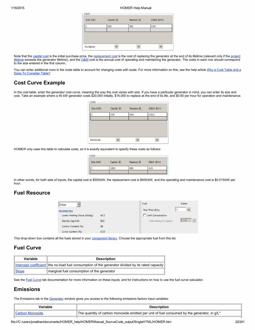
CostsThe Costs box includes the initial capital cost and replacement cost of the generator, as well as annual operation and maintenance (O&M) costs. When specifyingthe capital and replacement costs, remember to account for all costs associated with the generator, including installation.
1/16/2015 HOMER Help Manual
file:///C:/users/jonathan/documents/HOMER_help/HOMERManual_SourceCode_output/SingleHTML/HOMER.htm 22/241
Note that the capital cost is the initial purchase price, the replacement cost is the cost of replacing the generator at the end of its lifetime (relevant only if the projectlifetime exceeds the generator lifetime), and the O&M cost is the annual cost of operating and maintaining the generator. The costs in each row should correspondto the size entered in the first column.
You can enter additional rows in the costs table to account for changing costs with scale. For more information on this, see the help article Why a Cost Table and aSizes To Consider Table?
Cost Curve ExampleIn the cost table, enter the generator cost curve, meaning the way the cost varies with size. If you have a particular generator in mind, you can enter its size andcost. Take an example where a 40 kW generator costs $20,000 initially, $16,000 to replace at the end of its life, and $0.60 per hour for operation and maintenance.
HOMER only uses this table to calculate costs, so it is exactly equivalent to specify these costs as follows:
In other words, for both sets of inputs, the capital cost is $500/kW, the replacement cost is $400/kW, and the operating and maintenance cost is $0.015/kW perhour.
Fuel Resource
This dropdown box contains all the fuels stored in your component library. Choose the appropriate fuel from this list.
Fuel Curve
Variable DescriptionIntercept coefficient the noload fuel consumption of the generator divided by its rated capacity
Slope marginal fuel consumption of the generator
See the Fuel Curve tab documentation for more information on these inputs, and for instructions on how to use the fuel curve calculator.
EmissionsThe Emissions tab in the Generator window gives you access to the following emissions factors input variables:
Variable DescriptionCarbon Monoxide The quantity of carbon monoxide emitted per unit of fuel consumed by the generator, in g/L*

1/16/2015 HOMER Help Manual
file:///C:/users/jonathan/documents/HOMER_help/HOMERManual_SourceCode_output/SingleHTML/HOMER.htm 23/241
Unburned Hydrocarbons The quantity of unburned hydrocarbons emitted per unit of fuel consumed by the generator, in g/L*Particulate Matter The quantity of particulate matter emitted per unit of fuel consumed by the generator, in g/L*
Proportion of Fuel Sulfur Convertedto PM
The fraction of the sulfur in the fuel that is emitted as particulate matter (the rest is emitted as sulfurdioxide), in %
Nitrogen Oxides The quantity of nitrogen oxides emitted per unit of fuel consumed by the generator, in g/L*
*These units will be in g/m3 for fuels that are measured in m3 and g/kg for fuels measured in kg.
Note: To the right of each numerical input is a sensitivity button ( )which allows you to do a sensitivity analysis on that variable. For more information, pleasesee Why would I want to do a sensitivity analysis?
MaintenanceHOMER can include the cost and downtime for specific maintenance tasks in the simulation. Check the option "Consider Maintenance Schedule" if you wish to usethis option. The following inputs, found under the "Maintenance" tab, can be used to define a maintenance requirement:
Variable DescriptionProcedure Descriptive name for the maintenance item
Interval (op hrs.) How often the maintenance will have to be performed, in terms of number hours that the generator is operating
Down time (realhrs.)
Number of hours for which the generator will be forced off once the number when the end of the maintenance interval isreached
Cost ($) Cost of the maintenance procedure. This cost will be incurred at the end of each maintenance interval
The generator maintenance down time will only be considered in the results if the maintenance occurs within the first year of the simulation. This is because theHOMER engine extrapolates for results beyond one year. This will not affect the dispatch desicions, since the engine amortizes the cost of the maintenanceoperation over the interval and so will include the anticipated cost in dispatch at every time step.
This behavior could cause an unexpected absence of a capacity shortage resulting from generator down time. For example, consider a system with one generatorand a load, and zero capacity shortage allowed. Adding a maintenance item with an interval of 1,000 hours would make this system infeasible, since there wouldbe a capacity shortage during the down time hours. If we set the maintenance interval to 9,000 hours, however, HOMER will report that the case is feasible.
ScheduleBy default, HOMER decides each time step whether or not to operate the generator based on the electrical demand and the economics of the generator versusother power sources. You can, however, use the generator schedule inputs to prevent HOMER from using the generator during certain times, or force it to use thegenerator during other times.
The schedule diagram on the right side of the window shows the times of the day and year during which the generator must operate and must not operate, andwhen HOMER can decide based on economics. In the example below, the generator must operate between 8am and 8pm every day. At all other times, HOMERcan decide whether to run the generator based on economics.
It is also possible to treat weekdays and weekends differently. In the example below, the generator may not operate during school hours, which are 8am to 5pm onweekdays, except for July and August. (Such constraints are sometimes necessary in small village power systems because of generator noise.) At all other times,HOMER can decide whether to run the generator or not.

1/16/2015 HOMER Help Manual
file:///C:/users/jonathan/documents/HOMER_help/HOMERManual_SourceCode_output/SingleHTML/HOMER.htm 24/241
In the example below, the generator must operate during weekday evenings May through September, and must not operate before 7am or after 10pm throughoutthe year. At all other times, HOMER can decide whether to run the generator or not.
To modify the generator schedule, choose a drawing mode on the left side of the window and then draw on the schedule diagram on the right side of the window.For example, to force the generator to operate weekdays afternoons in July:
1. Click the button labeled Forced On2. Click the button labeled Weekdays3. Move the mouse to the column representing July and row representing 12pm1pm4. Click and drag the mouse to the row representing 5pm6pm
Note that when you move the mouse over the schedule diagram, the cursor changes depending on whether you have selected weekdays, weekends, or all week.
Note: To the right of each numerical input is a sensitivity button ( )which allows you to do a sensitivity analysis on that variable. For more information, pleasesee Why would I want to do a sensitivity analysis?
See also:
How HOMER calculates emissions
For more informationThe HOMER Support Site has a searchable knowledgebase and additional support options.
HOMER online contains the latest information on model updates, as well as sample files, resource data, and contact information.
© 20122014 HOMER Energy, LLCLast modified: October 29, 2004
[TOP]
2.2.1.1 Fuel Curve
Fuel Curve
The Fuel Curve tab provides assistance in calculating the two fuel curve inputs on the Generator window.
Generator sizeEnter the rated size of the generator for which you have fuel consumption data.
Fuel consumption data
In this table, you enter data points on the generator's fuel curve. You must enter at least two points, but you can enter more than that if you have sufficient data.
Note: The units of the fuel consumption column change according to the units of the fuel this generator uses. If the generator consumes a fuel denominated inliters, the units of the fuel consumption column will be L/hr. But if the fuel is denominated in cubic meters, the units of the fuel consumption will be m3/hr.
HOMER plots the fuel consumption data in the fuel curve. The example shown below corresponds to the data shown in the table above. HOMER fits a line to thedata points using the linear leastsquares method. The straight line represents the line of best fit, which in this example fits the data very well. A straight line may

1/16/2015 HOMER Help Manual
file:///C:/users/jonathan/documents/HOMER_help/HOMERManual_SourceCode_output/SingleHTML/HOMER.htm 25/241
not represent certain types of generators, such as fuel cells and variablespeed diesels, quite as well. But for the more common constantspeed internal combustiongenerators and microturbines, the straightline fuel curve is a good fit.
The yintercept of the fuel curve is sometimes called the "noload fuel consumption". This represents the amount of fuel consumed by the generator when idling(producing no electricity). The slope of the fuel curve is sometimes called the "marginal fuel consumption".
Using the straight line it fits to the fuel consumption data, HOMER calculates the generator's efficiency at various points between zero output and rated output. Thatcalculation takes into account the energy content of the fuel. HOMER plots the results as the efficiency curve.
Calculated fuel curve parametersNote that HOMER's two fuel curve inputs are not the intercept and slope, but rather the intercept coefficient and the slope. The intercept coefficient is equal to theintercept divided by the generator capacity. Defining the fuel curve in this manner allows HOMER to apply it to a family of generators, over a range of sizes. This isnecessary when you enter multiple sizes in the "Sizes to consider" table of the Generator Inputs window, since the fuel curve inputs apply to each specifiedgenerator size.
The units of the two fuel curve parameters correspond to the units of the fuel used by the generator. For example, if the fuel is measured in liters, the fuel curveslope and intercept coefficient will be in units of L/hr/kW (liters per hour per kilowatt, or equivalently L/kWh).
When you click OK, HOMER copies the two calculated parameters to the Generator Inputs window.
See also
Fuel curve intercept coefficient
Fuel curve slope
Generator Inputs window
For more informationThe HOMER Support Site has a searchable knowledgebase and additional support options.
HOMER online contains the latest information on model updates, as well as sample files, resource data, and contact information.
© 20122014 HOMER Energy, LLCLast modified: July 9, 2004
[TOP]
2.2.2 PV (Photovoltaic)
Photovoltaic Panels
The PV inputs window allows you to enter the cost, performance characteristics and orientation of an array of photovoltaic (PV) panels as well as choose the sizesyou want HOMER to consider as it searches for the optimal system. This window also provides access to the following tabs:
Inverter : If the "Electrical Bus" is set to "AC", inverter parameters are specified here.MPPT: If the "Electrical Bus" is set to "DC", the parameters of the maximum power point tracker (DC to DC converter) are set here.Advanced Inputs, where you can set certain advanced variables Temperature: specify whether to consider the effect of ambient temperature on panel efficiency, and if so set the relevant inputs
You can also access the Solar Resource window by clicking the button at the top of the screen.
Costs
1/16/2015 HOMER Help Manual
file:///C:/users/jonathan/documents/HOMER_help/HOMERManual_SourceCode_output/SingleHTML/HOMER.htm 26/241
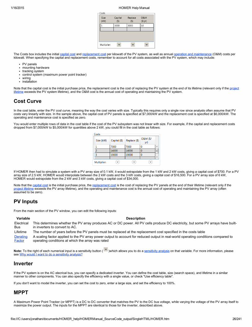
The Costs box includes the initial capital cost and replacement cost per kilowatt of the PV system, as well as annual operation and maintenance (O&M) costs perkilowatt. When specifying the capital and replacement costs, remember to account for all costs associated with the PV system, which may include:
PV panelsmounting hardwaretracking systemcontrol system (maximum power point tracker)wiringinstallation
Note that the capital cost is the initial purchase price, the replacement cost is the cost of replacing the PV system at the end of its lifetime (relevant only if the projectlifetime exceeds the PV system lifetime), and the O&M cost is the annual cost of operating and maintaining the PV system.
Cost CurveIn the cost table, enter the PV cost curve, meaning the way the cost varies with size. Typically this requires only a single row since analysts often assume that PVcosts vary linearly with size. In the sample above, the capital cost of PV panels is specified at $7,000/kW and the replacement cost is specified at $6,000/kW. Theoperating and maintenance cost is specified as zero.
You would enter multiple rows of data in the cost table if the cost of the PV subsystem was not linear with size. For example, if the capital and replacement costsdropped from $7,000/kW to $5,000/kW for quantities above 2 kW, you could fill in the cost table as follows:
If HOMER then had to simulate a system with a PV array size of 0.1 kW, it would extrapolate from the 1 kW and 2 kW costs, giving a capital cost of $700. For a PVarray size of 2.5 kW, HOMER would interpolate between the 2 kW costs and the 3 kW costs, giving a capital cost of $16,500. For a PV array size of 6 kW,HOMER would extrapolate from the 2 kW and 3 kW costs, giving a capital cost of $34,000.
Note that the capital cost is the initial purchase price, the replacement cost is the cost of replacing the PV panels at the end of their lifetime (relevant only if theproject lifetime exceeds the PV array lifetime), and the operating and maintenance cost is the annual cost of operating and maintaining the PV array (oftenassumed to be zero).
PV InputsFrom the main section of the PV window, you can edit the following inputs:
Variable DescriptionElectricalBus
This determines whether the PV array produces AC or DC power. All PV cells produce DC electricity, but some PV arrays have builtin inverters to convert to AC.
Lifetime The number of years before the PV panels must be replaced at the replacement cost specified in the costs tableDeratingFactor
A scaling factor applied to the PV array power output to account for reduced output in realworld operating conditions compared tooperating conditions at which the array was rated
Note: To the right of each numerical input is a sensitivity button ( )which allows you to do a sensitivity analysis on that variable. For more information, pleasesee Why would I want to do a sensitivity analysis?
InverterIf the PV system is on the AC elecrical bus, you can specify a dedicated inverter. You can define the cost table, size (search space), and lifetime in a similarmanner to other components. You can also specify the efficiency with a single value, or check "Use efficiency table".
If you don't want to model the inverter, you can set the cost to zero, enter a large size, and set the efficiency to 100%.
MPPTA Maximum Power Point Tracker (or MPPT) is a DC to DC converter that matches the PV to the DC bus voltage, while varying the voltage of the PV array itself tomaximize the power output. The inputs for the MPPT are identical to those for the inverter, described above.

1/16/2015 HOMER Help Manual
file:///C:/users/jonathan/documents/HOMER_help/HOMERManual_SourceCode_output/SingleHTML/HOMER.htm 27/241
Advanced InputsThe Advanced Input tab contains options that affect the calculation of the PV power output. The article How HOMER Calculates the Radiation Incident on the PVcontains more information on ground reflectance, panel slope, and panel azimuth.
Variable Description Ground Reflectance The fraction of solar radiation incident on the ground that is reflected, in %Tracking System The type of tracking system used to direct the PV panels towards the sunPanel Slope The angle at which the panels are mounted relative to the horizontal, in degreesPanel Azimuth The direction towards which the panels face, in degrees
TemperatureThe Temperature tab contains setting model or ignore temperature effects. See How HOMER Calculates the PV Array Output for detailed information ontemperature effects on power, nominal operating cell temperature, and efficiency at standard test conditions.
Variable DescriptionConsider Effect of Temperature HOMER will consider the effect of PV cell temperature on the power output of the PV array
Temperature Coefficient of Power A number indicating how strongly the power output of the PV array depends on cell temperature, in%/degrees Celsius
Nominal Operating CellTemperature The cell temperature at 0.8 kW/m2, 20°C ambient temperature, and 1 m/s wind speed, in degrees Celsius
Efficiency at Standard TestConditions The maximum power point efficiency under standard test conditions, in %
See also:
How HOMER calculates the radiation incident on the PV array
How HOMER calculates the PV cell temperature
How HOMER calculates the output of the PV array
Search Space window
Standard test conditions
For more informationThe HOMER Support Site has a searchable knowledgebase and additional support options.
HOMER online contains the latest information on model updates, as well as sample files, resource data, and contact information.
© 20122014 HOMER Energy, LLCLast modified: July 2, 2013
[TOP]
2.2.3 Wind Turbine
Wind Turbine
The Wind Turbine inputs window allows you to choose the type of wind turbine you want to model, specify its costs, and tell HOMER how many to consider as itsearches for the optimal system. This window also provides access to the following tabs:
Power Curve: view and edit the power curve for the selected wind turbineTurbine Losses: specify different loss modesMaintenance: consider maintenance tasks, costs, and down time
You can access the Wind Resource window by clicking the button at the top of the screen.
Turbine type
This dropdown menu located at the top of the wind turbine set up page contains all the wind turbine types stored in your component library . Choose anappropriate wind turbine model from this list. When you make a selection with this dropdown box, a summary of the selected wind turbine's properties are

1/16/2015 HOMER Help Manual
file:///C:/users/jonathan/documents/HOMER_help/HOMERManual_SourceCode_output/SingleHTML/HOMER.htm 28/241
displayed in the space below. Click on "Add Wind Turbine" to add the selected turbine to your model.
Costs
In the Costs table, the capital cost is the initial purchase price for a turbine, the replacement cost is the cost of replacing the wind turbine at the end of its lifetime(relevant only if the project lifetime exceeds the wind turbine lifetime), and the operating and maintenance cost is the annual cost of operating and maintaining theturbine (about 2% percent of the capital cost is typical).
When specifying the capital and replacement costs, remember to account for all costs associated with the wind energy system, which may include:
turbine rotor and towercontrol system wiringinstallation
Cost CurveIn the cost table, enter the wind turbine's cost curve in as much detail as you would like. In the simplest case, where each wind turbine costs the same regardless ofhow many you purchase, you only need to enter one row of data in the cost table. You would enter a quantity of one, along with the perturbine capital,replacement, and operating and maintenance costs. HOMER extrapolates these costs as needed, so if you modeled a system with three wind turbines, theassociated capital, replacement, and O&M costs would be three times the values entered in the cost table.
You would enter multiple rows of data in the cost table if the cost of wind power was not directly proportional to the number of wind turbines purchased. In theexample shown above, the second wind turbine is cheaper than the first (this could be because of a volume discount from the manufacturer or because certainfixed costs can be spread over multiple turbines). If the third turbine were cheaper yet, another row of costs could be added. With just these two rows specifiedthough, HOMER would extrapolate the costs by assuming that the third, fourth, and subsequent turbines cost the same as the second.
Search SpaceEnter the quantity of turbines you would like, or enter several quantities for HOMER to consider in the system optimization. Include a zero if you would like HOMERto consider systems without this wind turbine.
Electrical BusSelect whether the turbine will produce AC or DC power. Power electronics are not modeled explicitly, but you can account for a dedicated converter efficiency byscaling the power curve.
Site Specific Inputs
Variable DescriptionLifetime The number of years the turbine is expected to last before it requires replacement
Hub height The height above ground of the hub (the center of the rotor), in meters
Consider ambient temperatureeffects?
HOMER will compensate for the change in air density with temperature. If checked, you must define atemperature resource.
Note: To the right of each numerical input is a sensitivity button ( )which allows you to do a sensitivity analysis on that variable. For more information, pleasesee Why would I want to do a sensitivity analysis?
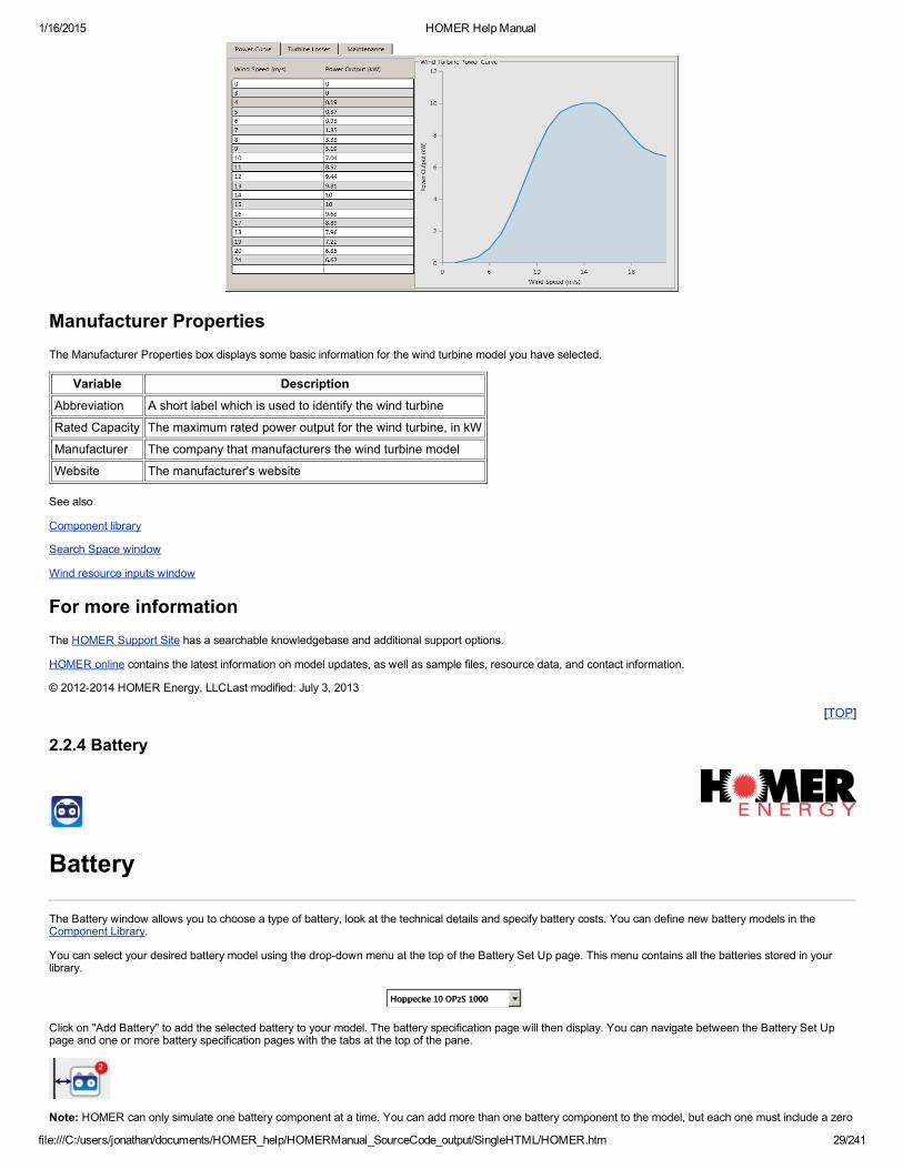
Power CurveThe Power Curve tab in the Wind Turbine window allows you to view the power curve of the selected wind turbine model in both tabular and graphical form. Awind turbine's power curve shows how much power it will produce depending on the incoming hubheight wind speed at standard atmospheric conditions. Use thisgraph to verify that the wind turbine you have selected is an appropriate size for your system.
1/16/2015 HOMER Help Manual
file:///C:/users/jonathan/documents/HOMER_help/HOMERManual_SourceCode_output/SingleHTML/HOMER.htm 29/241
Manufacturer PropertiesThe Manufacturer Properties box displays some basic information for the wind turbine model you have selected.
Variable DescriptionAbbreviation A short label which is used to identify the wind turbine
Rated Capacity The maximum rated power output for the wind turbine, in kW
Manufacturer The company that manufacturers the wind turbine model
Website The manufacturer's website
See also
Component library
Search Space window
Wind resource inputs window
For more informationThe HOMER Support Site has a searchable knowledgebase and additional support options.
HOMER online contains the latest information on model updates, as well as sample files, resource data, and contact information.
© 20122014 HOMER Energy, LLCLast modified: July 3, 2013
[TOP]
2.2.4 Battery
Battery
The Battery window allows you to choose a type of battery, look at the technical details and specify battery costs. You can define new battery models in theComponent Library.
You can select your desired battery model using the dropdown menu at the top of the Battery Set Up page. This menu contains all the batteries stored in yourlibrary.
Click on "Add Battery" to add the selected battery to your model. The battery specification page will then display. You can navigate between the Battery Set Uppage and one or more battery specification pages with the tabs at the top of the pane.
Note: HOMER can only simulate one battery component at a time. You can add more than one battery component to the model, but each one must include a zero

1/16/2015 HOMER Help Manual
file:///C:/users/jonathan/documents/HOMER_help/HOMERManual_SourceCode_output/SingleHTML/HOMER.htm 30/241
in the search space. HOMER will simulate each of the battery types, one component at a time.
Costs
The Costs box includes the initial capital cost and replacement cost per battery, as well as annual operation and maintenance (O&M) costs per battery. Whenspecifying the capital and replacement costs, remember to account for all costs associated with the battery, including installation.
Note that the capital cost is the initial purchase price, the replacement cost is the cost of replacing the battery at the end of its lifetime (relevant only if the projectlifetime exceeds the battery lifetime), and the O&M cost is the annual cost of operating and maintaining the battery.
Note: Below each numerical input is a sensitivity button ( )which allows you to do a sensitivity analysis on that variable. For more information, please see Whywould I want to do a sensitivity analysis?
Cost CurveIn this table, enter the battery's cost curve in as much detail as you would like. In the simplest case, where each battery costs the same regardless of how manyyou puchase, you only need to enter one row of data in the cost table. You would enter a quantity of one, along with the perbattery capital, replacement, andoperating and maintenance costs. In the example shown above, each battery costs $1,800 initially, $1,600 to replace, and $10 annually for operating andmaintenance. HOMER extrapolates these costs as needed, so if you modeled a system with three batteries, the associated capital, replacement, and O&M costswould be three times the values entered in the cost table.
You would enter multiple rows of data in the cost table if the battery bank's costs were not directly proportional to the number of batteries purchased. In theexample shown below, the fixed cost of the battery bank is $2,000 initially plus $30/yr for operating and maintenance. (This could be the cost of a room or a buildingin which to house the batteries.) Each battery then costs $700 plus $5/yr for operating and maintenance.
Note: HOMER will not assess this $2,000 capital cost to a system that contains zero batteries. It applies only to systems containing battery banks. To add a fixedcapital or O&M cost, see Economics Inputs.
Note that the capital cost is the initial purchase price, the replacement cost is the cost of replacing the batteries at the end of their lifetime (relevant only if the projectlifetime exceeds the battery lifetime, which is a calculated output), and the O&M cost is the annual cost of operating and maintaining the battery bank.
HOMER will use the number of batteries/strings you entered in the cost table to calculate the corresponding costs, interpolating and extrapolating as necessary .You can see the results in the cost curve graph.
Search Space with Strings
Two or more batteries connected in series form a string, and strings are connected in parallel to form a battery bank. Batteries per string determines whether thesizes to consider table shows numbers of batteries or numbers of strings. In results tables and graphs, HOMER always displays the number of batteries, regardlessof how you specify the number of batteries in the sizes to consider table. When the number of batteries per string is
one, the sizes to consider table shows numbers of batteries;two or more, the sizes to consider table shows numbers of strings.
HOMER shows the DC bus voltage in parentheses next to the number of batteries per string. (The bus voltage is the battery's nominal voltage multiplied by thenumber of batteries per string.) You can use that to decide how many batteries to use per string.
Note: If you want to determine the optimal storage capacity and you are not concerned with the system voltage, you can set the number of batteries per string toone and ignore the bus voltage. This approach might be appropriate for a preliminary sizing analysis.
Battery Inputs

1/16/2015 HOMER Help Manual
file:///C:/users/jonathan/documents/HOMER_help/HOMERManual_SourceCode_output/SingleHTML/HOMER.htm 31/241
Variable Description
Batteries per String A string is a set of batteries connected in series. The number of batteries per string multiplied by the nominal voltageis the bus voltage.
Initial State of Charge The state of charge of the battery bank at the beginning of the HOMER simulation, in %
Minimum State ofCharge A lower limit on the state of charge of the battery bank, in %
Enforce Minimum BatteryLife Enable the Minimum Battery Life constraint
Minimum Battery Life A lower limit on the lifetime of the battery bank (systems that do not meet this constraint are discarded as infeasible)
Note: To the right of each numerical input is a sensitivity button ( )which allows you to do a sensitivity analysis on that variable. For more information, pleasesee Why would I want to do a sensitivity analysis?
Minimum Battery LifeThe minimum battery life is a lower limit on the lifetime of the battery bank. This contraint is not normally necessary, but you can use it if necessary to preventHOMER from recommending a relatively small battery bank that lasts an unacceptably short time. For example, HOMER may determine that the optimal systemcontains a small battery bank that lasts only 1.5 years before needing replacement. If that 1.5 year replacement cycle is unacceptably short, you could implement aminimum 4 year battery lifetime, which would cause HOMER to discard that optimal system and choose another, probably with a larger battery bank. It would be amore expensive system (otherwise it would have been optimal without the battery life constraint) but it would conform to the constraint.
Manufacturer PropertiesThe Manufacturer Properties box displays some basic information for the battery type you have selected.
Variable DescriptionManufacturer The company that manufacturers the battery model
Website Web address where more information on the battery model can be found
Nominal Voltage The rated voltage (it is called nominal because the actual voltage varies according to the battery's operating conditions andstate of charge)
Nominal Capacity The amount of energy that can be drawn out of the battery at the rated discharge current, starting from a fully charged state,in kWh
LifetimeThroughput The total amount of energy that can be cycled through the battery before it needs replacement, in kWh
Abbreviation The abbreviation used in HOMER
Note: HOMER does not model the battery charge controller as a separate component. You must include its cost and efficiency in the values you specify for thebattery or in other components in the system.
See also
How can I specify the DC bus voltage?
Component Library Battery
For more informationThe HOMER Support Site has a searchable knowledgebase and additional support options.
HOMER online contains the latest information on model updates, as well as sample files, resource data, and contact information.
© 20122014 HOMER Energy, LLCLast modified: July 2, 2013
[TOP]
2.2.5 Flywheel
Flywheel
A flywheel provides operating reserve on the AC bus, helping to absorb sudden increases in renewable power output or to make up for sudden decreases inrenewable power output. rapid surges of power from renewable power from the wind turbine (or photovoltaic array) or alternatively supplying power to make up for

1/16/2015 HOMER Help Manual
file:///C:/users/jonathan/documents/HOMER_help/HOMERManual_SourceCode_output/SingleHTML/HOMER.htm 32/241
short term lulls.
A flywheel can also maintain power quality and system stability through active and reactive power control, although HOMER does not explicitly model those effects.These effects can be important in medium and high renewable penetration systems serving isolated networks or on soft grids (such as near the end of distributionlines).
Flywheels typically connect to the AC bus via an AC/AC inverter system that converts the variablefrequency AC power from the flywheel rotor to constantfrequency, gridquality AC power on the AC bus.
Use the Flywheel Inputs window to choose the type of flywheel you want to model, specify its costs, and tell HOMER how many to consider as it searches for theoptimal system configuration.
Flywheel typeThis dropdown box contains all the flywheel types stored in your component library. Choose an appropriate flywheel model from this list. When you make aselection with this dropdown box, a summary of the selected flywheel's properties appears in the space below. To add a new flywheel or edit the properties, usethe component library.
CostsIn the cost table, enter the flywheel's cost curve in as much detail as you would like. In the simplest case, where each flywheel costs the same regardless of howmany you purchase, you only need to enter one row of data in the cost table. You would enter a quantity of one, along with the perflywheel capital, replacement,and operating and maintenance costs. HOMER extrapolates these costs as needed, so if you modeled a system with three flywheels, the associated capital,replacement, and O&M costs would be three times the values you entered in the cost table.
You would enter multiple rows of data in the cost table if the cost of flywheels was not directly proportional to the number of flywheels purchased. For example, thesecond flywheel may cost less than the first due to a volume discount or because certain fixed costs can be spread over multiple flywheels. If the third flywheelwere cheaper yet, you could add a third row of costs.
Note that the capital cost is the initial purchase price, the replacement cost is the cost of replacing the flywheel at the end of its lifetime (relevant only if the projectlifetime exceeds the flywheel lifetime), and the operating and maintenance cost is the annual cost of operating and maintaining the flywheel.
Search SpaceIn this table, enter the number of flywheels you want HOMER to consider as it searches for the optimal system configuration. Be sure to include a zero if you wanttoconsider systems without flywheels. HOMER will use the information you entered in the cost table to calculate the corresponding costs, interpolating andextrapolating as necessary. You can see the results in the cost curve graph.
Note: You can also access the values in this table using the Search Space window.
Properties
Variable Description
Lifetime The number of years you expect the flywheel to last before it requires replacement
Note: To the right of each numerical input is a sensitivity button ( )which allows you to do a sensitivity analysis on that variable. For more information, pleasesee Why would I want to do a sensitivity analysis?
See also
Operating reserve
Component library
Search Space window
For more informationThe HOMER Support Site has a searchable knowledgebase and additional support options.
HOMER online contains the latest information on model updates, as well as sample files, resource data, and contact information.
© 20122014 HOMER Energy, LLCLast modified: October 21, 2009
[TOP]
2.2.6 Converter
Converter
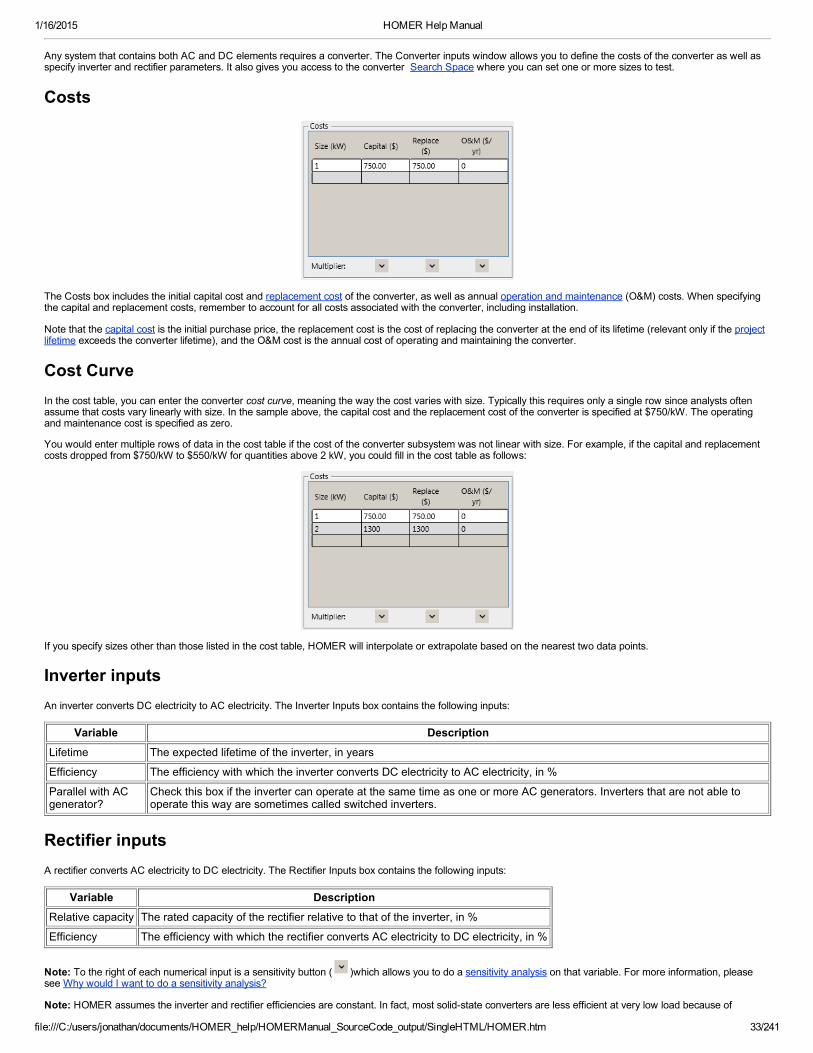
1/16/2015 HOMER Help Manual
file:///C:/users/jonathan/documents/HOMER_help/HOMERManual_SourceCode_output/SingleHTML/HOMER.htm 33/241
Any system that contains both AC and DC elements requires a converter. The Converter inputs window allows you to define the costs of the converter as well asspecify inverter and rectifier parameters. It also gives you access to the converter Search Space where you can set one or more sizes to test.
Costs
The Costs box includes the initial capital cost and replacement cost of the converter, as well as annual operation and maintenance (O&M) costs. When specifyingthe capital and replacement costs, remember to account for all costs associated with the converter, including installation.
Note that the capital cost is the initial purchase price, the replacement cost is the cost of replacing the converter at the end of its lifetime (relevant only if the projectlifetime exceeds the converter lifetime), and the O&M cost is the annual cost of operating and maintaining the converter.
Cost CurveIn the cost table, you can enter the converter cost curve, meaning the way the cost varies with size. Typically this requires only a single row since analysts oftenassume that costs vary linearly with size. In the sample above, the capital cost and the replacement cost of the converter is specified at $750/kW. The operatingand maintenance cost is specified as zero.
You would enter multiple rows of data in the cost table if the cost of the converter subsystem was not linear with size. For example, if the capital and replacementcosts dropped from $750/kW to $550/kW for quantities above 2 kW, you could fill in the cost table as follows:
If you specify sizes other than those listed in the cost table, HOMER will interpolate or extrapolate based on the nearest two data points.
Inverter inputsAn inverter converts DC electricity to AC electricity. The Inverter Inputs box contains the following inputs:
Variable DescriptionLifetime The expected lifetime of the inverter, in years
Efficiency The efficiency with which the inverter converts DC electricity to AC electricity, in %
Parallel with ACgenerator?
Check this box if the inverter can operate at the same time as one or more AC generators. Inverters that are not able tooperate this way are sometimes called switched inverters.
Rectifier inputsA rectifier converts AC electricity to DC electricity. The Rectifier Inputs box contains the following inputs:
Variable DescriptionRelative capacity The rated capacity of the rectifier relative to that of the inverter, in %
Efficiency The efficiency with which the rectifier converts AC electricity to DC electricity, in %
Note: To the right of each numerical input is a sensitivity button ( )which allows you to do a sensitivity analysis on that variable. For more information, pleasesee Why would I want to do a sensitivity analysis?
Note: HOMER assumes the inverter and rectifier efficiencies are constant. In fact, most solidstate converters are less efficient at very low load because of

1/16/2015 HOMER Help Manual
file:///C:/users/jonathan/documents/HOMER_help/HOMERManual_SourceCode_output/SingleHTML/HOMER.htm 34/241
standing losses.
For more informationThe HOMER Support Site has a searchable knowledgebase and additional support options.
HOMER online contains the latest information on model updates, as well as sample files, resource data, and contact information.
© 20122014 HOMER Energy, LLCLast modified: October 29, 2004
[TOP]
2.2.7 Boiler
Boiler
This feature requires the Combined Heat and Power Module.
Click for more information.
HOMER considers the serving of thermal load to be less important than the serving of electric load. When dispatching generators to serve the electric load,HOMER considers the value of any usable waste heat that can be recovered from each generator, but it will not dispatch a generator simply to serve the thermalload. It assumes the boiler can serve any thermal load that the generators do not. In other words, HOMER treats the boiler as a backup source of heat that canserve any amount of thermal load whenever necessary. HOMER automatically adds a boiler to the system when you add a thermal load. There is no costassociated with the boiler.
Fuel ResourceThis dropdown box contains all the fuels stored in your component library. Choose the appropriate fuel from this list. When a fuel is selected from the dropdownmenu, detailed properties of the selected fuel are displayed.
You can create a new fuel type and remove or redefine an existing fuel in the library.
Fuel Price
Enter the price for the chosen fuel, and add sensitivity values for this cost. Will depend on the fuel, either in $/L or $/m3.
EfficiencyEnter the fraction of the fuel's energy that gets converted to heat in the boiler.
Emissions factorsIn this box, you can modify the following variables:
Variable DescriptionCarbon Monoxide Emissions Factor The quantity of carbon monoxide (in grams) emitted per unit of fuel consumed by the boiler
Unburned Hydrocarbons EmissionsFactor The quantity of unburned hydrocarbons (in grams) emitted per unit of fuel consumed by the boiler
Particulate Matter Emissions Factor The quantity of particulate matter (in grams) emitted per unit of fuel consumed by the boiler
Proportion of fuel sulfur emitted as PM The fraction of the sulfur in the fuel that is emitted as particulate matter (the rest is emitted as sulfurdioxide)
Nitrogen Oxides Emissions Factor The quantity of nitrogen oxides (in grams) emitted per unit of fuel consumed by the boiler

1/16/2015 HOMER Help Manual
file:///C:/users/jonathan/documents/HOMER_help/HOMERManual_SourceCode_output/SingleHTML/HOMER.htm 35/241
See also:
How HOMER calculates emissions
For more informationThe HOMER Support Site has a searchable knowledgebase and additional support options.
HOMER online contains the latest information on model updates, as well as sample files, resource data, and contact information.
© 20122014 HOMER Energy, LLCLast modified: October 29, 2004
[TOP]
2.2.8 Hydro
Hydro
This feature requires the Hydro Module.
Click for more information.
HOMER can only consider a single size of hydro system. For this reason, the Hydro Inputs window does not contain tables of costs or sizes to consider. Instead,you simply specify the cost and properties of the size of hydro system that you want to consider.
EconomicsThese inputs specify the costs of the hydro system. Remember to include all costs associated with the hydro system, including the civil works.
Variable DescriptionCapital Cost The initial capital cost of the hydro system
Replacement Cost The replacement cost of the hydro system
O&M Cost The annual cost of operating and maintaining the hydro system
Lifetime The number of years that the hydro system is expected to last
TurbineThese inputs specify the properties of the hydro turbine.
Variable DescriptionAvailableHead The vertical drop between the intake and the turbine
DesignFlow Rate
The flow rate for which this hydro turbine was designed. It is often the flow rate at which the turbine operates at maximumefficiency.
MinimumFlow Ratio
The minimum flow rate of the hydro turbine, as a percentage of its design flow rate. Below this rate, the turbine will produce nopower.
MaximumFlow Ratio
The maximum flow rate of the hydro turbine, as a percentage of its design flow rate. The turbine will generate power at thespecified efficiency up to this flow. Additional flow above this level will not increase turbine power output.
Efficiency The efficiency with which the hydro system converts the energy in the water to electricity
GeneratorType The type of current (AC or DC) produced by the hydro turbine
Intake pipeThis input allows you to specify the frictional losses that occur in the intake pipe which reduce the energy of the water before it goes through the hydro turbine.
Variable DescriptionPipe Head Loss Pipe friction losses expressed as a percentage of the available head
Tip: For assistance in calculating the pipe head loss, click the Pipe Head Loss Calculator button.

1/16/2015 HOMER Help Manual
file:///C:/users/jonathan/documents/HOMER_help/HOMERManual_SourceCode_output/SingleHTML/HOMER.htm 36/241
Systems to considerThe choice you make in this section will affect which systems HOMER considers as it searches for the leastcost system.
Variable DescriptionSimulate systems both with andwithout the hydro turbine
Choose this option to simulate systems both with and without the hydro turbine. HOMER will rank the systemsaccording to cost so you can see whether or not the hydro system is costeffective.
Include the hydro turbine in allsimulated systems Choose this option if you want all systems to include the hydro turbine.
Note: To the right of each numerical input is a sensitivity button ( )which allows you to do a sensitivity analysis on that variable. For more information, pleasesee Why would I want to do a sensitivity analysis?
See also:
Calculating hydro power output
Pipe Head Loss Calculator window
The hydro section of Recommended Reading
Why do I have to scale load and resource data?
For more informationThe HOMER Support Site has a searchable knowledgebase and additional support options.
HOMER online contains the latest information on model updates, as well as sample files, resource data, and contact information.
© 20122014 HOMER Energy, LLCLast modified: December 27, 2007
[TOP]
2.2.8.1 Pipe Head Loss Calculator
Pipe Head Loss Calculator
This window helps you calculate the head loss in the intake pipe of the hydro power system. Enter the flow rate along with the length, diameter, and material of thepipe, and HOMER will calculate the resulting head loss using the standard fluid mechanics equations on which the Moody diagram is based.
This window provides assistance in estimating the value of the pipe head loss.
AvailableHead The vertical drop between the intake and the turbine (specified on the Hydro input window)
Design FlowRate
The flow rate for which you wish to calculate the head loss. Although in reality the head loss changes with flow rate, HOMERassumes the head loss is constant.
Pipe Length The length of the pipe between the intake and the turbine
PipeDiameter
The diameter of a circular pipe. If the pipe is not circular, you must calculate and specify the hydraulic diameter. An explanation ofhydraulic diameter is available in most standard fluid mechanics textbooks.
PipeMaterial This affects the pipe loss because each material has a particular roughness
AbsoluteHead Loss
The result of the DarcyWeisbach equation of fluid mechanics. More information on the DarcyWeisbach equation is available inmost standard fluid mechanics textbooks.
RelativeHead Loss The absolute head loss divided by the available head. This value gets copied into the Hydro input window when you click OK.
When you click OK, HOMER will copy the calculated value into the pipe head loss input box on the Hydro Inputs window.
If you enter a flow rate so high as to be impossible through the pipe as specified, HOMER will display a warning message.
For more informationThe HOMER Support Site has a searchable knowledgebase and additional support options.
HOMER online contains the latest information on model updates, as well as sample files, resource data, and contact information.

1/16/2015 HOMER Help Manual
file:///C:/users/jonathan/documents/HOMER_help/HOMERManual_SourceCode_output/SingleHTML/HOMER.htm 37/241
© 20122014 HOMER Energy, LLCLast modified: June 21, 2004
[TOP]
2.2.9 Hydrokinetic
Hydrokinetic
The hydrokinetic component can represent several different types of lowhead hydro power generation including runoftheriver, tidal, and wave energy electricgeneration. The component is described as a turbine, but the hydrokinetic component can also represent other technologies such as a wave energy converter. Witha hydrokinetic component, you must also specify the hydrokinetic resource
The Hydrokinetic inputs window allows you to choose the type of hydrokinetic installation you want to model, specify its costs, and tell HOMER how many toconsider as it searches for the optimal system. You can also view and modify the power curve of the hydrokinetic turbine in the lower portion of the menu.
Turbine type
This dropdown menu located at the top of the hydrokinetic set up page contains all the hydrokinetic component types stored in your component library. Choose anappropriate model from this list. When you make a selection with this dropdown box, the selected turbine's properties are displayed in the space below.
Costs
In the Costs table, the capital cost is the initial purchase price for a turbine, the replacement cost is the cost of replacing the turbine at the end of its lifetime(relevant only if the project lifetime exceeds the turbine lifetime), and the operating and maintenance cost is the annual cost of operating and maintaining theturbine.
Cost CurveIn the cost table, enter the turbine's cost curve in as much detail as you would like. In the simplest case, where each turbine costs the same regardless of howmany you purchase, you only need to enter one row of data in the cost table. You would enter a quantity of one, along with the perturbine capital, replacement,and operating and maintenance costs. HOMER extrapolates these costs as needed, so if you were to model a system with three turbines, the associated capital,replacement, and O&M costs would be three times the values entered in the cost table.
You would enter multiple rows of data in the cost table if the cost of power was not directly proportional to the number of turbines purchased. In the example shownabove, the second turbine is cheaper than the first (this could be because of a volume discount from the manufacturer or because certain fixed costs can be spreadover multiple turbines). If the third turbine were cheaper yet, another row of costs could be added. With just these two rows specified though, HOMER wouldextrapolate the costs by assuming that the third, fourth, and subsequent turbines cost the same as the second.
Search SpaceEnter the quantity of turbines you would like, or enter several quantities for HOMER to consider in the system optimization. Include a zero if you would like HOMERto consider systems without this hydrokinetic turbine.
Electrical BusSelect whether the turbine will produce AC or DC power. Power electronics are not modeled explicitly, but you can account for a dedicated converter efficiency byscaling the power curve.

1/16/2015 HOMER Help Manual
file:///C:/users/jonathan/documents/HOMER_help/HOMERManual_SourceCode_output/SingleHTML/HOMER.htm 38/241
Site Specific Inputs
Variable DescriptionLifetime The number of years the turbine is expected to last before it requires replacement
Hub height The height above ground of the hub (the center of the rotor), in meters
Consider ambient temperatureeffects?
HOMER will compensate for the change in air density with temperature. If checked, you must define atemperature resource.
Note: To the right of each numerical input is a sensitivity button ( )which allows you to do a sensitivity analysis on that variable. For more information, pleasesee Why would I want to do a sensitivity analysis?
Power CurveThe Power Curve pane allows you to view the power curve of the selected turbine model in both tabular and graphical form. A turbine's power curve shows howmuch power it will produce depending on the water speed. Use this graph to verify that the turbine you have selected is an appropriate size for your system.
Manufacturer PropertiesThe Manufacturer Properties box displays some basic information for the turbine model you have selected.
Variable DescriptionAbbreviation A short label which is used to identify the turbine
Rated Capacity The maximum rated power output for the turbine, in kW
Manufacturer The company that manufacturers the turbine model
Website The manufacturer's website
See also
Component library
Search Space window
Hydrokinetic resource inputs window
For more informationThe HOMER Support Site has a searchable knowledgebase and additional support options.
HOMER online contains the latest information on model updates, as well as sample files, resource data, and contact information.
© 20122014 HOMER Energy, LLCLast modified: July 3, 2013
[TOP]
2.2.10 Thermal Load Controller

1/16/2015 HOMER Help Manual
file:///C:/users/jonathan/documents/HOMER_help/HOMERManual_SourceCode_output/SingleHTML/HOMER.htm 39/241
Thermal Load Controller
This feature requires the Combined Heat and Power Module.
Click for more information.
The thermal load controller allows excess electrical production to serve loads on the thermal bus. A thermal load controller is not required for systems with athermal load, but without it excess electrical production is not used.
SizeUse the box labeled Size to input what capacities you would like to consider.
In this table, enter the capacities you want HOMER to consider as it searches for the optimal system. HOMER will use the information you entered in the cost tableto calculate the costs of each size, interpolating and extrapolating as necessary. You can see the results in the cost curve graph.
CostsThe Costs box includes the initial capital cost and replacement cost, as well as annual operation and maintenance (O&M) costs. The table also includes the size(kW) corresponding to the costs in each row. When specifying the capital and replacement costs, remember to account for all costs associated with the thermalload controller, including installation.
Note that the capital cost is the initial purchase price, the replacement cost is the cost of replacing the thermal load controller at the end of its lifetime (relevant onlyif the project lifetime exceeds the component lifetime), and the O&M cost is the annual cost of operating and maintaining the thermal load controller.
You can enter additional rows in the costs table to account for changing costs with scale. For more information on this, see the help article Why a Cost Table and aSizes To Consider Table?
Other Inputs
Variable DescriptionLifetime The service life in years of the thermal load controller
Bus Connection Specify "AC", "DC", or "Both" for the buses from which excess electical producation can be drawn
Do not inlcude the thermal load controllerin the optimization
This option models the thermal load controller with infinite capacity. Capital, replacement, and O&Mcosts are still included in the simulation.
Note: To the right of each numerical input is a sensitivity button ( )which allows you to do a sensitivity analysis on that variable. For more information, pleasesee Why would I want to do a sensitivity analysis?
See also:
Boiler
Thermal Load
For more informationThe HOMER Support Site has a searchable knowledgebase and additional support options.
HOMER online contains the latest information on model updates, as well as sample files, resource data, and contact information.
© 20122014 HOMER Energy, LLCLast modified: October 29, 2004
[TOP]
2.2.11 Grid
1/16/2015 HOMER Help Manual
file:///C:/users/jonathan/documents/HOMER_help/HOMERManual_SourceCode_output/SingleHTML/HOMER.htm 40/241
Grid
You can add the grid like any component and it will be treated as another part of your hybrid system. If you want an offgrid system, do not add a grid component.
Grid PricesThe Grid inputs window allows you to specify the grid several different ways:
Simple rates mode allows you to specify a constant power price, sellback price, and sale capacity. All other modes require the Advanced Grid module.Real time rates define prices on an hourly basis by importing a properly formatted text file with time series data (requires Advanced Grid module).Scheduled rates permit different prices at each time of day and month of the year (requires Advanced Grid module).Grid extension mode will compare the cost of a grid extension with the cost of each standalone system configuration in the model (requires Advanced Gridmodule).
EmissionsThe Emissions tab allows you to specify emissions factors for several pollutants.
Variable DescriptionCarbon Dioxide The amount of carbon dioxide released per kWh of grid power consumed by the system, in grams/kWh
Carbon Monoxide The amount of carbon monoxide released per kWh of grid power consumed by the system, in grams/kWh
Unburned Hydrocarbons The amount of unburned hydrocarbons released per kWh of grid power consumed by the system, in grams/kWh
Particulate Matter The amount of particulate matter released per kWh of grid power consumed by the system, in grams/kWh
Sulfur Dioxide The amount of sulfur dioxide released per kWh of grid power consumed by the system, in grams/kWh
Nitrogen Oxides The amount of nitrogen oxides released per kWh of grid power consumed by the system, in grams/kWh
HOMER uses these emissions factors to calculate:
the emissions of each pollutant resulting from grid power purchasesthe avoided emissions of each pollutant resulting from grid power sales
The values of these coefficients depend on the generation mix of the electricity in your area. In an area where the majority of the electricity is produced from coal,these values will be relatively high because burning coal results in large emissions of pollutants. Natural gas generation results in somewhat lower emissions, andnuclear and hydro generation result in virtually no emissions of these pollutants.
This help file contains a table of US grid emissions factors. For additional resources, see the article on Finding data to run HOMER.
See also:
How HOMER calculates emissions
For more informationThe HOMER Support Site has a searchable knowledgebase and additional support options.
HOMER online contains the latest information on model updates, as well as sample files, resource data, and contact information.
© 20122014 HOMER Energy, LLCLast modified: October 29, 2004
[TOP]
2.2.11.1 Simple rates
Simple Rates
Simple rates mode allows you to set a constant power price and sellback price. You can also set a sale capacity, use net metering, and set emissions factors

1/16/2015 HOMER Help Manual
file:///C:/users/jonathan/documents/HOMER_help/HOMERManual_SourceCode_output/SingleHTML/HOMER.htm 41/241
associated with grid electricity. Simple rates mode is the only option that does not require the Advanced Grid module.
RatesGrid rates refer to the prices associated with buying electricity from the grid and selling electricity to the grid. In HOMER, grid rates encompass the followingvariables:
Variable DescriptionGrid Power Price($/kWh) The cost of buying power from the grid, in $/kWh.
Grid SellbackPrice ($/kWh)
The price that the utility pays you for power you sell to the grid under net metering, in $/kWh. This variable is only used insimulation if one of the net metering options have been selected.
Sale Capacity(kW) The maximum rate at which power can be sold back to the grid.
Net metering
Variable DescriptionNet Metering Select this option to base grid energy charges on net usage. See Net metering below for explanation.
Net purchases calculated monthly With this option net usage is calculated monthly
Net Purchases Calculated Annually With this option net usage is calculated anually
Net metering is a billing scheme by which the utility allows you to sell power to the grid at the retail rate. Effectively, and often literally, your electrical meter runsbackwards when you are selling surplus power to the grid. At the end of the billing period (either monthly or annually) you are charged for the net amountpurchased (purchases minus sales). If the 'net grid purchases' value is negative, meaning you sold more than you bought over the billling period, the utility pays youaccording to the sellback price, which is typically equal to the wholesale or 'avoided cost' of power, or zero.
Since the sellback price is often lower than the purchase price, generally net metering results in lower grid costs or greater income. For example, consider ascenario where the price is $0.20 per kWh, and the sellback price is $0.10 per kWh. The monthly usage is 1,000 kWh, and the monthly sales is 900 kWh. Withoutnet metering, the cost is $200 purchased minus $90 sold, resulting in $110 cost. With net monthly net metering, we calculate the net usage for the month, which is100 kWh. Then we calculate the cost which is now only $20.
If we use annual net metering, we have the rest of the year to return this 100 kWh to the grid. In other words: consider an example where six months out of theyear we net 100 kWh of usage per month, and the other six months we net 110 kWh of sales to the grid. If we calculate net perchases monthly, we buy $120 ofpower and sell $66, resulting in $54 in annual cost. If we calculate net purchases annually, we use 600 kWh over the year, and sell 660 kWh, resulting in net salesof 60 kWh or $6 in income (and $0 purchased).
See also:
How HOMER calculates emissions
For more informationThe HOMER Support Site has a searchable knowledgebase and additional support options.
HOMER online contains the latest information on model updates, as well as sample files, resource data, and contact information.
© 20122014 HOMER Energy, LLCLast modified: November 8, 2010
[TOP]
2.2.11.2 Real time prices
Real Time Prices
This feature requires the Advanced Grid Module. Click for more information.
To model real time prices you must create an input file with two data columns, one for the power price [$/kWh] in each time step and one for the sellback rate[$/kWh] in each time step. The data file must contain one line of data for each time step of one year: 8,760 lines for hourly data, 35,040 lines for 15minute data,52,560 for 10minute data, and so on. The file cannot contain any header information, so every line of the file should simply contain two numbers separated bycommas or tabs. The screenshot below shows an example of a valid input file.

1/16/2015 HOMER Help Manual
file:///C:/users/jonathan/documents/HOMER_help/HOMERManual_SourceCode_output/SingleHTML/HOMER.htm 42/241
You cannot specify the demand charge on a time step by time step basis, so even if you choose real time prices you will need to specify a demand charge using therate schedule.
Additional Charges, Capacities, and ConstraintsThe following options affect when the system is able to buy from or sell to the grid.
Control DescriptionProhibit grid from charging battery above powerprice
If enabled, this prevents the grid from charging the battery if the grid power price is above thespecified value
Prohibit any battery charging above powerprice
If enabled, this prevents any battery charging if the grid power price is above the specifiedvalue
Prohibit grid from discharging battery belowpower price
If enabled, this prevents discharging of the battery to the grid if the grid power price is belowthe specified value
Prohibit grid sales from battery below sellbackrate
If enabled, this prevents grid sales from the battery if the grid sellback rate is below thespecified value
Prohibit any grid sales below sellback rate If enabled, this prevents any grid sales if the grid sellback rate is below the specified value
These options allow you to set different fees and limits.
Variable Description
Interconnection Charge The onetime fee charged by the utility for allowing a power system to be connected to the grid, in $ (this fee does notapply to gridonly systems)
Standby Charge The annual fee charged by the utility for providing backup grid power for a gridconnected power system, in$/year (this fee does not apply to gridonly systems)
Sale Capacity The maximum rate at which power can be sold back to the grid, in kW
Maximum Net GridPurchases The maximum amount of power that can be drawn from the grid, in kW
Net Metering Select this option to base grid energy charges on net usage. See Net metering below for explanation.
Net purchases calculatedmonthly With this option net usage is calculated monthly
Net PurchasesCalculated Annually With this option net usage is calculated anually
See also:
How HOMER calculates emissions
For more informationThe HOMER Support Site has a searchable knowledgebase and additional support options.
HOMER online contains the latest information on model updates, as well as sample files, resource data, and contact information.
© 20122014 HOMER Energy, LLCLast modified: November 8, 2010
[TOP]

1/16/2015 HOMER Help Manual
file:///C:/users/jonathan/documents/HOMER_help/HOMERManual_SourceCode_output/SingleHTML/HOMER.htm 43/241
2.2.11.3 Scheduled rates
Scheduled Rates
This feature requires the Advanced Grid Module. Click for more information.
The scheduled rates option allows you to define grid prices with a regular schedule according to time of day, month of the year, and weekdays or weekends. Todefine a scheduled price structure, add one or more rates to the rate table, specify the properties for each rate, and define the schule on the grid rate schedulechart. You can also set additional options. Details for these steps are described in the sections that follow.
Rate TableUsers can define several rates and use the schedule diagram to indicate when each rate applies. Each rate can have different values of power price, sellback rate,and demand rate.
You can change the properties of a rate in the rate table. Click on the button to create a new rate. Click and drag over the rate schedule chart while that row ishighlighted to schedule the new rate.
If the power price, sellback rate, and demand rate never change, you only need to define a single rate (equivalent to Simple rates mode). This is often the case forresidential consumers. On the other hand, if the power price, sellback rate, or demand rate changes according to the time of day or the day of the year, you willneed to define more than one rate. In the following example, the user has defined three rates, each with different values of power price, sellback rate, and demandrate.
Rate Properties
Each rate is defined in the rate properties window. Click on the button to access the rate properties menu.
This window allows you to view and edit the properties of a grid rate, including:
Variable DescriptionName The name HOMER uses to identify the rate

1/16/2015 HOMER Help Manual
file:///C:/users/jonathan/documents/HOMER_help/HOMERManual_SourceCode_output/SingleHTML/HOMER.htm 44/241
PowerPrice The cost of buying power from the grid, in $/kWh
SellbackRate
The price that the utility pays you for power you sell to the grid, in $/kWh. Under net metering, the sellback rate applies only to netexcess generation.
DemandRate The monthly fee charged by the utility on the monthly peak demand, in $/kW/month
Note: To the right of each numerical input is a sensitivity button ( )which allows you to do a sensitivity analysis on that variable. For more information, pleasesee Why would I want to do a sensitivity analysis?
In addition to these basic options, you can set six control options that affect the behavior of the system. These settings affect the system control only during timeswhen the selected rate is scheduled.
Control DescriptionProhibit grid from charging battery above powerprice
If enabled, this prevents the grid from charging the battery if the grid power price is above thespecified value
Prohibit any battery charging above powerprice
If enabled, this prevents any battery charging if the grid power price is above the specifiedvalue
Prohibit grid from discharging battery belowpower price
If enabled, this prevents discharging of the battery to the grid if the grid power price is belowthe specified value
Prohibit grid sales from battery below sellbackrate
If enabled, this prevents grid sales from the battery if the grid sellback rate is below thespecified value
Prohibit any grid sales below sellback rate If enabled, this prevents any grid sales if the grid sellback rate is below the specified value
ScheduleThe table at the bottom of the window shows the times at which each rate applies. You cannot change this information in this window. The only way to indicatewhen each rate applies is to click on the Rate Schedule chart on the Rates page of the Grid Inputs window.
If you define multiple rates, you can click and drag on the rate schedule chart to indicate when each rate applies. In the following example the 'Peak' rate appliesweekdays from 4pm to 8pm June to August. The 'Shoulder' rate applies all week from 2pm to 8pm in April, May, September, and October, all week from 2pm to4pm and from 8pm to 10pm June to August, and weekends from 4pm to 8pm June to August. The 'Offpeak' rate applies at all other times.
To draw the schedule shown above, you would select the 'Shoulder' rate, click the All Week button below the rate table, then click on the rate schedule cell for2pm3pm in April, then holding the mouse button down, drag to the cell for 7pm8pm in October and release the mouse button. Then you would click the cell for8pm9pm in June and drag to the cell for 9pm10pm in August. Then you would select the 'Peak', click the Weekdays button below the rate table, click the rateschedule cell for 4pm5pm in June, and drag to the cell for 7pm8pm in August.
Additional Charges, Capacities, and Constraints
Variable Description
Interconnection Charge The onetime fee charged by the utility for allowing a power system to be connected to the grid, in $ (this fee does notapply to gridonly systems)
Standby Charge The annual fee charged by the utility for providing backup grid power for a gridconnected power system, in$/year (this fee does not apply to gridonly systems)
Sale Capacity The maximum rate at which power can be sold back to the grid, in kW
Maximum Net GridPurchases The maximum amount of power that can be drawn from the grid, in kW
Net Metering Select this option to base grid energy charges on net usage. See Net metering below for explanation.
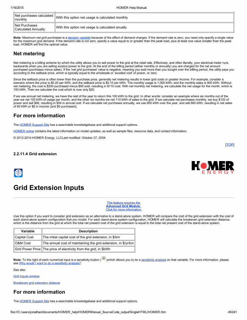
1/16/2015 HOMER Help Manual
file:///C:/users/jonathan/documents/HOMER_help/HOMERManual_SourceCode_output/SingleHTML/HOMER.htm 45/241
Net purchases calculatedmonthly With this option net usage is calculated monthly
Net PurchasesCalculated Annually With this option net usage is calculated anually
Note: Maximum net grid purchases is a decision variable because of the effect of demand charges. If the demand rate is zero, you need only specify a single valuefor the maximum grid demand. If the demand rate is not zero, specify a value equal to or greater than the peak load, plus at least one value smaller than the peakload. HOMER will find the optimal value.
Net meteringNet metering is a billing scheme by which the utility allows you to sell power to the grid at the retail rate. Effectively, and often literally, your electrical meter runsbackwards when you are selling surplus power to the grid. At the end of the billing period (either monthly or annually) you are charged for the net amountpurchased (purchases minus sales). If the 'net grid purchases' value is negative, meaning you sold more than you bought over the billling period, the utility pays youaccording to the sellback price, which is typically equal to the wholesale or 'avoided cost' of power, or zero.
Since the sellback price is often lower than the purchase price, generally net metering results in lower grid costs or greater income. For example, consider ascenario where the price is $0.20 per kWh, and the sellback price is $0.10 per kWh. The monthly usage is 1,000 kWh, and the monthly sales is 900 kWh. Withoutnet metering, the cost is $200 purchased minus $90 sold, resulting in $110 cost. With net monthly net metering, we calculate the net usage for the month, which is100 kWh. Then we calculate the cost which is now only $20.
If we use annual net metering, we have the rest of the year to return this 100 kWh to the grid. In other words: consider an example where six months out of theyear we net 100 kWh of usage per month, and the other six months we net 110 kWh of sales to the grid. If we calculate net perchases monthly, we buy $120 ofpower and sell $66, resulting in $54 in annual cost. If we calculate net purchases annually, we use 600 kWh over the year, and sell 660 kWh, resulting in net salesof 60 kWh or $6 in income (and $0 purchased).
For more informationThe HOMER Support Site has a searchable knowledgebase and additional support options.
HOMER online contains the latest information on model updates, as well as sample files, resource data, and contact information.
© 20122014 HOMER Energy, LLCLast modified: October 27, 2004
[TOP]
2.2.11.4 Grid extension
Grid Extension Inputs
This feature requires the Advanced Grid Module. Click for more information.
Use this option if you want to consider grid extension as an alternative to a standalone system. HOMER will compare the cost of the grid extension with the cost ofeach standalone system configuration that you model. For each standalone system configuration, HOMER will calculate the breakeven grid extension distance,which is the distance from the grid at which the total net present cost of the grid extension is equal to the total net present cost of the standalone system.
Variable DescriptionCapital Cost The initial capital cost of the grid extension, in $/km
O&M Cost The annual cost of maintaining the grid extension, in $/yr/km
Grid Power Price The price of electricity from the grid, in $kWh
Note: To the right of each numerical input is a sensitivity button ( )which allows you to do a sensitivity analysis on that variable. For more information, pleasesee Why would I want to do a sensitivity analysis?
See also
Grid Inputs window
Breakeven grid extension distance
For more informationThe HOMER Support Site has a searchable knowledgebase and additional support options.
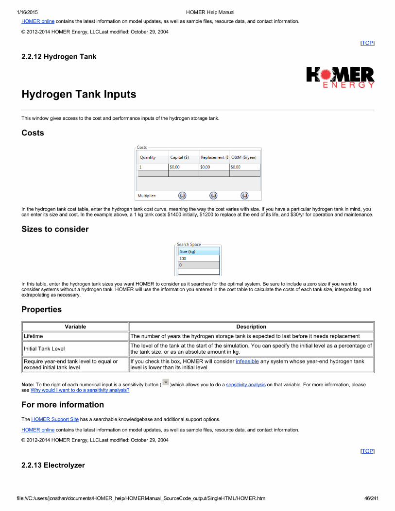
1/16/2015 HOMER Help Manual
file:///C:/users/jonathan/documents/HOMER_help/HOMERManual_SourceCode_output/SingleHTML/HOMER.htm 46/241
HOMER online contains the latest information on model updates, as well as sample files, resource data, and contact information.
© 20122014 HOMER Energy, LLCLast modified: October 29, 2004
[TOP]
2.2.12 Hydrogen Tank
Hydrogen Tank Inputs
This window gives access to the cost and performance inputs of the hydrogen storage tank.
Costs
In the hydrogen tank cost table, enter the hydrogen tank cost curve, meaning the way the cost varies with size. If you have a particular hydrogen tank in mind, youcan enter its size and cost. In the example above, a 1 kg tank costs $1400 initially, $1200 to replace at the end of its life, and $30/yr for operation and maintenance.
Sizes to consider
In this table, enter the hydrogen tank sizes you want HOMER to consider as it searches for the optimal system. Be sure to include a zero size if you want toconsider systems without a hydrogen tank. HOMER will use the information you entered in the cost table to calculate the costs of each tank size, interpolating andextrapolating as necessary.
Properties
Variable DescriptionLifetime The number of years the hydrogen storage tank is expected to last before it needs replacement
Initial Tank Level The level of the tank at the start of the simulation. You can specify the initial level as a percentage ofthe tank size, or as an absolute amount in kg.
Require yearend tank level to equal orexceed initial tank level
If you check this box, HOMER will consider infeasible any system whose yearend hydrogen tanklevel is lower than its initial level
Note: To the right of each numerical input is a sensitivity button ( )which allows you to do a sensitivity analysis on that variable. For more information, pleasesee Why would I want to do a sensitivity analysis?
For more informationThe HOMER Support Site has a searchable knowledgebase and additional support options.
HOMER online contains the latest information on model updates, as well as sample files, resource data, and contact information.
© 20122014 HOMER Energy, LLCLast modified: October 29, 2004
[TOP]
2.2.13 Electrolyzer
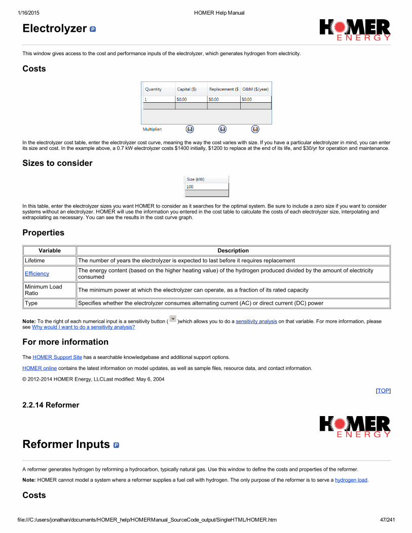
1/16/2015 HOMER Help Manual
file:///C:/users/jonathan/documents/HOMER_help/HOMERManual_SourceCode_output/SingleHTML/HOMER.htm 47/241
Electrolyzer
This window gives access to the cost and performance inputs of the electrolyzer, which generates hydrogen from electricity.
Costs
In the electrolyzer cost table, enter the electrolyzer cost curve, meaning the way the cost varies with size. If you have a particular electrolyzer in mind, you can enterits size and cost. In the example above, a 0.7 kW electrolyzer costs $1400 initially, $1200 to replace at the end of its life, and $30/yr for operation and maintenance.
Sizes to consider
In this table, enter the electrolyzer sizes you want HOMER to consider as it searches for the optimal system. Be sure to include a zero size if you want to considersystems without an electrolyzer. HOMER will use the information you entered in the cost table to calculate the costs of each electrolyzer size, interpolating andextrapolating as necessary. You can see the results in the cost curve graph.
Properties
Variable DescriptionLifetime The number of years the electrolyzer is expected to last before it requires replacement
Efficiency The energy content (based on the higher heating value) of the hydrogen produced divided by the amount of electricityconsumed
Minimum LoadRatio The minimum power at which the electrolyzer can operate, as a fraction of its rated capacity
Type Specifies whether the electrolyzer consumes alternating current (AC) or direct current (DC) power
Note: To the right of each numerical input is a sensitivity button ( )which allows you to do a sensitivity analysis on that variable. For more information, pleasesee Why would I want to do a sensitivity analysis?
For more informationThe HOMER Support Site has a searchable knowledgebase and additional support options.
HOMER online contains the latest information on model updates, as well as sample files, resource data, and contact information.
© 20122014 HOMER Energy, LLCLast modified: May 6, 2004
[TOP]
2.2.14 Reformer
Reformer Inputs
A reformer generates hydrogen by reforming a hydrocarbon, typically natural gas. Use this window to define the costs and properties of the reformer.
Note: HOMER cannot model a system where a reformer supplies a fuel cell with hydrogen. The only purpose of the reformer is to serve a hydrogen load.
Costs

1/16/2015 HOMER Help Manual
file:///C:/users/jonathan/documents/HOMER_help/HOMERManual_SourceCode_output/SingleHTML/HOMER.htm 48/241
In the cost table, enter the reformer cost curve, meaning the way the cost varies with size.
Note that the capital cost is the initial purchase price, the replacement cost is the cost of replacing the reformer at the end of its lifetime (relevant only if the projectlifetime exceeds the reformer lifetime), and the operating and maintenance cost is the annual cost of operating and maintaining the reformer.
Sizes to consider
In this table, enter the reformer sizes you want HOMER to consider as it searches for the optimal system. Be sure to include a zero size if you want to considersystems without a reformer. HOMER will use the information you entered in the cost table to calculate the costs of each reformer size, interpolating andextrapolating as necessary. You can see the results in the cost curve graph.
Tip: You can also access the values in this table using the Search Space window.
Performance parameters
The fuel dropdown box contains all the fuels stored in your component library. Choose the appropriate fuel from this list. To see the properties of the selected fuel,click the Details button.
You can create a new fuel type by clicking the New button. The new fuel type will be added to your component library. You can also remove a fuel type from thecomponent library by clicking on the Delete button. Note that additions and deletions from the component library are canceled if you close the Reformer Inputswindow with the Cancel button.
Variable DescriptionEfficiency The efficiency with which the reformer converts the fuel to hydrogen, in %
Economic parameters
Variable DescriptionLifetime The number of years the reformer will last
Delivery Cost The cost of transporting the hydrogen produced by the reformer to the site of use, in $/kg/km
Tip: You do not need to input cost data if you do not want to consider delivery cost. HOMER will assume the delivery cost to be zero if there is no delivery costentered.
Note: To the right of each numerical input is a sensitivity button ( )which allows you to do a sensitivity analysis on that variable. For more information, pleasesee Why would I want to do a sensitivity analysis?
For more informationThe HOMER Support Site has a searchable knowledgebase and additional support options.
HOMER online contains the latest information on model updates, as well as sample files, resource data, and contact information.
© 20122014 HOMER Energy, LLCLast modified: October 29, 2004
[TOP]
2.3 Resources

1/16/2015 HOMER Help Manual
file:///C:/users/jonathan/documents/HOMER_help/HOMERManual_SourceCode_output/SingleHTML/HOMER.htm 49/241
Resources
In HOMER, a "resource" is anything coming from outside the system that is used by a component to generate electric or thermal energy.
Resource ComponentsSolar GHI Resource PV (Flat Panel)Solar DNI Resource PV (Concentrating)Temperature Resource PV (Consider temperature effects)Wind Resource Wind TurbineHydro Resource Hydro ComponentFuel Resource GeneratorBiomass Resource Generator (Biogas)
For more informationThe HOMER Support Site has a searchable knowledgebase and additional support options.
HOMER online contains the latest information on model updates, as well as sample files, resource data, and contact information.
© 20122014 HOMER Energy, LLCLast modified: May 6, 2004
[TOP]
2.3.1 Solar GHI Resource
Solar GHI Resource
The Global Horizontal Irradiation (GHI) Resource is used to calculate flat panel PV array output. GHI is the sum of beam radiation (also called direct normalirradiance or DNI), diffuse irradiance, and groundreflected radiation. For more details on the equations that determine the incident radiation based on the GHI, seeHow HOMER Calculates the Radiation Incident on the PV Array.
Note: For concentrating PV, enter a Solar DNI Resource, not GHI. Concentrating PV only captures DNI, the beam radiation component of GHI, and so uses theSolar DNI resource.
The Solar Resource inputs window can be reached from the resources tab by clicking the icon in the resources tab of the navigation ribbon at the top of the
HOMER window or by clicking the button at the top of the PV inputs pane.
Choose LocaleIf you select a location on the map in the home page, the latitude and longitude will appear here. Otherwise, you can enter the latitude and longitude manually.Select the time zone by clicking the "Update" button or by choosing from the drop down menu. HOMER uses the location for several aspects of the PV powercalculation, so it is important to specify this even if you are not downloading solar data.
Choose Data Source
The baseline data is a oneyear time series representing the average global solar radiation on the horizontal surface, expressed in kWh/m2, for each time step ofthe year. HOMER displays the monthly average radiation and clearness index of the baseline data in the solar resource table and graph.
There are two ways to create baseline data: you can use HOMER to synthesize hourly data from monthly averages, or you can import time series radiation datafrom a file. If you are looking for solar data, see Finding data to run HOMER.
Enter Monthly AveragesSolar resource data can be input via the monthly solar radiation table. You can enter the monthly data manually, or you can download it from the HOMER website.
To enter twelve average monthly values into the solar resource table manually, you can input either solar radiation (in kWh/m2 per day) or clearness index. You donot have to enter both; HOMER calculates one from the other using the latitude.
To download solar data from the HOMER Energy website, simply click the "Download" button. This will automatically fill in the twelve monthly average values foryou based on the latitude and longitude.

1/16/2015 HOMER Help Manual
file:///C:/users/jonathan/documents/HOMER_help/HOMERManual_SourceCode_output/SingleHTML/HOMER.htm 50/241
Once you have values in the monthly solar radiation table, either by manual entry or download, HOMER builds a set of 8,760 solar radiation values, or one for eachhour of the year. HOMER creates the synthesized values using the Graham algorithm, which results in a data sequence that has realistic daytoday and hourtohour variability and autocorrelation. For more information please see the article on synthetic solar data.
Import Solar DataYou can prepare your own text file that contains the solar radiation data in each time step for a complete year.
Tip: You can import data with any time step down to one minute. HOMER detects the time step when you import the data file. For example, if the data file contains8760 lines, HOMER will assume that it contains hourly data. If the data file contains 52,560 lines, HOMER will assume that it contains 10minute data.
The data file must contain a single value on each line, where each line corresponds to one time step. Each value in the file represents the average solar radiation(in kW/m2) for that time step. The first time step starts at midnight on January 1st. A sample input file appears below.
Click to open the text file. You can import a text file with any extension.
When you import data from a text file, HOMER makes a copy of the data set and integrates it with the HOMER (.homer) file. Once the data is part of the HOMERfile, HOMER no longer refers to the original text file. If you modify data in the original file, you must import the modified file in order for the modification to beincluded in the HOMER file. After you import a data file, HOMER calculates monthly average radiation and clearness index values and displays them in the tableand graph. HOMER also displays the name of the imported data file in the title of the graph.
If you enter new monthly solar radiation values after importing data from a file, HOMER discards the data from the imported file and synthesizes new data basedon the twelve new monthly averages. You can edit synthesized data by changing values in the solar resource table. To edit values from an imported file, you mustedit the file directly and then import the modified file, as described above.
Scaled data for simulation
HOMER uses scaled data for calculations. To create scaled data, HOMER multiplies each of the values in the baseline data by a common factor that results in anannual average value equal to the value that you specify in Scaled Annual Average. To determine the value of this factor, HOMER divides the scaled annualaverage by the baseline annual average solar radiation. The scaled data retains the shape and statistical characteristics of the baseline data, but may differ inmagnitude. The default value for the scaled annual average is the baseline annual average solar radiation. When the two values are equal, the scaled data andbaseline are identical. HOMER inteprets a scaled annual average of zero to mean that there is no solar radiation.
Two reasons to use a scaled annual average that is different from the baseline annual average are for unit conversion or to perform a sensitivity analysis.
An example of using the scaled annual average for unit conversion is to convert data from an imported file that contains solar radiation data expressed in Wh/m2
rather than kWh/m2. If the baseline annual average is 4800 Wh/m2, you should enter 4.8 in Scaled Annual Average, so that the scaled data is equivalent to thebaseline data, but expressed in kWh/m2: 1 kWh/m2 = 1000 Wh/m2.
Note: To the right of the Scaled Annual Average input is a sensitivity button ( )which allows you to do a sensitivity analysis on that variable. For moreinformation, please see Why would I want to do a sensitivity analysis?
See also
Generating synthetic solar data
Finding data to run HOMER
The solar resource section of Recommended Reading
Why do I have to scale load and resource data?

1/16/2015 HOMER Help Manual
file:///C:/users/jonathan/documents/HOMER_help/HOMERManual_SourceCode_output/SingleHTML/HOMER.htm 51/241
For more informationThe HOMER Support Site has a searchable knowledgebase and additional support options.
HOMER online contains the latest information on model updates, as well as sample files, resource data, and contact information.
© 20122014 HOMER Energy, LLCLast modified: January 22, 2010
[TOP]
2.3.2 Solar DNI Resource
Solar DNI Resource
The Direct Normal Irradiance (DNI) Resource is used to calculate concetrating PV output. Concentrating PV uses optics to concentrate the solar radiation in a waythat only captures the direct beam radiation (also called DNI) and does not capture the diffuse or reflected components of the incident solar radiation.
Note: For a flat panel PV, enter a Solar GHI resource, not DNI. Flat panel PV captures direct, diffuse, and reflected radiation, and so uses the Solar GHI resourceto calculate output.
The Solar DNI Resource inputs window can be reached from the resources tab by clicking the icon in the resources tab of the navigation ribbon at the top of the
HOMER window or by clicking the button at the top of the PV inputs pane.
Choose LocaleYou can select a location on the map in the home page.
Importing Solar DataThe Solar DNI resource can only by specified by importing a timeseries data file. See the help article Finding data to run HOMER for a list of sources for solardata.
You can prepare your own text file that contains the solar radiation data in each time step for a complete year.
Tip: You can import data with any time step down to one minute. HOMER detects the time step when you import the data file. For example, if the data file contains8760 lines, HOMER will assume that it contains hourly data. If the data file contains 52,560 lines, HOMER will assume that it contains 10minute data.
The data file must contain a single value on each line, where each line corresponds to one time step. Each value in the file represents the average solar radiation(in kW/m2) for that time step. The first time step starts at midnight on January 1st. A sample input file appears below.
Click to open the text file. You can import a text file with any extension.
When you import data from a text file, HOMER makes a copy of the data set and integrates it with the HOMER (.homer) file. Once the data is part of the HOMER

1/16/2015 HOMER Help Manual
file:///C:/users/jonathan/documents/HOMER_help/HOMERManual_SourceCode_output/SingleHTML/HOMER.htm 52/241
file, HOMER no longer refers to the original text file. If you modify data in the original file, you must import the modified file in order for the modification to beincluded in the HOMER file. After you import a data file, HOMER calculates monthly average radiation and clearness index values and displays them in the tableand graph. HOMER also displays the name of the imported data file in the title of the graph.
If you enter new monthly solar radiation values after importing data from a file, HOMER discards the data from the imported file and synthesizes new data basedon the twelve new monthly averages. You can edit synthesized data by changing values in the solar resource table. To edit values from an imported file, you mustedit the file directly and then import the modified file, as described above.
Scaled data for simulation
HOMER uses scaled data for calculations. To create scaled data, HOMER multiplies each of the values in the baseline data by a common factor that results in anannual average value equal to the value that you specify in Scaled Annual Average. To determine the value of this factor, HOMER divides the scaled annualaverage by the baseline annual average solar radiation. The scaled data retains the shape and statistical characteristics of the baseline data, but may differ inmagnitude. The default value for the scaled annual average is the baseline annual average solar radiation. When the two values are equal, the scaled data andbaseline are identical. HOMER inteprets a scaled annual average of zero to mean that there is no solar radiation.
Two reasons to use a scaled annual average that is different from the baseline annual average are for unit conversion or to perform a sensitivity analysis.
An example of using the scaled annual average for unit conversion is to convert data from an imported file that contains solar radiation data expressed in Wh/m2
rather than kWh/m2. If the baseline annual average is 4800 Wh/m2, you should enter 4.8 in Scaled Annual Average, so that the scaled data is equivalent to thebaseline data, but expressed in kWh/m2: 1 kWh/m2 = 1000 Wh/m2.
Note: To the right of the Scaled Annual Average input is a sensitivity button ( )which allows you to do a sensitivity analysis on that variable. For moreinformation, please see Why would I want to do a sensitivity analysis?
See also
Generating synthetic solar data
Finding data to run HOMER
The solar resource section of Recommended Reading
Why do I have to scale load and resource data?
For more informationThe HOMER Support Site has a searchable knowledgebase and additional support options.
HOMER online contains the latest information on model updates, as well as sample files, resource data, and contact information.
© 20122014 HOMER Energy, LLCLast modified: January 22, 2010
[TOP]
2.3.3 Temperature Resource
Temperature Resource
The Temperature Resources window can be reached by selecting the Resouces tab and clicking the temperature icon.
Use this window to specify the ambient temperature for the year. Enter twelve monthly numbers or import a time series data file. If you import a TMY2 or TMY3 file,HOMER will extract the dry bulb temperature.
If you enter a scaled average different from the average of the baseline data, HOMER will offset the temperature data to correspond to the average value that youenter.
HOMER uses the ambient temperature to calculate the PV cell temperature, as described in the article on how HOMER calculates the PV cell temperature.
The Plot button allows you to view the scaled data in several graphical formats. The Export button allows you to export the scaled data to a text file.
See also:
How HOMER calculates the PV cell temperature
For more informationThe HOMER Support Site has a searchable knowledgebase and additional support options.

1/16/2015 HOMER Help Manual
file:///C:/users/jonathan/documents/HOMER_help/HOMERManual_SourceCode_output/SingleHTML/HOMER.htm 53/241
HOMER online contains the latest information on model updates, as well as sample files, resource data, and contact information.
© 20122014 HOMER Energy, LLCLast modified: November 21, 2007
[TOP]
2.3.4 Wind Resource
Wind Resource
The Wind Resource inputs window can be reached from the Wind Turbine inputs window by clicking the button at the top of the screen or from the
Resources tab by using the button.
You can use this window to describe the available wind resource. HOMER will use this data to calculate the output of the wind turbine in each time step. Thiswindow also provides access to the following tabs:
Parameters: Variables related to altitudeVariation with Height: Parameters describing wind shear and the wind velocity's vertical profileAdvanced Parameters: Parameters controlling variation of the wind over time
If you are looking for wind resource data, see Finding data to run HOMER
Baseline dataThe baseline data is a oneyear time series representing the average wind speed, expressed in meters per second, for each time step of the year. HOMERdisplays the monthly averages calculated from the baseline data in the wind resource table and graph.
You can create baseline data either by using HOMER to synthesize time series data, or by importing time series data from a file.
To synthesize data, you must enter twelve average wind speed values: one for each month of the year. You can also edit the four advanced parameters. Entereach month's average wind speed (m/s) in the table. As you enter values in the table, HOMER synthesizes time series data with the statistical characteristics youhave specified. For more information please see the article on synthetic wind data.
Scaled data for simulation
HOMER uses scaled data for calculations. To create scaled data, HOMER multiplies each of the baseline data values by a common factor that results in an annualaverage value equal to the value that you specify in Scaled annual average. To determine the value of this factor, HOMER divides the scaled annual average bythe baseline annual average. The scaled data retains the shape and statistical characteristics of the baseline data, but may differ in magnitude. The default valuefor the scaled annual average is the baseline annual average. When the two values are equal, the scaled data and baseline are identical. HOMER inteprets ascaled annual average of zero to mean that there is no wind resource.
Two reasons to use a scaled annual average that is different from the baseline annual average are for unit conversion or to perform a sensitivity analysis.
An example of using the scaled annual average for unit conversion is to convert data from an imported file that contains wind speed expressed in kilometers perhour. If the baseline annual average is 20 km/hr, you should enter 5.56 in Scaled annual average, so that the scaled data is equivalent to the baseline data, butexpressed in m/s rather than km/hr: 1 m/s = 3.6 km/hr; 5.56 m/s = 20 km/hr.
Note: To the right of the Scaled Annual Averages input is a sensitivity button ( )which allows you to do a sensitivity analysis on that variable. For moreinformation, please see Why would I want to do a sensitivity analysis?
Importing Wind Speed DataTo import a file, you must prepare a text file that contains the wind speed in each time step for a complete year.
Tip: You can import data with any time step down to one minute. HOMER detects the time step when you import the data file. For example, if the data file contains8760 lines, HOMER will assume that it contains hourly data. If the data file contains 52,560 lines, HOMER will assume that it contains 10minute data.
The data file must contain a single value on each line, where each line corresponds to one time step. Each value in the file represents the average wind speed (inm/s) for that time step. The first time step starts at midnight on January 1st. A sample input file appears below.

1/16/2015 HOMER Help Manual
file:///C:/users/jonathan/documents/HOMER_help/HOMERManual_SourceCode_output/SingleHTML/HOMER.htm 54/241
When you import data from a text file, HOMER makes a copy of the data set and integrates it with the HOMER (.hmr) file. Once the data is part of the HOMER file,HOMER no longer refers to the original text file. If you modify data in the original file, you must import the modified file in order for the modification to be included inthe HOMER file. After you import a data file, HOMER calculates twelve monthly average wind speed values and displays them in the table and graph. HOMERalso displays the name of the imported data file in the title of the graph. HOMER calculates the four advanced parameters from the imported data and displaysthem (readonly) in the text boxes.
Pro: If you click Enter monthly averages after importing data from a file, HOMER discards the data from the imported file and synthesizes new data based on thetwelve monthly average wind speed values and four advanced parameters it calculated from the imported data. You can edit synthesized data by changing valuesin the monthly wind speed table. To edit values from an imported file, you must edit the file directly and then import the modified file, as described above.
See also:
Generating synthetic wind data
Finding data to run HOMER
The wind resource section of Recommended Reading
Why do I have to scale load and resource data?
How HOMER calculates wind turbine power output
For more informationThe HOMER Support Site has a searchable knowledgebase and additional support options.
HOMER online contains the latest information on model updates, as well as sample files, resource data, and contact information.
© 20122014 HOMER Energy, LLCLast modified: July 3, 2013
[TOP]
2.3.4.1 Wind Resource Parameters
Wind Resource Parameters
The Parameters tab in the Wind Resource window gives you access to the following variables:
Variable DescriptionAltitude The altitude in meters above sea levelAnemometer Height The height above ground at which the wind speed data were measured, in meters
For more informationThe HOMER Support Site has a searchable knowledgebase and additional support options.
HOMER online contains the latest information on model updates, as well as sample files, resource data, and contact information.
© 20122014 HOMER Energy, LLCLast modified: July 15, 2013
[TOP]
2.3.4.2 Wind Resource Variation with Height

1/16/2015 HOMER Help Manual
file:///C:/users/jonathan/documents/HOMER_help/HOMERManual_SourceCode_output/SingleHTML/HOMER.htm 55/241
Wind Resource Variation with Height
Use this window to describe the way the wind speed increases with height above ground. HOMER uses this information to calculate the wind speed at the hubheight of the wind turbine.
Groundlevel obstacles such as vegetation, buildings, and topographic features tend to slow the wind near the surface. Since the effect of these obstaclesdecreases with height above ground, wind speeds tend to increase with height above ground. This variation of wind speed with height is called wind shear. Windenergy engineers typically model wind shear using one of two mathematical models, the logarithmic profile or the power law profile.
Logarithmic profileThe logarithmic profile (or log law) assumes that the wind speed is proportional to the logarithm of the height above ground. The following equation therefore givesthe ratio of the wind speed at hub height to the wind speed at anemometer height:
where:Uhub = the wind speed at the hub height of the wind turbine [m/s]Uanem = the wind speed at anemometer height [m/s]zhub = the hub height of the wind turbine [m]zanem = the anemometer height [m]z0 = the surface roughness length [m]ln(..) = the natural logarithm
The surface roughness length is a parameter that characterizes the roughness of the surrounding terrain. The table below contains representative surfaceroughness lengths taken from Manwell, McGowan, and Rogers:
Terrain Description z0Very smooth, ice or mud 0.00001 mCalm open sea 0.0002 mBlown sea 0.0005 mSnow surface 0.003 mLawn grass 0.008 mRough pasture 0.010 mFallow field 0.03 mCrops 0.05 mFew trees 0.10 mMany trees, few buildings 0.25 mForest and woodlands 0.5 mSuburbs 1.5 mCity center, tall buildings 3.0 m
Power law profileThe power law profile assumes that the ratio of wind speeds at different heights is given by the following equation:
where:
Uhub = the wind speed at the hub height of the wind turbine [m/s]Uanem = the wind speed at anemometer height [m/s]zhub = the hub height of the wind turbine [m]zanem = the anemometer height [m]a = the power law exponent
The power law exponent is a dimensionless parameter. Foundational research in fluid mechanics showed that its value is equal to 1/7 for turbulent flow over a flatplate. Wind speed researchers have found that in practice the power law exponent depends on terrain roughness, atmospheric stability, and several other factors.
See also:
Wind resource inputs
Anemometer height

1/16/2015 HOMER Help Manual
file:///C:/users/jonathan/documents/HOMER_help/HOMERManual_SourceCode_output/SingleHTML/HOMER.htm 56/241
Wind turbine hub height
How HOMER calculates wind turbine power output
For more informationThe HOMER Support Site has a searchable knowledgebase and additional support options.
HOMER online contains the latest information on model updates, as well as sample files, resource data, and contact information.
© 20122014 HOMER Energy, LLCLast modified: October 8, 2009
[TOP]
2.3.4.3 Wind Resource Advanced Parameters
Advanced Parameters
The Advanced Inputs tab in the Wind Resource window gives you access to the following variables:
Variable DescriptionWeibull k A measure of the longterm distribution of wind speedsAutocorrelation Factor A measure of the hourtohour randomness of the wind speedDiurnal Pattern Strength A measure of how strongly the wind speed depends on the time of dayHour of Peak Wind Speed The time of day that tends to be windiest on average
For more informationThe HOMER Support Site has a searchable knowledgebase and additional support options.
HOMER online contains the latest information on model updates, as well as sample files, resource data, and contact information.
© 20122014 HOMER Energy, LLCLast modified: July 15, 2013
[TOP]
2.3.5 Hydro Resource
Hydro Resource
This feature requires the Hydro Module.
Click for more information.
Use the Hydro Resource Inputs window to describe the stream flow available to the hydro turbine. HOMER uses this data to calculate the output of the hydroturbine in each time step.
Baseline dataThe baseline data is a oneyear time series representing the average stream flow, expressed in liters per second, for each time step of the year. HOMER displaysthe monthly averages calculated from the baseline data in the stream flow table and graph.
There are two ways to create baseline data: you can use HOMER to synthesize hourly data, or you can import time series data from a file.
To synthesize data, you must enter twelve average stream flow values: one for each month of the year. Enter each month's average stream flow (L/s) in theappropriate row on the stream flow table. As you enter values in the table, HOMER builds a set of 8,760 values, or one stream flow value for each hour of the year.HOMER creates the synthesized values by assuming that the stream flow is constant throughout each month; HOMER simply assigns the monthly average valueto each hour in that month.
To import a file, you must prepare a text file that contains the stream flow in each time step for a complete year.

1/16/2015 HOMER Help Manual
file:///C:/users/jonathan/documents/HOMER_help/HOMERManual_SourceCode_output/SingleHTML/HOMER.htm 57/241
Tip: You can import data with any time step down to one minute. HOMER detects the time step when you import the data file. For example, if the data file contains8760 lines, HOMER will assume that it contains hourly data. If the data file contains 52,560 lines, HOMER will assume that it contains 10minute data.
The data file must contain a single value on each line, where each line corresponds to one time step. Each value in the file represents the average stream flow (inL/s) for that time step. The first time step starts at midnight on January 1st. A sample input file appears below.
When you import data from a text file, HOMER makes a copy of the data set and integrates it with the HOMER (.hmr) file. Once the data is part of the HOMER file,HOMER no longer refers to the original text file. If you modify data in the original file, you must import the modified file in order for the modification to be included inthe HOMER file. After you import a data file, HOMER calculates twelve monthly average stream flow values and displays them in the table and graph. HOMERalso displays the name of the imported data file in the title of the stream flow graph.
If you click Enter monthly averages after importing data from a file, HOMER discards the data from the imported file and synthesizes new data based on the twelvemonthly average values it calculated from the imported data. You can edit synthesized data by changing values in the stream flow table. To edit values from animported file, you must edit the file directly and then import the modified file, as described above.
Scaled data for simulation
HOMER uses scaled data for calculations. To create scaled data, HOMER multiplies each of the baseline data values by a common factor that results in an annualaverage value equal to the value that you specify in Scaled annual average. To determine the value of this factor, HOMER divides the scaled annual average bythe baseline annual average. The scaled data retains the shape and statistical characteristics of the baseline data, but may differ in magnitude. The default valuefor the scaled annual average is the baseline annual average. When the two values are equal, the scaled data and baseline are identical. HOMER inteprets ascaled annual average of zero to mean that there is no stream flow.
Two reasons to use a scaled annual average that is different from the baseline annual average are for unit conversion or to perform a sensitivity analysis.
An example of using the scaled annual average for unit conversion is to convert data from an imported file that contains stream flow data expressed in US gallonsper minute. If the baseline annual average is 90 gal/min, you should enter 5.68 in Scaled annual average, so that the scaled data is equivalent to the baseline data,but expressed in L/s rather than U.S. gallons per hour: 1 L/s = 15.85 gal/min; 5.68 L/s = 90 gal/min.
Another reason to scale the baseline data is to do a sensitivity analysis on the hydro resource. Click the sensitivities button (to the right of the text box) to entermultiple values for a sensitivity analysis.
The Plot button allows you to view the scaled data in several graphical formats. The Export button allows you to export the scaled data to a text file.
See also:
The hydro section of Recommended Reading
Why do I have to scale load and resource data?
For more informationThe HOMER Support Site has a searchable knowledgebase and additional support options.
HOMER online contains the latest information on model updates, as well as sample files, resource data, and contact information.
© 20122014 HOMER Energy, LLCLast modified: January 22, 2010
[TOP]
2.3.6 Fuel Resource
Fuel Resource
When specifying a generator component, you must select a fuel. Several common fuels are already built in to the library.

1/16/2015 HOMER Help Manual
file:///C:/users/jonathan/documents/HOMER_help/HOMERManual_SourceCode_output/SingleHTML/HOMER.htm 58/241
See also:
Create a New Fuel
For more informationThe HOMER Support Site has a searchable knowledgebase and additional support options.
HOMER online contains the latest information on model updates, as well as sample files, resource data, and contact information.
© 20122014 HOMER Energy, LLCLast modified: November 21, 2007
[TOP]
2.3.7 Biomass Resource
Biomass Resource
This feature requires the Biomass Module.
Click for more information.
HOMER assumes the biomass feedstock is fed into a gasifier to create biogas. One or more generators then consume the biogas to produce electricity (andoptionally heat). Use the Biomass Resource Inputs window to describe the availability of biomass feedstock. HOMER uses this data to calculate (in each time stepof the year) the amount of biogas that can be supplied by the gasifier to the biogasfueled generator(s).
Baseline dataThe baseline data is a oneyear time series representing the average biomass feedstock availability, expressed in kilograms, for each time step of the year.HOMER displays the monthly averages calculated from the baseline data in the biomass resource table and graph.
There are two ways to create baseline data: you can use HOMER to synthesize hourly data from monthly averages, or you can import time series data from a file.
To synthesize data, you must enter twelve average values of biomass availability: one for each month of the year. Enter each month's average biomass availability(in tonnes per day) in the appropriate row of the biomass resource table. As you enter values in the table, HOMER builds a set of 8,760 values, or one value foreach hour of the year. HOMER creates the synthesized values by assuming that the biomass availability is constant throughout each month; HOMER simplyassigns the monthly average value to each hour in that month.
To import a file, you must prepare a text file that contains the biomass feedstock availability in each time step for a complete year.
Tip: You can import data with any time step down to one minute. HOMER detects the time step when you import the data file. For example, if the data file contains8760 lines, HOMER will assume that it contains hourly data. If the data file contains 52,560 lines, HOMER will assume that it contains 10minute data.
The data file must contain a single value on each line, where each line corresponds to one time step. Each value in the file represents the biomass feedstockavailability (in kilograms) for that time step. The first time step starts at midnight on January 1st. A sample input file appears below.
When you import data from a text file, HOMER makes a copy of the data set and integrates it with the HOMER (.hmr) file. Once the data is part of the HOMER file,HOMER no longer refers to the original text file. If you modify data in the original file, you must import the modified file in order for the modification to be included inthe HOMER file. After you import a data file, HOMER calculates twelve monthly average biomass availability values and displays them in the table and graph.HOMER also displays the name of the imported data file in the title of the biomass resource graph.
If you click Enter monthly averages after importing data from a file, HOMER discards the data from the imported file and synthesizes new data based on the twelvemonthly average values it calculated from the imported data. You can edit synthesized data by changing values in the biomass resource table. To edit values froman imported file, you must edit the file directly and then import the modified file, as described above.

1/16/2015 HOMER Help Manual
file:///C:/users/jonathan/documents/HOMER_help/HOMERManual_SourceCode_output/SingleHTML/HOMER.htm 59/241
Properties
Variable DescriptionAverage cost The average cost per tonne of the biomass feedstock.
Carbon content The carbon content of the biomass feedstock as a massbased percentage.
Gasification ratio The ratio of biogas generated to biomass feedstock consumed in the gasifier.
LHV of biogas The energy content (lower heating value) of the biogas produced by the gasifier.
Scaled data for simulation
HOMER uses scaled data for calculations. To create scaled data, HOMER multiplies each of the baseline data values by a common factor that results in an annualaverage value equal to the value that you specify in Scaled annual average. To determine the value of this factor, HOMER divides the scaled annual average bythe baseline annual average. The scaled data retains the shape and statistical characteristics of the baseline data, but may differ in magnitude. The default valuefor the scaled annual average is the baseline annual average. When the two values are equal, the scaled data and baseline are identical. HOMER inteprets ascaled annual average of zero to mean that there is no biomass resource.
Two reasons to use a scaled annual average that is different from the baseline annual average are for unit conversion or to perform a sensitivity analysis.
The Plot button allows you to view the scaled data in several graphical formats. The Export button allows you to export the scaled data to a text file.
Note: To the right of each numerical input is a sensitivity button ( )which allows you to do a sensitivity analysis on that variable. For more information, pleasesee Why would I want to do a sensitivity analysis?
See also:
The biomass section of Recommended Reading
Why do I have to scale load and resource data?
For more informationThe HOMER Support Site has a searchable knowledgebase and additional support options.
HOMER online contains the latest information on model updates, as well as sample files, resource data, and contact information.
© 20122014 HOMER Energy, LLCLast modified: January 22, 2010
[TOP]
2.3.8 Hydrokinetic
Hydrokinetic Resource
Use the Hydrokinetic Resource Inputs window to describe the flow available to the hydrokinetic turbine. HOMER uses this data to calculate the output of the hydroturbine in each time step.
Baseline water speed dataThe baseline data is a oneyear time series representing the water speed, expressed in meters per second, for each time step of the year. HOMER displays themonthly averages calculated from the baseline data in the water speed table and graph.
There are two ways to create baseline data: you can enter monthly averages, or you can import time series data from a file.
To enter twelve monthly averages, enter each month's average water speed (m/s) in the appropriate row on the water speed table. As you enter values in thetable, HOMER builds a set of 8,760 values, or one water speed value for each hour of the year. HOMER creates the hourly values by assuming that the streamflow is constant throughout each month; HOMER simply assigns the monthly average value to each hour in that month.
To import a file, you must prepare a text file that contains the water speed in each time step for a complete year.
Tip: You can import data with any time step down to one minute. HOMER detects the time step when you import the data file. For example, if the data file contains8760 lines, HOMER will assume that it contains hourly data. If the data file contains 52,560 lines, HOMER will assume that it contains 10minute data.
The data file must contain a single value on each line, where each line corresponds to one time step. Each value in the file represents the average water speed (inm/s) for that time step. The first time step starts at midnight on January 1st. A sample input file appears below.
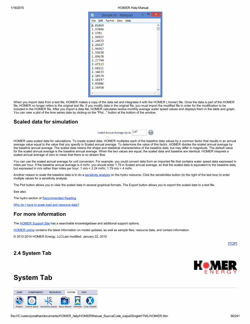
1/16/2015 HOMER Help Manual
file:///C:/users/jonathan/documents/HOMER_help/HOMERManual_SourceCode_output/SingleHTML/HOMER.htm 60/241
When you import data from a text file, HOMER makes a copy of the data set and integrates it with the HOMER (.homer) file. Once the data is part of the HOMERfile, HOMER no longer refers to the original text file. If you modify data in the original file, you must import the modified file in order for the modification to beincluded in the HOMER file. After you import a data file, HOMER calculates twelve monthly average water speed values and displays them in the table and graph.You can view a plot of the time series data by clicking on the "Plot..." button at the bottom of the window.
Scaled data for simulation
HOMER uses scaled data for calculations. To create scaled data, HOMER multiplies each of the baseline data values by a common factor that results in an annualaverage value equal to the value that you specify in Scaled annual average. To determine the value of this factor, HOMER divides the scaled annual average bythe baseline annual average. The scaled data retains the shape and statistical characteristics of the baseline data, but may differ in magnitude. The default valuefor the scaled annual average is the baseline annual average. When the two values are equal, the scaled data and baseline are identical. HOMER inteprets ascaled annual average of zero to mean that there is no stream flow.
You can use the scaled annual average for unit conversion. For example, you could convert data from an imported file that contains water speed data expressed inmiles per hour. If the baseline annual average is 4 mi/hr, you should enter 1.79 in Scaled annual average, so that the scaled data is equivalent to the baseline data,but expressed in m/s rather than miles per hour: 1 m/s = 2.24 mi/hr; 1.79 m/s = 4 mi/hr.
Another reason to scale the baseline data is to do a sensitivity analysis on the hydro resource. Click the sensitivities button (to the right of the text box) to entermultiple values for a sensitivity analysis.
The Plot button allows you to view the scaled data in several graphical formats. The Export button allows you to export the scaled data to a text file.
See also:
The hydro section of Recommended Reading
Why do I have to scale load and resource data?
For more informationThe HOMER Support Site has a searchable knowledgebase and additional support options.
HOMER online contains the latest information on model updates, as well as sample files, resource data, and contact information.
© 20122014 HOMER Energy, LLCLast modified: January 22, 2010
[TOP]
2.4 System Tab
System Tab

1/16/2015 HOMER Help Manual
file:///C:/users/jonathan/documents/HOMER_help/HOMERManual_SourceCode_output/SingleHTML/HOMER.htm 61/241
The System tab gives you access all of the menus where you can review your project and model as a whole. It is a good place to review your model and inputsbefore you calculate results. The system tab contains the following menus:
Name DescriptionProject Set Up Options that apply to the entire model: economics, system control, emissions, and constraints
Input Report create an HTMLformat report summarizing all the model inputs, and display it in a browser
Search Space View and edit the system parameters HOMER simulates to find the optimal system configuration
Sensitivity Inputs View and modify all the sensitivity variables in the model
For more informationThe HOMER Support Site has a searchable knowledgebase and additional support options.
HOMER online contains the latest information on model updates, as well as sample files, resource data, and contact information.
© 20122014 HOMER Energy, LLCLast modified: July 2, 2013
[TOP]
2.4.1 Project Set Up
Project set up
In the Project Set Up window you can set options that apply to your entire model. They are grouped onto the following tabs:
EconomicsSystem ControlEmissionsConstraints
See also
Definition of sensitivity variable
For more informationThe HOMER Support Site has a searchable knowledgebase and additional support options.
HOMER online contains the latest information on model updates, as well as sample files, resource data, and contact information.
© 20122014 HOMER Energy, LLCLast modified: October 29, 2004
[TOP]
2.4.1.1 Economics
Economic Inputs
The Economics tab under the Project Setup tab gives access to the following variables:
Variable DescriptionAnnual Real Interest Rate The discount rate used to convert between onetime costs and annualized costs, in %
Project Lifetime The number of years over which the net present cost of the project should be calculated
System Fixed Capital Cost The fixed capital cost that occurs regardless of the size or architecture of the system, in $
System Fixed O&M Cost The fixed annual costs that occur regardless of the size or architecture of the system, in $/yr
Capacity Shortage Penalty A penalty applied to the system for any capacity shortage, in $/kWh

1/16/2015 HOMER Help Manual
file:///C:/users/jonathan/documents/HOMER_help/HOMERManual_SourceCode_output/SingleHTML/HOMER.htm 62/241
Note: To the right of each numerical input is a sensitivity button ( )which allows you to do a sensitivity analysis on that variable. For more information, pleasesee Why would I want to do a sensitivity analysis?
For more informationThe HOMER Support Site has a searchable knowledgebase and additional support options.
HOMER online contains the latest information on model updates, as well as sample files, resource data, and contact information.
© 20122014 HOMER Energy, LLCLast modified: May 28, 2004
[TOP]
2.4.1.2 System Control
System Control
The System Control tab under the Project tab allows you to modify how HOMER simulates your systems.
SimulationThe simulation time step is the time step that HOMER uses to simulate the operation of each system configuration. You can set the simulation time step to anythingfrom several hours down to one minute. The simulation time step does not have to match the time step of any time series load or resource data you may haveimported. See the article on the simulation time step for details.
Dispatch Strategy InputsA dispatch strategy is a set or rules that govern the operation of the generator(s) and the battery bank. HOMER can model two dispatch strategies, cycle chargingand load following. Which is optimal depends on many factors, including the sizes of the generators and battery bank, the price of fuel, the O&M cost of thegenerators, the amount of renewable power in the system, and the character of the renewable resources. If you choose to model both, HOMER will simulate eachsystem using both dispatch strategies and you will be able to see which is optimal.
Under the load following strategy, whenever a generator is needed it produces only enough power to meet the demand. Load following tends to be optimal insystems with a lot of renewable power, when the renewable power output sometimes exceeds the load.
Under the cycle charging strategy, whenever a generator has to operate, it operates at full capacity with surplus power going to charge the battery bank. Cyclecharging tends to be optimal in systems with little or no renewable power.
If you can apply a setpoint state of charge to the cycle charging strategy, the generator(s) will not stop charging the battery bank until it reaches the specified stateof charge. The sensitivity button to the right allows you to do a sensitivity analysis on this setpoint.
Note that the dispatch strategy is abbreviated "Disp. Strgy" in the sensitivity and optimization results tables.
Generator control
Allow systems withmultiple generators
This check box controls whether HOMER considers systems that contain more than one generator. It has no effect ifyou are considering only one generator.
Multiple generatorscan operatesimultaneously
This check box only affects the operation of systems that include two or more generators on the same bus. If you checkthis box, HOMER will allow multiple generators on the same bus to operate at once whenever necessary. Otherwise,multiple generators on the same bus must take turns operating.
Allow systems withgenerator capacityless than peak load
This check box controls whether HOMER will consider systems whose total generator capacity is less than the annualpeak primary load
Other settings
Allow systemswith two typesof windturbines
This check box controls whether HOMER will simulate system configurations that contain more than one type of wind turbine. Ifyou add two types of wind turbine to the schematic and you simply wish to choose between them, then leave this checkboxunchecked. If you want HOMER to simulate systems that contain both types of turbine, then check this checkbox.
Allow excesselectricity toserve thermalload
If you check this checkbox, HOMER will assume that excess electricity serves the thermal load through a resistive heater orelectric boiler
Limit excess If you check this checkbox, HOMER will prevent the system from producing more than the allowable amount of excess thermal

1/16/2015 HOMER Help Manual
file:///C:/users/jonathan/documents/HOMER_help/HOMERManual_SourceCode_output/SingleHTML/HOMER.htm 63/241
thermal output energy
Note: To the right of each numerical input is a sensitivity button ( )which allows you to do a sensitivity analysis on that variable. For more information, pleasesee Why would I want to do a sensitivity analysis?
For more informationThe HOMER Support Site has a searchable knowledgebase and additional support options.
HOMER online contains the latest information on model updates, as well as sample files, resource data, and contact information.
© 20122014 HOMER Energy, LLCLast modified: January 22, 2010
[TOP]
2.4.1.3 Emissions
Emissions
The Emissions tab under the Project tab allows you to specify a cost penalty associated with a pollutant, or a limit on the emissions of a pollutant.
Emissions PenaltiesIf you specify a nonzero cost penalty for a particular pollutant, HOMER will add the corresponding cost to the total annual cost of the power system. For example,if you specify a cost penalty for CO2 emissions of $10 per tonne and the power system produces 15 tonnes of CO2 per year, HOMER will penalize the system byadding $150/yr to its total annual cost. The emissions cost appears in the "other O&M cost" column of the in the Costs page of the Simulation Results window.
You can specify a penalty for any of the six pollutants that HOMER tracks. To the right of each input is a sensitivity button which allows you to do a sensitivityanalysis on that variable.
In its dispatch logic, HOMER takes emissions penalties into account when comparing the costs of different dispatchable generation sources. For a simple example,consider a system containing two generators whose properties are identical except that one has a higher NOx emissions factor. If the user specifies a nonzerocost penalty for NOx emissions, then whenever HOMER must choose between operating one generator or the other, it will choose the one with the lower NOxemissions factor.
Variable DescriptionCO2 Emissions Penalty A cost penalty HOMER applies to the system's emissions of carbon dioxide, in $/ton
CO Emissions Penalty A cost penalty HOMER applies to the system's emissions of carbon monoxide, in $/ton
HC Emissions Penalty A cost penalty HOMER applies to the system's emissions of unburned hydrocarbons, in $/ton
PM Emissions Penalty A cost penalty HOMER applies to the system's emissions of particulate matter, in $/ton
SO2 Emissions Penalty A cost penalty HOMER applies to the system's emissions of sulfur dioxide, in $/ton
NOx Emissions Penalty A cost penalty HOMER applies to the system's emissions of nitrogen oxides, in $/ton
Limits on EmissionsIf you specify a limit to the emissions of a particular pollutant, HOMER will reject as infeasible any system that emits more than the allowed amount of that pollutant.You can constrain the emissions of any of the six pollutants that HOMER tracks. To the right of each input is a sensitivity button which allows you to do a sensitivityanalysis on that variable. You can use such a sensitivity analysis to determine the cost of limiting emissions to a range of values.
Variable DescriptionCO2 Emissions Limit A limit on the system's annual emissions of carbon dioxide, in kg/yr
CO Emissions Limit A limit on the system's annual emissions of carbon monoxide, in kg/yr
UHC Emissions Limit A limit on the system's annual emissions of unburned hydrocarbons, in kg/yr
PM Emissions Limit A limit on the system's annual emissions of particulate matter, in kg/yr
SO2 Emissions Limit A limit on the system's annual emissions of sulfur dioxide, in kg/yr
NOx Emissions Limit A limit on the system's annual emissions of nitrogen oxides, in kg/yr
Note: To the right of each numerical input is a sensitivity button ( )which allows you to do a sensitivity analysis on that variable. For more information, pleasesee Why would I want to do a sensitivity analysis?
See also:

1/16/2015 HOMER Help Manual
file:///C:/users/jonathan/documents/HOMER_help/HOMERManual_SourceCode_output/SingleHTML/HOMER.htm 64/241
How HOMER calculates emissions
For more informationThe HOMER Support Site has a searchable knowledgebase and additional support options.
HOMER online contains the latest information on model updates, as well as sample files, resource data, and contact information.
© 20122014 HOMER Energy, LLCLast modified: October 27, 2004
[TOP]
2.4.1.4 Constraints
Constraints
The Constraints tab under the Project Setup tab allows you to modify system constraints which are conditions the systems must satisfy. HOMER discards systemsthat do not satisfy the specified constraints, so they do not appear in the optimization results or sensitivity results.
Variable DescriptionMaximum Annual CapacityShortage
The maximum allowable value of the capacity shortage fraction, which is the total capacity shortage divided by thetotal annual electric load, in %
Minimum RenewableFraction The minimum allowable value of the annual renewable fraction, in %
Operating reserveNote: Under most circumstances you do not need to change the values of these advanced inputs. Their default values are appropriate for most systems.
Operating reserve is surplus operating capacity that ensures reliable electricity supply even if the load suddenly increases or renewable power output suddenlydecreases. HOMER defines the required amount of operating reserve using four inputs, two related to the variability of the electric load and two related to thevariability of the renewable power. These four inputs are described in the article on required operating reserve. The total required operating reserve is the sum ofthe four values resulting from these four inputs. In its simulation, HOMER operates the power system so as to keep the operating reserve equal to or greater thanthe required operating reserve. It records any shortfall as a capacity shortage.
Variable DescriptionAs apercentof thecurrentload
HOMER adds this percentage of the primary load in the current time step (AC and DC separately) to the required operating reservein each time step. A value of 10% means that the system must keep enough spare capacity operating to serve a sudden 10%increase in the load.
As apercentof annualpeakload
HOMER adds this percentage of the peak primary load (AC and DC separately) to the required operating reserve in each time step. Ittherefore defines a constant amount of operating reserve. For example, if the peak AC primary load is 40 kW and you want to ensureat least 8 kW of operating reserve on the AC bus at all times (maybe to cover an 8 kW motor starting load), set this input to 20%.
As apercentof windpoweroutput
HOMER adds this percentage of the wind turbine power output to the required operating reserve in each time step. A value of 60%means that the system must keep enough spare capacity operating to serve the load even if the wind turbine output suddenlydecreases 60%. The more variable you expect the output of the wind turbine to be, the higher you should set this input.
As apercentof solarpoweroutput
HOMER adds this percentage of the PV array power output to the required operating reserve in each time step. A value of 25%means that the system must keep enough spare capacity operating to serve the load even if the PV array output suddenly decreases25%. In most cases, the output of the PV array should be less variable than the output of a wind turbine, so this input will usually beset at a lower value than the previous one.
Note: To the right of each numerical input is a sensitivity button ( )which allows you to do a sensitivity analysis on that variable. For more information, pleasesee Why would I want to do a sensitivity analysis?
See also
Operating reserve
Required operating reserve

1/16/2015 HOMER Help Manual
file:///C:/users/jonathan/documents/HOMER_help/HOMERManual_SourceCode_output/SingleHTML/HOMER.htm 65/241
For more informationThe HOMER Support Site has a searchable knowledgebase and additional support options.
HOMER online contains the latest information on model updates, as well as sample files, resource data, and contact information.
© 20122014 HOMER Energy, LLCLast modified: September 27, 2010
[TOP]
2.4.2 Input Report
Input Summary Report
HOMER will create an HTMLformat report summarizing all the relevant inputs, and display it in a browser. From the browser, you can save or print the report, orcopy it to the clipboard so that you can paste it into a word processor or spreadsheet program.
Written by: Tom Lambert ([email protected])Last modified: November 10, 2004
For more informationThe HOMER Support Site has a searchable knowledgebase and additional support options.
HOMER online contains the latest information on model updates, as well as sample files, resource data, and contact information.
© 20122014 HOMER Energy, LLCLast modified: Sept 28, 2012
[TOP]
2.4.3 Search Space
Search Space
The Search Space optimization values table gives access to the search space for the whole system. You can view and edit the values for any component in yourmodel. HOMER will simulate all combinations of these values to determine the most efficient system configuration.
See also
Definition of search space
For more informationThe HOMER Support Site has a searchable knowledgebase and additional support options.
HOMER online contains the latest information on model updates, as well as sample files, resource data, and contact information.
© 20122014 HOMER Energy, LLCLast modified: Sept 28, 2012
[TOP]
2.4.4 Sensitivity Inputs
Sensitivity Inputs

1/16/2015 HOMER Help Manual
file:///C:/users/jonathan/documents/HOMER_help/HOMERManual_SourceCode_output/SingleHTML/HOMER.htm 66/241
This window gives convenient access to all the sensitivity variables. You can view and edit the values in tabular format.
See also
Definition of sensitivity variable
For more informationThe HOMER Support Site has a searchable knowledgebase and additional support options.
HOMER online contains the latest information on model updates, as well as sample files, resource data, and contact information.
© 20122014 HOMER Energy, LLCLast modified: October 29, 2004
[TOP]
2.4.5 Estimate
Estimate
The estimate button provides a quick calculation of the amount of time it will take to complete calculation for the current project. You do not need to estimate beforerunning the calculation, but it can be useful for determining compute time. The number of simulations and estimated compute time will display in the space to theright of the buttons.
For more informationThe HOMER Support Site has a searchable knowledgebase and additional support options.
HOMER online contains the latest information on model updates, as well as sample files, resource data, and contact information.
© 20122014 HOMER Energy, LLCLast modified: July 2, 2013
[TOP]
2.5 Design View
Design View
Click the design button to display the design view, where the schematic is displayed and where you can add and edit loads, components, and resources. When youclick the design button, HOMER will display the load, component, or resource you were last working on (or the home screen by default). The load, components andresources tabs continue to display when you are not in the design view (other views are the results view and the library view), and if you select any items fromwithin these tabs, you will automatically be taken back to the design view.
For more informationThe HOMER Support Site has a searchable knowledgebase and additional support options.
HOMER online contains the latest information on model updates, as well as sample files, resource data, and contact information.
© 20122014 HOMER Energy, LLCLast modified: July 2, 2013
[TOP]
2.6 Calculate Button

1/16/2015 HOMER Help Manual
file:///C:/users/jonathan/documents/HOMER_help/HOMERManual_SourceCode_output/SingleHTML/HOMER.htm 67/241
Calculate Button
The calculate button appears on the right end of the toolbar, and is visible from all menus. It changes color depending on the status of the current design:
If the current design contains all the necessary components and resources, the calculate button will appear green. If the design is obviously incomplete (i.e. if a PVis added and no solar resource is defined, or if there are both AC and DC components but no system converter) the calculate button will appear gray.
Note: It is possible for the calculate button to appear green, but still find no feasible soluations after calculating.
For more informationThe HOMER Support Site has a searchable knowledgebase and additional support options.
HOMER online contains the latest information on model updates, as well as sample files, resource data, and contact information.
© 20122014 HOMER Energy, LLCLast modified: July 2, 2013
[TOP]
2.7 Results View
Results
In the Results view, HOMER displays two tables. The top table is the Sensitivity Cases table. It shows a list of the best feasible systems for each sensitivity caseentered. You can click a sensitivity case to view all feasible systems for that case in the lower, Optimization Results table. Double click on a system in theOptimization Cases table (the lower table) to see its details in a Simulation Results window.
For more informationThe HOMER Support Site has a searchable knowledgebase and additional support options.
HOMER online contains the latest information on model updates, as well as sample files, resource data, and contact information.
© 20122014 HOMER Energy, LLCLast modified: Sept 28, 2012
[TOP]
2.7.1 Simulation Results
Simulation Results
Double click a row in the Optimization Results table to open the Simulation Results window for that system. At the top of the window will be displayed the systemNet Present Cost, the system Architecture which lists the components of the system, and Sensitivities which is the sensitivity case that was used.
The Simulation Results window always contains the following tabs:
The Cost Summary tab displays the total cash flow, categorized either by component or by cost typeThe Cash Flow tab displays the yearbyyear cash flows in a customizable graphical formatThe Electrical tab displays details about the production and consumption of electricity by the system
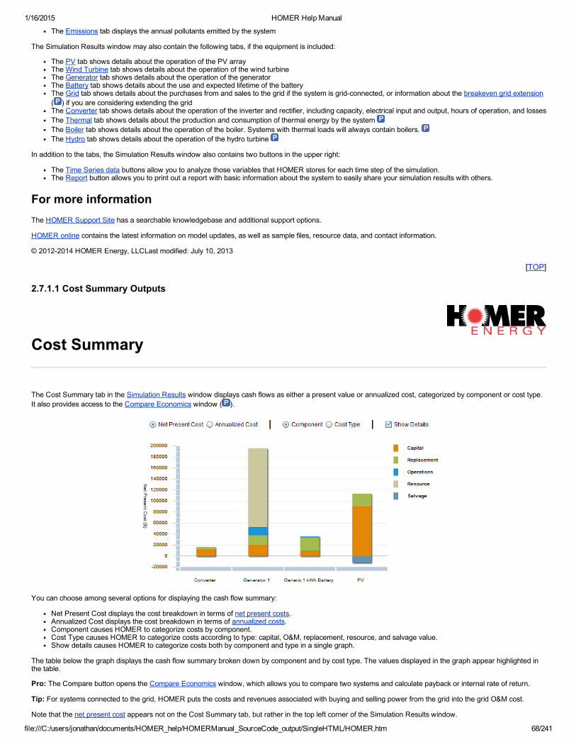
1/16/2015 HOMER Help Manual
file:///C:/users/jonathan/documents/HOMER_help/HOMERManual_SourceCode_output/SingleHTML/HOMER.htm 68/241
The Emissions tab displays the annual pollutants emitted by the system
The Simulation Results window may also contain the following tabs, if the equipment is included:
The PV tab shows details about the operation of the PV arrayThe Wind Turbine tab shows details about the operation of the wind turbineThe Generator tab shows details about the operation of the generatorThe Battery tab shows details about the use and expected lifetime of the batteryThe Grid tab shows details about the purchases from and sales to the grid if the system is gridconnected, or information about the breakeven grid extension( ) if you are considering extending the gridThe Converter tab shows details about the operation of the inverter and rectifier, including capacity, electrical input and output, hours of operation, and lossesThe Thermal tab shows details about the production and consumption of thermal energy by the system The Boiler tab shows details about the operation of the boiler. Systems with thermal loads will always contain boilers. The Hydro tab shows details about the operation of the hydro turbine
In addition to the tabs, the Simulation Results window also contains two buttons in the upper right:
The Time Series data buttons allow you to analyze those variables that HOMER stores for each time step of the simulation.The Report button allows you to print out a report with basic information about the system to easily share your simulation results with others.
For more informationThe HOMER Support Site has a searchable knowledgebase and additional support options.
HOMER online contains the latest information on model updates, as well as sample files, resource data, and contact information.
© 20122014 HOMER Energy, LLCLast modified: July 10, 2013
[TOP]
2.7.1.1 Cost Summary Outputs
Cost Summary
The Cost Summary tab in the Simulation Results window displays cash flows as either a present value or annualized cost, categorized by component or cost type.It also provides access to the Compare Economics window ( ).
You can choose among several options for displaying the cash flow summary:
Net Present Cost displays the cost breakdown in terms of net present costs.Annualized Cost displays the cost breakdown in terms of annualized costs.Component causes HOMER to categorize costs by component.Cost Type causes HOMER to categorize costs according to type: capital, O&M, replacement, resource, and salvage value.Show details causes HOMER to categorize costs both by component and type in a single graph.
The table below the graph displays the cash flow summary broken down by component and by cost type. The values displayed in the graph appear highlighted inthe table.
Pro: The Compare button opens the Compare Economics window, which allows you to compare two systems and calculate payback or internal rate of return.
Tip: For systems connected to the grid, HOMER puts the costs and revenues associated with buying and selling power from the grid into the grid O&M cost.
Note that the net present cost appears not on the Cost Summary tab, but rather in the top left corner of the Simulation Results window.

1/16/2015 HOMER Help Manual
file:///C:/users/jonathan/documents/HOMER_help/HOMERManual_SourceCode_output/SingleHTML/HOMER.htm 69/241
See also
Simulation Results window
Cash Flow tab
Compare Economics window
Net present cost
Annualized cost
For more informationThe HOMER Support Site has a searchable knowledgebase and additional support options.
HOMER online contains the latest information on model updates, as well as sample files, resource data, and contact information.
© 20122014 HOMER Energy, LLCLast modified: Sept 28, 2012
[TOP]
2.7.1.1.1 Compare Economics Window
Compare Economics Window
This window allows you to compare the economic merits of the current system and a base case system. The window displays cash flow graphs and a table ofeconomic metrics. To open the window, choose a system to be the current system in optimization results, and then click Compare on the Cost Summary page ofthe Simulation Results window.
You must choose a base case system to compare with the current system to make the economic metrics meaningful. The metrics show you the value of thedifference between two options, taking into account the lifecycle costs of both systems. You can compare the current system to any other system in the optimizationresults. For example:
Compare a PVwinddiesel hybrid system with a dieselonly base case system for an offgrid project to find the present worth of fuel saved by installing ahybrid system instead of a dieselonly system, taking into account the cost of installing, operating, and maintaining each system.Compare a gridconnected PV system to a gridonly system to find the payback period required for grid sales to recover the cost of installing the PV system.
The table at the top of the window displays a list of systems from the optimization results from which you can choose a base case. You can display the list as acategorized list to display only the topranked system in each category, or as an overall list to display all systems.
The system summary table shows the component sizes, capital cost and net present cost of the base case system and current system.
The display options control what appears in the cash flow graph.
Tip: Rightclick the cash flow graph to export a table of values to a text file, which you can open in a text editor or spreadsheet program.
When you choose a base case system, the metric table shows economic measures representing the value of the difference between the two systems:
The present worth is the difference between the net present costs of the base case system and the current system. The sign of the present worth indicateswhether the current system compares favorably as an investment option with the base case system: A positive value indicates that the current system savesmoney over the project lifetime compared to the base case system.The annual worth is the present worth multiplied by the capital recovery factor.To see how HOMER calculates return on investment (ROI), choose the following display options: Graph, Difference, Cumulative. Subtract the cumulativenominal cash flow in year zero from the cumulative nominal cash flow in the final year. Divide that number by the lifetime and then again by the cumulativenominal cash flow in year zero. Note that the cumulative nominal cash flow in year zero is equivalent to the base case capital cost minus the current systemcapital cost.Internal rate of return (IRR) is the discount rate at which the base case and current system have the same net present cost. HOMER calculates the IRR bydetermining the discount rate that makes the present value of the difference of the two cash flow sequences equal to zero.Payback is the number of years at which the cumulative cash flow of the difference between the current system and base case system switches fromnegative to positive. The payback is an indication of how long it would take to recover the difference in investment costs between the current system and thebase case system. You can see a visual representation of the payback by choosing the following display options: Graph, Difference, and Cumulative. Thesimple payback is where the nominal cash flow difference line crosses zero. The discounted payback is where the discounted cash flow difference linecrosses zero.
See also
Why does HOMER require a base case to calculate payback and other economic metrics?
Is there a way to calculate simple payback by hand?
For more informationThe HOMER Support Site has a searchable knowledgebase and additional support options.
HOMER online contains the latest information on model updates, as well as sample files, resource data, and contact information.

1/16/2015 HOMER Help Manual
file:///C:/users/jonathan/documents/HOMER_help/HOMERManual_SourceCode_output/SingleHTML/HOMER.htm 70/241
© 20122014 HOMER Energy, LLCLast modified: June 6, 2008
[TOP]
2.7.1.1.2 Calculating Payback, Internal Rate of Return (IRR) and Other Economic Metrics
Calculating payback
HOMER calculates payback by comparing one system with another. In general, payback tells you how many years it will take to recover an investment. You investa certain amount of money up front, then earn income from that investment, and the payback is the number of years it takes for the cumulative income to equal thevalue of the initial investment. HOMER can also calculate other economic metrics such as IRR, present worth, and return on investment.
Sometimes, the "income" of a power system can be defined intrinsically, without a reference for comparison. If, for example, a gridsales system does not need toserve any load, but simply sells power to the grid, then you can define the income of the system as the money it makes by selling power to the grid minus theexpense of operating the system. In that case, you could compare the initial cost of the system with its income to calculate the payback.
For distributed power systems, it's usually not that simple, and the income must be defined relative to some alternative. Say you are designing a system to provideelectricity to an offgrid house. A pure diesel system might have low capital cost and high operating cost, whereas a PVdieselbattery system might have highcapital cost and low operating cost. Neither system produces any income. In both cases you spend money up front to build the system, then you keep spendingmoney each year to operate the system. The concept of payback has meaning only if you compare one system to the other. You can define the payback of theadditional investment required for the PVdieselbattery system by comparing the difference in capital cost with the difference in operating cost. HOMER doesexactly that in the Compare Economics window.
So, to calculate the payback of one alternative, we must compare to another alternative. Even to calculate the payback of the simple gridsales system mentionedabove involves an implicit comparison with the base case, which is to do nothing. The donothing alternative is easy to compare to, since all its costs are zero, but ifwe have an electric load to serve, the donothing alternative is not an acceptable one.
A renewable power system designer will often use a nonrenewable power system as the base case, but HOMER lets you choose any base case you want. Youcould compare a system with two wind turbines to a system that has one wind turbine to calculate the payback of the second wind turbine. Or you could compare aPVdieselbattery system with a PVdiesel system to calculate the payback of the battery.
See also:
Compare Economics window
Is there a way to calculate simple payback by hand?
For more informationThe HOMER Support Site has a searchable knowledgebase and additional support options.
HOMER online contains the latest information on model updates, as well as sample files, resource data, and contact information.
© 20122014 HOMER Energy, LLCLast modified: Sept 28, 2012
[TOP]
2.7.1.1.3 Grid Costs
Grid Costs
Since the grid is unlike any other component, HOMER calculates the costs associated with the grid in a unique way. This article explains how HOMER calculateseach of the grid cost outputs.
Grid capital costIf the system is connected to the grid and contains some other power producing device (such as a microturbine, a fuel cell, a PV array, or a wind turbine), the gridcapital cost is equal to the interconnection charge. Otherwise, the grid capital cost is zero.
Grid replacement costThe replacement cost of the grid is always zero.
Grid O&M costThe grid O&M cost is equal to the annual cost of buying electricity from the grid (energy cost plus demand cost) minus any income from the sale of electricity to thegrid. For gridconnected systems that contain some other power producing device (such as a microturbine, a fuel cell, a PV array, or a wind turbine), the grid O&M
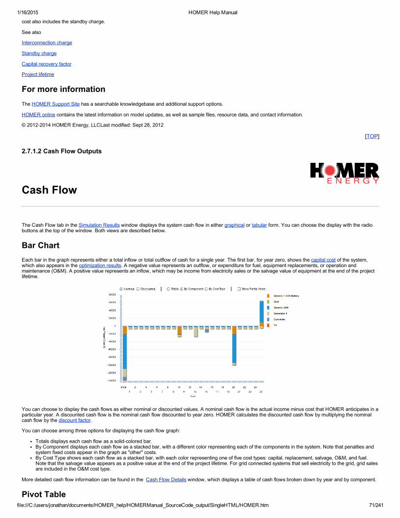
1/16/2015 HOMER Help Manual
file:///C:/users/jonathan/documents/HOMER_help/HOMERManual_SourceCode_output/SingleHTML/HOMER.htm 71/241
cost also includes the standby charge.
See also
Interconnection charge
Standby charge
Capital recovery factor
Project lifetime
For more informationThe HOMER Support Site has a searchable knowledgebase and additional support options.
HOMER online contains the latest information on model updates, as well as sample files, resource data, and contact information.
© 20122014 HOMER Energy, LLCLast modified: Sept 28, 2012
[TOP]
2.7.1.2 Cash Flow Outputs
Cash Flow
The Cash Flow tab in the Simulation Results window displays the system cash flow in either graphical or tabular form. You can choose the display with the radiobuttons at the top of the window. Both views are described below.
Bar ChartEach bar in the graph represents either a total inflow or total outflow of cash for a single year. The first bar, for year zero, shows the capital cost of the system,which also appears in the optimization results. A negative value represents an outflow, or expenditure for fuel, equipment replacements, or operation andmaintenance (O&M). A positive value represents an inflow, which may be income from electricity sales or the salvage value of equipment at the end of the projectlifetime.
You can choose to display the cash flows as either nominal or discounted values. A nominal cash flow is the actual income minus cost that HOMER anticipates in aparticular year. A discounted cash flow is the nominal cash flow discounted to year zero. HOMER calculates the discounted cash flow by multiplying the nominalcash flow by the discount factor.
You can choose among three options for displaying the cash flow graph:
Totals displays each cash flow as a solidcolored bar.By Component displays each cash flow as a stacked bar, with a different color representing each of the components in the system. Note that penalties andsystem fixed costs appear in the graph as "other" costs.By Cost Type shows each cash flow as a stacked bar, with each color representing one of five cost types: capital, replacement, salvage, O&M, and fuel.Note that the salvage value appears as a positive value at the end of the project lifetime. For grid connected systems that sell electricity to the grid, grid salesare included in the O&M cost type.
More detailed cash flow information can be found in the Cash Flow Details window, which displays a table of cash flows broken down by year and by component.
Pivot Table

1/16/2015 HOMER Help Manual
file:///C:/users/jonathan/documents/HOMER_help/HOMERManual_SourceCode_output/SingleHTML/HOMER.htm 72/241
Choose "Pivot Table" from the radio buttons at the top of the cash flow window. The cash flow details table shows a detailed breakdown of all the costs that occurthroughout the project lifetime. It appears in the Cash Flow Details window.
An example of the cash flow details table appears below. Each year of the project lifetime appears as a column. The rows list the capital cost, replacement cost,salvage value, O&M cost, fuel cost, and total cost for each component. Nominal costs appear in the top half of the table, and discounted costs appear in the bottomhalf. The discount factors, which HOMER uses to calculate discounted costs from nominal costs, appear in between.
Tip: Using the controls at the top of the window, you can choose to display a lessdetailed breakdown of the costs, or to display only nominal or only discountedcosts.
The example above shows the cash flows for a system comprised of a diesel generator and a wind turbine. The project lifetime is ten years. The diesel generatorneeds to be replaced at a cost of $5,500 every two years, and the wind turbine needs to be replaced at a cost of $12,000 every eight years.
Capital CostsCapital costs occur only at the beginning of the project, meaning at the end of year zero. No capital costs occur after year zero.
Replacement CostsReplacements costs occur whenever a component needs a replacement. Note that replacement costs may not necessarily occur at integer year numbers. Forexample, if a generator requires replacement every 3.25 years, HOMER will assign replacement costs at 3.25 years, 6.5 years, and so on. Use the controls at thetop of the window if you want to see the precise timing of these cash flows.
Salvage ValueSalvage value occurs as a positive cash flow at the end of the project lifetime, for any component that has some remaining life at this point. In the example above,the wind turbine requires replacement after eight years, so the second wind turbine is only two years old at the end of the tenyear project lifetime, meaning it hassix years remaining in its lifetime. HOMER assumes linear depreciation, so it calculates a salvage value of 6/8 = 75% of the replacement cost of the wind turbine.Since the wind turbine replacement cost is $12,000, that leads to a salvage value of $9,000 for the wind turbine at the end of the project lifetime.
Operating and Maintenance CostsFor many components, such as the PV array and the wind turbine, you enter the O&M costs in dollars per year. For other components, such as the generator, youenter the O&M cost in dollars per operating hour, and HOMER multiplies that number by the operating hours per year to calculate the resulting annual O&M cost indollars per year. Note that the number HOMER reports for the grid O&M cost is actually the annual cost of buying power from the grid minus the annual revenuegained from sales of power to the grid.
Fuel CostsFor components that consume fuel, HOMER calculates the annual fuel cost by multiplying the fuel price by the annual fuel consumption.
Tip: The bottom row of the table, when displaying discounted costs, shows the total discounted cost for each year of the project lifetime. The sum of thesenumbers, which appears in the bottom right corner of the table, equals the total net present cost of the system.
See also
Simulation Results window
Cost Summary tab
Cash Flow Details window
Discount factor

1/16/2015 HOMER Help Manual
file:///C:/users/jonathan/documents/HOMER_help/HOMERManual_SourceCode_output/SingleHTML/HOMER.htm 73/241
For more informationThe HOMER Support Site has a searchable knowledgebase and additional support options.
HOMER online contains the latest information on model updates, as well as sample files, resource data, and contact information.
© 20122014 HOMER Energy, LLCLast modified: July 9, 2013
[TOP]
2.7.1.3 Electrical Outputs
Electrical Outputs
The Electrical tab in the Simulation Results window shows details about the annual production and consumption of electrical energy by the system.
ProductionThis table lists the total annual energy output of each electrical energy producing component of the power system, plus the total electrical production.
ConsumptionThis table lists the total amount of electrical energy that went to serve each of the system's electrical loads. Values that appear here when applicable include:
Variable DescriptionAC Primary Load Served The amount of energy that went towards serving the AC primary load(s)
DC Primary Load Served The amount of energy that went towards serving the DC primary load(s)
Deferrable Load Served The amount of energy that went towards serving the deferrable load
Electrolyzer Load Served The amount of electrical energy consumed by the electrolyzer
Grid Sales The total amount of electricity sold to the grid during the year
Total Load Served The total amount of electrical load served during the year
Note: The total production can exceed the sum of the total consumption and the excess electricity because of losses in the battery and converter.
Excess and ShortageThis table lists the following values:
Variable DescriptionExcessElectricity
The total amount of excess electricity that occurred during the year, as well as the excess electricity fraction expressed as apercentage of the total electrical production
UnmetElectricLoad
The total amount of unmet load that that went unserved because of insufficient generation during the year, as well as the unmetload fraction expressed as a percentage of the total electrical demand
CapacityShortage
The total amount of capacity shortage that occurred during the year, as well as the capacity shortage fraction expressed as apercentage of the total electrical demand
Other OutputsThe final table lists the following variables:
Variable DescriptionRenewable Fraction The fraction of the total electrical production that is produced by renewable sources
Maximum Renewable Penetration The maximum value of the renewable penetration that occurs over the year
See also
Simulation Results window

1/16/2015 HOMER Help Manual
file:///C:/users/jonathan/documents/HOMER_help/HOMERManual_SourceCode_output/SingleHTML/HOMER.htm 74/241
Constraints window
Written by: Tom Lambert ([email protected])Last modified: September 27, 2010
For more informationThe HOMER Support Site has a searchable knowledgebase and additional support options.
HOMER online contains the latest information on model updates, as well as sample files, resource data, and contact information.
© 20122014 HOMER Energy, LLCLast modified: July 1, 2013
[TOP]
2.7.1.4 PV Outputs
PV Outputs
The PV tab in the Simulation Results window contains the following output variables:
Variable DescriptionRated Capacity The rated capacity of the PV array under standard conditions, in kW
Mean Output The average power amount of the PV array over the year, in kW and kWh/day
Capacity Factor The average power output of the PV array (in kW) divided by its rated power, in %
Total Production The total power output of the PV array over the year, in kWh/yr
Minimum Output The minimum power output of the PV array over the year, in kW
Maximum Output The maximum power output of the PV array over the year, in kW
PV Penetration The average power output of the PV array divided by the average primary load, in %
Hours of Operation The number of hours of the year during which the PV array output was greater than zero
Levelized Cost The levelized cost of energy of the PV array, in $/kWh
In the bottom half of the page a DMap appears showing the power output of the PV array in each time step of the year.
Written by: Tom Lambert ([email protected])Last modified: October 27, 2004
For more informationThe HOMER Support Site has a searchable knowledgebase and additional support options.
HOMER online contains the latest information on model updates, as well as sample files, resource data, and contact information.
© 20122014 HOMER Energy, LLCLast modified: July 1, 2013
[TOP]
2.7.1.5 Wind Turbine Outputs
Wind Turbine Outputs
The Wind Turbine tab in the Simulation Results window contains the following output variables:
Variable DescriptionTotal Rated Capacity The highest possible power amount from the wind turbine(s), in kW

1/16/2015 HOMER Help Manual
file:///C:/users/jonathan/documents/HOMER_help/HOMERManual_SourceCode_output/SingleHTML/HOMER.htm 75/241
Mean Output The average power amount of the wind turbine over the year, in kWCapacity Factor The average power output of the wind turbine(s) divided by the total wind turbine capacity, in %
Total Production The total power output of the wind turbine(s) over the year, in kWh/yr
Minimum Output The minimum power output of the wind turbine over the year, in kW
Maximum Output The maximum power output of the wind turbine over the year, in kW
Wind Penetration The average power output of the wind turbine(s) divided by the average primary load, in %
Hours of Operation The number of hours of the year during which the wind turbine output was greater than zero
Levelized Cost The levelized cost of energy of the wind turbine(s), in $/kWh
In the bottom half of the page a DMap appears showing the power output of the wind turbine(s) in each time step of the year.
Written by: Tom Lambert ([email protected])Last modified: October 27, 2004
For more informationThe HOMER Support Site has a searchable knowledgebase and additional support options.
HOMER online contains the latest information on model updates, as well as sample files, resource data, and contact information.
© 20122014 HOMER Energy, LLCLast modified: July 1, 2013
[TOP]
2.7.1.6 Generator Outputs
Generator Outputs
The Generator tab in the Simulation Results window contains the following output variables:
Variable DescriptionHours of Operation The total run time of the generator during the year, in hr/yr
Number of Starts The number of times the generator was started during the year
Operational Life The number of years the generator will last before it requires replacement
Capacity Factor The average power output of the generator divided by its total capacity
Fixed Generation Cost The fixed cost of running the generator, in $/hr
Electrical Production The total power output of the generator over the year, in kWh/yr
Mean Electrical Output The average electrical power output of the generator over the hours that it runs, in kW
Minimum Electrical Output The lowest electrical power output of the generator over the year, in kW
Maximum Electrical Output The highest electrical power output of the generator over the year, in kW
Average Thermal Output The average thermal power output of the generator over the hours that it runs
Minimum Thermal Output The lowest thermal power output of the generator over the year
Maximum Thermal Output The highest thermal power output of the generator over the year
Fuel Consumption The total amount of fuel consumed by the generator during the year, in L/yr
Specific Fuel Consumption The average quantity of fuel consumed per kWh of energy produced by the generator, in L/kWh
Fuel Energy Input The total amount of energy in the fuel consumed by the generator during the year in kWh/yr
Mean Electrical Efficiency The average electrical efficiency of the generator during the year, in %
Note : The thermal output variables appear only if the heat recovery ratio is nonzero.
In the bottom half of the page a DMap appears showing the power output of the generator in each hour of the year.
Written by: Tom Lambert ([email protected])Last modified: October 27, 2004
1/16/2015 HOMER Help Manual
file:///C:/users/jonathan/documents/HOMER_help/HOMERManual_SourceCode_output/SingleHTML/HOMER.htm 76/241
For more informationThe HOMER Support Site has a searchable knowledgebase and additional support options.
HOMER online contains the latest information on model updates, as well as sample files, resource data, and contact information.
© 20122014 HOMER Energy, LLCLast modified: July 1, 2013
[TOP]
2.7.1.7 Battery Outputs
Battery Outputs
The Battery tab in the Simulation Results window contains the following output variables:
Variable DescriptionString Size The number of batteries connected in series in each string
Strings in Parallel The number of battery strings connected in parallel
Batteries The number of batteries in the array is the string size multiplied by the number of strings
Bus Voltage The voltage of the battery array, calculated by multiplying battery voltage by string size, in volts
Nominal Capacity The amount of energy that could be withdrawn from the battery at a particular constant current, starting from a fullycharged state, in kWh
Usable NominalCapacity The battery capacity adjusted to exclude all capacity below the minimum state of charge of the battery, in kWh
Autonomy The capacity of the battery bank divided by the average electrical load, in hours
Lifetime Throughput The total amount of energy that can be cycled through the battery before it needs to be replaced, in kWh
Battery Wear Cost The cost of cycling energy through the battery bank, in $/kWh
Average Energy Cost The average cost of the energy that goes into the battery, in $/kWh
Energy In The total amount of energy charged to the battery, in kWh
Energy Out The total amount of energy discharged from the battery, in kWh
Storage Depletion The difference in the battery state of charge at the beginning and end of the year, in kWh/yr
Losses Annual energy losses due to battery inefficiency, in kWh/yr
Annual Throughput The total amount of energy that cycled through the battery bank during the year, in kWh/yr
Expected Life The number of years the battery bank will last before it requires replacement
In the bottom half of the page a DMap appears showing the state of charge of the battery bank in each time step of the year.
For more informationThe HOMER Support Site has a searchable knowledgebase and additional support options.
HOMER online contains the latest information on model updates, as well as sample files, resource data, and contact information.
© 20122014 HOMER Energy, LLCLast modified: July 1, 2013
[TOP]
2.7.1.8 Grid Outputs
Grid Outputs
The Grid tab in the Simulation Results window displays details about the buying and selling of electricity from and to the grid, and the resulting costs. The outputstable contains the following variables:
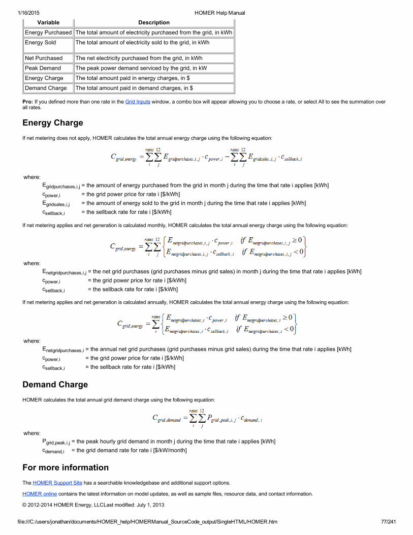
1/16/2015 HOMER Help Manual
file:///C:/users/jonathan/documents/HOMER_help/HOMERManual_SourceCode_output/SingleHTML/HOMER.htm 77/241
Variable DescriptionEnergy Purchased The total amount of electricity purchased from the grid, in kWh
Energy Sold The total amount of electricity sold to the grid, in kWh
Net Purchased The net electricity purchased from the grid, in kWh
Peak Demand The peak power demand serviced by the grid, in kW
Energy Charge The total amount paid in energy charges, in $
Demand Charge The total amount paid in demand charges, in $
Pro: If you defined more than one rate in the Grid Inputs window, a combo box will appear allowing you to choose a rate, or select All to see the summation overall rates.
Energy ChargeIf net metering does not apply, HOMER calculates the total annual energy charge using the following equation:
where:Egridpurchases,i,j = the amount of energy purchased from the grid in month j during the time that rate i applies [kWh]cpower,i = the grid power price for rate i [$/kWh]Egridsales,i,j = the amount of energy sold to the grid in month j during the time that rate i applies [kWh]csellback,i = the sellback rate for rate i [$/kWh]
If net metering applies and net generation is calculated monthly, HOMER calculates the total annual energy charge using the following equation:
where:Enetgridpurchases,i,j = the net grid purchases (grid purchases minus grid sales) in month j during the time that rate i applies [kWh]cpower,i = the grid power price for rate i [$/kWh]csellback,i = the sellback rate for rate i [$/kWh]
If net metering applies and net generation is calculated annually, HOMER calculates the total annual energy charge using the following equation:
where:Enetgridpurchases,i = the annual net grid purchases (grid purchases minus grid sales) during the time that rate i applies [kWh]cpower,i = the grid power price for rate i [$/kWh]csellback,i = the sellback rate for rate i [$/kWh]
Demand ChargeHOMER calculates the total annual grid demand charge using the following equation:
where:Pgrid,peak,i,j = the peak hourly grid demand in month j during the time that rate i applies [kWh]cdemand,i = the grid demand rate for rate i [$/kW/month]
For more informationThe HOMER Support Site has a searchable knowledgebase and additional support options.
HOMER online contains the latest information on model updates, as well as sample files, resource data, and contact information.
© 20122014 HOMER Energy, LLCLast modified: July 1, 2013

1/16/2015 HOMER Help Manual
file:///C:/users/jonathan/documents/HOMER_help/HOMERManual_SourceCode_output/SingleHTML/HOMER.htm 78/241
[TOP]
2.7.1.9 Converter Outputs
Converter Outputs
The Converter tab in the Simulation Results window displays the following variables for both the inverter, which converts DC to AC electricity, and the rectifier,which converts AC to DC electricity:
Variable DescriptionCapacity The maximum possible power output, in AC kW for the inverter and DC kW for the rectifier
Mean, Min and Max Output The inverter values are in terms of AC kW, and the rectifier values are in terms of DC kW
Capacity Factor The mean output divided by the capacity, in %
Hours of Operation The number of hours of nonzero power output
Energy In The total amount of energy into the device, in DC kWh/yr for the inverter and AC kWh/yr for the rectifier
Energy Out The total amount of energy out of the device, in AC kWh for the inverter and DC kWh for the rectifier
Losses The total energy lost in the device, in kWh/yr
In the bottom half of the page a DMap appears showing the power output of the inverter and/or rectifier in each time step of the year.
For more informationThe HOMER Support Site has a searchable knowledgebase and additional support options.
HOMER online contains the latest information on model updates, as well as sample files, resource data, and contact information.
© 20122014 HOMER Energy, LLCLast modified: July 1, 2013
[TOP]
2.7.1.10 Emissions Outputs
Emissions Outputs
The Emissions tab in the Simulation Results window shows the total amount of each pollutant produced annually by the power system in kg/yr. Pollutants originatefrom the consumption of fuel and biomass in generators, the boiler, and the reformer, as well as from the consumption of grid power.
Sales of power to the grid result in reduced grid emissions, and HOMER credits the power system with these reductions. The system can even achieve negativeemissions of one or more pollutants if it sells a lot of lowemissions electricity to the grid.
See also
How HOMER calculates emissions
Written by: Tom Lambert ([email protected])Last modified: October 27, 2004
For more informationThe HOMER Support Site has a searchable knowledgebase and additional support options.
HOMER online contains the latest information on model updates, as well as sample files, resource data, and contact information.
© 20122014 HOMER Energy, LLCLast modified: July 11, 2013
[TOP]
2.7.1.11 Thermal Outputs

1/16/2015 HOMER Help Manual
file:///C:/users/jonathan/documents/HOMER_help/HOMERManual_SourceCode_output/SingleHTML/HOMER.htm 79/241
Thermal Outputs
This feature requires the Combined Heat and Power Module.
Click for more information.
The Thermal tab in the Simulation Results window shows details about the annual production and consumption of thermal energy by the system.
Annual Thermal Energy ProductionThis section lists the total annual output of each thermal energy producing component of the power system, as well as the total thermal production.
Annual Thermal Load ServedThis section shows the total total thermal load served over the year, plus any surplus.
For more informationThe HOMER Support Site has a searchable knowledgebase and additional support options.
HOMER online contains the latest information on model updates, as well as sample files, resource data, and contact information.
© 20122014 HOMER Energy, LLCLast modified: Sept 28, 2012
[TOP]
2.7.1.12 Boiler Outputs
Boiler Outputs
This feature requires the Combined Heat and Power Module.
Click for more information.
The Boiler tab in the Simulation Results window contains the following output variables:
Variable DescriptionHours of Operation The total run time of the boiler during the year, in hr/yr
Total Production The total amount of thermal energy produced by the boiler per year, in kWh/yr
Mean Output The average thermal power output of the boiler over the hours that it runs, in kW
Min. Output The lowest thermal power output of the boiler over the year, in kW
Max. Output The highest thermal power output of the boiler over the year, in kW
Fuel Consumption The total amount of fuel consumed by the boiler during the year, in L/yr
Specific Fuel Consumption The average quantity of fuel consumed per kWh of thermal energy produced by the boiler, in L/kWh
Mean Efficiency The total annual thermal energy production divided by the total annual fuel energy consumption, in %
In the bottom half of the page a DMap appears showing the thermal power output of the boiler in each time step of the year.
Written by: Tom Lambert ([email protected])Last modified: January 21, 2010
For more informationThe HOMER Support Site has a searchable knowledgebase and additional support options.
HOMER online contains the latest information on model updates, as well as sample files, resource data, and contact information.
© 20122014 HOMER Energy, LLCLast modified: Sept 28, 2012
[TOP]

1/16/2015 HOMER Help Manual
file:///C:/users/jonathan/documents/HOMER_help/HOMERManual_SourceCode_output/SingleHTML/HOMER.htm 80/241
2.7.1.13 Hydro Outputs
Hydro Outputs
This feature requires the Hydro Module.
Click for more information.
The Hydro tab in the Simulation Results window contains the following output variables:
Variable DescriptionAverage Output The average power amount of the hydro turbine over the year, in kW
Minimum Output The minimum power output of the hydro turbine over the year, in kW
Maximum Output The maximum power output of the hydro turbine over the year, in kW
Hydro Penetration The average power output of the hydro turbine divided by the average primary load
Capacity Factor The average power output of the hydro turbine divided by its nominal capacity
Hours of Operation The number of hours of the year during which the hydro turbine output was greater than zero
In the bottom half of the page a DMap appears showing the power output of the hydro turbine in each time step of the year.
Written by: Tom Lambert ([email protected])Last modified: October 27, 2004
For more informationThe HOMER Support Site has a searchable knowledgebase and additional support options.
HOMER online contains the latest information on model updates, as well as sample files, resource data, and contact information.
© 20122014 HOMER Energy, LLCLast modified: July 12, 2013
[TOP]
2.7.1.14 Time Series Outputs
Time series outputs
PlotThe time series plot can graph a number of model variables over the duration of the simulation.
Scatterplot The scatterplot graph allows you to plot any variable against any other variable. This kind of graph can often help you to understand how the system operates. Forexample, plotting diesel power output versus battery state of charge may reveal that the diesel only operates when the battery is at or near its minimum state ofcharge.
DeltaplotThe deltaplot shows the frequency of changes in any variable over some length of time. Choose the variable from the dropdown box, and choose the length oftime using the slider control.
TableThe table displays all of the time series data generated by the simulation for each time step.
Export

1/16/2015 HOMER Help Manual
file:///C:/users/jonathan/documents/HOMER_help/HOMERManual_SourceCode_output/SingleHTML/HOMER.htm 81/241
The export function writes all time series data from the selected simulation to a csv file. You will be prompted for a location and name for the output file.
For more informationThe HOMER Support Site has a searchable knowledgebase and additional support options.
HOMER online contains the latest information on model updates, as well as sample files, resource data, and contact information.
© 2012 HOMER Energy, LLCLast modified: January 21, 2010
[TOP]
2.7.1.15 Hydrogen Outputs
Hydrogen Outputs
The Hydrogen tab in the Simulation Results window contains the following output variables:
Variable DescriptionElectrolyzer Production The total amount of hydrogen produced by the electrolyzer, in kg/yr
Reformer Production The total amount of hydrogen produced by the reformer, in kg/yr
Total Hydrogen Production The total amount of hydrogen produced by the system, in kg/yr
Unmet Hydrogen Load The total hydrogen demand that the system was unable to supply, in kg/yr
Electrolyzer Capacity Factor The average production of the electrolyzer divided by its rated production capacity
Reformer Capacity Factor The average production of the reformer divided by its rated production capacity
Written by: Tom Lambert ([email protected])Last modified: October 27, 2004
For more informationThe HOMER Support Site has a searchable knowledgebase and additional support options.
HOMER online contains the latest information on model updates, as well as sample files, resource data, and contact information.
© 20122014 HOMER Energy, LLCLast modified: Sept 28, 2012
[TOP]
2.7.1.16 Hydrogen Tank Outputs
Hydrogen Tank Outputs
The Hydrogen Tank tab in the Simulation Results window contains the following output variables:
Variable DescriptionHydrogen Production The total amount of hydrogen produced annually by the system
Hydrogen Consumption The total amount of hydrogen consumed annually by the system
Hydrogen Tank Autonomy The energy capacity of the hydrogen tank divided by the average electrical load
This page also contains three graphs showing the amount of hydrogen in the tank over the year.
For more informationThe HOMER Support Site has a searchable knowledgebase and additional support options.

1/16/2015 HOMER Help Manual
file:///C:/users/jonathan/documents/HOMER_help/HOMERManual_SourceCode_output/SingleHTML/HOMER.htm 82/241
HOMER online contains the latest information on model updates, as well as sample files, resource data, and contact information.
© 20122014 HOMER Energy, LLCLast modified: June 21, 2004
[TOP]
2.7.1.17 Electrolyzer Outputs
Electrolyzer Outputs
The Electrolyzer tab in the Simulation Results window contains the following output variables:
Variable DescriptionRated Capacity The maximum electrical input power the electrolyzer can accept
Mean Input The average electrical input power to the electrolyzer over the year
Minimum Input The minimum electrical input power to the electrolyzer over the year
Maximum Input The maximum electrical input power to the electrolyzer over the year
Total Input Energy The total electrical energy that the electrolyzer consumes annually
Capacity Factor The mean input power divided by the rated capacity
Hours of Operation The number of hours per year that the electrolyzer produces hydrogen
Mean Output The average rate of hydrogen production over the year
Minimum Output The minimum rate of hydrogen production over the year
Maximum Output The maximum rate of hydrogen production over the year
Total Production The total amount of hydrogen produced annually by the electrolyzer
Specific Consumption The average quantity of fuel consumed per kWh of thermal energy produced by the electrolyzer
In the bottom half of the page a DMap appears showing the electrical power consumption of the electrolyzer in each time step of the year.
Written by: Tom Lambert ([email protected])Last modified: January 22, 2010
For more informationThe HOMER Support Site has a searchable knowledgebase and additional support options.
HOMER online contains the latest information on model updates, as well as sample files, resource data, and contact information.
© 20122014 HOMER Energy, LLCLast modified: Sept 28, 2012
[TOP]
2.7.1.18 Report Summarizing the Simulation Results
Report Summarizing the Simulation Results
To view a report summarizing the results of a simulation, click the Report button in the bottom left corner of the Simulation Results window:
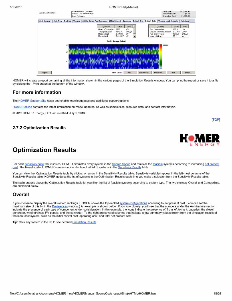
1/16/2015 HOMER Help Manual
file:///C:/users/jonathan/documents/HOMER_help/HOMERManual_SourceCode_output/SingleHTML/HOMER.htm 83/241
HOMER will create a report containing all the information shown in the various pages of the Simulation Results window. You can print the report or save it to a fileby clicking the Print button at the bottom of the window.
For more informationThe HOMER Support Site has a searchable knowledgebase and additional support options.
HOMER online contains the latest information on model updates, as well as sample files, resource data, and contact information.
© 2012 HOMER Energy, LLCLast modified: July 1, 2013
[TOP]
2.7.2 Optimization Results
Optimization Results
For each sensitivity case that it solves, HOMER simulates every system in the Search Space and ranks all the feasible systems according to increasing net presentcost. The Results tab of HOMER's main window displays that list of systems in the Sensitivity Results table.
You can view the Optimization Results table by clicking on a row in the Sensitivity Results table. Sensitivity variables appear in the leftmost columns of theSensitivity Results table. HOMER updates the list of systems in the Optimization Results each time you make a selection from the Sensitivity Results table.
The radio buttons above the Optimization Results table let you filter the list of feasible systems according to system type. The two choices, Overall and Categorized,are explained below.
OverallIf you choose to display the overall system rankings, HOMER shows the topranked system configurations according to net present cost. (You can set themaximum size of this list in the Preferences window.) An example is shown below. If you look closely, you'll see that the numbers under the Architecture sectionindicate the presence of each type of component under consideration. In this example, the icons indicate the presence of, from left to right: batteries, the dieselgenerator, wind turbines, PV panels, and the converter. To the right are several columns that indicate a few summary values drawn from the simulation results ofthe leastcost system, such as the initial capital cost, operating cost, and total net present cost.
Tip: Click any system in the list to see detailed Simulation Results.
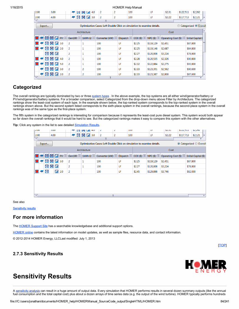
1/16/2015 HOMER Help Manual
file:///C:/users/jonathan/documents/HOMER_help/HOMERManual_SourceCode_output/SingleHTML/HOMER.htm 84/241
CategorizedThe overall rankings are typically dominated by two or three system types . In the above example, the top systems are all either wind/generator/battery orPV/wind/generator/battery systems. For a broader comparison, select Categorized from the dropdown menu above Filter by Architecture. The categorizedrankings show the leastcost system of each type. In the example shown below, the topranked system corresponds to the topranked system in the overallrankings shown above. But the second system listed corresponds to the sixthplace system in the overall rankings, because the secondplace system in the overallrankings was of the same type as the firstplace system.
The fifth system in the categorized rankings is interesting for comparison because it represents the leastcost pure diesel system. This system would both appearso far down the overall rankings that it would be hard to see. But the categorized rankings makes it easy to compare this system with the other alternatives.
Tip: Click any system in the list to see detailed Simulation Results.
See also
Sensitivity results
For more informationThe HOMER Support Site has a searchable knowledgebase and additional support options.
HOMER online contains the latest information on model updates, as well as sample files, resource data, and contact information.
© 20122014 HOMER Energy, LLCLast modified: July 1, 2013
[TOP]
2.7.3 Sensitivity Results
Sensitivity Results
A sensitivity analysis can result in a huge amount of output data. Every simulation that HOMER performs results in several dozen summary outputs (like the annualfuel consumption and the total capital cost) plus about a dozen arrays of time series data (e.g. the output of the wind turbine). HOMER typically performs hundreds

1/16/2015 HOMER Help Manual
file:///C:/users/jonathan/documents/HOMER_help/HOMERManual_SourceCode_output/SingleHTML/HOMER.htm 85/241
or thousands of these simulations per sensitivity case, and a sensitivity analysis can easily involve hundreds of sensitivity cases. We designed HOMER's graphicand tabular output capabilities to let you efficiently analyze all that data.
TabularThe tabular sensitivity results consist of a list showing the leastcost system for each sensitivity case. In the example shown below, the first two columns display thevalues of the two sensitivity variables: the diesel fuel price and the wind speed. The next five columns contain values indicating in the leastcost system thepresence and size of the five components under consideration. From left to right, they are batteries, the diesel generator, wind turbines, PV panels, andthe converter. Following are several columns with summary values drawn from the simulation results of the leastcost system including initial capital, operating cost,and total net present cost.
You can click on any row in the table to jump to the optimization results for that sensitivity case. That lets you see the suboptimal systems (the ones that were notleast cost) and view the simulation results for any of the ranked systems.
When the analysis involves more than one sensitivity variable, a graph often conveys the results in a more meaningful way than a table can. You can create threetypes of graphs: optimal system type charts, surface plots, and line graphs. These graphs are drawn right on the Sensitivity Results tab, but you can also createthem in their own resizable windows by clicking the button labeled New Window. A rightclick on any graph allows you to change its properties, copy it to theclipboard, or save it as an image file.
Sensitivity GraphThe optimal system type (OST) graph gives the highestlevel view of the sensitivity results. It shows the leastcost type of system (dieselbattery is one type ofsystem, winddieselbattery is another) versus two sensitivity variables. The example below shows the same information we just saw in the tabular display above.The graphic format makes it easier to see under which conditions the different types of systems are optimal. Diamonds indicate points where HOMER actuallysolved for the leastcost system. All other points are colored using interpolation.

1/16/2015 HOMER Help Manual
file:///C:/users/jonathan/documents/HOMER_help/HOMERManual_SourceCode_output/SingleHTML/HOMER.htm 86/241
Written by: Tom Lambert ([email protected])Last modified: May 6, 2004
For more informationThe HOMER Support Site has a searchable knowledgebase and additional support options.
HOMER online contains the latest information on model updates, as well as sample files, resource data, and contact information.
© 20122014 HOMER Energy, LLCLast modified: July 2, 2013
[TOP]
2.7.3.1 Why would I do a sensitivity analysis?
Why Would I Do a Sensitivity Analysis?
There are good reasons why you might want to enter multiple values for a particular input variable. First, you might be uncertain as to what the exact value of somevariable should be. By specifying a range of values, you can determine how important that variable is, and how the answers change depending on its value. Inother words, you can determine the sensitivity of the outputs to changes in that variable.
For example, imagine that a modeler doing a preliminary analysis of a winddiesel system was uncertain about three variables: the annual average wind speed, theaverage fuel price over the life of the project, and the interest rate. To determine the sensitivity of the system's cost of energy to those three variables, she did asensitivity analysis using HOMER. Her best estimate for the wind speed was 6 m/s, for the fuel price was $0.50/L, and for the interest rate was 8%. But sheentered multiple values for each variable, covering the range of uncertainty of each. HOMER produced the spider graph shown below, showing that the cost ofenergy is most sensitive to the wind speed (the wind speed line is the steepest). As a result, the modeler chose to invest more time and money to obtain a moreaccurate estimate of the wind speed.

1/16/2015 HOMER Help Manual
file:///C:/users/jonathan/documents/HOMER_help/HOMERManual_SourceCode_output/SingleHTML/HOMER.htm 87/241
Another reason for performing a sensitivity analysis is to make a single analysis applicable to more than one installation. For example, imagine you are designingsmall renewable power systems for six telecom sites. If the sites are similar in most respects but there is some variation in wind speed from one site to another, youcould specify several wind speeds spanning the appropriate range. Then a single analysis would be sufficient to design all six hybrid systems. The results of suchan analysis might look like the example shown below, where HOMER has suggested a PV/battery system for the site with the lowest wind speed, andwind/PV/battery systems for the sites with higher wind speeds.
See also
Definition of sensitivity analysis
Written by: Tom Lambert ([email protected])Last modified: June 18, 2004
[TOP]
2.7.3.2 Adding Sensitivity Values
Adding Sensitivity Values
The Sensitivity Values dropdown appears when you click on a sensitivity button. Use it to enter multiple values for a particular input variable in order to perform asensitivity analysis on that variable. The values you enter in this table do not have to be evenly spaced, nor do they have to be in ascending or descending order.You can enter them in any order you want. You can link this variable to another by making a selection from the dropdown box labeled Linked to. For moreinformation, see Linked Sensitivities .
In the following example, the user has entered several values for the interest rate. The interest rate is therefore a sensitivity variable in this example.

1/16/2015 HOMER Help Manual
file:///C:/users/jonathan/documents/HOMER_help/HOMERManual_SourceCode_output/SingleHTML/HOMER.htm 88/241
See also
Definition: Sensitivity variable
Definition: Sensitivity analysis
Linked sensitivities
Sensitivity Inputs window
Sensitivity results
Why would I do a sensitivity analysis?
For more informationThe HOMER Support Site has a searchable knowledgebase and additional support options.
HOMER online contains the latest information on model updates, as well as sample files, resource data, and contact information.
© 20122014 HOMER Energy, LLCLast modified: July 2, 2013
[TOP]
2.8 Library View
Library
In the Library view, you can add, remove, or modify saved definitions for components, resources, and the grid. You can save simulation parameter sets, and loadsaved ones. You can also change the defaults for components, resources, and grid.
A Library tree will display on the left side of the screen listing Components, Resources, Grid, and Simulation Parameters. Different types of library entries are listedunder each category. Entries in bold are in your user library. The nonbold entries are part of the HOMER builtin library and can't be modified. To change any of
the builtin components, first select it and click the button to make a copy of the entry in your user library. You can then edit the copy, which will appear inthe list in bold.
You can change the default settings by selecting a library entry type (i.e. battery, wind turbine, fuels). We will use Battery, under the Components category, as anexample. Click on the word Battery. In the space to the right of the tree, a dropdown menu will appear. You can use this menu to change the default Battery. Youchange the default for any of the entry types in the Library this way.
To view or edit any of the entries under the battery entry type, click on the triangle to the left of the word battery to expand the list, and then click on any of theentries.
For more informationThe HOMER Support Site has a searchable knowledgebase and additional support options.
HOMER online contains the latest information on model updates, as well as sample files, resource data, and contact information.

1/16/2015 HOMER Help Manual
file:///C:/users/jonathan/documents/HOMER_help/HOMERManual_SourceCode_output/SingleHTML/HOMER.htm 89/241
© 20122014 HOMER Energy, LLCLast modified: Sept 28, 2012
[TOP]
2.8.1 Components
Components Library
The components library contains saved component definitions, and allows you to specify new ones. You can create new battery models, and change advancedparameters.
See also
Create a New Fuel
For more informationThe HOMER Support Site has a searchable knowledgebase and additional support options.
HOMER online contains the latest information on model updates, as well as sample files, resource data, and contact information.
© 20122014 HOMER Energy, LLCLast modified: Sept 28, 2012
[TOP]
2.8.1.1 Battery
Battery
The battery library listing is under the components category. Here you can view or specify the properties of the library batteries. You can create a new battery fromscratch or by copying an existing one.
Use this menu to give the battery a unique name and to set its properties. HOMER will add the new battery to your component library . You will then see the newbattery in the list of available battery types on the Battery menu.
Parameters
Variable DescriptionDescription A unique name used to identify this type of battery
Manufacturer An optional field used to specify the manufacturer of the battery
Notes An optional field used to specify manufacturer contact information, prices, or anything noteworthy
Nominal Voltage The rated voltage. It is called nominal because the actual voltage varies according to the battery's operating conditionsand state of charge.
Round Trip Efficiency The round trip DCtostoragetoDC efficiency of the battery bank
Minimum State ofCharge The relative state of charge below which the battery bank is never drawn
Maximum Charge Rate The battery's maximum allowable charge rate, measured in amps per amphour of unfilled capacity
Maximum ChargeCurrent The absolute maximum charge current, in amps
Maximum DischargeCurrent The absolute maximum discharge current, in amps
Float Life The maximum lifetime of the battery, regardless of usage, in years
Battery Storage ModelYou can specify the battery storage model under the "Storage" tab of the battery library menu. First, choose whether to use a simple or kinetic storage model forthe battery.
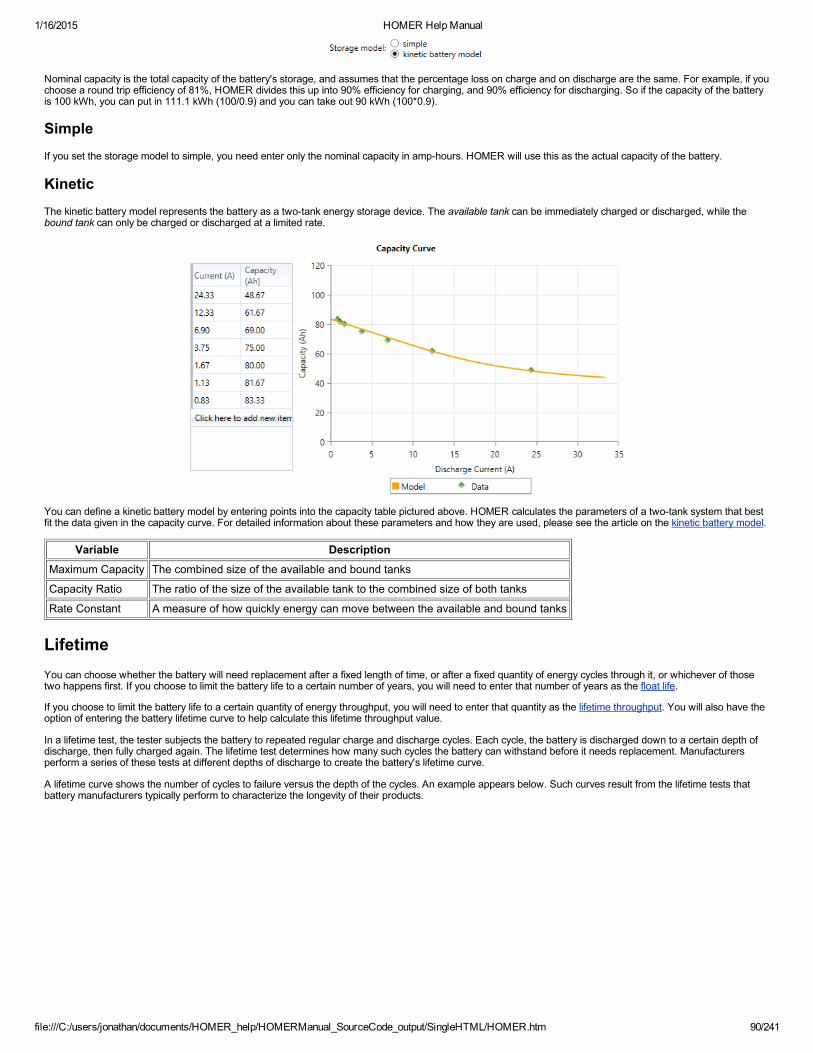
1/16/2015 HOMER Help Manual
file:///C:/users/jonathan/documents/HOMER_help/HOMERManual_SourceCode_output/SingleHTML/HOMER.htm 90/241
Nominal capacity is the total capacity of the battery's storage, and assumes that the percentage loss on charge and on discharge are the same. For example, if youchoose a round trip efficiency of 81%, HOMER divides this up into 90% efficiency for charging, and 90% efficiency for discharging. So if the capacity of the batteryis 100 kWh, you can put in 111.1 kWh (100/0.9) and you can take out 90 kWh (100*0.9).
SimpleIf you set the storage model to simple, you need enter only the nominal capacity in amphours. HOMER will use this as the actual capacity of the battery.
KineticThe kinetic battery model represents the battery as a twotank energy storage device. The available tank can be immediately charged or discharged, while thebound tank can only be charged or discharged at a limited rate.
You can define a kinetic battery model by entering points into the capacity table pictured above. HOMER calculates the parameters of a twotank system that bestfit the data given in the capacity curve. For detailed information about these parameters and how they are used, please see the article on the kinetic battery model.
Variable DescriptionMaximum Capacity The combined size of the available and bound tanks
Capacity Ratio The ratio of the size of the available tank to the combined size of both tanks
Rate Constant A measure of how quickly energy can move between the available and bound tanks
LifetimeYou can choose whether the battery will need replacement after a fixed length of time, or after a fixed quantity of energy cycles through it, or whichever of thosetwo happens first. If you choose to limit the battery life to a certain number of years, you will need to enter that number of years as the float life.
If you choose to limit the battery life to a certain quantity of energy throughput, you will need to enter that quantity as the lifetime throughput. You will also have theoption of entering the battery lifetime curve to help calculate this lifetime throughput value.
In a lifetime test, the tester subjects the battery to repeated regular charge and discharge cycles. Each cycle, the battery is discharged down to a certain depth ofdischarge, then fully charged again. The lifetime test determines how many such cycles the battery can withstand before it needs replacement. Manufacturersperform a series of these tests at different depths of discharge to create the battery's lifetime curve.
A lifetime curve shows the number of cycles to failure versus the depth of the cycles. An example appears below. Such curves result from the lifetime tests thatbattery manufacturers typically perform to characterize the longevity of their products.
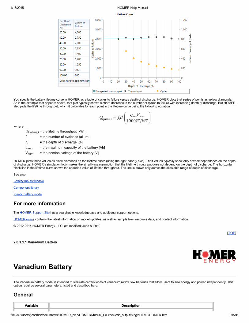
1/16/2015 HOMER Help Manual
file:///C:/users/jonathan/documents/HOMER_help/HOMERManual_SourceCode_output/SingleHTML/HOMER.htm 91/241
You specify the battery lifetime curve in HOMER as a table of cycles to failure versus depth of discharge. HOMER plots that series of points as yellow diamonds.As in the example that appears above, that plot typically shows a sharp decrease in the number of cycles to failure with increasing depth of discharge. But HOMERalso plots the lifetime throughput, which it calculates for each point in the lifetime curve using the following equation:
where:Qlifetime,i = the lifetime throughput [kWh]fi = the number of cycles to failuredi = the depth of discharge [%]qmax = the maximum capacity of the battery [Ah]Vnom = the nominal voltage of the battery [V]
HOMER plots these values as black diamonds on the lifetime curve (using the righthand yaxis). Their values typically show only a weak dependence on the depthof discharge. HOMER's simulation logic makes the simplifying assumption that the lifetime throughput does not depend on the depth of discharge. The horizontalblack line in the lifetime curve shows the specified value of lifetime throughput. The line is drawn only across the allowable range of depth of discharge.
See also
Battery Inputs window
Component library
Kinetic battery model
For more informationThe HOMER Support Site has a searchable knowledgebase and additional support options.
HOMER online contains the latest information on model updates, as well as sample files, resource data, and contact information.
© 20122014 HOMER Energy, LLCLast modified: June 8, 2010
[TOP]
2.8.1.1.1 Vanadium Battery
Vanadium Battery
The Vanadium battery model is intended to simulate certain kinds of vanadium redox flow batteries that allow users to size energy and power independently. Thisoption requires several parameters, listed and described here.
General
Variable Description

1/16/2015 HOMER Help Manual
file:///C:/users/jonathan/documents/HOMER_help/HOMERManual_SourceCode_output/SingleHTML/HOMER.htm 92/241
Round Trip Efficiency The round trip DCtostoragetoDC efficiency of the battery bank
Cell Stack Lifetime The lifetime of the cell stack. The cell stack replacement cost occurs at the end of the cell stack lifetime.
Electrolyte Lifetime The lifetime of the electrolyte. The electrolyte replacement cost occurs at the end of the electrolyte lifetime.
For more informationThe HOMER Support Site has a searchable knowledgebase and additional support options.
HOMER online contains the latest information on model updates, as well as sample files, resource data, and contact information.
© 20122014 HOMER Energy, LLCLast modified: October 21, 2009
[TOP]
2.8.1.1.2 Zinc Battery
Zinc Battery
The Zinc battery model is appropriate for some batteries that allow replacement of the cell stack and electrolyte seperately. This option requires severalparameters, listed in the table below.
General
Variable Description
Nominal Voltage The rated DC voltage. HOMER multiplies the nominal voltage by the nominal capacity in Ah to calculate the nominalcapacity in kWh.
Nominal Capacity The amount of energy that the battery stores at full charge
Round TripEfficiency The round trip DCtostoragetoDC efficiency of the battery bank
Lifetime The number of years the battery will last before it requires a complete replacement
Cell Stack Lifetime The number of years the cell stack will last before it needs replacement
Max Charge Current The maximum rate at which the system can put energy into the battery
Max DischargeCurrent The maximum rate at which the system can take energy out of the battery
For more informationThe HOMER Support Site has a searchable knowledgebase and additional support options.
HOMER online contains the latest information on model updates, as well as sample files, resource data, and contact information.
© 20122014 HOMER Energy, LLCLast modified: October 21, 2009
[TOP]
2.8.1.2 Generator
Generator
The Generator tab in the Generator window gives you access to the following variables:
Variable DescriptionAC The type of generator output current (alternating current or direct current)
Capacity

1/16/2015 HOMER Help Manual
file:///C:/users/jonathan/documents/HOMER_help/HOMERManual_SourceCode_output/SingleHTML/HOMER.htm 93/241
Nominal capacity (kW) of the generator. If the generator size is different in the search space, the fuel curve will be scaled.
Lifetime(OperatingHours)
The number of hours the generator can operate before needing replacement
Minimum LoadRatio The minimum allowable load on the generator expressed as a percentage of its capacity
Heat RecoveryRatio
The percentage of waste heat that can be used to serve the thermal load. If you are not modeling a thermal load or you do notintend to recover waste heat from the generator, set this to zero.
Cofire withBiogas
If selected, this allows access to inputs relating to the cofiring of a generator with a mixture of fossil fuel (usually diesel fuel,natural gas, or propane) and biogas
SubstitutionRatio The ratio with which the biogas replaces fossil fuel in the cofired generator, in %
Minimum FossilFraction The minimum allowable fossil fraction, in %, for a cofired generator
Derating Factor The relative capacity of the generator at the minimum fossil fraction, in %
Minimum RunTime Once the dispatch starts the generator, it will remain on for this duration or longer
Note: To the right of each numerical input is a sensitivity button ( )which allows you to do a sensitivity analysis on that variable. For more information, pleasesee Why would I want to do a sensitivity analysis?
For more informationThe HOMER Support Site has a searchable knowledgebase and additional support options.
HOMER online contains the latest information on model updates, as well as sample files, resource data, and contact information.
© 20122014 HOMER Energy, LLCLast modified: July 15, 2013
[TOP]
2.8.1.3 PV
Manufacturer PropertiesThe Manufacturer Properties box displays some basic information for the type of PV panel you have selected.
Variable DescriptionManufacturer The company that manufacturers the PV panel
Website The manufacturer's website
Type The type of PV technology
Abbreviation A short label used to identify the PV array
Notes Hints for modeling the PV system
[TOP]
2.8.1.4 Wind Turbine
Wind Turbine
This menu lets you view or specify the properties of the library wind turbines. You can create a new wind turbine from scratch or by copying an existing one.Change the properties as required and give the new wind turbine a unique name to distinguish it from others. HOMER will add this new wind turbine to yourcomponent library when you click OK. The new wind turbine will then be included in the list of available wind turbine types on the Wind Turbine Inputs window.
General
Variable DescriptionDescription A unique name used to identify this type of wind turbine
1/16/2015 HOMER Help Manual
file:///C:/users/jonathan/documents/HOMER_help/HOMERManual_SourceCode_output/SingleHTML/HOMER.htm 94/241
Abbreviation A short label which is used in column headings to identify this wind turbine
Manufacturer An optional field used to specify the manufacturer of the wind turbine
Website An optional field to hold the website of the manufacturer
Notes An optional field used to specify manufacturer contact information, prices, or anything noteworthy
Current Type The type of electricity produced by the wind turbine, either direct current (DC) or alternating current (AC)
Power curveThe power curve is the most important property of the wind turbine. It describes the amount of power the turbine produces versus the wind speed at hub height.
Enter as many points on the power curve as you have available. HOMER uses linear interpolation to calculate the output of the wind turbine at intervening points.
Written by: Tom Lambert ([email protected])Last modified: October 29, 2004
For more informationThe HOMER Support Site has a searchable knowledgebase and additional support options.
HOMER online contains the latest information on model updates, as well as sample files, resource data, and contact information.
© 20122014 HOMER Energy, LLCLast modified: October 29, 2004
[TOP]
2.8.1.5 Flywheel
Create New Flywheel
This window lets you view or specify the properties of library flywheels. You can create a new flywheel from scratch or by copying an existing one. Change theproperties as required and give the new wind turbine a unique name to distinguish it from others. HOMER will add this new flywheel to your component librarywhen you click OK. The new flywheel will then appear in the list of available flywheel types on the Flywheel Inputs window.
Properties
Variable DescriptionDescription A unique name used to identify this type of flywheel
Manufacturer An optional field used to specify the manufacturer of the flywheel
Website An optional field to hold the website of the manufacturer
Notes An optional field used to specify manufacturer contact information, prices, or anything noteworthy
Charge/DischargeCapacity
The maximum amount of power the flywheel can absorb or provide. (HOMER assumes that the flywheel's capacity to absorbpower is equal to its capacity to provide power.) This is the amount of operating capacity that the flywheel provides to thesystem.
Parasitic load The amount of electricity necessary to operate the flywheel. HOMER models this as a constant electrical load, and considersa system feasible only if it can meet this load at all times during the simulation.
See also
Flywheel Inputs window
Component library
Operating reserve
For more informationThe HOMER Support Site has a searchable knowledgebase and additional support options.
HOMER online contains the latest information on model updates, as well as sample files, resource data, and contact information.
© 20122014 HOMER Energy, LLCLast modified: January 21, 2010
[TOP]

1/16/2015 HOMER Help Manual
file:///C:/users/jonathan/documents/HOMER_help/HOMERManual_SourceCode_output/SingleHTML/HOMER.htm 95/241
2.8.2 Resources
Resources Library
The resources library contains saved resource definitions, and allows you to specify new resources. In this initial HOMER Pro release, only Fuels are implementedin the resource library. You can specify new fuels here, and access them from the Fuels dropdown menu in the Generator component. Solar, Wind, Temperature,Hydro and Biomass library resources are forthcoming.
See also
Create a New Fuel
For more informationThe HOMER Support Site has a searchable knowledgebase and additional support options.
HOMER online contains the latest information on model updates, as well as sample files, resource data, and contact information.
© 20122014 HOMER Energy, LLCLast modified: Sept 28, 2012
[TOP]
2.8.2.1 Create a New Fuel
Create a New Fuel
HOMER Pro users can create new fuels with specific properties. The properties are initially copied from the fuel that was selected when you clicked the Newbutton. Change the properties as required and give the new fuel a unique name to distinguish it from others. HOMER will add this new fuel to your componentlibrary when you click OK. The new fuel will then be included in the list of available fuel types on the Generator Inputs and Boiler Inputs windows.
Variable DescriptionDescription A unique name for the fuel
Lower Heating Value The energy released per kg of fuel consumed
Density Density in kg/m3 (the density of water is 1000 kg/m3)
Carbon Content The massbased carbon content of the fuel, in %
Sulfur Content The massbased sulfur content of the fuel, in %
Units The preferred units for amount and price of the fuel
For more informationThe HOMER Support Site has a searchable knowledgebase and additional support options.
HOMER online contains the latest information on model updates, as well as sample files, resource data, and contact information.
© 20122014 HOMER Energy, LLCLast modified: Sept 28, 2012
[TOP]
2.8.3 Grid
Grid Library
The grid library contains saved definitions of custom grid configurations. Here you can view existing grid definitions, modify advanced grid parameters, and savenew grid definitions that you can quickly add to any model.
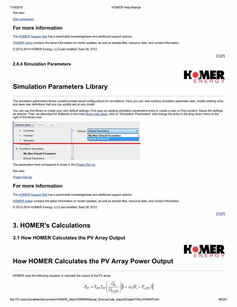
1/16/2015 HOMER Help Manual
file:///C:/users/jonathan/documents/HOMER_help/HOMERManual_SourceCode_output/SingleHTML/HOMER.htm 96/241
See also
Grid component
For more informationThe HOMER Support Site has a searchable knowledgebase and additional support options.
HOMER online contains the latest information on model updates, as well as sample files, resource data, and contact information.
© 20122014 HOMER Energy, LLCLast modified: Sept 28, 2012
[TOP]
2.8.4 Simulation Parameters
Simulation Parameters Library
The simulation parameters library contains preset saved configurations for simulations. Here you can view existing simulation parameter sets, modify existing ones,and save new definitions that you can quickly set on any model.
You can use this library to create your own default settings. First copy an existing simulation parameters entry or create a new on from scratch. Adjust the settingsas desired. Then, as described for Batteries in the main library help page, click on "Simulation Parameters" and change the entry in the drop down menu to theright of the library tree.
The parameters here correspond to those in the Project Set Up.
See also
Project Set Up
For more informationThe HOMER Support Site has a searchable knowledgebase and additional support options.
HOMER online contains the latest information on model updates, as well as sample files, resource data, and contact information.
© 20122014 HOMER Energy, LLCLast modified: Sept 28, 2012
[TOP]
3. HOMER's Calculations
3.1 How HOMER Calculates the PV Array Output
How HOMER Calculates the PV Array Power Output
HOMER uses the following equation to calculate the output of the PV array:

1/16/2015 HOMER Help Manual
file:///C:/users/jonathan/documents/HOMER_help/HOMERManual_SourceCode_output/SingleHTML/HOMER.htm 97/241
where:YPV is the rated capacity of the PV array, meaning its power output under standard test conditions [kW]fPV is the PV derating factor [%]
is the solar radiation incident on the PV array in the current time step [kW/m2]is the incident radiation at standard test conditions [1 kW/m2]
αP is the temperature coefficient of power [%/°C]Tc is the PV cell temperature in the current time step [°C]Tc,STC is the PV cell temperature under standard test conditions [25 °C]
If on the PV Inputs window you choose not to model the effect of temperature on the PV array, HOMER assumes that the temperature coefficient of power is zero,so that the above equation simplifies to:
See also
PV Inputs window
PV derating factor
PV temperature coefficient of power
Calculating the radiation incident on the PV array
Calculating the PV cell temperature
Standard test conditions
Can HOMER model a maximum power point tracker?
For more informationThe HOMER Support Site has a searchable knowledgebase and additional support options.
HOMER online contains the latest information on model updates, as well as sample files, resource data, and contact information.
© 20122014 HOMER Energy, LLCLast modified: November 15, 2007
[TOP]
3.2 Beacon Power Smart Energy 25 Flywheel
Beacon Power Smart Energy 25 Flywheel
The Smart Energy 25 is a 25 kWh, 100 kW carbon fiber flywheel. It is an AC device, but HOMER will connect it to the DC bus because it cannot model ACelectrical storage. To model this flywheel in HOMER, you should add a converter, but make it free, 100% efficient, and larger than the aggregate capacity of thelargest number of flywheels that you are considering. If your system also includes PV, we recommend modeling the PV as an AC device with the inverter costs andlosses included with the PV module.
In a hybrid power application, energy storage provides a buffer so that diesel generators can be turned off and remain off during short lulls in the wind or passingclouds. To maximize this benefit HOMER may use the full range of the energy storage device's state of charge before turning on another generator and rechargingthe device close to 100% state of charge.
For more informationThe HOMER Support Site has a searchable knowledgebase and additional support options.
HOMER online contains the latest information on model updates, as well as sample files, resource data, and contact information.
© 20122014 HOMER Energy, LLCLast modified: Nov. 9, 2010
[TOP]
3.3 How HOMER Calculates Emissions

1/16/2015 HOMER Help Manual
file:///C:/users/jonathan/documents/HOMER_help/HOMERManual_SourceCode_output/SingleHTML/HOMER.htm 98/241
How HOMER Calculates Emissions
HOMER calculates the emissions of the following six pollutants:
Pollutant DescriptionCarbon Dioxide (CO2) Nontoxic greenhouse gas.
Carbon Monoxide (CO)
Poisonous gas produced byincomplete burning of carbon infuels. Prevents delivery of oxygento the body's organs and tissues,causing headaches, dizziness, andimpairment of visual perception,manual dexterity, and learningability.
Unburned Hydrocarbons (UHC)
Products of incomplete combustionof hydrocarbon fuel, includingformaldehyde and alkenes. Leadto atmospheric reactions causingphotochemical smog.
Particulate Matter (PM)A mixture of smoke, soot, andliquid droplets that can causerespiratory problems and formatmospheric haze.
Sulfur Dioxide (SO2)
A corrosive gas released by theburning of fuels containing sulfur(like coal, oil and diesel fuel).Cause respiratory problems, acidrain, and atmospheric haze.
Nitrogen Oxides (NOx)
Various nitrogen compounds likenitrogen dioxide (NO2) and nitricoxide (NO) formed when any fuelis burned at high temperature.These compounds lead torespiratory problems, smog, andacid rain.
Emissions of these pollutants result from:
the production of electricity by the generator(s)the production of thermal energy by the boilerthe consumption of grid electricity
HOMER models the emissions of the generators and the boiler in a similar way, since both consume fuel of known properties. It models the grid slightly differently.This article will first cover how HOMER calculates the emissions of the generators and boiler, then how it calculates the emissions from the grid.
Generators, Boiler, and ReformerBefore simulating the power system, HOMER determines the emissions factor (kg of pollutant emitted per unit of fuel consumed) for each pollutant. After thesimulation, it calculates the annual emissions of that pollutant by multiplying the emissions factor by the total annual fuel consumption.
You directly specify the emissions factors for four of the six pollutants: carbon monoxide, unburned hydrocarbons, particulate matter, and nitrogen oxides. Usingthese values and the carbon and sulfur content of the fuel, HOMER does some calculations to find the emissions factors for the two remaining pollutants: carbondioxide and sulfur dioxide. In doing so, HOMER uses three principal assumptions:
1. Any carbon in the fuel that does not get emitted as carbon monoxide or unburned hydrocarbons gets emitted as carbon dioxide.2. The carbon fraction of the unburned hydrocarbon emissions is the same as that of the fuel.3. Any sulfur in the burned fuel that does not get emitted as particulate matter gets emitted as sulfur dioxide.
GridIn simulating a gridconnected system, HOMER calculates the net grid purchases, equal to the total grid purchases minus the total grid sales. To calculate theemissions of each pollutant associated with these net grid purchases, HOMER multiplies the net grid purchases (in kWh) by the emission factor (in g/kWh) for eachpollutant. If the system sells more power to the grid than it buys from the grid over the year, the net grid purchases will be negative and so will the gridrelatedemissions of each pollutant.
For more informationThe HOMER Support Site has a searchable knowledgebase and additional support options.
HOMER online contains the latest information on model updates, as well as sample files, resource data, and contact information.
© 20122014 HOMER Energy, LLCLast modified: Oct. 27, 2004

1/16/2015 HOMER Help Manual
file:///C:/users/jonathan/documents/HOMER_help/HOMERManual_SourceCode_output/SingleHTML/HOMER.htm 99/241
[TOP]
3.4 How HOMER Calculates the Hydro Power Output
How HOMER Calculates the Hydro Power Output
In each time step, HOMER calculates the electrical power output of the hydro turbine using the following equation:
where:Phyd = power output of the hydro turbine [kW]hhyd = hydro turbine efficiency [%]rwater = density of water [1000 kg/m3]g = acceleration due to gravity [9.81 m/s2]hnet = effective head [m]
= hydro turbine flow rate [m3/s]
See also
Nominal hydro power
For more informationThe HOMER Support Site has a searchable knowledgebase and additional support options.
HOMER online contains the latest information on model updates, as well as sample files, resource data, and contact information.
© 20122014 HOMER Energy, LLCLast modified: Dec 27, 2007
[TOP]
3.5 How HOMER Calculates Clearness Index
How HOMER Calculates Clearness Index
On the Solar Resource window, for each month of the year you can enter either the average radiation or the average clearness index. When you enter one,HOMER calculates the other. This article describes the relationship between the two variables, and how HOMER calculates one from the other.
The clearness index is a dimensionless number between 0 and 1 indicating the fraction of the solar radiation striking the top of the atmosphere that makes itthrough the atmosphere to strike the Earth's surface. The following equation defines the monthly average clearness index:
where:Have is the monthly average radiation on the horizontal surface of the earth [kWh/m2/day]
Ho,aveis the extraterrestrial horizontal radiation, meaning the radiation on a horizontal surface at the top of the earth's atmosphere[kWh/m2/day]
For a given latitude, we can calculate Ho,ave for any month of the year. So if we know either Have or KT , we can calculate the other using the above equation.HOMER does exactly that every time you enter a value into the monthly data table on the Solar Resource Inputs window. If you enter an average radiation value,HOMER will calculate the corresponding clearness index.
The rest of this article describes how HOMER calculates Ho,ave, the monthly average extraterrestrial radiation.
As described in more detail in the article on calculating the radiation incident on the PV array, HOMER uses the following equation to calculate the intensity of solar

1/16/2015 HOMER Help Manual
file:///C:/users/jonathan/documents/HOMER_help/HOMERManual_SourceCode_output/SingleHTML/HOMER.htm 100/241
radiation at the top of the Earth’s atmosphere:
where:Gsc is the solar constant [1.367 kW/m2]n is the the day of the year [a number between 1 and 365]
The equation above gives the extraterrestrial radiation on a surface normal to the sun's rays. To calculate the extraterrestrial radiation on the horizontal surface,HOMER uses the following equation:
where:qZ is the zenith angle [°]
HOMER calculates the zenith angle using the following equation:
where:f is the latitude [°]d is the solar declination [°]w is the hour angle [°]
HOMER calculates the solar declination according to the following equation:
where:n is the the day of the year [a number between 1 and 365]
We can find the total daily extraterrestrial radiation per square meter by integrating the equation for Go from sunrise to sunset. This integration gives the followingequation:
where:Ho is the average extraterrestrial horizonal radiation for the day [kWh/m2/day]ws is the sunset hour angle [°]
HOMER calculates the sunset hour angle using the following equation:
HOMER calculates Ho for each day of the month, and finds the average for the month as follows:
where:Ho,ave is the average extraterrestrial horizonal radiation for the month [kWh/m2/day]N is the number of days in the month
If you enter the monthly average global solar radiation, HOMER divides it by Ho,ave to find the monthly average clearness index.
See also
Clearness index
PV Inputs window
Calculating the radiation incident on the PV array
For more informationThe HOMER Support Site has a searchable knowledgebase and additional support options.
HOMER online contains the latest information on model updates, as well as sample files, resource data, and contact information.
© 20122014 HOMER Energy, LLCLast modified: November 15, 2007

1/16/2015 HOMER Help Manual
file:///C:/users/jonathan/documents/HOMER_help/HOMERManual_SourceCode_output/SingleHTML/HOMER.htm 101/241
[TOP]
3.6 How HOMER Calculates the Maximum Battery Charge Power
How HOMER Calculates the Maximum Battery ChargePower
In each time step, HOMER calculates the maximum amount of power that the battery bank can absorb. It uses this "maximum charge power" when makingdecisions such as whether the battery can absorb all available surplus renewable power, or how much surplus power a cycle charging generator should produce.The maximum charge power varies from one time step to the next according to its state of charge and its recent charge and discharge history.
HOMER imposes three separate limitations on the battery bank's maximum charge power. The first limitation comes from the kinetic battery model. As described inthe article on the kinetic battery model, the maximum amount of power that can be absorbed by the twotank system is given by the following equation:
whereQ1 is the available energy [kWh] in the battery at the beginning of the time step,Q is the total amount of energy energy [kWh] in the battery at the beginning of the time step,c is the battery capacity ratio [unitless],k is the battery rate constant [h1], andDt is the length of the time step [h].
The second limitation relates to the maximum charge rate of the battery, which is the A/Ah value visible on the battery details window. The battery charge powercorresponding to this maximum charge rate is given by the following equation:
whereac is the battery's maximum charge rate [A/Ah], andQmax is the total capacity of the battery bank [kWh].
The third limitation relates to the battery's maximum charge current, which also appears on the battery details window. The maximum battery bank charge powercorresponding to this maximum charge current is given by the following equation:
whereNbatt is the number of batteries in the battery bank,Imax is the battery's maximum charge current [A], andVnom is the battery's nominal voltage [V].
HOMER sets the maximum battery charge power equal to the least of these three values, assuming each applies after charging losses, hence:
where hbatt,c is the battery charge efficiency.
See also
Kinetic battery model
Calculating maximum battery discharge power
For more informationThe HOMER Support Site has a searchable knowledgebase and additional support options.
HOMER online contains the latest information on model updates, as well as sample files, resource data, and contact information.

1/16/2015 HOMER Help Manual
file:///C:/users/jonathan/documents/HOMER_help/HOMERManual_SourceCode_output/SingleHTML/HOMER.htm 102/241
© 20122014 HOMER Energy, LLCLast modified: July 22 2010
[TOP]
3.7 How HOMER Calculates the Maximum Battery Discharge Power
How HOMER Calculates the Maximum BatteryDischarge Power
In each time step, HOMER calculates the maximum amount of power that the battery bank can discharge. It uses this "maximum discharge power" when makingdecisions such as whether the battery can serve the load on its own. The maximum discharge power varies from one time step to the next according to its state ofcharge and its recent charge and discharge history, as determined by the kinetic battery model.
As described in the article on the kinetic battery model, the maximum amount of power that the battery bank can discharge over a specific length of time is given bythe following equation:
whereQ1 is the available energy [kWh] in the battery at the beginning of the time step,Q is the total amount of energy energy [kWh] in the battery at the beginning of the time step,Qmax is the total capacity [kWh] of the battery bank,c is the battery capacity ratio [unitless],k is the battery rate constant [h1], andDt is the length of the time step [h].
HOMER assumes that the discharging losses occur after the energy leaves the twotank system, hence the battery bank's maximum discharge power is given bythe following equation:
where hbatt,d is the battery discharge efficiency.
See also
Kinetic battery model
Calculating maximum battery charge power
For more informationThe HOMER Support Site has a searchable knowledgebase and additional support options.
HOMER online contains the latest information on model updates, as well as sample files, resource data, and contact information.
© 20122014 HOMER Energy, LLCLast modified: January 22, 2010
[TOP]
3.8 How HOMER Calculates the Radiation Incident on the PV Array
How HOMER Calculates the Radiation Incident on thePV Array
In the solar resource input window you specify, for each time step, the global horizontal radiation. That is the total amount of solar radiation striking the horizontalsurface on the earth. But the power output of the PV array depends on the amount of radiation striking the surface of the PV array, which in general is nothorizontal. So in each time step, HOMER must calculate the global solar radiation incident on the surface of the PV array. This article describes that process, which

1/16/2015 HOMER Help Manual
file:///C:/users/jonathan/documents/HOMER_help/HOMERManual_SourceCode_output/SingleHTML/HOMER.htm 103/241
is based on the methods in the first two chapters of Duffie and Beckman (1991)
We can describe the orientation of the PV array using two parameters, a slope and an azimuth. The slope is the angle formed between the surface of the paneland the horizontal, so a slope of zero indicates a horizontal orientation, whereas a 90° slope indicates a vertical orientation. The azimuth is the direction towardswhich the surface faces. HOMER uses the convention whereby zero azimuth corresponds to due south, and positive values refer to westfacing orientations. Soan azimuth of 45° corresponds to a southeastfacing orientation, and an azimuth of 90° corresponds to a westfacing orientation.
The other factors relevant to the geometry of the situation are the latitude, the time of year, and the time of day. The time of year affects the solar declination,which is the latitude at which the sun's rays are perpendicular to the earth's surface at solar noon. HOMER uses the following equation to calculate the solardeclination:
where:n is the day of the year [a number 1 through 365]
The time of day affects the location of the sun in the sky, which we can describe by an hour angle. HOMER uses the convention whereby the hour angle is zero atsolar noon (the time of day at which the sun is at its highest point in the sky), negative before solar noon, and positive after solar noon. HOMER uses the followingequation to calculate the hour angle:
where:ts is the solar time [hr]
The value of ts is 12hr at solar noon, and 13.5hr ninety minutes later. The above equation follows from the fact that the sun moves across the sky at 15 degrees perhour.
HOMER assumes that all timedependent data, such as solar radiation data and electric load data, are specified not in solar time, but in civil time, also called localstandard time. HOMER calculates solar time from civil time using the following equation:
where:tc is the civil time in hours corresponding to the midpoint of the time step [hr]λ is the longitude [°]Ζc is the time zone in hours east of GMT [hr]Ε is the equation of time [hr]
Note that west longitudes are negative, and time zones west of GMT are negative as well.
The equation of time accounts for the effects of obliquity (the tilt of the earth's axis of rotation relative to the plane of the ecliptic) and the eccentricity of the earth'sorbit. HOMER calculates the equation of time as follows:
where B is given by:
where n is the day of the year, starting with 1 for January 1st.
Now, for a surface with any orientation, we can define the angle of incidence, meaning the angle between the sun's beam radiation and the normal to the surface,using the following equation:
where:θ is the angle of incidence [°]β is the slope of the surface [°]γ is the azimuth of the surface [°]Φ is the latitude [°]δ is the solar declination [°]ω is the hour angle [°]

1/16/2015 HOMER Help Manual
file:///C:/users/jonathan/documents/HOMER_help/HOMERManual_SourceCode_output/SingleHTML/HOMER.htm 104/241
An incidence angle of particular importance, which we will need shortly, is the zenith angle, meaning the angle between a vertical line and the line to the sun. Thezenith angle is zero when the sun is directly overhead, and 90° when the sun is at the horizon. Because a horizontal surface has a slope of zero, we can find aequation for the zenith angle by setting Β = 0° in the above equation, which yields:
where:θz is the zenith angle [°]
Now we turn to the issue of the amount of solar radiation arriving at the top of the atmosphere over a particular point on the earth's surface. HOMER assumes theoutput of the sun is constant in time. But the amount of sunlight striking the top of the earth's atmosphere varies over the year because the distance between thesun and the earth varies over the year due to the eccentricity of earth's orbit. To calculate the extraterrestrial normal radiation, defined as the amount of solarradiation striking a surface normal (perpendicular) to the sun's rays at the top of the earth's atmosphere, HOMER uses the following equation:
where:Gon is the extraterrestrial normal radiation [kW/m2]Gsc is the solar constant [1.367 kW/m2]n is the day of the year [a number between 1 and 365]
To calculate the extraterrestrial horizontal radiation, defined as the amount of solar radiation striking a horizontal surface at the top of the atmosphere, HOMERuses the following equation:
where:Go is the extraterrestrial horizontal radiation [kW/m2]Gon is the extraterrestrial normal radiation [kW/m2]qz is the zenith angle [°]
Since HOMER simulates on a time step by time step basis, we integrate the above equation over one time step to find the average extraterrestrial horizontalradiation over the time step:
where:is the extraterrestrial horizontal radiation averaged over the time step [kW/m2]
Gon is the extraterrestrial normal radiation [kW/m2]w1 is the hour angle at the beginning of the time step [°]w2 is the hour angle at the end of the time step [°]
The above equation gives the average amount of solar radiation striking a horizontal surface at the top of the atmosphere in any time step. The solar resource datagive the average amount of solar radiation striking a horizontal surface at the bottom of the atmosphere (the surface of the earth) in every time step. The ratio of thesurface radiation to the extraterrestrial radiation is called the clearness index. The following equation defines the clearness index:
where:is the global horizontal radiation on the earth's surface averaged over the time step [kW/m2]is the extraterrestrial horizontal radiation averaged over the time step [kW/m2]
Now let us look more closely at the solar radiation on the earth's surface. Some of that radiation is beam radiation, defined as solar radiation that travels from thesun to the earth's surface without any scattering by the atmosphere. Beam radiation (sometimes called direct radiation) casts a shadow. The rest of the radiation isdiffuse radiation, defined as solar radiation whose direction has been changed by the earth's atmosphere. Diffuse radiation comes from all parts of the sky anddoes not cast a shadow. The sum of beam and diffuse radiation is called global solar radiation, a relation expressed by the following equation:
where:is the beam radiation [kW/m2]is the diffuse radiation [kW/m2]
The distinction between beam and diffuse radiation is important when calculating the amount of radiation incident on an inclined surface. The orientation of thesurface has a stronger effect on the beam radiation, which comes from only one part of the sky, than it does on the diffuse radiation, which comes from all parts ofthe sky.
However, in most cases we measure only the global horizontal radiation, not its beam and diffuse components. For that reason, HOMER expects you to enterglobal horizontal radiation in HOMER's Solar Resource Inputs window. That means that in every time step, HOMER must resolve the global horizontal radiationinto its beam and diffuse components to find the radiation incident on the PV array. For this purpose HOMER uses correlation of Erbs et al. (1982), which gives thediffuse fraction as a function of the clearness index as follows:

1/16/2015 HOMER Help Manual
file:///C:/users/jonathan/documents/HOMER_help/HOMERManual_SourceCode_output/SingleHTML/HOMER.htm 105/241
For each time step, HOMER uses the average global horizontal radiation to calculate the clearness index, then the diffuse radiation. It then calculates the beamradiation by subtracting the diffuse radiation from the global horizontal radiation.
We are now almost ready to calculate the global radiation striking the tilted surface of the PV array. For this purpose HOMER uses the HDKR model, whichassumes that there are three components to the diffuse solar radiation: an isotropic component which comes all parts of the sky equally, a circumsolar componentwhich emanates from the direction of the sun, and a horizon brightening component which emanates from the horizon. Before applying that model we must firstdefine three more factors.
The following equation defines Rb, the ratio of beam radiation on the tilted surface to beam radiation on the horizontal surface:
The anisotropy index, with symbol Ai, is a measure of the atmospheric transmittance of beam radiation. This factor is used to estimate the amount of circumsolardiffuse radiation, also called forward scattered radiation. The anisotropy index is given by the following equation:
The final factor we need to define is a factor used to account for 'horizon brightening', or the fact that more diffuse radiation comes from the horizon than from therest of the sky. This term is related to the cloudiness and is given by the following equation:
The HDKR model calculates the global radiation incident on the PV array according to the following equation:
where:b is the slope of the surface [°]rg is the ground reflectance, which is also called the albedo [%]
HOMER uses this quantity to calculate the cell temperature and the power output of the PV array.
See also
Solar Resource Inputs window
Clearness index
How HOMER calculates the PV cell temperature
How HOMER calculates the PV array power output
For more informationThe HOMER Support Site has a searchable knowledgebase and additional support options.
HOMER online contains the latest information on model updates, as well as sample files, resource data, and contact information.
© 20122014 HOMER Energy, LLCLast modified: November 7, 2007
[TOP]
3.9 How HOMER Calculates Wind Turbine Power Output
How HOMER Calculates Wind Turbine Power Output
HOMER calculates the power output of the wind turbine in each time step. This entails a threestep process to first calculate the wind speed at the hub height ofthe wind turbine, then to calculate how much power the wind turbine would produce at that wind speed at standard air density, then to adjust that power outputvalue for the actual air density.

1/16/2015 HOMER Help Manual
file:///C:/users/jonathan/documents/HOMER_help/HOMERManual_SourceCode_output/SingleHTML/HOMER.htm 106/241
Calculating Hub Height Wind SpeedIn each time step, HOMER calculates the wind speed at the hub height of the wind turbine using the inputs you specify in the Wind Resource Inputs window andthe Wind Shear Inputs window.
If you choose to apply the logarithmic law, HOMER calculates the hub height wind speed using the following equation:
where:Uhub = the wind speed at the hub height of the wind turbine [m/s]Uanem = the wind speed at anemometer height [m/s]zhub = the hub height of the wind turbine [m]zanem = the anemometer height [m]z0 = the surface roughness length [m]ln(..) = the natural logarithm
If you choose to apply the power law, HOMER calculates the hub height wind speed using the following equation:
where:Uhub = the wind speed at the hub height of the wind turbine [m/s]
Uanem = the wind speed at anemometer height [m/s]zhub = the hub height of the wind turbine [m]zanem = the anemometer height [m]a = the power law exponent
Calculating Turbine Power Output At Standard Air DensityOnce HOMER has determined the hub height wind speed, it refers to the wind turbine's power curve to calculate the power output one would expect from thatwind turbine at that wind speed under standard conditions of temperature and pressure. In the diagram below, the red dotted line indicates the hub height windspeed, and the blue dotted line indicates the wind turbine power output that the power curve predicts for that wind speed.
Applying Density CorrectionPower curves typically specify wind turbine performance under conditions of standard temperature and pressure (STP). To adjust to actual conditions, HOMERmultiplies the power value predicted by the power curve by the air density ratio, according to following equation:
where:PWTG = the wind turbine power output [kW]PWTG,STP = the wind turbine power output at standard temperature and pressure [kW]r = the actual air density [kg/m3]

1/16/2015 HOMER Help Manual
file:///C:/users/jonathan/documents/HOMER_help/HOMERManual_SourceCode_output/SingleHTML/HOMER.htm 107/241
r0 = the air density at standard temperature and pressure (1.225 kg/m3)
See also
Wind Resource Inputs window
Wind Shear Inputs window
Altitude
For more informationThe HOMER Support Site has a searchable knowledgebase and additional support options.
HOMER online contains the latest information on model updates, as well as sample files, resource data, and contact information.
© 20122014 HOMER Energy, LLCLast modified: October 8, 2009
[TOP]
3.10 Operation of a Cofired Generator
Operation of a Cofired Generator
A cofired generator operates on a mixture of fossil fuel and biogas. In each time step, HOMER calculates the required output of the generator and thecorresponding mass flow rates of fossil fuel and biogas. This calculation is based on several key assumptions:
Assumptions:
1. The biogas substitution ratio (zgas) is a constant, independent of engine output power or fuel mixture.2. The system will at all times attempt to maximize the use of biogas and minimize the use of fossil fuel.3. The fossil fraction cannot go below a certain minimum.4. Even if the derating factor associated with operating in dualfuel mode is less than 100%, the generator can produce up to 100% of its rated power provided
the fossil fraction is high enough.
The fuel curve of a cofired generator defines the fuel consumption of the generator in pure fossil mode. So the fossil fuel consumption in pure fossil mode is givenby the following equation: (please see table of nomenclature below for a definition of all symbols)
(1)
And from assumption 1,
(2)
Where zgas is the biogas substitution ratio. Now from the definition of the fossil fraction,
(3)
Using equations 2 and 3,
(4)
But for a given value of Pbio, the value of xfossil is unknown so the above equation is not enough on its own to solve for the biogas flow rate. From assumption 2,we want to maximize , which means we want to minimize xfossil. But from assumption 3,

1/16/2015 HOMER Help Manual
file:///C:/users/jonathan/documents/HOMER_help/HOMERManual_SourceCode_output/SingleHTML/HOMER.htm 108/241
where is the minimum fossil fraction required for ignition. So the target value for corresponds to . Using equation 4,
(5)
But there are two independent upper limits on the actual value of . At the minimum fossil fraction, the output of the generator is limited to , defined asfollows:
where t, the derating factor, is less than or equal to 1. This limitation can be implemented by imposing an upper limit on corresponding to and . Usingequations 1 and 4, this maximum value can be defined as:
(6)
This upper limit can be thought of as a physical limitation the maximum rate at which biogas can be ingested in the engine. The available biomass resource, agas,
constitutes the other upper limit on . So the actual value of is the minimum of , , and agas:
(7)
Knowing the value of , we can determine xfossil. Solving equation 4 for xfossil,
(8)
And from equation 3,
(9)
So at any time step, given particular values of Pbio and agas, the biogas flow rate and the fossil fuel flow rate can be calculated from equations 7 and 9,respectively.
Table of NomenclatureSymbol Units Descriptionrfossil kg/L density of fossil fuelt % generator derating factoragas kg/hr available biogas flow rate
kg/hr fossil fuel flow rate (in pure fossil mode)kg/hr fossil fuel flow rate (in dualfuel mode)kg/hr biogas flow rate (in dualfuel mode)kg/hr maximum value of biogas flow ratekg/hr target value of biogas flow rate
xfossil % fossil fraction% minimum fossil fraction
zgas none biogas substitution ratio
F0 L/hr/kW generator fuel curve interceptcoefficient
F1 L/hr/kW generator fuel curve slopePgen kW power output of the generator
kW maximum output of generator atminimum fossil fraction
Ygen kW rated capacity of the generator
For more informationThe HOMER Support Site has a searchable knowledgebase and additional support options.
HOMER online contains the latest information on model updates, as well as sample files, resource data, and contact information.
© 20122014 HOMER Energy, LLCLast modified: June 18, 2004
[TOP]

1/16/2015 HOMER Help Manual
file:///C:/users/jonathan/documents/HOMER_help/HOMERManual_SourceCode_output/SingleHTML/HOMER.htm 109/241
3.11 How HOMER Creates the Generator Efficiency Curve
How HOMER Creates the Generator Efficiency Curve
On the Generator Inputs window, when you enter the fuel curve inputs HOMER draws the corresponding efficiency curve. This article explains how HOMERcreates that graph from the fuel curve inputs.
Fuel unitsYou may have noticed that the units of the fuel curve inputs sometimes change when you select a different fuel from the dropdown box. That's because inHOMER, fuels can be denominated in units of kg, L, or m3. When you create a new fuel, you choose which units you want to use for that fuel. For example, youmay choose to denominate liquid fuels (e.g. diesel, gasoline, ethanol) in L, and gaseous fuels (e.g. natural gas, hydrogen) in m3. Once you have created a fuel, allthe inputs that relate to that fuel will use the specified units. For example, if diesel fuel is denominated in L, then the price of diesel fuel will be in $/L and the fuelcurve inputs for a diesel generator will be in L/hr/kW. Similarly, if natural gas is denominated in m3 then its price will be in $/m3 and the fuel curve inputs for anatural gas engine will be in m3/hr/kW. This article uses the term "units" to mean the units specified for the particular fuel, whether kg, L, or m3. For example,"units/hr" means L/hr for a fuel denominated in L, and kg/hr for a fuel denominated in kg.
Fuel curveThe fuel curve describes the amount of fuel the generator consumes to produce electricity. HOMER assumes that the fuel curve is a straight line. The followingequation gives the generator's fuel consumption in units/hr as a function of its electrical output:
where F0 is the fuel curve intercept coefficient in units/hr/kW, F1 is the fuel curve slope in units/hr/kW, Ygen is the rated capacity of the generator in kW, and Pgen isthe electrical output of the generator in kW.
Efficiency curveIn HOMER, we define the generator's electrical efficiency as the electrical energy coming out divided by the chemical energy of the fuel going in. The followingequation gives this relationship:
where Pgen is the electrical output in kW, mfuel is the mass flow rate of the fuel in kg/hr and LHVfuel is the lower heating value (a measure of energy content) of thefuel in MJ/kg. The factor of 3.6 arises because 1 kWh = 3.6 MJ.
The mass flow rate of the fuel is related to F, the generator's fuel consumption, but the exact relationship depends on the units of the fuel. If the fuel units are kg,then mfuel and F are equal, so the equation for mfuel is as follows:
If the fuel units are L, the relationship between mfuel and F involves the density. The equation for mfuel is as follows:
where rfuel is the fuel density in kg/m3. If the fuel units are m3 the factor of 1000 is unnecessary, and the equation for mfuel is as follows:
Let us further develop the efficiency equation for the case where the fuel units are L. In this case, the efficiency equation becomes:
If we divide numerator and denominator by Ygen, the capacity of the generator, and define a new symbol pgen for the relative output of the generator (pgen =Pgen/Ygen) then the efficiency equation becomes:

1/16/2015 HOMER Help Manual
file:///C:/users/jonathan/documents/HOMER_help/HOMERManual_SourceCode_output/SingleHTML/HOMER.htm 110/241
That equation gives the efficiency of the generator as a function of its relative output. It is this relation that HOMER plots in the efficiency curve on the GeneratorInputs window when the fuel units are L.
If the fuel units are m3, the efficiency equation becomes:
Finally, if the fuel units are kg, the efficiency equation becomes:
Example
For an example, let's analyze a 75 kW generator that burns diesel. Assume diesel has a density of 820 kg/m3 and a lower heating value of 43.2 MJ/kg. If thegenerator consumes 22.5 L/hr at full load and 10.5 L/hr at 25 kW, what does its efficiency curve look like?
First we need to calculate the fuel curve slope and intercept coefficient. We assume (as we must in HOMER) that the fuel curve is a straight line passing throughthe two given points, as shown in the graph below.
Note that if we were given more than two points on this curve, we could calculate the line of best fit, using a linear regression technique for example. But since weare given only two points, we can directly calculate the slope and intercept of the line that passes through those points.
We can find the slope and intercept of that line as follows:
Note that HOMER's first fuel curve input is not the intercept itself, but rather the intercept coefficient, defined as the intercept divided by the rated capacity of thegenerator. (This is so that HOMER can apply the fuel curve inputs to each generator size that you specify in the Sizes to consider table.) So the two fuel curveinputs are:
Since this is a liquid fuel denominated in L, the appropriate efficiency equation is:
So we can substitute our values of density, lower heating value, and fuel curve as follows:
Therefore the efficiency is 33.9% at full load (pgen= 1), 28.2% at 50% load, 18.8% at 20% load, and 7.0% at 5% load. The efficiency curve is shown below:

1/16/2015 HOMER Help Manual
file:///C:/users/jonathan/documents/HOMER_help/HOMERManual_SourceCode_output/SingleHTML/HOMER.htm 111/241
For more informationThe HOMER Support Site has a searchable knowledgebase and additional support options.
HOMER online contains the latest information on model updates, as well as sample files, resource data, and contact information.
© 20122014 HOMER Energy, LLCLast modified: May 6, 2004
[TOP]
3.12 Kinetic Battery Model
Kinetic Battery Model
HOMER uses the Kinetic Battery Model (Manwell and McGowan, 1993) to determine the amount of energy that can be absorbed by or withdrawn from the batterybank each time step. The kinetic battery model, so named because it is based on the concepts of electrochemical kinetics, models a battery as a two tank system.The first tank contains "available energy", or energy that is readily available for conversion to DC electricity. The second tank contains "bound energy", or energythat is chemically bound and therefore not immediately available for withdrawal. The following diagram illustrates the concept:
Three parameters are used to describe this two tank system. The maximum (or theoretical) battery capacity (Qmax) is the total amount of energy the two tanks cancontain. The capacity ratio (c) is the ratio of the size of the available energy tank to the combined size of both tanks. The rate constant (k) relates to theconductance between the two tanks, and is therefore a measure of how quickly the battery can convert bound energy to available energy or viceversa. HOMERdetermines these three parameters from the battery's capacity curve, which you specify in the Create New Battery window.
The total amount of energy stored in the battery at any time is the sum of the available and bound energy, hence:
where Q1 is the available energy and Q2 is the bound energy.
Using differential equations, one can show that the maximum amount of power that the battery can discharge over a specific length of time Dt is given by thefollowing equation:
Similarly, the maximum amount of power that the battery can absorb over a specific length of time is given by the following equation:
The preceding two equations give the allowable range for the power into or out of the battery bank in any one time step. (HOMER imposes two additionallimitations on the charge power. For more information please see the article on calculating the maximum charge power. Once HOMER calculates the actual chargeor discharge power, it calculates the resulting amount of available and bound energy at the end of the time step using the following two equations:
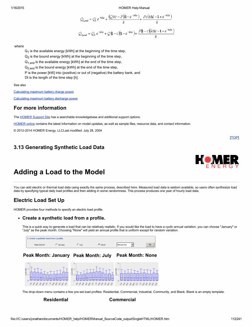
1/16/2015 HOMER Help Manual
file:///C:/users/jonathan/documents/HOMER_help/HOMERManual_SourceCode_output/SingleHTML/HOMER.htm 112/241
whereQ1 is the available energy [kWh] at the beginning of the time step,Q2 is the bound energy [kWh] at the beginning of the time step,Q1,end is the available energy [kWh] at the end of the time step,Q2,end is the bound energy [kWh] at the end of the time step,P is the power [kW] into (positive) or out of (negative) the battery bank, andDt is the length of the time step [h].
See also
Calculating maximum battery charge power
Calculating maximum battery discharge power
For more informationThe HOMER Support Site has a searchable knowledgebase and additional support options.
HOMER online contains the latest information on model updates, as well as sample files, resource data, and contact information.
© 20122014 HOMER Energy, LLCLast modified: July 28, 2004
[TOP]
3.13 Generating Synthetic Load Data
Adding a Load to the Model
You can add electric or thermal load data using exactly the same process, described here. Measured load data is seldom available, so users often synthesize loaddata by specifying typical daily load profiles and then adding in some randomness. This process produces one year of hourly load data.
Electric Load Set UpHOMER provides four methods to specify an electric load profile.
Create a synthetic load from a profile.This is a quick way to generate a load that can be relatively realistic. If you would like the load to have a cyclic annual variation, you can choose "January" or"July" as the peak month. Choosing "None" will yield an annual profile that is uniform except for random variation.
Peak Month: January Peak Month: July Peak Month: None
The dropdown menu contains a few preset load profiles: Residential, Commercial, Industrial, Community, and Blank. Blank is an empty template.
Residential Commercial

1/16/2015 HOMER Help Manual
file:///C:/users/jonathan/documents/HOMER_help/HOMERManual_SourceCode_output/SingleHTML/HOMER.htm 113/241
Industrial Community
These load templates all have different default overall magnitudes: 11.35, 2620, 24000, and 170 kWh/day respectively. You can easily scale the average loadof any of them to fit your application by changing the value for "Scaled Annual Average (kWh/day)".
Import a load from a time series file.
To import a file, you must prepare a text file that contains the electric load in each time step for a complete year.
Tip: You can import data with any time step down to one minute. HOMER detects the time step when you import the data file. For example, if the data filecontains 8760 lines, HOMER will assume that it contains hourly data. If the data file contains 52,560 lines, HOMER will assume that it contains 10minutedata.
The data file must contain a single value on each line, where each line corresponds to one time step. Each value in the file represents the average load (inkW) for that time step. The first time step starts at midnight on January 1st. A sample input file appears below.
When you import data from a text file, HOMER makes a copy of the data set and integrates it with the HOMER (.hmr) file. Once the data is part of theHOMER file, HOMER no longer refers to the original text file. If you modify data in the original file, you must import the modified file in order for themodification to be included in the HOMER file. After you import a data file, HOMER calculates the average 24hour load profile for the whole year displays itin the table and graph. HOMER also displays the name of the imported data file in the title of the load profile graph.
If you click Enter daily load profile(s) after importing data from a file, HOMER discards the data from the imported file and synthesizes new data based on thetwelve monthly average load profiles it calculated from the imported data. You can edit synthesized data by selecting the month and changing values in theload profile table. To edit values from an imported file, you must edit the file directly and then import the modified file, as described above.
Build a synthetic load using measured data.
You can import load data for specific devices as a CSV file with 24 hours of data, either in hourly or minuteresolution. Refer to the chart below forappropriate formatting. The first row and first two columns are ignored, reserved for user row titles if desired. The second row (column 3 and onward,

1/16/2015 HOMER Help Manual
file:///C:/users/jonathan/documents/HOMER_help/HOMERManual_SourceCode_output/SingleHTML/HOMER.htm 114/241
highlighted below in yellow) should contain descriptive names for each device. Row 3 through row 1442 (or row 3 through 26 for hourly data, below inorange) contains the load profile for each device in watts.
Note that HOMER will accept a mix of 1440row and 24row data columns in a single document. HOMER will infer the time step based on the number ofrows of data for each column individually.
Select the "Open Equipment Database" button in the upper right corner of the Load Designer menu, choose "Open...", and select your csv file. The loaddesigner will import each column in the file as a separate device. You can drag and drop rows from the Equipment Database popup into the Load Designer.Once you are done, close the Equipment Database popup. You can now edit the quantities of each item, if desired. You can also set the "Jitter", whichoffsets the load profiles randomly so that load peaks in the duplicate devices (if set to quantity greater than one) will not always line up exactly.
Choose a load from the library.Choose this option to retrieve load profiles from the HOMER Library.
For more informationThe HOMER Support Site has a searchable knowledgebase and additional support options.
HOMER online contains the latest information on model updates, as well as sample files, resource data, and contact information.
© 20122014 HOMER Energy, LLCLast modified: July 23, 2014
[TOP]
3.14 Generating Synthetic Solar Data
Generating Synthetic Solar Data
NEEDS UPDATING
SCREENSHOTS
When you do not have access to measured solar radiation data, you can use HOMER's capability to generate synthetic hourly solar data from monthly averagedata. HOMER synthesizes hourly solar radiation data using an algorithm based on the work of V.A. Graham. We have found this algorithm to produce realistichourly data, and it is easy to use because it requires only the latitude and the twelve monthly average values.
The realistic nature of synthetic data created by this algorithm is demonstrated in the two DMaps below. The first shows the measured TMY2 solar data for Seattle,WA. The second shows the synthetic data created by specifying Seattle's latitude and monthly average radiation values. The synthetic data display realistic daytoday and hourtohour patterns. If one hour is cloudy, there is a relatively high likelihood that the next hour will also be cloudy. Similarly, one cloudy day is likely to befollowed by another cloudy day.

1/16/2015 HOMER Help Manual
file:///C:/users/jonathan/documents/HOMER_help/HOMERManual_SourceCode_output/SingleHTML/HOMER.htm 115/241
The algorithm creates synthetic solar data with certain statistical properties that reflect global averages. So data generated for a particular location will not perfectlyreplicate the characteristics of the real solar resource. But our tests show that synthetic solar data produce virtually the same simulation results as real data.Differences in key performance output variables like annual PV array production, fuel consumption, generator run time, and battery throughput are typically lessthan 5%. Differences in key economic output variables like total net present cost and levelized cost of energy are typically less than 2%.
To generate synthetic solar data, go to the Solar Resource window. For each month enter either the average clearness index or the average daily radiation. If youenter the clearness index, HOMER will calculate the average daily radiation, and vice versa, using the latitude. For details, see the article on how HOMERcalculates clearness index.
For assistance in finding monthly solar data, see Finding data to run HOMER
See also
How HOMER calculates clearness index
For more informationThe HOMER Support Site has a searchable knowledgebase and additional support options.
HOMER online contains the latest information on model updates, as well as sample files, resource data, and contact information.
© 20122014 HOMER Energy, LLCLast modified: October 27, 2004
[TOP]
3.15 Generating Synthetic Wind Data
Generating Synthetic Wind Data
When you have no access to measured wind speed data, you can create time series wind speed data using HOMER's synthetic wind speed data synthesisalgorithm. This algorithm requires you to enter a few parameters, from which it generates artificial but statistically reasonable time series data. The algorithmproduces data that mimic the characteristics of real wind speed data, including strong and sustained gusts, long lulls between windy periods, and seasonal anddiurnal patterns.
Tip: When you import measured wind speed data, it can have any time step down to one minute. Similarly, when you generate synthetic wind data, it can have anytime step down to one minute.
ParametersTo generate synthetic wind speed data, go to the Wind Resources Inputs window and choose Enter monthly averages. You must enter the twelve monthly averagewind speeds, as well as the following four parameters:
Parameter DescriptionWeibull k Reflects the breadth of the distribution of wind speeds over the year.1hour autocorrelation factor Reflects how strongly the wind speed in one time step tends to depend on the wind speed in the previous time step.Diurnal pattern strength Reflects how strongly the wind speed depends on the time of day.Hour of peak wind speed The hour of day that tends to be windiest on average.
One can estimate the value of each of these parameters without detailed knowledge of the wind data in a particular location. The articles on each of the parametersgive guidance for doing so.
AlgorithmHOMER follows a fivestep process to synthesize one year of time series wind speed data:
Step 1

1/16/2015 HOMER Help Manual
file:///C:/users/jonathan/documents/HOMER_help/HOMERManual_SourceCode_output/SingleHTML/HOMER.htm 116/241
In the first step of the algorithm, HOMER generates a sequence of autocorrelated numbers, one for each time step of the year, using the firstorder autoregressivemodel:
where:zt = the value in time step izt1
= the value in time step i1
a = the autoregressive parameter
f(t) = a 'white noise' function that returns a random number drawn from a normal distribution with mean of zero and a standard deviation of1
HOMER sets the autoregressive parameter equal to the onetimestep autocorrelation coefficient:
But on the Wind Resource Inputs window you enter the onehour autocorrelation coefficient, which is different from the onetimestep autocorrelation coefficient ifthe time step is not 60 minutes.
To calculate the onetimestep autocorrelation coefficient from the onehour autocorrelation factor, HOMER assumes logarithmic decay in the autocorrelationfunction, in which case the following equation gives the autocorrelation parameter for a lag of k time steps:
Solving that for r1 gives:
The onehour autocorrelation factor is rk where k is the number of time steps that fit in one hour, meaning:
Where t is the time step in minutes.
This first step of the algorithm produces a series of numbers that conform to a normal distribution with a mean of zero and a standard deviation of 1.
Step 2In the second step of the algorithm, HOMER creates a full year of data by piecing together the desired average diurnal wind speed profile, repeated every day.Because the average wind speed varies by month, the average diurnal wind speed profile scales to a different value each month, but within each month the diurnalpattern simply repeats over and over.
Step 3In the third step, HOMER performs a probability transformation on the sequence of numbers generated in Step 2 so that it conforms to the same normal distributionas the sequence generated in Step 1.
Step 4In the fourth step, HOMER adds the sequence generated in Step 3 to the sequence generated in Step 1. The resulting sequence conforms to a normal distribution,but exhibits the desired degree of autocorrelation.
Step 5In the fifth and final step, HOMER performs a probability transformation on the sequence generated in Step 4 to make it conform to the desired Weibull distribution.
The two DMaps below demonstrate the results of the synthetic wind data generation algorithm. The first shows the measured wind speed data for San Francisco,California from the TMY2 data set. The second shows the synthetic wind speed data that HOMER generated from the monthly average wind speeds and the fourwind data parameters measured from the real data:
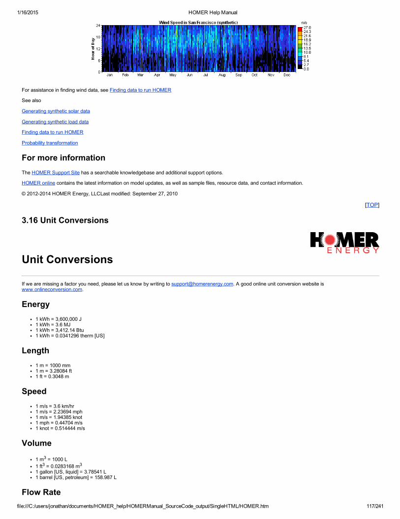
1/16/2015 HOMER Help Manual
file:///C:/users/jonathan/documents/HOMER_help/HOMERManual_SourceCode_output/SingleHTML/HOMER.htm 117/241
For assistance in finding wind data, see Finding data to run HOMER
See also
Generating synthetic solar data
Generating synthetic load data
Finding data to run HOMER
Probability transformation
For more informationThe HOMER Support Site has a searchable knowledgebase and additional support options.
HOMER online contains the latest information on model updates, as well as sample files, resource data, and contact information.
© 20122014 HOMER Energy, LLCLast modified: September 27, 2010
[TOP]
3.16 Unit Conversions
Unit Conversions
If we are missing a factor you need, please let us know by writing to [email protected]. A good online unit conversion website iswww.onlineconversion.com.
Energy1 kWh = 3,600,000 J1 kWh = 3.6 MJ1 kWh = 3,412.14 Btu1 kWh = 0.0341296 therm [US]
Length1 m = 1000 mm1 m = 3.28084 ft1 ft = 0.3048 m
Speed1 m/s = 3.6 km/hr1 m/s = 2.23694 mph1 m/s = 1.94385 knot1 mph = 0.44704 m/s1 knot = 0.514444 m/s
Volume
1 m3 = 1000 L1 ft3 = 0.0283168 m3
1 gallon [US, liquid] = 3.78541 L1 barrel [US, petroleum] = 158.987 L
Flow Rate

1/16/2015 HOMER Help Manual
file:///C:/users/jonathan/documents/HOMER_help/HOMERManual_SourceCode_output/SingleHTML/HOMER.htm 118/241
1 m3/s = 1000 L/s1 ft3/min [or cfm] = 0.4719475 L/s1 ft3/s [or cfs] = 28.316847 L/s1 gallon/min [US] = 0.0630902 L/s
Weight/Mass1 kg = 1000 g1 t [tonne] = 1,000 kg1 kg = 2.20462 lb1 lb = 0.453592 kg1 ton [short] = 907.185 kg1 ton [long] = 1,016.05 kg
For more informationThe HOMER Support Site has a searchable knowledgebase and additional support options.
HOMER online contains the latest information on model updates, as well as sample files, resource data, and contact information.
© 20122014 HOMER Energy, LLCLast modified: August 10, 2004
[TOP]
4. Finding data to run HOMER
Finding Data to Run HOMER
One of the biggest challenges in using a model like HOMER is finding the numbers to put into it. This page is meant to help you find the information you need. Ifyou know of any other helpful sources, please let us know so we can add them. Note that NREL cannot guarantee the accuracy of any data from externalsources, and does not endorse any manufacturer or retailer.
Electric Load DataThe only source of hourly load data that we're aware of is the DG Marketplace, which you can visit at www.dgmarketplace.com. This website sells typicalresidential, commercial, and industrial load data for locations across the US.
GeographyTo find your latitude and longitude, check maps.google.com. For help with Google Maps, see this Google Support article about latitude and longitude: Latitude andlongitude coordinates).
To find your time zone, check www.worldtimezone.com.
Solar Radiation DataHOMER will accept solar radiation data as monthly averages or as a time series. Time series solar radiation data is most commonly available with an hourly timestep, but HOMER can accept any time step down to one minute. One of the best sources of solar radiation data is the TMY2 and TMY3 data sets provided for freeby the US National Renewable Energy Laboratory. You can import TMY2 and TMY3 files directly into HOMER's Solar Resource Inputs window.
NREL provides TMY2 data at: http://rredc.nrel.gov/solar/old_data/nsrdb/19611990/tmy2/).And TMY3 data at: http://rredc.nrel.gov/solar/old_data/nsrdb/19912005/tmy3/).NASA's Surface Solar Energy Data Set provides monthly average solar radiation data for everywhere on earth at http://eosweb.larc.nasa.gov/sse/.This help file contains a table of monthly solar data for selected worldwide locations.The US Renewable Resource Data Center provides US data and maps at www.nrel.gov/rredc/solar_resource.html.The World Radiation Data Center provides worldwide solar data at http://wrdcmgo.nrel.gov. Note that data from this website need a lot of processing to beuseful in HOMER.GeoModel Solar has many solar data sets available at various resolutions: http://solargis.info.
Wind Speed DataIt can be difficult to obtain measured wind speed data. Proper measurement of wind speed is expensive and time consuming, and average wind speeds can varymarkedly over short distances because of terrain effects. For these reasons, it is often necessary to synthesize wind data from estimated monthly average windspeeds.
Many countries have published wind atlases:
Wind maps for many US states are available at apps2.eere.energy.gov/wind/windexchange/windmaps/.

1/16/2015 HOMER Help Manual
file:///C:/users/jonathan/documents/HOMER_help/HOMERManual_SourceCode_output/SingleHTML/HOMER.htm 119/241
The Canadian Wind Atlas is available at www.windatlas.ca.The Brazilian Wind Atlas is available at www.cresesb.cepel.br/publicacoes/index.php?task=livro&cid=1.
A number of other websites provide wind speed data:
The US Renewable Resource Data Center provides information on wind data at http://www.nrel.gov/rredc/wind_resource.html.The website www.weatherbase.com provides monthly average wind speed data for many cities around the world.The Windustry website maintains a list of US wind data resources at www.windustry.com/resources/windmaps.htm.The US National Climatic Data Center provides monthly average wind speed data for many US cities at http://www1.ncdc.noaa.gov/pub/data/ccddata/wndspd12.txt. To convert from mph to m/s, divide by 2.23694.The Technical University of Denmark maintains a database of wind characteristics at www.winddata.com.
Renewable Power System ComponentsSeveral retailers sell components for renewable power systems . The website www.ecobusinesslinks.com maintains a list of renewable power retailers around theworld. A few have very helpful websites providing cost and performance data for PV panels, wind turbines, hydro turbines, batteries, converters, and other systemcomponents. Check out:
The Alternative Energy Store at www.altenergystore.comSolarEnergy.com at www.solarenergy.comThe Solar Biz at www.thesolarbiz.comThe Energy Development Cooperative at www.unlimitedpower.co.uk
Other sources of cost and performance data for renewable power system components include:
The Renewable Energy Technology Characterizations, a detailed report on the performance and costs of solar, wind, and biomass power systems, availableat http://www1.eere.energy.gov/ba/pba/pdfs/entire_document.pdf. This report includes predictions of future performance and costs out to the year 2030.SolarBuzz, which provides price data for PV modules, inverters, batteries, and charge controllers at www.solarbuzz.com.The EPA provides a prices and references for renewable technologies at http://www.epa.gov/cleanenergy/energyresources/renewabledatabase.html.
GeneratorsA very useful document covering the technology, emissions, and costs of natural gasfired reciprocating generators, microturbines, fuel cells, and Stirlingengines is the GasFired Distributed Energy Resource Technology Characterizations, available at http://www.nrel.gov/docs/fy04osti/34783.pdf.
PVPV WATTS v.1 is a simple and useful tool for estimating a PV derating factor. http://rredc.nrel.gov/solar/calculators/pvwatts/version1/derate.cgi.
EmissionsThis help file contains a table of US grid emissions factors.
The US Environmental Protection Agency provides emissions coefficients for CO2, SO2, and NOx for US locations at their Power Profiler website athttp://oaspub.epa.gov/powpro/ept_pack.charts.
The EPA's eGRID website contains even more emissions data, including statebystate average emissions factors for all the pollutants that HOMER models.
Additional data is available The EPA document Emissions Factors, Global Warming Potentials, Unit Conversions, Emissions, and Related Facts, November1999, at www.epa.gov/appdstar/pdf/brochure.pdf.
Policies and IncentivesFor information on current net metering policies across the Unites States, see the US Department of Energy web page on the topic atwww.eere.energy.gov/greenpower/markets/netmetering.shtmlFor a list of renewable energy incentives across the United States, see the Database of State Incentives for Renewable Energy at www.dsireusa.org.
For more informationThe HOMER Support Site has a searchable knowledgebase and additional support options.
HOMER online contains the latest information on model updates, as well as sample files, resource data, and contact information.
© 20122014 HOMER Energy, LLCLast modified: October 7, 2005
[TOP]
4.1 US Grid Emissions Factors
US Grid Emissions Factors

1/16/2015 HOMER Help Manual
file:///C:/users/jonathan/documents/HOMER_help/HOMERManual_SourceCode_output/SingleHTML/HOMER.htm 120/241
The following table contains the average emissions factors for the year 2000 for each US state. Source: eGRID.
State
Average grid emissionsfactors
CO2 SO2 NOxg/kWh g/kWh g/kWh
Alabama 656 3.76 1.38Alaska 586 0.61 2.21Arizona 533 0.74 1.06Arkansas 659 1.57 1.10California 287 0.08 0.26Colorado 913 1.85 1.59Connecticut 335 1.02 0.62Delaware 894 5.93 1.59District ofColumbia 1205 6.18 2.36
Florida 644 2.74 1.53Georgia 641 3.87 1.43Hawaii 779 2.08 2.38Idaho 42 0.04 0.07Illinois 503 2.24 1.23Indiana 977 6.01 2.37Iowa 894 3.13 1.84Kansas 848 2.36 1.93Kentucky 1011 5.70 2.41Louisiana 629 1.60 1.15Maine 297 0.96 0.65Maryland 623 4.58 1.58Massachusetts 587 2.53 0.91Michigan 710 3.20 1.52Minnesota 744 2.26 1.78Mississippi 597 3.20 1.55Missouri 898 2.79 1.96Montana 662 0.79 1.29Nebraska 702 1.95 1.42Nevada 704 1.35 1.34New Hampshire 321 3.12 0.64New Jersey 332 0.96 0.62New Mexico 969 1.83 2.32New York 444 1.88 0.66North Carolina 586 3.45 1.33North Dakota 1086 4.41 2.27Ohio 836 7.50 2.33Oklahoma 833 1.57 1.66Oregon 149 0.26 0.25Pennsylvania 560 4.32 1.23Rhode Island 454 0.09 0.24South Carolina 405 2.00 0.89South Dakota 378 1.25 1.61Tennessee 621 3.96 1.51Texas 666 1.38 1.05Utah 950 0.71 2.01Vermont 26 0.02 0.14Virginia 559 2.64 1.17Washington 130 0.72 0.25West Virginia 920 5.84 2.62Wisconsin 799 3.01 1.70Wyoming 1044 1.69 1.84US average 632 2.74 1.34
The following table contains the average marginal CO2 emissions factors for grid electricity in the US in the year 2000. Source: EPA document "Emissions Factors,Global Warming Potentials, Unit Conversions, Emissions, and Related Facts, November 1999"
EPAMarginal CO2emissions

1/16/2015 HOMER Help Manual
file:///C:/users/jonathan/documents/HOMER_help/HOMERManual_SourceCode_output/SingleHTML/HOMER.htm 121/241
region States within region factor
g/kWhRegion 1 MA, CT, ME, NH, RI, VT 783Region 2 NY, NJ 762Region 3 PA, VA, MD, WV, DC, DE 951
Region 4 FL, NC, GA, TN, AL, SC, KY,MS 1005
Region 5 OH, IL, MI, IN, WI, MN 902Region 6 TX, LA, OK, AR, NM 538Region 7 MO, IA, KS, NE 637Region 8 CO, UT, MT, WY, ND, SD 564Region 9 CA, AZ, NV 562Region 10 WA, OR, ID 545US average 744
For more informationThe HOMER Support Site has a searchable knowledgebase and additional support options.
HOMER online contains the latest information on model updates, as well as sample files, resource data, and contact information.
© 20122014 HOMER Energy, LLCLast modified: Sept 28, 2012
[TOP]
4.2 Published Solar Data
Published Solar Data
The following tables show the monthly average clearness index for various locations around the world. The data for U.S. sites were calculated from the TMY2 dataset. Data for all other locations were taken from Duffie & Beckmann.
Africa
Location Latitude Jan Feb Mar Apr May Jun Jul Aug Sep Oct Nov DecLuanda, Angola S8.8 0.52 0.53 0.52 0.53 0.55 0.49 0.42 0.38 0.43 0.47 0.52 0.50Cairo, Egypt N30.0 0.56 0.60 0.61 0.63 0.66 0.68 0.67 0.66 0.66 0.65 0.59 0.56Addis Ababa, Ethiopia N9.0 0.59 0.60 0.57 0.54 0.52 0.45 0.37 0.38 0.46 0.61 0.68 0.64Nairobi, Kenya S1.3 0.63 0.62 0.59 0.52 0.49 0.46 0.39 0.40 0.51 0.54 0.52 0.61Casablanca, Morocco N33.6 0.51 0.54 0.56 0.58 0.58 0.59 0.61 0.61 0.61 0.56 0.54 0.48Benin City, Nigeria N6.1 0.46 0.47 0.46 0.46 0.47 0.43 0.36 0.34 0.37 0.44 0.51 0.48Dakar, Senegal N14.7 0.62 0.67 0.68 0.67 0.65 0.60 0.53 0.50 0.52 0.60 0.60 0.59Pretoria, South Africa S25.8 0.55 0.56 0.57 0.57 0.65 0.67 0.69 0.67 0.63 0.57 0.57 0.57El Fasher, Sudan N13.6 0.68 0.70 0.70 0.68 0.67 0.64 0.61 0.61 0.64 0.67 0.70 0.70SidiDouSaid, Tunisia N6.9 0.51 0.51 0.55 0.55 0.60 0.63 0.66 0.64 0.61 0.59 0.58 0.53Entebbe, Uganda N0.1 0.50 0.48 0.48 0.47 0.47 0.48 0.46 0.46 0.48 0.48 0.48 0.49
Asia
Location Latitude Jan Feb Mar Apr May Jun Jul Aug Sep Oct Nov DecMadras, India N13.0 0.60 0.66 0.66 0.65 0.59 0.53 0.52 0.53 0.54 0.49 0.50 0.48New Delhi, India N28.6 0.51 0.52 0.50 0.54 0.53 0.46 0.45 0.44 0.53 0.55 0.54 0.51Akita, Japan N39.7 0.30 0.35 0.41 0.42 0.43 0.41 0.43 0.44 0.43 0.44 0.33 0.27Kagoshima, Japan N31.6 0.42 0.40 0.41 0.39 0.38 0.36 0.42 0.47 0.42 0.46 0.44 0.43Shimizu, Japan N32.7 0.48 0.45 0.46 0.41 0.41 0.38 0.47 0.49 0.44 0.46 0.48 0.49Kuala Lumpur, Malaysia N3.1 0.51 0.52 0.52 0.50 0.50 0.48 0.49 0.48 0.46 0.50 0.44 0.49Karachi, Pakistan N24.8 0.67 0.66 0.63 0.61 0.60 0.58 0.50 0.49 0.60 0.66 0.68 0.67Lahore, Pakistan N31.5 0.49 0.55 0.58 0.56 0.57 0.54 0.49 0.50 0.56 0.58 0.57 0.53Singapore, Singapore N1.0 0.47 0.47 0.47 0.45 0.44 0.45 0.45 0.44 0.44 0.42 0.39 0.41Colombo, Sri Lanka N6.9 0.35 0.49 0.53 0.52 0.49 0.47 0.44 0.43 0.43 0.45 0.35 0.52

1/16/2015 HOMER Help Manual
file:///C:/users/jonathan/documents/HOMER_help/HOMERManual_SourceCode_output/SingleHTML/HOMER.htm 122/241
Bangkok, Thailand N13.7 0.55 0.52 0.54 0.51 0.47 0.45 0.42 0.42 0.42 0.48 0.56 0.56
Canada
Location Latitude Jan Feb Mar Apr May Jun Jul Aug Sep Oct Nov DecBeaverlodge, AB N55.2 0.48 0.55 0.62 0.59 0.53 0.54 0.54 0.53 0.49 0.48 0.47 0.44Edmonton, AB N53.6 0.54 0.57 0.61 0.58 0.55 0.54 0.59 0.55 0.55 0.54 0.51 0.49Suffield, AB N50.3 0.55 0.59 0.62 0.57 0.56 0.57 0.62 0.60 0.57 0.56 0.35 0.49Cape St. James, BC N51.9 0.34 0.39 0.44 0.47 0.51 0.49 0.48 0.50 0.49 0.42 0.36 0.31Fort Nelson, BC N58.8 0.43 0.50 0.56 0.58 0.52 0.50 0.50 0.50 0.48 0.46 0.39 0.38Nanaimo, BC N49.2 0.31 0.39 0.46 0.50 0.54 0.53 0.59 0.57 0.52 0.45 0.34 0.28Port Hardy, BC N50.7 0.33 0.38 0.40 0.43 0.46 0.46 0.48 0.45 0.43 0.38 0.31 0.28Prince George, BC N53.9 0.40 0.43 0.50 0.53 0.48 0.52 0.53 0.52 0.47 0.42 0.38 0.32Sandspit, BC N53.3 0.33 0.39 0.45 0.46 0.48 0.44 0.43 0.46 0.44 0.39 0.35 0.30Summerland, BC N49.6 0.37 0.44 0.51 0.53 0.54 0.54 0.59 0.57 0.56 0.49 0.36 0.31Vancouver, BC N49.3 0.31 0.37 0.44 0.48 0.52 0.52 0.57 0.54 0.51 0.43 0.33 0.28Churchill, MB N58.8 0.56 0.63 0.70 0.67 0.54 0.53 0.52 0.49 0.41 0.36 0.45 0.51The Pas, MB N54.0 0.51 0.58 0.62 0.61 0.55 0.52 0.52 0.50 0.46 0.42 0.41 0.45Winnipeg, MB N49.9 0.57 0.62 0.62 0.56 0.54 0.55 0.57 0.55 0.52 0.48 0.44 0.49Fredericton, NB N45.9 0.47 0.52 0.50 0.47 0.46 0.48 0.49 0.49 0.48 0.44 0.39 0.41St. John's West, NF N47.5 0.39 0.44 0.44 0.42 0.43 0.47 0.50 0.45 0.45 0.37 0.35 0.33Halifax Citadel, NS N44.7 0.41 0.46 0.48 0.44 0.44 0.48 0.47 0.35 0.35 0.45 0.39 0.35Kentville, NS N45.1 0.41 0.48 0.50 0.46 0.48 0.51 0.51 0.52 0.51 0.46 0.38 0.35Sable Island, NS N43.9 0.33 0.38 0.45 0.46 0.49 0.49 0.51 0.50 0.50 0.43 0.35 0.31Inuvik, NT N68.3 0.70 0.55 0.63 0.65 0.58 0.53 0.49 0.43 0.40 0.41 0.56 0.00Mould Bay, NT N76.2 0.00 0.00 0.58 0.66 0.63 0.52 0.43 0.37 0.43 0.52 0.00 0.00Norman Wells, NT N65.3 0.43 0.52 0.61 0.61 0.56 0.56 0.53 0.35 0.46 0.37 0.44 0.60Sachs Harbour, NT N72.0 0.00 0.64 0.68 0.67 0.61 0.53 0.51 0.43 0.40 0.45 0.00 0.00Alert, NU N82.5 0.00 0.00 0.60 0.61 0.61 0.55 0.46 0.41 0.48 0.00 0.00 0.00Baker Lake, NU N64.3 0.53 0.58 0.72 0.69 0.62 0.53 0.51 0.47 0.42 0.43 0.53 0.56Cambridge Bay, NU N69.1 0.00 0.58 0.66 0.68 0.62 0.55 0.48 0.43 0.40 0.53 0.73 0.00Coral Harbour, NU N64.2 0.51 0.61 0.68 0.70 0.65 0.56 0.47 0.47 0.44 0.48 0.52 0.60Eureka, NU N80.0 0.00 0.00 0.59 0.61 0.63 0.56 0.46 0.40 0.46 0.00 0.00 0.00Hall Beach, NU N68.8 0.00 0.60 0.66 0.69 0.62 0.57 0.49 0.47 0.39 0.48 0.69 0.00Iqaluit, NU N63.8 0.50 0.58 0.63 0.68 0.59 0.48 0.43 0.43 0.40 0.39 0.44 0.53Isachen, NU N78.8 0.00 0.00 0.59 0.61 0.61 0.53 0.42 0.35 0.43 0.59 0.00 0.00Resolute, NU N74.7 0.00 0.79 0.66 0.70 0.64 0.58 0.47 0.42 0.43 0.54 0.00 0.00Big Trout Lake, ON N53.8 0.57 0.63 0.64 0.63 0.53 0.47 0.51 0.46 0.41 0.39 0.41 0.50Guelph, ON N43.5 0.46 0.55 0.52 0.49 0.51 0.54 0.54 0.53 0.49 0.45 0.34 0.39Kapuskasing, ON N49.4 0.48 0.57 0.61 0.54 0.51 0.56 0.52 0.47 0.46 0.40 0.38 0.45Moosonee, ON N51.3 0.50 0.59 0.58 0.54 0.47 0.48 0.47 0.45 0.42 0.37 0.35 0.44Ottawa, ON N45.5 0.48 0.54 0.55 0.51 0.51 0.51 0.53 0.51 0.48 0.44 0.36 0.41Toronto, ON N43.7 0.40 0.45 0.47 0.48 0.35 0.53 0.54 0.52 0.49 0.45 0.34 0.34Charlottetown, PE N46.3 0.47 0.53 0.52 0.48 0.48 0.35 0.35 0.35 0.47 0.41 0.39 0.38Fort Chimo, PQ N58.1 0.52 0.58 0.67 0.65 0.48 0.45 0.42 0.43 0.42 0.37 0.41 0.44Inoucdjouac, PQ N58.5 0.57 0.64 0.73 0.70 0.55 0.51 0.46 0.44 0.45 0.36 0.33 0.45Montreal, PQ N45.5 0.45 0.51 0.35 0.48 0.49 0.49 0.52 0.49 0.49 0.41 0.35 0.38Nitchequon, PQ N53.2 0.52 0.62 0.63 0.62 0.52 0.46 0.43 0.43 0.39 0.35 0.39 0.46Normandin, PQ N48.8 0.52 0.60 0.62 0.56 0.49 0.49 0.48 0.49 0.44 0.38 0.39 0.47SeptIles, PQ N50.2 0.48 0.56 0.53 0.47 0.48 0.50 0.46 0.50 0.46 0.43 0.40 0.42Bad Lake, SK N51.3 0.60 0.62 0.64 0.58 0.57 0.57 0.59 0.57 0.56 0.56 0.52 0.51Swift Current, SK N50.3 0.57 0.60 0.63 0.57 0.56 0.56 0.61 0.59 0.56 0.56 0.52 0.51Whitehorse, YT N60.7 0.42 0.35 0.56 0.58 0.54 0.51 0.48 0.49 0.45 0.42 0.39 0.37
Europe
Location Latitude Jan Feb Mar Apr May Jun Jul Aug Sep Oct Nov DecBrussels, Belgium N35.8 0.27 0.32 0.36 0.40 0.43 0..43 0.42 0.43 0.43 0.38 0.30 0.24Copenhagen, Denmark N55.8 0.25 0.34 0.44 0.48 0.48 0.53 0.48 0.49 0.45 0.39 0.32 0.28Nice, France N43.7 0.48 0.48 0.55 0.57 0.56 0.58 0.63 0.59 0.58 0.57 0.35 0.51Stuttgart, Germany N48.8 0.35 0.39 0.42 0.46 0.46 0.47 0.49 0.47 0.35 0.45 0.35 0.32London, Great Britian N51.5 0.24 0.29 0.34 0.35 0.39 0.43 0.40 0.39 0.39 0.35 0.31 0.25Athens, Greece N38.0 0.40 0.43 0.48 0.51 0.57 0.59 0.61 0.60 0.57 0.52 0.46 0.40

1/16/2015 HOMER Help Manual
file:///C:/users/jonathan/documents/HOMER_help/HOMERManual_SourceCode_output/SingleHTML/HOMER.htm 123/241
Rome, Italy N41.9 0.43 0.47 0.51 0.53 0.55 0.57 0.61 0.61 0.58 0.55 0.48 0.43Vlissigen, Netherlands N51.5 0.30 0.36 0.41 0.44 0.46 0.48 0.45 0.46 0.45 0.41 0.33 0.29Lisbon, Portugal N38.7 0.45 0.35 0.55 0.57 0.60 0.62 0.67 0.68 0.62 0.57 0.52 0.53Warsaw, Poland N52.3 0.25 0.26 0.39 0.39 0.43 0.47 0.46 0.49 0.42 0.33 0.24 0.21Cluj, Romania N46.8 0.43 0.45 0.35 0.48 0.52 0.53 0.55 0.54 0.52 0.48 0.38 0.33Moscow, Russia N55.8 0.39 0.44 0.46 0.44 0.48 0.35 0.46 0.46 0.41 0.32 0.26 0.26St. Petersburg, Russia N60.0 0.34 0.40 0.44 0.44 0.51 0.51 0.49 0.46 0.41 0.33 0.26 0.26Almeria, Spain N36.8 0.57 0.56 0.53 0.56 0.60 0.62 0.66 0.64 0.61 0.60 0.57 0.58Zurich, Switzerland N47.5 0.28 0.36 0.41 0.44 0.47 0.47 0.52 0.47 0.48 0.39 0.30 0.26Kiev, Ukraine N35.4 0.38 0.41 0.42 0.45 0.49 0.53 0.35 0.35 0.35 0.42 0.29 0.28Odessa, Ukraine N46.5 0.31 0.32 0.38 0.44 0.35 0.53 0.53 0.54 0.52 0.45 0.30 0.27
Latin America
Location Latitude Jan Feb Mar Apr May Jun Jul Aug Sep Oct Nov DecSan Juan, Puerto Rico N18.4 0.54 0.56 0.58 0.57 0.53 0.53 0.55 0.55 0.53 0.53 0.54 0.53Ciudad Univ., Mexico N19.4 0.60 0.59 0.61 0.58 0.51 0.35 0.47 0.46 0.44 0.51 0.56 0.60Buenos Aires, Argentina S34.6 0.58 0.59 0.57 0.54 0.51 0.46 0.48 0.52 0.51 0.52 0.57 0.56Valparaiso, Chile S33.0 0.51 0.46 0.44 0.38 0.33 0.31 0.34 0.40 0.41 0.42 0.46 0.48Izobamba, Ecuador S0.4 0.42 0.39 0.39 0.37 0.43 0.44 0.45 0.45 0.43 0.40 0.41 0.42Huancayo, Peru S12.1 0.66 0.61 0.63 0.69 0.74 0.80 0.78 0.76 0.72 0.70 0.70 0.65Caracas, Venezuela N10.5 0.46 0.47 0.46 0.43 0.42 0.43 0.45 0.45 0.45 0.43 0.44 0.44Maracaibo, Venezuela N10.6 0.49 0.35 0.48 0.43 0.41 0.45 0.47 0.46 0.45 0.43 0.43 0.47
Middle East
Location Latitude Jan Feb Mar Apr May Jun Jul Aug Sep Oct Nov DecBet Dagan, Israel N32.0 0.53 0.57 0.58 0.62 0.66 0.69 0.69 0.69 0.67 0.63 0.58 0.51
Pacific
Location Latitude Jan Feb Mar Apr May Jun Jul Aug Sep Oct Nov DecAspendale, Australia S38.0 0.57 0.57 0.54 0.48 0.45 0.46 0.47 0.46 0.48 0.35 0.53 0.55Darwin, Australia S12.4 0.44 0.47 0.49 0.61 0.64 0.71 0.73 0.70 0.66 0.60 0.62 0.49Perth, Australia S31.9 0.58 0.61 0.58 0.53 0.52 0.35 0.55 0.57 0.59 0.58 0.56 0.59Nandi, Fiji S17.8 0.47 0.48 0.47 0.49 0.51 0.52 0.52 0.53 0.52 0.51 0.51 0.51Wellington, New Zealand S41.3 0.52 0.52 0.48 0.46 0.42 0.42 0.41 0.42 0.46 0.49 0.51 0.35Quezon City, Phillipines N14.6 0.47 0.35 0.52 0.54 0.49 0.46 0.41 0.37 0.42 0.42 0.45 0.45Koror Island N7.3 0.48 0.35 0.35 0.51 0.48 0.46 0.45 0.45 0.47 0.48 0.49 0.47Kwajalein Island N8.7 0.55 0.57 0.55 0.52 0.35 0.35 0.35 0.51 0.49 0.49 0.35 0.52Wake Island N19.3 0.56 0.58 0.59 0.58 0.59 0.59 0.56 0.56 0.55 0.56 0.58 0.57
United States
Location Latitude Jan Feb Mar Apr May Jun Jul Aug Sep Oct Nov DecAnchorage, AK N61.2 0.38 0.47 0.49 0.46 0.47 0.45 0.44 0.41 0.43 0.37 0.42 0.36Annette, AK N55.0 0.39 0.38 0.41 0.44 0.46 0.45 0.43 0.49 0.45 0.38 0.36 0.35Barrow, AK N71.3 0.51 0.41 0.58 0.57 0.48 0.42 0.41 0.36 0.32 0.40 0.60 0.00Bethel, AK N60.8 0.44 0.51 0.57 0.52 0.43 0.43 0.38 0.38 0.43 0.37 0.44 0.42Bettles, AK N66.9 0.48 0.51 0.57 0.61 0.55 0.48 0.47 0.47 0.42 0.44 0.47 1.41Big Delta, AK N64.0 0.45 0.49 0.55 0.55 0.51 0.48 0.48 0.47 0.49 0.46 0.48 0.48Cold Bay, AK N55.2 0.37 0.40 0.41 0.38 0.33 0.34 0.33 0.33 0.32 0.36 0.36 0.34Fairbanks, AK N64.8 0.43 0.52 0.58 0.60 0.50 0.49 0.48 0.47 0.45 0.47 0.50 0.43Gulkana, AK N62.1 0.44 0.53 0.58 0.57 0.49 0.49 0.50 0.47 0.47 0.45 0.47 0.43King Salmon, AK N58.7 0.40 0.46 0.48 0.47 0.44 0.41 0.40 0.38 0.41 0.43 0.41 0.38Kodiak, AK N57.8 0.42 0.46 0.44 0.46 0.44 0.40 0.41 0.42 0.42 0.44 0.43 0.36Kotzebue, AK N66.9 0.46 0.50 0.58 0.61 0.53 0.47 0.45 0.39 0.44 0.46 0.53 1.01Mcgrath, AK N63.0 0.45 0.52 0.61 0.59 0.49 0.45 0.44 0.42 0.41 0.43 0.44 0.46Nome, AK N64.5 0.43 0.52 0.59 0.63 0.51 0.47 0.42 0.42 0.44 0.46 0.42 0.50St Paul Is., AK N57.1 0.34 0.39 0.43 0.45 0.39 0.35 0.34 0.33 0.36 0.38 0.35 0.34Talkeetna, AK N62.3 0.42 0.50 0.54 0.58 0.49 0.44 0.43 0.43 0.43 0.39 0.45 0.48Yakutat, AK N59.5 0.42 0.47 0.50 0.47 0.41 0.39 0.37 0.41 0.38 0.42 0.40 0.39

1/16/2015 HOMER Help Manual
file:///C:/users/jonathan/documents/HOMER_help/HOMERManual_SourceCode_output/SingleHTML/HOMER.htm 124/241
Birmingham, AL N33.6 0.48 0.50 0.54 0.56 0.53 0.54 0.53 0.55 0.55 0.56 0.51 0.47Huntsville, AL N34.6 0.45 0.51 0.50 0.53 0.53 0.55 0.56 0.56 0.54 0.59 0.50 0.45Mobile, AL N30.7 0.47 0.51 0.52 0.53 0.52 0.51 0.49 0.50 0.50 0.57 0.49 0.50Montgomery, AL N32.3 0.48 0.52 0.54 0.57 0.56 0.54 0.54 0.56 0.56 0.57 0.52 0.49Fort Smith, AR N35.3 0.52 0.55 0.54 0.55 0.56 0.58 0.57 0.59 0.54 0.56 0.55 0.49Little Rock, AR N34.7 0.48 0.50 0.54 0.55 0.56 0.56 0.57 0.59 0.55 0.57 0.47 0.47Flagstaff, AZ N35.1 0.61 0.64 0.63 0.62 0.63 0.66 0.58 0.53 0.64 0.65 0.63 0.61Phoenix, AZ N33.4 0.61 0.65 0.66 0.72 0.73 0.72 0.69 0.69 0.70 0.70 0.65 0.59Prescott, AZ N34.6 0.61 0.61 0.60 0.65 0.69 0.71 0.62 0.63 0.64 0.68 0.64 0.60Tucson, AZ N32.1 0.64 0.64 0.68 0.71 0.71 0.71 0.63 0.66 0.69 0.69 0.67 0.63Arcata, CA N41.0 0.45 0.46 0.49 0.53 0.52 0.50 0.53 0.50 0.53 0.50 0.51 0.48Bakersfield, CA N35.4 0.47 0.54 0.57 0.62 0.65 0.72 0.71 0.70 0.68 0.66 0.57 0.46Daggett, CA N34.9 0.65 0.65 0.70 0.74 0.72 0.74 0.72 0.71 0.72 0.70 0.66 0.63Fresno, CA N36.8 0.44 0.54 0.60 0.65 0.68 0.70 0.72 0.72 0.68 0.66 0.56 0.43Long Beach, CA N33.8 0.54 0.56 0.56 0.59 0.59 0.59 0.64 0.65 0.61 0.59 0.58 0.54Los Angeles, CA N33.9 0.55 0.59 0.57 0.60 0.59 0.59 0.62 0.64 0.58 0.59 0.58 0.56Sacramento, CA N38.5 0.42 0.51 0.55 0.61 0.65 0.68 0.70 0.70 0.69 0.62 0.49 0.43San Diego, CA N32.7 0.57 0.58 0.59 0.63 0.57 0.58 0.61 0.64 0.60 0.62 0.60 0.57San Francisco, CA N37.6 0.48 0.53 0.53 0.58 0.61 0.62 0.67 0.64 0.65 0.59 0.50 0.46Santa Maria, CA N34.9 0.56 0.58 0.59 0.63 0.65 0.62 0.66 0.66 0.63 0.62 0.59 0.60Alamosa, CO N37.5 0.65 0.64 0.65 0.68 0.64 0.67 0.63 0.64 0.65 0.69 0.66 0.64Boulder, CO N40.0 0.57 0.55 0.61 0.59 0.58 0.59 0.58 0.60 0.62 0.62 0.58 0.58Colorado Springs, CO N38.8 0.58 0.58 0.59 0.59 0.57 0.60 0.58 0.60 0.62 0.65 0.62 0.57Eagle, CO N39.6 0.56 0.56 0.56 0.59 0.60 0.63 0.61 0.62 0.62 0.63 0.57 0.54Grand Junction, CO N39.1 0.58 0.60 0.59 0.61 0.64 0.67 0.65 0.65 0.66 0.64 0.60 0.56Pueblo, CO N38.3 0.58 0.61 0.60 0.60 0.62 0.65 0.64 0.63 0.63 0.69 0.63 0.60Bridgeport, CT N41.2 0.46 0.50 0.47 0.51 0.50 0.51 0.51 0.51 0.50 0.51 0.45 0.44Hartford, CT N41.9 0.49 0.51 0.49 0.50 0.48 0.51 0.51 0.51 0.50 0.48 0.44 0.45Wilmington, DE N39.7 0.48 0.53 0.51 0.51 0.51 0.55 0.54 0.55 0.52 0.54 0.48 0.43Daytona Beach, FL N29.2 0.50 0.54 0.57 0.59 0.58 0.55 0.56 0.54 0.55 0.52 0.54 0.52Jacksonville, FL N30.5 0.51 0.49 0.54 0.58 0.56 0.53 0.53 0.52 0.51 0.52 0.53 0.48Key West, FL N24.6 0.55 0.59 0.58 0.62 0.57 0.55 0.55 0.55 0.54 0.55 0.55 0.54Miami, FL N25.8 0.53 0.57 0.56 0.59 0.55 0.51 0.54 0.54 0.52 0.54 0.52 0.54Tallahassee, FL N30.4 0.51 0.54 0.51 0.58 0.59 0.55 0.51 0.53 0.54 0.57 0.54 0.47Tampa, FL N28.0 0.52 0.55 0.57 0.62 0.57 0.54 0.53 0.55 0.52 0.56 0.55 0.51West Palm Beach, FL N26.7 0.53 0.53 0.55 0.55 0.53 0.50 0.52 0.53 0.52 0.53 0.53 0.51Athens, GA N34.0 0.48 0.53 0.55 0.56 0.55 0.55 0.55 0.54 0.54 0.60 0.53 0.50Atlanta, GA N33.6 0.49 0.52 0.53 0.60 0.57 0.56 0.56 0.56 0.53 0.60 0.54 0.49Augusta, GA N33.4 0.48 0.53 0.52 0.57 0.53 0.54 0.55 0.55 0.54 0.55 0.53 0.51Columbus, GA N32.5 0.48 0.55 0.53 0.57 0.56 0.53 0.54 0.55 0.55 0.57 0.52 0.47Macon, GA N32.7 0.46 0.53 0.55 0.56 0.56 0.53 0.54 0.54 0.51 0.58 0.55 0.48Savannah, GA N32.1 0.48 0.54 0.57 0.57 0.56 0.54 0.56 0.53 0.52 0.56 0.54 0.50Hilo, HI N19.7 0.49 0.52 0.48 0.46 0.47 0.52 0.48 0.51 0.51 0.48 0.48 0.50Honolulu, HI N21.3 0.54 0.57 0.57 0.56 0.59 0.60 0.60 0.61 0.62 0.58 0.56 0.55Kahului, HI N20.9 0.56 0.56 0.57 0.55 0.57 0.61 0.61 0.63 0.63 0.61 0.55 0.56Lihue, HI N22.0 0.53 0.53 0.50 0.52 0.52 0.56 0.54 0.56 0.58 0.55 0.50 0.51Des Moines, IA N41.5 0.51 0.54 0.51 0.52 0.53 0.57 0.59 0.56 0.55 0.53 0.47 0.48Mason City, IA N43.1 0.53 0.55 0.50 0.50 0.54 0.55 0.56 0.58 0.54 0.56 0.47 0.49Sioux City, IA N42.4 0.54 0.53 0.53 0.53 0.55 0.57 0.58 0.57 0.54 0.54 0.50 0.47Waterloo, IA N42.5 0.48 0.50 0.52 0.50 0.53 0.54 0.55 0.54 0.55 0.55 0.45 0.48Boise, ID N43.6 0.46 0.51 0.54 0.56 0.59 0.62 0.68 0.67 0.65 0.62 0.51 0.46
Pocatello, ID N42.9 0.46 0.48 0.54 0.55 0.58 0.60 0.66 0.66 0.62 0.62 0.47 0.43Chicago, IL N41.8 0.45 0.49 0.48 0.51 0.54 0.54 0.57 0.52 0.52 0.51 0.43 0.40Moline, IL N41.5 0.46 0.50 0.47 0.50 0.51 0.55 0.54 0.56 0.54 0.55 0.48 0.43Peoria, IL N40.7 0.48 0.52 0.48 0.51 0.54 0.56 0.57 0.55 0.55 0.55 0.48 0.44Rockford, IL N42.2 0.49 0.52 0.51 0.50 0.52 0.54 0.55 0.53 0.54 0.52 0.43 0.41Springfield, IL N39.8 0.50 0.53 0.50 0.54 0.54 0.57 0.58 0.56 0.54 0.56 0.47 0.45Evansville, IN N38.0 0.46 0.47 0.49 0.51 0.53 0.56 0.55 0.56 0.53 0.55 0.47 0.43Fort Wayne, IN N41.0 0.44 0.46 0.48 0.50 0.53 0.56 0.54 0.53 0.53 0.49 0.41 0.38Indianapolis, IN N39.7 0.47 0.51 0.49 0.51 0.55 0.56 0.57 0.55 0.54 0.55 0.45 0.41South Bend, IN N41.7 0.43 0.46 0.46 0.49 0.52 0.53 0.53 0.54 0.52 0.50 0.41 0.38Dodge City, KS N37.8 0.60 0.62 0.61 0.60 0.56 0.62 0.64 0.64 0.60 0.64 0.58 0.59

1/16/2015 HOMER Help Manual
file:///C:/users/jonathan/documents/HOMER_help/HOMERManual_SourceCode_output/SingleHTML/HOMER.htm 125/241
Goodland, KS N39.4 0.58 0.57 0.60 0.59 0.55 0.63 0.63 0.62 0.62 0.64 0.58 0.59Topeka, KS N39.1 0.52 0.53 0.54 0.51 0.52 0.56 0.56 0.57 0.56 0.54 0.52 0.49Wichita, KS N37.6 0.55 0.56 0.55 0.56 0.55 0.58 0.61 0.61 0.57 0.59 0.55 0.51Covington, KY N39.1 0.44 0.46 0.49 0.50 0.53 0.54 0.53 0.56 0.53 0.55 0.43 0.37Lexington, KY N38.0 0.46 0.47 0.48 0.51 0.53 0.56 0.53 0.53 0.51 0.53 0.47 0.41Louisville, KY N38.2 0.44 0.48 0.51 0.52 0.53 0.56 0.54 0.54 0.54 0.55 0.47 0.45Baton Rouge, LA N30.5 0.47 0.48 0.51 0.53 0.54 0.53 0.51 0.54 0.51 0.60 0.52 0.48Lake Charles, LA N30.1 0.47 0.52 0.52 0.51 0.55 0.56 0.54 0.54 0.54 0.58 0.54 0.47New Orleans, LA N30.0 0.44 0.53 0.52 0.54 0.55 0.55 0.53 0.52 0.52 0.57 0.53 0.48Shreveport, LA N32.5 0.47 0.51 0.51 0.53 0.53 0.56 0.57 0.58 0.55 0.59 0.49 0.49Boston, MA N42.4 0.48 0.53 0.52 0.49 0.51 0.52 0.54 0.55 0.53 0.54 0.46 0.46Worchester, MA N42.3 0.48 0.54 0.52 0.49 0.51 0.51 0.54 0.52 0.52 0.51 0.47 0.45Baltimore, MD N39.2 0.47 0.52 0.51 0.51 0.50 0.54 0.54 0.52 0.51 0.55 0.48 0.43Caribou, ME N46.9 0.56 0.57 0.57 0.56 0.48 0.50 0.49 0.50 0.48 0.47 0.44 0.50Portland, ME N43.6 0.52 0.59 0.56 0.52 0.51 0.52 0.55 0.54 0.54 0.52 0.47 0.47Alpena, MI N45.1 0.46 0.52 0.54 0.52 0.51 0.53 0.55 0.50 0.48 0.44 0.41 0.42Detroit, MI N42.4 0.44 0.47 0.46 0.48 0.53 0.53 0.52 0.54 0.53 0.48 0.41 0.40Flint, MI N43.0 0.43 0.50 0.48 0.50 0.53 0.53 0.53 0.52 0.51 0.47 0.41 0.36Grand Rapids, MI N42.9 0.45 0.48 0.48 0.51 0.53 0.55 0.56 0.54 0.50 0.47 0.40 0.40Houghton, MI N47.2 0.48 0.54 0.54 0.55 0.50 0.53 0.53 0.52 0.50 0.43 0.41 0.45Lansing, MI N42.8 0.44 0.48 0.48 0.50 0.52 0.53 0.56 0.53 0.53 0.49 0.43 0.38Muskegon, MI N43.2 0.42 0.51 0.49 0.52 0.57 0.58 0.56 0.55 0.52 0.47 0.40 0.38Sault Ste. Marie, MI N46.5 0.51 0.56 0.60 0.50 0.53 0.53 0.52 0.52 0.46 0.44 0.41 0.45Traverse City, MI N44.7 0.44 0.51 0.54 0.53 0.53 0.54 0.54 0.52 0.49 0.43 0.40 0.39Duluth, MN N46.8 0.54 0.55 0.59 0.50 0.52 0.53 0.52 0.53 0.50 0.50 0.44 0.48International Falls, MN N48.6 0.51 0.59 0.59 0.54 0.51 0.52 0.54 0.53 0.47 0.46 0.43 0.46Minneapolis, MN N44.9 0.55 0.59 0.54 0.49 0.55 0.56 0.57 0.56 0.55 0.52 0.47 0.48Rochester, MN N43.9 0.51 0.57 0.52 0.51 0.50 0.54 0.56 0.55 0.52 0.48 0.45 0.47Saint Cloud, MN N45.5 0.53 0.61 0.59 0.52 0.53 0.54 0.55 0.55 0.52 0.52 0.49 0.46Columbia, MO N38.8 0.50 0.55 0.53 0.56 0.54 0.58 0.57 0.59 0.56 0.58 0.48 0.46Kansas City, MO N39.3 0.51 0.50 0.53 0.54 0.55 0.56 0.58 0.58 0.55 0.56 0.49 0.48Springfield, MO N37.2 0.51 0.50 0.54 0.54 0.54 0.56 0.57 0.58 0.55 0.55 0.50 0.46St. Louis, MO N38.8 0.49 0.51 0.53 0.52 0.54 0.56 0.57 0.53 0.54 0.54 0.49 0.45Jackson, MS N32.3 0.46 0.51 0.52 0.55 0.57 0.57 0.54 0.54 0.53 0.58 0.52 0.48Meridian, MS N32.3 0.46 0.54 0.51 0.55 0.54 0.54 0.55 0.53 0.52 0.57 0.52 0.50Billings, MT N45.8 0.50 0.54 0.56 0.53 0.56 0.57 0.63 0.61 0.61 0.57 0.54 0.50Cut Bank, MT N48.6 0.51 0.56 0.56 0.53 0.55 0.57 0.64 0.60 0.58 0.59 0.52 0.49Glasgow, MT N48.2 0.51 0.56 0.58 0.52 0.55 0.56 0.61 0.60 0.55 0.55 0.49 0.51Great Falls, MT N47.5 0.47 0.53 0.55 0.54 0.53 0.60 0.62 0.61 0.62 0.55 0.51 0.48Helena, MT N46.6 0.46 0.49 0.56 0.50 0.53 0.55 0.64 0.60 0.58 0.55 0.49 0.45Kalispell, MT N48.3 0.47 0.48 0.47 0.48 0.52 0.55 0.60 0.61 0.55 0.52 0.41 0.40Lewistown, MT N47.0 0.50 0.51 0.53 0.50 0.53 0.57 0.61 0.60 0.58 0.57 0.49 0.46
Miles City, MT N46.4 0.53 0.55 0.55 0.51 0.56 0.58 0.63 0.63 0.59 0.57 0.51 0.50Missoula, MT N46.9 0.43 0.47 0.46 0.50 0.51 0.56 0.65 0.61 0.59 0.52 0.42 0.39Asheville, NC N35.4 0.50 0.50 0.53 0.53 0.52 0.54 0.52 0.52 0.50 0.56 0.52 0.48Cape Hatteras, NC N35.3 0.50 0.48 0.53 0.56 0.57 0.56 0.55 0.55 0.55 0.56 0.53 0.48Charlotte, NC N35.2 0.52 0.51 0.54 0.57 0.55 0.55 0.53 0.54 0.53 0.57 0.52 0.50Greensboro, NC N36.1 0.52 0.51 0.55 0.55 0.54 0.56 0.54 0.54 0.54 0.56 0.52 0.47Raleigh, NC N35.9 0.49 0.53 0.56 0.56 0.53 0.55 0.53 0.54 0.55 0.58 0.55 0.48Wilmington, NC N34.3 0.50 0.51 0.56 0.58 0.53 0.55 0.52 0.52 0.53 0.54 0.54 0.50Bismarck, ND N46.8 0.56 0.60 0.60 0.56 0.56 0.57 0.60 0.59 0.57 0.55 0.49 0.53Fargo, ND N46.9 0.54 0.60 0.54 0.53 0.54 0.55 0.56 0.56 0.53 0.51 0.48 0.48Minot, ND N48.3 0.54 0.60 0.54 0.54 0.55 0.55 0.57 0.58 0.57 0.56 0.50 0.50Grand Island, NE N41.0 0.55 0.56 0.56 0.57 0.55 0.59 0.60 0.60 0.58 0.60 0.56 0.53Norfolk, NE N42.0 0.55 0.53 0.57 0.53 0.56 0.60 0.60 0.58 0.55 0.58 0.52 0.50North Platte, NE N41.1 0.55 0.56 0.56 0.56 0.57 0.60 0.61 0.60 0.59 0.61 0.55 0.54Omaha, NE N41.4 0.53 0.57 0.53 0.52 0.56 0.59 0.57 0.57 0.58 0.54 0.47 0.48Scottsbluff, NE N41.9 0.56 0.55 0.57 0.57 0.57 0.61 0.62 0.61 0.61 0.60 0.55 0.55Concord, NH N43.2 0.53 0.55 0.53 0.52 0.52 0.53 0.53 0.54 0.52 0.49 0.47 0.47Atlantic City, NJ N39.5 0.48 0.50 0.51 0.51 0.52 0.53 0.53 0.53 0.54 0.53 0.48 0.46Newark, NJ N40.7 0.47 0.49 0.49 0.48 0.51 0.51 0.50 0.51 0.52 0.52 0.45 0.44Albuquerque, NM N35.0 0.62 0.65 0.65 0.69 0.71 0.70 0.69 0.67 0.66 0.69 0.66 0.63Tucumcari, NM N35.2 0.61 0.61 0.62 0.64 0.63 0.68 0.64 0.63 0.61 0.65 0.62 0.61
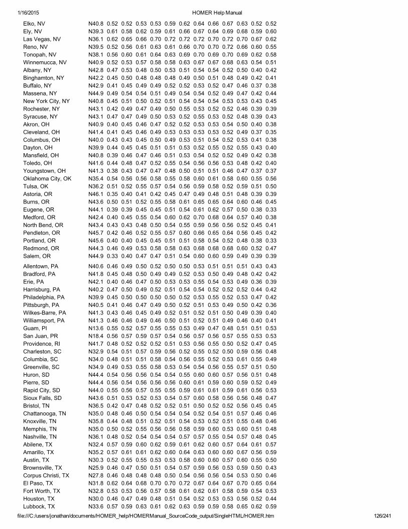
1/16/2015 HOMER Help Manual
file:///C:/users/jonathan/documents/HOMER_help/HOMERManual_SourceCode_output/SingleHTML/HOMER.htm 126/241
Elko, NV N40.8 0.52 0.52 0.53 0.53 0.59 0.62 0.64 0.66 0.67 0.63 0.52 0.52Ely, NV N39.3 0.61 0.58 0.62 0.59 0.61 0.66 0.67 0.64 0.69 0.68 0.59 0.60Las Vegas, NV N36.1 0.62 0.65 0.66 0.70 0.72 0.72 0.72 0.70 0.72 0.70 0.67 0.62Reno, NV N39.5 0.52 0.56 0.61 0.63 0.61 0.66 0.70 0.70 0.72 0.66 0.60 0.55Tonopah, NV N38.1 0.56 0.60 0.61 0.64 0.63 0.69 0.70 0.69 0.70 0.69 0.62 0.58Winnemucca, NV N40.9 0.52 0.53 0.57 0.58 0.58 0.63 0.67 0.67 0.68 0.63 0.54 0.51Albany, NY N42.8 0.47 0.53 0.48 0.50 0.53 0.51 0.54 0.54 0.52 0.50 0.40 0.42Binghamton, NY N42.2 0.45 0.50 0.48 0.48 0.48 0.49 0.50 0.51 0.48 0.49 0.42 0.41Buffalo, NY N42.9 0.41 0.45 0.49 0.49 0.52 0.52 0.53 0.52 0.47 0.46 0.37 0.38Massena, NY N44.9 0.49 0.54 0.54 0.51 0.49 0.54 0.54 0.52 0.49 0.47 0.42 0.44New York City, NY N40.8 0.45 0.51 0.50 0.52 0.51 0.54 0.54 0.54 0.53 0.53 0.43 0.45Rochester, NY N43.1 0.42 0.49 0.47 0.49 0.50 0.55 0.53 0.52 0.52 0.46 0.39 0.39Syracuse, NY N43.1 0.47 0.47 0.49 0.50 0.53 0.52 0.55 0.53 0.52 0.48 0.39 0.43Akron, OH N40.9 0.40 0.45 0.46 0.47 0.52 0.52 0.53 0.53 0.54 0.50 0.40 0.38Cleveland, OH N41.4 0.41 0.45 0.46 0.49 0.53 0.53 0.53 0.53 0.52 0.49 0.37 0.35Columbus, OH N40.0 0.43 0.43 0.45 0.50 0.49 0.53 0.51 0.54 0.52 0.53 0.41 0.38Dayton, OH N39.9 0.44 0.45 0.45 0.51 0.51 0.53 0.52 0.55 0.52 0.55 0.43 0.40Mansfield, OH N40.8 0.39 0.46 0.47 0.46 0.51 0.53 0.54 0.52 0.52 0.49 0.42 0.38Toledo, OH N41.6 0.44 0.48 0.47 0.52 0.55 0.54 0.56 0.56 0.53 0.48 0.42 0.40Youngstown, OH N41.3 0.38 0.43 0.47 0.47 0.48 0.50 0.51 0.51 0.46 0.47 0.37 0.37Oklahoma City, OK N35.4 0.54 0.56 0.56 0.58 0.55 0.58 0.60 0.61 0.58 0.60 0.55 0.56Tulsa, OK N36.2 0.51 0.52 0.55 0.57 0.54 0.56 0.59 0.58 0.52 0.59 0.51 0.50Astoria, OR N46.1 0.35 0.40 0.41 0.42 0.45 0.47 0.49 0.48 0.51 0.48 0.39 0.39Burns, OR N43.6 0.50 0.51 0.52 0.55 0.58 0.61 0.65 0.65 0.64 0.60 0.46 0.45Eugene, OR N44.1 0.39 0.39 0.45 0.45 0.51 0.54 0.61 0.62 0.57 0.50 0.38 0.33Medford, OR N42.4 0.40 0.45 0.55 0.54 0.60 0.62 0.70 0.68 0.64 0.57 0.40 0.38North Bend, OR N43.4 0.43 0.43 0.48 0.50 0.54 0.55 0.59 0.56 0.56 0.52 0.45 0.41Pendleton, OR N45.7 0.42 0.46 0.52 0.55 0.57 0.60 0.66 0.65 0.64 0.56 0.45 0.42Portland, OR N45.6 0.40 0.40 0.45 0.45 0.51 0.51 0.58 0.54 0.52 0.48 0.38 0.33Redmond, OR N44.3 0.46 0.49 0.53 0.58 0.58 0.63 0.68 0.68 0.68 0.60 0.52 0.47Salem, OR N44.9 0.33 0.40 0.47 0.47 0.51 0.54 0.60 0.60 0.59 0.49 0.39 0.39
Allentown, PA N40.6 0.46 0.49 0.50 0.52 0.50 0.50 0.53 0.51 0.51 0.51 0.43 0.43Bradford, PA N41.8 0.45 0.48 0.50 0.49 0.49 0.52 0.53 0.50 0.49 0.48 0.42 0.42Erie, PA N42.1 0.40 0.46 0.47 0.50 0.53 0.53 0.55 0.54 0.53 0.49 0.36 0.39Harrisburg, PA N40.2 0.47 0.50 0.49 0.52 0.51 0.54 0.54 0.52 0.52 0.52 0.44 0.42Philadelphia, PA N39.9 0.45 0.50 0.50 0.50 0.50 0.52 0.53 0.55 0.52 0.53 0.47 0.42Pittsburgh, PA N40.5 0.41 0.46 0.47 0.49 0.50 0.52 0.51 0.53 0.49 0.50 0.42 0.36WilkesBarre, PA N41.3 0.43 0.46 0.45 0.49 0.52 0.51 0.52 0.51 0.50 0.49 0.39 0.40Williamsport, PA N41.3 0.46 0.46 0.49 0.46 0.50 0.51 0.52 0.51 0.49 0.46 0.40 0.41Guam, PI N13.6 0.55 0.52 0.57 0.55 0.55 0.53 0.49 0.47 0.48 0.51 0.51 0.53San Juan, PR N18.4 0.56 0.57 0.59 0.57 0.54 0.56 0.57 0.56 0.57 0.55 0.53 0.53Providence, RI N41.7 0.48 0.52 0.52 0.52 0.51 0.53 0.56 0.55 0.50 0.52 0.47 0.45Charleston, SC N32.9 0.54 0.51 0.57 0.59 0.56 0.52 0.55 0.52 0.50 0.59 0.56 0.48Columbia, SC N34.0 0.48 0.51 0.51 0.58 0.54 0.56 0.55 0.52 0.53 0.61 0.55 0.49Greenville, SC N34.9 0.49 0.53 0.55 0.58 0.53 0.54 0.54 0.56 0.55 0.57 0.51 0.50Huron, SD N44.4 0.54 0.56 0.56 0.54 0.54 0.55 0.60 0.60 0.57 0.56 0.51 0.48Pierre, SD N44.4 0.56 0.54 0.56 0.56 0.56 0.60 0.61 0.59 0.60 0.59 0.52 0.49Rapid City, SD N44.0 0.55 0.56 0.57 0.55 0.55 0.59 0.61 0.61 0.59 0.61 0.56 0.53Sioux Falls, SD N43.6 0.51 0.53 0.52 0.53 0.54 0.57 0.60 0.58 0.56 0.56 0.48 0.47Bristol, TN N36.5 0.42 0.47 0.48 0.52 0.52 0.51 0.50 0.52 0.52 0.56 0.45 0.45Chattanooga, TN N35.0 0.48 0.46 0.50 0.54 0.54 0.54 0.52 0.54 0.51 0.57 0.46 0.46Knoxville, TN N35.8 0.44 0.48 0.51 0.52 0.51 0.54 0.53 0.52 0.51 0.55 0.48 0.46Memphis, TN N35.0 0.50 0.52 0.55 0.56 0.56 0.58 0.59 0.60 0.53 0.60 0.51 0.48Nashville, TN N36.1 0.48 0.52 0.54 0.54 0.54 0.57 0.57 0.55 0.54 0.57 0.48 0.45Abilene, TX N32.4 0.57 0.59 0.60 0.62 0.59 0.61 0.62 0.60 0.57 0.64 0.61 0.57Amarillo, TX N35.2 0.57 0.61 0.61 0.62 0.60 0.64 0.63 0.60 0.60 0.67 0.56 0.59Austin, TX N30.3 0.52 0.55 0.55 0.53 0.53 0.58 0.60 0.60 0.57 0.60 0.55 0.50Brownsville, TX N25.9 0.46 0.47 0.50 0.51 0.54 0.57 0.59 0.56 0.53 0.59 0.50 0.43Corpus Christi, TX N27.8 0.46 0.48 0.48 0.48 0.50 0.54 0.56 0.56 0.54 0.53 0.50 0.46El Paso, TX N31.8 0.62 0.64 0.68 0.70 0.70 0.72 0.67 0.64 0.67 0.70 0.65 0.64Fort Worth, TX N32.8 0.53 0.53 0.56 0.57 0.58 0.61 0.62 0.61 0.58 0.59 0.54 0.53Houston, TX N30.0 0.46 0.47 0.49 0.48 0.51 0.54 0.52 0.53 0.53 0.56 0.52 0.44Lubbock, TX N33.6 0.57 0.59 0.63 0.61 0.62 0.63 0.59 0.59 0.58 0.65 0.62 0.59

1/16/2015 HOMER Help Manual
file:///C:/users/jonathan/documents/HOMER_help/HOMERManual_SourceCode_output/SingleHTML/HOMER.htm 127/241
Lufkin, TX N31.2 0.48 0.50 0.51 0.53 0.55 0.56 0.56 0.57 0.56 0.58 0.54 0.48Midland, TX N31.9 0.60 0.62 0.66 0.64 0.62 0.62 0.65 0.62 0.60 0.65 0.62 0.59Port Arthur, TX N29.9 0.46 0.50 0.51 0.51 0.53 0.58 0.53 0.55 0.54 0.58 0.49 0.47San Angelo, TX N31.4 0.57 0.58 0.59 0.58 0.57 0.60 0.61 0.61 0.59 0.62 0.56 0.56San Antonio, TX N29.5 0.51 0.54 0.55 0.53 0.54 0.58 0.63 0.61 0.58 0.60 0.56 0.51Victoria, TX N28.9 0.47 0.50 0.49 0.49 0.52 0.54 0.57 0.56 0.56 0.56 0.54 0.48Waco, TX N31.6 0.51 0.57 0.54 0.51 0.54 0.60 0.63 0.59 0.58 0.61 0.57 0.53Wichita Falls, TX N34.0 0.55 0.57 0.58 0.58 0.57 0.61 0.62 0.60 0.60 0.60 0.57 0.55Cedar City, UT N37.7 0.58 0.59 0.60 0.63 0.63 0.69 0.65 0.64 0.65 0.68 0.59 0.56Salt Lake City, UT N40.8 0.49 0.54 0.54 0.55 0.62 0.63 0.66 0.67 0.64 0.62 0.54 0.45Lynchburg, VA N37.3 0.50 0.54 0.57 0.55 0.54 0.56 0.57 0.55 0.55 0.55 0.53 0.49Norfolk, VA N36.9 0.50 0.52 0.49 0.53 0.51 0.55 0.52 0.54 0.51 0.55 0.51 0.46Richmond, VA N37.5 0.52 0.51 0.52 0.52 0.52 0.53 0.54 0.52 0.54 0.52 0.50 0.49Roanoke, VA N37.3 0.50 0.51 0.51 0.53 0.54 0.54 0.53 0.53 0.53 0.55 0.51 0.47Sterling, VA N39.0 0.49 0.51 0.51 0.52 0.51 0.54 0.53 0.52 0.53 0.54 0.48 0.42Burlington, VT N44.5 0.50 0.54 0.52 0.51 0.53 0.52 0.53 0.54 0.51 0.48 0.42 0.42Olympia, WA N47.0 0.32 0.39 0.44 0.41 0.46 0.50 0.54 0.54 0.51 0.43 0.36 0.34Quillayute, WA N48.0 0.32 0.36 0.38 0.42 0.46 0.45 0.48 0.46 0.48 0.46 0.36 0.37Seattle, WA N47.5 0.31 0.37 0.44 0.45 0.51 0.52 0.56 0.52 0.52 0.41 0.35 0.29Spokane, WA N47.6 0.49 0.44 0.47 0.51 0.53 0.53 0.65 0.63 0.58 0.55 0.41 0.43Yakima, WA N46.6 0.42 0.50 0.54 0.53 0.58 0.61 0.65 0.63 0.63 0.58 0.44 0.43Eau Claire, WI N44.9 0.50 0.59 0.56 0.49 0.53 0.54 0.54 0.53 0.50 0.49 0.42 0.43Green Bay, WI N44.5 0.49 0.52 0.52 0.52 0.53 0.53 0.56 0.50 0.49 0.50 0.42 0.46
La Crosse, WI N43.9 0.55 0.55 0.53 0.50 0.54 0.53 0.57 0.53 0.50 0.53 0.44 0.43Madison, WI N43.1 0.48 0.54 0.50 0.48 0.54 0.55 0.56 0.57 0.51 0.51 0.44 0.49Milwaukee, WI N43.0 0.51 0.51 0.48 0.51 0.54 0.57 0.54 0.55 0.54 0.51 0.45 0.44Charleston, WV N38.4 0.44 0.44 0.48 0.51 0.50 0.50 0.52 0.52 0.51 0.52 0.45 0.39Elkins, WV N38.9 0.44 0.45 0.45 0.48 0.49 0.49 0.49 0.49 0.48 0.50 0.43 0.39Huntington, WV N38.4 0.46 0.45 0.49 0.49 0.50 0.52 0.51 0.51 0.52 0.52 0.47 0.42Casper, WY N42.9 0.55 0.55 0.56 0.57 0.57 0.61 0.61 0.65 0.62 0.61 0.54 0.51Cheyenne, WY N41.1 0.54 0.56 0.58 0.57 0.56 0.60 0.58 0.59 0.62 0.60 0.57 0.53Lander, WY N42.8 0.57 0.62 0.61 0.59 0.59 0.63 0.63 0.62 0.66 0.63 0.59 0.58Rock Springs, WY N41.6 0.53 0.56 0.58 0.60 0.60 0.62 0.64 0.65 0.65 0.64 0.54 0.52Sheridan, WY N44.8 0.55 0.55 0.56 0.55 0.52 0.58 0.60 0.62 0.61 0.58 0.54 0.53
For more informationThe HOMER Support Site has a searchable knowledgebase and additional support options.
HOMER online contains the latest information on model updates, as well as sample files, resource data, and contact information.
© 20122014 HOMER Energy, LLCLast modified: Sept 28, 2012
[TOP]
4.3 Wind Data Histograms
Wind Data Histograms
The following five wind data parameters were measured for the 239 weather stations in the U.S. National Solar Radiation Data Base:
annual average wind speedWeibull k valueautocorrelation factordiurnal pattern strengthhour of peak wind speed
The numerical results are displayed in the table of measured parameters. The histograms below show the distribution of each of these parameters:
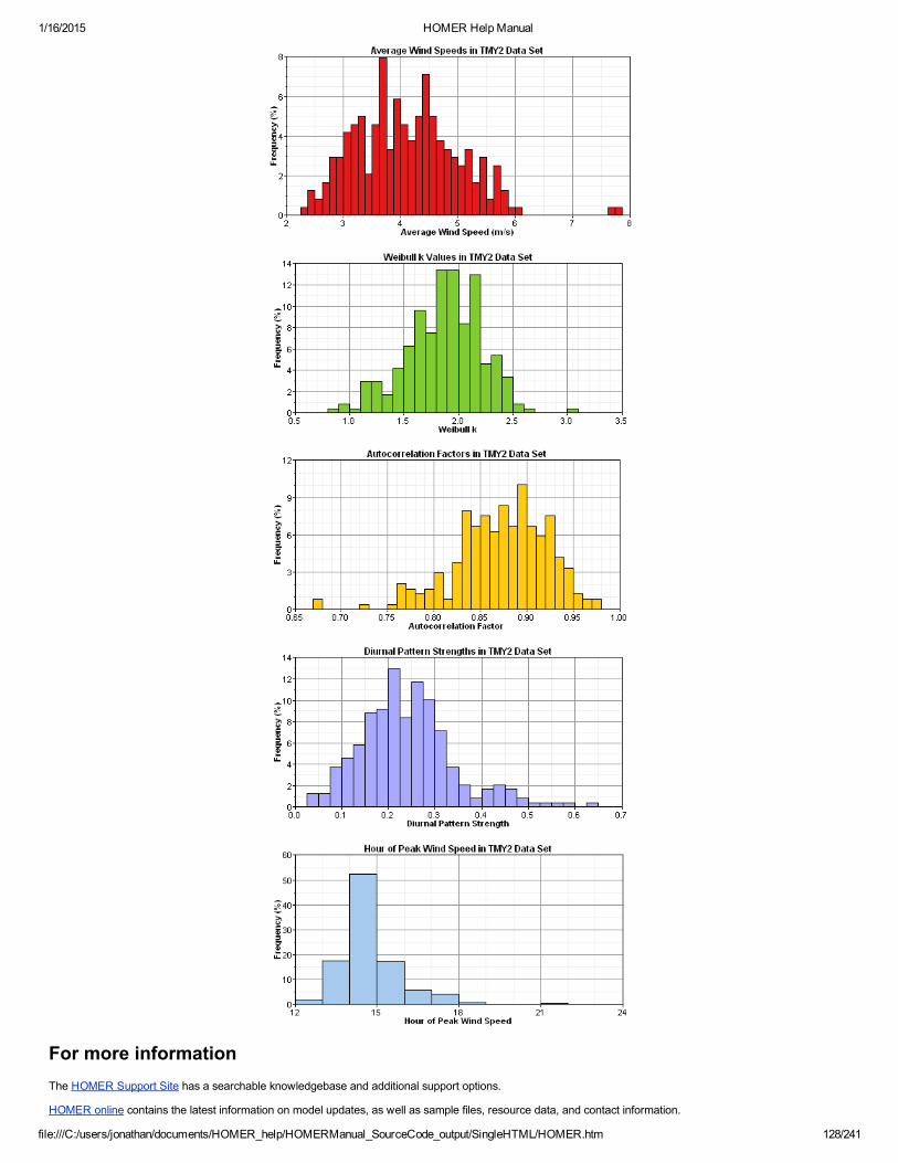
1/16/2015 HOMER Help Manual
file:///C:/users/jonathan/documents/HOMER_help/HOMERManual_SourceCode_output/SingleHTML/HOMER.htm 128/241
For more informationThe HOMER Support Site has a searchable knowledgebase and additional support options.
HOMER online contains the latest information on model updates, as well as sample files, resource data, and contact information.

1/16/2015 HOMER Help Manual
file:///C:/users/jonathan/documents/HOMER_help/HOMERManual_SourceCode_output/SingleHTML/HOMER.htm 129/241
© 20122014 HOMER Energy, LLCLast modified: Sept 28, 2012
[TOP]
4.4 Wind Data Parameters
Wind Data Parameters
The following table contains the following parameters for each of the 239 stations in the US National Solar Radiation Data Base:
annual average wind speed, vave [m/s]Weibull k value, konehour autocorrelation factor, r1diurnal pattern strength, dhour of peak wind speed, f
You can also look at histograms of these parameters.
Important: The stations that make these measurements are not typically located so as to maximize the wind resource. So this data is likely to be conservative interms of wind speed, since in siting a wind turbine you would normally seek out a ridgeline or other topographic feature to maximize average wind speeds. Also,this data is compiled from TMY (Typical Meteorological Year) data, which is chosen as "typical" largely on the basis of solar data, not wind data. So these data donot necessarily represent a typical year of wind speeds.
City State vave k r1 d fAnchorage AK 3.277 1.681 0.769 0.125 17Annette AK 4.206 1.650 0.973 0.132 13Barrow AK 5.482 2.234 0.948 0.036 15Bethel AK 5.659 2.166 0.950 0.059 16Bettles AK 3.148 1.689 0.873 0.112 14Big Delta AK 4.069 1.297 0.966 0.091 17Cold Bay AK 7.661 2.019 0.913 0.075 15Fairbanks AK 2.506 1.289 0.787 0.160 17Gulkana AK 2.651 0.809 0.934 0.183 16King Salmon AK 4.882 1.874 0.932 0.143 16Kodiak AK 4.652 1.468 0.895 0.082 15Kotzebue AK 6.005 1.833 0.934 0.030 14McGrath AK 2.482 1.428 0.894 0.202 16Nome AK 4.774 1.621 0.920 0.117 15St. Paul Island AK 7.802 2.084 0.966 0.052 14Talkeetna AK 2.465 1.030 0.876 0.268 15Yakutat AK 2.964 1.359 0.945 0.218 14Birmingham AL 3.163 1.521 0.831 0.345 13Huntsville AL 3.626 1.619 0.838 0.276 13Mobile AL 3.684 1.852 0.849 0.268 13Montgomery AL 3.023 1.658 0.794 0.338 13Fort Smith AR 3.235 1.845 0.901 0.307 14Little Rock AR 3.435 1.887 0.807 0.284 14Flagstaff AZ 3.238 1.537 0.922 0.447 14Phoenix AZ 2.984 2.016 0.727 0.148 14Prescott AZ 3.734 1.927 0.847 0.272 15Tucson AZ 3.935 2.127 0.858 0.160 15Arcata CA 3.051 1.366 0.911 0.424 14Bakersfield CA 2.852 1.750 0.830 0.267 16Dagget CA 4.901 1.750 0.933 0.028 21Fresno CA 2.986 1.880 0.867 0.194 17Long Beach CA 2.702 1.595 0.850 0.549 15Los Angeles CA 3.575 1.961 0.676 0.469 15Sacramento CA 3.251 1.413 0.894 0.276 15San Diego CA 3.224 1.983 0.798 0.412 14San Francisco CA 4.530 1.689 0.876 0.405 17Santa Maria CA 3.356 1.271 0.871 0.632 15Alamosa CO 3.746 1.502 0.900 0.336 17Boulder/Denver CO 3.639 1.849 0.678 0.208 16

1/16/2015 HOMER Help Manual
file:///C:/users/jonathan/documents/HOMER_help/HOMERManual_SourceCode_output/SingleHTML/HOMER.htm 130/241
Colorado Springs CO 4.356 1.890 0.831 0.185 15Eagle CO 2.712 0.944 0.836 0.579 16Grand Junction CO 3.560 1.784 0.823 0.086 14Pueblo CO 4.097 1.678 0.842 0.311 16Bridgeport CT 5.423 2.336 0.880 0.173 14Hartford CT 3.831 1.878 0.882 0.275 14Wilmington DE 4.134 1.977 0.899 0.252 14Daytona Beach FL 3.811 1.795 0.895 0.416 14Jacksonville FL 3.283 1.555 0.775 0.463 14Key West FL 5.089 2.506 0.942 0.069 13Miami FL 4.337 2.214 0.803 0.292 14Tallahassee FL 2.901 1.432 0.841 0.460 14Tampa FL 3.579 2.147 0.762 0.336 14West Palm Beach FL 4.391 1.984 0.926 0.297 14Athens GA 3.314 2.002 0.920 0.209 14Atlanta GA 3.947 2.152 0.808 0.170 14Augusta GA 3.158 1.587 0.860 0.338 14Columbus GA 2.950 1.604 0.889 0.346 14Macon GA 3.287 1.689 0.780 0.307 14Savannah GA 3.565 1.969 0.918 0.324 14Hilo HI 3.142 2.263 0.839 0.260 14Honolulu HI 4.950 2.433 0.822 0.306 15Kahului HI 5.712 2.305 0.880 0.374 15Lihue HI 5.503 3.024 0.951 0.086 15Des Moines IA 4.696 1.999 0.922 0.216 13Mason City IA 5.079 2.052 0.898 0.210 13Sioux City IA 4.885 2.030 0.894 0.208 14Waterloo IA 4.763 1.904 0.897 0.235 13Boise ID 3.810 1.845 0.779 0.201 15Pocatello ID 4.728 1.731 0.881 0.192 15Chicago IL 4.620 2.152 0.847 0.195 14Moline IL 4.619 1.896 0.905 0.260 13Peoria IL 4.379 2.124 0.859 0.224 13Rockford IL 4.665 2.137 0.903 0.234 13Springfield IL 4.804 2.178 0.909 0.159 13Evansville IN 3.525 1.492 0.858 0.327 13Fort Wayne IN 4.468 2.115 0.899 0.200 14Indianapolis IN 4.063 1.966 0.890 0.209 14South Bend IN 4.503 2.084 0.894 0.225 14Dodge City KS 5.790 2.404 0.847 0.130 13Goodland KS 5.831 2.396 0.855 0.084 13Topeka KS 4.392 1.843 0.847 0.249 14
Wichita KS 5.214 2.205 0.909 0.175 14Covington KY 3.950 2.076 0.856 0.207 14Lexington KY 3.942 2.277 0.929 0.180 13Louisville KY 3.672 1.876 0.831 0.268 15Baton Rouge LA 3.239 1.647 0.872 0.311 14Lake Charles LA 3.775 1.973 0.832 0.286 14New Orleans LA 3.582 1.828 0.864 0.258 13Shreveport LA 3.464 1.746 0.841 0.279 14Boston MA 5.430 2.401 0.838 0.126 14Worcester MA 4.319 1.944 0.903 0.087 13Baltimore MD 4.108 1.995 0.842 0.264 14Caribou ME 4.593 1.769 0.909 0.172 14Portland ME 3.904 1.908 0.856 0.295 14Alpena MI 3.693 1.943 0.897 0.289 14Detroit MI 4.507 2.123 0.848 0.243 14Flint MI 4.378 2.027 0.886 0.212 14Grand Rapids MI 4.454 2.199 0.892 0.215 14Houghton MI 4.060 2.338 0.909 0.161 15Lansing MI 4.344 1.855 0.933 0.223 14Muskegon MI 4.888 2.104 0.931 0.190 14

1/16/2015 HOMER Help Manual
file:///C:/users/jonathan/documents/HOMER_help/HOMERManual_SourceCode_output/SingleHTML/HOMER.htm 131/241
Sault Ste. Marie MI 3.806 1.987 0.862 0.244 15Traverse City MI 3.993 1.818 0.868 0.241 14Duluth MN 4.701 2.205 0.924 0.156 14International Falls MN 4.019 1.977 0.871 0.221 13Minneapolis/St. Paul MN 4.624 2.016 0.897 0.223 14Rochester MN 5.789 2.441 0.926 0.130 12St. Cloud MN 3.661 1.730 0.942 0.274 14Columbia MO 4.439 2.322 0.874 0.157 13Kansas City MO 4.482 2.527 0.842 0.166 14Springfield MO 4.506 2.284 0.858 0.190 12St. Louis MO 4.401 2.094 0.857 0.172 14Jackson MS 3.322 1.607 0.857 0.324 13Meridian MS 2.769 1.247 0.825 0.434 13Billings MT 5.155 2.324 0.885 0.079 14Cut Bank MT 5.672 1.761 0.946 0.225 15Glasgow MT 4.802 2.059 0.933 0.130 14Great Falls MT 5.513 1.898 0.906 0.156 14Helena MT 3.527 1.537 0.876 0.281 16Kalispell MT 2.828 1.139 0.905 0.255 14Lewistown MT 4.245 1.745 0.917 0.149 14Miles City MT 4.624 2.040 0.836 0.102 14
Missoula MT 3.023 1.296 0.831 0.327 17
Asheville NC 3.480 1.308 0.854 0.313 14Cape Hatteras NC 5.157 2.419 0.954 0.100 14Charlotte NC 3.139 1.825 0.791 0.291 14Greensboro NC 3.116 1.861 0.823 0.287 13Raleigh/Durham NC 3.503 2.005 0.816 0.245 14Wilmington NC 3.670 1.822 0.904 0.309 14Bismarck ND 4.420 1.608 0.875 0.308 14Fargo ND 5.377 2.026 0.927 0.158 14Minot ND 5.489 2.310 0.879 0.138 14Grand Island NE 5.336 2.246 0.910 0.175 14Norfolk NE 5.455 1.710 0.924 0.229 14North Platte NE 4.651 1.692 0.862 0.264 15Omaha NE 4.493 1.838 0.922 0.176 13Scottsbluff NE 4.663 1.820 0.813 0.235 14Concord NH 2.865 1.149 0.838 0.441 14Atlantic City NJ 4.420 1.935 0.948 0.262 14Newark NJ 4.624 2.345 0.809 0.157 15Albuquerque NM 4.009 1.723 0.789 0.255 17Tucumcari NM 4.335 1.907 0.911 0.208 14Elko NV 2.700 1.195 0.827 0.470 15Ely NV 4.374 1.963 0.879 0.078 13Las Vegas NV 4.063 1.809 0.854 0.139 18Reno NV 2.839 1.124 0.856 0.555 17Tonopah NV 4.317 1.804 0.826 0.167 15Winnemucca NV 3.630 1.833 0.851 0.245 15Albany NY 3.958 1.567 0.856 0.259 14Binghamton NY 4.509 2.357 0.891 0.155 14Buffalo NY 5.135 2.152 0.889 0.181 14Massena NY 3.632 1.520 0.885 0.267 13NYC (Central Park) NY 5.185 2.676 0.933 0.130 15Rochester NY 4.377 1.983 0.916 0.183 14Syracuse NY 4.100 1.903 0.877 0.202 14Akron/Canton OH 4.173 2.179 0.890 0.210 13Cleveland OH 4.506 2.186 0.842 0.191 14Columbus OH 3.728 1.898 0.847 0.288 14Dayton OH 4.311 2.106 0.847 0.185 14Mansfield OH 4.786 2.342 0.930 0.159 13Toledo OH 4.150 1.914 0.898 0.266 14Youngstown OH 4.407 2.312 0.893 0.178 14Oklahoma City OK 5.352 2.253 0.937 0.183 13

1/16/2015 HOMER Help Manual
file:///C:/users/jonathan/documents/HOMER_help/HOMERManual_SourceCode_output/SingleHTML/HOMER.htm 132/241
Tulsa OK 4.811 2.173 0.902 0.222 14Astoria OR 3.987 1.876 0.916 0.254 15Burns OR 3.213 1.652 0.946 0.240 15Eugene OR 3.366 1.904 0.890 0.273 14Medford OR 2.255 1.262 0.765 0.484 16North Bend OR 4.276 1.768 0.911 0.322 15Pendleton OR 3.826 1.749 0.885 0.125 16Portland OR 3.580 1.560 0.872 0.230 16Redmond/Bend OR 3.640 1.913 0.835 0.295 15Salem OR 3.127 1.387 0.897 0.291 14Allentown PA 4.143 1.684 0.884 0.289 14Bradford PA 3.660 1.765 0.921 0.260 14Erie PA 5.141 2.216 0.910 0.104 12Harrisburg PA 3.353 1.513 0.845 0.278 14Philadelphia PA 4.307 2.190 0.831 0.203 14Pittsburgh PA 3.922 1.760 0.850 0.284 14WilkesBarre PA 3.641 2.146 0.836 0.222 14Williamsport PA 3.442 1.295 0.870 0.297 14Guam PI 4.205 2.189 0.973 0.307 13San Juan PR 3.823 1.788 0.869 0.504 15Providence RI 4.702 2.157 0.881 0.257 14Charleston SC 3.892 2.069 0.821 0.318 14Columbia SC 3.035 1.555 0.773 0.382 14Greenville SC 2.982 1.810 0.896 0.277 13Huron SD 4.842 1.956 0.918 0.202 14Pierre SD 5.102 1.884 0.920 0.194 14Rapid City SD 5.342 1.677 0.928 0.231 13Sioux Falls SD 5.023 2.021 0.927 0.217 14Bristol TN 2.397 1.174 0.833 0.437 15Chattanooga TN 2.507 1.108 0.801 0.493 15Knoxville TN 3.023 1.545 0.845 0.262 15Memphis TN 3.998 1.903 0.887 0.229 13Nashville TN 3.642 1.902 0.803 0.250 14Abilene TX 5.205 2.418 0.915 0.119 14Amarillo TX 5.929 2.411 0.878 0.129 14Austin TX 4.062 1.895 0.835 0.238 14Brownsville TX 5.266 2.130 0.924 0.361 14Corpus Christi TX 5.377 2.197 0.918 0.303 15El Paso TX 3.534 1.612 0.798 0.241 16Fort Worth TX 4.433 1.984 0.909 0.191 14Houston TX 3.777 2.112 0.775 0.321 14
Lubbock TX 5.196 2.164 0.890 0.184 15Lufkin TX 3.068 1.515 0.854 0.395 14
Midland/Odessa TX 5.050 2.184 0.832 0.225 14Port Arthur TX 4.367 2.176 0.885 0.261 14San Angelo TX 4.638 2.150 0.863 0.199 14San Antonio TX 4.200 2.332 0.864 0.202 15Victoria TX 4.487 2.158 0.929 0.308 14Waco TX 4.842 2.323 0.906 0.138 14Wichita Falls TX 5.675 2.414 0.944 0.164 14Cedar City UT 3.554 1.179 0.861 0.439 16Salt Lake City UT 3.968 1.667 0.762 0.119 13Lynchburg VA 3.061 1.454 0.867 0.359 14Norfolk VA 4.883 2.207 0.862 0.183 13Richmond VA 3.653 2.110 0.897 0.227 14Roanoke VA 3.630 1.662 0.859 0.265 15Sterling VA 3.490 1.694 0.821 0.291 14Burlington VT 4.064 2.004 0.806 0.204 13Olympia WA 3.060 1.441 0.883 0.303 14Quillayute WA 2.787 1.559 0.871 0.372 14Seattle WA 3.897 2.108 0.760 0.121 15Spokane WA 4.333 1.934 0.875 0.122 12
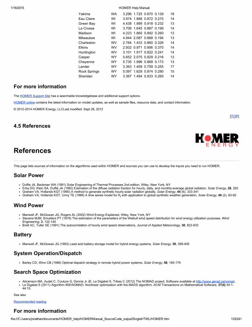
1/16/2015 HOMER Help Manual
file:///C:/users/jonathan/documents/HOMER_help/HOMERManual_SourceCode_output/SingleHTML/HOMER.htm 133/241
Yakima WA 3.296 1.725 0.870 0.139 18Eau Claire WI 3.974 1.888 0.872 0.275 14Green Bay WI 4.438 1.999 0.918 0.232 13La Crosse WI 3.706 1.645 0.887 0.199 14Madison WI 4.223 1.860 0.892 0.260 13Milwaukee WI 4.944 2.087 0.868 0.194 13Charleston WV 2.764 1.433 0.860 0.326 14Elkins WV 2.932 0.971 0.906 0.370 14Huntington WV 3.101 1.917 0.822 0.241 14Casper WY 5.652 2.075 0.929 0.216 13Cheyenne WY 5.735 1.996 0.868 0.173 13Lander WY 3.363 1.459 0.759 0.255 17Rock Springs WY 5.097 1.629 0.874 0.280 15Sheridan WY 3.367 1.494 0.833 0.265 14
For more informationThe HOMER Support Site has a searchable knowledgebase and additional support options.
HOMER online contains the latest information on model updates, as well as sample files, resource data, and contact information.
© 20122014 HOMER Energy, LLCLast modified: Sept 28, 2012
[TOP]
4.5 References
References
This page lists sources of information on the algorithms used within HOMER and sources you can use to develop the inputs you need to run HOMER.
Solar PowerDuffie JA, Beckman WA (1991) Solar Engineering of Thermal Processes 2nd edition, Wiley, New York, NYErbs DG, Klein SA, Duffie JA (1982) Estimation of the diffuse radiation fraction for hourly, daily, and monthlyaverage global radiation, Solar Energy, 28, 293Graham VA, Hollands KGT (1990) A method to generate synthetic hourly solar radiation globally, Solar Energy, 44 (6), 333341Graham VA, Hollands KGT, Unny TE (1988) A time series model for Kt with application to global synthetic weather generation, Solar Energy, 40 (2), 8392
Wind PowerManwell JF, McGowan JG, Rogers AL (2002) Wind Energy Explained, Wiley, New York, NYStevens MJM, Smulders PT (1979) The estimation of the parameters of the Weibull wind speed distribution for wind energy utilization purposes, WindEngineering, 3, 132145Brett AC, Tuller SE (1991) The autocorrelation of hourly wind speed observations, Journal of Applied Meteorology, 30, 823833
BatteryManwell JF, McGowan JG (1993) Lead acid battery storage model for hybrid energy systems, Solar Energy, 50, 399405
System Operation/DispatchBarley CD, Winn CB (1996) Optimal dispatch strategy in remote hybrid power systems, Solar Energy, 58, 165179
Search Space OptimizationAbramson MA, Audet C, Couture G, Dennis Jr JE, Le Digabel S, Tribes C (2012) The NOMAD project, Software available at http://www.gerad.ca/nomad .Le Digabel S (2011) Algorithm 909:NOMAD: Nonlinear optimization with the MADS algorithm, ACM Transactions on Mathematical Software, 37(4) 44:144:15.
See also
Recommended reading
For more information

1/16/2015 HOMER Help Manual
file:///C:/users/jonathan/documents/HOMER_help/HOMERManual_SourceCode_output/SingleHTML/HOMER.htm 134/241
The HOMER Support Site has a searchable knowledgebase and additional support options.
HOMER online contains the latest information on model updates, as well as sample files, resource data, and contact information.
© 20122014 HOMER Energy, LLCLast modified: July 28, 2004
[TOP]
4.6 Recommended Reading
Recommended Reading
This page lists sources of information that you might find helpful in learning about micropower systems. None of this information is essential to running HOMER.
Renewable and Micropower SystemsMasters G (2004) Renewable and Efficient Electric Power Systems, WileyIEEE Press, ISBN: 0471280607Borbely AM, Kreider JF, (2001) Distributed Generation: The Power Paradigm for the New Millennium, CRC Press, ISBN: 0849300746
Solar ResourceChapters 1 and 2 of Duffie JA, Beckman WA (1991) Solar Engineering of Thermal Processes 2nd edition, Wiley, New York, NY, ISBN: 0471510564
Wind ResourceAn excellent and multilingual source of information on the wind resource, wind turbine technology, economics and more is www.windpower.org, the DanishWind Industry Association's website.Chapter 2 of Manwell JF, McGowan JG, Rogers AL (2002) Wind Energy Explained, Wiley, New York, NY, ISBN: 0471499722
Biomass ResourceMcKendry P (2002a) Energy production from biomass (part 1): overview of biomass, Bioresource Technology, 83, 3746
Biomass PowerMcKendry P (2002b) Energy production from biomass (part 2): conversion technologies, Bioresource Technology, 83, 4754
Hydro PowerFor a helpful introduction to small hydro, see Paish O (2002) Small hydro power: technology and current status, Renewable and Sustainable EnergyReviews, 6, 537556For a useful website on all things microhydro, see www.microhydropower.net.Some useful calculation tools are available at the website of VA Tech Hydro, www.compacthydro.com.
See also
References
For more informationThe HOMER Support Site has a searchable knowledgebase and additional support options.
HOMER online contains the latest information on model updates, as well as sample files, resource data, and contact information.
© 20122014 HOMER Energy, LLCLast modified: September 9, 2004
[TOP]
5. License Management
License Management
License info can be found under the Help tab in the navigation bar at the top of the HOMER window.This window shows you the status of your HOMER license,provides a link to the webpage where you can renew your license, and lets you import the license renewal file that the webpage sends you.

1/16/2015 HOMER Help Manual
file:///C:/users/jonathan/documents/HOMER_help/HOMERManual_SourceCode_output/SingleHTML/HOMER.htm 135/241
See also
Renewing your HOMER license
For more informationThe HOMER Support Site has a searchable knowledgebase and additional support options.
HOMER online contains the latest information on model updates, as well as sample files, resource data, and contact information.
© 20122014 HOMER Energy, LLCLast modified: April 21, 2010
[TOP]
6. Glossary
6.1 EnglishSpanish Glossary
EnglishSpanish Glossary
This glossary includes words and terms that are part of the HOMER user interface with their equivalents in Spanish. The words appear in alphabetical order, basedon the English spelling.
To see a definition, click on a letter below to go to the section of the glossary for that letter.
A B C D E F G H I J K L M N O P Q R S T U V W X Y Z
English Spanish
Agregar/Eliminar A
Abbreviation Abreviación
AC CA
Add noise Agregar ruido
Add/Remove
Advanced parameters Parámetros avanzados
Allow multiple generatorsto operate simultaneously Permite múltiples generadores para operar simultáneamente
Allow systems with generatorcapacity less than peak load Permite sistemas con generadores de capacidad inferior a picos de demanda
Allow systems with multiplegenerators Permite sistemas con múltiples generadores
Annual electric energy production Producción anual de energía eléctrica
Annual electric loads Cargas eléctricas anuales
Annual fuel consumption Consumo anual de combustible
Annual peak Pico anual
Annual peak load Carga anual pico
Annual real interest rate Tasa de interés real anual
Apply setpoint SOC Aplica punto de ajuste EDC (Estado De Carga)
As percent of load Como porcentaje de la carga
As percent of renewable output Como porcentaje de producción renovable
Author Autor
Autocorrelation factor Factor de auto corrección
Automatically check forupdates on startup Revisa automáticamente para actualizarse al inicio
Available biomass Biomasa disponible
Average electrical efficiency Eficiencia eléctrica promedio

1/16/2015 HOMER Help Manual
file:///C:/users/jonathan/documents/HOMER_help/HOMERManual_SourceCode_output/SingleHTML/HOMER.htm 136/241
Average electrical output Producción eléctrica promedio
Average Hydrogen Load Carga promedio de hidrógeno
Average price Precio promedio
Average total efficiency Promedio de eficiencia total
Azimuth Azimut B
Baseline data Datos base
Batt. (battery) Batería
Batt. cap. mult. Multiplicador del costo inversión de la batería
Batt. capital cost Multiplier Multiplicador del costo inversión de la batería
Batt. O&M mult. Multiplicador del costo operación y mantenimiento de la batería
Batt. O&M cost multiplier Multiplicador del costo operación y mantenimiento de la batería
Batt. repl. mult. Multiplicador del costo reemplazo batería
Batt. replacement cost multiplier Multiplicador del costo reemplazo de la batería
Battery Batería
Battery capital cost multiplier Multiplicador del costo inversión de la batería
Battery O&M cost multiplier Multiplicador del costo operación y mantenimiento de la batería
Battery replacement costmultiplier Multiplicador del costo reemplazo de la batería
Bio. gas. ratio Razón de biogás
Bio. GR Razón de biogás
Biogas Biogás
Biogas LHV Valor calórico mas bajo de biogás (VCB)
Biogas lower heating value Valor calórico mas bajo de biogás
Biomass carbon content Contenido de carbón biomasa
Biomass data scaled average Promedio escalado de datos de biomasa
Biomass gasification ratio Razón de gasificación de la biomasa
Biomass price Precio de la biomasa
Biomass resource Recurso de biomasa
Biomass resource price Precio del recurso biomasa
Boiler Calentador
Boiler cap. Capacidad de la caldera
Boiler capacity Capacidad de la caldera
Boiler eff. Eficiencia de la caldera
Boiler efficiency Eficiencia de la caldera C
Calculate Calcular
Calculated parameters Parámetros calculados
Cancel Cancelar
Capacity curve Curva de capacidad
Capacity ratio Razón de capacidad
Capacity relative to inverter Capacidad relativa al inversor
Capacity shortage Falta de capacidad
Capital Capital
Carbon content Contenido de carbón
Carbon emissions Emisiones de carbón
Clear Borrar
Clearness index Índice de claridad
COE (cost of energy) CE (costo de la energía)
Cofire inputs Datos del combustible alterno

1/16/2015 HOMER Help Manual
file:///C:/users/jonathan/documents/HOMER_help/HOMERManual_SourceCode_output/SingleHTML/HOMER.htm 137/241
Cofire with biogas Combustible con biogás
Component Componente
Constraints Consideraciones
Consumption limit Limite de consumo
Conv. (converter) Convertidor
Conv. cap. mult. Multiplicador del costo inversión del convertidor
Conv. O&M mult. Multiplicador del costo operación y mantenimiento del convertidor
Conv. repl. mult. Multiplicador del costo reemplazo del convertidor
Converter Convertidor
Converter capital cost multiplier Multiplicador del costo inversión del convertidor
Converter capital multiplier Multiplicador del costo inversión del convertidor
Converter O&M cost multiplier Multiplicador del costo operación y mantenimiento del convertidor
Converter O&M multiplier Multiplicador del costo operación y mantenimiento del convertidor
Converter replacementcost multiplier Multiplicador del costo reemplazo del convertidor
Converter replacementmultiplier Multiplicador del costo reemplazo del convertidor
Cost curve Curva de costo
Costs Costos
Current Corriente
Cycle charging Ciclos de carga
Cycles to failure Ciclos de falla D
Daily noise Ruido diario
Daily radiation Radiación diaria
Day type Tipo de día
DC CD
Default author Autor por definición
Def. load min. Carga Mínima diferida
Def. load peak Carga Pico diferida
Def. load storage Capacidad de almacenamiento diferida
Deferrable load Cargas diferidas
Deferrable load min. Carga mínima diferida
Deferrable load minimum Carga mínima diferida
Deferrable load peak Carga pico diferida
Deferrable load served Cargas diferidas servidas
Deferrable load storagecapacity Capacidad de almacenamiento diferida
Degrees Grados
Delete Eliminar
Demand Demanda
Demand rate Razón de demanda
Density Densidad
Depth of discharge Profundidad de descarga
Derating factor Factor de reducción
Design flow rate Razón de flujo de diseño
Details Detalles
Dispatch strategy Estrategia de despacho
Diurnal pattern strength Patrón diurno de intensidad
Document Documento E

1/16/2015 HOMER Help Manual
file:///C:/users/jonathan/documents/HOMER_help/HOMERManual_SourceCode_output/SingleHTML/HOMER.htm 138/241
Economics Económicos
Efficiency curve Curva de eficiencia
Efficiency inputs Datos de eficiencia
Elec. (electrolyzer) Elec. (fluido electrolítico)
Elec. cap. mult. Multiplicador del costo inversión del electrolizador
Elec. eff. Eficiencia electrolizador
Elec. min. Mínimo electrolizador
Elec. min. load Carga mínima electrolizador
Elec. O&M mult. Multiplicador del costo operación y mantenimiento del electrolizador
Elec. repl. mult. Multiplicador del costo reemplazo del electrolizador
Electrolyzer Fluido electrolítico
Electrolyzer capital costmultiplier Multiplicador del costo de inversión del electrolizador
Electrolyzer capital multiplier Multiplicador del costo de inversión del electrolizador
Electrolyzer eff. Eficiencia electrolítica
Electrolyzer efficiency Eficiencia electrolítica
Electrolyzer life Vida del electrolito
Electrolyzer lifetime Tiempo de vida del electrolito
Electrolyzer load served Cargas cubiertas por el electrolizador
Electrolyzer minimum loadratio Razón carga mínima del electrolizador
Electrolyzer O&M cost multiplier Multiplicador del costo operación y mantenimiento del electrolizador
Electrolyzer O&M multiplier Multiplicador del costo operación y mantenimiento del electrolizador
Electrolyzer replacement cost multiplier Multiplicador del costo reemplazo del electrolizador
Electrolyzer replacement multiplier Multiplicador del costo reemplazo del electrolizador
Equipment to consider Equipo a considerar
Excess electricity Excedente de electricidad
Excess electricity can serve thermal load Excedente de electricidad puede servir a cargas térmicas
Export Exportar F
File version Versión del archivo
Fixed (variables) Fijo (variables)
Fixed cap. cost Costo de inversión fijo
Fixed O&M cost Costo de operación y mantenimiento fijo
Fuel curve Curva de combustible G
Generator Generador
Generator control Control del generador
Generator fuel curve intercept coefficient Coeficiente de intercepción de la curva de combustible del generador
Generator fuel curve slope Pendiente de la curva de combustible del generador
Generator heat recovery ratio Razón de recuperación de calor generador
Generator lifetime Tiempo de vida generador
Generator minimum fossilfraction Fracción combustible mínimo generador
Generator minimum load Carga mínima generador
Generator substitution ratio Razón de sustitución generador
Generator type Tipo de generador

1/16/2015 HOMER Help Manual
file:///C:/users/jonathan/documents/HOMER_help/HOMERManual_SourceCode_output/SingleHTML/HOMER.htm 139/241
Global solar Radiación solar globalGraphic Grafica
Grid Red
Grid cap. Capacidad de la red
Grid capital cost Costo de la red
Grid demand rate Razón de demanda de la red
Grid extension cost Costo extensión de la red
Grid extension capital cost Costo por extensión de la red
Grid extension O&M Cost Costo por operación y mantenimiento de extensión de la red
Grid extension power price Precio de la energía por extensión de la red
Grid interconnection charge Cargo por interconexión con la Red
Grid O&M Costo por operación y mantenimiento de la red
Grid O&M cost Costo por operación y mantenimiento de la red
Grid power Capacidad de la red
Grid power price Precio de la energía de la red
Grid power price Precio de la energía de la red
Grid sellback rate Razón de repago de la red
Grid standby charge Cargo por tiempo de espera de la red
Gridconnected system Sistema conectado a la red
Grnd. ref. Reflexión de tierra
Ground reflectance Reflexión de tierra H
H2 Load Carga hidrogeno
H2 tank capital multiplier Multiplicador del costo inversión del tanque de hidrogeno
H2 tank life Tiempo de vida del tanque de hidrogeno
H2 tank O&M multiplier Multiplicador del costo de operación y mantenimiento del tanque de hidrogeno
H2 tank replacement multiplier Multiplicador de reemplazo del tanque de Hidrogeno
Help Ayuda
Hour of peak wind speed Hora de velocidad de viento pico
Hourly data Datos horarios
Hourly load Carga horaria
Hourly noise Ruido horario
Hours of operations Horas de operación
HT cap. mult. Multiplicador del costo inversión del tanque de hidrogeno
HT O&M mult. Multiplicador del costo de operación y mantenimiento del tanque de hidrogeno
HT repl. mult. Multiplicador del costo de reemplazo del tanque de Hidrogeno
Hydro Hidroeléctrica
Hydro capital Costo de la hidroeléctrica
Hydro capital Cost Costo de la hidroeléctrica
Hydro data scaled Average Promedio de datos escalados de hidro
Hydro design Flow Rate Tasa de flujo de diseño de la hidro
Hydro eff. Eficiencia de la Hidro
Hydro head Carga (Salto) de la hidro
Hydro head loss Perdida de carga de la hidro
Hydro life Vida de la hidro
Hydro lifetime Tiempo de vida de la hidro
Hydro maximum flow ratio Tasa de flujo máximo de la hidro
Hydro minimum flow ratio Tasa de flujo mínimo de la hidro
Hydro O&M operación y mantenimiento de la hidro
1/16/2015 HOMER Help Manual
file:///C:/users/jonathan/documents/HOMER_help/HOMERManual_SourceCode_output/SingleHTML/HOMER.htm 140/241
Hydro O&M cost Costo de operación y mantenimiento de la hidroHydro repl. Reemplazo de la hidro
Hydro replacement Reemplazo de la hidro
Hydro replacement cost Costo del reemplazo de la hidro
Hydro resource Recurso hidráulico
Hydro turbine efficiency Eficiencia de la turbina hidro
Hydrogen load Carga de hidrógeno
Hydrogen tank capital cost multiplier Multiplicador del costo inversión del tanque del hidrógeno
Hydrogen tank lifetime Tiempo de vida del tanque de hidrógeno
Hydrogen tank O&M cost multiplier Multiplicador del costo de operación y mantenimiento del tanque de hidrógeno
Hydrogen tank replacementcost multiplier Multiplicador del costo de reemplazo del tanque de hidrógeno
Hydrogen consumption Consumo de hidrógeno I
Import file Importar archivo
Intake pipe Tubo de admisión
Intercept Interceptar
Interconn. charge Cargo por interconexión
Interconnection charge Cargo por interconexión
Interest rate Tasa de interés
Inverter Inversor
Inverter eff. Eficiencia del inversor
Inverter efficiency Eficiencia del inversor
Inverter life Vida del inversor
Inverter lifetime Tiempo de vida del inversor J
K
L
Label Etiqueta
Latitude Latitud
Legend Leyenda
LHV of biogas Valor calórico bajo del biogás
Lifetime Tiempo de vida
Lifetime curve Curva de tiempo de vida
Lifetime throughput Rendimiento en el tiempo de vida
Limit consumption to Limite de consumo para
Link with Enlace con
Load Carga
Load factor Factor de carga
Load following Seguimiento de la carga
Load profile Perfil de carga
Load type Tipo de carga
Longitude Longitud
Lower heating value Valor calórico bajo M
Manufacturer Fabricante
Max. annual capacity shortage Máxima falta de capacidad anual
Max. cap. shortage Máxima falta de capacidad
Max. flow ratio Tasa de flujo máximo

1/16/2015 HOMER Help Manual
file:///C:/users/jonathan/documents/HOMER_help/HOMERManual_SourceCode_output/SingleHTML/HOMER.htm 141/241
Max. grid demand Demanda máxima de la redMax. grid sale Venta máxima de la red
Maximum annual capacityshortage Máxima falta de capacidad anual
Maximum capacity Capacidad máxima
Maximum electrical output Producción eléctrica máxima
Maximum grid demand Demanda máxima de la red
Maximum grid power sale Venta máxima de la red
Minimum battery life Vida mínima de la batería
Minimum electrical output Producción eléctrica mínima
Minimum renewable fraction Fracción renovable mínima
Minutes Minutos
Min. batt. life Vida mínima de la batería
Min. battery life Vida mínima de la batería
Min. flow ratio Tasa mínima de flujo
Min. ren. fraction Fracción renovable mínima
Min. RF Fracción renovable mínima
Month Mes
Monthly average electricproduction Producción eléctrica promedio mensual
N
Net generation calculatedually Generación calculada neta anual
Net generation calculatedmonthly Generación calculada neta mensual
Net metering Medición neta
New Nuevo
New window Ventana nueva
Nominal capacity Capacidad nominal
Nominal power Potencia nominal
Nominal voltage Voltaje nominal
North Norte
Notes Notas
Number of starts Numero de arranques O
OK OK
Operating reserve Reserva operativa
Operating reserve hourly load Carga horaria reserva operativa
Operating reserve peak load Carga pico reserva operativa
Operating reserve solar Reserva operativa solar
Operating reserve wind Reserva operativa eólica
Operational life Vida Operacional
Optimal system type Tipo de sistema optimo
Optimization results Resultados de la optimización
OR hourly load Carga horaria reserva operativa
OR peak load Carga pico reserva operativa
OR solar Reserva operativa solar
OR wind Reserva operativa eólica
Other Otro
Overall rankings list size Lista general clasificada por tamaño P
1/16/2015 HOMER Help Manual
file:///C:/users/jonathan/documents/HOMER_help/HOMERManual_SourceCode_output/SingleHTML/HOMER.htm 142/241
Pipe head loss Perdida de carga en tuberíaPlot Graficar
Power price Precio de la energía
Preferences Preferencias
Price Precio
Primary Primaria
Primary load Carga primaria
Primary load served Carga primaria servida
Progress Progreso
Project lifetime Tiempo de vida del proyecto
Properties Propiedades
PV FV
PV cap. mult. Multiplicador del costo inversión del FV
PV capital cost multiplier Multiplicador del costo inversión del FV
PV capital multiplier Multiplicador del costo inversión del FV
PV O&M cost multiplier Multiplicador del costo de operación y mantenimiento del FV
PV O&M mult. Multiplicador del costo de operación y mantenimiento del FV
PV O&M multiplier Multiplicador del costo de operación y mantenimiento del FV
PV repl. mult. Multiplicador del costo de remplazo del FV
PV replacement cost multiplier Multiplicador del costo de reemplazo del FV
PV replacement multiplier Multiplicador del costo de reemplazo del FV Q
Quantity Cantidad R
Rate constant Razón constante
Rectifier Rectificador
Rectifier cap. Capacidad del Rectificador
Rectifier eff. Eficiencia del rectificador
Rectifier efficiency Eficiencia del rectificador
Rectifier rel. cap. Capacidad relativa del rectificador
Relative rectifier capacity Capacidad relativa del rectificador
Reload last project on startup Recarga del ultimo proyecto al inicio
Ren. frac. (renewable fraction) Fracción renovable
Renewable fraction Fracción renovable
Replacement Reemplazar
Resources Recursos
S
Scaled average Promedio escalado
Scaled data for simulation Datos escalados para simulación
Scaled peak Pico escalado
Search space Busca espacio mas opciones
Search space usage Uso de búsqueda de espacio
Sellback Retorno por venta
Sellback Rate Tasa de retorno por venta
Sensitivities Sensibilidad
Sensitivity results Resultados sensibles
Sensitivity variables Variables sensibles
Setpoint SOC Punto de ajuste de estado de carga
Setpoint state of charge Punto de ajuste de estado de carga
Simulation results Resultados de la simulación

1/16/2015 HOMER Help Manual
file:///C:/users/jonathan/documents/HOMER_help/HOMERManual_SourceCode_output/SingleHTML/HOMER.htm 143/241
Simulations Simulaciones
Size Tamaño
Sizes to consider Tamaño a considerar
Slope Pendiente
Solar Data Scaled Average Promedio escalado de datos solares
Solar power output Producción de energía solar
Solar resource Recurso solar
South Sur
Specific fuel consumption Consumo de combustible especifico
Standby Charge Carga en modo de espera
Standalone system Sistema autónomo
Status Estatus
Stored hydrogen Hidrógeno almacenado
Stream Flow Flujo de vapor
Suggested value Valor sugerido
Superimposed Superpuesto
Synthesize data Dato generado
Synthesized Sintetizado
System architecture Arquitectura del sistema
System fixed capital cost Costo inversión fijo del sistema
System fixed O&M cost Costo de operación y mantenimiento fijo del sistema T
Tabular Tabular
Thermal load Carga térmica
Total load served Total de la carga servida (satisfecha)
Total NPC (total net presentcost) CNP total (costo neto presente total)
Total production Producción total
Tracking system Sistema de seguimiento U
Units Unidades
Unmet load Carga insatisfecha
Unmet load cost Costo carga no satisfecha
Utility rate structure Estructura tarifaria de la energía V
Values Valores
Variable Variable
Variables to plot Variables para graficas W
Warnings Advertencia
Weekday Día de la semana
Weekend Fin de semana
Weibull k K Weibull
Wind data scaled average Promedio escalado de velocidad de viento
Wind power output Producción de energía eólica
Wind resource Recurso eólico
Wind speed Velocidad de viento
Wind turbine Turbina eólica X
Y
1/16/2015 HOMER Help Manual
file:///C:/users/jonathan/documents/HOMER_help/HOMERManual_SourceCode_output/SingleHTML/HOMER.htm 144/241
Z
Translations by: Arturo Romero Paredes, Ignacio Cruz Cruz
For more informationThe HOMER Support Site has a searchable knowledgebase and additional support options.
HOMER online contains the latest information on model updates, as well as sample files, resource data, and contact information.
© 20122014 HOMER Energy, LLCLast modified: Sept 28, 2012
[TOP]
6.2 Absolute State of Charge
Absolute State of Charge
The absolute state of charge is the total amount of energy currently contained in the battery bank, measured in kWh. When the batteries are fully charged, theabsolute state of charge is equal to the maximum capacity of the battery bank.
State of charge is often abbreviated as SOC.
See also
Relative state of charge
For more informationThe HOMER Support Site has a searchable knowledgebase and additional support options.
HOMER online contains the latest information on model updates, as well as sample files, resource data, and contact information.
© 20122014 HOMER Energy, LLCLast modified: Sept 28, 2012
[TOP]
6.3 AC Primary Load Served
AC Primary Load Served
Type: Output VariableUnits: kWh/yrSymbol: Eprim, AC
The AC primary load served is the total amount of energy that went towards serving the AC primary load(s) during the year.
For more informationThe HOMER Support Site has a searchable knowledgebase and additional support options.
HOMER online contains the latest information on model updates, as well as sample files, resource data, and contact information.
© 20122014 HOMER Energy, LLCLast modified: Sept 28, 2012
[TOP]
6.4 Altitude

1/16/2015 HOMER Help Manual
file:///C:/users/jonathan/documents/HOMER_help/HOMERManual_SourceCode_output/SingleHTML/HOMER.htm 145/241
Altitude
Type: Input VariableUnits: mSymbol: z
The altitude is the elevation above mean sea level. Altitude affects air density, which in turn affects wind turbine output. HOMER therefore considers the altitudewhen calculating the output of the wind turbine.
According to the ideal gas law, air density is given by the following equation:
where:r = air density [kg/m3]P = pressure [Pa]R = gas constant [287 J/kgK]T = temperature [K]
The quantity that HOMER uses is the air density ratio, which is the actual air density divided by the air density under standard conditions (sea level, 15 degreesCelcius). When calculating the output of the wind turbine at the specified altitude, HOMER multiplies the power output obtained from the wind turbine power curveby the air density ratio. Using the ideal gas law, the air density ratio can be expressed as follows:
where:P0 = standard pressure [101,325 Pa]T0 = standard temperature [288.16 K]
Altitude affects both pressure and temperature. The US Standard Atmosphere uses the simplifying assumption that, up to an altitude of 11,000m, temperaturedecreases linearly with altitude according to the following equation:
where:B = lapse rate [0.00650 K/m]z = altitude [m]
Using the assumption that temperature decreases linearly with altitude, the air pressure can be shown to depend on the altitude according to the followingequation:
where:g = gravitational acceleration [9.81 m/s2]
By substituting these equations for P and T into the equation defining the air density ratio, we get the following equation for the air density ratio:
On the right hand side of the above equation, only z, the altitude, is not constant. So with the assumptions we have used, the the air density ratio is a function ofaltitude alone. We can use this equation to produce a graph of air density ratio versus altitude, as shown below:

1/16/2015 HOMER Help Manual
file:///C:/users/jonathan/documents/HOMER_help/HOMERManual_SourceCode_output/SingleHTML/HOMER.htm 146/241
The graph shows that at an altitude of 2000m, the air density ratio is about 0.82, meaning that air at that altitude is 82% as dense as air at standard temperatureand pressure.
See also:
Calculating the output of a wind turbine
For more informationThe HOMER Support Site has a searchable knowledgebase and additional support options.
HOMER online contains the latest information on model updates, as well as sample files, resource data, and contact information.
© 20122014 HOMER Energy, LLCLast modified: Sept 28, 2012
[TOP]
6.5 Anemometer Height
Anemometer Height
Type: Input Variable
Units: mSymbol: zanem
The anemometer height is the height above ground at which the wind speed data are measured. Wind speeds tend to increase with height above ground, so if thewind turbine hub height is not the same as the anemometer height, HOMER adjusts the wind speed data accordingly. A common anemometer height formeteorological measurements is 10m. Anemometers installed specifically to determine wind power potential are often placed higher than 10m, since wind turbinetowers are typically between 25m and 100m in height. The closer the anemometer is placed to the eventual hub height of the wind turbine, the more accurately itmeasures the wind resource to which the wind turbine will be exposed.
For details on how HOMER calculates the wind speed at the hub height of the wind turbine, see Wind shear inputs.
See also:
Wind shear inputs
Wind turbine hub height
For more informationThe HOMER Support Site has a searchable knowledgebase and additional support options.
HOMER online contains the latest information on model updates, as well as sample files, resource data, and contact information.
© 20122014 HOMER Energy, LLCLast modified: Sept 28, 2012
[TOP]
6.6 Annualized Cost

1/16/2015 HOMER Help Manual
file:///C:/users/jonathan/documents/HOMER_help/HOMERManual_SourceCode_output/SingleHTML/HOMER.htm 147/241
Annualized Cost
The annualized cost of a component is the cost that, if it were to occur equally in every year of the project lifetime, would give the same net present cost as theactual cash flow sequence associated with that component.
HOMER calculates annualized cost by first calculating the net present cost, then multiplying it by the capital recovery factor, as in the following equation:
where:CNPC = the net present cost [$]i = the annual real interest rate [%]Rproj = the project lifetime [yr]CRF() = a function returning the capital recovery factor
Example: A wind turbine has an initial capital cost of $165,000, a replacement cost of $95,000, a lifetime of 20 years, and an operation and maintenance (O&M)cost of $5,000/yr. What is its annualized cost over a 25year project lifetime at an annual real interest rate of 6%?
The actual cash flow sequence associated with this wind turbine appears in the graph below. This graph shows the large capital expense in year zero, the smallO&M cost that appears in every year, the large replacement cost that occurs after 20 years, and the salvage value that occurs at the end of the project:
We want to calculate an equivalent cash flow sequence, meaning one that gives the same net present cost, in which a single cost occurs in every year of theproject. That single cost is the annualized cost, and the equivalent cash flow sequence would look like the one that appears below:
To calculate the net present cost of the wind turbine, we create a cash flow table as shown below. For each year, we calculate the discount factor, the nominalcash flow, and discounted cash flow, which is equal to the nominal cash flow multiplied by the discount factor. The sum of the discounted cash flows is the netpresent cost of the wind turbine over the project lifetime: $241,938. We multiply this by the capital recovery factor, which for 25 years and 6% is equal to 0.0782,giving an annualized cost of $18,926/yr.
Tip: For a complete description of the process of creating a cash flow table, please see the article on the Cash Flow Details Table.
Year Discount Factor Actual Cash FlowsNominal Discounted
0 1.000 165,000 165,0001 0.943 5,000 4,7172 0.890 5,000 4,4503 0.840 5,000 4,1984 0.792 5,000 3,9605 0.747 5,000 3,7366 0.705 5,000 3,5257 0.665 5,000 3,3258 0.627 5,000 3,1379 0.592 5,000 2,959

1/16/2015 HOMER Help Manual
file:///C:/users/jonathan/documents/HOMER_help/HOMERManual_SourceCode_output/SingleHTML/HOMER.htm 148/241
10 0.558 5,000 2,79211 0.527 5,000 2,63412 0.497 5,000 2,48513 0.469 5,000 2,34414 0.442 5,000 2,21215 0.417 5,000 2,08616 0.394 5,000 1,96817 0.371 5,000 1,85718 0.350 5,000 1,75219 0.331 5,000 1,65320 0.312 100,000 31,18121 0.294 5,000 1,47122 0.278 5,000 1,38823 0.262 5,000 1,30924 0.247 5,000 1,23525 0.233 66,250 15,436
Total 241,938
To check our work, we can create a cash flow table for this equivalent cash flow sequence, and verify that it gives the same net present cost. The table belowshows that the equivalent cash flow does indeed lead to the correct net present cost.
Year Discount Factor Equivalent Cash FlowsNominal Discounted0 1.000 0 01 0.943 18,926 17,8552 0.890 18,926 16,8443 0.840 18,926 15,8914 0.792 18,926 14,9915 0.747 18,926 14,1436 0.705 18,926 13,3427 0.665 18,926 12,5878 0.627 18,926 11,8749 0.592 18,926 11,20210 0.558 18,926 10,56811 0.527 18,926 9,97012 0.497 18,926 9,40613 0.469 18,926 8,87314 0.442 18,926 8,37115 0.417 18,926 7,89716 0.394 18,926 7,45017 0.371 18,926 7,02818 0.350 18,926 6,63119 0.331 18,926 6,25520 0.312 18,926 5,90121 0.294 18,926 5,56722 0.278 18,926 5,25223 0.262 18,926 4,95524 0.247 18,926 4,67425 0.233 18,926 4,410
Total 241,937
The annualized cost serves as a useful metric for comparing the costs of different components because it measures their relative contribution to the total netpresent cost. It allows for a fair cost comparison between components with low capital and high operating costs (such as diesel generators) and those with highcapital and low operating costs (such as PV arrays or wind turbines).
The annualized costs of each system component and of the system as a whole appear on the Cost Summary tab of the Simulation Results window.
See also
Net present cost
Discount recovery factor
Capital recovery factor
Cash Flow Details table
Cost Summary tab
Total annualized cost

1/16/2015 HOMER Help Manual
file:///C:/users/jonathan/documents/HOMER_help/HOMERManual_SourceCode_output/SingleHTML/HOMER.htm 149/241
For more informationThe HOMER Support Site has a searchable knowledgebase and additional support options.
HOMER online contains the latest information on model updates, as well as sample files, resource data, and contact information.
© 20122014 HOMER Energy, LLCLast modified: Sept 28, 2012
[TOP]
6.7 Autocorrelation
Autocorrelation
Wind speed time series data typically exhibit autocorrelation, which can be defined as the degree of dependence on preceding values. The effect of autocorrelationis demonstrated in Figure 1. In the absence of autocorrelation, each data point is completely independent of the previous values and the data points jump up anddown at random, as in part a) of Figure 1. In a strongly autocorrelated time series, the value in any one time step is strongly influenced by the values in previoustime steps, so long periods of high or low values emerge, as in part c) of Figure 1. Note that each data set in Figure 1 has the same average and the same Weibullk value. The degree of autocorrelation is the only distinction between the data sets.
a) Synthetic wind speed time series with no autocorrelation (r1 = 0.0)
b) Synthetic wind speed time series with moderate autocorrelation (r1 = 0.5)
c) Synthetic wind speed time series with strong autocorrelation (r1 = 0.96)Figure 1: The effect of autocorrelation. All three time series have a mean wind speed of 5 m/s and a Weibull k value of 2.
We know from experience that the wind exhibits autocorrelation. If the wind is blowing strongly at 10 a.m., it is quite likely that it will still be blowing strongly at 11a.m. But the autocorrelation characteristics of the wind vary from place to place. Before we can explore this any further, we need to learn some fundamentals ofautocorrelation.
For a time series z1, z2, z3, ..., zn, we can define an autocorrelation coefficient rk as follows:
The value rk is the autocorrelation between any two time series values separated by a "lag" of k time units. For a particular time series, we can measure rk for

1/16/2015 HOMER Help Manual
file:///C:/users/jonathan/documents/HOMER_help/HOMERManual_SourceCode_output/SingleHTML/HOMER.htm 150/241
several values of k. The resulting function is known as the autocorrelation function. By definition, r0 = 1.
The autocorrelation function of the wind data measured at Kotzebue, Alaska is shown in Figure 2. This simple autocorrelation function shows that wind speeds atKotzebue are strongly autocorrelated at short lags and less strongly autocorrelated at longer lags, which is intuitive.
Figure 2: Autocorrelation function for the hourly wind speed data measured at Kotzebue, Alaska.
Kotzebue, however, is an unusual case because there is almost no daily pattern to its wind. A much more common example of a wind speed autocorrelationfunction is that of San Diego, California, which is shown in Figure 3. The wind speeds at San Diego show a distinct daily pattern, with the afternoons being onaverage much windier than the mornings. This recurring pattern in the wind speed causes the autocorrelation function to oscillate on a 24 hour period. Since it isusually windy at 3 p.m., the wind speed at 3 p.m. today is strongly autocorrelated with the wind speed at 3 p.m. yesterday, and therefore with the wind speed at 3p.m. two days ago, etc.
Figure 3: Autocorrelation function for the hourly wind speed data measured at San Diego, California.
HOMER describes the autocorrelation characteristics of wind data with a single number, the autocorrelation factor.
See also
Autocorrelation factor
For more informationThe HOMER Support Site has a searchable knowledgebase and additional support options.
HOMER online contains the latest information on model updates, as well as sample files, resource data, and contact information.
© 20122014 HOMER Energy, LLCLast modified: Sept 28, 2012
[TOP]
6.8 Available Head
Available Head
Type: Input VariableUnits: mSymbol: h
The total available vertical drop between the intake and the turbine. Friction losses in the pipeline between the intake and the turbine make the effective headsomewhat less than the available head.
HOMER uses the available head to calculate the nominal hydro power and the effective head. It uses the effective head to calculate the power output of the hydroturbine.
See also
Effective head

1/16/2015 HOMER Help Manual
file:///C:/users/jonathan/documents/HOMER_help/HOMERManual_SourceCode_output/SingleHTML/HOMER.htm 151/241
Nominal hydro power
Calculating hydro power output
For more informationThe HOMER Support Site has a searchable knowledgebase and additional support options.
HOMER online contains the latest information on model updates, as well as sample files, resource data, and contact information.
© 20122014 HOMER Energy, LLCLast modified: Sept 28, 2012
[TOP]
6.9 Battery Bank Autonomy
Battery Bank Autonomy
Type: Output VariableUnits: hrSymbol: Abatt
The battery bank autonomy is the ratio of the battery bank size to the electric load. HOMER calculates the battery bank autonomy using the following equation:
where:
Nbatt = number of batteries in the battery bankVnom = nominal voltage of a single battery [V]Qnom = nominal capacity of a single battery [Ah]qmin = minimum state of charge of the battery bank [%]Lprim,ave = average primary load [kWh/d]
For more informationThe HOMER Support Site has a searchable knowledgebase and additional support options.
HOMER online contains the latest information on model updates, as well as sample files, resource data, and contact information.
© 20122014 HOMER Energy, LLCLast modified: Sept 28, 2012
[TOP]
6.10 Battery Bank Life
Battery Bank Life
Type: Output VariableUnits: yearsSymbol: Rbatt
In HOMER, two independent factors may limit the lifetime of the battery bank: the lifetime throughput and the battery float life. In other words, batteries can dieeither from use or from old age. When you create a new battery, you can choose whether the battery lifetime is limited by time, throughput, or both.
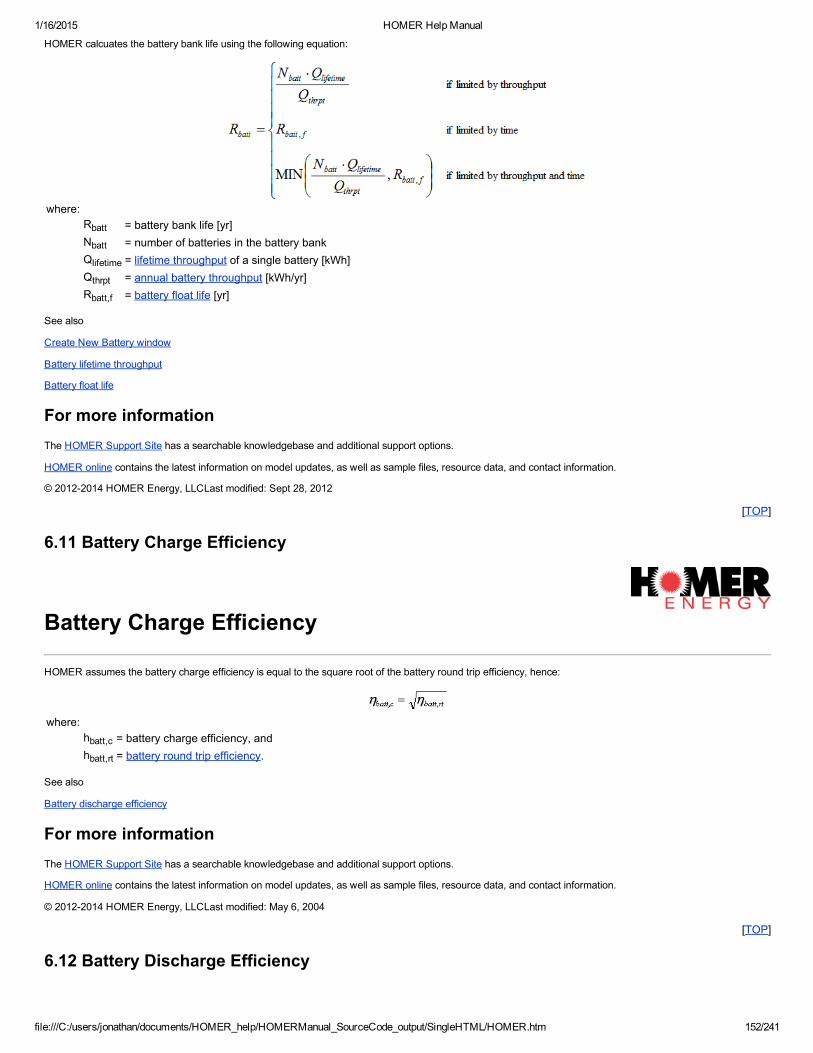
1/16/2015 HOMER Help Manual
file:///C:/users/jonathan/documents/HOMER_help/HOMERManual_SourceCode_output/SingleHTML/HOMER.htm 152/241
HOMER calcuates the battery bank life using the following equation:
where:Rbatt = battery bank life [yr]Nbatt = number of batteries in the battery bankQlifetime = lifetime throughput of a single battery [kWh]Qthrpt = annual battery throughput [kWh/yr]Rbatt,f = battery float life [yr]
See also
Create New Battery window
Battery lifetime throughput
Battery float life
For more informationThe HOMER Support Site has a searchable knowledgebase and additional support options.
HOMER online contains the latest information on model updates, as well as sample files, resource data, and contact information.
© 20122014 HOMER Energy, LLCLast modified: Sept 28, 2012
[TOP]
6.11 Battery Charge Efficiency
Battery Charge Efficiency
HOMER assumes the battery charge efficiency is equal to the square root of the battery round trip efficiency, hence:
where:hbatt,c = battery charge efficiency, andhbatt,rt = battery round trip efficiency.
See also
Battery discharge efficiency
For more informationThe HOMER Support Site has a searchable knowledgebase and additional support options.
HOMER online contains the latest information on model updates, as well as sample files, resource data, and contact information.
© 20122014 HOMER Energy, LLCLast modified: May 6, 2004
[TOP]
6.12 Battery Discharge Efficiency

1/16/2015 HOMER Help Manual
file:///C:/users/jonathan/documents/HOMER_help/HOMERManual_SourceCode_output/SingleHTML/HOMER.htm 153/241
Battery Discharge Efficiency
HOMER assumes the battery discharge efficiency is equal to the square root of the battery round trip efficiency, hence:
where:hbatt,d = battery discharge efficiency, andhbatt,rt = battery round trip efficiency.
See also
Battery charge efficiency
For more informationThe HOMER Support Site has a searchable knowledgebase and additional support options.
HOMER online contains the latest information on model updates, as well as sample files, resource data, and contact information.
© 20122014 HOMER Energy, LLCLast modified: May 6, 2004
[TOP]
6.13 Battery Energy Cost
Battery Energy Cost
Type: Intermediate VariableUnits: $/kWhSymbol: cbe,n
In any time step, the battery energy cost is the average cost of the energy that the system has put into the battery bank up until that time step. HOMER uses thefollowing equation to calculate the battery energy cost in each time step:
[$]where:
cbe,n = the battery energy cost in time step n [$/kWh]Ccc,i = the cost of cycle charging the battery in time step iEbc,i = the amount of energy that went into the battery bank in time step i [kWh]
The battery energy cost reflects the average cost that the system has incurred for deliberately charging the battery bank. The "cost of cycle charging," whichappears in the numerator of the above equation, is the extra cost incurred by the system specifically for charging the battery. Excess electricity that charges thebattery bank in some time step represents no such cost. But if the generator produced more power than required to serve the load, and it did so specifically tocharge the battery, then that act of charging the battery bank does cause the system to incur extra cost. The same is true if the system purchases extra grid powerexpressly to charge the battery. Such events occur routinely under the cycle charging strategy.
In any time step in which a generator or the grid cycle charges the battery, HOMER calculates the cycle charge cost by taking the actual cost of operating thesystem in that time step and subtracting the cost that would have occurred in that time step had the system not charged the battery.
The battery energy cost will always be zero under the load following dispatch strategy, because under load following the system never pays to charge the batterybank, it only uses excess electricity to charge the battery bank.
The battery bank's marginal cost of generation is equal to the sum of the battery wear cost and the battery energy cost.
See also
Battery wear cost
Cycle charging strategy
Load following strategy

1/16/2015 HOMER Help Manual
file:///C:/users/jonathan/documents/HOMER_help/HOMERManual_SourceCode_output/SingleHTML/HOMER.htm 154/241
For more informationThe HOMER Support Site has a searchable knowledgebase and additional support options.
HOMER online contains the latest information on model updates, as well as sample files, resource data, and contact information.
© 20122014 HOMER Energy, LLCLast modified: June 3, 2010
[TOP]
6.14 Battery Float Life
Battery Float Life
Type: Input VariableUnits: yrSymbol: Rbatt,f
The float life of the battery is the length of time that the battery will last before it needs replacement. When you create a battery you can choose whether to limit itslife by time, by throughput, or by both. The float life does not apply if you have chosen to limit the battery lifetime by throughput only.
HOMER uses the float life to calculate the battery bank life.
See also
Battery lifetime throughput
Battery bank life
For more informationThe HOMER Support Site has a searchable knowledgebase and additional support options.
HOMER online contains the latest information on model updates, as well as sample files, resource data, and contact information.
© 20122014 HOMER Energy, LLCLast modified: Sept 28, 2012
[TOP]
6.15 Battery Maximum Charge Rate
Battery Maximum Charge Rate
Type: Input VariableUnits: A/Ah of unfilled capacitySymbol: ac
The maximum charge rate variable imposes a limit on the rate at which the system can charge the battery bank. That limit is directly proportional to the amount of"unfilled capacity" in the battery, where the unfilled capacity is defined as the battery's maximum capacity minus its current absolute state of charge.
For example, consider a battery whose maximum capacity is 350 Ah and whose maximum charge rate is 0.4 A/Ah. If at some point in time the battery's absolutestate of charge is 310 Ah, then it has 40 Ah of unfilled capacity, so the highest charge current it could accept would be 40 Ah * 0.4 A/Ah = 16 A. If at some otherpoint in time its state of charge was 335 Ah, then the highest charge current it could accept would be only 6 A. So the allowable charge current decreases withincreasing state of charge.
Another variable, the maximum charge current, imposes an upper limit on the allowable charge current, regardless of the state of charge. If our example batterywere empty, the maximum charge rate variable would imply that it could accept a charge current of as high as 350 Ah * 0.4 A/Ah = 140 A. But a current that highmight be very damaging to the battery. If you set the maximum charge current variable to 25 A, then HOMER ensures that the charge current never exceeds 25 A,no matter what the state of charge.
Notes:
1. The kinetic battery model imposes a separate limit on the rate of charge.2. This discussion relates to a single battery. To find the maximum battery charge power, HOMER calculates the product of the maximum charge current times
the nominal voltage times the number of batteries in the battery bank.

1/16/2015 HOMER Help Manual
file:///C:/users/jonathan/documents/HOMER_help/HOMERManual_SourceCode_output/SingleHTML/HOMER.htm 155/241
For more informationThe HOMER Support Site has a searchable knowledgebase and additional support options.
HOMER online contains the latest information on model updates, as well as sample files, resource data, and contact information.
© 20122014 HOMER Energy, LLCLast modified: Sept 28, 2012
[TOP]
6.16 Battery Minimum State Of Charge
Battery Minimum State Of Charge
Type: Input VariableUnits: %Symbol: qmin
The relative state of charge below which the battery bank is never drawn specified as a percentage of the total capacity. Most rechargeable batteries are notmeant to be fully discharged. In fact, fully discharging some batteries can permanently damage them. The minimum state of charge is typically set to 3050% inorder to avoid damaging the battery bank by excessive discharge.
For more informationThe HOMER Support Site has a searchable knowledgebase and additional support options.
HOMER online contains the latest information on model updates, as well as sample files, resource data, and contact information.
© 20122014 HOMER Energy, LLCLast modified: Sept 28, 2012
[TOP]
6.17 Battery Roundtrip Efficiency
Battery Roundtrip Efficiency
Type: Input VariableUnits: %Symbol: hbatt,rt
The round trip DCtostoragetoDC energetic efficiency of the battery bank, or the fraction of energy put into the battery that can be retrieved. Typically this isabout 80%. HOMER assumes the battery charge efficiency and the battery discharge efficiency are both equal to the square root of the roundtrip efficiency.
See also
Battery charge efficiency
Battery discharge efficiency
For more informationThe HOMER Support Site has a searchable knowledgebase and additional support options.
HOMER online contains the latest information on model updates, as well as sample files, resource data, and contact information.
© 20122014 HOMER Energy, LLCLast modified: Sept 28, 2012
[TOP]
6.18 Battery Throughput

1/16/2015 HOMER Help Manual
file:///C:/users/jonathan/documents/HOMER_help/HOMERManual_SourceCode_output/SingleHTML/HOMER.htm 156/241
Battery Throughput
Type: Output VariableUnits: kWh/yrSymbol: Qthrpt
The battery throughput is the amount of energy that cycles through the battery bank in one year. Throughput is defined as the change in energy level of the batterybank, measured after charging losses and before discharging losses. This value is used to calculate the life of the battery bank.
For more informationThe HOMER Support Site has a searchable knowledgebase and additional support options.
HOMER online contains the latest information on model updates, as well as sample files, resource data, and contact information.
© 20122014 HOMER Energy, LLCLast modified: Sept 28, 2012
[TOP]
6.19 Battery Wear Cost
Battery Wear Cost
Type: Intermediate VariableUnits: $/kWhSymbol: cbw
The battery wear cost is the cost of cycling energy through the battery bank. If the battery properties indicate that the battery life is limited by throughput, thenHOMER assumes the battery bank will require replacement once its total throughput equals its lifetime throughput. Each kWh of throughput therefore brings thebattery bank that much closer to needing replacement. HOMER calculates the battery wear cost using the following equation:
where:Crep,batt = replacement cost of the battery bank [$]Nbatt = the number of batteries in the battery bankQlifetime = the lifetime throughput of a single battery [kWh]hrt = battery roundtrip efficiency [fractional]
The battery bank's marginal cost of generation is equal to the sum of the battery wear cost and the battery energy cost.
See also
Battery energy cost
Cycle charging strategy
Load following strategy
For more informationThe HOMER Support Site has a searchable knowledgebase and additional support options.
HOMER online contains the latest information on model updates, as well as sample files, resource data, and contact information.
© 20122014 HOMER Energy, LLCLast modified: June 3, 2010
[TOP]
6.20 Biogas (PRO)

1/16/2015 HOMER Help Manual
file:///C:/users/jonathan/documents/HOMER_help/HOMERManual_SourceCode_output/SingleHTML/HOMER.htm 157/241
Biogas
In HOMER, the term biogas refers to gasified biomass. Biomass feedstock (such as wood waste, agricultural residue, or energy crops) can be gasified by thermochemical or biological processes, and the product may be called one of several different names, including synthesis gas, syngas, producer gas, and wood gas.
Whatever the feedstock and the means of gasification, the major constituent gases of biogas are typically carbon monoxide, hydrogen, and carbon dioxide, plus asignificant amount of nitrogen (about 50% by weight) if thermal gasification is performed in the presence of air. Minor constituent gases include methane and watervapor.
Biogas typically has a low heating value compared with fossil fuels, particularly if it contains a large amount of nitrogen, which is noncombustible. But it has severaladvantages over solid biomass, including cleaner combustion, higher efficiency, and better control.
For more informationThe HOMER Support Site has a searchable knowledgebase and additional support options.
HOMER online contains the latest information on model updates, as well as sample files, resource data, and contact information.
© 20122014 HOMER Energy, LLCLast modified: May 6, 2004
[TOP]
6.21 Biomass Carbon Content (PRO)
Biomass Carbon Content
Type: Input Variable
Units: %Symbol: kbio
The amount of carbon contained in the biomass feedstock, expressed as a massbased percentage. HOMER uses this value to calculate the emissions of CO2,CO, and unburned hydrocarbons.
Tip: if you want HOMER to calculate the system's gross carbon emissions, then you should enter the gross carbon content of the biomass feedstock, which istypically on the order of 50%. On the other hand, if you want HOMER to calculate the system's net carbon emissions, then you should enter the net carbon contentof the feedstock, which is typically near zero. The net value takes into account the fact that the carbon in the biomass feedstock was originally absorbed from theatmosphere, and consuming that feedstock as fuel simply puts that carbon back into the atmosphere. The net effect on the atmosphere is near zero if the feedstockis harvested in a sustainable manner, meaning that the rate of consumption of biomass feedstock does not exceed the biosphere's ability to regenerate thatfeedstock.
A precise estimate of the net carbon content of a biomass feedstock will take into account the carbon emissions associated with the harvesting and processing ofthe feedstock. It may also account for avoided methane emissions related to the natural decomposition of the feedstock that would have occurred were it not for theconsumption of that feedstock to produce energy.
See also:
How HOMER calculates emissions
For more informationThe HOMER Support Site has a searchable knowledgebase and additional support options.
HOMER online contains the latest information on model updates, as well as sample files, resource data, and contact information.
2012 HOMER Energy, LLCLast modified:
[TOP]
6.22 Biomass Gasification Ratio (PRO)
Biomass Gasification Ratio

1/16/2015 HOMER Help Manual
file:///C:/users/jonathan/documents/HOMER_help/HOMERManual_SourceCode_output/SingleHTML/HOMER.htm 158/241
Type: Input VariableUnits: kg gas / kg biomassSymbol: fgas
The ratio of biogas generated to biomass feedstock consumed in the gasifier. HOMER assumes this value is constant.
For more information, see the article Operation of a Cofired Generator.
For more informationThe HOMER Support Site has a searchable knowledgebase and additional support options.
HOMER online contains the latest information on model updates, as well as sample files, resource data, and contact information.
© 20122014 HOMER Energy, LLCLast modified: Sept 28, 2012
[TOP]
6.23 Biomass Resource Cost (PRO)
Biomass Resource Cost
Type: Input VariableUnits: $/tSymbol: cbio
The cost per tonne (1000 kg) of biomass feedstock.
For more informationThe HOMER Support Site has a searchable knowledgebase and additional support options.
HOMER online contains the latest information on model updates, as well as sample files, resource data, and contact information.
© 2012 HOMER Energy, LLCLast modified: Sept 28, 2012
[TOP]
6.24 Biomass Substitution Ratio (PRO)
Biomass Substitution Ratio
Type: Input VariableUnits: noneSymbol: zgas
The ratio with which the biogas replaces fossil fuel in a cofired generator. If 8 kg/hr of biogas is required to replace 1 kg/hr of fossil fuel to maintain output power,the substitution ratio is 8. This ratio is assumed to be constant, independent of fuel mixture or output power.
If the fossil fuel burned by the generator is gaseous, the substitution ratio will be roughly equal to the ratio of the lower heating values of the fossil fuel and biogas.For example, if the cofired generator runs on a mixture of propane and biogas and the LHV of the biogas is onethird that of propane, the substitution ratio will likelybe approximately 3.
For liquid fossil fuels, the substitution ratio is typically somewhat higher than the LHV ratio because the generator does not operate as efficiently on the mixture ofbiogas and liquid fuel as it would on liquid fuel alone.
For more information, see the article Operation of a Cofired Generator.
For more informationThe HOMER Support Site has a searchable knowledgebase and additional support options.

1/16/2015 HOMER Help Manual
file:///C:/users/jonathan/documents/HOMER_help/HOMERManual_SourceCode_output/SingleHTML/HOMER.htm 159/241
HOMER online contains the latest information on model updates, as well as sample files, resource data, and contact information.
© 20122014 HOMER Energy, LLCLast modified: Sept 28, 2012
[TOP]
6.25 Boiler Marginal Cost (PRO)
Boiler Marginal Cost
Type: Intermediate VariableUnits: $/kWhSymbol: cboiler
The marginal cost of thermal energy from the boiler. HOMER uses this value when calculating the levelized cost of energy. HOMER calculates the boiler marginalcost with the following equation:
where:cfuel = cost of fuel [$/kg of fuel]cboiler,emissions = cost penalty associated with emissions from the boiler [$/kg of fuel]hboiler = boiler efficiency [unitless]LHVfuel = the lower heating value of the boiler fuel [MJ/kg]
The factor of 3.6 in the above equation arises because 1 kWh = 3.6 MJ.
Note: The fuel cost in the above equation is per kg, not per L or m3. For fuels denominated in volumetric units, HOMER calculates the cost per kg using the fueldensity.
HOMER calculates the cost penalty associated with boiler emissions using the following equation:
where:cCO2 = penalty for emissions of CO2 [$/t]cCO = penalty for emissions of CO [$/t]cUHC = penalty for emissions of unburned hydrocarbons (UHC) [$/t]cPM = penalty for emissions of particulate matter (PM) [$/t]cSO2 = penalty for emissions of SO2 [$/t]cNOx = penalty for emissions of NOx [$/t]gCO2 = boiler's carbon dioxide emissions coefficient [kg CO2 / kg fuel]gCO = boiler's carbon monoxide emissions coefficient [kg CO / kg fuel]gUHC = boiler's unburned hydrocarbons emissions coefficient [kg UHC / kg fuel]gPM = boiler's particulate matter emissions coefficient [kg PM / kg fuel]gSO2 = boiler's SO2 emissions coefficient [kg SO2 / kg fuel]gNOx = boiler's NOx emissions coefficient [kg NOx / kg fuel]
HOMER calculates the CO2 emissions coefficient using the following equation:
where:fC,fuel = the carbon content of the fuel [unitless]gCO = boiler's carbon monoxide emissions coefficient [kg CO / kg fuel]
gUHC = boiler's unburned hydrocarbons emissions coefficient [kg UHC / kg fuel]

1/16/2015 HOMER Help Manual
file:///C:/users/jonathan/documents/HOMER_help/HOMERManual_SourceCode_output/SingleHTML/HOMER.htm 160/241
Note that the factors of 44/12 and 12/28 in the above equation arise because the molecular weights of C, CO, and CO2 are equal to 12, 28, and 44 respectively.
HOMER calculates the SO2 emissions coefficient using the following equation:
where:fS,fuel = the sulfur content of the fuel [unitless]gUHC = boiler's unburned hydrocarbons emissions coefficient [kg UHC / kg fuel]xPM = the proportion of fuel sulfur converted to particulate matter [unitless]
Note that the factor of 2 in the above equation arises because the molecular weight of SO2 (64) is twice that of S (32).
See also:
Levelized cost of energy
For more informationThe HOMER Support Site has a searchable knowledgebase and additional support options.
HOMER online contains the latest information on model updates, as well as sample files, resource data, and contact information.
© 20122014 HOMER Energy, LLCLast modified: May 12, 2005
[TOP]
6.26 Breakeven Grid Extension Distance (PRO)
Breakeven Grid Extension Distance
Type: Output VariableUnits: kmSymbol: Dgrid
The distance from the grid which makes the net present cost of extending the grid equal to the net present cost of the standalone system. Farther away from thegrid, the standalone system is optimal. Nearer to the grid, grid extension is optimal.
HOMER calculates the breakeven grid extension distance using the following equation:
where:CNPC = total net present cost of the standalone power system [$]CRF() = capital recovery factori = interest rate [%]Rproj = project lifetime [yr]Edemand = total annual electrical demand (primary plus deferrable) [kWh/yr]cpower = cost of power from the grid [$/kWh]ccap = capital cost of grid extension [$/km]com = O&M cost of grid extension [$/yr/km]
For more informationThe HOMER Support Site has a searchable knowledgebase and additional support options.
HOMER online contains the latest information on model updates, as well as sample files, resource data, and contact information.
© 20122014 HOMER Energy, LLCLast modified: Sept 28, 2012
[TOP]
6.27 Capacity Shortage

1/16/2015 HOMER Help Manual
file:///C:/users/jonathan/documents/HOMER_help/HOMERManual_SourceCode_output/SingleHTML/HOMER.htm 161/241
Capacity Shortage
An capacity shortage is a shortfall that occurs between the required operating capacity and the actual amount of operating capacity the system can provide.HOMER keeps track of such shortages and calculates the total amount that occurs over the year.
For example, consider a simple system consisting of a 50 kW AC generator serving an AC load:
If the load is 30 kW and the required operating reserve is 15 kW, the required operating capacity is 45 kW and the actual operating capacity is 50 kW, sothere is no capacity shortage. The generator would operate at 30 kW to meet the load, and the 20 kW of operating reserve it provides would satisfy therequirement.If the load is 40 kW and the required operating reserve is 12 kW, the required operating capacity is 52 kW and the actual operating capacity is 50 kW, so thecapacity shortage is 2 kW. The generator provides only 10 kW of operating reserve in this situation, not enough to satisfy the requirement.If the load is 55 kW and the required operating reserve is 0 kW, the required operating capacity is 55 kW and the actual operating capacity is 50 kW, so thecapacity shortage is 5 kW (and the unmet load is also 5 kW).If the load is 55 kW and the required operating reserve is 20 kW, the required operating capacity is 75 kW and the actual operating capacity is 50 kW, so thecapacity shortage is 25 kW (and the unmet load is 5 kW).
See also:
Required operating reserve
Maximum annual capacity shortage
Total capacity shortage
Capacity shortage fraction
For more informationThe HOMER Support Site has a searchable knowledgebase and additional support options.
HOMER online contains the latest information on model updates, as well as sample files, resource data, and contact information.
© 20122014 HOMER Energy, LLCLast modified: May 6, 2004
[TOP]
6.28 Capacity Shortage Fraction
Capacity Shortage Fraction
Type: Output VariableUnits: noneSymbol: fcs
The capacity shortage fraction is equal to the total capacity shortage divided by the total electrical demand. HOMER considers a system feasible (or acceptable)only if the capacity shortage fraction is less than or equal to the maximum annual capacity shortage. HOMER uses the following equation to calculate the capacityshortage fraction:
where:Ecs = total capacity shortage [kWh/yr]Edemand = total electrical demand (primary and deferrable load) [kWh/yr]
For more informationThe HOMER Support Site has a searchable knowledgebase and additional support options.
HOMER online contains the latest information on model updates, as well as sample files, resource data, and contact information.
© 20122014 HOMER Energy, LLCLast modified: Sept 28, 2012
[TOP]

1/16/2015 HOMER Help Manual
file:///C:/users/jonathan/documents/HOMER_help/HOMERManual_SourceCode_output/SingleHTML/HOMER.htm 162/241
6.29 Capacity Shortage Penalty
Capacity Shortage Penalty
Type: Input VariableUnits: $/kWhSymbol: ccs
The capacity shortage penalty is a cost penalty that HOMER applies to the system for any capacity shortage that occurs during the year. HOMER uses this value tocalculate the other O&M cost.
For more informationThe HOMER Support Site has a searchable knowledgebase and additional support options.
HOMER online contains the latest information on model updates, as well as sample files, resource data, and contact information.
© 20122014 HOMER Energy, LLCLast modified: Sept 28, 2012
[TOP]
6.30 Capital Recovery Factor
Capital Recovery Factor
The capital recovery factor is a ratio used to calculate the present value of an annuity (a series of equal annual cash flows). The equation for the capital recoveryfactor is:
where:i = real interest rateN = number of years
Example: for i = 7% and N = 5 years, the capital recovery factor is equal to 0.2439. A $1000 loan at 7% interest could therefore be paid back with 5 annualpayments of $243.90. The present value of the five annual payments of $243.90 is $1000.
See also
Sinking fund factor
For more informationThe HOMER Support Site has a searchable knowledgebase and additional support options.
HOMER online contains the latest information on model updates, as well as sample files, resource data, and contact information.
© 20122014 HOMER Energy, LLCLast modified: May 6, 2004
[TOP]
6.31 How HOMER Calculates the PV Cell Temperature
How HOMER Calculates the PV Cell Temperature
The PV cell temperature is the temperature of the surface of the PV array. During the night it is the same as the ambient temperature, but in full sun the cell

1/16/2015 HOMER Help Manual
file:///C:/users/jonathan/documents/HOMER_help/HOMERManual_SourceCode_output/SingleHTML/HOMER.htm 163/241
temperature can exceed the ambient temperature by 30°C or more.
If in the PV Array inputs window you choose to consider the effect of temperature on the PV array, then HOMER will calculate the cell temperature in each timestep, and use that in calculating the power output of the PV array. This article describes how HOMER calculates the cell temperature from the ambient temperatureand the radiation striking the array.
We start by defining an energy balance for the PV array, using the following equation from Duffie and Beckman (1991):
where:τ is the solar transmittance of any cover over the PV array [%]α is the solar absorptance of the PV array [%]GT is the solar radiation striking the PV array [kW/m2]ηc is the electrical conversion efficiency of the PV array [%]UL is the coefficient of heat transfer to the surroundings [kW/m2°C]Tc is the PV cell temperature [°C]Ta is the ambient temperature [°C]
The above equation states that a balance exists between, on one hand, the solar energy absorbed by the PV array, and on the other hand, the electrical outputplus the heat transfer to the surroundings. We can solve that equation for cell temperature to yield:
It is difficult to measure the value of (τα / UL) directly, so instead manufacturers report the nominal operating cell temperature (NOCT), which is defined as the celltemperature that results at an incident radiation of 0.8 kW/m2, an ambient temperature of 20°C, and no load operation (meaning ηc = 0). We can subsitute thesevalues into the above equation and solve it for τα/UL to yield the following equation:
where:Tc,NOCT is the nominal operating cell temperature [°C]Ta,NOCT is the ambient temperature at which the NOCT is defined [20°C]GT,NOCT is the solar radiation at which the NOCT is defined [0.8 kW/m2]
If we assume that τα/UL is constant, we can subsitute this equation into the cell temperature equation to yield:
HOMER assumes a value of 0.9 for τα in the above equation, as Duffie and Beckman (1991) suggest. Since the term ηc /τα is small compared to unity, thisassumption does not introduce significant error.
HOMER assumes that the PV array always operates at its maximum power point, as it would if it were controlled by a maximum power point tracker. That meansHOMER assumes the cell efficiency is always equal to the maximum power point efficiency:
where:ηmp is the efficiency of the PV array at its maximum power point [%]
So in the equation for cell temperature we can replace ηc with _mp to yield:
But ηmp depends on the cell temperature Tc. HOMER assumes that the efficiency varies linearly with temperature according to the following equation:
where:ηmp,STC is the maximum power point efficiency under standard test conditions [%]αP is the temperature coefficient of power [%/°C]Tc,STC is the cell temperature under standard test conditions [25°C]

1/16/2015 HOMER Help Manual
file:///C:/users/jonathan/documents/HOMER_help/HOMERManual_SourceCode_output/SingleHTML/HOMER.htm 164/241
The temperature coefficient of power is normally negative, meaning that the efficiency of the PV array decreases with increasing cell temperature.
We can substitute this efficiency equation into the preceding cell temperature equation and solve for cell temperature to yield:
The temperatures in the above equation must be in Kelvin. HOMER uses this equation to calculate the cell temperature in each time step.
See also
PV Inputs window
Standard test conditions
Nominal operating cell temperature
How HOMER calculates the radiation incident on the PV array
How HOMER calculates the PV array power output
Can HOMER model a maximum power point tracker?
For more informationThe HOMER Support Site has a searchable knowledgebase and additional support options.
HOMER online contains the latest information on model updates, as well as sample files, resource data, and contact information.
© 20122014 HOMER Energy, LLCLast modified: November 21, 2007
[TOP]
6.32 Clearness Index
Clearness Index
The clearness index is a measure of the clearness of the atmosphere. It is the fraction of the solar radiation that is transmitted through the atmosphere to strike thesurface of the Earth. It is a dimensionless number between 0 and 1, defined as the surface radiation divided by the extraterrestrial radiation. The clearness indexhas a high value under clear, sunny conditions, and a low value under cloudy conditions.
The clearness index can be defined on an instantaneous, hourly, or monthly basis. The clearness index values in HOMER's Solar Resource Inputs window aremonthly average values. The symbol for the monthly average clearness index is Kt.
Typical values of Kt range from 0.25 (a very cloudy month, such as an average December in London) to 0.75 (a very sunny month, such as an average June inPhoenix).
The table of solar data contains monthly average clearness indices for numerous locations around the world.
See also
How HOMER calculates clearness index
For more informationThe HOMER Support Site has a searchable knowledgebase and additional support options.
HOMER online contains the latest information on model updates, as well as sample files, resource data, and contact information.
© 20122014 HOMER Energy, LLCLast modified: July 16, 2004
[TOP]
6.33 CO Emissions Penalty (PRO)

1/16/2015 HOMER Help Manual
file:///C:/users/jonathan/documents/HOMER_help/HOMERManual_SourceCode_output/SingleHTML/HOMER.htm 165/241
CO Emissions Penalty
Type: Input VariableUnits: $/tSymbol: cCO
Use the CO emissions penalty to penalize systems for their production of carbon monoxide. HOMER uses this input value when calculating the Other O&M cost.
For more informationThe HOMER Support Site has a searchable knowledgebase and additional support options.
HOMER online contains the latest information on model updates, as well as sample files, resource data, and contact information.
© 20122014 HOMER Energy, LLCLast modified: Sept 28, 2012
[TOP]
6.34 CO2 Emissions Penalty
CO2 Emissions Penalty
Type: Input VariableUnits: $/tSymbol: cCO2
Use the CO2 emissions penalty to penalize systems for their production of carbon dioxide. HOMER uses this input value when calculating the Other O&M cost.
For more informationThe HOMER Support Site has a searchable knowledgebase and additional support options.
HOMER online contains the latest information on model updates, as well as sample files, resource data, and contact information.
© 20122014 HOMER Energy, LLCLast modified: Sept 28, 2012
[TOP]
6.35 Component
Component
In HOMER, the term "component" refers to any part of the system that generates, stores or transfers electric or thermal energy, and whose size or quantity is anoptimization variable.
Photovoltaic panels, diesel generators and wind turbines are examples of components. Less obvious are things like converters, electrolyzers and the utility grid.
For more informationThe HOMER Support Site has a searchable knowledgebase and additional support options.
HOMER online contains the latest information on model updates, as well as sample files, resource data, and contact information.
© 20122014 HOMER Energy, LLCLast modified: May 6, 2004
[TOP]
6.36 Component Library

1/16/2015 HOMER Help Manual
file:///C:/users/jonathan/documents/HOMER_help/HOMERManual_SourceCode_output/SingleHTML/HOMER.htm 166/241
Component Library
The component library is a collection of properties of batteries, flywheels, wind turbines, and fuels. Wherever you need to select a type of battery, flywheel, windturbine, or fuel, HOMER uses the component library to generate a list of available types. In the example shown below, taken from the Wind Turbine Inputs window,HOMER is displaying a list of the wind turbine types contained in the component library.
You can add and remove items from the component library using the New and Delete buttons on the battery, flywheel, wind turbine, generator, and boilerwindows.
Note that the component library contains performance data, but no cost data.
For more informationThe HOMER Support Site has a searchable knowledgebase and additional support options.
HOMER online contains the latest information on model updates, as well as sample files, resource data, and contact information.
© 20122014 HOMER Energy, LLCLast modified: October 21, 2009
[TOP]
6.37 Cycle Charging Strategy
Cycle Charging Strategy
The cycle charging strategy is a dispatch strategy whereby whenever a generator needs to operate to serve the primary load, it operates at full output power.Surplus electrical production goes toward the lowerpriority objectives such as, in order of decreasing priority: serving the deferrable load, charging the batterybank, and serving the electrolyzer.
Note: A generator will not produce surplus power just to dump it as excess electricity. There must be some use for its surplus power for HOMER to operate itabove the level needed to serve the primary load.
When using the cycle charging strategy, HOMER dispatches the controllable power sources (generators, battery bank, grid) each time step of the simulation in atwostep process. First, HOMER selects the optimal combination of power sources to serve the primary and thermal load according to the loadfollowing strategy.Then HOMER ramps up the output of each generator in that optimal combination to its rated capacity, or as close as possible without causing excess electricity.
If a setpoint state of charge is applied to the cycle charging strategy, then when the battery state of charge is below the setpoint and the battery was notdischarging in the previous time step, HOMER will avoid discharging the battery in this time step. A generator will likely be called upon to serve the primary loadand produce excess electricity to charge the battery bank. So once the system starts charging the battery bank it continues to do so until it reaches the setpointstate of charge.
See also
Load following strategy
Setpoint state of charge
1/16/2015 HOMER Help Manual
file:///C:/users/jonathan/documents/HOMER_help/HOMERManual_SourceCode_output/SingleHTML/HOMER.htm 167/241
For more informationThe HOMER Support Site has a searchable knowledgebase and additional support options.
HOMER online contains the latest information on model updates, as well as sample files, resource data, and contact information.
© 20122014 HOMER Energy, LLCLast modified: May 6, 2004
[TOP]
6.38 DC Primary Load Served
DC Primary Load Served
Type: Output VariableUnits: kWh/yrSymbol: Eprim, DC
The DC primary load served is the total amount of energy that went towards serving the DC primary load(s) during the year.
For more informationThe HOMER Support Site has a searchable knowledgebase and additional support options.
HOMER online contains the latest information on model updates, as well as sample files, resource data, and contact information.
© 20122014 HOMER Energy, LLCLast modified: Sept 28, 2012
[TOP]
6.39 Decision Variable
Decision Variable
A decision variable is a variable whose optimal value is determined during the course of the optimization process. An example is the size of the PV array. If you areusing SearchSizer , HOMER will automatically determine the optimal values for your PV array size. If you are specifying your own Search Space , HOMERconsiders each different PV array size you specify and finds the value that results in the least net present cost.
The decision variables in HOMER are:
the size of the PV arraythe number of wind turbinesthe size of the hydro systemthe size of each generatorthe number of batteriesthe size of the converterthe size of the electrolyzerthe size of the hydrogen storage tankthe dispatch strategythe maximum grid demand
Decision variables are also known as optimization variables.
For more informationThe HOMER Support Site has a searchable knowledgebase and additional support options.
HOMER online contains the latest information on model updates, as well as sample files, resource data, and contact information.
© 2012 HOMER Energy, LLCLast modified: May 6, 2004
[TOP]

1/16/2015 HOMER Help Manual
file:///C:/users/jonathan/documents/HOMER_help/HOMERManual_SourceCode_output/SingleHTML/HOMER.htm 168/241
6.40 Deferrable Load Served (PRO)
Deferrable Load Served
Type: Output VariableUnits: kWh/yrSymbol: Edef
The deferrable load served is the total amount of energy that went towards serving the deferrable load during the year.
For more informationThe HOMER Support Site has a searchable knowledgebase and additional support options.
HOMER online contains the latest information on model updates, as well as sample files, resource data, and contact information.
© 20122014 HOMER Energy, LLCLast modified: Sept 28, 2012
[TOP]
6.41 Deltaplot
Deltaplot
The deltaplot shows the frequency of changes in any variable over some length of time. Choose the variable from the dropdown box, and choose the length oftime using the slider control.
For more informationThe HOMER Support Site has a searchable knowledgebase and additional support options.
HOMER online contains the latest information on model updates, as well as sample files, resource data, and contact information.
© 2012 HOMER Energy, LLCLast modified: January 21, 2010
[TOP]
6.42 Design Flow Rate (PRO)
Design Flow Rate
Type: Input VariableUnits: L/sSymbol:
The design flow rate is the flow rate for which the hydro turbine is designed. This is also typically the flow rate at which the turbine operates at its maximumefficiency, although HOMER assumes the turbine efficiency is constant.
HOMER uses the design flow rate to calculate the hydro turbine flow rate and the nominal hydro power.
See also
Minimum flow rate

1/16/2015 HOMER Help Manual
file:///C:/users/jonathan/documents/HOMER_help/HOMERManual_SourceCode_output/SingleHTML/HOMER.htm 169/241
Maximum flow rate
For more informationThe HOMER Support Site has a searchable knowledgebase and additional support options.
HOMER online contains the latest information on model updates, as well as sample files, resource data, and contact information.
© 20122014 HOMER Energy, LLCLast modified: Sept 28, 2012
[TOP]
6.43 Discount Factor
Discount Factor
The discount factor is a ratio used to calculate the present value of a cash flow that occurs in any year of the project lifetime. HOMER calculates the discount factorusing the following equation:
where:i = real interest rate [%]N = number of years
Example: for i = 5% and N = 12 years, the discount factor equals 0.557. That means a $1000 nominal cash flow in year 12 has a present value of $557. In otherwords, a $1000 cash flow in year 12 is equivalent to a $557 cash flow in year zero. This is a demonstration of the time value of money: a dollar now is worth morethan a dollar twelve years in the future.
See also
Present value
For more informationThe HOMER Support Site has a searchable knowledgebase and additional support options.
HOMER online contains the latest information on model updates, as well as sample files, resource data, and contact information.
© 20122014 HOMER Energy, LLCLast modified: June 16, 2008
[TOP]
6.44 Dispatch Strategy
Dispatch Strategy
A dispatch strategy is a set of rules used to control the operation of the generator(s) and the battery bank whenever there is insufficient renewable energy to supplythe load. See Barley and Winn, 1996 for a complete discussion of hybrid system dispach strategies.
See also
System Control Inputs
For more informationThe HOMER Support Site has a searchable knowledgebase and additional support options.
HOMER online contains the latest information on model updates, as well as sample files, resource data, and contact information.
© 20122014 HOMER Energy, LLCLast modified: October 29, 2004
[TOP]

1/16/2015 HOMER Help Manual
file:///C:/users/jonathan/documents/HOMER_help/HOMERManual_SourceCode_output/SingleHTML/HOMER.htm 170/241
6.45 Diurnal Pattern Strength
Diurnal Pattern Strength
Type: Input VariableUnits: noneSymbol: dTypical Range: 0.0 0.4
The diurnal pattern strength is a number between 0 and 1 that reflects how strongly the wind speed tends to depend on the time of day. When you generatesynthetic wind speed data, HOMER assumes a cosinusoidal diurnal pattern, with the diurnal pattern strength defined as the ratio of the amplitude to the mean.
The following equation describes the average diurnal profile of the synthesized wind speed data:
where:Ui = the mean wind speed in hour i [m/s]U = the overall mean wind speed [m/s]d = diurnal pattern strength (a number between 0 and 1)f = hour of peak windspeed (an integer between 1 and 24)
Note that the character of the diurnal pattern tends to vary significantly with height above ground. The following graph shows a typical example, where at 10mabove ground the wind speed tends to peak in the afternoon, wherease at 60m above ground, the wind speed tends to peak overnight. This graph shows datameasured at a site in the Midwest region of the US:
This pattern can be very pronounced, such as in the following graph, which shows mean diurnal profiles at heights from 10m to 100m above ground, at a location inthe Great Plains region of the US. In this example, the diurnal pattern at 100m is almost the mirror image of that at 10m above ground:
In other cases, the diurnal pattern changes much less with height above ground, such as in the following graph:

1/16/2015 HOMER Help Manual
file:///C:/users/jonathan/documents/HOMER_help/HOMERManual_SourceCode_output/SingleHTML/HOMER.htm 171/241
Since HOMER will use the wind speeds to estimate wind turbine power output, you want the wind speed data to reflect, as closely as possible, the conditions at thehub height of the wind turbine. So consider the height above ground when you specify the diurnal pattern strength and the hour of peak wind speed.
To measure the diurnal pattern strength from time series wind speed data, one can calculate the average diurnal profile and perform a curve fit operation to find thebestfit value of the hour of peak wind speed and the diurnal pattern strength. We performed that process for the 239 weather stations in the U.S. National SolarRadiation Data Base, which record wind speeds at 10m above ground. The histogram below shows the distribution of the diurnal pattern strength values that wemeasured. The measured values themselves appear in the table of measured wind parameters.
For more informationThe HOMER Support Site has a searchable knowledgebase and additional support options.
HOMER online contains the latest information on model updates, as well as sample files, resource data, and contact information.
© 20122014 HOMER Energy, LLCLast modified: Sept 28, 2012
[TOP]
6.46 DMap
DMap
A DMap (data map) is a type of graph showing one year of time series data. With time of day on one axis and day of the year on the other, each time steps of theyear is represented by a rectangle which is colored according to the data value for that hour. The DMap format often allows you to see daily and seasonal patternsmore easily than you could with a simple time series plot. An example of a DMap appears below:
For more informationThe HOMER Support Site has a searchable knowledgebase and additional support options.

1/16/2015 HOMER Help Manual
file:///C:/users/jonathan/documents/HOMER_help/HOMERManual_SourceCode_output/SingleHTML/HOMER.htm 172/241
HOMER online contains the latest information on model updates, as well as sample files, resource data, and contact information.
© 20122014 HOMER Energy, LLCLast modified: May 6, 2004
[TOP]
6.47 Effective Head (PRO)
Effective Head
Type: Intermediate Variable
Units: mSymbol: hnet
One can model the friction pressure loss in the pipeline between the intake and the turbine as a loss in head. The effective head is the actual vertical drop minusthis head loss. HOMER calculates the effective head (or net head) using the following equation:
where:h = available head [m]fh = pipe head loss [%]
HOMER uses the effective head to calculate the power output of the hydro turbine in each time step.
See also
Available head
Calculating hydro power output
For more informationThe HOMER Support Site has a searchable knowledgebase and additional support options.
HOMER online contains the latest information on model updates, as well as sample files, resource data, and contact information.
© 20122014 HOMER Energy, LLCLast modified: December 27, 2007
[TOP]
6.48 Electrolyzer Efficiency (PRO)
Electrolyzer Efficiency
Type: Input VariableUnits: %Symbol: helectrolyzer
The efficiency with which the electrolyzer converts electricity into hydrogen. This is equal to the energy content (based on higher heating value) of the hydrogenproduced divided by the amount of electricity consumed.
Example: The higher heating value of hydrogen is 142 MJ/kg, which is equal to 39.4 kWh/kg. So an electrolyzer that consumes 50 kWh of electricity to produceone kilogram of hydrogen has an efficiency of 39.4 kWh/kg divided by 50 kWh/kg, which is 79%.
For more informationThe HOMER Support Site has a searchable knowledgebase and additional support options.
HOMER online contains the latest information on model updates, as well as sample files, resource data, and contact information.

1/16/2015 HOMER Help Manual
file:///C:/users/jonathan/documents/HOMER_help/HOMERManual_SourceCode_output/SingleHTML/HOMER.htm 173/241
© 20122014 HOMER Energy, LLCLast modified: Sept 28, 2012
[TOP]
6.49 Excess Electricity
Excess Electricity
Excess electricity is surplus electrical energy that must be dumped (or curtailed) because it cannot be used to serve a load or charge the batteries. Excesselectricity occurs when there is a surplus of power being produced (either by a renewable source or by the generator when its minimum output exceeds the load)and the batteries are unable to absorb it all.
A resistive heater (often called an electric boiler) can convert excess electricity into thermal energy that can meet the thermal load. You can model such a situationby going to the System Control Inputs window and checking the checkbox labeled Allow excess electricity to serve thermal load.
If it cannot be put to use, excess electricity may need to be dissipated in a dump load, which is usually a simple resistive heater or a bank of light bulbs. In somecases, excess energy represents energy that could be curtailed rather than disappated.
HOMER tabulates the excess electricity experienced by the system in each time step. You can see the time series and the annual total in the Simulation Resultswindow, which appears when you double click on a system in the Optimization Results tab of HOMER's main window.
For more informationThe HOMER Support Site has a searchable knowledgebase and additional support options.
HOMER online contains the latest information on model updates, as well as sample files, resource data, and contact information.
© 20122014 HOMER Energy, LLCLast modified: May 6, 2004
[TOP]
6.50 Excess Electricity Fraction
Excess Electricity Fraction
Type: Output VariableUnits: noneSymbol: fexcess
The excess electricity fraction is the ratio of total excess electricity to the total electrical production. HOMER calculates this value at the end of each simulation usingthe following equation:
where:Eexcess = total excess electricity [kWh/yr]Eprod = total electrical production [kWh/yr]
See also
Total excess energy
For more informationThe HOMER Support Site has a searchable knowledgebase and additional support options.
HOMER online contains the latest information on model updates, as well as sample files, resource data, and contact information.
© 20122014 HOMER Energy, LLCLast modified: Sept 28, 2012
[TOP]

1/16/2015 HOMER Help Manual
file:///C:/users/jonathan/documents/HOMER_help/HOMERManual_SourceCode_output/SingleHTML/HOMER.htm 174/241
6.51 Feasible and Infeasible Systems
Feasible and Infeasible Systems
A feasible system is one that satisfies the constraints. An infeasible system is one that does not satisfy the constraints.
HOMER discards infeasible systems and does not display them in the optimization results or sensitivity results.
See also:
The definition of a system
Optimization results
Sensitivity results
Constraints
For more informationThe HOMER Support Site has a searchable knowledgebase and additional support options.
HOMER online contains the latest information on model updates, as well as sample files, resource data, and contact information.
© 20122014 HOMER Energy, LLCLast modified: October 29, 2004
[TOP]
6.52 Flow Rate Available To Hydro Turbine (PRO)
Flow Rate Available To Hydro Turbine
Type: Intermediate VariableUnits: m3/sSymbol:
The flow rate available to the hydro turbine is the maximum flow rate that could be diverted into the hydro turbine. In each time step, HOMER calculates theavailable flow rate using the following equation:
where:= the total stream flow [m3/s]= residual flow [m3/s]
HOMER uses the available stream flow to calculate the actual stream flow through the hydro turbine in each time step.
See also
Hydro turbine flow rate
Calculating the hydro power output
For more informationThe HOMER Support Site has a searchable knowledgebase and additional support options.
HOMER online contains the latest information on model updates, as well as sample files, resource data, and contact information.
© 2012 HOMER Energy, LLCLast modified: December 27, 2007
[TOP]
6.53 Fossil Fraction (PRO)

1/16/2015 HOMER Help Manual
file:///C:/users/jonathan/documents/HOMER_help/HOMERManual_SourceCode_output/SingleHTML/HOMER.htm 175/241
Fossil Fraction
A cofired generator can operate on a mixture of fossil fuel and biogas. The fossil fraction (xfossil) is the ratio of fossil fuel used by the generator in dualfuel mode tothat required to produce the same output power in pure fossil mode. With compressionignition (diesel) engines, it is necessary to maintain a minimum fossilfraction to ensure proper ignition.
For a more complete explanation of the fossil fraction and the operation of a cofired generator, please see the article Operation of a Cofired Generator.
See also
Minimum fossil fraction
Operation of a cofired generator
For more informationThe HOMER Support Site has a searchable knowledgebase and additional support options.
HOMER online contains the latest information on model updates, as well as sample files, resource data, and contact information.
© 20122014 HOMER Energy, LLCLast modified: May 6, 2004
[TOP]
6.54 Fuel Carbon Content
Fuel Carbon Content
Type: Input VariableUnits: % (by mass)Symbol: kfuel
The carbon content of the fuel as a percent of its mass. This value is used to calculate the annual emissions of carbon dioxide, carbon monoxide, and unburnedhydrocarbons resulting from the consumption of this fuel in a generator, boiler, or reformer.
See also:
How HOMER calculates emissions
CO2 emissions penalty
CO emissions penalty
Grid emissions factors
For more informationThe HOMER Support Site has a searchable knowledgebase and additional support options.
HOMER online contains the latest information on model updates, as well as sample files, resource data, and contact information.
© 20122014 HOMER Energy, LLCLast modified: Sept 28, 2012
[TOP]
6.55 Fuel Price
Fuel Price

1/16/2015 HOMER Help Manual
file:///C:/users/jonathan/documents/HOMER_help/HOMERManual_SourceCode_output/SingleHTML/HOMER.htm 176/241
Type: Input VariableUnits: $/LSymbol: cfuel
The price of fuel in dollars per liter. It is very common to do a sensitivity analysis on this variable for two reasons: it is difficult to accurately predict the future fuelprice, and the optimal architecture of the power system can vary widely depending on the fuel price.
This input is used to calculate the generator fuel cost.
For more informationThe HOMER Support Site has a searchable knowledgebase and additional support options.
HOMER online contains the latest information on model updates, as well as sample files, resource data, and contact information.
© 20122014 HOMER Energy, LLCLast modified: Sept 28, 2012
[TOP]
6.56 Fuel Sulfur Content
Fuel Sulfur Content
Type: Input VariableUnits: % (by mass)
The sulfur content of the fuel as a percent of its mass. This value is used to calculate the annual emissions of particulate matter and sulfur dioxide resulting from theconsumption of this fuel in a generator, boiler, or reformer.
See also:
How HOMER calculates emissions
SO2 emissions penalty
PM emissions penalty
Grid emissions factors
For more informationThe HOMER Support Site has a searchable knowledgebase and additional support options.
HOMER online contains the latest information on model updates, as well as sample files, resource data, and contact information.
© 20122014 HOMER Energy, LLCLast modified: Sept 28, 2012
[TOP]
6.57 Future Value
Future Value
The future value is defined as the equivalent value at some designated future date of a sequence of cash flows, taking into account the time value of money.
See also
Interest rate
Sinking fund factor
Present value
For more information

1/16/2015 HOMER Help Manual
file:///C:/users/jonathan/documents/HOMER_help/HOMERManual_SourceCode_output/SingleHTML/HOMER.htm 177/241
The HOMER Support Site has a searchable knowledgebase and additional support options.
HOMER online contains the latest information on model updates, as well as sample files, resource data, and contact information.
© 20122014 HOMER Energy, LLCLast modified: May 6, 2004
[TOP]
6.58 Generator
Generator
In HOMER, a "generator" is a device that consumes fuel to produce electric (and sometimes thermal) energy. Generators can be dispatched, meaning the systemcan turn them on as necessary. Microturbines and fuel cells are generators, as are diesel and gasolinefueled reciprocating engine generators.
For more informationThe HOMER Support Site has a searchable knowledgebase and additional support options.
HOMER online contains the latest information on model updates, as well as sample files, resource data, and contact information.
© 20122014 HOMER Energy, LLCLast modified: May 6, 2004
[TOP]
6.59 Generator Average Electrical Efficiency
Generator Average Electrical Efficiency
Type: Output VariableUnits: %Symbol: hgen
This is the average electrical efficiency of the generator over the year, defined as the electrical energy out divided by fuel energy in. HOMER uses the followingequation to calculate the average electrical efficiency:
where:Egen = the generator's total annual electrical production [kWh/yr]mfuel = the generator's total annual fuel consumption [kg/yr]LHVfuel = the lower heating value of the fuel [MJ/kg]
The factor of 3.6 in the above equation arises because 1 kWh = 3.6 MJ.
See also:
Generator average total efficiency
For more informationThe HOMER Support Site has a searchable knowledgebase and additional support options.
HOMER online contains the latest information on model updates, as well as sample files, resource data, and contact information.
© 20122014 HOMER Energy, LLCLast modified: Sept 28, 2012
[TOP]
6.60 Generator Average Total Efficiency

1/16/2015 HOMER Help Manual
file:///C:/users/jonathan/documents/HOMER_help/HOMERManual_SourceCode_output/SingleHTML/HOMER.htm 178/241
Generator Average Total Efficiency
Type: Output VariableUnits: %Symbol: hgen,tot
This is the average total efficiency of the generator over the year, defined as the electrical plus thermal energy out divided by fuel energy in. HOMER uses thefollowing equation to calculate the average total efficiency:
where:Egen = the generator's total annual electrical production [kWh/yr]
Egen = the generator's total annual thermal production [kWh/yr]mfuel = the generator's total annual fuel consumption [kg/yr]LHVfuel = the lower heating value of the fuel [MJ/kg]
The factor of 3.6 in the above equation arises because 1 kWh = 3.6 MJ.
See also:
Generator average efficiency
For more informationThe HOMER Support Site has a searchable knowledgebase and additional support options.
HOMER online contains the latest information on model updates, as well as sample files, resource data, and contact information.
© 20122014 HOMER Energy, LLCLast modified: Sept 28, 2012
[TOP]
6.61 Generator Carbon Monoxide Emissions Factor
Generator Carbon Monoxide Emissions Factor
Type: Input VariableUnits: grams per unit fuel (fuel units can be L, m3, or kg)Symbol: fgen,CO
The amount of carbon monoxide emitted per unit fuel consumed by the generator. Because carbon monoxide is a product of incomplete combustion, the quantityproduced will depend on the fuel, engine design, and operating conditions, including the power output of the generator. But HOMER makes a simplifyingassumption that this factor is constant.
The following graph shows the value of the carbon monoxide emissions factor for diesel generators in the size range 50 kW 450 kW. The source of these data isan internal NREL report by Erin Kassoy entitled "Modeling diesel exhaust emissions in diesel retrofits". The default value for the generator CO emissions factor isequal to the average value between 50% and 100% load.

1/16/2015 HOMER Help Manual
file:///C:/users/jonathan/documents/HOMER_help/HOMERManual_SourceCode_output/SingleHTML/HOMER.htm 179/241
HOMER uses this value to calculate the emissions of carbon monoxide and carbon dioxide. For details, see the article on How HOMER calculates emissions.
For more informationThe HOMER Support Site has a searchable knowledgebase and additional support options.
HOMER online contains the latest information on model updates, as well as sample files, resource data, and contact information.
© 2012 HOMER Energy, LLCLast modified: Sept 28, 2012
[TOP]
6.62 Generator Derating Factor (PRO)
Generator Derating Factor
Type: Input VariableUnits: %Symbol: t
The maximum output of a cofired generator operating at the minimum fossil fraction, as a percentage of its rated output. For example, say a 20 kW diesel generatoris modified to run on a mixture of diesel fuel and biogas, with a minimum diesel of 20%. If the output of the engine is limited to 15 kW when operating at 20% dieselfraction, the derating factor would be 15 kW divided by 20 kW, or 75%.
Note that HOMER assumes a cofired generator can produce up to 100% of its rated output, provided the fossil fraction is high enough. In the above example, thegenerator could produce up to 20 kW, but the diesel fraction would have to exceed 20% for any output power above 15 kW.
For a more complete explanation of a cofired generator, please see Operation of a Cofired Generator.
For more informationThe HOMER Support Site has a searchable knowledgebase and additional support options.
HOMER online contains the latest information on model updates, as well as sample files, resource data, and contact information.
© 20122014 HOMER Energy, LLCLast modified: Sept 28, 2012
[TOP]
6.63 Generator Fuel Cost

1/16/2015 HOMER Help Manual
file:///C:/users/jonathan/documents/HOMER_help/HOMERManual_SourceCode_output/SingleHTML/HOMER.htm 180/241
Generator Fuel Cost
Type: Output VariableUnits: $/yrSymbol: Cfuel,gen
The annual cost of fueling the generator. HOMER calculates this value by multiplying the fuel price by the amount of fuel used by the generator in one year.
If the generator burns biogas, either as its primary fuel or cofired with another fuel, HOMER includes the biomass cost in the generator fuel cost. The biomass costis equal to the amount of biomass feedstock consumed over a year multiplied by the price of biomass.
For more informationThe HOMER Support Site has a searchable knowledgebase and additional support options.
HOMER online contains the latest information on model updates, as well as sample files, resource data, and contact information.
© 20122014 HOMER Energy, LLCLast modified: Sept 28, 2012
[TOP]
6.64 Generator Fuel Curve Intercept Coefficient
Generator Fuel Curve Intercept Coefficient
Type: Input VariableUnits: fuel units/hr/kWratedSymbol: F0
The fuel curve intercept coefficient is the noload fuel consumption of the generator divided by its rated capacity. If you were to plot a straight line of fuelconsumption versus the power output of the generator, the yintercept of that line divided by the generator size is equal to the fuel curve intercept coefficient.
For example, if a 50 kW generator consumes 8.48 L/hr at 25 kW output and 15.3 L/hr at rated output, the slope of the fuel curve would be (15.38.48)/(5025) =0.273 L/hr/kWoutput. So the yintercept would be 8.48 (0.273*25) = 1.655 L/hr. Dividing by 50 kW (the size of the generator) gives the fuel curve interceptcoefficient of 0.033 L/hr/kWrated. This fuel curve is plotted below:
The Fuel Curve Calculator helps calculate the fuel curve slope and intercept coefficient.
If the generator is running in a particular time step, HOMER calculates the fuel consumption rate for that time step using the following equation:
where:F = fuel consumption rate [L/hr]F0 = generator fuel curve intercept coefficient [L/hr/kWrated]
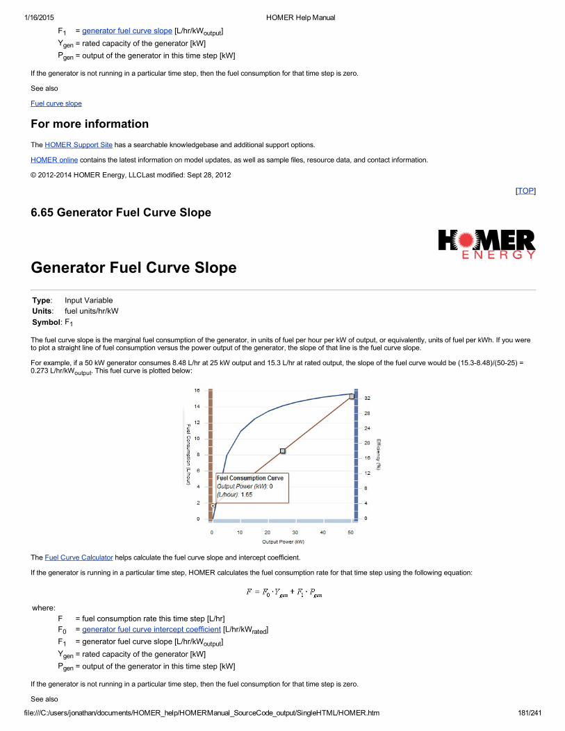
1/16/2015 HOMER Help Manual
file:///C:/users/jonathan/documents/HOMER_help/HOMERManual_SourceCode_output/SingleHTML/HOMER.htm 181/241
F1 = generator fuel curve slope [L/hr/kWoutput]Ygen = rated capacity of the generator [kW]Pgen = output of the generator in this time step [kW]
If the generator is not running in a particular time step, then the fuel consumption for that time step is zero.
See also
Fuel curve slope
For more informationThe HOMER Support Site has a searchable knowledgebase and additional support options.
HOMER online contains the latest information on model updates, as well as sample files, resource data, and contact information.
© 20122014 HOMER Energy, LLCLast modified: Sept 28, 2012
[TOP]
6.65 Generator Fuel Curve Slope
Generator Fuel Curve Slope
Type: Input VariableUnits: fuel units/hr/kWSymbol: F1
The fuel curve slope is the marginal fuel consumption of the generator, in units of fuel per hour per kW of output, or equivalently, units of fuel per kWh. If you wereto plot a straight line of fuel consumption versus the power output of the generator, the slope of that line is the fuel curve slope.
For example, if a 50 kW generator consumes 8.48 L/hr at 25 kW output and 15.3 L/hr at rated output, the slope of the fuel curve would be (15.38.48)/(5025) =0.273 L/hr/kWoutput. This fuel curve is plotted below:
The Fuel Curve Calculator helps calculate the fuel curve slope and intercept coefficient.
If the generator is running in a particular time step, HOMER calculates the fuel consumption rate for that time step using the following equation:
where:F = fuel consumption rate this time step [L/hr]F0 = generator fuel curve intercept coefficient [L/hr/kWrated]F1 = generator fuel curve slope [L/hr/kWoutput]Ygen = rated capacity of the generator [kW]Pgen = output of the generator in this time step [kW]
If the generator is not running in a particular time step, then the fuel consumption for that time step is zero.
See also

1/16/2015 HOMER Help Manual
file:///C:/users/jonathan/documents/HOMER_help/HOMERManual_SourceCode_output/SingleHTML/HOMER.htm 182/241
Fuel curve intercept coefficient
For more informationThe HOMER Support Site has a searchable knowledgebase and additional support options.
HOMER online contains the latest information on model updates, as well as sample files, resource data, and contact information.
© 20122014 HOMER Energy, LLCLast modified: Sept 28, 2012
[TOP]
6.66 Generator Heat Recovery Ratio (PRO)
Generator Heat Recovery Ratio
Type: Input VariableUnits: %Symbol: fhr
This input is relevant only for cogeneration systems, also called combinedheatandpower systems or CHP systems. Such systems serve both electric and thermalloads, with waste heat recovered from the generator meeting some or all of the thermal load. If you do not want to model a cogeneration system, leave this input atzero.
HOMER assumes that the generator converts all of the energy of the fuel into electricity and heat. The generator's fuel curve specifies how much electricity itproduces for a given fuel input, and HOMER simply assumes the remaining fuel energy is converted to heat. The heat recovery ratio is the percentage of that heatthat can be recovered to serve the thermal load.
For more informationThe HOMER Support Site has a searchable knowledgebase and additional support options.
HOMER online contains the latest information on model updates, as well as sample files, resource data, and contact information.
© 20122014 HOMER Energy, LLCLast modified: Sept 28, 2012
[TOP]
6.67 Generator Hourly Replacement Cost
Generator Hourly Replacement Cost
Type: Intermediate VariableUnits: $/hrSymbol: crep,gen
The generator lifetime is specified in number of operating hours. So the hourly replacement cost of each generator can be calculated according to the followingequation:
where:Crep,gen = generator replacement costRgen,h = generator lifetime
For more informationThe HOMER Support Site has a searchable knowledgebase and additional support options.

1/16/2015 HOMER Help Manual
file:///C:/users/jonathan/documents/HOMER_help/HOMERManual_SourceCode_output/SingleHTML/HOMER.htm 183/241
HOMER online contains the latest information on model updates, as well as sample files, resource data, and contact information.
© 20122014 HOMER Energy, LLCLast modified: May 6, 2004
[TOP]
6.68 Generator Lifetime
Generator Lifetime
Type: Input VariableUnits: hrSymbol: Rgen,h
Unlike the lifetime inputs for most other components, the generator lifetime is specified not in years but in hours of operation. This is because the lifetime of agenerator depends strongly on the hours of operation, but not very strongly on its age.
It is not always easy to obtain lifetime data for a particular generator, as it can depend on operating conditions, maintenance frequency, fuel quality, and otherfactors. But it is possible to estimate longevity based on the engine type. Reciprocating internal combustion engines are the most common engine type. Of these,compressionignition (diesel) engines tend to last several times longer than sparkignition engines (gasoline, propane, or natural gas) engines. For longevity, lowspeed (1800 RPM) is superior to high speed (3600 RPM), liquid cooling is superior to air cooling, and pressurized oil lubrication is superior to splash lubrication.The following table serves as a rough guideline for estimating the lifetime of certain types of generators.
Generator TypeSizeRange(kW)
EstimatedLifetime(hrs)
High speed (3600 RPM) aircooledgasoline, natural gas, or propanegenerator
110 250 1,000
High speed (3600 RPM) aircooled diesel 4 20 6,000 10,000
Low speed (1800 RPM) liquidcoolednatural gas or propane generator 15 50 6,000
10,000
Prime power liquidcooled diesel 7 10,000
20,000 80,000
Natural gas microturbine 25 500 50,000 80,000
Because its lifetime is specified in operating hours, the more frequently the generator operates, the shorter its lifetime in years. This affects the economics of thesystem because more frequent replacements leads to higher annualized cost. HOMER takes this into consideration when deciding whether to operate a generatoror to use an alternative dispatchable source such as a battery, the grid, or another generator.
Once it has simulated a system, HOMER calculates the generator's expected lifetime in years and reports it as the generator operational life on the SimulationResults window.
For more informationThe HOMER Support Site has a searchable knowledgebase and additional support options.
HOMER online contains the latest information on model updates, as well as sample files, resource data, and contact information.
© 20122014 HOMER Energy, LLCLast modified: Sept 28, 2012
[TOP]
6.69 Generator Minimum Fossil Fraction (PRO)
Generator Minimum Fossil Fraction
Type: Input Variable

1/16/2015 HOMER Help Manual
file:///C:/users/jonathan/documents/HOMER_help/HOMERManual_SourceCode_output/SingleHTML/HOMER.htm 184/241
Units: %Symbol:
The minimum allowable fossil fraction for a cofired generator operating on a mixture of fossil fuel and biogas. Diesel engines require a certain minimum amount ofdiesel fuel to ensure proper ignition. Sparkignition engines may not have any such requirement, and may be able to operate on pure biogas.
For more informationThe HOMER Support Site has a searchable knowledgebase and additional support options.
HOMER online contains the latest information on model updates, as well as sample files, resource data, and contact information.
© 20122014 HOMER Energy, LLCLast modified: Sept 28, 2012
[TOP]
6.70 Generator Minimum Percent Load
Generator Minimum Percent Load
Type: Input VariableUnits: %Symbol: fgen,min
The minimum allowable load on the generator, as a percentage of its rated capacity. Specifying a minimum load will not prevent the generator from being shut off, itwill simply prevent it from operating at too low a load. This input exists because some manufacturers recommend that their generators not be run below a certainload.
As an example, say this number is set to 30%. If the required power from the generator is 40% of its capacity, it will run at 40%. If the required power is 15%, it willrun at 30%, with the excess power either serving the deferrable load, charging the batteries, or being dumped. If no power is required from the generator, it will beshut off.
For more informationThe HOMER Support Site has a searchable knowledgebase and additional support options.
HOMER online contains the latest information on model updates, as well as sample files, resource data, and contact information.
© 20122014 HOMER Energy, LLCLast modified: Sept 28, 2012
[TOP]
6.71 Generator Nitrogen Oxides Emissions Factor
Generator Nitrogen Oxides Emissions Factor
Type: Input VariableUnits: grams per unit fuel (fuel units can be L, m3, or kg)Symbol: fgen,NOx
The amount of nitrogen oxides emitted per unit fuel consumed by the generator. The actual quantity of this pollutant produced by the generator will depend onengine design and operating conditions, principally the power output of the generator. But HOMER makes a simplifying assumption that this factor is constant.
The following graph shows the value of the nitrogen oxides emissions factor for diesel generators in the size range 50 kW 450 kW. The source of these data is anunpublished NREL report by Erin Kassoy entitled "Modeling diesel exhaust emissions in diesel retrofits". HOMER's default value for the generator's nitrogen oxidesemissions factor is equal to the average value between 50% and 100% load.

1/16/2015 HOMER Help Manual
file:///C:/users/jonathan/documents/HOMER_help/HOMERManual_SourceCode_output/SingleHTML/HOMER.htm 185/241
HOMER uses this value to calculate the emissions of nitrogen oxides. For details, see the article on How HOMER calculates emissions.
For more informationThe HOMER Support Site has a searchable knowledgebase and additional support options.
HOMER online contains the latest information on model updates, as well as sample files, resource data, and contact information.
© 2012 HOMER Energy, LLCLast modified: Sept 28, 2012
[TOP]
6.72 Generator Operational Life
Generator Operational Life
Type: Output Variable
Units: yrSymbol: Rgen
In HOMER, the lifetime of generators is specified in terms of operating hours. The number of years that a generator will last is therefore an output variable, whichHOMER calculates according to the following equation:
where:Rgen,h = generator lifetime [hr]Ngen = the number of hours the generator operates during one year [hr/yr]
For example, if the generator has a lifetime of 20,000 operating hours and HOMER determines that it will operate 4300 hours per year, then its expected lifetime inyears would be 20,000 hours / 4300 hours per year = 4.65 years
For more informationThe HOMER Support Site has a searchable knowledgebase and additional support options.
HOMER online contains the latest information on model updates, as well as sample files, resource data, and contact information.
© 20122014 HOMER Energy, LLCLast modified: Sept 28, 2012
[TOP]
6.73 Generator Particulate Matter Emissions Factor

1/16/2015 HOMER Help Manual
file:///C:/users/jonathan/documents/HOMER_help/HOMERManual_SourceCode_output/SingleHTML/HOMER.htm 186/241
Generator Particulate Matter Emissions Factor
Type: Input VariableUnits: grams per unit fuel (fuel units can be L, m3, or kg)Symbol: fgen,PM
The amount of particulate matter (smoke, soot, and liquid droplets)emitted per unit fuel consumed by the generator. The actual quantity of this pollutant producedby the generator will depend on the fuel, engine design, and operating conditions, including the power output of the generator. But HOMER makes a simplifyingassumption that this factor is constant.
The following graph shows the value of the particulate matter emissions factor for diesel generators in the size range 50 kW 450 kW. The source of these data isan internal NREL report by Erin Kassoy entitled "Modeling diesel exhaust emissions in diesel retrofits". HOMER's default value for the generator's particulatematter emissions factor is equal to the average value between 50% and 100% load.
HOMER uses this value to calculate the emissions of particulate matter. For details, see the article on How HOMER calculates emissions.
For more informationThe HOMER Support Site has a searchable knowledgebase and additional support options.
HOMER online contains the latest information on model updates, as well as sample files, resource data, and contact information.
© 2012 HOMER Energy, LLCLast modified: Sept 28, 2012
[TOP]
6.74 Generator Proportion of Sulfur Emitted as Particulate Matter
Generator Proportion of Sulfur Emitted as ParticulateMatter
Type: Input VariableUnits: %Symbol: xPM
The fraction of the sulfur in the fuel that gets emitted as particulate matter. HOMER assumes that the rest gets emitted as sulfur dioxide. This value is 2.2% fordiesel generators, according to the EPA document EPA420P02016, dated November 2002, entitled "Exhaust and Crankcase Emission Factors for NonroadEngine Modeling CompressionIgnition".
HOMER uses this value to calculate the emissions of sulfur dioxide. Note that HOMER does not use this value this value to calculate emissions of particulatematter. For that, it uses the particulate matter emissions factor. For details, see the article on How HOMER calculates emissions.

1/16/2015 HOMER Help Manual
file:///C:/users/jonathan/documents/HOMER_help/HOMERManual_SourceCode_output/SingleHTML/HOMER.htm 187/241
For more informationThe HOMER Support Site has a searchable knowledgebase and additional support options.
HOMER online contains the latest information on model updates, as well as sample files, resource data, and contact information.
© 20122014 HOMER Energy, LLCLast modified: Sept 28, 2012
[TOP]
6.75 Generator Unburned Hydrocarbons Emissions Factor
Generator Unburned Hydrocarbons Emissions Factor
Type: Input VariableUnits: grams per unit fuel (fuel units can be L, m3, or kg)Symbol: fgen,UHC
The amount of unburned hydrocarbons emitted per unit fuel consumed by the generator. The actual quantity of this pollutant produced by the generator will dependon the fuel, engine design, and operating conditions, including the power output of the generator. But HOMER makes a simplifying assumption that this factor isconstant.
The following graph shows the value of the unburned hydrocarbons emissions factor for diesel generators in the size range 50 kW 450 kW. The source of thesedata is an internal NREL report by Erin Kassoy entitled "Modeling diesel exhaust emissions in diesel retrofits". The default value for the generator's unburnedhydrocarbon emissions factor is equal to the average value between 50% and 100% load.
HOMER uses this value to calculate the emissions of unburned hydrocarbons and carbon dioxide. For details, see the article on How HOMER calculatesemissions.
For more informationThe HOMER Support Site has a searchable knowledgebase and additional support options.
HOMER online contains the latest information on model updates, as well as sample files, resource data, and contact information.
© 20122014 HOMER Energy, LLCLast modified: Sept 28, 2012
[TOP]
6.76 Grid Costs
Grid Costs
1/16/2015 HOMER Help Manual
file:///C:/users/jonathan/documents/HOMER_help/HOMERManual_SourceCode_output/SingleHTML/HOMER.htm 188/241
Since the grid is unlike any other component, HOMER calculates the costs associated with the grid in a unique way. This article explains how HOMER calculateseach of the grid cost outputs.
Grid capital costIf the system is connected to the grid and contains some other power producing device (such as a microturbine, a fuel cell, a PV array, or a wind turbine), the gridcapital cost is equal to the interconnection charge. Otherwise, the grid capital cost is zero.
Grid replacement costThe replacement cost of the grid is always zero.
Grid O&M costThe grid O&M cost is equal to the annual cost of buying electricity from the grid (energy cost plus demand cost) minus any income from the sale of electricity to thegrid. For gridconnected systems that contain some other power producing device (such as a microturbine, a fuel cell, a PV array, or a wind turbine), the grid O&Mcost also includes the standby charge.
See also
Interconnection charge
Standby charge
Capital recovery factor
Project lifetime
For more informationThe HOMER Support Site has a searchable knowledgebase and additional support options.
HOMER online contains the latest information on model updates, as well as sample files, resource data, and contact information.
© 20122014 HOMER Energy, LLCLast modified: Sept 28, 2012
[TOP]
6.77 Grid Interconnection Charge (PRO)
Grid Interconnection Charge
Type: Input VariableUnits: $Symbol: Cgrid,int
The interconnection charge is a onetime fee charged by the utility for allowing a power system to be connected to the grid. HOMER does not apply this fee to gridonly systems, but rather to gridconnected systems that include some other generation source. For such systems, the interconnection charge is added to the gridcapital cost.
See also:
Standby charge
Grid capital cost
For more informationThe HOMER Support Site has a searchable knowledgebase and additional support options.
HOMER online contains the latest information on model updates, as well as sample files, resource data, and contact information.
© 20122014 HOMER Energy, LLCLast modified: Sept 28, 2012
[TOP]
6.78 Grid Standby Charge (PRO)

1/16/2015 HOMER Help Manual
file:///C:/users/jonathan/documents/HOMER_help/HOMERManual_SourceCode_output/SingleHTML/HOMER.htm 189/241
Grid Standby Charge
Type: Input VariableUnits: $/yrSymbol: Cgrid,standby
The standby charge is an annual fee charged by the utility for providing backup grid power for a gridconnected power system. HOMER does not apply this fee togridonly systems, but rather to gridconnected systems that include some other generation source (like a microturbine, a fuel cell, or a PV array). For suchsystems, the standby charge is added to the grid O&M cost.
See also:
Interconnection charge
Grid O&M cost
For more informationThe HOMER Support Site has a searchable knowledgebase and additional support options.
HOMER online contains the latest information on model updates, as well as sample files, resource data, and contact information.
© 20122014 HOMER Energy, LLCLast modified: Sept 28, 2012
[TOP]
6.79 Ground Reflectance
Ground Reflectance
Type: Input VariableUnits: %Symbol: rg
The ground reflectance (also called albedo) is the fraction of solar radiation incident on the ground that is reflected. A typical value for grasscovered areas is 20%.Snowcovered areas may have a reflectance as high as 70%. This value is used in calculating the radiation incident on the tilted PV panels, but it has only amodest effect.
See also:
PV Inputs window
For more informationThe HOMER Support Site has a searchable knowledgebase and additional support options.
HOMER online contains the latest information on model updates, as well as sample files, resource data, and contact information.
© 20122014 HOMER Energy, LLCLast modified: Sept 28, 2012
[TOP]
6.80 Hydrocarbons Emissions Penalty (PRO)
Hydrocarbons Emissions Penalty

1/16/2015 HOMER Help Manual
file:///C:/users/jonathan/documents/HOMER_help/HOMERManual_SourceCode_output/SingleHTML/HOMER.htm 190/241
Type: Input VariableUnits: $/tSymbol: cHC
Use the HC emissions penalty to penalize systems for their production of unburned hydrocarbons. HOMER uses this input value when calculating the Other O&Mcost.
For more informationThe HOMER Support Site has a searchable knowledgebase and additional support options.
HOMER online contains the latest information on model updates, as well as sample files, resource data, and contact information.
© 20122014 HOMER Energy, LLCLast modified: Sept 28, 2012
[TOP]
6.81 Hour of Peak Windspeed
Hour of Peak Windspeed
Type: Input VariableUnits: noneSymbol: fTypical Range: 14 16
The hour of peak windspeed is the hour of the day that tends to be the windiest, on average. The article on diurnal pattern strength describes how HOMERcalculates this value.
We calculated the hour of peak wind speed for each of the 239 weather stations in the TMY2 data set. The histogram below shows the resulting distribution. Youcan see the measured values themselves in the table of measured wind parameters.
See also
Diurnal pattern strength
Autocorrelation factor
Weibull k
For more informationThe HOMER Support Site has a searchable knowledgebase and additional support options.
HOMER online contains the latest information on model updates, as well as sample files, resource data, and contact information.
© 2012 HOMER Energy, LLCLast modified: Sept 28, 2012
[TOP]
6.82 Hydro Turbine Efficiency (PRO)

1/16/2015 HOMER Help Manual
file:///C:/users/jonathan/documents/HOMER_help/HOMERManual_SourceCode_output/SingleHTML/HOMER.htm 191/241
Hydro Turbine Efficiency
Type: Input VariableUnits: %Symbol: hhyd
The efficiency with which the hydro turbine converts the mechanical power of the water into electrical power. HOMER uses this value to calculate the nominalhydro power and the actual output power of hydro turbine in each time step.
See also
Nominal hydro power
Calculating hydro power output
For more informationThe HOMER Support Site has a searchable knowledgebase and additional support options.
HOMER online contains the latest information on model updates, as well as sample files, resource data, and contact information.
© 20122014 HOMER Energy, LLCLast modified: Sept 28, 2012
[TOP]
6.83 Hydro Turbine Flow Rate (PRO)
Hydro Turbine Flow Rate
Type: Intermediate VariableUnits: m3/sSymbol:
The hydro turbine flow rate is the amount of water flowing through the hydro turbine. HOMER calculates this value in each time step using the following equation:
where:
= the flow rate available to the hydro turbine [m3/s]= minimum flow rate of the hydro turbine [m3/s]= maximum flow rate of the hydro turbine [m3/s]
Note: As this equation shows, HOMER assumes that unless the available stream exceeds the turbine's minimum flow rate, the turbine flow rate is zero, meaningthe turbine does not operate and hence produces no power. If HOMER reports that your hydro turbine is not producing any power, this is probably the reason.
HOMER uses the hydro turbine flow rate to calculate the hydro power output in each time step.
See also
Calculating the hydro power output
For more informationThe HOMER Support Site has a searchable knowledgebase and additional support options.
HOMER online contains the latest information on model updates, as well as sample files, resource data, and contact information.
© 20122014 HOMER Energy, LLCLast modified: December 27, 2007
[TOP]

1/16/2015 HOMER Help Manual
file:///C:/users/jonathan/documents/HOMER_help/HOMERManual_SourceCode_output/SingleHTML/HOMER.htm 192/241
6.84 Hydrogen Tank Autonomy (PRO)
Hydrogen Tank Autonomy
Type: Output VariableUnits: hrSymbol: Ahtank
The hydrogen tank autonomy is the ratio of the energy capacity of the hydrogen tank to the electric load. HOMER calculates the hydrogen tank autonomy using thefollowing equation:
where:Yhtank = capacity of the hydrogen tank [kg]LHVH2 = energy content (lower heating value) of hydrogen [120 MJ/kg]Lprim,ave = average primary load [kWh/d]
For more informationThe HOMER Support Site has a searchable knowledgebase and additional support options.
HOMER online contains the latest information on model updates, as well as sample files, resource data, and contact information.
© 20122014 HOMER Energy, LLCLast modified: Sept 28, 2012
[TOP]
6.85 Initial Capital Cost
Initial Capital Cost
The initial capital cost of a component is the total installed cost of that component at the beginning of the project.
Tip: To see initial capital costs and all other costs that occur over the lifetime of the project, see the Cash Flow Details Table.
See also
Replacement cost
Cash Flow Details table
For more informationThe HOMER Support Site has a searchable knowledgebase and additional support options.
HOMER online contains the latest information on model updates, as well as sample files, resource data, and contact information.
© 20122014 HOMER Energy, LLCLast modified: September 16, 2009
[TOP]
6.86 Interest Rate
Interest Rate

1/16/2015 HOMER Help Manual
file:///C:/users/jonathan/documents/HOMER_help/HOMERManual_SourceCode_output/SingleHTML/HOMER.htm 193/241
Type: Input VariableUnits: %Symbol: i
The interest rate that one enters for HOMER's input is the annual real interest rate (also called the real interest rate or just interest rate). It is the discount rate usedto convert between onetime costs and annualized costs. HOMER uses the interest rate to calculate discount factors and to calculate annualized costs from netpresent costs.
You enter the interest rate in the Economic Inputs window.
To calcualte the annual real interest rate from the nominal interest rate, use the following equation:
where:i = real interest ratei' = nominal interest rate (the rate at which you could borrow money)f = annual inflation rate
For example, if the nominal interest rate is 8% and the inflation rate is 3.5%, the annual real interest rate is 4.35%.
By defining the interest rate in this way, inflation is factored out of the economic analysis. All costs therefore become real costs, meaning that they are in defined interms of constant dollars. The assumption is that the rate of inflation is the same for all costs.
See also
Economic Inputs window
Annualized cost
Net present cost
Salvage value
Interest rate
For more informationThe HOMER Support Site has a searchable knowledgebase and additional support options.
HOMER online contains the latest information on model updates, as well as sample files, resource data, and contact information.
© 20122014 HOMER Energy, LLCLast modified: Sept 28, 2012
[TOP]
6.87 Levelized Cost of Energy
Levelized Cost of Energy
Type: Output VariableUnits: $/kWhSymbol: COE
HOMER defines the levelized cost of energy (COE) as the average cost per kWh of useful electrical energy produced by the system. To calculate the COE,HOMER divides the annualized cost of producing electricity (the total annualized cost minus the cost of serving the thermal load) by the total electric load seved,using the following equation:
where:Cann,tot = total annualized cost of the system [$/yr]cboiler = boiler marginal cost [$/kWh]Hserved = total thermal load served [kWh/yr]Eserved = total electrical load served [kWh/yr]

1/16/2015 HOMER Help Manual
file:///C:/users/jonathan/documents/HOMER_help/HOMERManual_SourceCode_output/SingleHTML/HOMER.htm 194/241
The second term in the numerator is the portion of the annualized cost that results from serving the thermal load. In systems that do not serve a thermal load(Hthermal=0) this term will equal zero.
The COE is a convenient metric with which to compare systems, but HOMER does not rank systems based on COE. For an explanation, please refer to Why doesHOMER rank systems by total NPC?
See also
Annualized cost
Total annualized cost
Why does HOMER rank systems by total NPC?
For more informationThe HOMER Support Site has a searchable knowledgebase and additional support options.
HOMER online contains the latest information on model updates, as well as sample files, resource data, and contact information.
© 20122014 HOMER Energy, LLCLast modified: Sept 28, 2012
[TOP]
6.88 Lifetime Throughput
Lifetime Throughput
Type: Input VariableUnits: kWhSymbol: Qlifetime
If the battery properties indicate that the battery life is limited by throughput, HOMER assumes that the battery will require replacement after a fixed amount ofenergy cycles through the battery, regardless of the depth of the individual chargedischarge cycles. HOMER uses this lifetime battery throughput to calculate thelife of the battery bank and the battery wear cost.
See also
Battery float life
Create New Battery window
For more informationThe HOMER Support Site has a searchable knowledgebase and additional support options.
HOMER online contains the latest information on model updates, as well as sample files, resource data, and contact information.
© 20122014 HOMER Energy, LLCLast modified: Sept 28, 2012
[TOP]
6.89 Load Factor
Load Factor
The load factor is a dimensionless number equal to the average load divided by the peak load.
Example: If the average load is 66 kWh/d (or 2.75 kW) and the peak load is 10.5 kW, the load factor is 2.75 kW / 10.5 kW = 0.26.
For more informationThe HOMER Support Site has a searchable knowledgebase and additional support options.
HOMER online contains the latest information on model updates, as well as sample files, resource data, and contact information.

1/16/2015 HOMER Help Manual
file:///C:/users/jonathan/documents/HOMER_help/HOMERManual_SourceCode_output/SingleHTML/HOMER.htm 195/241
© 20122014 HOMER Energy, LLCLast modified: July 28, 2004
[TOP]
6.90 Load Following Strategy
Load Following Strategy
The load following strategy is a dispatch strategy whereby whenever a generator operates, it produces only enough power to meet the primary load. Lowerpriorityobjectives such as charging the battery bank or serving the deferrable load are left to the renewable power sources.
Under the load following strategy, HOMER dispatches the system's controllable power sources (generators, grid, battery bank) so as to serve the primary load andthe thermal load at the least total cost each time step, while satisfying the operating reserve requirement. The total cost includes the cost of fuel, operation andmaintenance, and replacement. To accomplish this, HOMER calculates the fixed and marginal cost of each dispatchable power source:
A generator's fixed cost is equal to its hourly operation and maintenance cost plus its hourly replacement cost plus the cost of its noload fuel consumption. Itsmarginal cost is equal to its fuel curve slope times the fuel price. If waste heat can be recovered from the generator and the waste heat is needed to servethe thermal load, the generator's marginal cost is reduced by the value of the thermal energy it produces (which is equal to the marginal cost of thermalenergy from the boiler). If a cost is assigned to carbon emissions, the generator's marginal cost is increased accordingly.The battery bank's fixed cost is zero and its marginal cost is equal to the battery wear cost.The grid's fixed cost is zero and its marginal cost is equal to the grid power price. If a cost is assigned to carbon emissions, the grid's marginal cost isincreased accordingly.
Once it characterizes each dispatchable source in this way, HOMER searches for the combination of generation sources that satisfies the primary load, requiredoperating reserve, and thermal load at least cost.
See also
Cycle charging strategy
For more informationThe HOMER Support Site has a searchable knowledgebase and additional support options.
HOMER online contains the latest information on model updates, as well as sample files, resource data, and contact information.
© 20122014 HOMER Energy, LLCLast modified: May 6, 2004
[TOP]
6.91 Maximum Annual Capacity Shortage
Maximum Annual Capacity Shortage
Type: Input VariableUnits: %
The maximum annual capacity shortage is the maximum allowable value of the capacity shortage fraction, which is the total capacity shortage divided by the totalelectric load. HOMER considers infeasible (or unacceptable) any system with a higher value of the capacity shortage fraction.
Allowing some capacity shortage can change the results dramatically in some cases. This might happen if there were a very high peak for a very short time. If themaximum annual capacity shortage is set to zero, HOMER will size the system to meet even this very high peak load. This could mean that the system has toinclude large, expensive equipment that is not fully used most of the time. If you allow a small amount of capacity shortage, HOMER could choose to install smaller,less expensive equipment that would be able to supply all but that peak load.
Note: If you set each of the four operating reserve inputs to zero, the capacity shortage fraction will be equal to the unmet load fraction.
See also:
Required operating reserve
Total capacity shortage
Capacity shortage fraction
Unmet load fraction
For more information

1/16/2015 HOMER Help Manual
file:///C:/users/jonathan/documents/HOMER_help/HOMERManual_SourceCode_output/SingleHTML/HOMER.htm 196/241
The HOMER Support Site has a searchable knowledgebase and additional support options.
HOMER online contains the latest information on model updates, as well as sample files, resource data, and contact information.
© 20122014 HOMER Energy, LLCLast modified: Sept 28, 2012
[TOP]
6.92 Maximum Battery Capacity
Maximum Battery Capacity
The maximum capacity (or theoretical capacity) of a battery is the total amount of energy it contains when fully charged. It is not possible to extract all this energy atany finite discharge current (it would take an infinite amount of time to extract it all), so battery sizes are not typically given in terms of maximum capacity. HOMERcalculates the maximum capacity for use in the kinetic battery model.
See also
Nominal Capacity
For more informationThe HOMER Support Site has a searchable knowledgebase and additional support options.
HOMER online contains the latest information on model updates, as well as sample files, resource data, and contact information.
© 20122014 HOMER Energy, LLCLast modified: May 6, 2004
[TOP]
6.93 Maximum Flow Rate (PRO)
Maximum Flow Rate
Type: Intermediate VariableUnits: m3/sSymbol:
The maximum flow rate is the maximum allowable flow rate through the hydro turbine. HOMER calculates the maximum flow rate of the hydro turbine using thefollowing equation:
where:wmax = the hydro turbine's maximum flow ratio [%]
= the hydro turbine's design flow rate [m3/s]
HOMER uses this value to calculate the hydro turbine flow rate in each time step.
See also
Minimum flow rate
Hydro turbine flow rate
Calculating the hydro power output
For more informationThe HOMER Support Site has a searchable knowledgebase and additional support options.
HOMER online contains the latest information on model updates, as well as sample files, resource data, and contact information.
© 2012 HOMER Energy, LLCLast modified: December 27, 2007
[TOP]

1/16/2015 HOMER Help Manual
file:///C:/users/jonathan/documents/HOMER_help/HOMERManual_SourceCode_output/SingleHTML/HOMER.htm 197/241
6.94 Maximum Flow Ratio (PRO)
Maximum Flow Ratio
Type: Input VariableUnits: %
Symbol: wmax
The maximum acceptable flow rate through the hydro turbine, expressed as a percentage of the turbine's design flow rate. HOMER uses this input to calculate themaximum flow rate through the hydro turbine, and hence the actual flow rate through the hydro turbine.
See also
Design flow rate
Maximum flow rate
Hydro turbine flow rate
Minimum flow ratio
For more informationThe HOMER Support Site has a searchable knowledgebase and additional support options.
HOMER online contains the latest information on model updates, as well as sample files, resource data, and contact information.
© 20122014 HOMER Energy, LLCLast modified: Sept 28, 2012
[TOP]
6.95 Purchase Capacity
Purchase Capacity
Type: Input VariableUnits: kWSymbol: Tgrid
The purchase capacity is the maximum amount of power that can be drawn from the grid at any time. It is a decision variable because of the effect of demandcharges. HOMER does not explicitly consider the demand rate in its timestepbytimestep decisions at to how to control the power system; the demand charge issimply calculated at the end of each annual simulation. As a result, HOMER will not turn on a generator simply to save demand charges. But it will turn on agenerator whenever the load exceeds the maximum grid demand.
If the demand rate is zero, you need only specify a single value for the maximum grid demand. Normally, the true capacity of the grid is much higher than thesystem peak load, and the maximum grid demand can be set to any value higher than the system peak load. In the rare case that the grid is unable to meet thesystem peak load, the maximum grid demand should be set to the actual capacity of the grid.
If the demand rate is not zero, specify a value equal to or greater than the peak load, plus at least one value smaller than the peak load. HOMER will find theoptimal value.
The maximum grid demand appears in a table on the Grid Inputs window:
For more informationThe HOMER Support Site has a searchable knowledgebase and additional support options.

1/16/2015 HOMER Help Manual
file:///C:/users/jonathan/documents/HOMER_help/HOMERManual_SourceCode_output/SingleHTML/HOMER.htm 198/241
HOMER online contains the latest information on model updates, as well as sample files, resource data, and contact information.
© 20122014 HOMER Energy, LLCLast modified: Sept 28, 2012
[TOP]
6.96 Minimum Flow Rate (PRO)
Minimum Flow Rate
Type: Intermediate VariableUnits: m3/sSymbol:
The minimum flow rate is the minimum allowable flow rate through the hydro turbine. HOMER assumes that the hydro turbine can operate only if the availablestream flow is equal to or exceeds this minimum value. HOMER calculates the minimum flow rate of the hydro turbine using the following equation:
where:wmin = the hydro turbine's minimum flow ratio [%]
= the hydro turbine's design flow rate [m3/s]
HOMER uses this value to calculate the hydro turbine flow rate in each time step.
See also
Maximum flow rate
Hydro turbine flow rate
Calculating the hydro power output
For more informationThe HOMER Support Site has a searchable knowledgebase and additional support options.
HOMER online contains the latest information on model updates, as well as sample files, resource data, and contact information.
© 2012 HOMER Energy, LLCLast modified: December 27, 2007
[TOP]
6.97 Minimum Flow Ratio (PRO)
Minimum Flow Ratio
Type: Input VariableUnits: %Symbol: wmin
The minimum acceptable flow rate through the hydro turbine, expressed as a percentage of the turbine's design flow rate. HOMER uses this input to calculate theminimum flow rate through the hydro turbine, and hence the actual flow rate through the hydro turbine.
See also
Design flow rate
Minimum flow rate
Hydro turbine flow rate
Maximum flow ratio

1/16/2015 HOMER Help Manual
file:///C:/users/jonathan/documents/HOMER_help/HOMERManual_SourceCode_output/SingleHTML/HOMER.htm 199/241
For more informationThe HOMER Support Site has a searchable knowledgebase and additional support options.
HOMER online contains the latest information on model updates, as well as sample files, resource data, and contact information.
© 20122014 HOMER Energy, LLCLast modified: Sept 28, 2012
[TOP]
6.98 Net Present Cost
Net Present Cost
The net present cost (or lifecycle cost) of a component is the present value of all the costs of installing and operating that component over the project lifetime,minus the present value of all the revenues that it earns over the project lifetime. HOMER calculates the net present cost of each component of the system, and ofthe system as a whole.
Tip: To calculate net present costs, HOMER performs a cash flow analysis. You can see the resulting table of nominal and discounted cash flows in the Cash FlowDetails Table.
Example: A diesel generator has an initial capital cost of $96,000, a replacement cost of $48,000, and a lifetime of 3.52 years. Its cost of operation andmaintenance (O&M) is $2,471/yr, and its fuel cost is $34,969/yr. What is the net present cost of this generator over a 25year project lifetime at an annual realinterest rate of 6%?
To perform this calculation, HOMER produces a cash flow table such as the one that appears below. Except for the salvage value that occurs at the end of the25th year, all of these cash flows are costs, so they appear as negative numbers in the table.
The first column shows the time at which each cash flow occurs, in years since the start of the project. The capital cost occurs at the start of the project, meaningyear zero. The annual O&M and fuel costs occur at the end of each year, and the replacement costs happen every 3.52 years.
The second column, highlighted in yellow, contains the discount factor. The columns highlighted in green contain the nominal cash flows, and the columnshighlighted in purple contain the same cash flow discounted to year zero. HOMER calculates the discounted costs by multiplying the nominal costs by the discountfactor.
The bottom row below the purple discounted cash flow columns contains the net present value of each category of cash flow, as well as the total net present value,shown in red, with a value of $725,240. The net present value and the net present cost differ only in sign, so the net present cost of this generator over the 25yearproject lifetime is $725,240.
HOMER does a similar analysis for each component of the system, and for the system as a whole.
Year Discount Nominal Cash Flows Discounted Cash Flows
Factor Capital Replacement Salvage O&M Fuel Total Capital Replacement Salvage O&M Fuel Total0 1.000 96,000 96,000 96,000 96,0001 0.943 2,471 34,969 37,441 2,331 32,990 35,3212 0.890 2,471 34,969 37,441 2,200 31,123 33,3223 0.840 2,471 34,969 37,441 2,075 29,361 31,436
3.52 0.815 48,000 48,000 39,098 39,0984 0.792 2,471 34,969 37,441 1,958 27,699 29,6575 0.747 2,471 34,969 37,441 1,847 26,131 27,9786 0.705 2,471 34,969 37,441 1,742 24,652 26,3947 0.665 2,471 34,969 37,441 1,644 23,257 24,900
7.04 0.663 48,000 48,000 31,847 31,8478 0.627 2,471 34,969 37,441 1,551 21,940 23,4919 0.592 2,471 34,969 37,441 1,463 20,698 22,16110 0.558 2,471 34,969 37,441 1,380 19,527 20,907
10.56 0.540 48,000 48,000 25,941 25,94111 0.527 2,471 34,969 37,441 1,302 18,421 19,72312 0.497 2,471 34,969 37,441 1,228 17,379 18,60713 0.469 2,471 34,969 37,441 1,159 16,395 17,55414 0.442 2,471 34,969 37,441 1,093 15,467 16,560
14.08 0.440 48,000 48,000 21,130 21,13015 0.417 2,471 34,969 37,441 1,031 14,592 15,62316 0.394 2,471 34,969 37,441 973 13,766 14,73817 0.371 2,471 34,969 37,441 918 12,986 13,904
17.60 0.359 48,000 48,000 17,212 17,21218 0.350 2,471 34,969 37,441 866 12,251 13,117

1/16/2015 HOMER Help Manual
file:///C:/users/jonathan/documents/HOMER_help/HOMERManual_SourceCode_output/SingleHTML/HOMER.htm 200/241
19 0.331 2,471 34,969 37,441 817 11,558 12,37520 0.312 2,471 34,969 37,441 771 10,904 11,67421 0.294 2,471 34,969 37,441 727 10,286 11,013
21.12 0.292 48,000 48,000 14,020 14,02022 0.278 2,471 34,969 37,441 686 9,704 10,39023 0.262 2,471 34,969 37,441 647 9,155 9,80224 0.247 2,471 34,969 37,441 610 8,637 9,247
24.64 0.238 48,000 48,000 11,420 11,42025 0.233 43,120 2,471 34,969 5,679 10,047 576 8,148 1,323
Total 96,000 336,000 43,120 61,784 874,234 1,324,899 96,000 160,668 10,047 31,593 447,026 725,239
Note that HOMER uses the discount factor to account not for inflation, but for the time value of money. Inflation is factored out of the analysis by the use of the realinterest rate instead of the nominal interest rate. All costs in the table above are in yearzero dollars. This explains why the fuel and O&M costs remain the same foreach year of the project lifetime.
But even when we factor inflation out of the analysis, the time value of money dictates that a future cash flow is worth less than a present cash flow of the sameamount. The discount factor accounts for this effect; its value decreases with increasing number of years from the start of the project.
See also
Total net present cost
Annualized cost
Present value
Future value
Salvage value
Project lifetime
Interest rate
Discount factor
Cash Flow Details table
For more informationThe HOMER Support Site has a searchable knowledgebase and additional support options.
HOMER online contains the latest information on model updates, as well as sample files, resource data, and contact information.
© 20122014 HOMER Energy, LLCLast modified: August 30, 2010
[TOP]
6.99 Nominal Battery Capacity
Nominal Battery Capacity
The nominal capacity (or rated capacity) of a battery is the amount of energy that could be withdrawn from it at a particular constant current, starting from a fullycharged state. The current used to rate batteries varies from one manufacturer to another, but it is typically either the 10hour, 20hour, or 100hour rate. The 10hour rate (C10) is the current that causes the battery to be drained after 10 hours.
See also
Maximum battery capacity
For more informationThe HOMER Support Site has a searchable knowledgebase and additional support options.
HOMER online contains the latest information on model updates, as well as sample files, resource data, and contact information.
© 20122014 HOMER Energy, LLCLast modified: May 6, 2004
[TOP]
6.100 Nominal Hydro Power (PRO)

1/16/2015 HOMER Help Manual
file:///C:/users/jonathan/documents/HOMER_help/HOMERManual_SourceCode_output/SingleHTML/HOMER.htm 201/241
Nominal Hydro Power
Type: Output VariableUnits: kWSymbol: Phyd,nom
The nominal power of the hydro system. This would be the power produced by the hydro turbine given the available head and a stream flow equal to the designflow rate of the hydro turbine. The calculation of the nominal hydro power includes the efficiency of the hydro turbine, but not the pipe head loss.
Note: HOMER uses this value only to identify the size of the hydro system, to allow easy comparison to the sizes of other components of the power system.
HOMER calculates the nominal hydro power using the following equation:
where:Phyd,nom = nominal power output of the hydro turbine [kW]hhyd = hydro turbine efficiency [%]rwater = density of water [1000 kg/m3]g = acceleration due to gravity [9.81 m/s2]h = available head [m]
= the design flow rate of the hydro turbine [m3/s]
See also
Calculating hydro power output
For more informationThe HOMER Support Site has a searchable knowledgebase and additional support options.
HOMER online contains the latest information on model updates, as well as sample files, resource data, and contact information.
© 20122014 HOMER Energy, LLCLast modified: December 27, 2007
[TOP]
6.101 Nonrenewable Electrical Production
Nonrenewable Electrical Production
Type: Intermediate VariableUnits: kWh/yrSymbol: Enonren
The nonrenewable electrical production is the total amount of electrical energy produced annually by the nonrenewable components of the power system. HOMERuses the following equation to calculate the nonrenewable electrical production:
where:Eprod = total electrical production [kWh]Eren = renewable electrical production [kWh]
1/16/2015 HOMER Help Manual
file:///C:/users/jonathan/documents/HOMER_help/HOMERManual_SourceCode_output/SingleHTML/HOMER.htm 202/241
HOMER uses this variable to calculate the renewable fraction.
See also
Renewable fraction
Renewable thermal production
Total electrical production
For more informationThe HOMER Support Site has a searchable knowledgebase and additional support options.
HOMER online contains the latest information on model updates, as well as sample files, resource data, and contact information.
© 20122014 HOMER Energy, LLCLast modified: Sept 28, 2012
[TOP]
6.102 Nonrenewable Thermal Production (PRO)
Nonrenewable Thermal Production
Type: Intermediate VariableUnits: kWh/yrSymbol: Hnonren
The nonrenewable thermal production is the total amount of thermal energy produced annually by nonrenewable thermal energy sources. HOMER uses thefollowing equation to calculate the nonrenewable thermal production:
where:Hprod = total thermal production [kWh]Hren = renewable thermal production [kWh]
HOMER uses this value to calculate the renewable fraction.
See also
Renewable fraction
Renewable electrical production
Total thermal production
For more informationThe HOMER Support Site has a searchable knowledgebase and additional support options.
HOMER online contains the latest information on model updates, as well as sample files, resource data, and contact information.
© 20122014 HOMER Energy, LLCLast modified: Sept 28, 2012
[TOP]
6.103 NOx Emissions Penalty (PRO)
NOx Emissions Penalty
Type: Input Variable

1/16/2015 HOMER Help Manual
file:///C:/users/jonathan/documents/HOMER_help/HOMERManual_SourceCode_output/SingleHTML/HOMER.htm 203/241
Units: $/tSymbol: cNOx
Use the NOx emissions penalty to penalize systems for their production of nitrogen oxides. HOMER uses this input value when calculating the Other O&M cost.
For more informationThe HOMER Support Site has a searchable knowledgebase and additional support options.
HOMER online contains the latest information on model updates, as well as sample files, resource data, and contact information.
© 20122014 HOMER Energy, LLCLast modified: Sept 28, 2012
[TOP]
6.104 O&M (Operation and Maintenance) Cost
O&M (Operation and Maintenance) Cost
The O&M cost of a component is the cost associated with operating and maintaining that component. The total O&M cost of the system is the sum of the O&Mcosts of each system component.
For most components, you enter the O&M cost as an annual amount. In the case of the generator, you enter the O&M cost as an hourly value, and HOMERmultiplies that by the operating hours per year to calculate the annual O&M cost.
The grid O&M cost is the annual cost of buying power from the grid minus any revenue earned from selling power to the grid.
HOMER classifies miscellaneous annual costs, such as the system fixed O&M cost, and penalties such as emissions penalties and the capacity shortage penalty,as other O&M cost.
HOMER displays the O&M costs on the Cost Summary and Cash Flow tabs of the Simulation Results window.
See also
Grid costs
Other O&M cost
System fixed O&M cost
Capacity shortage penalty
Emissions inputs
For more informationThe HOMER Support Site has a searchable knowledgebase and additional support options.
HOMER online contains the latest information on model updates, as well as sample files, resource data, and contact information.
© 20122014 HOMER Energy, LLCLast modified: May 30, 2008
[TOP]
6.105 OneHour Autocorrelation Factor
OneHour Autocorrelation Factor
Type: Input VariableUnits: noneSymbol: r1Typical Range: 0.80 0.95
The autocorrelation factor reflects how strongly the wind speed in one time step depends on the wind speeds in previous time steps. A high autocorrelation factorindicates that the wind speed tends to depend strongly on the wind speed in the previous time step. Lower values indicate that the wind speed tends to fluctuate ina more random fashion from one time step to the next. Among other factors, local topography can influence this parameter . Autocorrelation factors tend to be

1/16/2015 HOMER Help Manual
file:///C:/users/jonathan/documents/HOMER_help/HOMERManual_SourceCode_output/SingleHTML/HOMER.htm 204/241
lower (0.70 0.80) in areas of complex topography and higher (0.90 0.97) in areas of more uniform topography.
To define the autocorrelation factor we first need to look at the typical autocorrelation characteristics of measured wind speed data.
As explained in the discussion of autocorrelation, the daily patterns in the wind data tend to complicate its autocorrelation function. The graph below shows theautocorrelation function for the hourly wind speed data measured at San Diego, California:
To simplify the autocorrelation characteristics of wind data, we can factor out the diurnal pattern. HOMER does this by calculating the average diurnal profile, andthen subtracting that profile from the wind speed data. For example, if the diurnal profile showed an average wind speed of 3.2 m/s at 1 a.m., then HOMER wouldsubtract 3.2 m/s from all 365 values of wind speed at 1 a.m. It does the same for all 24 hours of the day, resulting in a time series that has an average of 0 m/s andno daily pattern. The autocorrelation function of this new time series typically displays almost no oscillation. The graph below shows the autocorrelation function forthe San Diego data data after subtracting out the diurnal profile:
The autocorrelation function shown above dies down roughly in damped exponential fashion, so that to a good approximation,
We can therefore describe the degree of correlation with a single parameter. In HOMER we call this the onehour autocorrelation factor, which is rk where k is thenumber of time steps in one hour. If the time step is 60 minutes, the onehour autocorrelation factor is r1. If the time step is 20 minutes, the onehourautocorrelation factor is r3. If the time step is 10 minutes, the onehour autocorrelation factor is r6.
To help HOMER users estimate the onehour autocorrelation factor in the absence of measured data, we calculated the autocorrelation factor for each of the 239weather stations in the TMY2 data set. The histogram below shows the resulting distribution. You can see the measured values themselves in the table of TMY2wind parameters.
The complexity of local topography has a significant effect on the autocorrelation factor. Areas surrounded by a variety of different types of topography tend to havelow (0.70 0.80) autocorrelation factors. For example, the stations with the lowest autocorrelation factors in the table of measured wind parameters are LosAngeles CA, Denver CO, Phoeniz AZ, Lander WY, Seattle WA, and Salt Lake City UT. Each of these cities is surrounded by complex topography: mountains orhills on one side, and plains or open water on another. In such surroundings, shifts in wind direction can result in the wind having a very different character. Sothere is less persistence of wind speeds, and therefore lower autocorrelation [Brett and Tuller, 1991].
Areas surrounded by more uniform topography tend to have high (0.90 0.97) autocorrelation factors. The stations with the highest autocorrelation factors in thetable of measured wind parameters include Cut Bank MT, St. Paul Island AK, and the island of Guam. Each of these sites is surrounded by relatively featurelesstopography: either plains or open water.
Note: the autocorrelation factor is independent of the Weibull k value. Whereas the Weibull k value reflects the breadth of the annual distribution of wind speeds,the autocorrelation factor reflects how randomly the wind speeds vary from hour to hour. The data contained in the table of measured wind parameters shows nocorrelation between these two parameters.
See also
Autocorrelation
Generating synthetic wind data

1/16/2015 HOMER Help Manual
file:///C:/users/jonathan/documents/HOMER_help/HOMERManual_SourceCode_output/SingleHTML/HOMER.htm 205/241
Weibull k value
Diurnal pattern strength
Hour of peak wind speed
TMY2 wind parameters
For more informationThe HOMER Support Site has a searchable knowledgebase and additional support options.
HOMER online contains the latest information on model updates, as well as sample files, resource data, and contact information.
© 2012 HOMER Energy, LLCLast modified: Sept 28, 2012
[TOP]
6.106 Operating Capacity
Operating Capacity
The operating capacity is the total amount of electrical generation capacity that is operating (and ready to produce electricity) at any one time. It is therefore themaximum amount of electrical load that the system could serve at a moment's notice.
To ensure reliable supply, the operating capacity should be greater than the electric load. The difference between the operating capacity and the electric load is theoperating reserve. As it simulates the power system, HOMER attempts to keep the operating reserve equal to or greater than the required operating reserve.
In HOMER, both dispatchable power sources (generators, grid, battery bank) and renewable power sources (wind, solar, hydro) provide operating capacity. Theoperating capacity of a dispatchable source is equal to the maximum amount of power it could produce at a moment's notice. For example:
A generator that is not currently operating provides no operating capacity because it cannot be counted on to provide power at a moment's notice. It mustfirst be started, allowed to warm up, and synchronized.A 50 kW generator that is operating provides 50 kW of operating capacity, regardless of the actual amount of power it is producing at any time.The operating capacity provided by the grid is equal to the maximum grid demand.The operating capacity provided by the battery bank is equal to the maximum amount of power it could discharge at a particular time. It therefore depends onthe battery bank's state of charge and its recent charge and discharge history. For more information please see the article on the kinetic battery model.
The operating capacity provided by a nondispatchable renewable source (like a PV array or a wind turbine) is equal to the amount of power the source is currentlyproducing, not the maximum amount of power it could produce. Since a renewable power source cannot be controled like a dispatchable source can, its maximumcapacity is not relevant in this context. So a wind turbine with a rated capacity of 50 kW that is only producing 13 kW provides only 13 kW of operating capacity.
HOMER keeps track operating capacity and operating reserve separately for the AC and DC buses. For more information please see operating reserve.
For more informationThe HOMER Support Site has a searchable knowledgebase and additional support options.
HOMER online contains the latest information on model updates, as well as sample files, resource data, and contact information.
© 20122014 HOMER Energy, LLCLast modified: May 6, 2004
[TOP]
6.107 Operating Cost
Operating Cost
Type: Output VariableUnits: $/yrSymbol: Coper,tot
The operating cost is the annualized value of all costs and revenues other than initial capital costs. HOMER uses the following equation to calculate the operatingcost:

1/16/2015 HOMER Help Manual
file:///C:/users/jonathan/documents/HOMER_help/HOMERManual_SourceCode_output/SingleHTML/HOMER.htm 206/241
where:Cann,tot is the total annualized cost [$/yr]Cann,cap is the total annualized capital cost [$/yr]
The total annualized capital cost is equal to the total initial capital cost multiplied by the capital recovery factor.
HOMER displays the operating cost in the optimization results list, and at the top of the Simulation Results window. You can see the total annualized cost and thetotal annualized capital cost by going to the Cost Summary tab of the Simulation Results window and choosing to display annualized costs.
See also
Total annualized cost
Simulation Results window
Cost Summary tab
Cash Flow Details Window
For more informationThe HOMER Support Site has a searchable knowledgebase and additional support options.
HOMER online contains the latest information on model updates, as well as sample files, resource data, and contact information.
© 20122014 HOMER Energy, LLCLast modified: Sept 28, 2012
[TOP]
6.108 Operating Reserve
Operating Reserve
Operating reserve is surplus operating capacity that can instantly respond to a sudden increase in the electric load or a sudden decrease in the renewable poweroutput. Operating reserve provides a safety margin that helps ensure reliable electricity supply despite variability in the electric load and the renewable powersupply.
Tip: "Spinning reserve" is a more common term that means exactly the same thing as operating reserve. We call it operating reserve simply because batteries, fuelcells, and the grid can provide it, but they don't spin.
Power systems must always provide some amount of operating reserve because the electric load tends to jump around randomly. Without operating reserve, theload would sometimes exceed the operating capacity of the system and the lights would go out. Systems that include wind and solar power sources requireadditional operating reserve to guard against random decreases in the renewable power supply.
The operating reserve is equal to the operating capacity minus the electric load. HOMER keeps track of the operating capacity (and hence operating reserve)separately for the AC and DC buses. It accounts for the efficiency and the capacity of the converter when operating reserve on one bus is needed to cover load onthe other bus. For example, consider a dieselbatteryinverter system serving an AC load. If the battery is discharging 2 kW but is capable of discharging 10 kW, itis providing 8 kW of DC operating reserve. If the inverter efficiency is 90% and the inverter capacity is not a limiting factor, that 8 kW of DC operating reservecorresponds to 7.2 kW of AC operating reserve. In other words, the battery bank could supply the AC load even if the load suddenly increased by as much as 7.2kW. But the inverter capacity can be a limiting factor. If the inverter capacity (the maximum amount of AC power it can provide) is 5 kW, then the battery bankprovides only 3.2 kW of AC operating reserve, since the inverter is providing 1.8 kW of AC power to serve the load and therefore has 3.2 kW of excess capacity.
When simulating systems, HOMER attempts to keep the operating reserve equal to or greater than the required operating reserve. That may necessitate operatinga generator that is not needed to meet the average load (or a larger generator than is needed to meet the average load) just to satisfy the operating reserverequirement.
See also
Required operating reserve
Maximum annual capacity shortage
Total capacity shortage
Capacity shortage fraction
For more informationThe HOMER Support Site has a searchable knowledgebase and additional support options.
HOMER online contains the latest information on model updates, as well as sample files, resource data, and contact information.
© 20122014 HOMER Energy, LLCLast modified: May 6, 2004
1/16/2015 HOMER Help Manual
file:///C:/users/jonathan/documents/HOMER_help/HOMERManual_SourceCode_output/SingleHTML/HOMER.htm 207/241
[TOP]
6.109 Other Capital Cost
Other Capital Cost
Type: Output VariableUnits: $Symbol: Ccap,other
HOMER uses the 'other capital cost' to account for the system fixed capital cost and, if any primary load efficiency measures are in effect for the current systemconfiguration, the capital cost associated with those efficiency measures.
The 'other capital cost' appears in the Cash Flow Details Table.
HOMER uses the following equation to calculate the other capital cost:
where:Ccap,fixed = system fixed capital cost [$]Ceff,1 = cost of efficiency measures (if any) for primary load 1 [$]Ceff,2 = cost of efficiency measures (if any) for primary load 2 [$]
See also
System fixed capital cost
Other O&M cost
Cash Flow Details table
For more informationThe HOMER Support Site has a searchable knowledgebase and additional support options.
HOMER online contains the latest information on model updates, as well as sample files, resource data, and contact information.
© 20122014 HOMER Energy, LLCLast modified: Sept 28, 2012
[TOP]
6.110 Other O&M Cost
Other O&M Cost
Type: Output Variable
Units: $/yrSymbol: Com,other
The other O&M cost is the sum of:
the system fixed O&M costthe penalty for capacity shortagethe penalties for emissions of pollutants
HOMER uses the following equation to calculate the other O&M cost:
1/16/2015 HOMER Help Manual
file:///C:/users/jonathan/documents/HOMER_help/HOMERManual_SourceCode_output/SingleHTML/HOMER.htm 208/241
where:Com,fixed = system fixed O&M cost [$/yr]Ccs = the penalty for capacity shortage [$/yr]Cemissions = the penalty for emissions [$/yr]
HOMER uses the following equation to calculate the penalty for capacity shortage:
where:ccs = capacity shortage penalty [$/kWh]Ecs = total capacity shortage [kWh/yr]
HOMER uses the following equation to calculate the penalty for emissions:
where:cCO2 = penalty for emissions of CO2 [$/t]cCO = penalty for emissions of CO [$/t]cUHC = penalty for emissions of unburned hydrocarbons (UHC) [$/t]cPM = penalty for emissions of particulate matter (PM) [$/t]cSO2 = penalty for emissions of SO2 [$/t]cNOx = penalty for emissions of NOx [$/t]MCO2 = annual emissions of CO2 [kg/yr]MCO = annual emissions of CO [kg/yr]MUHC = annual emissions of unburned hydrocarbons (UHC) [kg/yr]MPM = annual emissions of particulate matter (PM) [kg/yr]MSO2 = annual emissions of SO2 [kg/yr]
MNOx = annual emissions of NOx [kg/yr]
You can specify the penalties for each pollutant on the Emissions Inputs window. For information on how HOMER calculates emissions of each pollutant, pleasesee the article on how HOMER calculates emissions.
For more informationThe HOMER Support Site has a searchable knowledgebase and additional support options.
HOMER online contains the latest information on model updates, as well as sample files, resource data, and contact information.
© 20122014 HOMER Energy, LLCLast modified: Sept 28, 2012
[TOP]
6.111 Pipe Head Loss (PRO)
Pipe Head Loss
Type: Input VariableUnits: %Symbol: fh
The frictional loss in the hydro pipeline, expressed as a fraction of the available head.
Water (like any viscous fluid) flowing through a pipe experiences a loss in pressure due to friction. We can express this pressure loss in terms of a loss of head,where head is the vertical drop through which the fluid flows. In HOMER, you specify the pipe head loss as a percentage of the available head.
Small highhead, lowflow hydro systems typically experience pipe head losses of between 10% and 20%. With lowhead systems, pipe head losses are typicallyonly a few percent.

1/16/2015 HOMER Help Manual
file:///C:/users/jonathan/documents/HOMER_help/HOMERManual_SourceCode_output/SingleHTML/HOMER.htm 209/241
For assistance in estimating the pipe head loss, click the button beside the head loss input to access the Pipe Head Loss Calculator window.
For more informationThe HOMER Support Site has a searchable knowledgebase and additional support options.
HOMER online contains the latest information on model updates, as well as sample files, resource data, and contact information.
© 20122014 HOMER Energy, LLCLast modified: Sept 28, 2012
[TOP]
6.112 PM Emissions Penalty (PRO)
PM Emissions Penalty
Type: Input VariableUnits: $/tSymbol: cPM
Use the PM emissions penalty to penalize systems for their production of particulate. HOMER uses this input value when calculating the Other O&M cost.
For more informationThe HOMER Support Site has a searchable knowledgebase and additional support options.
HOMER online contains the latest information on model updates, as well as sample files, resource data, and contact information.
© 20122014 HOMER Energy, LLCLast modified: Sept 28, 2012
[TOP]
6.113 Present Value
Present Value
The present value is the equivalent value at the present of a set of future cash flows, taking into account the time value of money.
For example, if the real interest rate is 6%, the present value of a $1000 payment twelve years in the future is $1000 / ((1.06)^12) = $497.
See also
Interest rate
Capital recovery factor
Future value
For more informationThe HOMER Support Site has a searchable knowledgebase and additional support options.
HOMER online contains the latest information on model updates, as well as sample files, resource data, and contact information.
© 20122014 HOMER Energy, LLCLast modified: April 15, 2008
[TOP]
6.114 Probability Transformation

1/16/2015 HOMER Help Manual
file:///C:/users/jonathan/documents/HOMER_help/HOMERManual_SourceCode_output/SingleHTML/HOMER.htm 210/241
Probability Transformation
A probability transformation is a statistical procedure by which one modifies a set of numbers to conform to a desired probability distribution function.
To perform a probability transformation, HOMER first calculates the cumulative distribution function of the original set of data we will refer to this as the 'originalCDF'. Then for each original data point, it performs the following steps:
1. It refers to the original CDF to calculate the percentile value corresponding to that original data point2. It refers to the desired CDF to calculate the transformed value corresponding to that same percentile value
Let's look at an example to illustrate this process. Imagine that we have a set of data that conform to a normal distribution, and we want to transform it so that itconforms to a Weibull distribution. (HOMER does exactly this when synthesizing wind speed data.)
If our normallydistributed data had a mean of zero and a standard deviation of 1, its probability distribution function would look like so:
And its cumulative distribution function the original CDF would look like so:
Imagine that we wish to transform this data to fit a Weibull distribution with a mean value of 6 and a Weibull k value of 2. Our desired probability distribution functionwould therefore look like so:
And our desired cumulative distribution function the desired CDF would look like so:

1/16/2015 HOMER Help Manual
file:///C:/users/jonathan/documents/HOMER_help/HOMERManual_SourceCode_output/SingleHTML/HOMER.htm 211/241
To transform each value in the original data set, we would refer to the original CDF to find its corresponding yvalue, then we would take that same yvalue to thedesired CDF and find its corresponding xvalue.
An original value of zero, for example, corresponds to a CDF value of 0.5 on the original CDF. Looking at the desired CDF, we find that the value corresponding toa CDF value of 0.5 is approximately 5. That means that any zero value in the original data set gets transformed into a value of 5 in the transformed data set.Similarly, an original value of 1 would be transformed to value of approximately 2.5, and an original value of 1.5 would be transformed to a value of approximately10.
This example looks at transforming data from a normal distribution to a Weibull distribution, but with this same probability transformation approach, we couldtransform from any distribution to any other distribution.
For more informationThe HOMER Support Site has a searchable knowledgebase and additional support options.
HOMER online contains the latest information on model updates, as well as sample files, resource data, and contact information.
© 20122014 HOMER Energy, LLCLast modified: September 27, 2010
[TOP]
6.115 Project Lifetime
Project Lifetime
Type: Input VariableUnits: yrSymbol: Rproj
The project lifetime is the length of time over which the costs of the system occur. HOMER uses the project lifetime to calculate annualized costs from net presentcosts. HOMER assumes that salvage values occur at the end of the project lifetime.
You enter the project lifetime in the Economics Inputs window.
See also
Economic Inputs window
Annualized cost
Net present cost
Salvage value
Interest rate
For more informationThe HOMER Support Site has a searchable knowledgebase and additional support options.
HOMER online contains the latest information on model updates, as well as sample files, resource data, and contact information.
© 20122014 HOMER Energy, LLCLast modified: Sept 28, 2012
[TOP]

1/16/2015 HOMER Help Manual
file:///C:/users/jonathan/documents/HOMER_help/HOMERManual_SourceCode_output/SingleHTML/HOMER.htm 212/241
6.116 PV Azimuth
PV Azimuth
Type: Input VariableUnits: °Symbol: g
The azimuth is the direction towards which the PV panels face. Due south is 0°, due east is 90°, due west is 90°, and due north is 180°. With fixedazimuthsystems, the panels are almost always oriented towards the equator (0° azimuth in the northern hemisphere, 180° azimuth in the southern hemisphere).
The azimuth is insignificant if the panels are mounted horizontally (zero slope). If you choose verticalaxis or twoaxis tracking, HOMER does not let you enter theazimuth, but rather calculates it in each time step as the tracking system moves the PV array.
See also
PV tracking system
PV slope
PV Inputs window
For more informationThe HOMER Support Site has a searchable knowledgebase and additional support options.
HOMER online contains the latest information on model updates, as well as sample files, resource data, and contact information.
© 20122014 HOMER Energy, LLCLast modified: Sept 28, 2012
[TOP]
6.117 PV Derating Factor
PV Derating Factor
Type: Input VariableUnits: %Symbol: fPV
The PV derating factor is a scaling factor that HOMER applies to the PV array power output to account for reduced output in realworld operating conditionscompared to the conditions under which the PV panel was rated.
Use the derating factor to account for such factors as soiling of the panels, wiring losses, shading, snow cover, aging, and so on. If you choose not to explicitlymodel the effect of temperature on the PV array, then you should also inlcude temperaturerelated effects in the derating factor.
See also:
Does HOMER account for the effect of temperature on the PV array?
Can HOMER model a maximum power point tracker?
How HOMER calculates the PV array power output
PV Inputs window
For more informationThe HOMER Support Site has a searchable knowledgebase and additional support options.
HOMER online contains the latest information on model updates, as well as sample files, resource data, and contact information.
© 20122014 HOMER Energy, LLCLast modified: Sept 28, 2012

1/16/2015 HOMER Help Manual
file:///C:/users/jonathan/documents/HOMER_help/HOMERManual_SourceCode_output/SingleHTML/HOMER.htm 213/241
[TOP]
6.118 PV Efficiency at Standard Test Conditions (PRO)
PV Efficiency at Standard Test Conditions
Type: Input VariableUnits: %Symbol: hmp,STC
The efficiency with which the PV array converts sunlight into electricity at its maximum power point under standard test conditions. HOMER uses the efficiency tocalculate the PV cell temperature.
PV manufacturers rarely report this efficiency in their product brochures, but one can calculate it for any PV module using the following equation:
where:hmp,STC is the efficiency of the PV module under standard test conditions [%]YPV is the rated power output of the PV module under standard test conditions [kW]APV is the surface area of the PV module [m2]GT,STC is the radiation at standard test conditions [1 kW/m2]
In November 2007 we performed a nonexhaustive, nonscientific survey of the product brochures available for some of the commonly available PV modules. Thefollowing table contains the average values of the efficiency under standard test conditions for various types of PV modules in our survey.
PV Module TypeModules
InSurvey
AverageValue ofEfficiencyat STC[%]
Polycrystalline silicon 10 13.0Monocrystalline silicon 8 13.5Monocrystalline/amorphous silicon hybrid 1 16.4Thin film amorphous silicon 4 5.5Thin film CIS 1 8.2
Tip: HOMER assumes the PV array always operates at its maximum power point, as it would if it were controlled by a maximum power point tracker.
See also:
How HOMER calculates the PV cell temperature
Standard test conditions
PV Inputs window
Can HOMER model a maximum power point tracker?
For more informationThe HOMER Support Site has a searchable knowledgebase and additional support options.
HOMER online contains the latest information on model updates, as well as sample files, resource data, and contact information.
© 20122014 HOMER Energy, LLCLast modified: Sept 28, 2012
[TOP]
6.119 PV Nominal Operating Cell Temperature (PRO)

1/16/2015 HOMER Help Manual
file:///C:/users/jonathan/documents/HOMER_help/HOMERManual_SourceCode_output/SingleHTML/HOMER.htm 214/241
PV Nominal Operating Cell Temperature
Type: Input VariableUnits: °CSymbol: Tc,NOCT
The nominal operating cell temperature is the surface temperature that the PV array would reach if it were exposed to 0.8 kW/m2 of solar radiation, an ambienttemperature of 20°C, and a wind speed of 1 m/s. Sometimes called the "normal operating cell temperature" and frequently abbreviated NOCT, the nominaloperating cell temperature provides a measure of how the PV cell temperature (the surface temperature of the PV array) varies with the ambient temperature andthe solar radiation. HOMER uses the NOCT to calculate the PV cell temperature.
PV manufacturers typically report the nominal operating cell temperature as part of their product data. In our nonexhaustive survey of commerciallyavailable PVmodules in November 2007, about 60% of the product data sheets specified the NOCT, with the values varying over a narrow range from 45°C to 48°C.
See also:
How HOMER calculates the PV cell temperature
PV Inputs window
For more informationThe HOMER Support Site has a searchable knowledgebase and additional support options.
HOMER online contains the latest information on model updates, as well as sample files, resource data, and contact information.
© 20122014 HOMER Energy, LLCLast modified: Sept 28, 2012
[TOP]
6.120 PV Slope
PV Slope
Type: Input VariableUnits: °Symbol: b
The slope is the angle at which the panels are mounted relative to the horizontal. A slope of 0° corresponds to horizontal, and 90° corresponds to vertical. Withfixedslope systems, a slope roughly equal to the latitude will typically maximize the annual PV energy production. The azimuth specifies the direction towardswhich the panels slope.
If you choose a horizontalaxis or twoaxis tracking system, HOMER does not let you enter the slope, but rather calculates it in each time step.
See also
PV tracking system
PV azimuth
PV Inputs window
For more informationThe HOMER Support Site has a searchable knowledgebase and additional support options.
HOMER online contains the latest information on model updates, as well as sample files, resource data, and contact information.
© 20122014 HOMER Energy, LLCLast modified: Sept 28, 2012
[TOP]
6.121 PV Temperature Coefficient of Power (PRO)

1/16/2015 HOMER Help Manual
file:///C:/users/jonathan/documents/HOMER_help/HOMERManual_SourceCode_output/SingleHTML/HOMER.htm 215/241
PV Temperature Coefficient of Power
Type: Input VariableUnits: %/°CSymbol: aP
The temperature coefficient of power indicates how strongly the PV array power output depends on the cell temperature, meaning the surface temperature of thePV array. It is a negative number because power output decreases with increasing cell temperature. Manufacturers of PV modules usually provide this coefficientin their product brochures, often labeled either as "temperature coefficient of power", "power temperature coefficient", or "max. power temperature coefficient".
In November 2007 we performed a nonexhaustive, nonscientific survey of the product brochures available for some of the commonly available PV modules. Thefollowing table contains the average values of the temperature coefficient of power for various types of PV modules in our survey.
PV Module TypeModules
InSurvey
ModulesReporting
aP
AverageValue of aP[%/°C]
Polycrystalline silicon 10 7 0.48Monocrystalline silicon 8 4 0.46Monocrystalline/amorphous silicon hybrid 1 1 0.30Thin film amorphous silicon 4 4 0.20Thin film CIS 1 1 0.60
If the product brochure does not specify the value of the temperature coefficient of power, it may contain a graph showing the normalized performance versus celltemperature, like the sample shown below. In such a graph, the slope of the power line (labeled Pmax in this sample) is the temperature coefficient of power. Thenormalized opencircuit voltage and shortcircuit current also appear in this sample.
Some product brochures do not specify the temperature coefficient of power, but do specify the temperature coefficient of the opencircuit voltage. In that case, youcan calculate the temperature coefficient of power using the approximation suggested by Duffie and Beckman (1991):
where:mVoc is the temperature coefficient of the opencircuit voltage [V/°C]Vmp is the voltage at the maximum power point under standard test conditions [V]
If the brochure does not specify the temperature coefficient of the opencircuit voltage but it contains a graph showing the IV curve at different cell temperatures,such as the sample shown below, you can use the graph to calculate the temperature coefficient of the opencircuit voltage.

1/16/2015 HOMER Help Manual
file:///C:/users/jonathan/documents/HOMER_help/HOMERManual_SourceCode_output/SingleHTML/HOMER.htm 216/241
To do so, plot the opencircuit voltage (the voltage at the bottom of the IV curve) versus cell temperature, and find the slope of that line, as shown below. The slopeof that line is the temperature coefficient of the opencircuit voltage. In this example, the slope of the line is 0.124 V/°C.
See also:
How HOMER calculates the PV cell temperature
How HOMER calculates the PV array power output
PV Inputs window
For more informationThe HOMER Support Site has a searchable knowledgebase and additional support options.
HOMER online contains the latest information on model updates, as well as sample files, resource data, and contact information.
© 2012 HOMER Energy, LLCLast modified: Sept 28, 2012
[TOP]
6.122 PV Tracking System (PRO)
PV Tracking System
Type: Input Variable

1/16/2015 HOMER Help Manual
file:///C:/users/jonathan/documents/HOMER_help/HOMERManual_SourceCode_output/SingleHTML/HOMER.htm 217/241
Units: none
Photovoltaic panels are typically mounted at a fixed orientation. They can, however, be made to "track" the sun in order to maximize the incident solar radiation.Tracking systems are classified according to the number of axes of rotation and the frequency with which the adjustments are made. HOMER can consider thefollowing tracking systems:
No Tracking: Panels are mounted at a fixed slope and azimuth. This is the simplest and most common case.Horizontal Axis, monthly adjustment: Rotation is about a horizontal eastwest axis. The slope is adjusted on the first day of every month so that the sun'srays are perpendicular to the surface at noon of that day.Horizontal Axis, weekly adjustment: Rotation is about a horizontal eastwest axis. The slope is adjusted on the first day of every week so that the sun'srays are perpendicular to the surface at noon of that day.Horizontal Axis, daily adjustment: Rotation is about a horizontal eastwest axis. The slope is adjusted each day so that the sun's rays are perpendicular tothe surface at noon.Horizontal Axis, continuous adjustment: Rotation is about a horizontal eastwest axis. The slope is adjusted continually in order to minimize the angle onincidence.Vertical Axis, continuous adjustment: Rotation is about a vertical axis. The slope is fixed, but the azimuth is continually adjusted to minimize the angle ofincidence.Two Axis: The panels are rotated about both horizontal and vertical axes so that the sun's rays are always perpendicular to the surface. This type of trackingsystem maximizes the power production of the PV panels, but it is the most expensive.
See also
PV slope
PV azimuth
PV Inputs window
For more informationThe HOMER Support Site has a searchable knowledgebase and additional support options.
HOMER online contains the latest information on model updates, as well as sample files, resource data, and contact information.
© 20122014 HOMER Energy, LLCLast modified: Sept 28, 2012
[TOP]
6.123 Reformer Efficiency (PRO)
Reformer Efficiency
Type: Input VariableUnits: %Symbol: href
The efficiency with which the reformer converts the fuel to hydrogen. This is equal to the energy content (based on LHV) of the hydrogen out divided by the energycontent (based on LHV) of the fuel in. HOMER uses this value to determine how much fuel the reformer uses to produce a certain amount of hydrogen.
For more informationThe HOMER Support Site has a searchable knowledgebase and additional support options.
HOMER online contains the latest information on model updates, as well as sample files, resource data, and contact information.
© 20122014 HOMER Energy, LLCLast modified: Sept 28, 2012
[TOP]
6.124 Relative State of Charge
Relative State of Charge
The relative state of charge is the ratio of the current absolute state of charge to the maximum capacity of the battery bank. When the batteries are fully charged,the relative state of charge is 100%. Wherever HOMER reports the amount of energy stored in the battery bank, it reports the relative state of charge.

1/16/2015 HOMER Help Manual
file:///C:/users/jonathan/documents/HOMER_help/HOMERManual_SourceCode_output/SingleHTML/HOMER.htm 218/241
State of charge is often abbreviated as SOC.
See also
Absolute state of charge
For more informationThe HOMER Support Site has a searchable knowledgebase and additional support options.
HOMER online contains the latest information on model updates, as well as sample files, resource data, and contact information.
© 20122014 HOMER Energy, LLCLast modified: May 6, 2004
[TOP]
6.125 Renewable Electrical Production
Renewable Electrical Production
Type: Intermediate VariableUnits: kWh/yrSymbol: Eren
The renewable electrical production is the total amount of electrical energy produced annually by the renewable components of the power system. It is the sum ofthe electrical energy produced by the PV array, the wind turbines, and the hydro system, plus that portion of the electrical energy produced by each generatorwhich originates from biomass.
HOMER uses this variable to calculate the renewable fraction.
See also
Renewable fraction
Renewable thermal production
Total electrical production
For more informationThe HOMER Support Site has a searchable knowledgebase and additional support options.
HOMER online contains the latest information on model updates, as well as sample files, resource data, and contact information.
© 20122014 HOMER Energy, LLCLast modified: Sept 28, 2012
[TOP]
6.126 Renewable Fraction
Renewable Fraction
Type: Output VariableUnits: noneSymbol: fren
The renewable fraction is the fraction of the energy delivered to the load that originated from renewable power sources. HOMER calculates the renewable fractionusing the following equation:
1/16/2015 HOMER Help Manual
file:///C:/users/jonathan/documents/HOMER_help/HOMERManual_SourceCode_output/SingleHTML/HOMER.htm 219/241
where:Enonren = nonrenewable electrical production [kWh/yr]Egrid,sales = energy sold to the grid [kWh/yr] (included in Eserved)Hnonren = nonrenewable thermal production [kWh/yr]Eserved = total electrical load served [kWh/yr]Hserved = total thermal load served [kWh/yr]
HOMER abbreviates the renewable fraction as "Ren. Frac." in the sensitivity and optimization results tables.
For more informationThe HOMER Support Site has a searchable knowledgebase and additional support options.
HOMER online contains the latest information on model updates, as well as sample files, resource data, and contact information.
© 20122014 HOMER Energy, LLCLast modified: Sept 28, 2012
[TOP]
6.127 Renewable Penetration
Renewable Penetration
Type: Output VariableUnits: noneSymbol: pren
In every time step, HOMER calculates the renewable penetration using the following equation:
where:Pren = total renewable electrical power output in this time step [kW]Lserved = total electrical load served in this time step [kW]
On the Electrical tab of the Simulation Results window, HOMER reports the maximum value of renewable penetration that occurs during the year.
For more informationThe HOMER Support Site has a searchable knowledgebase and additional support options.
HOMER online contains the latest information on model updates, as well as sample files, resource data, and contact information.
© 20122014 HOMER Energy, LLCLast modified: Sept 28, 2012
[TOP]
6.128 Renewable Thermal Production (PRO)
Renewable Thermal Production
Type: Intermediate Variable

1/16/2015 HOMER Help Manual
file:///C:/users/jonathan/documents/HOMER_help/HOMERManual_SourceCode_output/SingleHTML/HOMER.htm 220/241
Units: kWh/yrSymbol: Hren
The renewable thermal production is the total amount of thermal energy produced annually by renewablefuelled generators. The renewable thermal output ofeach generator is equal to that portion of its total thermal output originating from biomass (as opposed to fossil fuel, if the generator is cofired).
HOMER uses this value to calculate the renewable fraction.
See also
Renewable fraction
Renewable electrical production
Total thermal production
For more informationThe HOMER Support Site has a searchable knowledgebase and additional support options.
HOMER online contains the latest information on model updates, as well as sample files, resource data, and contact information.
© 20122014 HOMER Energy, LLCLast modified: Sept 28, 2012
[TOP]
6.129 Replacement Cost
Replacement Cost
The replacement cost is the cost of replacing a component at the end of its lifetime. This may be different from the initial capital cost for several reasons:
Not all of the component may require replacement at the end of its life. For example, the wind turbine nacelle may need replacement but the tower may not.The initial capital cost may be reduced or eliminated by a donor organization, but the replacement cost may not.You may want to account for the fixed costs (e.g. travel cost) of a visit to the site. At initial construction, these costs are shared by all components, but atreplacement time they may not.You may want to account for a reduction over time in the purchase cost of a particular technology.
Important: the replacement cost is not meant to account for inflation. All costs in HOMER are real costs, defined in terms of constant dollars. For more information,please see that article on the interest rate.
Tip: To see when replacement costs occur and how they affect the total net present cost, see the Cash Flow Details Table.
Replacement cost is abbreviated as Repl. in HOMER's cost input tables.
See also
Initial capital cost
Interest rate
Cash Flow Details table
For more informationThe HOMER Support Site has a searchable knowledgebase and additional support options.
HOMER online contains the latest information on model updates, as well as sample files, resource data, and contact information.
© 20122014 HOMER Energy, LLCLast modified: Sept 28, 2009
[TOP]
6.130 Required Operating Capacity
Required Operating Capacity
HOMER calculates the required operating capacity each time step by adding the required operating reserve to the electric load. When simulating the operation of a

1/16/2015 HOMER Help Manual
file:///C:/users/jonathan/documents/HOMER_help/HOMERManual_SourceCode_output/SingleHTML/HOMER.htm 221/241
power system, HOMER attempts to keep the operating capacity equal to or greater than the required operating capacity. HOMER records any shortfall as acapacity shortage.
See also
Required operating reserve
Maximum annual capacity shortage
Total capacity shortage
Capacity shortage fraction
For more informationThe HOMER Support Site has a searchable knowledgebase and additional support options.
HOMER online contains the latest information on model updates, as well as sample files, resource data, and contact information.
© 20122014 HOMER Energy, LLCLast modified: December 27, 2007
[TOP]
6.131 Required Operating Reserve
Required Operating Reserve
Required operating reserve is the mimimum amount of operating reserve that the system must be capable of providing. HOMER calculates the required operatingreserve for each time step based on the values that you enter on the Constraints window. Whenever possible, HOMER ensures that enough dispatchable capacityis available to keep the operating reserve equal to or greater than the required operating reserve. HOMER records any shortfall as a capacity shortage.
Because operating reserve guards against increases in the load or decreases in the renewable power output, the required operating reserve is a function of boththe load and the renewable power output (specifically, the solar and wind power output, since the hydro power output typically experiences little shorttermvariability). The amount of required operating reserve therefore typically changes from one time step to the next. In each time step, HOMER calculates the requiredoperating reserve on the AC and DC buses using the following equations:
where:Lres,AC is the required operating reserve on the AC busLres,DC is the required operating reserve on the DC busrload is the input 'operating reserve as a percent of load in the current time step'Lprim,AC is the average AC primary load in the current time stepLprim,DC is the average DC primary load in the current time steprpeakload is the input 'operating reserve as a percent of annual peak load'
is the highest AC primary load experienced by the system during the year
is the highest DC primary load experienced by the system during the yearrwind is the input 'operating reserve as a percent of wind power output'Pwind,AC is the average AC wind power output in the current time stepPwind,DC is the average DC wind power output in the current time steprsolar is the input 'operating reserve as a percent of solar power output'PPV is the average PV array output in the current time step
See also
Maximum annual capacity shortage
Total capacity shortage
Capacity shortage fraction
For more informationThe HOMER Support Site has a searchable knowledgebase and additional support options.

1/16/2015 HOMER Help Manual
file:///C:/users/jonathan/documents/HOMER_help/HOMERManual_SourceCode_output/SingleHTML/HOMER.htm 222/241
HOMER online contains the latest information on model updates, as well as sample files, resource data, and contact information.
© 20122014 HOMER Energy, LLCLast modified: May 6, 2004
[TOP]
6.132 Residual Flow (PRO)
Residual Flow
Type: Input VariableUnits: L/sSymbol:
The residual flow is the quantity of water that must remain undisturbed in the waterway for ecological reasons, such as to support fish populations. It is the quantityof water that cannot be diverted to flow though the hydro turbine.
HOMER uses the residual flow to calculate the flow rate available to the hydro turbine.
See also
Hydro Turbine Flow Rate
For more informationThe HOMER Support Site has a searchable knowledgebase and additional support options.
HOMER online contains the latest information on model updates, as well as sample files, resource data, and contact information.
© 20122014 HOMER Energy, LLCLast modified: Sept 28, 2012
[TOP]
6.133 Resource
Resource
In HOMER, a "resource" is anything coming from outside the system that is used by a component to generate electric or thermal energy. Wind, solar radiation, anddiesel fuel are examples of resources. Electrolyzed hydrogen is not, because it is produced by the system.
For more informationThe HOMER Support Site has a searchable knowledgebase and additional support options.
HOMER online contains the latest information on model updates, as well as sample files, resource data, and contact information.
© 20122014 HOMER Energy, LLCLast modified: May 6, 2004
[TOP]
6.134 Return On Investment
Return On Investment
Type: Intermediate Variable

1/16/2015 HOMER Help Manual
file:///C:/users/jonathan/documents/HOMER_help/HOMERManual_SourceCode_output/SingleHTML/HOMER.htm 223/241
Units: $/kWhSymbol: cboiler
The marginal cost of thermal energy from the boiler. HOMER uses this value when calculating the levelized cost of energy. HOMER calculates the boiler marginalcost with the following equation:
where:cfuel = cost of fuel [$/kg of fuel]cboiler,emissions = cost penalty associated with emissions from the boiler [$/kg of fuel]hboiler = boiler efficiency [unitless]LHVfuel = the lower heating value of the boiler fuel [MJ/kg]
The factor of 3.6 in the above equation arises because 1 kWh = 3.6 MJ.
Note: The fuel cost in the above equation is per kg, not per L or m3. For fuels denominated in volumetric units, HOMER calculates the cost per kg using the fueldensity.
HOMER calculates the cost penalty associated with boiler emissions using the following equation:
where:cCO2 = penalty for emissions of CO2 [$/t]cCO = penalty for emissions of CO [$/t]cUHC = penalty for emissions of unburned hydrocarbons (UHC) [$/t]
cPM = penalty for emissions of particulate matter (PM) [$/t]cSO2 = penalty for emissions of SO2 [$/t]cNOx = penalty for emissions of NOx [$/t]gCO2 = boiler's carbon dioxide emissions coefficient [kg CO2 / kg fuel]gCO = boiler's carbon monoxide emissions coefficient [kg CO / kg fuel]gUHC = boiler's unburned hydrocarbons emissions coefficient [kg UHC / kg fuel]gPM = boiler's particulate matter emissions coefficient [kg PM / kg fuel]gSO2 = boiler's SO2 emissions coefficient [kg SO2 / kg fuel]gNOx = boiler's NOx emissions coefficient [kg NOx / kg fuel]
HOMER calculates the CO2 emissions coefficient using the following equation:
where:fC,fuel = the carbon content of the fuel [unitless]gCO = boiler's carbon monoxide emissions coefficient [kg CO / kg fuel]gUHC = boiler's unburned hydrocarbons emissions coefficient [kg UHC / kg fuel]
Note that the factors of 44/12 and 12/28 in the above equation arise because the molecular weights of C, CO, and CO2 are equal to 12, 28, and 44 respectively.
HOMER calculates the SO2 emissions coefficient using the following equation:
where:fS,fuel = the sulfur content of the fuel [unitless]gUHC = boiler's unburned hydrocarbons emissions coefficient [kg UHC / kg fuel]xPM = the proportion of fuel sulfur converted to particulate matter [unitless]
Note that the factor of 2 in the above equation arises because the molecular weight of SO2 (64) is twice that of S (32).
See also:
Levelized cost of energy

1/16/2015 HOMER Help Manual
file:///C:/users/jonathan/documents/HOMER_help/HOMERManual_SourceCode_output/SingleHTML/HOMER.htm 224/241
For more informationThe HOMER Support Site has a searchable knowledgebase and additional support options.
HOMER online contains the latest information on model updates, as well as sample files, resource data, and contact information.
© 20122014 HOMER Energy, LLCLast modified: May 12, 2005
[TOP]
6.135 Salvage Value
Salvage Value
Salvage value is the value remaining in a component of the power system at the end of the project lifetime. HOMER assumes linear depreciation of components,meaning that the salvage value of a component is directly proportional to its remaining life. It also assumes that the salvage value depends on the replacement costrather than the initial capital cost. HOMER calculates salvage value using the following equation:
Rrem, the remaining life of the component at the end of the project lifetime, is given by:
Rrep, the replacement cost duration, is given by:
other definitions:Crep = replacement cost [$]Rcomp = component lifetime [yr]Rproj = project lifetime [yr]INT() = a function that returns the integer amount of a real number. For example, INT(6.843) = 6
HOMER assumes that salvage value accrues at the end of the project lifetime.
Tip: You can see the salvage value and all other cash flows in the Cash Flow Details Table.
Example 1: A wind turbine has a capital cost of $1 million, a replacement cost of $750,000, and a 25year lifetime. At the end of a 20year project lifetime, what isits salvage value? Solution: the replacement cost duration, Rrep, is zero, the remaining life, Rrem, is 5 years, so the salvage value is $750,000 * 5/25 = $150,000.Note that the capital cost does not affect the calculation of salvage value.
Example 2: A diesel generator has a capital cost of $400,000, a replacement cost of $350,000, and a lifetime of 7.85 years. At the end of a 30year project lifetime,what is its salvage value? Solution: the replacement cost duration, Rrep, is 23.55 years, the remaining life, Rrem, is 6.45 years, so the salvage value is $350,000 *6.45/7.85 = $287,580.
See also
Project lifetime
Replacement cost
Cash Flow Details table
For more informationThe HOMER Support Site has a searchable knowledgebase and additional support options.
HOMER online contains the latest information on model updates, as well as sample files, resource data, and contact information.
© 20122014 HOMER Energy, LLCLast modified: September 14, 2009
[TOP]
6.136 Search Space

1/16/2015 HOMER Help Manual
file:///C:/users/jonathan/documents/HOMER_help/HOMERManual_SourceCode_output/SingleHTML/HOMER.htm 225/241
Search Space
The Search Space is the set of decision variable values that HOMER searches to locate the optimal system. The Search Space is part of the Design Values.
If you are using SearchSizer, when you click Calculate, HOMER automatically finds the optimal decision variable values that represent the leastcost system foreach sensitivity case.
If you are specifying your own search space, you define the search space by specifying the sizes and quantities of the different system components in the SearchSpace for a particular component or in the Design Values window.
See also:
How HOMER Determines the Search Space Values with SearchSizer
SearchSizer
For more informationThe HOMER Support Site has a searchable knowledgebase and additional support options.
HOMER online contains the latest information on model updates, as well as sample files, resource data, and contact information.
© 20122014 HOMER Energy, LLCLast modified: Sept 28, 2012
[TOP]
6.137 Sensitivity Analysis
Sensitivity Analysis
You can perform a sensitivity analysis by entering multiple values for a particular input variable. HOMER repeats its optimization process for each value of thatvariable and lets you see how the results are affected. An input variable for which you have specified multiple values is called a sensitivity variable, and you candefine as many sensitivity variables as you want.
A sensitivity analysis can be referred to as onedimensional if there is a single sensitivity variable. If there are two sensitivity variables, it is a twodimensionalsensitivity analysis, and so on. HOMER's most powerful graphical capabilities were developed to help examine the results of sensitivity analyses of two or moredimensions.
For more information, please see Why would I want to do a sensitivity analysis?
See also
Sensitivity variable
Sensitivity case
For more informationThe HOMER Support Site has a searchable knowledgebase and additional support options.
HOMER online contains the latest information on model updates, as well as sample files, resource data, and contact information.
© 20122014 HOMER Energy, LLCLast modified: May 6, 2004
[TOP]
6.138 Sensitivity Case
Sensitivity Case
A sensitivity case is a specific combination of sensitivity variable values. For example, say you have specified four values for the average annual wind speed (3 m/s,4 m/s, 5 m/s, and 6 m/s) and three values for the fuel price ($0.40/L, $0.50/L, and $0.60/L). Then you have specified twelve different sensitivity cases becausethere are twelve different combinations of sensitivity values. HOMER performs a separate optimization for each sensitivity case.
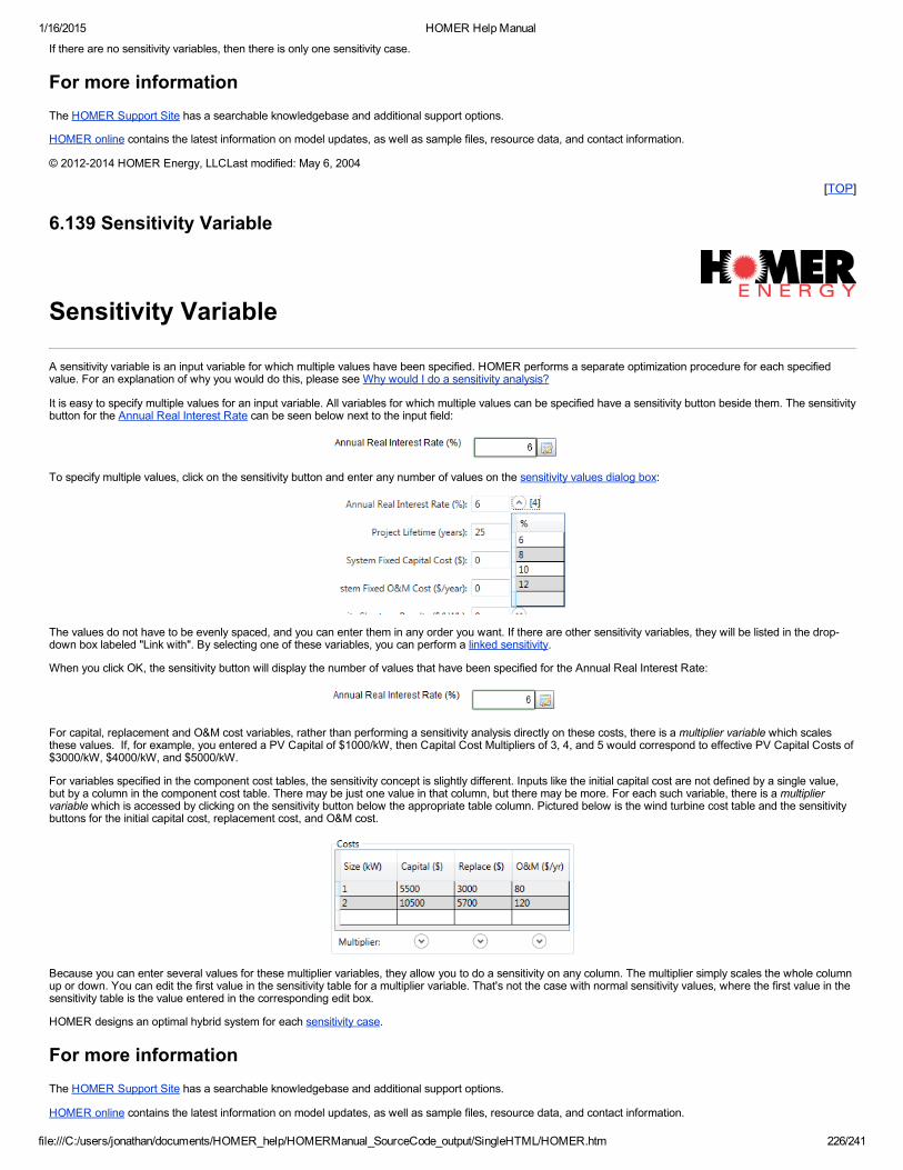
1/16/2015 HOMER Help Manual
file:///C:/users/jonathan/documents/HOMER_help/HOMERManual_SourceCode_output/SingleHTML/HOMER.htm 226/241
If there are no sensitivity variables, then there is only one sensitivity case.
For more informationThe HOMER Support Site has a searchable knowledgebase and additional support options.
HOMER online contains the latest information on model updates, as well as sample files, resource data, and contact information.
© 20122014 HOMER Energy, LLCLast modified: May 6, 2004
[TOP]
6.139 Sensitivity Variable
Sensitivity Variable
A sensitivity variable is an input variable for which multiple values have been specified. HOMER performs a separate optimization procedure for each specifiedvalue. For an explanation of why you would do this, please see Why would I do a sensitivity analysis?
It is easy to specify multiple values for an input variable. All variables for which multiple values can be specified have a sensitivity button beside them. The sensitivitybutton for the Annual Real Interest Rate can be seen below next to the input field:
To specify multiple values, click on the sensitivity button and enter any number of values on the sensitivity values dialog box:
The values do not have to be evenly spaced, and you can enter them in any order you want. If there are other sensitivity variables, they will be listed in the dropdown box labeled "Link with". By selecting one of these variables, you can perform a linked sensitivity.
When you click OK, the sensitivity button will display the number of values that have been specified for the Annual Real Interest Rate:
For capital, replacement and O&M cost variables, rather than performing a sensitivity analysis directly on these costs, there is a multiplier variable which scalesthese values. If, for example, you entered a PV Capital of $1000/kW, then Capital Cost Multipliers of 3, 4, and 5 would correspond to effective PV Capital Costs of$3000/kW, $4000/kW, and $5000/kW.
For variables specified in the component cost tables, the sensitivity concept is slightly different. Inputs like the initial capital cost are not defined by a single value,but by a column in the component cost table. There may be just one value in that column, but there may be more. For each such variable, there is a multipliervariable which is accessed by clicking on the sensitivity button below the appropriate table column. Pictured below is the wind turbine cost table and the sensitivitybuttons for the initial capital cost, replacement cost, and O&M cost.
Because you can enter several values for these multiplier variables, they allow you to do a sensitivity on any column. The multiplier simply scales the whole columnup or down. You can edit the first value in the sensitivity table for a multiplier variable. That's not the case with normal sensitivity values, where the first value in thesensitivity table is the value entered in the corresponding edit box.
HOMER designs an optimal hybrid system for each sensitivity case.
For more informationThe HOMER Support Site has a searchable knowledgebase and additional support options.
HOMER online contains the latest information on model updates, as well as sample files, resource data, and contact information.

1/16/2015 HOMER Help Manual
file:///C:/users/jonathan/documents/HOMER_help/HOMERManual_SourceCode_output/SingleHTML/HOMER.htm 227/241
© 20122014 HOMER Energy, LLCLast modified: May 6, 2004
[TOP]
6.140 Setpoint State of Charge
Setpoint State of Charge
The setpoint state of charge is a parameter that can be applied to the cycle charging strategy. If a setpoint state of charge is applied, once the system starts tocharge the battery bank it will not stop until the battery bank reaches the setpoint state of charge.
The setpoint state of charge tends to reduce the amount of time the battery bank spends at a low state of charge. It also tends to reduce the number of generatorstarts and the number of battery chargedischarge cycles that occur thoughout the year.
The setpoint state of charge appears on the System Control Inputs window.
See also
Cycle charging strategy
For more informationThe HOMER Support Site has a searchable knowledgebase and additional support options.
HOMER online contains the latest information on model updates, as well as sample files, resource data, and contact information.
© 20122014 HOMER Energy, LLCLast modified: Sept 28, 2012
[TOP]
6.141 Simulation Time Step
Simulation Time Step
The default simulation time step in HOMER is 1 hour (60 minutes).
HOMER Pro can simulate system operation with any time step from as long as several hours to as short as one minute. You specify the simulation time step on theSystem Control Inputs tab.
The shorter the time step, the more time steps HOMER must simulate to cover one year, so the longer each simulation takes.
The simulation time step does not have to match the time step of any time series data you may have imported. For example, if you import 10minute wind data and60minute load data, and you simulate on a 10minute time step, HOMER will divide each 60minute load value into six identical 10minute values. If you simulateon a 60minute time step, HOMER will aggregate six 10minute wind speed values together into a single 60minute value for each time step. Or you could chooseto simulate using a 30minute time step, in which case it would aggregate the wind values and disaggregate the load values.
For more informationThe HOMER Support Site has a searchable knowledgebase and additional support options.
HOMER online contains the latest information on model updates, as well as sample files, resource data, and contact information.
© 20122014 HOMER Energy, LLCLast modified: January 22, 2010
[TOP]
6.142 Sinking Fund Factor
Sinking Fund Factor

1/16/2015 HOMER Help Manual
file:///C:/users/jonathan/documents/HOMER_help/HOMERManual_SourceCode_output/SingleHTML/HOMER.htm 228/241
The sinking fund factor is a ratio used to calculate the future value of a series of equal annual cash flows. The equation for the sinking fund factor is:
where:i = real interest rateN = number of years
Example: for i = 7% and N = 5 years, the sinking fund factor is equal to 0.1739. Therefore, five annual payments of $173.90 earning 7% interest would be worth$1000.00 at the end of the fifth year.
See also
Capital recovery factor
For more informationThe HOMER Support Site has a searchable knowledgebase and additional support options.
HOMER online contains the latest information on model updates, as well as sample files, resource data, and contact information.
© 20122014 HOMER Energy, LLCLast modified: May 6, 2004
[TOP]
6.143 SO2 Emissions Penalty (PRO)
SO2 Emissions Penalty
Type: Input VariableUnits: $/tSymbol: cSO2
Use the SO2 emissions penalty to penalize systems for their production of sulfur dioxide. HOMER uses this input value when calculating the Other O&M cost.
For more informationThe HOMER Support Site has a searchable knowledgebase and additional support options.
HOMER online contains the latest information on model updates, as well as sample files, resource data, and contact information.
© 20122014 HOMER Energy, LLCLast modified: Sept 28, 2012
[TOP]
6.144 Solar Absorptance
Solar Absorptance
The solar absorptance of a surface is the fraction of the sun's radiation that the surface absorbs.
The solar absorptance is a factor in the calculation of the PV array temperature. But it is a relatively unimportant one, so rather than making you enter it, HOMERuses the assumption suggested by Duffie and Beckman (1991) that the product of the solar absorptance and the solar transmittance is 0.9 or 90%.
See also
Solar transmittance
How HOMER calculates the PV cell temperature
For more information
1/16/2015 HOMER Help Manual
file:///C:/users/jonathan/documents/HOMER_help/HOMERManual_SourceCode_output/SingleHTML/HOMER.htm 229/241
The HOMER Support Site has a searchable knowledgebase and additional support options.
HOMER online contains the latest information on model updates, as well as sample files, resource data, and contact information.
© 20122014 HOMER Energy, LLCLast modified: November 8, 2007
[TOP]
6.145 Solar Transmittance
Solar Transmittance
The solar transmittance of a surface is the fraction of the sun's radiation that are transmitted through the surface.
The solar transmittance is a factor in the calculation of the PV array temperature. But it is a relatively unimportant one, so rather than making you enter it, HOMERuses the assumption suggested by Duffie and Beckman (1991) that the product of the solar absorptance and the solar transmittance is 0.9 or 90%.
See also
Solar absorptance
How HOMER calculates the PV cell temperature
For more informationThe HOMER Support Site has a searchable knowledgebase and additional support options.
HOMER online contains the latest information on model updates, as well as sample files, resource data, and contact information.
© 20122014 HOMER Energy, LLCLast modified: Sept 28, 2012
[TOP]
6.146 Specific Fuel Consumption
Specific Fuel Consumption
Type: Output VariableUnits: L/kWh, m3/kWh, or kg/kWh, depending on the units of the fuelSymbol: Fspec
The specific fuel consumption is the average amount of fuel consumed by the generator per kWh of electricity it generates. HOMER calculates the specific fuelconsumption using the following equation:
where:Ftot = total annual generator fuel consumption [L/yr, m3/yr, or kg/yr]Egen = total annual electrical production of the generator [kWh/yr]
For more informationThe HOMER Support Site has a searchable knowledgebase and additional support options.
HOMER online contains the latest information on model updates, as well as sample files, resource data, and contact information.
© 20122014 HOMER Energy, LLCLast modified: Sept 28, 2012
[TOP]
6.147 Standard Test Conditions

1/16/2015 HOMER Help Manual
file:///C:/users/jonathan/documents/HOMER_help/HOMERManual_SourceCode_output/SingleHTML/HOMER.htm 230/241
Standard Test Conditions
PV manufacturers rate the power output of their PV modules at standard test conditions (STC), meaning a radiation of 1 kW/m2, a cell temperature of 25°C, andno wind. Standard test conditions do not reflect typical operating conditions, since fullsun cell temperatures tend to be much higher than 25°C.
See also
How HOMER calculates the PV cell temperature
For more informationThe HOMER Support Site has a searchable knowledgebase and additional support options.
HOMER online contains the latest information on model updates, as well as sample files, resource data, and contact information.
© 20122014 HOMER Energy, LLCLast modified: November 12, 2007
[TOP]
6.148 Suggested Lifetime Throughput
Suggested Lifetime Throughput
HOMER calculates a suggested value of lifetime throughput for a battery based on the information entered in the lifetime curve. The suggested value is equal to theaverage value of the lifetime throughput values that fall within the allowable range of depth of discharge. (This allowable range is determined by the minimum stateof charge if the minimum state of charge is 40%, then the battery will only experience depths of discharge between 0% and 60%.) You can accept the suggestedvalue or modify it according to your judgement.
See also
Battery lifetime throughput
Create New Battery window
For more informationThe HOMER Support Site has a searchable knowledgebase and additional support options.
HOMER online contains the latest information on model updates, as well as sample files, resource data, and contact information.
© 20122014 HOMER Energy, LLCLast modified: Sept 28, 2012
[TOP]
6.149 System
System
In HOMER documentation, the word system refers to the combinations of technologies and components of a power generation system. The terms system type andsystem configuration have different meanings that are described below.
System typeA system type is a combination of technologies. For example, wind/diesel/battery describes a system type that includes wind turbines, diesel generators, andbatteries.
System configurationA system configuration is a combination of particular numbers and sizes of components. For example, a system with a generic 10 kW wind turbine, 15 kW diesel

1/16/2015 HOMER Help Manual
file:///C:/users/jonathan/documents/HOMER_help/HOMERManual_SourceCode_output/SingleHTML/HOMER.htm 231/241
generator, 32 batteries and a 6 kW inverter describes a configuration of the wind/diesel/battery system type. The same system type with 48 batteries is a differentsystem configuration.
HOMER simulates system configurations. As it searches for the optimal system type, HOMER typically evaluates hundreds or thousands of system configurations.HOMER displays a list of system configurations in the overall optimization results table, and the most cost effective configuration of each system type in thecategorized optimization results table.
A system configuration can also be defined by dispatch strategy. For example, a system consisting of a generic 10 kW wind turbine, 15 kW diesel, 32 batteries, andan inverter could have two configurations: one with a load following dispatch strategy, and another with a cycle charging dispatch strategy.
For more informationThe HOMER Support Site has a searchable knowledgebase and additional support options.
HOMER online contains the latest information on model updates, as well as sample files, resource data, and contact information.
© 20122014 HOMER Energy, LLCLast modified: May 6, 2004
[TOP]
6.150 System Fixed Capital Cost
System Fixed Capital Cost
Type: Input VariableUnits: $Symbol: Ccap,fixed
The system fixed capital cost is the capital cost that occurs at the start of the project regardless of the size or architecture of the power system.
The system fixed capital cost appears in the Cash Flow Details Table as 'other capital cost'. It adds to the total initial capital cost of the system, and therefore to thetotal net present cost. But since it affects the NPC of all system configurations in the search space by the same amount, it has no effect on the system rankings.
See also
System fixed O&M cost
Cash Flow Details table
Total net present cost
For more informationThe HOMER Support Site has a searchable knowledgebase and additional support options.
HOMER online contains the latest information on model updates, as well as sample files, resource data, and contact information.
© 20122014 HOMER Energy, LLCLast modified: Sept 28, 2012
[TOP]
6.151 System Fixed Operations and Maintenace (O&M) Cost
System Fixed O&M Cost
Type: Input VariableUnits: $/yrSymbol: Com,fixed
The system fixed operation and maintenance (O&M) cost is the recurring annual cost that occurs regardless of the size or architecture of the power system.
The system fixed O&M cost appears in the Cash Flow Details Table as 'other O&M cost'. It affects the total net present cost of each system configuration equally,so it has no effect on the system rankings.
See also

1/16/2015 HOMER Help Manual
file:///C:/users/jonathan/documents/HOMER_help/HOMERManual_SourceCode_output/SingleHTML/HOMER.htm 232/241
System fixed capital cost
Cash Flow Details table
Total net present cost
For more informationThe HOMER Support Site has a searchable knowledgebase and additional support options.
HOMER online contains the latest information on model updates, as well as sample files, resource data, and contact information.
© 20122014 HOMER Energy, LLCLast modified: Sept 28, 2012
[TOP]
6.152 System Roundtrip Efficiency
System Roundtrip Efficiency
Type: Intermediate VariableUnits: noneSymbol: h
The system roundtrip efficiency is the overall efficiency of the system in converting AC energy to DC, putting that energy into storage in the battery bank, removingit from the battery bank, and converting it back to AC. HOMER calculates the system roundtrip efficiency using the following equation:
h = hinv hrt hrect
where:hinv = inverter efficiency
hrt = battery roundtrip efficiencyhrect = rectifier efficiency
For more informationThe HOMER Support Site has a searchable knowledgebase and additional support options.
HOMER online contains the latest information on model updates, as well as sample files, resource data, and contact information.
© 20122014 HOMER Energy, LLCLast modified: May 6, 2004
[TOP]
6.153 Thermal Load Served (PRO)
Thermal Load Served
Type: Output VariableUnits: kWh/yrSymbol: Hserved
The thermal load served is the total amount of thermal energy that went towards serving the thermal load during the year.
For more informationThe HOMER Support Site has a searchable knowledgebase and additional support options.
HOMER online contains the latest information on model updates, as well as sample files, resource data, and contact information.

1/16/2015 HOMER Help Manual
file:///C:/users/jonathan/documents/HOMER_help/HOMERManual_SourceCode_output/SingleHTML/HOMER.htm 233/241
© 20122014 HOMER Energy, LLCLast modified: Sept 28, 2012
[TOP]
6.154 Total Annualized Cost
Total Annualized Cost
Type: Output VariableUnits: $/yearSymbol: Cann,tot
The total annualized cost is the annualized value of the total net present cost. HOMER calculates the total annualized cost using the following equation:
where:CNPC,tot = the total net present cost [$]i = the annual real interest rate [%]Rproj = the project lifetime [yr]CRF() = a function returning the capital recovery factor
HOMER uses the total annualized cost to calculate the levelized cost of energy.
See also
Annualized cost definition
Total net present cost
Levelized cost of energy
Cash Flow Details table
For more informationThe HOMER Support Site has a searchable knowledgebase and additional support options.
HOMER online contains the latest information on model updates, as well as sample files, resource data, and contact information.
© 20122014 HOMER Energy, LLCLast modified: Sept 28, 2012
[TOP]
6.155 Total Capacity Shortage
Total Capacity Shortage
Type: Output VariableUnits: kWh/yrSymbol: Ecs
The total capacity shortage (or annual capacity shortage) is the total amount of capacity shortage that occurs throughout the year. At the end of the year, this valueis used to calculate the capacity shortage fraction.
Note that if each of the four operating reserve inputs (specified on the Constraints window) are set to zero, the total capacity shortage will be equal to the totalunmet load.
See also

1/16/2015 HOMER Help Manual
file:///C:/users/jonathan/documents/HOMER_help/HOMERManual_SourceCode_output/SingleHTML/HOMER.htm 234/241
Required operating reserve
Maximum annual capacity shortage
Capacity shortage fraction
Total unmet load
For more informationThe HOMER Support Site has a searchable knowledgebase and additional support options.
HOMER online contains the latest information on model updates, as well as sample files, resource data, and contact information.
© 20122014 HOMER Energy, LLCLast modified: Sept 28, 2012
[TOP]
6.156 Total Electrical Load Served
Total Electrical Load Served
Type: Output VariableUnits: kWh/yrSymbol: Eserved
The total electrical load served is the total amount of energy that went towards serving the primary and deferrable loads during the year, plus the amount of energysold to the grid. HOMER calculates the total electrical load served using the following equation:
where:Eserved,primAC = AC primary load served [kWh/yr]Eserved,primDC = DC primary load served [kWh/yr]Eserved,def = deferrable load served [kWh/yr]Egrid,sales = energy sold to the grid [kWh/yr]
HOMER uses this value to calculate the renewable fraction and the levelized cost of energy.
See also
Renewable fraction
Levelized cost of energy
Total thermal load served
For more informationThe HOMER Support Site has a searchable knowledgebase and additional support options.
HOMER online contains the latest information on model updates, as well as sample files, resource data, and contact information.
© 20122014 HOMER Energy, LLCLast modified: Sept 28, 2012
[TOP]
6.157 Total Electrical Production
Total Electrical Production

1/16/2015 HOMER Help Manual
file:///C:/users/jonathan/documents/HOMER_help/HOMERManual_SourceCode_output/SingleHTML/HOMER.htm 235/241
Type: Output VariableUnits: kWh/yrSymbol: Eprod
The total electrical production is the total amount of electrical energy produced by the power system in one year. It is the sum of the electrical energy produced byall components of the system.
See also
Total thermal production
Renewable electrical production
For more informationThe HOMER Support Site has a searchable knowledgebase and additional support options.
HOMER online contains the latest information on model updates, as well as sample files, resource data, and contact information.
© 20122014 HOMER Energy, LLCLast modified: Sept 28, 2012
[TOP]
6.158 Total Thermal Production (PRO)
Total Thermal Production
Type: Output VariableUnits: kWh/yrSymbol: Hprod
The total thermal production is the total amount of thermal energy produced by the power system in one year. It is the sum of the thermal energy produced by allcomponents of the system.
See also
Total electrical production
Renewable thermal production
For more informationThe HOMER Support Site has a searchable knowledgebase and additional support options.
HOMER online contains the latest information on model updates, as well as sample files, resource data, and contact information.
© 20122014 HOMER Energy, LLCLast modified: Sept 28, 2012
[TOP]
6.159 Total Excess Electricity
Total Excess Electricity
Type: Output VariableUnits: kWh/yrSymbol: Eexcess
The total excess electricity is the total amount of excess electricity that occurs throughout the year.
See also

1/16/2015 HOMER Help Manual
file:///C:/users/jonathan/documents/HOMER_help/HOMERManual_SourceCode_output/SingleHTML/HOMER.htm 236/241
Excess electricity fraction
For more informationThe HOMER Support Site has a searchable knowledgebase and additional support options.
HOMER online contains the latest information on model updates, as well as sample files, resource data, and contact information.
© 20122014 HOMER Energy, LLCLast modified: Sept 28, 2012
[TOP]
6.160 Total Fuel Cost
Total Fuel Cost
Type: Output Variable
Units: $/yrSymbol: Cfuel,tot
The total fuel cost is the sum of the fuel costs of each generator and the boiler.
For more informationThe HOMER Support Site has a searchable knowledgebase and additional support options.
HOMER online contains the latest information on model updates, as well as sample files, resource data, and contact information.
© 20122014 HOMER Energy, LLCLast modified: Sept 28, 2012
[TOP]
6.161 Total Net Present Cost
Total Net Present Cost
Type: Output VariableUnits: $Symbol: CNPC
The total net present cost (NPC) of a system is the present value of all the costs that it incurs over its lifetime, minus the present value of all the revenue that itearns over its lifetime. Costs include capital costs, replacement costs, O&M costs, fuel costs, emissions penalties, and the costs of buying power from the grid.Revenues include salvage value and grid sales revenue.
HOMER calculates the total NPC by summing up the total discounted cash flows in each year of the project lifetime. The total NPC appears in the bottomright cellof the Cash Flow Details Table.
Tip: Look at the Cash Flow Details Table to see a precise itemization of the cash flows that contribute to the total net present cost.
The total NPC is HOMER's main economic output, the value by which it ranks all system configurations in the optimization results, and the basis from which itcalculates the total annualized cost and the levelized cost of energy.
See also
Cash Flow Details table
Net present cost definition
Total annualized cost
Levelized cost of energy
Why does HOMER rank systems by total NPC?
1/16/2015 HOMER Help Manual
file:///C:/users/jonathan/documents/HOMER_help/HOMERManual_SourceCode_output/SingleHTML/HOMER.htm 237/241
For more informationThe HOMER Support Site has a searchable knowledgebase and additional support options.
HOMER online contains the latest information on model updates, as well as sample files, resource data, and contact information.
© 20122014 HOMER Energy, LLCLast modified: Sept 28, 2012
[TOP]
6.162 Total Unmet Load
Total Unmet Load
Type: Output VariableUnits: kWh/yrSymbol: Eunmet
The total unmet load is the total amount of unmet load that occurs throughout the year.
For more informationThe HOMER Support Site has a searchable knowledgebase and additional support options.
HOMER online contains the latest information on model updates, as well as sample files, resource data, and contact information.
© 20122014 HOMER Energy, LLCLast modified: Sept 28, 2012
[TOP]
6.163 Unmet Load
Unmet Load
Unmet load is electrical load that the power system is unable to serve. It occurs when the electrical demand exceeds the supply. For each system, HOMERcalculates the total unmet load that occurs over the year, as well as the unmet load fraction. By default, HOMER considers infeasible any system that experiencesunmet load, but you can change that by entering a nonzero value for the maximum annual capacity shortage.
See also
Capacity shortage
Unmet load fraction
For more informationThe HOMER Support Site has a searchable knowledgebase and additional support options.
HOMER online contains the latest information on model updates, as well as sample files, resource data, and contact information.
© 20122014 HOMER Energy, LLCLast modified: May 6, 2004
[TOP]
6.164 Unmet Load Fraction
Unmet Load Fraction

1/16/2015 HOMER Help Manual
file:///C:/users/jonathan/documents/HOMER_help/HOMERManual_SourceCode_output/SingleHTML/HOMER.htm 238/241
Type: Output VariableUnits: noneSymbol: funmet
The unmet load fraction is the proportion of the total annual electrical load that went unserved because of insufficient generation. The equation for the unmet loadfraction is given below:
where:Eunmet = total unmet load [kWh/yr]Edemand = total annual electrical demand (primary plus deferrable) [kWh/yr]
For more informationThe HOMER Support Site has a searchable knowledgebase and additional support options.
HOMER online contains the latest information on model updates, as well as sample files, resource data, and contact information.
© 20122014 HOMER Energy, LLCLast modified: Sept 28, 2012
[TOP]
6.165 Weibull Distribution
The Weibull Distribution
The twoparameter Weibull distribution is often used to characterize wind regimes because it has been found to provide a good fit with measured wind data. Theprobability density function is given by the following equation:
where:v is the wind speed [m/s]k is the Weibull shape factor [unitless]c is the Weibull scale parameter [m/s]
The cumulative distribution function is given by the following equation:
The following equation relates the two Weibull parameters and the average wind speed:
where:G is the gamma function
One can describe a Weibull distribution by an average wind speed and a Weibull k value. The graph below shows five Weibull distributions, all with the sameaverage wind speed of 6 m/s, but each with a different Weibull k value. As the graph shows, lower k values correspond to broader distributions.
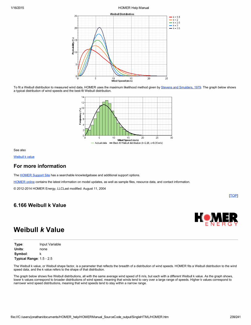
1/16/2015 HOMER Help Manual
file:///C:/users/jonathan/documents/HOMER_help/HOMERManual_SourceCode_output/SingleHTML/HOMER.htm 239/241
To fit a Weibull distribution to measured wind data, HOMER uses the maximum likelihood method given by Stevens and Smulders, 1979. The graph below showsa typical distribution of wind speeds and the bestfit Weibull distribution.
See also
Weibull k value
For more informationThe HOMER Support Site has a searchable knowledgebase and additional support options.
HOMER online contains the latest information on model updates, as well as sample files, resource data, and contact information.
© 20122014 HOMER Energy, LLCLast modified: August 11, 2004
[TOP]
6.166 Weibull k Value
Weibull k Value
Type: Input VariableUnits: noneSymbol: kTypical Range: 1.5 2.5
The Weibull k value, or Weibull shape factor, is a parameter that reflects the breadth of a distribution of wind speeds. HOMER fits a Weibull distribution to the windspeed data, and the k value refers to the shape of that distribution.
The graph below shows five Weibull distributions, all with the same average wind speed of 6 m/s, but each with a different Weibull k value. As the graph shows,lower k values correspond to broader distributions of wind speed, meaning that winds tend to vary over a large range of speeds. Higher k values correspond tonarrower wind speed distributions, meaning that wind speeds tend to stay within a narrow range.

1/16/2015 HOMER Help Manual
file:///C:/users/jonathan/documents/HOMER_help/HOMERManual_SourceCode_output/SingleHTML/HOMER.htm 240/241
Lower k values correspond to broader wind speed distributions. So a very gusty location may have a Weibull k value as low as 1.5 or so, whereas a locationcharacterized by very steady winds (like tropical trade wind environments) may have a k value as high as 3 or 4. When you synthesize wind speed data, HOMERuses a default Weibull k value of 2, which is typical of many wind regimes.
When fitting a Weibull distribution to measured wind data, HOMER uses the maximum likelihood method given by Stevens and Smulders, 1979.
To help HOMER users estimate Weibull k values in the absence of measured data, we calculated the bestfit Weibull k value for each of the 239 weather stationsin the TMY2 data set. The histogram below shows the resulting distribution of Weibull k values. The measured values themselves appear in the table of measuredwind parameters.
In the TMY2 data set, we observed a correlation between the Weibull k value and the average wind speed, with higher annual average wind speeds tending tocorrespond to lower Weibull k values. The graph below displays this correlation:
See also
Weibull distribution
Autocorrelation factor
Diurnal pattern strength
Hour of peak wind speed
TMY2 wind parameters

1/16/2015 HOMER Help Manual
file:///C:/users/jonathan/documents/HOMER_help/HOMERManual_SourceCode_output/SingleHTML/HOMER.htm 241/241
For more informationThe HOMER Support Site has a searchable knowledgebase and additional support options.
HOMER online contains the latest information on model updates, as well as sample files, resource data, and contact information.
© 2012 HOMER Energy, LLCLast modified: Sept 28, 2012
[TOP]
6.167 Wind Turbine Hub Height
Wind Turbine Hub Height
Type: Input VariableUnits: mSymbol: zhub
The wind turbine hub height is the height above ground at which the rotor sits. Hub heights typically range between 25m (for smaller wind turbines, 50 kW or less)and 100m (for large, multimegawatt wind turbines). Wind speeds tend to increase with height above ground, so if the hub turbine is not the same as theanemometer height, HOMER adjusts the wind speed data accordingly.
For details on how HOMER calculates the wind speed at the hub height of the wind turbine, see Wind shear inputs.
See also:
Wind shear inputs
Anemometer height
For more informationThe HOMER Support Site has a searchable knowledgebase and additional support options.
HOMER online contains the latest information on model updates, as well as sample files, resource data, and contact information.
© 20122014 HOMER Energy, LLCLast modified: Sept 28, 2012
[TOP]