homeowners insurance ratemaking

HOMEOWNERS INSURANCE RATEMAKING

MICHAEL A. WALTERS

The approach taken in this paper is a little different from some other ratemaking papers in that no specific historical development was attempted. The only historical background felt to be needed was the “invention” of the homeowners policy in the 1950’s and the introduction of a more detailed statistical plan in the 1960’s. Because the homeowners policy is not much beyond its infancy, or at most adolescence, it is not surprising to find changes in ratemaking techniques occurring more frequently for this line of insurance. These changes are generally inspired by new insights into the nature of the coverage or by greater awareness of the statistical plan capabilities.

Because of these inevitable changes in techniques, and since ratemaking papers in the CAS Proceedings are not updated annually, the procedures described in this paper may not be “current” for very long. However, they can provide insight for other lines of insurance with similar problems, in addition to bringing the record up-to-date at least as of 1974. The main purpose, therefore, was to deal with some of the important concepts in Home- owners ratemaking and to illustrate some appropriate procedures consistent with basic ratemaking principles and made possible by the available statistical data.

The contents are not sufficient for a complete “Cookbook”. and in order to keep the length of the paper manageable. presume a basic knowledge of policy forms, coverages, and statistical plans. The scope of the paper consists of:

1)

2)

3)

4)

5)

6)

General ratemaking perspective;

Statewide ratemaking for the basic policy forms (HO- I. 2, 3 81 5);

Territory ratemaking for the same forms;

Tenants Form (HO-4) ratemaking;

Summary and conclusions;

Appendices including some classification treatment of Policy Form and Amount of Insurance, as well as more detailed devclop- ments not appropriate for the body of the paper.

16 HOMEOWNERS INSLRANCE RATEb,AK,NC

In addition to describing the procedures within each topic, some justifi- cation and perspective will also be given, along with any alternative methods that come to mind. Although the procedures are basically taken from ;L rating bureau standpoint (i.c. Insurance Services Office). some application can be made to individual company raternuking.

SOME PERSPECTIVES ON RAT EMAKISG

Since one of the most difficult elements of the “scientific method” i4 the proof or verification of the hypothesis involved, perhaps insurance ratemaking should be viewed ;1s more of an art than ;I science because no one can scientifically guarantee the future.With this in mind, insurance ratemaking could be defined as the art of projecting scientifically measured past experience into valid (but not absoluteI> certain) conclusion5 about future insurance experience.

Usually one of three situation?, or stages confront5 the ratemaker in his attempt to project the future for a line of insurance. The first occurs when no data is available, or essentially when ;I new product is being formed; the next stage occurs when experience exists. with no expected changes in the nature of the product; and lastly when experience exists but modifications in coverage are expected to take place. Given the basic tenet in the art of ratemaking

that “history will repeat itself’, Stage Two is ohviou\ly the easicht environment in which to make rates.

Stage One No Data

Stage One is a most difficult time for ratemakers, especially when 3 product like Homeowners insurance comes along. with the packaging of many heretofore separate coverages on a mandator) ba\ir, into one policy. It may have been true that the contractual coverages looked similar to the monoline policies for fire. windstorm, theft, other physical damage. and personal liability; but no one could predict with accuracy the behavior of insureds with all those coverages together. Not only U;IS “adverse selection” eliminated by mandating all these coverages. but amounts of insurance were also preordained for contents (both on and away from premises) once the value of insurance on the dwelling building w;i\ determined. This eliminated or reduced substantially the problems of underinsurance.

The result of all this was a policy form with lower pure premiums (loss cost per unit of exposure) for each of the coverages involved than on a monoline level where insured\ map select only those coverage5 the) think arc ncces-

HOMEOWNERS INSURANCE RATEMAKING 17

sary, choosing to self-insure those hazards with much lower expected losses. The spread of loss achieved from this packaging of coverages on a mandatory basis gives the policyholder more coverage at a much lower total pure premium than obtained from buying the monoline policies separately, plus the advantage of the expense savings in a package policy. In this regard, no more successful package policy has existed before, nor is likely to be devised again, because of the nature of the hazards covered and the type of market involved.

The ratemaking for this first phase necessarily contains a lot of judgment, with the selection of package discounts from the monoline policy costs being based more on theory and hope than on empirical data. The rapid development of actual experience under the new product depends, of course, on its success in the marketplace. Ideally, the use of actual experience rapidly substitutes for the initial estimates based on theory and judgment.

Stage Tccro-Actual Experience

For Homeowners insurance, Stage Two built up rapidly with not too many of the transitional problems of having both monoline and package policies marketed simultaneously to the same types of customers. Consequently, the actual experience collected under Homeowners insurance could be used directly and more quickly in appropriate projections of the future experience for purchasers of this coverage.

Of course, ratemaking is not as simple as “history repeating itself’. Even for 21 line of insurance remaining fairly stable as regards type of coverage, there is more to predicting the future than knowing precisely what hap- pened in the past.

Certain modifications are needed to put past experience on current conditions. Premium levels may have changed such that today’s manual rates are different from those in effect during the past experience period. Loss patterns may be changing such that a past year’s value is but one observation in a changing sequence of pure premiums due to inflation, increased affluence, varying accident frequencies, and changes in claim consciousness. Further- more, the observed experience in the past may have been a non-typical value owing to random fluctuations inherent in the data or to unusual events with a cyclical frequency extending beyond one or even ten years in cycle.

These phenomena, of current level adjustments, trend. credibility. and catastrophe, are present to some extent in every line of insurance and will be discussed in more detail in the procedures for Homeowners insurance ratemaking.

I8 HOMEOWNERS INSURANCE RATEMAKING

Stage Three- Changes in Coverages Marked changes in coverage or conditions cause additional difftculties

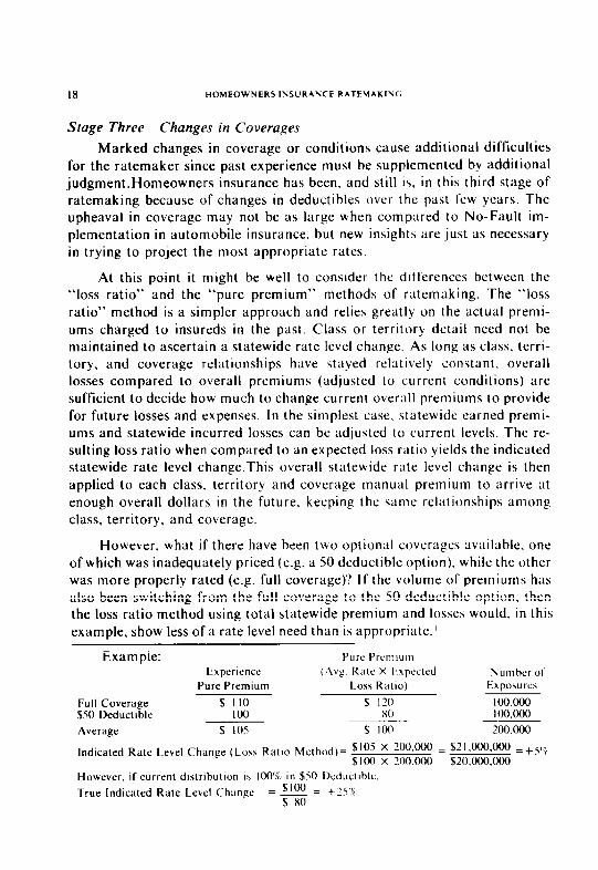
for the ratemaker since past experience must be supplemented by additional judgment.Homeowners insurance has been. and still is. in this third stage of ratemaking because of changes in deductibles over the past few years. The upheaval in coverage may not be as large when compared to No-Fault implementation in automobile insurance. but new insights are just as necessary in trying to project the most appropriate rates.

At this point it might be well to consider the differences between the “loss ratio” and the “pure premium” methods of ratemaking. The “loss ratio” method is a simpler approach and relies greatly on the actual premiums charged to insureds in the past. Class or territory detail need not be maintained to ascertain a statewide rate level change. As long as class. territory, and coverage relationships have stayed relatively constant, overall losses compared to overall premiums (adjusted to current conditions) are sufficient to decide how much to change current overall premiums to provide for future losses and expenses. In the simplest case, statewide earned premiums and statewide incurred losses can be adjusted to current levels. The resulting loss ratio when compared to an expected loss ratio yields the indicated statewide rate level change.This overall statewide rate level change is then applied to each class, territory and coverage manual premium to arrive at enough overall dollars in the future, keeping the same relationships among class, territory, and coverage.

However. what if there have been t\ro optional coverages available, one of which was inadequately priced (e.g. a 50 deductible option), while the other was more properly rated (e.g. full coverage)? If the volume of premiums has also been switching from the full coverage to the 50 deductible option, then the loss ratio method using total statewide premium and losses would, in this example, show less of a rate level need than is appropriate.’

Example:

Full Coverage $50 Deductible

Average

Experience Pure Premium

$ II0 IO0

$ 10s

Pure Prcmtum ( Avg Rate X k.xpccted

Loss Ratio)

$ 120 x0

$ loo

Number ol Exposures

100.000 ioO.000

200.000

Indicated Rate Level Change (Loss Ratlo Method)= $ I05 x 200,000 = $2 I ,OOO.Ot.Kl = + 5’~(, .slOO x 3~0.000 $20.ooo.ooo

However. if current distribution is 100’S in $50 Deductible.

True Indicated Rate Level Change = $100 = f’5’P, $ x0


The “pure premium” approach, on the other hand, would have the abili- ty to identify the average loss per policy for each of the two coverages separately. It has the advantage of being independent of the actual premiums that were charged in the past and of the relative adequacy by class, territory or coverage. Taking the set of exposures in the past that produced the experience pure premiums, the current manual rates can be used to hypothetically re-rate those exposures as a test of the adequacy of today’s rates. In addition, if only one coverage is being offered now, then the exposures can be extended at that particular set of rates, and the pure premiums can be modified accordingly.

Expressed more simply, the “pure premium” method is more concerned with rating a particular coverage properly, regardless of what the average insured may have paid or is paying today. After the coverage is rated, then an effort is made to see what the change is for the average insured to arrive at the new rate. On the other hand, the “loss ratio” method first determines an indicated change in rates. The difficulty with that method is then to find out whether some of the change has already been accomplished by recent switches in coverage or class.

STATEWIDE RATE LEVEL FOR BASIC HOMEOWNERS POLICY FORMS

Lest this paper dwell too long in a theoretical vein, it would be worth- while to look at an example of a statewide rate level-review. However, so that a concrete illustration won’t bore the reader with simplicity, a further com- plication is introduced into the theory. Let us say that two optional coverages have existed in a state for some time: full coverage and a $50 disappearing deductible2 on Section I (non-Liability) perils, with only the deductible premiums now being displayed in the manual. Suppose the intention is to withdraw those two options and only offer a third coverage in the future- namely, a $100 flat deductible on Section I perils. The idea is to test the adequacy of the current manual premiums (although they are for $50 deductible coverage) as being possibly appropriate for the new $100 deductible coverage. In case any changes are indicated, the resulting change in premiums might be a convenient way of calculating the new rate for the new coverage, but it would be insufficient to describe the entire transaction. The true rate level change would be the combination of the premium level change to the

2 $50 deductible “disappears” at $500 via formula: Deductible amount equals $50 less I I% of loss amount above $50 up to $500.

20 HOMEOWNERS INSURANCE RATEMAKINC;

present mix of deductible options and the change in coverage from the present options to a $100 Flat deductible.

Adjusted Premiums

For many lines of insurance. the traditional way of adjusting premiums for ratemaking purposes was to start with the actual written premiums. In addition to being earned into a particular calendar period, they would also be adjusted to current level by means of “on-level” factor based upon price changes since the policies were originally written. This usually entails making assumptions as to when the policies were actually written (with the average policy customarily assumed to be written .luly I, for example). Of course, any varying changes by class, territory, or coverage would compound the assumptions or calculations necessary to convert past premiums to current levels.

With the advent of computers, data bases, and more sophisticated statistical plans, however, many of those assumptions need not be made in arriving at premiums adjusted to current level. The existonce of exposures in class and territory detail, for example, permits the calculation of premiums at present manual rates by extending each set of exposures by class and territory by the appropriate present manual rates. By accumulating the results over all classes and territories, a statewide total of adjusted premiums is produced without ever having to deal with past collected premiums and making assumptions on subsequent changes.Furthermore. a much better estimate is also produced for each subset of statewide totals, such as by territory or by class, for purposes of reviewing relative adequacy of the rates for those subsets. This method is also superior when experience for many insurance companies is pooled. because of the possibility of non-uniformity hy company of both past rate levels and effective dates of changes in rate levels.

For Homeowners insurance, this method of extending exposures has the further advantage of being able to hypothetically re-rate all insureds at one particular coverage, regardless of what they had originally purchased. For example, if a mixture of full coverage and $50 disappearing deductible policies had been sold in the past, enough information is retained on the statistical record to extend all those policies at the current manual rates for the $50 deductible. The important concept is that adjusted premium\ can represent a past set of insureds evaluated at a particular sot of current rates for a speci- fied coverage. Inherently, this exposure extension technique is a “pure premium” method rather than a “loss ratio” method of ratemaking.

The example given below illustrates the major steps involved in the com-


puter calculation of adjusted premiums from full class and territory detail. The computer scans the records sorted by state, territory, policy form, construction, protection, and amount of insurance. Written exposures in house years are then earned into calendar segments (“earned quarters”) by means of term and inception month. The earned exposures in house-years for a calendar year or fiscal year (consisting of the sum of four appropriate earned quarters) are then multiplied by the corresponding annual premium for a particular coverage (usually the broadest deductible displayed in the manual). The manual premium depends upon the territory, policy form, construction and protection class, as well as the amount of insurance.

COMPUTER DEVELOPMENT OF ADJUSTED PREMIUM

(1) (2) (3) (4) (5) (6) (7) Unilq

($15.000) Polic> Tolal Earned Premium Sire Ad.iuated

Number of For Broadesl Kelativit) Premium Detail Cla\\ Code tlouse Years Deductible Factor (4) x (5) x (5)

SklkY: xtr; TX Territory: 4) YV Policy Form: t-arm I I

CwWruclion: Brick 3 Proteclion: 3 3 Amt. of Inwrance:

$ I0.000 IO 25.0 $49 .X6 $1.052.50

512.000 I2 6.0 WY .90 ‘64.60

$ I5.000 I5 45.0 $49 I .oo 2.2os.00

Additional factors’ are then applied in appropriate detail to account for increased limits of liability, and additional endorsements such as credit card,

Statistical Plan changes cffcctwe January I. lY74 will facilitate the caiculalion of hnsicctrver- ape lowz\ and thcrcforc the elimination or modification of thebe additional factor\. For excample. watercrafl. snwmobllc. and secondary dwelling\ will hc idenlified on wparntc rc- porting records. A new “Type of Los\” code will also permit the suhtraclion ofcxc~‘~s cover- ape Iusws from the tolal in order to mow Ltccuratel) price the “basic” tlomeo\cner~ coveragcs found in ever) policy.

22 HOMEOWNERS INSLRAN(‘E RATE?.,AKINC,

snowmobile, watercraft, etc. The result of all these detail calculations are summarized on u statewide basis and appear in Column (I) of the Statewide Rate Level Exhibit as “Adjusted Premiums”. In Exhibit I the current broadest deductible used as the input premium was assumed to be a $50 disappearing deductible on Section I perils. Consequently, the initial evaluation will be to test those premiums for adequaq in providing $100 Flat deductible coverage in the future.

The base from which adjustments are made consists of accident year incurred losses4 as reported in class detail. This mean\ that as of 3 particular evaluation date. e.g. March 31, 1973. accident year 1972 incurred losses are defined as all losses on accidents occurring during calendar year 1972 which were paid BS of March 31, 1973, or which were unpaid its of then but which had loss reserves set up and reported as of March 3 I, 1973. Loss development factors are obviously needed, as incurred-but-not-reported (I BNR) claims may exist three months after the end of the year, for which no payments have been made nor reserves set up. In addition, the reserves as of March 3 I, I973 are likely to be imprecise (generally to the same extent as I5 month reserves have been in the past) when payments are ultimately traced out.

Loss development factors for Homeowners insurance can be calculated in similar fashion as automobile liability insurance. Gencrallg, for an accident year valued as of I.5 months, they average less than 1.03 on :I countrywide basis, but can vary by state. depending upon the percentage of liability losses. (See Appendix B.)

If changes in deductible are contemplated, as ih the case in Exhibit I. then adjustments should be made to convert the past losses to the new deductible level. In this particular state, the conversion is principally from a $50 disappearing deductible to a $100 flat deductible. However. since full coverage had been offered in the past, the losses under those policies must also be converted to a $100 deductible level.

’ Calendar )ear Incurred iosszs can also bc u\cd. consisting of calendar >car paid lwses plus the increase In reserves over the calendar year period. If’ reserve\ in class detail arc used in this calculation. a factor for the change in IBNK reserves (not included In class detail re-

serves) should be applied to the total. \tncr only the paid IRNK lose\ arc in the total paid

losses. See Charles F. Cook. “Trend and 1.~~ Development i’actor\“. K‘.JS. Vol. L-VI I

(1970) p. 15.


The method of conversion is through loss elimination ratios (LER’s). Since the effect of a deductible will vary according to the distribution by size of loss, LER’s should be calculated for each subset of losses which are likely to have a different size of loss distribution.. Fire losses tend to have a much higher average size of claim than theft losses. (It is more difficult to imagine a total loss by theft than by fire.) Different policy forms are also likely to produce different average sizes of loss.

LER’s are currently developed by cause of loss by policy form. (See Appendix A for method of calculation.) For credibility purposes, countrywide distributions by size of claim are usually utilized separately for each cause of loss and policy form. Once established, these LER’s can be applied to a particular state’s own loss distributions, including territory and class. The result of applying LER’s in full class detail with summarization back to a stalewide level is shown in Column (2) of Exhibit I, as “Losses Adjusted to $100 Flat Deductible.”

Catastrophe Losses

From a statistical plan standpoint, a “serialized loss” is defined as any loss arising from an event designated with a Catastrophe Serial Number. A Catastrophe Serial Number is currently assigned shortly after an event by the Statistical Agent (ISO) if all insured property losses from that event are expected to exceed one million dollars for all lines of insurance in all slates. Generally, Catastrophe Serial Numbers arise from hurricanes and large tor- nadoes, and possibly explosions or large area fire conflagrations. For Home- owners insurance currently, “catastrophe losses” are defined to be the sum of all “serialized losses” in a state for each year.

Conceptually, a catastrophe loss is one which ought not be assigned ex- clusively to the year it occurred because of its unusually large size and infre- quent nature. Large hurricanes do not occur every year, and to penalize insureds with a huge rate level increase the year after such an occurrence is to ignore a fundamental precept that ratemaking is not intended to recoup past losses but rather to predict future experience. By the same token, if no hurricanes or other catastrophes have occurred during the experience period under review (now five years for Homeowners insurance5), it would also be a -- ’ Some states require consideration of “at least five years” experience in reviewing property

insurance rate levels. It remains to be \een whether a long-term catastrophe experience period would be sufficient to satisfy the intent of these regulations. This would enable the basic (non-catastrophe element) experience period to be shortened further to three or even two years of premium and loss experience. provided enough volume existed on B statewide basis for credibility purposes. A two or three year experience period might also require the “nor- malization” of other fluctuating (though not catastrophe) perils by means of some averaging process.

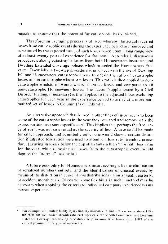
24 HOMEOWNER\ ISSL:KAN( t KA,k\,AKINC,

mistake to assume that the potential for catastrophe has vanished.

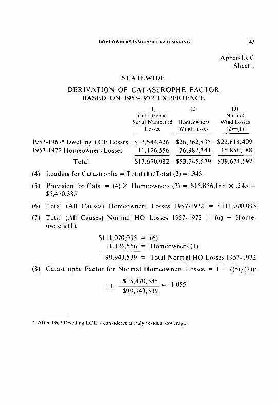
Therefore. an averaging process is utilized uhereby the actual incurred losses from catListrophic events during the experience period are removed and substituted by the expected value of such losses based upon a long range view of at least twenty years of experience for that state. Appendix C discusses a procedure utilizing catastrophe losses from both tlomeouners insurance and Dwelling Extended Coverage policies which preceded the tiomeowners Pro- gram. Essentially. a two-step procedure is involved, \vith the use of Dwelling EC and Homeowners catastrophe losses to obtain the ratio of catastrophe losses to non-catastrophe windstorm losses. This ratio is then applied to non- catastrophe windstorm Homeowners insurance losses and compared to all non-catastrophe Homeowners losses. This factor (supplemented by a Civil Disorder loading. if necessary) is then applied to the ad.justcd losses excluding catastrophes for each year in the experience period to arrive at a more nor- malired set of losses in Column (5) of Exhibit I.

An alternative approach that is used in other lines of insurance is to keep some of the catastrophe losses in the year they occurred and remove only the excess portion over some specific capD. This implies that perhaps the frequency of event was not so unusual as the severity of loss. A case could he made for either approach. and admittedly either one would show a certain distortion if adjusted loss ratios were used to attempt a loss ratio trending procedure. (Leaving in losses below the cap still shous a high “normal” loss ratio for the year. while removing all losses from the catastrophic event, would depress the “normal” loss ratio.)

A future possibility for Homeowner\ insurance might be the elimination of serialired numbers entirely, and the identification of unusual events by means of the distortion in cause of loss distributions on an annual, quarterly. or accident month basis. Of course, some flexibility in such ;I method may be necessary when applying the criteria to individual company experience versus bureau experience.

* For ewmple. automohilc bodily anlurk liabllit) Inwrance c~cludcs SYCCI\ IOSVZS above $10.. 000/$20.000 from ha\ic atewide rate level cxperlencc. \+hile both Commercial and Dwelling

Extended Coverage ratcmakInp procedure keep an amount 111 Iww\ up to IOO”~ of the

earned premlurn in the !car of wcurrcncc


Loss Adjustment Expenses

Countrywide expenses as reported in the Insurance Expense Exhibit by company are broken into various functions: General Expense, Acquisition, Taxes, and Loss Adjustment Expenses. While the first three vary more with total premium volume, loss adjustment expenses are more logically a function of losses. Therefore, for Homeowners insurance, the ratio of loss adjustment expenses incurred to pure losses incurred obtained from the Insurance Expense Exhibit can be applied to the accident year incurred losses on a statewide basis to produce losses including Loss Adjustment Expense as shown in Column (6) of Exhibit I. It currently takes about eleven cents to settle each dollar of a Homeowners claini for the average company.

Trend Factors Observation of past experience may give the appearance of static condi-

tions, while in Fact certain dynamics are at work which influence both the size and frequency of claims. Inflation is perhaps the best known of these influ- ences, and certainly any prediction of future loss experience should include some measurement of past and expected future changes in claim costs due to the increased cost of goods and services which are covered under the policy provisions.

Claim frequencies (within deductible options) can also be changing in Homeowners insurance due to increases in affluence, rising crime rates, and changes in claims consciousness.

Increases in coverage can also be anticipated as inflation causes a rise in the value of residences. Under current procedures, a price exists in the manuals for increased amounts of insurance which reflects both increased coverage and classification differences between houses of different values, (i.e. due to higher affluence, greater theft risk, etc.). The extent to which the classification difference exceeds the coverage difference at higher amounts of insurance represents a potential offset for expected rises in either claim cost or claim frequency.

For Homeowners insurance a simple trend factor can be utilized to track essentially the inflation element in claim costs. As illustrated in Appendix D, a combination of external indices can be used to develop a Composite Con- struction Cost Index by calendar year and quarter. It is a simple matter then to adjust a past year’s losses to current conditions,via “known” changes in these costs, and furthermore to project future changes based upon the latest rates of change. “Current Cost Factors” and “Trend Factors” represent the respective adjustments of past values to the date of the latest published gov-

26 HOMEOWNERS INSURANCE RATEMAKINCi

ernment figures and the adjustment from that point to the average date of occurrence of losses payable under policies written after the proposed effective date of the new rates. (The average occurrence date would thus be one year past the effective date, assuming annual policies written over a period of one year.)

When exposure and loss information is available in Homeowners insurance for a sufficient period of time, it is in order to test whether the other elements of change should be quantified and brought into use. Increasing affluence can cause claim costs to rise faster than inflation, as well as affect- ing frequency and amounts of insurance. Because of changes in deductibles for Homeowners in the past few years, statewide observed claim frequency may not be used by itself. Pure premiums also have this disadvantage unless loss elimination ratios (LER’s) are used to put the experience on a common deductible level. Even with this, random cause of loss fluctuations can mask a true pattern of changes by state. Nevertheless, some combination of statewide and countrywide pure premium by cause of loss offers perhaps the best chance to test the continued propriety of using government indices as trend factors.

In recent years, both inflation and increasing demand for personal residences has accelerated the cost of houses and the need for increased amounts of insurance to protect the owners. As mentioned before, the current policy size relativity factors provide for both increased coverage and differences in classification for the higher amounts of insurance. Abrupt increases in coverage amounts can therefore provide an increase in price without a commensu- rate increase in risk. (If an insured has been underinsured in the past, however, the increase in price is justified on an individual case basis.)

There are various ways of measuring the increase in premium due to this potential excess of price over true coverage. With the current accumulation of “two exposure bases” in Homeowners (number of house years and amount of insurance years), average amount of insurance can be calculated for a period of years. Average premiums at current manual rates can also be determined using the “extension of exposures” technique.

Because fluctuation in average amounts of insurance can occur from year to year due to abrupt lags and pushes in “insurance to value” as well as the influence of new construction, it is better to avoid using the simple observation of loss ratios for trend purposes or the simple fitting of least squares lines to average amounts of insurance in the past.


Whatever the measurement of this phenomenon may be, it is still likely to require a separate treatment of “current cost factors” and “trend” factors. In the illustration for statewide rate level purposes on Exhibit I, Columns (7) and (8) show Current Cost/Amount Factors and a Trend Factor used to put loss ratios on a prospective experience period level. These factors were derived in Appendix D by one method of factoring out the increase in premium due to increasing amounts of insurance. The change in average policy size relativities is calculated and projected on Sheet 3 of Appendix D. Some tempering is needed to reflect the influence of new construction on average policy size changes.

Indicated Premium .4@stment

The weighting of adjusted loss ratios for all years in the review period is more arithmetical than scientific. With greatest weight given to the most recent year for responsiveness, any reasonable set of weights adding up to 100% could really be used. This presumes that any fluctuations due to catastrophic occurrences are identified and removed. On Exhibit I, weights of. IO. .l5, .20. .25, and .30 are used for the five years. Perhaps in the future, some volume criteria could be imposed to allow for reviews with three or even fewer years of Homeowners insurance statewide normal loss experience.

The “Weighted Adjusted Loss Ratio” obtained in Column 8 of Exhibit I represents a projected average portion of the premium dollar that will be needed to cover losses and loss adjustment expenses at a $100 deductible level. It should be recalled in this example that the premium dollar being tested is the current broadest deductible premium displayed in the manuals in this case, the premium heretofore charged for a $50 disappearing deductible.

The Balance Point Loss Ratio of .602 in this example consists of the portion of the premium dollar that is available to pay losses and loss adjustment expenses. Identical in concept to the Expected Loss and Loss Adjust- ment Ratio for automobile insurance ratemaking, it consists of the sum of various appropriate expense ratios plus an allowance for underwriting profit and contingencies. Using the Insurance Expense Exhibit for an expense review of General Administration Expenses and Other Acquisition Costs, and knowing budget requirements for such items as Taxes. Licenses, and Fees as well as Commissions, an Expense Ratio is calculated to which is added a provision for Profit and Contingencies, also expressed as a function of prcmi- urns (margin on sales).

28 HOMEOWNERS INSCRAt’iCE RATEMAKING

The tradition in property insurance has been for a higher provision for profit and contingencies than in casualty insurance due to the presumably greater risk generated by large scale catastrophes such as conflagrations, hurricanes, etc. However, a catastrophe factor dealing with the loss portion in the ratemaking procedure does not affect the need for an extra contingency loading in the profit and contingency factor because no amount of actuarial smoothing or averaging of past loss data for prospective ratemaking purposes has any influence on the inherent risk of loss. Since profit is essentially a reward for risk-taking, increased risk can be reflected in the profit provision independently of the average loss provision however calculated, i.e. through either long-term averaging or no averaging.

The complement of the combined expense and profit provision is called the Balance Point Loss Ratio, and illustrates the portion of premiums available to pay losses and loss adjustment expenses. The extent to which the Ad- justed Loss Ratio exceeds the Balance Point Lo\s Ratio is called the indicated premium adjustment to the broadest deductible. In Exhibit I, it shows how much today’s manual premiums for $50 disappearing deductible coverage should be increased to provide $100 deductible coverage in the future, i.e. +4.2’S,

Indicated Rate Level Change

The premium change is not the entire story, however, Since an increase in deductible represents a reduction in coverage, the indicated change in rate level is defined to be the change in premium related to the reduced coverage. In this example, the reduced coverage consists of an estimated average of 10.2% (Column (14)) of losses eliminated from the two coverages now offered (given the current distribution of premiums by deductible in Column (15)). The average premium level change from today’s options to an automatic $100 deductible would be -0.6% (Column (I 3)). Therefore, the indicated rate level change is the average premium level change divided by the reduced coverage(.994 t (I.000 - .102) = 1.107) or +10.7%:.

Once the indicated rate level change is determined from the underlying experience, there are usually several ways of implementing the indication. One way is simply to change the coverage to the new deductible at the indicated change to the broadest deductible premium (in this example, the $50 Disappearing Section I deductible premiums).

A second alternative is to keep the old deductibles, uith the premium change equal to the rate level change. A third choice is to offer two new

HOMEOWNERS INSL’RANCE RATEMAKING 29

deductibles -~ both a $100 flat deductible and a new $50 flat deductible. Since the indicated rate level is fixed, as are the percentage of losses eliminated in switching to those new deductibles, the selection of a price relationship’ between the $50 and $100 deductibles will determine the premium level change. For example, Exhibit 2 shows how, with certain assumptions as to distribution of business between the new $50 and $100 deductibles, a rate level change is converted to an average premium level change, which is then converted to the change in premium level for the new $100 deductible from the old $50 disappearing deductible level. Note that the appropriate rate for the $100 deductible can be different, depending on whether a $50 deductible option is available. With only a $100 deductible available, the rate can be directly determined from the experience. With the 50 deductible option, more adverse experience can be anticipated for those insureds with the greater coverage, and therefore a lower rate is permitted for the better risks with the $100 deductible.

TERRITORY RATE LE\‘EL

The purpose of a territory rate level review is to determine whether a statewide rate level inadequacy or redundancy is concentrated in only some geographic areas or is relatively uniform throughout the state. However, the measurement of appropriate rate level by territory for Homeowners insurance presents certain problems which may not exist at the statewide level.

First of all, the volume of data in each territory is less than statewide, with only partial credibility to be expected in some of the smaller territories. Secondly. the identification of catastrophe losses by territory may not have been possible for a long enough historical period. The result is that, even after removal or modification of actual catastrophe losses in the latest review period, a territory catastrophe factor cannot be empirically calculated from long- term experience. A third problem is whether to use the same factors and techniques by territory as in the statewide review, such as: trend factors, loss development factors, loss elimination ratios, accident year weight\. etc.

By keeping in mind the purpose of territory ratemaking to distrihute the statewide change equitably. it is easier to conclude that more judgment is

’ With :L Loss Elimination Ratio (LER) or 7% or X”& from :I %50 Flut to 3 $100 Flat Deducr~hle. ;L reasonable additional prwe for $50 Flat is IO’P’ above $100 Flak with ;I minimum of$lO and a maximum of $25 as the additional premium.

30 HOMEOWNERS INSURANCE RATEMAKING

permissible in the establishment of territory changes since the results are ultimately balanced to the statewide change. Therefore. the question of credibility becomes more of an arithmetic problem in deciding how much weight to give a territory observation versus the statewide indicated change. As an interim standard for Homeowners insurance, the use of 40,000 house years of exposure in a territory during the review period can be considered “fully credible” in calculating an indicated change for that territory. Assuming an average claim frequency of about ten percent for Homeowners insurance, this is equivalent to approximately 4.000 claims as the 100% credibility standard if number of claims were used. Partial credibility8 can then he determined by the formula 2 = \m, where K is the IOO’?’ credibility standard, and n is the individual territory number of exposures in house years. (Currently, K = 40,000 house years.)

The problem of catastrophe factors by territory can be resolved on an interim basis by using whatever information i\ available in the most recent years in the selection of factors by territory that average to the statewide catastrophe factor calculated from long-term data. In the example given in Exhibit 3, the Territory Catastrophe Factors in Column (6) of Sheet 2 balance to the Statewide Catastrophe Factor of 1.055. Columns (2) through (5) consist of the same data that underlies the statewide rate level experience. Even though future reviews of statewide rate level might contain fewer than five years of experience, it may still be desirable to USC five years for territory review purposes. With regard to weights by years, actual premium weights might give more stability than arithmetically weighting the loss ratios. In addition, since judgment is used in the selection process, it is no doubt also sufficient to use the same loss development and other factors by territory as statewide, unless they are suspected to be substantially different.

Sheet I of Exhibit 3 shows the recapttulation of some useful information by territory, and illustrates the concept of a “huse” territory (with largest volume) as the key to which all other territory indications are related (in Column (5)). This provides a framework and basis for judgment in the selection of relative changes. Additional items to be taken into account in the final selection may be the following: current rate diffcrcnces among territories (Column (8)); consistency of loss ratios by year (including cause of loss fuc- tuations): and tempering of the magnitude of changes (realiring that ultimate


relativities may have to be achieved over a longer period than one or two years).

Of course, the selection process can just as easily take place in Column (7), especially if a specific limit or “cap” were decided for the changes by territory, such as a maximum change in premium level of 25%. This could be accomplished by imposing the statewide premium level change on Column (7) limiting any changes to + or -25%, and readjusting the other territories accordingly to balance to unity (I .OOO) again in Column (7). It is important to have this key column balance to “no change” rather than the indicated statewide rate level change, at this stage, because ultimately this column is used to distribute the final premium changes statewide, which can vary depending upon what deductible options are offered. The change to the broadest deductible premium can also be altered due to any classification changes, such as policy size relativities and policy form relativities.

Future innovations in territory ratemaking for Homeowners insurance are likely to include a regional approach to catastrophe factors by territory. This geographical expansion might overcome some of the chronological limi- tations of catastrophe experience by territory.

TENANTS (FORM 4)

The Tenant’s Form in Homeowners insurance provides essentially the same coverage as the Broad Form (Form 2). but is restricted to contents only. Therefore, the nature of the risk can be substantially different since large amounts of insurance are not required for the residence building. This is reflected in the actual distribution of losses by cause of loss for tenants policies, with a majority of losses being from theft, whereas fire is the dominant peril in the basic Homeowners Forms (i.e. HO-I, 2, 3, 5).

The volume of experience under the Tenants Form is also much less than the other forms and at this point the ratemaking techniques are much more simplified. The adjustment of premiums to current manual rates is similar to that used in statewide fire insurance ratemaking9. Nevertheless, despite the lower volume, with changes now taking place in the rating of Tenants policies as well as in the marketplace, the extension of exposures is also a technique worth using in the future for this coverage. The example shown in Exhibit 4

y See Robert L. Hurley. “Commercial Fire Lnsurance Ratemaking Procedure\ for Statewide Rate Levels and Classification Adjustments”, PCAS. Vol. LX (1973).

32 HOMEOWNERS INSURANCt KATEMAKING

has premium adjusted to the latest premium level (although not necessarily to the broadest deductible level).

The treatment of losses is similar to the other Homeowners forms except that no formal catastrophe factor is deemed necessary owing to the “contents only” nature of the coverage and the relative location of risks generally pur- chasing Form 4.

Without the conversion of premiums to the broadest deductible. the indicated change is from the average premium (i.e. all deductibles) to the new $100 deductible coverage. Therefore this indication must then be converted to the change from each specific deductible available in the past. Column (I 2) shows this conversion, with Line (15) being the overall statewide rate level indication reflecting both premium changes and losses eliminated. The further conversion of this indication to premium changes under additional deductible options is similar to the other forms.

SUMMARY AND CONCI.LSIOl\i

Homeowners insurance appears to he a unique line of insurance. It is a classic illustration of the advantages of a package policy, covering many perils and spanning the entire range of property and casualty insurance. The ratemaking techniques for this line of insurance will no doubt change and evolve along with the nature of the underlying experience data, which follows the changes in insureds themselve\ who reflect the evolution of society and the environment.

At various stages. the ratemaking [or Homeowners insurance by state can become more complicated. This is especially true when there are coverage changes at the same time there are classification changes. all occurring at the time of a state and territory rate level revision. The illustration in this paper covers such a complex situation and is analogous to an automobile insurance rate revision by state and territory where the class plan and increased limits factors are being changed, at the same time as a No-Fault implementation.

Hopefully, there will be more stahilil in the future when all clashes have been reviewed and are up-to-date in the liomeowners package. tiowever, in reality new classes are likely to he formed as other\ are streamlined. For example, protection classes may hc modified in the future, :ind construction class relativities are also likely to he revised.

While everyone would like to opt for ;I world of more \tahle conditions.


the actuarial review process is never really finished, if only to verify that conditions are not changing radically so as to warrant a more simplified treatment of the ratemaking process.


Exhibit I

STATEWIDE DEVELOPMENT OF INDICATED RATE LEVEL CHANGE -HOMEOWNERS FORMS I, 2.3,s

(1) 7 LOG l-s

0) (4) C‘ATASTROPHL INCURRED

ADJUSTED 4DJUSTt:D T-O I.OSSt-,S ADJIISTI I) I.OSSt,S I.t:SS EARNED $100 FLAT TO $100 FLAT CATASTROPHES

YEAR PREMIUMS DtDUCTIB1.t. DEDU(‘TIBI.t- (2)-(3)

1968 $ I2,705,202 $ 6,504,56 I $ I ,828,29 I $ 4,676.270 1969 I3,635,42 I 6,132,361 10,595 6, I2 I.766 1970 14,39 1,884 7,287,662 343, I83 6.944.479 1971 15,373,390 7,622.374 184.919 7.437.455 1972 16,675,396 10.345,604 ‘.147,956 8.197,648

(5) (6) (7) (XI LOSSES x LOSSES IN(‘1.

CATASTROPHt LOSS ADJUSTMf~NT Cl.iRRI:N I ,ZDJUSTED I- ACTOR t.XPtNSt <~OST/AMOI..Nl LOSS RATIOS

Yt.AR (4)X 1 .oss (S)Xl.l IF F.4Cl-OR j(6)X(7)X1.071’]+(1)

1968 $ 4,933,465 $ 5,500,8 13 I.127 ,523 I969 6,458,463 7,201,186 1.090 .6 I7 1970 7,326,425 8,168,964 I.076 .654 1971 7,846,s 15 8,748,864 I .058 .645 1972 8,648,5 19 9,643,099 I .02 I ,632

(WEIGHTED .lO. .l5, ,203 .25. .30) ,627

(9) Indicated Premium Adjustment for $100 Flat Section I Deductible from $50 Disappearing Section I Deductible’:

.627+.602= I.042 (= +4.2’$)

( 10) (11) (12) (13) (14) (15) INDICTAl-tD CURRENT

PRESENT $lOOFLAl’ (I?)+(1 I)-1 PREMIUM PRESENT AVERACt SECTION I AVtK/ZGl ‘i, Ok 1~ISTRIBlITION

DEDUCTIBLEPREMIUM PRI<MIC~M PREMIUM LOSSt:S BY OPTIONS LLVEL l.EVEI. Cli:\NGF fl IMINATFI) DEDUCT1BL.E

Full Coverage I .300 I.042 - I9.U 16.X’% 20% $50 Dis. Ded. I .ooo 1.042 +4.2RN X.5% 80%

Average -0.6% 10.2% 100%

(16) Indicated Rate Level Change = 1 I +( I3)j t 1 I -( 14)]- I = + 10.7%


Exhibit 2

DEVELOPMENTOF INDICATEDCHANGESSTATEWIDE REFLECTING OPTIONAL $SO/$lOO FLAT DEDUCTIBLES

FORMS I, 2, 3, 5

(I) Indicated Rate Level Change (See Exhibit I, Line (16)) + 10.7% (2) Estimated Losses Eliminated Under Optional Deductible

Program 7.0%d (3) Indicated Total Premium Level Effect [I +( l)]X[ I -(2)]- I + 3.0%” (4) indicated Premium Level Adjustment by Deductible Option:

(5) (6) (7) (8) (9) (10) Present to PWWll Indicated (7)+(6)-l Proposed AVWlpC Average Average ‘5 of Projected

Deductible Premium Premium Premium Losses Deductible Options Level Level Change Eliminated Distribution”

~ ___

Full Coverage $50 FD I.300 1.144O - 12.0% 10.6% 20.0%

$50 Dis. Ded. $50 FD I .ooo 1.144b + 14.4% I .9% 28.5%

$50 Dis. Ded. $100 FD I ,000 I .026 + 2.6% 8.4% 5 I .5%

Average + 3.0%0” 7.0% 100.0%

Indicated Rate Level Change = + 10.7% [I .030t( I .OOO-.070)= I. 1071

NOTE: If no change in deductible option were proposed, the premium level change would be + 10.7%. The proposed optional ($50 and $100) Flat Section I Deductible decreases the needed premium level to +3.0%; this is due to the losses eliminated by the coverage change. The rate level change (or combined effect) remains the same, regardless of changes in deductible options.

In Forma I. 2 and 3. assumes 50’% of the written premium volume will in the future be in the $50 Flat Deductible and 50%# will be in the 5100 Flat Deductible.

b The effect of the IO’C additional charge for the $50 Flat option. Hith it minimum additional charge of $10 and u maximum of $25 is estimated IO be I I .5a. ( I. 144 = I.026 X I.1 15).

’ The premium change for the %I00 Deductible is Iesr than that developed on Line (9). Exhibit I (+4.2’S). In recognition ofant~election. the charge for the $50 deductible i\ greater than that indicated bv loss eliminatwn ratiob. Therefore. the adiustment for the $100 Deductible is comparably reduced.

d Line (2) is derived by weighting Columnr (9) and (IO). e Line (3) IS then derived. and used to calculate the values in Column (8). (+2.64 is the

deduced change to the broadest deductible premium level that reproduce\ the average change of +3.0% for all deductible\.)

Exhibit 3 g Sheet I

DEVELOPMENT OF INDICATED RATE LEVEL CHANGES BY TERRITORY FORMS I. 2. 3. 5

(1) (2) (3) (4) (5) (6) (7) IX) 1972 (3)x(4)+ (h)+ Avg. (61

Dl\trlbutlon IW-72 ( I .o-(4))X RclJtivc

01 LO\\ ((3) ,I”@.) C’hanpe k\timatrd

Adjusted K.ltlo Rrlativit! Induxted Srkcrcd IVlth Na C‘urrcnt

Lamed (Column 8. IU Baw Relative RelatlVt! Ch.mgc ,\b rrqc

Terrltorq Premium Sheet 2) Trrrltorl” Crediblllt!” Change Chunyc Overall Rekw~t>

01 .546 ,390 I .ooo I .ooo 1.000 I .ooo .947

02 .344 ,594 I.212 1.000 1.712 I.100 I .042

03 .I IO ,644 I.314 ,900 I.793 I .200 I.136 -- - ___ Average’ I.000 .543 l.lOX I .056 I .ooo

Description of Territories: 01 Eastern 02 Central 03 Western

I .OO

I .OO

1.1-I

(9)

2 (5)X(X) 5

lndicatcd 5

’ (2)+[(2) in Territory with largest volume]. b Based on 100% credibility standard of 40,000 house years. ’ Weighted on 1972 Ad.justed Earned Premium Distribution.

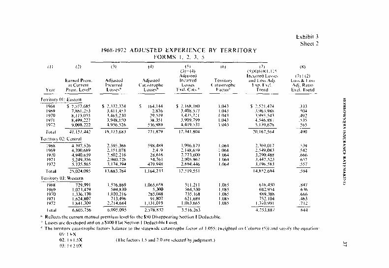
Exhibit 3 Sheet 2

1968-1972 ADJUSTED EXPERIENCE BY TERRITORY FORMS I, 2. 3. 5

0) (3) (3) (4) (5, (3)-(4)

AdJlWd Incurred LC%\CZ\

I-WI. Cill\.b

(71 (S)X(h)Xl.l IS Incurred Lo\w and I.<>\\ Ad).

Exp. trcl Trend

(X)

(7)1(2) LO\\ & Lo\\ Ad]. Ratw txcl. Trend

tarned Prem AdJu\wd .AdJu\trd al Current Incurred Catawophc

YGlr Prcm. Lcvcl’ Lo\\e\” LU\\C\b

Tcrritorv 01: Eatrrn -. 196X $ 7.517.685 I969 7.X61.253 I970 8. I I i.oss 1971 X.499.227 1972 9.09x.222

$ 7.332.374 3.41 I.453 3.465.230 3.94X. I so 4.956.52f1

s 164.144 2.X76

043 5 252 I.474 333 043 3.963.98X so4 043 3.Y95.543 4Y2 043 4.546,Xx I .s3s ,043 5.139.67X .Sh.i

.064 ,064 Oh4

s 2.lhX.IXO 3.40x.577 3.435.71 I 3.909.799 4.419.537

17.34 I .X04

I

7O.lh7.5hJ 490

I .996,X79 2.14X.659 2.773.600 2.YOZ.967 2.6Y4.446

12.519.551

,064 ,064

2.369.017 539 2.549.0x3 .542 3.290.48X ,666 3.447.523 .657 3.196.5X3 .557

14.X52.694 .594

51 I.21 I S64.530 735.168 62 I .6X9

I .0X3.665

I.085 I .0x5 I.085 I .oxs I.085

6 I X.450 6X2.954 889.388 752.104

1.310.991

3.5 16.263 4.253.8X7

29.5 I9 3X.351

536.989

771.X79 Toral 41.151.442 IX. 113.683

Terrnor) 02: Central

59X.489 2.419

2X.6 I6

196X 4.397.526 1969 4.700.689 I970 4.940.659

2.595.368 2.151.078 2.x02.2 I6 2.960.72X 3.174.394

13.683.784

1971 5:249.356 1972 5,735.X6.5

Total x.024.095

Terrnory 03: Wc\tern

196X 729.991 I969 I .073.479 1970 I .336. I70 lY7l 1972 1 h$g

A Total 6.605.756

54.76 I 479.9438

1.164.233

I .576.X69 x47 ,636 ,666 ,463

I .065.65X 5.300

2X5.048 9 I .X07

1.131.019

2.57X.X32

569.830 I .020.2 I6

7 I3.49h 2.2 14.684

6.095.095

.712

,644

’ Rrllwt~ the current manucll prcmlum Icvel ior the 650 Disappearing Section I Deductlblc. b Lo\>r\ are dcvcloped and on a SIOO Flat Scctwn I Dcductlhlc Level. c Thr trrrnory catastrophe factor\ balance to the \tatrwldc catastrophe ljctw or I.05 (uelghtrd on Column (5)) and saw)- the equation:

01: 1+x 02: I + I.SX (The l’actor\ I.5 and 2.0 are wlrcted h) judgment.) 03: I +2.0x


Exhibit 4

STATEWIDE DEVELOPMENT OF INDICATED RATE LEVEL CHANGE-TENANTS ~FORM 4

(1) (2) 0) (4) LOSSES INCL.

LOSSES LOSS ADJUSTED ADJUSTED TO ADJUSTMENT CURRENT

EARNED SIOO FLAT EXPENSE COST YEAR PREMIUMS DEDUCTIBLE” (2)Xl.I I5 FACTOR

1968 $ 588,318 $ 231,267 $ 257,863 I969 698,673 302, IO9 336,852 I970 837,047 395,424 440,898 1971 I .046,955 499,867 557,352 1972 1.184.752 529,937 590,880

(5) (6) LOSSES ON TRENDED

CURRENTCOST LEVEL INCURREDLOSSES YEAR (3)X(4) (5)X 1.062”

I968 $ 323,876 $ 343,956 I969 399,170 423,919 I970 491,160 521,612 1971 594,695 63 I.566 I972 609, I97 646,967

(WEIGHTED .lO, .15, .20, .25, .30)

I.256 I.185 I.1 I4 I .067 I .03 I

(7) ADJUSTED

10% RATIOS (6)/(l)

.585

.607

.623 ,603 ,546

,589

(8) Indicated Premium Level Adjustment for $100 Flat Section I Deductible from Present Deductible optionsc: .589 t .602 = .973 (= -2.2%).

(9)

Present Deductible

Options

Full Coverage $50 Dis. Ded.

(10)

Present Average Premium

Level

I .250 I .ooo

(II, (12) Indicated SlooFlat (11)+(10)-1 Section I AkW+?c Premium Premium

Level Change

I .063 - 15.0% I .063 + 6.3%

- 2.2%

(13) (14) Current

Premium Dktributlon

b Deductible

17.1% 40% 10.9% 60%

13.44’ 100%

(15) Indicated Rate Level Change = + I 2.9RJ 1.978 t ( I .OOO - ,134) = I.1291

n Average Loss Elinination Ratio (for 5 year period): I I2

b Factor to adjust lose3 on current cost level to 4/ I /75. c Balance Point Loss Ratlo: ,602.


Appendix A Sheet I

$100 FLAT DEDUCTIBLE LOSS ELIMINATION RATIO SUPPLEMENT

This memorandum explains the analysis and development of loss elimination ratios (LER’s) recognizing the effect of a $100 Flat Deductible. LER’s can be developed from a study of accident year loss data from a large sample of companies. The data consists of claims which are broken down by form, by deductible, by cause of loss and by size of loss. This is the basis for the computation of a $100 Flat Section I Deductible LER, i.e. the percentage of loss eliminated in converting full coverage losses to losses payable under a $100 Flat Section I deductible. The following example is a step by step development of a $100 Flat Section I Deductible LER for Form I Cause of Loss+ Fire.

PART I

The data shown on Sheet 2 is an extract of the data underlying the development of the aforementioned LER for Form I, Cause of Loss Fire. This extract represents Homeowners Policy Form I. Deductible Code 1 (Full Cover). Cause of Loss--Fire; and shows the number and amount of losses broken out by size intervals (as shown below).

Formula ldcntification

Size of Loss Intervals’

.oQ- I .77 I .78- 3.15 3.16s 5.61 5.62- 9.99

lO.OO- 17.77 17.7% 31.61 3 I .62- 56.22 56.23- 99.99

loO.OO- 177.82 177.X3- 316.22 3 I6.23- 562.33 562.34- 999.99

lOCO.OO- 1778.27 1778.2% 3 162.28 3 l62.29- 5623.37 5623.3% 9999.99

10000.00-17782.79 177X2.80-31622.84 31622.x5-56233.74 56233.75-99999.99

1OOOOO.00 and above

Sire of Loss

Code

:, 7 u 9

IO I I I2 I3 I4 I5 16 17 18 I9 20 21

Number of Lose\

:: E.i Ii:, 1,: N9 NIO NII NI2 Nl3 N14 Nl5 Nl6 N17 Nl8 N19 N20 N2I

Amount 01 Loses

LI L2 L3 L4 L5 L6 Ll LX L9 LIO LII LIZ Ll3 L14 Ll5 Llh L17 LIX L19 L20 L2I

n Interval\ selected from logarithmic scale (as sile of lo\\ distribution\ are often lop-normal)

40 HOMEOWNERS INSURANC’E RATbMALlNC.

Appendix A Sheet 2

LER SUPPLEMENT

HOMEOWNERS HO- 1

FUL.L COVER, CAUSE ok Loss FIRI:

SIZE OF LOSS INTERVAL CODE(X)

NUMBEROF LOSSES(N)

AMOUNT OF LOSSES(L)

I 2 3 4 5 6 7 8 9

IO II 12 I3 I4 I5 I6 I7 18 I9 20 21

I51 4.05 14 38.65 93 435.77

228 I 806.39 736 10033.3 I

I I59 28078.54 1225 5266 I .88 I I20 86978.56 821 110678.75 636 149308.8 I 396 167214.81 257 192336.19 I57 198823.3 I 96 224101.44 71 306616.31 75 574609.3 I

100 1280350.00 22 490346.25

1 42574.00 I 66000.00 0 0.0

Summary of above Data:

; Lx = Sum of the amount of losses under x= I $100.00 =

21

z Lx = Sum of the total amount of losses = x= I

21

z NX = Sum of the number of losses for loss

x=9 amounts greater than or equal to $100.00 =

$ 180,037

$3,982,996

2,633

HOMEOWNERS INSURANCE RATEMAKING

LER SUPPLEMENT

PART 2

41

Appendix A Sheet 3

The following sets forth the formula for development of the Loss Elimina- tion Ratio on a $100 flat basis and shows its application to the data summarized in Part I. The Loss Elimination Ratio developed is .083 for the peril of Fire under Form I. The same formula is used for other causes of loss under Forms I, 2, 3 and 5.

ii Lx +$ioo ; NX X=l x=9 = LER

21

x Lx X=l

The $100 Flat Deductible Loss Elimination Ratio formula described:

LER $100 flat deductible loss elimination ratio

= equals

; Lx (a) the elimination of all losses under $100.00

x= I

+ plus

$100 ii Nx (b) the elimination of $100 of every loss over $100.00 x=9

2 divided by

21

= Lx the total amount of losses. X=l

The application of the formula to the data summarized in Part I develops the LER for Form I, Cause of Loss Fire:

LER = $180,037 + [$I00 x 2,633] $443,337

$3.982.996 = $3,982,996 = “‘I

Tempered LER: .I11 x.75 = .083

The LER’s are tempered to recognize the prospective change in loss settle- ment patterns resulting from increasing the size of deductibles for insureds.

Accident

Year

LOSS DEVELOPMENT SUPPLEMENT

Factor

I51027 Months

Statewide

Countrywide

1968 1969 1970 1971

Weighted Average

1968 1969 1970 1971

Weighted Average

1.041595 I .032352 I .017355 I.01 1214

Factor 27 to 39

Weight Months - -

.07 I .007904

.27 I .006483

Factor 51 to63

Weight Months Weight - - -

.20 .996567 1.00

.80 .33 .33

.992399

Factor 39 to 5 I

Weight Months --

.10 I .002720

.40 I .005274

.50

I .02 1074

I .028596 I .025400 I .026445 I .02 1209

.07

.27

.33

.33

.999583 I .004763

.000352 .I0 .998903

.000585 .40 I .0005 I8

.003333 .50

$ g .996567

.? 2

.20 I .oooooo 1.00

.80 g

E r 3

I .024586 I .001936 1.000195 I .OOOOOO

Applicable to Accident Years

1968 (63 months to ultimate) 1969 (5 I months to ultimate) 1970 (39 months to ultimate) 1971 (27 months to ultimate) 1972 (I5 months to ultimate)

“State factor used for I.5 to 27 months and Count!

,000 .ooo: .ooo: .002: .023:

Selected Factors

Factors

Appendix B ft

I .OOOOOO = (5 I to 63 months) x (63 months to ultimate) I .000195 = (39 to 5 1 months) x (5 I months to ultimate) I.002 I3 I = (27 to 39 months) x (39 months to ultimate) I .023250 = (I 5 to 27 months) x (27 months to ultimate)

wide Factors for 27 to 63 months


Appendix C Sheet I

STATEWIDE

DERIVATION OF CATASTROPHE FACTOR BASED ON 1953-1972 EXPERIENCE

(1) (2) (3) Catastrophe Normal

Serial Numbered Homeowners Wind Losses

LOSSIZS Wind Lo\\rs m-(1)

1953-1967” Dwelling ECE Losses $ 2,544,426 $26.362.835 $23,818,409 1957-1972 Homeowners Losses I I, 126,556 26,982,744 15,856, I88

Total $13.670,982 $53,345,579 $39.674.597

(4) Loading for Catastrophe = Total ( I )/Total (3) = .345

(5) Provision for Cats. = (4) X Homeowners (3) = $15,856, I88 X ,345 = $5,470,385

(6) Total (All Causes) Homeowners Losses 1957-1972 = $I I 1,070,095

(7) Total (All Causes) Normal HO Losses 1957-1972 = (6) - Home- owners ( I ):

$I I 1,070.095 = (6) ll,l26,556 = Homeowners(l)

99,943,539 = Total Normal HO Losses 1957-1972

(8) Catastrophe Factor for Normal Homeowners Losses = I + ((5)/(7)):

, + $ 5,470,385 = 1.055 $99,943,539

e After 1967 Dwelling EKE is conrIdered 3 truly residual coverage.

44 HOMEOWNtRS INSL:HANC t RATbVAKlSC,

.\ppcndix C Sheet 7

Dl-IRIVATION OF STATEU’lDt’ C‘IVII. l>ISC)RDl:R l- s\CTOR

(1)

(2)

(3)

(4)

(5)

(6)

(7) (8)

BASED ON 1965-1977 kXPERII:NC‘b

Statewide Reported Loxscs (1965-1072) (Forms I, 2. 3.5) $ hY,Oh5,557

Statchide Rcportcd Catastrophe LUMCS. Including Riot and Civil Disorder Losses 7, I3Y.025

Statwide Normal Losses: (I) - (2) 0 I .Y26.532

Stutwidc Kcportcd Riot and C‘ivil Disorder Lossus Il.103

Statwide Civil Diwrdcr Potential: (4) t (3) .0002

Stateuide Civil Disorder Factor: (5) \ub.jcct IO m;tKi- mum and minimum” .OOO’

Statewide Catastrophe b’actor (l‘rom Sheet I ) I.055 Statcu idc Catastrophe Factor. Including Civil Dis- order Factor: (6) + (7) (Rounded to three decimal place) I.055

DEVELOPMENT OF CURRENT COST FACTORS (CSF) AND TREND FACTOR FOR FORMS 1,2,3,5

Appendix D Sheet I

QUARTER ENDING JUNE 30. 1973

PART A: ESTABLISHMENT OF MONTHLY COMPOSITE CURRENT COST INDEX (CCCI). WITH:

60% WEIGHT TO BOECKH RESIDENTIAL CONSTRUCTION COST INDEX 401 WEIGHT TO MODIFIED CONSUMER PRICE INDEX (MCPI)” (BOECKH BASE: l967= 100 MCPI BASE: 1967 = 100)

1970 1971 1972

3 MOS. 3 MOS. 3 MOS. MO. BOECKH MCPI ccc1 AVG. BOECKH MCPI cccl AVG. BOECKH MCPI ccc1 AVG. -P---------P-

7 123.6 118.1 121 4 135.6 123.5 130.8 146.7 127.5 139.0 8 123.9 11X.7 171.8 136.3 123.9 131.3 147.6 127.7 139.6

9 125.1 119.5 122.9 122.0 137.5 124.5 132.3 131.5 148.3 128.5 140.4 139.7

IO 125.3 120.2 123.3 137.5 124.9 132.5 148.8 128.9 140.8 II 126. I 120.9 124.0 137.5 125.3 132.6 149.3 129.3 141.3 I2 126.2 121.4 124.3 123.9 137.5 125.6 132.7 132.6 149.6 129.6 141.6 141.2

1971 1972 1973

3 MOS. 3 MOS. 3 MOS. MO. BOECKH MCPI ccc1 AVG. BOECKH MCPI ccc1 AVG. BOECKH MCPI cccl AVG. -- ~-- -- ~----

I 126.4 121.4 124.4 140.1 125.6 134.3 149.7 129.4 141.6 2 126.6 121.5 124.6 141.9 126.0 135.5 151.4 129.9 142.8 3 128.5 121.6 125.7 124.9 142.X 126.3 136.2 135.3 154.7 130.4 145.0 143.1

4 129.7 121.9 126.6 143.7 126.7 136.9 1.57.3 131.0 146.8 5 129.1 122.7 126.9 144.6 127.1 137.6 159.2 131.6 148.2

6 130.3 123.2 127.5 127.0 145.6 127.4 13X.3 137.6 160.3 132.0 149.0 148.0

6

DEVELOPMENT OF CURRENT COST FACTORS (CSF) AND TREND FACTOR FOR FORMS I, 2,3,5

Appendix D $ Sheet I

QUARTER ENDING JUNE 30, 1973

PART 8: USE OF AVERAGE ANNUAL CCC1 TO CALCULATE CURRENT COST FACTORS (CCF)

CALENDAR YEAR AVERAGE CCC1 CURRENT COST FACTORS BASED ON AVERAGE CCC1 VALUE FOR

YEAR BOECKH MCPI cccl QUARTER ENDING JUNE 30, 1973 = 148.0 - - - - m 1968 107.3 104.7 106.3 148.0/ 106.3 = I.392 I969 116.2 I I I.0 114.1 148.0/114.1 = 1.297

;

I970 122.4 11X.0 120.6 148.0/120.6 = I.227 ,” a 1971 132.X 123.3 129.0 148.0/129.0 = I.147 z I972 145.x 127.6 138.5 148.0/13&i = 1.069 F

P :

a Modified Consumer Price Index (MCPI) = comhinatwn oi following ~trms in Consumer Prw Index (with urlphth 60%. ?O%, 107 ; and 10%): housing. apparel. recreation and medlcal care. 5

; ; z c:

HOMEOWNERS ,NSURANCE RATEMAKING

PART C: COMPUTATION OF LOSS TREND FORMS 1, 2, 3. 5

AVERAGE CALENDAR QUARTER TIME cccl

YEAR ENDING (2X) (Y) --

I970 1970 1971 1971 1971 1971

1977 1972 1972 1972 1073 iY73

EQUATIONS:

SEP. 30 -II 122.0 DEC.31 -9 123.9

MAR. 31 -7 124.9 JUN. 30 -5 127.0 SEP. 30 -3 131.5 DFC.31 -I 132.6

MAR. 31 I 135.3 JUN. 30 3 137.6 SEP. 30 5 139.7 DEC. 31 7 141.2

MAR. 31 Y 143. I JUN. 30 I I 14X.0 --

0 1606.X Y=A+BX

SY = NA + BSX SXY = ASX + BSX’

47

Appendix D Sheet 2

FACTOR FOR

(ZXY) (4X?) - - - 1342.0 121 -1115.1 Xl

-874.3 49 -635.0 25 -394.5 9 - 132.6 I

135.3 I 412.X Y 698.5 25 98X.4 40

1287.9 XI 1628.0 121

657.4 572

WHERE A = MEAN OF FITTED LINE B = AVERAGE QUARTERLY

INCREMENT S = SUMMATION N = NUMBER OF OBSt~RVATIONS

2SXY = 657.4 OR SXY = 328.70

4SX’ = 572 OR SX’ = I43

A(MEAN OF FITTED LINE) = 1606.X/I’ = 133.90

B(AVG. QUARTERLY INCREMENT) = 32X.70/142 = 2.299

AVG. ANNUAL INCREMENT = 4 X 2.299 = 0.20

FITTED CCC1 TREND AT MIDPOINT OF QTR. ENDING JUNE 30, 1973 = 133.90 + (5.5 X 2.299) = 146.54

L:ZTFST ANNUAL RATE OF CHj\NGE = Y.20/146.54 = 6.3”(

48 HOMEOWNERS INSLIRAN( k RATEZlAKIN(i

[Ippcndix D Sheet 3

CALCULATION OF CURRENT C‘OST/AMOUNT f-‘A<‘TORS

(FORMS I. 2. 3, 5):

(1)

l’h4K

I71

ILI,K,\(;t, K t I \-Fll IT\‘”

1968 I Yh9 1970 I97 I 1972 5- 15-73

I.292 I .34x I.415 I .500 I.562 I .64Xb

0)

KI:I.-\~IlI’I 11 TO l..47kST

POINT (2) (1973)+(z)

(4) C’I~KKbhl

~41\10I~N 1 I ‘4C IOK (3).1 t hll’t Kt.1)

X5’ I I((?)kI)x.x5J+ I

I.276 I .735 I .223 I. I90 I.165 I I30 I.099 I .0X4 I.055 I.047 I ,000 I .ooo

(il

(‘I KK1.N I I (‘OST

I :\C’ I OK’

I .3Y2 I.297 I .‘27 1.147 I .OOY

C UKKt:NT : OSI/:\M~r

k .4C TOK (5) t (4)d

I.127 I .090 1.076 I .05x I .o:! I

CALCULATION OF TREND~D(‘OSTiAMOUN’1 FACTOR

(FORMS I, 2, 3, 5):

Latcxt Annual Rate of‘ Change of‘ Average Relativitics (I‘rom Column (2) above) = 4.4%

Tempered 75”( = 3.3’; = R

C = Latest Annual Rate 01‘ Change of’ 1.c~ Cost ( Icrom Sheet 2) = 6.3%’

I + <‘ = Latch1 Annual Rate of’ C‘hanyc In 1.0~s Ratios = 1.02Y (=Z.Y’&)

I+R

Modil‘ied Trend Factor to Adjust Loss Ratio to ;I -I/ I ,/75 Icvclr from 5/I i/73”:

I + (.029 x Ih.‘) + (.Oh3 x -+’ = I .07 I I~


Appendix D Sheet 4

DEVELOPMENT OF CURRENT COST FACTORS (CCF) AND TREND FACTOR FOR FORM 4

QUARTER ENDING JUNE 30, 1973

PART A: ESTABLISHMENT OF QUARTERLY AVERAGE OF

MODIFIED CONSUMER PRICE INDtX (MCPI)

(MCPI BASE: 19h7 = 100)

1970 1971 1972

3 MOS. 3 MOS. 3 MOS. MONTH MCPE AVG. MCPI AVG. MCPI AVG.

7 Il8.1 123.5 127.5 8 118.7 123.9 127.7 9 119.5 118.8 124.5 124.0 128.5 127.9

10 120.2 124.9 128.9 I I 120.9 125.3 129.3 I2 121.4 120.8 125.6 125.3 129.6 129.3

1971 1972 1973

3 MOS. 3 MOS. 3 MOS. MONTH MCPI AVG. MCPI AVG. MCPI AVG.

1 121.4 125.6 129.4 2 121.5 126.0 129.9 3 121.6 121.5 126.3 126.0 130.4 129.9

4 12 1.9 126.7 131.0 5 122.7 127. I 131.6 6 123.2 122.6 127.4 127.1 132.0 131.5

PART B: USE OF AVERAGE ANNUAL MCPI TO CALCULATE CURRENT

COST FACTORS (CCF)

CALENDAR YEAR AVERAGE MCPI CURRENT COST FACTORS BASED ON AVERAGE MCPI VALUE FOR

YEAR MCPI QUARTER ENDING JUNE30. 1973 = 131.5

1968 104.7 131.5/104.7 = 1.256 1969 111.0 131.5/l I I.0 = 1.185 1970 118.0 131.5/l 18.0 = I.114 1971 123.3 131.5/123.3 = 1.067 1972 127.6 131.5/127.6 = 1.031

50 HOMEOWNERS INSURANCE RATEMAKINC.

PART C: COMPUTATION OF TREND FACTOR FOR FORM 4

CALENDAR QUARTER YEAR ENDING

1970 SEP. 30 1970 DEC. 31 1971 MAR. 31 1971 JUN. 30 1971 SEP. 30 1971 DEC. 31

1972 MAR. 31 1972 JUN. 30 1972 SEP. 30 1972 DEC. 31 1973 MAR. 31 1973 JUN. 30

EQUATIONS: Y= SY =

SXY =

TIME

(2x1

-II -9 -7 -5 -3 -I

I 3 5 7 9

II

0

A + BX

AVERAGE MCPI

(Y)

118.8 I2O.X 121.5 122.6 124.0 125.3

126.0 127. I 127.9 129.3 129.9 131.5

1504.7

NA + BSX ASX + BSX?

Appendix D Sheet 5

(2XY) (4X?) - - - 1306.X 121 -1087.2 81

-850.5 49 -613.0 25 -372.0 9 - 125.3 I

126.0 I 381.3 9 639.5 25 905. I 49

1169.1 81 1446.5 121 -- - 312.7 572

WHERE A = MEAN OF FITTED LINE B = AVERAGE QUARTERLY

INCREMENT S = SUMMATION N = NUMBER OF OBSERVATIONS

2SXY = 312.7 OR SXY = 156.35

4SX? = 572 OR SX? = 143

A(MEAN OF FITTED LINE) = 1504.7/12 = 125.39

B(AVG. QUARTERLY INCRbMENT) = 156.35/143 = 1.093


Appendix D Sheet 5

PART C: COMPUTATION OF TREND FACTOR FOR FORM 4

AVG. ANNUAL INCREMENT = 4 X 1.093 = 4.37

FITTED MCPI TREND AT MIDPOINT OF QTR. ENDING JUNE 30, 1973 = 125.39 + (5.5 x 1.093) = 131.40

LATEST ANNUAL RATE OF CHANGE = 4.37/131.40 = 3.3%

TREND FACTOR TO ADJUST LOSSES” TO A 4/I /75 LEVEL FROM 5/15/73:

22.5 I + (.033 x12 ) = 1.062

BLosses only we projected because Form 4 is an Actual Cash Value coverage on depreciating contents values, not wbject to the same inflationary pressure 3s that on replacement cost for building values.

52 HOMEOWNERS INSURANC’F RATEMAKINC)

Appendix E

REVISION OF HOMEOWNERS INSIJKANCE Rt!LATIVITY CURVE

CALCULATION OF PREMIUM OFF-BAI.AN(.F R~\L,I TIN{; FROW

INTRODUCTION OF NEW RELATIVITY Cc KVI. HI ,AMOI. NT 91 ISSL’RANCI.

ILLUSTRATION: FORM HO-2 SnT1~wll)f~ OI,I,-BAI ANCI,

,Amount 01 Inwrtincr

(In $1.000’~)

08-I’

13-17 18-22 23-27 28-32 33-37 38-42 43-47 48-52 53-57 58-62 63-67 68-72 73-77 78-99

TOTAL

7.2%’ .X6 .X6 l6,9?k I .oo I .oo 29.54’ 1.24 I .24 16.0%~ I.55 I .57 12.3% I .90 2.01 8.0% 2.30 7.44 4.77 2.70 2.X0 1.6%’ 3.10 3.x I .2’S’ 3.50 3.70 I .O%’ 3.90 4.17 .4%’ 4.30 4.54 .3%’ 4.70 4.96 .30/(’ 5.10 5.3x

I%’ 5.50 5.x0 .40/c’ 7.41 7.82

100.077 I.607 I.656

OFF-BALANCE = 1.656/1.607 = 1.030. THE OFF-BAI.ANCE IS THE PREMIUM LEVEL CHANGE RESULTING FROM APPLICATION OFTHE NEW RELATIVITY CURVE WITH NO CHANGE IN UNITY (Sl5,OOO AMOUNT OF INSURANCE) PREMIUMS. TO PRODUCE NO PREMIUM LEVEL CHANGE, THE FORMER UNITY PRE- MIUMS MUST BE DIVIDED BY THE OFF-BAl./\NCE.

“(5) = 1((4) + (3)) + OFF-BALANCE] - I .O


Appendix F Sheet I

REVISION OF HOMEOWNERS INSURANCE FORM RELATIVITIES

This deals with the introduction of premium rclativities by Form. In addition to simplifying future experience reviews, the establishment of uniform relationships between forms should facilitate machine rating of Homo- owners policies. Sheets 2 and 3 show the development of the new relativitics.

Column I of Sheet 2 is the current average relativity of Forms I, 2, and 5 to Form 3 at the unity premium as shown on Sheet 3 (assuming all Forms are on the same policy size relativity curve).

Column 2 is the rate level increase which would result from the intro- -- duction of the new policy size relativity curve with no change in unity premiums. (See Appendix E.)

Column 3 Statewside loss ratios by Form balance to the combined adjusted loss ratio, as dcvclopcd on Exhibit I.

Column 4 shows the arithmetic “indicated” loss ratios by Form at Form -- 3 rates. excluding credibility considerations.

Column 5 makes Form 3 the base Form. and contains “indicated” Form relativities.

Column 6 shows the new Form relativitics, selected by judgment in comparing Columns (I) and (5). bearing in mind the volume of data implied by Column (7).

Column 7 ix the current distribution of premiums by Form.

Sheet 3 shows the current average form relativitics by territory and statewide.

The new Form rclativitics for this state arc:

Form I: I .70

Form 2: .85

Form 3: I .oo

Form 5: I .40

Appendix F Sheet 2

POLICY FORM RELATIVITIES

(II (2) (3) (4) (5)

Form

I

2

3

5

Current Off-Balance

Avrrallr of Rwkd

Form R&itlVll~

Reiatw~ty~ Cur&

,652 I.014

,871 I.030

I.000 I.047

I .630 I .055

5 Year .Adjustrd

Loa\ Ratio

.8l I

.65 I

.7lO

.606

Induted LCM R&b at Form 3 Rata (31X(l)+-(l)

,521

35 I

,678

,936

Rrlatwn!, ol Lo\\ Ratio\ to Form 3

.76X

.813

I.000

I .38 I

z (6) (7) g

1977 Form s Distrlhutmn 01 5

Selected Adjusted z Form Earned 2

2 Relatw> Prcmlum a

% .70 ,309 $

r .85 ,468 ;:

z I .oO ,201 ; I .40 .027 ;


Appendix F Sheet 3

CURRENT AVERAGE FORM RELATIVITIES BY TERRITORY

Territory

01

02

03

STATEWIDE

Form

I 2 5

I 2 5

I 2 5

I 2 5

Current Average Relativity

(to Form 3)

,648 ,866

I.582

.657 ,882

I .663

,650 ,867

I.624

.652

.87l 1.630

New Form

Relativities

.70 ,115

I .40

.70

.85 I .40

.70

.85 I .40

.70

.85 I .40

56 HOMEUWStRS INSURANC t RATt>lAKIN(i

Appendix F Sheet 4

CALCULATION OF REVISED MANUAL PREMIUMS AT $15,000 (UNITY)

The revised manual premiums are developed using the formula shown below:

PREL. ~AEPiXOB,X~X(I+R)=I+X

I

Wherei= l,2,3,and5

AEPi = 1972 Adjusted Earned Premium for Form i as a percentage to total for Form\ I, 2. 3, and 5.

OBi = Off-Balance of Form i which is the result of introducing a new relativity curve. (Set Appendix E)

PR EL i = New relativity of Form i to Form 3 a! $15,000 (See Page F-3.)

CREL; = Current average relativity of Form i to Form 3 at $15,000. (See Page F-3.)

R = Change to Form 3 Broadest Deductible unity premiums to go to $100 Flat Option.

X = Overall change to Forms I , 2, 3, and 5 Broadest Deductible unity premiums to go to $100 Flat Option.

As an example, the development of the revised unity premiums for a $100 Flat Section I Deductible for Premium Group I follows: (Pre- mium Group I = Territory 01. Brick. Protection Class 2)

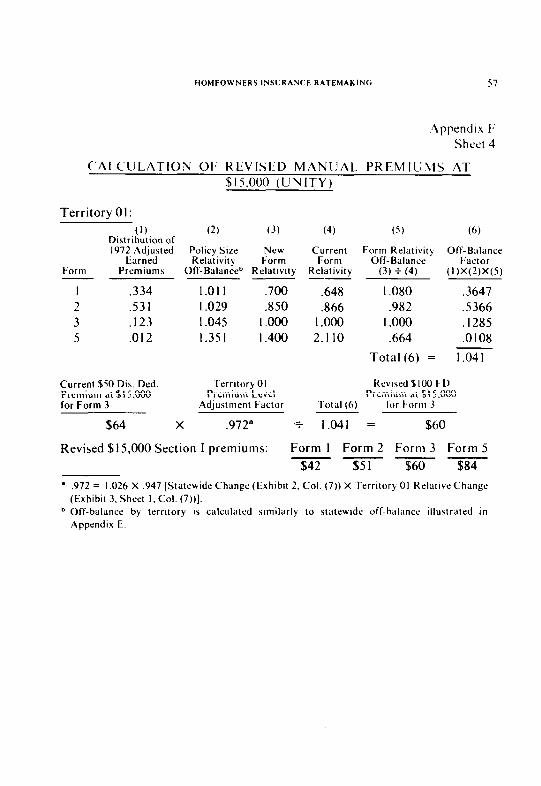
HOMEOWNERS INSL’RANCE RATEMAKINC 57

,Appendix F Sheet 4

CALCULATION OF REVISED MANUAL PREMIUMS AT $15.000 (UNITY)

Territory 01:

(1) Distribution of 1972 Adjusted

Earned Form Premiums

I .334 2 .53 I 3 ,123 5 .OI2

(2)

Policy Sire Relativity

Off-Balance”

I.01 I I .029 I .045 I .35 I

(3) (4) (5) (6)

NW Current Form Relativity Form Form Off-Balance

Relativity Relativity (3) + (4) - --

,700 .648 I .080 ,850 .866 .982

I.000 I .ooo I .ooo I.400 2. I IO .664

Total (6) =

Off-Balance Factor

(1 )X(2)X(5)

.3647

.5366

.I285

.OlO8

I.041

Current $50 Dis. Ded. Territory 01 Revised $ IO0 FD Premium at $15.000 Premium Level Premium iit $15.000 for Form 3 Adjustment Factor Total (6) for Form 3

$64 X ,972” -+ I.041 = $60

Revised $15,000 Section I premiums: Form I Form 2 Form 3 Form 5 - - - - $42 $51 $60 $84

’ ,972 = 1.026 X ,947 (Statcwide Change (Exhibit 2. Cal. (7)) X Territory 01 RelativeChange (Exhibit 3. Sheet I. Col. (7))].

b Off-balance by territory is calculated similarly to statewide off-halancc illustrated in Appendix E.

homeowners insurance ratemaking

Documents