home health care routing and scheduling with consistencyatoriello3/hhcrs.pdf · health care routing...
TRANSCRIPT

Home Health Care Routing and Scheduling withConsistency
Seyma Guven-KocakH. Milton Stewart School of Industrial and Systems Engineering, Georgia Institute of Technology, Atlanta, GA, USA,
Aliza HechingCompassionate Care Hospice, Inc., Burlington, NJ, USA, [email protected]
Pınar Keskinocak, Alejandro TorielloH. Milton Stewart School of Industrial and Systems Engineering, Georgia Institute of Technology, Atlanta, GA, USA,
[email protected], [email protected]
This work addresses a real-world home health care routing and scheduling problem (HHCRSP) faced by a
home care agency in the United States. In home health care scheduling, there is a desire to retain consistency
with respect to the home health aide servicing each patient; this consistency is referred to as continuity of
care. To address this preference for continuity of care, we propose a rolling horizon approach to the routing
and scheduling problem and introduce the consistent home health care routing and scheduling problem
(Con-HHCRSP). We present two different constructive methods to solve HHCRSP on a daily basis: an
integer programming-based method with approximations and a variant of a petal heuristic. We present
adjustments on these methods to address Con-HHCRSP, where the goal is to be able to quantify and control
the deviation of the new schedule suggested each day from the existing schedule in place, so that some of
the existing assignments may be retained in the new schedule that is produced. We discuss the performance
and computational efficiency of these methods.
Key words : Home health care services, assignment, routing, scheduling, consistency
1. Introduction.
Due to the increasing average age of the population, especially in developed countries, there is
a growing need for long-term medical care and assistance for elderly people. It is advantageous -
both to providers and to patients - to provide this care in the patient’s home as long as possible.
For providers, a long-term stay in hospitals or nursing homes is more costly than providing care
and assistance to patients in their homes. Meanwhile, patients feel more comfortable in their own
homes, resulting in improved quality of life. Therefore, programs for aging in place, which include
an individual’s freedom to choose the place where he lives regardless of his age or level of ability,
are widely endorsed by social and health services providers. The corresponding growth in home
1
Guven-Kocak et al.: Consistent Home Care Scheduling2
care services, i.e., services delivered outside of a structured setting, motivates the study of the
scheduling and routing of aides who visit patient homes.
Home care services vary with respect to the scope and structure of the care they provide. In
this work, we consider hospice care, which is aimed at relieving terminally ill patients from pain,
stress, and suffering. In the United States, in order for a patient to be hospice-eligible his physician
must certify that his expected remaining lifetime is less than six months if his condition were to
run its normal course. Hospice care focuses on pain management and improved patient quality of
life during this time period rather than focusing on curative care. We address a real-world home
health care routing and scheduling problem (HHCRSP) faced by a home care agency in the United
States. The agency has operated for more than two decades and has branches in over twenty states.
To lay out the details of the problem and provide effective solutions using real-world data, we
collaborated with one of the agency’s branches. The branch provides a number of different services
in accordance with the patient’s needs and plan of care including social work, nursing, and chaplain
visits. Patients are located in settings including their home, skilled nursing facilities, and assisted
living facilities, amongst others. The service most commonly provided is patient personal care;
this service is performed by home health aides (HHAs) who are trained and certified health care
workers.
Any proposed solution method to the routing and scheduling problem must consider the unique
characteristics of home care service. One of the most critical characteristics is that over time
each HHA develops a personal relationship with the patients and families he is servicing. As
such, there is a desire to retain consistency with respect to the HHA servicing each patient. This
consistency in care, referred to as continuity of care, serves to increase the overall patient quality
of care and patient and family satisfaction. Continuity of care allows a HHA to better monitor
patient status without loss of information. Further, patients perceive a better quality of service with
greater predictability and coherence (Haggerty et al. 2003). It is therefore desirable to maintain
consistency in the patient-aide assignments. This policy has usually been addressed in the literature
by developing models for a long planning period and keeping the aide-patient assignments consistent
over time. However, long-term planning increases computational complexity. Moreover, a long-term
scheduling approach is not appropriate in the hospice care setting, since there is a frequent need to
change the schedules. This is due to the nature of the hospice care environment, where a patient’s
expected remaining lifetime is less than six months. In fact, according to 2014 data, average patient
length of stay in hospice is approximately 70 days with a median of around 23 days and often is
as short as less than seven days (NHPCO 2016). Moreover, 28.2% of the patients leave the service
within 7 days, 26.5% of them leave within 30 days, and only 13.1% of them stays longer than 180
days (?). This fact reveals the need for adopting a rolling horizon approach in the solution method.

Guven-Kocak et al.: Consistent Home Care Scheduling3
The need for frequent schedule changes coupled with the desire to maintain continuity of care
motivates us to develop a solution method that updates an existing schedule rather than creat-
ing a new schedule from scratch. In this work, we present two different constructive methods to
solve HHCRSP on a daily basis: an integer programming-based method with approximations and
a variant of a petal heuristic. solutions. We also implement various improvement heuristics, such
as single swap, double swap, and combined single and double swap. Using our heuristic methods
for HHCRSP, we observed that the daily cost of operations is decreased by $3,250, which consti-
tutes around 42% improvement over the current schedule in operation. We present adjustments on
these methods to address the schedule updating problem, where the goal is to be able to quantify
and control the deviation from the existing schedule in place, so that some of the existing assign-
ments may be retained in the new schedule that is produced. We discuss the performance and
computational efficiencies of these methods.
The contributions of this paper are threefold. First, we introduce the consistent home health care
routing and scheduling problem (Con-HHCRSP). Second, to the best of our knowledge, this work
is the first to present solution methods and analysis for Con-HHCRSP for a multi-nurse problem.
Although continuity of care has been taken into consideration in the literature, the vast majority
of the proposed methods aim to create a long-term schedule with a consistency in the aide-patient
assignments without considering a dynamic approach. Finally, quantifying the deviation from the
prior period schedule will provide business decision-makers with a quantifiable measure of the
actual cost of the continuity of care policy and allow for relaxations or limitations in the policy
based on this cost analysis.
2. Literature Review.2.1. Home Health Care Problems
The Home Health Care Routing and Scheduling Problem (HHCRSP) can be seen as a variant of
a multi-depot, multi-vehicle routing problem (VRP) with various labor-related and time-related
constraints. However, HHCRSP has some aspects that are unique to scheduling and routing such
as a desire to retain consistency in the HHA-patient assignments, a need to assign HHAs with
preferred skills, and a need to consider specific labor-related constraints.
The uniqueness of the HHCRSP problem, coupled with the growth in home health services,
has resulted in a growing body of HHCRSP literature. Comprehensive literature reviews of home-
health care logistics problems and workforce scheduling problems can be found in (Gutierrez and
Vidal 2013, Castillo-Salazar, Landa-Silva, and Qu 2014, Fikar and Hirsch 2017). Many variants of
HHCRSP have also been studied. Some of the key differences between the problems are whether
HHAs are heterogeneous or homogeneous (e.g., with respect to skills, availability), length of the

Guven-Kocak et al.: Consistent Home Care Scheduling4
planning horizon (e.g., daily or weekly planning horizon), whether or not to consider time windows,
and the need to model simultaneous / interdependent visits. Moreover, the objective functions may
differ among the problems. Although most studies consider minimizing travel cost as a part of the
objective, some studies also consider maximizing HHA utilization, maximizing patient satisfaction,
or simultaneously optimizing multiple objectives.
In the home health care literature, we identified two papers that are most relevant to our work:
Bennett and Erera’s (2011) work on dynamic periodic fixed appointment scheduling, and Cap-
panera and Scutella’s (2014) work on joint assignment, scheduling and routing models with a
pattern-based approach. To the best of our knowledge, Bennett and Erera’s (2011) paper is the
first to consider a rolling horizon myopic planning approach to handle continuity of care in a home
health care context. However, our work differs from theirs in important aspects. First, they consider
a single-nurse case of the problem, while we propose solution methods for a multiple-nurse case
as the service areas of the nurses overlap in our problem setting. Second, they consider a weekly
schedule with a very strict requirement of consistency in the visit times by forcing the visit times
occurring on the same weekdays to be at the same time from week to week. On the other hand, we
focus on the consistency in nurse assignments, since, based on the information we obtained from
the home health care agency, we concluded that consistency in nurse assignments is critical in the
hospice care context. Third, they propose various heuristic methods to handle the problem, while
we propose both a MIP model and related heuristics, which means we can benchmark the perfor-
mance of one with the other. Lastly, we were able to use a real data set and had an opportunity to
see the performance and cost effectiveness of our methods in a real-world situation. Although their
randomly generated test instances mimic actual demand patterns observed at a sample real data
set, they do not test their methods on the real full data set to provide insights on the performance
of the methods in a real-world situation.
Cappanera and Scutella (2014) have made an important contribution to the home health care
literature by creating a joint model to handle assignment, scheduling, and the routing aspects
of the home health care problem. Although both our mathematical model for HHCRSP and the
model they propose consist of similar components, there are several aspects that differentiate our
work from theirs. First, they do not consider the consistency requirement in their work whereas we
place significant emphasis on this requirement in the current work. Although they aim to create a
weekly schedule where the continuity of care is ensured by keeping the nurse assignments the same
throughout the week, they do not consider preserving the consistency in the next period when
they need to re-optimize the schedule. We provide MIP models and heuristics both for HHCRSP
and Con-HHCRSP. Moreover, their MIP-based model is not able to solve some of the instances,
or may take a significant amount of time to solve some instances due to the complex nature of
Guven-Kocak et al.: Consistent Home Care Scheduling5
the problem. We propose both MIP-based model and heuristics to enable fast and high quality
solutions for a variety of instances. Therefore, our work has unique contributions in the context of
home health care problems as well as in a wider context of VRP where consistency may present as
an important component of the problem.
2.2. Consistent VRP
Consistency in the decisions made has been emphasized in many different contexts, with moti-
vations of customer satisfaction, improved operational planning, or convenience. Consistency
appeared in the VRP literature, after a shift in practice from cost-oriented operations to customer-
oriented operations (Groer, Golden, and Wasil 2009). Many companies prefer drivers to visit the
same customers at roughly the same time each time the customers require service, since this helps
drivers develop relationships with customers and leads to improved customer service (Wong 2008).
Groer, Golden, and Wasil (2009) first defined this problem as consistent VRP (ConVRP), where
the consistency constraints are combined with the traditional VRP constraints.
Kovacs et al. (2014) extended the consistent VRP by introducing the generalized ConVRP (Gen-
ConVRP), where they relaxed some of the strict consistency constraints. For example, they allowed
each customer be served by a limited number of drivers rather than a single driver and penalized
time inconsistency in the objective function instead of enforcing it by constraints. Similarly, in their
work on the multi-vehicle inventory-routing problem, Coelho, Cordeau, and Laporte (2012) con-
sidered various consistency features such as driver consistency, schedule consistency, and quantity
consistency, with a main motivation of increasing the quality of customer service. Moreover, Mac-
donald, Dorner, and Gandibleux (2009) defined a consistent nurse routing and scheduling problem
that considers care continuity over a given planning horizon.
In all of these studies, consistency is considered over a given planning period. In other words,
the period over which the consistency is required is determined and then the problem is modeled
and solved over this period. This idea is similar to the “continuity of care” concept that we have
introduced. However, this approach (defining the period over which consistency is required and
then solving the problem over this period) has some drawbacks. First, planning for a longer horizon
increases the computational burden. Second, implementing this approach may not be possible in
some practices where future data is unknown or uncertain (e.g., emergency cases introduce changes
to future data). In our context, the set of patients changes frequently due to both frequent patient
admissions and patient discharges (due to death). Further, there are many cases where a patient
is temporarily discharged from the system and no longer requires care (e.g., temporary transfer to
the hospital or a different care facility). Thus, a solution method that handles consistency for a
given planning period is not appropriate for these situations. Instead, we consider a rolling horizon
approach to address consistency preferences.

Guven-Kocak et al.: Consistent Home Care Scheduling6
To the best of our knowledge, only a few studies have used a similar rolling horizon approach.
Bennett and Erera (2011) considered a rolling horizon approach to handle continuity of care in a
home health care scheduling problem – but only for a single nurse. In our work, we propose solution
methods for multiple HHAs. In their work on dynamically scheduling aircraft landings, Beasley
et al. (2004) defined the ”displacement problem”, where the decision being made has a link back
to the previous decision, and ”displacement” refers to inconsistency in our context. Their main
motivation is the dynamic structure of airline planning and a need to change schedules each time
there is an information update. Although their ”displacement” concept is similar to our concept of
continuity of care, the two problems are very different in nature. One key difference is that their
aircraft scheduling problem does not include a routing component.
3. Problem Description and Model.3.1. Home Health Care Routing and Scheduling Problem (HHCRSP).
HHCRSP is a variant of a multi-depot, multi-vehicle routing problem with labor-related and time-
related constraints. We begin by describing the problem. Each day, each HHA is assigned a set
of patients that he must visit at scheduled times. The HHA travels from his home to deliver
care to his assigned patients in accordance with the assigned schedule. The HHA travels from
patient to patient; following completion of his daily assignments, the HHA returns home. We
consider deterministic travel times and distances between patient locations; these distances may
be calculated using a geographic information system tool. Service times are also considered to be
deterministic, having a value roughly estimated based on prior experience. In our problem setting,
we assume common service times across all patients.
Time-related constraints enforce regular working hours, i.e., these constraints enforce that all
visits begin no earlier than a specified start time and end no later than a specified end time. Labor-
related constraints are specific to the employee type: the workforce is comprised of part-time (PT)
and full-time (FT) HHAs and each is bound by different rules. FT HHAs are scheduled to work
a fixed number of hours per week; a FT HHA who works more than his regular scheduled hours
is paid for his excess hours at an hourly overtime rate. However, the sum of regular hours and
overtime hours may not exceed a maximum allowable number of working hours. PT HHAs are paid
at an hourly rate and may work up to a specified weekly regular number of hours with this hourly
rate. If a PT HHA works beyond the maximum number of permissible hours per week, then the
PT HHA must receive additional benefits such as insurance; the cost of these benefits is covered
by the employer. Our labor-related constraints are different from similar home health care routing
and scheduling problems discussed in the literature. Although most studies consider heterogeneous
aides (e.g., skilled nurses), this heterogeneity mostly affects the assignment decisions. In our case,

Guven-Kocak et al.: Consistent Home Care Scheduling7
the heterogeneity in cost calculations and time restrictions introduces additional complexity to the
problem.
In addition to the labor-related constraints, we consider patient preferences when assigning
patients to the PT and FT HHAs. Namely, patients may specify one or more HHAs that they
prefer and/or characteristics of HHAs that they prefer (e.g., gender, languages spoken). These
preferences are treated as soft constraints where a penalty is introduced to the objective function
for each preference violation.
Similar to the labor-related constraints, having soft constraints for the assignment decisions is
not common in the literature. In most cases, staff assignments are restricted due to hard constraints
such as skills requirements. Modeling preferences as a soft constraint and introducing a penalty
for preference violation introduces the challenge of appropriately selecting a penalty. Based on
discussions with the company, we note that patient preferences are seriously considered (as these
may directly impact customer satisfaction) but are balanced against costs incurred in meeting these
preferences. We therefore introduced these preferences as a soft constraint and impose a violation
penalty equal to an average cost of visiting a patient.
We now describe the mathematical model of HHCSRP using the notations presented in Table
1. The key model assumptions are (i) patients do not have time-windows, (ii) patients require
only one HHA to be present in a service visit, (iii) all visits to the same patient have the same
average duration, (iv) an HHA’s day begins when he arrives at his first patient and ends when he
leaves his last patient, and (v) part-time HHAs and full-time HHAs have different associated time
(availability) restrictions and labor costs.
min∑
g∈G,(a,b)∈Loc
cTygabDab +∑f∈F
cFγf +∑p∈P
cPwp +∑f∈F
cOFOf +∑p∈P
cOP θp +∑j∈J
λPPj
s.t.∑g∈G
xgj =∑g∈Gj
xgj +Pj = 1 ∀j ∈ J (1a)
∑j∈J
xgj ≤M ∀g ∈G (1b)
0≤ tgj ≤ (αH − sj)xgj ∀g ∈G, ∀j ∈ J (1c)
wg =∑i,j∈J
(Tij + sj)ygij +∑j∈J
sjyggj ∀g ∈G (1d)
γf ≥H −wf ∀f ∈ F (1e)
γf ≥ 0 ∀f ∈ F (1f)
Of ≥wf −H ∀f ∈ F (1g)
Of ≥ 0 ∀f ∈ F (1h)
Guven-Kocak et al.: Consistent Home Care Scheduling8
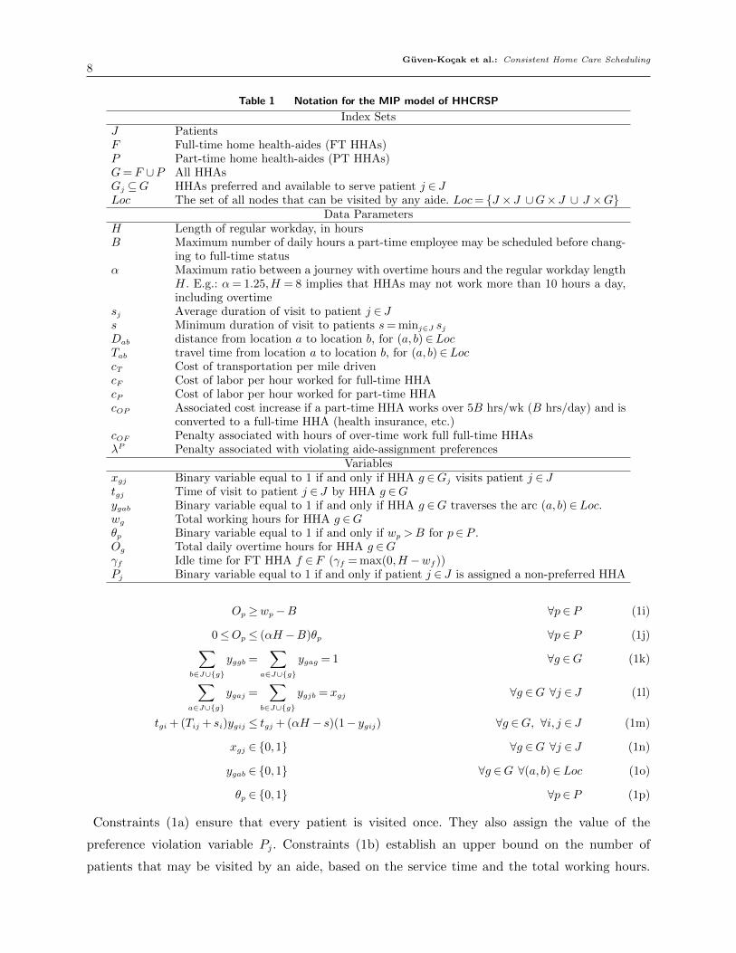
Table 1 Notation for the MIP model of HHCRSP
Index SetsJ PatientsF Full-time home health-aides (FT HHAs)P Part-time home health-aides (PT HHAs)G= F ∪P All HHAsGj ⊆G HHAs preferred and available to serve patient j ∈ JLoc The set of all nodes that can be visited by any aide. Loc= {J × J ∪G× J ∪ J ×G}
Data ParametersH Length of regular workday, in hoursB Maximum number of daily hours a part-time employee may be scheduled before chang-
ing to full-time statusα Maximum ratio between a journey with overtime hours and the regular workday length
H. E.g.: α= 1.25,H = 8 implies that HHAs may not work more than 10 hours a day,including overtime
sj Average duration of visit to patient j ∈ Js Minimum duration of visit to patients s= minj∈J sjDab distance from location a to location b, for (a, b)∈LocTab travel time from location a to location b, for (a, b)∈LoccT Cost of transportation per mile drivencF Cost of labor per hour worked for full-time HHAcP Cost of labor per hour worked for part-time HHAcOP Associated cost increase if a part-time HHA works over 5B hrs/wk (B hrs/day) and is
converted to a full-time HHA (health insurance, etc.)cOF Penalty associated with hours of over-time work full full-time HHAsλP Penalty associated with violating aide-assignment preferences
Variablesxgj Binary variable equal to 1 if and only if HHA g ∈Gj visits patient j ∈ Jtgj Time of visit to patient j ∈ J by HHA g ∈Gygab Binary variable equal to 1 if and only if HHA g ∈G traverses the arc (a, b)∈Loc.wg Total working hours for HHA g ∈Gθp Binary variable equal to 1 if and only if wp >B for p∈ P .Og Total daily overtime hours for HHA g ∈Gγf Idle time for FT HHA f ∈ F (γf = max(0,H −wf ))Pj Binary variable equal to 1 if and only if patient j ∈ J is assigned a non-preferred HHA
Op ≥wp−B ∀p∈ P (1i)
0≤Op ≤ (αH −B)θp ∀p∈ P (1j)∑b∈J∪{g}
yggb =∑
a∈J∪{g}
ygag = 1 ∀g ∈G (1k)∑a∈J∪{g}
ygaj =∑
b∈J∪{g}
ygjb = xgj ∀g ∈G ∀j ∈ J (1l)
tgi + (Tij + si)ygij ≤ tgj + (αH − s)(1− ygij) ∀g ∈G, ∀i, j ∈ J (1m)
xgj ∈ {0,1} ∀g ∈G ∀j ∈ J (1n)
ygab ∈ {0,1} ∀g ∈G ∀(a, b)∈Loc (1o)
θp ∈ {0,1} ∀p∈ P (1p)
Constraints (1a) ensure that every patient is visited once. They also assign the value of the
preference violation variable Pj. Constraints (1b) establish an upper bound on the number of
patients that may be visited by an aide, based on the service time and the total working hours.
Guven-Kocak et al.: Consistent Home Care Scheduling9
Constraints (1c) ensure that the visit times to the patient are zero if the patient is not visited and
non-zero if the patient is visited. Constraints (1d) calculate the actual working time in a day, which
is equal to the sum of travel times between patients plus visit durations. Constraints (1e) and (1f)
define idle time for full-time aides and restrict the idle time to be non-negative. Constraints (1g)
and (1h) define extra working hours for full time HHAs as total hours worked by the HHA minus
the number of hours FT HHAs are scheduled to work and restricts this value to be non-negative.
Constraints (1i) and (1j) sets the overuse indicator equal to one if working hours of a PT HHA
exceeds the maximum permissible number of hours per week. Constraints (1k) and (1l) are the
routing constraints for travel between patients. Each HHA will begin from home and return to
home as the start point and end point of his daily work “route”. Routing flows will be balanced.
Constraints (1m) enforce the start time of each visit to a patient to be later than the finish time
of the visit to the previous patient plus travel time and service time (when applicable). These
constraints also help eliminate subtours.
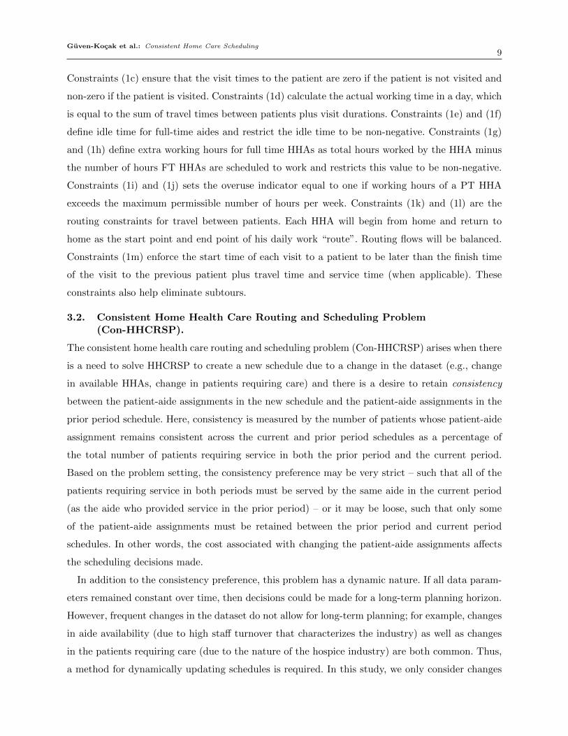
3.2. Consistent Home Health Care Routing and Scheduling Problem(Con-HHCRSP).
The consistent home health care routing and scheduling problem (Con-HHCRSP) arises when there
is a need to solve HHCRSP to create a new schedule due to a change in the dataset (e.g., change
in available HHAs, change in patients requiring care) and there is a desire to retain consistency
between the patient-aide assignments in the new schedule and the patient-aide assignments in the
prior period schedule. Here, consistency is measured by the number of patients whose patient-aide
assignment remains consistent across the current and prior period schedules as a percentage of
the total number of patients requiring service in both the prior period and the current period.
Based on the problem setting, the consistency preference may be very strict – such that all of the
patients requiring service in both periods must be served by the same aide in the current period
(as the aide who provided service in the prior period) – or it may be loose, such that only some
of the patient-aide assignments must be retained between the prior period and current period
schedules. In other words, the cost associated with changing the patient-aide assignments affects
the scheduling decisions made.
In addition to the consistency preference, this problem has a dynamic nature. If all data param-
eters remained constant over time, then decisions could be made for a long-term planning horizon.
However, frequent changes in the dataset do not allow for long-term planning; for example, changes
in aide availability (due to high staff turnover that characterizes the industry) as well as changes
in the patients requiring care (due to the nature of the hospice industry) are both common. Thus,
a method for dynamically updating schedules is required. In this study, we only consider changes
Guven-Kocak et al.: Consistent Home Care Scheduling10
in the set of patients requiring care and assume that the set of aides and other data parameters
remain constant.
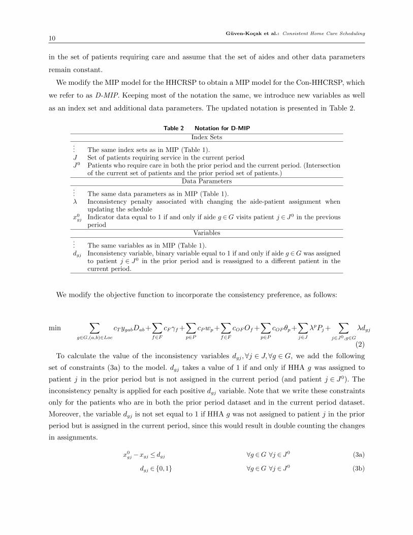
We modify the MIP model for the HHCRSP to obtain a MIP model for the Con-HHCRSP, which
we refer to as D-MIP. Keeping most of the notation the same, we introduce new variables as well
as an index set and additional data parameters. The updated notation is presented in Table 2.
Table 2 Notation for D-MIP
Index Sets... The same index sets as in MIP (Table 1).J Set of patients requiring service in the current periodJ0 Patients who require care in both the prior period and the current period. (Intersection
of the current set of patients and the prior period set of patients.)Data Parameters
... The same data parameters as in MIP (Table 1).λ Inconsistency penalty associated with changing the aide-patient assignment when
updating the schedulex0gj Indicator data equal to 1 if and only if aide g ∈G visits patient j ∈ J0 in the previous
periodVariables
... The same variables as in MIP (Table 1).dgj Inconsistency variable, binary variable equal to 1 if and only if aide g ∈G was assigned
to patient j ∈ J0 in the prior period and is reassigned to a different patient in thecurrent period.
We modify the objective function to incorporate the consistency preference, as follows:
min∑
g∈G,(a,b)∈Loc
cTygabDab+∑f∈F
cFγf +∑p∈P
cPwp+∑f∈F
cOFOf +∑p∈P
cOP θp+∑j∈J
λpPj+∑
j∈J0,g∈G
λdgj
(2)
To calculate the value of the inconsistency variables dgj,∀j ∈ J,∀g ∈ G, we add the following
set of constraints (3a) to the model. dgj takes a value of 1 if and only if HHA g was assigned to
patient j in the prior period but is not assigned in the current period (and patient j ∈ J0). The
inconsistency penalty is applied for each positive dgj variable. Note that we write these constraints
only for the patients who are in both the prior period dataset and in the current period dataset.
Moreover, the variable dgj is not set equal to 1 if HHA g was not assigned to patient j in the prior
period but is assigned in the current period, since this would result in double counting the changes
in assignments.
x0gj −xgj ≤ dgj ∀g ∈G ∀j ∈ J0 (3a)
dgj ∈ {0,1} ∀g ∈G ∀j ∈ J0 (3b)
Guven-Kocak et al.: Consistent Home Care Scheduling11
4. Methodology.
As HHCRSP is a variant of VRP, it is NP-hard. Solving to optimality is possible only for very
small size instances. This motivates the development of approximate or heuristic methods. We
develop two main constructive methods to generate high-quality solutions. The first method is
a mixed-integer programming model with approximations. The second method is a petal-based
heuristic adapted for this specific problem. We also use various swap improvement heuristics. These
methods, described in this section, are computationally tested, with results outlined in Section 5.
4.1. Mixed Integer Programming Model with Approximations.
As the original HHCRSP is intractable, we re-formulate the problem by integrating some approx-
imations in order to simplify it. Our aim is to be able to solve the problem for larger instances
while obtaining a high-quality solution. We impose three main approximations: clustering, within
cluster routing, and maximum number of visits. These approximations are explained below.
Clustering: The original arc-based formulation of a HHCRSP (or any type of routing problem)
requires all combinations of edges to be considered as a possible route. However, most good solutions
are less likely to include routes going back and forth between the farthest points. For example,
suppose A and B are two nodes in City 1 and C is a node in City 2 which is far away from City 1.
If an aide is scheduled to visit locations A, B, and C on a given day, one would not expect the visit
order to be A-C-B, or B-C-A (since it would be more reasonable to visit two nodes in City 1 and
to then travel to City 2). Since we don’t have time windows, this assumption is reasonable in our
problem setting – considering both time and travel cost. We therefore re-structure our graph as a
set of clusters of patients and consider routing constraints to be between clusters and within each
cluster rather than between all patients. In other words, an HHA travels between the clusters by
visiting each cluster at most once. When an HHA visits a cluster, he may travel within the cluster
(between the patients). This re-formulation enables us to decrease the number of routing variables
and constraints in our model.
Within-cluster routing : We cluster the patients using a hierarchical clustering with “complete”
(or “maximum”) linkage method. In this method, the distance between two clusters u and v is
calculated as follows: d(u, v) = max(d(u[i], v[j])) for all points i in cluster u and j in cluster v. In
our model, we choose a small distance as a clustering criterion (i.e., 3 miles where the average
distance between all patients is 32.5 miles), so that the distance between all nodes in a cluster
is very small. Consequently, a travel distance between two routes within the same cluster is very
small. The result is many symmetric solutions in our model; we add an integer cut (constraint (5f))
to eliminate some of these symmetric solutions and to obtain a smaller feasible region. To decide
which symmetric solution to promote, we solve a TSP for patients within each cluster and save
Guven-Kocak et al.: Consistent Home Care Scheduling12
the optimal TSP solution as a preferred order. In the mathematical model we set equal to zero all
arcs that are in a reverse order of the preferred order. This method is inspired from Cappanera
and Scutella (2014).
Maximum number of visits: In an effort to further decrease the size of the feasible region, we
analyze the structure of our problem and observe that the maximum number of patients that may
be visited by an HHA each day is M = bH/minj∈J{uj}c, where H is the maximum number of
working hours and uj is the service time for patient j belonging to the set of patients J . Since
service time is the main component of the total time and service times are assumed constant over
all patients in our problem setting, this upper bound is very useful. In fact, when we solve the model
without this bound we observe that most good quality solutions have all HHAs visiting at most M
patients. (In rare cases, we observed HHAs visiting M + 1 patients; these cases involved overtime
costs.) In addition, in considering the agency’s current practice we observe that to establish fairness
in workload among the HHAs, the agency assigns at most M patients to each HHA. Thus, we add
this cut to the model (consraint (1b)) as a useful tool for cutting the feasible region as well as to
balance workload and limit overtime costs.
Based on the approximations explained above, we modify the original MIP model to obtain
mixed integer programming model with approximations (MIP-A). Note that a constraint on the
maximum number of visits is added to the original MIP model, since it is not reasonable to have
more than M patients in an aide’s schedule due to the time limit and fairness concerns. Therefore,
this approximation is not specific to MIP-A, as it also exists in MIP. The changes in the notation,
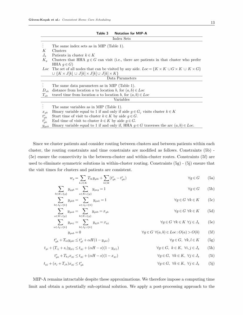
index sets, data parameters, and the variables are explained in Table 3.
The objective function remains the same as in MIP. Note, however, that the routing variable
ygab is defined on different arcs. For the Loc set defined in Table 3, the objective function is as
follows:
min∑
g∈G,(a,b)∈Loc
cTygabDab +∑f∈F
cFγf +∑p∈P
cPwp +∑f∈F
cOFOf +∑p∈P
cOP θp +∑j∈J
λpPj
In addition to the constraints of MIP model ((1a) - (1p)), we add the following constraints (4a)
- (4c) that are used to define the cluster-aide assignment variables and the visit times for the
clusters.
xgj ≤ xgk ≤∑j∈Jk
xgj ∀g ∈G ∀k ∈K ∀j ∈ Jk (4a)
0≤ tsgk ≤ (αH − s)xgk ∀g ∈G, ∀k ∈K (4b)
tegk = tsgk +( ∑
i,j∈Jk∪{k}
(Tij + sj)ygij +∑j∈Jk
Tjkygjk
)∀g ∈G, ∀k ∈K (4c)
xgk ∈ {0,1} ∀g ∈G ∀j ∈ J ∀k ∈K (4d)
Guven-Kocak et al.: Consistent Home Care Scheduling13
Table 3 Notation for MIP-A
Index Sets... The same index sets as in MIP (Table 1).K ClustersJk Patients in cluster k ∈KKg Clusters that HHA g ∈G can visit (i.e., there are patients in that cluster who prefer
HHA g ∈G)Loc The set of all nodes that can be visited by any aide. Loc= {K ×K ∪G×K ∪ K ×G}
∪ {K × J [k] ∪ J [k]× J [k]∪ J [k]×K}Data Parameters
... The same data parameters as in MIP (Table 1).Dab distance from location a to location b, for (a, b)∈LocTab travel time from location a to location b, for (a, b)∈Loc
Variables... The same variables as in MIP (Table 1).xgk Binary variable equal to 1 if and only if aide g ∈Gj visits cluster k ∈Ktsgk Start time of visit to cluster k ∈K by aide g ∈G.tegk End time of visit to cluster k ∈K by aide g ∈G.ygab Binary variable equal to 1 if and only if, HHA g ∈G traverses the arc (a, b)∈Loc.
Since we cluster patients and consider routing between clusters and between patients within each
cluster, the routing constraints and time constraints are modified as follows. Constraints (5b) -
(5e) ensure the connectivity in the between-cluster and within-cluster routes. Constraints (5f) are
used to eliminate symmetric solutions in within-cluster routing. Constraints (5g) - (5j) ensure that
the visit times for clusters and patients are consistent.
wg =∑k,l∈K
Tlkyglk +∑k∈K
(tegk− tsgk) ∀g ∈G (5a)∑b∈K∪{g}
yggb =∑
a∈K∪{g}
ygag = 1 ∀g ∈G (5b)∑b∈Jk∪{k}
ygkb =∑
a∈Jk∪{k}
ygak = 1 ∀g ∈G ∀k ∈K (5c)∑a∈K∪{g}
ygak =∑
b∈K∪{g}
ygkb = xgk ∀g ∈G ∀k ∈K (5d)∑a∈Jk∪{k}
ygaj =∑
b∈Jk∪{k}
ygjb = xgj ∀g ∈G ∀k ∈K ∀j ∈ Jk (5e)
ygab = 0 ∀g ∈G ∀(a, b)∈Loc :O(a)>O(b) (5f)
tegk +Tklygkl ≤ tsgl +αH(1− ygkl) ∀g ∈G, ∀k, l ∈K (5g)
tgi + (Tij + si)ygij ≤ tgj + (αH − s)(1− ygij) ∀g ∈G, k ∈K, ∀i, j ∈ Jk (5h)
tsgk +Tkjxgj ≤ tgj + (αH − s)(1−xgj) ∀g ∈G, ∀k ∈K, ∀j ∈ Jk (5i)
tgj + (sj +Tjk)xgj ≤ tegk ∀g ∈G, ∀k ∈K, ∀j ∈ Jk (5j)
MIP-A remains intractable despite these approximations. We therefore impose a computing time
limit and obtain a potentially sub-optimal solution. We apply a post-processing approach to the

Guven-Kocak et al.: Consistent Home Care Scheduling14
solution obtained using MIP-A to arrange the schedule and minimize costs. We obtain the HHA-
patient assignment information from the MIP-A solution and solve a TSP to re-create the routes
for each HHA. Since the number of patients in an HHA’s route is limited, solving this TSP can be
achieved efficiently. In other problem settings, where routes may be larger, a TSP heuristic may
be utilized. In addition to further minimizing costs, this post-processing step also supports more
accurate comparisons among different schedules by eliminating any idle times in the schedules and
revealing the actual costs.
MIP-A is modified to obtain an approximate MIP model for the Con-HHCRSP, which we refer
to as Con-MIP-A. The modifications are the same as explained in section 3.2. In other words,
we add index set, data parameters, and variables to the model as described in Table 2. The
objective function is modified to incorporate the consistency preference as in (2) and the consistency
constraints (3a) and (3b) are added to MIP-A.
4.2. Petal Based Heuristic for HHCRSP (PH)
The Petal Heuristic was first proposed by Foster and Ryan (1976) to address the vehicle scheduling
problem. This solution approach involves two stages. In the first stage, a set of possible “good”
routes is created. In the second stage, the assignment of the routes is made by solving a set
partitioning problem. This approach is appropriate for our problem setting, as the number of daily
visits is limited. In our instances, a single HHA can visit at most five patients each day so routing is
simplified once the visit assignment is determined. We therefore develop a variant of this heuristic,
denoted PH, to address HHCRSP.
We first develop an algorithm to create a “good” set of clusters. Here, “good” clusters refer
to groups of patients who are highly likely to be visited by the same aide (due to the patients’
similarities with respect to location and preferences). When creating the clusters of patients, we
exclude infeasible sets, i.e., sets of patients who cannot be visited by the same HHA on a single day
within regular working hours. Algorithm 1 is used to generate a “good” set of clusters of patients
who can be visited by the same HHA on a single day. Here, we aim to group patients into clusters
without considering the order in which they are visited. The routes are created after the clusters
are formed.
The pseudo-code of our cluster generation algorithm is written in Algorithm 1. Steps 1-6 are used
to generate all possible singletons and pairs of patients; steps 7-19 are used to generate clusters of
3, 4, and 5 patients. Note that in our instance an HHA may visit at most five patients each day,
so we limit the size of the clusters to equal five. In other instances, the size of the clusters may be
set to a larger value in step 8 of the algorithm. We repeat the second part of the algorithm (steps
8-19) twice for modified and unmodified distance matrices. The unmodified distance matrix is a

Guven-Kocak et al.: Consistent Home Care Scheduling15
Algorithm 1: Algorithm for Cluster Generation
1 Initial Solution: C = ∅ (set of clusters), Ignore=NULL ;
2 (Create all possible clusters of one and two patients) ;
3 forall i∈ Patients do4 C =C ∪{(i)}∪ ∅ /; forall j ∈ Patients \{i} do5 if {(i, j)} /∈C then6 C =C ∪{i, j}
7 for modified and unmodified distance matrices do8 forall x∈ [3,4,5] do9 (Create clusters of x patients) ;
10 forall i1 ∈ Patients do11 Ignore=i1 ;
12 while There are less than Cx clusters including patient i1 do13 while The size of the cluster is less than x (|c|<x) do14 Use Nearest Insertion to find c= {i2, ..., ix} ∈ Patients \ Ignore. ;
15 Ignore=Ignore ∪{i2, ..., ix} ;
16 if {i1, i2, ..., ix} /∈C is a feasible route then17 C =C ∪{i1, i2, ..., ix}18 c= {i1, i2, ..., ix−j}
19 (Keep the first j elements of the cluster the same, and create more clusters,
where j ∈ {2, ..., x− 1}. Do this twice for each j, starting with j = x− 1.)
location based distance matrix obtained from Google Maps. We modify this distance matrix based
on patient preferences. Namely, for each pair of patients, we add the preference cost to the distance
between them if all of their preferred aides are different. In this way, we aim to cluster patients
with similar aide preferences. This also introduces more flexibility in options when we assign the
clusters to HHAs using a set partitioning formulation.
After the clusters are created, we calculate the “assignment costs” of each HHA to each cluster.
The assignment cost includes travel cost (total distance within the cluster plus distance to / from
HHA’s home from / to the nearest patient in the cluster), overtime cost, idle time cost for FT
HHA, hourly labor cost for PT HHA, and the penalty for any preference violations (penalty for
one preference violation, multiplied by the number of patients in the corresponding cluster who
do not prefer that HHA). The main steps involved in creating the routes and calculating the costs
of each cluster-HHA assignment are: (i) For each cluster, create a route using TSP and calculate
the minimum travel distance and the travel time for the route. (ii) If the total travel time for the
route exceeds the daily time limit then delete this route. Otherwise, add this route to the set of

Guven-Kocak et al.: Consistent Home Care Scheduling16
“good” routes. (iii) For each HHA, record the cost of visiting each route if the total travel time of
the route is within the daily time limits.
The assignment cost for each aide and each route includes travel, labor (work time and idle
time), overtime, and preference penalty costs. As mentioned above, we first create a TSP tour
with the set of patients within each cluster generated with Algorithm 1. Next, using the cheapest
insertion algorithm, we create a route for each aide by determining the first and last patients to
visit on the TSP tour of patients, based on the home locations of the aide and the patients. Once
all possible routes are created, we calculate the total travel distance within each route by summing
up the travel distances; we compute total time by summing travel times and service times. The
travel cost is obtained by multiplying total travel distance by the unit travel cost. The labor cost
for part-time HHAs is calculated by multiplying the hourly PT labor cost by the total number of
hours an aide works each day; the labor cost for full-time HHAs is calculated by multiplying the
hourly FT labor cost with the idle time spent by a FT aide (i.e., difference between the regular
working hours and the actual time an aide works on a day). Overtime cost for part-time HHAs is
a one-time cost added if the total number of hours worked is above a certain limit; overtime cost
for full-time HHAs is calculated by multiplying the hourly FT labor overtime cost with the total
number of hours worked above the regular daily hours. Finally, preference cost is calculated by
multiplying the preference penalty unit cost by the total number of patients within a cluster who
do not prefer the aide visiting that cluster.
After the assignment costs are calculated, a variant of a Set Partitioning Problem is solved to
assign the routes to aides such that the cost of the resulting schedule is minimized. The notation
used in the set partitioning model is explained in Table 9 in Appendix A. Once the route-aide
assignments are made, the schedules are created by calculating the arrival time for each patient in
the pre-determined routes.
4.3. Petal Based Heuristic for Con-HHCRSP (Con-PH)
We modify the petal based heuristic proposed for HHCRSP (PH) to solve Con-HHCRSP. We
denote this modified version of the petal heuristic as Con-PH. The location-based distance matrix is
modified based on the patient preferences as explained in Section 4.2. To account for the deviations
from the previous schedule, we modify the distance matrix as follows. For each pair of patients, we
add the deviation cost to the distance between them if they were visited by different aides in the
previous assignment. This way, we aim to cluster patients who have been visited by the same aide
in the previous assignment.
This modification to the distance matrix helps to create clusters based on location, preferences,
and previous assignments. However, it is still insufficient to fully recover the previous schedule.
Guven-Kocak et al.: Consistent Home Care Scheduling17
That is, we cannot guarantee that the clusters generated using these modified and unmodified
distance matrices will provide an option of retaining the previous schedule. Therefore, in addition
to the clusters generated by Algorithm 1, we generate clusters that focus on consistency using
the regret-based repair operators as follows. First, we take the routes of the previous schedule as
an initial set of clusters and remove patients who are not in the current data set. Then, we use
the regret operator to insert each new patient into an aide’s daily route by considering the regret
cost of postponing an insertion to later iterations (Potvin and Rousseau (1993)). In this way, we
generate a route for each aide that retains all of the previous assignments. We randomize the order
in the set of new patients and create more clusters using the regret operator.
The regret operator calculates the cost for several insertion positions for each patient and finds
the difference between the cost of the best insertion position and the cost of the alternative insertion
positions as follows:
∆i =
min(r,m)∑k=2
(cki − c1i ).
Here, r is the regret operator parameter that refers to the number of routes to be considered in
comparison and m is the total number of possible routes; cki refers to the kth cheapest insertion
cost for patient i. Based on this cost calculation, the regret operator inserts the patient with the
largest difference between the cost of the best insertion position and alternative insertion positions.
Namely, i∗ = arg maxi∈I\{i}∆i is inserted to its cheapest position. The process is repeated until all
new patients are inserted. In our implementation, we set the regret parameter equal to half the
size of the new patients.
We incorporate the inconsistency penalty into the cost. In addition to the cost items explained
in Section 4.2, we add inconsistency cost to the overall assignment cost between each cluster and
aide. For a given cluster-aide pair, if there are patients in the cluster who were visited by another
aide in the previous schedule, then the unit cost of inconsistency is multiplied by the number of
patients in this situation and added to the assignment cost. This encourages the set partitioning
model solution to be consistent with the previous schedule.
4.4. Improvement Heuristics.
To improve the solutions we obtain via PH or MIP-A, we also develop fast and simple improve-
ment heuristics. Specifically, we implemented various swap heuristics. The single-swap heuristic
considers each patient in sequence and determines if there is an aide, other than the one currently
assigned, who can serve the patient at a lower cost. The double-swap heuristic considers patient
pairs and swaps their assignments if the resulting net cost is lower. The combined single and dou-
ble heuristic performs single-swap heuristic and double-swap heuristic in sequence. In all these
heuristics, improvement iteration is repeated until no more improvements can be made in the last

Guven-Kocak et al.: Consistent Home Care Scheduling18
iteration. Moreover, note that the swapping decisions are evaluated in terms of the assignments
rather than the actual locations on the routes. Therefore, when an assignment is under evaluation,
the new routes are created by solving TSP and then the net costs are calculated. For example, in
the double-swap heuristic, when a swapping decision of patient a and b is evaluated, the new routes
of the aide who originally visited patient a and the aide who originally visited patient b are found
by solving TSP and the optimum costs of the newly formed routes are calculated accordingly. If
the net cost is negative, then the assignments of the patients are swapped and the new routes of
the aides are set to the TSP route that was found during the evaluation step. This way, we always
keep the optimum routes for aides, given their daily assignments.
The algorithms of our versions of swap heuristics, as well as the results of the computational
experiments, can be found in Appendix A.2. Based on our experiments, we found the combined
single and double swap heuristic to be most effective. We therefore chose to use this heuristic in
our computational experiments.
5. Computational Experiments.
In this section, we describe the results of a computational study aimed at comparing the perfor-
mances of the methods described in Section 4 and exploring the effect of the continuity of care
requirement on the scheduling decisions. For the purposes of this study, we obtained data from a
real-world home health care agency operating in the United States. The experiments have been
performed on an Intel(R) Core(TM) Processor i7-4785T (CPU 2.20 GHz) with 16 GB of memory,
using the solver Gurobi 7.0.1 with a maximum time limit of 12 hours for mixed integer programming
models. In the results, the computational times are expressed in seconds of CPU time.
5.1. Data
We address a real-world home health care routing and scheduling problem faced by a hospice agency
that operates in the United States. This hospice agency has operated for more than two decades
and has branches in more than 20 states. We collaborated with one of the agency’s branches and
used their data as the basis for our computational experiments. This dataset, associated with one
city-branch of the agency, contains information on 98 patients and 24 aides. All data has been
masked in accordance with HIPAA requirements. The approximate locations of the patients and
the aides are shown on the map in Figure 1.
Per government eligibility requirements, a patient is deemed hospice-eligible if he has an expected
remaining lifetime of six months or less if his disease were to run its normal course. The objective
of hospice care is not to provide curative care, but rather, to increase patient quality of life and
provide the patient with end-of-life comfort and reduced pain. To increase patient and family
comfort during this final phase in life, the agency asks the patients if they have any preferences
Guven-Kocak et al.: Consistent Home Care Scheduling19
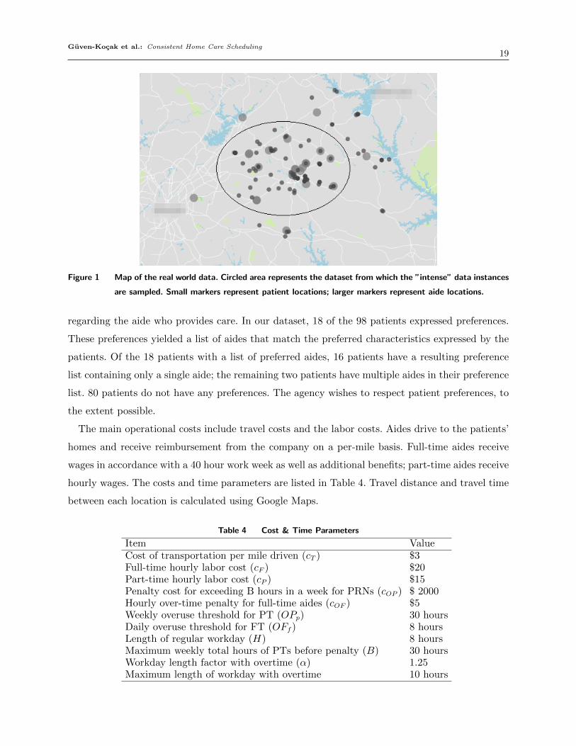
Figure 1 Map of the real world data. Circled area represents the dataset from which the ”intense” data instances
are sampled. Small markers represent patient locations; larger markers represent aide locations.
regarding the aide who provides care. In our dataset, 18 of the 98 patients expressed preferences.
These preferences yielded a list of aides that match the preferred characteristics expressed by the
patients. Of the 18 patients with a list of preferred aides, 16 patients have a resulting preference
list containing only a single aide; the remaining two patients have multiple aides in their preference
list. 80 patients do not have any preferences. The agency wishes to respect patient preferences, to
the extent possible.
The main operational costs include travel costs and the labor costs. Aides drive to the patients’
homes and receive reimbursement from the company on a per-mile basis. Full-time aides receive
wages in accordance with a 40 hour work week as well as additional benefits; part-time aides receive
hourly wages. The costs and time parameters are listed in Table 4. Travel distance and travel time
between each location is calculated using Google Maps.
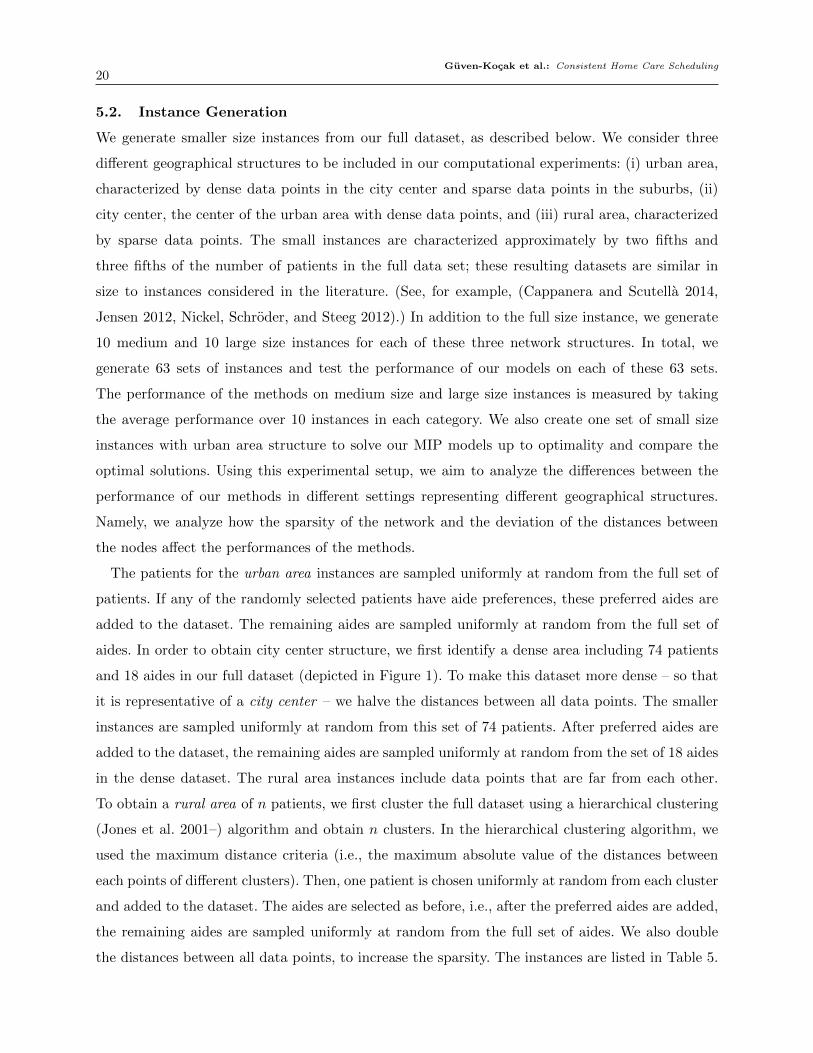
Table 4 Cost & Time Parameters
Item ValueCost of transportation per mile driven (cT ) $3Full-time hourly labor cost (cF ) $20Part-time hourly labor cost (cP ) $15Penalty cost for exceeding B hours in a week for PRNs (cOP ) $ 2000Hourly over-time penalty for full-time aides (cOF ) $5Weekly overuse threshold for PT (OPp) 30 hoursDaily overuse threshold for FT (OFf ) 8 hoursLength of regular workday (H) 8 hoursMaximum weekly total hours of PTs before penalty (B) 30 hoursWorkday length factor with overtime (α) 1.25Maximum length of workday with overtime 10 hours
Guven-Kocak et al.: Consistent Home Care Scheduling20
5.2. Instance Generation
We generate smaller size instances from our full dataset, as described below. We consider three
different geographical structures to be included in our computational experiments: (i) urban area,
characterized by dense data points in the city center and sparse data points in the suburbs, (ii)
city center, the center of the urban area with dense data points, and (iii) rural area, characterized
by sparse data points. The small instances are characterized approximately by two fifths and
three fifths of the number of patients in the full data set; these resulting datasets are similar in
size to instances considered in the literature. (See, for example, (Cappanera and Scutella 2014,
Jensen 2012, Nickel, Schroder, and Steeg 2012).) In addition to the full size instance, we generate
10 medium and 10 large size instances for each of these three network structures. In total, we
generate 63 sets of instances and test the performance of our models on each of these 63 sets.
The performance of the methods on medium size and large size instances is measured by taking
the average performance over 10 instances in each category. We also create one set of small size
instances with urban area structure to solve our MIP models up to optimality and compare the
optimal solutions. Using this experimental setup, we aim to analyze the differences between the
performance of our methods in different settings representing different geographical structures.
Namely, we analyze how the sparsity of the network and the deviation of the distances between
the nodes affect the performances of the methods.
The patients for the urban area instances are sampled uniformly at random from the full set of
patients. If any of the randomly selected patients have aide preferences, these preferred aides are
added to the dataset. The remaining aides are sampled uniformly at random from the full set of
aides. In order to obtain city center structure, we first identify a dense area including 74 patients
and 18 aides in our full dataset (depicted in Figure 1). To make this dataset more dense – so that
it is representative of a city center – we halve the distances between all data points. The smaller
instances are sampled uniformly at random from this set of 74 patients. After preferred aides are
added to the dataset, the remaining aides are sampled uniformly at random from the set of 18 aides
in the dense dataset. The rural area instances include data points that are far from each other.
To obtain a rural area of n patients, we first cluster the full dataset using a hierarchical clustering
(Jones et al. 2001–) algorithm and obtain n clusters. In the hierarchical clustering algorithm, we
used the maximum distance criteria (i.e., the maximum absolute value of the distances between
each points of different clusters). Then, one patient is chosen uniformly at random from each cluster
and added to the dataset. The aides are selected as before, i.e., after the preferred aides are added,
the remaining aides are sampled uniformly at random from the full set of aides. We also double
the distances between all data points, to increase the sparsity. The instances are listed in Table 5.
Guven-Kocak et al.: Consistent Home Care Scheduling21
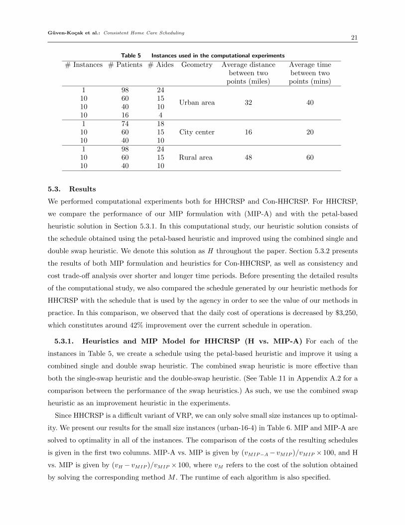
Table 5 Instances used in the computational experiments
# Instances # Patients # Aides Geometry Average distancebetween two
points (miles)
Average timebetween twopoints (mins)
1 98 24
Urban area 32 4010 60 1510 40 1010 16 41 74 18
City center 16 2010 60 1510 40 101 98 24
Rural area 48 6010 60 1510 40 10
5.3. Results
We performed computational experiments both for HHCRSP and Con-HHCRSP. For HHCRSP,
we compare the performance of our MIP formulation with (MIP-A) and with the petal-based
heuristic solution in Section 5.3.1. In this computational study, our heuristic solution consists of
the schedule obtained using the petal-based heuristic and improved using the combined single and
double swap heuristic. We denote this solution as H throughout the paper. Section 5.3.2 presents
the results of both MIP formulation and heuristics for Con-HHCRSP, as well as consistency and
cost trade-off analysis over shorter and longer time periods. Before presenting the detailed results
of the computational study, we also compared the schedule generated by our heuristic methods for
HHCRSP with the schedule that is used by the agency in order to see the value of our methods in
practice. In this comparison, we observed that the daily cost of operations is decreased by $3,250,
which constitutes around 42% improvement over the current schedule in operation.
5.3.1. Heuristics and MIP Model for HHCRSP (H vs. MIP-A) For each of the
instances in Table 5, we create a schedule using the petal-based heuristic and improve it using a
combined single and double swap heuristic. The combined swap heuristic is more effective than
both the single-swap heuristic and the double-swap heuristic. (See Table 11 in Appendix A.2 for a
comparison between the performance of the swap heuristics.) As such, we use the combined swap
heuristic as an improvement heuristic in the experiments.
Since HHCRSP is a difficult variant of VRP, we can only solve small size instances up to optimal-
ity. We present our results for the small size instances (urban-16-4) in Table 6. MIP and MIP-A are
solved to optimality in all of the instances. The comparison of the costs of the resulting schedules
is given in the first two columns. MIP-A vs. MIP is given by (vMIP−A− vMIP )/vMIP × 100, and H
vs. MIP is given by (vH − vMIP )/vMIP × 100, where vM refers to the cost of the solution obtained
by solving the corresponding method M . The runtime of each algorithm is also specified.
Guven-Kocak et al.: Consistent Home Care Scheduling22
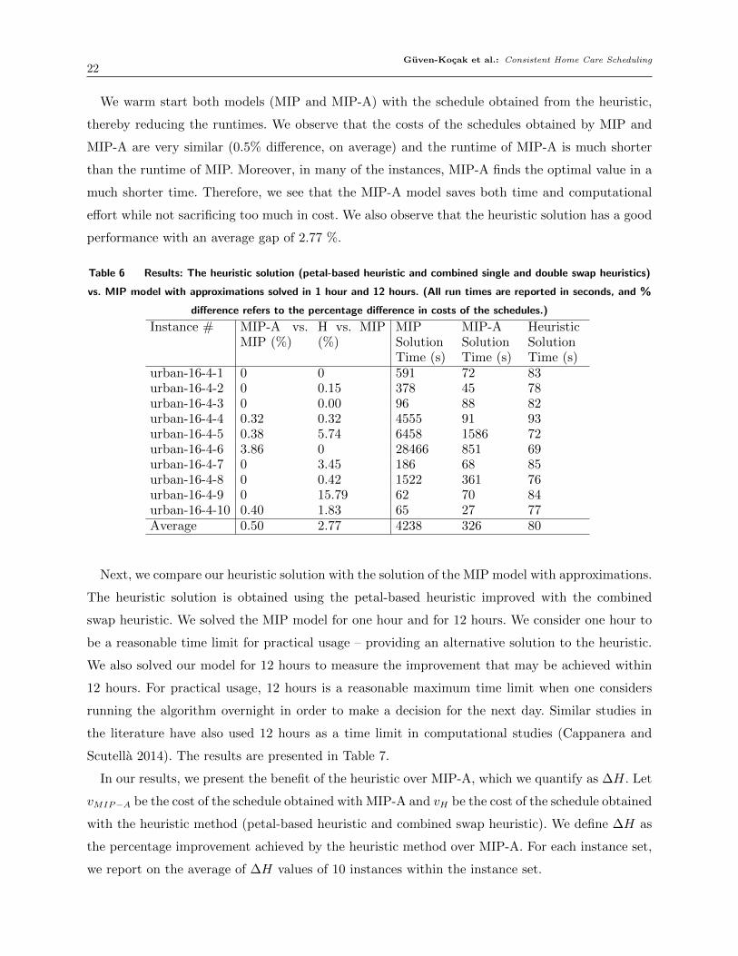
We warm start both models (MIP and MIP-A) with the schedule obtained from the heuristic,
thereby reducing the runtimes. We observe that the costs of the schedules obtained by MIP and
MIP-A are very similar (0.5% difference, on average) and the runtime of MIP-A is much shorter
than the runtime of MIP. Moreover, in many of the instances, MIP-A finds the optimal value in a
much shorter time. Therefore, we see that the MIP-A model saves both time and computational
effort while not sacrificing too much in cost. We also observe that the heuristic solution has a good
performance with an average gap of 2.77 %.
Table 6 Results: The heuristic solution (petal-based heuristic and combined single and double swap heuristics)
vs. MIP model with approximations solved in 1 hour and 12 hours. (All run times are reported in seconds, and %
difference refers to the percentage difference in costs of the schedules.)
Instance # MIP-A vs.MIP (%)
H vs. MIP(%)
MIPSolutionTime (s)
MIP-ASolutionTime (s)
HeuristicSolutionTime (s)
urban-16-4-1 0 0 591 72 83urban-16-4-2 0 0.15 378 45 78urban-16-4-3 0 0.00 96 88 82urban-16-4-4 0.32 0.32 4555 91 93urban-16-4-5 0.38 5.74 6458 1586 72urban-16-4-6 3.86 0 28466 851 69urban-16-4-7 0 3.45 186 68 85urban-16-4-8 0 0.42 1522 361 76urban-16-4-9 0 15.79 62 70 84urban-16-4-10 0.40 1.83 65 27 77Average 0.50 2.77 4238 326 80
Next, we compare our heuristic solution with the solution of the MIP model with approximations.
The heuristic solution is obtained using the petal-based heuristic improved with the combined
swap heuristic. We solved the MIP model for one hour and for 12 hours. We consider one hour to
be a reasonable time limit for practical usage – providing an alternative solution to the heuristic.
We also solved our model for 12 hours to measure the improvement that may be achieved within
12 hours. For practical usage, 12 hours is a reasonable maximum time limit when one considers
running the algorithm overnight in order to make a decision for the next day. Similar studies in
the literature have also used 12 hours as a time limit in computational studies (Cappanera and
Scutella 2014). The results are presented in Table 7.
In our results, we present the benefit of the heuristic over MIP-A, which we quantify as ∆H. Let
vMIP−A be the cost of the schedule obtained with MIP-A and vH be the cost of the schedule obtained
with the heuristic method (petal-based heuristic and combined swap heuristic). We define ∆H as
the percentage improvement achieved by the heuristic method over MIP-A. For each instance set,
we report on the average of ∆H values of 10 instances within the instance set.
Guven-Kocak et al.: Consistent Home Care Scheduling23
∆H =vMIP−A− vHvMIP−A
× 100
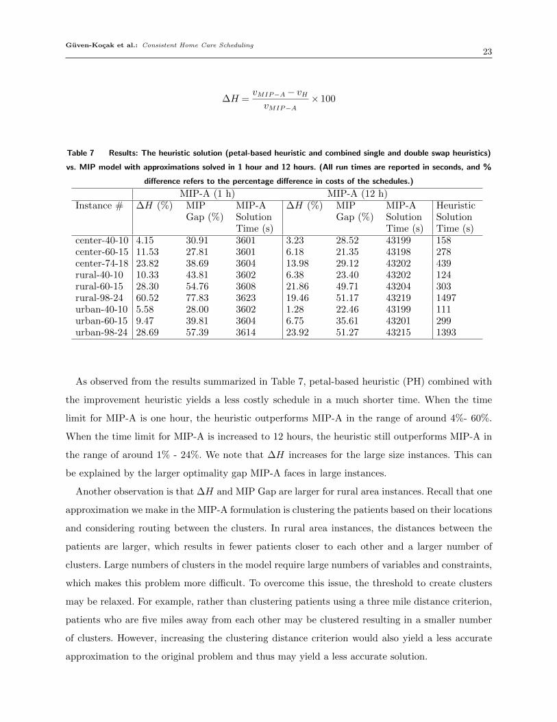
Table 7 Results: The heuristic solution (petal-based heuristic and combined single and double swap heuristics)
vs. MIP model with approximations solved in 1 hour and 12 hours. (All run times are reported in seconds, and %
difference refers to the percentage difference in costs of the schedules.)
MIP-A (1 h) MIP-A (12 h)Instance # ∆H (%) MIP
Gap (%)MIP-ASolutionTime (s)
∆H (%) MIPGap (%)
MIP-ASolutionTime (s)
HeuristicSolutionTime (s)
center-40-10 4.15 30.91 3601 3.23 28.52 43199 158center-60-15 11.53 27.81 3601 6.18 21.35 43198 278center-74-18 23.82 38.69 3604 13.98 29.12 43202 439rural-40-10 10.33 43.81 3602 6.38 23.40 43202 124rural-60-15 28.30 54.76 3608 21.86 49.71 43204 303rural-98-24 60.52 77.83 3623 19.46 51.17 43219 1497urban-40-10 5.58 28.00 3602 1.28 22.46 43199 111urban-60-15 9.47 39.81 3604 6.75 35.61 43201 299urban-98-24 28.69 57.39 3614 23.92 51.27 43215 1393
As observed from the results summarized in Table 7, petal-based heuristic (PH) combined with
the improvement heuristic yields a less costly schedule in a much shorter time. When the time
limit for MIP-A is one hour, the heuristic outperforms MIP-A in the range of around 4%- 60%.
When the time limit for MIP-A is increased to 12 hours, the heuristic still outperforms MIP-A in
the range of around 1% - 24%. We note that ∆H increases for the large size instances. This can
be explained by the larger optimality gap MIP-A faces in large instances.
Another observation is that ∆H and MIP Gap are larger for rural area instances. Recall that one
approximation we make in the MIP-A formulation is clustering the patients based on their locations
and considering routing between the clusters. In rural area instances, the distances between the
patients are larger, which results in fewer patients closer to each other and a larger number of
clusters. Large numbers of clusters in the model require large numbers of variables and constraints,
which makes this problem more difficult. To overcome this issue, the threshold to create clusters
may be relaxed. For example, rather than clustering patients using a three mile distance criterion,
patients who are five miles away from each other may be clustered resulting in a smaller number
of clusters. However, increasing the clustering distance criterion would also yield a less accurate
approximation to the original problem and thus may yield a less accurate solution.
Guven-Kocak et al.: Consistent Home Care Scheduling24
5.3.2. Heuristics and MIP Model for Con-HHCRSP (Con-H vs. Con-MIP-A) In
this section, we present our results for Con-HHCRSP methods. For this analysis, we generate an
updated set of instances from our original instances (presented in Table 5). The updated dataset
represents the data of the next period of the original dataset. To generate the updated datasets, we
assume that 20% of the patients in the original dataset change in the next period while the set of
aides and data parameters in Table 4 remain the same. We sample uniformly at random from the
existing set of patients to identify the patients that leave the dataset. The patients added to the
dataset are sampled uniformly at random from the set of patients in the full dataset; patients are
only added to the updated instance set if one of their preferred aides is in the existing set of aides.
The total number of patients does not change when we update the instance set. We first update the
schedules based on the updated dataset, using both Con-H and Con-MIP-A, and compare the cost
of the schedules and the solution times of both methods. We test the methods on 60 sets of medium
and large instances having different network structures, as explained in Section 5.2. Further, we
present our analysis of the impact of the inconsistency penalty on the cost of the schedule; this
analysis sheds insight on the cost and consistency trade-off in this problem. Finally, we analyze
the long-term cost effect of the consistency policy on the cost, by generating 50 updated dataset
instances and updating the schedules over 50 periods. The results are presented below.
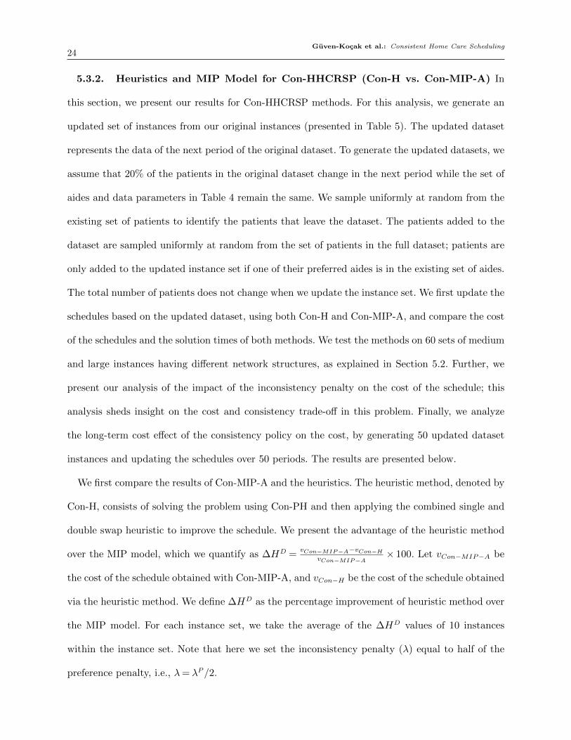
We first compare the results of Con-MIP-A and the heuristics. The heuristic method, denoted by
Con-H, consists of solving the problem using Con-PH and then applying the combined single and
double swap heuristic to improve the schedule. We present the advantage of the heuristic method
over the MIP model, which we quantify as ∆HD =vCon−MIP−A−vCon−H
vCon−MIP−A× 100. Let vCon−MIP−A be
the cost of the schedule obtained with Con-MIP-A, and vCon−H be the cost of the schedule obtained
via the heuristic method. We define ∆HD as the percentage improvement of heuristic method over
the MIP model. For each instance set, we take the average of the ∆HD values of 10 instances
within the instance set. Note that here we set the inconsistency penalty (λ) equal to half of the
preference penalty, i.e., λ= λP/2.
Guven-Kocak et al.: Consistent Home Care Scheduling25
Table 8 Results: The heuristic Con-H (petal-based heuristic and combined single and double swap heuristics)
vs. Con-MIP-A solved in 1 hour and 12 hours. (All run times are reported in seconds, and % difference refers to
the percentage difference in costs of the schedules.)
Con-MIP-A (1 h) Con-MIP-A (12 h)Instance # ∆HD (%) MIP
Gap (%)Con-MIP-ASolutionTime (s)
∆HD (%) MIPGap (%)
Con-MIP-ASolutionTime (s)
HeuristicSolutionTime (s)
center-40-10 0.52 6.66 1326 0.52 6.26 9248 246center-60-15 0.82 3.24 2614 0.82 1.86 21066 638rural-40-10 6.15 13.90 3604 6.13 9.87 43202 269rural-60-15 3.75 13.98 3609 3.47 10.36 43204 722urban-40-10 -0.23 3.58 2206 -0.32 1.77 11360 248urban-60-15 0.33 13.17 3605 0.29 10.36 43203 690
Table 8 presents the comparison between the heuristic (Con-H) and the MIP formulation (Con-
MIP-A). We observe that the heuristic outperforms the MIP formulation in all instances except
urban-40-10. In the case of urban-40-10, after one hour (after 12 hours) Con-MIP-A produces a
solution that is 0.23% (0.32%) less costly than the heuristic solution. In other words, a difference
of less than 0.35% in the cost is achieved while there are significant savings in the solution time
and computational effort. The same is not observed for urban-60-15 due to the large MIP gap of
Con-MIP-A within a given time limit. One reason for this observation could be the fact that there
is a large deviation in the distances between any two points. As such, swapping two nodes in the
resulting routes may result in a large cost difference.
Next, we analyze how the consistency and cost are affected by the use of different inconsistency
penalties in Con-PH. Here, consistency is measured by the number of patients assigned to a different
aide in the new schedule as a percentage of the total number of patients who are included both in
the previous and the new datasets. As explained earlier, we assume that 20% of the patients in the
original dataset are different than the new dataset. The inconsistency penalty (λ) is obtained by
multiplying the inconsistency penalty coefficient (cλ) and the penalty for the preference violation
(λP ), i.e. λ= cλλP . When we set cλ = 0, we obtain a schedule without consistency restriction. We
compare the cost of the schedules we obtain with positive cλ values to the cost of the schedule we
obtain with cλ = 0 as follows:
∆Cλ =vλCon−PH − v0Con−PH
v0Con−PH× 100
For each instance set, we take the average of the ∆Cλ values of 10 instances within the instance
set. The detailed results of this analysis are presented in Table 12. We present a summary of
the results in Figure 2, which depicts average results over all instances. As observed, both the
Guven-Kocak et al.: Consistent Home Care Scheduling26
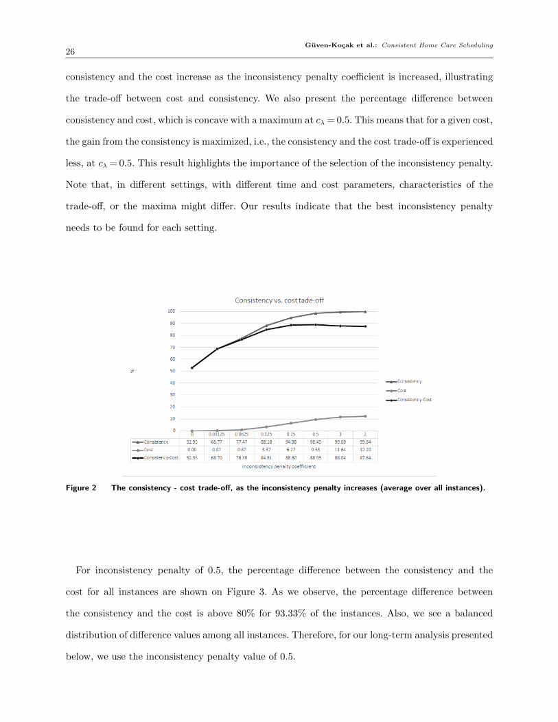
consistency and the cost increase as the inconsistency penalty coefficient is increased, illustrating
the trade-off between cost and consistency. We also present the percentage difference between
consistency and cost, which is concave with a maximum at cλ = 0.5. This means that for a given cost,
the gain from the consistency is maximized, i.e., the consistency and the cost trade-off is experienced
less, at cλ = 0.5. This result highlights the importance of the selection of the inconsistency penalty.
Note that, in different settings, with different time and cost parameters, characteristics of the
trade-off, or the maxima might differ. Our results indicate that the best inconsistency penalty
needs to be found for each setting.
Figure 2 The consistency - cost trade-off, as the inconsistency penalty increases (average over all instances).
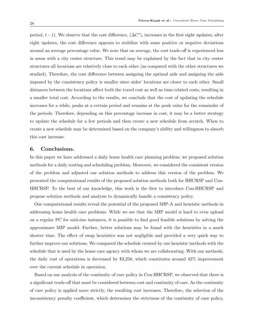
For inconsistency penalty of 0.5, the percentage difference between the consistency and the
cost for all instances are shown on Figure 3. As we observe, the percentage difference between
the consistency and the cost is above 80% for 93.33% of the instances. Also, we see a balanced
distribution of difference values among all instances. Therefore, for our long-term analysis presented
below, we use the inconsistency penalty value of 0.5.
Guven-Kocak et al.: Consistent Home Care Scheduling27
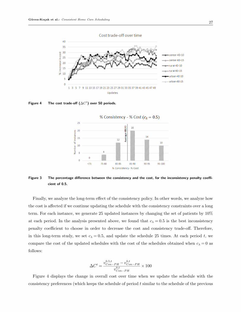
Figure 4 The cost trade-off (∆Ct) over 50 periods.
Figure 3 The percentage difference between the consistency and the cost, for the inconsistency penalty coeffi-
cient of 0.5.
Finally, we analyze the long-term effect of the consistency policy. In other words, we analyze how
the cost is affected if we continue updating the schedule with the consistency constraints over a long
term. For each instance, we generate 25 updated instances by changing the set of patients by 10%
at each period. In the analysis presented above, we found that cλ = 0.5 is the best inconsistency
penalty coefficient to choose in order to decrease the cost and consistency trade-off. Therefore,
in this long-term study, we set cλ = 0.5, and update the schedule 25 times. At each period t, we
compare the cost of the updated schedules with the cost of the schedules obtained when cλ = 0 as
follows:
∆Ct =v0.5,tCon−PH − v
0,tCon−PH
v0,tCon−PH× 100
Figure 4 displays the change in overall cost over time when we update the schedule with the
consistency preferences (which keeps the schedule of period t similar to the schedule of the previous
Guven-Kocak et al.: Consistent Home Care Scheduling28
period, t−1). We observe that the cost difference, (∆Ct), increases in the first eight updates; after
eight updates, the cost difference appears to stabilize with some positive or negative deviations
around an average percentage value. We note that on average, the cost trade-off is experienced less
in areas with a city center structure. This trend may be explained by the fact that in city center
structures all locations are relatively close to each other (as compared with the other structures we
studied). Therefore, the cost difference between assigning the optimal aide and assigning the aide
imposed by the consistency policy is smaller since aides’ locations are closer to each other. Small
distances between the locations affect both the travel cost as well as time-related costs, resulting in
a smaller total cost. According to the results, we conclude that the cost of updating the schedule
increases for a while, peaks at a certain period and remains at the peak value for the remainder of
the periods. Therefore, depending on this percentage increase in cost, it may be a better strategy
to update the schedule for a few periods and then create a new schedule from scratch. When to
create a new schedule may be determined based on the company’s ability and willingness to absorb
this cost increase.
6. Conclusions.
In this paper we have addressed a daily home health care planning problem; we proposed solution
methods for a daily routing and scheduling problem. Moreover, we considered the consistent version
of the problem and adjusted our solution methods to address this version of the problem. We
presented the computational results of the proposed solution methods both for HHCRSP and Con-
HHCRSP. To the best of our knowledge, this work is the first to introduce Con-HHCRSP and
propose solution methods and analysis to dynamically handle a consistency policy.
Our computational results reveal the potential of the proposed MIP-A and heuristic methods in
addressing home health care problems. While we see that the MIP model is hard to even upload
on a regular PC for mid-size instances, it is possible to find good feasible solutions by solving the
approximate MIP model. Further, better solutions may be found with the heuristics in a much
shorter time. The effect of swap heuristics was not negligible and provided a very quick way to
further improve our solutions. We compared the schedule created by our heuristic methods with the
schedule that is used by the home care agency with whom we are collaborating. With our methods,
the daily cost of operations is decreased by $3,250, which constitutes around 42% improvement
over the current schedule in operation.
Based on our analysis of the continuity of care policy in Con-HHCRSP, we observed that there is
a significant trade-off that must be considered between cost and continuity of care. As the continuity
of care policy is applied more strictly, the resulting cost increases. Therefore, the selection of the
inconsistency penalty coefficient, which determines the strictness of the continuity of care policy,
Guven-Kocak et al.: Consistent Home Care Scheduling29
is critical. Moreover, the effect of the continuity of care policy on the cost may grow large in the
long-term. Our long-term analysis revealed a rapidly increasing trend in the cost trade-off over
time in the first eight periods, and then a stabilized trend for the remainder of the periods. This
analysis should be used as a basis for deciding how many times to update the existing schedule
and when to solve it from scratch.
As a future research direction, the proposed solution methods can be extended for a weekly
planning problem. This can be achieved by converting a daily schedule to a weekly schedule using
a template-based approach or by developing a different solution method for the weekly problem.
Moreover, the methods may be extended to handle situations such as skilled nurses, time windows,
and interdependent visits.

Guven-Kocak et al.: Consistent Home Care Scheduling30
Appendix A: Models & Algorithms
A.1. Set Partitioning Model
Table 9 Notation for the Set Partitioning Model
Index SetsP PatientsA AidesC Clusters
Data Parameterswac The cost of assigning cluster c∈C to aide a∈A
Variablesxap Assigning patient p∈ P to aide a∈Axac Assigning cluster c∈C to aide a∈A
Table 10 The Set Partitioning Model
Index Sets
Objective: min∑
a∈A∑
c∈C wacxac
Constraints: s.t.∑a∈A
xap = 1∑c∈C
xac = 1∑a∈A
xac ≤ 1∑c3p
xac = xap ∀p∈ P ; ∀a∈A
xap, xac ∈ {0,1} ∀a∈A; ∀c∈C; ∀p∈ P
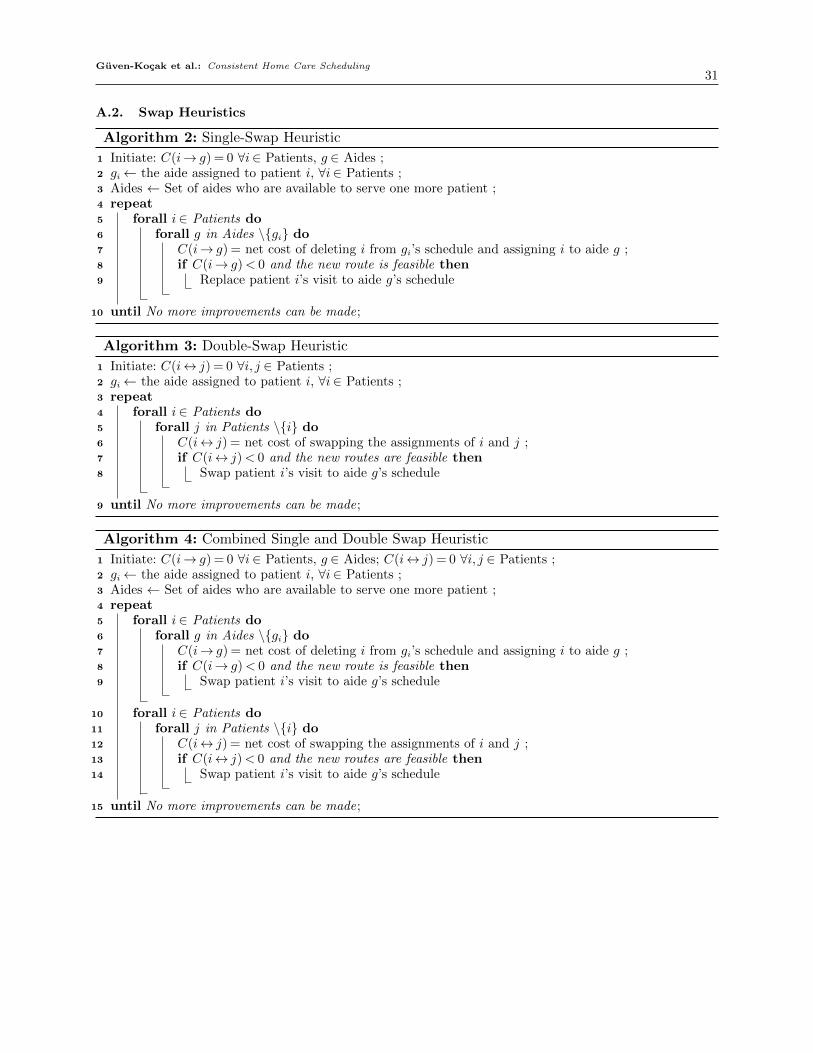
Guven-Kocak et al.: Consistent Home Care Scheduling31
A.2. Swap Heuristics
Algorithm 2: Single-Swap Heuristic
1 Initiate: C(i→ g) = 0 ∀i∈ Patients, g ∈ Aides ;2 gi← the aide assigned to patient i, ∀i∈ Patients ;3 Aides ← Set of aides who are available to serve one more patient ;4 repeat5 forall i∈ Patients do6 forall g in Aides \{gi} do7 C(i→ g) = net cost of deleting i from gi’s schedule and assigning i to aide g ;8 if C(i→ g)< 0 and the new route is feasible then9 Replace patient i’s visit to aide g’s schedule
10 until No more improvements can be made;
Algorithm 3: Double-Swap Heuristic
1 Initiate: C(i↔ j) = 0 ∀i, j ∈ Patients ;2 gi← the aide assigned to patient i, ∀i∈ Patients ;3 repeat4 forall i∈ Patients do5 forall j in Patients \{i} do6 C(i↔ j) = net cost of swapping the assignments of i and j ;7 if C(i↔ j)< 0 and the new routes are feasible then8 Swap patient i’s visit to aide g’s schedule
9 until No more improvements can be made;
Algorithm 4: Combined Single and Double Swap Heuristic
1 Initiate: C(i→ g) = 0 ∀i∈ Patients, g ∈ Aides; C(i↔ j) = 0 ∀i, j ∈ Patients ;2 gi← the aide assigned to patient i, ∀i∈ Patients ;3 Aides ← Set of aides who are available to serve one more patient ;4 repeat5 forall i∈ Patients do6 forall g in Aides \{gi} do7 C(i→ g) = net cost of deleting i from gi’s schedule and assigning i to aide g ;8 if C(i→ g)< 0 and the new route is feasible then9 Swap patient i’s visit to aide g’s schedule
10 forall i∈ Patients do11 forall j in Patients \{i} do12 C(i↔ j) = net cost of swapping the assignments of i and j ;13 if C(i↔ j)< 0 and the new routes are feasible then14 Swap patient i’s visit to aide g’s schedule
15 until No more improvements can be made;
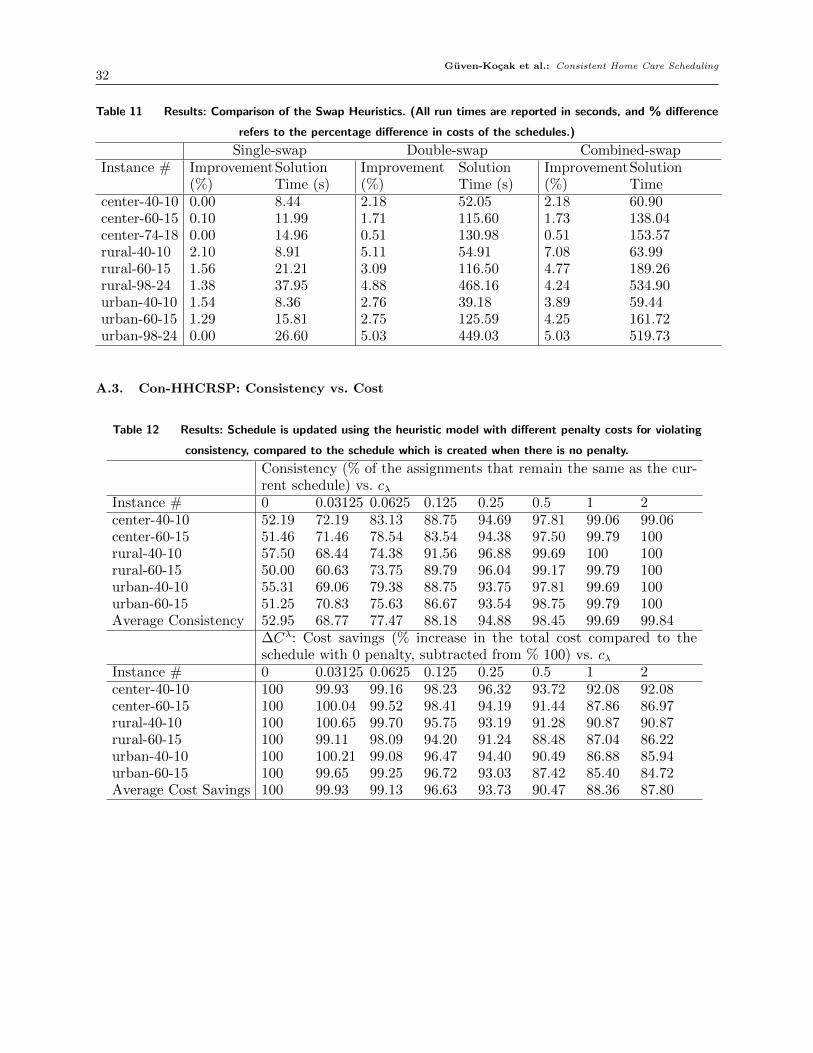
Guven-Kocak et al.: Consistent Home Care Scheduling32
Table 11 Results: Comparison of the Swap Heuristics. (All run times are reported in seconds, and % difference
refers to the percentage difference in costs of the schedules.)
Single-swap Double-swap Combined-swapInstance # Improvement
(%)SolutionTime (s)
Improvement(%)
SolutionTime (s)
Improvement(%)
SolutionTime
center-40-10 0.00 8.44 2.18 52.05 2.18 60.90center-60-15 0.10 11.99 1.71 115.60 1.73 138.04center-74-18 0.00 14.96 0.51 130.98 0.51 153.57rural-40-10 2.10 8.91 5.11 54.91 7.08 63.99rural-60-15 1.56 21.21 3.09 116.50 4.77 189.26rural-98-24 1.38 37.95 4.88 468.16 4.24 534.90urban-40-10 1.54 8.36 2.76 39.18 3.89 59.44urban-60-15 1.29 15.81 2.75 125.59 4.25 161.72urban-98-24 0.00 26.60 5.03 449.03 5.03 519.73
A.3. Con-HHCRSP: Consistency vs. Cost
Table 12 Results: Schedule is updated using the heuristic model with different penalty costs for violating
consistency, compared to the schedule which is created when there is no penalty.
Consistency (% of the assignments that remain the same as the cur-rent schedule) vs. cλ
Instance # 0 0.03125 0.0625 0.125 0.25 0.5 1 2center-40-10 52.19 72.19 83.13 88.75 94.69 97.81 99.06 99.06center-60-15 51.46 71.46 78.54 83.54 94.38 97.50 99.79 100rural-40-10 57.50 68.44 74.38 91.56 96.88 99.69 100 100rural-60-15 50.00 60.63 73.75 89.79 96.04 99.17 99.79 100urban-40-10 55.31 69.06 79.38 88.75 93.75 97.81 99.69 100urban-60-15 51.25 70.83 75.63 86.67 93.54 98.75 99.79 100Average Consistency 52.95 68.77 77.47 88.18 94.88 98.45 99.69 99.84
∆Cλ: Cost savings (% increase in the total cost compared to theschedule with 0 penalty, subtracted from % 100) vs. cλ
Instance # 0 0.03125 0.0625 0.125 0.25 0.5 1 2center-40-10 100 99.93 99.16 98.23 96.32 93.72 92.08 92.08center-60-15 100 100.04 99.52 98.41 94.19 91.44 87.86 86.97rural-40-10 100 100.65 99.70 95.75 93.19 91.28 90.87 90.87rural-60-15 100 99.11 98.09 94.20 91.24 88.48 87.04 86.22urban-40-10 100 100.21 99.08 96.47 94.40 90.49 86.88 85.94urban-60-15 100 99.65 99.25 96.72 93.03 87.42 85.40 84.72Average Cost Savings 100 99.93 99.13 96.63 93.73 90.47 88.36 87.80

Guven-Kocak et al.: Consistent Home Care Scheduling33
References
Beasley J, Krishnamoorthy M, Sharaiha Y, Abramson D, 2004 Displacement problem and dynamically
scheduling aircraft landings. Journal of the operational research society 55(1):54–64.
Bennett AR, Erera AL, 2011 Dynamic periodic fixed appointment scheduling for home health. IIE Transac-
tions on Healthcare Systems Engineering 1(1):6–19.
Cappanera P, Scutella MG, 2014 Joint assignment, scheduling, and routing models to home care optimization:
a pattern-based approach. Transportation Science 49(4):830–852.
Castillo-Salazar JA, Landa-Silva D, Qu R, 2014 Workforce scheduling and routing problems: literature survey
and computational study. Annals of Operations Research 1–29.
Coelho LC, Cordeau JF, Laporte G, 2012 Consistency in multi-vehicle inventory-routing. Transportation
Research Part C: Emerging Technologies 24:270–287.
Fikar C, Hirsch P, 2017 Home health care routing and scheduling: A review. Computers & Operations Research
77:86–95.
Foster BA, Ryan DM, 1976 An integer programming approach to the vehicle scheduling problem. Journal of
the Operational Research Society 27(2):367–384.
Groer C, Golden B, Wasil E, 2009 The consistent vehicle routing problem. Manufacturing & service operations
management 11(4):630–643.
Gutierrez EV, Vidal C, 2013 Home health care logistics management: Framework and research perspectives.
International Journal of Industrial Engineering and Management 4(3):173–182.
Haggerty JL, Reid RJ, Freeman GK, Starfield BH, Adair CE, McKendry R, 2003 Continuity of care: a
multidisciplinary review. BMJ: British Medical Journal 327(7425):1219.
Jensen TS, 2012 Application of metaheuristics to real-life scheduling problems. Philosophiae Doctor thesis,
Department of Mathematics and Computer Science, University of Southern Denmark, Odense, Den-
mark .
Jones E, Oliphant T, Peterson P, et al., 2001– SciPy: Open source scientific tools for Python, package: Hier-
archical clustering (scipy.cluster.hierarchy). URL http://www.scipy.org/, [Online; accessed 2017-05-
02].
Kovacs AA, Golden BL, Hartl RF, Parragh SN, 2014 The generalized consistent vehicle routing problem.
Transportation Science 49(4):796–816.
Macdonald T, Dorner K, Gandibleux X, 2009 Metaheuristics for the consistent nurse scheduling and routing
problem .
NHPCO, 2016 Nhpcos facts and figures - hospice care in america. Technical report, National Hospice and
Palliative Care Organization.
Nickel S, Schroder M, Steeg J, 2012 Mid-term and short-term planning support for home health care services.
European Journal of Operational Research 219(3):574–587.

Guven-Kocak et al.: Consistent Home Care Scheduling34
Potvin JY, Rousseau JM, 1993 A parallel route building algorithm for the vehicle routing and scheduling
problem with time windows. European Journal of Operational Research 66(3):331–340.
Wong RT, 2008 Vehicle routing for small package delivery and pickup services. The Vehicle Routing Problem:
Latest Advances and New Challenges, 475–485 (Springer).