holdup with subsidized investment - fm · holdup with subsidized investment ... crawford, and...
TRANSCRIPT

Holdup with Subsidized Investment
Makoto Hanazono∗
Institute of Economic Research, Kyoto University†
March 30, 2004
Abstract
A holdup model is analyzed in which one party, the seller, has an investment projectthat the other party, the buyer, can subsidize. The investment project remains theseller’s; she cannot transfer her entire control rights to it. In particular, she can alwaysrefuse to allow the buyer to subsidize her investment if the subsidy would put the buyerin too strong a bargaining position ex post. Even with the subsidization opportunity,the holdup inefficiency is still present, except in the special cases in which one partyhas all the bargaining power. The adoption of a contract, however, allows full efficiencyto be achieved more generally. In particular, if the seller’s investment project imposesa positive externality on the buyer but does not reduce her own production costs, abuyer’s option contract exists that achieves full efficiency. This is in contrast to theresult of Che and Hausch (1999) that without a subsidization opportunity, contractinghas no value in this “purely cooperative” case. If the investment lowers the seller’s costsas well as raises the buyer’s value, whether full efficiency can be achieved depends onhow cooperative the investment is. Full efficiency can be achieved if the cooperativenessof the investment is either sufficiently high or sufficiently low.
1 Introduction
Coase’s (1937) celebrated work addresses the key insight that transaction costs play a central
role in the theory of the firm and directs researchers to look at sources of transaction costs.
As pointed out by Klein, Crawford, and Alchian (1978) and Williamson (1985), one of the
most important transaction costs is associated with the so-called holdup problem.
The holdup problem occurs if the value of a transaction between two parties depends
on an ex ante investment. It arises under two conditions. First, the investment must be∗This article is developed from a chapter of my Ph.D. dissertation submitted to the University of Penn-
sylvania. I am grateful to Hideshi Itoh, George Mailath, Sönje Reiche, Rafael Rob, Ilya Segal, TadashiSekiguchi, Manuel Willington, Huanxing Yang and seminar participants at Penn, Pompeu Fabra, and Con-tract Theory Workshop at Kyoto for helpful comments, discussions and suggestions. I am truly indebted toSteve Matthews, my dissertation advisor, for his invaluable advice, support and guidance.
†Address: Sakyo-ku, Kyoto, 606-8501 Japan. Email: [email protected].
1
relationship specific, i.e., the benefit of investment must be substantially reduced if the par-
ties change trading partners. Because of this opportunity cost of changing trading partners,
the parties are locked into the relationship once the investment is made. Second, the con-
tract must be incomplete, i.e., it must be impossible to specify every relevant contingency
in the contract.1 This leads to ex post bargaining in which the non-investing party can
successfully demand a part of the investment benefit, i.e., the non-investing party “holds
up” the investing party. Anticipating this ex post opportunistic behavior, the investing
party underinvests.2
To the best of the author’s knowledge, the existing literature on the holdup problem
adopts the following common assumption: the control right to each investment project be-
longs exclusively to one party. That is, the investment level in a project is assumed to be
determined solely by the party who owns the control right to that project. If a different
party is supposed to choose the investment level, the control right has to be transferred,
say, through integration.
In reality, however, there are investment projects whose control rights are not so exclu-
sive. Some investment projects entail a subsidization opportunity by a party who is allowed
to invest by the controlling, “owning” party. In Asanuma (1989) such evidence regarding
components design can be found in the Japanese automaker-supplier relationships; some
automakers, which once bought some simple parts from their suppliers, later purchased
parts in “increasingly more assembled forms” (Asanuma (1989, p14)). This fact shows that
such investment project as designing is not exclusive, and can be subsidized.3 Bart (1989)
documents that component designing for Xerox products has been shifting from Xerox to its
suppliers. Holmström and Roberts (1998) describe the case of human capital investment;
“The automakers also assist the suppliers in improving productivity and lowering costs;
technical support engineers are a major part of the automakers’ purchasing staff, and they
spend significant amounts of time at the suppliers’ facilities.”4
1This is based on the empirical observation that, in many cases, there are no written ex ante contractson details of trade between, say, an automotive assembler and parts suppliers. This has led researchers tosimply assuming there is no ex ante contract.
2Various ways to remedy this inefficiency problem have been proposed. For the related work, see theliterature review in section 2.
3He classifies suppliers producing customized parts into two category; one with “drawings supplied” bythe automaker, and the other with “drawings approved.”
4We can also find discussions and cases for subsidization in other literature. Hart (1995, pp.69-70n)points out that physical investment projects are often “alienable”: if its owner permits, another party caninvest in the project. Coase (2000) provides evidence of subsidization by General Motors (p. 28); “It isevident that what Sloan was referring to was not a dispute over whether the Fisher Body plants should belocated near the General Motors assembly plants but one over which organization should put up the capitalrequired to do it. ... The cost was borne by General Motors. No doubt this also happened for many of the
2

A subsidization opportunity generates new issues regarding the parties’ investment be-
havior. The first issue is to investigate the non-owning party’s incentives to invest. Once
this party is allowed to invest, the party may wish to contribute toward a more efficient
investment level than the owning party wishes to achieve. This new incentives to invest
by the non-owning party might be undermined by the owning party’s holdup opportunity,
which arises if subsidization occurs. The second issue is to investigate whether the owning
party actually allows the other party to subsidize. The owning party might find that refus-
ing to allow subsidization is optimal. It is thus not clear whether inefficiency property due
to holdup is remedied if subsidization is possible.
This paper incorporates subsidization into a standard holdup model. Specifically, we
analyze a holdup model in which one party, the seller, has an investment project that
the other party, the buyer, can subsidize.5 The investment project remains the seller’s;
she cannot transfer her entire control rights to it. The buyer can subsidize the project by
directly making the investment if the seller permits him. We keep the following three typical
assumptions in the standard holdup literature. (i) No aspect of investment is contractible;
a contract cannot specify how much is invested or who makes the investment. (ii) Trade
quantities and payments are contractible. This allows the parties to sign a menu contract
from which a pair of quantity and payment is chosen according to the choice rule specified
in the contract (such as buyer-option, seller-option, or more complicated rules).6 (iii) The
parties cannot commit not to renegotiate the contract; when they find the chosen trade
quantity to be ex post inefficient, the parties revise it to the efficient quantity. This leads
to bargaining over the additional surplus generated by renegotiation, with the status quo
payoff determined by the original contract.
We restrict attention to the case where the subsidizing party has the same investing
technology as the owning party. As a consequence, the gains from investment only depend
on the total level of investment but not on how much each party contributes to the to-
tal investment. This is clearly a strong restriction, but not entirely unrealistic. In fact,
Asanuma (1989) documents that, for such parts as seats, Japanese automakers possess de-
tailed information about processes of producing them. This suggests that both parties have
approximately the same cost structure in designing these parts.
The main result of this paper is that a buyer-option contract exists that achieves full
other Fisher Body plants.”5By symmetry, we can treat the case where the buyer owns the project and the seller may subsidize,
which corresponds to the above case in Asanuma (1989).6Both parties are assumed to send verifiable messages to the court without costs. A pair of trade and
payment can be contingent on those messages in general. An option contract requires a message (or request)from one party; for example, a buyer-option contract allows the buyer to choose a pair among the alternatives.
3
efficiency if the seller’s investment project imposes a positive externality on the buyer but
does not reduce her own production costs, i.e., the investment is “purely cooperative.”
Moreover, full efficiency can be achieved even if the cooperativeness of the investment is
not pure, but just sufficiently high. This is in contrast to the result of Che and Hausch
(1999) that without a subsidization opportunity, contracting has no value in these highly
cooperative cases.
The effect of introducing a subsidization opportunity is twofold. First, it reduces the
holdup inefficiency in general. The induced investment level when subsidization is possible
is (weakly) more efficient than when subsidization is not possible. This is because the seller
can make an additional investment even after the buyer invests and hence a positive level
of subsidization occurs if and only if both parties are better off with it.7 This implies that
if full efficiency is achieved when subsidization is not possible, it is still achievable after
introducing a subsidization opportunity. In particular, the following result of Edlin and
Reichelstein (1996) holds even when subsidization is possible: if the seller’s investment only
reduces her own production cost but not improve the buyer’s valuation, i.e., the investment
is “purely selfish”, a noncontingent contract exists such that the seller invests at the first-
best level.
Second, a subsidization opportunity can cause the seller to behave opportunistically.
She can always refuse to allow the buyer to subsidize her investment if the subsidy would
put the buyer in too strong a bargaining position ex post. This shows that a subsidization
opportunity does not simply flip the role of parties, i.e., it cannot transfer the seller’s project
to the buyer.
Subsidization creates two new effects of contracting. First, a contract affects the buyer’s
incentive to subsidize (the incentive effect on the buyer’s subsidization). If a contract can
change the status quo point of ex post bargaining in favor of the buyer, it will improve the
incentive. This is a mirror image of the effect of a contract on the seller’s incentive to invest.
Second, a contract affects the seller’s incentive to permit subsidization (the incentive effect
on the seller’s permission). This is due to the new seller opportunism discussed above. An
optimal contract must take these two effects into account.
Without the seller opportunism, full efficiency for a purely cooperative investment would
be rather trivial. It would be achieved as a corollary of the result of Edlin and Reichel-
stein (1996); the seller’s purely cooperative investment would be just the buyer’s purely
selfish investment when subsidization is possible, and thus a noncontingent contract would
7The buyer subsidizes if and only if the benefit of subsidizing exceeds that of foregoing the opportunityand letting the seller invest. The seller allows the buyer to invest if and only if the resulting subsidizedinvestment gives her more profit than when she does not allow subsidization.
4
induce the buyer to invest efficiently. However, Edlin-Reichelstein’s noncontingent contract
indeed induces the seller to refuse subsidization, and results in an inefficient investment.
To achieve full efficiency in this purely cooperative case, a contract needs to give the right
incentive to the buyer to subsidize efficiently, and the right incentive to the seller to allow
the buyer to invest. It is shown in the analysis that a buyer-option contract does this but
no noncontingent contract does.
The important implication of these results is that the transaction cost associated with
holdup disappears if the seller’s investment is highly cooperative and can be subsidized by
the buyer. It is also shown that the holdup problem is solved by adopting a contract if
the seller’s investment has a small externality (i.e., highly selfish cases). Holdup therefore
causes no inefficiency if the investment imposes either a very small or a very large positive
externality. This paper provides a new evaluation of the transaction cost due to holdup
when a subsidization opportunity is available.
The structure of this paper is the following. The related literature is reviewed in section
2. The set up of the model is presented in section 3. In section 4, we discuss the holdup
problem and underinvestment issues with subsidization. Section 5 provides contractual
remedies to the holdup inefficiency in the purely selfish and the purely cooperative cases.
Section 6 deals with hybrid cases by giving a specific example. In section 7, a generalization
of the results in section 6 follows. Concluding remarks are addressed in section 8.
2 Related Literature
Holdup The literature on solutions to the holdup problem can be classified into two
groups according to the degree of incompleteness of contracts.8 The first group assumes that
no aspect of a transaction is ex ante contractible. The only ex ante contractible variables
are property/control rights and hence solutions to holdup take such forms as integration
(Klein et al.(1978), Williamson (1985)) and allocation of property rights (Grossman and
Hart (1986), Hart and Moore (1990)).
This paper belongs to the second group that assumes some aspects of a transaction,
such as the quantity to be traded, are contractible. Some authors solve the holdup problem
by giving full bargaining power to one party through contracting. For example, Chung
8The definition of incompleteness of contracts varies among researchers. We simply define a contract tobe incomplete if variables are noncontractible. Alternatively, a contract “becomes” incomplete if the partiesoptimally leave contingencies open. That is, specifying more contingencies is valueless in disciplining theparties’ behavior, due to the complexity of the state of the world (Segal (1999) and Hart and Moore (1999))or strategic ambiguity (Bernheim and Whinston (1998)), for example. See also Tirole (1999) for discussion.
5
(1991) and Aghion, Dewatripont and Rey (1994) assume the ex post bargaining procedure
is contractible.9
This paper’s approach is closest to that of Edlin and Reichelstein (1996) and Che and
Hausch (1999). These papers assume that the ex post bargaining procedure is not con-
tractible; bargaining is governed by an exogenous bargaining procedure.10 In this case,
whether full efficiency can be achieved depends on how cooperative the investment is. Edlin
and Reichelstein (1996) show that full efficiency can be achieved if the investment is purely
selfish. Che and Hausch (1999), on the other hand, prove that contracting has no value to
improve efficiency if the investment is highly cooperative.
None of these papers considers investments that can be subsidized.
Delegation Subsidization in our model is a delegated action: the party that has the
authority to control the investment is able to allow the other party to invest. Delegation of
authority is extensively analyzed by Aghion and Tirole (1997). More related to this paper
is the one by Aghion, Dewatripont, and Rey (2002). They consider a non-contractible
but transferable control; the control of an action can be delegated even when a contract
cannot specify this delegation. They analyze a repeated interaction of a principal and
an agent in which the agent has private information. They find that in equilibrium, the
principal delegates her action to the agent in an earlier period, in order for the agent to
build a reputation. Our model makes a similar assumption on control rights, but differs by
examining how a contract affects the incentive to subsidize.
Partnership The structure of our model is similar to that of partnership (Holmström
(1982), Legros and Matthews (1993)) in which several parties contribute to the same project
and share the benefits from it. In those models, the agents’ efforts affect a verifiable signal
upon which a contract can be written to induce efforts. In our model, there is no such
verifiable signal of the exerted effort/investment levels. The contractible variables instead
affect the parties’ ex post bargaining position which may indirectly induce the desired effort
levels. The partnership models also assume that each agent can freely contribute to the
common project, whereas our model assumes the investment project is owned by an agent
who is able to prohibit others from investing in it.
9These papers solve the holdup problem in a two-sided investment environment. Since giving full bar-gaining power renders the right incentive to invest to one party, an additional instrument (e.g., a specificperformance contract) is required to provide an incentive to the other.10These papers take the bargaining procedure as a black box, and typically assume that the outcome of
bargaining is a generalized Nash bargaining solution.
6

Mechanism Design with Renegotiation This paper applies results from the literature
on mechanism design with renegotiation. The fundamental theoretical contribution is made
by Maskin and Moore (1999), who give characterization theorems for implementability in
a general setting. Segal and Whinston (2002) derive a convenient representation theorem
for risk-neutral, quasilinear utilities and apply it to the standard holdup problem. We use
some of their results.
3 Model
Primitives. A seller produces an intermediate good for a buyer. In advance of trade, the
seller can make a relationship-specific investment. We assume that the buyer can subsidize
this investment. The investment may affect the quality of the good or the costs of producing
it. Further details of the investment are discussed below. Let (q, t) denote the quantity
of the intermediate good to be traded and the monetary transfer from the buyer to the
seller, respectively. The investment level x is measured in terms of money. Let v (q, x) and
c (q, x) denote the buyer’s ex post valuation function and the seller’s ex post cost function
respectively.11 Let us assume v and c are C2-functions defined on [0, qmax]× [0, xmax] withv(0, x) = c(0, x) = 0.The buyer’s valuation v is strictly increasing and strictly concave in q,
and increasing and concave in x. The seller’s cost c is strictly increasing and strictly convex
in q, and decreasing and convex in x. The parties’ payoffs are quasi-linear in the transfer t
and investment cost.
The ex post surplus generated by (q, x) is S(q, x) = v(q, x)− c(q, x). This surplus S(q, x)
is by assumption strictly concave in q, and thus for each x, a unique maximizer q∗(x) ofS(q, x) exists. We call it the ex post efficient trade given investment level x. To characterize
it by a first-order condition, we assume 0 < q∗(x) < qmax. It is continuously differentiable
by the implicit function theorem. Let S∗ (x) = S (q∗(x), x) denote the ex post efficientsurplus given investment level x. The envelope theorem implies S∗ is increasing, i.e.,
S∗0(x) = vx(q∗(x), x)− cx(q
∗(x), x) ≥ 0.
The first-best or efficient investment level is a solution to
maxx
S∗(x)− x.
11These v and c are the value functions derived by the buyer’s and the seller’s optimization problems.The valuation function v, for example, measures the buyer’s maximized profits of his final products, givenhis technological constraint and q units of intermediate good. The level of investment x may also affect thequality of an intermediate good, and thus the buyer’s profits.
7
We assume that S∗(x) is strictly concave in order to have a unique solution to the prob-lem.12 Let x∗ denote the efficient investment and assume x∗ > 0 (otherwise there is no
underinvestment problem).
In addition to these assumptions, let us suppose the following complementarity condi-
tions hold: (i) vqx > 0 for all (q, x)unless vx ≡ 0, and (ii) cqx < 0 for all (q, x)unless cx ≡ 0.Thus, as the investment level increases, the buyer’s marginal valuation of trade increases
and the seller’s marginal cost of production decreases, provided the investment affects the
valuation or cost. For example, we must have vqx ≡ 0 if the investment has no effect on thebuyer’s valuation, i.e., vx ≡ 0.
Investment The key assumption is that the seller can allow the buyer to invest. The seller
may lend the buyer the key to her facility, or let her workers provide necessary expertise to
the buyer. The buyer can then invest in the seller’s project. It is natural to assume that
the seller can invest more after the buyer invests;13 the seller can postpone producing the
good if she observes the buyer’s investment is inadequate, and wants to make an additional
investment.
We assume that the buyer has the same investment technology as does the seller, so
that the benefit of investment does not depend on who invests. For a concrete example,
consider a situation in which the seller can buy and customize a machine to be used in
her facility. The buyer may well buy and customize the same machine at the same cost if
the seller provides necessary expertise. As another example, consider that the seller can
invest in her worker’s skill for inspection of her customized products. The buyer can send
his worker in the seller’s place to acquire the skill at his own cost if the seller permits him
to do so. This assumption implies that the total investment level is the sum of the buyer’s
and the seller’s investments.
Subsidization is a delegated action in our model. It is not a side payment from the buyer
to the seller. Note that a contract cannot force the seller to invest because the investment
is unverifiable (discussed below). If the buyer just gives money to the seller, the seller
will “take the money and run.” The buyer needs to spend money by directly making the
investment.12Strict concavity of S∗ is implied if, for example,
|vxx − cxx| > (vqx − cqx)2
vqq − cqq,
for all (q, x). Thus if v − c is sufficiently concave, S∗ is strictly concave.13The results of this paper will not change if the seller can reduce the investment level.
8

Accordingly, we consider the following extensive game at the investment stage:
1. The seller decides whether or not the buyer is allowed to invest.
2. If allowed, the buyer decides how much to invest, xb ≥ 0. If not allowed to invest,xb = 0.
3. After observing xb, the seller decides how much to invest, xs ≥ 0. The total investmentlevel is then x = xb + xs.
The buyer’s and seller’s investment costs are xb and xs, respectively, since the investment
is measured by money. The investment costs are sunk once they are made.
In the subsequent analysis, we will see that the nature of the seller’s investment affects
the possibility of contractual remedy to the holdup problem. Following Che and Hausch
(1999), the investment is called selfish if it reduces the seller’s cost of production, i.e.,
cx < 0 for q > 0. Alternatively, the investment is called cooperative if it enhances the
buyer’s valuation, i.e., vx > 0 for q > 0. Note that it can be both selfish and cooperative
at the same time. Given the maintained assumptions, there are three cases to consider: the
purely selfish case, vx = 0 and cx < 0; the purely cooperative case, vx > 0 and cx = 0; and
the hybrid case, vx > 0 and cx < 0.
Timing The time line of our model is as follows.
Parties signa contract
InvestmentsContract termsare chosen
Renegotiation Trade
↓ ↓ ↓ ↓ ↓––––––––––––––––––––––––––––—→
` −−−Ex ante−−−− a ` −−−− Interim−−−− a Ex post
Contracts Following the holdup literature, we assume that both parties observe the in-
vestment, but it is unverifiable to any third party. It is often too costly to verify relationship-
specific skills, expertise, or even physical investments. The buyer’s valuation and the seller’s
cost of production are also assumed to be unverifiable. If they are verifiable, the third party
can infer the investment from those variables. The quality of the intermediate good is not
verifiable either, if the investment enhances it.
A transaction is assumed to be verifiable, and a contract can thus specify a quantity to be
traded and a monetary transfer. Following the implementation literature (e.g., Maskin and
9
Moore (1999)), we allow each party to send arbitrary messages to choose the contract terms.
A contract is then generally a message game©q¡mb,ms
¢, t¡mb,ms
¢ªwhere mi ∈ M i,
i = b, s, is party i’s message.14 One typical message game is the “shoot-the-liar” mechanism,
in which the parties have to pay a huge penalty when the messages disagree. This mechanism
works well when the parties can commit not to renegotiate, but it does not work when they
cannot commit (see Che and Hausch (1999) and Maskin and Tirole (1999)).
The following are relevant particular contracts. A noncontingent contract : q(mb,ms) =
q, t(mb,ms) = t, ∀mb,∀ms. The null contract : q(mb,ms) = 0, t(mb,ms) = 0, ∀mb,∀ms.
The null contract is equivalent to not adopting a contract. A buyer-option contract :
q(mb,ms) = qb(mb), t(mb,ms) = tb(mb), ∀mb,∀ms. A seller-option contract is defined
similarly.
Renegotiation We suppose that the parties are unable to commit not to renegotiate a
contract. If the chosen contract terms (q0, t0) = (q¡mb,ms
¢, t¡mb,ms
¢) are not ex post
efficient, i.e., q0 6= q∗(x), they renegotiate. The new transfer level is determined so that
the renegotiation surplus S∗(x)− S (q, x) is split according to exogenous bargaining shares
(λb, λs), where λb, λs ≥ 0 and λb + λs = 1.15 This renegotiation defines the buyer’s and the
seller’s interim payoffs for the pre-renegotiated outcome (q0, t0) and the investment level x
as follows:
v(q0, x)− t0 + λb[S∗ (x)− S(q0, x)] ≡ rb(q0, x)− t0, (1)
t0 − c(q0, x) + λs[S∗ (x)− S(q0, x)] ≡ rs(q0, x) + t0. (2)
The functions rband rs defined above are used in the subsequent analysis.
Ex post efficient renegotiation implies that
rb(q0, x) + rs(q0, x) ≡ S∗(x) for any q0.
That is, given the total investment level, the sum of the interim payoffs is the same regardless
of the outcome of the message game. This shows that a contract specifies a two-person zero-
sum game for any given investment level. By the minimax theorem, each player’s payoff in
any Nash equilibrium is the minimax value.16
14We assume that the messages are sent simultaneously. Extensive games may help achieve uniqueness ofequilibrium of the message game, but do not help improve efficiency (see footnote 16).15This assumption on bargaining is as in Che and Hausch (1999) and Segal and Whinston (2002). Edlin
and Reichelstein (1996) take (λb, λs) to be functions of investment and uncertainty realization. Maskin andMoore (1999) assume an arbitrary sharing rule that is efficient and individually rational. Hart and Moore(1988), MacLeod and Malcomson (1993) and Nöldeke and Schmidt (1995) specify the bargaining procedurein a non-cooperative manner.16This gives a justification for the claim in footnote 14 that the use of extensive-form message game
10

Ex ante Payoffs and Equilibrium Investments Suppose the parties adopt a con-
tract©q¡mb,ms
¢, t¡mb,ms
¢ª. Each party chooses its message given an investment pair,
(xb, xs). Let (mb∗(xb, xs),ms∗(xb, xs)) denote an equilibrium of the message game given the
investment.17 Define Rb(xb, xs) and Rs(xb, xs) by
Rb(xb, xs) = rb(q(mb∗(xb, xs),ms∗(xb, xs)), xb + xs)− t(mb∗(xb, xs),ms∗(xb, xs)),
Rs(xb, xs) = rs(q(mb∗(xb, xs),ms∗(xb, xs)), xb + xs) + t(mb∗(xb, xs),ms∗(xb, xs)).
These are the parties’ revenues for each investment pair (xb, xs), given an equilibrium of
the message game. We call them the buyer’s and the seller’s ex ante revenues respectively.
The choice of equilibrium does not affect the revenues because all equilibria give the same
minimax payoffs to the parties.
At the investment stage, the buyer and the seller invest xb and xs respectively. Recall
that xband xs are measured in terms of money. Therefore the buyer’s and the seller’s ex
ante payoffs at the investment stage are, respectively,
Rb(xb, xs)− xb,
Rs(xb, xs)− xs.
The equilibrium investments are given by a subgame perfect equilibrium in the invest-
ment stage.
4 Holdup Problem
In this section, we show that allowing subsidization does not entirely eliminate the un-
derinvestment problem due to holdup except for a special case in which the buyer has
full bargaining power. We also show that the equilibrium investment level becomes more
efficient by allowing subsidization, given any contract.
If the contract is null, the parties have no obligation to trade. Nevertheless, for any
investment level x, trade will be beneficial ex post. The parties then trade and share the ex
post efficient surplus. The ex ante payoffs are
Rb(xb, xs)− xb = λbS∗(xb + xs)− xb,
Rs(xb, xs)− xs = λsS∗(xb + xs)− xs.
does not help improve efficiency: the normal form representation of the extensive form game has a Nashequilibrium that corresponds to a subgame perfect equilibrium of the extensive form game. The equilibriumpayoff is the minimax of the normal form game.17The equilibrium strategies might be mixed strategies and in such cases, we need to modify the notation.
The payoffs are also the expected value with respect to the mixed strategies. The following analysis remainsvalid if the parties are risk-neutral. For notational simplicity, we keep the notation as in the text.
11
What does an equilibrium look like? Suppose first that the seller’s bargaining share
λs is large. In equilibrium the seller invests and the buyer does not. Even if the buyer
is allowed to invest, he finds it beneficial to forgo this opportunity since the seller will
make substantial (if not necessarily efficient) investment. The buyer subsidizes the seller’s
project only if his payoff from investing exceeds his payoff from forgoing the opportunity.
Alternatively, suppose that the buyer has full bargaining power (λb = 1). He invests at the
first-best level if he is permitted. The seller permits him to invest in equilibrium since she
is indifferent between doing and not doing so.
In general, the buyer’s payoff from investing is increasing in his bargaining share λb
whereas his payoff from forgoing is decreasing (since the seller’s investment is decreasing).
The seller’s willingness to permit subsidization grows in λb since the buyer’s investment is
increasing in λb. This implies that there is a threshold of λb over which the buyer will invest
at some positive level in equilibrium.
The underinvestment problem remains unless either party has full bargaining power.
To see this, consider first the case in which the seller makes a positive investment. Notice
that she always invests at the margin. The investment level is efficient in this case only if
she has full bargaining power. Alternatively, consider that the seller does not invest; the
investment is entirely subsidized by the buyer. It is clear that the investment is efficient only
if he has full bargaining power. This shows that the underinvestment problem disappears
by allowing subsidization only when λb = 1.
Inefficiency due to holdup is (weakly) reduced by allowing subsidization. Suppose first
that the buyer does not invest in equilibrium. It is straightforward that the investment level
must be the same as the one when subsidization is not possible. Alternatively, suppose that
the buyer invests in equilibrium. This must imply the buyer’s equilibrium payoff must be
more than his payoff from forgoing, and the seller’s equilibrium payoff must also be more
than her payoff from refusing to permit subsidization. In either of the off-path outcomes
reached by forgoing or refusing, the seller would invest at the same level as she would when
subsidization is not possible. This implies that allowing subsidization must be Pareto-
improving and therefore the equilibrium investment must be more efficient. This argument
does not rely on not adopting a contract. It holds even when a contract is adopted.
We summarize these results as follows:
Proposition 1 If a contract is not adopted, the parties underinvest except in the caseswhere λs = 1 or λb = 1.
12
Proposition 2 Given any contract, an equilibrium investment becomes (weakly) more ef-
ficient by allowing subsidization.
Remark 1 In the preceding analysis the characteristics of investment do not matter. Incontrast, the following analysis shows that the effectiveness of contracting depends on the
degree to which the investment is cooperative or selfish.
Proposition 1 leads to our analysis of contractual remedies to the underinvestment prob-
lem.
5 Two Polar Cases
Contracting affects the buyer’s and the seller’s ex ante revenue functions and therefore alters
their incentives to invest. This is because a contract determines the status quo point of the
bargaining at the renegotiation stage, which is affected by the parties’ investment decision.
The effect of investment on the status quo depends on three things: the primitive
functions v and c, the bargaining shares (λb, λs), and the contract the parties sign. In this
section we investigate the purely selfish and the purely cooperative cases separately. The
hybrid cases are analyzed in the following sections.
Purely Selfish Case Edlin and Reichelstein (1996) show that in the purely selfish case
with no subsidization opportunity, a noncontingent contract achieves full efficiency. Under
no uncertainty, the noncontingent contract sets the trade equal to the ex post efficient trade
for the first-best investment level, q∗(x∗). The transfer is irrelevant for incentives.Proposition 2 implies that the same contract also achieves efficiency when subsidization
is possible. Thus the following proposition obtains:
Proposition 3 In the purely selfish case, a noncontingent contract that specifies the ex postefficient trade for the first-best investment level induces the seller to invest efficiently.
Purely Cooperative Case In this subsection the seller’s cost function depends only on
q, and we write it simply as c(q).
Che and Hausch (1999) show that if the investment is purely cooperative, contracting
cannot improve the investing party’s incentives to invest. Therefore, without a subsidiza-
tion opportunity, the null contract is optimal. This implies that unless the seller has full
bargaining power, full efficiency cannot be achieved.
13

By allowing subsidization, one might conjecture that the seller’s purely cooperative
investment becomes the buyer’s purely selfish investment, and that a noncontingent contract
analogous to Proposition 3 thus achieves full efficiency. The following proposition shows
that this conjecture is not true.
Proposition 4 In the purely cooperative case, full efficiency cannot be achieved by a non-contingent contract unless either party has full bargaining power.
Proof. See Appendix. ¥
To see that the above conjecture is not true, consider that a noncontingent contract
(q = q∗(x∗), t) is adopted as in Edlin and Reichelstein (1996). If subsidization transformsseller’s purely cooperative investment to a purely selfish investment for the buyer, this
contract can induce the buyer to entirely make the first-best investment. The seller must
therefore allow the buyer to invest. If the buyer invests at the first-best level, the ex post
efficient trade is q∗(x∗) as in the contract. There is no renegotiation in this case. Supposealternatively the seller refuses to allow the buyer to invest and does not invest afterwards.
The resulting investment level is then zero. Under the noncontingent contract, renegotiation
must occur and the seller can hold up the buyer through renegotiation; she can successfully
demand part of the renegotiation surplus. By pure cooperativeness, i.e., c (q, x) = c (q), the
seller’s payoff from the status quo is the same for any investment. The seller will therefore
be better off if she does not allow the buyer to invest than if she does. This shows that the
contract cannot induce the buyer to invest efficiently in equilibrium. Proposition 4 shows
that, in the purely cooperative case, any other noncontingent contract would not work to
achieve the first-best, unless one party has full bargaining power.
The buyer needs the seller’s permission to subsidize. The seller’s right to give permission
provides extra opportunities for the seller to hold up the buyer. Thus in order to achieve
the efficient investment in the purely cooperative case, the parties need to write a contract
which avoids this extra holdup problem.
The next proposition shows, in this purely cooperative case, full efficiency is achievable
by adopting a buyer-option contract.
Proposition 5 In the purely cooperative case, the following buyer-option contract inducesthe buyer to invest entirely at the first-best level in a subgame perfect equilibrium: “The
buyer chooses a quantity q and pays c(q) to the seller,” or formally,
q(mb,ms) = mb and t(mb,ms) = c(mb).
14

Proof. Given this option contract, if x is the total investment, the buyer’s revenue fromchoosing q is,
v (q, x)− c (q) + λb[S∗ (x)− (v (q, x)− c (q))]
= (1− λb)(v (q, x)− c (q)) + λbS∗(x)
= λsS (q, x) + λbS∗ (x) .
The buyer therefore chooses q = q∗(x), the maximizer of S(q, x). The buyer’s ex ante revenueequals the ex post efficient surplus, and correspondingly the seller’s ex ante revenue is zero
for any investment level. Thus the buyer’s and the seller’s ex ante payoffs are, respectively,
Rb(xb, xs)− xb = S∗(xb + xs)− xb,
Rs(xb, xs)− xs = −xs.
The seller does not care about the buyer’s investment level, and so she will let the buyer
invest. The buyer invests at the first-best level since he anticipates that the seller will make
no investment afterwards. ¥
Given the buyer-option contract of Proposition 5, the buyer pays the exact cost of
whatever output he chooses. This implies that the seller’s payoff from the status quo is
always zero for any choice of the buyer and the seller’s ex ante revenue is thus just the share
of the renegotiation surplus. The buyer can always avoid renegotiation by choosing the
ex post efficient trade, which leads to no renegotiation and leaves no revenue to the seller.
The buyer’s ex ante revenue then coincides with the ex post efficient surplus so that the
buyer has an incentive to invest efficiently. On the seller’s side, the level of investment does
not affect her revenue, so she is indifferent between allowing and not allowing the buyer to
invest.
The same conclusion obtains even if we modify the contract so that the buyer needs to
pay c(q) plus a constant k for any choice of q. This contract achieves the same outcome as
would the outright purchasing of the investment project by the seller at price k, despite the
fact that the contract does not fully transfer the investment control right to the buyer.
Optimal Option Contracts of Finite Alternatives The contract in Proposition 5
has continuum of alternatives. This raises the following question; is it possible to construct
a simpler contract that induces the first-best investment? Here we study how to construct
a buyer-option contract of finite alternatives that achieves the first-best.
15
The contract in Proposition 5 induces the following two key equilibrium properties: (i)
the buyer will receive the entire surplus if the investment is efficient, and (ii) the seller is
indifferent between allowing and not allowing the buyer to invest. The first property obtains
since the buyer-option contract contains (q∗(x∗), c(q∗(x∗))); if the efficient investment ismade, the buyer chooses this alternative that is ex post efficient and that leaves no surplus
to the seller. The second property obtains since the contract contains (q∗(0), c(q∗(0))); theseller would make no investment if she were to refuse, and the buyer would then choose this
alternative.
One may then wonder whether a buyer-option contract with two options, (q∗(0), c(q∗(0)))and (q∗(x∗), c(q∗(x∗))), induces the same equilibrium outcome as the original buyer-option
contract. This depends on the seller’s off-path behavior; if she makes no investment after
refusing, the first-best outcome follows. However, she may have an incentive to invest after
refusing, as the following argument shows.
The seller’s incentives to invest is associated with her revenue function. For the two-
alternative buyer-option contract, she receives her share of the smaller one of two possible
renegotiation surpluses, namely,
Rs(xb, xs;λs) = min{λs(S∗(x)− S(q0, x)), λs(S∗(x)− S(q1, x))}
where x = xb + xs, q0 = q∗(0) and q1 = q∗(x∗).18 We thus identify Rs as a function on
the total level of investment, x, and the bargaining share, and write it as Rs(x;λs) by a
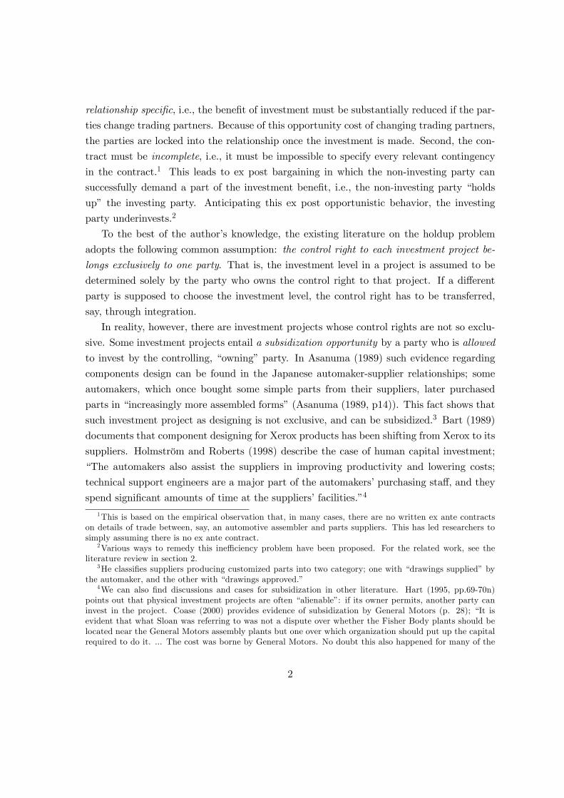
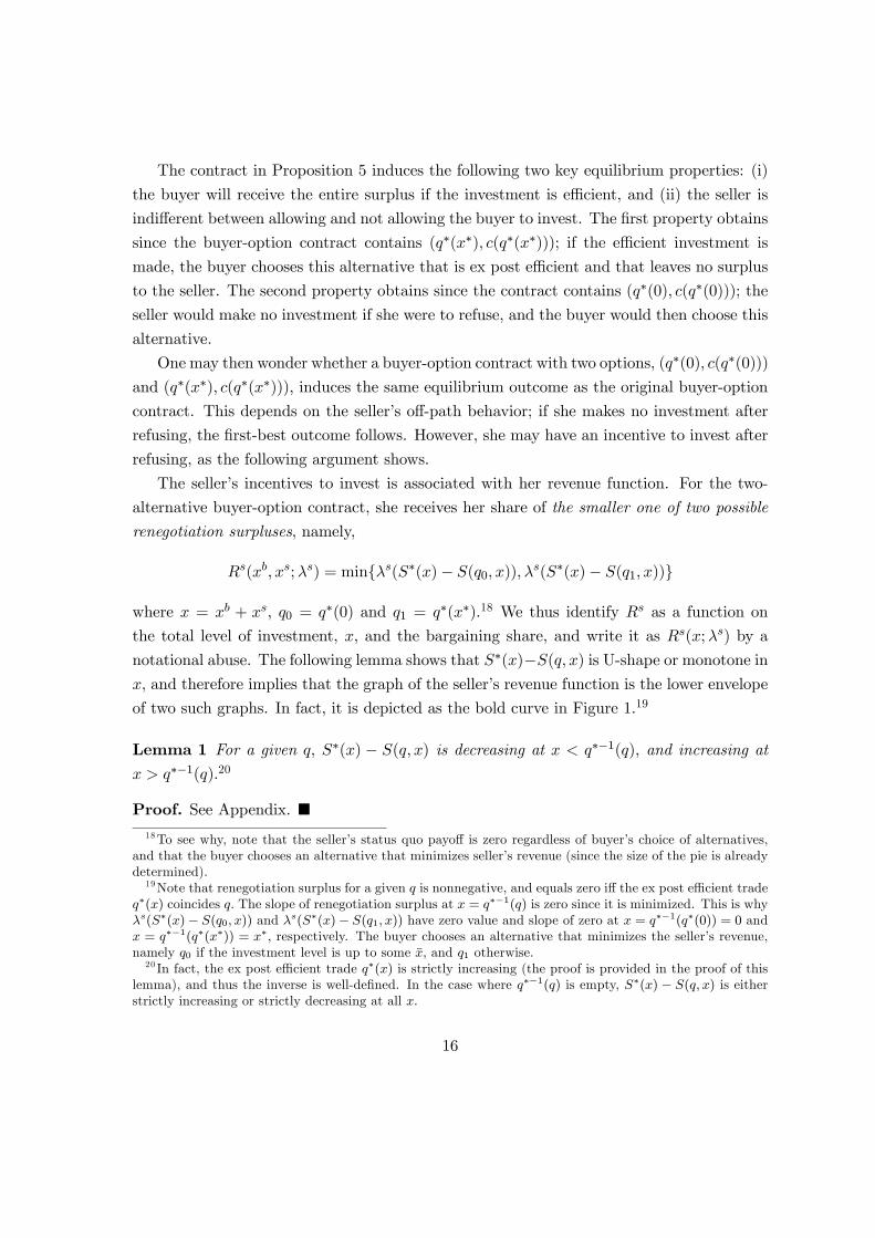
notational abuse. The following lemma shows that S∗(x)−S(q, x) is U-shape or monotone inx, and therefore implies that the graph of the seller’s revenue function is the lower envelope
of two such graphs. In fact, it is depicted as the bold curve in Figure 1.19
Lemma 1 For a given q, S∗(x) − S(q, x) is decreasing at x < q∗−1(q), and increasing atx > q∗−1(q).20
Proof. See Appendix. ¥18To see why, note that the seller’s status quo payoff is zero regardless of buyer’s choice of alternatives,
and that the buyer chooses an alternative that minimizes seller’s revenue (since the size of the pie is alreadydetermined).19Note that renegotiation surplus for a given q is nonnegative, and equals zero iff the ex post efficient trade
q∗(x) coincides q. The slope of renegotiation surplus at x = q∗−1(q) is zero since it is minimized. This is whyλs(S∗(x)− S(q0, x)) and λs(S∗(x)− S(q1, x)) have zero value and slope of zero at x = q∗−1(q∗(0)) = 0 andx = q∗−1(q∗(x∗)) = x∗, respectively. The buyer chooses an alternative that minimizes the seller’s revenue,namely q0 if the investment level is up to some x̄, and q1 otherwise.20 In fact, the ex post efficient trade q∗(x) is strictly increasing (the proof is provided in the proof of this
lemma), and thus the inverse is well-defined. In the case where q∗−1(q) is empty, S∗(x) − S(q, x) is eitherstrictly increasing or strictly decreasing at all x.
16

x
)),()(( * xqSxSs −λ
*xx
Figure 1:
The question is whether an investment level x0 exists such that making this investmentby her own provides positive surplus to her, i.e., Rs(x0;λs)−x0 > 0. If so, the seller optimallyrefuses to allow the buyer to invest. Whether such x0 exists depends on the seller’s bargainingshare λs. If the share is close enough to zero, the revenue function is so flat that no such x0
exists. Accordingly, define
λ̄s= max{λs ∈ (0, 1]|Rs(xs;λs)− xs ≤ 0 for all xs ≤ x∗}.21
If λs ≤ λ̄s, there is no x0 such that Rs(x0;λs)− x0 > 0. The above buyer-option contract of
two alternatives therefore induces the buyer to invest efficiently.
If λs > λ̄s, the contract does not work, but we can still construct another buyer-option
contract of finite alternatives that achieves the first-best. Consider adding another alterna-
tive (q = q∗(x), t = c(q∗(x))) for some x ∈ (0, x∗) to the two-alternative contract. The graphof the seller’s revenue function becomes the lower envelope of three graphs. Her revenue
becomes smaller, and her incentive to invest by her own must therefore be lowered. By
adding such alternatives for x = m/2n × x∗, m = 1, 2, ..., 2n − 1, her revenue function canbe arbitrarily close to zero in [0, x∗]. Adopting such a buyer-option contract, her incentiveto invest after refusing vanishes even when she has the entire bargaining power. We have
therefore established the following proposition:
Proposition 6 In the purely cooperative case, a buyer-option contract of finite alternativesexists which induces the buyer to invest at the first-best. If λs ≤ λ̄
s, the following buyer-
option contract achieves the first-best: {(q = q∗(x), t = c(q∗(x))) for x ∈ {0, x∗}}.21Note that if x > x∗, Rs(x;λs)− x ≤ 0 for any λs ≤ 1. Thus we do not need to look at x > x∗.
17
Uncertainty Uncertainty is beyond the scope of our analysis, but indeed the buyer-
option contract in Proposition 5 works under some types of uncertainty. Suppose that
there is a stochastic shock that only affects the buyer’s valuation. For example, uncertainty
affects the price of final goods that this buyer eventually supplies. The shock is realized
after investing but before the mechanism is played. Since the seller’s cost function is exactly
the same as before, the logic in Proposition 5 remains valid, and the full efficiency result
holds as well.
Corollary 1 In the purely cooperative case, suppose there is uncertainty that only affects thebuyer’s valuation. Then, the buyer-option contract of Proposition 5 achieves full efficiency.
6 Hybrid Cases — An Example
To investigate how contracting improves efficiency in hybrid cases, we first look at a specific
example in this section. A generalization follows in the next section.
Let the buyer’s valuation and the seller’s cost be, respectively,
v(q, x) = 4(1 + αx14 )q
c(q, x) = 4(1− (1− α)x14 )q + 2q2
where α ∈ [0, 1]. The parameter α measures cooperativeness of the investment. The condi-tion α = 0 corresponds to the purely selfish case, α = 1 the purely cooperative case, and
α ∈ (0, 1) a hybrid case. The associated functions and values are
S(q, x) = 4x14 q − 2q2
q∗ (x) = x14 ,
S∗(x) = 2x12
x∗ = 1,
The buyer’s and the seller’s interim payoffs are as follows:
rb(q0, x)− t0 = 2λbx12 + 4(α− λb)q0x
14 + 2λb(q0)2 − t0,
rs(q0, x) + t0 = 2λsx12 − 4(α− λb)q0x
14 − 2λb(q0)2 + t0,
where q0 and t0 are the chosen terms of a transaction in the message game.
18
To grasp a rough idea of how contracting affects the parties’ incentives to invest, consider
a noncontingent contract (q, t). The ex ante revenue functions given this contract are
Rb(xb, xs) = 2λb(xb + xs)12 + 4(α− λb)q(xb + xs)
14 + 2λb(q)2 − t, (3)
Rs(xb, xs) = 2λs(xb + xs)12 − 4(α− λb)q(xb + xs)
14 − 2λb(q)2 + t. (4)
The contract affects the parties’ incentives only through the second terms of the right-hand
sides in (3) and (4). The incentive effect of contracting thus depends not only on the
degree of cooperativeness, α, but also on the allocation of bargaining shares, λb and λs. For
example, suppose α− λb > 0. The buyer’s incentive to invest improves as q increases. This
observation suggests that the effect of a contract depends on the degree of cooperativeness
α relative to the buyer’s bargaining share, λb.
It should be mentioned that the revenue functions (3) and (4) are functions of the total
investment x = xb + xs for a noncontingent contract. We henceforth use Rb(x) and Rs(x)
for the parties’ revenue functions for a noncontingent contract.
Efficient Noncontingent Contracts for Highly Selfish Investment Consider the
case in which the investment is highly selfish relative to the buyer’s bargaining share. In
particular, suppose,22
α− λb ≤ − λb
qmax(5)
⇐⇒ λb ≥ αqmax
qmax − 1 ≡ α.
Suppose the parties adopt a noncontingent contract¡q, t¢for which
q = −λb/³α− λb
´≤ qmax.
The seller’s ex ante revenue given this contract is
Rs(x) = 2λsx12 + 4λbx
14 + constant,
which is strictly concave in x. The seller’s marginal revenue at x∗ = 1 is
Rs0(1) = λs (1)−1/2 + λb (1)−3/4 = 1
so that the seller has the right incentive to invest at the first-best level. This shows that if
(5) holds, the noncontingent contract (q, t) achieves full efficiency. Note that for the purely
selfish case, α = 0, (5) holds for all λb. This case corresponds to the result of Edlin and
Reichelstein (1996).22Recall that qmax is the upper bound of quantity traded. In this specific example, qmax > 1 must hold in
order to have interior solutions for the values such as q∗ and x∗.
19

Efficient Option Contracts for Highly Cooperative Investment We consider the
case in which the investment is highly cooperative and derive a contract that achieves full
efficiency. As one might expect from Proposition 4, we need to consider a more complex
contract than a noncontingent one. In this subsection, we look at a buyer-option contract
(q(x), t(x)) where the buyer reports a total investment level, x.
We use an analogy to the standard screening model (see, Mussa and Rosen (1978),
Maskin and Riley (1984)). Consider an agent with private information x (= xb + xs)
and a principal who does not know this agent’s type. The agent has a quasilinear utility
rb(q, x) − t where q is the quantity traded and t is the monetary transfer. The following
result is well-known: under the single-crossing property rbqx > 0, a mechanism (q(x), t(x))
is incentive compatible (i.e., the agent of type x0 optimally chooses the designated pair(q = q(x0), t = t(x0)) among the alternatives) if and only if q (x) is nondecreasing and for
all x0,
Rb¡x0¢ ≡ rb(q
¡x0¢, x0)− t
¡x0¢
= Rb(0) +
Z x0
0rbx(q(τ), τ)dτ.
The last integral equation is called the Mirrlees condition. The transfer function is defined
implicitly in the Mirrlees condition.
If we translate the agent into the buyer, and the principal into the court or the enforcer
of the contract, the above argument simply shows that the mechanism (q(x), t(x)) is a
buyer-option contract that induces the buyer’s revenue function, Rb(x). Note that it is a
function of the total investment x = xb + xs, not a function of (xb, xs).
If α− λb > 0, by (3) the single-crossing property rbqx > 0 holds. Define
q(x) = min
(1− λb
α− λbx14 , qmax
).
This is nondecreasing and thus if t(x) is defined through the Mirrlees condition, a buyer-
option contract (q(x), t(x)) is incentive compatible.
Suppose the parties adopt the buyer-option contract, (q(x), t(x)). The Mirrlees condition
gives the derivatives of the buyer’s ex ante revenue; for x0 such that q(x0) < qmax,
Rb0 ¡x0¢ = rbx(q(x0), x0)
= λbx0−12 + (α− λb)q
¡x0¢x0−
34
= λbx0−1
2 + (1− λb)x0−12
= S∗0(x0),
20
α α α 10bλ
Full efficiency achievable with subsidization
Full efficiency achievable without subsidization
Figure 2:
and similarly for x0 such that q(x0) = qmax,
Rb0(x0) ≤ S∗0(x0).
Suppose the investment is highly cooperative relative to λb to satisfy
α− λb ≥ (1− λb)/qmax (6)
⇐⇒ λb ≤ αqmax − 1qmax − 1 ≡ α.
Then
q(1) = min
(1− λb
α− λb, qmax
)≤ qmax
q (x) < qmax for x < x∗ = 1.
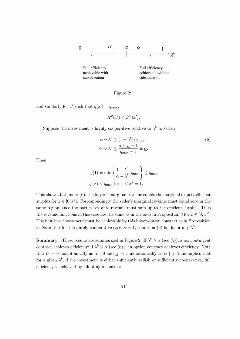
This shows that under (6), the buyer’s marginal revenue equals the marginal ex post efficient
surplus for x ∈ [0, x∗]. Correspondingly the seller’s marginal revenue must equal zero in thesame region since the parties’ ex ante revenue must sum up to the efficient surplus. Thus
the revenue functions in this case are the same as in the ones in Proposition 3 for x ∈ [0, x∗].The first-best investment must be achievable by this buyer-option contract as in Proposition
3. Note that for the purely cooperative case, α = 1, condition (6) holds for any λb.
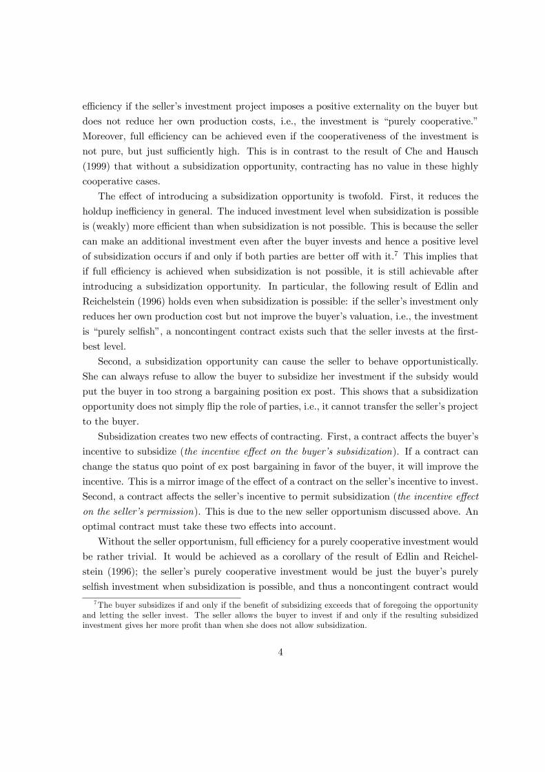
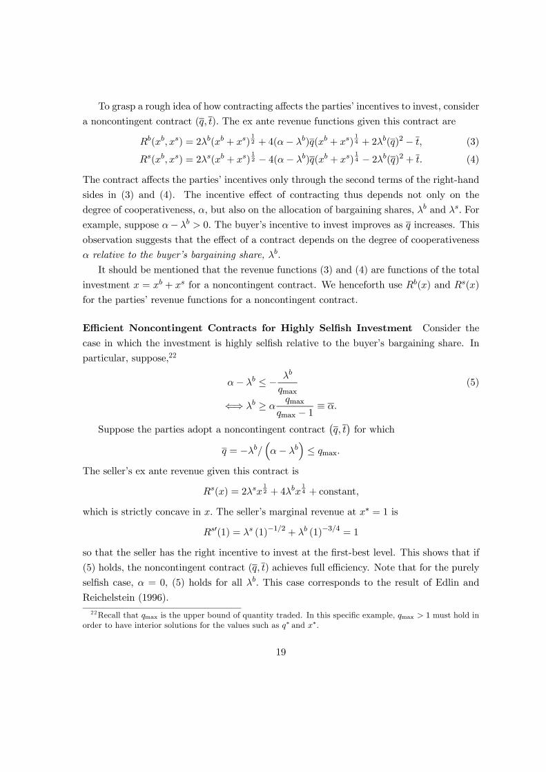
Summary These results are summarized in Figure 2. If λb ≥ α (see (5)), a noncontingent
contract achieves efficiency; if λb ≤ α (see (6)), an option contract achieves efficiency. Note
that α → 0 monotonically as α ↓ 0 and α → 1 monotonically as α ↑ 1. This implies thatfor a given λb, if the investment is either sufficiently selfish or sufficiently cooperative, full
efficiency is achieved by adopting a contract.
21
If α < λb < α, i.e., the degree of cooperativeness is intermediate, the two contracts
considered above do not achieve efficiency.23 However, the interval (α,α) becomes smaller
as qmax increases, and if we allow qmax =∞, there remains only one point, α = λb, at which
efficiency is unattainable.24
7 General Hybrid Cases
The example of the previous section suggests that in a more general setting, full efficiency
should be achievable for a hybrid case that is close to either of the two polar cases. In this
section, we give conditions for a hybrid case under which full efficiency can be achieved.
Two new issues arise in a general setting. First we need a measure of cooperativeness of
the investment analogous to α, α, and α in the example. Second, a noncontingent or option
contract may not achieve efficiency and we may need to use a general message game for an
optimal contract.
The second issue involves two analytical problems. The first problem is to specify the
set of feasible contracts. However, the revelation principle applies so that without loss of
generality, we restrict attention to direct mechanisms. The second problem is to derive
the ex ante revenues from a direct mechanism. It is extremely cumbersome to derive them
directly. However, Segal and Whinston (2002) provide a characterization result for feasible
ex ante revenues and we use this result.
We discuss these two problems in detail before analyzing the general hybrid cases.
“The Revelation Principle” Recall that the state space of the message game is the
set of investment pairs, {(xb, xs)}. The revelation principle implies that we can take eachparty’s message to be the investment pair that s/he has observed. However, in the present
context, a stronger result holds. The next proposition shows that each party’s message just
needs to be a report of the total investment level, x = xb + xs.
Proposition 7 Given any message game, the induced buyer’s and seller’s ex ante revenuefunctions satisfy Rb(xb, xs) = R̃b(x) and Rs(xb, xs) = R̃s(x). Moreover, there exists a
message game in which each party truthfully reports the total investment level, x, such that
23 In fact, we can show that full efficiency is not achievable by any contract in this case.24Sufficiency of the Mirrlees condition does not require compactness of the domain of the primitive func-
tions.
22
the same revenue functions R̃b(x) and R̃s(x) are induced.25 ,26
Proof. Consider a message game©q(mb,ms), t(mb,ms)
ªwith arbitrary message spaces,
M i, i = b, s. Given an investment pair (xb, xs), the payoff functions of this message game
are (see (1) and (2))
rb(q(mb,ms), xb + xs)− t(mb,ms) for the buyer,
rs(q(mb,ms), xb + xs) + t(mb,ms) for the seller.
Let (mb∗(xb, xs),ms∗(xb, xs)) denote a Nash equilibrium of the message game given the
investment pair (xb, xs). Recall that the message game is a two-person zero-sum game. The
parties’ equilibrium payoffs are thus the minimax values.
Consider another investment pair (xb0, xs0) such that xb + xs = xb0 + xs0. The payofffunctions given this new investment pair (xb0, xs0) are clearly the same as those given theold investment pair (xb, xs). The resulting equilibrium payoffs must be the same minimax
values even if the equilibrium strategy profile might be different. This shows that if xb+xs =
xb0 + xs0 = x,
Rb(xb, xs) = Rb(xb0, xs0) ≡ R̃b(x),
Rs(xb, xs) = Rs(xb0, xs0) ≡ R̃s(x).
In order to construct the desired mechanism, it is convenient to define the following
mapping: x 7→ ψ(x) = (xb, xs) for some (xb, xs) such that xb + xs = x. This ψ(x) gives a
representative investment pair, (xb, xs), for each total investment level, x.
Consider the following message game©q̃¡m̃b, m̃s
¢, t̃¡m̃b, m̃s
¢ªwith a message space
M̃ i = [0, xmax], i = b, s such that
q̃(x, x0) = q(mb∗(ψ(x)),ms∗(ψ(x0))),
t̃(x, x0) = t(mb∗(ψ(x)),ms∗(ψ(x0))).
If both parties report the true total investment level, each party receives its minimax pay-
off of the original game. Suppose one party deviates from reporting the true level. By
construction of this message game and the definition of the minimax value, the deviating
party must receive less than the minimax payoff of the original game. Truth-reporting is
25This proposition can be generalized. Suppose that the payoff-relevant variable for the message game issome aggregate value φ(x1, ..., xn) for a state (x1, ..., xn). In this case we can restrict attention to the messagegame in which each party announces φ.26Segal and Whinston (2002, p. 19) make a similar observation.
23
therefore a Nash equilibrium of this new message game. The induced revenue functions
must be R̃b(x) and R̃s(x). ¥
We henceforth assume that the messages are reports of x, and that the contract is
incentive compatible. The parties can anticipate the equilibrium outcome {q (x, x) , t (x, x)}for each x, and the buyer’s and the seller’s ex ante revenues are thus redefined as
Rb (x) = rb (q (x, x) , x)− t (x, x) ,
Rs (x) = rs (q (x, x) , x) + t (x, x) .
We call arbitrary revenue functions Rb (x) and Rs (x) implementable if there is an in-
centive compatible contract that generates them.
Segal-Whinston’s Characterization Segal and Whinston (2002) derive a characteri-
zation result for implementable utility mappings in mechanism design with renegotiation.
It can be applied to characterize implementable revenue functions in our model.
Definition 1 The buyer’s interim payoff rb satisfies the single-crossing property (SCP) if
either rbqx ≥ 0 or rbqx ≤ 0 in the entire domain.
If rb satisfies SCP, the seller’s interim payoff, rs, also satisfies the corresponding SCP.
This is because, rb(q, x) + rs(q, x) = S∗(x) for all (q, x) by ex post efficient renegotiation,which implies rbqx = −rsqx for all (q, x).We henceforth omit the labels “the buyer’s” or “theseller’s” when we refer the single-crossing property.
Lemma 2 (Segal-Whinston) Under the single-crossing property, ex ante revenue functionsRb (x) and Rs (x) are implementable iff, there is a function g : [0, xmax] → [0, qmax] such
that for any x0,
Rb(x0) = Rb (0) +
Z x0
0
∂rb (g (τ) , τ)
∂xdτ ,
Rs¡x0¢= Rs (0) +
Z x0
0
∂rs (g (τ) , τ)
∂xdτ.
We call this g(x) a generating decision rule.27,28
27 In their original version, a condition that is weaker than the single-crossing property, “Condition ±,”suffices to establish the result. From the maintained assumptions in our model, it is harder to check ifCondition ± holds than the single-crossing property. The single-crossing property holds in highly selfish andcooperative cases, as we show below.28Two differences between this lemma and the result for screening should be mentioned. The first one
24

This lemma says that for any contract, there is a corresponding decision rule that
generates the ex ante revenue functions induced by the contract. Conversely, for any decision
rule that generates Rb and Rs, there is a corresponding contract that induces the revenue
functions.
An advantage of using this lemma is in taking the derivatives of the revenue functions,
which represent the parties’ incentives to invest. Consider a generating decision rule g(x).
The Mirrlees condition implies
Rb0 (x) =∂rb (g (x) , x)
∂x= λbS∗0(x) + λsvx (g (x) , x) + λbcx (g (x) , x) a.e.
Rs0 (x) =∂rs (g (x) , x)
∂x= λsS∗0(x)− λsvx (g (x) , x)− λbcx (g (x) , x) a.e.
The last two terms in each line capture the effect of a contract on the party’s incentive to
invest. Note that the null contract corresponds to g (x) ≡ 0 and with it these two terms arezero.
The interpretation of the single-crossing property, rbqx > 0, is as follows: consider a
noncontingent contract (q, t). The buyer’s ex ante revenue function is then
Rb(x) = rb(q, x)
= v(q, x)− t+ λb[S∗(x)− S(q, x)]
= λbS∗(x) + λsv(q, x) + λbc(q, x)− t.
The marginal revenue of investment is
Rb0(x) = λbS∗0(x) + λsvx(q, x) + λbcx(q, x)
Suppose the single-crossing property rbqx > 0 holds, i.e.,
λsvqx(q, x) + λbcqx(q, x) > 0.
Then increasing the trade quantity q will improve the buyer’s incentive to invest.
lies in the restriction to the generating decision rule. In screening, the generating rule must be monotonicwhereas it is arbitrary in mechanism design with renegotiation. This is explained by the fact that theinformation extracted from the message game is richer than that from the option contract. In screening,only one agent with private information reports a message. This is an option contract. In mechanism designwith renegotiation, two parties who share information report messages.Another difference is in the role of the generating decision rule. In screening, the rule coincides with the
equilibrium decision rule. In mechanism design with renegotiation, it need not, due to renegotiation. SeeSegal and Whinston (2002, p.11).
25

Two further remarks should be mentioned. First, it is typically complicated to construct
a contract that corresponds to some generating decision rule g. See Segal and Whinston
(2002) for a construction. The contract has a simple form only in special cases. For example,
it is a noncontingent contract (q, t) if and only if g(x) = q. If rbqx > 0, it is a buyer-option
contract if and only if g(x) is nondecreasing. Second, the single-crossing condition may
not hold in the general case. It depends on the primitive functions and the allocation of
bargaining shares. We will find conditions under which it holds.
7.1 Efficiency in Highly Cooperative Cases
We prove that full efficiency can be achieved if the investment is sufficiently cooperative.
We use Segal-Whinston’s lemma to find a contract to be adopted. Since the single-crossing
property may not always hold, we need to give a condition for it. To state and prove the
result, we define a measure of cooperativeness.
To give a condition for the single-crossing property, define the following measure:
αc = sup{k ∈ [0, 1]|(1− k)vqx (q, x) + kcqx (q, x) > 0 ∀(q, x)},
and αc = 0 if there is no such k. It is straightforward that the single-crossing property holds
if λb < αc. This shows that Segal-Whinston’s lemma is more likely to apply as αc increases.
For a purely cooperative investment, the cross derivative cqx ≡ 0 so that αc = 1. For the
example of section 6, αc = α.
We measure cooperativeness of the investment as follows:
α∗c = sup½k ∈ [0, αc]
¯̄̄̄(1− k)vx (qmax, x) + kcx (qmax, x)≥ (1− k)S∗0(x) ∀x ∈ [0, x∗]
¾, (7)
and α∗c = 0 if there is no such k.29 Note that by construction (k ∈ [0, αc]) α∗c ≤ αc.30 For
the example of section 6, α∗c = α.
To justify this α∗c as a measure of cooperativeness, consider a purely cooperative invest-ment first, i.e., cx ≡ 0. For all x,
(1− k)vx (qmax, x) + kcx (qmax, x)
= (1− k)vx (qmax, x) by pure cooperativeness
≥ (1− k)vx(q∗(x), x)by complementarity and qmax ≥ q∗(x)
= (1− k)S∗0(x) by the envelope theorem.29Che and Hausch (1999) similarly define measures of cooperativeness.30The inequality in (7) can be satisfied for k > αc for some v and c.We restrict our attention to αc > k = λb
since otherwise we cannot use Segal-Whinston’s characterization lemma.
26

This shows α∗c = 1. For a hybrid case, if α∗c is high, |cx| must be small relative to |vx| sothat the investment must be highly cooperative. For a purely selfish investment, it is clear
that α∗c = 0.To get an intuition for the inequality condition in (7), consider a noncontingent contract.
Recall that λbvx + λscx measures the incentive effect of the contract. Under the single-
crossing condition (assured by λb < αc), the left-hand side in (7) measures the maximum
effect of a noncontingent contract on the buyer’s incentive to invest. The right-hand side is
the buyer’s incentive loss due to hold up given the null contract. Thus this condition says
that a noncontingent contract can adequately make up for the incentive loss due to holdup,
for the buyer.
With this measure, we prove the following result.
Proposition 8 Suppose α∗c > λb holds. Then a contract exists which induces the buyer to
entirely invest at the first-best investment level in a subgame perfect equilibrium.
Proof. See Appendix. ¥
As in Proposition 5, one way to achieve full efficiency is to solve the following two prob-
lems simultaneously: giving the right incentive to invest to the buyer and giving the right
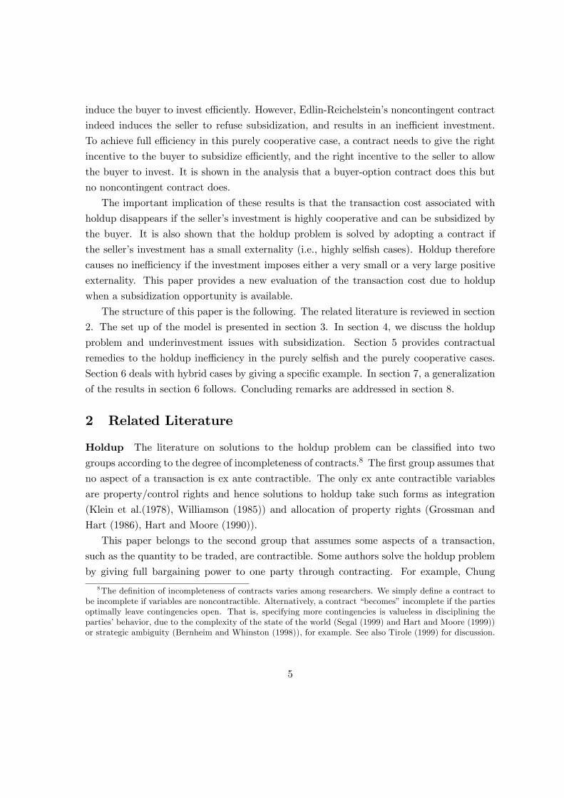
incentive to permit subsidization to the seller. If, as depicted in Figure 3, buyer’s marginal
revenue of investment equals the marginal ex post efficient surplus by adopting a contract,
corresponding seller’s marginal revenue must be zero, and the two problems are therefore
solved. Under the assumption in Proposition 8, we have seen that a noncontingent contract
can adequately make up for the incentive loss due to holdup. However, a noncontingent con-
tract might be too blunt to pinpoint the marginal revenues. In such a case, the proposition
assures that a more complex contract works to adjust the revenues.
Che and Hausch (1999) show that when investment is highly cooperative, the null con-
tract is optimal. Using the next proposition, we can compare the result of Che and Hausch
with Proposition 8.
Proposition 9 Suppose αc > λb holds. Then, without a subsidization opportunity, the null
contract is optimal (hence contracting has no value).
Proof: See Appendix. ¥
This proposition implies the following: if the investment is cooperative enough to achieve
efficiency (α∗c > λb, by Proposition 8), contracting indeed has no value without a subsidiza-
tion opportunity (αc ≥ α∗c > λb, by Proposition 9).
27

1
)('* xS
*x
)('* xSbλ
)('* xSsλ
1
*x
)(' xRb
)(' xRs
Figure 3:
The intuition of Proposition 9 is as follows. Recall that when the single-crossing property
holds, every noncontingent contract improves only the buyer’s incentive to invest. Since the
message game is zero-sum, contracting only impairs the seller’s incentive to invest. When
subsidization is not possible, the seller’s incentive to invest should be maximized so that
the null contract is optimal.
7.2 Efficiency in Highly Selfish Cases
We prove that full efficiency can be achieved if the investment is sufficiently selfish. The logic
is parallel to that in the last subsection. Subsidization does not occur in equilibrium, and
thus this analysis also applies to the case when subsidization is not possible. We compare
this result with existing results at the end of this subsection.
To give a condition for the other single-crossing property, rbqz < 0, define the following
measure:
αs = inf{k ∈ [0, 1]|(1− k)vqx (q, x) + kcqx (q, x) < 0 ∀(q, x)},and αs = 1 if there is no such k. The single-crossing property, rbqx < 0, holds if αs < λb.
Note that for a purely selfish investment, αs = 0, and also that αc ≤ αs by definition. In
the previous example, αs = α.
We measure cooperativeness of the investment in an alternative way:
α∗s = inf½k ∈ [αs, 1]
¯̄̄̄ −(1− k)vx (qmax, x)− kcx (qmax, x)≥ kS∗0(x) ∀x ∈ [0, x∗]
¾,
28
and α∗s = 1 if there is no such k. As in the last subsection, we can show that if the investmentis purely selfish, α∗s = 0. For a hybrid case, if α∗s is low, |cx| must be large relative to |vx|so the investment must be highly selfish. For a purely cooperative investment, it is clear
that α∗c = 1. These arguments justify that α∗s measures cooperativeness of the investment.In the previous example, α∗s = α. Note that α∗s ≥ αs by definition.
Following the same logic as in the highly cooperative case, we can derive a contract
such that full efficiency is achieved for a sufficiently highly selfish investment. The derived
contract is a message game {q(·, ·), t(·, ·)}. Applying Proposition 9 in Segal and Whinston(2002), we can derive a buyer-option contract that achieves the equilibrium outcome of the
original message game.31
Proposition 10 Suppose α∗s < λb. Then a buyer-option contract exists such that the seller
invests entirely at the first-best level in a subgame perfect equilibrium. Subsidization does
not occur in equilibrium.
Che and Hausch (1999) and Segal and Whinston (2002) derive a first-best noncontingent
contract for highly selfish cases if the seller’s ex ante payoff Rs(x) − xs is strictly concave
for any noncontingent contract. This condition may not hold in general and hence in
our setting, a more complex contract may be necessary. This result does not contradict
Che-Hausch-Segal-Whinston’s result since a buyer-option contract can be a noncontingent
contract.
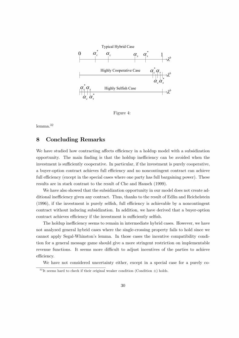
7.3 Summary
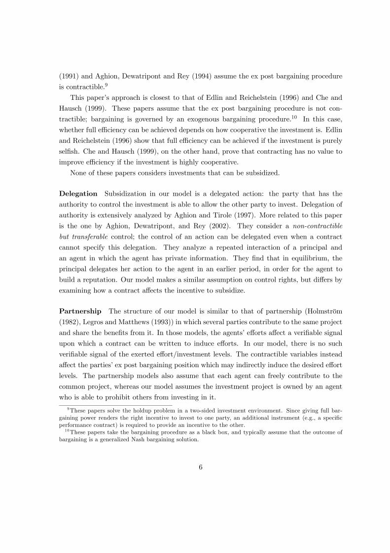
For general hybrid cases, the level of each party’s bargaining power affects whether adopting
a contract can achieve full efficiency. Given a hybrid investment, the weaker the buyer’s
bargaining power, the more likely full efficiency via subsidization is available. Similarly, the
stronger the buyer’s bargaining power, the more likely full efficiency via non-subsidization
is available. Which of those efficiency results are more available depends on the measures
of cooperativeness (Figure 4).
When αc < λb < αs, we can not say much about optimal contracts, since the single-
crossing property does not hold within this region, and we can not use Segal-Whinston’s
31The buyer-option contract is constructed as follows: for a given message game, create a new contract byrestricting the seller’s message only to the equilibrium message when the efficient investment is made. Thenew contract is a buyer-option contract. By adopting this contract, the seller invests efficiently; her payoffremains the same if she invests efficiently but (weakly) decreases if she invests at a different level because ofthe zero-sum nature of the game.
29
*sα
*cα cα sα
*sα 10
*cα
cα
sα*sα
*cα
cαsα Highly Selfish Case
Highly Cooperative Case
Typical Hybrid Case
bλ
bλ
bλ
Figure 4:
lemma.32
8 Concluding Remarks
We have studied how contracting affects efficiency in a holdup model with a subsidization
opportunity. The main finding is that the holdup inefficiency can be avoided when the
investment is sufficiently cooperative. In particular, if the investment is purely cooperative,
a buyer-option contract achieves full efficiency and no noncontingent contract can achieve
full efficiency (except in the special cases where one party has full bargaining power). These
results are in stark contrast to the result of Che and Hausch (1999).
We have also showed that the subsidization opportunity in our model does not create ad-
ditional inefficiency given any contract. Thus, thanks to the result of Edlin and Reichelstein
(1996), if the investment is purely selfish, full efficiency is achievable by a noncontingent
contract without inducing subsidization. In addition, we have derived that a buyer-option
contract achieves efficiency if the investment is sufficiently selfish.
The holdup inefficiency seems to remain in intermediate hybrid cases. However, we have
not analyzed general hybrid cases where the single-crossing property fails to hold since we
cannot apply Segal-Whinston’s lemma. In those cases the incentive compatibility condi-
tion for a general message game should give a more stringent restriction on implementable
revenue functions. It seems more difficult to adjust incentives of the parties to achieve
efficiency.
We have not considered uncertainty either, except in a special case for a purely co-
32 It seems hard to check if their original weaker condition (Condition ±) holds.
30

operative investment. Uncertainty creates another holdup problem that complicates the
investment incentives. Our approach separates the holdup problem due to uncertainty from
the one due to relationship-specific investment. Including uncertainty causes a big analytical
problem: Segal-Whinston’s lemma cannot apply unless information about the multidimen-
sional state space is aggregated into a single number. Future research should explore how
to characterize an optimal or efficient contract in cases with a multidimensional state space.
Despite restricting assumptions, we have seen that a subsidization opportunity improves
contractual solutions to the holdup problem in the cases that have been thought of as
impossible to remedy (e.g., highly cooperative cases). Introducing subsidization would shed
light on the firm’s cooperative behavior in making relationship-specific investments and on
the firm’s decision about integration. To combine repeated interaction and reputation with
subsidization might be fruitful to understand the firms’ dynamic decision making regarding
their behavioral and organizational choice. This issue is left for future research.
A Appendix
Proof of Proposition 4. By Proposition 1, when either party has full bargaining power,the first-best investment is achieved. Suppose then each party has a positive bargaining
share and there is a noncontingent contract¡q, t¢that will induce x∗.
First, we show that this contract must induce the buyer to entirely invest x∗. Supposeon the contrary the seller invests xs ∈ (0, x∗]. The seller’s revenue is
Rs(xb, xs) = t− c (q) + λs[S∗(xb + xs)− S³q, xb + xs
´]
≡ R̃s(xb + xs).
(Note that for a noncontingent contract, the revenues only depend on the total investment
given xb and xs). Since the seller invests after the buyer,
dRs
dxs(xb, xs) =
∂Rs
∂xs(xb, xs)
= R̃s0(x∗)
= λs[S∗0(x∗)− Sx(q, x∗)]
= λs[1− vx(q, x∗)]
< 1.
This is a contradiction since the seller’s marginal revenue must equal to 1. Thus the buyer
invests all the efficient investment.
31

Next, we show that q = q∗(x∗). Recall first that the buyer’s revenue given (xb, xs) is
Rb(xb, xs) = v(q, xb + xs)− t+ λb[S∗(xb + xs)− S³q, xb + xs
´]
≡ R̃b(xb + xs).
Since the buyer chooses xb = x∗ in equilibrium, his marginal revenue dRb/dxb at (x∗, 0)must be 1, the marginal cost. To derive the expression of dRb/dxb, he needs to anticipate
the seller’s response xs(xb). However, we have seen that
dRs
dxs(x∗, 0) < 1,
and by continuity,dRs
dxs(x∗ + ε, 0) < 1 for small ε > 0. This shows xs0(x∗) = 0. Thus,
dRb
dxb(x∗, xs(x∗)) =
∂Rb
∂xb(x∗, 0)
= R̃b0(x∗).
This implies R̃b0(x∗) = S∗0 (x∗) = 1. Notice that R̃b(x) + R̃s (x) ≡ S∗(x).This implies
R̃s0(x∗) = S∗0(x∗)− R̃b0(x∗) = 0
=⇒ λs[S∗0(x∗)− Sx(q, x∗)] = 0
=⇒ λs[S0x(q∗(x∗), x∗)− Sx(q, x
∗)] = 0 by the envelope theorem
=⇒ q = q∗ (x∗) by Sqx = vqx > 0.
This shows q = q∗(x∗).Therefore, this noncontingent contract induces no renegotiation on the equilibrium path.
Now suppose that the seller refuses to allow the buyer to invest and does not invest
afterwards. The resulting total investment level is zero and the seller’s payoff is
t− c(q) + λs[S∗(0)− S(q, 0)]. (8)
The renegotiation surplus must be positive since q∗(0) 6= q∗(x∗) = q.33 However, the seller’s
payoff on the equilibrium path equals to the status quo payoff with no renegotiation surplus,
which is strictly less than the one in (8). This is a contradiction. ¥
Proof of Lemma 1. First, we show that q∗ is strictly increasing. The ex-post efficienttrade q∗(x) is defined implicitly by
vq (q∗ (x) , x)− cq (q
∗ (x) , x) = 0.33Strict monotonicity of q∗ is proved in the proof of Lemma 1.
32

By the implicit function theorem,
q∗0(x) = −vqx(q∗ (x) , x)− cqx (q
∗ (x) , x)vqq (q∗ (x) , x)− cqq (q∗ (x) , x)
> 0.
Recall that the ex post efficient surplus S∗(x) is differentiable, and by the envelopetheorem, S∗0(x) = vx (q
∗ (x) , x)− cx (q∗ (x) , x) . Now,
S∗0 (x)− Sx (q, x) = [vx (q∗ (x) , x)− cx (q
∗ (x) , x)]− [vx (q, x)− cx (q, x)]
= [vqx (q̃, x)− cqx (q̃, x)] (q∗ (x)− q)
for some q̃ between q∗ (x) and q (by the mean value theorem). The term in square brackets
in the second line is positive by assumption. Hence
S∗0(x)− Sx(q, x) T 0 iff q∗ (x) T q iff x T q∗−1 (q) .
In the case where q∗−1 (q) is not well-defined, replace it with 0 if q < q∗(0) or with +∞ if
q > q∗(x) for all x. ¥
Proof of Proposition 8. Since αc > λb, the single crossing property holds, and Lemma 2
thus applies. Note the following condition is always available by setting g(x) = 0;
λsvx (0, x) + λbcx (0, x) = 0.
The condition α∗c > λb implies
λsvx (qmax, x) + λbcx (qmax, x) ≥ λsS∗0(x) for ∀x ∈ [0, x∗].
By the intermediate value theorem, there is qe(x) for x ∈ [0, x∗] such that
λsvx (qe(x), x) + λbcx (q
e(x), x) = λsS∗0(x) for ∀x ∈ [0, x∗].
Define a generating decision rule as
g(x) =
½qe(x) for x ∈ [0, x∗],0 otherwise.
Then by adopting a contract corresponding to g, the buyer’s revenue satisfies
Rb0(x) =½
S∗0(x) for x ∈ [0, x∗],λbS∗0(x) otherwise.
The seller’s revenue satisfies
Rs0(x) =½0 for x ∈ [0, x∗],λsS∗0(x) otherwise.
33
Therefore, the buyer’s revenue function coincides with the ex post efficient surplus in
[0, x∗], and the seller’s revenue function is zero in the same region. By construction, thebuyer’s revenue is concave, and the seller will never have incentive to invest (i.e., Rs0(x) < 1for all x).With the same logic as in Proposition 5, the seller allows the buyer to invest, and
the buyer invests efficiently. ¥
Proof of Proposition 9. Since αc > λb, the single-crossing property rbqx > 0 holds.
This is equivalent to rsqx < 0. The seller’s marginal revenue given a contract is, for the
corresponding g(x),
Rs0 (x) = λsS∗0(x)− λsvx (g (x) , x)− λbcx (g (x) , x) a.e.
Recall that the null contract gives Rs0 (x) = λsS∗0(x), and by the single-crossing propertythe seller’s incentive decreases when g(x) is nonzero. Therefore, the null contract is optimal
when there is no subsidization opportunity. ¥
References
[1] Aghion, Philippe, Mathias Dewatripont, and Patrick Rey, “Renegotiation Design with
Unverifiable Information.” Econometrica, March 1994, 62(2), pp.257-82.
[2] Aghion, Philippe, Mathias Dewatripont, and Patrick Rey, “On Partial Contracting.”
European Economic Review, April 2002, 46(4-5), pp. 745-53.
[3] Aghion, Philippe and Jean Tirole, “Formal and Real Authority in Organizations.”
Journal of Political Economy, February 1997, 105, pp. 1-29.
[4] Asanuma, Banri, “Manufacturer-Supplier Relationships in Japan and the Concept of
Relation-Specific Skill.” Journal of the Japanese and International Economies, March
1989, 3(1), pp.1-30.
[5] Bernheim, B. Douglas, and Michael D. Whinston, “Incomplete Contracts and Strategic
Ambiguity.” American Economic Review, September 1998, 88(4), pp.902-932.
[6] Burt, David, “Managing Suppliers Up to Speed.” Harvard Business Review, July-
August 1989, pp.127-135.
[7] Che, Yeon-Koo, and Donald B. Hausch, “Cooperative Investment and the Value of
Contracting.” American Economic Review, June 1999, 89(1), pp.125-47.
34
[8] Chung, Tai-Yeong, “Incomplete Contracts, Specific Investment and Risk Sharing.”
Review of Economic Studies, October 1991, 58(5), pp. 1031-42.
[9] Coase, Ronald H., “The Nature of the Firm.” Economica, n.s., 1937, 4, pp. 386-405.
[10] Coase, Ronald H., “The Acquisition of Fisher Body by General Motors.” Journal of
Law and Economics, April 2000, 63, pp. 15-31.
[11] Edlin, Aaron, and Stefan Reichelstein, “Holdups, Standard Breach Remedies, and
Optimal Investment.” American Economic Review, June 1996, 86(3), pp.275-91.
[12] Grossman, Sanford, and Oliver Hart, “The Costs and Benefits of Ownership: A Theory
of Vertical and Lateral Integration.” Journal of Political Economy, August 1986, 94(4),
pp. 691-719.
[13] Hart, Oliver, Firms, Contracts, and Financial Structure, Oxford, Clarendon Press,
1995
[14] Hart, Oliver, and John Moore, “Incomplete Contracts and Renegotiation.” Economet-
rica, July 1988, 56(4), pp.755-85.
[15] Hart, Oliver and John Moore, “Property Rights and the Nature of the Firm.” Journal
of Political Economy, December 1990, 98(6), pp.1119-58.
[16] Hart, Oliver and John Moore, “Foundations of Incomplete Contracts” Review of Eco-
nomic Studies, January 1999, 66(1), pp. 115-138.
[17] Holmström, Bengt, “Moral Hazard in Teams.” Bell Journal of Economics, Autumn
1982, 13(2), pp. 324-40.
[18] Holmström, Bengt, and John Roberts, “The Boundaries of the Firm Revisited.” Jour-
nal of Economic Perspectives, Fall 1998, 12(4), pp73-94
[19] Klein, Benjamin, Robert G. Crawford, and Armen A. Alchian, “Vertical Integration,
Appropriable Rents, and the Competitive Contracting Process.” Journal of Law and
Economics, October 1978, 21(2), pp. 297-326.
[20] Legros, Patrick and Steven A. Matthews, “Efficient and Nearly-Efficient Partnerships.”
Review of Economic Studies, July 1993, 60(3), pp. 599-611.
[21] MacLeod, W. Bently and James Malcomson, “Investments, Hold-up, and the Form of
Market Contracts.” American Economic Review, September 1993, 83(4), pp.811-37.
35

[22] Maskin, Eric, and John Moore, “Implementation and Renegotiation.” Review of Eco-
nomic Studies, January 1999, 66(1), pp.39-56.
[23] Maskin, Eric, and John Riley, “Monopoly with Incomplete Information.” Rand Journal
of Economics, Summer 1984, 15 (2) pp. 171-96.
[24] Maskin, Eric, and Jean Tirole, “Unforeseen Contingencies and Incomplete Contracts.”
Review of Economic Studies, January 1999, 66(1), pp. 83-114.
[25] Mussa, Michael, and Sherwin Rosen, “Monopoly and Product Quality.” Journal of
Economic Theory, August 1978, 18 (2), pp. 301-17.
[26] Nöldeke, Georg, and Klaus Schmidt, “Option Contracts and Renegotiation: A Solution
to the Hold-Up Problem.” Rand Journal of Economics, Summer 1995, 26(2), pp.163-79.
[27] Segal, Ilya, “Complexity and Renegotiation: A Foundation for Incomplete Contracts.”
Review of Economic Studies, January 1999, 66(1), pp. 39-56.
[28] Segal, Ilya, and Michael Whinston, “The Mirrlees Approach to Mechanism Design
with Renegotiation (with Applications to Hold-up and Risk Sharing).” Econometrica,
January 2002, 70(1), pp.1-45.
[29] Tirole, Jean, “Incomplete Contracts: Where Do We stand?” Econometrica, July 1999,
67(4), pp.741-781.
[30] Williamson, Oliver E. The Economic Institutions of Capitalism, New York, Free Press,
1985.
36