arX

iv:h

ep-p

h/02

0906

8v1

6 S

ep 2

002

CERN-TH/2002-226

HISTORY OF SPIN AND STATISTICS

A. Martin

Theoretical Physics Division, CERNCH - 1211 Geneva 23

andLAPP, Chemin de Bellevue, F-74941 Annecy-le-Vieux

Abstract

These lectures were given in the framework of the “Dixieme seminaire rhodanien de physique”entitled “Le spin en physique”, given at Villa Gualino, Turin, March 2002. We have shownhow the difficulties of interpretation of atomic spectra led to the Pauli exclusion principle andto the notion of spin, and then described the following steps: the Pauli spin with 2×2 matricesafter the birth of “new” quantum mechanics, the Dirac equation and the magnetic moment ofthe electron, the spins and magnetic moments of other particles, proton, neutron and hyperons.Finally, we show the crucial role of statistics in the stability of the world.

CERN-TH/2002-226August 2002

BIBLIOGRAPHY

I. Most essential references

• S.I. Tomonaga, The Story of Spin, English translation by T.Oka, The University ofChicago Press, 1997.

• Theoretical Physics in the 20th Century, Pauli memorial volume, M. Fierz, V.F. Weisskopfeds., Interscience 1959.

• Max Born, Atomic Physics, 7th edition 1962, Blackie and Son, Glasgow.

II. Additional Material

• E. Chpolski, Physique Atomique, traduction francaise, Editions Mir 1978.

• F. Gesztesy, H. Grosse and B. Thaller, Phys. Rev. Letters 50 (1983) 625.

• W. Thirring, Lehrbuch der Mathematische Physik, Quanten Mechanik Grosser systeme(Springer 1980).

• H. Grosse and A. Martin, Particle Physics and the Schrodinger Equation, CambridgeUniversity Press, 1997.

1

1 Introduction

Before speaking of spin, I have to speak of angular momentum, and specifically classical angularmomentum. We know since a long time that angular momentum is a conserved quantity.Specifically one of Kepler’s laws of the motion of planets around the sun, the “law of areas” isnothing but the conservation of angular momentum:

If a planet moves around the sun, the time taken by the planet to go from 1 to 2 is equalto the time taken to go from 3 to 4 if the shaded areas, delimited by the trajectory and rayscoming from the sun, are equal.

S

21

3

4

Figure 1

The angular momentum of the planet is

~xΛ~p = m~xΛd~x

dt, (1)

its derivative with respect to time is

md

dt

[

~xΛd~x

dt

]

= md~x

dtΛd~x

dt+ ~xΛ

d2~x

dt2m . (2)

The first term is obviously zero. From Newton’s law for a central force

md2~x

dt2=~x

rF (r) ,where r = |~x| , (3)

and hence the second term in (2) is also zero. The angular momentum is a constant of motion,and this does not depend on the force behaving like r−2. However, ~xΛd~x represents preciselytwice the area spanned by the rays going from the sun to the planet during an interval dt.Hence the “area law” holds at the infinitesimal level.

Since Bohr’s model of the atom (1913) angular momentum was quantized

|~L| = ℓh/ , (4)

2

and, in addition, the projection of the angular momentum along the z axis, M was also quan-tized:

M = mh/ . (5)

The energy levels of atoms, especially Alcaline atoms (the first row of Mendeleieff’s classifica-tion) were characterized by n (principal quantum number) and ℓ (orbital angular momentum,called k by the pioneers – but I prefer to use the modern notation).

However, take the yellow light of Sodium, that light which illuminates tunnels and makesyou look like a corpse. With a rather ordinary spectrometer that first year students wereusing at the Ecole Normale Superieure when I was there, you discover that this 3P → 2S line(n = 3, ℓ = 1 to n = 2, ℓ = 0) is in fact a doublet, the relative spacing between the two linesbeing about 1/1000. This means that there is something wrong with the classification of energylevels and spectral lines.

2 The Pre-Spin, Pre-Quantum Mechanics Periods and

the Discovery of Spin

In first approximation, in the Bohr model, the energy levels of Hydrogen depended only onequantum number the “Principal quantum number”, n, as indicated on Fig. 2

n = 4n = 3n = 2

n = 1l = 0

l = 1l = 2

l = 3

S

PD

F

Figure 2

The energy levels were degenerate in ℓ, the orbital angular momentum.

In Alcaline atoms, with a single valence electron, the energy levels also depend on ℓ, in sucha way

n0 + 1

n0

n0 + 2n0 + 3

l = 0

l = 1

l = 2l = 3

Figure 3

3

that for a fixed principal quantum number, the energy increases as ℓ increases. This is outsidethe subject but let me say that the best, most rational explanation of this fact was only givenrelatively recently by Baumgartner, Grosse and myself [1]. It is due to the fact that the valenceelectron is submitted to the field of the nucleus which is pointlike at this scale and of the electroncloud which has a negative charge and hence produces a potential with negative laplacian.

The observed transitions between levels satisfy the rule |∆ℓ| = 1. However, in fact, as wealready mentioned it, the levels of the Alcaline atoms are doublets. Similarly, the levels of theAlcaline earths, with Magnesium as a prototype, with two valence electrons are either singletsor triplets. This is illustrated on Fig. 4.

Figure 4

Another important piece of the puzzle is the Zeeman effect: the splitting of the energy levelsinside a uniform magnetic field. In a weak magnetic field, one observes, in the case of Alcalineatoms, that except for the ℓ = 0 state which is a singlet, all other doublets, for ℓ 6= 0, splitin such a way that one member gives 2ℓ levels and the other 2ℓ + 2 levels. This could not beexplained by what was known at the time.

What could be explained was the so-called “NORMAL” Zeeman effect, according to whicha level with orbital angular momentum component m along the z axis would be shifted by amagnetic field H in the z direction by

∆E(n,m, ℓ) =eh/

2mcHm , (6)

eh/2mc

is called the Bohr magneton.

This is because an electron circulating around the atom is equivalent to a current producinga magnetic moment.

Similarly, in strong magnetic fields (the so-called Paschen-Back effect), what is seen is alsovery different. We also see more levels than we should. Both situations are illustrated on Fig. 5.

4

It is of course difficult to describe the difficulties of the pioneers seeing this, because we aresomehow like in a TV episode where we know already who is guilty, but inspector Columbodoes not know yet!

Among the main protagonists were Lande, Pauli and Sommerfeld. All of them realized thatan extra quantum number beside n, ℓ and m was needed. Their models fitted the data, butthey knew they were only models. They were called “ERSATZ” models. Those of you whohave lived in occupied Europe during the war know what an ersatz is. It is a bad substitutefor something much better. However, in this case, the ERSATZ was replacing something whichdid not exist yet.

Sommerfeld and Lande were putting the fourth quantum number in the “core” of the atomwithout a very precise definition of the core (nucleus? or nucleus plus inner electrons?). Thecore was carrying angular momentum, 1/2 in the case of the alcaline atoms, had a magneticmoment, twice what you get in the case orbital angular momentum: 2 × 1/2 × electron Bohrmagneton. That was in 1923.

Pauli did not like that, for many reasons. For instance, if you remove an electron from Mg,you get Mg+ which behaves like an Alcaline atom, except for the fact that it is not neutral.By miracle, the “core” which had angular momentum 0 or 1 suddenly gets angular momentum1/2.

Pauli, in early 1925, decided that an extra quantum number was a “classically undescribabletwo-valuedness” which belonged to the electron, and formulated his famous exclusive principle,according to which two electrons cannot be in the same state. With this principle you “explain”the filling of the successive shells. For instance, sodium is

You explain also the counting of levels in weak and strong magnetic fields as it is seen inFig. 5.

Pauli was not, however, willing to make the big jump that this is due to an intrinsic angularmomentum 1/2 h/ of the electron. It was R.L. Kronig, arriving in Germany from the U.S.who proposed this idea first. However, this idea was not well received by Pauli, as well as inCopenhagen where Kronig went visiting. There was also a problem about the spacing of thelevels which gave doubts to Kronig himself. Then in the fall of 1925, Uhlenbeck and Goudsmit,in Leiden, proposed the same idea which they sent for publication to Naturwissenshaften. Afterdiscussions with Lorentz, they tried to withdraw their paper, but it was too late (fortunately)and it was published!

Naturally the gyromagnetic factor of the electron was taken to be 2 to fit the experiment,so that the magnetic moment of the electron was 2 × 1/2 × 1 Bohr magneton.

There was a problem, however, which is that a naıve calculation of the energy interval in adoublet, due to the coupling of the orbital motion with the spin of the electron, gave a resulttwice too big as stressed by a letter of Kronig against the Uhlenbeck–Goudsmit hypothesis. Itwas G.H. Thomas who realized that relativistic effects in the motion of the electron shouldbe treated more carefully. It amounts to replacing g, the gyromagnetic factor of the electron,

5

which was empirically 2, by g − 1, i.e. 1. This is treated in the lectures of E. Leader and so Ishall not attempt to describe the reasoning of Thomas.

Before going to the true quantum mechanical situation, I would like to show to you how, inthe time of “old” quantum mechanics, people calculated the “Lande factor” giving the magneticsplittings in weak fields. The magnetic interaction is given by

W = − eh/

2mc〈Hµ′′

〉 (7)

where µ′′ is the projection of the total magnetic moment on the total angular momentum~L+ ~S = ~J ;

µ′′ =

~J · ~µJ2

~J (8)

and ~µ = ~L+ g0~S with g0 = 2. So

〈Hµ′′〉 = −

1 + (g0 − 1)~J ~S

J2

( ~H · ~J)

〈Hµ′′〉 = −g(H · J) , (9)

where g is Lande factor.

g = 1 + (g0 − 1)J2 + S2 − L2

2J2. (10)

If you put the actual values of j, S(= 1/2), and ℓ, it does not work! You should use thesubstitution rule

J2 → j(j + 1) , S2 → s(s+ 1) , L2 → ℓ(ℓ+ 1) , (11)

that I learnt from my old master Alfred Kastler who, in spite of the fact that he was a greatphysicist (he got the Nobel prize for “optical pumping” a method to polarize atoms by sendingcircularly polarized light on them), never took the pain to learn modern quantum mechanics.

The fact is that this substitution rule gives the correct result:

g =3

2+s(s+ 1) − ℓ(ℓ+ 1)

2j(j + 1)(12)

To me this was not obvious, and I checked it by hand!

Finally, I would like to speak of something which historically took place before the criticalyears of the discovery of spin and should have accelerated things, namely the Stern–Gerlachexperiment (1921), which consists

in sending a beam of silver atom through an inhomogeneous magnetic field. The atoms behavelike tiny magnetic dipoles and depending on their orientation are deviated upward or downward.At the end one observes two dots of silver atoms and nothing else (Fig. 7). Remembering thatAg is monovalent, this fits with the spin picture. However, this experiment seems to have had

6

little influence on the mind of the great theoreticians in 1921. This experiment is fundamentalfrom another point of view. It shows that spin is absolutely not classical. You expect that Agatoms, in the source, have their spins oriented at RANDOM. Yet there are two and only twodots at the other end. This experiment, besides proving that the silver atom carry magneticmoment with two possible orientations, is also absolutely fundamental because it leads to acomplete revision of our ideas on what things are observables and how they can be observed. Ishall come back on this later.

3 Spin after the birth of “modern” quantum mechanics

When new quantum theory was born? In 1925 with Heisenberg’s matrix mechanics or in factbefore, with the famous equation of Louis de Broglie (1924) giving the wave length associatedto a particle:

λ =h

p=

h

mv(in the non − relativistic case) . (13)

Anyway, shortly after the work of Heisenberg, Pauli at the end of 1925, succeeded in gettingthe energy levels of Hydrogen, by purely algebraic methods, using matrix mechanics.

However, the news of De Broglie’s relation (which Langevin had agreed to present at theFrench Academy of Sciences after consulting Einstein) was carried to Zurich by a chemist namedVictor Henry (information from David Speiser, son in law of Hermann Weyl). Debye then toldSchrodinger: “you should find an equation for these waves”’. He did, in 1926! Schrodingerand others proved the equivalence of the Schrodinger approach and of Heisenberg’s approach.Schrodinger too found the energy levels of hydrogen using properties of “special functions’”.

The Schrodinger equation (with units such that h/=1) looks like:

− 1

2m∆ψ + (V − E)ψ = 0 ,

which, for a central potential in polar co-ordinates gives

− 1

2m

1

r2

d

drr2 d

drψ

+1

2mr2× (−1)

[

1

sin θ

∂

∂θ

(

sin θ∂

∂θ

)

+1

sin2 θ

∂2

∂φ2

]

ψ

+(V − E)ψ = 0 . (14)

It is tedious but trivial to check that the second line in Eq. (14) is nothing but the square ofthe angular momentum operator acting on ψ:

L2 = L2x + L2

y + L2z , (15)

~L = ~x ∧ ~p . (16)

7

On the one hand p admits the representation

px = −i ∂∂x

, py = −i ∂∂y

, pz = −i ∂∂z

. (17)

On the other hand, it has the commutation relation

[px, x] = −i[px, y] = 0etc.(× h/ in general units)

(18)

At that point, one can take two attitudes.

i) Use the fact that the Schrodinger equation is separable for a central potential and lookfor the eigenfunctions and eigenvalues of L2, represented by the differential operator onthe second line of Eq. (14). To do this it suffices to open a good book on special functions(for instance, the “Bateman” Project). One finds that the eigenvalue of L2 are ℓ(ℓ + 1)where ℓ is an integer and the eigenfunctions are the spherical harmonics Yℓm(θ, φ)

Yℓ,m(θ, ϕ) = C(sin θ)m

(

d

d cos θ

)m

Pℓ(cos θ)eimφ , (19)

the Pℓ’s being Legendre polynomials.

ii) The second attitude consists in using the algebraic properties of the operators Lx, Ly, Lz

and in particular their commutation relations:

LxLy − LyLx = iLz

LyLz − Lzly = ilxLzLx − LxLz = iLy

(20)

from which it follows that[Lz , L

2] = 0, etc... (21)

You start from an eigenstate of L2 and Lz. Say that

L2ψ = ℓ(ℓ+ 1)ψ . (22)

ℓ, so far, is anything real (L2 is a Hermitean operator!)

Lzψ = mψ . (23)

From positivity of L2x, L

2y, L

2z, it is already clear that

|m|〈√

ℓ(ℓ+ 1) .

8

Now it is easy to see that the operators

L+ = Lx + iLy

andL− = Lx − iLy

, (24)

applied to ψ raise or increase Lz by one unit without changing L2. It is also easy to see thatthese operators must terminate both ways and that mmaximum = ℓ,mminimum = −ℓ, therefore2ℓ + 1 is integer, and indeed it is acceptable to have integer orbital momentum as in theSchrodinger equation. However, there is the possibility, if we use only the algebraic structureof angular momentum, to have half integer angular momentum.

The group theoretical interpretation of the conservation of angular momentum is thatphysics, in the case of a central potential, is invariant under rotations around the origin.Lx, Ly, Lz are the generators of the rotation group around respectively the x axis, the y axis,the z axis. A rotation around Lx of angle θx is

exp iθxLx .

A general eigenstate of L2, with eigenvalue ℓ(ℓ+1), can be represented as a vector column withcomponents corresponding to Lz = −ℓ,−ℓ + 1, · · · ,+ℓ. Acting with exp iθxLx on this columnwill produce a new state again with L2 = ℓ(ℓ + 1). Clearly, the action of exp iθxLx will berepresented by a matrix with (2ℓ + 1) × (2ℓ + 1) components, i.e., we generate in this way arepresentation of the rotation group of dimension 2ℓ+ 1.

Now, take the simple case of exp iθzLz, acting on a column made of components which areeigenstates of Lz. If θz = 2π, we come back to the initial state, i.e., we should find the samevector we started from. A component with Lz = m will be multiplied by exp 2iπm, which willbe unity if ℓ is integer. So, to represent the true rotation group, we must use only integer ℓ andm.

However, there is another group, which is the covering group of the rotation group, and whichis in fact SU2, the group of 2× 2 unitary transformations, which has the same Lie algebra, i.e.,the same commutation relations between Lx, Ly and Lz the generators of the group, but whichadmits both integer values of ℓ and half integer values of ℓ. In the case of an half integer ℓ, acolumn vector will be multiplied by -1 in a complete turn. The half integer angular momentawill be also acceptable if this -1 factor is invisible in physical results, which is the case.

In what follows, ℓ will be restricted to designate the orbital angular momentum, alwaysinteger. From what we have said, an angular momentum 1/2 for the electron is acceptable, andthis is precisely what Pauli exploited. He understood that it was pointless to try to representthe spin wave function in x space, and it should be in fact represented as a two-component

column,(

αβ

)

with α2 + β2 = 1,(

10

)

being a state with total angular momentum 1/2 and

projection on the z axis +1/2, while(

01

)

has a projection on the z which is -1/2.

The spin operators satisfy the same algebra as the compoments of L:

SxSy − SySx = iSz

9

SySz − SzSy = iSx

SzSx − SxSz = iSz (25)

and ~S2 = 3/4.

They can be represented very simply by the “Pauli” hermitian matrices:

σx =(

0 11 0

)

, σy =(

0 −ii 0

)

, σz =(

1 00 −1

)

(26)

withSx =

σx

2, Sy =

σy

2, Sz =

σz

2(27)

the σ′s have two remarkable properties:

σ2µ = 1

σµσν = −σνσµ if ν 6= µ

(28)

Now if we take into account:- The postulate that the gyromagnetic factor of the electron is 2, based on experiment- The Thomas precession,we get the Pauli Hamiltonian in a magnetic field H associated to a potential vector A:

Hp =(~p− e ~A)2

2m+ V (r) +

ie

2m~σ · ~H +

1

4m2

~σ · ~L2

“ 1

r

dV

dr” (29)

The double quotes indicates that this Hamiltonian is not really a Hamiltonian if 1

rdVdr

is moresingular than 1

r2 near the origin. For a purely Coulombic potential 1

rdVdr

behaves like r−3. Thenstrictly speaking, Hp is not lower bounded, which means that you can find a trial function whichgives an expectation value of Hp arbitrarily negative. There was a period when this difficultywas just disregarded because the spin-orbit term was just regarded as a perturbation. Onlyrelatively recently [2] as we shall see later, it was understood that the spin orbit term must beindeed treated as a perturbation, at least for a one-electron system. Hence, the recipe is:- Solve the Schrodinger equation without spin and without magnetic field for a given orbitalangular momentum;- Take the expectation value of 1

rdVdr

, which we denote as < 1

rdVdr>;

- Then diagonalize the Hamiltonian which, for a constant magnetic field in the Z direction andneglecting higher orders in H is

H =p2

2m+ V (r) +

ie

2m(LZ + σZ) H +

1

4m2

~L · ~σ2

〈1r

dV

dr〉 (30)

L2 commutes with H , and JZ = LZ + σZ

2also commutes with H since ~L · ~σ = J2 − L2 −

(

~σ2

)2

.

So, for any magnetic field, all we have to do is to diagonalize a 2×2 matrix. For instance,in the basis where LZ is diagonal we take as basis vectors

|ℓ, LZ = JZ + 1/2 > |SZ = −1/2 >

and |ℓ, LZ = JZ − 1/2 > |SZ = +1/2 > . (31)

10

In the extreme case whereeH

2m≪ 1

4m2<

1

r

dV

dr>

we get the Zeeman effect where J2 is a good quantum number and in the case

eH

2m≫ 1

4m2<

1

r

dV

dr> ,

we get the Paschen-Back effect (see Fig. 5).

Here I would like to introduce a disgression about the spin-orbit interation and the one-electron model. Of course, the one-electron model is good – almost perfect – for hydrogen. Foralcaline atoms, with B. Baumgartner, H. Grosse and J. Stubbe [1],[3] we have obtained a lotof very stringent inequalities on the energy levels link to the fact that the potential V (r), dueto the nucleus and the electron cloud satisfies r2∆V (r) < 0 as long as spin is disregarded (i.e.,if one takes averages over spin multiplets), these inequalities are very well satisfied. We havealready mentioned

E(n, ℓ) < E(n, ℓ+ 1) , (32)

which allows to understand why the third electron of lithium is in an s state and not a p state.There are others linking three successive “angular excitations”, i.e., levels with n = ℓ+1, whichwork beautifully [3].

However, if one tries to go further and gets inequalities on the fine splittings [4] themselves,things do not always work. For levels such that ℓ = n− 1, define:

E(J = ℓ+ 1/2) − E(J = ℓ− 1/2) =2ℓ+ 1

4m2〈1r

dV

dr〉 = δ(ℓ) (33)

the first “theorem” is that it is positive for ∆V < 0. Furthermore, denoting E(ℓ+ 1, ℓ) as E(ℓ)

δ(ℓ) >1

mℓ

(ℓ+ 2)4

(2ℓ+ 3)2

(

E(ℓ+ 1) − E(ℓ))2

= ∆(ℓ) (34)

andδ(2)

δ(1)<

8

81(35)

These inequalities are almost satified by the LiI isoelectronic sequence of ions, and really sat-isfied starting from Carbon IV.

11

Table 1Fine splittings for the Li I isoelectronic sequence in (cm)−1.

In the one-electron model, we should haveδ(1) > ∆(1), δ(2) > ∆(2), δ(2)/δ(1) < 8/81

δ(1) δ(2) ∆(1) ∆(2) δ(2)/δ(1)

Li I 0.3372 0.037 0.4218 0.0362 0.1097Be II 6.58 0.55 6.8748 0.480 0.0836B III 34.1 3.1 34.287 2.540 0.0909C IV 107.1 10.5 106.6 9.278 0.098N V 258.7 22.0 256.54 22.64 0.085O VI 532.5 51.1 525.7 46.9 0.096F VII 975.8 90.0 926.66 86.97 0.092Ne VIII 1649.3 150 1638.4 148.3 0.091Na IX 2650 224 2600 0.085Mg X 3978 470 3938 362 0.118Al XI 5800 560 5713 530 0.096Si XII 8180 990 8112 752 0.121P XIII 11310 1000 11100 0.088S XIV 15130 1420 14900 0.094Cl XV 19770 1000 19560 0.051Ar XVI 25655 3600 253090 0.140K XVII 32538 3040 0.093Ca XVIII 40843 3810 40400 0.093Sc XIX 50654 4730 50200 0.094Ti XX 62143 5780 61500 0.093V XXI 75499 7020 74800 0.093Cr XXII 90910 8440 90000

However, if one looks at the Sodium isoelectronic sequence, one finds strong violation of theinequalities, in particular 3D5/2 < 3D3/2, so that even the sign of the splitting is wrong. Sothe spin splittings are more sensitive than the levels themselves to the detailed structure of themany-body wave function.

Before going to the Dirac equation, I would like:

a) to return to the Stern-Gerlach experiment that I have mentioned in Section 2.

It allows not only to show that atoms, and in fact electrons, have a magnetic moment, whichcan be measured in this way, but the fact that at the end of the apparatus, the silver jet issplit and produces two and only two dots aligned with the direction of the magnetic field isof fundamental importance. Suppose that silver atoms were just tiny classical dipole magnets.In the oven, via collisions, their orientation should be randomly distributed, and for instancea dipole oriented in the horizontal plane, perpendicular to the direction of the magnetic fieldwould not be deflected vertically, neither up nor down. So, one would expect to see on the finalplate a continuous segment. This, however, is not the case.

12

This means that the measuring apparatus projects the atoms on the eigenstates of σZ if themagnetic field is in the direction Z, and deflects then because of the inhomogeneity. Yet theinitial assembly of atoms can be as well seen as a statistical assembly of eigenstates of σX or σY .The measuring apparatus behaves like a projector of the states on the particular eigenstates itprefers, whether we like it or not. Many very refined tests of quantum mechanics, as opposedto classical mechanics, have been performed [5] but this very old one stands and defies anyclassical explanation.

b) to speak about the two-electron system, which is only the beginning of the many electronsystems.

After the birth of new quantum mechanics, you could not anymore state the Pauli principleby saying that two electrons are in a different state, because, if you accept that one can writea many-particle Schrodinger equation, with

H = −∑

i

1

2mi∆i + V (xi) +

∑

i>j

W (rij) + spin terms (36)

the wave function ψ(x1, s1, x2, s2, . . . , xn, sn) cannot be written as a product. It seems that itis Heisenberg who understood that the “new” Pauli principle should be that the wave func-tion should be completely antisymmetric, including the spin variables. If you switch off theinteraction between electrons, you could have a product wave function, but according to thenew rule, it should be replaced by what is called a “Slater determinant”. If the one-particlewave functions in the determinant are mutually orthogonal and if there is no interaction, theenergy is the same as with the product wave function, but as soon as the interaction betweenelectrons is on, the Slater determinant is infinitely superior and can be used as a trial wavefunction. In the special case of two electrons, the wave function is a product of the co-ordinatewave function and of the spin wave function. Then the Pauli principle requires that- if the space wave function is symmetrical the spin wave function should be antisymmetrical;- if the space wave function is antisymmetrical, the spin wave function should be symmetrical.

Things are extraordinarily simple because:

If the spin wave function is symmetrical the total spin is ONE. In the special case whereσz1 = σz2 = 1 the wave function is just

(

1

0

)

1

×(

1

0

)

2

(37)

which has s = 1, sZ = 1 and which is symmetrical.

Applying to this wave function, the lowering operator

(σX − iσY )1 + (σX − iσZ)2

does not change the symmetry. Hence all spin 1 wave functions are symmetrical.

13

The S = 1, SZ = 0 wave function is:

C[(

0

1

)

1

(

1

0

)

2

+(

1

0

)

1

+(

0

1

)

2

]

(38)

so the wave function

C[(

0

1

)

1

(

1

0

)

2

−(

1

0

)

1

(

0

1

)

2

]

(39)

is orthogonal to it. It has necessarily spin 0, otherwise you would get 2(S = 1 Sz = 0) wavefunctions which is impossible. Therefore the antisymmetrical wave function has necessarily spinzero. After the preliminaries, you can embark into atomic and molecular physics, and moregenerally quantum chemistry, magnetism, etc., the first steps being the molecular hydrogenion, the Helium atom, the hydrogen molecule.

Many numerical results have been obtained, some very accurate, but rigorous results arestill coming. It is only relatively recently that the stability of the hydrogen molecule has beenrigorously established by J. Frohlich, J.M. Richard, G.M. Graf and H. Seifert [6], without usingthe Born-Oppenheimer approximation which is a two-step process:

a) solving the Schrodinger equation for fixed positions of the protons;

b) using the electron energy plus the Coulomb repulsion between the protons as potentialbetween the protons.

Another application of the structure of the spin wave function of two electrons concernsCooper pairs. At least in normal supraconductors it is known that one finds “Cooper pairs”,pairs of electrons bound by interaction with the lattice which are in an S state. Hence fromthe Pauli principle, their spin wave function is antisymmetric with spin zero. Suppose, likeG.B. Lesovik, T. Martin and G. Blatter [7], that a Cooper pair crosses the border between asupraconductor and a normal conductor. The pair will dissociate but it will “remember” thatit has total spin zero, at least as long as depolarizing collisions are negligible. Then, if onemeasures the spins of the two electrons, one sees typical quantum effects.

Naıvely, one would expect that if the spin of electron Nr. 1 is up in the z direction, the spinof electron Nr. 2 is necessarily down in the z direction. This would be like to what happenswith Bertlmann’s socks [8] (R. Bertlmann is a slightly excentric Viennese physicist, friend ofJohn Bell): if he has a red sock on the left foot you can predict that he has a blue sock on theright foot.

But quantum physics is not like Bertlmann. If, for instance, the spin of electron 1 is foundto be +1/2 in the z direction, the spin of electron 2 can be found to be + 1/2 in the x direction.This is because the scalar product

⟨

(

1

0

)

1

×(

1/√

2

1/√

2

)

2

∣

∣

∣

∣

1√2

((

1

0

)

1

(

0

1

)

2

−(

1

0

)

2

(

0

1

)

1

)

⟩

is not zero.

14

c) to prepare the Dirac equation by pointing that already before Dirac it was known that ifin zeroth approximation the energy levels of hydrogen depend only on n, in first approx-imation they depend on n and on j the total angular momentum, but not on ℓ.

It is only since the discovery of the Lamb Shift (1949) that we know that there is a smalldependence on the orbital angular momentum: E(2S1/2 − 2P1/2) = 1058 Megacycles.

We come now to the Dirac equation (1928). Paul Adrien Maurice Dirac was a Britishphysicist whose father was coming from Switzerland, exactly Saint Maurice, with ancestors inPoitou who fled to Switzerland to escape forced recruitement in Napoleon’s army (story thatDirac told me. He even said ”there are more famous people than me coming from Poitou, likeMr. Cadillac”).

Dirac was guided essentially by aesthetic reasons. He wanted to have a wave equation linearin p and not only in d/dt, because of the relativistic links between space and time, which, forA = V = 0 would reduce to the Klein-Gordon equation which gives the energy of a freelymoving particle

(p2 +m2 − E2) ψ = 0 (40)

There was no possible solution using ordinary numbers, but Dirac was strongly influenced byPauli’s recent work using matrices. So he tried

H0 =3∑

i=1

αipi + βm , (41)

and found that, to reproduce the Klein-Gordon equation you need

α2i = 1 αiαj + αjαi = 0 if Z i 6= jβ2 = 1 αiβ + βαi = 0

The solution consists in taking the αi’s and β to be 4× 4 matrices.

It was proved by Van Der Waerden [9] that the only other solutions are just repetitions of4× 4 matrices, modulo a change of basis.

The α matrices can be written in terms of 2× 2 matrices. Then, using the notation of H.Grosse one has

H −mc2 =

∣

∣

∣

∣

∣

∣

∣

∣

V......

c~σ · ~π. . . . . . . . . . . . . . . . . . .

c~σ · ~π..... V − 2mc2

∣

∣

∣

∣

∣

∣

∣

∣

with ~π = −i h/~∇− e ~A, each subsquare being a 2× 2 matrix. For instance,

V =(

V

0

0

V

)

15

For ~A = 0, V = −Ze2

r, Dirac found the solution. The energy of the levels, including the rest

mass is given by

E(n, j) = mc2

1 +(Zα)2

(n− j − 1/2 +√

(j + 1/2)2 − (Zα)2)2

−1/2

(42)

E(n, j) ≃ m c2 − m c2(Zα)2

2n2

[

1 +(Zα)2

n

(

1

j + 1/2− 3

4n

)]

(43)

where j is the angular momentum. There is, however, an extra quantum number

k = ±|j + 1/2| , (44)

such that k = +|j + 1/2| if j = ℓ − 1/2 and k = −|j + 1/2| if j = ℓ − 1/2 where ℓ is theorbital angular momentum. However, for a pure Coulomb potential the two levels coincide, forinstance

E(2P1/2) = E(2S1/2) .

As we said already, the Lamb Shift, an effect of quantum electrodynamics, leads to a violationof this equality.

It has been shown by Grosse, Martin and Stubbe [10] that if the potential V is attractiveand such that ∆V < 0, the energy levels satisfy:

2P3/2 > 2P1/2 > 2S1/2

3D5/2 > 3D3/2 > 3P3/2 > 3P1/2 > 3S1/2

etc. (45)

Eq. (45) shows that even if the outer electron of sodium is treated relativistically, the problemof the ordering of the D states remains. So it is due to the one-electron approximation.

In the non-relativistic limit, Dirac finds:1) that the electron has a gyromagnetic factor g = 2,2) that the spin-orbit coupling is correct, including the Thomas precession.

This was a tremendous success.

The usual method to get the non-relativistic Hamiltonian is to carry a Foldy-Wouthuysentransformation. The problem, with this Hamiltonian is that there are terms like

(~σ · ~L)1

r

dV

dr

which as we said already are not lower bounded in the case of a Coulomb potential. The trickof Gestezy, Grosse and Thaller [2] is to consider the Pauli Hamiltonian (without the spin-orbitterm) as the limit for c → ∞ of the Dirac Hamiltonian and to show that the resolvant of theDirac Hamiltonian is holomorphic in 1/c around c = ∞:

(Hc −mc2 − Z)−1 =

(

(HP − Z)−1

0

0

0

)

+ 0(

1

c

)

(46)

16

with

HP =(~σ · ~π)2

2m+ V (x) (47)

they show that(

1 0

0 c

)

(Hc = mc2 − Z)−1

(

1 0

0 0

)−1

(48)

can be expanded in powers of 1/c2.

If E0 is the eigenvalue of Hp, with eigenvalue f0, the first correction is

E1 =

(

~σ · ~π2m

f0 , (V − E0)~σ · ~π2m

f0

)

. (49)

They calculate the next one, but it is too lengthy to be written here, and they could iteratetheir procedure. E1 can be rewritten as

E1 =1

4m2< f0|(V − E) (~σ · ~π)2|f0 >

+1

4m2< f0|

dV

dr

d

dr|f0 >

+1

4m2< f0|

1

r

dV

dr(~σ · x ∧ ~π)|f0 > . (50)

The last term is exactly the spin orbit coupling (for a constant magnetic field). The secondterm is not affecting the fine structure. The first term, if one disregards higher-order terms inA is just

− < f0|p4

8m3|f0 > , (51)

a relativistic correction to the kinetic energy which is exaclty what you would get using thesemi-relativistic kinetic energy:

Ekin =√

m2 + p2 −m =p2

2m− p4

8m3+ . . . (52)

It is an elementary exercise to check that for zero magnetic field, E1 preserves the degeneracyin ℓ for a given j, by a cancellation between the first and the last term.

All this is very nice, but what to do if you have many electrons and you want to use thePauli hamiltonian? You have to decide to treat the spin-orbit terms as perturbations, as wellas spin-spin terms which also exist, or to put a cut-off in the spin orbit interaction. For oneelectron one can show that this cut-off should be at r0 such that |V (r0)| ≃ 2m. One coulddecide to use the same rule for many electrons.

The other very remarkable property of the Dirac equation is the occurrence of negative energystates. This seemed to be a terrible handicap for the Dirac equation but turned out to lead to

the fantastic discovery of antiparticles and antimatter.

17

The trick that Dirac invented was to assume that all negative energy states were filled, andthen, because of the Pauli exclusion principle, they could not be occupied by other electrons,and became harmless. However, if one had enough energy to extract one of these electronsfrom the sea, one would see an electron moving normally and a hole which would behavelike a positively charged particle. At the beginning, Dirac believed that this positively chargedparticle was the proton. However, Oppenheimer pointed out that in that case the proton wouldannihilate with the electron in hydrogen to produce photons (in fact, many years later, MartinDeutsch manufactured positronium, a system made of an electron and an antielectron whichdo annihilate rapidly into photons). Then Hermann Weyl pointed out that the field theory ofelectrons should be completely symmetrical between particles and antiparticles. As you knowthe antielectron, called positron, was discovered in 1932 by Anderson. Positrons are now veryeasily produced in large amounts and used in particular to study electron-positron collisions inmachines, the last one being LEP in Geneva.

4 Spin of Particles Other than the Electron

You might think that the spin of the proton was obtained first from an experiment of theStern-Gerlach type. Indeed, Stern did such an experiment, but only later. The first indicationthat the proton had spin 1/2 came from the observation of an anomaly in the specific heat ofthe molecular hydrogen around 1927.

If protons have spin 1/2, the two protons inside the hydrogen can have a spin 1 and hencea symmetric wave function – this is called orthohydrogen – or a spin 0, with an antisymmetricwave function, which is called parahydrogen. These two protons are bound by a potential whichis produced by the electrons (in the framework of the Born-Oppenheimer approximation), andthey have rotation levels (vibrations also exist but are much higher).

Orthohydrogen has only odd angular momentum rotation levels because of the Pauli prin-ciple for protons, while parahydrogen has only even rotation levels. Taking this into account incounting the degrees of freedom of hydrogen, with a ratio 3:1 of ortho parahydrogen at roomtemperature all anomalies in the specific heat are removed. I cannot reproduce the ratherintricate details of the argument which are given in Tomonaga’s book.

Then Otto Stern and Extermann did a Stern-Gerlach experiment on the proton in 1933,confirming of course the spin 1/2 but they also measured the magnetic moment of the proton.There are two stories about this. Jensen (the German physicist who got the Nobel prize withMaria Goeppert-Mayer for the nuclear shell model) told Tomonaga that Pauli was visitingStern’s laboratory and, when Stern explained that he wanted to measure the magnetic momentof the proton, Pauli said it was useless because the gyromagnetic factor would be 2, like forthe electron. The second story, Gian Carlo Wick (who incidentally, spent the last years of hislife here, in Turin) told me. Otto Stern entered a seminar room in Leipzig, where all the eliteof physics was present, Heisenberg, Oppenheimer, etc., told he had measured the magneticmomentum of the proton and asked the people present to indicate on a sheet of paper which

18

value it had, with their signature. Most said it would be one proton Bohr magneton, i.e., g = 2.Then Stern announced that he had found 2.5. Bohr magnetons! Now we know that it is 2.79Bohr magnetons.

This discrepancy is the only reason why one might doubt that the proton, in spite of itsspin 1/2, is a good Dirac particle with an associated antiparticle, the antiproton, and design aspecial experiment in 1956 to prove the existence of the antiproton, and give the Nobel prizeto Segre and Chamberlain. Yet, already then, it was known that the gyromagnetic factor ofthe electron was not exactly 2, but

ge = 2 +α

π+ . . . , with α =

1

137, (53)

the first correction being due to J. Schwinger. Higher corrections have been calculated by ourfriends Kinoshita . . ., Remiddi, etc . . . , and very recently, De Rafael, Knecht, Nyffeler andPerrotet [11].

Now let me present an argument “explaining” the anomalous gyromagnetic ratio of theproton. I hope that my QCD friends, like E. De Rafael, H. Leutwyler, etc., will forgive me.

You know that the proton and the neutron are made of quarks:

proton = u u dneutron = u d dwhere u has a charge + 2/3

d has a charge − 1/3 .

In a very naıve view, the binding energy of the quark could be small. Then

mn = md =mp

3≃ mn

3≃ 312 MeV (54)

(The QCD masses of the u and d quarks are a few MeV.)

Assume now that the gyromagnetic ratio of u and d is 2, like good Dirac particles. Thenyou get

µp = 3 Bohr proton magnetons(

experiment

2.79

)

µn = −2 Bohr proton magnetons(

experiment

−1.91

)

(55)

Since questions were asked about that, we give the proof:

proton = u u d

The colour wave function of the three quarks is a singlet completely antisymmetric. Hencein the ground state the u u system has a space and spin wave functions which are symmetric,

19

i.e., spin 1. We construct a proton with sZ = +1/2 using Clebsch-Gordan coefficients:

∣

∣

∣

∣

1

2,1

2>=

√

2

3

∣

∣

∣

∣

1 1 >uu

∣

∣

∣

∣

1

2− 1

2>d +

√

1

3

∣

∣

∣

∣

1 0 >uu

∣

∣

∣

∣

1

2+

1

2>d (56)

Hence the magnetic moment is

(

2

3

[

2 × 2

3+

1

3

]

+1

3

[

0 − 1

3

])

h/

2muc= 3

(

eh/

2mpc

)

if mu = md = mp

3.

In the neutron case, it is the dd pair which has spin1 and we get

(

2

3

[

2 ×(−1

3

)

− 2

3

]

+1

3

[

+2

3

])

3eh/

2mpc= −2

(

eh/

2mpc

)

.

You can apply this to all baryons made of u, d, s quarks. The strange quark must be heavierthan the u−d quarks. From the masses of the Λ and Σ hyperons we see that the strange quarkmust be about 200 MeV heavier, which gives

mu,d

ms= 0.625 . (57)

With this value, we get the following table, which is in my opinion remarkable (rememberthat just getting the right signs is not trivial). mu/ms = 1 is much less good. All the particleslisted have a spin 1/2 except the Ω−.

Notice that there is one prediction which is mass independent which is:

µΩ−(spin3/2) = 3µΛ

(

spin1/2

u d singlet

)

, (58)

which is approximately satisfyied by experiment.

20

Table 2

µ/µP

exp Quark Model Quark Modelmu/ms = 1 mu/ms = 0.625

N -0.68 -0.67 -0.67

Λ -0.22 -0.333 0.207± 0.02

Σ+ 0.85 1 0.958± 0.01

Σ− -0.50 -0.333 -0.37± 0.059

Ξ− -0.24 -0.333 -0.17± 0.01

Ξ0 -0.45 -0.666 -0.50± 0.05

Ω− -0.72 -1 -0.625± 0.07

Finally, since the proton has a magnetic moment, it has a spin-spin interaction with theelectron, which gives rise to an hyperfine splitting. The “rule” is that it is given by

W =a

2

[

F (F + 1) − I(I + 1) − J(J + 1)]

(59)

F = total angular momentumI = angular momentum of the nucleusJ = angular momentum of the electron

a =16π

3ge gNucl µBN µBe |ψ(0)|2 (60)

where ψ(0) is the Schrodinger wave function at the origin (the Dirac wave function at the originis infinite!). This is not trivial! (worse than the spin-orbit coupling!). For Hydrogen this givesthe famous 21 cm line, produced by an excited state which has a lifetime of 107 years.

Of course the year 1932 is also the year of the discovery of the neutron by Frederic andIrene Joliot-Curie and James Chadwick. The Joliots had seen a mysterious penetrating neutralparticle. According to Gian-Carlo Wick, when Majorana read the “note aux Comptes Rendus”of the Joliots, he exclaimed: “Stronzi! Non hanno capito che e il neutrone!” “Idiots! Theyhave not understood that it is the neutron!”

Chadwick really demonstrated that it is a neutron by a kind of billiard experiment: when aneutron hits a proton, the recoiling proton and the deflected neutron go at right angle becausethey have equal masses.

That the neutron has also spin 1/2 it is not a surprise. It was shown by J. Chadwick andM. Goldhaber (still alive!) in 1934 that the deuteron was made of a proton and a neutron by

21

dissociating it with a gamma ray:γ + d→ n + p

They showed that the masses of the proton and the neutron were very close, the neutron beingslightly heavier. The spin and statistics of the neutron were obtained from the spin and statisticsof the deuteron from the band spectrum of the deuteron molecule. The deuteron has spin 1.The neutron has hence a half-integer spin, 1/2 or 3/2. 3/2 was very unlikely and not so longago (since nuclear reactors producing neutrons exist!) Stern-Gerlach experiments have beenperformed and the spin found to be 1/2 with a magnetic moment -1.93 µBn. The magneticmoment was first deduced from the magnetic moment of the deuteron, using an extremelyplausible theoretical model of the deuteron.

Previously, Rasetti, who died very old only a few months ago, here in Turin I believe, hadproved that the spin of N14 which has charge 7 is zero from the band structure of the Nitrogenmolecule. This demonstrated that it was made of an equal number of protons and neutrons.

5 Spin and Statistics and the Stability of the World

We have seen that electrons have spin 1/2 and satisfy the Pauli principle. They are usuallysaid to satisfy Fermi (or Fermi-Dirac) statistics. Why Fermi? Probably because Fermi studiedthe free electron gas which is, to a good approximation, what you find in a conductor. Theenergy levels are filled up to a certain level, the Fermi level.

There is another type of statistics: Bose statistics. Bosons are integer spin particles witha wave function which is completely symmetrical. They were invented in 1927 by S.M. Bose,who sent a letter to Einstein, who immediately understood the importance of Bose’s discoveryand developed it so that now people speak of “Bose-Einstein” particles.

Concerning Dirac particles with spin 1/2 it is intuitively clear that if one does not want tohave a catastrophy they must satisfy the Pauli principle. Otherwise Dirac’s original argumentwith the filling of the energy levels breaks down. This remains true in the modern field the-oretical picture for electrons and positrons. I have neither the time nor the ability to explainthis further.

As for integer spin particles, spin 0 like the pion, or 1 like the intermediate vector bosonsW± and Z0, they must satisfy Bose statistics as shown very early by Pauli and Weisskopf (whojust died!). Bosons, except for the motion due to uncertainty relations, can – crudely speaking– be all at the same place. This is realized in boson condensates, the observation of which hasbeen rewarded by the 2001 Nobel prize.

In our world, with one time and three space dimensions there is only room for these twokinds of statistics. In two spatial dimensions there is room for other statistics. This is importantfor the quantum Hall effect but we shall not speak about that here.

If the world exists as it is, it is essentially because electrons have spin 1/2 and satisfy the

22

Pauli principle. The late Weisskopf told me that if he puts his hand on a table and the handdoes not go through the table it is because the electrons of the hand cannot be at the sameplace as the electrons of the table. If we start with atoms satisfying the Schrodinger equation,heavy atoms are well described by the Thomas-Fermi model which gives [12]

E ∼ −0.77 . . . Z2 N1/3 α2 m ,

which has been shown to be asymptotically exact by Lieb [13] for Z → ∞ (this limit is of coursepurely mathematical since the Schrodinger equation is no longer valid because of relativisticeffects) and furthermore is presumably a lower limit of the binding energy of the atom accordingto Lieb and Thirring [14], modulo a certain unproved technical assumption on bound states inpotentials. The two ingredients of the Thomas-Fermi model are:

i) the electrostatic repulsion between electrons and the electric attraction of the nucleus;

ii) a crude form of the Pauli principle: locally the electrons are considered as free in apotential well and their density is determined by the Fermi level.

Dyson and Lennard [15] have gone further than that and established what they call the“stability of matter” in a non-relativistic world where only electric forces are taken into account,the fact that the binding energy of an assembly of N atoms has an energy which behaves like−CN and a minimum volume which behaves like C ′N . Only the Fermi statistics of the electronsis essential. The spin of the nuclei can be either integer or half integer (for instance liquid Heliumhas a volume proportional to N). What is remarkable in the work of Lieb-Thirring [14] is thatthey succeed in getting a constant C which is not more than twice a realistic value.

Things change if either all particles satisfy Bose statistics or if instead of electric forceswe have gravitational forces. Table 3 [16] gives a summary, for the non-relativistic situation(Schrodinger equation).

Table 3

Nature of the Forces Statistics Volume Energy

electric, with Fermi N -Nfinite mass

positive and negative Bose N−3/5 -N7/5

particles

Fermi N−1 -N7/3

gravitationalBose N−3 -N3

Now, what happens if we put in relativistic effects? We already know that the Dirac equationwith a point nucleus of charge Z and an electron breaks down if

Zα = Ze2

h/c= 1 , i.e., Z ∼ 137 .

23

the Klein-Gordon equation breaks down for Zα = 1/2 and the “Herbst” or Salpeter equation,

(

√

p2 +m2 − Zα

r− E

)

ψ = 0

breaks down for Zα = 2/π. This occurs also for many-body systems.

Take the case of an assembly of N particles with all equal masses (for simplicity) m [17].Call E(N,m) the non-relativistic energy of this system:

[

Σp2

i

2m+ V (x1 . . . xn)

]

ψ = E(N,m) ψ

In a semi-relativistic treatment, one replaces m+ p2i /m by

√

p2i +m2. To get the ground state

energy one has to minimize the expectation value of

HRel =∑

√

p2i +m2 + V (n1 . . . nn)

but√

p2i +m2 ≥ 1

2

[

M +p2 +m2

M

]

So

〈HRel〉 ≤ infM

[

n

2(M +

m2

M) + E(N,M)

]

So, ifE(N,m) ∼ −CmNα for large N

(it comes from homogeneity), we have to minimize

N

2

(

M +m2

M

)

− C M Nα .

We see immediately that if α > 1 there is no minimum for sufficiently large N and the sys-tem collapses. This is the case of an electric system with Bose statistics or of any gravitationalsystem. The above equation gives an upper bound of the Chandrasekhar limit for a neutronstar which is not unreasonable and also a limit on the mass of a boson sate [18].

In the case of fermions, or Fermion-Boson, the occurrence of the collapse will depend on thevalue of C, which is itself linked to the strength of the coupling (this was already the case forone or two particles).

The (temporary) existence of our world depends on a careful balance between masses andinteractions of its constituents.

24

References

[1] B. Baumgartner, H. Grosse and A. Martin, Phys.Lett. B284 (1992) 347.

[2] F. Gesztesy, H. Grosse and B. Thaller, Phys.Rev.Lett. 50 (1983) 625.

[3] A. Martin and J. Stubbe, Europhysics Letters 14 (1991) 287.

[4] A. Martin and J. Stubbe, Nucl.Phys. B367 (1991) 158.

[5] A. Aspect, Phys.Rev. 14D (1976) 1944.

[6] J.-M. Richard, J. Frohlich, G.M. Graf and H. Seifert, Phys.Rev.Lett. 71 (1993) 1332.

[7] G.B. Lesovik, T. Martin and G. Blatter, European Physical Journal B 24 (2001) 287.

[8] J.S. Bell, Journal de Physique, Colloque C2, Supplement to No. 3 Tome 42 (1982) 820.

[9] B.L. Van der Waerden, Die gruppentheoretische Methode in der Quantenmechanik, Berlin:Springer, 1932.

[10] H. Grosse, A. Martin and J. Stubbe, Phys.Lett. 284 (1992) 347.

[11] M. Knecht, A. Nyffeler, M. Perrottet and E. De Rafael, Phys.Rev.Lett. 88 (2002) 071802.

[12] See, for instance W. Thirring, Quanten Mechanik grosser systeme, Springer-Verlag, Wien(1980) p. 197.

[13] E.H. Lieb, Phys.Lett. 70A (1979) 444.

[14] E.H. Lieb and W. Thirring, Phys.Rev.Lett. 35 (1975) 687.

[15] J.F. Dyson and A. Lennard, J. Math. phys. 8 (1967) 423 and J. Math. Phys. 9 (1968) 698.

[16] W. Thirring, Ref. [12] p. 19;J.G. Conlon, IX Int. Congress on Mathematical Physics, B. Simon, A. Truman, I.M. Davis,Eds., Adam Hilger, Bristol (1988), p. 48.

[17] A. Martin, Phys.Lett. 214 (1988) 561.

[18] A. Martin and S.M. Roy, Phys.Lett. B233 (1989) 407;J.C. Raynal, S.M. Roy, V. Singh, A. Martin and J. Stubbe, Phys.Lett. B320 (1994) 105.

25

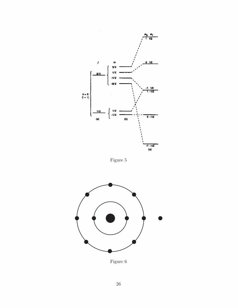
Figure 5

Figure 6

26

0

S

Ag source

Figure 7

27