historical var for bonds - a new approach

Historical VaR for bonds - a new approach

.................................................................................................................

.................................................................................................................

João Beleza SousaM2A/ADEETC, ISEL - Inst. Politecnico de Lisboa

Email: [email protected]

Manuel L. EsquívelCMA/DM FCT - Universidade Nova de Lisboa


Raquel M. GasparCEMAPRE,

ISEG, Universidade de LisboaEmail: [email protected]

Pedro. C. RealCMA/DM FCT - Universidade Nova de Lisboa


.................................................................................................................

Portuguese Finance Network 2014 - 1951 -

Bonds historical returns cannot be used directly to compute VaRbecause the maturities of returns implied by the historical prices donot have the relevant maturities to compute VaR. Given the so-calledpull-to-par in bonds, with return volatilities necessarily decreasingwith diminishing time-to-maturity,direct use of historical returns wouldlead to overestimation of the true VaR.Market practice deals with the problem of computing VaR for port-folios of bonds or mixed portfolios with cumbersome methods of cashflow mappings.In this paper we propose a new approach. We develop a techniqueto adjust bonds historical prices and extract from them an adjustedhistory of returns, that can be used directly to compute historical VaRfor bonds or bond portfolios.We illustrate the method using one concrete traded market zero-coupon bond, but the simplicity of the method makes this enoughto the reader to understand how it would work with coupon bonds,portfolios of bonds or mixed portfolios.

AbstrAct

- 1952 -Portuguese Finance Network 2014

1 Introduction

Despite all criticisms (see for instance [5]), historical simulation is still by farthe most popular VaR method for most securities, as argued in [4].

It is well known that VaR computation, by historical simulation, of bondportfolios differs in important ways from VaR computation of stock portfolios[2]. Essentially, this is because the market historical prices of bonds implyreturns with a variety maturities, none of them being the relevant maturityfor the purpose of VaR computations.

Consider, for instance, daily returns on a bond that has lived 5 years buthas still 2 years to maturity. The past daily returns have maturities from7 to 2 years: we have a different maturity for each daily return we observe.However the returns we are interested in simulating are the one associatedwith the next day(s), whose maturity we have no history about.

This moves away the possibility of using market bonds historical returns,directly in VaR computations.

The usual strategy to deal with this problem is via collecting historicalinformation on the entire term structure of interest rates (bootstrapping,interpolating, choosing a model, etc.) and then observe the evolution in timeof the exact cash-flows maturities, at the time we want to compute VaR. Thenone would still need to deal with aspects such as how to combine the VaRof the various, cash-flows (bucketing methods, etc). All this, to considerinterest rate risk alone. To include credit risk, correlation risk, etc manymore assumptions would have to be included using lots of different historicalinformation sources. There are books that dedicate many chapters to thismatter, and the authors themselves admit the methods are quite complex.For an overview of existing methods see [1].

This type of cash flow mapping methods by being subjective, and usinglots of information sources , ruin the objectivity and the simplicity underlyingthe ides of the VaR historical simulation. In the end of day, computationsare based upon estimations made using informations from other bonds andnot historical prices of the bonds that actually belong to the portfolio wewant to compute the VaR for.

Here we take a different approach and show the price history of the bondswe are interested in can indirectly be used to do all the necessary compu-tations. The method relies on one crucial assumption: mainly, that theyield-to-maturity (YTM) of a particular bond is a “good enough” measureof return that already takes into account “all” relevant risks (interest rate,

2


credit, liquidity, etc) for that bond. To us this seems easier to accept thanaccepting all assumptions, models, transition rating matrices, etc. needed toimplement the market practice method are correct.

Given historical prices (and thus YTM) on any bond, the proposed methodrelies on adjusting for the “pull-to-par effect” and obtaining an history ofpulled prices, based upon the historical YTM, but with the maturity rele-vant for the VaR computations.

Finally, when used for portfolios, the developed method strongly preservesthe market implicit correlations between the instruments in the portfolio.

The remaining of the paper is organized as follows. In Section 2 wepresent how to adjust bond return series for the purpose of VaR computa-tions. Section 3 illustrates the proposed method using real market quotes fora particular zero coupon bond. In Section 4.1 we show how to extend themethod to coupon bonds an portfolios of bonds and discuss other usages ofthe pulling technique. Finally, Section 5 concludes the paper summarizingthe main contributions to the literature. .

2 The Method

Consider the classical VaR computation at day nV aR, with time horizon Ndays, and confidence level α percent. For the sake of the argument and tointroduce notation, suppose we would be interested in computing the VaRof a bond in the same way we do it for stocks.

Following the classical approach 1, theN–days historically observed passedreturns should be used to compute VaR at date nV aR +N .

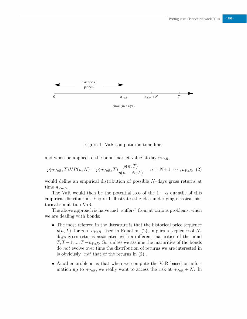
For simplicity, we consider a particular ZCB with maturity T > nV aR+Nand principal P . See the time line in Figure 1 for a graphical representationof these instants.

Let us denote by p(n, T ), the historical price of the ZCB at day n, forN < n ≤ nV aR < T , and by HR(n,N) the N–days historical return at dayn, defined as in [3].

Then the HR(n,N), possibly overlapping, historical gross returns aregiven by:

HR(n,N) =p(n, T )

p(n−N, T ), n = N + 1, · · · , nV aR, (1)

1VaR historical simulation method is referred by some authors as non-parametric VaR.

3


0 n VaR n VaR + N T

h istorical

p rices

tim e Hin d aysL

Figure 1: VaR computation time line.

and when be applied to the bond market value at day nV aR,

p(nV aR, T )HR(n,N) = p(nV aR, T )p(n, T )

p(n−N, T ), n = N+1, · · · , nV aR, (2)

would define an empirical distribution of possible N–days gross returns attime nV aR.

The VaR would then be the potential loss of the 1 − α quantile of thisempirical distribution. Figure 1 illustrates the idea underlying classical his-torical simulation VaR.

The above approach is naive and “suffers” from at various problems, whenwe are dealing with bonds:

• The most referred in the literature is that the historical price sequencep(n, T ), for n < nV aR, used in Equation (2), implies a sequence of N -days gross returns associated with a different maturities of the bondT, T −1, ..., T −nV aR. So, unless we assume the maturities of the bondsdo not evolve over time the distribution of returns we are interested inis obviously not that of the returns in (2) .

• Another problem, is that when we compute the VaR based on infor-mation up to nV aR, we really want to access the risk at nV aR + N . In

4


the case of bonds this is yet another maturity and, actually, the one wereally want to access the risk at.

• Besides the above mentioned shortcomings, the classical method alsosuffers from all the problems associated the historical VaR itself, inparticular, front the fact it uses the distribution of past returns toaccess future risk.

What one would like to know it would be the price p∗(n, T − nV aR) andp∗(n, T − nV aR − N), for all n with n < nV aR < nV aR + N . That is, wewould like have acess to historical prices on our ZCB with fixed maturitiesT − nV aR and T − nV aR −N . This information does not exist in the marketand needs to somehow to be estimated.

2.1 Existing Methods

Market practice focus on trying to get p∗(n, T−nV aR) and p∗(n, T−nV aR−N),estimating the daily evolution of the entire term structure of interest rates.This requires quite an effort and relies on a variety of bonds different fromthe one we are interested in (many of them possibly not even in our portfo-lio), interpolation methods, bootstrapping, adjusting for credit, liquidity andother risk, and strong model assumptions.

Theoretically, the methods allows us to obtain ZCB artificial prices p∗(t, T )for all possible t and T . It would not be surprising if, after so many oper-ations, the historical artificial prices of our concrete ZCB would differ fromthe true historical prices. If it is doubtful the method would work for ourparticular ZCB, it becomes even more questionable for big cash-flow matricescoming coupon paying bonds or bond’ portfolios. In that case one would alsoneed cash-flow mapping and bucketing methods.

2.2 Our approach

In this paper we propose a very different approach. Instead of focusing onthe history of the entire yield curve, whose exact meaning is questionable.After all each bond has its own YTM, and there is no such thing as a yieldcurve for a particular bonds.2

2For a particular bond there is only one YTM, for one (different) maturity each day.

5


Our proposal is to consider each bond individually doing the necessarymaturity adjustments to obtain the necessary returns. One would, then,compute the historical VaR for each bond, in a similar way one does forstocks. In our view this has the advantages of being simple, in line with thespirit of historical simulation VaR, and of using information actually availablein the market and related to the particular bond(s) in our portfolio. The ideais intuitively quite simple – we adjust past prices for the “pull-to-par” effect!

For all n < m we can define the pulled price f(m,n, T ) as the price pulledto time m, considering the YTM observed at time n, of our ZCB T–bond.

Based upon historical prices p(n, T ), we can define the implied daily com-pounded yield 3 r(n, T − n),

r(n, T − n) =

(P

p(n, T )

) 1T−n

− 1. (3)

We now define f(m,n, T ), the bond price pulled to time m and fixed bythe price p(n, T ) (at time n) for n < m < T , as :

f(m,n, T ) =P

(1 + r(n, T − n))T−m=

P(P

p(n,T )

)T−mT−n

. (4)

The relevant maturities for computing an N–day VaR at time nV aR areT−nV aR and T−(nV aR+N). Thus, will be interested in using past yields fromtime n, n < nV aR, to obtain prices pulled to the times nV aR and nV aR +N .

We can now define the nV aR time to maturity adjusted4 N–days historicalgross return at day n, denoted by AHR(n,N, nV ar), as the quotient betweenf(nV aR +N, n, T ) and f(nV aR, n−N, T ):

AHR(n,N, nV ar) =f(nV aR +N, n, T )

f(nV aR, n−N, T ), n = N + 1, · · · , nV aR. (5)

Substituting Equation (4) in Equation (5), we can rewrite the adjustedhistorical gross returns and obtain them directly from historical (market

3Daily compounded yields are used because typical VaR time horizons are specifiedin days. Alternative compounding could be used, but it does make sense to match thecompounding with the VaR horizon.

4Note adjusted returns are computed using pulled prices f(m,n, T ) and not historicalprices p(n, T ).

6


observed) prices:

AHR(n,N, nV ar) =

(P

p(n−N,T )

) T−nV aRT−(n−N)

(P

p(n,T )

)T−(nV aR+N)

T−n

, n = N + 1, · · · , nV aR. (6)

Note that the AHR(n,N, nV ar) value if fixed by historical market pricesp(n, T ) and p(n − N, T ), thus also capturing the pull-to-par effect and themarket changes in between n − N and n, while being adjusted to the VaRcomputation relevant maturities, namely, T − nV aR and T − (nV aR +N).

Our proposal is to replace the original historical returns of Equation (1)by those of Equation (6). Using these adjusted historical returns directly inthe VaR computation, the VaR is the potential loss of the 1 − α quantile ofthe following time to maturity adjusted empirical distribution:

p(nV aR, T )AHR(n,N, nV ar) = p(nV aR, T )f(nV aR +N, n, T )

f(nV aR, n−N, T )(7)

for n = N + 1, · · · , nV aR.

3 Illustration

In this section we illustrate the method using market data from a particu-lar zero coupon corporate bond, B. The prices were obtained from a quoteservice that delivers market prices aggregated from different dealers respon-sible for trading (market makers) this particular bond. Our bond B has aprincipal of P = 1000 and matures at day T = 731. We are standing at dayn = 372 (today) and will be interested in computing the 10–day VaR of thisparticular bond (N = 10). Figure 2 shows, in percentage, the real markethistorical prices. The prices in Figure 2 imply the evolution of yields in Fig-ure 3. Recall from Figure 3 that each day the YTM corresponds to a differenttime to maturity, marked in the graph top axis. Figure 3 clearly shows theusual trend observed in the market, in which smaller time to maturities aretraded with smaller implied returns.

3.1 Adjusting one return

For illustration purposes, consider we want to compute one single adjustedreturn for a VaR computation with N= 10 at time nV aR = 372. In particular

7


0 50 100 150 200 250 300 350

88

90

92

94

96

98

Day

Pri

ceH%L

Figure 2: Real historical prices of a zero coupon bond with principal P =1000 and maturing at day T = 731, as a percentage of the principal.

0 50 100 150 200 250 300 350

0

1

2

3

4

5

6

731 681 631 581 531 481 431 381

Day

Yie

ldH%L

Days to Matu rity

Yie

ldH%L

Figure 3: Daily compounded yields, implied by the historical prices of Figure2, as a function of both time and time to maturity.

8


0 50 100 150 200 250 300 350

88

90

92

94

96

98

Day

Pri

ceH%L

Historical p rices

Day 190 retu rn p rices

Fu tu re p rices at d ays 372 an d 382

Figure 4: The prices that determine the N = 10 days historical return attime n = 190, the corresponding future prices at times nV aR = 372 andnV aR + N = 372 + 10 = 382, along with the historical prices sequence. Thearrows represent future values.

we want to adjusted the historical return observed on n = 190, i.e we want tocompute is AHR(190, 10, 372). We observe the historical prices p(180, 731)and p(190, 731), associated with maturities 731−180 = 551 and 731−190 =541, respectively. But we would like to have the pulled prices for the VaRrelevant maturities, i.e., for the maturities T − nV aR = 731 − 372 = 359 andT − nV aR +N = 731 − 372 + 10 = 349.

Table 1 shows the market observed historical return at day n = 190, aswell as the corresponding adjusted return for VaR computed at day nV aR =372. The annualized daily yields to maturity and future prices used to com-pute the adjusted return are also detailed.

As it can be observed from Table 1 the adjusted return is closer to onethan the historical return. This is in accordance with the trend observed inFigure 3 and the annualized YTM computed in Table 1 . The prices thatdetermine this historical return are highlighted in Figure 4 with the blackcircles. While the pulled ones that determine adjusted historical returns arerepresented with black squares.

9


Historical gross return HR

p(190 − 10, 731) p(190, 731) HR(190, 10) = p(190,731)p(180,731)

94.25 95.03 1.00828

(a)

Annualized daily YTM (%)r(180, 551) r(190, 541)

4.001 3.499

(b)

Adjusted gross return AHR

f(372, 190 − 10, 731) f(372 + 10, 190, 731) AHR(190, 10, 372) = f(382,190,731)f(372,180,731)

96.215 96.765 1.00571

(c)

Table 1: (a) N = 10 days market observed historical return at day n = 190.(b) Days n = 180 and n = 190 annualized daily yields to maturity. (c)Adjusted N = 10 days return at day n = 190, for VaR computed at daynV aR = 372.

10


Time horizon Confidence level VaR Quantile CorrelationN = 10 α = 99% -9.576 -9.935 0.984

Table 2: Time horizon N = 10, confidence level α = 99%, bond B VaR, com-puted at day nV aR = 372 by historical simulation using adjusted historicalreturns.

3.2 Computing VaR

Consider the VaR, with a time horizon of N = 10 days and confidence levelα = 99%, computed by historical simulation, at day nV aR = 372, of theportfolio containing the bond B.

We want to obtain the entire empirical distribution of all possible 10days returns. The maturities we are interested in are 731 − 372 = 359 and731 − 382 = 349 days to maturity. In order to obtain this distributionwe adjust each of the historical returns with Equation (6). The VaR is,then, computed using the empirical distribution of the adjusted returns ofEquation (6). In order to obtain this distribution the adjustment of thesingle return detailed in the previous section is repeated for all availablehistorical returns. Figure 5 shows the real, market observed historical prices,and also, the corresponding pulled prices, f(m,n, T ) of Equation (4), to daysm = nV aR = 372 and m = nV aR + N = 372 + 10 = 382. The pulled pricesare plotted as a function of the day n of the historical price p(n, T ) whichfixes the yield value f(m,n, T ). The prices highlighted in Figure 4 with theblack circles and squares are highlighted again in Figure 5, but now plottedas a function of n.

Figure 6 shows the sequence of the bond’s historical returns along with thesequence of the corresponding adjusted returns computed from the ficticiousprices of Figure 5. Figure 7 shows the respective histograms.

Finally, Table 2 shows the VaR value computed from the empirical dis-tribution of the overlapping adjusted returns of Equation (7), along with thepossible loss corresponding to 1 − α quantile of the overlapping historicalreturns empirical distribution of Equation (2), for comparison purposes. Italso shows the correlation coefficient between the original and the adjustedreturns.

As it can be observed from Figure 6, the adjusted returns are closer toone than the historical ones. This can be observed as well in Figure 7 wherethe adjusted returns histogram is more concentrated towards one than the

11


0 50 100 150 200 250 300 350

88

90

92

94

96

98

Day

Pri

ceH%L

Historical p rices

Fu tu re p rices at tim e 372

Fu tu re p rices at tim e 382


Fu tu re p rices at d ays 372 an d 382

Figure 5: Historical prices, and the corresponding pulled prices at timesm = nV aR = 372 and m = nV aR + N = 372 + 10 = 382. The pulled pricesare plotted as a function of the time n, of the historical price p(n), that fixedthe future price.

0 50 100 150 200 250

0.99

1.00

1.01

1.02

1.03

1.04

Day

Re

turn

Historical re tu rn s

Ad ju sted retu rn s

Figure 6: Historical returns and the corresponding adjusted returns fornV aR = 372.

12


Historical returns Adjusted returns

0.96 0.98 1.00 1.02 1.04

5

10

15

20

Figure 7: Historical returns and the corresponding adjusted for nV aR = 372returns, histograms.

historical returns histogram. This results in a VaR value smaller than thecorresponding loss of the 1−α/100 quantile of the possible historical returns.Again, this result conforms with Figure 3 which shows a clear decreasingtrend in interest rate as time to maturity decreases.

4 Other usages and Extensions

In this section we show how the “pulling of prices” proposed in the previoussection can be also useful for other purposes – like inferring from the historyof other bonds, history on just issued bonds – and we discuss the extensionVaR method developed to coupon bonds and bond portfolios.

4.1 Adjusting for past values

Suppose that the bond B has already expired and its issuer issues a newbond, B1, similar to bond B. I.e., with the same type, principal, maturity,number of coupons, coupon rate (if applicable), etc.

Consider a portfolio that contains the bond B1. The portfolio VaR with

13


Time horizon Confidence level VaR Quantile CorrelationN = 10 α = 99% -20.291 -9.935 0.985

Table 3: Time horizon N = 10, confidence level α = 99%, bond B VaR,computed at day nV aR = 1 by historical simulation using adjusted historicalreturns.

time horizon N days is to be computed by historical simulation at day 1.The only historical prices available from bond’s B1 issuer are those of bondB.

The adjustment method proposed in this paper can still be applied topull the historical prices of bond B to past times, times before the historicalprices were observed, namely, for day 1. The process is the same as forfuture dates: for each historical price compute the daily yield to maturityimplied by the historical price; than compute the bond’s value at a previoustime valuing the bond’s cash flows following the time considered, with theimplied daily yield to maturity; finally use the previous times values to getthe adjusted returns of Equation (5), and compute the VaR.

Consider the portfolio containing the bond B1 and the VaR computedby historical simulation at day n = 1 with the historical prices of bond B,showed in Figure 2.

Following section 4.1 the past values of Equation (4), f(m,n) with m =1 ≤ n are used to compute the adjusted historical returns of Equation (6)and the vaR is computed from the resulting empirical distribution. In thissection we illustrate this process by repeating the figures and the table of theprevious section, but now, for nV aR = 1.

It can be observed from Figure 11 that the adjusted returns are nowless concentrated towards one than the historical returns. This results in aVaR value, showed in Table 3, which is now greater than the correspondingloss of the 1 − α/100 quantile of the possible historical returns. Again,this observation in accordance with Figure 3 and the fact that the time tomaturity at time VaR is computed, nV aR = 1, is greater that the times tomaturity at following times, namely, when the historical prices were observed.

4.2 Coupon bonds

The extension to coupon bonds is straight forward. In order to compute thepulled price of a coupon bond at time m, based on the market price of the

14


0 50 100 150 200 250 300 350

88

90

92

94

96

98

Day

Pri

ceH%L

Historical p rices


Past p rices at d ays 1 an d 11

Figure 8: The prices that determine the N = 10 days historical return at timen = 190, the corresponding past prices at times nV aR = 1 and nV aR + N =1 + 10 = 11, along with the historical prices sequence. The arrows representpast values.

15


0 50 100 150 200 250 300 350

88

90

92

94

96

98

Day

Pri

ceH%L

Historical p rices

Past p rices at tim e 1

Past p rices at tim e 11


Past p rices at d ays 1 an d 11

Figure 9: Historical prices, and the corresponding past prices at times m =nV aR = 1 and m = nV aR + N = 1 + 10 = 11. The past prices are plottedas a function of the time n, of the historical price p(n), that fixed the futureprice.

0 50 100 150 200 250

0.98

0.99

1.00

1.01

1.02

1.03

1.04

Day

Re

turn

Historical re tu rn s

Ad ju sted retu rn s

Figure 10: Historical returns and the corresponding adjusted returns fornV aR = 1.

16


Historical returns Adjusted returns

0.96 0.98 1.00 1.02 1.04

2

4

6

8

10

12

14

Figure 11: Historical returns and the corresponding adjusted for nV aR = 1returns, histograms.

bond at time n < m, two differences from the zero coupon bond case arise:

• the yield to maturity at time n is computed using the bond’s dirty priceand accounting for all future cash flows after time n;

• the value of the bond at time m accounts for all future cash flows aftertime m.

Then, the adjusted returns are defined by Equation (6) as in the case of azero coupon bond and the VaR is computing as the loss corresponding to thequantile of the empirical distribution of Equation (7).

Using the proposed approach dealing with portfolios of bonds or mixedportfolios should be not harder than dealing with stock portfolios, providedwe alwasys consider the adjusted returns history and not the actual returns.

5 Conclusions

Bond historical returns can not be used directly to compute VaR by historicalsimulation because the maturities of the yields implied by the historical pricesare not the relevant maturities at time VaR is to be computed.

17


In this paper we adjust bonds historical returns so that the adjustedreturns can be used directly to compute VaR by historical simulation. Theadjustment is based on pulled prices, extracted from historical prices, andpulled to the maturities relevant for the VaR computation.

The proposed method has the following features:

• The time to maturity adjusted bond returns are used directly in theVaR historical simulation computation.

• VaR of portfolios with bonds can be computed by historical simulationkeeping the simplicity of the historical simulation method.

• The portfolio specific VaR is obtained.

• The VaR values obtained are consistent with the usual market trendof smaller times to maturity being traded with smaller interest rates,therefore carrying smaller risk and having a smaller VaR.

• The only source of information used is the market, through the bondshistorical prices.

• The correlation between each bond return and the returns of the otherinstruments in the portfolio is strongly preserved.

• The VaR for the desired time horizon is computed directly with no VaRtime scaling approximations.

We left for future work, the research of the mathematical properties of thedeveloped method, and backtesting the method with benchmark portfolios.

References

[1] C. Alexander. Market Risk Analysis, Value at Risk Models. John Wiley& Sons, 2009.

[2] Gangadhar Darbha. Value-at-risk for fixed income portfolios a compar-ison of alternative models. Technical report, National Stock Exchange,Mumbai, 2001.

[3] John C. Hull. Options, Futures, and Other Derivatives. Prentice Hall, 7edition, 2008.

18


[4] Christophe Perignon and Daniel R. Smith. The level and quality of value-at-risk disclosure by commercial banks. Journal of Banking & Finance,34(2):362 – 377, 2010.

[5] Matthew Pritsker. The hidden dangers of historical simulation. Journalof Banking & Finance, 30(2):561–582, February 2006.

19


historical var for bonds - a new approach

Documents