Historical Perspectives on Financial Development and Economic Growth

by

Peter L. Rousseau’~

Final revision: January 2003

a - Associate Professor of Economics, Vanderbilt University, Box 1819 Station B, Nashville, TN

37235, USA and Research Associate, National Bureau ofEconomic Research. E-mail to

peter.!. rousseau(~vanderbiit. edu. The author thanks Hendrik Houthakker, Larry Neal, Richard

Sylla, Paul Wachtel, Eugene White, and conference participants for useful comments and

suggestions.

The link between financial development and economic growth is not a recent discovery. And

though Bagheot (1873), Schumpeter (1911), and Gurley and Shaw (1955) motivated thisrelationship

decades, and indeed, over a century ago, it remained for economic historians such as Davis (1965),

Cameron (1967), and Sylla (1969), among others, to give empirical content to the idea. These

scholars primarily used the historical experiences of England and the United States to illustrate the

role ofthe financial system in the paving the way to market leadership. Since then, macro and

development economists have studied the link more formally with theoretical models in which

countries achieve rapid growth through well-developed financial systems that reduce credit market

frictions (e.g., Greenwood and Jovanovic, 1990, Greenwood and Smith, 1997, andRousseau, 1998),

and with cross-country andtime series statistical studies that uncover significant effects of financial

sector size on macroeconomic outcomes (e.g., King and Levine, 1993, and Rousseau and Wachtel,

1998).’

Interestingly, economic historians and macro economists studying finance and growth seem

for the most part content to continue pursuing their closely-related agendas independently. Perhaps

this is because macro economists usually ask whether financial factors do indeed matter for growth,

while most economic historians see the answer to this question as more obvious, and ask instead how

and how much they matter. The economic historian’s prior is understandable — older single-country

studies have made strong cases for finance-led growth with the sporadic data observations that are

usually available. For the macro economist, however, the lack of an explicit role for financial factors

in the baseline neoclassical growth model combines with a recognition of the statistical and

conceptual problems of establishing causation in cross-country and time series regressions to yield a

‘The empirical literature on the so-called “finance-growth nexus” has expanded rapidly in recent

years, making an exhaustive list of references impractical to provide here. Levine (1997) offers a

useful survey.

more cautious perspective. This article attempts to narrow the gap between these views by

illustrating with standard macro-econometric techniques that the historical time series that are

available for Amsterdam (1640-1794), England (1720-1850), the United States (1790-1850), and

Meiji Japan (1880-1913) are consistent with the “finance-led” growth hypothesis.

The approach is decidedly macro economic. This is because I believe that the empirical

growth literature has under-emphasized a keymechanism through which finance matters in the early

stages of economic development— resource mobilization. This is not to say that banks and financial

markets do not also promote growth by directing resources to productive uses, but that their ability to

overcome project indivisibilities and to encourage investors to accept longer time horizons for

payoffs widens the first bottleneck through which a young economy must pass. This turns out to be

important for the four countries that I consider in this study, and especially for the Dutch Republic,

England, andthe United States, whose financial sectors emerged during their “pre-industrial”

epochs. Is it no coincidence that England, with the keycomponents of a financial system in place by

1750, was poised to tackle industrialization next? The main findings suggest that banks and financial

markets did indeed promote investment and commercial activities by generating information,

pooling funds, facilitating payments, and providing working capital for the largest companies that

traded on the world’s earliest “stock exchanges,” at least in the modern sense of the term.

The article proceeds on a case-by-case basis, but will, to the degree that it is practical, offer a

consistent empirical framework throughout. At the end, I summarize some ofmy recent findings

with Richard Sylla for a larger group of countries afier 1850. It seems only appropriate to begin the

analysis with the city of Amsterdam, the site where the actionbegins.

2

AMSTERDAM

The World’s First Financial Revolution?

Amsterdam rose to prominence as a commercial city in the late 16th century. Its strategic

position in the North Sea for intra-European and Baltic trade made it a logical heir to the inheritance

of Antwerp, which had been the center of European commerce over the preceding century (van der

Wee, 1963). As the largest city in the newly-formed United Provinces, Amsterdam’s reputation for

ethnic tolerance also drew immigrants and their capital from the rest ofEurope and the Eastern

Mediterranean. These factors combined by the early 17th century to produce a bustling commercial

community. As the potential for speculation and profit in trading with the East Indies became clear,

Amsterdam merchants began pooling resources to equip individual voyages, with the profits

distributed upon sale of the incoming cargoes. These arrangements were formalized in 1602 with the

chartering ofthe United East India Company (or VOC, short for Vereenigde Oostindische

Compagnie). The charter called for a combine from six cities, or chambers, of which Amsterdam

was by far the largest and most important. The VOC was capitalized with 2,167 shares at a par value

of 3,000 forms each, and the owners could liquidate their stakes through the Company once every

ten years (Glamann, 1958, pp. 7-8). But when the Directors repudiated this provision at the end of

the first decade, those wishing to liquidate needed a secondary market. It was in this climate that

shares and futures began to trade on the Amsterdam bourse — the world’s first modern securities

market ifwe are to believe the engaging anecdotes of Joseph de Ia Vega (1688).

The VOC was Amsterdam’s largest trading company and held a monopoly by statute and in

practice on Asiatic trade east of the Cape of Good Hope, but other forms of commerce, especially

intra-European, also flourished in Amsterdam throughout the 17th century. It was decided early on

that the city would need a clearinghouse for exchange, and the Bank of Amsterdam got started in

3

1609 to perform this function. And though the innovations of a clearing bank and exchange bills did

not originate in Amsterdam, having existed previously in Venice and Antwerp, never before had

either form been used so successfully.

The Bank of Amsterdam (BA) was not a bank of issue, but instead accepted bullion and coin

from merchants and held them for safekeeping, issuing receipts for “drawing accounts” that could be

used for exchanging wealth as needed in the course oftrade. The Bank also made large loans to the

VOC and to the government over the next two centuries (to the latter for waging wars). According to

de la Vega (pp. 23-24), however, the Bank did not only support commodity trades, but was also used

to effect payments. For example, stocks traded on the bourse were often said to be “payable at the

Bank,”and“time accounts” organized by the Bank were used as quasi-official records of futures

agreements — records in which sellers could attest that they actually held the security that they had

agreed to deliver and in which borrowers could record their intention to borrow whenthe time came

to settle or purchase.2 It was in this manner that the Bank and its drawing accounts became a key

component ofthe stock exchange.

Data and Methodology

To explore quantitatively the relationship between finance and growth in pre-Industrial

Amsterdam, some measures of commercial investment and of financial size and efficiency are

needed. And though there are few continuous time series from the period, there are enough to

conduct a preliminary statistical investigation. Van Dillen (1934, pp. 117-123), for example,

published annual figures for the Bank of Amsterdam’s activities from 1610 through 1820, including

the balances in its “drawing” accounts and loans to the VOC. To the extentthat the BA supported the

2 See also Hermann Kellenbenz’s (1957, p. 18) introduction to the English translation of de la

Vega.

4

stock market and commerce in Amsterdam during this period, the size ofits drawing accounts may

be a reasonable measure of the city’s financial development. Further, Neal (1990) has improved

upon van Dillen’s (1931) share price series for the VOC from 1723 through 1794.~I will use these

data to explore the efficiency of the Amsterdam market and the importance of any financing

constraints that the VOC might have faced. Measures of aggregate investment in the city are not

generally available, but the VOC archives do include the number ofvoyages that the Company sent

to the East Indies in each year from 1641 to 1794, the amounts of gold, silver, and coins that left with

these voyages, andthe market values of their incoming cargoes.4 If investment and trading activity in

the VOC reflect commercial activity in Amsterdam more broadly, testing for statistical links between

drawing balances at the BA andVOC investment might shed some light on how finance affected real

activity at the time. Figure 1 shows the evolution of the form-denominated real quantities as three-

~To build the annual series, I use the final price observation in each year for VOC shares from

Neal’s reading of the Amsterdam Courant. These observations are usually from the last week in

December. I use the final price observations from van Dillen (1931) foryears that are unavailable in

Neal’s data. The VOC prices and other stock market data from Neal (1990) are available on the

world-wide web from the Inter-University Consortium for Political and Social Research (ICPSR) at

the address http://www.icpsr.umich.edu.

~The number of outgoing VOC voyages is from the Netherlands Historical DataArchive’s

(NHDA) Data Set D0100 titled “Dutch-Asiatic shipping, 1602-1795.” The data are similar but not

identical to those presented in Bruijn, Gaastra, and Schoffer (1987). Eastbound money shipments are

from NHDA Data Set F3503 titled “Total amounts of money, 1603-1795.” The market value of VOC

trade is from NHDA Data Set No. F3505 titled “Returning ships and products, 1641-1796.”

5

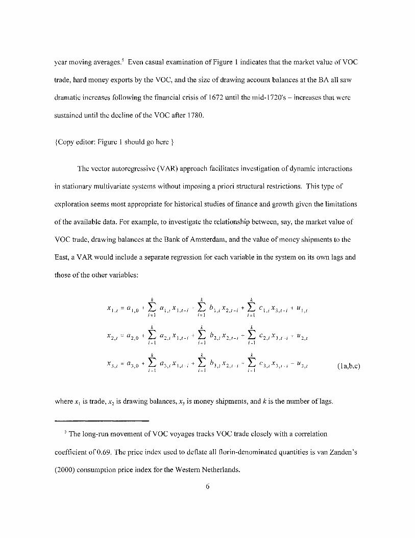
year moving averages.5 Even casual examination of Figure 1 indicates that the market value ofVOC

trade, hard money exports by the VOC, and the size of drawing account balances at the BA all saw

dramatic increases following the financial crisis of 1672 until the mid-1720’s — increases that were

sustained until the decline ofthe VOC after 1780.

{Copy editor: Figure 1 should go here }

The vector autoregressive (VAR) approach facilitates investigation of dynamic interactions

in stationary multivariate systems without imposing a priori structural restrictions. This type of

exploration seems most appropriate for historical studies of finance and growth given the limitations

of the available data. For example, to investigate the relationship between, say, the market value of

VOC trade, drawing balances at the Bank of Amsterdam, and the value of money shipments to the

East, a VAR would include a separate regression for each variable in the system on its own lags and

those ofthe other variables:

x1, = a10 + aiixiti + b,1x~1~+ c~x31~1+ u1,

x2, = a20 + a21x111 + b21x2~_1+ c~x31~+ u2~

x3, = a30 + a31 X11~~

+ ~ b3~x214 + k c31 X311

+ U31

(la,b,c)

where x, is trade, x2 is drawing balances, x3 is money shipments, and k is the number of lags.

The long-run movement of VOC voyages tracks VOC trade closely with a correlation

coefficient of 0.69. The price index used to deflate all form-denominated quantities is van Zanden’s

(2000) consumption price index for the Western Netherlands.

6

Stationarity of a VAR is important in interpreting tests for Granger non-causality, that is the

hypothesis that past values of a variable do not jointly improve one-step ahead forecasts of another.

Specifically, the null hypothesis implies the following joint restrictions on the coefficients in (1):

1j,i = ~ = = ‘J,k = 0 l=a,b,c; j=l,2,3. (2)

In general, the distributions of these tests are nonstandard when a VAR contains variables with unit

roots, and differencing is usually required to ensure stationarity. Sims, Stock, and Watson (1990)

show, however, that Granger tests conform to standard distributions in tn-variate VARs with unit

roots so long as a cointegrating relationship exists among the variables. I apply this result in the

eight tn-variate systems for Amsterdam because the null hypothesis of a unit root is not rejected with

standard tests for any of the variables and there appears to be comntegrating relationship in each

system.6 Running a VAR in levels is advantageous because it allowsjoint evaluation of short and

long-term effects ofmovements in one variable upon others in the system.

Granger-causality tests must be interpreted cautiously since rejection ofthe block exclusion

restrictions does not necessarily imply that there is “economic causality.” This is because the

validity of the test is predicated on the inclusion of the full information set in the VAR. Since this

condition is violated in any finite regression framework, especially when the data at hand are only

proxies for the desired theoretical constructs, the seemingly-strong results presented below are

suggestive ofthe nature of linkages between finance and investment in pre-Industrial Amsterdam but

cannot be taken as conclusive.

When an investigator can specify a reasonable causal ordering for the variables in a VAR

system (based on economic theory and perhaps the results of Granger tests), the nonlinear responses

of each variable to one-time shocks in the others can be traced through time. This facilitates an

6 See the Appendix for details and results of tests for unit roots and cointegration.

7

evaluation of the economic importance (i.e., size) ofthe estimated effects, and for this reason I

augment the results of Granger-causality tests with an examination of selected impulse responses.

Finance and VOC Investment

Table 1 presents estimates from four VARs that cover the period from 1641 to 1794. The

starting year is that in which all data become continuously available, and the end date was chosen to

capture the decline of the United Provinces but not the period ofpolitical upheaval that surrounded

the French invasion of 1795. Nested likelihood ratio tests select three lags.7 For each system, I report

the sum of the regression coefficients on the variable blocks listed in the column headings in

equations (la)-(lc) along with the significance level of the F-test for block exclusion. In the upper

left panel, for example, the results for equation (la) indicate that the log of real drawing balances at

the Bank ofAmsterdam Granger-cause the real market value ofVOC trade at the 1 percent level,

while real money exports Granger-cause trade at the 6 percent level. The coefficients on the lag

variables sum to a positive number for each ofthese blocks. Equation (ib) shows that neither trade

nor money shipments Granger-cause BA drawing balances, while equation (1 c) shows that BA

balances Granger-cause money shipments.

{Copy editor: Table 1 should go here }

The results are qualitatively similar in the upper-right panel ofTable 1, where the log of

outgoing VOC voyages replaces VOC trade as the measure of investment, though money shipments

are no longer statistically significant in equation (1 a). These findings suggest that increases in the

size ofthe BA’s drawing account balances did indeed have a positive effect on commercial activity.

~This method starts with a sufficiently large lag length and then tests successively that the

coefficients on the final lag are zero, stopping when the restrictions are rejected.

8

Further, larger balances increased the amount of hard money that was used in conducting VOC

business. This seems reasonable, as more resources at the disposal of the Bank would make it easier

to meet demands for bullion prior to ship departures. There is no evidence of feedback from either

trade or investment to drawing account balances or money exports. Thus, the effects of the financial

variables appear to be unidirectional.

{Copy editor: Figure 2 should go here }

Figure 2 shows the impulse responses. The Granger-causality tests in Table 1 imply that

placing drawing account balances first, money exports second, and either investment or trade third

would move from the most statistically “exogenous” variable to the least. In panels (a) and (b), a 1

percent change in BA balances is related to an increase in VOC trade of about 0.45 percent after two

years and a sharp increase in VOC voyages of about 0.3 percent. Both effects decay slowly.

Evaluated at the sample means, the responses imply that increasing BA balances by 1.6 mu. forms

(10 percent) would increase VOC trade by 2.8 mu. forms and lead to 3.7 additional voyages over the

next five years. These increases would have been substantial given that drawing balances at the Bank

were used to support all types of commercial activity in the city, not just that of the VOC. Panel (c)

shows that a 1 percent change in the amount of gold, silver, and coin sent East by the VOC led to

return cargoes that were about 0.26 percent larger. Evaluated at the sample means, this implies that

for every form in precious metals sent out, incoming cargoes over the next five years were worth 3.7

forms more. The VOC seems to have deployed its metallic resources efficiently in the East Indies.

In panel (d), a one percent change in BA balances is associated with a 3.4 percent increase in VOC

money exports over a 5-year period.

In the lower panels of Table 1, I switch to a specification in real levels (i.e., without taking

9

logs) to allow the outstanding debt ofthe VOC at the Bank of Amsterdam, which contains zero

values in several years, to enter the systems in place ofmoney exports. I did this as an initial test of

whether the VOC faced financing constraints in its operations. Interestingly, VOC debt does not

Granger-cause VOC investment in either systems, though it does respondnegatively to increased

trade and shipping activity. This might mean that when the Company needed to get voyages

underway, the Bank did not stand in the way of providing working capital, andthat once equipped,

the VOC’s demand for debt fell off. This is not the type of behavior that one would expect from a

company that was having trouble raising cash in the local financial market.

Finance and the Q-Theory ofInvestment

The Q-theory of investment as first described by Brainard and Tobin (1968) predicts that a

firm’s investment rate will rise with its Q (the ratio ofmarket value to the replacement cost of

capital). Fazarri, Hubbard and Peterson’s (1988, FHP) study of financing behavior among U.S. firms

in the 1980’s, however, casts doubt on a single-factor Q-theory in favor of one in which access to the

capital market figures prominently. Indeed, FHP’s firm-level regressions show that cash flow

explains investment more effectively than a host of alternatives and that Q loses some of its

explanatory power when cash is included in the model. This is especiallytrue for firms with low

dividend payout ratios where in some specifications Q loses statistical significance altogether. This

effect probably occurs because firms with low payout ratios are often small firms that have limited

access to external capital, which makes financing constraints bind more sharply when borrowing

channels dry up. Since the VOC was a large company, one would not expect it to face financing

constraints in today’s relatively efficient U.S. capital market, but it certainly might face them in a

less developed market due to the effects ofthe business-cycle on the availability of loanable funds.

10

{Copy editor: Table 2 should go here }

The VARs reported in Table 2 examine whether such constraints were active between 1723

and 1794, which is the period when continuous annual prices of VOC shares become available (see

fu. 3). Like their counterparts in Table 1, these systems include either the market value of VOC trade

or the number of outgoing voyages as measures of investment, but now also include the VOC ‘5 Q at

the end of each year.8 By then adding either drawing account balances or VOC debt at the BA, I can

examine whether Q is indeed the only determinant of investment as the theory would suggest, or

whether, as in FHP, the other financing variables come in strongly and lower the estimated

coefficients on Q. The results in Table 2 are striking in that Q matters for explaining VOC

investment (equation 1a) in all four VARs, while neither drawing balances nor VOC debt are

significant determinants. Taken alongside Table 1, this suggests that VOC investment did not only

grow with the capital market, but that temporary fluctuations in credit conditions within the Bank of

Amsterdam did not alter capital budgeting decisions being made by the Company Directors. Rather,

the Amsterdam capital market was liquid enough for the VOC to secure the funds needed for

investment based on its shadow price and did not rely on the official bank of exchange. This seems

to reflect financial development in a most fundamental sense.

ENGLAND

Finance, Trade, and the Industrial Revolution

England’s “financial revolution” can be traced to Dutch innovation that accompanied

William III as he crossed the North Sea to accept the British throne in 1688, but the event really

8 The VOC did not change its share capital over the 71-year period that I consider so that the Q of

VOC equity is the ratio ofprice to par value of the shares.

11

involved two phases — the first being pre-Industrial and the second Industrial. It is fortunate that the

financial institutions that arose to facilitate both internal and external trade and to stabilize the

monetary system in the half-century after the Glorious Revolution left the nation poised to overcome

the political and social obstacles of financing an Industrial Revolution.

British finance got a strong start with the founding of the Bank of England (BE) in 1694.

Over its first fifty years, the BE would become, to quote R. D. Richards (1934, p. 272), “a credit

institution, an organ of State Finance, a discount and issuing house, a bullion warehouse, and a safe

repository.” Shortly after its founding, the government hadthe nation’s metallic currency re-coined

and the Bank engaged in various note-issuing experiments, both of whichpromoted monetization of

the economy and brought some order to a disheveled monetary system. And while the Bank’s

integral relationship with the State has received the most attention among its scholars, the Bank’s

support of London’s merchant and trading communities through its clearing and discounting

facilities was too large to be overlooked (see Clapham, 1941). Indeed, it is the monetization and the

private business roles of the Bank that I will focus upon in this section.

Before 1750, the Bank of England co-existed only with a group ofprivate bankers in London

who dealt primarily in deposits and bills of exchange. This gave rise to an active money market to

finance trade and working capital for the fledgling manufacturing sector, and the BE played a key

role in its smooth operation. A stock exchange emerged by the 1690’s to facilitate transactions in

public debt securities and shares of the large trading companies, including the British East and West

India Companies, the South Sea Company, and the Royal African Company. In short, England

quickly achieved what Richard Sylla and I have listed as four of the five elements of a “good”

financial system: (1) sound public finance, (ii) stable money, (iii) a central bank, and (iv) well-

functioning securities markets (Rousseau and Sylla, 2001, pp. 2-3).

12

With a reasonably “good” system in place by 1750, it remained for the financial sector to

develop the final feature: (v) a variety ofbanks. Indeed, country banks did not spring up until the

second half of the 18th century, but made up for lost time by multiplying rapidly, issuing their own

notes to facilitate transactions outside ofLondon, and fostering correspondent relationships with

London’s private bankers.9 Savings banks started up after 1817 to provide a vehicle for the surpluses

of less-wealthy individuals, but were never large enough to be a very important part ofthe financial

landscape. Major legislation enacted in 1826 ended the BE’s long-standing monopoly in the joint-

stock banking business, and though institutions (perhaps surprisingly) did not form immediately in

response, by 1840 there were more than 600 joint-stock banks.

Amidst such important financial advances, England was also undergoing a commercial and

industrial revolution. Figure 3 shows that the real value ofinternational trade, defined as the sum of

imports, domestic exports, andre-exports, rose by 50 percent between 1720 and 1760, and another

50 percent between 1760 and l805.’°When viewed alongside earlier data for the English East India

Relatively little is known about the extent of country banking in 18th century England and its

contributionto the money supply beyond the information contained in Pressnell (1956). We do

know, however, that country banks were generally small and grew rapidly in number after 1750.

Cameron (1967, pp. 23-24), for example, reports that “about a dozen” existed in 1750, more than

100 in the early 1780’s, more than 300 by 1800, and 783 in 1810.

‘° The trade data are from Mitchell (1988), Table 10.1.A, pp. 448-449 for England and Wales

1720-1791, Table lO.l.B, p. 450 for Great Britain 1792-1804, and Table 10.2, pp. 451-452 for the

U.K. 1805-1850. I start with the earlier and more narrow trade figures for England and Wales and

then successively join the broader aggregates to form a single trade series. I form the price deflator

using Mitchell (1988) by joining the Schumpeter-Gilboy index for consumer goods for 1720-1819

13

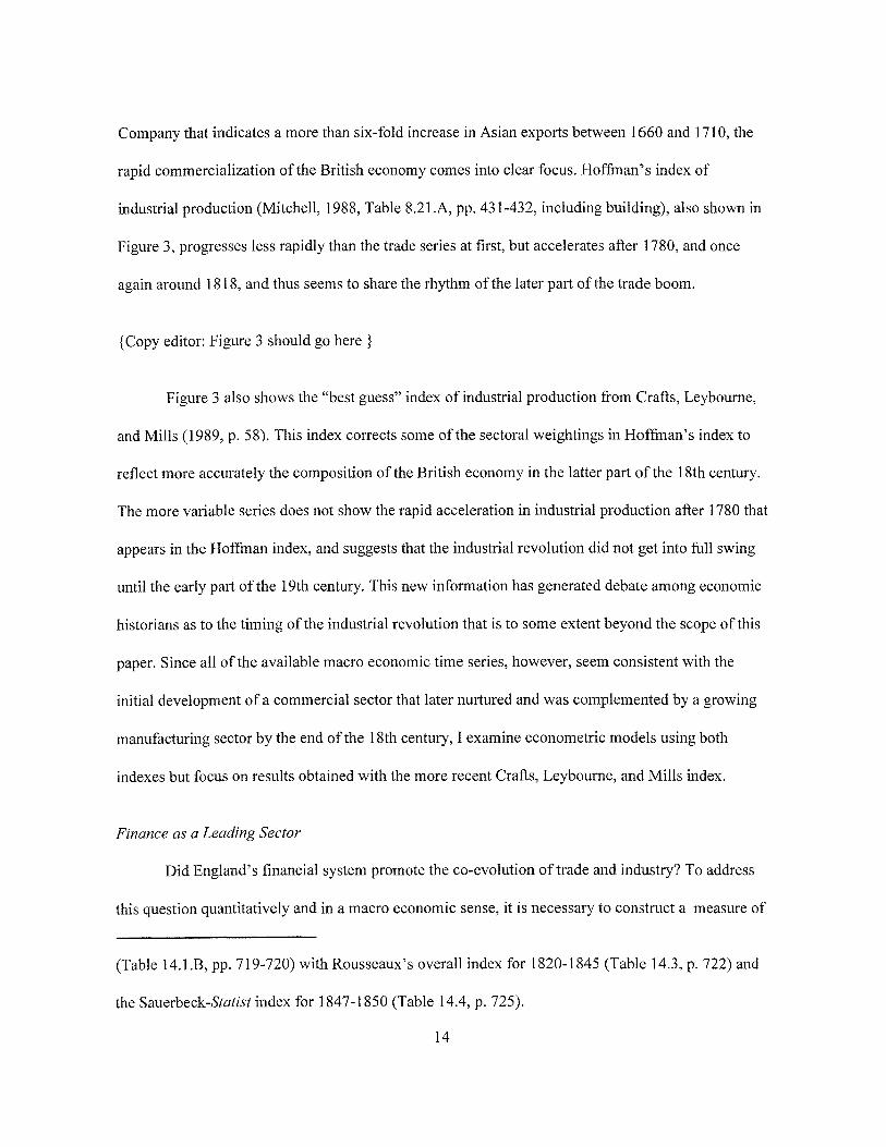
Company that indicates a more than six-fold increase in Asian exports between 1660 and 1710, the

rapid commercialization of the British economy comes into clear focus. Hoffiuian’s index of

industrial production (Mitchell, 1988, Table 8.21 .A, pp. 431-432, including building), also shown in

Figure 3, progresses less rapidly than the trade series at first, but accelerates after 1780, and once

again around 1818, and thus seems to share the rhythm of the later part of the trade boom.

{Copy editor: Figure 3 should go here }

Figure 3 also shows the “best guess” index of industrial production from Crafts, Leybourne,

and Mills (1989, p. 58). This index corrects some ofthe sectoral weightings in Hoffman’s index to

reflect more accurately the composition of the British economy in the latter part of the 18th century.

The more variable series does not show the rapid acceleration in industrial production after 1780 that

appears in the Hoffman index, and suggests that the industrial revolution did not get into full swing

until the early part of the 19th century. This new information has generated debate among economic

historians as to the timing of the industrial revolution that is to some extent beyond the scope of this

paper. Since all of the available macro economic time series, however, seem consistent with the

initial development of a commercial sector that later nurtured and was complemented by a growing

manufacturing sector by the end ofthe 18th century, I examine econometric models usingboth

indexes but focus on results obtained with the more recent Crafts, Leybourne, and Mills index.

Finance as a Leading Sector

Did England’s financial system promote the co-evolution of trade and industry? To address

this question quantitatively and in a macro economic sense, it is necessary to construct a measure of

(Table 14.1.B, pp. 719-720) with Rousseaux’s overall index for 1820-1845 (Table 14.3, p. 722) and

the Sauerbeck-Statist index for 1847-1850 (Table 14.4, p. 725).

14

monetization. This is easier for the period before 1775 because London’s private bankers had

stopped issuing notes, which had always been a small part oftheir business, years earlier due to

competition from the BE (Cameron, 1967, p. 22). It is thus fair to say that coin and BE notes made

up the circulating medium used in London before 1750 and a large part of what circulated outside of

the city as well. This is useful because time series for the circulation and deposit liabilities ofthe BE

are available almost from its inception. The rise of deposit banking in the countryside after 1775 and

a lack of reliable information about net specie imports, however, doom any attempt to build a

continuous series for an M2 aggregate. Nevertheless, Figure 4 shows a strong long-term relationship

between the BE’s deposit and circulation liabilities and Cameron’s (1967, p. 42) sporadic estimates

of the broad money supply.” Further, Huffman and Lothian’s (1980) estimates of high-powered

money for the 1833-1850 period (not shown) track BE liabilities closely from 1840 to 1850, which is

the period when the issues of the joint-stock banks make the trend ofthe BE series first begin to

diverge from the pattern in Cameron’s estimates. These observations offer reason to believe that the

BE’s deposit and circulation liabilities are useful as a proxy for long-term fluctuations in narrowly-

defined money, andperhaps even as a more general measure of monetization.

{Copy editor: Figure 4 should go here }

~‘ The circulation and deposit liabilities ofthe Bank of England are from Mitchell (1988, Table

12.2.A, pp. 655-658). I reconstructed a series for the Bank’s private advances as the income from

discounting bills and notes and making private loans (Clapham, 1945, Vol. I, Appendix E, pp. 301-

302, andVol. II, Appendix C, p. 433) divided by the Bank rate over the previous year (Clapham,

1945, Vol. I, Appendix D, p. 299, discount rates for inland bills, and Vol. II, Appendix B, pp. 429.

This assumes that the BE’s loans were primarily short term, which is consistent with Clapham’s

reading ofthe loan records.

15

Part ofthe Bank’s business was in making advances to merchants with drawing accounts,

though not all those with accounts were entitled to discount (Clapham, 1941). The Bank also made

over ninety loans to the East India Company between 1709 and 1744, but these direct loans, though

exceeding bill and note discounts in the Bank’s early days, did not become an important component

of the asset portfolio until the 1750’s (see Figure 4). The Bank’s private operations grew rapidly after

that, and even approached the size of its deposit and circulation liabilities during the 1760’s and

again around 1800. Evidence from the Bank archives show that loans and discounts were spread

across a wide range of commercial activities, andthat discounts below the statutory limit of~50

were not unusual. Since advances were also used to facilitate trade, fluctuations in their availability

may have also affected the course of trade. This is among the possibilities that I examine below.

Quantitative Results with the Aggregate Data

The empirical analysis proceeds as in Section 1, but the two VARs that I consider first

capture economic activity in a more general sense than was possible for the Dutch Republic. The

first system explores dynamic interactions between industrial production, trade, and monetization as

measured by the BE’s deposit and circulation liabilities. In the second, I replace the measure of

monetization with the quantity ofprivate loans and discounts at the BE, which should reflect the

stringency of credit conditions in the London money market.

{Copy editor: Table 3 should go here }

Table 3 reports the findings.’2 Given the data limitations ofearly British data, it is striking

12 As in the analysis for the Dutch Republic, the unit root hypothesis cannot be rejected for any of

the variables considered in this section using ADF tests with three lags, and Johansen tests indicate

that the systems are cointegrated. See the Appendix for details.

16

that BE liabilities do indeed Granger-cause industrial production at the 15 percent level in the upper

panel, and that this effect is unidirectional. If BE liabilities reflect monetization as I have suggested,

this means that finance movedbefore output in England’s modern sector, and mayhave played a

leading role in its development. Interestingly, neither monetization nor industrial production appear

to affect trade quantities. In the lower panel of the table, BE private lending does not Granger-cause

industrial production or trade, but trade does Granger-cause BE lending. Since periods of high

demand for trade credit are likely to coincide with surges in real trading activity, this relationship

would be expected.’3

{Copy editor: Figure 5 should go here }

Figure 5 displays selected impulse responses. In the upper left panel, a 1 percent increase in

“monetization” is associated with persistent increases in industrial production that cumulate to nearly

2 percent after five years. In the upper right panel, a 1 percent increase in industrial production

increases trade by about 0.42 percent over the same period. The response of trade to a 1 percent rise

in BE loans, though not significant in the Granger-tests, is “significantly” positive (i.e., the lower

one-standard error band rises above the zero-line) three years after the shock but cumulates to only

0.11 percent after five years. Interestingly, the effect of a 1 percent increase in monetization on trade,

13 ~also estimated the VARs using Hoffman’s index of industrial production in place ofthe

Crafts, Leybourne, and Mills index. The results for the analogue ofthe upper panel in Table 3 were

similar, though BE liabilities in this case Granger-caused industrial production at the 10 percent

level. This stronger result might be expected given the rise in BE liabilities after 1770 and the

(earlier) 1780 start of the Industrial Revolution that Hoffman’s data imply. BE private loans also

Granger-cause trade at the 15 percent level when using Hoffman’s index.

17

though also not statistically significant in the Granger tests, adds up to nearly 1 percent after five

years. Thus, the impulse responses offer a richer interpretation than that obtained with standard block

exogeneity tests. Indeed, a pattern emerges in which finance affects output, andto a lesser extent

trade, while increases in output encourage more trade.

Financing Constraints and the English East India Company

The British version of the Asiatic trade behemoth, the English East India Company (EIC),

formed at about the same time as its Dutch counterpart (1601), but remained a loosely knit group of

merchants operating in the shadow of its North Sea rival for decades before creating a permanent

capital ofk~369,891in 1657. The Company’s early operations were limited by an inability to garner

recently-mined American silver in quantities that the Dutch VOC could command. The presence of

more developed financial and trading institutions in Amsterdam to handle specie flows is a likely

explanation for the early pre-eminence of the Dutch, but the English company managed to expand

operations early in the 18th century following a merger in 1708 with a competing English trading

company (Chadhuri, 1978, pp. 7-10).

The EIC’s capital was small compared to the turnover of its operations, and as such it

depended heavily on short-term debt and internally-generated funds to get voyages out to sea. If

financing were a problem for the Company in the 17th century, as much anecdotal evidence suggests

that it was, yet became a less binding constraint as the English financial system developed, we

should observe the availability of cash or debt finance as a less important determinant of the

Company’s investment activities than something more fundamental such as the quality of investment

opportunities, at least for the first half of the 18th century. Because the available data cover the

heyday of the EIC, the Q-theory analysis that follows is even more telling for the efficiency of

English finance than that presented in the previous section for the VOC, which covered the period of

18

gradual decline for the Dutch enterprise.

By 1710 a number of government securities traded on the London Stock Exchange beside

shares of the main trading companies, and Castaing’s Course ofthe Exchange (the Wall Street

Journal of its day) carried the share prices. Due to the painstaking work of Larry Neal (1990, pp.

23 1-257), we now have a nearly complete picture ofEIC share price from this point onward. Balance

sheet data, including cash balances, debt levels, and trading values are available for 1710-1745 from

Chadhuri (1978).’~The econometric specifications that I consider are similar to those estimated for

the VOC (see Table 2), where Q controls for the quality ofthe EIC’s investment opportunities as

perceived by the stock market, exports proxy for actual investment, and the firm’s cash balances and

total debt alternately enter the model to capture the dependence ofthe Company’s investment on the

availability of cash resources.

{Copy editor: Table 4 should go here }

The results, displayed in Table 4, offer evidence that financing constraints did not bind for

the EIC over this period. In the upper panel, Q Granger-causes investment at the 5 percent level,

while the firm’s cash balances do not approach statistical significance. The effects are also

unidirectional in a statistical sense, as evidenced by a lack of Granger-causality from either exports

or cash balances to Q (see the third line ofthe upper panel). The results are similar in the lower panel

when the EIC ‘s external debt replaces cash balances as the financial variable. These results suggest

that the EIC may have been constrained by the quality of its investment opportunities, but that the

availability offinance did not enter into investment decisions. This is, as in the Dutch case,

14 Asian exports of the EIC are from Chadhuri (1978), Table C.1, p. 507. The EIC’s cash balances

and total bond debt are from Table A.26, col. 3, p. 440.

19

characteristic of a capital market that can mobilize the resources needed for economic development.

And though the VAR systems are silent on whether such unconstrained access to capital was

available for smaller merchants and manufacturers, “good” institutional arrangements seem to have

been in place for firms that had achieved some degree of public reputation.

THE UNITED STATES

A “Federalist Financial Revolution?”

Any skeptic of the importance of finance in promoting economic developmentmust come to

grips with the powerful case of the United States after adoption ofthe Federal Constitution in 1788.

At no other point in history did the five elements of a “good” financial system develop so rapidly.

Much of the credit for what Richard Sylla (1998) has termed the “Federalist financial revolution”

seems appropriate to bestow upon the nation’s first Secretary ofthe Treasury, Alexander Hamilton,

though the impact of Hamilton’s reforms on the real side ofthe economy were perhaps not fully felt

for another quarter century, whenthe “modern” sector finally emerged.

By any standards, the U.S. economy experienced a near-miraculous turnaround in the last

decade ofthe 18th century, when it madethe transition from a defaulting debtor awash in obligations

left over from the war of independence to a magnet for international capital flows. The chartering of

a national bank, the First Bank ofthe United States, and Hamilton’s ingenious idea ofallowing

Federal debt securities to be tendered for shares therein, quickly raised the re-structured U.S. debt,

which had been trading at pennies on the dollar through informal channels, to par and above by

1791. Securities markets in New York, Philadelphia and Boston quickly sprang up to trade these

securities and others associated directly with internal improvements.

Hamilton also established a federal mint, bringing order to the collection of foreign coins and

various issues of fiat paper that had previously comprised the nation’s money stock under a bi-

20

metallic standard. Over the next fifty years, the number ofbanks would rise from 3 in 1791 to more

than 800, and the paid-in capital of the banking system would increase by more than 100-fold!

Given the speed with which a sophisticated financial sector emerged in the United States, it

is surprising that economic historians have only recently begun to consider seriously its implications

for the nation’s early growth. This is probably because agriculture remained dominant for most ofthe

19th century, making measures of early gross national product, such as those of David (1967) or

Berry (1988), not reflect growth in the “modern” sector very well — that is, the part of the economy

that would have relied most on the types of financing arrangements that were available in the U.S.

markets ofthe time.

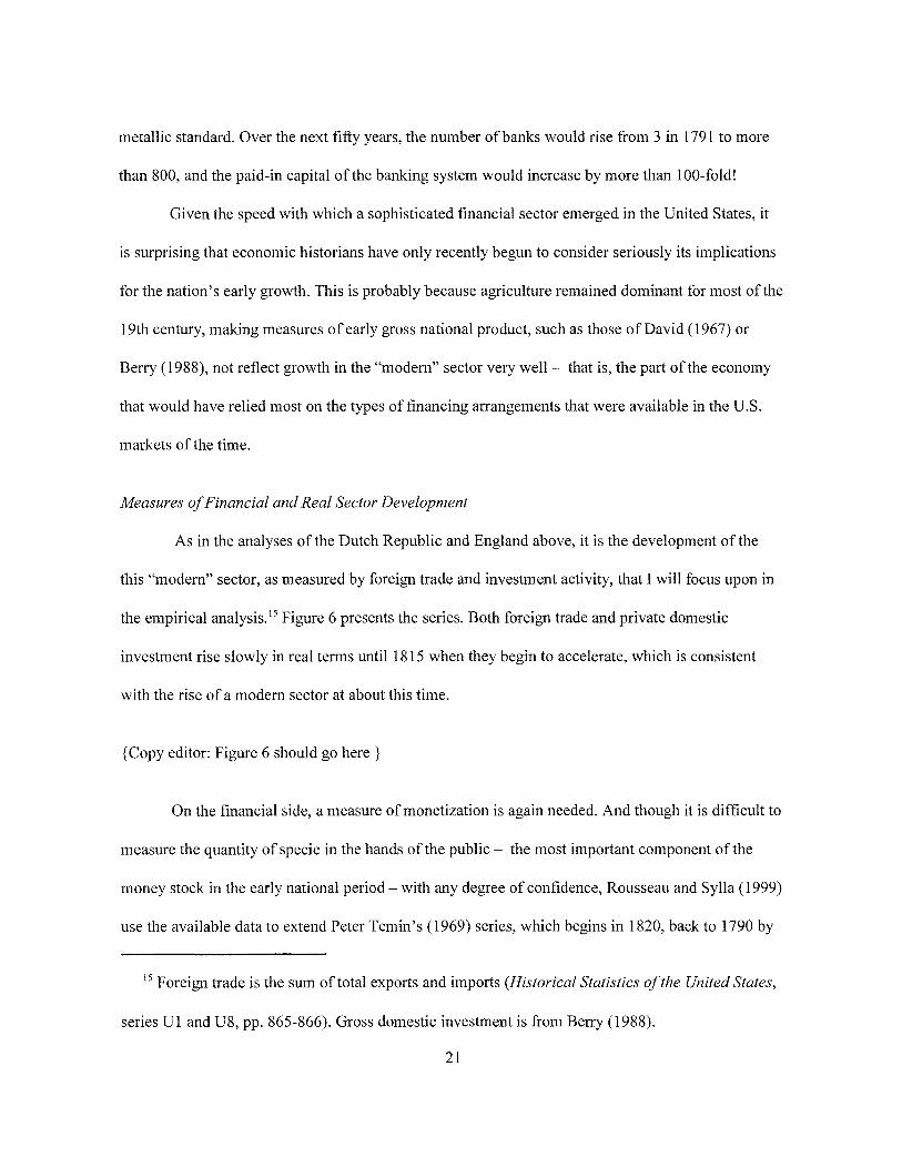
Measures ofFinancial and Real Sector Development

As in the analyses ofthe Dutch Republic andEngland above, it is the development of the

this “modern” sector, as measured by foreign trade and investment activity, that I will focus upon in

the empirical analysis.’5 Figure 6 presents the series. Both foreign trade and private domestic

investment rise slowly in real terms until 1815 when they begin to accelerate, which is consistent

with the rise of a modern sector at about this time.

{Copy editor: Figure 6 should go here }

On the financial side, a measure ofmonetization is again needed. And though it is difficult to

measure the quantity of specie in the hands of the public — the most important component ofthe

money stock in the early national period — with any degree of confidence, Rousseau and Sylla (1999)

use the available data to extend Peter Temin’s (1969) series, whichbegins in 1820, back to 1790 by

‘~Foreign trade is the sum of total exports and imports (Historical Statistics ofthe United States,

series Ui and U8, pp. 865-866). Gross domestic investment is from Berry (1988).

21

replicating Temin’s method as closely as possible.’6 The resulting series includes obligations of

banks to the public and specie outside of banks, and thus represent assets that are either acceptable or

quickly convertible for use in market transactions. Increases in the real value of these assets reflect

more widespread use of the market economy, and might be plausibly linked to trade and investment.

It is also for the United States that I can first introduce securities markets explicitly into the

empirics. Rousseau and Sylla (1999, pp. 7-12), in tandem with Sylla, Wilson, and Wright (1997),

collected the total number of securities listed in the financial press for three major cities (New York,

Philadelphia and Boston) around the end of each calendar year from 1790 to 1850, andI will use this

as a robust measure ofthe size (and perhaps the sophistication) of the securities market.

{Copy editor: Figure 7 should go here }

Figure 7 displays financial series. Both money and securities listings grow slowly until about

1815 whenthey begin to rise quickly. Overall, both series grow at an average rate of about 4.5

percent per year, which is higher than the 1.9 percent growth rate of GDP (Berry 1988) and implies

rapid financial deepening.

Time Series Findings

To explore possible links between the financial and real variables described above, I start

with a VAR specification that includes measures of investment, trade, andmonetization. I will then

add the number of listed securities to this system to measure their additional impact. The method of

bringing securities markets into the analysis incrementally is consistent with Levine and Zervos

16 The data and methods used to construct the annual series for the U.S. money stock are

described in detail in Appendix A of Rousseau and Sylla (1999, pp. 48-50), and the series will

appear in the forthcoming millennial edition ofthe Historical Statistics of the UnitedStates.

22

(1998) and Rousseau and Wachtel (2000), who keep a measure ofliquid liabilities in their baseline

model to allow for complementarities between banks and stock markets in the growth process. All

data are transformed into logs before analysis. Table A. 1 in the Appendix shows that the four series

that I use are statistically indistinguishable from unit root processes, and Table A.2 shows that the

two systems are cointegrated, whichjustifies running the VARs in levels form.

{Copy editor: Table 5 should go here }

Table 5 presents the results. In the upper panel, the findings for the three-variable system

show that the money stock Granger-causes both real investment (top line, third column) at the 2

percent level, and the value of real trade (second line, second column) at the 1 percent level. Trade

Granger-causes investment at the 10 percent level, but has a negative overall effect, which suggests

that increases in the import component oftrade may have to some degree crowded out investment

out in the earlyUnited States. In the lower panel, the results for the four-variable system are similar

to the three-variable results insofar as the monetary effects are concerned, yet the size of the

securities market also exerted a positive and independent effect on investment. Listed securities do

not Granger-cause trade, however, which suggests that the rise of securities markets hadtheir largest

effects in the domestic capital market.

{Copy editor: Figure 8 should go here }

Figure 8 presents selected impulse responses from the four-variable system in Table 5. In

panels (a) and (b), respectively, 1 percent increases in the real stock of money are associated with

increases in trade of 2.78 percent and in investment of 1.35 percent after five years. Panels (c) and

(d) indicate that 1 percent increases in the number of listed securities increase trade by 2.70 percent

23

and investment by 1.37 percent after five years. The result for the effect of listed securities on trade

is striking because the Granger tests did not show a significant effect, which once again is an

important reason to consider the non-linear and interactive impulse responses when evaluating VAR

systems. The effects of both the money stock and the number of listed securities on trade and

investment are of about the same order ofmagnitude once theyhave had an opportunity to work their

way through the VAR for five years. Thus, even though the financial variables yield different

response patterns over time, they are equally as important in fostering commerce and capital

accumulation.

There is no doubt that the data that are available for the United States in the early national

period are sketchy, yet theyhave been generated usingthe bestpractices available to the economic

historian. And the relative strength of the results with these data reveal that the nascent “finance-led

growth” hypothesis for the United States at the very least requires much more investigation among

macro economists and economic historians alike.

JAPAN

Financial Developments in the MeUi Period

In the decade that followed the restoration ofthe Meiji regime in 1868, Japan made a

quantum leap in the development of financial markets and foreign trade, and quickened the pace of

its industrialization. Scholars of the period such as Ott (1960) and Lockwood (1968) have remarked

that the financial sector was instrumental in promoting the adoption of new agricultural and

machine-based industrial technologies that allowed Japan to achieve modern rates ofeconomic

growth after 1885. This section reviews the empirical evidence for this proposition using available

historical statistics and drawing from the more extended analysis in Rousseau (1999).

Among the financial innovations ofthe 1870’s, the most important was the commutation of

24

rice payments (i.e., taxes) that were normally made to the feudal nobility through an issue of long-

term government bonds which were redeemable only at heavy discounts. In an action reminiscent of

Alexander Hamilton, an 1876 revision ofthe National Bank Act then allowed these bonds to be used

as banking capital. Like its U.S. predecessor, stock markets emerged in Tokyo and Osaka shortly

thereafter for trading the fresh securities. A rapid expansion in the number ofnational banks from 5

in 1876 to 151 in 1879 also ensued (Bank of Japan, 1966, p. 196). Among the new banks was the

Yokahoma Specie Bank, which started up in 1880 to meet the foreign exchange needs ofmerchants

who were active in the nation’s growing foreign trade and spurred by the low tariffrates that

remained in effect until 1895. As the economy opened more and more to the West, it was able to

import industrial technologies such as the power loom that had been available in Europe andthe

United States for decades, and was able to do so at relatively low cost.

Japan’s financial development was briefly short-circuited in 1880 when note issues ofthe

newly-formed banks flooded the market and caused an episode of sharp inflation, but this experience

led to a consolidation ofnote issuance under the nation’s first central bank, which formed in 1882. In

short, by 1885 Japan had achieved all five elements ofa “good” financial system, and did so almost

as quickly as the United States had 80 years earlier.

Evidence ofFinance-Led Growth in MeUi Japan

The statistical analysis uses a broad measure of financial development that encompasses the

total assets of Japan’s most important intermediaries and the book values of corporate debt and

equity in the hands ofthe public. The intermediaries include commercial banks (national, private and

ordinary), special banks, savings banks, agricultural cooperatives and insurance companies, but do

not include quasi-banks, small credit cooperatives, and country pawnbrokers who according to

25

Goldsmith (1983, p. 27) accounted for as much as 18 percent of all intermediary assets.’7 Figure 9

shows the remarkable growth of the broad financial aggregate from 1880 to 1913, and contrasts it

with the relative flatness of the amount of currency in circulation, Gross national product and private

domestic fixed investment serve as measures ofreal sector performance.

{Copy editor: Figure 9 should go here }

The tn-variate VAR specifications that I consider include currency in circulation, the broad

financial aggregate, and either output or private fixed investment, with all variables converted to logs

of real 1900 quantities prior to analysis. The unit root and cointegration tests for these systems,

reported in Tables A.1 and A.2 ofthe Appendix, suggest that estimation in levels is appropriate.

Table 6 presents the results. In the top line of the upper panel, financial assets Granger-cause GNP at

the 1 percent level, currency Granger-causes GNP at the 10 percent level, and there is no feedback

from output to either currency or financial assets. The lower panel reports qualitatively similar

findings when private fixed investment replaces output as the measure of real sector activity, except

that investment and financial assets now Granger-cause currency. This result reflects a

complementarity between cash and real investment, which is consistent with the developing-

economy model introduced by McKinnon (1973, esp. chapter 6). There is again no feedback from

investment or currency to financial assets.

{Copy editor: Figure 10 should go here }

17 The source data used to build the financial and real aggregates are from the Bank ofJapan

(1966), Ott (1960), and a five-volume series edited by Ohkawa et al. titled Estimates of the Long-

Term Economic Statistics ofJapan Since 1868. See Rousseau (1999, pp. 196-197) for details.

26

The impulse responses Figure 10 indicates that the effects of real financial assets on real

output and investment are large, with a 1 percent increase in financial assets associated with a 1.38

percent increase in output (panel b) and a 1.37 percent increase in investment after five years (panel

d). It is the effect of currency on investment in panel (c) that is truly striking, with a 1 percent

increase in currency raising investment by 7.6 percent after five years. Though strong inferences

should surely be avoided given the sheer size ofthe response and the fact that it was derived from a

VAR system with only 34 usable time series observations, the result nonetheless emphasizes that all

economic actors did not necessarily have access to the formal financial sector, and may have used

cash as a vehicle for saving to overcome investment indivisibilities.

Overall, the findings for Meiji Japan suggest that financial system played a key role in

promoting output and investment, and offer strong support for the hypothesis of “finance-led”

growth.

FROM 1850 TO THE PRESENT

The case approach taken in the previous sections facilitated the statistical investigation of

four of history’s “financial revolutions” and their impact on real activity, but are indeed limited to

countries that achieved some degree of what might be called economic “success.” This means that

there are elements of selection bias in the cases considered here, not the least of which involves the

very availability ofearly economic data for countries where financial institutions emerged in

conjunction with modernization.

This problem is present but less severe after 1850, however, because economic data become

available for an increasing number of countries. From 1850 to 1929, for example, continuous

measures ofreal output and monetization can be assembled for a set of 17 countries that are often

referred to as the “Atlantic” economies, even though Australia and Japan is usually included in the

27

group.’8 This sample is broad enough to consider a cross-section analysis of the relationship

between financial deepening and economic growth with the techniques used so successfully for the

post World War II period by Ross Levine and his collaborators (e.g., King and Levine, 1993). In this

section, I present a few cross-sectional results for the Atlantic economies over the 1850-1997 period,

and then compare the findings with those obtained for the subperiod from 1850 to 1930.’~

The data are from four main sources. From 1960, it is the World Bank’s World Development

Indicators database. Data for earlier years are from worksheets underlying Bordo and Jonung (2001)

and Obstfeld and Taylor (2000), and Mitchell’s (1998a, 1998b, 1998c).2°

To examine the partial correlations between the size of the financial sector and economic

growth from 1850 while retaining the widest cross section possible, it is necessary to choose a broad

aggregate such as the ratio ofthe liquid liabilities to output as the measure of financial development.

Liquid liabilities is of course an imprecise measure because ofnonbank intermediaries such as

insurance and investment companies whose liabilities do not wind up in the aggregate. These

omissions are probably not that important in the prewar period, but quite substantial in recent years.

Further, the broadly-defined money stock does not include securities markets. Growth in real

income per head, despite its inability to reflect the distribution of wealth and its implications for

18 The seventeen countries are Argentina, Australia, Brazil, Canada, Denmark, Finland, France,

Germany, Italy, Japan, the Netherlands, Norway, Portugal, Spain, Sweden, the United Kingdom, and

the United States.

~ The results draw primarily from Rousseau and Sylla (2001). Interested readers should see this

earlier paper for a more extended analysis.

20 Rousseau and Sylla (2001, pp. 39-45) include a complete description ofthe data sources and

methods used in constructing this panel.

28

welfare, is a common measure ofeconomic performance and is readily available for all seventeen

countries back into the mid- 19th century.

{Copy editor: Table 7 should go here }

Following the now-standard cross-country growth specification ofBarro (1991) as

supplemented by King and Levine (1993), Table 7 presents regressions in which the average growth

rate of real per capita GDP is the dependent variable. Averaging is done across decades for 1850-

1997 period and across five-year periods for 1850-1929. The baseline regression also conditions on

the level of per capita income (in 1960 U.S. dollars) at the start of each period to capture a

convergence or “catching up” effect. The ratio of government expenditure to GDP also appears

because the resource requirements that are often associated with large public expenditures are likely

to “crowd out” private investment and lead to less efficient resource allocations than the private

sector might provide. Finally, the ratio of the broad money stock to GDP is included to capture the

effects of financial development. The specification also includes dummy variables for each time

period to control for time trends in the levels variables and for business cycle effects.

In the OLS regressions, the first observations for each period are used as the regressors to

ameliorate the impact of possible reverse causality from growth to additional finance. This technique

cannot fully eliminate the simultaneity problem due to autocorrelation in the time series for financial

depth, but it does ensure that all regressors are predetermined and thus plausible determinants of

subsequent growth. The IV specifications use contemporaneous averages of the data as regressors

and control for simultaneity by instrumenting in each period with the initial values ofthe complete

set ofregressors, initial inflation, and the ratio ofinitial trade (exports plus imports) to GDP.

A strong convergence effect, as indicated by negative coefficients on initial income that are

29

statistically significant at the 5 percent level, is common to all four regressions reported in Table 7.

Government expenditure has the expected negative sign and is significant at the 5 percent level for

the full 1850-1997 period, but is not quite significant at the 10 percent level for the pre-Depression

period, though the coefficients are about the same size throughout. The coefficient sizes are robust to

the choice of the initial value OLS or IV estimation technique. It is the differences across subperiods

in the coefficients on the ratio ofthe broad money stock, however, that are particularly interesting.

For 1850-1997, the coefficient is about 1 and significant at only the 10 percent level. Evaluated at the

sample mean of 50.6 percent, this implies that an increase in financial depth of 10 percentage points

would increase the annual growth rate of GDP by about 0.1 percent, which is not particularly large.

For the 1850-1929 period, the coefficient is significant at the 5 percent level and more than double

the size, implying an increase in GDP growth of 0.22 percent per year for a ten percentage point

increase in financial depth from the sample mean of 42.8 percent.

The sharper increase in output for a given change in financial depth in the pre-1930 period is

consistent with the view that financial factors matter most emphatically in the early stages of

economic development by mobilizing and allocating resources, and make smaller contributions to

the efficiency of resource allocation in more mature economies. The sample of “Atlantic” economies

makes this point clear, since many were relatively “immature” in the 19th centuryyet nearly all

could be termed “mature” today. King and Levine (1993) obtain results using a similar specification

for the post-1960 period that are similar to mine for 1850-1929, andnow we can posit at least one

reason for this — the King and Levine sample, due to its inclusion of 80 or more countries, captures

many of them in their emerging phases, and is thus closer in composition, at least insofar as phases

ofeconomic development are concerned, to the earlier sample ofAtlantic economies.

30

CONCLUSION

The case studies considered in this article offer statistical evidence that the development of

banking and securities markets mattered for industrialization and the expansion of commerce in four

economies that are generally considered to have experienced “financial revolutions” over the past

400 years. The data are more limited than those at the disposal ofthe modern macro economist, and

this means that results must be interpreted as more suggestive than definitive, yet the consistency of

the evidence with the historical narrative that can be obtained by letting the data speak is

unmistakable. Cross-country evidence for the period from 1850 to the present indicates that the

results obtained in the case studies are not just a result ofbiases imposed by the availability of

historical data.

Surely other factors, and particularly the adoption of new technologies, are also at the center

of commercial and industrial revolutions. In 17th century Amsterdam, that innovation was the ability

to build seaworthy vessels quickly and cheaply enough to exploit the trade opportunities associated

with circumventing the Cape of Good Hope. For early 19th century England, it was steam, the power

loom and a host of other machines that raised productivity. Even in these cases, however, the new

technologies needed financing to get off the ground, andthe emerging financial markets in these

nations seem to have provided it. And the very availability of financing would have encouraged other

potential entrepreneurs to formulate new business ideas.

It is this way that I believe the financial sector mobilized the resources needed to start large

projects in the pre-Industrial period and had incentive effects in the real sector that extended beyond

those firms that actually received financing. It remained for the later industrial phases, at least in

England and the United States, for the financial sector to develop the sophisticated screening and

monitoring functions required to affect economic growth through the quality of resource allocations,

31

but the expansion of deposit banking in these countries ultimately did this as well. The process of

market emergence and expansion prepared each of the four nations for world economic leadership

over the next century — positions that Amsterdam and England were able to retain until new

technologies, both real and financial, displaced them in classic episodes of Schumpeterian creative

destruction. Will today’s information technology revolution hasten the emergence of a “world”

financial market in which the United States will assume the role of partner among equals rather than

the leadership position to which we have grown accustomed over the past century or so?

32

REFERENCES

Bagehot, Walter. Lombard Street.’ A Description ofthe Money Market. New York: Scribner,

Armstrong & Co., 1873.

Barro, Robert J. “Economic growth in a cross section of countries.” Quarterly Journal ofEconomics

(May 1991) 56 (2), pp. 407 -443.

Berry, Thomas Senior, “Production and Population Since 1789: Revised GNP Series in Constant

Dollars.” Bostwick Paper No. 6. Richmond VA: The Bostwick Press, 1988.

Bordo, Michael D., and Lars Jonung. “A Return to the Convertibility Principle? Monetary and Fiscal

Regimes in Historical Perspective,” in A. Leijonufvud (ed.), Monetary Theory as a Basisfor

Monetary Policy. London: Macmillan, 2001.

Brainard, William C., and James Tobin. “Pitfalls in Financial Model Building.” American Economic

Review, May 1968, 58 (2), Papers and Proceedings, pp. 99 - 122.

Bruijn, J. R., F. S. Gaastra, and I. Schoffer. Dutch-Asiatic Shipping in the 17th and 18th Centuries, 3

volumes. The Hague, 1987.

Cameron, Rondo. “England, 1750-1844,” in R. Cameron, 0. Crisp, H. T. Patrick, and R. Tilly, eds.,

Banking in the Early Stages ofIndustrialization: A Study in Comparative EconomicHistory. New

York: Oxford University Press, 1967, pp. 15 - 59.

Chaudhuri, K. N. The Trading World ofAsia and the English East India Company 1660-1760.

Cambridge, UK: Cambridge University Press, 1945.

Clapham, J. H. “The Private Business ofthe Bank ofEngland, 1744-1800.” Economic History

Review, February 1941, 11(1), pp. 77 - 89.

Clapham, J. H. The Bank of England: A History. New York: Macmillan, 1945.

Crafts, N. F. R., Leybourne, S. J., and T. C. Mills. “Trends and Cycles in British Industrial

33

Production, 1700-1913.” Journal ofthe Royal Statistical Society. SeriesA (Statistics in Society),

1989, 152 (1), pp. 43 -60.

David, Paul, “The Growth of Real Product in the United States Before 1840: New Evidence,

Controlled Conjectures.” Journal ofEconomic History, March 1967, 27 (1), pp. 151 - 197.

Davis, Lance E. “The Investment Market, 1870-1914: The Evolution of a National Market.” Journal

of EconomicHistory, September 1965, 25 (3), pp. 355 - 399.

de la Vega, Joseph. Confusion de Confusiones, translated and with an introduction by Hermann

Kellenbenz. Amsterdam: 1688; reprinted Boston: Harvard Graduate School ofBusiness

Administration, 1957.

Dehing, Pit, and Marjolein ‘t Hart. “Linking the Fortunes: Currency and Banking, 1550-1800,” in M.

‘t Hart, J. Jonker, and J. L. Van Zanden, eds., A Financial History ofthe Netherlands. Cambridge:

Cambridge University Press, 1997, pp. 37 - 63.

Dillen, J. G. van. “Effectenkoersen aan de Amsterdamsche Beurs, 1723-1794.” Economische-

HistorischeJaarboek, 1931, l’7,pp. 1-46.

Dillen, J. G. van. “The Bank of Amsterdam,” in J. G. Van Dillen, ed., History of the Public Banks,’

Accompaniedby Extensive Bibliographies ofthe Histories ofBanking and Credit in Eleven

European Countries. The Hague: M. Nijhoff, 1934, pp. 79 - 123.

Fazzari, Steven M., R. Glenn Hubbard and Bruce C. Petersen. “Financing Constraints and Corporate

Investment.” Brookings Papers on Economic Activity, 1988, 1, pp. 141 - 195.

Glamann, Kristof. Dutch-Asiatic Trade, 1620-1 740. Copenhagen: The Danish Science Press, 1958.

Goldsmith, Raymond W. The Financial Development ofJapan, 1868-1977. New Haven: Yale

University Press, 1983.

Greenwood, Jeremy, and Bruce D. Smith. “Financial Markets in Development, and the Development

34

of Financial Markets.” Journal ofEconomic Dynamics and Control, January 1997, 21(1), pp. 145

- 181.

Gurley, John G., and Edward S. Shaw. “Financial Aspects ofEconomic Development.” American

Economic Review, September 1955, 45 (3), pp. 515 - 538.

Huffrnan, Wallace E., and James R. Lothian. “Money in the United Kingdom, 1833-80.” Journal of

Money, Credit and Banking, May 1980, 12(1), Part 1, pp. 155- 174.

Johansen, Soren. “Estimation and Hypothesis Testing of Cointegration Vectors in Gaussian Vector

Autoregressive Models.” Econometrica, November 1991, 59 (6), pp. 1551 - 1580.

Levine, Ross. “Financial Development and Economic Growth: Views and Agenda.” Journal of

Economic Literature, 1997, 35, pp.688-726.

Levine, Ross, and Robert G. King. “Finance and Growth: Schumpeter Might Be Right.” Quarterly

Journal ofEconomics, August 1997, 108 (3), pp. 717 - 738.

Levine, Ross, and Sara Zervos. “Stock Markets, Banks, and Economic.” American Economic

Review, June 1998, 88 (3), pp. 537 - 558.

Lockwood, W. W. The Economic Development ofJapan.’ Growth and Structural Change. Princeton:

Princeton University Press, 1968.

McKinnon, Ronald I. Money and Capital in Economic Development. Washington DC: The

Brookings Institution, 1973.

Mitchell, B. R. British Historical Statistics. Cambridge: Cambridge University Press, 1988.

Mitchell, B. R. International Historical Statistics.’ Africa, Asia and Oceania, 1750-1993. 4th Edition.

New York: Stockton Press, 1998 (a).

Mitchell, B. R. International Historical Statistics.’ The Americas, 1750-1993. 4th Edition. New York:

Stockton Press, 1998 (b).

35

Mitchell, B. R. International Historical statistics: Europe, 1750-1993. 4th Edition. New York:

Stockton Press, 1998 (c).

Neal, Larry. The Rise ofFinancial Capitalism.’ International Capital Markets in the Age ofReason.

Cambridge, MA: Cambridge University Press, 1990.

Obstfeld, Maurice, and Alan M. Taylor. Global Capital Markets: Integration, Crises, and Growth.

Japan-U.S. Center Sanwa Monographs on International Financial Markets. Cambridge:

Cambridge University Press, 2000.

Ohkawa, K., N., M. Shinohara and M. Umemura (eds.), Estimates ofLong-Term Economic Statistics

ofJapan Since 1868, Vols. 1-5. Tokyo: Toyo Keizai Shimposha, 1974.

Osterwald-Lenum, Michael. “A Note with Fractiles of the Asymptotic Distribution ofthe Maximum

Likelihood Cointegration Rank Test Statistics: Four Cases.” Oxford Bulletin of Economics and

Statistics, August 1992, 54 (4), pp. 461- 478.

Ott, DavidJ. Thefinancial development ofJapan, 18 78-1958. Ph.D. dissertation, University of

Maryland, 1960.

Pressnell, L. S. Country banking in the industrial revolution. Oxford, UK: Clarendon Press, 1956.

Richards, R. D. “The First Fifty Years of the Bank of England,” in J. G. Van Dillen, ed., History of

the Public Banks; Accompanied by Extensive Bibliographies ofthe Histories of Bankingand

Credit in Eleven European Countries. The Hague: M. Nijhoff, 1934, pp. 201 - 272.

Rousseau, Peter L. “The Permanent Effects of Innovation on Financial Depth: Theory and U.S.

Historical Evidence from Unobservable Components Models.” Journal ofMonetary Economics,

October 1998, 42 (2), pp. 387 - 425.

Rousseau, Peter L. “Finance, Investment, and Growth in Meiji-Era Japan.” Japan and the World

Economy, April 1999, 11(2), pp. 185 - 198.

36

Rousseau, Peter L., and Richard Sylla. “Emerging Financial Markets and Early U.S. Growth.” NBER

Working Paper No. 7448, December 1999.

Rousseau, Peter L., and Richard Sylla. “Financial Systems, Economic Growth, and Globalization.”

NBER Working Paper No. 8323, June 2001, and forthcoming in M. Bordo, A. Taylor, and J.

Williamson, eds., Globalization in Historical Perspective. Chicago: University of Chicago Press,

2003.

Rousseau, Peter L., and Paul Wachtel. “Equity Markets and Growth: Cross-Country Evidence on

Timing and Outcomes, 1980-1995.” Journal ofBankingand Finance, December 2000, 24 (12),

pp. 1933 - 1957.

Rousseau, Peter L., and Paul Wachtel. “Financial Intermediation and Economic Performance:

Historical Evidence From Five Industrialized Countries.” Journal ofMoney, Credit and Banking,

November 1998, 30 (4), pp. 657 - 678.

Schumpeter, Joseph P. The Theory of EconomicDevelopment. Cambridge, MA: Harvard University

Press, 1911.

Sims, ChristopherA., James H. Stock, and MarkW. Watson. “Inference in Time Series Models With

Some Unit Roots.” Econometrica, January 1990, 58 (1), pp. 113 - 144.

Sylla, Richard. “Federal Policy, Banking Market Structure, and Capital Mobilization in the United

States, 1863-1913.” Journal ofEconomic History, December 1969, 29 (4), pp. 657 - 686.

Sylla, Richard. “U.S. Securities Markets and the Banking System, 1790-1840.” Federal Reserve

Bank ofSt. Louis Review, May/June 1998, 80, pp. 83 - 98.

Sylla, Richard, Jack W. Wilson, andRobert E. Wright. “America’s First Securities Markets, 1790-

1830: Emergence, Development, and Integration.” Paper presented at the Cliometrics Society

Conference, Toronto, Canada, May 1997.

37

Temin, Peter. The Jacksonian Economy. New York: W. W. Norton and Company, 1969.

U.S. Bureau of the Census. Historical Statistics ofthe UnitedStates:from Colonial Times to 1970.

Washington, DC: Government Printing Office, 1975.

van der Wee, H. The Growth ofthe Antwerp Market. The Hague: M. Nijhoiff, 1963.

World Development Indicators. Database. Washington, DC: The World Bank, 1999.

Zanden, Jan Luiten van. “What Happened to the Standard of Living Before the Industrial

Revolution? New Evidence from the Western Part ofthe Netherlands.” Working Paper, 2000.

38

APPENDIX. Time Series Properties of Data Used in the Empirical Analysis

This section presents Augmented Dickey-Fuller (ADF) tests for unit roots and Johansen

(1991) tests for cointegration in the series and VAR systems used in the analysis. If ADF tests are

unable to reject the unit root for a series in levels, yet reject after differencing, there is some

justification for treating the series as 1(1) in subsequent modeling. The univariate representations for

the ADF tests include four lags. The trending nature of the series make both constant and trend

terms necessary in the levels tests, while a constant-only regression is used for the first differences.

The log transformation is applied to series that enter VAR systems as such. Table A. 1 reports the test

statistics and significance levels.

{Copy editor: Table A.1 should go here }

A VAR system with non-stationary variables is classified as cointegrated if a linear

combination exists which yields a stationary series when applied to the data. In the tn-variate case, a

cointegrating relationship also implies that the error terms of the system are stationary. The

technique developed by Johansen (1991) provides a regression-based test for determining both the

presence of cointegration and the number of linear stationary combinations which span the space.

Each system is modeled as a VAR ofthe form

Ax1 = + ~ F1Ax,~+ HxIk + e1, (A.1)

where x1 is a vector containing the potentially endogenous variables and k is adequately large both to

capture the short-run dynamics ofthe underlying VAR and to generate residuals that approximate the

normal distribution. The lag order for each system is chosen with a series of nested likelihood ratio

tests. The presence of trends in the data suggest the inclusion ofan unrestricted intercept. The

Johansen methodology tests whether the H matrix in (B.1) is ofless than full rank via the trace and

maximum eigenvalue statistics. Table A.2 includes the results and significance levels for the four

39

counties in the study.

{Copy editor Table Al should go hat }

40

Tab

le1

VA

Rm

odel

sof

fina

ncia

lqua

ntiti

esan

dV

OC

activ

ity,A

mst

erda

m16

41-

1794

Eq.

Mkt

.va

lue

BA

draw

ing

VO

Cm

oney

Adj

.R2

Eq.

I/V

OC

BA

draw

ing

VO

Cm

oney

Adj

.R2

VO

Ctr

ade

bala

nces

expo

rts

voya

ges

bala

nces

expo

rts

la0.

402

0.20

40.

134

0.66

3la

0.40

50.

245

0.01

10.

340

(0.000)

(0.007)

(0.061)

(0.003)

(0.082)

(0.228)

lb0.

041

0.79

90.

061

0.80

6lb

0.09

70.

778

0.06

20.

809

(0.662)

(0.000)

(0.373)

(0.268)

(0.000)

(0.303)

ic-0

.032

0.31

80.

795

0.69

3ic

0.43

80.

163

0.73

30.

701

(0.551)

(0.010)

(0.000)

(0.119)

(0.043)

(0.000)

Eq.

Mkt

.va

lue

VO

Ctr

ade

BA

draw

ing

bala

nces

VO

Cde

btat

BA

Adj

.R2

Eq.

#V

OC

voya

ges

BA

draw

ing

bala

nces

VO

Cde

btat

BA

Adj

.R2

la0.

420

(0.0

08)

0.39

7(0

.02

1)0.

046

(0.4

66)

0.31

5la

0.69

1(0

.000

)0.

195

(0.0

00)

-0.0

54(0

.463

)0.

718

lb0.

218

(0.0

94)

0.72

9(0

.000

)0.

185

(0.0

46)

0.79

1lb

0.13

2(0

.037

)0.

791

(0.0

00)

0.01

9(0

.271

)0.

794

ic-0

.031

(0.141)

0.05

9(0.056)

0.84

0(0.000)

0.86

8lc

-0.0

06(0.012)

0.04

0(0.118)

0.86

6(0.000)

0.87

3

NO

TE

:E

quat

ion

num

bers

corr

espo

ndto

thos

ein

the

text

.E

ach

VA

Rus

esth

ree

lags

.The

VA

Rs

inth

eup

per

pane

lsar

ein

real

log

leve

ls;

inth

elo

wer

pane

lthe

yar

ein

real

leve

lsdu

eto

zero

valu

esfo

rVO

Cde

btin

som

eye

ars.

The

tabl

ere

port

sth

esu

mof

the

regr

essi

onco

effi

cien

tsfo

rea

chva

riab

lebl

ock,

with

the

sign

ific

ance

leve

lof

the

F-te

stfo

rG

rang

erno

n-ca

usal

ityin

pare

nthe

ses

bene

ath

the

coef

fcie

ntsu

ms.

The

depe

nden

tvar

iabl

esfo

requ

atio

ns(I

a),

(1b)

,an

d(1

c)ar

eth

ere

spec

tive

colu

mn

head

ings

from

left

tori

ght.

For

exam

ple,

inth

eV

AR

repo

rted

inth

eup

per

left

pane

l,th

ede

pend

entv

aria

ble

for e

quat

ion

(la)

isth

em

arke

tva

lue

ofV

OC

trad

e;th

eto

talo

fBan

kof

Am

ster

dam

draw

ing

acco

untb

alan

ces

isth

ede

pend

entv

aria

ble

fore

quat

ion

(1b)

;V

OC

expo

rts

ofha

rdm

oney

isth

ede

pend

ent

vari

able

in(i

c).

41

N

Tab

le2

VA

Rm

odel

sof

Qan

din

vest

men

t,D

utch

Eas

tInd

iaC

ompa

ny17

23-1

794

Eq.

Mkt

.va

lue

BA

draw

ing

VO

CQ

Adj

.R2

Eq.

#V

OC

BA

draw

ing

VO

CQ

Adj

.R2

_____

VO

Ctr

ade

bala

nces

voya

ges

bala

nces

la0.

399

-0.2

110.

062

0.46

7la

0.11

1-0

.103

0.05

00.

032

(0.001)

(0.178)

(0.004)

(0.786)

(0.812)

(0.098)

lb-0

.088

0.413

0.029

0.296

lb0.054

0.477

0.015

0.323

(0.826)

(0.000)

(0.438)

(0.642)

(0.000)

(0.549)

lc-0

.004

-0.2

850.

972

0.89

2lc

0.11

4-0

.080

0.96

40.

897

(0.590)

(0.661)

(0.000)

(0.638)

(0.583)

(0.000)

Eq.

Mkt

.va

lue

VO

Ctr

ade

VO

Cde

btat

BA

VO

CQ

Adj

.R2

Eq.

#V

OC

voya

ges

VO

Cde

btat

BA

VO

CQ

Adj

.R2

la0.

060

(0.9

42)

0.34

3(0

.532

)1.

680

(0.0

55)

0.05

5la

0.30

3(0

.013

)-0

.399

(0.1

26)

0.74

8(0

.000

)0.

550

lb-0

.103

(0.1

35)

0.78

2(0

.000

)0.

097

(0.7

60)

0.82

7lb

0.01

5(0

.027

)0.

866

(0.0

00)

-0.0

45(0

.884

)0.

829

lc-0

.021

(0.5

17)

-0.0

32(0

.709

)0.

973

(0.0

00)

0.89

1ic

0.00

9(0

.335

)-0

.021

(0.3

35)

0.93

8(0

.000

)0.

899

See

note

for

Tab

le1.

43

Table 3VARs of financial and real activity, England 1728-1850

Eq. Industrial Market value Bank of England Adjustedproduction index trade liabilities

la 0.980 -0.025 0.102 0.976(0.000) (0.111) (0.136)

lb 0.054 0.924 0.041 0.938(0.335) (0.000) (0.346)

lc -0.010 0.125 0.888 0.921(0.995) (0.091) (0.000)

Eq. Industrial Market value Bank of England Adjustedproduction index trade private loans R2

la 0.988 0.066 -0.009 0.976(0.000) (0.039) (0.280)

lb 0.075 0.918 0.009 0.938(0.204) (0.000) (0.389)

ic -0.152 0.386 0.877 0.886(0.346) (0.005) (0.000)

Note: See note to Table 1. The VARs use four lags that were selected with

nested likelihood ratio tests. Data are in real log levels.

44

Table 4VAR models ofQ and trade, British East India Company 1710-1745

Eq. Market value EIC EIC Q Adjusted______ EIC trade total debt R2

la 0.979 -0.804 0.382 0.591(0.090) (0.3 86) (0.042)

lb 0.423 0.077 -0.089 0.770(0.004) (0.636) (0.131)

lc -0.069 0.117 0.449 0.653(0.149) (0.254) (0.000)

Eq. Market value EIC EIC Q Adjusted______ EIC trade cash balance R2

la 0.344 -0.241 0.399 0.550(0.388) (0.783) (0.073)

lb -0.590 -0.335 0.057 0.012(0.198) (0.441) (0.965)

Ic -0.513 -0.491 0.567 0.891(0.151) (0.191) (0.000)

Note,’ See note for Table 1. The VARs use three lags. EIC trade and debt are in

real log levels in the upper panel. Due to negative observations for cash, EICtrade

and cash balances enter the VAR in the lower panel as real levels.

45

Table 5VARs of financial and real activity, United States 1790-1850

Eq. Investment Market value Money stock No. listed Adjustedtrade securities R2

hi 0.717 -0.266 0.423 0.964(0.000) (0.094) (0.018)

lb -0.239 0.377 0.549 0.663(0.799) (0.001) (0.010)

ic 0.154 0.037 0.840 0.973(0.075) (0.958) (0.000)

Eq. Investment Market value Money stock No. listed Adjustedtrade securities R2

la 0.245 -0.253 0.28 1 0.470 0.972(0.570) (0.025) (0.009) (0.005)

lb -0.050 0.373 0.597 -0.185 0.664(0.918) (0.001) (0.004) (0.391)

lc 0.089 0.032 0.823 0.074 0.97 1(0.168) (0.961) (0.000) (0.669)

ld -0.053 -0.013 -0.015 1.042 0.991(0.772) (0.879) (0.662) (0.000)

Note: See note to Table 1. The VARs use four lags that were selected with nested

likelihood ratio tests. Data are in real log levels. The lower panel reports results from a

four-dimensional system, which requires an extra equation (1 d) in the VAR.

46

Table 6VARs of financial and real activity, Japan 1880-1913

Eq. GNP Currency in Financial Adjustedcirculation assets R2

la -0.163 0.097 0.360 0.988(0.582) (0.088) (0.001)

lb -0.287 0.800 0.075 0.833(0.576) (0.000) (0.286)

ic -0.170 -0.041 0.999 0.994(0.959) (0.875) (0.000)

Eq. Private Currency in Financial AdjustedInvestment circulation assets R2

la 0.236 1.895 0.457 0.957(0.074) (0.055) (0.036)

lb -0.138 1.060 0.087 0.872(0.010) (0.000) (0.014)

ld -0.080 0.143 1.007 0.993(0.616) (0.585) (0.000)

Note: See note to Table 1. The VAR with GNP uses three lags of each

variable, and the VAR with private investment uses four, with the lag

orders selected with nested likelihood ratio tests.

47

Table 7Cross-Country Growth Regressions, 1850-1997 and 1850-1929

Dependent variable: % Growth of per capita real GDP

1850- 1997 1850 - 1929

OLS IV OLS IV

Constant 7.463” 6.776** 6.206” 6.308””(1.500) (1.477) (2.034) (2.050)

Log of initial real -0.706”’ -0.603”’ ~0.710** ~0.73l**per capita GDP (0.179) (0.179) (0.307) (0.305)

Initial ratio of broad 0.949’ 0.956* 2.2Sf” 2.186**moneytoGDP (0.541) (0.540) (1.075) (1.039)

Initial ratio government -5.280” ~5.915** -6.229 -6.397expenditure to GDP (2.299) (2.583) (3.848) (4.150)

R2 .339 .372 .137 .147(No. observations) (211) (197) (186) (185)

Note.’ The table reports coefficients from OLS and IV regressions with standard errors in

parentheses. The dependent variable is the growth rate ofreal per capita GDP averaged for each

decade for the regressions that cover 1850 to 1997, and averaged over 5-year periods for the

regressions that cover 1850 to 1929. Initial values are taken from the first year of each period.

Period dummies are included in the regression but are not reported. * and * * denote statistical

significance at the 10 percent and 5 percent levels respectively.

48

Amsterdam 1641-1 794

Market value of VOC trade

No. of outbound VOC voyages

VOC hard money exports

BA drawing balances

VOC debt at the BA

England 1728-1850

Industrial production

Market value of trade

BE circulation and deposits

BE private loans

EIC exports (1710-1745)

EIC debt (1710-1745)

EIC cash balances (1710-1745)

EIC Q (1710-1745)

UnitedStates, 1790-1850

Domestic investment

Foreign trade

Money stock

Number of listed securities

Japan, 1880-1913

Gross national product

Private domestic investment

Currency in circulation

Financial assets

-0.10

-0.86

-2.15

-1.41

-2.93

-2.14

-2.52

-3.10

-2.50

-2.14

-2.38

-1.58

1st Difference

~8.60**

-8.46””

-6.48””

-6.36””

~5.29’

-6.85””

-5.94””

~6.09**

-5.35””

_3.19*

-2.48

~3.23”””

-2.88

-4.32””

~4•39*

-3.65”

-3.61”

Table A.l

ADF tests for series used in the empirical analysis

Levels

-2.38

-3.46”

-1.89

-2.85

-3.41

-2.27 ~6.39**

-1.94 -5.42””

-2.68 ~4.67**

-3.80”” _3.68**

In the table, * and ** denote rejection ofthe unit root hypothesis at the 10% and 5% levels.

49

Table A.2

Johansen tests for cointegration

Trace Max. Eigenvalue

r=0 r<l r=0 r 1 r 2

Amsterdam (K = 3)

trade, BA balances, money exports 49.19”” 21.38** 27.81”” 18.16** 3.22*

trade, BA balances, VOC debt 49.03** 11.68 37,35** 9.04 2.64

voyages, BA balances, money exports 55~74** 27.05”” 28.69** 24.20** 2.58

voyages, BA balances, VOC debt 46.90** 21.12** 25.78** 18.04** 3.08*

trade,BAbalances,VOCQ 38.22** 12.17 26.05”” 11.12 1.05

trade, VOC debt, VOC Q 33.63** 8.37 25.26”” 7.11 1.26

voyages, BA balances, VOC Q 35.53”” 14.89” 18.63” 15.95** 0.94

voyages, VOC debt, VOC Q 26.92” 8.64 16.29 7.36 1.27

England (K = 4)

industrial prod., trade, BE liabilities 33.53”” 14.05” 19.48” 9.76 4.29”

industrial prod., trade, BE loans 23.93 7.38 16.55 4.16 3.22

EIC trade, EIC debt, EIC Q (K 3) 45.01”” 19.37** 25.63** 13.92* 545**

EIC trade, EIC cash, EIC Q (K = 3) 41.84** 20.19”” 21.65”” 14.39”” 5.81””

UnitedStates (K = 4)

investment, trade, money 34.24** 6.05 28.19** 5.80 0.25

investment, trade, money, #secs 60.23”” 20.93 8.76 39.30”” 12.17 7.83

r<4 0.93

Japan (K = 4)

GNP, currency, financial assets 3777** 9.01 25.76 6.31 2.70

investment, currency, financial assets 48.52** 9.45 39.07”” 6.20 2.70

K is the lag at which the levels terms enter the test regressions. The columns labeled r=0 test a nullhypothesis of no cointegration, while the r 1 (r 2) columns test a null of at most one (two)cointegrating vectors. * and * * denote rejections ofthe null at the 10% and5% levels respectively,withcritical values from Osterwald-Lenum (1992), Table 1.

50

51

52

1640 1660 1680 1700 1720 1740 1760 1780 18000

5

10

15

20

25

30

35

VOC Trade

BA Balances

Money Exports

VOC Debt at BA

Figure 1. Finance and Trade Quantities, Amsterdam, 1641-1794.

53

Year 1 3 5 7 9 11 13 15

-0.1

0

0.1

0.2

0.3

0.4

0.5

0.6 Effect of BA Balances on VOC Trade

Year 1 3 5 7 9 11 13 15

-0.1

0

0.1

0.2

0.3

0.4

0.5

0.6 Effect of BA Balances on VOC Voyages

Year 1 3 5 7 9 11 13 15

-0.1

0

0.1

0.2

0.3

0.4

0.5

0.6 Effect of Money Exports on VOC Trade

Year 1 3 5 7 9 11 13 15

-0.20

0.20.40.60.8

11.21.4 Effect of BA Balances on Money Exports

(a) (b)

(c) (d)

Figure 2. Selected impulse responses from VARs for Amsterdam, 1641-1794.

Note: The impulse responses are taken from the VARs reported in the upper panels of Table 1. Each

plot traces the percent change in the affected variable that results over a fifteen-year horizon from a 1

percent change in the orthogonalized innovation to the potentially causal variable. The ordering is BA

balances first, VOC hard money exports second, and either the market value of VOC trade or the number

of VOC voyages third. Using Monte Carlo integration, the solid lines are the mean responses that result

from 10,000 random draws from the distribution of the estimated VAR coefficients. The dotted lines are

one standard error bands.

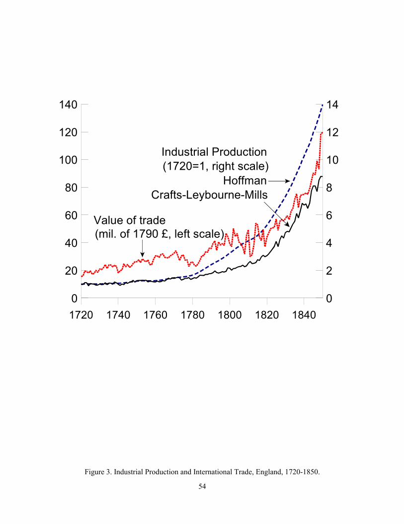
54

1720 1740 1760 1780 1800 1820 18400

20

40

60

80

100

120

140

0

2

4

6

8

10

12

14

Industrial Production

Value of trade (mil. of 1790 £, left scale)

(1720=1, right scale)Hoffman

Crafts-Leybourne-Mills

Figure 3. Industrial Production and International Trade, England, 1720-1850.

55

1725 1745 1765 1785 1805 1825 18450

10

20

30

40

50

60

0

50

100

150

200

250M2 (right scale)

BE Private Loans (left scale)

BE Circulation and Deposits (left scale)

Figure 4. Monetary Aggregates, England, 1728-1850.

56

Year 1 3 5 7 9 11 13 15

-0.2

0

0.2

0.4

0.6

0.8

1 Effect of BE Liabilities on Industrial Production

Year 1 3 5 7 9 11 13 15

-0.2

0

0.2

0.4

0.6

0.8

1 Effect of Industrial Production on Trade

Year 1 3 5 7 9 11 13 15

-0.1

-0.05

0

0.05

0.1 Effect of BE Private Loans on Trade

Year 1 3 5 7 9 11 13 15

-0.2

0

0.2

0.4

0.6

0.8

1 Effect of BE Liabilities on Trade

(a) (b)

(c) (d)

Figure 5. Selected impulse responses from VAR systems for England, 1728-1850.

Note: The impulse responses are taken from the VAR systems reported in Table 3. The ordering places

BE deposit and circulation liabilities or BE private loans first, the real market value of trade second, and

real industrial production third. Using Monte Carlo integration, the solid lines are the mean impulse

responses that result from 10,000 random draws from the posterior distribution of the estimated VAR

coefficients. The dotted lines are one standard error bands.

57

1790 1800 1810 1820 1830 1840 18500

100

200

300

400

500

Private Domestic

Market value of trade

Investment

Figure 6. Private Investment and Foreign Trade, United States, 1790-1850.

58

1790 1800 1810 1820 1830 1840 18500

100

200

300

400

500

Money Stock

Number of Securities Listed

(mil. of 1840 U.S. $)

In Three Cities

Figure 7. Monetary and Financial Aggregates, United States, 1790-1850.

59

Year 1 3 5 7 9 11 13 15

-0.6

-0.2

0.2

0.6

1

1.4

1.8 Effect of Money on Trade Value

Year 1 3 5 7 9 11 13 15

-0.6

-0.2

0.2

0.6

1

1.4

1.8 Effect of Money on Investment

Year 1 3 5 7 9 11 13 15

-0.6

-0.2

0.2

0.6

1

1.4

1.8 Effect of Securities Listings on Trade

Year 1 3 5 7 9 11 13 15

-0.6

-0.2

0.2

0.6

1

1.4

1.8 Effect of Securities Listings on Investment

(a) (b)

(c) (d)

Figure 8. Selected impulse responses from 4-variable VAR for the United States, 1790-1850.

Note: The impulse responses are taken from the VAR systems reported in the lower panel of Table 5.

The variable ordering places the number of listed securities first, the real money stock second, the real

market value of trade third, and real investment last. Using Monte Carlo integration, the solid lines plot

the mean impulse responses that result from 10,000 random draws from the posterior distribution of the

estimated VAR coefficients. The dotted lines are one standard error bands.

60

1880 1885 1890 1895 1900 1905 19100

0.5

1

1.5

2

2.5

3

3.5

4

4.5

Currency in Circulation

Financial Assets

Figure 9. Monetary and Financial Aggregates, Japan, 1880-1913.

61

Year 1 3 5 7 9 11 13 15

-0.6

-0.4

-0.2

0

0.2

0.4

0.6 Effect of Currency on GNP

Year 1 3 5 7 9 11 13 15

-0.1

0

0.1

0.2

0.3

0.4

0.5 Effect of Financial Assets on GNP

Year 1 3 5 7 9 11 13 15

-3-2-1012345 Effect of Currency on Private Investment

Year 1 3 5 7 9 11 13 15

-1

-0.5

0

0.5

1

1.5

2

2.5 Effect of Financial Assets on Private Investment

(a) (b)

(c) (d)

Figure 10. Selected impulse responses from VARs for Japan, 1880-1913.

Note: The impulse responses are taken from the VARs reported in Table 6. The variable ordering places

financial assets first, currency second, and either GNP or private domestic investment third. Using

Monte Carlo integration, the solid lines plot the mean impulse responses that result from 10,000 random

draws from the distribution of the estimated VAR coefficients. The dotted lines are one standard error

bands.