Hindcasts of tropical Atlantic SST gradient and South American

precipitation: the influences of the ENSO forcing and the Atlantic

preconditioning

Huei-Ping Huang1,*

, Andrew W. Robertson2, Yochanan Kushnir

3, Shiling Peng

4

1 Department of Mechanical and Aerospace Engineering, Arizona State University2 International Research Institute for Climate and Society, Columbia University

3Lamont-Doherty Earth Observatory of Columbia University

4 NOAA ESRL/Physical Science Division and CIRES, University of Colorado

Revised, October 2008

*Corresponding author address: Department of Mechanical and Aerospace Engineering,

Arizona State University, Tempe AZ 85287-6106 e-mail: hp.huang@asu.edu

1

Abstract

Hindcast experiments for the tropical Atlantic sea surface temperature (SST) gradient, G1,

defined as tropical North Atlantic SST anomaly minus tropical South Atlantic SST anomaly, are

performed using an atmospheric general circulation model coupled to a mixed-layer ocean over

the Atlantic to quantify the contributions of the El Nino-Southern Oscillation (ENSO) forcing

and the preconditioning in the Atlantic to G1 in boreal spring. The results confirm previous

observational analyses that in the years with a persistent ENSO SST anomaly from boreal winter

to spring, the ENSO forcing plays a primary role in determining the tendency of G1 from winter

to spring and the sign of G1 in late spring. In the hindcasts, the initial perturbations in Atlantic

SST in boreal winter are found to generally persist beyond a season, leaving a secondary but

non-negligible contribution to the predicted Atlantic SST gradient in spring. For 1993-94, a

neutral year with a large pre-existing G1 in winter, the hindcast using the information of Atlantic

preconditioning alone is found to reproduce the observed G1 in spring. The seasonal

predictability in precipitation over South America is examined in the hindcast experiments. For

the recent events that can be validated with high-quality observations, the hindcasts produced

dryness in boreal Spring 1983, wetness in Spring 1996, and wetness in Spring 1994 over

northern Brazil that are qualitatively consistent with observations. An inclusion of the Atlantic

preconditioning is found to help the prediction of South American rainfall in boreal spring. For

the ENSO years, discrepancies remain between the hindcast and observed precipitation

anomalies over the northern and equatorial South America, an error that is partially attributed to

the biased atmospheric response to ENSO forcing in the model. The hindcast of the 1993-94

neutral year does not suffer this error. It constitutes an intriguing example of useful seasonal

forecast of G1 and South American rainfall anomalies without ENSO.

2

1. Introduction

The research in the predictability of tropical Atlantic meridional SST gradient has a long

history since early studies suggested its potential influences on the rainfall anomaly over the

Nordeste (northern Brazil) region of South America (e.g., Nobre and Molion 1988, see the

survey in Uvo et al. 1998). Using station data for precipitation, previous observational analyses

(e.g., Giannini et al. 2004) showed that, in boreal spring, the Nordeste region tends to be drier

than normal with a positive Atlantic SST gradient, G1 (defined as tropical North Atlantic SST

anomaly (tNA) minus tropical South Atlantic SST anomaly (tSA)), because a warmer than

normal tNA or a colder than normal tSA drives the Atlantic ITCZ northward, away from the

Nordeste. (See Fig. 1 and caption for definitions of tNA and tSA boxes.) Conversely, a negative

G1 implies wetness over northern Brazil. This suggests the possibility of incorporating the

prediction of G1 in the practical prediction of the rainfall anomalies over South America.

Among the two components of SSTs that define G1, tNA is known to be more strongly

influenced by ENSO and is positively correlated with the NINO3 SST index (e.g., Enfield and

Mayer 1997, Alexander and Scott 2002, Huang et al. 2005a), while tSA is recognized as being

regulated by local internal variability (e.g., Chang et al. 1998, Czaja et al. 2002, Barreiro et al.

2004, 2005, Trzaska et al. 2007). Thus, G1 tends to have the same sign as the NINO3 index in

the boreal spring of "year 1" (the year that follows the December peak of an El Nino or La Nina)

of a strong ENSO event after the influence of ENSO on the Atlantic is fully established. Using

the observation from 1876-1997, Huang et al. (2005a) clarified that about two-third of the strong

ENSO events are concordant, in the sense (as envisioned by Giannini et al. 2004) that G1 in

boreal spring has the same sign as the NINO3 index averaged from the preceding winter to early

spring. The other one-third are discordant, for which the ENSO forcing from boreal winter to

3

spring is not sufficient to overturn a pre-existing Atlantic SST gradient such that G1 and NINO3

have opposite signs in spring. In the discordant cases, tSA in boreal spring can often be tracked

back to a strong pre-existing SST anomaly in the central South Atlantic in the preceding boreal

winter (Huang et al. 2005a, Barreiro et al. 2004). Figure 1, adapted from Huang et al. (2005a),

illustrates the composites of the SST anomalies for the (a) concordant, and (b) discordant cases,

and (c) the typical precondition for the latter. Following previous work (Giannini et al. 2004,

Huang et al. 2005a), the two boxes in Fig. 1a are chosen to define the tNA and tSA used in this

study. Based on the observational analysis, G1 in boreal spring should generally depend on the

ENSO forcing from boreal winter to spring and the preconditioning in the Atlantic SST in boreal

winter. In this study, we will use a series of GCM hindcast experiments to assess the

contributions of these two components to the seasonal predictability in the Atlantic SST and in

the precipitation over South America.

We will analyze the behavior of the simulated SST anomalies in ensemble hindcast

experiments using an atmospheric GCM partially coupled to a mixed-layer ocean model for the

Atlantic. The experimental design is described in Section 2. The results of the model

simulations of the Atlantic SST and SST gradient are discussed in Section 3. In addition to the

SST, the model predicted precipitation anomalies will be analyzed in Section 4 in the context of

the relationships among the Atlantic SST gradient, ENSO forcing, and South American rainfall

anomalies. Concluding remarks follow in Section 5.

2. The model and numerical experiments

2a. Selection of cases

We will focus on selected years with the combinations of one or more of the following

4

conditions: (i) Persistent ENSO forcing from late boreal winter to boreal spring; (ii) A strong

preconditioning in the Atlantic SST in boreal winter; (iii) A large tendency or strong persistence

in G1 from late boreal winter to boreal spring. These criteria are quantified by the monthly

NINO3 and G1 indices as shown in Fig. 2. They are detrended with a 10-year high pass filter in

the same manner as in Huang et al. (2005a). (The observed SST anomalies used in the initial

condition of our hindcast experiments and those used for model verification are also pre-

processed in the same way.) of the the Each grid box represents one month and each row in one

of the panels in Fig. 2, from left to right, represents one year, defined as July of one year (called

"year 0") to June of the following year (called "year 1"), with time increasing downward from

1947 to 1997 (the top row is July 1947-June 1948, bottom row is July 1996-June 1997.) Note

that the color interval, shown at bottom, for G1 is only on-third of that for NINO3. Visually, the

right panel looks noisier than the left panel; The NINO3 index exhibits a greater degree of

month-to-month persistence. However, the persistence of NINO3 is stronger in the first half

(from boreal summer of yr 0 to boreal winter of yr 0/1) of the ENSO year, leaving us a reduced

number of cases with the desired condition of a persistent ENSO forcing from boreal winter to

spring of yr 1, the time of year when G1 is important. Among these cases, a few are found to

have a large tendency (large increase or decrease during the season) or strong persistence in G1

from boreal winter to spring. They are selected for our hindcast experiments as marked by the

arrows in Fig. 2. They include two ENSO warm events (1968-69, 1982-83) and three cold

events (1970-71, 1988-89, 1995-96). In addition, we selected a neutral year of 1993-94 that is

distinguished by a strong preconditioning in winter and strong persistence of G1 from winter to

spring. We have chosen the cases from the last 30 years of the 20th century for which there are

more high-quality observational data (for Atlantic SST and precipitation) available to validate

5

the hindcast.

The cases chosen are listed in Table 1. The majority of the ENSO events in that list are

concordant, i.e., the G1 index in late boreal spring has the same sign as the NINO3 index

averaged from late boreal winter to boreal spring. In most of them, G1 changes sign from

positive in late boreal winter to negative in late boreal spring for ENSO cold events, and from

negative to positive for ENSO warm events. This is expected, as we have chosen the cases with

strong ENSO in boreal winter-spring. They correspond to (by the ENSO-tNA connection, see

section 3) the cases with the largest tendency in G1 from late boreal winter to late boreal spring,

thus the likelihood of having G1 chaning sign over that period. These cases are chosen because

the large seasonal tendency in G1 makes it easier to interpret the results of our numerical

experiments. The cases with G1 having the same sign through the boreal winter-spring season

(which can be either concordant or discordant, the latter is mostly associated with weak ENSO

events, see Huang et al. 2005a) are weak ENSO or neutral events. They are not chosen because,

in the observation (to be used to verify the hindcast), the weak seasonal tendency in G1 in these

cases is more easily overwhelmed by the sub-seasonal variability in G1, rendering it difficult to

verify and interpret the ENSO-induced tendency in the hindcast. (See section 2b for the setup of

the hindcast experiments.) Otherwise, we have evenly sampled ENSO warm and cold events

that are known to exhibit some degree of asymmetry in their remote atmospheric responses (e.g.,

Sardeshmukh et al. 2000).

2b. The model and experimental design

The hindcast model is a T42 28-level version of the National Center for Environmental

Prediction (NCEP) atmospheric GCM (close to the 2001 version of the "MRF" model) coupled

6

to a mixed layer ocean over the Atlantic. The mixed layer model consists of a 50 m slab ocean

with "flux correction" similar to that in Peng et al. (2006) but without the Ekman transport, as

detailed in Appendix A. Although the atmosphere-ocean coupling is relatively simple, there is

evidence from previous studies that thermodynamic coupling alone is useful for the seasonal

prediction of Atlantic SST anomalies (e.g., Giannini et al. 2004, Saravanan and Chang 2004). In

multi-year test runs with climatological SST imposed outside the Atlantic, climate drift in SST is

found to be small within the coupled domain. In the hindcast experiment we will use the model

simulated SST minus the observed climatological SST to define the SST anomaly to be

compared to observation. The domain for the mixed layer ocean model is from 50S to 36N over

the Atlantic, as shown in Figs. 4-7. The entire South Atlantic is included because we are

interested in the preconditioning in boreal winter in the South Atlantic (see Fig. 1c). Additional

remarks on the detail of the mixed layer model are in Appendix A.

Each hindcast run is a one-year integration starting from a generic September 1 initial state

for the atmosphere. An ensemble of 25 runs for each case are constructed by randomly

perturbing the mid-tropospheric divergence field in the atmospheric initial condition. The

atmospheric model is integrated for 2 months uncoupled and forced with climatological SST,

and then coupled to the mixed-layer model on November 1 when an observed SST anomaly is

imposed in the initial condition over the coupled domain. The coupled model is then integrated

forward to August of year 1. For most cases, we will focus on the results from November of

year 0 to June of year 1. Because the observed Atlantic SSTs have only monthly (or weekly in

selected recent times) resolution, the "initial state" of SST on November 1 used in our simulation

is actually taken from the average of the monthly means of October and November of the

selected year.

7

A prototypical outcome of a prediction run with a 3-member ensemble shown in Fig. 3

serves to illustrate the behavior of the coupled model. To construct a meaningful example, the

SST anomaly in the initial state in the Atlantic on November 1 is constructed from the composite

of seven cases (see figure caption) that have a large, positive, SST anomaly over the South

Atlantic box in Fig. 1c. Imposing the composite SST anomaly for the Atlantic in the initial

condition, the three runs are performed with the climatological SST imposed outside the coupled

domain. The simulated daily SST anomalies averaged over the South Atlantic box are shown in

Fig. 3 with the individual ensemble members in color and the ensemble mean in black. Although

the switch-on of coupling and the addition of the initial perturbation in the SST on November 1

is rather abrupt, Fig. 3 shows that, after a brief initial drop in amplitude, the model retained a

substantial fraction of the initial perturbation and allowed it to persist into the boreal spring of

year 1. The filled and open circles show the monthly means of the simulated (ensemble mean)

and observed (composite of the 7 selected years) SST anomalies for the South Atlantic box from

November to June. The SST anomaly drops off more quickly in the model than in the

observation but the former still has an e-folding time longer than a season.

Three types of runs are performed for each of the selected cases described in Section 2a.

The "Initial Condition Only" (IC Only) runs are similar to the example in Fig. 3 and are

performed with the observed SST anomaly imposed in the initial (November 1) state but with the

seasonally varying climatological SST imposed outside the coupling domain. The "ENSO

forcing Only" (ENSO Only) runs are without any initial SST perturbation on November 1 but

with the observed SST anomaly over the tropical Pacific (165E-90W, 15S-15N) added to the

imposed climatological SST outside the coupling domain. The ENSO+IC runs have both ENSO

forcing from the Pacific and the initial perturbation in the SST over the Atlantic. (For the ENSO

8

Only and ENSO+IC runs, during the first two months the ENSO forcing in the Pacific is already

turned on.) Unless otherwise noted, each type of runs consists of a 25-member ensemble of one-

year integration (i.e., total of 75 runs for each of the ENSO events described in Section 2a). In

addition, a 25-member "control run" is performed with no ENSO forcing and no initial

perturbation (but with coupling turned on) on November 1. This set of runs will be used to

define the simulated precipitation anomalies in Section 4. Table 1 summarizes the major

hindcast runs performed for this study.

3. Hindcast of SST

3a. Hindcast of Atlantic SST

Figures 4a and 4b show the observed SST anomalies over the Atlantic in November 1968

and April 1969. Figures 4c-4e show the ensemble mean of the SST anomalies in April 1969 from

the hindcast runs with IC only, IC+ENSO forcing, and ENSO forcing only. The shaded areas are

with above 95% statistical significance, based on the signal-to-noise ratio estimated from the

ensemble mean and the intra-ensemble standard deviation. In the observation, tSA is initially

positive while tNA is slightly negative in November 1968. The gradient, G1 = tNA-tSA,

increases to a positive value in April 1969 due to the warming in tNA, a canonical response to

the positive ENSO forcing from boreal winter to spring (e.g., Huang et al. 2005a). This is

captured by the hindcast runs with ENSO+IC (Fig. 4d) and ENSO Only (Fig. 4e). In the IC Only

runs (Fig. 4c), the SST anomaly in the South Atlantic in April retains the structure of the initial

state in November. However, in North Atlantic, the initial SST anomaly in November decays to

nearly zero in April. These results suggest that, in the model runs, tNA in boreal spring was

controlled primarily by the ENSO forcing from boreal winter to spring, while tSA was

9

influenced by the persistence of the preconditioning in the preceding winter.

Figure 5 is similar to Fig. 4 but for the 1970-71 case (Figs. 5b-5e are for April 1971), an

ENSO cold event in which tNA turned from nearly neutral in November to cold in April (Figs.

5a and 5b). The initially positive tropical Atlantic SST gradient is reversed to negative in spring.

This is captured by the hindcast runs with ENSO+IC or ENSO Only, although the model

simulations produced too-cold SST anomalies over equatorial Atlantic and tropical South

Atlantic. In the IC Only runs, the pattern of SST anomaly in the South Atlantic persisted while

that in the tropical North Atlantic dissipated to nearly zero, a behavior similar to the 1968-69

case (Fig. 4c). In the ENSO Only runs, the response in the tropical South Atlantic is very weak.

Again, in this case, the simulated tNA is dominated by ENSO forcing while tSA is determined

by the persistence of the pre-existing anomaly in winter.

Figure 6 shows the observation and hindcast for the 1982-83 case (Figs. 6b-6e are for

April 1983), a strong ENSO warm event. In this case, the response in tNA is canonical; It turns

from negative in November (Fig. 6a) to strongly positive in April (Fig. 6b). The close

resemblance of Figs. 6d and 6e indicates that the response in spring in the ENSO+IC runs is

dominated by the ENSO forcing. In the model, the SST response to ENSO forcing in the

equatorial Atlantic and tropical South Atlantic is positive enough (Fig. 6e) to overwhelm a

negative SST anomaly from the persistence of the initial condition as inferred from the IC Only

runs (Fig. 6c), resulting in a net positive response in the ENSO+IC runs opposite to that

observed. Nevertheless, the positive response in tNA is strong enough that the model still

predicted a positive G1 in spring, qualitatively consistent with that observed. The errors in the

simulated equatorial Atlantic SST could be related to the omission of ocean dynamics in the

ocean model. In addition, the excessive warming over the tropical Atlantic in the ENSO+IC and

10

ENSO Only runs may also be attributed in part to the model bias in the atmospheric response to

Pacific ENSO forcing. As discussed in Appendix B, the model response in the tropical

tropospheric temperature over the Atlantic sector is too strong (too warm during El Niño and too

cold during La Niña) compared to observation.

The results for the other three cases are shown in an abridged fashion in Fig. 7 with the

left and middle columns the observed SST anomalies in November of yr 0 and April of yr 1, and

the right column the simulated SST anomaly in April of yr 1. The hindcast in the right column

are from the ENSO+IC runs except for 1993-94 (panel f), which is from the IC Only runs. For

the 1988-89 ENSO cold event, the ENSO+IC runs produced the cooling of tNA in spring but not

as pronounced as that observed. The simulated SST anomalies in the equatorial and tropical

South Atlantic are too cold. This error also occurred in the ENSO Only runs but not in the IC

Only runs (not shown), indicating that it is related to the aforementioned model bias in the

atmospheric response to ENSO. The model still produced the correct sign (negative) of G1 in

boreal spring, due to the simulated substantial cooling in tNA.

The 1993-94 case, middle row of Fig. 7, is unique in that it is an ENSO neutral year

with a very strong preconditioning in the Atlantic. Moreover, the observed pattern of the SST

anomaly persisted from November 1993 to April 1994 for almost the entire Atlantic domain,

preserving the negative G1 from the initial state. The IC Only hindcast runs correctly produced

the cool tNA, warm tSA, and negative G1 in boreal spring. Since this is a neutral year, the

ENSO+IC runs (not shown) produced similar results as the IC Only runs. With the correct

prediction of the tropical Atlantic SST, in Section 4 we will further demonstrate a useful

prediction in the precipitation over South America from this case.

For the 1995-96 cold event (bottom row of Fig. 7), the ENSO+IC runs simulated the

11

cooling trend from boreal winter to spring in tNA. The simulated cooling is somewhat

excessive, culminating in a negative tNA in April 1996 opposite to that observed. The simulated

SST anomalies in spring are also colder than observed for the equatorial Atlantic and tropical

South Atlantic. This behavior also exists in the ENSO Only runs (not shown). Yet, even in this

case, the model correctly simulated the sign of G1 (negative) in spring as that observed.

A quick conclusion from the above six cases is that the sign of G1 in boreal spring is not

difficult to reproduce in the model simulations. For the ENSO years, this is because the model

correctly simulates the warming or cooling in tNA through the robust ENSO-tNA connection.

The response in tNA is usually strong enough that, even with some errors in tSA and/or the

equatorial Atlantic SST, the sign of G1 in the hindcast can still remain correct. However, the

errors in tSA and equatorial Atlantic SST are not without a consequence. We will show in

Section 4 that they degrade the prediction of precipitation in some areas in South America.

3b. The evolution of tropical Atlantic SST gradient

The behavior of the monthly mean Atlantic SST gradient, G1, is summarized in Fig. 8 for

the (a) 1968-69, (b) 1970-71, and (c) 1993-94 cases. Black, blue, and red indicate the observation

and the hindcast runs with ENSO+IC and IC Only, respectively. The half length of the vertical

bar indicates one (intra-ensemble) standard deviation. For the 1968-69 warm event with an

initially negative G1, without the ENSO forcing the negative G1 persisted into spring (the IC

Only runs). The observed upward trend in G1 and the negative value of G1 in spring are

correctly simulated with the added ENSO forcing, which dominates in this case. The behavior of

the 1970-71 case in Fig. 8b is similar to that of the 1968-69 case but just with a reversal of sign

for the SST anomalies; The IC Only runs simulated persistence of a positive G1 into spring,

12

while the ENSO+IC runs correctly produced the downward trend in G1 and a negative G1 in

spring as that observed. The behavior of G1 for other ENSO years discussed in Section 3a is

qualitatively similar to the above two. For those years, the inclusion of the ENSO forcing is

essential for the prediction of G1 in spring.

An intriguing case in which ENSO forcing does not dominate is 1993-94 , shown in Fig. 8c

(also see Figs. 7d-7f). Since this is a neutral year, the "ENSO forcing" has only a minor

contribution to the prediction of G1 (the difference between the ensemble means of the blue and

red curves in Fig. 8c is not statistically significant at 95% level). In the observation (black), an

initially strongly negative G1 persisted and maintained its amplitude into spring. The IC Only

runs reproduced this persistence although with a greater decay of the amplitude of G1 with time

than that observed. Even so, the predicted G1 in April remains strongly negative.

3c. Further remarks

The results of the hindcast experiments may generally depend on the model and the

manner of atmosphere-ocean coupling. To quickly assess the behavior of our coupled model,

here we compare the ENSO-induced surface fluxes in our simulations to other studies. Figure 9

shows the effect of the ENSO forcing, defined as the difference between the ensemble means of

the ENSO Only and Control runs, on the surface energy fluxes for December-February from

ENSO "warm minus cold" composite (see caption for detail). A positive flux anomaly (red)

indicates an energy flow into the ocean, corresponding to heating in the SST. The ENSO-

induced anomalous latent heat flux (LHF, left) is strongly positive over tNA, the major cause for

the warming there from winter to spring. This is consistent with previous studies (e.g.,

Alexander and Scott 2002). In the Northern Hemisphere, the anomalous long wave (LW,

13

middle) and short wave (SW, right) radiative fluxes as responses to ENSO forcing are generally

weaker than the anomalous LHF. The LW and SW contributions tend to cancel each other. The

SW and LW radiative fluxes in Fig. 9 is somewhat different from that in Alexander and Scott

(2002, using a more sophisticated mixed layer model with vertical variations), in which the

ENSO forcing induces a positive signal in SW and a moderately negative signal in LW over the

tNA region and the Caribbean. In our simulation, the response in the sensible heat flux is

weaker than in the other three components and is not shown. Figure 9 also shows that the

ENSO-induced surface energy flux anomalies are generally stronger in the North than in the

South Atlantic.

In previous studies (e.g., Czaja et al. 2002, Enfield et al. 2006, Lee et al. 2008, and a

review by Kushnir et al. 2006), the evolution of the tNA SST anomaly is sometimes discussed in

connection with the North Atlantic Oscillation (NAO). These studies have focused on the longer

time scales, e.g., the interannual variability of NAO and tNA based on the seasonal mean NAO

and tNA indices. Here, we have not emphasized this connection (although the information of the

phase of NAO is embedded in the initial condition for the tNA SST in our simulations) because

we are concerned with the short term, sub-seasonal, evolution of tNA SST anomalies within a

season. On this shorter time scale, the variability of NAO is not well understood but it has been

shown by recent studies to be largely a manifestation of synoptic weather events with a decaying

time scale of less than 10 days (Feldstein 2000, Benedict et al. 2004). The evolution of the NAO

index on the very short time scale can, then, be viewed as part of the synoptic noise in our

seasonal forecast and needs not be discussed separately. (Moreover, in our hindcast experiment,

this high-frequency noisy component is significantly reduced after averaging the 25 ensemble

members.) On the interannual and longer time scale (as previous studies have investigated),

14

more structured air-sea interaction process involving NAO and Atlantic SST may emerge after

the high-frequency noise is filtered out. Our problem of seasonal forecast lies between these two

extremes but the short-term influence of random synoptic events likely remains important. Thus,

for our current discussion we choose not to further separate NAO from the general short-term,

sub-seasonal noise.

In our analysis we have treated tNA and tSA as separate entities, noting that tNA is

generally more strongly influenced by ENSO and tSA by internal variability. The role of the

cross-equatorial interaction between tSA and tNA in enhancing the persistence (e.g., though

WES feedback, Xie et al. 1999) of both of them is an interesting possibility for further studies.

The persistence of the SST anomalies may also depend on season, another point that can be

further explored by applying our hindcast system to other seasons.

4. Hindcast of precipitation

Since our study of the Atlantic SST gradient is motivated by its potential influence on the

precipitation over northern South America, we will next examine the simulated precipitation

anomalies from the hindcast experiments. The interpretation of the simulated precipitation

anomalies is complicated by the fact that the ENSO forcing not only indirectly influences South

American rainfall by modifying the Atlantic SST gradient but it can also affect the precipitation

through a more direct thermodynamical mechanism (e.g., Chiang and Sobel 2002, and further

interpretation in Huang et al. 2005b). Briefly, a plausible scenario of this direct influence is

related to (consider an ENSO warm event) the eastward spreading of warm tropospheric air

along the equator from the Pacific to the South American and Atlantic sector (Yulaeva and

Wallace 1994, Chiang and Sobel 2002). The resulted warmer air aloft causes an increase in the

15

static stability of the atmosphere over northern South America, thereby a suppression of rainfall

there. Thus, northern South America is dry during El Niño and wet during La Niña. This

mechanism exists in the ENSO+IC and ENSO Only hindcast runs and it is entangled with the

effect of the Atlantic SST gradient in determining the precipitation anomalies over South

America. Only in the "IC Only" runs can we clearly relate the precipitation anomalies to the

Atlantic SST or SST gradient.

Unlike the SST over the coupled domain that is constrained by the flux correction, the

model-predicted precipitation has a more noticeable bias over the tropical Atlantic and South

America. The bias over this region is a common problem for GCMs (e.g., Biasutti et al. 2006).

In boreal spring, our model produced excessive rainfall over the Amazon basin compared to

observation (not shown). To circumvent the problems arising from the precipitation bias, we

define the predicted precipitation anomaly as the difference between the ensemble means of the

25-member hindcast runs and that of another set of 25-member "control runs" (instead of the

observed climatology) that retain the coupling over the Atlantic but not ENSO forcing nor

imposed initial perturbations in the SST.

The observed precipitation anomalies to be used for model validation are constructed

from the daily gridded South American precipitation data set of Liebmann and Allured (2005). A

quality check is performed to exclude the grid points where too few observations (too few days -

usually 10 days as the threshold - per month) are available to robustly defined the climatology

and/or monthly mean anomaly for a particular month. They are left blank in the panels for the

observation shown in Figs. 10-13. We will discuss only the four most recent cases of our

simulations in the post-1980 era, for which the observation of precipitation has the highest

quality.

16

To assess the impacts of the error in the Atlantic SST on the simulated precipitation, we

will further compare our results with a set of nine-member "AMIP" runs - atmospheric GCM

forced by the observed SST - using a GCM similar to our hindcast model (both are the T42 28-

level version of the NCEP atmospheric GCM but the latter is a slightly more recent version).

The model output for the AMIP runs is made available to us through the International Research

Institute for Climate and Society (IRI) Data Library. For the AMIP runs, the precipitation

anomalies are defined as the departure from the long-term mean deduced from the same set of

simulations.

Figure 10 shows the precipitation anomalies for April 1983 from the 25-member ensemble

means of our hindcast runs with (a) ENSO+IC, (b) ENSO Only, and (c) IC Only, all to be

compared to (d) the 9-member ensemble mean of the AMIP runs, and (e) the observation. The

ENSO+IC hindcast runs and the AMIP runs both reproduced the typical dryness over northern

Brazil for this ENSO warm event. The observed wetness over the northern (north of the equator)

South America is partially reproduced by the AMIP runs but is absent in the ENSO+IC runs,

which also produced wetness further north over the Caribbean. In the above comparison, it

should also be noted that the observation in Fig. 10e represents just one realization, in contrast to

the ensemble means in Figs. 10a and 10b. The disagreement in the small-scale structures

between the model and observation may be due to sampling. For this strong El Niño case, the

simulated drying over northern South America is mainly due to the ENSO forcing. The result of

the ENSO Only runs (Fig. 10b) is similar to that of the ENSO+IC runs (Fig. 10a). The IC Only

runs (Fig. 10c) produced overall a weaker response but it nevertheless captures the drying over

Nordeste. The precipitation anomalies in Fig. 10c can be clearly related to the simulated Atlantic

SST anomalies (Fig. 6c). The dipole-like structure (that straddles the equator) in the

17

precipitation anomaly corresponds to a northward shift of ITCZ, consistent with a cool tSA and

positive G1 in Fig. 6c. Incidentally, the precipitation anomalies over the equatorial Atlantic and

the northern tip of South America from the IC Only runs are more consistent with the

observation (and AMIP runs) than those from the ENSO+IC or ENSO Only runs. The latter two

produced excessive drying centered on the equator (vs. south of the equator in the IC Only runs,

AMIP runs, and observation). This is related to the excessive tropical tropospheric warming as

the model bias in the response to El Niño (Appendix B). The effect of the bias somewhat

diminished the benefit of adding the ENSO forcing to the hindcast runs even though the forcing

was shown to help the prediction of tNA. A similar concern about the mixed benefit of the

ENSO forcing for the prediction of remote precipitation anomalies in a coupled model was also

put forth by Misra and Zhang (2007).

Figure 11 is similar to Fig. 10 but for April 1996 from the 1995-96 case, a cold event.

Except for a reversal of sign, the behavior of the observed and simulated precipitation anomalies

in this case is similar to that in Fig. 10. The typical wetness over northern Brazil associated with

a cold event is observed (Fig. 11e) and simulated by the AMIP runs (Fig. 11d). The wetness is

also simulated by the full hindcast (ENSO+IC) runs (Fig. 11a) but it is weaker compared to Figs.

11d and 11e. The IC Only runs (Fig. 11c) also produced wetness over northern Brazil and a hint

of dryness over the northern tip of South America similar to that observed. The result from the

ENSO Only runs (Fig. 11b) is mixed. Except for a small-scale dry stripe located along the north

shore of northern Brazil, the hindcast produced large-scale wetness over most of northern South

America. While this is qualitatively a typical response to La Niña, the simulated wetness was too

wide-spread, for example the northern tip of South America is wet, opposite to that observed.

This may, again, be related to the bias in the model response to ENSO forcing. Figures 11a-11c

18

also demonstrate that linear superposition cannot be applied to the simulated precipitation field;

The sum of the outcomes of the ENSO Only and IC Only runs does not equal that of the

ENSO+IC runs, due to the nonlinear dependence of precipitation on the SST and atmospheric

circulation.

Figure 12 is similar to Fig. 11 but for the neutral year of 1993-94 (shown is April 1994),

and only the IC Only hindcast runs are shown in Fig. 12a. The hindcast with only the

information of the initial SST anomaly in November 1993 produced realistic features in the

precipitation anomaly with wetness over northern Brazil and dryness over the northwestern tip of

South America, similar to that observed (Fig. 12b) and simulated by the AMIP runs (Fig. 12c).

The wetness over northern Brazil and dryness north of it in Fig. 12a can be clearly related to the

cool tNA and warm tSA (and negative G1) in the simulated SST anomalies (Fig. 7f) that also

agree with the observations (Fig. 7e).

Figure 13 is similar to Fig. 12 but for the ENSO cold event of 1988-89 (shown is April

1989), a case in which the full ENSO+IC hindcast runs (Fig. 13a) performed poorly in

reproducing the observed precipitation anomaly (Fig. 13b) over South America. The AMIP runs

(Fig. 13c), on the other hand, reproduced the observed wetness over northern Brazil and dryness

over the northwestern tip of South America. As discussed in Section 3a, for this event, although

the ENSO forcing in the ENSO+IC runs produced the observed cooling trend in tNA and the

correct sign of G1, it also produced excessive and unrealistic cooling in tSA and the equatorial

Atlantic - the sign of the SST anomalies there is the opposite of that observed. In this case, the

negative impact of the latter is substantial enough to render the simulated precipitation anomalies

inaccurate over the aforementioned regions in South America.

Figure 14 shows the root-mean-square error in the model simulated precipitation anomaly

19

for April of year 1 over the pNSA (Northern tropical South America, top panel) and pSSA

(Southern tropical South America, bottom panel) regions as indicated by the red boxes in Fig.

13c. The error is calculated from the difference between the ensemble mean of the model

simulation and the observation (interpolated onto model grid) at every grid point over land

within the box, and is evaluated for the AMIP, ENSO+IC, ENSO Only, and IC Only runs. From

left to right are the three individual ENSO cases, their average, and the neutral case of 1994.

The error over pSSA is generally smaller than that over pNSA. For all ENSO cases, except

pNSA in 1983, the ENSO+IC runs out-perform the ENSO Only runs in predicting the

precipitation anomalies in April. This indicates useful predictability of South American rainfall

embedded in the Atlantic preconditioning.

As a summary, except for the 1988-89 case, we found that the relatively simple

AGCM+ML coupled model qualitatively reproduced the observed dryness or wetness over

northern Brazil south of the equator. For the ENSO years, a greater discrepancy in the

precipitation anomalies between the hindcast runs with ENSO forcing and the observation or

AMIP runs occur over the northern (north of the equator) and equatorial South America and

equatorial Atlantic. This error is attributed in part to the model bias in the atmospheric response

to Pacific ENSO forcing (Appendix B). Note that this negative impact of the ENSO forcing on

the hindcast of South American precipitation does not contradict the positive impact discussed in

Section 3 on the correct simulations of the Atlantic SST gradient, G1. As explained before, for

ENSO years the success of the latter is mainly due to the ability of the model to simulate tNA

through the ENSO-tNA connection. Our results here imply that the precipitation anomalies over

the equatorial South America and equatorial Atlantic depend on more than just tNA and/or the

sign of G1. Interestingly, the hindcast for the 1993-94 case does not suffer the problem of the

20

biased response to ENSO since it is a neutral year with minimal ENSO forcing. It reproduced

both the observed wetness over northern Brazil and the dryness north of it. Moreover, devoid of

the imposed ENSO forcing, the successful IC Only "hindcast" may be regarded as a "forecast",

since in this simulation the predictability of the South American precipitation anomalies in April

1994 is embedded in the initial condition of the SST in November 1993.

5. Concluding remarks

Our analyses of the hindcast experiments indicate that, in the cases with a persistent ENSO

forcing from boreal winter to spring, the forcing is the dominant factor in determining the

evolution of the tropical Atlantic SST gradient, G1, and the sign of G1 in late spring. In the

absence of ENSO forcing, the sign of G1 in boreal winter tends to persist into spring such that

the preconditioning in the Atlantic SST also provides a non-negligible contribution to the overall

value of G1 in spring. This finding confirms the results of previous observational analyses of a

primary role of ENSO but a non-negligible secondary role of Atlantic preconditioning in

determining G1 in boreal spring for ENSO events -- recall the statistics of two-third concordant

vs. one-third discordant in Huang et al. (2005a). In most cases our hindcast runs with ENSO+IC

correctly simulated the sign of G1 in late spring. For the ENSO years, this success is mainly due

to the correct simulation of tNA due to its clear connection to ENSO forcing.

The majority of our hindcast runs also simulated reasonable precipitation anomalies over

northern Brazil south of the equator, although for ENSO years a larger discrepancy is found

between the simulated and observed precipitation anomalies over the northern and equatorial

South America and equatorial Atlantic. This is attributed in part to the model bias in the

atmospheric response to ENSO forcing. For the ENSO events, the ENSO+IC runs generally out-

21

perform the ENSO Only runs in predicting the rainfall anomalies over the northern half of South

America, indicating predictability of South American rainfall embedded in the Atlantic

preconditioning. While there is still room for improvement for our model given its biased

response to ENSO forcing, the results of this study at least demonstrated that a correct simulation

of tNA and the sign of G1 alone does not sufficiently lead to an accurate simulation of the

rainfall anomalies over the equatorial South America and the northern South America. The

improved simulations for these regions by the AMIP runs indicate that accurate information in

tSA and the equatorial Atlantic SST is needed for the prediction of the precipitation anomalies in

boreal spring in these regions in South America.

The most interesting case of our numerical experiments is the hindcast (essentially

"forecast") for the neutral year of 1993-94, for which the IC Only runs using the observed SST

anomaly in November 1993 produced realistic tropical Atlantic SST gradient and precipitation

anomalies over northern South America in April 1994. The relationship between the simulated

Atlantic SST gradient and South American rainfall anomalies, namely, a negative G1

accompanying the wetness over northern Brazil and the dryness north of it, is consistent with the

canonical picture derived from previous observational analyses. The 1993-94 case presents an

intriguing example of useful seasonal forecast of G1 and South American rainfall anomalies

without ENSO.

Appendix A: Tests for the AGCM+ML model

The mixed layer model consists of a 50 m slab ocean with flux correction. The formula for

flux correction follows Peng et al. (2006) but excludes the Ekman transport effect because our

desired coupling domain includes the equator (in its vicinity the formula for Ekman transport in

22

Peng et al. (2006) becomes singular). As detailed in Peng et al. (2006), the daily climatology of

the SST, TC, was first constructed from the observation. It was used to force a 60-member

ensemble of atmospheric GCM simulations to produce the daily climatology of the (downward)

surface heat flux, QC. The prognostic equation for the SST in the mixed-layer model can be

written in terms of the anomalies of the SST (T) and heat flux (Q),

�T '� t

=Q'

��cpH � , (A1)

where T' = T− TC and Q' = Q − QC are the departure from daily climatology, cp is the heat

capacity of sea water, and H = 50 m is the depth of the mixed layer. In the coupled model, after

(A1) is used to renew T', the total SST is used to force the AGCM. The model is integrated

forward to produce the new Q', and so on. In this study, we have used a constant H = 50 m for

the whole Atlantic Ocean although the model has the option of adopting a more realistic spatially

varying H (for example, the mixed layer depth off the west coast of Africa is generally shallower

than 50 m) in future experiments.

With the constraint of flux correction, the simulated SST does not drift significantly from

the climatological seasonal cycle. Figure A1 shows an example of the SST averaged over the

South Atlantic box shown in Fig. 1c from a 5-yr test run. Black and red are the observed

climatology (repeated for 5 years) and the model simulated SST. The behavior of the simulated

SST over other regions, e.g., the tNA and tSA boxes in Fig. 1a, is similar to that shown in Fig.

A1. The climate drift in the SST is generally small during the first 10 months, the duration of

our coupled hindcast runs.

We have also performed another set of sensitivity test by extending the northern boundary

23

of the mixed layer model from 36ºN to 50ºN for the 1968-69 case. The behaviors of simulated

tNA, tSA, and G1 in boreal spring remain very similar to those from the unmodified case

discussed in the main text.

Appendix B: Atmospheric response to ENSO forcing in the AGCM+ML model

As noted in Section 3-4, the errors in the hindcast of Atlantic SST may be attributed in

part to the model bias related to the atmospheric response to Pacific ENSO forcing. While a

comprehensive diagnosis of the model bias is beyond the scope of this study, we will use the

1982-83 case to illustrate an aspect of this bias and its implications for the simulated Atlantic

SST. We choose to examine this particular year because it has the strongest Pacific ENSO

forcing. Moreover, since the five ENSO warm and cold events we studied each has its own

distinctive life cycle (with their maximum SST anomalies peaking at different times), a

composite of the five events might not necessarily lead to a clearer picture of the bias.

Figure B1a shows the atmospheric response to the Pacific ENSO forcing in the vertically

averaged temperature from our model simulations. The ENSO response is defined as the 25-

member ensemble mean of the ENSO-Only runs for 1982-83 minus the 25-member ensemble

mean of the control runs (forced by climatological SST), both retain the coupling to the mixed

layer model over the Atlantic. The temperature anomaly shown is the average from January-

May 1983 and is the mass-weighted vertical average from the surface to � � 0.1, where � = p/ps

is the terrain-following "sigma" coordinate. Figure B1b is the observational counterpart of B1a,

using the sigma-level (spectral coefficient) data from NCEP reanalysis (Kalnay et al. 1996) and

with the anomaly defined as the departure from the 1979-2003 climatology. As is well-known,

the atmospheric response to a Pacific ENSO SST anomaly generally consists of two components

24

of quasi-stationary wave trains (e.g., Horel and Wallace 1981, Trenberth et al. 1998) and a

zonally symmetric response (e.g., Chiang and Sobel 2002, Robinson 2002, Seager et al. 2003).

The latter is especially prominent in the tropospheric temperature field, with zonal bands of

tropical warming and extratropical cooling accompanying El Niño and the opposite

accompanying La Niña (Yulaeva and Wallace 1994, Seager et al. 2003, Chiang and Sobel 2002).

In Fig. B1, the zonally symmetric response in the tropospheric temperature is stronger in our

simulation than that observed. In the former, the tropical tropospheric warmth spreads eastward

more deeply into the Atlantic sector. In the observation, although there is still a positive

temperature response on the equator, the temperature anomaly is more confined to the west of

the Atlantic sector with the maximum of the temperature anomaly partially blocked by the South

American continent. (An examination of the 1995-96 ENSO cold event revealed a similar

behavior, namely, in the model the ENSO-induced cold equatorial tropospheric temperature

anomaly spreads farther into the Atlantic sector than that observed, causing a cold bias over the

equatorial Atlantic, not shown.) Although many factors could potentially contribute to this bias,

a plausible one is that the Andes mountain range is severely flattened in the model (due to its

relatively coarse T42 resolution), allowing a more thorough eastward intrusion of the tropical

tropospheric warm air into the Atlantic sector. The bias discussed here may contribute to the

errors in the SST over the equatorial Atlantic and in the precipitation over the equatorial South

America and equatorial Atlantic in our hindcast runs with ENSO forcing.

The effect related to the Andes is but one of the plausible explanations for the bias in

tropical tropospheric temperature shown in Fig. B1. For example, using the framework of Gill

(1980) for the linear response of the tropical atmosphere to an ENSO-like SST forcing, it is

known that the ratio of the amplitude of the zonally symmetric to zonally asymmetric

25

temperature response increases with a decreasing damping coefficient (e.g., Gill 1980, Wu et al.

2001, Bretherton and Sobel 2002). The bias of an excessive zonally symmetric warmth induced

by El Niño (coolness induced by La Niña) might also arise from too weak effective damping (by

parameterized boundary layer friction, cumulus friction, etc.) in the tropics in our model. These

possibilities are worth exploring in future work.

Acknowledgment

The authors thank Dr. Brant Liebmann for providing the South American precipitation

data set used in this study. The comments and suggestions from three anonymous reviewers

helped improve the manuscript. This work was supported by NSF grant ATM-05-43256, NOAA

CLIVAR-Atlantic Program, NOAA CPPA Program, and the CICAR award No.

NA03OAR4320179 from NOAA, U.S. Department of Commerce.

References

Alexander, M., and J. Scott, 2002: The influence of ENSO on air-sea interaction in the

Atlantic, Geophys. Res. Lett., 29, 1701, doi:10.1029/2001GL014347

Barreiro, M., A. Giannini, P. Chang, and R. Saravanan, 2004: On the role of the Southern

Hemisphere atmospheric circulation in tropical Atlantic variability, in Earth's Climate: the

ocean-atmosphere interaction, Geophys. Monogr. Ser., vol. 147, edited by C. Wang, S.-P. Xie,

and J. Carton, pp. 143-156, AGU, Washington, D. C.

Barreiro, M., P. Chang, L. Ji, R. Saravanan, and A. Giannini, 2005: Dynamical elements of

predicting boreal spring tropical Atlantic sea surface temperatures, Dyn. Atmos. Oceans,

39, 61-85

26

Benedict, J. J., S. Lee, and S. B. Feldstein, 2004: Synoptic view of the North Atlantic Oscillation,

J. Atmos. Sci., 61, 121-144

Bretherton, C. S., and A. H. Sobel, 2003: The Gill model and the weak temperature gradient

approximation, J. Atmos. Sci., 60, 451-460

Biasutti, M., A. H. Sobel, and Y. Kushnir, 2006: AGCM precipitation biases in the tropical

Atlantic, J. Climate, 19, 935-958

Chang, P., L. Ji, H. Li, C. Penland, and L. Matrosova, 1998: Prediction of tropical Atlantic sea

surface temperature, Geophys. Res. Lett., 25, 1193-1196

Chiang, J. C. H., and A. H. Sobel, 2002: Tropical tropospheric temperature variations caused by

ENSO and their influence on the remote tropical climate, J. Climate, 15, 2616-2631

Czaja, A., P. van der Vaart, and J. Marshall, 2002: A diagnostic study of the role of remote

forcing in tropical Atlantic variability, J. Climate, 15, 3280-3290

Enfield, D. B., and D. A. Mayer, 1997: Tropical Atlantic sea surface temperature variability and

its relation to El Nino-Southern Oscillation, J. Geophys. Res., 102, 929-945

Enfield, D. B., S.-K. Lee, and C. Wang, 2006: How are large western hemisphere warm pools

formed? Prog. Oceanogr., 70, 346-365

Feldstein, S. B., 2000: The timescale, power spectra, and climate noise properties of

teleconnection patterns, J. Climate, 13, 4430-4440

Giannini, A., R. Saravanan, and P. Chang, 2004: The preconditioning role of tropical Atlantic

variability in the development of the ENSO teleconnection: implications for the prediction

of Nordeste rainfall, Clim. Dynam., 22, 839-855

Gill, A. E., 1980: Some simple solutions for heat-induced tropical circulation, Q. J. R. Meteor.

Soc., 106, 447-462

27

Horel, J. D., and J. M. Wallace, 1981: Planetary-scale atmospheric phenomena associated with

the Southern Oscillation, Mon. Weather Rev., 109, 813-829

Huang, H.-P., A. W. Robertson, and Y. Kushnir, 2005a: Atlantic SST gradient and the

influence of ENSO, Geophys. Res. Lett., 32, L20706, doi:10.1029/2005GL023944

Huang, H.-P., R. Seager, and Y. Kushnir, 2005b: The 1976/77 transition in precipitation over the

Americas and the influence of tropical sea surface temperature, Clim. Dynam., 24, 721-740

Kalnay, E., and co-authors, 1996: The NCEP/NCAR 40-year reanalysis project, Bull. Am.

Meteorol. Soc., 77, 437-471

Kushnir, Y., W. A. Robinson, P. Chang, A. W. Robertson, 2006: The physical basis for

predicting Atlantic sector seasonal-to-interannual climate variability, J. Climate, 19,

5949-5970

Lee, S.-K., D. B. Enfield, and C. Wang, 2008: Why do some El Nino have no impact on tropical

North Atlantic SST?, Geophys. Res. Lett., in press

Liebmann, B., and D. Allured, 2005: Daily precipitation grids for South America, Bull. Am.

Meteor. Soc., 86, 1567-1570

Misra, V., and Y. Zhang, 2007: The fidelity of NCEP CFS seasonal hindcasts over Nordeste,

Mon. Weather Rev., 135, 618-627

Nobre, C. A., and L. C. B. Molion, 1988: The climatology of droughts and drought prediction, in

"The impact of climate variations on agriculture: Assessments in semi-arid regions", M. Parry,

T. R. Carter, and N. T. konjin, Eds., Kluwer Academic, pp. 305-323

Peng, S., W. A. Robinson, S. Li, M. A. Alexander, 2006: Effects of Ekman transport on the NAO

response to tropical Atlantic SST anomaly, J. Climate, 19, 4803-4818

Robinson, W. A., 2002: On the midlatitude thermal response to tropical warmth, Geophys. Res.

28

Lett., 29, doi:10.1029/2001GL014158

Saravanan, R., and P. Chang, 2004: Thermodynamic coupling and predictability of tropical sea

surface temperature , in Earth's Climate: the ocean-atmosphere interaction, Geophys.

Monogr. Ser., vol. 147, edited by C. Wang, S.-P. Xie, and J. Carton, pp. 171-180, AGU,

Washington, D. C.

Sardeshmukh, P. D., G. P. Compo, and C. Penland, 2000: Changes of probability associated with

El Nino, J. Climate, 13, 4268-4286

Seager, R., N. Harnik, Y. Kushnir, W. Robinson, J. Miller, 2003: Mechanisms of

hemispherically symmetric climate variability, J. Climate, 16, 2960-2978

Trenberth, K. E., G. W. Branstator, D. Karoly, A. Kumar, N.-C. Lau, and C. Ropelewski, 1998:

Progress during TOGA in understanding and modeling global teleconnections associated with

tropical sea surface temperature, J. Geophys. Res., 103, 14291-14324

Trzaska, S., A. W. Robertson, J. D. Farrara, and C. R. Mechoso, 2007: South Atlantic variability

arising from air-sea coupling: local mechanisms and tropical-subtropical interactions,

J. Climate, 20, 3345-3365

Uvo, C. B., C. A. Repelli, S. E. Zebiak, and Y. Kushnir, 1998: The relationship between tropical

Pacific and Atlantic SST and northeast Brazil monthly precipitation, J. Climate, 11, 551-562

Wu, Z., E. S. Sarachik, and D. S. Battisti, 2001: Thermally driven tropical circulations under

Rayleigh friction and Newtonian cooling, J. Atmos. Sci., 58, 724-741

Xie, S.-P., 1999: A dynamic ocean-atmosphere model of the tropical Atlantic decadal variability,

J. Climate, 12, 64-70

Yulaeva, E., and J. M. Wallace, 1994: The signature of ENSO in global temperature and

precipitation fields derived from the microwave sounding unit, J. Climate, 7, 1719-1736

29

Figure captions

Fig. 1 The composites of the March-May SST anomalies for the (a) concordant, and (b)

discordant, cases for all major ENSO warm events from 1865-2000. A concordant case is

defined as the one in which the tropical Atlantic SST gradient, G1, in March-May has the same

sign as the NINO3 index in the preceding December-January. A discordant case is the opposite.

The composite of the SST anomalies in January-March, i.e., precursor to the SST anomaly in

Fig. 1b, for the discordant cases is shown in (c). The tNA (5N-25N, 60W-30W) and tSA (25S-

5S, 30W-0E) boxes are marked in panel (a). Contour interval is 0.1C, negative dashed. Shading

indicates a high level (> 95%) of statistical significance. Adapted from Huang et al. (2005a).

Fig. 2 The observed monthly-mean tropical Atlantic SST index, G1 (right), and the NINO3

SST index (left panel) for 1948-1997. Each row is a year, defined as July of yr 0 to June of yr 1.

The top row is for July 1947-June 1948 and bottom row July 1996-June 1997. The years

indicated by an arrow are selected for our hindcast experiments. The year indicated at right

corresponds to year 1. The color scales are shown at bottom. Note that the color interval for G1

is one-third of that for NINO3.

Fig. 3 A test run for illustrating the behavior of the hindcast model. Shown are the simulated

daily surface temperature anomalies averaged over the South Atlantic box in Fig. 1c for the

ensemble mean (black) and the individual ensemble members (colored lines) for a set of 3-

member runs. The initial SST perturbation, imposed to the mixed layer model at November 1 of

year 0 (when the coupling is turned on), is constructed from the composite of the average of the

October and November monthly SST anomalies from 1953, 1959, 1969, 1974, 1983, 1988, and

1994. The selected years satisfy the criterion that the SSTA of (October+November)/2 averaged

over the South Atlantic box is greater than 0.3C. The filled and open circles are the simulated

(ensemble mean) and observed (composite of the six selected years) monthly SSTA for the South

Atlantic box.

Fig. 4 The SST anomalies for the 1968-69 case. (a) Observed SSTA in November of yr 0

30

(1968). (b) Observed SSTA in April of yr 1 (1969). (c)-(e) The 25-member ensemble means of

the model simulated SSTA with IC Only (c), ENSO+IC (d), and ENSO Only (e) (See text for

detail). Shading indicates a high level (> 95%, using the ensemble mean anomaly and intra-

ensemble variance to define the signal-to-noise ratio) of statistical significance. The tNA and tSA

boxes are marked in panel (a).

Fig. 5 Same as Fig. 4 but for the 1970-71 case.

Fig. 6 Same as Fig. 4 but for the 1982-83 case.

Fig. 7 Similar to Fig. 4 but for, top to bottom, 1988-89, 1993-94, and 1995-96. The left column

shows the observed SSTA in November of yr 0, middle column the observed SSTA in April of

yr 1, and right column the simulated SSTA from the hindcast experiments. For the 1988-89

(panel c) and 1995-96 (panel i) cases the ENSO+IC runs are shown. For the 1993-94 case, an

ENSO neutral year, the IC Only runs are shown in the right column.

Fig. 8 The observed (black) and model simulated (blue with ENSO+IC, red with IC only)

monthly mean G1 for (a) 1968-69, (b) 1970-71, and (c) 1993-94.

Fig. 9 The ENSO-induced anomalies in the surface latent heat flux (left), long wave radiative

energy flux (middle), and short wave radiative energy flux (right panel) averaged from

December of year 0 to February of year 1 and defined as the difference between the ensemble

means of the ENSO-Only and Control runs. Shown is the ENSO warm minus cold composite,

defined as the average of the two warm events (1968-69, 1982-83) minus the average of the three

cold events (1970-71, 1988-89, 1995-96). Red (positive) means a net energy flux into the ocean,

corresponding to heating in the SST.

Fig. 10 The precipitation anomalies for April 1983. (a) Hindcast with ENSO+IC. (b) Hindcast

with ENSO Only. (c) Hindcast with IC Only. (d) AMIP runs. (e) Observation. (a)-(c) are 25-

member ensemble means from the 1982-83 case. (d) is the 9-member ensemble mean. Color

scale is shown at bottom.

Fig. 11 Same as Fig. 10 but for April 1996 (hindcast runs for the 1995-96 case). (a) ENSO+IC.

31

(b) ENSO Only. (c) IC Only. (d) AMIP runs. (e) Observation.

Fig. 12 The precipitation anomalies for April 1994. (a) Hindcast with IC Only. (b) Observation.

(c) AMIP runs.

Fig. 13 Same as Fig. 12 but for April 1989 (hindcast runs for the 1988-89 case). In panel (c), the

red boxes north and south of the equator over South America indicate the pNSA and pSSA

regions, respectively, used for Fig. 14.

Fig. 14 The root-mean-square error in the precipitation anomaly for April of year 1 averaged

over the pNSA (top panel) and pSSA (bottom panel) regions as defined in Fig. 13c. The error is

calculated from the r.m.s. of the ensemble mean of the hindcast minus observation at every grid

point over land within the box. The errors associated with the AMIP, ENSO+IC, ENSO-Only,

and IC-Only runs are shown in green, red, blue, and gray. The three groups of bars at left are for

the three individual post-1980 ENSO events discussed in the text. The group marked by "AVE"

is the average over the three events. The error for the neutral year 1994 is shown at right.

Fig. A1 The SST averaged over the South Atlantic box in Fig. 1c from observation (black, with

repeated seasonal cycle) and a 5-yr test run of the AGCM+ML model (red).

Fig. B1 (a) The model simulated response to the tropical Pacific ENSO forcing in the vertically

averaged temperature, defined as the mass-weighted average of temperature from the surface to

� � 0.1, where � is the terrain-following "sigma" coordinate. Shown is the temperature

anomaly averaged from January-May 1983. (b) The observational counterpart of (a), constructed

from sigma-level temperature data from NCEP reanalysis. Contour interval is 0.2°C. Red and

blue are positive and negative, respectively. Areas with the absolute value of the temperature

anomaly less than 0.2°C are not colored.

32

Table 1. Summary of the major hindcast runs performed for this study. Each case, indicated by

a tick mark, consists of 25 one-year runs from September of year 0 to August of year 1 and with

coupling to the mixed layer model over the Atlantic switched on at November 1 of year 0. The

ENSO warm and cold events are indicated at right.

ENSO-Only ENSO+IC IC-Only No ENSO, No IC Remark

1968-89 � � � Warm

1970-71 � � � Cold

1982-83 � � � Warm

1988-89 � � � Cold

1993-94 � � Neutral

1995-96 � � � Cold

Control �

33

Fig. 1 The composites of the March-May SST anomalies for the (a) concordant, and (b)

discordant, cases for all major ENSO warm events from 1865-2000. A concordant case is

defined as the one in which the tropical Atlantic SST gradient, G1, in March-May has the same

sign as the NINO3 index in the preceding December-January. A discordant case is the opposite.

The composite of the SST anomalies in January-March, i.e., precursor to the SST anomaly in

Fig. 1b, for the discordant cases is shown in (c). The tNA (5N-25N, 60W-30W) and tSA (25S-

5S, 30W-0E) boxes are marked in panel (a). Contour interval is 0.1C, negative dashed. Shading

indicates a high level (> 95%) of statistical significance. Adapted from Huang et al. (2005a).

34

Fig. 2 The observed monthly-mean tropical Atlantic SST index, G1 (right), and the NINO3

SST index (left panel) for 1948-1997. Each row is a year, defined as July of yr 0 to June of yr 1.

The top row is for July 1947-June 1948 and bottom row July 1996-June 1997. The years

indicated by an arrow are selected for our hindcast experiments. The year indicated at right

corresponds to year 1. The color scales are shown at bottom. Note that the color interval for G1

is one-third of that for NINO3.

35

Fig. 3 A test run for illustrating the behavior of the hindcast model. Shown are the simulated

daily surface temperature anomalies averaged over the South Atlantic box in Fig. 1c for the

ensemble mean (black) and the individual ensemble members (colored lines) for a set of 3-

member runs. The initial SST perturbation, imposed to the mixed layer model at November 1 of

year 0 (when the coupling is turned on), is constructed from the composite of the average of the

October and November monthly SST anomalies from 1953, 1959, 1969, 1974, 1983, 1988, and

1994. The selected years satisfy the criterion that the SSTA of (October+November)/2 averaged

over the South Atlantic box is greater than 0.3C. The filled and open circles are the simulated

(ensemble mean) and observed (composite of the six selected years) monthly SSTA for the South

Atlantic box.

36

Fig. 4 The SST anomalies for the 1968-69 case. (a) Observed SSTA in November of yr 0

(1968). (b) Observed SSTA in April of yr 1 (1969). (c)-(e) The 25-member ensemble means of

the model simulated SSTA with IC Only (c), ENSO+IC (d), and ENSO Only (e) (See text for

detail). Shading indicates a high level (> 95%, using the ensemble mean anomaly and intra-

ensemble variance to define the signal-to-noise ratio) of statistical significance. The tNA and

tSA boxes are marked in panel (a).

37

Fig. 5 Same as Fig. 4 but for the 1970-71 case.

38

Fig. 6 Same as Fig. 4 but for the 1982-83 case.

39

Fig. 7 Similar to Fig. 4 but for, top to bottom, 1988-89, 1993-94, and 1995-96. The left column

shows the observed SSTA in November of yr 0, middle column the observed SSTA in April of

yr 1, and right column the simulated SSTA from the hindcast experiments. For the 1988-89

(panel c) and 1995-96 (panel i) cases the ENSO+IC runs are shown. For the 1993-94 case, an

ENSO neutral year, the IC Only runs are shown in the right column.

40

Fig. 8 The observed (black) and model simulated (blue with ENSO+IC, red with IC only)

monthly mean G1 for (a) 1968-69, (b) 1970-71, and (c) 1993-94.

41

Fig. 9 The ENSO-induced anomalies in the surface latent heat flux (left), long wave radiative

energy flux (middle), and short wave radiative energy flux (right panel) averaged from

December of year 0 to February of year 1 and defined as the difference between the ensemble

means of the ENSO-Only and Control runs. Shown is the ENSO warm minus cold composite,

defined as the average of the two warm events (1968-69, 1982-83) minus the average of the three

cold events (1970-71, 1988-89, 1995-96). Red (positive) means a net energy flux into the ocean,

corresponding to heating in the SST.

42

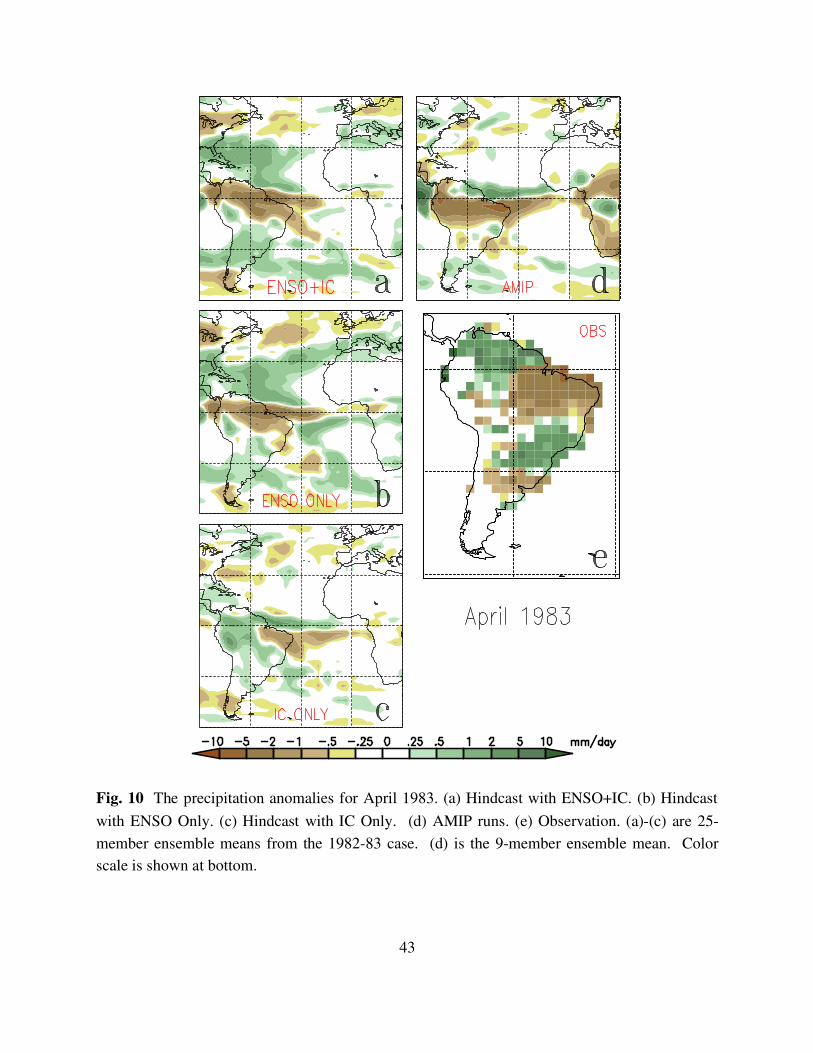
Fig. 10 The precipitation anomalies for April 1983. (a) Hindcast with ENSO+IC. (b) Hindcast

with ENSO Only. (c) Hindcast with IC Only. (d) AMIP runs. (e) Observation. (a)-(c) are 25-

member ensemble means from the 1982-83 case. (d) is the 9-member ensemble mean. Color

scale is shown at bottom.

43

Fig. 11 Same as Fig. 10 but for April 1996 (hindcast runs for the 1995-96 case). (a) ENSO+IC.

(b) ENSO Only. (c) IC Only. (d) AMIP runs. (e) Observation.

44

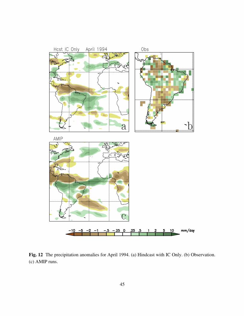
Fig. 12 The precipitation anomalies for April 1994. (a) Hindcast with IC Only. (b) Observation.

(c) AMIP runs.

45

Fig. 13 Same as Fig. 12 but for April 1989 (hindcast runs for the 1988-89 case). In panel (c), the

red boxes north and south of the equator over South America indicate the pNSA and pSSA

regions, respectively, used for Fig. 14.

46

Fig. 14 The root-mean-square error in the precipitation anomaly for April of year 1 averaged

over the pNSA (top panel) and pSSA (bottom panel) regions as defined in Fig. 13c. The error is

calculated from the r.m.s. of the ensemble mean of the hindcast minus observation at every grid

point over land within the box. The errors associated with the AMIP, ENSO+IC, ENSO-Only,

and IC-Only runs are shown in green, red, blue, and gray. The three groups of bars at left are for

the three individual post-1980 ENSO events discussed in the text. The group marked by "AVE"

is the average over the three events. The error for the neutral year 1994 is shown at right.

47

Fig. A1 The SST averaged over the South Atlantic box in Fig. 1c from observation (black, with

repeated seasonal cycle) and a 5-yr test run of the AGCM+ML model (red).

48

Fig. B1 (a) The model simulated response to the tropical Pacific ENSO forcing in the vertically

averaged temperature, defined as the mass-weighted average of temperature from the surface to

� � 0.1, where � is the terrain-following "sigma" coordinate. Shown is the temperature

anomaly averaged from January-May 1983. (b) The observational counterpart of (a), constructed

from sigma-level temperature data from NCEP reanalysis. Contour interval is 0.2°C. Red and

blue are positive and negative, respectively. Areas with the absolute value of the temperature

anomaly less than 0.2°C are not colored.

49