H I G H W A Y R E S E A R C H B O A R D

Bulletin 240

Highway Accident Studies

\s>mm OF

L I B R A R Y

IV1AY4 1960

'AL RESEARCH

National Academy of Sciences^

National Research Council pub l i ca t ion 7 2 6

HIGHWAY RESEARCH BOARD Officers and Members of the Executive Committee

1959

OFFICERS HARMER E . DAVIS, Chairman P Y K E JOHNSON, First Vice Chairman

W. A. BUGGE, Second Vice Chairman F R E D BURGGRAF, Director E L M E R M . WARD, Assistant Director

Executive Committee B E R T R A M D . T A L L A M Y , Federal Highway Administrator, Bureau of Public Roads (ex

officio) A . E . J O H N S O N , Executive Secretary, American Association of State Highway Officials

(ex officio) L O U I S JORDAN, Executive Secretary, Division of Engineering and Industrial Research,

National Research Council (ex officio) C. H . SCHOLER, Applied Mechanics Department, Kansas State College (ex officio. Past

Chairman 1958) R E X M . W H I T T O N , Chief Engineer, Missouri State Highway Department (ex officio.

Past Chairman 1957) R . R . B A R T L E S M E Y E R , Chief Highway Engineer, Ulinois Division of Highways J . E . B U C H A N A N , President, The Asphalt Institute W . A . BuGGE, Director of Highways, Washington State Highway Commission MASON A . B U T C H E R , Director of Public Works, Montgomery County, Md. C . D . C U R T I S S , Special Assistant to the Executive Vice President, American Road

Builders Association H A R M E R E . D A V I S , Director, Institute of Transportation and Traffic Engineering, Uni­

versity of California D U K E W . DUNBAR, Attorney General of Colorado

F R A N C I S V . DU PONT, Consulting Engineer, Cambridge, Md.

H . S . F A I R B A N K , Consultant, Baltimore, Md. P Y K E J O H N S O N , Consultant, Automotive Safety Foundation G . DONALD K E N N E D Y , President, Portland Cement Association B U R T O N W . M A R S H , Director, Traffic Engineering and Safety Department, American

Automobile Association G L E N N C . R I C H A R D S , Commissioner, Detroit Department of Public Works W I L B U R S . S M I T H , Wilbtir Smith and Associates, New Haven, Conn. K . B . WOODS, Head, School of Civil Engineering, and Director, Joint Highway Research

Project, Purdue University

Editorial Staff

F R E D BURGGRAF E L M E R M . WARD

2101 Constitution Avenue

HERBERT P . ORLAND

Washington 25, D . C.

The opinions and conclusions expressed in this publication are those of the authors and not necessarily those of the Highway Research Board.

VR^HIGHWAY R E S E A R C H BOARD Bulletin 240

Highway Accident Studies

Presented at the

38th ANNUAL MEETING

January 5-9, 1959

1960 Washington, D. C.

Department of Traffic and Operations

Donald S. Berry, Chairman Profejsor of Civil Engineering, Northwestern University

COMMITTEE ON SHOULDERS AND MEDIANS Asriel Taragin, Chairman

Highway Engineer, Highway Transport Research Branch, Bureau of Public Roads John L. Beaton, Supervising Highway Engineer, Materials and Research Department,

California Division of Highways W. R. B'iUis, Chief, Traffic Design and Research Section, Bureau of Planning and

Traffic, New Jersey State Highway Department Daniel Belmont, Institute of Transportation and Traffic Engineering, University of

California, Berkeley Louis E. Bender, Chief, Traffic Engineering Division, The Port of New York Authority C.E. Billion, Principal Civil Engineer, Bureau of Highway Planning, New York State

Department of Public Works Leon Corder, Traffic Engineer, Missouri State Highway Department, Jefferson City George F. Hagenauer, District Research and Planning Engineer, Illinois Division of

Highways J. A. Head, Assistant Traffic Engineer, Oregon State Highway Commission Fred W. Hurd, Director, Yale Bureau of Highway Traffic, New Haven J. W. Hutchinson, Instructor, Department of Civil Engineering, University of Illinois Harry H. lurka, Senior Landscape Architect, New York Department of Public Works,

Babylon, Long Island, New York Karl Moskowitz, Assistant Traffic Engineer, California Division of Highways Charles Pinnell, Assistant Research Engineer, Highway and Traffic Engineering,

Texas Transportation Institute, Texas A and M College Edmund R. Ricker, Traffic Engineer, New Jersey Turnpike Authority, New Brunswick J. L. Wehmeyer, Engineer of Traffic and Safety, Wayne County Road Commission,

Detroit

IC O COMMITTEE ON HIGHWAY SAFETY RESEARCH J.H. Mathewson, Chairman

Institute of Transportation and Traffic Engineering University of California, Los Angeles

Earl Allgaier, Research Engineer, Traffic Engineering and Saifety Department, American Automobile Association, Washington, D. C.

John E. Baerwald, Associate'Professor of Traffic Engineering, University of Illinois J. Stannard Baker, Director of Research and Development, Ti:affic Institute, North­

western University Abram M. Barch, Department of Psychology and Highway Traffic Safety Center,

Michigan State University, East Lansing Siegfried M. Breuning, Civil Engineering Department, Michigtan State University Leon Brody, Director of Research, Center for Safety Education, New York University Basil R. Crelghton, Assistant Executive Director, American Association of Motor

Vehicle Administrators, Washington, D. C. i John J. Flaherty, Director, Research Division, National Safety Council, Chic :^ Bernard H. Fox, Accident Prevention Program, U. S. Public jHealth Service Charles J. Keese, Texas Transportation Institute, Texas A and M College John C. Kohl, Director, Transportation Institute, University jof Michigan, Ann Arbor C. F. McCormack, Deputy Chief Engineer, Highways Division, Automotive Safety

Foundation, Washii^on, D. C. J. P. Mills, Jr., Traffic and Planning Engineer, Virginia Department of Highways Karl Moskowitz, Assistant Traffic Engineer, California Divi^on of Highways Charles W. Prisk, Supervising Highway Transport Research Engineer, Highway

Transport Research Branch, Bureau of Public Roads | William F. Sherman, Manager, Engineer and Technical Depajrtment, Automobile

Manufacturers' Association, Detroit G. D. Sontheimer, Director of Safety, American Trucking Associations, Inc. Virtus W. Suhr, Accident Research Analyst, Bureau of Traffic, Illinois Division of

Highways i Clifford O. Swanson, Chief of Research and Statistics, Department of Public Safety,

State of Iowa S. S. Taylor, General Manager, Department of Traffic, City of Los Angeles Wayne N. Volk, Engineer of Traffic Services, State Highway Commission of Wisconsin J. L. Wehmeyer, Engineer, Traffic and Safety, Wayne County Road Commissioners,

Detroit ^ Wilbur M. White, Highway Safety Service, Hillsboro, Ohio John Whitelaw, Brig. Gen. USA (ret.), Librarian, Highway t r a f f i c Safety Center,

Michigan State University, East Lansing

COMMITTEE ON ROAD USER CHARACTERISTICS T. W. Forbes, Chairman

Highway Traffic Safety Center, Michigan State University Terrence M. Allen, Department of Psychology and Highway Traffic Safety Center,

Michigan State University, East Lansing Earl AUgaier, Research Engineer, Traffic Engineering and Safety Department,

American Automobile Association, Washington, D. C. Siegfried M. Breuning, Civil Engineering Department, Michigan State University Leon Brody, Director of Research, Center for Safety Education, New York University Harry W. Case, Department of Engineering, University of California, Los Angeles William G. Eliot, 3d, Highway Engineer, Bureau of Public Roads Bernard H. Fox, Accident Prevention Program, U. S. Public Health Service Gordon K. Gravelle, Deputy Commissioner, Department of Traffic, New York, N.Y. William Haddon, Jr., Director, Driver Research Center, New York State Department

of Health Fred W. Hurd, Director, Yale Bureau of Highway Traffic, New Haven Joseph Intorre, Administrative Assistant, Institute of Public Safety, Pennsylvania

State University Merwyn A. Kraft, Research Coordinator, Flight Safety Foundation, New York A. R. Lauer, Professor of Psychology, Driver Research Laboratory, Iowa State College David B. Learner,' Human Factors Research Group, Research Laboratories, General

Motors Corporation, Detroit James L. Malfetti, Executive Officer, Safety Education Project, Teachers College,

Columbia University Alfred L. Moseley, Moseley and Associates, Boston Charles W. Prisk, Director, Highway Safety Study, Bureau of Public Roads Robert V. Rainey, Driver Research Project, University of Colorado Medical Center David W. Schoppert, Automotive Safety Foundation, Washington, D. C. Virtus W. Suhr, Accident Research Analyst, Illinois Division of Highways Clifford O. Swanson, Chief, Research and Statistics, Iowa Department of Public Safety Julius E. Uhlaner, Research Manager, Personnel Research Branch, TAGO, Depart­

ment of the Army, Washington, D. C. George M. Webb, California Division of Highways

Contents STATISTICAL DETERMINATION OF E F F E C T OF PAVED SHOULDER

WIDTH ON T R A F F I C ACCIDENT FREQUENCY R. C. Blensly and J . A. Head 1

Appendix A: Source of Raw Data 10 Appendix B: IBM Procedures 13 Appendix C: Statistical Procedures 16

FACTOR ANALYSIS OF ROADWAY AND ACCIDENT DATA John Versace 24

Appendix: Correlations 30

ACCIDENT ANALYSIS OF AN URBAN EXPRESSWAY SYSTEM A. F . Malo and H. S. Mika 33

Appendix A 41 Appendix B 42

INTERCHANGE ACCIDENT EXPOSURE S. M, Breuning and A. J . Bone 44

INVENTORY SPEED RESPONSES AND PRIOR T R A F F I C RECORDS AS PREDICTORS OF SUBSEQUENT T R A F F I C RECORDS

Harry W. Case and Roger G. Stewart 53

Statistical Determination of Effect of Paved Shoulder Width on Traffic Accident Frequency R. C. BLENSLY, Planning Survey Engineer, and J. A. HEAD, Assistant Traffic Engineer, Oregon State Highway Department

This investigation represents research by the Oregon State Highway Department in the use of statistics to explain how the width of paved shoulders on level and tangent rural two-lane highways affects ac­cident frequency.

Two different approaches were taken. Correlation procedures were used to evaluate the relationship between paved shoulder width and ac­cident occurrence, and variance measures were employed to analyze the difference between the average accident frequency on sections with narrow paved shoulders (4 f t or less) and the average accident frequency on sections with wide paved shoulders (8 f t or more).

The partial correlation technique established that when the effects of other roadway elements were eliminated and the sections grouped in various ADT ranges, no significant relationship between accident frequency and paved shoulder width was evident except in the 2,000-2, 999 ADT range where property damage and total accidents showed a significant tendency to increase in frequency as paved shoulder width increased.

The analysis of co-variance procedure established that when the effect of ADT was controlled there was a significantly higher mean number of property damage and total accidents on sections with wide paved shoulders than there was on sections with narrow paved shoul­ders in the 1,000-5, 600 ADT range.

The results of this study should be interpreted with extreme caution, inasmuch as the traffic volumes on the bulk of the sections were less than 5,000 vehicles per day. For this reason, i t would be erroneous to generalize that in all cases the number of accidents wil l be higher on sections with wide paved shoulders than on those with narrow paved shoulders. On the other hand, i t cannot be shown that increasing the width of the paved shoulder is actually helpful in reducing the accident frequency on level and tangent rural two-lane highways with traffic volumes in the ranges studied.

• THE PRESENT investigation represents research by the Oregon State Highway De­partment in cooperation with the Highway Research Board Committee on Shoulders and Medians in the use of statistics to explain how the width of paved shoulders on level and tangent sections of rural two-lane highways affects the accident frequency. The purpose of the HRB committee is to examine the influence of shoulders on traffic operations. This committee has recently been expanded to include the study of medians.

The concept, in Oregon, of paving shoulders was f i rs t introduced in 1950. Although the shoulders on several miles of highways have been paved since that time, the total mileage of level and tangent rural two-lane highways with paved shoulders was stil l somewhat limited in 1957. Tn order to obtain a sufficient number of sample elements, each 1-mi section of rural two-lane highway which was level and tangent and had paved shoulders was multiplied by the number of fu l l years for which accident data were a-vailable after the paved shoulders were constructed. In this way, the 96 sections of highway meeting these criteria were expanded to 346 sample elements. Forty-eight of these 346 sample elements were found to be in the 0-999 ADT range; these were excluded from further analysis because they had no variation in shoulder width. This left 298 usable sample elements.

Two different approaches were taken in this research project. Correlation pro­cedures were used to evaluate the relationship between accident frequency and the width of paved shoulders. The results of this analysis were based on the 298 sample elements. Variance measures were employed to analyze the difference between the average accident frequency on sections with wide paved shoulders (8 f t or more) and the average accident frequency on sections with narrow paved shoulders (4 f t or less). The 33 sample elements with 5-, 6-, and 7-ft paved shoulders were excluded from this phase of the study, leaving a total of 265 sample elements for analysis. No at­tempt should be made to compare the results of these two analyses because of dif­ferences in base data and in objectives.

In this report the frequency of personal injury, property damage, and total acci­dents was related to the width of paved shoulders. Through use of the aforemen­tioned statistical techniques, field controls, and arrangement of data, the influence on accident occurrence of roadway elements other than shoulder width was controlled.

The background of the various studies and the relationship between shoulder width and accident frequency have been reviewed briefly in an earlier publication (1). This earlier study indicated that the relationship between shoulder width and accidents was somewhat ambiguous. For example, Raff (2̂ ) found no relationship between accident s and shoulder width taken alone. By contrast, Belmont (3) found a tendency for per­sonal injury accidents to increase with paved shoulder wiHth in the 2,000-12,000 ADT range.

The California study by Belmont dealt exclusively with personal injury accidents, whereas the present investigation extended the analyses to the property damage and total accident categories as well.

This study does not provide information with respect to the relationship between shoulder width and accident frequency for all types of highways. Rather, the findings herein are based on data taken from sections the bulk of which had traffic volumes of less than 5,000 vehicles per day. The study was confined to rural two-lane sec­tions that were essentially straight and level.

DATA SOURCES Field Data

The field data were obtained on state primary rural two-lane highwa>d with paved shoulders. In addition to the width of the paved shoulders, the field observers re­corded the measurements of the following roadway elements:

1. Lane width 2. Sight distance restriction 3. Description of terrain

A detailed description of the field procedures, along with a sample field sheet, appears in Appendix A.

This information was necessary in order to determine which sample elements met the criteria of the study. For example, the lane widths were recorded in order to an­alyze the effects that might be associated with the paved lane width as contrasted with the paved shoulder width. Also, no sections were included which had a lane width less than 10 f t .

Only those 1-mi sections which had 30 percent or less sight restriction were in­cluded in this investigation. To meet this criterion a section could have at most only one portion wherein sight distance was less than 1, 500 f t . This virtually eliminated the sections with rolling or mountainous terrain.

Of the 366 mi of highway surveyed, there were 96 one-mi sections of level and tan­gent rural two-lane highway with paved shoulders, which as previously outlined af­forded 346 sample elements.

Accident Data The accident data used in this study were available in the Accident Analysis Section

of the Traffic Engineering Division, Oregon State Highway Department. Accidents

were tabulated for each fu l l year after paved shoulder construction was completed, and were classified as personal injury, property damage, and total accidents.

Traffic Volume Data The ADT values for the appropriate years for each one-mi section were taken from

Traffic Volume Tables compiled by the Oregon State Highway Department. An ADT value was assigned to each section for each year that i t was included in the study.

ANALYSIS Table 1 shows the distribution of the sample elements by shoulder width, lane

width, and ADT range. Examination of this table reveals that there is no uniform dis­tribution of sample elements. Only 10 percent were in the 5-, 6-, and 7-ft shoulder width category. Sixty percent were in the narrow shoulder category and the remaining 30 percent were in the wide shoulder category.

Of the sample elements in the narrow shoulder category, 23 percent were in the 0-999 ADT range. The wide shoulder grouping had no sample elements in this ADT range. Eleven percent of the narrow shoulder samples were in the 3,000-5, 600 ADT range, whereas 36 percent of the wide shoulder group fel l in this ADT range.

Lane widths for 63 percent in the narrow shoulder category were less than 12 f t . Only 31 percent of the wide shoulder sections had less than 12-ft lane width.

Examination of Table 1 further reveals that when the 0-999 ADT range was elimi­nated from further consideration, the vast majority of the sample elements were sec­tions with volumes of less than 3,000 vehicles per day. Traffic volumes on the bulk of 67 sample elements in the 3,000-5, 600 ADT range were less than 5,000 vehicles per day.

Jn view of this non-uniform distribution and the fact that prior research (4) estab­lished that accident occurrence increases with increased traffic volumes, i t was necessary to control the effects of lane width and ADT in order to establish the true relationship between accident frequency and shoulder width. These roadway elements were controlled, as mentioned, through the use of statistical techniques and field con­trols, and by grouping the sample elements into various ADT ranges as shown in Table 1.

The distribution of sample elements by number of accidents within the various shoulder width and ADT groups appears in Table 2, which shows frequency, f, and percent of the sample elements having given numbers of accidents, A. The product of the number of accidents. A, and the f r e ­quency of sample elements, f, having A acc idents is the total number of accl -dents, fA. Thus, in the 3- to 4-ft shoul­der width group (ADT 1, 000-1,999), 13 sample elements, or 37 percent, had no accidents. In the 5- to 7-ft shoulder width group (ADT 3,000-5, 600) one of the six elements had zero accidents, three had one, one had three, and one had four, making a total of 10 accidents.

A comparison of the total number of accidents and sample elements reveals that the ratio of the number of accidents to the number of sample elements in­creased as the shoulder width increased within a given ADT range: i . e., 39/35 << 45/^7 < 93/46 in the 1,000-1, 999 ADT range; 121/102 < 52/21 in the 2,000-2, 999 ADT range. In the 3,000-5, 600 ADT range, there was a slight inversion in this trend, but the highest prevailing ratio was stil l in the wide shoulder group.

TABLE 1 DISTRraUTION OF SAMPLE ELEMENTS

BY SHOULDER WIDTH, LANE WIDTH, AND ADT RANGE

ADT Ranee Shoulder Shoulder Lane No. of Width Width Elements 0-999* 1,000- 2,000- 3,000-

(ft) (ft) 1,999 2, 999 5,600

10 16 2 5 9 Q 11 115 30 22 61 2

3-4 12 65 14 8 26 17 13 12 _2 _0 _6 _4

208 48 35 102 23 10 3 0 3 0 0 11 30 0 24 0 6

5-7 12 0 0 0 0 0 13 0 0 0 0 0

33 0 27 0 6 10 0 0 0 0 0 11 33 0 24 9 0

St 12 46 0 10 8 28 13 26 0 12 4 10

105 0 46 21 38 Total 346 48 108 123 87 *Not included in analyses because shoulder width was 4 f t for aU.

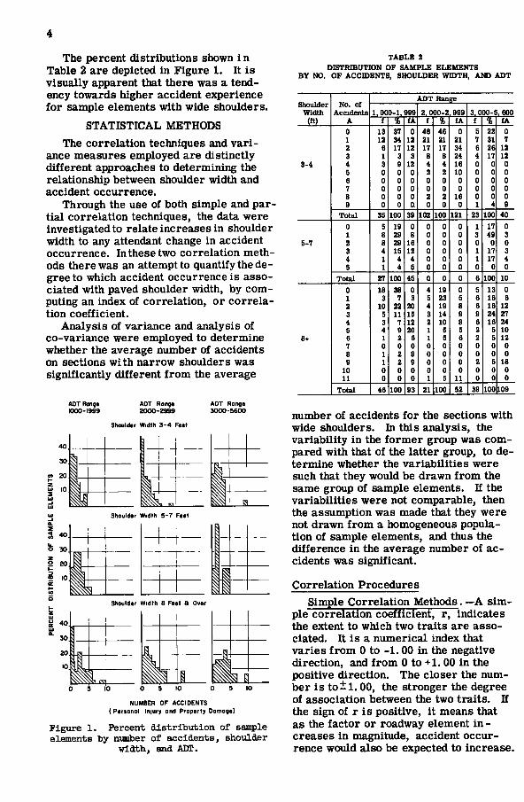
The percent distributions shown i n Table 2 are depicted in Figure 1. It is visually apparent that there was a tend­ency towards higher accident experience for sample elements with wide shoulders.

STATISTICAL METHODS The correlation techniques and vari­

ance measures employed are distinctly different approaches to determining the relationship between shoulder width and accident occurrence.

Through the use of both simple and par­tial correlation techniques, the data were investigated to relate increases in shoulder width to any attendant change in accident occurrence. In these two correlation meth­ods there was an attempt to quantify the de­gree to which accident occurrence is asso­ciated with paved shoulder width, by com­puting an index of correlation, or correla­tion coefficient.

Analysis of variance and analysis of co-variance were employed to determine whether the average number of accidents on sections with narrow shoulders was significantly different from the average

T A B L E 2 DISTRIBUTION OF S A M P L E ELEMENTS

B Y NO. OF ACCIDENTS, SHOULDER W I D T H , A N D A D T

ADTRwige ADT Ranga 1000-1999 2000-2999

Shoulder Width 3-4 F<et

ADT Ronga 3000-5600

40

30

</> 20 t-z lit 10 2

10 UJ _ l u UJ -1 Q. Z < tn

40 u. o 30 z o 20 \~ 3 03 10, fE t-co O »-z u a: 40

a. 30

20

10

—

r — —

1 J.

1 Shoulder Width S-7 Feet

1 1 1 1 1

1

Shoulder Width B Feet a Over

1

1 1

1

1 1 1 1 NUMBER OF ACCIDENTS

{Personol Injury and Property Damage)

Figure 1. Percent distribution of sample elements by number of accidents, shoulder

width, and ADT.

Shoulder No. of ADT Range

Shoulder No. of Width Accidents 1.000-1.999 2,000-2.999 3.000-5. 600

(ft) A t % £A f % fA f % fA 0 13 37 0 48 46 0 5 22 0 1 12 34 12 21 21 21 7 31 7 2 6 17 12 17 17 34 6 26 12 3 1 3 3 8 8 24 4 17 12

3-4 4 3 9 12 4 4 16 0 0 0 5 0 0 0 2 2 10 0 0 0 6 0 0 0 0 0 0 0 0 0 7 0 0 0 0 0 0 0 0 0 8 0 0 0 2 2 16 0 0 0 9 0 0 a 0 0 0 1 4 9

Total 35 100 39 102 100 121 23 100 40

0 5 19 0 0 0 0 1 17 0 1 8 29 8 0 0 0 3 49 3

5-7 2 8 29 16 0 0 0 0 0 0 3 4 15 12 0 0 0 1 17 3 4 1 4 4 0 0 0 1 17 4 5 1 4 5 0 0 0 0 0 0

Total 27 100 45 0 0 0 6 100 10

0 18 38 0 4 19 0 5 13 0 1 3 7 3 5 23 5 6 16 6 2 10 22 20 4 19 8 6 16 12 3 5 11 15 3 14 9 9 24 27 4 3 7 12 2 10 8 6 16 24 S 4 9 20 1 5 5 2 5 10 6 1 2 6 1 5 6 2 5 12 7 0 0 0 0 0 0 0 0 0 8 1 2 8 0 0 0 0 0 0 9 1 2 9 0 0 0 2 5 18

10 0 0 0 0 0 0 0 0 0 11 0 0 0 1 5 11 0 0 0

Total 46 100 93 21 100 52 38 100 109

number of accidents for the sections with wide shoulders, hi this analysis, the variability in the former group was com­pared with that of the latter group, to de­termine whether the variabilities were such that they would be drawn from the same group of sample elements. If the variabilities were not comparable, then the assumption was made that they were not drawn from a homogeneous popula­tion of sample elements, and thus the difference in the average number of ac­cidents was significant.

Correlation Procedures Simple Correlation Methods. —A sim­

ple correlation coefficient, r, indicates the extent to which two traits are asso­ciated. It is a numerical index that varies from 0 to -1.00 in the negative direction, and from 0 to +1. 00 in the positive direction. The closer the num­ber is to± 1.00, the stronger the degree of association between the two traits. If the sign of r is positive, i t means that as the factor or roadway element in -creases in magnitude, accident occur­rence would also be expected to increase.

Where r has a negative value, i t means that as the roadway element increases in mag­nitude, accident occurrence should decrease. This simple correlation coefficient must be interpreted with caution. It definitely does not, by itself, reveal the extent to which one of the traits (shoulder width, for example) causes the other factor (accident occurrence). It merely indicates how much, as one of the factors varies in a given direction, the other factor varies also in the same or the opposite direction.

Another precaution in interpretation must be urged in regard to the magnitude of the correlation coefficient. It is possible for the correlation coefficient between two traits to be rather high and yet not be significant, because there is no indication wheth­er the relationship shown is chance or causal. Correlation coefficients which are not significant have no more value than a coefficient of zero.

Table 3 presents the correlation coefficients between accident frequency and the various roadway elements—shoulder width, ADT, sight restriction, lane width, p r i ­vate driveways, public driveways, number of intersections, intersectional access points, and total access points. It wi l l be noted that each of the roadway elements was correlated with personal injury, property damage, and total accidents in each of three ADT ranges.

Because all sections in the less than 1, 000 ADT rai^e had shoulders 4 f t or less in width, it was impossible to evaluate the relationship between shoulder width and acci­dent occurrence on these sections.

Table 3A discloses that there was a significantly reliable tendency for personal in­jury accidents to increase as shoulder width increased in the 2,000-2, 999 ADT range.

In Tables 3B and 3C, i t is seen that there was a significantly reliable tendency for property damage and total accidents to increase as shoulder width increased in all three ADT ranges.

Table 3C further reveals that with respect to total accidents, the relationship be­tween accidents and shoulder width was stronger than the relationship between acci­dent occurrence and any other roadway element. In addition to shoulder width, only ADT, lane width, and sight restriction exhibited indications of being significantly re­lated to accident occurrence.

In general, property damage accidents were more strongly related to roadway ele­ments than were personal injury accidents.

The interpretation of the foregoing results may be facilitated by asking two very distinct questions:

1. Was there a tendency for the accident frequency to increase with increases in the shoulder width?

2. If so, was the increase in shoulder width responsible for the increase in acci­dent frequency?

The answer to the f i rs t of these questions is in the affirmative, expecially for prop­erty damage and total accidents. This relationship also prevails in the 2,000-2, 999 ADT range for personal injury accidents.

TABLE 3 SUMMARY OF SIMPLE COHRELATION COEFFICIENTS BETWEEN ROADWAY ELEMENTS AND ACCIDENT OCCURRENCE

3A - Correlations With Personal Injury Accidents ADT Range Shoulder ADT

Sight Restriction

Lane Width

Private Driveways

Public Driveways

Inter­sections

Intersectional Access Points

Total Access Points

1,000-1,999 2,000-2,999 3,000-5, 600

.189

.204*

.068

.271 -.106 .133

.006 -.130 -.243

.223*

.086

.129

.075

.013

.025

-.007 .112 .143

.094 -.016 -.048

.037

.031 -.022

.059

.050

.089 3B - Correlations With Proi lerty Damage Accidents

1,000-1,999 2,000-2,999 3,000-5, 600

.319°

.24?

.275''

.366° -.061

.362°

-.021 -.129 -.234

.273*

.015

.203

.126

.054 -.103

-.019 .131 .047

.140

.069 -.030

.066

.044

.012

.097

.088 -.037

3C - Correlations With Total Accidents 1,000-1,999 2,000-2,999 3,000-5, 600 5* ^ 1

.330°

.268°

.257'

.397"' -.089^ .358°

-.016 -.152 -.302*

.303''

.046

.255

.131

.047 -.073

-.018 .147 .103

.149

.048 -.046

.068

.047

.000

.101

.088

.011 Significant at the 5 percent level of confidence: One Ume in 20, coefficient may result from chance. Significant at the 1 percent level of confidence: One time m 100, coefficient may result from chance.

6

With regard to the second question, the answer must for the moment remain indefi­nite. It is not possible to ascertain on the basis of simple correlation methods whether the increases in accident frequency were caused by increases in shoulder width.

Partial Correlation Methods. —The partial correlation methods differ considerably from simple correlation techniques, in that they provide for inferences about the nature of the cause of a given relationship. In a partial correlation coefficient, such as that between accident occurrence and shoulder width, the effects of other factors have been controlled (eliminated) by this statistical procedure. The quantitative interpretation of partial correlation coefficients is the same as that for simple correlation coeffi­cients. The individual partial correlations are shown in Table 4.

Table 4 contains the same groupings that appeared in Table 3. The correlations shown in Table 4 are indexes of the pure relationship between two traits without the interfering effects of other factors. If a correlation coefficient in Table 3 was signifi­cant, i t meant only that there was a significant degree of association between accident frequency and the roadway element in question. However, i t could not be established whether the roadway element was responsible for the increase in accident occurrence. By contrast, if there is significant relationship between accident frequency and a road­way element in Table 4, i t may be assumed that there was a true causal relationship between the roadway element and accident occurrence. Just as the correlation coeffi­cients in the shoulder width column indicate the relationship between shoulder width and accident occurrence, with the effects of all of the other roadway elements elimi­nated, so the correlation coefficients in any other column indicate the true relationship between that single roadway element and accident occurrence with the effects of all the other roadway elements, including shoulder width, controlled.

Table 4 shows that the frequency of property damage and total accidents was signifi­cantly related to shoulder width only in the 2,000-2,999 ADT range. Personal injury accidents show no relationship to shoulder width. Thus, when the influence of other roadway elements was controlled, those significant relationships between accident frequency and shoulder width determined by the simple correlation technique tended to disappear. This indicates that the relationships which disappeared were only coinci­dental.

It is also noted that total accidents were related to ADT on higher volume sections. Except for this relation and the association with shoulder width, accident occurrence was not related to any other roadway element when the influence of other roadway ele­ments was controlled.

It is evident from the foregoing that a real relationship between accidents and shoul­der width does not exist in all ADT ranges. It would be fair to conclude, however, that when the influence of ADT and other roadway elements is controlled, property damage and total accidents increase in number as the width of paved shoulders increases on highways in the 2,000-2,999 ADT range. Consequently, i t may be stated that the in ­crease in paved shoulder width is responsible for the increase in accident frequency in the 2, 000-2, 999 ADT range.

TABLE 4 SUMMARY OF PARTIAL CORRELATION COEFFICIENTS BETWEEN ROADWAY ELEMENTS AND ACCIDENT OCCURRENCE

4A - CorreUtlong With Peraoial Inlury Accidents ADT Range Shoulder ADT

Sight Restriction

Lane Width

Private DrlTeways

PubUc Driveways

Inter­sections

Ihtersectional Access Points

Total Access Points

1,000-1,999 2,000-2,999 3,000-5, eoo

.037

.171 -.155

.272" -.034 .185

.077 -.020 -.251

.204

.106

.075

-.002 -.110 -.082

-.002 -.081 -.078

.040 -.072 -.157

-.002 -.068 .029

-.002 .105 .102

4B - Correlations With Property Damage Accidents

1,000-1,999*' 2,000-2,999 3,000-5, eoo

.081-

.239 -.040

.003

.340" -.159 -.160

-.060 .128

.076 -.010

.096 -.019

.117 -.207

.056

.164 .076 .024

- 4C - CorrelatianB mth Total Accidents 1,000-1,999° 2,000-2,999 3.000-5,600

.059

.253* -.112

.059

.380* -.135 -.260

-.004 .146

.015 -.050

.043 -.055

.063 -.253

.017

.155 -.017 .072

" Significant at the 5 percent level of confidence: One time In 20, coefficient may result from chance. Coefficients computed for one element only.

Variance Procedures Analysis of Variance. —In the simple and partial correlation procedures previously

described, an attempt was made to determine whether there was a trend in accidents with a successive increase in shoulder width. Paved shoulder widths on the sections studied ranged from a minimum of 3 f t to a maximum of 10 f t .

Variance procedures are designed to contrast the frequency of accident occurrence on the sections with narrow shoulders with the frequency of accident occurrence on those sections having wide shoulders. A description of these statistical techniques wil l be found in Appendix C.

It is not possible to control the influence of other roadway elements in the analysis of variance procedure. In that i t is only possible to establish whether or not a tend­ency is apparent, i t is similar to the simple correlation technique.

The f i rs t step in analysis was to group the data by accident classification (personal injury, property damage, and total accidents). Within these major groups, subgroups were made for shoulder width and ADT range. These groupings are shown in Table 5.

Column 1 of Table 5 contains the sources of variation — shoulder width, ADT range, interaction of shoulder width and ADT range, and residual error. This last is a factor which results when these three major factors are removed from the data. (See Ap­pendix C.)

Column 2 shows the mean number of accidents in each shoulder width category and each ADT range. The differences in these means wil l be tested by variance proce­dures for significance.

Column 3 indicates the corresponding degrees of freedom (described in Appendix C). Columns 4 and 5 show the error estimate (variance estimate) and F ratio, respec­

tively. (See Appendix C.) The F ratio indicates whether or not the sample means were

TABLE 5 ANALYSIS OF ACCIDENT FREQUENCY BY SBOULDER WIDTH AND ADT RANGE

5A - Personal Injury Accidents Source of Variation

(1)

Mean Number of Accidents

(2)

Degrees of Freedom

(3)

Error Estimate

(4)

F RaUo (5)

InterpretaUon (8)

Shoulder width: 4 f t or less 8 f t or more

0.36) 0.61 f 1 1.42 2.54 Variance in shoulder width resulted in no difference in

personal injury accident frequency. ADT range:

1,000-1,999 2,000-2,999 3,000-5,600

0.33) 0.41 y 0.74)

2 2.66 4.75a There was a significantly higher number of personal injury accidents on high ADT sections.

Interaction Error : 2

259 0.26 0.56

-SB - Property Damage Accidents

Shoulder widtli: 4 f t or less 8 f t or more

0.89 I 1.81) 1 38.52 16. 53* There was a significanUy higher number of property

damage accidents on sections with wide shoulders. ADT range:

1,000-1,999 2,000-2,999 3,000-5,800

1.30) 1.00> 1.70)

2 2.55 1.09 Van ance in ADT resulted in no difference in property damage accident frequency.

Interaction Error

- 2 259

0.34 2. 33

-

Shoulder width: 4 f t or less 8 f t or more

1.2s) 2.42) 1 62.26

ADT range: 1,000-1,999 2,000-2,999 3,000-5,600

1.63) 1 . 4 l | 2.44)

2 10.10

Interaction Error IL a i — i . . > * ^ 1 1 -

2 259

0.68 3.58

5C - Total Accidents

17. 39a

2.82

There was a significanUy higher number of total acci­dents on sections with wide shoulders.

Variance in ADT resulted in no difference in total acci­dent frequency.

confidence: in 100, F ratio may result from chance.

8

significantly different from each other, and were used as a criterion in making the in­terpretation (Column 6).

Examination of Table 5A discloses that personal injury accident frequency on sec­tions with narrow shoulders was not significantly different from the personal injury accident frequency on sections with wide shoulders. It is seen, however, that the ac­cident frequencies in different ADT ranges were significantly different from each other. This fact pointed up the strong influence ADT had on accident frequency.

Table 5B indicates that there was a significantly higher number of property damage accidents on sections with wide shoulders than there was on sections with narrow shoul­ders without consideration of the influence of ADT. In this accident category, ADT did not appear to have much influence on the accident frequency.

The results shown in Table 5C for total accidents were the same as shown in Table 5B. Because the bulk of the total accidents was composed of property damage acci­dents, i t was expected that the results for these two accident classes would be similar.

Again, the interpretation of these findings may be facilitated by asking two questions: 1. Was there a tendency for sections with wide shoulders to have a higher mean num­

ber of accidents? 2. K so, were the wide shoulders responsible for the higher mean number of acci­

dents? The answer to the f i rs t question is in the affirmative with respect to property dam-

age and total accidents. Although a similar trend emerged in the personal injury ac­cident category, i t was not statisticaUy reliable.

With regard to the second question, i t is not possible to ascertain on the basis of analysis of variance measures whether the width of the paved shoulder caused the higher accident experience. This question can, however, be answered through use of the an­alysis of co-variance procedure.

Analysis of Co-Variance. —The co-variance procedure is similar to the partial cor-relation technique discussed previously because the effect of a second factor can be e-liminated so that the true effect of the factor in question can be evaluated.

It wi l l be recalled that the partial correlation technique disclosed that ADT was the only factor other than the shoulder width that was significantly related to accident oc­currence. In the analysis of variance, ADT also emerged as a contributing factor to accident occurrence. In recognition of the stroi^ influence ADT seemed to have on ac­cident occurrence, i t was decided to control i t in this analysis so that the difference in accident frequency between sections with narrow shoulders and sections with wide shoulders could be tested for significance.

In this analysis, the data were again grouped according to accident classification, and the only source of variation was shoulder width as shown in Table 6. As in the previous analysis, the F ratio indicates the degree of significance of the difference in accident frequency between sections with narrow shoulders and sections with wide shoulders.

TABLE 6 ANALYSIS OF EFFECT OF SHOULDER WIDTH ON ACCIDENT FREQUENCY WITH THE EFFECT OF ADT CONTROLLED

6A - Personal Ih]ury Accidents Source of Variation

Degrees of Freedom

Error Estimate

F Ratio Interpretation

Shoulder width 1 2.05 3.73

Width of slioulder made no difference m personal injury accident frequency.

Error 262 0.55 —

6B - Property D unage Accidents Shoulder

width 1 41.03 18.07* There was a significanUy higher number of property damage ac­cidents on sections with wide shoulders.

Error 262 2.27 -6C - Total Accidents

aioulder width

Error 1

262 61.51 3.49

> Slgnlilcant at tbe 1 percent level of confidence: One time in lo6, F ratio may result from chance.

17.62* There was a significantty higher number of total accidents on sections with wide stnulders.

9

Table 6A shows that the difference between the mean number of personal injury ac­cidents on sections with narrow shoulders and the mean number of personal injury ac­cidents on sections with wide shoulders was not significant when the effect of ADT was eliminated.

Tables 6B and 6C disclose tliat the difference between the mean number of property damage and total accidents on sections with narrow shoulders and sections with wide shoulders was significant when the effect of ADT was eliminated.

The results of this analysis lead to the conclusion that there were a significantly higher number of property damage and total accidents on sections with wide paved shoulders than there were on sections with narrow paved shoulders when the effect of ADT was controlled. Consequently, i t may be stated that the width of the paved shoul­ders was responsible for the higher number of accidents.

Summary of Analysis Two different approaches were taken in analyzing these data—namely, correlation

procedures and variance measures. Correlation procedures were used to evaluate the relationship between accident frequency and the width of paved shoulders. Vari­ance measures were used to analyze the difference between the average accident f re ­quency on sections with wide paved shoulders and the average accident frequency on sections with narrow paved shoulders.

Through the use of simple correlation procedures, i t was found that there was a statistically reliable tendency toward an increase in accident frequency as paved shoul­der width increased, especially in the property damage and total accident categories in all ADT raises investigated.

Through the use of partial correlation techniques, i t was established that when the effects of other roadway elements were eliminated, and the study sections grouped in various ADT ranges, no significant relationship between accident frequency and paved shoulder width emerged except in the 2,000-2,999 ADT range. In that area, property damage and total accidents showed a significant tendency to increase in frequency as paved shoulder width increased. No relationship appeared between frequency of per­sonal injury accidents and width of paved shoulders in the 1,000-5, 600 ADT range.

Through the use of the analysis of variance procedure, i t was found that without con­trol over the effect of ADT there was a statistically reliable tendency for sections with wide shoulders to have a higher mean number of property damage and total acci­dents than sections with narrow paved shoulders. Although a similar trend emerged in the personal injury category, i t was not statistically reliable.

Through use of the analysis of co-variance procedure, i t was found that when the ef­fect of ADT was controlled, there was a significantly higher mean number of property damage and total accidents on sections with wide paved shoulders than there was on sections with narrow paved shoulders in the 1,000-5, 600 ADT range.

On the basis of these findings, it would appear that construction of narrow paved shoulders on level and tangent rural two-lane highway sections with traffic of fewer than 5, 000 vehicles per day would contribute more to the safety of the motoring public than would the construction of wide paved shoulders.

Because these findings are contrary to a common belief that wide shoulders increase the safety of the highway, additional study and research should be made to establish be­yond any question of doubt the relationship between the number of accidents and the width of paved shoulders. Also desirable is information for sections of highway where traffic volume and geometric characteristics differ from those included in this study.

Discussion of Results There is a remote possibility that the higher mean number of accidents on sections

with wide paved shoulders resulted from the influence of some roadway elements other than shoulder width; this is unlikely, however, in view of the fact that the correlation techniques showed that no roadway elements other than shoulder width and ADT were related to accident frequency.

10

In an effort to explain this startling finding, i t was theorized that the reason for the greater hazard on sections with wide paved shoulders might be a narrower over-all (paved plus gravel) shoulder width. Examination of the sections within the 2, 000-2, 999 ADT range (the only AOT rai^e where the accident frequency increase with paved shoulder width increase was significant) disclosed that, in the main, the sections with wide paved shoulders had wider over-all shoulder widths than the sections with narrow paved shoulders.

It is interestii^ to note that Belmont (3) found a similar relationship between person­al injury accident frequency and paved shoulder width on sections rangii^ in volume from 2,000 to 12, 000 vehicles per day. Belmont concluded that "apparently the advan­tages of wider shoulders are more than offset by a tendency of drivers to be less care­ful . As shoulder width increases drivers may gain an unjustified feeling of security." This theory is one possible explanation for the relationship found in this study.

ACKNOWLEDGMENT Statistical Control by Noel F. Kaestner, Statistician, Oregon State Highway Depart­

ment; Professor of Psychology, Willamette University.

REFERENCES 1. Head, J. A . , and Kaestner, N. F . , "The Relationship between Accident Data and

the Width of Gravel Shoulders in Oregon." HRB Proc., Vol. 35, pp. 558-576 (1956).

2. Raff, Morton S., "Interstate Highways Accident Study. " Traffic Accident Studies, HRB Bulletin 74, pp. 18-45 (1953).

3. Belmont, D. M . , "Accidents versus the Width of Paved Shoulders on California Two-Lane Tangents-1951-1952." HRB Bulletin 117, pp. 1-16 (1956).

4. Schoppert, D. W., and Kaestner, N. F . , "Predictii^ Traffic Accidents from Road­way Elements —Rural Two-Lane Highways with Gravel Shoulders." HRB Bul­letin 158, pp. 4-26 (1957).

5. Cohen, Arthur, "Multiple Regression Analysis." IBM 650 Library, File No. 6.0.001.

6. Snedecor, G. W., "Statistical Methods." The Iowa State College Press, Ames, Iowa (1950).

Appendix A SOURCE OF RAW DATA

The raw data employed in this investigation were derived from two major sources. The f i rs t source was an observer working in the field. The second source was avail­able in the office.

Field Data The observer's task was to record shoulder and lane widths, percent sight restric­

tion, terrain description (level, rolling, or mountainous), and other pertinent remarks for each 1-mi section aloi^ the prescribed route. The car used was specially equipped with an odometer which permitted identification of the exact location at which measure­ments and other observations were made. Previously, field sheets had been prepared which provided ample space for the convenient recording of all data. A sample field sheet appears in Figure 2. The upper value in Column 2, "Pavement Width, " is the distance from the center stripe to the outer edge of the pavement, including the paved shoulder. The number below in parentheses is the paved shoulder width. The number in Column 3, "Gravel Shoulder Width, " is simply the width of the adjoining gravel shoulder beyond the edge of the paved shoulder.

At the beginning of each 1-mi section, the field observer would record the terrain description. The abbreviations L for level, R for rolling, and M for mountainous

11

Highway Ho. 6

0RS3QN SXAIB HIGHWAY DEPARTMENT Tra f f i c Bngineerlng Division

Planning S u r v ^ Section

PAVED SHOnUKR STUDT (Field Sheet)

EH

Roadway Characteristics

Width Measurement

l i igp : lilts'

Sight Restriction

Location to the Nearest One-Tenth of a Mile

Other Conments

(1) (2) (3) (4) (5) (6) (7)

L

®

3

2

®

6.0

6,Si B£-H e s

M.P. TIT

L

R

®

R

®

it. 14 (4) ®

Z

®

7.IB

r.6s z s

M R e . t r

14 (4)

3-

3

Z

®

B 55

M.P 9.17

/?

®

Z

3

®

9.20

9.7/

B -H t M.P/O./T

2 0

Figure 2.

were employed throughout and appear in Column 1. At the same location in the field, the observer would also measure the pavement width from center stripe to outer edge and gravel shoulder width to the nearest foot and record the results, as shown in Col­umns 2 and 3, respectively. After making these measurements and recordings, the observer would proceed along the section taking note of the terrain.

Somewhere farther on, usually in the middle of the section, the driver again made shoulder and lane measurements and also recorded the abbreviated description of the terrain. In this manner, at least two measurements were taken of the lane and shoul­der width within each mile. The mile post location of the f i rs t and second, and any other points of measurement within the 1-mi section, were recorded to the nearest 1/100 ml, as shown in Column 4. Total pavement width-that is, both lanes and left

12

and right shoulders —were measured at each stop. The gravel width was taken as that area which was obviously safe or practical for shoulder use.

Before leaving any particular section, the driver used the above measurements to determine the most representative pavement width from centerline to outside edge, paved shoulder width, gravel shoulder width, and terrain for the section. These data appear in circles in Columns 1, 2, and 3 for each 1-mi section.

In addition to the above measurements and recordings, the driver kept a continuous record of the presence or absence of sight restriction. The 1/10 mi divisions appear­ing in Column 5 of the field sheet were used in recording these data. As the observer proceeded through a section, special notations were made concerning the location of the beginning and end of restricted sight distance (less than 1, 500 f t of pavement visible). When the observer approached a section with restricted sight distance, he watched the road behind him to find the ending point of restricted sight distance for ve­hicles traveling in the opposite direction. Upon reaching that point, its location was noted in Column 5 on the field sheet. The letter E was used to designate this point. The beginning of sight distance restriction, designated B, for the observer's direc­tion of travel was 1, 500 f t (0. 3 mi) behind the point designated by the letter E. As the observer proceeded through the section with restricted sight distance, a point was se­lected which appeared to offer the end of restricted sight distance for that direction of travel and an E was recorded (correct to the nearest 0.1 mi) in Column 5 on the field sheet. The beginning of sight restriction for vehicles traveling in the opposite direc­tion was 1, 500 f t ahead of the point designated by the letter E.

Upon the field observer's return to the office, all 0.1-mi sections in either direc­tion of travel that did not have the required 1, 500-ft sight distance were blanked out (as indicated by vertical lines in Column 5). In this manner, i t was possible to deter­mine in steps of 5 percent the amount of sight restriction present for each 1-mi sec­tion, and these determinations appear in Column 6.

The data on the field sheets were transcribed in the office onto code sheets (Fig. 3). The terrain description presented on the field sheet in terms of a single letter abbre­viation was transformed into a numerical code wherein level, rolling, and mountainous were designated by 0, 1, and 2, respectively. The other data appearing on the code sheet were obtained in the office.

OBEQON STATE HII3IWA; DEPA8THENT T r a f f i c Engineering D i v i s i o n

Planning Survey Sec t ion

PATB) SHOnU>ER SIDDI (Code Sheet)

i 1

Beg

inn

ing

B

ile

Pos

t

Ave

rage

D

aUy

Tra

ffic

! 13

lan

e W

idth

Shoulders DHs

ion

sJI

Inte

rsec

tlon

al

Acc

ess

Poin

ts

OOH

n -42

Accident Data

i 1

Beg

inn

ing

B

ile

Pos

t

Ave

rage

D

aUy

Tra

ffic

1 T

erra

in

Per

cen

t Si

gh

Res

tric

tion

lan

e W

idth

Pav

ed

Gra

vel

Com

bine

d

Pri

vate

ion

sJI

Inte

rsec

tlon

al

Acc

ess

Poin

ts

OOH

n -42

Non-Intei , I n t e r . T o t a l i 1

Beg

inn

ing

B

ile

Pos

t

Ave

rage

D

aUy

Tra

ffic

1 T

erra

in

Per

cen

t Si

gh

Res

tric

tion

lan

e W

idth

Pav

ed

Gra

vel

Com

bine

d

Pri

vate

\\ (J a c

I Inte

rsec

tlon

al

Acc

ess

Poin

ts

OOH

n -42

1 Per

son

al

Inju

ry

Pro

per

ty

Dam

age

Per

son

al

liij

ury

P

rop

erty

D

amag

e P

erso

nal

In

jury

P

rop

erly

D

amag

e

06 00&/7 033 0 / o 0^ OZ 06 00 0/ 0 00 Of 00 00 00 0/ 00 0/

007I7 03d 0 o z s /O 07. Ob 00 00 0 00 00 00 00 00 00 00 00

0& 008/7 OfO / a s s /O OZ Ob 0 / 0/ 1 OZ OS 00 01 0/ OZ o r OS

009/7 040 / ozo / o oa 03 07 0/ 00 / <?/ 03 00 00 00 0/ 00 0/

1

Figure 3.

13

Office Data An estimate of the AOT for each section was developed from the data in Traffic Vol­

ume Tables for the years 1950-1957. The years employed depended on the year of com­pletion of the paved shoulder for the particular section in question. No section which had a very large percent difference in ADT from one point to another in the course of the mile was included in the study. Accident data and driveway data were available in the Accident Analysis Section of the Traffic Engineering Division. This section pro­vided accident data for each 1-mi stretch in the sample.

The number of personal injury, property damage, and total accidents in terms of accidents per mile per year was placed on the code sheets mentioned above. These included intersectional as well as non-intersectional accidents. The completed code sheet provided the following information for each 1-mi section: terrain, lane width, paved shoulder width, gravel shoulder width, percent sight restriction, ADT, personal injury, property damage, and total accidents for each year included in the study.

Appendix B IBM PROCEDURES

The data from the completed code sheets were punched onto IBM cards in a form dictated by the 650 prc^ram for partial and multiple correlation (5). This 650 sched­ule allowed only five variables to be dealt with on the f i rs t card for each sample sec­tion. In order to evaluate all the independent variables—i. e., roadway elements— a second card accompanied each of the original code sheet entry cards. From this point, the code sheets were no longer used directly but were retained as a duplicate record.

The f i rs t stage of the 650 program was to produce the simple intercorrelations be­tween the various roadway elements and all accident combinations. The results of this f i rs t 650 run were then fed back into the 650 for the second run. The by-products of the second run of the 650 were the partial correlation coefficients between the vari­ous roadway elements and accidents and the beta coefficients. These coefficients can be converted to "b" coefficients in the event multiple correlations are desired in the future. For purposes of this study, the partial correlations were the desired end re­sult. The availability of a 650 computer permitted partialing out as many as eight variables from the relationship between shoulder width and accident occurrence and computation of a tenth order partial correlation coefficient. A typical run for a given ADT group and accident class took approximately 20 minutes. It is estimated that i t would require at least one month of intensive work to compute a tenth order partial correlation on a desk calculator. In addition to this obvious saving in time, the 650 procedure provided the partial correlation between any two variables with all the rest controlled. In this way, the relationships between the roadway elements themselves could be evaluated independently of the other effects as well as the relationship between any single roadway feature and accident occurrence. Again, to compute the partial correlation on a desk calculator between any of these pairs of roadway elements with the others controlled would take approximately one month.

A pair of sample IBM cards appears in Figures 4 and 5. The type of information appearing there from left to right in columns so used, shown in parentheses, is as follows for Card 1 (Fig. 4): last digit of highway number (6), f i rs t three digits of the beginning milepost (7-9), accident frequency (12-13), ADT (22-23), percent sight re­striction (32-33), paved lane width (42-43), paved shoulder width (52-53), private driveways (62-63), public driveways (72-73).

On Card 2 (Fig. 5): intersections (12-13), intersectional access points (22-23), total access points (32-33).

14

cs> s OJ cn i n CO C/3 cn 3 r s i C O m CO l ~ " oc an s «M CO >«»• in CO r ~ eo cn n

S A V M 3 A m a G 3 C CM

CM CO CO

in i n

to CO

r~. eo e s

cn c en s

o n a n d CM CN

C O C O -* i n

m CO CO

p~ r »

eo C O

ar> c cn 7

CM CO i n CO r ~ to o> es c CM C O m CO es en s o CM C O m C O ^ oo 0 > es a CM C O i n l O oo en a ca 8 CM C O i n C O i ~ . eo cn s es s CM C O >* i n CO r ~ eo c n 8

S A V M S A l U a es s C3 8

CM CM

C O C O

m i n

CO CO

r » r—

eo eo

cn s es S

S l V A I d d <=> s <=> S

CM CM

C O CO

i n i n

CO tt>

i~» r »

eo oo

a> 8 en 3

S I 3 CM C O i n to i-» eo OS 8 c=> a CM C O i n CO oo at s

CM C O i n CO ^ eo at 5 » 8 CM C O i n CO ee en a o S CM C O i n cs eo e> s e S CM CO i n CO «o a> a

H i a i M CM C O m CO r» eo at s d S o m o H S

a a c a A

CM CM

C O C O

i n i n

CO CO

1 ^ r ~

eo eo at a

at a Q B A V d e> s CM CO i n CO i»- eo at s

ea s CM C O i n CO r » eo at a o X CM C O i n CO i ~ eo at 8 e» s CM C O i n CO r ~ eo

CM C O i n CO i«- eo at a o « CM C O m CO 1** eo at 9 es « CM C O i n CO r ~ eo 0 > 9

H i a i M CM C O m CO r«. eo at e

Q B A V d

a 9 CM C O i n CO r ~ ee c»« Q B A V d es s

CM CM

CO C O

m in

CO CO

eo ee

at 9 et> s es 3 CM CO «•• i n CO r » ee 0 > 9

e a *— CM C O x r i n CO ee at ft *— CM C O ««• i n CO p» ee at s

a 8 CM C O •« i n CO r » eo cn 9 S 8 CM C O i n CO r » eo at 8

N 0 l i 3 I H l S 3 1 ^ ^ CM CM

C O C O

i n i n

CO CO p~

ee ee

en 8 at s

1 H 9 I S c 9 CM C O i n c a r ~ eo at 8 1 N 3 D s s CM C O i n C O r » GO en a

U 3 d es s CM C O i n CO p~ eo at a

U 3 d s a CM C O X T i n CO r ~ eo en a e> n CM C O i n CO f~" ee en St a n CM C O i n C O i~» oo at s

CM CO i n CO p~ oo 0 5 S a R CM C O i n CO r-~ eo at St es CM C O i n CO r ~ oo at 8

CM C O i n CO r ~ eo er> es 8 CM C O i n CO p*» oo en 8 e> « CM C O i n CO r ~ oo at 8

CM C O i n CO eo en s CM C O i n CO eo o> a

es 8 CM C O x c i n CO r*» CO cn S CM C O m CO CO at c

es 8 CM C O i n CO r ~ . oo Ol s o s CM C O i n CO eo at s es ~ CM C O i n C O r-> ee cn s

v i v a CM C O x f i n «o i ~ - eo cn £

v i v a ^S " CM C O «* i n CO r ~ eo at s l N 3 a i 3 3 V CM

CM C O C O

x f i n i n

CO C O

r « p^

eo eo at :2

cn : , CM C O m CO r ~ . eo en s • CM C O i n CO ir~ cc> en s

e a := CM C O t o C O r - CO at ^ •ON a u v 3 . — CM C O m C O i ~ " vu at s

' d ' N - 9 3 8

, — CM C O x f i n ca < ^ tji •> ' d ' N - 9 3 8

. — CM CO m C O t~" cu (.•> ' d ' N - 9 3 8 CM C O m C O r « . aa •.Tt -

•ON ' A M H G 3 - CM C O i n C£> i ~ " eu «J> -. — CM C O i n CO t « - oo Hi •»

•ON o CM C O i n (S r~ ce <JV — •ON CM CO i n CO r ~ ee t » a o r CM CO m CO r» oo at »-

C9 - — CM C O •* i n r » oo en •

I

n

o

I

1

1

15

es s CM C O m iO r» C O o s CM C O m t o r~ CO en s e> s CM C O in C D i*» c» cn IE e> CM C O to CO r*. eo en

CM C O •n C O r—• C O o> s CM C O tn C O r~" eo c n s

C3 S CM C O in C O eo es s CM C O >n CO p» eo e » s CM C O •n CO eo en s o ;= CM C O in CO ^ eo cn o s CM C O m CO C O C3 S B 8 CM C O in CO r— cse en s ei s CM C O in CO r~ eo cn s es s CM C O in CO r— eo ei s ea a CM C O in CO p~ eo C3 S CM C O in CO r~ eo m s C3 S CM C O in Uj p» eo cn s = 3 3 CM C O •* in CO OS en s b a CM C O in CO r» eo oi a S i * 5 CM C O in CO eo at s ea 3 CM C O in CO p» eo a> a e> R CM C O in CO p~ es A » CM C O in CO r~ eo en a ea s CM C O in CO eo a> s e X CM C O in CO r~ ee e> »

CM C O in CO i»" eo e> a a a CM C O in CO p» eo OS a e a CM C O in CO 1 ^ eo o3 a 63 a CM C O in CO r«- eo Oi s C& in CM C O m CO p» ee e> s

CM C O in CO eo en s a 8 CM C O in CO r» eo a> s a 9 CM C O in CO p» eo cn 9 a s v _ CM C O in CO r«. eo s> c e « CM C O in ce r«. ee at « e S CM C O in CO r» ee at 9

CM C O in CO r» oa at 9 CM C O in ce r». ee at 9

e a CM C O in ce p« ee at sf V— CM C O in CO r» ee at s

es 8 CM C O in ce p~ ee at s a s CM C O in ce r" ee at ts cs s V— CM C O in ce ee at 91

SlNIOd CM C O in ce r» ee at s; CM C O in ce p~ eo at A

a a CM C O in CO r-" eo at a a s CM C O in CO r» ee at a a St CM C O in CO p» eo at R e> a CM C O in ce ee at a es s CM C O in ce eo en

CM C O >* in CO r— eo at s CM C O in CO r>» ee at a

SXNIOd o s CM C O in CO p» ee at 8 C I a CM C O in ce ee en R O 8 . CM C O in CO ^ ee en «

-1VN0I133S O R . — CM C O in CO 1 ^ eo -d3XNI a R

CM CM

C O C O

in in

CO CO

p» r.-

eo ee

at s, at a

o a CM C O tn C O ee at « es a CM C O m c a ee cn K a R CM C O in CO ee at s ^s ** CM C O in C O p» eo at s

CM C O in CO r— C O at -SNOIX03S CS ̂ *— CM C O in CO ee at E SNOIX03S ^s ** CM C O m C O C O at s

^S "* CM C O in ce p~ eo at £ es ̂ CM C O in CO 1 ^ eo <» : es s . — CM CO in CO r«. eo C D S

. — CM C O •* in ce eo at s cs — « _ CM C O in CO ^ eo at ~

•AN OMtfS C9 w— CM C O •* in CO eo at s 'd'M C3 •* *— CM C O in ce r- eo at

-938 es - CM C O in C O oo at — -938 o CM C O in CO r~ CO •ON ' A M H o CM C O in ce r-» oa an "

a M* CM C O in CO r- eo at •ON es •• CM C O in ce r~ ee at v

8 o r es n CM C O m CO p^ eo cn "

8 o r ^s CM C O in ce i«- eo at a - . — CM C O •* tn ce i«» ee a> -

CVl

Appendix C

STATISTICAL PROCEDURES Simple Correlation

As indicated in Appendix B, the f i r s t step of the 650 program produced the simple correlations between the various roadway elements and accidents. The simple cor­relation coefficient between two factors expresses in a quantitative way the degree to which the two factors are associated. The sign of the correlation coefficient may be positive {*) or negative (-) for all values other than zero. The sign indicates whether the relationship between the factors is direct or positive (i . e., as the f i rs t factor, shoulder width, increases, the second factor, accidents, increases), or is inverse or negative (i. e., as the shoulder width increases, accidents decrease). The magnitude of the simple correlation coefficient, r, varies from 0.00 to ~ 1.00. If i t is zero or near zero, the two factors are unrelated. As r approaches ± 1.00, an increasingly strong relationship between the traits is indicated.

The simple correlation coefficient quantifies the strength and direction of the rela­tionship between two factors. It does not explain the cause of the relationship. For example, two factors could be highly related, as indicated by a sizable correlation coefficient. From this i t might be erroneously inferred that one of them causes in­creases in the other (e. g., sections with wide shoulders have a higher accident f re ­quency). However, this relationship may be only coincidental, in that both wide shoul­ders and higher accident frequency may be associated with a third factor, such as ADT (i. e., roadway design may require wider shoulders on sections with high volumes, and sections with high volumes may tend to have higher accident frequencies).

In order to achieve greater insight into the possible causal as contrasted with coin­cidental relationships, the procedures of partial correlation were employed.

Partial Correlation In order to understand the causal relationship between two factors, such as shoul­

der width and accident occurrence, i t is necessary to control all other factors which could affect this relationship. Theoretically, this could be accomplished by deter­mining the simple correlation coefficient between shoulder width and accident frequency on sections which all had the same ADT, lane width, sight restriction, etc. Such a procedure would severely reduce both the sample size of the data and the applicability of the study's results.

Partial correlation is a more practical way of controlling the effects of the various roadway factors to obviate the two objections listed above. This method uses all of the sample data and also allows the results to be generalized to all ADT ranges, lane widths, sight restrictions, etc., from which the data were taken. Thus, partial cor­relation is a statistical way of determining the true relationship between two factors with the effects of other factors controlled. The partial correlation between factors 1 and 2 (accidents and shoulder width) with the effects of factors 3, 4, and 5 eliminated is indicated by r i 2 . 345. If this partial correlation coefficient is statistically reliable, then i t may be concluded that the relationship between accident frequency increase and increase in shoulder width is not influenced by ADT, lane width, sight restriction, etc. Only in this way may i t be inferred that shoulder width itself affects accident occurrence.

Analysis of Variance The analysis of variance procedures as employed in this study have the advantage

of testing differences between sections with narrow shoulders and sections with wide shoulders while controlling and evaluating the effect of the other major roadway ele­ment related to accident occurrence (ADT). This procedure permits a decision as to whether there is a higher accident frequency per mile per year on sections with wide

1 6

17

shoulders as contrasted with sections with narrow shoulders. In addition, i t allows e-valuation of the average accidents per mile per year in the various ADT groups. F i ­nally, the analysis of variance procedures as employed herein allows a determination of the possibility that there is an interaction between shoulder width and volume. If this interaction were significant, i t would mean, for example, that those sections with narrow shoulders and low volumes tended to have a considerably lower number of acci­dents than those sections with wide shoulders and considerably higher volumes. If the latter interaction effect were significant, then the test of the mean differences between narrow shoulder groups and wider shoulder groups would be considerably different from that demonstrated in the following analysis.

The sample analysis illustrated in this section is for the relationship between total accidents and shoulder width within ADT groupings. Table 7 provides the basic data for the analysis of variance procedure. The column differences in the body of the table correspond to the main effect, which was shoulder width. The row differences represent the corresponding volume (ADT) differences. The bottom row and the ex­treme right hand column present the total data for the respective columns and rows. The entries in each cell of the table are the sum of the accidents (upper numeral) and the sum of the accident squares (lower numeral). In this example, the total number of accidents in the sections with shoulders 4 f t wide or less and volumes less than 2,000 vehicles per day was 39. The sum of the accident squares in this volume-shoulder grouping was 93.

The analysis of variance procedure, as the name indicates, is an analytic technique by which the total variance is analyzed or broken down into its component parts. These component parts are manipulated in such a way that several of the parts form common estimates of the general variance in the data. However, these estimates wi l l be ex­pected to correspond closely to each other only if the assumption holds that the sepa­rate variance estimates are drawn from the same homogeneous population of data. For example, an estimate is obtained of the population variance within each of the volume groups, and also within each of the shoulder groups. It is also possible to use the vari­ability between the various volume and shoulder groups to provide an estimate of the population variance. If there is no real difference between group means—that is, be­tween accident occurrence on narrow shoulder sections and wide shoulder sections, or between low volume roadways and high volume roadways—then i t would be ejected that this variance estimate based on group mean differences would correspond rather closely to that based on the variance within the several groups. If, however, there are significant differences between the group means, then i t would be expected that the vari­ability between groups would be greater, and this would be cause to reject the hypothe­sis that the data from the various groups were drawn from the same homogeneous pop­ulation of accident data. Another way of saying this would be that the average accident occurrence on wide shoulder sections is different from that on sections with narrow shoulders.

The comparison between the group means and the residual group variability is ex­pressed as a ratio. This ratio is called the F ratio, and its evaluation for degree of significance is referred to as the F test. In the following steps, the procedural calcu­lations required for producing the data which appeared in Table 5C in the body of the report are developed.

Step 1. —Total sum of squares, SS^gf. The total sum of squares is a measure of the total variation in the accident data, the X variable. Thus, 2 X indicates the total number of accidents, andSX^ is the sum of the squares of the individual accident frequencies for every sample element. It is this variation represented by the total sum of squares which is analyzed in the ensuing steps of the analysis of variance procedure.

T A B L E 7 BASIC DATA USED IN ANALYSIS O F VARIANCE

ADT Bange Shixdder Width

ADT Bange 4 ft or less 8 ft or more Total 1,000-1,999 zx 39 93 132

93 417 510 2,000-2,999 zx 121 52 173 2,000-2,999

SX' 403 262 665 3,000-5,600 2 X 40 109 149 3,000-5,600

SK' 148 491 639 Total 2X 200 254 454

SX' 644 1,170 L,814

18

The formula for the total sum of squares is: SSTot = 2 X ^ - ( S X ) 7 N

The values for the SX andSX'' were obtained for ADT and shoulder width groups. These values, which are shown in Table 7, are substituted in the equation as follows:

S X" = 93 + 403 + 148 + 417 + 262 + 491 = 1,814 2 X = 39 + 121 + 40 + 93 + 52 + 109 = 454

Thus: SSTot = ^ - (454)7265 = 1,814 - 777.80 = 1,036.20

Step 2. —Subclasses sum of squares, SSsubclasses- '^^^ subclasses sum of squares is a measure of the variation between the cells (subgroups or subclasses) of Table 7. TheSX and SXf differs or varies from one subclass to another; these values for the 4 f t or less and 2,000-2,999 ADT entry are different from the corresponding values in the 8 f t or more and 3, 000-5,600 ADT entry. That part of this variation from cell to cell which is attributable to the effects of shoulder width, ADT, or the interaction of these two factors is included in the subclasses sum of squares.

The formula for the subclasses sum of squares is:

SSc u„, - CSXi)" , (SXj,/ ^ (SX3) \ (2X4)1 ̂ (2X5)' ^ (2M' (2XN)' SSSubclasses - — + " N J - + + ̂ J g - + Ne "

Where: 2 X^ = sum of accidents in f i r s t subclass 2 X2 = sum of accidents in second subclass 2 XN = sum of accidents in Nth subclass;

and (2X)VN = 77.80 as shown in Step 1. Substituting the values for 2 X i , 2 X2, etc., as shown in Table 7:

SSc - (39)' ^ (121)' (40)* ^ (93)*^ (52)* (109)* SSSubclasses - -aT" l02" "23~ I T " 2 r ~38~ " ^"

= 43.46 + 143. 54 + 69. 57 + 188.02 + 128.76 + 312.66 - 777.80 = 108.21

Step 3. —Residual sum of squares, SSResidual- I'he residual sum of squares is a measure of the variation remaining in the data after the combined effects of the major determinants of accident variation have been removed. These prime determinants are shoulder width and ADT and their interaction, and are represented by the subclasses sum of squares. In other words, the residual sum of squares represents the variation that would be ejected in the accident data even when all the sections had identical shoulder widths and ADT's.

The formula for residual sum of squares is: SSResidual = SSxotal " SSSubclasses

= 1,036.20 - 108.21 = 927.99

Step 4. —Interaction sum of squares, SSinteraction* interaction sum of squares is a measure of the extent to which the effects of shoulder width on accident occurrence combine or interact with the effects of ADT. Considerable interaction between shoul­der width and ADT would be obtained if there were many accidents on sections with wide shoulders and high ADT and very few accidents on sections with narrow shoulders and low ADT. The calculation of the interaction sum of squares is somewhat more complex in that the sample sizes varied from cell to cell in Table 7. Table 8 presents some of the data prerequisite to the calculation of the interaction sum of squares. The data of this table indicate the procedures by which weights are assigned to the variabil­ity in each cell according to the sample size of each cell.

19

T A B L E 8

DETERMINATION O F WEIGHTS IN T H E CALCULATION O F T H E INTEHACTIDN SUM O F SQUARES

K i and = sample s i z e s i n each of tne ADO? groupings for narrow and wide shoulder sections, respectively; and Xg = respective mean numher of accidents; and

D = difference i n the means (if and for the respective ADT groupings.

A D T K l 3Ci K2 (Kl K2) ^ K1+K2

D W D W D '

1,000-1,999 35 1.114 46 2.022 19.8765 - .908 -18.048 16. 388 2,000-2, 999 102 1.186 21 2.476 17.4146 -1.290 -22.465 28.980 3,000-5,600 23 1.739 38 2.868 14. 3279 -1.129 -16.176 18. 263 Total - - - - 51. 6190

2W - -56. 689

Z W D 63.631 Z W D "

Using the above information, which takes into account differences in sample size from cell to cell, the formula for interaction sum of squares then becomes:

SSlnteraction = S W D ^ - (SWD)^/SW Where: S means "sum of" and WD'^, W D , and W are as defined in Table 8.

Substitutii^ for these values: SSlnteraction = 63.631 - (56.689)751.619

= 63.631 - 62.257 = 1,374

This interaction source of variation is tested by dividing the interaction sum of squares by its corresponding degree of freedom to get a mean square of 0.69, which is an estimate of population variance based on the interaction effect between ADT and shoulder width. The degrees of freedom for interaction are always equal to one less than the number of rows times one less than the number of columns in the table as shown in Table 7. In this case, i t would be three rows minus one, times two columns minus one, or two degrees of freedom. The residual sum of squares of 927,99 is divided by its number of degrees of freedom, in this case 259, and the resulting re­sidual mean square is then divided into the mean square for interaction. This quotient is referred to as the F ratio. In this case, the value of F is less than one and a table of F values indicates that a value of less than one for two and 259 degrees of freedom is not significant. The test of the interaction follows:

Sum of Degrees of Mean Squares Freedom Square F

Interaction 1.374 2 0.687 < 1 Residual Error 927.990 259 3.583

From this part of Step 4 i t is seen that the interaction is negligible. Therefore, the procedure as described on page 289 in Snedecor (6) is applicable to this case.

The concept of degrees of freedom refers to the number of restrictions placed upon the data. For example, if the total number of accidents in any volume group is deter­mined, and the subtotal accident occurrence within that volume group for a particular shoulder width is determined, then the subtotal in this volume group for sections having shoulders of a different width is already fixed. In other words, once one of the cell entries in Table 7 is determined and also the total is determined, then the other is, in itself, not free to vary. In this case, there is one degree of freedom, as only one of the two cells may vary. With regard to ADT, where there are three rows be­tween the two columns, once two of the three rows have been determined, then the third row is fixed; thus, two rows are free to vary, and there are two degrees of freedom.

At this point in Step 4, the degrees of freedom for the entire study are assigned. The degree of freedom for shoulder width is one. This is the number of columns minus one. The ADT term has two degrees of freedom: three ADT groups minus one.

20

The interaction term has two degrees of freedom, as indicated above. The total de­grees of freedom is 264. This number is obtained by taking the total number of sample elements, in this case 265, and subtracting one. The residual degrees of freedom equals the total degrees of freedom minus the shoulder, ADT, and interaction degrees of freedom, or 259.

The assignment of the degrees of freedom follows: Shoulders 1 ADT 2 Interaction 2 Residual 259 Total "264

Step 5. —Preliminary analysis. In this step the uncorrected sums of squares for both the effects of shoulder width and ADT on accident variability are calculated. These calculations are called preliminary because the corrections for differences in sample size from cell to cell have not been applied.

The equations for the respective sums of squares are :

SSShoulders . " Nsh4 Nsh8 ' N

Where 2 Xsh4 and 2Xsh8 are the sums of the accidents on narrow shoulder sections and wide shoulder sections, respectively, summed over all ADT groups. The totals of correspondii^ columns in Table 7 and Ng]j4 and Nshs are the respective sample

( 2 X A D T I ) ' C2XADT2)' (2XADT3)' (2X)* ^ ^ ' ^ N X B T T ^ N A D T 2 ^ NADT3 N "

Where2XADTi, 2XADT2> 2 X A D T 3 are the sums of the accidents in the ADT ranges 1,000-1,999, 2,000-2,999, 3,000-5,600, respectively. NADTl, NADT2. NADT3 are the corresponding number of sample elements in each ADT grouping.

(2X)VN shown in both of the above equations is the same factor as described in Step 1.

Substituting the appropriate values: CQ (200)* (254)* (454)* SSShoulders = I g T ToT " "Z65~ (Preliminary)

= 86.64 e g . ( 1 3 2 ) * ^ (173)*^ (149)* (454)* SSADT - - g T + TST + ~ 6 i 265~ (Preliminary)

= 44.59 The preliminary sums of squares developed above may be employed in the deter­

mination of the correction for disproportion. The latter is a correction factor which takes into account the differences in sample size from cell to cell. The correction for disproportion, C, is shown below.

C = SSgii - (SWD)*/2W (Preliminary) = 86.64 - 62.26 = 24. 38

It is this C factor which wi l l be applied to the above preliminary sums of squares for shoulder width and ADT in the final analysis described in Step 6.

Step 6. —Final analysis. The corrected analysis of variance is depicted in its final form in Table 9. Shown there are the corrected shoulder and ADT sums of squares. These corrected values were obtained by subtracting the C factor from the preliminary sums of squares for shoulder width and ADT, respectively. For shoulders this be­comes 86.64 - 24. 38, or 62.26. For ADT, i t is 44.59 - 24.38, or 20.21. The cor­responding mean squares or variance estimates are 62.26 and 10.10. The residual mean square is as before, 3. 58. The F ratio for shoulder width is 17. 39, which is

21

T A B L E 9

FINAL (CORRECTBD) ANALYSIS OF VARIANCE

highly significant (beyond the 1 percent level of confidence). The F ratio for ADT is 2.82, which for two and 259 degrees of freedom is not significant at the 5 percent level of confidence.

The interpretation of these F values is as follows: The mean number of accidents per mile per year on sections having shoul­ders 4 f t wide or less was significantly dif­ferent from the mean number of accidents

on sections having shoulders 8 f t wide or more. In other words, a significantly higher mean number of accidents was obtained on sections having wide shoulders. The differ­ences between the average number of accidents for the low, intermediate, and high volume ranges were not, however, significant.

Source of Degrees of Sum of Mean F Variation Freedom Squares Square Ratio

Shoulder effect 1 62.26 62.26 17.39a AOT effect 2 20.21 10.10 2.82 Interaction 2 1.37 0.68 Residual 259 927.99 3.58 ^ Significant at 1 percent level of confidence.

Analysis of Co-Variance In the foregoing example, there was a significant difference in the number of acci­

dents on those sections having shoulders 4 f t wide or less and those sections having shoulders 8 f t wide or more. That analysis, however, did not provide information as to whether the wider paved shoulders themselves caused the higher accident frequency or whether wider paved shoulders just happened to be one of the factors which appeared on sections which also had the higher accident frequency. It is the object of the analy­sis demonstrated in this section to discriminate between these alternate possibilities.

The results of the partial correlations described in the body of the report indicated that ADT was usually the only factor in addition to shoulder width which was consist­ently related to accident occurrence. It is possible that the high accident frequency on sections with wide paved shoulders resulted from the fact that the sections with wide paved shoulders were constructed to accommodate higher volumes, and these higher volumes in turn account for the higher accident frequency. It would, therefore, be desirable to have some method by which the effects of ADT on accident occurrence could be controlled or eliminated in order to understand the pure relationship between accident occurrence and paved shoulder width.

The analysis of co-variance has this express purpose of controlling statistically the effects of traffic volume or of any other factor. The analysis of co-variance then is analogous to the analysis of variance, in that the variation or the variance estimates of the population variance can be evaluated, and is similar to the partial correlation technique in that the effect of a third factor is controlled during the test of the relation­ship between the two major factors.

Table 10 provides the basic information by which the accident frequency for the nar­row and wide shoulders can be statistically compared. Table 10 differs from Table 7 in that the row differences in Table 7 which corresponded to ADT groups were by this method controlled statistically within each shoulder-width grouping. In each of the two cells there are five entries. In the upper left appears the sum of the controlled factor, squared. Below this appears the sum of the accident occurrences, squared. In the upper right of each cell is the sum of the volumes within each shoulder group­ing, and below this is the sum of the acci­dents for each shoulder grouping. The lower central entry in each of the cells gives the sum of cross products. A cross product is the product of the particular accident occurrence and the volume for a given section. For example, if a section has two accidents and a volume of 3, 500 vehicles per day, the cross product for this section is 70 when ADT is expressed

T A B L E 10

BASIC DATA USED IN THE ANALYSIS O F CO-VARIANCE

SHOULDER WIDTH

4 ft or less 8 ft or more

2 Y ' S Y SY* 2 Y

101,484 3,850 113, 784 3,048

2 X 2 X

643

S X Y

200 1,171

S X Y

254

5 ,232 8 ,066

X = Total accidents Y = ADT

Z X = 454 2 Y = 6, 898 £XY = 13, 298 SX" = 1,814 SY" = 215, 268

22

in hundreds. The sum of the cross products would be the sum of these products for all of these 160 sections in the 4 f t or less shoulder grouping. This number is 5,232 and appears in the bottom of the left-hand cell. The corresponding sum of cross products for sections having shoulders 8 f t or more in width is 8, 066.

Step 1. —Correction terms: Cx, Cy, and CXY- In this step the correction terms required in the calculation of the total sums of squares are determined. The equations are:

Cx = (2X)VN

Cy = (SY)VN

CxY= (2XY)/N and substituting for the values on the right:

Cx = (454)7265 = 77.80 Cy= (6,898)7265 = 179, 556.24

CxY = (6,898) (454)/265 = 11,817.71 Step 2. —Unadjusted total sums of squares and cross product: SSTotx*> SSxoty**

and SSTotXY* ^ ^̂ ^̂P total sums of squares of X and Y and the sum of their cross products are calculated. This corresponds to Step 1 in the foregoing "Analysis of Variance" procedures. As before.

and similarly,

and finally.

Substituting for the values on the right:

SSTotx* = 1,814 - 777.80 = 1,036.20 SSxoty* = 215,268 - 179, 556.24 = 35, 711.76 SSxotXY = 298 - 11,817.71 = 1,480.29

These values appear in the top row of Table 11. Step 3. —Unadjusted between groups sums of squares and cross products. In this

step, the variation in accidents, ADT, and their cross products are calculated between shoulder width groupings. Thus:

(2Xsh4)* (SXsha)'

SSTotx* = SX* - (SX)7N = HX" - Cx

SSxoty* = SY* - (2Y)7N = SY* - Cy

SSTotXY = 2 x y -• (2X) (2Y)/N = SXY • • CxY

(2YSh4)' (SYshs)'

(SXsh4)(2Ysh^) (2Xsh8)(2Ysh8)

Substitutii^ for the right-hand values:

Ssl5 ^

SSx = (200)7160 + (254)7105 - 777.80 = 86.64 SSy = (3,850)7160 + (3,048)7l05 - 179, 556.24 = 1, 563.47

23

SSjcY = (3,850) (200)/160+(3,048) (254)/105 - 11,817.71 = 368.05 The above sums of squares appear in the middle row of Table 11. The vuiadjusted

residual sums of squares are shown in the last row of Table 11, and are the differences between the adjusted total sum of squares and the adjusted between groups sums of squares for X*, Y*, andXY.

Step 4. — Adjusted sums of squares. The adjusted total sums of squares and ad­justed residual sums of squares are calculated as follows:

SSTot = SSxotx* - (SSTotxy^^/^^TotY* and

SSResid = ^ReBidx' " (SSResidxY)''/^^Residy*

Substituting in the f i r s t equation from the values in the top line of Table 11 and in the second equation from the bottom line of Table 11:

SSxot = 1,036.20 - (1,480.29)735,711.76 = 974.84 SSResid = 949.56 - (1,112.24)734,148.29 = 913.33

The adjusted between groups sums of squares are obtained by subtraction of the ad­justed residual sums of squares from the adjusted total sum of squares:

SSBet = SS^ot - SSResid = 974.84 - 913. 33 = 61.51 This adjustment in the sums of squares eliminates the effects of ADT between the

narrow shoulder and wide shoulder sections. This compensation for ADT results in the loss of an additional degree of freedom from both the total and residual mean square variance estimates. The summary of the adjusted analysis and the final co-variance F test is shown in Table 11.

The final step in the analysis of co-variance provides the F test of the ratio between the adjusted mean square between groups and the adjusted residual mean square. The latter would be obtained by dividii^ the adjusted sum of squares for residual error term of 913.33 by the corresponding degrees of freedom, 262. The resulting quotient is 3.49. The F test, then, is equal to 61. 51 divided by 3.49, or an F value of 17.62. When this F value is evaluated for one and 262 degrees of freedom, i t is beyond the 1 percent level of confidence.

The interpretation of this highly significant F value is as follows: There was a higher number of accidents on sections with wide shoulders than on sections with nar­row shoulders, and this higher mean number of accidents was maintained even when the effect of ADT was removed from the data. This finding pointed to the likelihood that the shoulder width was definitely contributing to the frequency of total accidents in the ADT ranges considered herein, and on sections which were essentially straight and level.

Similar analyses were performed to provide the data for Tables 6A and 6B in the body of the report.

T A B L E 11

ANALYSIS OF CO-VAHIANCE AND T E S T O F SIGNIFICANCE O F ADJUSTED MEANS

Sums of Squares E r r o r Estimate Source of Degrees c( Sum of Degrees of Mean Variation Freedom Sy» SXY Sx" Squares Freedom Square

Total 264 35,711.76 1,480.29 1, 036.20 974.84 263

Shoulders 1 1,563.47 368.05 86.64 61.51 1 61.51 Residual 263 34,148. 29 1,112.24 949. 56 913. 33 262 3.49

T e s t : F =

" Significant at the 1 percent level of confidence.

61.51 ~ 0 9 17.62*

Factor Analysis of Roadway and Accident Data JOHN VERSACE, Engineering Psychologist, Chrysler Corp., Detroit

This report is a further analysis of data reported by Schoppert (1.). In that study, a number of features characteristic of unit lengths of Oregon two-lane rural highways were related to the occurrence of accidents. Multiple regression equations were obtained to pre­dict where accidents would occur. The data were stratified ac­cording to ADT and geography. The present analysis sought to make apparent additional relationships among the roadway features while compressing the results into a small number of more univer­sal notions.

• THERE IS NO ONE CAUSE of automobile accidents. Instead, there are innumerable influences acting at any instant, and for all we know there may even be a residual com­ponent of "causelessness," like the imcertainty principle of quantum physics. The fact that there is such a great number of influences should direct us to explore techniques that wi l l seek to find groupings of those influences that have something in common. This common element then would take on a significance of its own and allow us to con­sider a smaller number of more comprehensive ideas instead of individual influences.

The procedure used in this study is factor analysis. Factor analysis is not a new statistical method, and has been principally applied in the field of mental test construc­tion. A 1958 Highway Research Board report (2) consisted of a very elaborate factor analysis of driver attitudes. It is not so common to find factor analysis applied to in­vestigations like the present one.

FACTOR ANALYSIS Only the most rudimentary introduction to factor analysis wi l l be discussed here,

as there are complete expositions available elsewhere (3,4, 5), and details appear in the Appendix; for our present purposes, a factor can be thought of as an abstraction or concept which embodies, to varying degrees, a number of aspects of the observable world which have something in common. Thus, one may speak of the factor of human intelligence as an abstraction which embodies a number of measurable entities—ability to remember, ability to do arithmetic, ability to translate verbal problems into algebra, ability to read a map and follow instructions, etc. By invoking the comprehensive notion of "intelligence" to embrace all these abilities we have simplified our understanding. Likewise, traffic accidents can be considered to result from a host of individual influ­ences, but on closer look many of these influences may be found to be so highly inter­related that a few well-chosen abstractions might substitute for the larger number of individual influences.

For example, there may be a tendency to more accidents among those people who have rheumatism or severe eye disorders or poor glare recovery and dark adaptation, or who are unemployed, bald, widowed, or have owned ten cars, etc. But instead of drawing conclusions about the relation of each of these variables to accidents, i t might be said that a common factor—that of "old age"—was the important concept to associ­ate with the accidents. There may be additional comprehensive factors, though, that are independent of that of old age and of one another. It is possible that two or three such general factors might account for nearly all of the predictable accidents among people.

If "accidents" is represented by A, and factors by Fi , F2, etc., A = BiaFi + BaaF2 + . . . + B^^Ua (1)

is a multiple regression equation in which the fewer generalized factors, rather than all the individual directly observed variables, are the predictors. The coefficients, Bia, are the factor loadings, or coefficients of correlation of variable A with the fac­tors F i . The factor U is generally called a unique factor, but should be interpreted as

2h

25

representing what is left over after all that is common among the variables is accounted for and represented in the preceding factors. Thus, in the foregoing example, there are some aspects of accidents that are not shared by any of the other variables in­cluded in the analysis, and this fact wil l be represented by a loading on the unique factor Ua-

The coefficients may be regarded as direction cosines of a vector, so the sum of their squares equals unity; that is,

1.00= B d + B . ' a + . . . + B i a + B?ia (2) Statisticians identify these squared loadings as relative variances. Thus, if Bia = 0.80, then Bia = 0.80* = 0. 64, and it can be said that 64 percent of the variance in the obser­vations of variable A is accounted for by F i .

The objective of factor analysis is at least twofold: to determine the numerical value of the coefficients, and to provide a basis to identify meaningfully the factors which emerge.

PROCEDURE Fourteen variables were chosen for analysis. These covered traffic, road, and

accident features, and were observed on nearly 1, 400 one-mi stretches of Oregon two-lane rural highways with gravel shoulders. For the purposes of this study, accidents were combined into a single variable. To obtain the accident score, each accident was weighted with a 3 if it was fatal, a 2 if i t was personal injury, and a 1 if i t was simply property damage. No intimation is intended by this weighting system that these ratios are representative of relative incidence, or of economic or personal loss. It was in­tended only to provide an accident score which may be somewhat more predictable. Terrain was indicated by a 3-point scale for level, rolling, and mountainous. No at­tempt to weight this designation was made.

The rest of the procedure was to determine the coefficients of correlation of all variables with one another, to factor analyze this correlation matrix, and to rotate the resultant factor axes to a position which most clearly shows the results.

Some partial correlation coefficients were obtained to clarify the relation of cer­tain roadway features to the accident score. An analysis of variance was also done on the accident score to show the changing influence of access points with different ADT ranges.

RESULTS The factor results are shown in Table 1. Preliminary results, the correlation

matrix, means, and the standard deviations are in the Appendix (Table 3), as is the original unrotated factor matrix (Table 4). Only the f i rs t four factors had any sub­

stance, and only those are shown. After rotation of the original factor axes to a more meaningful position, the new factor matrix in Table 1 appeared. Table 1 gives the principal results of this investi­gation.

The results in the table should be looked at both vertically and horizontally. Each column represents a factor, and the load­ings on each factor are the correlation co­efficients between the row variable and the factor. Thus, there is a correlation of 0. 93 between the CAP variable and Factor 1. Each row can be considered a multiple regression equation. For example,

T A B L E 1

QUARTOfAX-ROTATED FACTORS

Factors * Symbol Variable I n m IV

1 ADT Average daily traffic 23 66 48 13 2. LA Lane width 22 27 83 -07 3.SH Shoulder width 39 30 54 33 4. T C Terrain code -70 -15 16 -12 S.SDR Sight distance restriction -94 08 02 07 6. LS Length of structures -07 13 12 26 7. WS Width of structures -06 15 14 30 8.NS No. of structures -06 15 08 32 9. NO No. of curves -95 -05 01 -02

lO.CDW No.of commercial driveways -01 66 00 -10 11. ROW No. of residential driveways 05 46 -11 -16 12. INT No. of intersections 08 54 04 06 13. CAP Calculated capacity 93 06 34 01 14. A Accidents -04 80 21 12

^Entries are decimals (xO.Ol). A = -0. 04Fl + 0. 80Fn + 0. 21Fni + 0.12FIV + 0. 55Ua

26

The coefficient in the last t e rm was obtained by subtraction because the sum of the squared coefficients is unity.

A set of factor identifications w i l l be proposed, but these are only proposals. There may be better ways of describing them, and the reader is encouraged to make his own interpretations. The largest entries in each column provide the basis f o r description of the corresponding factors.

Factor I . Capacity

Capacity has a technical definition in terms of the maximum number of vehicles that can use a roadway in unit t ime. Roads with given calculated capacity, however, may be constructed in areas that have other special characteristics. Thus, i t is observed that two-lane rura l highways in Oregon that have high calculated capacity are markedly f ree of sight distance restr ict ion and are not often in mountainous terrain, tend to have fewer curves, and there is some small tendency f o r the shoulders to be wider. Load­ings of ADT and of accidents on the capacity factor are negligible.

Factor n . Tra f f i c Conflict

This factor consists of that complex made up of accidents, t ra f f ic volume, commer­cial and residential driveways, and intersections. Wide lanes and shoulders are also involved, but their contribution is relatively small . Accidents go along with a lot of t ra f f ic on the road, especially when there are more interferences f r o m the side. The relative values of the loadings on this factor should not be interpreted as proportional contributions to accidents. The relative contribution to accidents of ADT and commer­cial driveways depends on the extent to which both are present on the same stretches of highway. Two other procedures, a part ial regression analysis and an analysis of variance, reviewed below, help to separate the relative contribution to accidents of each source.

Factor n i . Modern Roads

The outstanding feature of this factor is the tendency to wide lanes and shoulders, increased volume, and some tendency f o r these roads to have a higher calculated ca­pacity. There is a small relation of this factor to accidents. "Tra f f i c volume, " an alternate designation f o r this factor, is more general and may be preferred.

Factor IV. Roadside Structures

This factor is rather weak, accounting f o r quite a bit less of the total variance than the others. I t refers to the presence of roadside structures and wide shoulders, with scarcely visible influence on anything else. I t is interesting to note that shoulder width variance is contributed to almost equally by a l l four factors. In the f i r s t factor i t ac­companies the level te r ra in and freedom f r o m curves and sight restr ict ion, i n the se­cond factor i t accompanies the driveways and intersections, and in the th i rd factor i t accompanies wide lanes and t ra f f i c volume.

I t was stated above that the factor loadings f o r a given variable are direction co­sines, and that their squares add up to unity. These squares are also the proportions of variance f o r which the factors can account in the observations of that variable. The percentage of variance accounted fo r i n each variable is summarized in Figure 1.

Keeping Volume Independent

In the factor descriptions, i t was noted that some roadway features accompanied ADT and thus perhaps did not have the significance to the factors that their loadings might suggest. The relation of accidents to each of these features is made less clear by the overlapping presence of ADT. (There are more accidents where the lanes are wider, but how much of this increase is caused by the heavier t ra f f ic that accompanies wider lanes?) To f ind the relation of lane width to accident score, independent of any influence of ADT, the part ial correlation coefficient is required. Table 2 shows the gross correlation between accident score and a number of roadway variables, and also the net, or part ial , correlation when the influence of ADT was excluded. As expected, there was a very small but inverse relation between accidents and either lane or shoul-

27

2 0 %

1. ADT

2. LA

3. SH

4. TC

6. LS

4 0 % —T

6 0 % 8 0 % 100%

7. WS

8. NS

9. NC

10. CDW

. RDW

12. INT

13. CAP

14. A

CAPACITY • n i g m

TRAFFIC C O N F I I C T S MODERN R O A D S ROADSIDE STRUCTURES

F l g ^ e 1. Proportion of t o t a l variance accounted for by four factors In each variable.

der width. Since shoulder width i s related to lane width, an additional part ial l ing of these effects shows accident score was quite independent of lane width, but not of shoulder width, although the remaining effect was small . Roads with more driveways and intersections also have a greater ADT, but Table 2 shows that the effect of dr ive­ways and intersections on accidents s t i l l remained appreciable when the influence of ADT was removed.

Tra f f i c Conflict at Low Volume

Although increases in t r a f f i c volume and number of accesses lead to more accidents, on the average, i t has been repeatedly observed that on those highways where volume

is low the accident frequency bears l i t t l e relation to number of accesses. A statis­t ical interaction is present which is not accounted f o r i n the usual correlational procedures (and hence factor analysis) un­less separate analyses are performed on strat if ied parts of the data. There are many places where statistical interactions might exist in the data collected in this re­port. In a planned e^^eriment, where one programs the conditions of observation in advance, i t is very easy to detect a l l the interactions. But i n a survey analysis, the practical limitations resulting f r o m the

TABLE 2 CORRELATION COEFFICIENTS (r) OF ACCIDENT SCORE

WITH SELECTED ROADWAY VARIABLES

Value ol r Variable Gross Partial * LA 0.370 -0.103 SH 0.308 -0.223

- -0. 029 SH ^ -0.198 CDW 0. 525 0.369 RDW 0.343 0.285 INT 0.406 0.237

ADT held constant, ''shoulder width held constant. "̂ Lane width held constant.

28

disproportionate frequency of occurrence of certain combinations of conditions make clar i f icat ion of interactions d i f f i ­cult. This particular interaction, how­ever, can be readily shown.

An analysis of variance of accident score as a function of ADT and number of accesses (total of residential and com­mercial driveways and intersections) per mile was performed, and is presented in the Appendix. Figure 2 shows the chief results: There is a substantial interac­tion, revealed by the fanning out of the curves with increasing ADT, but the av­erage effects of ADT and number of ac­cesses is s t i l l very pronounced over and beyond the interaction.

DISCUSSION

25

O

z LU

(J <

20 h

15

10

1 1 1

Driveways & Intersections Per Mile

ly

/ ' 7 & Above

4, 5, & 6

^ 2 & 3

^ — °

^ 1 1 1 1 0 10 20 30 40

AVERAGE DAILY TRAFFIC - Hundreds

Figure 2. Accident score A associated with Anr and number of driveways and Intersec­tions. Points are plotted at the medians

of the quintlle intervals of Table 5. Study of Figure 1 should promote a

number of ideas and hypotheses. Sight distance restr ict ion seems unrelated to anything other than capacity; lane width seems to be associated chiefly with modern roads and only marginally related to acci­dents. Even that relationship is a positive one, because i t is carr ied along by t ra f f i c volume. The same is true of shoulder width. Absence of curves is moderately re­lated to capacity, but otherwise tends to be unique. Accidents seem to be predomi­nantly related to the single factor, t ra f f ic conflict.

The relative influence on accidents of the various roadway features is indicated by the par t ia l correlation coefficients in Table 2, although that is not the whole story. It is wrong to suppose that the beta weights of a multiple regression equation are ind i ­cators of relative importance i f there is any appreciable correlation among the predic­tors. Thus, of two predictors that are highly correlated and have nearly the same correlation with the dependent variable, the one with the higher coefficient—even if only slightly higher—will take on nearly a l l the loading in the regression equation. On a subsequent test sample where usual fluctuations might produce a coefficient slightly higher f o r the other variable, the preponderance of the loading w i l l be on i t . This w i l l happen often i f the predictors have a factor common to them.

The analysis of variance offers some additional insight into the relative importance of volume and access points. In an analysis where there is homogeneity of variance among the subgroups and where there is an equal number of cases in each subgroup, i t is simple to calculate the relative contribution of each effect. In the present instance that would be awkward to do, so the qualitative impression conveyed by Figure 2 must suffice. Some additional insight can be derived f r o m the values of the mean squares in the analysis of variance summary in the Appendix (Table 6) although they should not be considered as directly representative of the relative contribution of each source.

There w i l l be instances when t ra f f ic circumstances are so tight that even a good dr iver in a responsive car on a relatively good road w i l l have an accident. I t would seem reasonable to interpret Factor I I in terms of the burden placed on the dr iver , who may be controlling a vehicle of less than optimum responsiveness on a road of less than optimum configuration. This burden would be on his ability to make the cor­rect judgment of the situation and to carry through the appropriate maneuver of his vehicle in order to preserve some measure of equilibrium in the t ra f f ic f low. This ability w i l l fur ther depend on the characteristics of his car and the highway. Thus, although the data of this analysis were obtained f r o m roadway features. Factor I I , at least, has an element of interpretation in terms of human control and responsiveness. Schoppert (1̂ ) concluded, "The number of accidents increases with the number of situa-

29

tions presenting a change in conditions, and therefore requiring a decision on the part of the motor vehicle operator."

The unique factor, U, and the unexplained th i rd of the variance in accidents f o r which i t accounts require some interpretation. The unique factor may not be a single factor at a l l , but should be considered as the lump sum of a l l factors which may really be operating (as well as a basic residual of uncertainty) but which were untapped by this study because only the particular 14 variables of Table 1 were chosen f o r investi­gation. Thus, U several dozen additional roadway variables had been included, i t is probable that some additional factors would have been discovered. Whether the acci­dents variable would have any significant loadings on these new factors and would thus diminish the present portion of une^qplained variance, can only be guessed. Also, the factors already present might change their character somewhat and thus possibly re­quire an expanded identification or interpretation i f these new variables have appreci­able loadings on them. Again, this is a matter of conjecture. The factor matr ix of Table 1, with 4 columns and 14 rows, should be considered as only a corner out of a larger hypothetical matr ix consisting of more columns and rows, but of whose com­plete structure we are ignorant at present. Since the units of observation in this an­alysis were stretches of roadway, the number of features, i n addition to the 14 already used, that could be included in the analysis is l imi ted. I t is assumed that no radical alterations of these factors would occur.

I t should be understood that this analysis had to do with where accidents occur, and the units of observation were elemental stretches of two-lane ru ra l highway in Oregon. A completely independent study would be designed to f ind out who has accidents, and in that case the units of observation would be individual people and the variables might be such things as personality, attitudes, medical condition, etc. The percent of ex­plainable variance in accidents among people would be a completely independent deter­mination f r o m that of percent of e:5)lainable variance in accidents among places. A great deal of research effor t has been expended in the search f o r personal factors in accident causation, but the results have not been as f r u i t f u l . That is , whereas the present investigation shows the few factors that can account f o r a substantial portion of the variance among places where accidents occur, more than a th i rd of the variance in accidents among people remains unexplained.

The results should be compared with those found by Woo (6) on more than 3,000 m i of varied highways in Indiana. Again, ADT was found to be the variable most highly related to accident occurrence. His study was l imited to non-intersectional accidents, and he found a strong relation of accidents to number of access points, but only f o r ADT less than 999 and between 7,000 and 8,000. Whereas the proportion of une:q>lained variance found in the Oregon data would imply a multiple correlation coefficient of about 0.82, the indices drawn f r o m the much more heterogeneous highways in the I n ­diana study gave a multiple correlation coefficient of 0.47.

CONCLUSIONS

Only a single factor emerged f r o m the vast amount of data in this analysis which e^qplained where accidents occurred. Although only highway variables were included in the analysis, this one factor conveys a psychological meaning: There are more acci­dents at those places where the situation places great demand on the momentary per­ceptual-decision-motor capacities of the dr iver . The dr iver ' s basic psychophysical capacities are heavily exercised when he must deal with a situation around him that is changing rapidly. This occurs where the t r a f f i c f r i c t i o n or conflict is greater, that is , where one encounters more cars and where the f low of t r a f f i c is fur ther interfered with by intersections and driveways. Accidents are most frequent i n those c i rcum­stances. Accident frequency is proportional to the load or rate of demand placed on the dr iver ' s basic ability to perceive and cope with the situation.

The results of this analysis are, in general, consistent with other researches, such as those reported by Raff (7). This study has showed how, by application of factor an­alysis, a great deal of information can be compressed into very compact f o r m (Table 1). An estimate of the explanatory power of the results also was obtained (Fig. 1), and the

30

nature of the situations leading to accidents was made more clear (Factor n ) . If our only aim is to predict where accidents w i l l occur, the s trat i f ied multiple regression techniques of the original report (1.) on these data is sufficient and probably preferable. The factor analysis has allowed us to obtain an additional understanding of a l l the re la­tionships among a great number of roadway variables. The analysis and interpreta­tions in this report are l imited to Oregon two-lane rura l highways with gravel shoul­ders, but the obtained factors seem to have a validity that may lead us to ejq)ect some degree of universality.

ACKNOWLEDGMENT

Special thanks are due to G. S. Paxson and F. B . Crandall of the Oregon State High­way Department f o r their cooperation in making the raw data available and f o r their great interest and informed c r i t i c i sm. T. W. Forbes and J. H. Mathewson, and their colleagues, also contributed some needed interpretation.

REFERENCES

1. Schoppert, D. W. ."Predicting Tra f f i c Accidents f r o m Roadway Elements-Rural Two-Lane Highways with Gravel Shoulders. " Oregon State Highway Dept., 1956; HRB Bul l . 158 (1957).

2. Goldstein, L . B . , and Mosel, N . J . , " A Factor Study of Dr ivers ' Attitudes, with Further Study on Dr iver Aggression. " HRB Bul l .172 (1958).

3. Holzinger, K. O. , and Harman, H. H . , Factor Analysis. Chicago Univ. Press (1941).

4. Thomson, G. H . , The Factorial Analysis of Human Abi l i ty . Houghton M i f f l i n , N. Y. (1951).

5. Thurstone, L . L . , Multiple Factor Analysis. Chicago Univ. Press (1947), 6. Woo, J. C. H . , "Correlation of Accident Rates and Roadway Factors ." Joint High­

way Research Project, Purdue Univ . , Final Report (1957). 7. Raff, M . S., "The Interstate Highway Accident Study." Public Roads, 27, 170-186

(1953). 8. Wrigley, C. , "The Case Against Communalities. " Paper presented before the Psy­

chometric Society, N. Y. (Sept. 1957). 9. Neuhaus, J. O. , and Wrigley, C. , The Quartimax Method. B r i t . J. Stat. Psychol.,

7, 81-91 (1954). 10. Walker, H. M . , and Lev , J . , Statistical Inference. Henry Holt, N . Y. (1953).

Appendix CORRELATIONS

Three of the variables required some additional adjustment p r io r to inclusion in the analysis. Since only those roadside structures which occurred could have a length or a a width, and since in most of the one-mi segments there were no structures, i t was possible to get a spuriously high intercorrelation among these variables because of a l l the simultaneously occurring zeros. Therefore, these three intercorrelations were based on only the 252 stretches of road that had structures. However, the data as re ­ported gave the total length of structures in the entire stretch, and the average width. The total length obviously was dependent on the number of structures, so an additional adjustment to remove this spurious element was needed. Pearson's old formula f o r spurious correlation between indices was used to get the uninflated correlation between number of structures and the average length in each stretch.

Tab va - vb

V v a + v'b - 2rabVaVb

where v = coefficient of variation

31

Most of the variables had distributions that were highly skewed; the standard devia­tions were quite large relative to the means and most of the variables were bounded by zero at the lower end. Although normality is not a requisite f o r the calculation of a correlation coefficient, lack of i t might cause dif f icul ty in interpretation. A parallel analysis was performed in which the variables were transformed to approximate norm­ality by taking logarithms and changing frequencies to (X+0.25)*^'. Results were sub­stantially the same, so the alternate analysis w i l l not be discussed. The correlations, means, and standard deviations are shown in Table 3.

Some question may be raised about the use of classification numerals as numbers f o r the terra in designation. Since the numerals were in increasing rank order to cor­respond to increasing hilliness, i t seemed no more objectionable to use them than the conventional procedure of attaching 0 and 1 to qualitative classes in many other con­tingency correlation tables. Because three classes were used, i t must be expected that each w i l l include a wide variety of ter ra in characteristics, but the average of one class should certainly be clearly different f r o m those of the others. No attempt to weight the classifications was made, however.

TABLE 3 CORRELATIONS, MEANS, AND STANDARD DEVIATIONS^

Variable 2 3 4 S 6 7 8 9 10 11 12 13 14 Mean S.D.

1. ADT 611 618 -238 -142 121 164 139 -159 406 206 354 395 701 20.9 16.7*> 2. LA 594 -042 -152 104 109 074 -142 166 064 207 519 370 10.3 1.06 3. SH -261 -310 153 227 181 -241 198 041 265 577 308 4.67 2.64 4. TO 600 039 022 -001 423 -060 -097 -130 -618 -062 0. 71 0. 71 5. SDR 091 095 096 506 069 -016 -030 -885 077 57.8 35. 5<= 6. LS 092* 129d 012 023 -025 102 -012 195 4.09 4.876 7. WS 137<* 017 060 -002 112 003 209 24.9 4.4 8. NS 020 037 012 126 -014 209 1.32 0.59 9. NC -053 -061 -080 -507 033 1.10 2.15

10. CDW 339 426 023 525 1.33 2. 65 11. RDW 272 044 343 1.83 3. 56 12. INT 127 406 1.01 1. 23 13. CAP 094 4.93 1.49 14. A 7.92 9.43 ^ Correlation coefficients (Cols. 2-14) are decimals; N = 1,391.

Hundreds. ' Percent. N = 252. ' Hundredths of a mile.

FACTOR ANALYSIS

The mathematical procedure of factor analysis used in this investigation was that of principal components analysis (3, 4, 5), which consists of finding the characteristic vectors of the correlation matrix. The rank of the correlation matr ix was reduced by inserting communality estimates in the diagonal cells instead of 1. GO. The commun-ality is the proportion of variance in each variable that i s accounted f o r by a l l the non-unique factors, F i . This entry was estimated, in each case, by the squared multiple correlation coefficient, I ^ , when each variable was predicted in turn by the remaining 13 variables (8). The analysis yields a factor matr ix, where the columns represent the coordinates of the factor vectors in the space defined by the variables, and the rows represent normalized variables vectors in factor space.

The factor matr ix resulting f r o m this procedure is one where the f i r s t principal component or f i r s t factor accounts f o r the maximum variance, and each successive factor accounts f o r the maximum of what is lef t over at each stage. However, the fac­tor space defined by axes that account f o r the greatest share of the variance is not ne­cessarily the one that produces the most significant results. Therefore, the factor axes are rotated unti l the projections of the variables vectors upon them meet some cr i te r ion of meaningfulness. In this investigation, the quartimax method (9) was used to obtain approximate simple structure while keeping the axes orthogonal. The quart i ­max method rotates the factor axes unti l the maximum variance of the squared factor loadings (proportions of variance) is achieved.

32

TABLE 4 PRINCIPAL FACTORS WITH COB4MUNAIJTY ESTIMATES

Symbol Variable Factors *

h'^ Symbol Variable I n m IV h'^ 1. ADT Average daily traffic 75 41 -05 -02 73 72 2. LW Lane width 66 22 -49 -29 81 81 3. SH Shoulder width 72 09 -30 17 64 63 4. TC Terrain code -51 42 -30 -18 56 58 5. SDR Sight distance restriction -60 72 -15 03 90 93 6. LS Length of structures 10 18 -11 21 10 09 7. WS Width of structures 14 21 -11 25 14 12 8. NS No. of structures 12 20 -07 28 14 11 9. NO No. of curves -41 35 -12 -03 31 30

10. CDW No. of commercial driveways 34 44 36 -12 45 38 11. RDW No. of residential driveways 22 23 36 -14 25 19 12. INT No. of Intersections 38 32 24 03 31 27 13. CAP Calculated capacity 83 -52 -09 -06 97 96 14. A Accidents SI 62 20 03 68 66

Root 3.62 2.17 0.85 0.37 ^ Loadings are decimals.

Sum of the squared loadings in each row.

Table 4 shows the f i r s t results of the factor analysis. Quartimax rotations produced the f ina l matr ix presented in Table 1 in the text. Other rotational schemes would prob­ably produce somewhat different results.

ANALYSIS OF VARIANCE

A two-way analysis of variance of the accident variable was done, with f ive catego­ries each of ADT and total entrances. Total entrances was taken as the sum of the num­ber of residential and commercial driveways and intersections in each 1-mi stretch of highway.

Both distributions were highly skewed, so i t was not practical to use equal incre­ments f o r the f ive successive categories of the independent variables. Both v a r i ­ables were, therefore, fractionated into quintiles, approximately, so that marginal to­tals of numbers of cases were s imi lar . The points plotted in Figure 2 are at the medi­ans of these quintiles. The ADT and t ra f f ic entrances were moderately correlated, so i t was impossible to set up a 5 x 5 design with an equal number of cases in each of the 25 cells of the table. Because the cel l frequencies varied widely, ranging f r o m 11 to 138, an approximate analysis had to be done (10, p. 381). The procedure amounted to substituting f o r a l l the entries i n each cel l the average f o r that cel l . Table 5 gives the cel l frequencies and the category l imi t s f o r the two independent variables.

The distribution of the accident score was skewed and the ce l l variances were very heterogeneous, r is ing with cel l averages. Transformation of the scores to log (1+A) stabilized the variance considerably and allowed a within-group mean square to be cal ­culated. Table 6 shows the results of the analysis of the original data and the trans­formed data.

TABLE 5 NUMBER OF 1-MI SEGMENTS IN EACH TRAFFIC GROUP

AND INTERFERENCE CATEGORY No. of Segments with Indicated No. of

ADT (lOO's)

Dnvemys and Intersections per Ml ADT (lOO's) 0 1 2-3 4-6 7+ Total 0 - 6 102 71 35 19 11 238 7-13 65 62 77 54 26 284 14 - 21 30 56 91 77 SB 312 22-29 63 57 63 47 46 276 30 + 15 23 55 50 138 281 Total 275 269 321 247 279 1,391

TABLE 6 SUMMARY OF ANALYSIS OF VARIANCE

OF ACCIDENT SCORE

Source df M.S. M.S. (logs) ADT 4 140.6 2.753 Entrances 4 19.2 0.287 Interaction 16 6.0 0.036 Remainder 1,366 — 0.012*

All effects were highly significant.

Accident Analysis of an Urban Expressway System A. F . MALO, Director, Department of Streets and Tra f f i c , City of Detroit; and H. S. MIKA, Supervisor, Engineering Research and Advanced Product Study Office, Ford Motor Company.

Statistical studies based on turnpike accident data showing the interaction between influencing factors have been available f o r some time (1^ 2). The analytical techniques developed f o r these studies have clearly helped to define the problem and to give d i ­rection to an effective accident prevention program.

The same approach has now been successfully applied to a typical urban e3q)ressway system. Approximately 1,100 accidents during 1956 have been studied on the Detroit John C. Lodge and Edsel B . Ford Expressways. This particular year was chosen be­cause the geometry of the system was unchanged during this period of t ime. Since then, additional sections have been opened f o r use.

Particular care was given to an accurate estimate of vehicle-miles traveled under various conditions such as weather and light conditions. Thus the analysis is based on the most commonly used index of e:q)osure.

• r r WAS FOUND that 57, 5 % of a l l accidents were rear-end collisions, sideswipe ac­cidents accounted f o r 29.2 %, and 9. 5 %were fixed-object accidents.

Weather and light conditions had equal effect on both expressways. However, head-on and rear-end collisions on the Ford and sideswipe on the Lodge were greater than statistically expected. Rain had a part icularly important effect on a l l types of accident causation, and chain reaction accidents were much more l ikely during rain. Snow was a strong influencing factor i n sideswipe collisions. Fog did not appear to influence ac­cident causation.

Rear-end collisions were greater than statistically expected during daytime and, s imi la r ly , fixed-object and sideswipe accidents were greater at night. Commercial vehicle dr ivers had fewer accidents than would be e:5)ected. Although a l l age groups were affected by inclement weather—particularly the 14-24 and 35-44 groups—the 25-34 group showed up best.

A Poisson distribution technique was developed to pinpoint statistically significant accident-prone expressway segments.

A companion paper (3) discusses the results of a dr iver behavior study.

DESCRIPTION OF SYSTEM The Detroit expressway system at the time of this study (1956) is shown in Figure 1.

The small rectangular area on the John Lodge refers to the dr iver behavior study re­ported previously. The John C. Lodge Expressvray had i ts southern terminus in the downtown area and extended approximately 5. 7 m i northwesterly to Glendale (beginning of the dotted line). The Edsel B . Ford E3q)ressway runs approximately east and west, crossing the Lodge at i ts midpoint. Only accidents within the l imi t s of the City of De­t ro i t (dot-dash lines) were used in this study.

The cross-section of both expressways includes three 12-ft lanes i n each direction with a 10-ft medial s tr ip and two 10-ft shoulders.

The Lodge carr ied slightly more than 135 mi l l ion vehicle-miles annually. The aver­age weekday count at a typical location (Warren) was about 99,000 vehicles, north- and southbound combined.

The Ford carr ied almost 192 mi l l ion vehicle-miles annually and at the time of the study was 6.10 m i long. The average weekday count at a typical location (Livernois) was about 109, 000 vehicles, east- and westbound combined.

33

34

ACCIDENT DATA TRAFFIC BEHAVIOR ON AN URBAN EXPRESSWAY

STUDY SITE LOCATION JOHN LOOSE EXPRESSWAY

CITY OF DETROIT ISS7

An urban expressway is somewhat s im­i l a r to a turnpike in the sense that very ac­curate accident data are available. I t is highly probable that a l l accidents, serious or minor, are off ic ia l ly recorded because even a slight rupture in smooth t ra f f ic f low is immediately reflected in seridus con­gestion. Continuous police surveillance both on the expressway and on the adjoin­ing service drives assures immediate and complete reporting.

A l l accidents on the Detroit expresaway system are recorded on the standard acci­dent f o r m . The information on the acci­dent report fo rms is tabulated daily on I B M cards. These I B M cards, supplied Figure i . f r o m the f i l es of the Detroit Police Depart­ment, were the source of data f o r the analysis reported in this paper.

WEIGHTING OF DATA

The most commonly used index of exposure is the number of vehicle-miles traveled; recently, other (4) indices of exposure have been suggested. Two types of weighting are used in this analysis: vehicle-miles determined f r o m special counts at a l l ramp l o ­cations, and vehicles per hour determined f r o m continuing periodic counts made at one location on each expressway. The latter is only an approximation to instantaneous v o l ­ume since i t is based on a total count f o r a complete hour.

More specifically, the single location count is made at the same location in both d i ­rections—once a month and l imited to measurements on any one of the f i r s t four work­ing days of the week, randomly selected. The resulting data are in the f o r m of hourly totals f o r the entire 24-hr period, taken twelve times a year. These data were aver­aged to obtain the hourly counts used i n the analysis.

Three basic weighting factors were used in this study: by each expressway, by weather, and by light conditions. The f i r s t follows directly f r o m a summation of f low distribution counts and is in terms of vehicle-miles per e^^ressway.

Vehicle-mile distribution by weather conditions is somewhat more complex. The specific steps in the procedure are shown in Appendix A. It is measured, basically, f r o m hourly vehicle counts. The assumption is made that the percentage of vehicles per hour at a location is representative of the percentage distribution on the entire ex­pressway and that the percentage of vehicles per hour is approximately equal to the percentage of vehicle-miles per hour. The latter assumption is justif ied i t the average t r i p length remains essentially constant at a l l times. Although this was not checked experimentally because of the cost involved, i t is fe l t to be a safe assumption. Very br ief ly , hourly weather conditions f o r each day in the year were obtained f r o m of f ic ia l climatological charts. From this information and the percentage of vehicle-miles per hour, the percentage of vehicle-miles per year were computed f o r rain, snow, and fog. The remaining percentage vehicle-miles were assumed to have been traveled under

clear or cloudy conditions. Somewhat s imi lar ly , the distribution of

vehicle-miles between daylight and night conditions was also determined f r o m the vehicle per hour counts. The time f o r daylight was assumed to range f r o m one-half hour before sunrise to one-half hour after sunset. The remaining time was considered a night condition. The times of sunrise and sunset were chosen as shown in the "Tra f f i c Engineering Handbook" (5).

TABLE 1 VEmCLE-MILES AS FUNCTION OF WEATHER

Conditions % Vehlcle-Miles Per Year Clear/Cloudy 91.0 Rain 4.3 Snow 2.9 Fog 1.8 Total 100.0

35

in 111

u S 5 » S £ bJ UJ 9 2

s i

1̂ f t

UJ

l u a.

/ ,

0 oFORD j / 1 \ \ /

~ V / "

A K ! <LODGE / ( / i

/./-

.\ \ / ~ V / "

A \ 1

t

/ / / /

-/—/ / / / /

/ c

V

'

y < \ \ '

/ / -/—/ / / / /

\ \

\ /

/ / / / [/

STATISTICAL RESULTS

The percentage of accidents on the ex­pressway system (exclusive of service drive accidents) as a function of the month is shown in Figure 2. The estimated per­centage of vehicle-miles of inclement weather f o r each month is also plotted on the same chart. The method of estimat­ing vehicle-miles traveled under various weather conditions is described in Appen­dix A. Attention is called to the high i n ­cidence of accidents in September when weather conditions are nearly ideal. Cer­tainly, differences in volume and/or den­sity cannot account f o r the September rate being 2 to 3. 5 times that of either August or October. Careful analysis of express­way operation did not yield a reason f o r the sharp rise i n the September rate.

The percentage of accidents as a func­tion of day is shown in Figure 3. Although the estimated percent vehicle-miles per hour of day peaks at the same time as the percent accidents, there is not nearly the difference between vehicle-mile peaks that exists between the corresponding ac-

The answer may lie in greater mental and physical fatigue after a day's

JAN FEB MAR APR MAYJUNE JULY AUG SEP OCT NOV DEC

Figure 2.

cident peaks work.

A l l service drive accidents (Table 2) were eliminated f r o m fur ther analysis. The large incidence (17.8 %) of accidents on the Lodge exit ramps, shown in Table

3, was due to the Glendale exit at the temporary ei^ressway terminus. The inbound and outbound directions (Table 4) correspond i n a general way to t r a f ­

f i c f low toward and away f r o m the downtown area, respectively. The large percentage on the outbound (north) Lodge is also due to the large accident rate at the Glendale exit.

In Table 5, the statistically e3q)ected number of accidents is shown in parentheses. The method of obtaining these values is as follows: I t has been estimated f r o m a 24-hr count that the percentage of Ford inbound vehicle-miles is 47. 9, and the percentage of Lodge inbound vehicle-miles is 49. 6. For example, the expected value of acci­dents on the Ford outbound would be

(1. 000 - 0. 479) (636) = 331. 25

The chi-square test was used to deter­mine significance in Table 5 as in a l l suc­ceeding contingency tables. The ch i -square value of 24. 05 indicates that the probability is less than 1 in 1,000 that the

I -

z

TABLE 2 ANALYSIS BY LOCATION

4 o

General Location % of Accidents Main roadway 73.3 Ramps 13.5 Interchange area 8 4 Service drives 4.8 Total 100.0

l\ J

FOR

LCD

FOR

LCD

D / }

FOR

LCD GE I 1 1 t

K 1 Vi

r (1 / 1

- I — / / •

l l

J \^ / \ A - I — / /

•

1 1 12

MID 10 12 2 4

NOON 10 12

MID.

Figure 3 .

36

differences between observed and e:q)ected values result f r o m chance. In other words, the conclusions to be drawn f r o m these differences are highly significant. Thus, the outbound Lodge had many more accidents than chance would dictate. Si­mi la r ly , the Ford has somewhat more ac­cidents than should be expected. At least part of the reason lies in the fact that the outbound t ra f f i c on both expressways is heaviest between 4 P. M . and 6 P. M . The statistical analysis, therefore, ap-

TABLE 4 PERCENTAGE OF ACCIDENTS BY DIRECTION OF TRAVEL

E]g)ressway Inbound Outbound Ford Lodge

46.4 (East) 37.3 (South)

53. 6 (West) 62. 7 (North)

TABLE 5 INFLUENCE OF DIRECTION ON ACCIDENTS

Expressway Inbound Outbound Total Ford 295 341 636

(304. 75) (331.25) Lodge 144 242 386

(191. 57) (194. 43) Total 439 583 1,022

TABLE ( i ANALYSIS BY TYPE OF ACCIDENT

Type of Accident Ford {%) Lodge (%) Total (%) Rear-end 60 5 52.9 57.5 Sideswipe 26.2 33.6 29.2 Fixed-object 9.4 9.8 9.5 Head-on 2.0 0.7 1.6 Other 1.9 3.0 2.2 Total 100.0 100.0 100.0

TABLE 3 PERCENTAGE OF ACCIDENTS BY GEOMETRY

Geometry Fold Lodge Main roadway 82.2 69.0 Ramps 10.1 20.4

Exit 6.1 17.8 Access 4.0 2.6

Interchange Area 7.7 10.6 Ramps 5.1 5. 5 Thni 2.6 5.1

pears to be in agreement with the hypothe­sis concerning late-afternoon mental and physical fatigue discussed in association with Figure 3.

In Table 7, i t was determined f r o m a continuous 24-hr count that the Ford car­ried 58. 7 % of the vehicle-miles and the Lodge carr ied 41. 3 %. The expected va l ­ues in parentheses were obtained with this weighting factor. Thus, the expected rear-

TABLE 7 INFLUENCE OF EXPRESSWAY ON TYPE OF ACCIDENT

Type of Accident Ford Lodge Total Rear-end 394 222 616

(361.69) (254.31) Sideswipe 171 141 312

(183.19) (128 81) Fixed-object 61 41 102

(59 89) (42 11) Head-on 13 3 16

(9 39) (6 61) Total 639 407 1,046

TABLE 8 PERCENTAGE OF ACCIDENT TYPE

BY WEATHER CONDITIONS

end collisions on the Ford are

0. 587 X 616 = 361. 69

The resulting chi-square value is 12. 36. For a three-degrees-of-freedom contin­gency table the level of significance is about 0. 007. This means that only seven times in 1, 000 the differences between ob­served and expected values can be a t t r ib­uted to chance. In other words, the d i f f e r ­ences are highly significant. Therefore, i t can be said that the number of rear-end and head-on collisions on the Ford and sideswipe collisions on the Lodge are higher than would be expected.

Type of Accident Clear/Cloudy Rain Snow Fog Rear-end 82 7 13.0 2 9 1 4 Sideswipe 83.1 9.9 6 4 0 6 Fixed-object 81.1 11.7 4. 5 2.7 Head-on 71.3 14.3 7.2 7.2 Other 78.3 13.0 0.0 8.7

TABLE 9 INFLUENCE OF WEATHER ON TYPE OF ACCIDENT

Type of Accident Clear/Cloudy Rain Snow Total Rear-end 513 81 18 612

(569.16) (24. 48) (18.36) Sideswipe 259 31 20 310

(288.30) (12. 40) (9.30) Fixed-object 90 13 5 108

(100.44) (4.32) (3.24) ToUl 862 125 43 1,030

37

TABLE 10 PERCENTAGE OF ACCIDENT TYPE

BY ROAD SURFACE CONDITION

Type of Accident Dry Wet Snow Ice Rear-end 74.0 22.9 1 9 1.2 Sideswipe 76.2 17.4 4.7 1.7 Fixed-object 72.2 22.2 1.9 3.7

TABLE 11 PERCENTAGE OF ACCIDENT TYPE BY LIGHT CONDITIONS

Type of Accident Daylight Night Rear-end 72.7 27.3 Sideswipe 65.7 34.3 Fixed-object 40.3 59.7 Head-on 45. 5 54. 5

The frequency of head-on and "other" accidents (Table 8) is too small to provide statistically reliable percentages.

In order to per form a reliable statistical analysis only three types of accidents and three weather conditions are used in the contingency table. Table 9 covers 96. 5 % of a l l accidents during 98.2 % of the time. The value of chi-square f o r a four-degrees-of-freedom table is 198. 70.

TABLE 12 INFLUENCE OF LIGHT CONDITIONS ON ACCIDENT TYPE

Type of Accident Daylight Night Total Rear-end 448 168 616

(434.90) (181.10) Sideswipe 203 106 309

(218.15) (90.85) Fixed-object 44 65 109

(76.95) (32. 05) Head-on 5 6 11

(7. 77) (3. 23) Total 700 345 1,045

TABLE 13 ACCIDENTS (%) BY NUMBER OF VEHICLES INVOLVED

Number of Vehicles /o Sii^le car 10. 7 Two cars 71.7 Three or more cars 18.2 Total 100.0

TABLE 14 INFLUENCE OF WEATHER ON VEHICLES PER ACCIDENT

No. of Vehicles Clear/Cloudy Rain Snow Total 1 88 14 4 106

(98. 58) (4.24) (3.18) 2 640 87 36 263

(694.33) (30. 52) (22. 89) 3 or more 161 30 3 194

(176. 54) (7. 76) (5. 82) Total 889 131 43 1,063

The probability of the differences between expected and observed values being attributable to chance is less than 1 in 1,000. Therefore, the differences are highly significant. I t can be concluded that rain has an exception­ally serious effect on a l l accidents. Snow affects sideswipe accidents p r imar i ly . This seems to indicate that dr ivers do not compensate fu l ly f o r the poorer v is ib i l i ty and longer stopping distances during rain. Although they appear aware of increased driving hazards during snow, they suffer f r o m reduced vis ib i l i ty through the side windows, possibly caused by fogging or snow accumulation.

I t is to be noted (Table 10) that a snow surface has an important effect on side­swipe accidents and an ice surface has an important effect on fixed-object accidents. Since there was no way to estimate the weighting factors f o r road surface condi­tions, no fur ther statistical analysis was made.

I t was estimated that 70. 6 % vehicle-miles were traveled in daylight and 29. 4 % at night. These weighting factors were then used to determine the expected values in parentheses (Table 12). The chi-square value was calculated to be 56.35. For a three-degrees-of-freedom contingency table the significance level is less than 0.001. Therefore, i t can be said that the probability of the differences be­tween observed and e j e c t e d values being attributable to chance is less than 1 in 1,000.

TABLE 15 PERCENTAGE OF ACCIDENTS BY VEHICLE TYPE

Vehicle Type #1 Vehicle #2Vehicle Both Vehicles Ford

Passenger cars 90.2 92.0 91.0 Trucks and buses 9.8 8.0 9.0

Lodge Passenger cars 91.2 92. 5 91.8 Trucks and buses 8.8 7.5 8.2

TABLE 16 INFLUENCE OF EXPRESSWAY ON TYPE OF VEHICLE

INVOLVED IN ACCIDENTS

Vehicle Type Ford Lodge Total Passenger cars 1,124 728 1,852

(1,030 04) (753 53) Tncks and Inises 111 65 176

(160 76) (83. 73) Total 1,235 893 2,028

38

TABLE 17 PERCENTAGE OF ACCIDENTS BY SURFACE CONDITIONS

TABLE 18 PERCENTAGE OF ACCIDENTS BY WEATHER CONDITIONS

Suiface Condition Ford Lodge Total Weather Ford Lodge Total Dry 75 2 71.9 73 8 Clear/Cloudy 82. 5 81.9 82.3 Wet 21 2 23 1 21 9 Rain 12.0 12.6 12.2 Snow 2.5 3.1 2 7 Snow 3.8 4.3 4.0 Ice 1 1 1.9 1.6 Fog 1.7 1.2 1.5 Total 100.0 100 0 100 0 Total 100.0 100.0 100.0

TABLE 19 INFLUENCE OF WEATHER ON EXPRESSWAY

Ei^ressway Clear/Cloudy Rain Snow Fog Total Fold 539 78 25 11 653

(573. 85) (27.12) (18.29) (11.35; Lodge 345 S3 18 5 421

(403.49) (19.07) (12.86) (7.98; Total 884 131 43 16 1,074

TABLE 20 PERCENTAGE OF ACCIDENTS BY UGHT CONDITIONS

Light Condition Ford Lodge Total Daylight 67.9 65.3 66.8 Night 32.1 34.7 33.2 Total 100.0 100.0 100.0

I t may be concluded that rear-end c o l l i ­sions i n daylight are higher than expected. Fixed-object accidents are much too high at night, and to a lesser extent, sideswipe accidents are too high at night. I t would appear, then, that "bumper r i d i n g , " espe­cial ly at the peak hours, contributes mark­edly to the cause of rear-end collisions. At night, volumes are much smaller and "bumper r i d i i ^ ' becomes negligible. Lack of dr iver compensation f o r poorer v i s i b i l ­i ty at night seems to be reflected in higher fixed-object and sideswipe accidents.

The e^qpected values in parentheses in Table 14 are obtained f r o m the estimated relative vehicle-miles traveled during each weather condition. Chi-square value is 206. 52. For a four-degrees-of-freedom contingency table the probability that the differences between observed and e:qpected values result f r o m chance is less than 1 in 1,000. Therefore, the differences are highly significant. I t may be concluded f r o m this analysis that "chain-reaction" accidents are much more l ikely to occur in ra in than i n snow or i n good weather. This again substantiates the conclusion that the com­bination of "bumper r id ing" and lack of dr iver compensation f o r rain have a serious i n ­fluence on accident causation.

Tables 15 and 16 are l imited to the f i r s t two vehicles i n an accident. Vehicle #1 is the presumed violator.

Table 16 is unique in that the e:q)ected values were obtained by using weighting fac­tors on both rows and columns. The distribution of vehicle-miles by expressway is 58.7 % on the Ford and 41.3 % on the Lodge. From a 7 A. M . to 7 P. M . count i n July 1955 i t was determined that the Ford carr ied 13. 5 % trucks and buses while the Lodge carr ied 10.0 %. Thus in order to obtain the e:q>ected number of passenger cars, f o r example, involved in accidents on the Ford, the following computation is made:

(1.000 - 0.135) (0. 587) (2,028) = 1,030. 04

The calculated chi-square value of this table is 29.02. For a one-degree-of-freedom table the probability is then less than 1 in 1,000 that the differences between observed and e3Q>ected values are caused by chance. The differences, therefore, are highly s ig­nificant. The conclusions reached f r o m this analysis are that there are more than the

TABLE 21 INFLUENCE OF LIGHT BY EXPRESSWAY

TABLE 22 INFLUENCE OF LIGHT AND WEATHER

Expressway Daylight Night Total Light Clear/Cloudy Rain Snow Fog Total Ford 442 209 651 Daylight 607 73 22 10 712

(444.38) (185. 05) Daylight

(693.21) (32.76) (22. 09) (13. 71 Lodge 275 146 421 Night 284 58 20 5 367 Lodge

(312. 45) (130.11) (288.68) (13. 64) (9. 20) Total 717 355 1,072 Total 891 131 42 15 1,079

TABLE 23 ALL INVOLVED DRIVERS BY PHYSICAL CONDITION (%)

Condition /o Normal 94.2 Drinking or drunk 5.5 Asleep 0.3 Physical handicap 0.0 Total 100.0

39

e}q>ected number of car accidents on the Ford, and that truck and bus dr ivers have fewer accidents than expected on both ex­pressways.

The e}g)ected values in parentheses in Table 19 were obtained by double weight­ing. Thus, the number ejqpected on the Ford during clear or cloudy weather is obtained by the following computation:

0. 587 X 0.91 X 1,074 = 573.85

The chi-square value is 172. 06. For a three-degrees-of-freedom table the proba­b i l i ty that the differences between observed and e j e c t e d values are due to chance is less than 1 in 1, 000. Therefore, the differences are highly significant. I t may be con­cluded that:

1. Weather had equal effect on both e3q)ressways; 2. Rain is exceptionally important in accident causation; 3. Snow causes more than the e^^ected number of accidents, but not to the

same extent as rain; and 4. Fog has less effect than would be expected.

The e j e c t e d values in Table 21 are obtained by double weighting as demonstrated in the sample calculation below f o r daylight accidents on the Ford:

0. 587 X 0. 706 x 1,072 = 444. 38

The chi-square value is 9. 54. For a single-degree-of-freedom table the probability that the differences between observed and expected values are due to chance is less than 5 in 1,000. Therefore, the differences are highly significant. I t may be concluded that more than the expected number of accidents occur at night on both e^ressways.

The expected values in Table 22 are obtained by double weighting, and a sample cal­culation is shown below f o r daylight accidents i n clear or cloudy weather:

0. 706 X 0. 91 X 1,079 = 693.21

The chi-square value is 218. 27. For a three-degrees-of-freedom table the prob­ability is less than 1 in 1,000 that the differences between observed and expected values are due to chance. The differences are highly significant. It is concluded that there is no justification f o r added vis ib i l i ty devices in fog. However, there is a definite need f o r improved vis ibi l i ty f r o m within the car on this type of expressway at night during rain or snow. The rain-daylight combination seems to influence accident causation much more than the snow-daylight combination.

A chi-square test compar i i^ violators and non-violators (Table 25) involved in ac­cidents shows that the probability is very high (p = 0. 6) that both groups are samples of the same population. Therefore, there is no difference between violators and non-violators so f a r as age group is concerned.

In Table 26, the chi-square value is 150. 02. For a five-degrees-of-freedom table

TABLE 24 PERCENTAGE OF ACCIDENTS BY VIOLATIONS

Violation % Too fast for conditions 45.5 Cutting in 26.2 Following too closely 20.6 Wrong way 1.9 Improper turn 1.7 None 1.0 Miscellaneous 3.1 Total 100.0

TABLE 25 PERCENTAGE OF ACCIDENTS BY AGE GROUP

Age Group Violators Non-Violators Under 14 0.6 0.6 14-24 14.4 14.6 25-34 36.8 35. S 35-44 24.2 23.7 45-54 15.3 17.0 55-64 7.4 7.2 65 and over 1.3 1.4 Total 100.0 100.0

40

the probability is less than 1 in 1, 000 that the differences between observed and ex­pected values are caused by chance. There­fore , the differences are highly significant. The conclusion to be drawn f r o m this anal­ysis is that while a l l age groups are ad­versely affected by poor weather, the 14-24 and 35-44 age groups are part icularly unsuccessful i n compensating f o r poor weather in their driving.

ACCIDENT ANALYSIS BY EXPRESSWAY SEGMENTS

TABLE 26 INFLUENCE OF WEATHER ON AGE GROUP

Age Group Good Weather Inclement Total 14-24 248 61 309

(281 19) (27.81) 25-34 642 82 774

(704.34) (69. 66) 35-44 410 102 512

(465.92) (46. 08) 45-54 289 54 343

(312.13) (30. 87) 55-64 136 20 156

(141.92) (14.04) 65 and over 24 5 29

(26.39) (2.61) Total 1,749 374 2,123

A new technique is proposed f o r the relative evaluation of various expressway seg­ments f o r accident causation. I t is based on the Poisson Distribution which is p a r t i ­cularly applicable to rare event phenomena, such as accidents.

Each e^qpressv/ay was f i r s t divided into a number of equal segments. In this case the segments were approximately one-half-mile long. Thus there were 12 segments on the Ford and 10 segments on the Lodge. Selection of a segment length is more or less arbi t rary . However, the choice is restrained in the sense that too large a segment would be insensitive to localization of trouble spots and too small a segment would re ­duce the frequency of observed accidents to the degree that statistical handling of the data would be impossible. There is no reason to believe that a segment smaller than half a mile—a quarter-mile, f o r example—would not provide better localization.

The technique is based on two assumptions:

1. That the normal system is linear. In other words, there is a constant ratio of vehicle-miles between any two segments at a l l times. For example: If segment A carries a volume of 4, 000 vehicles/hr while segment B carries a volume of 2,000 vehicles/hr, then i f A changes to 2, 000 vehicles/hr, B w i l l be 1,000 ve­hicles/hr. There is no reason to believe this assumption inaccurate so long as the ratios are determined f r o m a large enough sample. A 24-hr count along the expressways made in December 1955 was used in establishing the ratios i n this analysis.

2. That the number of accidents i s linearly related to the exposure in vehicle-miles. Although i t is known to be not exactly true, i t is fe l t that the degree of e r ro r re ­sulting f r o m this approximation w i l l not seriously affect the results.

The method of analysis is described in Appendix B. By this method the number of e j e c t e d accidents due to chance is determined f o r each segment at the 5 percent level. This means that the odds are 1 in 20 that i t is pure chance if the observed number of accidents in that segment is greater than the expected number. It is then safe to as­sume that when the ratio of observed to e^qpected is greater than unity, some addi­tional accident prevention effort—engineering, enforcement, or education—should be concentrated in that particular segment. Another advantage of this technique is that i t permits direct comparison between segments on different systems.

TABLE 27 FORD EXPRESSWAY TABLE 28

Segment Observed Expected Index LODGE EXPRESSWAY (11) Second to Brush ( 8) Lawton to Wabash

39 72

32 67

1.22 1.08 Segment Observed E:q)ected Index (11) Second to Brush

( 8) Lawton to Wabash 39 72

32 67

1.22 1.08

( 4) Daniels to Wesson 77 72 1.07 ( 1) Glendale to Lawrence 30 22 1.36 (10) Brooklyn to Second 46 45 1.02 ( 7) Reed PI. to Canfield 65 52 1.25 ( 9) Wabash to Brooklyn 67 71 0.94 ( 5) Bethune to Holden 46 45 1.02 ( 7) McKinley to Lawton 62 68 0.91 ( 4) Pingree to Bethune 33 48 0.69 ( 6) 28th to McKinley 55 65 0.85 ( 3) Longfellow to Pingree 24 36 0. 67 ( 1) Wyoming to Ogden 33 61 0. 54 ( 9) Noble to Henry 26 44 0. 59 ( 5) Wesson to 38th 34 68 0. 50 ( 8) Canfield to Noble 25 50 0. 50 (12) Brush to Rivard 13 29 0.45 ( 6) Holden to Reed PI. 21 44 0 48 ( 3) Florida to Daniels 25 73 0.35 (10) Henry to Howard 15 32 0.47 ( 2) Ogden to Florida 24 70 0.34 ( 2) I^wrence to Longfellow 10 32 0.31

41

The numbers prefixing the segments in Tables 27 and 28 refer to consecutive num­bering of segments west to east on the Ford and north to south on the Lodge. The con­clusions to be drawn f r o m the data shown in these tables are that the Second to Brush segment on the Ford, and Glendale to Lawrence and Reed PI . to Canfield on the Lodge, definitely require additional preventive effor t ; and i t is highly probable that Lawton to Wabash, Daniels to Wesson, Brooklyn to Second on the Ford, and Bethune to Holden on the Lodge require s imi lar action. I t is also interesting to note that the Lodge Inter­change (Holden to Reed P I . ) segment is much safer than the Ford Interchange (Brooklyn to Second) segment. Two design features may be responsible f o r the greater safety in the Holden to Reed PI . segment. F i r s t , there are added lanes on the Lodge segment of the Interchange which provide more capacity and allow more space f o r maneuvering. Second, the ramps entering this segment overpass the other lanes and therefore provide a greater vis ib i l i ty . The ramps entering the Ford segment pass under a series of bridge structures which have some effect on vis ib i l i ty and probably result i n greater accident hazard.

ACKNOWLEDGMENT

The work covered in this paper was to a large degree made possible through the co­operation and effor t of M r . S. C. Bergsman of the Department of Streets and Tra f f i c and M r . C. J. Kirchen of Ford Motor Company.

REFERENCES

1. Pennsylvania Turnpike Joint Safety Research Group, "Accident Causation." (1954). 2. Forbes, Theodore W . , and Katz, Mil ton S., "Dr iver Behavior and Highway Conditions

as Causes of Winter Accidents. " HRB Bu l l . 161 (1957). 3. Malo, Alger F . , Mika, Henry S., and Walbridge, V. P . , "Tra f f i c Behavior on an

Urban Ejcpressway. " HRB Bul l . 235 (1960). 4. Mathewson, J. H . , and Brenner, R., "Indexes of Motor Vehicle Accident L i k e l i ­

hood. " HRB Bu l l . 161 (1957). 5. Tra f f i c Engineering Handbook. Institute of Tra f f i c Engineers, 2nd edition. (1950).

Appendix A 1. The state of the system is assumed to be linear. 2. Hourly count of vehicles at a single location in both directions on each e^qpress-

way is made one day per month. 3. Compute the percentage of vehicles per hour as an approximation to the percent­

age of vehicle-miles per hour. 4. F rom climatological charts use the following values:

a. Rain condition i f 0. 01 in . or more was recorded. b. Snow condition i f 0. 01 in . equivalent precipitation or more, as approximately

0.1 in . snow or more, was recorded. c. Fog condition as approximately f r o m sunset to sunrise f o r days when fog was

indicated. 5. For each month, count the number of times rain, snow, or fog existed at a par­

t icular hour of the day. 6. For a particular hour of the day, multiply the estimated percentage of vehicle-

miles per hour by hours of rain, snow, or fog in the month. 7. Sum f o r the 24 hours of the day and divide by the number of days in the month.

More symbolically: % Vehicle-miles per month of raln=

24

(% Veh. -mi/hr)^x (No. of days i t rained that Yir)^

h = 1

No. of days i n month

42

% Vehicle-miles per month of snow •• 24

(% Veh. -mi/hr)jj x (No. of days i t snowed that hr)j^ h= 1

No. of days in month % Vehicle-miles per month of fog =

ht = sunrise

E « ' - V e h . - „ V h * < h < , . , ( f ^ c ° ' ; M ™ ) ' ' < ^ < hi = sunset

No. of days in month

% Vehicle-miles per month Clear/Cloudy = 100% - (% Rain + % Snow + % Fog) By using these methods and averaging over the twelve months, the percentages ob­

tained for 1956 were: Clear/Cloudy Rain Snow Fog

91.0 4.3 2.9 1.8

100.0

Appendix B

Segment

Eastbound 24-hr Count

<=e

Length (ft) I-e

Vehlcle-ft per Segment

S C L -10* e e

Westbound 24-hr Count

=w

Length (ft) L

w

Vehicle-ft per Segment S C L 10* w w

S C L +ZC L e e W W

10*

1

38,781 42,705 48,765

SCO 700

1,340 1,146

47, 976 56,002

2,200 340

1,246 2,392

2 48,765 53,158

1,260 1.280 1,295

56,002 60.865

1,160 1,380 1,490 2,785

3 53,158 56.177

1,820 720 1,372

60,865 64,178

2,120 420 1,560 2,932

4

56,177 48,408 53,357

1,180 800 560 1,349

64,178 55,053 58.827

980 800 760 1,516 2.865

5 53,357 49,581

1,640 900 1,321

58,827 50,029

1,740 800 1,424 2.745

6

49, 581 52,886 49,805 54,149

400 700

1,400 40 1.287

50,029 54,307 50,396 54.770

1,200 100

1,200 40 1,281 2,568

7 54,149 49,553

1,650 890 1.334

54,770 2,540 1,391 2,725

8

49,553 53,622

710 1,830

1,333

54,770 50,046 57,134

1,020 1,300

220 1,335 2,668

9

53,622 58,544 54,668

1,170 800 570 1,407

57,134 52,766

2,180 360

1.435 2,842

10

54,668 33,976 31,408 27,078 30,016

930 200

1,200 200 10 890

62,766 19,935 22,872

840 1,600

100

785 1,675

11

30,016 18,286

1,090 1,450

592

22,872 29,652 15,279

100 1,200 1,240 568 1,160

12 18,286 18.882

1,350 1,190 472

15,279 15,462

1,660 880 390 862

43

TABLE 30

Segment 2 C L X 10*

Observed Accidents

No. Accidents Normalized to Segment #1 = 2392 x Accidents

n S C L

1 2,392 33 33.0 2 2,785 24 20.6 3 2,932 25 20.4 4 2,865 77 64.2 5 2,745 34 29.6 6 2,568 SS 51.1 7 2,725 62 54.4 8 2,668 72 64.5 9 2,842 67 56.3

10 1,675 46 65.6 11 1,160 39 80.4 12 862 13 36.1

576.2

= * normalized accidents per segment.

1. The f i rs t step was to divide the total length of an e^qpressway into equal seg­ments. A segment of approximately half a mile was chosen. (On the Ford, seg­ment length was actually 2, 540 f t , result­ing in a total of 12 segments.)

2. The vehicle-ft carried on each seg­ment was calculated as shown in Table 29, starting from the Wyoming end.

3. The number of accidents in each segment was counted.

4. The method of obtaining the number of expected accidents in a particular seg­ment is illustrated in Table 30.

5. Repeat Table 30 for the other seg­ments obtaining a different "a" and "c."

For example, in calculating Segment #2, normalize in the last column by the relation 2785 n 2 C-

• X Accidents

Use a table of Poisson distribution such as Molina, E. C., "Poisson's E:q>onential Binomial Limi t , " D. Van Nostrand and Co., Inc., Table H-Cumulated Terms. Using column marked "a = 48" choose a number "c" where the table reads no more than 0.05. For instance, in this case "c" is between 60 and 61. Thus, by choosing c = 61, it can be said that the odds are less than 1 in 20 that chance alone would be the explanation for an observed number of accidents greater than 61 in this segment.

Interchange Accident Exposure S. M. BREUNING, Associate Professor of Civil Engineering, University of Alberta; and A. J. BONE, Associate Professor of Transportation Engineering, Massachusetts Insti­tute of Technology.

Safety is one of the most emphasized features of highway transporta­tion today. Its overall importance is strikingly underlined by the shocking statistics of traffic fatalities and accidents. The economic losses involved are tremendous.

The role of geometric highway design as a contributing cause of accidents has long been recognized. Accident analysis has been ex­tensively used to evaluate design. An accumulation of accidents at a specific point on a highway is evidence of a fault which is related in some way to that location. It is likely that a change in the design could reduce the accident susceptibility.

Evaluation procedures (1̂ ) range from a mere accumulation of ac­cident reports on an "Accident Spot Map" to a rather detailed graphic presentation on large-scale sketches of intersections or sections of highway. Further, there are the well-known statistical evaluations, giving the accident or fatality rate per vehicle-mile of travel.

It is the purpose of this paper to show that for intersections, at least, the conventional statistics are rather misleading because the exposure to accident is not proportional to the distance traveled. The e^^osure rate at interchanges is demonstrated as an example and compared to actual accident experiences at several locations. A qualitative analysis of accidents at these interchanges is also presented.

ACCIDENT EXPOSURE • A QUANTITATIVE ANALYSIS of accidents at different sites is aimed at finding a basis for the comparison of accident numbers at locations with varying amounts of traf­fic. The actual number of accidents is compared with a quantity which represents ac­cident exposure. On the open road the basis is "million vehicle-miles. " The accident rate is then stated in the number of accidents occurring on a section of road per one million miles of travel thereon. At interchanges involving cross traffic or weaving, such as are considered here, the vehicle-mile basis does not represent a practical ba­sis for accident comparisons.

It is assumed that accidents at a merging or diverging section of roadway are caused by the meeting or separation of the two traffic streams involved. A vehicle in one stream of traffic may collide with a vehicle in the other stream if the movement of the two vehicles converges on the same place at the same time. The possibility of an ac­cident then depends on the presence of a vehicle in each stream of traffic within a given time interval. No matter how abrupt or how gradual the weaving is, there exists one possibility for an accident at each merging or diverging movement. The length of the section in which the maneuver takes place has therefore no influence on the possibility, although it may very well influence the probability.

To express the possibility of accidents in definite figures i t must f i rs t be remembered that no matter how many vehicles there are in one of the traffic streams, there is no pos sibility for a weaving accident unless there is another traffic stream. For instance, on an entrance ramp onto a through traffic lane, an entering vehicle may collide with any car of the through traffic stream that passes at the same time interval at which this vehicle attempts to enter. During this critical time interval each entering vehicle has the possibility of colliding with as many through cars as pass on the through road dur­ing that time interval, and vice versa. The accident e^osure for the entering car is therefore equal to the number of cars passing on the through road during the critical time interval. With several entering cars, each within a small time interval during

45

which chance for a collision exists, the e^^osure becomes the product of number of cars entering and number of cars passing on the through road within these time inter­vals.

The time interval during which an accident is possible is very difficult to determine. Its length varies for different layouts. But it is not necessary to know the exact length of the time interval, since the exposure is at any rate only a relative value. Assuming that the traffic flow is of uniform density, the number of cars within a time interval is proportional to the length of the time interval. The longer the time interval is taken, the greater the resulting exposure index. As an extreme, a whole day could be taken as the time interval. In that case, the number of cars would be equal to the daily traf­fic volume.

Of course, such a long time interval would be far from realistic. An interval of about a second would seem more adequate. Since the exact interval duration is not very significant, it is desirable to take a time interval of such length that the subse­quent calculations become as easy as possible.

Taking the critical time interval equal to about one-quarter of a second, a rather simple calculation for the accident exposure index results. The only necessary values to know are the ADT for the two weaving traffic streams. As explained, the accident es^osure, E, for each entering car is equal to the traffic flow, V, on the main road during the critical time interval, i .

E = Vi ( 1 )

And since the traffic flow is assumed to be uniform during one day, the flow during the interval i is proportional to the flow during the entire day, ADT.

E = Vi = ADT 86,400

where 86, 400 is the number of seconds per day. Since accident statistics are commonly added up for one year, i t seems advisable to

express exposure also for one year's duration. E A = 365 Vi = A D T 365i (2)

86, 400 For i = 0. 237 seconds, the exposure can be expressed as an index:

1 1,000 X ADT

For each entering car the accident exposure index is equal to one one-thousandth of the average annual daily traffic on the main road. For the merging section as a whole the accident e}q)osure index becomes equal to:

I = X 5 0 0 - A D T M X A D T R (3) or 1, 000 I = A D T M X ADTj^

where: M = Main roadway (one-way) R = Entering ramp

Exceptions The foregoing exposure calculation applies strictly only to those accidents which are

caused by the merging of two traffic streams. There are several common occasions that are not well represented by the proposed e}q)osure calculation.

In the derivation uniform distribution of traffic throughout the day was assumed. This, of course, never occurs on our highways. The calculation is correct, however, so long as the fluctuations on main road and entering ramp coincide. This can be proved easily when considering 1-hr intervals instead of one day.

At most highway interchanges one-lane ramps feed into two or more lanes on the highway. It is obvious that chance for collision for traffic entering from the ramp exists mainly with the traffic in the outer lane. But since single-lane roadways do not exist, one can assume that the proposed calculation might hold for a two-lane road, if a con-

46

sistent distribution of traffic to the two lanes can be expected. For three-lane road­ways, the actual exposure would be substantially smaller than the index would imply. It might be necessary in such a case to consider only the traffic in the two outer lanes, or two-thirds of the total traffic flow.

Single-car accidents occur sometimes at interchanges, expecially when cars enter ramps with too much speed. The probability of these accidents would be equal to the number of cars on the ramp and cannot be assumed to be proportional to the product of the two traffic streams.

The exposure data were derived for two merging traffic streams. Of course, they would apply also for diverging traffic streams. One would expect that the accident op­portunity for diverging traffic streams should not be as great as for merging streams. This, however, is not verified by the results to be discussed later on.

COMPUTATION OF INTERCHANGE ACCIDENT EXPOSURE INDEX The accident exposure index for an interchange is equal to the sum of the indices

for the individual merging and diverging locations. In the following paragraphs a calculation is developed which is applicable to all clo-

verleaf interchanges. First, directions as well as merging and diverging movements are considered separately to provide a basic formula. Equations are developed f i rs t for a single acceleration or deceleration lane, then for all acceleration or deceleration lanes combined, and finally for the entire interchange combining all acceleration and deceleration lanes.

Figure 1 shows a hypothetical flow diagram at a cloverleaf interchange. Each of the four legs is designated by a letter. A and B are on the main road to be considered, and X and Y are the two legs of the minor road.

Each flow of traffic is now definitely described by two letters, the f i rs t for the origin, the second for the destination of the flow band. Merging and diverging locations are shown in their approximate location on the graph. Some traffic volumes commonly ob-

A .AYT \ . x B ^ t • • • - ^ ^ Y - T - ^ - y d -

NOT TO S C A L E BANDWIDTH PROPORTIONAL

TO NUMBER OF CARS

FLOW FROM X TO COUNT B E F O R E

INTERCHANGE

XY = T R A F F I C Vb = T R A F F I C

nature 1. T r a f f i c flow bands at cloverleaf Interchange.

47

tained from available traffic counts are also indicated. Vb = Volume before interchange = A B + A X + A Y ) ^ Va = Volume after interchange = A B + X B + Y B ) V R I = Volume on ramp 1 = A Y + X B ) ^ VR2 = Volume on ramp 2 = A X + Y B )

The indices can now be read from the diagram. The values are then rearranged so that the more common counts listed above can be used to compute the indices. 1. One acceleration (or deceleration) lane = I i

1, 000 I i = (AB+XB) YB = (Va - V X B ) ^yB All acceleration (or deceleration) lanes = 1 ^

1, poo I * = (AB+XB)YB+(AB+AX)XB+(BA+BY)YA+(BA+YA)XA (5) = ABYB+XBYB+ABXB+AXXB+BAYA+BYYA+BAXA+YAXA

1, 000 1 ^ = AB(YB+XB)+BA(YA+XA)+XB(YB+AX)+YA(BY+XA) Assuming that flow in opposite directions is balanced (AB = BA, AX = XA, etc.):

1, 000 I A = AB(BX+BY)+AB(AX+AY)+BX(AX+BY)+AY(AX+BY) = AB(AX+AY+BX+BY) + (AY+BX) (AX+BY)

which can be expressed in terms of the counts V^j , Va, V j ^ j , V j ^ , because AB = ^(Vb + V a - V R I - VR2)

1, 000 lA =i (Vb+Va-VRi-VR2) ( V R I + V^g) + yRi^RZ 1, 000 I A = V ( V M - VR) V R + VRIVJ^2 (6)

3. Acceleration and deceleration lanes = Irp

In order to consider both acceleration and deceleration hazards together, an equation similar to Eq. 5 can be set up.

1, 000 I-r = (AB+AX)AY+(AB+AX)XB+(AB+XB)AX+(AB+XB)YB (7) +(BA+BY)BX+(BA+BY)YA+(BA+YA)BY+(BA+YA)XA

This complicated expression can be greatly simplified if balanced traffic is assumed again (AB = BA, etc.). The equation then reduces to two series of identical terms. The basic series is the same as in Eq. 5.

1, 000 I-r = 2(ABAX+ABAY+ABBX+ABBY+AXAY+AXBX+AYBY+BXBY) It can be expressed again by traffic counts:

1-000 I T = ( V M - V R ) V J , + V J ^ ^ V ^ (8)

It should be noted that a combination of all accidents and all exposure indices at one interchange into one expression may obscure a difference in accident frequency between acceleration and deceleration accidents. Accident Rates

The Accident Exposure Index should be a representative measure for the likelihood of accidents to cumulate at the interchange considered. The actual number of accidents compared to the index gives an indication of the safety, or lack thereof, of the inter­change under consideration. The following example wil l demonstrate the importance of a proper e:qposure determination for a representative accident evaluation at different interchanges.

R O U T E M4 O V E R P A S S

R 2 4 0 0

2 X I I F T L A N E S P L U S 9 F T S H O U L D E R

A = 1936 DESIGN - R O U T E I I 4 N B T O I Z S S B

R O U T E 2 0 O V E R P A S S

48

APPLICATION TO SAMPLE INTERCHANGES

The theory developed above is tested at several interchanges for which traffic counts and accident statistics are avail­able. The interchanges are located on Massachusetts Route 128, the circumfer­ential ejcpressway around Boston. Of five interchanges considered, the f i rs t two were designed about 1936 and the re­maining three about 1952. The variation of the design standards used can be seen readily on Figure 2.

Exposure Index The traffic counts which were needed

for the actual computation of the indices at several sample interchange sites were obtained from the Traffic Division of the Massachusetts Department of Public Work Works. The counts, one of which is showi

in Figure 3, represent the average daily traffic in 1955. Figures are given separately for each traffic stream. These separate figures are combined to give the required volumes Vb, Va, V R I , and Vj^ and also the totals Vj^^ and Vj^. The procedure is dem­onstrated in Figure 3. Since counts are given separately for each direction, averages for the required volumes are obtained by adding the counts for the opposing directions and dividing by two. For the ramps this can be done simply by adding all four volumes diagonally across the interchange, a procedure which is indicated by the dashed line in Figure 3.

From the volumes obtained, the accident exposure index is now computed by Eq. 6. This is carried out in Table 1 for all sample interchanges. Accident Data

F T L A N E S F T S H O U L D E R

B= 1952 DESIGN - R O U T E 2 0 E B T O I 2 B N B

Figure 2. O ^ l c a l 1936 and 1952 Inter­change designs on Route 128.

The accident information for the sample interchanges was obtained from the files of the Massachusetts Department of Public Works. Only accidents on the expressway or at ramp entrances or exits of the expressway were considered. In order to test acci­dents at acceleration and deceleration lanes, the accidents were taken separately for the four acceleration lanes, and for the four deceleration lanes.

The small number of accidents which occurred at the test sites makes it difficult to discuss the results of the table with confidence. A thorough study of the accident files indicated, however, that the quality of accident reporting for all sample sites may be e}q>ected to be uniform.

TABLE 1 COMPUTATION OF ACCIDENT EXPOSURE INDICES "

Year of

Design

Rt. 128 Inter­change w. Rt.:

One-Way Volume Two-way Volume Through Volume,

V T =

2

Exposure (xlO') Year

of Design

Rt. 128 Inter­change w. Rt.:

Before Inter­

change,

After Inter­

change, Va

Total,

Va+Vb Ramp 1,

V R I

Ramp 2, VR2

Total, V R =

V +V Rl R2

Through Volume,

V T =

2 V T V R V R I V R 2

Index,'' I

1936 114 1

6,000 9, 595

5, 660 9,301

11, 660 18,896

1,184 1,212

2,089 5,035

3,273 6,247

4,194 6,325

13.72 39. 51

2.48 6.10

16. 20 45. 61

1952 20

2 9

13,818 16,431 12, 047

14,832 15,340 17,514

28, 650 31,771 29, 561

3,467 2,976 3,877

2, 580 4,759 4,830

6,046 7, 735 8,707

11,303 12,018 10,427

68.33 92. 96 90. 79

8.94 14.16 18.72

77. 27 107.12 109. 51

Based on ADT data for 1955, furmshed by Mass. Dept. of Public Works. ' Acceleration exposure index for cloverleaf interchange computed from

1,0001 = V, [Va + Vb - ( V R I + VJQ) ] (Vju + V j ^ ) + v^^v^.

49

6008

I 3835

2 7 6 3 6 R T E 128 29663

I 3801 I 4832

I 3835 380

I 48 3 I I 4 8 3 2

1209 076 907

I 967 2Vr2= 5159

ramp 2

14538 8419

2Vb=27636

Vb=l 3818 2Va=2966 3

Va=l4832

2Vr,= 6 9 3 4 Vrompf 3 4 6 7 = 25 8 0

Vafter = 14832 = 28650

^before = 1381 8 VrompI = 3467^

= 6 0 4 7 VrompI =

= 6 0 4 7 ^ramp2 " 2 5 8 0

Figure 3. ADI volumes at Interchange of Routes 128 and 20 In 1955-

Evaluation With exposure index and accident figures Table 2 was prepared. In this table the

interchanges are grouped by design period. The accidents were subdivided into accel­eration and deceleration accidents and for each of these two groups the accident rate (Number of accidents/Accident Exposure Index) was computed.

The accident rates show an improvement of the newer design over the older one of 2. 5 to 3 times. Without the exposure index or with consideration only for the volume variations one would have concluded that no appreciable increase in safety was accom­plished by the more modern design. The substantial improvement indicated by the cal­culations in the table is borne out also by traffic observations, as discussed hereafter.

The classification of acceleration and deceleration accidents brings out the most striking fact that there are just about twice as many deceleration accidents as accelera­tion accidents. This is not an expected result, but one that can be explained readily considering that rear-end collisions account for more than half of all accidents.

A through car traveling fast on a through way, such as Route 128, will have little difficulty in watching out for cars entering at the few entrances present on the road.

1 50

TABLE 2 SUMMARY OF ACCIDENTS AND ACCIDENT RATES ''

Rt. 128 Accidents Accident Rates Ratio Decel. Year Inter­ Exposure Accel. Decel. to Accel.

of change No. Index >> No. RateC No. RateC Accidents Design w. Rt (000's) No. RateC No. RateC

Indiv. Avg.

1936 lA

114 1

4 4

13 16.2 45 6

1 2 5

0.12 0.11

2 3

12 0.19 0.26

1.6> 2.4 1 2.0

1952 4,25 20

13 12 77.3

6 3 0.04

8 6 0.08 2.0 1 2.2 2 15 107.1 4 0.04 11 0.10 2 5/ 2.2

9 10 109.5 4 0.04 7 0.06 1.5 1.5 Ratio of Accident Rates;

1936 Designs 1952 Designs 2.9 2. 5

^ Based on 1955 accident and esqiosure data. See Table 1. Per 1,000 exposures.

Even if an entering car cuts in daringly close to the through car the latter can be alert and apply the brakes immediately or swerve into the other lane. And while the through car decelerates the entering car accelerates, thereby reducing steadily the probability of a crash.

A deceleration accident is caused dif­ferently. The through car travels along behind another car at constant speed for quite a distance. If the car in front de­celerates suddenly the following driver wil l have to apply the brakes very quickly if a collision is to be avoided. And because both vehicles decelerate, the chance of a collision is not reduced as deceleration

goes on. Thus i t is quite logical that there should be more deceleration than accelera­tion accidents.

The foregoing is supported in a way by the ratios presented in Table 2. It is shown there that deceleration accident rates do not decrease as much with an improvement in the design. Consequently the ratio of deceleration to acceleration accidents increases for more modern design.

COMPARISON WITH TRAFFIC PERFORMANCE In addition to the accident analysis evaluations of traffic performance at the different

interchanges were carried out. Detailed traffic performance data were collected for acceleration lanes by various methods (2). For each entering car, speed and position in relation to the distance 5̂ Dm the entrance point of the ramp to the expressway were determined. For decelerating cars, only general observations were made.

From this traffic observation i t was possible to determine the average path and ac­celeration behavior of the stream of entering cars. In addition, the range of perform­ance was determined for acceleration as well as for the traveled path. From this in­formation, taken at all sample locations, i t was possible to judge the amount of inter­ference that could be e3q)ected between each entering car and the through traffic.

At the older interchanges (designed in 1936) the entering cars had to come to virtu­ally a complete stop before entering the through roadway. Consequently all accelera­tion had to be performed on the through roadway. The exposure to a rear-end collision in that case is about the maximum possible. Further, the radii of the entering ramps were so small that it was almost impossible to follow the ramp closely to enter onto the proper acceleration lane. Therefore, many entering cars swung right into the f i r s t through traffic lane and some even entered the inner lane directly. At the interchanges of 1952 design, larger radii had been used for the ramp connections and a taper of the shoulder had been introduced to serve as an acceleration lane. At these locations, cars entered with a speed of about 15 mph and most of them remained on the acceleration lane for a length of about 400 f t . However, there were wide variations in travel pattern at these locations, also.

For cars leaving the expressway, deceleration travel patterns were observed only very generally. They seemed to exhibit behavior similar to the acceleration patterns. At the older interchanges, the sharp curves at the exits forced leaving cars to rapid deceleration. The use of the deceleration lane was not advantageous because then an even sharper turn would have had to be executed at the proper exit turn. The 1952 de­sign allowed higher exit speeds and the taper in the deceleration lane invited a gradual turnoff from the through traffic lane.

The analysis of traffic performance observations pointed out strongly that substan­tially greater hazards seem to exist at the older interchanges. Therefore it was ex­pected that the accident rate at those interchanges should be higher than at the newer interchanges. The accident rates presented in this paper prove this point.

f 51

It should be noted, however, that the same accident rates would not have been ob­tained if only a linear correlation to accident volume had been considered. The traffic volume at the older interchanges is about % of the volume at the newer interchanges, but the accident frequency is about the same or less. For that reason, i t had been seriously suggested that the interchanges of 1936 design might be safer than the newer ones at which higher entering speeds and high-speed merging maneuvers were neces­sary.

In the development of the exposure index, it was felt that the index would have to be representative of the actual "possibility" of an accident. A mere summation of traf­fic volumes, as suggested by Grossman (3), would not have been adequate for this anal­ysis. Further, the computation as derived in this study is reduced to a very simple formula.

SUMMARY AND CONCLUSION

The chief causes of accidents at modern high-speed expressways are the interchanges where cars merge with or diverge from the through traffic stream.

In order to assess the accident danger at these locations and to find ways to reduce the hazard, a significant analysis of the accident potential is necessary.

The exposure to accidents is proportional to the product of the numbers of cars in the two merging or diverging traffic streams.

The calculation of an exposure index for an interchange on this basis can be reduced to a relatively simple formula using generally available traffic counts.

Based upon this exposure index, accident rates for interchanges become easily com­parable and allow a direct and significant analysis of the safety of each intersection de­sign.

A demonstration of this theory on several sample interchanges shows a very reason­able correlation. An evaluation of the traffic performance at the test interchanges con­firms the results.

The accident analysis for the test sites showed that deceleration accidents are twice as frequent as acceleration accidents. There is further indication that design improve­ments result in greater reduction in acceleration accidents than in deceleration acci­dents.

It can be concluded that the accident exposure index calculation as developed in this paper is a good basis for a quantitative analysis of accidents at expressway inter -changes.

Accident rates based on improper exposure values are misleading and can delay the proper correction of accident hazards. There is also a danger that highways of modern design with large traffic volume wil l be termed unsafe merely because accident rates are not based upon the proper exposure data.

ACKNOWLEDGMENT The work for this paper was conducted by the Joint Highway Research Project,

Massachusetts Institute of Technology and Massachusetts Department of Public Works.

REFERENCES 1. Evans, H. K. , Traffic Engineering Handbook. Institute of Traffic Engineers, New

Haven (1950). 2. Breuning, S. M . , and Bone, A. J., "Direct Evaluation of Geometric Highway De­

sign. " HRB Proc. VoL 37, pp. 358-368 (1958). 3. Grossman, L . , "Accident Exposure Index." HRB Proc. Vol. 33, pp. 129-138

(1954). 4. De Silva, H. R., Why We Have Automobile Accidents. Wiley and Sons, N. Y. (1942). 5. Coons, H. C., "How Modern Highway Design Reduces Accidents." Public Works

Magazine 78:21 (Sept. 1947). 6. Jorgensen, R. E. , "Accident Analyses for Program Planning. " HRB Proc. Vol.

29, pp. 336-348 (1949).

52

7. McMurray, P. W., and Lauer, A. R., "Making Accident Statistics More Meaning­ful . " Proc. Iowa Academy of Sciences, Vol. 58, pp. 375-383 (1951).

8. Raff, M.S., Interstate Highway Accident Study." Public Roads, Vol. 27, pp. 170-186 (June 1953).

9. Eckhardt, P. K. , "Pennsylvania Turnpike Joint Safety Research Project. " Traffic Eng., Vol. 24, pp. 126-128 (1954).

10. Blaisdell, P. H . , "Superhighways Will Not Reduce Traffic To l l . " Eastern Under­writers 56:31 (1955).

11. Halsey, M . , Traffic Accidents and Congestion. John Wiley and Sons, N. Y. (1956). 12. Dunman, R., "Can 26 Billion Buy Highway Safety?" Speech before Mass. Safety

Council (Mar. 1956). 13. Webb, G. M . , "Use of Accident Records in Highway Planning and Design. " Calif.

Highways and Public Works (Mar. 1956). 14. Baldwin, D. M . , "Relation Between Number of Accidents and Traffic Volume at

Divided Highway Intersections." HRB Bull. 74 (1953).

Inventory Speed Responses and Prior Traffic Records as Predictors of Subsequent Traffic Records HARRY W. CASE, Institute of Transportation and Traffic Engineering, University of California, Los Angeles; and ROGER G. STEWART,' Research Analyst, Oregon Department of Motor Vehicles,

Many traffic authorities consider high speed driving to be a major problem of traffic law enforcement and one of the important con­tributing factors in motor vehicle accidents and fatalities in their communities. Interpretations of individual driving records and mass statistics provide the basis of numerous important decisions in programs of driver improvement and traffic safety. Underlying these efforts of authorities is the broad assumption that certain features or habits of the driving behavior of individuals are pre­dictable to a considerable extent from previous performance. Therefore, the question is whether simple, yet accurate, predic­tions of future individual traffic records can be developed which could be useful in various traffic safety and enforcement programs.

• RECENT RESEARCH completed in the Institute of Transportation and Traffic En­gineering, University of California, suggests that data on high-speed driving habits and on prior traffic records tend to predict some subsequent traffic records. Early in 1955, 198 students in UCLA completed a personal driving inventory containing various questions on highway driving speeds. The answer to each of four numerical speed questions (based on a median split) was used as a separate predictor of indi­viduals who might be expected to incur records in six traffic citation and/or accident categories, and the sum of these four numerical responses was used as a general speed criterion score for this purpose.

In addition to using the answers to the speed questions as predictor variables, the official traffic records for the three years 1952 through 1954 were obtained for these subjects from the California Department of Motor Vehicles. The six separate (though not fully independent ) traffic citation and/or accident categories were used also as predictors of subjects who would incur subsequent traffic records in these same six categories during the next three years. Early in 1958 the official records for the three years 1955 through 1957 were obtained from the Department of Motor Vehicles to test the validity of these predictions for these subjects. Table 1 shows the distri­bution of citations and accidents for the six categories.

These attempts to predict subjects who might incur subsequent traffic records were based on the following underlying assumptions: Using the speed item answers, it was hypothesized that high-speed habits, in comparison with low-speed habits, would be associated with prior recorded citations and/or accidents. Using the six separate traffic citation and/or accident categories, the assumption was made that these sub­jects would incur subsequent records in certain categories during an equivalent period of time. All of these hypotheses (30 + 36 = 66) were tested by the use of the chi square statistic.

RESULTS The results are shown in Tables 2 and 3. Considering both sets of predictor vari­

ables together, 35 of the 66 obtained chi squares which were statistically significant at the 0. 05 level of probability. Of these 35 significant chi squares, 18 were obtained

' Formerly at Institute of Transportation and Traffic Engineering. 53

54

TABLE 1 BREAKDOWN OF INDIVTOUAL OTATIONS AND ACCIDENTS

Speeding Citations

Other Moving Citations

Total Moving Citations

Two or More Moving Citations

One or More Accidents

One or More Moving Citations and/or Accidents

Speeding citations 56 Other moving citations 34 88 Total moving citations 56 88 110

Two or more moving citations 39 49 54 54

One or more accidents 10 24 26 15 40

One or more moving citations and/or accidents 56 88 110 54 40 124

with the speed variables (Table 2). Of these 18 significant chi squares, three values were significant at the 0. 01 level and eleven were significant at the 0. 001 level, sug­gesting real associations between responses to the speed questions and subsequent traffic records. The other significant 17 chi squares were obtained with the traffic record variables (Table 3). Of these, eight values were significant at the 0. 01 level and three were significant at the 0. 001 level, suggesting real associations between certain prior traffic record categories as predictor variables and subsequent records in these and/or other categories.

TABLE 2 CHI SQUARES FOR SPEED VARIABLES FROM QUESTIONNAIRE

(N = 198)

Traffic Record Categories 1955 Through 1957

Ques­tion­naire Item

Speed Speeding Citations

N = 56 vs

No Speeding Citations

N= 142

Other Moving Citations

N = 88 vs

No Other Moving Citations N= 110

Total Moving Citations

N= 110 vs

No Moving Citations

N== 88

Two or More Moving Citations

N=:̂ 54 vs

One or None

N== 144

One or More Accidents

N ° 40 vs

No Accidents

N= 154

One or More Moving Citations and/or Accidents

N= 124 vs

None N = 74

1 Daylight High

(N=93) vs Low

(N=105) 2.21 3.69 7. IOC 3.21 0.08 5.27'!

2 Night High (N=119) vs Low (N=79) 4.12̂ 10. 51«= 12. 08^ 7. 68<= 0.00 6. 50<'

3 Recent High

(N=120) vs Low

(N=78) 1. 75 2.78 4. 57<1 1.97 0.19 2.08

4 Fastest High

(N=106) vs Low

(N=92) 12.l ie 15.89e 21.3ie 18.85e 0.73 13. 77*

Sum Criterion High

(N=98) vs Low (N=100) 12. 72* 14. 69^ 19.9ie 15.4ie 0.41 11. 62^

N=110 includes only once those cases that had both speeding and non-speeding citations. Hence, 56 + 88 - 34 (cases in . common) - 110.

N=124 includes only once those cases that had both moving citations and accidents. Hence, 110 + 40 - 26 (cases in com­mon) = 124. J .

Significant at the 0.01 level. Significant at the 0.05 level. Significant at the 0.001 level.

55

TABLE 3 CHI SQUARES FOR TRAFFIC RECORD VARIABLES

(N = 198)

Traffic Record Traffic Record Categories 19S5 Through 1957 Variables,

1952 Through 1954 Speeding CitaUons

N= 56

Non-Speeding Citations

N = 88

Total Moving Citations N= 110

Two or More Citations

N = 54

Accidents

N = 40

Citation or Accident N== 124

Speeding citations Non-speeding citations Total citations Two or more citations Accidents Citation or accident

0.34 0.85 0.78 1.52 9.76»> 6.72''

5.39a 3.43 6. 60a 2.88 2.73

10. 58b

4.24a 3.17 4.42a 2.04 9.42b

11.38C

4.86a 7.14b 8. 65b 8.04b 3.89a

12. 46a

0.01 0.58 0.02 0.11 1.72 0. 74

3.24 1.42 2.82 1.42

12.08C 10.3Sb

Significant at the 0.05 level. Significant at the 0.01 level. ' Significant at the 0.001 level.

Using the individual's estimate of his driving speed in answer to four separate ques­tions, the six traffic record categories in Table 2 show that predictions of subsequent total moving citations yielded higher chi squares than those of subsequent speeding c i ­tations, other moving citations, citations considered together with accidents, or ac­cidents alone. These results suggest that, for these subjects, high speeds or speeds too fast for conditions may contribute more often to moving traffic offenses in general than to specific categories of offenses. Table 2 shows that all of the chi squares were negligible for subjects classified with regard to subsequent recorded traffic accidents. These results suggest that information on an individual's driving speed habits, with­out other traffic behavior and/or accident information, has no value in predicting whether certain individuals wil l eventually (that is, in three years for these subjects) become involved in one or more accidents. Perhaps these simple findings verify the commonly accepted belief that the fact of accident involvement in itself is inadequate for most research purposes.

Using the individual's three-year recorded traffic record in six categories, the subsequent traffic record categories in Table 3 show that predictions of subsequent total moving citations again yielded higher chi squares than predictions of other cate­gories. This finding also holds for those subjects who incurred two or more citations compared with those who incurred one or no citations during the three years. As with Table 2, Table 3 shows that all of the chi squares for subjects who incurred subsequent records of accidents were negligible. Perhaps this lack of relationship can be explained in the same manner as in Table 2 or by reference to certain inadequacies of recorded accident information and to the smallness of the sample.

DISCUSSION In considering these results, i t should be kept in mind that this study was essentially

a pilot one and is being reported here in the hope that the relatively simple methodology can be of use in attacking these problems on a larger scale.

The study tends to show that, contrary to some opinions, highway driving speeds re­ported by individuals in response to carefully prepared questionnaires can be useful in making predictions of subsequent traffic records of these individuals. It should be noted in this connection that although, in general, the responses to the questionnaire yielded chi squares of higher statistical significance in relation to subsequent traffic records than did prior traffic records to subsequent traffic records, no special im­portance should be attached to this fact since i t is known that questionnaires, when used in critical personal situations (this was not one) can be expected to be more sub­ject to error than past traffic citation records.

The lack of predictability of accidents may be accounted for on the basis of failure to report small accidents, the problem of near-accidents not being measurable, the fact that the individual involved may not be at fault, and the smallness of the actual number involved in accidents in the sample. A further study might readily reveal that the degree of severity, the conditions surrounding the occurrence, the speed involved, and other such variables may be associated with individual driving speed and with cer­tain features of traffic records.

56

On the other hand, the consistency with which both the questionnaire and the prior traffic record seem to relate to subsequent total moving citations may lend substance to the procedure of taking remedial action when an individual's citation record reaches a certain level. Individual state motor vehicle authorities may find it useful to deter­mine their own predictive variables for their own state driving population on the basis of using the simple chi square technique.

SUMMARY This report has illustrated briefly a pilot study of a simple statistical method for

prediction of individuals as future members of certain traffic citation and/or accident categories in terms of available information about their driving records. The results of this study indicate that several of the associations between driving speed as reported by the individual, prior traffic records, and subsequent traffic records are much greater than would be expected by chance.

ACKNOWLEDGMENT The writers are grateful for the use of IBM facilities in the Western Data Processing

Center, Graduate School of Business Administration, University of California, Los Angeles.

HRB:OR-293

r p H E NATIONAL A C A D E M Y OF S C I E N C E S — N A T I O N A L R E S E A R C H COUN-C I L is a private, nonprofit organization of scientists, dedicated to the furtherance of science and to its use for the general welfare. The

A C A D E M Y itself was established in 1863 under a congressional charter signed by President Lincoln. Empowered to provide for all activities ap­propriate to academies of science, it was also required by its charter to act as an adviser to the federal government in scientific matters. This provision accounts for the close ties that have always existed between the A C A D E M Y and the government, although the A C A D E M Y is not a govern­mental agency.

The NATIONAL R E S E A R C H COUNCIL was established by the A C A D E M Y in 1916, at the request of President Wilson, to enable scientists generally to associate their efforts with those of the limited membership of the A C A D E M Y in service to the nation, to society, and to science at home and abroad. Members of the NATIONAL R E S E A R C H COUNCIL receive their appointments from the president of the ACADEMY. They include representa­tives nominated by the major scientific and technical societies, repre­sentatives of the federal government, and a number of members at large. In addition, several thousand scientists and engineers take part in the activities of the research council through membership on its various boards and committees.

Receiving funds from both public and private sources, by contribution, grant, or contract, the ACADEMY and its R E S E A R C H COUNCIL thus work to stimulate research and its applications, to survey the broad possibilities of science, to promote effective utilization of the scientific and technical resources of the country, to serve the government, and to further the general interests of science.

The H I G H W A Y R E S E A R C H BOARD was organized November 11, 1920, as an agency of the Division of Engineering and Industrial Research, one of the eight functional divisions of the NATIONAL R E S E A R C H COUNCIL. The BOARD is a cooperative organization of the highway technologists of America operating under the auspices of the A C A D E M Y - C O U N C I L and with the support of the several highway departments, the Bureau of Public Roads, and many other organizations interested in the development of highway transportation. The purposes of the BOARD are to encourage research and to provide a national clearinghouse and correlation service for research activities and information on highway administration and technology.