highqualitysequentialtestgenerationattheregistertransfer … · utilized to identify unreachable...
TRANSCRIPT

High Quality Sequential Test Generation at the Register Transfer
Level
Kelson A. Gent
Dissertation submitted to the Faculty of the
Virginia Polytechnic Institute and State University
in partial fulfillment of the requirements for the degree of
Doctor of Philosophy
in
Computer Engineering
Michael S. Hsiao, Chair
Chao Wang
Haibo Zeng
Amos L. Abbott
Mark M. Shimozono
June 30, 2016
Blacksburg, Virginia
Keywords: ATPG, Swarm Intelligence, RTL, Mixed-Level, Fault Testing, Functional
Testing
Copyright 2016, Kelson A. Gent

High Quality Test Generation at the Register Transfer Level
Kelson A. Gent
ABSTRACT
Integrated circuits, from general purpose microprocessors to application specific designs
(ASICs), have become ubiquitous in modern technology. As our applications have become
more complex, so too have the circuits used to drive them. Moore’s law predicts that the
number of transistors on a chip doubles every 18-24 months. This explosion in circuit size
has also lead to significant growth in testing effort required to verify the design. In order to
cope with the required effort, the testing problem must be approached from several different
design levels. In particular, exploiting the Register Transfer Level for test generation allows
for the use of relational information unavailable at the structural level.
This dissertation demonstrates several novel methods for generating tests applicable for
both structural and functional tests. These testing methods allow for significantly faster
test generation for functional tests as well as providing high levels of fault coverage during
structural test, typically outperforming previous state of the art methods.
First, a semi-formal method for functional verification is presented. The approach utilizes a
SMT-based bounded model checker in combination with an ant colony optimization based
search engine to generate tests with high branch coverage. Additionally, the method is
utilized to identify unreachable code paths within the RTL. Compared to previous methods,
the experimental results show increased levels of coverage and improved performance.
Then, an ant colony optimization algorithm is used to generate high quality tests for fault
coverage. By utilizing co-simulation at the RTL and gate level, tests are generated for
both levels simultaneously. This method is shown to reach previously unseen levels of fault
coverage with significantly lower computational effort. Additionally, the engine was also
shown to be effective for behavioral level test generation.
Next, an abstraction method for functional test generation is presented utilizing program

slicing and data mining. The abstraction allows us to generate high quality test vectors that
navigate extremely narrow paths in the state space. The method reaches previously unseen
levels of coverage and is able to justify very difficult to reach control states within the circuit.
Then, a new method of fault grading test vectors is introduced based on the concept of
operator coverage. Operator coverage measures the behavioral coverage in each synthesizable
statement in the RTL by creating a set of coverage points for each arithmetic and logical
operator. The metric shows a strong relationship with fault coverage for coverage forecasting
and vector comparison. Additionally, it provides significant reductions in computation time
compared to other vector grading methods.
Finally, the prior metric is utilized for creating a framework of automatic test pattern gen-
eration for defect coverage at the RTL. This framework provides the unique ability to au-
tomatically generate high quality test vectors for functional and defect level testing at the
RTL without the need for synthesis.
In summary, we present a set of tools for the analysis and test of circuits at the RTL.
By leveraging information available at HDL, we can generate tests to exercise particular
properties that are extremely difficult to extract at the gate level.

High Quality Test Generation at the Register Transfer Level
Kelson A. Gent
GENERAL AUDIENCE ABSTRACT
Digital circuits and modern microprocessors are pervasive in modern life. The complexity
and scope of these devices has dramatically increased to meet new demands and applications,
from entertainment devices to advanced automotive applications. Rising complexity causes
design errors and manufacturing defects are more difficult to detect and increases testing
costs. To cope with rising test costs, significant effort has been directed towards automating
test generation early in development when defects are less expensive to correct.
Modern digital circuits are designed using Hardware Description Languages (HDL) to de-
scribe their behavior at a high logical level. Then, the behavioral description is translated
to a chip level implementation. Most automated test tools use the implementation descrip-
tion since it is a more direct representation of the manufactured circuit. This dissertation
demonstrates several methods to utilize available logical information in behavioral descrip-
tions for generating tests early in development that maintain applicability throughout the
design process.
The proposed algorithms utilize a biologically-inspired search, the ant colony optimization,
abstracting test generation as an ant colony hunting for food. In the abstraction, a sequence
of inputs to a circuit is represented by the walked path of an individual ant and untested
portions of the circuit description are modelled as food sources. The final test is a collection
of paths that efficiently reach the most food sources. Each algorithm also explores different
software analysis techniques, which have been adapted to handle unique constraints of HDLs,
to learn about the target circuits. The ant colony optimization uses the analysis to help guide
and direct the search, yielding more efficient execution than prior techniques and reducing
the time required for test generation. Additionally, the described methods can automatically
generate tests in cases previously requiring manual generation, improving overall test quality.

Dedicated to my family.Parents Jonny and Virginia Gent
Grandparents Bob and Jean StanfieldSister Kathryn Gent
v

Acknowledgments
I would first like to thank my adviser Michael Hsiao for his guidance and patience in the
creation of this dissertation. His guidance, via discussion and brainstorming, encouragement
to try new ideas and honest feedback, allowed for the development and implementation of the
research ideas presented in this dissertation. I would also like to thank him for his rigorous
standards of quality and high expectations throughout my Ph.D work.
Next, I would like to thank my committee, Dr. Chao Wang, Dr. Lynn Abbott, Dr. Haibo
Zeng and Dr. Mark Shimozono, for feedback and editing of the work and participation
in both my preliminary exam and final defense. Thank you also to all the PROACTIVE
members who have contributed to this work directly or on tangential projects. Most notably,
Min Li, Sharad Bhagri, Vineeth Acharaya and Akash Agrawal, whose ideas and contributions
were invaluable for the continued advancement of my work at PROACTIVE.
I am also deeply grateful for the Bradley Department of ECE and Virginia Tech for the
receipt of the Bradley Fellowship. The fellowship allowed me to pursue my research passion
and have much more freedom in regards to my studies than allowed to many other students.
I deeply thank them for the honor of being named a Bradley scholar.
I would like to thank the entirety of the Blacksburg Swing Dance community, who greatly
enriched my life with the discovery of dance as a passion and for allowing me to nurture my
creative and artistic skills. I would also like to thank some of my close friends in Blacksburg,
Thomas Howe, Will Frey, Lexi Glagola, Ben Reichenbach, Andrew Moore, Richard Stroop,
vi

Paul Miranda, Chris Lanza and Hamilton Turner for making my time in Blacksburg filled
with great memories.
Finally, I would like to thank my family for their love and unwavering support. My Mother
and Father, Virgina and Jonny Gent who always encouraged and believed in my abilities; my
sister, Kathryn Gent, for her support; my girlfriend, Katie Sherman for her constant patience,
love and encouragement, and my grandparents, Bob and Jean Stanfield, who paved the way
and have always been enthusiastic about my achievements.
- Kelson Gent -
vii

Contents
1 Introduction 1
1.1 Problem Motivation . . . . . . . . . . . . . . . . . . . . . . . . . . . . . . . . 2
1.1.1 Digital Circuit Testing . . . . . . . . . . . . . . . . . . . . . . . . . . 2
1.1.2 Digital Circuit Validation . . . . . . . . . . . . . . . . . . . . . . . . 3
1.1.3 Utilizing the RTL . . . . . . . . . . . . . . . . . . . . . . . . . . . . . 4
1.2 Contributions of the Dissertation . . . . . . . . . . . . . . . . . . . . . . . . 5
1.3 Dissertation Organization . . . . . . . . . . . . . . . . . . . . . . . . . . . . 7
2 Background 9
2.1 Register Transfer Level . . . . . . . . . . . . . . . . . . . . . . . . . . . . . . 9
2.2 Program Flow Analysis . . . . . . . . . . . . . . . . . . . . . . . . . . . . . . 10
2.2.1 Control Flow Graphs . . . . . . . . . . . . . . . . . . . . . . . . . . . 10
2.2.2 Dominators . . . . . . . . . . . . . . . . . . . . . . . . . . . . . . . . 11
2.3 Meta-Heuristic Optimization Algorithms . . . . . . . . . . . . . . . . . . . . 12
2.3.1 Genetic Algorithms . . . . . . . . . . . . . . . . . . . . . . . . . . . . 12
2.3.2 Ant Colony Optimization . . . . . . . . . . . . . . . . . . . . . . . . 12
viii
2.4 Automatic Test Pattern Generation . . . . . . . . . . . . . . . . . . . . . . . 14
2.4.1 Fault Model . . . . . . . . . . . . . . . . . . . . . . . . . . . . . . . . 14
2.4.2 Fault Coverage . . . . . . . . . . . . . . . . . . . . . . . . . . . . . . 15
2.4.3 State Justification . . . . . . . . . . . . . . . . . . . . . . . . . . . . . 16
2.4.4 Abstraction Guided Search . . . . . . . . . . . . . . . . . . . . . . . . 17
2.4.5 Gate Level Test Generation Algorithms . . . . . . . . . . . . . . . . . 18
3 Semi-Formal Functional Test Generation at the RTL 22
3.1 Chapter Overview . . . . . . . . . . . . . . . . . . . . . . . . . . . . . . . . 22
3.2 Introduction . . . . . . . . . . . . . . . . . . . . . . . . . . . . . . . . . . . 23
3.3 Background . . . . . . . . . . . . . . . . . . . . . . . . . . . . . . . . . . . . 24
3.3.1 Satisfiability Modulo Theory . . . . . . . . . . . . . . . . . . . . . . . 24
3.3.2 Bounded Model Checking . . . . . . . . . . . . . . . . . . . . . . . . 25
3.3.3 Prior Work . . . . . . . . . . . . . . . . . . . . . . . . . . . . . . . . 26
3.4 Methodology . . . . . . . . . . . . . . . . . . . . . . . . . . . . . . . . . . . 28
3.4.1 Control Flow Graph Extraction . . . . . . . . . . . . . . . . . . . . . 30
3.4.2 Unreachable Branch Identification . . . . . . . . . . . . . . . . . . . . 31
3.4.3 Local Search . . . . . . . . . . . . . . . . . . . . . . . . . . . . . . . . 32
3.4.4 Ant Evolution . . . . . . . . . . . . . . . . . . . . . . . . . . . . . . . 33
3.5 Results . . . . . . . . . . . . . . . . . . . . . . . . . . . . . . . . . . . . . . 34
3.5.1 Algorithm Settings . . . . . . . . . . . . . . . . . . . . . . . . . . . . 35
3.5.2 Branch Coverage . . . . . . . . . . . . . . . . . . . . . . . . . . . . . 36
ix

3.6 Chapter Summary . . . . . . . . . . . . . . . . . . . . . . . . . . . . . . . . 38
4 Dual-Purpose Mixed-Level Test Generation Using Swarm Intelligence 40
4.1 Chapter Overview . . . . . . . . . . . . . . . . . . . . . . . . . . . . . . . . 40
4.2 Introduction . . . . . . . . . . . . . . . . . . . . . . . . . . . . . . . . . . . 41
4.3 Background . . . . . . . . . . . . . . . . . . . . . . . . . . . . . . . . . . . . 42
4.3.1 Prior Works . . . . . . . . . . . . . . . . . . . . . . . . . . . . . . . . 42
4.4 Methodology . . . . . . . . . . . . . . . . . . . . . . . . . . . . . . . . . . . 43
4.4.1 Finite State Machine Extraction . . . . . . . . . . . . . . . . . . . . . 45
4.4.2 Identifying Critical Nodes . . . . . . . . . . . . . . . . . . . . . . . . 46
4.4.3 Vector Generation . . . . . . . . . . . . . . . . . . . . . . . . . . . . 48
4.4.4 Feedback from Gate-level Fault Simulation . . . . . . . . . . . . . . 52
4.4.5 Pheromone Update . . . . . . . . . . . . . . . . . . . . . . . . . . . . 53
4.5 Experimental Results . . . . . . . . . . . . . . . . . . . . . . . . . . . . . . 54
4.5.1 Algorithmic Settings . . . . . . . . . . . . . . . . . . . . . . . . . . . 57
4.5.2 Test Set Quality . . . . . . . . . . . . . . . . . . . . . . . . . . . . . 57
4.6 Chapter Summary . . . . . . . . . . . . . . . . . . . . . . . . . . . . . . . . 58
5 Abstraction-based Relation Mining for Functional Test Generation 60
5.1 Chapter Overview . . . . . . . . . . . . . . . . . . . . . . . . . . . . . . . . 60
5.2 Introduction . . . . . . . . . . . . . . . . . . . . . . . . . . . . . . . . . . . . 61
5.3 Methodology . . . . . . . . . . . . . . . . . . . . . . . . . . . . . . . . . . . 62
x

5.3.1 Relation Mining . . . . . . . . . . . . . . . . . . . . . . . . . . . . . 64
5.3.2 FSM Extraction . . . . . . . . . . . . . . . . . . . . . . . . . . . . . 65
5.3.3 Vector Generation . . . . . . . . . . . . . . . . . . . . . . . . . . . . 66
5.4 Experimental Results . . . . . . . . . . . . . . . . . . . . . . . . . . . . . . . 67
5.4.1 Algorithm Settings . . . . . . . . . . . . . . . . . . . . . . . . . . . . 71
5.4.2 Branch Coverage . . . . . . . . . . . . . . . . . . . . . . . . . . . . . 72
5.4.3 State Justification . . . . . . . . . . . . . . . . . . . . . . . . . . . . . 73
5.5 Chapter Summary . . . . . . . . . . . . . . . . . . . . . . . . . . . . . . . . 75
6 A Control Path Aware Metric For Grading Functional Test Vectors 77
6.1 Chapter Overview . . . . . . . . . . . . . . . . . . . . . . . . . . . . . . . . 77
6.2 Introduction . . . . . . . . . . . . . . . . . . . . . . . . . . . . . . . . . . . 78
6.3 Background . . . . . . . . . . . . . . . . . . . . . . . . . . . . . . . . . . . . 80
6.3.1 Coverage Metrics . . . . . . . . . . . . . . . . . . . . . . . . . . . . . 80
6.3.2 Time Series Analysis . . . . . . . . . . . . . . . . . . . . . . . . . . . 80
6.4 Methodology . . . . . . . . . . . . . . . . . . . . . . . . . . . . . . . . . . . 83
6.4.1 HDL Preprocessing . . . . . . . . . . . . . . . . . . . . . . . . . . . . 84
6.4.2 RTL Coverage Metric . . . . . . . . . . . . . . . . . . . . . . . . . . . 85
6.4.3 Test Quality Analysis . . . . . . . . . . . . . . . . . . . . . . . . . . . 90
6.5 Experimental Results . . . . . . . . . . . . . . . . . . . . . . . . . . . . . . . 91
6.6 Chapter Summary . . . . . . . . . . . . . . . . . . . . . . . . . . . . . . . . 94
xi

7 A Framework for Fast ATPG at the RTL 96
7.1 Chapter Overview . . . . . . . . . . . . . . . . . . . . . . . . . . . . . . . . 96
7.2 Introduction . . . . . . . . . . . . . . . . . . . . . . . . . . . . . . . . . . . 97
7.3 Background . . . . . . . . . . . . . . . . . . . . . . . . . . . . . . . . . . . . 99
7.3.1 Data Flow Analysis . . . . . . . . . . . . . . . . . . . . . . . . . . . . 99
7.3.2 Dynamic Taint Analysis . . . . . . . . . . . . . . . . . . . . . . . . . 100
7.4 Methodology . . . . . . . . . . . . . . . . . . . . . . . . . . . . . . . . . . . 101
7.4.1 Process Overview . . . . . . . . . . . . . . . . . . . . . . . . . . . . . 101
7.4.2 Operator Coverage . . . . . . . . . . . . . . . . . . . . . . . . . . . . 101
7.4.3 RTL Static Analysis . . . . . . . . . . . . . . . . . . . . . . . . . . . 104
7.4.4 RTL Defect Taint Analysis . . . . . . . . . . . . . . . . . . . . . . . . 105
7.4.5 Test Generation Control . . . . . . . . . . . . . . . . . . . . . . . . . 106
7.4.6 Ant Vector Generation . . . . . . . . . . . . . . . . . . . . . . . . . . 107
7.4.7 Pheromone Update . . . . . . . . . . . . . . . . . . . . . . . . . . . . 109
7.5 Results . . . . . . . . . . . . . . . . . . . . . . . . . . . . . . . . . . . . . . 111
7.5.1 Experimental Setup . . . . . . . . . . . . . . . . . . . . . . . . . . . . 112
7.5.2 Test Vector Quality . . . . . . . . . . . . . . . . . . . . . . . . . . . . 113
7.6 Chapter Summary . . . . . . . . . . . . . . . . . . . . . . . . . . . . . . . . 115
8 Conclusion 117
8.1 Concluding Summary . . . . . . . . . . . . . . . . . . . . . . . . . . . . . . . 117
8.2 Future Work . . . . . . . . . . . . . . . . . . . . . . . . . . . . . . . . . . . . 119
xii

Bibliography 121
xiii

List of Figures
2.1 Dominator example . . . . . . . . . . . . . . . . . . . . . . . . . . . . . . . . 11
2.2 Ant Colony Optimization Example . . . . . . . . . . . . . . . . . . . . . . . 13
2.3 Stuck-at Fault Model . . . . . . . . . . . . . . . . . . . . . . . . . . . . . . . 15
2.4 Abstraction Guided Cost Function Example . . . . . . . . . . . . . . . . . . 18
2.5 Miter Circuit for ATPG . . . . . . . . . . . . . . . . . . . . . . . . . . . . . 19
2.6 Iterative Logic Array for ATPG . . . . . . . . . . . . . . . . . . . . . . . . . 20
3.1 SMT transition formula and corresponding Verilog . . . . . . . . . . . . . . . 26
3.2 Flow graph for hybrid framework . . . . . . . . . . . . . . . . . . . . . . . . 28
3.3 (a) b3 source segment (b) the corresponding CFG. . . . . . . . . . . . . . . . 30
3.4 Vector Crossover (a) parents (b) children. . . . . . . . . . . . . . . . . . . . . 34
4.1 Algorithm Flow . . . . . . . . . . . . . . . . . . . . . . . . . . . . . . . . . . 44
4.2 Control Flow Example . . . . . . . . . . . . . . . . . . . . . . . . . . . . . . 46
4.3 Branch Abstraction of Cache Machine . . . . . . . . . . . . . . . . . . . . . 47
4.4 Circuit Abstraction with Target and Critical Nodes . . . . . . . . . . . . . . 47
4.5 a) Instrumented b12 in C++ ⁀b) partial abstraction graph . . . . . . . . . . . 50
xiv
5.1 Mining Algorithm Flow . . . . . . . . . . . . . . . . . . . . . . . . . . . . . . 63
5.2 Relation Example . . . . . . . . . . . . . . . . . . . . . . . . . . . . . . . . . 66
6.1 b10 Fault Coverage (black) vs. Predictive Coverage (blue) . . . . . . . . . . 82
6.2 Correlation Plots for Raw and Corrected Time Series . . . . . . . . . . . . . 83
6.3 Verilator Compilation with DPI Injection . . . . . . . . . . . . . . . . . . . . 84
6.4 Control Statement Synthesis . . . . . . . . . . . . . . . . . . . . . . . . . . . 85
6.5 Metric Calculation Flow . . . . . . . . . . . . . . . . . . . . . . . . . . . . . 86
7.1 Process Flow . . . . . . . . . . . . . . . . . . . . . . . . . . . . . . . . . . . 102
7.2 Bitwise Domain Coverage . . . . . . . . . . . . . . . . . . . . . . . . . . . . 103
7.3 Path Annotated DDG . . . . . . . . . . . . . . . . . . . . . . . . . . . . . . 104
7.4 Algorithm Flow . . . . . . . . . . . . . . . . . . . . . . . . . . . . . . . . . . 108
xv

List of Tables
3.1 Benchmark Characteristics . . . . . . . . . . . . . . . . . . . . . . . . . . . . 35
3.2 Branch Coverage and Comparison with Prior Techniques . . . . . . . . . . . 37
4.1 Benchmark Characteristics . . . . . . . . . . . . . . . . . . . . . . . . . . . . 55
4.2 Gate-level Fault Coverage Results . . . . . . . . . . . . . . . . . . . . . . . . 56
4.3 Branch Coverage Results . . . . . . . . . . . . . . . . . . . . . . . . . . . . . 58
5.1 Relation Mining Benchmark Characteristics . . . . . . . . . . . . . . . . . . 69
5.2 Branch Coverage and Comparison with Prior Techniques . . . . . . . . . . . 70
5.3 Test Vector Lengths . . . . . . . . . . . . . . . . . . . . . . . . . . . . . . . 74
5.4 State Justification for b12 . . . . . . . . . . . . . . . . . . . . . . . . . . . . 75
6.1 Operator Types . . . . . . . . . . . . . . . . . . . . . . . . . . . . . . . . . . 87
6.2 Linear Operator Rules . . . . . . . . . . . . . . . . . . . . . . . . . . . . . . 88
6.3 Non-linear and Access Operator Rules . . . . . . . . . . . . . . . . . . . . . 89
6.4 Benchmark Characteristics . . . . . . . . . . . . . . . . . . . . . . . . . . . . 92
6.5 Fault Coverage Prediction Using Various Approaches . . . . . . . . . . . . . 93
xvi

6.6 Kendall Coefficients . . . . . . . . . . . . . . . . . . . . . . . . . . . . . . . . 94
7.1 Conditional Operator Overview . . . . . . . . . . . . . . . . . . . . . . . . . 103
7.2 Tag Policies . . . . . . . . . . . . . . . . . . . . . . . . . . . . . . . . . . . . 106
7.3 OR1200 & ITC99 Core Characteristics . . . . . . . . . . . . . . . . . . . . . 112
7.4 Fabscalar ATPG results . . . . . . . . . . . . . . . . . . . . . . . . . . . . . 114
7.5 Sequential Stuck-at Fault Coverage Results . . . . . . . . . . . . . . . . . . . 116
xvii
Chapter 1
Introduction
Modern circuit designs are rapidly increasing in complexity. Moore’s law[1], has become the
de facto standard measure of progress of the industry. According to the law, the number
of transistors on a chip doubles every 18-24 months. In order to manage this, the feature
size of transistors in digital integrated circuits has decreased proportionally. This increase
in the amount of logic has also lead to the increased complexity of computational modules.
The exponential increase of design complexity across all areas of circuit design has led to an
enormous increase in the amount of effort required to test and verify the operation of these
circuits.
Due to the massive increase in scale, exhaustive testing of even relatively small systems
has become infeasible. As a result, many researchers have focused on creating more efficient
algorithms for automatic test pattern generation(ATPG). These electronic design automation
(EDA) frequently rely on extracting useful information from many levels of abstraction
during the design process to more quickly assess the quality of a particular vector. Most
recently, focus on the register transfer level (RTL) has yielded new developments due to the
large quantity of design information available.
In this dissertation, we present several algorithms for the utilization of the RTL during circuit
1

Kelson A. Gent Chapter 1. Introduction 2
test.
1.1 Problem Motivation
This dissertation focuses on the use of the RTL in two related subdomains, digital circuit
testing and digital circuit validation.
1.1.1 Digital Circuit Testing
Post-silicon test, or manufacturing test, which we refer to as testing in this dissertation,
is the process of ensuring that a given design is defect free following production. During
manufacturing, many different kind of failures can occur, including: out of specification pro-
cess variation, wafer defects, interconnect defects, capacitive coupling and transistor failures
(open/short). Errors that occur during design are not included in this phase of testing and
the aim is to match behavior between the final design and the final production chip.
Due to the many types of defects that can occur, it is not feasible to test the entire circuit
for each type of possible physical failure. Therefore, we utilize fault models, that represent
potential defects as a logical failure of a gate. This representation is called a fault model.
Several fault models have been proposed for the detection of different types of faults, such as,
Stuck-At Faults, Path Delay Faults and Bridging Faults [2, 3, 4, 5]. The most commonly used
fault model is the single-stuck-at fault model, due to it’s simplicity and ability to represent
many different types of physical defects [6]. Based on this condition, in this work we utilize
the single-stuck-at model for our algorithms.
In order to test a circuit against a fault model, we must create a test pattern, a series of
stimulus applied to the primary inputs (PI) and, in the presence of DFT, pseudo-primary
inputs (PPI). Additionally, the test pattern has a known correct response on the primary
outputs (PO) and psuedo-primary outputs (PPO). During post-silicon testing, these test

Kelson A. Gent Chapter 1. Introduction 3
patterns are applied to the circuit under test (CUT) via automated testing equipment (ATE).
The responses of the circuit under test are then compared to the precalculated results to
ensure correct behavior. One of the primary challenges in modern testing is automatic test
pattern generation (ATPG). The goal is to achieve maximal fault coverage for a given fault
model, while minimizing the test application time. As circuit size has grown, the complexity
of the test generation problem has also grown, requiring increasingly more sophisticated
techniques to adequately exercise the CUT.
1.1.2 Digital Circuit Validation
In this dissertation, validation refers to the process of ensuring that a design implementation
matches its specifications. It is estimated that approximately 70% [7] of the modern design
process is devoted to validation. However, as in other areas of modern circuit design, the
continued growth in complexity has placed a continual strain on our ability to process the
designs and provide adequate assurance of the designs correctness. Additionally, the costs for
a validation failure are extraordinary. The most famous example, the Intel FDIV instruction
bug [8] resulted in a voluntary replacement program for all affected chips. This led Intel to
include expense the voluntary replacement as a $475 million dollar expense in 1995.
Traditionally, to approach validation, random vector simulation over a large number of vec-
tors was used to verify the design correctness. However, increases in the input and state
size has lead to corner cases that are extremely random resistant. As a result, the ran-
dom coverage has dropped significantly. To combat this, formal techniques are introduced
to deterministically search for vectors that cover these corner cases. These methods are
complete and guarantee a solution, given enough execution time. Many of these techniques
have been proposed utilizing branch-and-bound search[9, 10], boolean satisfiability[11], and
model checking[12]. However, these methods for deterministic solutions are NP-complete[13]
in computational complexity. Therefore, these methods do not scale to large modern circuits
due to state explosion. As a result, modern algorithms use heuristic based methods or hybrid

Kelson A. Gent Chapter 1. Introduction 4
methods to handle verification needs.
One of the primary problems in validation is state justification, or the generation of an input
vector that traverses the circuit from a known starting state to the activation of a final target
condition or state. With large state spaces with narrow corner conditions, random generation
is insufficient and the problem is intractable for formal methods. To approach the problem
simulation-based and hybrid techniques have been proposed. Simulation techniques attempt
to avoid the problems of state explosion experienced in formal methods by using logic based
simulation to search for vectors and feeding back information learned during simulation to
help improve vector generation over random to guide the system towards search. Some of
the methods proposed include [14, 15, 16, 17]. In addition to simulation based techniques,
hybrid techniques have also been proposed. These approaches utilize formal techniques to
aid in the guidance of the simulation based search. One of the more common methods is
abstraction-based guidance [18, 19, 20, 21] , where an abstracted model of the circuit is
analyzed formally and then information from the abstraction is used to make judgments
about the search during simulation.
1.1.3 Utilizing the RTL
In the past, most algorithms proposed for test and validation have targeted the gate-level.
Recently [22, 23, 24], researchers have proposed methods for utilizing the RTL for gate level
test. The RTL provides unique advantages for use in test generation problems. In partic-
ular, the RTL description provides significant information about the relationships between
portions of the design that are unavailable at the gate level. Data flow analysis and other
techniques designed for software test can be applied to learn fundamental properties of the
circuit. This analysis can then be used to guide the test generation process [22, 25, 26].
Additionally, RTL has the benefit of being implementation independent, so any learned
information about circuit behavior can be applied regardless of the optimizations applied
during synthesis. Through the use of the RTL, significant advancements are being made in

Kelson A. Gent Chapter 1. Introduction 5
the EDA community in test generation and state justification.
1.2 Contributions of the Dissertation
As chip complexity has grown, so has the complexity of the design process. Electronic Design
Automation (EDA) tools have become an integral part of this design process. However, many
tools for testing these circuits have failed to fully leverage higher levels of abstractions in the
design process. As a result, most testing tools continue to attempt to do a majority of their
work at the gate-level, where complexity is growing the most rapidly. In this dissertation,
we propose several new methods for utilizing additional information found at the RTL to
aid both functional and structural level test.
First, in Chapter 3, we introduce a hybrid test method for generating high quality test pat-
terns for functional circuit verification. The chapter presents a formal hybridization that
combines a Register Transfer Level (RTL) stochastic swarm-intelligence based test vector
generation with the Verilator Verilog-to-C++ source-to-source compiler. Verilator generates
a fast cycle accurate C++ simulation unit for Verilog descriptions and provides instrumenta-
tion for branch and toggle coverage metrics. A plug-in for Verilator is used for static analysis
of the control flow graph (CFG) and the extraction of a minimum sized functionally com-
plete model of the RTL control structure. This RTL model can also be used to generate a
bounded model checking (BMC) instance. During the stochastic search, the bounded model
checker is launched to expand the unexplored search frontier and aid in the navigation of
narrow paths. Additionally, an inductive reachability test is applied in order to eliminate
unreachable branches from our search space. These additions have significantly improved
branch coverage, reaching 100% in several ITC99 benchmarks. Additionally, compared to
previous functional test generation methods, we achieve substantial speedup over the results
achieved with purely stochastic methods.
Second, in Chapter 4, we introduce a stochastic tool for mixed-level test generation, targeting

Kelson A. Gent Chapter 1. Introduction 6
both fault coverage and high level branch coverage. The work is a fine-grain mixed-level
test generator that utilizes co-simulation of register-transfer and gate levels to generate high
quality vectors. The algorithm, based on an ant colony optimization, targets branch coverage
at the RTL and simultaneously attempts to associate rare fault excitations with a sequence
of branch activations. By weighting these sequences within the fitness function across the
two levels, the algorithm is able to achieve high fault coverage in the presence of deep hard-
to-reach states without scan. The result is that the test sequences obtained offer both high
branch coverage as well high stuck-at coverage with low computational costs. In particular,
for hard-to-test circuits such as the ITC’99 circuit b12, >98% branch coverage and >90%
stuck-at coverage are achieved, vastly improving over other state of the art non-scan tools.
Third, in Chapter 5, we present a Register Transfer Level (RTL) abstraction technique to
derive relationships between inputs and path activations. The abstractions are built off
of various program slices. Using such a variety of abstracted RTL models, we attempt
to find patterns in the reduced state and input with their resulting branch activations.
These relationships are then applied to guide stimuli generation in the concrete model.
Experimental results show that this method allows for fast convergence on hard-to-reach
states and achieves a performance increase of up to 9× together with a reduction of test
lengths compared to previous hybrid search techniques.
Fourth, in Chapter 6, we propose a new metric for fault grading at the RTL based on a
conjunction of branch coverage and weighted toggle coverage. Using an RTL observability
factor, we weight the new coverage points based on likelihood of fault propagation. We show
that this metric has a high ranking correlation value with fault coverage as well as the ability
to make reasonable estimations of fault coverage via a regression based model. The metric
has a very low simulation overhead and can be done in a single pass of RTL simulation
providing significant reductions in computational cost compared to other techniques. The
metric also provides up to two orders of magnitude reduction in execution time compared to
fault simulation and up to an order of magnitude improvement over logic simulation based
fault grading techniques.

Kelson A. Gent Chapter 1. Introduction 7
Finally, we utilize the test grading method in Chapter 7 to serve as the fundamental metric
within a RTL ATPG engine. The method utilizes static learning to derive cross cycle rela-
tionships which are help the search algorithm make inferences about the potential execution
path in the next cycle. Additionally, dynamic taint analysis is adapted to make reasonable
inferences about behavioral propagation during test generation. We show that this method
can be used to generate high quality functional test patterns at the RTL that can be used
for a variety of applications during the testing cycle.
1.3 Dissertation Organization
The rest of this dissertation is organized as follows.
• Chapter 2 describes the necessary theories and concepts required for ATPG at the
gate and register transfer level. Software analysis tools for the analysis of RTL are
presented as well as the basics of swarm intelligence and evolutionary meta-heurstics
algorithms used for heuristic based search.
• Chapter 3 presents a semi-formal search engine targeting branch coverage at the RTL.
By combining a SMT-based bounded model checker with an ant colony meta-heuristic
algorithm, we demonstrate an effective semi-formal method for test pattern generation
at the RTL targeting branch coverage.
• Chapter 4 presents a mixed level test pattern generation engine based on the ant
colony optimization that simultaneously targets the gate and register transfer levels.
By creating a system of feedback between both levels, we are able to efficiently generate
sequential test patterns for both RTL coverage and gate-level fault coverage.
• Chapter 5 presents a method of learning based on RTL circuit slices as an abstraction
for functional test generation. The search technique is used to justify hard to reach

Kelson A. Gent Chapter 1. Introduction 8
states by utilizing data mining to extract relations on slices of the RTL description
which guide the ant colony optimization through narrow state paths.
• Chapter 6 presents a method for fault grading functional test vectors at the RTL with
minimal gate level simulation. The method uses a fine grain operator coverage metric
to accurately gauge the level of behavioral coverage within the circuit. Using this fine
grain metric, an accurate estimate of gate-level fault coverage can be derived via a
regression analysis with a minimal sample from gate level simulation. Additionally,
the metric is shown to be a strong ranking method for functional test vectors.
• Chapter 7 describes a method for fault grading functional test vectors at the RTL with
minimal gate level simulation. Utilizing the metric derived in Chapter 6 alongside static
and dynamic analysis techniques, the algorithm fully leverages the RTL to quickly
generate functional test patterns that reach high levels of gate level defect coverage.
• Chapter 8 presents the concluding thoughts and final summary.

Chapter 2
Background
In this chapter, we address the common background theories required for the work presented
in this dissertation. We introduce common theories for data analysis and swarm intelligence,
as well as digital test and validation theories.
2.1 Register Transfer Level
The RTL is a critical design abstraction in the modern circuit design industry. During
design, the RTL is used by designers to programmatically describe the transfer behavior of
the circuit. Designers specify the register or storage elements of a design and then describe
the transfers that can occur between inputs, outputs, and registers. Additionally, the model
captures information about when these transfers occur relative to changes in other variables.
Within the RTL, a circuit design is typically divided into two primary components, the data-
path and the controller. The controller accepts exterior input, generates output and contains
the finite state machines necessary for passing information through the datapath. The dat-
apath is the portion of the circuit that performs data manipulation, such as arithmetic and
logic operation.
9

Kelson A. Gent Chapter 2. Background 10
To implement designs at the RTL, designers use hardware descriptions languages(HDL), such
as Verilog and VHDL. These languages allow for the programmatic description of the required
behavior while still operating very close to the hardware level, allowing for the analysis of
architecture, timing and power/speed tradeoffs necessary for modern circuit design.
2.2 Program Flow Analysis
In this section we introduce two important concepts for the analysis of program flow and
their relation to RTL analysis.
2.2.1 Control Flow Graphs
The Control Flow Graphs (CFG), proposed by Allen [27], provides the basis for many com-
piler level optimizations and static analysis tools. The CFG is represented as a directed
graph G(V,E) with vertices representing basic blocks and edges representing the flow of exe-
cution between basic blocks. Each basic block is the maximal number of program statements
such that it meets the following conditions:
1. Each block can only be entered through the first statement.
2. Each block may only contain one statement that leads to the execution of another
basic block.
3. All statements must execute sequentially within the block.
Graph edges are created based on the execution targets of the final statement in the block to
form the CFG. Based on this analysis, loop optimization and unreachable program segments
can be determined at compilation.

Kelson A. Gent Chapter 2. Background 11
2.2.2 Dominators
Dominators [28] play a critical role in analyzing flow diagrams. Dominance has been utilized
for many applications related to code analysis, including single static assignment form, and
loop identification and reduction during code compilation. The definition of dominance for
a given node can be expressed as follows:
Dominator(x): A node n ∈ CFG dominates x if n lies on every path from the entry node of
the CFG to x. The set Dominators(x) contains every node n that dominates x. Dominance
is reflexive and transitive.
Several other definitions are useful for the calculation and use of dominance in graph analysis.
Strict dominance asserts that if x dominates y and x 6= y, then x is a strict dominator of
y. The immediate dominator of y, is the dominator x such that x is a strict dominator of
y and no other node in the flow graph. The dominance tree is a tree structure where the
children of a node x are all immediately dominated by x. The root of this tree is the entry
node of the flow graph. An example of the dominator node is shown below in Figure 2.1.
The dominators of the target node, 5, are (1, 2, 3) highlighted in gray.
������������������������������������������������������������������������������������������������������������������������������������������������������������������������������������������������������������������������������������������������������������������������������������������������������������������������������������������������������������������������������������������������������������������������������������������������������������������������������������������������������������������������������������������������������������������������������������������������������������������������������������������������������������������������������������������������������������������������������������������������������������������������������������������������������������������������������������������
�
�
�
����
Figure 2.1: Dominator example
The dominator tree structure was utilized in [29] to create a space efficient, fast algorithm for
the calculation of dominators in a graph. This method was used in this work for necessary
dominance calculations.

Kelson A. Gent Chapter 2. Background 12
2.3 Meta-Heuristic Optimization Algorithms
Meta-heuristic algorithms have become important tools for optimization problems in many
tools. Since all NP-complete problems can be mapped to one another, corresponding meta-
heuristic algorithms can be mapped to new domains to help provide benefit in solving this
class of problems. In this section, we present two types of meta-heuristics, genetic algorithms
and the ACO.
2.3.1 Genetic Algorithms
Genetic algorithms are a biologically inspired algoritm that attempts to utilize the process
of natural selection for optimization problems[30]. Each individual search or solution is rep-
resented as a single candidate solution, with the entire set of candidate solutions represented
as the general population. Then, at each generation, the fitness of each solution is scored
according to a given heuristic. Following fitness scoring, candidate solutions are stochas-
tically chosen with their probability of selection being proportion to the solution’s fitness.
The selected individuals are then used to spawn the next generation’s population. This is
done via crossover, a combination of individuals, and mutation, a random change to the
individual. The algorithm continues until a fitness threshold has been reached or for a set
number of generations.
Genetic algorithms have been used for many different optimization applications, including
set-covering and multi-objective optimization[31, 32]. Furthermore, it has been extensively
used for test generation, especially for sequential circuits [33, 34, 35, 36].
2.3.2 Ant Colony Optimization
The ACO [37] is a biologically inspired algorithm that models graph search as a foraging
simulation of an ant colony. Each individual search unit is modeled as an ant that commu-

Kelson A. Gent Chapter 2. Background 13
nicates information through the use of pheromone trails. This communication acts as the
mechanism for reinforcement learning of the swarm and can be used as a meta heuristic for
NP-hard search problems. Specifically, in a graph G(V, e), edges denote paths along with
the ant can traverse. Starting from an initial location, a population of ants begin a random
walk through G. At each transition they make their decision based on a set of parameters:
pheromones(φ) and visibility(ψ). Pheromones are left by each ant in the colony, based on
how favorable the transition was between two vertices in the graph. As ants pass edges, they
prefer paths with large amounts of pheromones, because these paths have been evaluated
well by other ants within the colony. This produces a system of reinforcement among the
ants. In order to avoid convergence to a local, non-optimal solution, evaporation is added
to the system. This globally reduces the amount of pheromones on each edge at regular
intervals to allow for promising new paths to better compete with existing paths.
An example of the ACO is shown in Figure 2.2.
���� ����
���� ����
����
�����������
Figure 2.2: Ant Colony Optimization Example
Kelson A. Gent Chapter 2. Background 14
During search the ants travel out from the nest searching for food. When a high fitness
path is found, the ants drop pheromones on their return to the nest. These pheromones are
attractive to the next round of ants that leave the nest searching for food. Eventually, the
ants converge on the best found solution as shown in the example. In order to avoid settling
on a local optimum the pheromones evaporate so that new paths can be explored and less
optimal paths eventually evaporating away.
The ACO, originally proposed for the traveling salesman problem[38, 39], has found uses
in many fields due to its exceptional efficiency. The ACO has been used in many problem
domains to solve highly complex problems including load balancing[40], quadratic assignment
[41], data mining[42] and constraint satisfaction[43]. Additionally, it has proven useful in
test pattern generation at the gate and RT-levels [44, 16, 45].
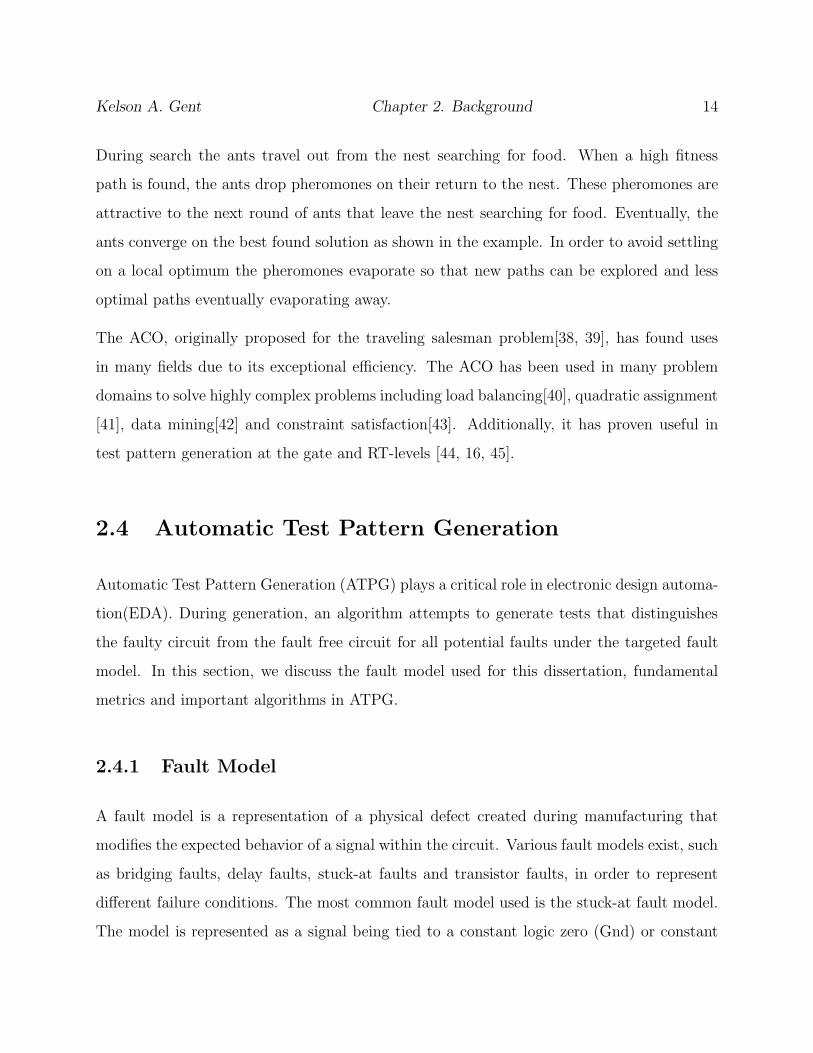
2.4 Automatic Test Pattern Generation
Automatic Test Pattern Generation (ATPG) plays a critical role in electronic design automa-
tion(EDA). During generation, an algorithm attempts to generate tests that distinguishes
the faulty circuit from the fault free circuit for all potential faults under the targeted fault
model. In this section, we discuss the fault model used for this dissertation, fundamental
metrics and important algorithms in ATPG.
2.4.1 Fault Model
A fault model is a representation of a physical defect created during manufacturing that
modifies the expected behavior of a signal within the circuit. Various fault models exist, such
as bridging faults, delay faults, stuck-at faults and transistor faults, in order to represent
different failure conditions. The most common fault model used is the stuck-at fault model.
The model is represented as a signal being tied to a constant logic zero (Gnd) or constant

Kelson A. Gent Chapter 2. Background 15
logic one(Vcc), as shown below in Figure 2.3.
������
���
���
���
��� ���
(a) Stuck-at 0 fault (b) Stuck-at 1 fault
Figure 2.3: Stuck-at Fault Model
The stuck-at fault model has a number of advantages including:
• High coverage of stuck-at faults allows for the detection of many types of physical
defects in practice;
• Independent of the manufacturing process;
• Total number of faults is linearly proportional to the size of the circuit;
• Many other fault models can be represented as a combination of two or more stuck-at
faults;
During ATPG it is typically assumed that only a single stuck-at fault exists at a given time.
In practice, however, multiple defects can exist on a single failing chip. Fortunately, it has
been shown that a test set that detects all single stuck-at faults also has a high probability
of detecting multiple fault failures[6]. For this work, we have used the stuck-at fault model
as the basis for our test generation.
2.4.2 Fault Coverage
Fault coverage is a metric used to assess the efficacy of a test set for a particular circuit
under test. Fault coverage is defined by the following equation.

Kelson A. Gent Chapter 2. Background 16
FaultCoverage (%) =Number of faults detected
Total number of faults× 100 (2.1)
Ideally, a test set achieves 100% fault coverage. In this case, a test set contains a pattern that
excites all faults in the circuit and propagates them to an externally visible signal. However,
for many circuits 100% coverage may not be feasible due to the existence of undetectable
faults. These faults arise from structures that mask the fault and prevent propagation. In
the presence of undetectable faults, a test set aims to have 100% coverage of all detectable
faults within the circuit, known as effective fault coverage. The effective fault coverage is
defined by the following equation.
FaultCoverage (%) =Number of faults detected
Total number of faults− number of undetectable faults× 100
(2.2)
Additionally, a test set with 100% coverage under a particular model may still not be com-
plete or adequate for fully testing a circuit. This is due to the fact that the model is not
a complete representation of all possible defects and the test set may fail to detect faults
under a different fault model.
2.4.3 State Justification
Verification in modern circuits is particularly difficult due to their size and complexity.
Finding test vectors to exercise deep, hard-to-reach states in the circuits operation is random
resistant and frequently requires significant designer input. As a result, state justification is
one of the most difficult problems in sequential ATPG and functional verification. In this
section, we define state justification and present several important definitions.
Given a circuit C with m inputs and n Flip-Flops, the input and present-state variables
are represented as a set X = {x0, ..., xm} and V = {V1, ..Vn}, respectively. The next-state

Kelson A. Gent Chapter 2. Background 17
variables are then represented by the set V ′ = {v′1, ..., v′n}. Where each member of the sets
is a logic value q ∈ {0, 1}.
From these sets, the circuit is then modeled as a finite state machine, FSM = (I, S, V0, T )
where I is the valid input set encoded from X , S is all possible states encoded by the present
state variables V , V 0 ∈ S is the initial state and T is the next state function.
To represent the circuit in a time frame t, we use X t and V t with the target final state
represented as V f . The finite state machine M can then be expanded to a directed graph
representation G(S,E), the State Transition Graph (STG), with the edge set E = {e|Vi, Vi ∈
S∃Xs.t.Vj = V ′
i = δ(Vi, X)}. A test vector can be represented as a list X i, X i+1, ...Xj =
X i...j where i ≤ j.
Based on the STG, the state justification problem can be formulated as a graph reachability
search, with the result being a directed path from V 0toV f in G(S,E). A path with length t
can be expressed as a sequence of inputs: X0...t that satisfy the equation:
V 0 ∧t−1∧
i=0
T (V i,W i, V i+1) ∧ V f
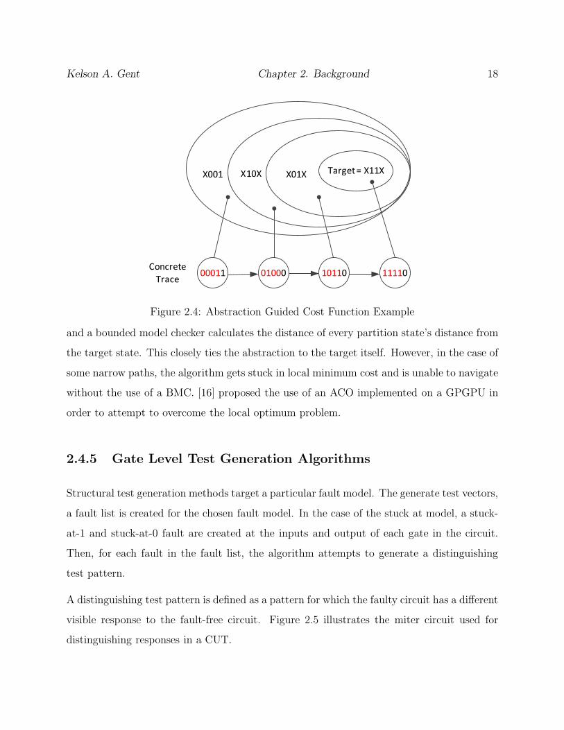
2.4.4 Abstraction Guided Search
In order to adequately handle the state explosion problem in state justification experienced
by formal methods, researcher have utilized hybrid methods that employ formal learning to
generate an abstraction that guides a stochastic search. These methods allow for significant
reduction in the time and memory required to compute a satisfying vector. One of the
primary methods used is a cost estimate generated from an abstraction of circuit behavior
[18, 46, 16]. Figure 2.4, illustrates the use of a cost function based on an abstracted state
and it’s applicability to state justification.
The cited works rely on a distance based cost function based on a partition of the circuit
state. Originally proposed by [18], distance guided navigation is proposed and is used during
simulation alongside a controlled hill-climbing metric. In [21], a set of partitions is created
Kelson A. Gent Chapter 2. Background 18
�������������
��� ���� �� �� ������
�����
Figure 2.4: Abstraction Guided Cost Function Example
and a bounded model checker calculates the distance of every partition state’s distance from
the target state. This closely ties the abstraction to the target itself. However, in the case of
some narrow paths, the algorithm gets stuck in local minimum cost and is unable to navigate
without the use of a BMC. [16] proposed the use of an ACO implemented on a GPGPU in
order to attempt to overcome the local optimum problem.
2.4.5 Gate Level Test Generation Algorithms
Structural test generation methods target a particular fault model. The generate test vectors,
a fault list is created for the chosen fault model. In the case of the stuck at model, a stuck-
at-1 and stuck-at-0 fault are created at the inputs and output of each gate in the circuit.
Then, for each fault in the fault list, the algorithm attempts to generate a distinguishing
test pattern.
A distinguishing test pattern is defined as a pattern for which the faulty circuit has a different
visible response to the fault-free circuit. Figure 2.5 illustrates the miter circuit used for
distinguishing responses in a CUT.

Kelson A. Gent Chapter 2. Background 19
The miter circuit contains two copies of the CUT, a fault free and a faulty copy. The faulty
copy has the target fault injected at the affected location. The primary inputs to both
circuits are tied together and the primary outputs are XORed to take the boolean difference.
During test generation, the algorithm attempts to find a set of inputs PI1−n such that, the
output of the miter circuit is 1. This indicates a that the fault-free and faulty circuits have
distinguishing outputs implying that the pattern detects the target fault.
����������
����
������ ����
����������� ��
� �� ���
Figure 2.5: Miter Circuit for ATPG
Some of the most influential work on structural ATPG includes the D-Algorithm [47], PO-
DEM [48], FAN [49], and SOCRATES [50]. Instead of utilizing a miter circuit, like shown
above, the D- Algorithm introduced the D notation for stuck at faults. The D-notation is a
5-value algebra that represents the two stuck-at faults as D = 1/0 (stuck-at-0) and D̄ = 0/1
(stuck-at-1). Therefore, the full value set that any given signal can take in a circuit is
{0, 1, X,D, D̄}. In these algorithms, a target fault is injected as either a logic D or D̄ and it
is considered detected when the algorithm is able to propagate the faulty value to a primary
output. in order to generate a pattern for a target fault, these algorithms deterministically
search for a pattern that excites the fault and propagates it to a primary output.
Additional improvements to combinational ATPG include fault dropping, and test set com-
paction methods. Fault dropping is a technique in which for each iteration of the ATPG
Kelson A. Gent Chapter 2. Background 20
engine, the test pattern generated is fault simulated to determine which other faults are
also detected by the pattern. The additionally detected faults are then dropped from the
search, so that the algorithm does not expend effort generating patterns for faults that were
already detected by a previous pattern. Test set compation is an attempt to minimize the
test application time by reducing the number of vectors required to cover all faults detected
by a given test set. Several techniques [51, 52, 53, 54, 55, 56, 57] have been proposed for
both static and dynamic compaction.
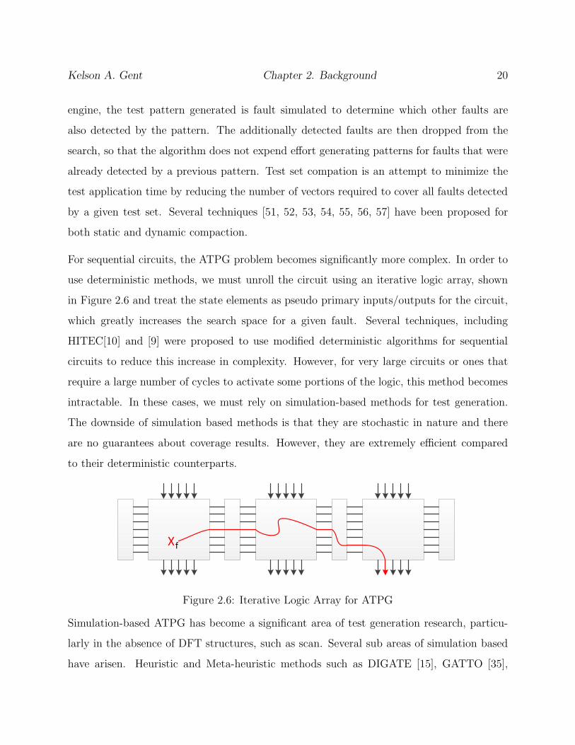
For sequential circuits, the ATPG problem becomes significantly more complex. In order to
use deterministic methods, we must unroll the circuit using an iterative logic array, shown
in Figure 2.6 and treat the state elements as pseudo primary inputs/outputs for the circuit,
which greatly increases the search space for a given fault. Several techniques, including
HITEC[10] and [9] were proposed to use modified deterministic algorithms for sequential
circuits to reduce this increase in complexity. However, for very large circuits or ones that
require a large number of cycles to activate some portions of the logic, this method becomes
intractable. In these cases, we must rely on simulation-based methods for test generation.
The downside of simulation based methods is that they are stochastic in nature and there
are no guarantees about coverage results. However, they are extremely efficient compared
to their deterministic counterparts.
��
Figure 2.6: Iterative Logic Array for ATPG
Simulation-based ATPG has become a significant area of test generation research, particu-
larly in the absence of DFT structures, such as scan. Several sub areas of simulation based
have arisen. Heuristic and Meta-heuristic methods such as DIGATE [15], GATTO [35],

Kelson A. Gent Chapter 2. Background 21
STRATEGATE [58, 59, 60, 61] and [62] use evolutionary and swarm inteligence based al-
gorithm. Logic simulation based techniques [63, 64] utilize properties in logic simulation to
attempt to fully exercise the circuit. Spectrum and compaction based techniques such as
[65], use signal analysis to aid in the generation of vectors. Sequential ATPG methods have
also been applied to verification and validation, such as [66, 67]. Additionally, sequential
and functional test generation research has also found applications in security domains, such
as in hardware trojan detection [68, 69, 70, 71]. As a result of the broad applicability of
functional and sequential tests, there has been significant research interest in high quality
efficient methods of test pattern generation. To address this, there has also been a push
to incorporate knowledge from the RTL [22, 72] to aid ATPG, which is one of the primary
themes covered in this dissertation.

Chapter 3
Semi-Formal Functional Test
Generation at the RTL
3.1 Chapter Overview
In this chapter, we present a semi-formal swarm intelligence tool for RTL function test
generation. The algorithm utilizes a SMT-based bounded model checker(BMC) and an ACO
to improve test generation targeting branch coverage. During compilation, a bounded model
checking instance is generated from the RTL source. Then, during the stochastic search, the
bounded model checker is used to attempt to expand the unexplored search frontier, aiding in
the navigation of narrow circuit paths. Additionally, an inductive reachability test is applied
to eliminate unreachable branches from the search space. This implementation has allowed
us to reach 100% coverage in several ITC99 benchmarks while maintaining or improving
performance over purely stochastic methods due to an increased convergence factor from the
BMC.
The rest of the chapter is organized as follows. A short introduction is given in Section 3.2.
A background of previous work for functional test generation at the RTL is given in Section
22

Kelson A. Gent Chapter 3. Semi-Formal Functional Test Generation at the RTL 23
3.3. Section 3.4 describes the methodology of the proposed algorithm. The experimental
results of the method are given in Section 3.5. Finally, a concluding summary conclude the
chapter in section 3.6.
3.2 Introduction
Functional test generation is a critical component of pre-silicon verification. Prior to chip
manufacturing, significant effort must be applied to ensure that the design description func-
tions as intended. In typical design flows, this process consists of a combination of random
and directed testing. Directed testing requires significant time from the designers in order to
generate good tests that effectively exercise their design. Additionally, as chips become more
complex, more directed effort is required as the level of coverage achievable from random test
drops. This effort and requirement for designer time has lead to a need for automated tools
to aid in the generation of functional tests that reach deep branches or states. Recently, sev-
eral tools [73, 44] have attempted to address the problem through the use of branch coverage,
originally proposed by [74, 75].
This chapter presents our methodology, which attempts to balance the tradeoffs between both
solutions. The method aims to maintain the high level of performance achieved through the
use of stochastic methods and assist in the navigation of narrow paths through the use of
formal methods. To accomplish this goal, during compilation, a bounded model checker is
extracted from the RTL source and represented as an SMT formulation. Then, utilizing a
fast RTL simulator, Verilator [76], we instantiate a swarm intelligence engine to do vector
generation based on simulation. During the stochastic search the BMC is invoked to aid in
the generation of vectors that expand the current search frontier and eliminate unreachable
branches from the search. Experimental results show that this method finds previously
unexercised branches and additionally provides a performance increase over previous state
of the art methods due to faster convergence on high quality vectors.

Kelson A. Gent Chapter 3. Semi-Formal Functional Test Generation at the RTL 24
The high-level description of the proposed algorithm is as follows. During the RTL compi-
lation to C++, a plug-in for Verilator static analyzes the RTL and extracts the functional
control flow graph (CFG). Then, the CFG is passed to a SMT-based transitional model of
the circuit is generated for use in the BMC. This stage of analysis is added as an additional
one-time cost alongside the RTL compilation. Following this analysis, a random simulation
search begins using the instrumented C++ created by Verilator. Several simulations are run,
each acting as an ant in the Ant Colony Optimization (ACO). After a set number of simula-
tion cycles, visited branches are analyzed and given a fitness score. After several iterations
of the ACO, highly visited branches are removed from the target function. This removal
provides a natural exploration frontier, which can be used as a launching point (e.g., initial
states) for formal methods. The circuit is unrolled for several cycles and the input conditions
at the end of each vector are added. The vectors generated by the BMC are appended to
the random vectors and the fitness function is updated accordingly. Then, BEACON begins
again with the updated fitness function.
3.3 Background
In this section, we present the background required for the implementation of this method.
Additionally, we cover relevant prior works in detail.
3.3.1 Satisfiability Modulo Theory
Satisfiability Modulo Theory (SMT) is a conjunction of theories for decision making and con-
straint satisfaction on first order logic. Although the general non-linear case for first order
logic is undecidable, many subcases are able to be solved. In particular, linear representa-
tions can be expressed as SAT and are therefore decidable with NP-complete complexity.
SMT solvers attempt to model the logic as an interpretation of the symbols with different
background theories. Some of these theories include, the theory of arrays, arithmetic theory
Kelson A. Gent Chapter 3. Semi-Formal Functional Test Generation at the RTL 25
and theory of lists. An introduction to the underlying theories is given by Microsoft Research
[77].
Modern solvers are categorized as either lazy or eager solvers. Eager solvers transform
the first order logic into a Boolean satisfiability instance and use a SAT solver to find an
assignment. Lazy solvers attempt to directly solve the theory only using SAT as necessary
and frequently use T-solvers, or specific theory solvers. Modern lazy solvers use an extension
of DPLL name DPLL(T) [78]. This has allowed for great efficiency gains in SMT solvers.
As a result, SMT solvers have become an attractive option for model checking and analysis
for problems that lend themselves to a first-order logical representation, such as software
analysis.
We use SMT as the basis of our BMC. SMT has a number of advantages over SAT for
processing RTL descriptions, including better solving speed for some equations and better
expressiveness for concepts such as arrays, and word level modeling. Limited support for
some second order and undecidable theories also allow us to express concepts such as multi-
plication and modulus operations at a higher level of abstraction than the actual structural
representation required by SAT.
3.3.2 Bounded Model Checking
Based on the CFG, we can generate a single time frame SMT representation of the cir-
cuit. This translation is done by doing a data flow analysis in the form of a single static
assignment(SSA) analysis. The SSA form of the Verilog RTL is then used to generate the
transition condition for a single timeframe. The transition condition is represented as nested
if-then-else(ITE) formulas derived from the branch nodes of the CFG, based off the method
proposed in [79] and [80]. This representation is then passed to a SMT solver, Microsoft
Research’s Z3 [81]. Additionally, all registers are represented as pseudo-primary inputs(PPI)
and pseudo-primary outputs(PPO), such that at the end of a time frame the final values
of a variable are written to a PPO and then passed to the corresponding PPI of the next

Kelson A. Gent Chapter 3. Semi-Formal Functional Test Generation at the RTL 26
timeframe. This allows for standard unrolling in the creation of an iterative logic array. An
example of the conversion to SMT can been seen below in Figure 3.1.
if (reset == 1'b’1)
begin
done=1'b0;
count = 10'b0
end
else
begin
if(count < 10'hff)
begin
count = count + 1;
end
end
SMT formula for count
IF(reset[i] == 1'b’1) THEN
count[i] = 10'h000
ELSE IF (count[i] < 10'h0ff)
THEN
count[i] = count[i-1]+1
ELSE
count[i] = count[i-1]
Figure 3.1: SMT transition formula and corresponding Verilog
Based on this single time-frame instance, we can unroll our circuit to form a BMC, outlined
by Clarke, Beine, et al. [82]. The general BMC formula used is given below.
M =∨
I(S0) ∧∧
T (si, si+1) ∧∧
P (si)
Such that, I(S0) is a possible initial state, T (si, si+1) is the transition statement from state
i to state i + 1 and P (s) is the property to be proven in a given state i, and i is bound by
some upper limit k.
For improving branch coverage, the properties are the activation of an instrumentation point.
For our work, the instrumentation points are counters, initialized to 0. Therefore, we can
add a constraint such that the instrumentation point is greater than 0 in the final time frame
to guarantee that a branch has been covered during execution.
3.3.3 Prior Work
Heuristic based functional test/stimuli generation has had several influential prior works.
Corno et al, proposed a genetic algorithm based solution [83]. Their procedure interacts with

Kelson A. Gent Chapter 3. Semi-Formal Functional Test Generation at the RTL 27
the simulator via the trace file and attempts to generate a trace with maximum coverage.
However, due to the lack of guidance the algorithm cannot identify and target difficult-to-
reach branches, leaving many hard-to-reach corner cases remain uncovered.
Prior algorithms have utilized several techniques, in order to attempt to reach new branches
within the RTL source. HYBRO [73], utilizes a hybrid technique that extracts conditions,
guards, from concrete executions and attempts to mutate the guards using a SMT-solver to
discover new possible execution paths. This method is highly reliant on calls to the SMT
solver for exercising new branch paths. These calls are computationally expensive which
greatly limits the number of vectors that can be analyzed using this method. Therefore,
circuits which require extremely long vector lengths to exercise some branches are not effec-
tively tested by HYBRO due to path explosion while attempting to find feasible mutations.
Another work, BEACON [44] utilizes a purely stochastic evolutionary swarm intelligence
algorithm based on an ACO to attempt to address the problem of branch coverage at the
RTL. However, due to it’s stochastic nature, the existence of narrow paths cause significant
increases in execution time in order to converge on vectors that navigate the path with no
guidance. Additionally, the algorithm may target or highly weight branches in its fitness
function that are unreachable.
Several other methods [18, 84, 21, 45] for functional test generation have been previously
proposed. Most of these techniques are abstraction-based and use semi-formal methods of
exploration. However, circuit abstraction has several inherent problems. Due to the nature
of the the abstraction, there is an inherent information loss associated with the model. The
information loss tends to have issues with dead-end abstract states that are scored well but
provide a false path to necessary corner case states. Also, the methods in [21, 45] rely on only
gate-level information so it is significantly more difficult to extract an accurate abstraction.

Kelson A. Gent Chapter 3. Semi-Formal Functional Test Generation at the RTL 28
3.4 Methodology
While previous stochastic methods can scale better on larger circuits, they face hurdles when
trying to reach hard-to-reach corner cases. This work impacts the aforementioned two-step
stochastic search process: First, the CFG extraction and the BMC generation are added
as an additional step in preprocessing, and second, the use of the BMC is added into the
guidance framework.
During preprocessing, the Verilog circuit description is translated by Verilator into a static
C++ cycle-accurate simulation library. During the conversion, Verilator instruments the
code for each branch and a database for the instrumentation points, which can serve as
monitors for path traversal and the number of times each branch has been visited. Following
the generation of the CFG, the BMC is also instantiated during the preprocessing step.
��������������
�����
����� ���� ����
���� �� !
"��#�� ����$%
&' ��$% ���(
)*#���
*%��������
+�# ��$��
����$%,
-�������
�.*�������/01!
+�#
+2��2� 3���
4��������,
5
6
56)*#��� 6���
Figure 3.2: Flow graph for hybrid framework
The addition of the BMC is shown in Figure 3.2. During the stochastic search using the ACO,
the pheromone map is initialized on the coverage database and assigned a constant initial
value. A colony of K ants is set-up, starting from the given initial state S0. Each ant then

Kelson A. Gent Chapter 3. Semi-Formal Functional Test Generation at the RTL 29
stochastically simulates a pre-determined number cycles, Nc, and updates the pheromone
map based on this traversal. The deterministic search (BMC) is launched immediately
preceding the ant evolution in the local search. This starting states of the BMC is tied to
a set of high-fitness states derived from the frontier, and the unrolling bound is determined
based on the complexity of the circuit and the number of uncovered points remaining. The
description of BMC generation is detailed in Section 3.4.3. After the BMC call, the rest of
the algorithm continues, and local search terminates when no more branches are uncovered
for a set Nr number of rounds. Once this occurs, the algorithm assumes that there are no
more branches to be uncovered within Nc cycles of simulation from S0. In order to extend
the search, we update the set of initial states with states Si, that have a high fitness score.
The local search then repeats. Once a steady state is reached such that no new high fitness
states found or no new branches are uncovered, we terminate. For reference, the pseudo-code
for the stochastic algorithm is shown in Algorithm 1.
Algorithm 1 Stochastic Search
1: trim unreachable branches2: generate initialize pheromone map φ3: for all rounds r = 1 to Nr do
4: set the initial states to nest S0
5: for all ants k = 1 to K do
6: random generate vectors with length Nc
7: local search()8: end for
9: if all branches are covered || sets = ∅ then10: RETURN11: else
12: S0 = select(sets)13: sets = ∅ {clear the stack}14: end if
15: end for

Kelson A. Gent Chapter 3. Semi-Formal Functional Test Generation at the RTL 30
3.4.1 Control Flow Graph Extraction
In order to extract the CFG [27] during source-to-source compilation, we utilize a plug-
in for Verilator based off the instrumentation analysis already available. At each branch,
Verilator adds a counter to the compiled source that increments whenever the execution
trace activates the branch condition. An example of the graph created during compilation
is shown in Figure 3.3. Each numbered node is correlated with an added instrumentation
point. These points are mapped directly to nodes in the extracted CFG, represented as a
hierarchical graph structure with parent and child relationships stored at each node.
1. if (ru1 == 1'b1){
2. if (fu1 == 1'b0){
3. coda3 <= coda2;
4. coda2 <= coda1;
5. coda1 <= coda0;
6. coda0 <= `U1;
7. }
8. }
9. else if (ru2 == 1'b1){
10. if (fu2 == 1'b0){
11. coda3 <= coda2;
12. coda2 <= coda1;
13. coda1 <= coda0;
14. coda0 <= `U2;
15. }
16. }
17. else if (ru3 == 1'b1){
18. if (fu3 == 1'b0){
19. coda3 <= coda2;
20. coda2 <= coda1;
21. coda1 <= coda0;
22. coda0 <= `U3;
23. }
24.}
1
2
3
4
5
6
variable
assign
variable
assign
variable
assign
Figure 3.3: (a) b3 source segment (b) the corresponding CFG.
Since Verilator’s instrumentation system already creates a unique identifier for each branch,
it was used to extract the full CFG and dependent variable assignments. During extraction,

Kelson A. Gent Chapter 3. Semi-Formal Functional Test Generation at the RTL 31
we find the least fixed-point of variables such that all controlling statements can be fully
evaluated, effectively minimizing the size of the model. This fixed point can be calculated
using the following method.
Let G be a graph such that each vertex v ∈ V (G) represents a variable in a circuit. Let Ctrl
be a set such that Ctrl ⊆ V (G) where each element of Ctrl is a variable used in a control
structure in the circuit. For u, v ∈ V (G), (u, v) ∈ E(G) if there exists an assignment in the
circuit such that v is used in a function that assigns u. The least fixed point f can be defined
such that:
f = µZ.(∀e ∈ V (G), e ∈ Ctrl ∨ ∃(u, e) ∈ E(G), u ∈ Z)
During this fixed point analysis, we also add each relevant assignment to the CFG. We do
this by attaching each assignment to its covering instrumentation point node, as they are
found. Additionally, each branch control statement is also added to the associated node in
the directed graph.
Given the Verilog construct in Figure 3.1 above, the fixed point variables are reset and count.
In the first pass of the fixed point, reset and count are added to the set Z since they are
variables in control statements. Since no variables assign values to these variables, the fixed
point is complete and done is excluded from the extraction.
3.4.2 Unreachable Branch Identification
The BMC can also be used to trim unreachable states. We set up an inductive proof in
order to identify branches targets that are unreachable from the initial state. We generate
a property P (i), such that when P (i) is true, the branch path as been exercised in time-
frame i. The base case for the proof is a check that the property is not satisfied in a valid
initial state. To check this, we start from an unspecified state and apply a known reset or
initialization sequence and check P (0) in the initialized time-frame. The inductive case is to
unroll the circuit for two time-frames. We relax the initial state and assert a constraint such

Kelson A. Gent Chapter 3. Semi-Formal Functional Test Generation at the RTL 32
that the property is false in the first time-frame and check if there exists a vector such that
the property is satisfied in the second timeframe n + 1. If either the base or the inductive
case returns satisfiable, then the state is potentially reachable from the target. Otherwise,
we mark the node as unreachable and remove it from our colony’s fitness function. This
is a one time operation that stops the algorithm from searching for provably unreachable
branches. This removes isolated nodes in the CFG and nodes with conflicting conditions in
the model, which eliminates repeated calls to the simulation engine and BMC searching for
these nodes.
3.4.3 Local Search
The proposed hybridization will affect the stochastic search. However, since this local search
consumes the bulk of the execution time in the test generator, the introduction of a deter-
ministic BMC must be carefully managed. The basis of the local search is an ACO similar to
the one described in [44]. However, one significant step is added called the frontier expansion.
The overall flow of the local search is shown in the pseudo-code in Algorithm 2. Additionally,
the pheromone deposit function is changed to weight traversals that visit branches with large
numbers of uncovered children in the CFG.
As proposed, frontier expansion is a deterministic search following the local stochastic search.
Fundamentally, the ants in our algorithm are randomly searching the CFG of the circuit
during random simulation. Due to this, at the end of a round, r, there is a naturally formed
limit or ”frontier” between visited and unvisited branches. During the expansion, we utilize
the generated BMC to attempt to find direct paths to unvisited paths that are close to nodes
we have already visited. To start this search, we select initial states for the BMC from high
fitness states found during the ACO search. These states make up the∨
I(S0) clause in the
BMC. Additionally, the logical propositions for coverage of all unvisited branches are added
in disjunction to form the property clauses P (Si) in the BMC. The BMC then attempts to
find a satisfying solution. If a solution is found, then it is inserted into the vector immediately

Kelson A. Gent Chapter 3. Semi-Formal Functional Test Generation at the RTL 33
Algorithm 2 Local Search
1: while rounds n < Nr do
2: for all ants k = 1 to K do
3: for all cycles c = 1 to Nc do
4: eval() { the evaluation function}5: record the trace using instrumented code6: if new branch || fitness(Sk
c ) > threshold then
7: sets ← Skc
8: end if
9: deposit pheromone on the trace10: end for
11: end for
12: update pheromone()13: frontier expansion()14: evolve ant()15: if new branch is covered then
16: n = 0 { clear the rounds counter}17: else
18: ++n19: end if
20: end while
following the trace leading to the high fitness state. These states are also stored in order to
be used during ant evolution, discussed in Section 3.4.4.
3.4.4 Ant Evolution
Evolution of the ants was a primary factor in the success of the stochastic algorithm, because
the highest fitness state may not occur at the end of the vector. As a result, the ant with
the best fitness may have generated vectors that actually lead us away from the target.
Therefore, a cut based evolution method was employed to prune the vectors of wasteful and
potentially undesirable vectors. The vectors are selected for cut through a stochastic fitness
weighted function.
Once a cut point is selected, two vectors are combined utilizing the method shown in Figure
3.4. For each cut in a vector, the two sections can be labeled as an impeding section and a

Kelson A. Gent Chapter 3. Semi-Formal Functional Test Generation at the RTL 34
progressive section shown in the dotted circle on Figure 3.4(a). Once the two cuts are made,
a crossover operation is performed to combine the vectors. The two children formed by this
operation are shown in Figure 3.4(b).
(a) (b)
Cut Points Pad
Section
Figure 3.4: Vector Crossover (a) parents (b) children.
In the purely stochastic method, pad space was filled to the original vector length with
additional random input. However, we propose that this method is sub-optimal because it
may lead the cut vector further away from the target, uncovered branches. As a substitute,
we propose that the deterministic vectors generated during frontier expansion are ideal for
padding. This is due to the fact that if there are vectors generated during the deterministic
search, they are guaranteed to be vectors that improve the overall search fitness. In the
event that no vectors are generated and the fitness expansion returns as unsatisfiable for all
remaining branches, the algorithm can fall back to random generation.
3.5 Results
The BEACON extension and model extraction plug-in were developed on an Intel Core
[email protected] with 8 cores and 16GB of memory running Ubuntu 12.04. Experiments
utilized a single core and were conducted on a set of ITC99[85] circuits to assess their
performance relative to prior works and BEACONS original runtimes. The characteristics of
the designs tested are given in Table 3.1. Additionally, as representatives of general sequential
logic, many of the ITC99 [85] benchmarks circuits have hard-to-reach states(control states),
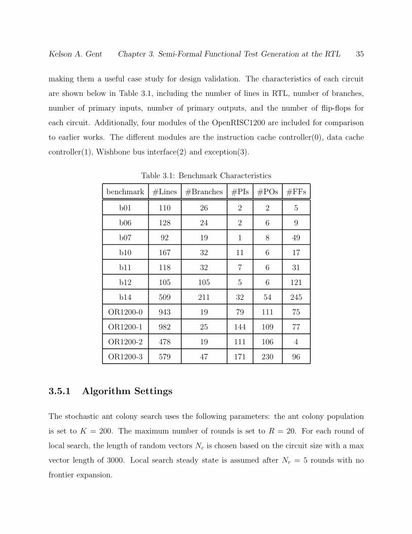
Kelson A. Gent Chapter 3. Semi-Formal Functional Test Generation at the RTL 35
making them a useful case study for design validation. The characteristics of each circuit
are shown below in Table 3.1, including the number of lines in RTL, number of branches,
number of primary inputs, number of primary outputs, and the number of flip-flops for
each circuit. Additionally, four modules of the OpenRISC1200 are included for comparison
to earlier works. The different modules are the instruction cache controller(0), data cache
controller(1), Wishbone bus interface(2) and exception(3).
Table 3.1: Benchmark Characteristics
benchmark #Lines #Branches #PIs #POs #FFs
b01 110 26 2 2 5
b06 128 24 2 6 9
b07 92 19 1 8 49
b10 167 32 11 6 17
b11 118 32 7 6 31
b12 105 105 5 6 121
b14 509 211 32 54 245
OR1200-0 943 19 79 111 75
OR1200-1 982 25 144 109 77
OR1200-2 478 19 111 106 4
OR1200-3 579 47 171 230 96
3.5.1 Algorithm Settings
The stochastic ant colony search uses the following parameters: the ant colony population
is set to K = 200. The maximum number of rounds is set to R = 20. For each round of
local search, the length of random vectors Nc is chosen based on the circuit size with a max
vector length of 3000. Local search steady state is assumed after Nr = 5 rounds with no
frontier expansion.

Kelson A. Gent Chapter 3. Semi-Formal Functional Test Generation at the RTL 36
Parameters α and β for pheromone and visibility are set to 1.0 and 0.5, respectively. Setting
β to 1 results in short testing vectors which cannot cover some branches. In contrast, when
β = 0.0, cut points are selected too close to the end of a vector, which causes more redundant
vectors and runtime overhead. Therefore, we pick β = 0.5 as a compromise. The initial
amount of pheromone was set to 1000 and the maximum amount of pheromone released by
one ant is Q = 100. Pheromone evaporation rate ρ was set to 10%.
The BMC uses a variable maximum depth unrolling depending on the round R, such that
the maximum depth increases from 5 to 10 time frames. The unroll depth is kept small in
order to minimize execution time.
3.5.2 Branch Coverage
Our algorithm significantly increases branch coverage, and in a number of cases reaches
100% coverage through the use of inductive reachability proofs. Additionally, compared
to prior algorithms, we retain a high level of performance, frequently showing significant
improvements in speed. The branch coverages are given below in Table 3.2.

Kelso
nA.Gent
Chapter
3.Sem
i-Form
alFunctio
nalTest
Genera
tionattheRTL
37Table 3.2: Branch Coverage and Comparison with Prior Techniques
BenchBranch Coverage %
UnreachableRun Time(s) Speedup Over
HYBRO BEACON Ours HYBRO BEACON Ours HYBRO BEACON
b01 94.44 100.00 100.0 1 0.07 0.0024 0.0020 35.00 1.2
b06 94.12 95.83 100.00 1 0.1 0.0054 0.02s 5.00 0.27
b07 NA 90.00 95.00 1 NA 0.37 0.41s NA 0.90
b10 96.77 93.75 100.00 1 52.14 11.40 3.12 16.71 3.6
b11 91.30 96.88 96.88 1 326.85 11.95 4.2 77.82 2.84
b12 NA 98.09 97.1 1 NA 111.42 69.6 NA 1.6
b14 83.50 91.94 93.4 2 301.69 204.65 94.2 3.20 2.17
OR1200-0 93.75 89.47 89.47 0 37.73 4.38 2.82 13.38 1.55
OR1200-1 96.30 92.00 92.00 0 21.9 4.87 2.75 7.96 1.77
OR1200-2 100.00 100.00 100.00 0 302.67 2.85 2.82 107.33 1.01
OR1200-3 96.61 97.87 97.87 0 287.62 27.35 6.4 44.94 4.27

Kelson A. Gent Chapter 3. Semi-Formal Functional Test Generation at the RTL 38
Our algorithm shows speedups despite the introduction of a formal solver to the tool. This
speedup occurs primarily because the BMC yields a faster convergence to steady state cover-
age values, leading to earlier termination. Based off the initial results, the frontier expansion
allows the simulation to reach steady state convergence in fewer rounds. For several of our
benchmarks, we are able to reach complete coverage for the benchmark. In b06, we are able
to find that the only branch left uncovered by BEACON is unreachable under non-faulty
operation. Additionally, in b10 The BMC allows the algorithm to uncover an additional
branch and finds the remaining branch to be unreachable providing complete coverage for
the benchmark. Further improvement comes for benchmark b14, which in addition to prov-
ing unreachability for 2 branches, the BMC finds the vectors to reach an additional branch.
In a number of cases, due to the short unrolled length, the BMC is limited based on the
performance of the simulation based search engine. This is evident in the OR1200 blocks
in which no significant improvement in coverage is seen. However, the introduction of the
BMC and convergence factors yields a significant speedup. Also, in b12, we saw a slight
reduction in coverage because the algorithm converged to the high value of coverage in much
fewer rounds and failed to touch two previously covered branches.
3.6 Chapter Summary
In this chapter, we proposed merging a stochastic search technique with limited scope deter-
ministic search for design validation in RTL based on branch coverage. To improve perfor-
mance, we introduce deterministic methods to help the swarm intelligence algorithm navigate
highly specific execution paths. In order to accomplish this hybridization, we outlined the
graph analysis plug-in for Verilator to do the circuit model extraction during compilation.
Additionally, we described the implementation of our SMT-based BMC. Finally, we proposed
the deterministic search method integration and analyzed the performance of the combined
algorithm. This analysis shows that formal methods can improve the overall coverage of the

Kelson A. Gent Chapter 3. Semi-Formal Functional Test Generation at the RTL 39
algorithm, and in many cases can reduces the overall execution time, due to search space
reduction and faster steady state convergence in the search algorithm.

Chapter 4
Dual-Purpose Mixed-Level Test
Generation Using Swarm Intelligence
4.1 Chapter Overview
In this chapter, we present a method for simultaneously target the RTL and gate level
descriptions of a circuit under test. High-level test generators often miss the low- level de-
tails, thus missing the detection of some gate-level faults. On the other hand, gate-level
test generators miss the high-level path traversal knowledge to more effectively traverse the
state space. By co-simulating the RTL and gate level, we can create a feedback cycle for
test generation that allows us to quickly generate high quality vectors for both levels with
low computational costs, even in the presence of deep hard-to-reach states. In particular,
for hard-to-test circuits such as the ITC’99 circuit b12, >98% branch coverage and >90%
stuck-at coverage are achieved, vastly improving over other state of the art non-scan tools.
Additionally, no design-for-test features, such a scan flip-flops, are required for the applica-
tion of these vectors. Therefore, the vectors generated are particularly useful for at-speed
testing.
40

Kelson A. Gent Chapter 4. Mixed-Level Test Generation 41
The rest of the chapter is organized as follows. An introduction is given in Section 4.2. A
background of previous work for functional test generationat the RTL is given in Section
4.3. Section 4.4 describes the methodology of the proposed tool. The experimental results
of the method are given in Section 4.5. Finally, a concluding summary conclude the chapter
in section 4.6.
4.2 Introduction
Following Moore’s Law, modern microprocessor designs have doubled in transistor count
approximately every 18 months. This dramatic rise, coupled with the exponential complex-
ity of deterministic ATPG with relation to circuit size, has caused significant difficulty for
sequential test generation. In terms of reducing manufacturing test complexity, (full) scan
has been the de-facto standard to help alleviate the burden. However, defects in the deep
submicron are increasing failures that scan-based tests may not capture, and those escaped
defects are causing chip failures in the functional mode. On the other hand, both pre- and
post-silicon validation demand effective functional vectors to exercise the circuit. In order
to minimize the test generation cost, stochastic, abstraction-guided methods have been pro-
posed in the past. However, such methods often fail to exercise hard-to-detect faults due
to their lack of knowledge about either the high-level or low-level structural information.
Nevertheless, there is merit in both high-level and low-level test generators. For example,
the register transfer level (RTL) has several advantages over the gate level in terms of word-
level operations (both logical and mathematical) and control information such as if-else and
case statements. On the other hand, the gate-level structural information has detailed in-
formation that can better represent specific low-level defects. Therefore, it is judicious to
include various levels of abstraction when targeting the difficult problem of sequential test
generation.
In this chapter, we propose a method for addressing the sequential test generation problem
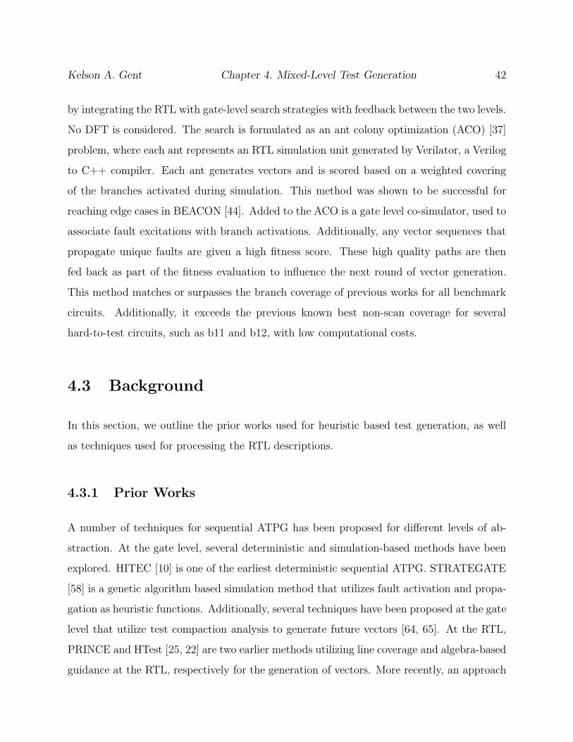
Kelson A. Gent Chapter 4. Mixed-Level Test Generation 42
by integrating the RTL with gate-level search strategies with feedback between the two levels.
No DFT is considered. The search is formulated as an ant colony optimization (ACO) [37]
problem, where each ant represents an RTL simulation unit generated by Verilator, a Verilog
to C++ compiler. Each ant generates vectors and is scored based on a weighted covering
of the branches activated during simulation. This method was shown to be successful for
reaching edge cases in BEACON [44]. Added to the ACO is a gate level co-simulator, used to
associate fault excitations with branch activations. Additionally, any vector sequences that
propagate unique faults are given a high fitness score. These high quality paths are then
fed back as part of the fitness evaluation to influence the next round of vector generation.
This method matches or surpasses the branch coverage of previous works for all benchmark
circuits. Additionally, it exceeds the previous known best non-scan coverage for several
hard-to-test circuits, such as b11 and b12, with low computational costs.
4.3 Background
In this section, we outline the prior works used for heuristic based test generation, as well
as techniques used for processing the RTL descriptions.
4.3.1 Prior Works
A number of techniques for sequential ATPG has been proposed for different levels of ab-
straction. At the gate level, several deterministic and simulation-based methods have been
explored. HITEC [10] is one of the earliest deterministic sequential ATPG. STRATEGATE
[58] is a genetic algorithm based simulation method that utilizes fault activation and propa-
gation as heuristic functions. Additionally, several techniques have been proposed at the gate
level that utilize test compaction analysis to generate future vectors [64, 65]. At the RTL,
PRINCE and HTest [25, 22] are two earlier methods utilizing line coverage and algebra-based
guidance at the RTL, respectively for the generation of vectors. More recently, an approach
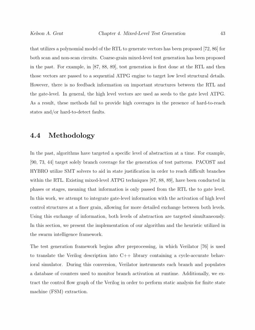
Kelson A. Gent Chapter 4. Mixed-Level Test Generation 43
that utilizes a polynomial model of the RTL to generate vectors has been proposed [72, 86] for
both scan and non-scan circuits. Coarse-grain mixed-level test generation has been proposed
in the past. For example, in [87, 88, 89], test generation is first done at the RTL and then
those vectors are passed to a sequential ATPG engine to target low level structural details.
However, there is no feedback information on important structures between the RTL and
the gate-level. In general, the high level vectors are used as seeds to the gate level ATPG.
As a result, these methods fail to provide high coverages in the presence of hard-to-reach
states and/or hard-to-detect faults.
4.4 Methodology
In the past, algorithms have targeted a specific level of abstraction at a time. For example,
[90, 73, 44] target solely branch coverage for the generation of test patterns. PACOST and
HYBRO utilize SMT solvers to aid in state justification in order to reach difficult branches
within the RTL. Existing mixed-level ATPG techniques [87, 88, 89], have been conducted in
phases or stages, meaning that information is only passed from the RTL the to gate level.
In this work, we attempt to integrate gate-level information with the activation of high level
control structures at a finer grain, allowing for more detailed exchange between both levels.
Using this exchange of information, both levels of abstraction are targeted simultaneously.
In this section, we present the implementation of our algorithm and the heuristic utilized in
the swarm intelligence framework.
The test generation framework begins after preprocessing, in which Verilator [76] is used
to translate the Verilog description into C++ library containing a cycle-accurate behav-
ioral simulator. During this conversion, Verilator instruments each branch and populates
a database of counters used to monitor branch activation at runtime. Additionally, we ex-
tract the control flow graph of the Verilog in order to perform static analysis for finite state
machine (FSM) extraction.

Kelson A. Gent Chapter 4. Mixed-Level Test Generation 44
789:;<;= >7?
@;A<B9
C;D;98<EBD
FDE<E8GEH8<EBD
I<89<
I<89< 8D<J K9BL
D;J< MINO
C;D;98<; <89:;<J
PD= GBA8G
J;89AQR
C8<; ?;S;G
TD8GUJEJ
PD=
VW=8<;
XQ;9BLBD;J
7;9LED8<;R
Y
Z
YZVW=8<; Z;J<
Figure 4.1: Algorithm Flow
The flow for our test generation is shown in Figure 4.1. During initialization, a database of
pheromones is established for each branch φ(b) and the pheromone is initialized to a constant
value. Additionally, the gate level circuit is read in, a database of faults is established, and
the fault simulator is initialized. Then, a colony of K ants is created and each ant randomly
generates an initialization vector. The ants then perform an initial RTL simulation from the
given initial state S0. After the initial simulation, the algorithm generates a target from the
unseen branches and begins vector generation. Following a round of RTL vector generation,
the vectors are scored according to the fitness function and high-fitness vectors are passed
to the gate-level. At the gate level, the fitness values of all ants are updated based on fault
activation. This process continues until no new faults or branches are uncovered for a set
Nr number of rounds. Once this occurs, the algorithm assumes that the colony has reached
steady state within Nc cycles from S0 and terminates. The pseudo-code of the colony is
shown below in Algorithm 3.

Kelson A. Gent Chapter 4. Mixed-Level Test Generation 45
Algorithm 3 ATPG Engine
1: initialize pheromone map φ2: initialize fault simulator3: extract branch FSM4: for all rounds r = 1 to Nr‘1 do
5: set the initial states to nest S0
6: for all ants k = 1 to K do
7: local search()8: end for
9: if all faults covered || sets = ∅ then10: RETURN11: else
12: S0 = select(sets)13: sets = ∅ {clear the stack}14: end if
15: end for
4.4.1 Finite State Machine Extraction
At the RTL, the FSM for the circuit is often explicitly declared. Additionally, each state
in the machine is typically associated with a single branch coverage statement. In order to
associate the branches, we utilize a static analysis method on the CFG extracted by Verilator.
CFGs of Verilog descriptions are acyclic within a given cycle, with a single entry and exit
point. Within a control flow graph, FSMs are defined by several characteristics: a set of
branches controlled by a single variable, such that only one branch can be active in a given
cycle and the assignments within the branch define the controlling variable in the next cycle.
In order to extract relationships between these branches, each exclusive branch within the
CFG is established as a node in the FSM and examined for potential assignments to the
controlling variable. During the examination of a node, N , if there exists an assignment
such that the controlling variable can be evaluated to a constant, then the constant value
is applied and the resulting activation is established as a successor to the current branch.
Additionally, the edge between them is defined as the necessary branch activations required
to reach the given assignment. An example of this process is shown on a simple write back
cache machine in Figure 4.2.

Kelson A. Gent Chapter 4. Mixed-Level Test Generation 46
������������
�������� ������������
���������������������������
������������������ !�"���#
$���������%����������#�����������
&�����������������' !�"���#
(������ !��������
)�������������*%���������
+������������������ �����"���#
�,���������#
�������' !��������
����������������*%���������
��������������������� �����"���#����
�����������%�����������-�������
�$������������������ !�"���#
�&����������#
�(�����#����
[\]^
_ ` aa
b
c
d a_
aee f ab
g ac
^hi
Figure 4.2: Control Flow Example
The three branches in Figure 3.3 that make up the FSM are at lines 2,7 and 11. Consider the
branch at line 2, there are two constant assignments at lines 4 and 5. These assignments set
the state variable to MOD and UNMOD, which activate branches 7 and 11 respectively,
and require branches 2, 3 and 2, 5 to be applied. The final branch FSM for Figure 3.3 is
shown below in Figure 4.3
4.4.2 Identifying Critical Nodes
To effectively utilize the extracted FSM, we attempt to identify critical nodes. These nodes
are embedded within cycles in which incorrect decisions will lead us away from nodes that
contain uncovered branches. For a given target (uncovered branch) t, a set of critical nodes
within the FSM can be computed at run time in the following manner. We first map t’s
location in RTL to a single node within the branch abstraction graph, G. The targets
abstract node, n, is the node in G whose associated branch is a necessary condition for
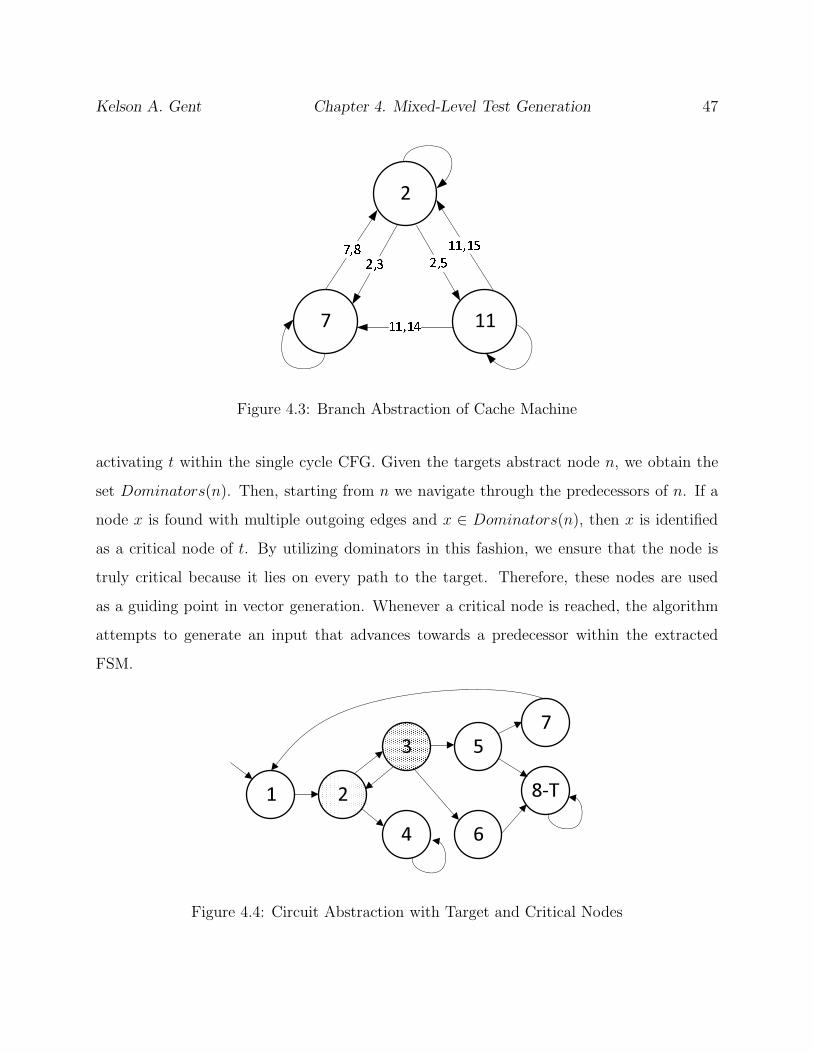
Kelson A. Gent Chapter 4. Mixed-Level Test Generation 47
� ��
�
jkl
mmkmn
okp
jkq
mmkml
Figure 4.3: Branch Abstraction of Cache Machine
activating t within the single cycle CFG. Given the targets abstract node n, we obtain the
set Dominators(n). Then, starting from n we navigate through the predecessors of n. If a
node x is found with multiple outgoing edges and x ∈ Dominators(n), then x is identified
as a critical node of t. By utilizing dominators in this fashion, we ensure that the node is
truly critical because it lies on every path to the target. Therefore, these nodes are used
as a guiding point in vector generation. Whenever a critical node is reached, the algorithm
attempts to generate an input that advances towards a predecessor within the extracted
FSM.
�
�������������������������������������������������������������������������������������������������������������������������������������������������������������������������������������������������������������������������������������������������������������������
�
�������������������������������������������������������������������������������������������������������������������������������������������������������������������������������������������������������������������������������������������������������������������
�
�
�
�
��
Figure 4.4: Circuit Abstraction with Target and Critical Nodes
Kelson A. Gent Chapter 4. Mixed-Level Test Generation 48
Consider an example graph shown in Figure 4.4. Let the target be node 8. The decision
nodes along the path from the entry to the target are those nodes with more than one
successor node, which are listed in Sdecide = {2, 3, 5}. The set of dominators of the target
can be easily computed to be Dom8 = {1, 2, 3}, because they lie on every path from the
entry node 1 to node 8. Therefore, based on the procedure explained above the set of critical
nodes for the given target, the set of critical nodes is Scrit = Sdecide ∩ Dom8 = {2, 3}. We
will construct the path-activation abstraction for this set, Scrit.
4.4.3 Vector Generation
The vector generation is done with the aid of both RTL-level branch coverage and gate-level
fault coverage. The algorithm first utilizes the extracted FSM to aid with generation for
hard to reach states. At the beginning of each round, the set of uncovered branches in the
FSM, Suncov, is used to randomly assign a target for each ant. Then, the FSM is analyzed
by each ant to determine the distance of each node in the FSM to the target. When a target
is assigned, each ant also calculates the critical nodes to reach that target based on the
procedure described in Section 4.4.2. Following RTL vector generation, the ants are handed
to the gate-level fault simulator to update the fitness values and the next round begins. This
flow is shown below in Algorithm 4.
At the beginning of test generation, each ant checkpoints their state so it can be restored
during the stochastic search and obtains the critical nodes for its target. Each ant then
generates and applies a random vector V . Following simulation the branch activation trace
is recorded, if the trace matches a critical node then the trace is applied to the abstraction
graph G to find the expected branch activations in the next cycle. A vector that advances
the abstraction towards the target is saved as a quality vector and added to the ants test
sequence. If the vector fails to advance the target within the abstraction, the ant attempts
to apply previously generated successful vectors. If no previously vectors exist, or they fail
to advance towards a good state, the ant falls back to random generation, in which the ant

Kelson A. Gent Chapter 4. Mixed-Level Test Generation 49
Algorithm 4 Ant Search with Targeted Input Generation
1: while rounds n < Nr do
2: Sbranch = uncovered branches()3: for all ants k = 1 to K do
4: set target(ants, Sbranch)5: calculate critical nodes()6: for all cycles c = 1 to Nc do
7: generate input()8: record the trace using instrumented code9: deposit pheromone on the trace10: end for
11: end for
12: update pheromone()13: fault simulate()14: sets = select ants()15: if new branch is covered then
16: n = 0 { clear the rounds counter}17: else
18: ++n19: end if
20: end while
repeatedly generates random inputs until an advancing input is found or until a timeout is
reached.
As an example of use of critical nodes, consider the circuit b12. The circuit is an imple-
mentation of a game system where the player must guess a sequence of random generated
numbers. There are 2 significant properties, c1 and c2, defined in [44], that require signifi-
cantly difficult sequences of vectors to reach. In both properties, there is a critical control
state that can lead away from the property and cause the state to not be reached. The
description of this control state (G10) can be seen in Figure 4.5, along with an illustration
of the abstraction graph for b12. Within this state, G10, the player’s response on the input
buttons K[3 : 0] (seen on lines 7 and 14) is used to advance the state of the game. There
exists a timer count that defines a window in which the player input must be given. No
response triggers the activation of the branch condition at line 3. This timeout condition is
the property c1. A correct response during the window, is a key press that corresponds to the
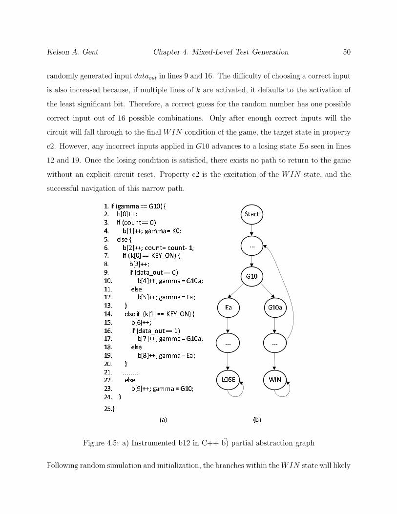
Kelson A. Gent Chapter 4. Mixed-Level Test Generation 50
randomly generated input dataout in lines 9 and 16. The difficulty of choosing a correct input
is also increased because, if multiple lines of k are activated, it defaults to the activation of
the least significant bit. Therefore, a correct guess for the random number has one possible
correct input out of 16 possible combinations. Only after enough correct inputs will the
circuit will fall through to the final WIN condition of the game, the target state in property
c2. However, any incorrect inputs applied in G10 advances to a losing state Ea seen in lines
12 and 19. Once the losing condition is satisfied, there exists no path to return to the game
without an explicit circuit reset. Property c2 is the excitation of the WIN state, and the
successful navigation of this narrow path.
rs tu vwxyyx zz {r|} ~
�s ��|����
�s tu v�����zz |}
�s ��r���� wxyyxz �|�
�s ���� ~
�s ������� �����z ������ r�
�s tu v��|� zz ������} ~
�s �������
�s tu v�x�x����zz |}
r|s ������� wxyyx z{r|x�
rrs ����
r�s ������� wxyyx z �x�
r�s �
r�s ���� tu v��r� zz ������} ~
r�s �������
r�s tu v�x�x����zz r}
r�s ������� wxyyx z{r|x�
r�s ����
r�s ������� wxyyx z �x�
�|s �
�rs ssssssss
��s ����
��s ������� wxyyx z {r|�
��s �
��s�
sss
��x��
{r|
�x {r|x
ssssss
¡�¢���
vx} v�}
Figure 4.5: a) Instrumented b12 in C++ ⁀b) partial abstraction graph
Following random simulation and initialization, the branches within theWIN state will likely

Kelson A. Gent Chapter 4. Mixed-Level Test Generation 51
still be unexercised. As the swarm discovers new branches, the WIN condition is narrowed
down as a hard to reach or random resistant state. Due to its random resistance, the WIN
condition will eventually be targeted by the swarm under our algorithm, as a large majority
other branches are found more easily. Once an ant targets the WIN condition, it analyzes
the constructed path-activation abstraction, shown in Figure 4.5. From this abstraction, it
is shown that state G10 is a dominator for every path that branches from it, since no edges
from previous states bypass it. Therefore, when an ant targets the WIN condition, G10
will be selected in the pool of critical states. When an ant reaches G10 during its walk,
it values inputs that do not activate the path to Ea because it does not see any potential
paths leading to the WIN state from Ea. Therefore, the ant will stall at G10 and attempt
to generate high quality inputs. If the ant finds an input that advances to the state G10a
(the correct key press), the success gets stored in the set of quality vectors for G10. Then,
when the ant approaches G10 again, it attempts to use the inputs from the set of stored
inputs, which represent previous successful key presses, to activate the edge to G10a. If this
fails to advance the state, random generation is attempted again to find a new successful key
press. Eventually, the swarm will generate a set of useful vectors for G10, so that whenever it
reaches state G10, there is a high probability that a useful vector has already been generated
by the swarm. Eventually, an ant will have gained enough information from the rest of the
simulation to be able to successfully press the correct key at every critical point, guiding it
to the WIN state.
Throughout this process, the algorithm updates the pheromone map and hands the vectors to
the gate-level fault simulator process described in 4.4.4. Once the gate-level fault simulation
is complete and the fitness values are updated, a set of high-fitness vectors are selected for
use in the next round.

Kelson A. Gent Chapter 4. Mixed-Level Test Generation 52
4.4.4 Feedback from Gate-level Fault Simulation
The gate-level fault simulation in our algorithm provides a feedback mechanism for improving
RTL vector generation. During the local search, vectors generated by high-fitness ants are
passed to the gate-level. Each of these vectors are evaluated independently and a log is kept
of the faults detected by each vector as well as a cycle by cycle list of fault activation.
Due to the high cost of gate-level fault simulation compared to RTL behavioral simulation,
only high quality ants are selected to be fault simulated to reduce cost. The selection
probability function for simulation is calculated based on the fitness and length of vectors:
P (Skc ) =
(fitnessprefsim(Skc ))
α × (1c)β
∑
Skj∈sets
(fitnessprefsim(Skj ))
α × (1j)β
(4.1)
where the calculation of the fitness prior to fault simulation is given below in Equation 4.2.
Parameters α and β determine the impact of pheromones and vector length on selection
probability. If α = 0.0, only the vector length is considered, and if β = 0.0 then only
pheromone is considered.
Rare fault activation feeds back into the fitness of RTL level faults for all rounds after the
initial simulation. Since the fault is not detected by the sequence, it does not influence
the ant’s current fitness score. However, we attempt to learn information about the fault
activation in relation to RTL structures.
A rare fault activation is an excitation of an undetected fault that occurs in less than 1%
of all cycles. When a rare activation is seen, the branch activation in that cycle is saved.
After fault simulation, the activations during each activation are compared and branches
that appear in all activations of a fault, f , are established as the set of branches for f .
Additionally, a window of length W of the activation path through the extracted FSM is
saved. This information is saved in two sets, Snecc and Sseq, that store all unique necessary
branch conditions and FSM paths for any detected rare faults.

Kelson A. Gent Chapter 4. Mixed-Level Test Generation 53
This information is used to update the fitness values to select candidates for fault simulation
in the next round. Fitness values are updated as shown in Equations 4.2 and 4.3. Nnecc,
where Nseq is the number of times any necessary branch activations have been seen and the
number of times a stored path through the FSM has been activated. Qnecc and Qseq represent
the corresponding base value for each activation.
fitnessprefsim(Skc ) =
∑
b∈Bkc
1
φb
+ exciteprefsim (4.2)
exciteprefsim = Nnecc ×Qnecc +Nseq ×Qseq (4.3)
Newly detected faults are used to help decide which ants will be passed to the next round
of local search. The fitness function for determining ant fitness is shown in Equation 4.4.
The first half of the fitness function is the sum of the reciprocals of the pheromones on
branches activated within set Bkc in iteration c by ant k. The second half of the equation is
the influence of newly detected faults. Ndet represents the number of of previously detected
faults and Qdet is the base increase proportional to the number of remaining undetected
faults.
fitnesspostfsim(Skc ) =
∑
b∈Bkc
1
φb
+Ndet ×Qdet (4.4)
After fault simulation, all ants selected for the next round of vector generation have their
fault coverage added to the global colony detection list and their vectors are saved.
4.4.5 Pheromone Update
The alarm pheromones are updated in a manner similar to [44] based on the number of
times a branch is activated relative to the vector length. The pheromones are updated in
two phases, reinforcement and evaporation.

Kelson A. Gent Chapter 4. Mixed-Level Test Generation 54
Reinforcement: For each branch in the circuit, the branch trace btracek is recorded and a
certain amount of pheromone will be deposited on that trace as a reinforcement:
∀ b ∈ btracek :
φb(t+ 1) = φb(t) +Nh/Nc ×Q(4.5)
where φb(t) is the amount of pheromone on branch b at time t. Nh is the number of times
that the branch b are traversed in a total Nc cycles simulation. Q is the maximum amount
of pheromone released by one ant on one branches.
Evaporation: For every branch in the database, we perform a process of evaporation on it,
via the following equations:
∀ b ∈ tracek, s.t.b 6∈ Snecc :
φb(t+ 1) = (1− ρ1)× φb(t)(4.6)
∀ b ∈ tracek, s.t.b ∈ Snecc :
φb(t+ 1) = (1− ρ2)× φb(t)(4.7)
where 0 < ρ1 ≤ 1 is the default pheromone evaporation rate and 0 < ρ2 ≤ 1 is the pheromone
evaporation rate for branches highlighted by the fault simulator. The evaporation rates adapt
to the response from the fault simulator. If the fault simulator specifies a necessary branch
for rare fault activation, vectors that highly exercise that branch will be rewarded. However,
such rising alarm pheromones may be counter-productive to detecting the rare fault. To
counter act this phenomenon, we increase the evaporation rate so that ρ1 < ρ2.
4.5 Experimental Results
The proposed algorithm was developed on an Intel Core [email protected] with 8 cores
and 16GB of memory running Ubuntu 12.04. Experiments utilized a single core and were

Kelson A. Gent Chapter 4. Mixed-Level Test Generation 55
Table 4.1: Benchmark Characteristics
benchmark #Lines #Branches #FFs #Gates
b07 92 19 49 434
b10 167 32 17 190
b11 118 32 31 397
b12 105 105 121 1120
b13 379 63 53 363
b14 509 211 245 3709
b15 811 141 447 7379
conducted on a set of non-scan ITC99 circuits to assess their performance relative to prior
works. We compared our results versus high-level test generators Htest [22], HYBRO [73],
PRINCE [25], BEACON [44], as well as gate-level test generator STRATEGATE [58]. Note
that for PRINCE, the time of execution was unavailable. We did not compare with previous
mixed-level test generators, because they only reported results for very small circuits, or the
coverages were significantly lower than those shown. The benchmark characteristics for the
circuits used are shown below in Figure 4.1. For each circuit, the number of lines of Verilog
are given, the number of branches and circuit size(#gates and #FFs). Each benchmark has
an explicit reset input signal. Many of the benchmarks contain hard-to-test and hard-to-
traverse structures, which make them great test cases for sequential test generation.
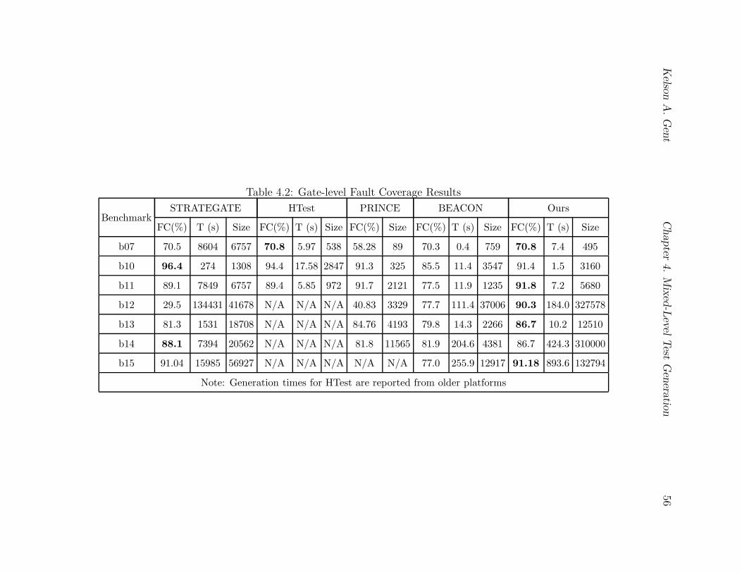
Kelso
nA.Gent
Chapter
4.Mixed-Level
Test
Genera
tion
56
Table 4.2: Gate-level Fault Coverage Results
BenchmarkSTRATEGATE HTest PRINCE BEACON Ours
FC(%) T (s) Size FC(%) T (s) Size FC(%) Size FC(%) T (s) Size FC(%) T (s) Size
b07 70.5 8604 6757 70.8 5.97 538 58.28 89 70.3 0.4 759 70.8 7.4 495
b10 96.4 274 1308 94.4 17.58 2847 91.3 325 85.5 11.4 3547 91.4 1.5 3160
b11 89.1 7849 6757 89.4 5.85 972 91.7 2121 77.5 11.9 1235 91.8 7.2 5680
b12 29.5 134431 41678 N/A N/A N/A 40.83 3329 77.7 111.4 37006 90.3 184.0 327578
b13 81.3 1531 18708 N/A N/A N/A 84.76 4193 79.8 14.3 2266 86.7 10.2 12510
b14 88.1 7394 20562 N/A N/A N/A 81.8 11565 81.9 204.6 4381 86.7 424.3 310000
b15 91.04 15985 56927 N/A N/A N/A N/A N/A 77.0 255.9 12917 91.18 893.6 132794
Note: Generation times for HTest are reported from older platforms

Kelson A. Gent Chapter 4. Mixed-Level Test Generation 57
4.5.1 Algorithmic Settings
Our approach requires the following parameters: the number of ants is set to K = 200. The
maximum number of iterations is set to R = 10 before steady state. For each round of local
search, the length of random vectors Nc are determined according to the circuits size and
number of faults, with a maximum value of 10000. Local search is terminated when no new
branches are discovered for Nr = 5 rounds. Parameters α and β for pheromone and visibility
are set to 1.0 and 0.5, respectively. The initial amount of pheromone was set to 1000 and
the maximum amount of pheromone released by one ant is 10. Pheromone evaporation rate
ρ1 was set to 10% and ρ2 to 20%. Qnecc was set to 0.001, the same as seeing a branch with
the initialization level of pheromones, Qseq = 0.01 and the sequence window, W , is 10 cycles.
The base increase for new fault detection is 0.002, or roughly equivalent to a branch that
has not been seen in 5 search rounds.
4.5.2 Test Set Quality
Our first set of results on gate-level fault coverage is reported in Table 4.2. Note that
for the high-level test generators, we fault-simulated the obtained vectors to obtain the
corresponding fault coverages. As shown, our method is extremely effective for high fault
coverage. For several circuits, including b11 and b12, we reach previously unreached levels
of fault coverage for non-scan techniques. For example, in circuit b12, STRATEGATE
achieves a coverage of 29.5% in more than 1 day of execution. HTest did not report results
for this circuit. PRINCE achieved 40.83% coverage with 3329 vectors (no execution time was
available for PRINCE). BEACON achieved 77.7% fault coverage in 111 seconds with 37006
vectors. Finally, our method achieved 90.3% coverage in just 184 seconds. The systematic
feedback of gate level information enables us to achieve improved fault coverage over methods
that only utilize a high level of line coverage as their primary metric. This is evident when
compared to BEACON, in which a full branch coverage was not sufficient to achieve the
highest gate-level coverage. Additionally, though the vectors in some cases are significantly
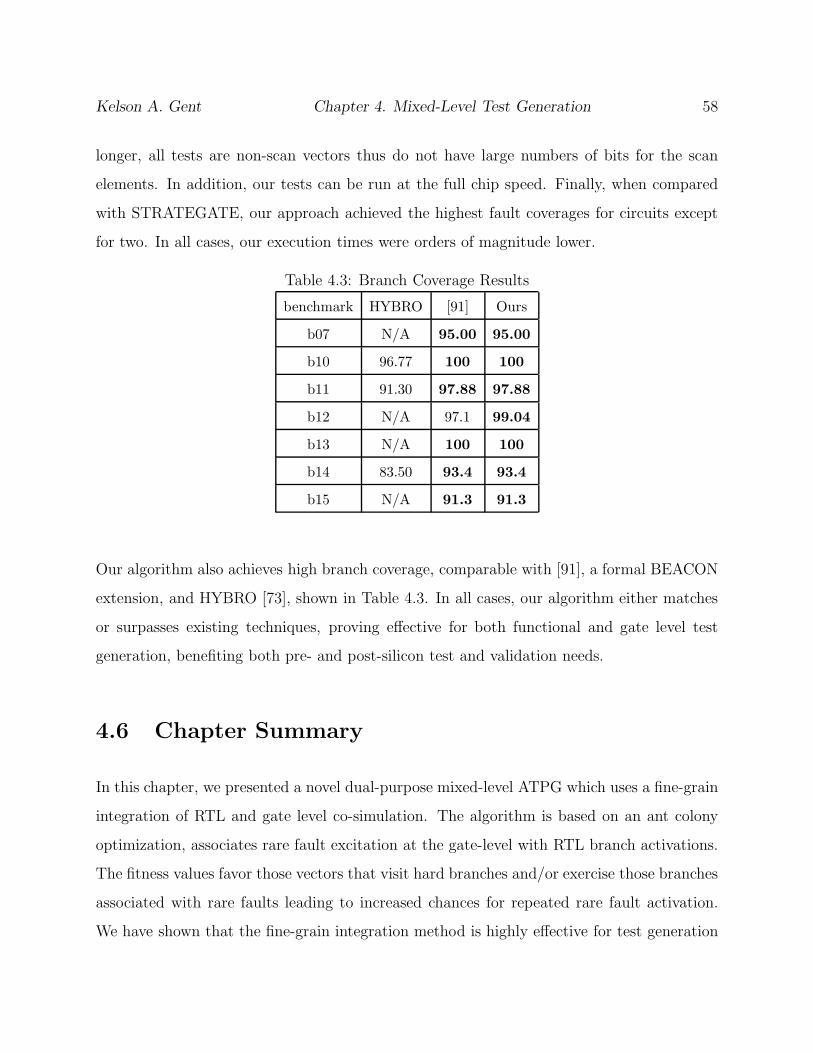
Kelson A. Gent Chapter 4. Mixed-Level Test Generation 58
longer, all tests are non-scan vectors thus do not have large numbers of bits for the scan
elements. In addition, our tests can be run at the full chip speed. Finally, when compared
with STRATEGATE, our approach achieved the highest fault coverages for circuits except
for two. In all cases, our execution times were orders of magnitude lower.
Table 4.3: Branch Coverage Results
benchmark HYBRO [91] Ours
b07 N/A 95.00 95.00
b10 96.77 100 100
b11 91.30 97.88 97.88
b12 N/A 97.1 99.04
b13 N/A 100 100
b14 83.50 93.4 93.4
b15 N/A 91.3 91.3
Our algorithm also achieves high branch coverage, comparable with [91], a formal BEACON
extension, and HYBRO [73], shown in Table 4.3. In all cases, our algorithm either matches
or surpasses existing techniques, proving effective for both functional and gate level test
generation, benefiting both pre- and post-silicon test and validation needs.
4.6 Chapter Summary
In this chapter, we presented a novel dual-purpose mixed-level ATPG which uses a fine-grain
integration of RTL and gate level co-simulation. The algorithm is based on an ant colony
optimization, associates rare fault excitation at the gate-level with RTL branch activations.
The fitness values favor those vectors that visit hard branches and/or exercise those branches
associated with rare faults leading to increased chances for repeated rare fault activation.
We have shown that the fine-grain integration method is highly effective for test generation

Kelson A. Gent Chapter 4. Mixed-Level Test Generation 59
at both the RTL and gate levels, capable of activating deep hard-to-reach branches and
detecting hard-to-test faults without scan, all with low computational costs.

Chapter 5
Abstraction-based Relation Mining
for Functional Test Generation
5.1 Chapter Overview
In this chapter, we present a Register Transfer Level (RTL) abstraction technique to derive
relationships between inputs and path activations. The abstractions are built off of various
program slices. Using such a variety of abstracted RTL models, we attempt to find patterns
in the reduced state and input with their resulting branch activations. These relationships
are then applied to guide stimuli generation in the concrete model. Experimental results
show that this method allows for fast convergence on hard-to-reach states and achieves a
performance increase of up to 9× together with a reduction of test lengths compared to
previous hybrid search techniques.
The rest of the chapter is organized as follows. An introduction is given in Section 5.2.
Section 5.3 describes the methodology of the proposed tool. The experimental results of the
method are given in Section 5.4. Finally, a concluding summary conclude the chapter in
section 5.5.
60
Kelson A. Gent Chapter 5. Relation Mining for Functional Test Generation 61
5.2 Introduction
Functional test generation represents a critical portion of the total effort in modern hardware
designs, in particular for design validation. Due to the high costs associated with design
errors caught during production, ensuring correctness in the design is critical for keeping
costs low while managing the short time-to-market window. As a result, a significant effort
has been invested in automated tools for aiding designers in validation efforts. Generation
of functional tests at the Register Transfer Level (RTL) is a significant step in ensuring the
correctness of the design. Testing at the RTL gives the benefit of automating test generation
at a higher level of design abstraction than at the lower levels. This abstraction level yields
structural information that can be utilized for heuristics to guide the test generation process.
Recently, software metrics have been employed to evaluate the effectiveness of RTL test
generation. A commonly used metric is branch coverage or line coverage [74, 75]. The base
method for generating these tests is random vector generation. Although generation and
application of random test vectors is very fast, these vectors tend to fail to reach corner
cases and states that require a narrow activation path. To counteract this shortcoming,
directed tests are generated to directly reach uncovered corner cases.
Recently, several significant advances have been made in test generation at the RTL utilizing
branch coverage as a metric. HYBRO [73] utilizes a hybrid mechanism that extracts execu-
tion paths from concrete simulation and attempts to reach new branches by mutating these
paths. These mutations are passed to a formal Satisfiability Modulo Theory (SMT) solver as
constraints, which attempts to find inputs that satisfy the mutation. This approach can be
limited due to the computational costs of calling the SMT solver multiple times. Following
HYBRO, BEACON [44] was developed as a purely stochastic method of RTL test gener-
ation utilizing a combination of evolutionary and swarm intelligence techniques. Bounded
model checking was augmented in [91] to help in reaching critical states and trim unreach-
able branches from the search space. Most recently, PACOST [90] utilizes formal methods to
build an onion ring abstraction from the RTL specification for different branch points. This
Kelson A. Gent Chapter 5. Relation Mining for Functional Test Generation 62
abstraction is highly effective for state justification and allows PACOST to quickly reach
difficult corner cases.
We propose a constraint based abstraction for improving branch coverage based test gen-
eration by utilizing mined relations from multiple HDL program slices in order to generate
more effective inputs during runtime. By slicing the HDL, we obtain a reduced model of the
circuit behavior across a few state state variables. Through random simulation of this model,
we may find relationships between state variables, inputs and specific branch activations. By
applying these relationships during test generation, we theorize that our method can reach
high levels of coverage with greater efficiency. While the concept of abstraction is not new
to design validation, we offer the simultaneous use of multiple abstractions to achieve our
goal.
5.3 Methodology
Previous methods in functional test generation rely on distributing the computational load
of navigating corner cases between a deterministic solver and a stochastic search engine.
However, for large circuits, the computation cost associated with a single call to a determin-
istic solver may be significant. Additionally, some conditions may require specific decisions
to be made many cycles before the target condition, which further increases the cost of
of using a deterministic solver and limits the effectiveness of the algorithm. This paper
introduces a method for improving performance of stochastic functional test generation al-
gorithms without the invocation of any formal tools for generating vectors. By utilizing
mined relationships between branch activation and circuit state, our algorithm attempts to
stay in states that dominate the target, applying inputs that were derived during the mining
process. This section describes the proposed abstraction and its integration into the test
generation framework.
Test generation takes place across two stages, a preprocessing and mining stage, and a vector

Kelson A. Gent Chapter 5. Relation Mining for Functional Test Generation 63
generation stage. During the preprocessing stage, program slices are taken of the HDL under
test and are compiled using Verilator and instrumented with a database of counters for branch
coverage. Additionally, the HDL under test is compiled and a mapping is created between
instrumentation points in the sliced circuits and the complete circuit. Then, each slice is
analyzed for relationships corresponding to branch activations. Finally, the concrete circuit’s
CFG is extracted to generate the finite state machine(FSM) for use during test generation.
£¤¥¦ £§¨
©ª«¤¥¬ª®¯
°¥¤¤¬±¤²¬¤ª¥
§¬®
§¬® ³®ª« ´µ¯µ
¶§·¸
¹µ¥µ®¬µ º¬®»µ
¹¼¤¦µ¦ ½µ¾ª®
¹µ¥µ®¬¤ª¥
¿¥¦ºµ®«¤¥¬µÀÁ¿Â쥦 §µ¬®¾Ä
´µ±¬¤ª¥ Å欵
£ª¼¥¦
º¬®»µ ª®
ºÆÀ
Á
Ç
Ç
Figure 5.1: Mining Algorithm Flow
The flow of the test pattern generation is shown in Figure 5.1. At initialization, a set of K
single simulation units, is initialized. Each unit is given an initialization vector to start their
search at a reset condition S0. Following the application of the initialization vector, each unit
simulates a randomly generated vector to eliminate easily reachable branches from target
selection. Next, each search chooses an unreached branch as a target and the dominators
to this node are calculated from the extracted FSM. Once a target is analyzed, stimuli
generation begins and relies on information gained during the mining process to generate
inputs that will advance towards a target state. Vector generation terminates after a unit

Kelson A. Gent Chapter 5. Relation Mining for Functional Test Generation 64
reaches its target branch or after generating a maximum number of vectors, Lmax. Vector
generation terminates when no unit reaches a target forNr rounds or all branches are covered.
The pseudo-code is shown below in Algorithm 5.
Algorithm 5 Test Generation Framework1: extract FSM2: while Suncov 6= ∅ do3: set the initial states to S0
4: countss = 05: set Branchglobalcov = ∅6: for simulation units 1 to K do
7: obtain target, tk8: Branchcov = Scov∪ vector generation(tk, Lmax)9: end for
10: if Scov \ Sglobalcov = ∅ then11: countss++12: increase Lmax
13: else
14: countss = 015: Branchglobalcov = Scov ∪ Branchglobalcov16: end if
17: if countss == Nr then
18: RETURN19: end if
20: end while
5.3.1 Relation Mining
During preprocessing, we generate a set of slices such that each slice satisfies the constraints
of an executable slice as defined by [92]. This implies that for any program point p and a
variable x included in the slice, x will have the same value as in the corresponding program
point p′ of the concrete model. Therefore, relationships and properties mined from the slice
will still hold in concrete model. Each slice is generated based on variables used in control
statements at the RTL. For example, the controlling variable of a switch-case block.
Each slice is compiled using Verilator[76], and randomly simulated from an initialization for

Kelson A. Gent Chapter 5. Relation Mining for Functional Test Generation 65
Nslice cycles by y simulation units. The execution path and circuit state are saved at each
cycle and added to a database. For each unique path within a single cycle, we attempt to
find relations using a template matching system [93]. We have implemented templates for
constant values, variable equality and basic boolean logical operations such as AND, OR,
NOT, etc. For each instance of a particular path, we attempt to match the state to these
templates. Since each template has distinct, distinguishing behavior, this cycle analysis is
used as either a support or counter example to existing relations. Once all cycles have been
processed, the relations are added to a database that can be accessed via their associated
path in the CFG.
The database generated provides a set of constraints for the stochastic search during the
input generation phase of simulation. Each constraint in the database is represented by
the pair (P, f(x)) where P is the single cycle execution path and f(x) is the function of
x that represents the mined constraint. Consider the code and CFG shown in Figure 5.2.
For the path P = 48, 50 (covering coverage points 50 and 48 in lines 2 and 5), we see that
k&0x01 == 1 (k[0] is KEY ON) and data out == 0 must be true to activate the path, which
yields the two relations ({48, 50}, k&1 = 1) and ({48, 50}, data out = 0). The application
of this abstraction in vector generation is described fully in Section 5.3.3.
5.3.2 FSM Extraction
At the RTL, the FSM for the circuit is often explicitly declared. Additionally, each state
in the machine is typically associated with a single branch coverage statement. In order to
associate the branches, we utilize a static analysis method on the CFG extracted by Verilator.
Generally, at the RTL, the FSM is represented by a set of branches controlled by a single
variable which are mutually exclusive within a single cycle. Based the execution of these
branches, the controlling variable will be updated for the next cycle. In order to extract
relationships between these branches, each exclusive branch within the CFG is established
as a node in the FSM and examined for potential assignments to the controlling variable.

Kelson A. Gent Chapter 5. Relation Mining for Functional Test Generation 66
��������������� ������
�������� �������������
�������� �� !"����"�#�$�%��
&������� ����'�"��� "������
������������ ���������&(���
)����������� ��##����*+���
,������� -
(������� �.%��
/������������ ���������&/��
����������� !.�%%�0��1 2����
������������ ��##����* ��
�������� -
����-
��
��
��
ÈÉÊ
Figure 5.2: Relation Example
If an explicit constant assignment to the controlling variable exists, the path is saved as an
edge in the FSM and the new variable is symbolically executed to determine the next states
corresponding branch. Exploring each mutually exclusive path in this manner generates a
representation of the FSM using branch coverage instrumentation points.
Each state in the stored graph is represented by a single branch coverage point s and each
edge is represented as a tuple (scurr, P, snext) where P is a set of branches executed during a
single cycle to transition between scurr and snext.
5.3.3 Vector Generation
Vector generation for each simulation unit is heavily influenced by relations mined during
slice analysis. Compared to previous methods, which walk randomly, our method uses the
relations as generate constrained intelligent inputs that activate branches in the path of the
target branch.
During each simulation units generation, a new input vector is created at each cycle. The

Kelson A. Gent Chapter 5. Relation Mining for Functional Test Generation 67
pseudo-code for this generation is shown below in Algorithm 6. For each unit, an unreached
target branch is passed from the general flow. From this target, tk, the dominator set,
doms(tk), is generated. Following the calculation of dominators, vector generation begins.
At each cycle, based on the execution path in the prior cycle, we calculate the expected state
branch activation in the current cycle, scurr. Then, all relations, R(scurr), whose identifying
path contains scurr are fetched from the database. If there exists any relation in R(scurr)
which defines a relationship based on an input variable, then we attempt to find a matching
state. For each unique path in the relation database that contains branch scurr, the concrete
state is compared to the relations associated with that path. If all relations hold a potential
match is found, the FSM is then queried to determine if snext is also on the dominating path
to the target. If this set of relations leads to another dominating state, then, we apply the
applicable input relations to the generated vector. If not match is found, and there exists
a path in the FSM that leads to a dominating node, then generate an input such that it
does not match any relation with a unique P that yields the same snext. If vector has been
generated that leads to a dominating node, then we generate input randomly because there
is either no node known relation that leads to the target or all possible next states exist
along the path to the target.
Following the generation of a vector, it is simulated and checked for consistency with the
expected results. If our simulated path differs from the result expected based on the given
relation, they are invalidated and removed from the guidance pool, as to not mislead the
algorithm. Additionally, when new branch execution paths are reached, the state is observed
and new potential input relations are identified by passing the inputs into the relation engine.
5.4 Experimental Results

Kelson A. Gent Chapter 5. Relation Mining for Functional Test Generation 68
Algorithm 6 Abstraction Constrained Vector Generation
1: calculate doms(tk)2: for 1 to Nmax do
3: get current state in FSM, scurr4: Gen input = false5: if scurr ∈ doms(tk) then6: Get all relations R(scurr) whose path includes scurr7: if R(scurr) contains input relationships then8: for each unique path, P , in R(scurr) do9: if state variables match relations ∧
P leads to snext | snext ∈ doms(tk) then10: constrain Vconstraint to input relations11: Vsim = Vconstraint12: gen input = true13: end if
14: end for
15: if no matches ∧∃e(scurr, snext) ∈ E(FSM) | snext ∈ doms(tk) then
16: constrain Vconstraint to not match other relations in scurr17: gen input = true18: end if
19: end if
20: end if
21: if ¬gen input then
22: Vsim = Vrand23: end if
24: simulate(Vsim)25: update relations26: end for

Kelson A. Gent Chapter 5. Relation Mining for Functional Test Generation 69
Table 5.1: Relation Mining Benchmark Characteristics
benchmark #Lines #Branches #PIs #POs #FFs
b07 92 19 1 8 49
b10 167 32 11 6 17
b11 118 32 7 6 31
b12 697 105 5 6 121
b12word 877 140 17 18 153
b14 509 211 32 54 245
OR1200-0 943 19 79 111 75
OR1200-1 982 25 144 109 77
OR1200-2 478 19 111 106 4
OR1200-3 579 47 171 230 96
OR1200 26959 684 161 303 2777
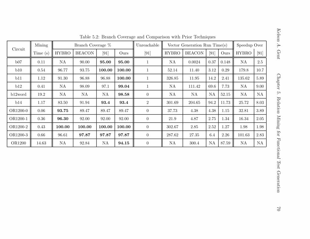
Kelso
nA.Gent
Chapter
5.Rela
tionMiningforFunctio
nalTest
Genera
tion
70Table 5.2: Branch Coverage and Comparison with Prior Techniques
CircuitMining Branch Coverage % Unreachable Vector Generation Run Time(s) Speedup Over
Time (s) HYBRO BEACON [91] Ours [91] HYBRO BEACON [91] Ours HYBRO [91]
b07 0.11 NA 90.00 95.00 95.00 1 NA 0.0024 0.37 0.148 NA 2.5
b10 0.54 96.77 93.75 100.00 100.00 1 52.14 11.40 3.12 0.29 179.8 10.7
b11 1.12 91.30 96.88 96.88 100.00 1 326.85 11.95 14.2 2.41 135.62 5.89
b12 0.41 NA 98.09 97.1 99.04 1 NA 111.42 69.6 7.73 NA 9.00
b12word 19.2 NA NA NA 98.58 0 NA NA NA 52.15 NA NA
b14 1.17 83.50 91.94 93.4 93.4 2 301.69 204.65 94.2 11.73 25.72 8.03
OR1200-0 0.06 93.75 89.47 89.47 89.47 0 37.73 4.38 4.38 1.15 32.81 3.89
OR1200-1 0.36 96.30 92.00 92.00 92.00 0 21.9 4.87 2.75 1.34 16.34 2.05
OR1200-2 0.43 100.00 100.00 100.00 100.00 0 302.67 2.85 2.52 1.27 1.98 1.98
OR1200-3 0.66 96.61 97.87 97.87 97.87 0 287.62 27.35 6.4 2.26 101.63 2.83
OR1200 14.63 NA 92.84 NA 94.15 0 NA 300.4 NA 87.59 NA NA

Kelson A. Gent Chapter 5. Relation Mining for Functional Test Generation 71
The relation mining and targeted ATPG algorithm were developed on an Intel Core i7-
[email protected] with 8 cores and 16GB of memory running Ubuntu 14.04. Experiments
utilized a single core and were conducted on a set of ITC99 [85] circuits to assess their
performance relative to prior works. Additionally, four modules of the OpenRISC1200 [94]
as well as the complete OR1200 circuit are also tested. The four different OR1200 modules
are the instruction cache controller(0), data cache controller(1), Wishbone bus interface(2)
and exception(3). As representatives of general sequential logic, many of the ITC99 [85]
benchmarks circuits have hard-to-reach states (control states), making them a useful case
study for design validation. Additionally, b12word, introduced in [90], is an extension of b12
to expand the search space. B12 is an implementation of a 1 player game where the computer
generates a sequence of numbers and the user must hit the correct button associated with
each generated number, in order, for a sequence of 512 guesses. B12word expands the number
of inputs from 4 to 16, greatly increasing the difficulty of reaching the winning state. The
characteristics of each circuit are shown in Table 5.1, including the number of lines in RTL,
number of branches, number of primary inputs, number of primary outputs, and the number
of flip-flops for each circuit. The complete OR1200 with 2777 state elements is also included
to show that our method is able to process the entire circuit while formal methods will have
difficulty with such a circuit.
5.4.1 Algorithm Settings
The stochastic search algorithm uses the following parameters: the number of simulation
units is set to K = 50. The maximum number of rounds is set to R = 10. For each round
of local search, the length of random vectors Nc is chosen based on the circuit size with a
max vector length of 3000. Local search steady state is assumed after Nr = 5 rounds with
no new branches activated.

Kelson A. Gent Chapter 5. Relation Mining for Functional Test Generation 72
5.4.2 Branch Coverage
Our algorithm maintains the high level of coverage seen in previous works, but at a significant
speedup due to the new feedback techniques employed in this work. The results compared to
HYBRO, BEACON [44], and the technique in [91] are shown in Table 5.2. For each circuit,
the mining time is first reported. Columns 3 to 6 report the branch coverage for HYBRO,
BEACON, [91] and our method, respectively. The known unreachable branches are given in
column 7 and the run time comparison is given in columns 8-11, with speedups reported in
the last two columns. Note that the mining time is short. Most are within 1 second except
for b12word and OR1200, which took under 20 seconds. The initial data mining process is
a one-time cost which does not add much overhead to the final result.
Compared to previous methods, our approach achieves a significant speedup for many bench-
marks. For example, in circuit b11, our method achieves higher coverage than HYBRO,
maintains the same coverage as [91], but it achieves a speedup of 135.62× and 5.89× over
these two techniques, respectively. This speedup comes from two primary factors. First,
the use of purely stochastic methods drastically reduces the computational cost compared
to calls to deterministic solvers on long sequences. Second, the feedback generated by the
proposed path-activation abstraction allows for significantly improved convergence time of
the algorithm compared to previous stochastic methods. This effect is particularly apparent
in circuit b12, which is highly resistant to random stimuli, because following initialization
there are many branches which are uncovered. With our method, those uncovered branches
become explicit targets and vectors are found much more quickly compared to prior ap-
proaches. This convergence factor leads to the 9.00× speedup seen over [91], which was
already considered fast for this challenging circuit. Additionally, We are able to quickly
uncover many branches in the extended circuit b12word providing a high level of coverage
in the case of a significantly expanded input space. In OR1200 with 2777 state elements,
we utilize the mined information from the 4 modules as well as slices taken from OR1200
with ”fsm” and ”ctrl” labels. With our approach, we achieve 94.15% coverage, an improve-

Kelson A. Gent Chapter 5. Relation Mining for Functional Test Generation 73
ment compared to BEACON [44] which achieves a lower 92.84% coverage. Additionally, the
proposed algorithm completes the search in 87.59 seconds, a 3.42× speedup over BEACON.
This improvement comes from significantly higher levels of activation for some FSM states,
which leads to additional coverage of previously unseen conditional branches.
We also report the test vector lengths generated by our algorithm and compare them to
previous works, shown in Table 5.3. [91] does not list vector lengths, so we compare them
to the preceding work, BEACON, and HYBRO. Our algorithm produces quality compact
vectors due to the guidance of the path-activation abstraction. For example, in b10, HYBRO
generated 6450 vectors without reaching 100% coverage, BEACON generated 3547 vectors
that achieved 100% coverage, and the proposed method, which also achieves 100% coverage,
uses only 1973 vectors. By using knowledge about branch activation paths across cycles,
certain conditions are excited earlier in operation leading to the improvements in applied
test length. The notable exception is OR1200, which required more vectors to uncover several
additional hard-to-reach branches.
5.4.3 State Justification
Instead of targeting all branches in the circuit, PACOST [90] is a recent state justification
method also utilizing formal methods for generating vectors to reach a targeted branch
condition. Of particular interest for state justification is the reaching of properties c1 and
c2 for circuit b12, defined by [44]. Unlike PACOST, which targets individual branches, our
method targets all branches. We report the time when the target property is first reached. In
Table 5.4, the minimum-length sequences found by PACOST are compared to our method.
The performance of our method compares favorably to PACOST, despite targeting branch
coverage for the entire circuit. In the case of property c1, our generated sequence is slightly
longer (141 vs. 109) than PACOST, due to the effects of stochastic search and that our
method did not target only property c1. However, this indicates that our abstraction is
effective in guiding the search toward the target without expending many more vectors. Our
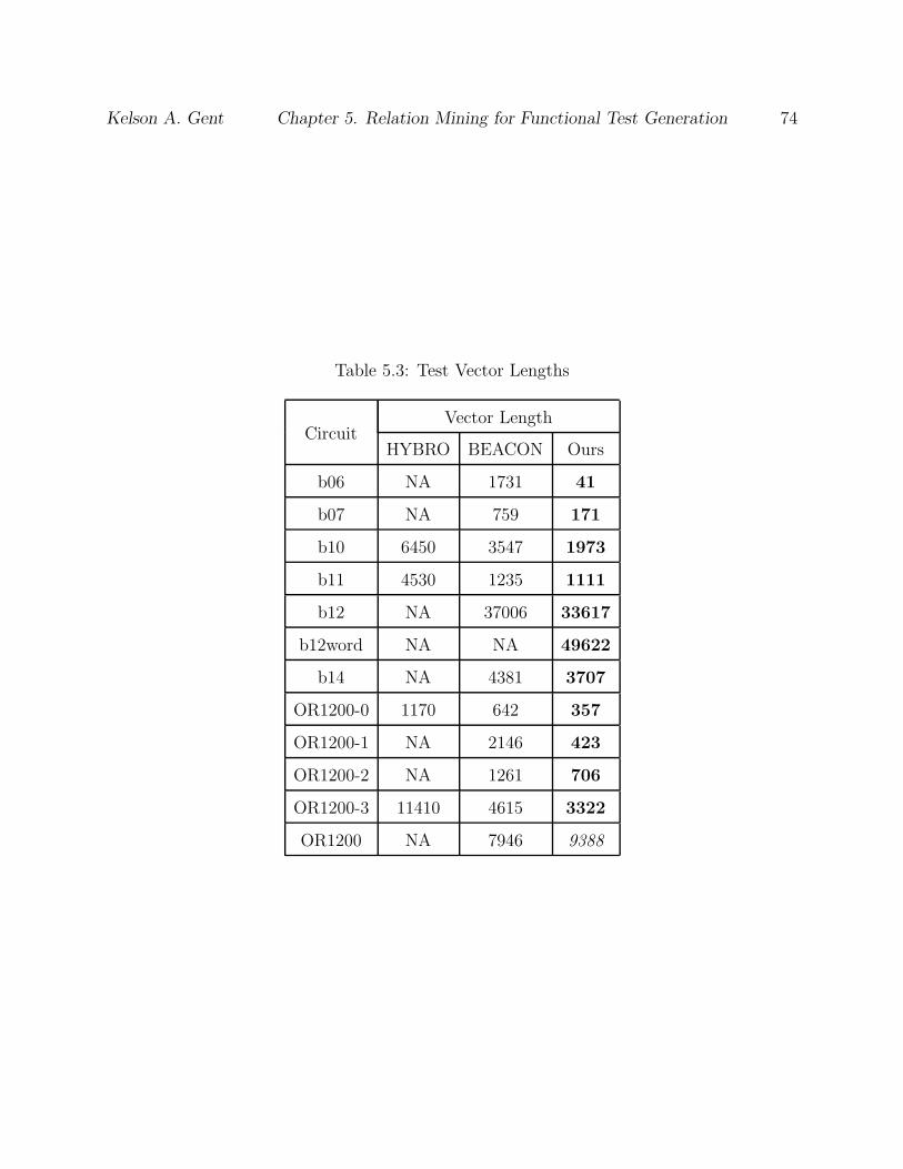
Kelson A. Gent Chapter 5. Relation Mining for Functional Test Generation 74
Table 5.3: Test Vector Lengths
CircuitVector Length
HYBRO BEACON Ours
b06 NA 1731 41
b07 NA 759 171
b10 6450 3547 1973
b11 4530 1235 1111
b12 NA 37006 33617
b12word NA NA 49622
b14 NA 4381 3707
OR1200-0 1170 642 357
OR1200-1 NA 2146 423
OR1200-2 NA 1261 706
OR1200-3 11410 4615 3322
OR1200 NA 7946 9388

Kelson A. Gent Chapter 5. Relation Mining for Functional Test Generation 75
execution time 1.38 seconds, as opposed to 1.87 seconds in PACOST. The performance gain
is likely from the exclusion of expensive formal techniques in our technique. For the more
challenging property c2, our method shows significant improvement over PACOST when
compared to their best reported time. Our sequence is slightly shorter (31900 vs. 33148
vectors). In addition, our method achieves an 11.29× speedup over PACOST even when
we are targeting the circuit as a whole. Additionally, our method is able to justify both
hard-to-reach properties, c1 and c2, in b12word with a relatively low computational effort,
even though PACOST reported results only for c1. These results indicate that the pro-
posed approach is effective at reaching corner states that require traversing through narrow
activation paths. These properties all timed out utilizing the bounded model checker in [91]
Table 5.4: State Justification for b12
PropertyPACOST Ours
length time(s) length time(s)
b12(c1) 109 1.87 141 1.38
b12(c2) 33148 54.22 31900 4.8
b12word(c1) 109 1.92 137 2.1
b12word(c2) N/A N/A 33681 30.86
5.5 Chapter Summary
In this chapter, we presented a novel model for guiding a search for functional test generation
at the RTL. Guidance is provided from relations mined from the simulation of circuit slices
taken from the RTL. This guidance allows us to avoid the invocation of expensive formal
engines to navigate narrow activation paths. This guidance also provides significant boost
to performance showing improvements of up to 9× over previous methods. Additionally,
the algorithm shows the ability to navigate extremely narrow cases such as exercising the

Kelson A. Gent Chapter 5. Relation Mining for Functional Test Generation 76
winning condition in b12word, an expanded version of the b12 circuit, while maintaining
short vector lengths for fast test application

Chapter 6
A Control Path Aware Metric For
Grading Functional Test Vectors
6.1 Chapter Overview
In this chapter, we present a fine-grain behavioral coverage metric for grading functional
test patterns at the RTL. The metric is built using a set of contextual rules for covering
the behavior of each operator. During simulation, the metric is tracked via a set of instru-
mentation points injected during compilation. We show that this metric has a high ranking
correlation value with fault coverage as well as the ability to make reasonable estimations
of fault coverage via a regression based model. Additionally, the metric has a very low
simulation overhead and can be calculated in a single pass of RTL simulation providing sig-
nificant reductions in computational cost compared to other test grading techniques. The
low calculation overhead provides up to two orders of magnitude reduction in execution
time compared to fault simulation and up to an order of magnitude improvement over logic
simulation based fault grading techniques.
The rest of the chapter is organized as follows. Section 6.2 gives a short introduction to
77

Kelson A. Gent Chapter 6. Fault Grading at the RTL 78
prior techniques and our metric. Section 6.3 introduces relevant background topics includ-
ing statistical analysis of time-series data. The metric and it’s application is described in
Section 6.4. Then, Section 6.5 evaluates the efficacy of the methodology on the ITC99 and
OR1200 circuits and provides comparison to previous techniques. These circuits include
several known hard-to-test cases with narrow activation paths, such as b12, as well as a
RISC microprocessor implementation. Finally, Section 6.6 provides a closing summary of
the presented metric.
6.2 Introduction
As circuit design has grown in complexity, traditional methods such as scan-based test are
no longer sufficient to ensure proper behavior in manufactured parts. Complex and transient
defects often require high quality functional test sequences to detect. As a result, design-
for-test (DFT) and design-for-debug (DFD) methods that allow for at-speed application of
vectors, such as logic BIST or Software Based Self Test, have been implemented to aid in
the testing process. Additionally, at-speed testing utilizing functional and application level
test vectors have been used to automate bug detection in modern industrial circuits [95, 96].
However, fault simulating long sequences for large designs can be a bottleneck, since the
computation effort of fault simulating functional vectors at the gate level is significantly
higher. Therefore, fault grading long sequences of functional vectors is critical to ensuring
adequate coverage of defect behaviors. Several fault grading approaches have been proposed
over the years for quickly estimating the fault coverage of a given test vector without the
use of fault simulation.
Simplistic coverage metrics such as net toggle coverage and line coverage at the RTL often
fail to provide adequate prediction of defect coverage in a circuit under test. Therefore, pre-
vious fault grading methods have extensively used fault modeling and statistical sampling
techniques to estimate the overall fault coverage of a test vector [97, 98, 99]. The stratified
Kelson A. Gent Chapter 6. Fault Grading at the RTL 79
sampling method, proposed in [99], estimates the coverage based on a sample of fault ac-
tivity during simulation. The sampled estimation can introduce significant errors when the
fault coverage is low, or when there is a high level of fault activation without propagation.
Additionally, many of these techniques require the pre-calculation of heuristics, such as [98],
that are designed for use on scan or combinational circuits and therefore do not transfer ad-
equately to functional vectors. To address grading of functional vectors, several techniques
have been proposed recently to estimate fault coverage based on gate-level logic simulation
[100, 101]. These techniques use a gate input coverage (GIC) metric and show that the
GIC of a circuit is strongly correlated to fault coverage. This relationship is then used to
create a prediction of fault simulation using partial fault simulation. Several methods have
also been proposed for register transfer level (RTL) fault grading. New coverage metrics are
proposed by [102] which uses a hit count method to estimate coverage and [103] proposes
the use of output deviation, a transition-coverage based method. Additionally, [104] utilizes
an RTL fault model and stratified sampling to build an on the fly estimate of gate level fault
coverage.
The methods for handling functional vectors at the RTL have focused on using predetermined
coverage events defined manually [102] or the statistical estimation of the likelihood of an
output error propagating to an output [103]. Such methods require either significant designer
overhead or are computationally expensive for large circuits. They also require information
from the gate-level to be translated to the RTL to make their estimation, requiring re-
synthesis following every RTL modification. Additionally, many gate level metrics require
special processing to address structures with high controllability that block propagation.
In order to address the aforementioned deficiencies, we propose a new metric for fault grad-
ing at the RTL based on a conjunction of branch coverage and weighted toggle coverage.
Using an RTL observability factor, we weight the new coverage points based on likelihood
of fault propagation. We show that this metric has a high ranking correlation value with
fault coverage as well as the ability to make reasonable estimations of fault coverage via a
regression based model. The metric has a very low simulation overhead and can be done

Kelson A. Gent Chapter 6. Fault Grading at the RTL 80
in a single pass of RTL simulation providing significant reductions in computational cost
compared to other techniques. The metric also provides up to two orders of magnitude
reduction in execution time compared to fault simulation and up to an order of magnitude
improvement over logic simulation based fault grading techniques.
6.3 Background
In this section, we cover necessary statistical background for the regression analysis done in
this work.
6.3.1 Coverage Metrics
Coverage metrics establish a set of discrete points individually associated with a particular
circuit behavior. When the behavior is observed during simulation of a test sequence, the
point is marked as covered. The overall coverage level of a test is expressed as a percentage
of the points covered:
Cov% =#CoveredPoints
#TotalPoints
By calculating the coverage at regular time intervals, we can create a time series of the
coverage during simulation. With each point in the series representing the accumulative
sum of points covered by prior vectors in the test sequence.
6.3.2 Time Series Analysis
When assessing the relationship between different coverage metrics, several factors must be
taken into consideration due to the accumulative nature of the time series. Ordinary least
squares (OLS) and Pearson’s correlation coefficient can sometimes yield spurious correlations
due to the auto-regressive properties of an accumulative sum [105]. An auto-regressive

Kelson A. Gent Chapter 6. Fault Grading at the RTL 81
function is one that is directly related to previous values within the series. In an accumulative
sum, the linear auto-regression takes the form:
Yi = 1.0 · Yi−1 + β + ǫi
The factor of 1.0 on the prior value is referred to as a unit root. This means that our function
has a non-normal distribution and the mean of the series is non-stable. The effect of a unit
root is easily visible in the coverage data for circuit b10 in the ITC99 benchmarks [85] shown
in Figure 6.1. Once an increase in coverage occurs, the coverage value never decreases.
For an example of how an OLS model on raw coverage data can overestimate correlation,
Figure 6.1 shows the b10 coverage data, shown in black, alongside a hypothetical coverage
score represented by the asymptotic logarithmic function, shown in blue:
Log10(1 + x)
1 + Log10(50 + x)
As we can see, for b10, there are two distinct, sharp increases in coverage, at approximately
cycles 1250 and 1900, not represented in the hypothetical model. This means that any
prediction made from the logarithmic model will not represent these events.
However, the least squares correlation coefficient between the two data sets is 0.884 across
the 2000 vectors in the test series leading us to expect a high degree of predictability, at
all points in the time series. In contrast, the corrected model described above shows a
correlation of 0.508 in the rates of change between the two time series. The effect of the
normalization can be seen below in Figure 6.2. The discrepancies are shown as the vertical
line of points near 0 on the X-axis. By using the corrected model, we accurately account for
these types of discrepancies in the model to gauge our prediction confidence.
To remove the unit root, we utilize a first differences or differential model. Given two series
X and Y the first difference model, ∆ is shown below:
∆Yi = Yi − Yi−1
∆Xi = Xi −Xi−1

Kelson A. Gent Chapter 6. Fault Grading at the RTL 82
Figure 6.1: b10 Fault Coverage (black) vs. Predictive Coverage (blue)
In the case of coverage, this translates to the percentage of coverage points detected at a
given time point. However, for coverage data, the mean of the differential model is still
non-stable since the function is asymptotic. To stabilize the differential model, we normalize
using the number of remaining coverage points in the system. The normalization function,
δ, is described by the equation:
δ(Xi) =∆Xi
1.0−Xi−1
In order to make forecasts from the data, we must fit a linear model to the normalized time
series. To do this, a polynomial regression is used since the relationships between the rates
of change may not be perfectly linear. The polynomial regression on the normalized model
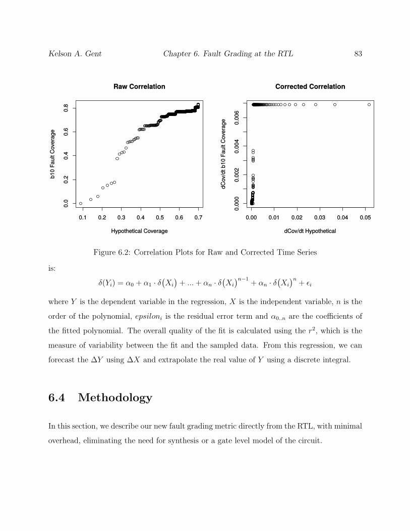
Kelson A. Gent Chapter 6. Fault Grading at the RTL 83
Figure 6.2: Correlation Plots for Raw and Corrected Time Series
is:
δ(Yi) = α0 + α1 · δ(
Xi
)
+ ...+ αn · δ(
Xi
)n−1+ αn · δ
(
Xi
)n+ ǫi
where Y is the dependent variable in the regression, X is the independent variable, n is the
order of the polynomial, epsiloni is the residual error term and α0..n are the coefficients of
the fitted polynomial. The overall quality of the fit is calculated using the r2, which is the
measure of variability between the fit and the sampled data. From this regression, we can
forecast the ∆Y using ∆X and extrapolate the real value of Y using a discrete integral.
6.4 Methodology
In this section, we describe our new fault grading metric directly from the RTL, with minimal
overhead, eliminating the need for synthesis or a gate level model of the circuit.

Kelson A. Gent Chapter 6. Fault Grading at the RTL 84
6.4.1 HDL Preprocessing
We first preprocess the HDL and generate meta-information about the circuit under test to
generate necessary information for our metric. We translate the Verilog circuit description
into a cycle accurate C++ simulation library using Verilator[76], an efficient open source
cross-compiler. During the conversion process, Verilator instruments the HDL with coverage
markers for line coverage. For this work, we extract the control-data flow graph (CDFG) of
the circuit under test and implement a compiler pass to inject a set of monitoring functions
associated with each line coverage point. Additionally, we export each assignment in prefix
notation for the calculation of intermediate values. The preprocessing flow is shown below
in Figure 6.3.
CoverPts.
DPIMonitorInjection
VerilogHDL
VerilatorParse
C++ Simulator
Generation
SymbolTable
MetricSimulator
Figure 6.3: Verilator Compilation with DPI Injection
Assignment monitors are injected as a SystemVerilog Direct Programmable Interface (DPI)[106]
function call in the C++ simulation library. When called, the monitors are passed the current
state of the simulator, their visible scope, and a set of unique identifiers for the assignments
they are monitoring. Then, the DPI function is defined within our coverage code. This plat-
form allows access to the internals of the simulator for the calculation of our metric during
simulation without requiring extensive custom code for each circuit.
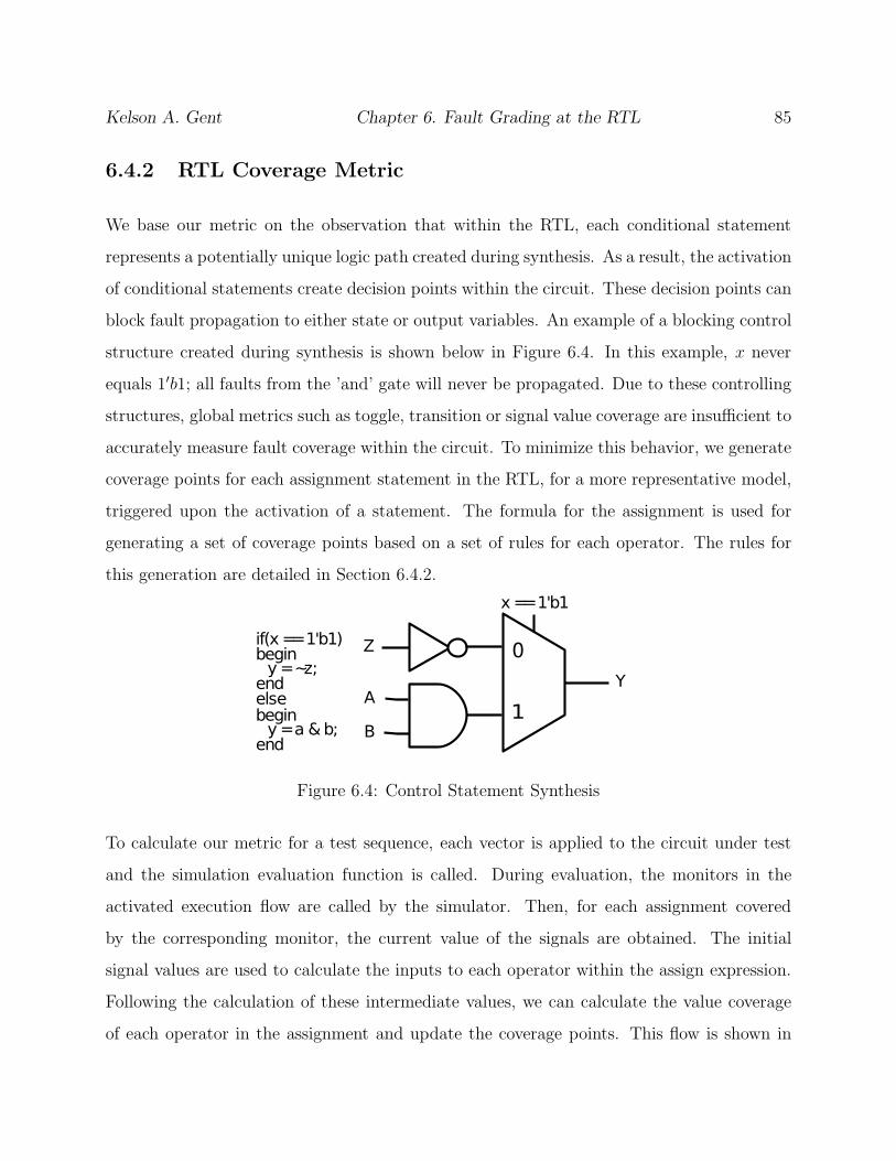
Kelson A. Gent Chapter 6. Fault Grading at the RTL 85
6.4.2 RTL Coverage Metric
We base our metric on the observation that within the RTL, each conditional statement
represents a potentially unique logic path created during synthesis. As a result, the activation
of conditional statements create decision points within the circuit. These decision points can
block fault propagation to either state or output variables. An example of a blocking control
structure created during synthesis is shown below in Figure 6.4. In this example, x never
equals 1′b1; all faults from the ’and’ gate will never be propagated. Due to these controlling
structures, global metrics such as toggle, transition or signal value coverage are insufficient to
accurately measure fault coverage within the circuit. To minimize this behavior, we generate
coverage points for each assignment statement in the RTL, for a more representative model,
triggered upon the activation of a statement. The formula for the assignment is used for
generating a set of coverage points based on a set of rules for each operator. The rules for
this generation are detailed in Section 6.4.2.
if(x == 1'b1)begin
endy = ~z;
elsebegin
endy = a & b;
Y
Z
A
B
x == 1'b1
1
0
Figure 6.4: Control Statement Synthesis
To calculate our metric for a test sequence, each vector is applied to the circuit under test
and the simulation evaluation function is called. During evaluation, the monitors in the
activated execution flow are called by the simulator. Then, for each assignment covered
by the corresponding monitor, the current value of the signals are obtained. The initial
signal values are used to calculate the inputs to each operator within the assign expression.
Following the calculation of these intermediate values, we can calculate the value coverage
of each operator in the assignment and update the coverage points. This flow is shown in
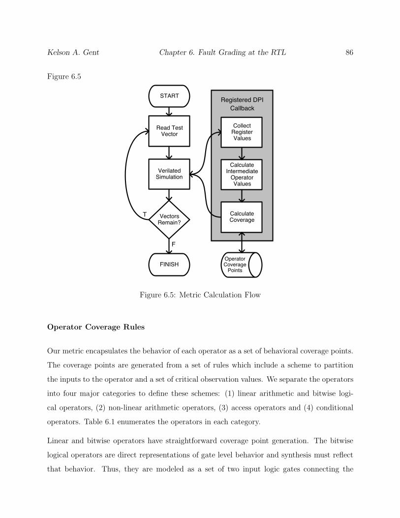
Kelson A. Gent Chapter 6. Fault Grading at the RTL 86
Figure 6.5
Read TestVector
START
OperatorCoverage
Points
F
T VectorsRemain?
VerilatedSimulation
FINISH
CalculateCoverage
CalculateIntermediate
OperatorValues
CollectRegisterValues
Registered DPI
Callback
Figure 6.5: Metric Calculation Flow
Operator Coverage Rules
Our metric encapsulates the behavior of each operator as a set of behavioral coverage points.
The coverage points are generated from a set of rules which include a scheme to partition
the inputs to the operator and a set of critical observation values. We separate the operators
into four major categories to define these schemes: (1) linear arithmetic and bitwise logi-
cal operators, (2) non-linear arithmetic operators, (3) access operators and (4) conditional
operators. Table 6.1 enumerates the operators in each category.
Linear and bitwise operators have straightforward coverage point generation. The bitwise
logical operators are direct representations of gate level behavior and synthesis must reflect
that behavior. Thus, they are modeled as a set of two input logic gates connecting the

Kelson A. Gent Chapter 6. Fault Grading at the RTL 87
Table 6.1: Operator Types
Linear and Bitwise ±,+,−,&, |,∼,∧, >>,<<, reduction
Nonlinear ×,÷,%
Select Operators[]
,[
:]
Conditional Operators ? :
operands. Linear operators are defined as being additive and having a homogeneity of 1 as
shown below.
f(X + Y ) = f(X) + f(Y )
f(τX) = τf(X)
For binary arithmetic, we can represent each operator by partitioning it into bit fields mul-
tiplied by a scalar offset value. For example, a thirty-two bit operand using a partition size
of 8 is represented by X3 · 224 +X2 · 2
16 + X1 · 28 + X0 · 2
0. Due to the additive property,
we can then perform the operation on each partition to obtain the final result. Thus, we
can define the coverage of the arithmetic operator as a behavioral exercization of each cor-
responding pair of bit fields in the operands, represented as {Xpart idx, Ypart idx}. For binary
shift operators, each operation is partitioned into individual bits individually and covered
separately. However, if the digits to be shifted are all one or zero, we do not consider the
shift operand since a single stuck at fault may be undetectable depending on the bit shifted
in. The rules for partitioning and generating coverage points for each linear operator is given
below in Table 6.2.
Non-linear operators are more complicated to properly represent due to the fact that simple
partitioning methods are insufficient to adequately represent the behavior of the operator.
Non-linear operators are typically not additive and we cannot isolate the behavior via a
simple partition across the operator. Therefore, to evaluate non-linear operators, we create
coverage points using an expanded form of the operator.
The expansion for multiplication is based on a technique for self-verifying multipliers [107]
with a low probability of fault escape. In this work, we translate this method into coverage

Kelson A. Gent Chapter 6. Fault Grading at the RTL 88
Table 6.2: Linear Operator Rules
Ops Partition Coverage Values # Cov. Pts.
+,− {Xi, Yi} 00, 01, 10, 11 4 ·min(Wx,Wy)+ |Wx −Wy |
& {Xi, Yi} 11, 01, 10 3 ·min(Wx,Wy)+ |Wx −Wy |
| {Xi, Yi} 00, 01, 10 3 ·min(Wx,Wy)+ |Wx −Wy |
∼ {Xi} 0, 1 2 ·W
∧ {Xi, Yi} 01, 10, 11or00 3 ·min(Wx,Wy)+ |Wx −Wy |
reduction {Xi} 0, 1 2 ·W + 2
>>,<< Xi, Yi 0, 1 & 0, 1 2 ·W + log2(W )
W is the bit width of the operand. X and Y are the operations operands.
points for the multiplication operation. The method utilizes an invariant of multiplication
under modulo arithmetic:
(x modA) · (y modA) ≡ (x · y)(modA)
Using the distributive property of multiplication over addition, we can partition each operand
similarly to the linear operators. An 8-bit operand with 4-bit partitions is represented as
x1 ·24+x0. Thus, an 8 bit multiplication is represented as x ·y = (x1 ·2
4+x0) · (y1 ·24+y0) =
x1y1 ·28+(x1y0+x0y1) ·2
4+x0y0. We then choose a modulus value A such that the partition
offset values always have a value of 1, either 3 or 15 for the 4-bit partition. Applying the
modulo value 3, the multiplication invariant becomes (x · y)mod3 = (x1y1)mod3 + (x1y0 +
x0y1)mod3 + (x0y0)mod3. The modulus values of each of the expanded partitions become
our coverage metric. For this work, we chose a 2-bit partition size with a modulus value of 3.
Each partition combination is calculated and a coverage point is generated for each possible
modulus value.
Access operators, array or bitwise, are a selection from a bit field. Similarly, concatenation
is the creation of a bit field. Concatenation coverage is represented as value coverage of
each input bit. We categorize select into two categories, array select and bit select. For
bit select, we create coverage points for each of the bits in the selection. For array select

Kelson A. Gent Chapter 6. Fault Grading at the RTL 89
operations, we introduce read-validated value coverage points for each bit in the array. These
coverage points are only marked when accessed. To minimize the overhead of our metric
during simulation, we limit the supported memory size to 8192 bits, large enough to handle
most register files.
Conditional operators are a simple coverage system, a single coverage point is created for the
true and false evaluation of the conditional. Following this marking, we only evaluate the
coverage points of the expression that is assigned based on the conditional. In this way, we
automatically account for propagation from the conditional statement. Table 6.3 outlines
the properties of the non-linear, select and conditional operators.
Table 6.3: Non-linear and Access Operator Rules
Ops Partition Values # Cov. Pts.
× mod3 00, 01, 10 3 · (Wx/2 ·Wy/2)
[], [ : ] Xi 0, 1 W
?: cond. true, false 2
Constant reduction allows certain division and modulus operations to be synthesized. Ad-
ditionally, constants change the partitioning schemes for linear operators as some values
become impossible or redundant in the presence of a constant. For division and modulus,
if the constant operand is a power of two, we reduce the operation to a linear shift by a
constant or a bit select. For binary linear operators, only value coverage of the non-constant
operation is considered. Unary operators on constant values are eliminated by the compiler.
Finally, division and modulus operators have many trade-offs between area, frequency, se-
quential versus combinational, and significant power considerations. Due to the large num-
ber of trade-offs involved, many modern synthesis tools do not support variable division and
modulus operators in their synthesizable subset of the HDL. Due to this, we also do not
support variable division or modulus within our metric.

Kelson A. Gent Chapter 6. Fault Grading at the RTL 90
Coverage Point Weighting
The output of logical operations may not correspond to an immediate change of value or
behavioral change within the control path. To adjust for this, we have developed a weighting
scheme for coverage points based on the CDFG extracted during compilation. We estimate
the observability of a register as the graph distance from the output of an assignment to
either an output register or control path register. The observability, W , is then used as a
weighting factor for relative score based on hit count. The formula for the weighted coverage
score is given below:
Cov Score =
hit∑
n=1
( WW−1
)−n
W
Under this scheme, the value of each consecutive coverage point hit decays in value based
on the distance to an output or control variable in the RTL.
6.4.3 Test Quality Analysis
To build our regression model, we simulate test sequences on the RTL model and then fault
simulate the first 25% of the test sequence targeting the single stuck at fault model at the
gate level. Then, we normalize the simulation data as described in Section 6.3 and apply an
exponential weighted moving average low-pass filter to remove temporal noise, smoothing
the data. Following these transformations, we sweep from a first to fourth-order polynomial
regression model with the intercept always going through the origin, α0 = 0 to find the best
possible fit, targeting an r2 > 0.95. Since a least squares polynomial fit can be calculated
very quickly, less than 1 second for 100000 points, it does not effect the overall performance
of the metric.
To obtain the fault coverage estimate, we predict the rate of change of fault coverage for the
remaining 75% of the test sequence and use a discrete integral to obtain the final coverage.
This method has the drawback of introducing integral error to the model so we are limited
Kelson A. Gent Chapter 6. Fault Grading at the RTL 91
in how far ahead we can predict, which is why we chose to simulate 25% of the model.
Additionally, we assess the capability of the metric for appraising test sequences without gate
level simulation. To do this analysis, we utilize Kendall’s correlation coefficient to compare a
set of randomly sampled pairs from the vectors applied to each circuit. Kendall’s correlation
coefficient is a non-parametric rank order coefficient given by the formula:
Nc −Nd
(n)(n− 1)/2
Where Nc is the number of concordant pairs where (xi > xj) ∧ (yi > yj). Nd is the number
of discordant pairs such that (xi > xj) ∧ (yi < yj). n = Nc + Nd. Tied pairs, when
(xi == xj) ∨ (yi == yj), are uncounted.
6.5 Experimental Results
We evaluate the efficacy of the metric using the ITC99 benchmarks[85] and the open source
RISC processor, OR1200 [94]. The OR1200 Verilog description is highly configurable and
can be set up for ASIC or FPGA targeted synthesis. The OR1200 configuration for our
experiments includes the central processing unit, integer divider and multiplier, tick timer
and programmable interrupt controller. Other modules are excluded. Details about the RTL
and gate level descriptions of the benchmarks are shown in Table 6.4.
The experiments were run on a machine with an Intel Core i7-3770K and 16 GB of RAM
running Ubuntu 14.10. For each circuit, random sequences of different lengths were gener-
ated. Additional test sequences generated by STRATEGATE[58] and [108] are included to
assess the metric on high coverage vectors and ensure accurate appraisal across a variety of
conditions
Table 6.5 details the results of our regression-based fault prediction compared to RTL Signal
Toggle and our implementation of the GIC metric, described in [100]. Column 1 lists the
circuit under test. Column 2 and 3 contain the method in which the sequence was generated
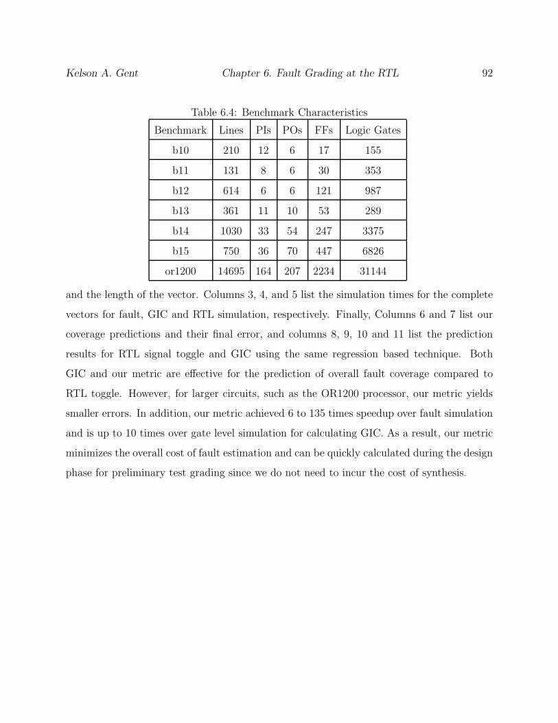
Kelson A. Gent Chapter 6. Fault Grading at the RTL 92
Table 6.4: Benchmark Characteristics
Benchmark Lines PIs POs FFs Logic Gates
b10 210 12 6 17 155
b11 131 8 6 30 353
b12 614 6 6 121 987
b13 361 11 10 53 289
b14 1030 33 54 247 3375
b15 750 36 70 447 6826
or1200 14695 164 207 2234 31144
and the length of the vector. Columns 3, 4, and 5 list the simulation times for the complete
vectors for fault, GIC and RTL simulation, respectively. Finally, Columns 6 and 7 list our
coverage predictions and their final error, and columns 8, 9, 10 and 11 list the prediction
results for RTL signal toggle and GIC using the same regression based technique. Both
GIC and our metric are effective for the prediction of overall fault coverage compared to
RTL toggle. However, for larger circuits, such as the OR1200 processor, our metric yields
smaller errors. In addition, our metric achieved 6 to 135 times speedup over fault simulation
and is up to 10 times over gate level simulation for calculating GIC. As a result, our metric
minimizes the overall cost of fault estimation and can be quickly calculated during the design
phase for preliminary test grading since we do not need to incur the cost of synthesis.
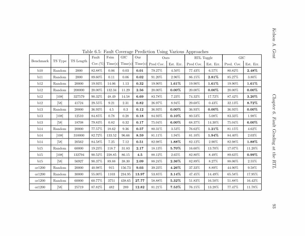
Kelso
nA.Gent
Chapter
6.FaultGradingattheRTL
93
Table 6.5: Fault Coverage Prediction Using Various Approaches
Benchmark TS Type TS LengthFault
Cov.(%)
Fsim
Time(s)
GIC
Time(s)
Our
Time(s)
Ours RTL Toggle GIC
Pred Cov. Est. Err. Pred Cov. Est. Err. Pred. Cov. Est. Err.
b10 Random 2000 82.88% 0.06 0.03 0.01 79.27% 4.50% 77.43% 6.57% 80.82% 2.48%
b11 Random 2000 89.60% 0.11 0.06 0.02 91.20% 2.96% 86.15% 2.81% 85.27% 3.80%
b12 Random 20000 19.93% 14.06 1.13 0.32 19.90% 1.61% 19.90% 1.61% 19.90% 1.61%
b12 Random 200000 20.00% 132.34 11.29 2.56 20.00% 0.00% 20.00% 0.00% 20.00% 0.00%
b12 [108] 327579 90.32% 48.49 14.58 6.69 83.78% 7.23% 74.32% 17.72% 87.42% 3.20%
b12 [58] 41724 29.55% 9.21 2.31 0.82 26.97% 8.94% 29.68% 0.43% 32.13% 8.72%
b13 Random 20000 36.93% 4.5 0.3 0.12 36.93% 0.00% 36.93% 0.00% 36.93% 0.00%
b13 [108] 12510 84.85% 0.78 0.28 0.18 84.93% 0.10% 80.53% 5.08% 83.33% 1.98%
b13 [58] 18708 79.83% 0.82 0.32 0.17 75.04% 6.00% 68.37% 14.30% 75.04% 6.00%
b14 Random 20000 77.57% 18.62 9.36 0.57 80.31% 3.53% 76.62% 1.21% 81.15% 4.62%
b14 [108] 310000 82.72% 133.52 96.66 8.59 81.11% 1.94% 81.10% 1.94% 84.40% 2.03%
b14 [58] 20562 84.58% 7.25 7.12 0.51 82.98% 1.88% 82.12% 2.90% 82.98% 1.88%
b15 Random 60000 19.23% 118.7 31.83 2.17 18.13% 5.70% 16.60% 13.70% 17.07% 11.20%
b15 [108] 132794 90.52% 228.85 86.15 4.5 88.12% 2.65% 82.80% 8.49% 89.63% 0.99%
b15 [58] 56927 90.37% 89.88 38.30 2.09 88.24% 2.36% 82.89% 8.27% 88.06% 2.55%
or1200 Random 20000 40.98% 915 156.73 9.03 39.23% 4.26% 37.33% 8.89% 44.90% 9.58%
or1200 Random 30000 55.00% 1103 234.95 13.97 53.85% 3.14% 47.45% 14.49% 65.58% 17.95%
or1200 Random 60000 60.77% 3751 438.65 27.77 58.88% 5.32% 51.83% 16.50% 51.88% 16.42%
or1200 [58] 25719 87.82% 482 289 12.82 81.21% 7.53% 76.15% 13.28% 77.47% 11.78%

Kelson A. Gent Chapter 6. Fault Grading at the RTL 94
Table 6.6: Kendall Coefficients
Benchmark Ours RTL Toggle GIC
b11 0.972 0.889 .677
b12 0.928 0.064 .570
b13 0.972 0.531 0.862
b14 0.874 0.095 0.936
b15 0.772 0.705 0.754
or1200 0.897 0.799 0.805
Table 6.6 shows the Kendall correlation coefficient from a random sampling of our metric and
fault coverage on vectors applied to each circuit. Results show that our metric typically has
a higher coefficient compared to circuit level toggle and GIC. Since Kendall’s coefficient is
calculated from the number of discordant and concordant pairs, the coefficient is a measure
of agreement between two ranks. Due to the high level of agreement between our metric and
fault coverage, a higher score in our metric likely implies a higher level of fault coverage.
This property allows for the use of our metric as an effective tool in independently ranking
test sequences. In the prior results, only one vector is used for fault prediction for b11,
therefore, we applied two additional random vectors with similar fault coverage and length
to calculate the Kendall correlation. Additionally, in the case of b14, the circuit has many
constant assignments limiting the number of variables available at the RTL compared to the
gate level which reduces the correlation compared to other circuits.
6.6 Chapter Summary
In this chapter, We present a new metric for grading the quality of functional test sequences
at the RTL. The metric can be calculated during a single pass of RTL simulation and rank
correlates strongly with fault coverage on OR1200 and ITC99 benchmarks. The metric
defines rules for each operator and generates coverage points for each assignment in the

Kelson A. Gent Chapter 6. Fault Grading at the RTL 95
circuit description. During simulation, the coverage points calculation is only triggered
when the assignments are executed yielding a metric sensitive to the control state of the
circuit. Experiments show that the metric can be used for making high quality forecasts of
coverage with significantly reduced gate level simulation and provides a strong basis for test
sequence ranking.
Chapter 7
A Framework for Fast ATPG at the
RTL
7.1 Chapter Overview
In this chapter, we present a framework for functional test generation at the RTL. A combi-
nation of static and dynamic analysis is used to seed a meta-heuristic search algorithm. The
search algorithm is implemented as an Ant Colony Optimization using the metric from Chap-
ter 6 as the base heuristic. During the search, ants attempt to target uncovered behavior by
generating inputs from the relationships derived during the seeding analysis. Additionally,
the dynamic analysis is used to track the visibility of the underlying heuristic and ensuring
that propagating behavior is not devalued within the search, even in the absence of the novel
operator behavior. This method allows us to generate high quality coverage test patterns
without any structural circuit information. By leveraging the RTL in this manner, we are
able to achieve similar levels of coverage in orders of magnitude less time than purely gate
level techniques and an order of magnitude faster than the best known mixed level tech-
niques. Additionally, we are able to justify narrow behavioral paths within circuits through
examination of the behavioral information present at the RTL that are unactivated using
96
Kelson A. Gent Chapter 7. Test Pattern Generation at the RTL 97
gate level sequential ATPG tools.
We organize the remainder of the chapter as follows. Section 7.3 presents background in-
formation on time series analysis and necessary statistics. Section 7.4 describes our metric
and its implementation. Section 7.5 presents the efficacy of the methodology on the ITC99
and OR1200 circuits and provides comparison to previous techniques. These circuits in-
clude several known hard-to-test cases with narrow activation paths, such as b12, as well as
a RISC microprocessor implementation. Finally, Section 7.6 provides closing analysis and
future direction.
7.2 Introduction
Due to the growth in circuit complexity, conventional test methodology, such as scan based
testing, is no longer sufficient to ensure proper post-manufacturing behavior. Power aware
testing relies on test patterns that accurately represent realistic operation conditions to
test power conditions. Complex and transient defects may require high-quality at-speed
tests to adequately cover all defects [109]. To address these issues, functional tests are
being used more frequently for testing across the entire design process [96, 95]. However,
high quality functional/sequential automatic test pattern generation (ATPG) is extremely
computationally expensive, particularly for large circuits. To manage this complexity, RTL
ATPG has become a significant area of interest to generate functional test patterns. Test
patterns that simultaneously provide high levels of coverage for RTL verification and at-
speed coverage stand to yield significant savings in the time and monetary costs of test and
verification.
Gate level sequential ATPG techniques, such as [58], have used swarm intelligence and evo-
lutionary techniques to generate vectors. However, for circuits with deep sequential paths,
the lack of guiding information causes these techniques to fail to generate vectors which ad-
equately exercise the circuit. Several prior techniques for generating sequential vectors have
Kelson A. Gent Chapter 7. Test Pattern Generation at the RTL 98
been proposed at the RTL to address these issues. PRINCE [25] and other early RTL-based
method utilize line coverage as their primary coverage metric. However, line coverage sat-
urates significantly earlier than fault coverage and creates gaps in defect coverage. To gain
more accurate information at the RTL [22] represents the RTL as assignment decision dia-
grams to utilize formal techniques for test generation. A hybrid model was proposed in [86]
using a polynomial circuit model to leverage simulation alongside the use of formal models.
However, these techniques frequently fail to reach deep, narrow states due to the significant
overhead imposed by their use of bounded model checking. Recently, significant advances
in RTL state justification have been made utilizing swarm intelligence and hybrid-stochastic
models. BEACON [44], utilized an evolutionary ant colony optimization to generate func-
tional verification vectors targeting branch coverage. PACOST [90] uses a formal model to
generate an onion-ring guidance model for simulation. In [110] a data-mining based approach
to learn about cross cycle transitions which are used to guide the test generation towards
specified target states. However, all these methods utilize macro level coverage techniques,
such as branch coverage, which do not adequately represent low level defects within the
design. To target the gate level from the RTL, mixed level generation is used in [87, 89, 108],
these methods generate vectors at the RTL and then refine the generation process using
information using gate level simulation or test generation. However, the invocation of gate-
level fault simulation requires the generation of a structural model and the invocation of
gate-level simulation significantly slows these methods restricting the gained benefit from
generation at the RTL.
To fully leverage the RTL, a framework for doing functional test pattern generation targeting
defect coverage and functional verification using a combination of static and dynamic analysis
techniques to aid the guidance of a swarm intelligence based test pattern generation engine.
The base coverage metric is built on a bitwise behavioral coverage of each operator present in
the RTL description. A coverage point is generated for each desired input value to properly
exercise the operator. During test generation we attempt to generate vectors that generate
and propagate previously unseen behavioral coverage. By targeting this fine grain behavioral
Kelson A. Gent Chapter 7. Test Pattern Generation at the RTL 99
metric, we can provide vectors with a high level of confidence with regards to defect coverage
and design behavior coverage.
The test generation algorithm described in this chapter is an Ant Colony Optimization
(ACO) meta heuristic using the operator coverage metric as the base heuristic. Initially,
the circuit is compiled to a fast, optimized cycle-accurate C++ model and instrumented
for operator coverage. Additionally, an annotated DDG is extracted and analyzed to learn
predictable relationships between cycles. Then, during test generation, each ant generates
a sequential test vector and simulates using the verilated C++ model. During simulation,
the impact of primary inputs and their effects on the coverage is tracked through the use
of tags, adapted from dynamic taint analysis. Following simulation, A fitness score for each
ant is assessed by the level of operator coverage and behavior propagation provided by the
test vector. Using this as feedback the colony is able to target sections of the code with low
levels of excitation and propagation.
7.3 Background
In this section, we cover dynamic taint analysis and data flow analysis techniques used in
this chapter.
7.3.1 Data Flow Analysis
Data flow analysis is conducted on the CFG of a program. From the CFG, a Data Depen-
dency Graph(DDG) can be generated. The DDG elaborates dependencies between register
assignments, control statements and previously assigned data. Data dependencies are de-
fined as operations which rely upon the data assigned to an operand during a prior operation.
Control dependencies are the dominance frontier of a node in the reverse CFG, representing
the necessary control path required to activate a particular operation. Data dependency

Kelson A. Gent Chapter 7. Test Pattern Generation at the RTL 100
analysis has been used extensively in program scheduling, software change impact analysis
and compiler analysis [111, 112, 113].
Constant propagation is one type of data flow analysis for assessing the impact of a con-
stant assignment. Within the RTL, finite state machines are often defined using constant
assignments. Additionally, switch-case statements and similar are often defined by a set of
constants. In this work, we define a method of analysis to learn about cross cycle behavior
by analyzing the effect of a constant assignment to learn potential behaviors in the next
cycle based on the effects of constants within the RTL.
7.3.2 Dynamic Taint Analysis
Dynamic taint analysis[114] provides a methodology for the analysis of data the derives from
user input within a program. During execution of a program, data is tracked from a data
source to data sink. Any value whose source is directly controllable from user input is tagged
as tainted (T). All other values are marked untainted (F). Then, a policy P is created to
define the flow of taints through the program during execution.
Taints are represented as the tuple 〈v, t〉, where v is a value generated during execution and
t is the taint status of the value. Taint policies show where a taint is used, typically based on
operator semantics, and distinguish between τscalar(scalar value taints) and τmem (Memory
cell taints). Each policy defines three properties for each location: Taint introduction,
taint propagation, and taint checking. Taint introduction defines the conditions when an
operation marks the value as tainted. Taint propagation defines how a taint passes through
an operation to τscalar or τmem. Finally, taint checking determines the safety of the operation
in the presence of a taint. During the analysis if an unsafe operation is executed with a
tainted value, the check is violated and reported as a potential hazard.
Within this work, we use taints to track the effects of behavior propagation within the circuit.
We use the property of a taint representing the observed impact of data during execution
Kelson A. Gent Chapter 7. Test Pattern Generation at the RTL 101
to track the runtime impact of activated behaviors. This property ensures that taints that
never reach observable points are guaranteed to be undetected within the current execution.
7.4 Methodology
In this section, we describe the methodology used for test pattern generation at the RTL in-
cluding, process flow, data analysis techniques and the integration of the analysis techniques
into the swarm intelligence framework
7.4.1 Process Overview
Our methodology utilizes analyses at multiple sections within the test flow to effectively
learn about the design under verification for test pattern generation. The flow of the test
generation framework is illustrated below in Figure Figure 7.1.
Initially, the circuit is compiled using Verilator[76] to generate a cycle-accurate simulation
library in C++. During the compilation process, we do several stages of static analysis.
Initially, instrument the Verilog RTL description for line and operator coverage. Then, a
path-annotated DDG is generated and cross cycle implications are derived to learn static
circuit behavior. The results of the analysis are then passed to the test pattern generation
engine which generates a set of functional test vectors as described in Section 7.4.5.
7.4.2 Operator Coverage
In addition to the operator coverage points defined in [115], we add new coverage points for
conditional operators within branching statements. To generate these coverage points, we
utilize techniques based on domain coverage[116]. The condition is treated as a boundary
between two domains, true and false. Conventional domain testing aims to properly exercise

Kelson A. Gent Chapter 7. Test Pattern Generation at the RTL 102
Figure 7.1: Process Flow
the condition such that tests near the boundary that have a high likelihood of a domain
change in the presence of a defect. We extend this concept to emphasize that domain
changes due to defects do not only occur along the boundary but also at specific ranges
based on the conditions.
For the two different types of logical operators, Boolean arithmetic and numerical compar-
ison, different techniques measure the corresponding coverage. For Boolean operators, the
bitwise counterpart for each single bit is used. To adequately target numerical operators,
a fault on any given bit should cause a behavioral change. Therefore, two conditions must
apply for a bit change to be considered exercised. First, the change must cause the result of
the comparison operator to change value. Second, the change of operator evaluation must
change the evaluation of the entire conditional expression. These two properties ensure that
any defect will cause a behavioral change along the circuit control path. An example is
shown below in Figure 7.2 for the conditional expression X <= 5, when the value of X is

Kelson A. Gent Chapter 7. Test Pattern Generation at the RTL 103
set to 6. Since the binary string for 6 is 0110, the second least significant bit is considered
covered when it is flipped. Note that when the second least significant bit is flipped, X
becomes 0100, or 4, changing the outcome of the conditional X <= 5. A similar analysis
can be performed for the second most significant bit, where 0110 is changed to 0010. In
this case, the result will also alter the outcome of the conditional X <= 5. However, for
covering the least significant bit, a different value for X must be used, since flipping the least
significant bit of 6 (i.e., 0110 to 0111) will not alter the outcome of the conditional.
In our new metric, when all bits of variable involved in a conditional is covered, we guarantee
that a change to any bit position in that variable is captured by at least one test.
X <= 4b'0101
011001000010
Figure 7.2: Bitwise Domain Coverage
For the conditional assignment operator, coverage points are created for just the control
statement, which is sufficient to ensure that each possible assignment has been exercised. A
summary of these additional coverage points is given below in Table 7.1.
Table 7.1: Conditional Operator Overview
Ops Partition Values # Cov. Pts.
∧,∨ X0, Y0 0, 1 4
<,≤, >,≥,=, 6= Xi 0, 1 2 ·Wx + 2 ·Wy

Kelson A. Gent Chapter 7. Test Pattern Generation at the RTL 104
7.4.3 RTL Static Analysis
To aid in guiding input generation, a single-cycle path annotated DDG is generated. This
graph represents the relationships between stored variables from the previous cycle with the
next cycle, as well as inter-cycle dependencies create from combinational logic generated by
blocking assignments. An example of a generated DDG is given below in Figure 7.3.
Figure 7.3: Path Annotated DDG
Following generation, the DDG and CFG are analyzed to learn additional information about
cross cycle behavior within the circuit under test. Within each cycle, there exists a set of
cycle exclusive paths. These paths are formed by conditional structures that only allow for
the activation of a single conditional block at a clock event, such as if-else if chains and
switch-case statements. These structures often define stateful behavior within the circuit,
therefore are a primary target for learning. Using the DDG and single cycle control flow
graph, we generate cross cycle relationships between paths within the RTL. For each variable
that is dependent on a constant assignment, such as stato in Figure 7.3, we apply the value
to dependent conditional statements in the CFG. If the application of the constant causes
a cycle exclusive branch to evaluate to true, we create a relationship between the satisfied
branch and path of the constant assignment in the DDG as well as any necessary constraints
required for the activation. An example of the relations generated from Figure 7.3 is shown
Kelson A. Gent Chapter 7. Test Pattern Generation at the RTL 105
below:
[0]i ∧ (starti+1 = 0)⇒ [1, 2]i+1
[1, 2]i ∧ (starti+1 = 0)⇒ [1, 3]i+1
[1, 3i ∧ (starti+1 = 0)⇒ [1, stato = 20]i+1
7.4.4 RTL Defect Taint Analysis
In circuits with large register files or untestable memory boundaries defect detection by
behavioral coverage metrics often degrades significantly. Large storage structures create
very narrow propagation boundaries where same address reads and writes are required to
propagate the fault out of the memory shadow. Additionally, there are two potential types
of corruption, address and data corruption which further obfuscates defect detection.
To adequately track propagation through large memories, we adapt software dynamic taint
analysis for this work. RTL defect tags represent values during circuit operation that excite
new behavior under operator coverage. We represent these tags as an n-tuple 〈v, cycle, Sbehav〉,
where v is the value that generated the tag, cycle indicates the test cycle in which the value
was generated and Sbehav is a set of operator coverage points carried by the tag.
For propagation of the tags, we define policies for primary inputs, signal assignments, arith-
metic and logical operators, array/memory read/write, and control statements. As in [114],
policies are expressed as boolean expressions that determine the existence of the tag on the
output of the operation. Therefore, generation is denoted as T, propagation based on logical
rules. Additionally, we define further behavior that describes the relationship between a tag,
t and operator coverage. These policies are shown in Table 7.2 below.
The analysis generates tags at three primary points: primary inputs, memory reads at
unwritten addresses and when new operator behavior is exercized without a tag present
on an operand. Tags propagate to different signals via operands. Signals carry a set of
tags, which contain all the behavioral coverage points that have effected that signal. During
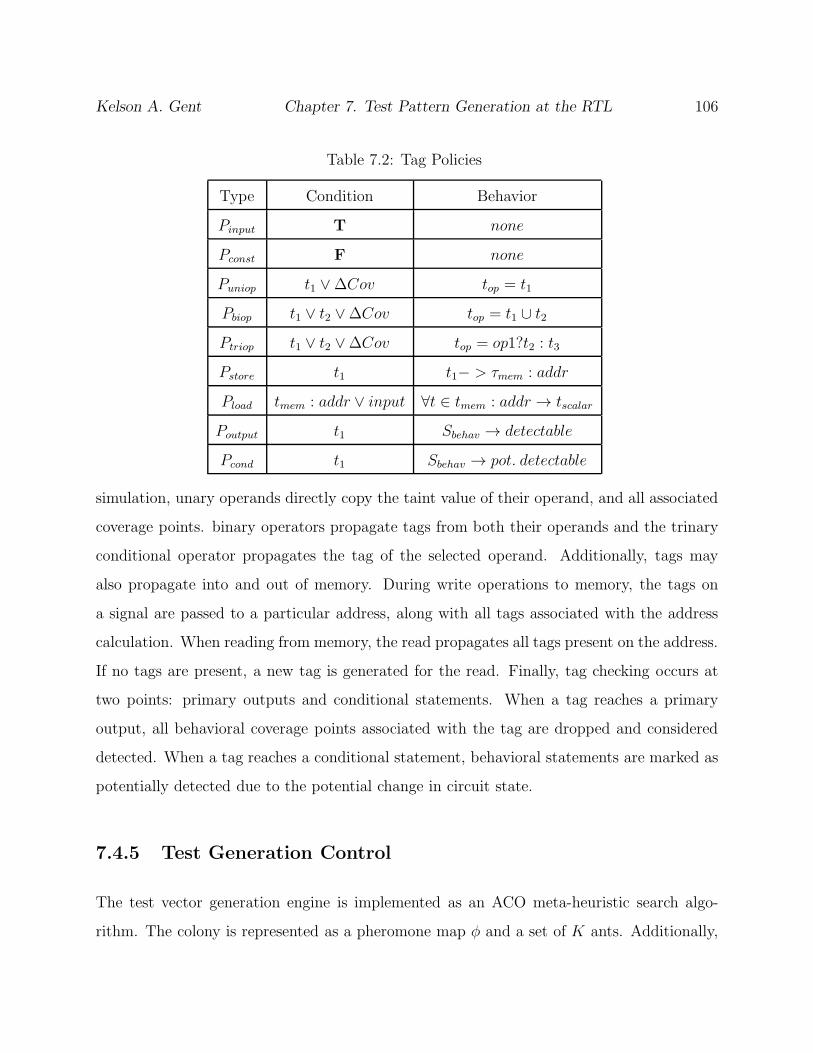
Kelson A. Gent Chapter 7. Test Pattern Generation at the RTL 106
Table 7.2: Tag Policies
Type Condition Behavior
Pinput T none
Pconst F none
Puniop t1 ∨∆Cov top = t1
Pbiop t1 ∨ t2 ∨∆Cov top = t1 ∪ t2
Ptriop t1 ∨ t2 ∨∆Cov top = op1?t2 : t3
Pstore t1 t1− > τmem : addr
Pload tmem : addr ∨ input ∀t ∈ tmem : addr → tscalar
Poutput t1 Sbehav → detectable
Pcond t1 Sbehav → pot. detectable
simulation, unary operands directly copy the taint value of their operand, and all associated
coverage points. binary operators propagate tags from both their operands and the trinary
conditional operator propagates the tag of the selected operand. Additionally, tags may
also propagate into and out of memory. During write operations to memory, the tags on
a signal are passed to a particular address, along with all tags associated with the address
calculation. When reading from memory, the read propagates all tags present on the address.
If no tags are present, a new tag is generated for the read. Finally, tag checking occurs at
two points: primary outputs and conditional statements. When a tag reaches a primary
output, all behavioral coverage points associated with the tag are dropped and considered
detected. When a tag reaches a conditional statement, behavioral statements are marked as
potentially detected due to the potential change in circuit state.
7.4.5 Test Generation Control
The test vector generation engine is implemented as an ACO meta-heuristic search algo-
rithm. The colony is represented as a pheromone map φ and a set of K ants. Additionally,

Kelson A. Gent Chapter 7. Test Pattern Generation at the RTL 107
the colony contains the relationships learned from static analysis, the DDG and statement
information for the calculation of operator coverage. Each ant in the swarm is represented by
an associated test vector and a Verilated C++ simulator instance instrumented for branch
and operator coverage. During the search, each ant in the colony generates vectors from a
starting state S0 according to the relationships derived from static analysis and the current
pheromone map, targeting code blocks with low levels of operator coverage. Then, tags are
generated for the primary inputs and the circuit is simulated. During simulation, operator
coverage are calculated and the tags are propagated based on their policy rules. Each ant
generates and simulates a set number of vectors, Nc, and aggregates the results of the sim-
ulation. Following each ant generation, the generated vector is graded based on the amount
of new operator behavior coverage generated and the amount of behavior propagated to
outputs via tags. Once all ants have been simulated, the colony updates the pheromone map
based on the results of ant simulation and a new round begins by mutating inputs in the
vectors that yielded no new behavior or low tag propagation. This process continues until
no new behavior is propagated to output within a fixed number of rounds Nsteadystate and the
system is assumed to have reached steady state coverage within Nc cycles. Then, if there are
still coverage points left, Nc is increased, expanding the possible search space. This process
continues until an expansion no longer yields new behavior or time out is reached. The flow
of the top level ATPG process is shown below in Figure 7.4.
7.4.6 Ant Vector Generation
During ant simulation, each ant searches from the colony by generating vectors starting from
an initial state S0. Then, each ant generates an initially random test vector of length Nc.
At each cycle, the ant uses the prior execution path and the associated relations to generate
circuit input. First, based on the predicted state from the last cycle, the ant analyzes possible
available subpaths by applying the current circuit state to the relations generated from the
prior state. Each valid sub-path is then graded by the amount of pheromones present along

Kelson A. Gent Chapter 7. Test Pattern Generation at the RTL 108
Initial Random
Sim
Start
End
Init Colony
Start Ants from
S0
Ant Vector
GenerationUpdate
Done?Expand Search
Mutate VectorsSteady
State?
Figure 7.4: Algorithm Flow
the path, preferring the activation of sub-paths that have lower levels of pheromones. Then,
if any of the relations for preferred sub-paths are based on controllable primary inputs, the
constraints are applied directly to the generated inputs. For instance, in Figure 7.3 and the
calculated relations, if start was a primary input then the ant would constrain the value to 0 if
the subpaths 1,2 or 1,3 have lower levels of pheromone than path 0. Following the application
of the constraings, the input is applied and the vector is simulated. During simulation, We
propagate tags based on the observed RTL behavior and the policy rules described in section
7.4.4. Finally, the next state is predicted based on the behavior observed during execution
of the cycle and the relations generated from the annotated DDG. This process continues
until a test pattern of length Nc is generated.
Following the input generation and simulation by each ant, the pheromone map is updated
and the test vector is checked for unique behavioral activations. The vector is mutated at
cycles where the input caused low levels of tag behavior within the circuit. Mutation of low
value test vectors allows for additional potential behavior to be observed while attempting

Kelson A. Gent Chapter 7. Test Pattern Generation at the RTL 109
to maintain the vectors that are necessary for the currently observed behavior. The vector
generation process then restarts and continues until new behavior has not been found for
Nsteadystate iterations. The pseudo-code for this process is shown in Algorithm 7.
Algorithm 7 Ant Search
1: while n < Nsteadystate do
2: for all ants k = 1 to K do
3: for all cycles c = 1 to Nc do
4: analyze sub paths()5: generate constrained input()6: evaluate()7: propagate tags()8: predict next state()9: end for
10: end for
11: update pheromone()12: if new blocks covered then
13: n = 0 { clear the rounds counter}14: else
15: ++n16: end if
17: mutate vector()18: end while
7.4.7 Pheromone Update
Pheromones are laid on code blocks instrumented with operator coverage points. In this
work, Pheromones guide input generation by devaluing input patterns which consistently
activate highly activated code regions during simulation based on tag performance. The
pheromone process happens in two phases reinforcement and evaporation described in the
following subsections.

Kelson A. Gent Chapter 7. Test Pattern Generation at the RTL 110
Reinforcement
Reinforcement highlights areas of highly explored behavior and warns other ants that contin-
ued activation of this behavior is undesirable for test generation. Reinforcement is relative
to the level of coverage and propagation of behavioral coverage points within a code block.
Each level of propagation, potentially detectable, detectable and undetectable, is associated
with a base level of pheromone deposit, Q. The overall amount of pheromones deposited are
weighted based on two factors: Number of uncovered behaviors and the proportion of cov-
erage points in each level of propagation. Additionally, the pheromones added are weighted
based on the number of remaining unactivated behaviors. By doing this, we prevent a
highly activated behavior from devaluing a code block with low levels of overall coverage.
The formula for reinforcing the pheromone map based on execution is given below:
∀b ∈ tracek :
φb(t+ 1) = φb(t) +Qd ·Nd +Qpd ·Npd +Qa ·Na
Npts
Where, Qd, Qpd, Qa is the deposit level of detectable behaviors, potentially detectable and
active but undetectable behaviors, respectively. Nd, Npd, Na are the quantity of each type of
point, and Npts is the total number of points in the associated code block.
Evaporation
Evaporation occurs at two rates based on the propagation of tags to primary outputs. If
a behavior has not been propagated then evaporation happens at a higher rate in order
to encourage continued activation of blocks with non-propagated behavior. Evaporation of
highly propagated blocks happens significantly slower in order to continue to discourage

Kelson A. Gent Chapter 7. Test Pattern Generation at the RTL 111
repeat coverage over time. The formula for pheromone update is expressed as:
∀b ∈ tracek :
φb(t + 1) = (1− ρ) ∗ φb(t)
ρ =ρd ·Nd + ρpd ·Npd + ρbase · (Npts −Nd −Npd)
3
Where, ρd, ρpd, ρbase are the evaporation factors for detectable, potentially detectable and
baseline evaporation.
Evaporation allows for the continued exploration of a branch, even if there is a high level
of activation and low propagation on the branch or if there exist hard to excite behaviors
within the code block. By weighting the evaporation factor based on the status of each type
of point, we can ensure that the ant vector generation does not unnecessarily avoid areas
that have many uncovered or undetected points as the result of undue influence by a few
easily detectable behaviors within a block.
7.5 Results
The effectiveness of the proposed method is evaluated against prior methods using the ITC99
benchmarks [85] and the OR1200 system on a chip (SOC)[94].The OpenRisc1200 circuit
is a highly configurable RISC microprocessor with a harvard-style architecture. We have
configured OR1200 SOC to include a power management unit, debug unit, tick timer, and
programmable interrupt controller in addition to the central processing unit. Within the
OR1200 CPU, we include support for division, multiplication and multiplay-and-accumulate
operators, addc and addic instructions, and the ALU rotate instruction. We also use b10-b15
of the ITC99 benchmarks to evaluate the algorithm. To prove the efficacy of the algorithm
in traversing hard to test paths we use b12 and b12word. B12word is an input-extended
version of the b12 sequencing guessing game, introduced in [90] utilizes sixteen buttons
of input instead of four to greatly increase the difficulty of justifying the games winning

Kelson A. Gent Chapter 7. Test Pattern Generation at the RTL 112
condition. Additionally, we evaluate the algorithm on FabScalar [117], a configurable out-
of-order superscalar RISC processor. For this work, we generated a 32-bit integer FabScalar
microprocessor core using a 9 stage pipeline with an instruction width of 2, an ALU with 4
functional units, 96 physical registers, 32 entry issue queue, bimodal branch predictor and
128 entry reorder buffer, and a rename depth of two.
An overview of the base characteristics of each circuit, including Flip-flops, primary inputs
and outputs, total logic gates, number of lines of RTL and stuck-at fault count. are shown
below in Table 7.3.
Table 7.3: OR1200 & ITC99 Core Characteristics
Circuit # Lines PIs POs DFFs Comb. Faults
b10 210 12 6 17 155 514
b11 131 8 6 30 353 1127
b12 614 6 6 121 987 2878
b12word 782 18 18 207 1648 4732
b13 361 11 10 53 289 937
b14 1030 33 54 247 3375 22802
b15 750 36 70 447 6826 20316
OR1200 14695 164 207 2234 31144 83885
Fabscalar 12594 128 120 14266 121825 810067
7.5.1 Experimental Setup
Our experiments were run on a single core of a Intel [email protected] with 16 GB of RAM
running Ubuntu Linux 14.10. The ant colony is initialized with K = 100 ants to allow for
a broad search within the colony. The maximum number of iterations is set to R = 15 and
Nsteadystate is set to 5. Pheromones on the code blocks are initialized to 0 and the maximum
amount of pheromones that can be dropped for detected points is Qd = 100, potentially

Kelson A. Gent Chapter 7. Test Pattern Generation at the RTL 113
detected points release a maximum of Qpd = 30 and undetected but activated points release
a maximum Qa = 10. The evaporation rates are ρd = 0.05, ρpd = 0.1 and ρbase = 0.2.
7.5.2 Test Vector Quality
We compare our methodology against prior sequential ATPG algorithms in Table 7.5. Com-
parisons are made against the gate level sequential ATPG engine STRATEGATE [58], and
two RTL based ATPG [108, 44]. In order to accurately compare, we utilize the stuck-at
coverage obtained by each method on the benchmark circuits. For the stuck-at fault model,
we are able to achieve a high level of coverage closely comparing to or exceeding the gate
level pattern generator. Additionally, this high level of coverage is obtained as much as
10x faster than the fault co-simulation method used in [108] and more than 100x faster
than the generation time required for gate-level ATPG. Finally, our method is able to pro-
vide high quality coverage in the existence of very hard to justify paths such as b12 and
b12word, which gate level sequential ATPG is unable to generate test patterns that reach
the deep conditions and generates low fault coverage as a result. For example, in circuit
b12, STRATEGATE achieved a fault coverage of only 29.5% in more than one full day of
execution, while achieved 90.3% coverage in 184 seconds, BEACON obtained 77.7% in 111
seconds, and our work achieved 90.11% in just 22.8 seconds. BEACON focuses only on the
high level branch coverage, thus its gate-level fault coverage suffers due to the lack of con-
sideration towards fine grain circuit behavior necessary for fault propagation. In contrast,
[108] and our approach add considerations to target both branch and low-level coverage, the
results is thus improved. Likewise, in circuit b15, we achieved 90.3% fault coverage in slightly
over one minute, and the coverage is very close to the highest known reported, without using
any gate-level information as in [108]. Finally, in OR1200, we achieved nearly two times
the coverage of the BEACON algorithm, further illustrating that targeting software-based
RTL coverage metrics alone is insufficient to achieve adequate defect coverage during test
generation.
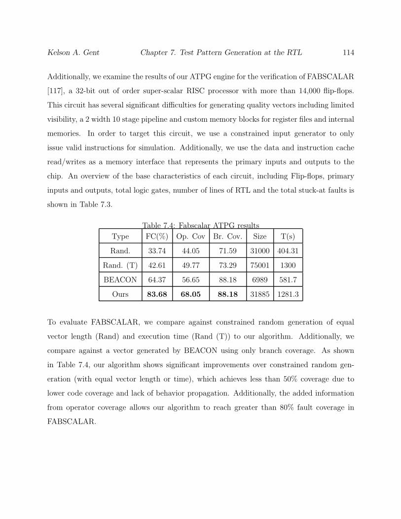
Kelson A. Gent Chapter 7. Test Pattern Generation at the RTL 114
Additionally, we examine the results of our ATPG engine for the verification of FABSCALAR
[117], a 32-bit out of order super-scalar RISC processor with more than 14,000 flip-flops.
This circuit has several significant difficulties for generating quality vectors including limited
visibility, a 2 width 10 stage pipeline and custom memory blocks for register files and internal
memories. In order to target this circuit, we use a constrained input generator to only
issue valid instructions for simulation. Additionally, we use the data and instruction cache
read/writes as a memory interface that represents the primary inputs and outputs to the
chip. An overview of the base characteristics of each circuit, including Flip-flops, primary
inputs and outputs, total logic gates, number of lines of RTL and the total stuck-at faults is
shown in Table 7.3.
Table 7.4: Fabscalar ATPG results
Type FC(%) Op. Cov Br. Cov. Size T(s)
Rand. 33.74 44.05 71.59 31000 404.31
Rand. (T) 42.61 49.77 73.29 75001 1300
BEACON 64.37 56.65 88.18 6989 581.7
Ours 83.68 68.05 88.18 31885 1281.3
To evaluate FABSCALAR, we compare against constrained random generation of equal
vector length (Rand) and execution time (Rand (T)) to our algorithm. Additionally, we
compare against a vector generated by BEACON using only branch coverage. As shown
in Table 7.4, our algorithm shows significant improvements over constrained random gen-
eration (with equal vector length or time), which achieves less than 50% coverage due to
lower code coverage and lack of behavior propagation. Additionally, the added information
from operator coverage allows our algorithm to reach greater than 80% fault coverage in
FABSCALAR.

Kelson A. Gent Chapter 7. Test Pattern Generation at the RTL 115
7.6 Chapter Summary
In this chapter, we describe a test pattern generation engine which directly leverages the
RTL based on the ant colony optimization. By utilizing a combination of static and dynamic
analysis techniques alongside the fine grain operator-based coverage metric from Chapter 6
for estimating behavioral coverage, we are able to guide the test generation engine towards
poorly covered regions, attempting to exercise previously unseen behavior. The guidance
provided yields a test pattern generation engine that can quickly target functional test gen-
eration at the RTL while simultaneously providing a high level of defect test coverage. By
generating test patterns entirely at the RTL, we achieve significant gains in computational
efficiency, gaining a speed up 10× over mixed level techniques and 100× over gate level
techniques in larger circuits as well as being able to target an SOC and circuits with known
hard to reach sequential states.
We additionally show results on a RISC superscalar micro-processor demonstrating func-
tional ATPG capabilities on modern microprocessor architectures.

Kelso
nA.Gent
Chapter
7.Test
Pattern
Genera
tionattheRTL
116
Table 7.5: Sequential Stuck-at Fault Coverage Results
BenchmarkSTRATEGATE [108] BEACON Ours
FC(%) T (s) Size FC(%) T (s) Size FC(%) T (s) Size FC(%) T (s) Size
b10 96.4 274 1308 91.4 1.5 3160 85.5 11.4 3547 91.4 0.51 8344
b11 89.1 7859 6757 91.8 7.2 5680 77.5 11.9 1235 92.54 1.07 20819
b12 29. 5 134431 41678 90.3 184.0 327578 77.7 111.4 37006 90.11 22.8 174382
b12word N/A N/A N/A N/A N/A N/A N/A N/A N/A 86.73 42.76 220556
b14 88.1 1531 20562 86.7 424.3 310000 81.9 204.6 4381 85.7 40.90 176245
b15 91.03 15985 56927 91.18 893.6 132794 77.0 255.9 12917 90.3 70.82 81290
or1200 88.24 18578 25576 N/A N/A N/A 41.4 300.40 7946 81.76 492.68 112369
Note: Generation times for HTest are reported from older platforms
Chapter 8
Conclusion
In this chapter, we summarize the contributions of the dissertation and provide discussion
of future directions of the work.
8.1 Concluding Summary
We have presented two techniques for the utilization of the RTL in test generation. These
techniques spanned two primary areas, functional validation and structural testing. For func-
tional validation, we presented a hybrid approach utilizing an ant colony optimization and
a SMT-based bounded model checker. For structural testing, we introduced an ACO based
system that correlated excited-but-undetected faults with control structures at the RTL in
order to produce high fault coverage test patterns without the use of DFT. Additionally, we
propose three new works for the completion of the dissertation.
In Chapter 3, we presented a hybrid search technique with a limited scope bounded model
checker for design validation in RTL based on branch coverage. To improve performance, we
introduce deterministic methods to help the swarm intelligence algorithm navigate highly
specific execution paths. In order to accomplish this hybridization, we outlined the graph
117
Kelson A. Gent Chapter 8. Conclusion 118
analysis plug-in for Verilator to do the circuit model extraction during compilation. Ad-
ditionally, we described the implementation of our SMT-based BMC. Finally, we proposed
the deterministic search method integration and analyzed the performance of the combined
algorithm. This analysis shows that formal methods can improve the overall coverage of the
algorithm, and in many cases can reduces the overall execution time, due to search space
reduction and faster steady state convergence in the search algorithm.
In Chapter 4, we presented a novel dual-purpose mixed-level ATPG utilizing a fine-grain in-
tegration of RTL and gate level co-simulation. The algorithm associates rare fault excitation
at the gate-level with RTL branch activations through the use of an ACO. The fine-grain
integration method is highly effective for test generation at both the RTL and gate levels,
capable of activating deep hard-to-reach branches and detecting hard-to-test faults without
scan, all with low computational costs. The effectiveness comes from the utilization of a fit-
ness function that rewards the exercization of branches which are shown to excite undetected
faults.
In Chapter 5, we presented a novel model for guiding a search for functional test generation
at the RTL. This guidance mechanism is based on utilizing mined relations from multiple
HDL program slices to control the execution path in the concrete model. The guidance
allows us to avoid the invocation of expensive formal engines to navigate narrow activation
paths. The algorithm yields a significant performance again showing improvements of up
to 9× over previous methods. Additionally, the method yields significantly smaller vector
lengths while maintaining the same level of coverage and is able to justify previous uncovered
states in some benchmarks.
In Chapter 6, a method for grading test patterns at the RTL is presented. The metric utilizes
a a fine-grain operator coverage metric in order to assess how well the pattern exercizes the
behavioral description of the circuit. The metric, calculated entirely at the RTL, shows
high computational efficiency. Speedups compared to gate-level simulation techniques are
upwards of an order of magnitude for GIC and 100× for fault simulation. We then show

Kelson A. Gent Chapter 8. Conclusion 119
that the metric has a high level of rank correlation with stuck-at fault coverage, allowing
for the effective grading of patterns early in the design process. Additionally, we show that
this metric has value during the test cycle by being able to accurately forecast the gate-level
coverage of a pattern from a small initial sampling from gate level fault simulation, greatly
reducing the time necessary to estimate the defect coverage of a pattern.
8.2 Future Work
Through the course of this work, we have shown that the application of software testing tech-
niques and heuristic algorithms have provided significant benefit for sequential and functional
test generation at the RTL. However, analysis techniques for the RTL still lag significantly
behind the techniques available for software analysis. In order to bridge the gap, we present
several potential avenues of future work and their application to the RTL.
First, there is significant opportunity in static analysis of the RTL. Using Verilator, we have
access to the internals of the compilation process. Currently, we use constant propagation
analysis and control-data flow analysis to attempt to seed the ant colony with critical in-
formation. However, this process is limited with regards to the amount of information that
can be derived. Additional analysis techniques that provides input timing information and
further constrains the inputs being generated may provide continued advancement in test
quality and the capability of swarm intelligence based algorithms to justify particular states.
Additionally, Static analysis may help isolate portions of the circuit for large designs, so that
vectors can be generated targeting each portion independently. This is of particular impor-
tance for large modern designs that cannot easily fit into a single workstation’s memory.
Second, the application of additional dynamic analysis techniques may help navigate par-
ticularly difficult structures within the RTL. Illuminating the memory shadow remains a
core difficulty in functional test generation and dynamic analysis techniques may aid in
propagating defect behavior through difficult to test structures.

Kelson A. Gent 120
Finally, bug injection techniques such as mutants testing or value corruption may provide
benefit within RTL ATPG for relating the results of functional test generation at the RTL
to gate level implementations. These methods may also provide methods for targeting par-
ticular behaviors and focusing circuit learning techniques, aiding in functional verification of
the designs as well.

Bibliography
[1] G. Moore, “Progress in digital integrated electronics,” in Electron Devices Meeting,
1975 International, vol. 21, pp. 11–13, 1975.
[2] G. R. Case, “Analysis of actual fault mechanisms in cmos logic gates,” in Proc. Design
Automation Conf., DAC ’76, (New York, NY, USA), pp. 265–270, ACM, 1976.
[3] R. L. Wadsack, “Fault modeling and logic simulation of cmos and mos integrated
circuits,” Bell System Technical Journal, vol. 57, no. 5, pp. 1449–1474, 1978.
[4] G. L. Smith, “Model for delay faults based upon paths,” in Proc. Int. Test Conf.,
pp. 342–351, 1985.
[5] M. Sachdev, Defect Oriented Testing for CMOS Analog and Digital Circuits. Norwell,
MA, USA: Kluwer Academic Publishers, 1998.
[6] M. Bushnell and V. Agrawal, Essentials of Electronic Testing for Digital, Memory and
Mixed-Signal VLSI Circuits. Springer Publishing Company, Incorporated, 2013.
[7] E. M. Clarke, Jr., O. Grumberg, and D. A. Peled, Model Checking. Cambridge, MA,
USA: MIT Press, 1999.
[8] “Statistical analysis of floating point flaw: Intel white paper,” 2004. http://www.
intel.com/support/processors/pentium/sb/cs-013005.htm.
121
Kelson A. Gent 122
[9] I. Hamzaoglu and J. H. Patel, “Deterministic test pattern generation techniques for
sequential circuits,” in Proc. Int. Conf. Computer-Aided Design, pp. 538–543, 2000.
[10] T. Niermann and J. H. Patel, “Hitec: a test generation package for sequential circuits,”
in Proc. Design Automation & Test Europe Conf., pp. 214–218, 1991.
[11] M. Sheeran, S. Singh, and G. St̊almarck, “Checking safety properties using induction
and a sat-solver,” in Proc. of the Third International Conference on Formal Methods
in Computer-Aided Design, FMCAD ’00, (London, UK, UK), pp. 108–125, Springer-
Verlag, 2000.
[12] V. Boppana, S. P. Rajan, K. Takayama, and M. Fujita, “Model checking based on
sequential atpg,” in Computer Aided Verification, pp. 418–430, Springer, 1999.
[13] S. A. Cook, “The complexity of theorem-proving procedures,” in Proceedings of the
Third Annual ACM Symposium on Theory of Computing, STOC ’71, (New York, NY,
USA), pp. 151–158, ACM, 1971.
[14] “State justification benchmarks.” http://filebox.vt.edu/users/minli/Web/
state_just.html.
[15] M. S. Hsiao, E. Rudnick, and J. Patel, “Automatic test generation using genetically-
engineered distinguishing sequences,” in VLSI Test Symposium, 1996., Proceedings of
14th, pp. 216–223, Apr 1996.
[16] M. Li, K. Gent, and M. S. Hsiao, “Utilizing gpgpus for design validation with a mod-
ified ant colony optimization,” in High Level Design Validation and Test Workshop
(HLDVT), 2011 IEEE International, pp. 128–135, Nov 2011.
[17] C. H. Yang and D. L. Dill, “Validation with guided search of the state space,” in Proc.
Design Automation Conf., pp. 599–604, 1998.
[18] V. Bertacco, “Distance-guided hybrid verification with GUIDO,” in Proc. Design Au-
tomation & Test Europe Conf., pp. 151–151, Nov. 2006.

Kelson A. Gent 123
[19] K. Nanshi and F. Somenzi, “Guiding simulation with increasingly refined abstract
traces,” in Proc. Design Automation Conf., pp. 737–742, 2006.
[20] G. D. P. Flavio and A. J. Hu, “An effective guidance strategy for abstraction-guided
simulation,” in Proc. Design Automation Conf., pp. 63–68, 2007.
[21] A. Parikh, W. X. Wu, and M. S. Hsiao, “Mining-guided state justification with parti-
tioned navigation tracks,” in Proc. Int. Test Conf., pp. 1–10, Oct. 2007.
[22] L. Zhang, I. Ghosh, and M. Hsiao, “Efficient sequential atpg for functional rtl circuits,”
in Proc. Int. Test Conf., vol. 1, pp. 290–298, Sept 2003.
[23] A. Asghari, S. Motamedi, and S. Attarchi, “Effective rtl method to develop on-line
self-test routine for the processors using the wavelet transform,” in Computer and
Information Science, 2008. ICIS 08. Seventh IEEE/ACIS International Conference
on, pp. 33–38, May 2008.
[24] S. Ravi and N. Jha, “Fast test generation for circuits with rtl and gate-level views,”
in Test Conference, 2001. Proceedings. International, pp. 1068–1077, 2001.
[25] F. Corno, G. Cumani, M. Reorda, and G. Squillero, “Effective techniques for high-level
atpg,” in Proc. Asian Test Symp., pp. 225–230, 2001.
[26] N. Yogi and V. Agrawal, “Spectral rtl test generation for gate-level stuck-at faults,”
in Test Symposium, 2006. ATS ’06. 15th Asian, pp. 83–88, Nov 2006.
[27] F. Allen, “Control flow analysis,” SIGPLAN Not., vol. 5, pp. 1–19, July 1970.
[28] R. Prosser, “Applications of boolean matrices to the analysis of flow diagrams,” in
Eastern Joint IRE-AIEE-ACM Computer Conference, IRE-AIEE-ACM ’59 (Eastern),
(New York, NY, USA), pp. 133–138, ACM, 1959.
[29] K. Cooper, T. Harvey, and K. Kennedy, “A Simple, Fast Dominance Algorithm.”

Kelson A. Gent 124
[30] L. Davis et al., Handbook of genetic algorithms, vol. 115. Van Nostrand Reinhold New
York, 1991.
[31] J. Horn, N. Nafpliotis, and D. E. Goldberg, “A niched pareto genetic algorithm for mul-
tiobjective optimization,” in Evolutionary Computation, 1994. IEEE World Congress
on Computational Intelligence., Proceedings of the First IEEE Conference on, pp. 82–
87, Ieee, 1994.
[32] J. E. Beasley and P. C. Chu, “A genetic algorithm for the set covering problem,”
European Journal of Operational Research, vol. 94, no. 2, pp. 392–404, 1996.
[33] E. M. Rudnick, J. H. Patel, G. S. Greenstein, and T. M. Niermann, “Sequential circuit
test generation in a genetic algorithm framework,” in Proceedings of the 31st annual
Design Automation Conference, pp. 698–704, ACM, 1994.
[34] R. P. Pargas, M. J. Harrold, and R. R. Peck, “Test-data generation using genetic
algorithms,” Software Testing Verification and Reliability, vol. 9, no. 4, pp. 263–282,
1999.
[35] F. Corno, P. Prinetto, M. Rebaudengo, and M. Sonza Reorda, “Gatto: A genetic algo-
rithm for automatic test pattern generation for large synchronous sequential circuits,”
Computer-Aided Design of Integrated Circuits and Systems, IEEE Transactions on,
vol. 15, no. 8, pp. 991–1000, 1996.
[36] B. F. Jones, H.-H. Sthamer, and D. E. Eyres, “Automatic structural testing using
genetic algorithms,” Software Engineering Journal, vol. 11, no. 5, pp. 299–306, 1996.
[37] M. Dorigo, V. Maniezzo, and A. Colorni, “Ant system: Optimization by a colony of
cooperating agents,” IEEE Tran. Systems, Man, and Cybernetics, vol. 26, pp. 29–41,
Feb 1996.

Kelson A. Gent 125
[38] M. Dorigo and L. Gambardella, “Ant colony system: a cooperative learning approach
to the traveling salesman problem,” Evolutionary Computation, IEEE Transactions
on, vol. 1, pp. 53–66, Apr 1997.
[39] T. Stutzle and H. Hoos, “Max-min ant system and local search for the traveling sales-
man problem,” in Evolutionary Computation, 1997., IEEE International Conference
on, pp. 309–314, Apr 1997.
[40] K. M. Sim and W. H. Sun, “Ant colony optimization for routing and load-balancing:
survey and new directions,” Systems, Man and Cybernetics, Part A: Systems and
Humans, IEEE Transactions on, vol. 33, pp. 560–572, Sept 2003.
[41] V. Maniezzo and A. Colorni, “The ant system applied to the quadratic assignment
problem,” Knowledge and Data Engineering, IEEE Transactions on, vol. 11, pp. 769–
778, Sep 1999.
[42] R. Parpinelli, H. Lopes, and A. Freitas, “Data mining with an ant colony optimization
algorithm,” Evolutionary Computation, IEEE Transactions on, vol. 6, pp. 321–332,
Aug 2002.
[43] C. Solnon, “Ants can solve constraint satisfaction problems,” Evolutionary Computa-
tion, IEEE Transactions on, vol. 6, pp. 347–357, Aug 2002.
[44] M. Li, K. Gent, and M. S. Hsiao, “Design validation of rtl circuits using evolutionary
swarm intelligence,” in Proc. Int. Test Conf., 2012.
[45] M. Li and M. Hsiao, “An ant colony optimization technique for abstraction-guided
state justification,” in Proc. Int. Test Conf., pp. 1–10, nov. 2009.
[46] F. De Paula and A. Hu, “An effective guidance strategy for abstraction-guided simula-
tion,” in Design Automation Conference, 2007. DAC ’07. 44th ACM/IEEE, pp. 63–68,
June 2007.

Kelson A. Gent 126
[47] J. Roth, “Diagnosis of automata failures: A calculus and a method,” IBM Journal of
Research and Development, vol. 10, pp. 278–291, July 1966.
[48] P. Goel, “An implicit enumeration algorithm to generate tests for combinational logic
circuits,” Computers, IEEE Transactions on, vol. C-30, pp. 215–222, March 1981.
[49] H. Fujiwara and T. Shimono, “On the acceleration of test generation algorithms,”
Computers, IEEE Transactions on, vol. C-32, pp. 1137–1144, Dec 1983.
[50] M. Schulz, E. Trischler, and T. Sarfert, “Socrates: a highly efficient automatic test pat-
tern generation system,” Computer-Aided Design of Integrated Circuits and Systems,
IEEE Transactions on, vol. 7, pp. 126–137, Jan 1988.
[51] J.-S. Chang and C.-S. Lin, “Test set compaction for combinational circuits,” in Test
Symposium, 1992. (ATS ’92), Proceedings., First Asian (Cat. No.TH0458-0), pp. 20–
25, Nov 1992.
[52] I. Hamzaoglu and J. Patel, “Test set compaction algorithms for combinational circuits,”
Computer-Aided Design of Integrated Circuits and Systems, IEEE Transactions on,
vol. 19, pp. 957–963, Aug 2000.
[53] I. Pomeranz, L. Reddy, and S. Reddy, “Compactest: a method to generate compact
test sets for combinational circuits,” Computer-Aided Design of Integrated Circuits and
Systems, IEEE Transactions on, vol. 12, pp. 1040–1049, Jul 1993.
[54] P. Flores, H. Neto, and J. Marques-Silva, “On applying set covering models to test set
compaction,” in VLSI, 1999. Proceedings. Ninth Great Lakes Symposium on, pp. 8–11,
Mar 1999.
[55] S. Kajihara, I. Pomeranz, K. Kinoshita, and S. Reddy, “Cost-effective generation of
minimal test sets for stuck-at faults in combinational logic circuits,” Computer-Aided
Design of Integrated Circuits and Systems, IEEE Transactions on, vol. 14, pp. 1496–
1504, Dec 1995.
Kelson A. Gent 127
[56] S. Reddy, I. Pomeranz, and S. Kajihara, “Compact test sets for high defect coverage,”
Computer-Aided Design of Integrated Circuits and Systems, IEEE Transactions on,
vol. 16, pp. 923–930, Aug 1997.
[57] M. S. Hsiao, E. M. Rudnick, and J. H. Patel, “Fast static compaction algorithms for
sequential circuit test vectors,” IEEE Transactions on Computers, vol. 48, pp. 311–322,
Mar 1999.
[58] M. S. Hsiao, E. M. Rudnick, and J. H. Patel, “Sequential circuit test generation using
dynamic state traversal,” in Proc. European Design & Test Conf., pp. 22–28, 1997.
[59] M. S. Hsiao, E. M. Rudnick, and J. H. Patel, “Dynamic state traversal for sequential
circuit test generation,” ACM Trans. Des. Autom. Electron. Syst., vol. 5, pp. 548–565,
July 2000.
[60] D. Krishnaswamy, M. S. Hsiao, V. Saxena, E. M. Rudnick, J. H. Patel, and P. Banerjee,
“Parallel genetic algorithms for simulation-based sequential circuit test generation,” in
VLSI Design, 1997. Proceedings., Tenth International Conference on, pp. 475–481, Jan
1997.
[61] M. S. Hsiao, E. M. Rudnick, and J. H. Patel, “Automatic test generation using
genetically-engineered distinguishing sequences,” in VLSI Test Symposium, 1996., Pro-
ceedings of 14th, pp. 216–223, Apr 1996.
[62] R. Farah and H. Harmanani, “An ant colony optimization approach for test pattern
generation,” in Electrical and Computer Engineering, 2008. CCECE 2008. Canadian
Conference on, pp. 001397–001402, May 2008.
[63] I. Pomeranz and S. Reddy, “Locstep: a logic simulation based test generation proce-
dure,” in Fault-Tolerant Computing, 1995. FTCS-25. Digest of Papers., Twenty-Fifth
International Symposium on, pp. 110–119, June 1995.

Kelson A. Gent 128
[64] R. Guo, S. Reddy, and I. Pomeranz, “Proptest: a property-based test generator for
synchronous sequential circuits,” IEEE Trans. Computer-Aided Design of Integrated
Circuits & Systems, vol. 22, pp. 1080–1091, Aug 2003.
[65] A. Giani, S. Sheng, M. S. Hsiao, and V. Agrawal, “Efficient spectral techniques for
sequential atpg,” in Proc. Design Automation & Test Europe Conf., pp. 204–208, 2001.
[66] S. Sheng and M. S. Hsiao, “Success-driven learning in atpg for preimage computation,”
IEEE Design and Test of Computers, vol. 21, no. 6, pp. 504–512, 2004.
[67] S. Sheng and M. S. Hsiao, “Efficient preimage computation using a novel success-driven
atpg,” in Design, Automation and Test in Europe Conference and Exhibition, 2003,
pp. 822–827, 2003.
[68] M. Banga, M. Chandrasekar, L. Fang, and M. S. Hsiao, “Guided test generation for
isolation and detection of embedded trojans in ics,” in Proceedings of the 18th ACM
Great Lakes Symposium on VLSI, GLSVLSI ’08, (New York, NY, USA), pp. 363–366,
ACM, 2008.
[69] M. Banga and M. S. Hsiao, “A novel sustained vector technique for the detection of
hardware trojans,” in 2009 22nd International Conference on VLSI Design, pp. 327–
332, Jan 2009.
[70] M. Banga and M. S. Hsiao, “Trusted rtl: Trojan detection methodology in pre-silicon
designs,” in Hardware-Oriented Security and Trust (HOST), 2010 IEEE International
Symposium on, pp. 56–59, June 2010.
[71] M. Banga and M. S. Hsiao, “Odette: A non-scan design-for-test methodology for
trojan detection in ics,” in Hardware-Oriented Security and Trust (HOST), 2011 IEEE
International Symposium on, pp. 18–23, June 2011.
Kelson A. Gent 129
[72] B. Alizadeh and M. Fujita, “Guided gate-level atpg for sequential circuits using a high-
level test generation approach,” in Proc. Design Automation Conf., pp. 425–430, Jan
2010.
[73] L. Liu and S. Vasudevan, “Efficient validation input generation in rtl by hybridized
source code analysis,” in Proc. Design Automation & Test Europe Conf., pp. 1–6,
march 2011.
[74] S. Devadas, A. Ghosh, and K. Keutzer, “An observability-based code coverage metric
for functional simulation,” in Proc. Int. Conf. Computer-Aided Design, pp. 418–425,
1996.
[75] B. Beizer, Software testing techniques (2nd ed.). New York, NY, USA: Van Nostrand
Reinhold Co., 1990.
[76] “Verilator.” http://www.veripool.org/wiki/verilator.
[77] L. Moura and N. Bjrner, “Satisfiability modulo theories: An appetizer,” in Formal
Methods: Foundations and Applications (M. Oliveira and J. Woodcock, eds.), vol. 5902
of Lecture Notes in Computer Science, pp. 23–36, Springer Berlin Heidelberg, 2009.
[78] H. Ganzinger, G. Hagen, R. Nieuwenhuis, A. Oliveras, and C. Tinelli, “Dpll(t): Fast
decision procedures,” in Proc. Int. Conf. Computer-Aided Verification, pp. 175–188,
Springer, 2004.
[79] A. Armando, J. Mantovani, and L. Platania, “Bounded model checking of software
using smt solvers instead of sat solvers,” International Journal on Software Tools for
Technology Transfer, vol. 11, pp. 69–83, 2009.
[80] H. Kim, Efficient smt solving for hardware model checking. PhD thesis, University of
Colorado at Boulder, Boulder, CO, USA, 2010. AAI3433303.
[81] “Microsoft research z3 solver.” http://z3.codeplex.com/.

Kelson A. Gent 130
[82] E. Clarke, A. Biere, R. Raimi, and Y. Zhu, “Bounded model checking using satisfiability
solving,” Form. Methods Syst. Des., vol. 19, pp. 7–34, July 2001.
[83] F. Corno, M. S. Reorda, G. Squillero, A. Manzone, and A. Pincetti, “Automatic test
bench generation for validation of rt-level descriptions: an industrial experience,” in
Proc. Design Automation & Test Europe Conf., pp. 385–389, 2000.
[84] T. Zhang, T. Lv, and X. Li, “An abstraction-guided simulation approach using markov
models for microprocessor verification,” in Proc. Design Automation & Test Europe
Conf., pp. 484–489, 2010.
[85] S. Davidson, “Itc99 benchmark circuits - preliminary results,” in Proc. Int. Symp.
Circuits & Systems, p. 1125, 1999.
[86] M. Mirzaei, M. Tabandeh, B. Alizadeh, and Z. Navabi, “A new approach for automatic
test pattern generation in register transfer level circuits,” IEEE Design & Test, vol. 30,
pp. 49–59, Aug 2013.
[87] M. Reni Krug, M. Soares Lubaszewski, and M. de Souza Moraes, “Improving atpg gate-
level fault coverage by using test vectors generated from behavioral hdl descriptions,”
in Proc. VLSI Test Symp., pp. 314–319, Oct 2006.
[88] E. Rudnick, R. Vietti, A. Ellis, F. Corno, P. Prinetto, and M. Reorda, “Fast sequential
circuit test generation using high-level and gate-level techniques,” in Proc. Design
Automation & Test Europe Conf., pp. 570–576, Feb 1998.
[89] S. Ravi and N. Jha, “Fast test generation for circuits with rtl and gate-level views,”
in Proc. Int. Test Conf., pp. 1068–1077, 2001.
[90] Y. Zhou, T. Wang, T. Lv, H. Li, and X. Li, “Path constraint solving based test
generation for hard-to-reach states,” in Proc. Asian Test Symp., pp. 239–244, Nov
2013.

Kelson A. Gent 131
[91] K. Gent and M. S. Hsiao, “Functional test generation at the rtl using swarm intelligence
and bounded model checking,” in Proc. Asian Test Symp., pp. 233–238, Nov 2013.
[92] E. Clarke, M. Fujita, S. Rajan, T. Reps, S. Shankar, and T. Teitelbaum, “Program
slicing of hardware description languages,” in Correct Hardware Design and Verifica-
tion Methods, vol. 1703 of Lecture Notes in Computer Science, pp. 298–313, Springer
Berlin Heidelberg, 1999.
[93] O. Guzey, Data Mining in Constrained Random Verification. PhD thesis, Santa Bar-
bara, CA, USA, 2008. AAI3319881.
[94] “OpenRISC web page.” http://www.opencores.org.
[95] R. McLaughlin, S. Venkataraman, and C. Lim, “Automated debug of speed path
failures using functional tests,” in VLSI Test Symposium, 2009. VTS ’09. 27th IEEE,
May 2009.
[96] L. Lee, L.-C. Wang, P. Parvathala, and T. Mak, “On silicon-based speed path identi-
fication,” in VLSI Test Symposium, 2005. Proceedings. 23rd IEEE, May 2005.
[97] H. Cui, S. C. Seth, and S. K. Mehta, “Modeling fault coverage of random test patterns,”
Journal of Electronic Testing, vol. 19, no. 3, pp. 271–284, 2003.
[98] M. Nakazawa, S. Nitta, and K. Hirabayashi, “Probabilistic fault grading based on
activation checking and observability analysis,” Journal of Electronic Testing, vol. 1,
no. 3, pp. 235–238, 1990.
[99] C. Constantinescu, “Using multi-stage and stratified sampling for inferring fault-
coverage probabilities,” Reliability, IEEE Transactions on, vol. 44, pp. 632–639, Dec
1995.
[100] S. Mirkhani and J. Abraham, “Fast evaluation of test vector sets using a simulation-
based statistical metric,” in VLSI Test Symposium (VTS), 2014 IEEE 32nd, pp. 1–6,
April 2014.
Kelson A. Gent 132
[101] S. Mirkhani and J. Abraham, “Eagle: A regression model for fault coverage estimation
using a simulation based metric,” in Test Conference (ITC), 2014 IEEE International,
pp. 1–10, Oct 2014.
[102] S. Park, L. Chen, P. Parvathala, S. Patil, and I. Pomeranz, “A functional coverage met-
ric for estimating the gate-level fault coverage of functional tests,” in Test Conference,
2006. ITC ’06. IEEE International, pp. 1–10, Oct 2006.
[103] H. Fang, K. Chakrabarty, A. Jas, S. Patil, and C. Tirumurti, “Functional test-sequence
grading at register-transfer level,” Very Large Scale Integration (VLSI) Systems, IEEE
Transactions on, vol. 20, pp. 1890–1894, Oct 2012.
[104] P. A. Thaker, V. D. Agrawal, and M. E. Zaghloul, “A test evaluation technique for
vlsi circuits using register-transfer level fault modeling,” Computer-Aided Design of
Integrated Circuits and Systems, IEEE Transactions on, vol. 22, pp. 1104–1113, Aug
2003.
[105] J. D. Hamilton, Time series analysis, vol. 2. Princeton university press Princeton,
1994.
[106] “Ieee standard for system verilog- unified hardware design, specification, and verifica-
tion language,” 2005.
[107] M. Yilmaz, D. Hower, S. Ozev, and D. Sorin, “Self-checking and self-diagnosing 32-bit
microprocessor multiplier,” in Test Conference, 2006. ITC ’06. IEEE International,
pp. 1–10, Oct 2006.
[108] K. Gent and M. S. Hsiao, “Dual-purpose mixed-level test generation using swarm
intelligence,” in Test Symposium (ATS), 2014 IEEE 23rd Asian, pp. 230–235, Nov
2014.
Kelson A. Gent 133
[109] E. J. McCluskey and C.-W. Tseng, “Stuck-fault tests vs. actual defects,” in Proceedings
of the 2000 IEEE International Test Conference, ITC ’00, (Washington, DC, USA),
pp. 336–, IEEE Computer Society, 2000.
[110] K. Gent and M. S. Hsiao, “Abstraction-based relation mining for functional test gen-
eration,” in VLSI Test Symposium (VTS), 2015 IEEE 33rd, pp. 1–6, April 2015.
[111] J. L. Hennessy and D. A. Patterson, Computer Architecture: A Quantitative Approach.
San Francisco, CA, USA: Morgan Kaufmann Publishers Inc., 3 ed., 2003.
[112] R. S. Arnold, Software Change Impact Analysis. Los Alamitos, CA, USA: IEEE Com-
puter Society Press, 1996.
[113] K. Kennedy and J. R. Allen, Optimizing Compilers for Modern Architectures: A
Dependence-based Approach. San Francisco, CA, USA: Morgan Kaufmann Publish-
ers Inc., 2002.
[114] E. J. Schwartz, T. Avgerinos, and D. Brumley, “All you ever wanted to know about
dynamic taint analysis and forward symbolic execution (but might have been afraid to
ask),” in Proceedings of the 2010 IEEE Symposium on Security and Privacy, SP ’10,
(Washington, DC, USA), pp. 317–331, IEEE Computer Society, 2010.
[115] K. Gent and M. S. Hsiao, “A control path aware metric for grading functional test
vectors,” in Latin American Test Symposium (LATS), 2016 IEEE 17th, April 2016.
[116] Q. Zhang and I. G. Harris, “A domain coverage metric for the validation of behavioral
vhdl descriptions,” in Test Conference, 2000. Proceedings. International, pp. 302–308,
2000.
[117] N. Choudhary, S. Wadhavkar, T. Shah, H. Mayukh, J. Gandhi, B. Dwiel, S. Navada,
H. Najaf-abadi, and E. Rotenberg, “Fabscalar: Automating superscalar core design,”
IEEE Micro, vol. 32, pp. 48–59, May 2012.