highfrequency: toolkit for the analysis of highfrequency ... · pdf filehighfrequency: toolkit...

Highfrequency:

Toolkit for the analysis of highfrequency financial

data in R.

Kris BoudtVU University Amsterdam,

Lessius and K.U.Leuven

Jonathan CornelissenK.U.Leuven

Scott PayseurUBS Global Asset Management

Abstract

The highfrequency package contains an extensive toolkit for the use of highfrequencyfinancial data in R. It offers functionality to manage, clean and match highfrequencytrades and quotes data. Furthermore, it enables users to: calculate easily various liquid-ity measures, estimate and forecast volatility, and investigate microstructure noise andintraday periodicity.

Keywords: High-frequency data, Liquidity, Quotes, R software, Realized volatility, Trades.

1. General information

The economic value of analyzing high-frequency financial data is now obvious, both in theacademic and financial world. It is the basis of intraday and daily risk monitoring and fore-casting, an input to the portfolio allocation process, and also for high-frequency trading. Forthe efficient use of high-frequency data in financial decision making, the highfrequency pack-age implements state of the art techniques for cleaning and matching for trades and quotes,as well as the calculation and forecasting of liquidity, realized and correlation measures basedon high-frequency data. The highfrequency package is the outcome of a Google summer ofcode project and an improved and updated version of the 2 packages: RTAQ (Cornelissen andBoudt 2012) and realized (Payseur 2008).

Handling high-frequency data can be particularly challenging because of the specific character-istics of the data, as extensively documented in Yan and Zivot (2003). The highfrequency

package offers high-level tools for the analysis of high-frequency data. These tools tacklethree typical challenges of working with high-frequency data. A first specific challenge is theenormous number of observations, that can reach heights of millions observations per stockper day. Secondly, transaction-by-transaction data is by nature irregularly spaced over time.Thirdly, the recorded data often contains errors for various reasons.

The highfrequency package offers a (basic) interface to manage highfrequency trades andquotes data. Furthermore and foremost, it offers easy-to-use tools to clean and aggregate high-frequency data, to calculate liquidity measures and, measure and forecast volatility. The toolsin highfrequency are designed in such a way that they will work with most data input types.The package contains an extensive collection of functions to calculate realized measures, since

2 Highfrequency: Toolkit for the analysis of highfrequency financial data in R.

it arose by merging the package RTAQ (Cornelissen and Boudt 2012) from the TradeAnalyticsproject and the package realized (Payseur 2008).

highfrequency strongly builds on the functionality offered by the xts package (Ryan andUlrich 2009) package. You can use the functionality in the highfrequency package for tradesand quotes objects from the most popular vendors, as long as your objects are stored as xtsobjects.

The highfrequency package is hosted on R-forge and the latest version of the package canbe downloaded through the following command:

install.packages("highfrequency", repos="http://R-Forge.R-project.org")

2. Organizing highfrequency data

Users that have their own system set up to store their highfrequency data as xts objects canskip this section. The functions to calculate liquidity, etc. in the highfrequency package cantake highfrequency data of various data vendors as input: NYSE TAQ, WRDS TAQ, Reuters,Bloomberg, etc. To achieve this flexibility, we rely on the functionality provided by theexcellent quantmod package (Ryan 2011). Additionally, highfrequency provides functionalityto convert raw data from several data providers into xts objects. The latter is discussed andillustrated in this section.

Highfrequency financial data is typically subdivided into two files, containing information onthe trades and quotes respectively. highfrequency can currently parse three types of inputdata into xts objects: (i) ”.txt” files extracted from the NYSE TAQ database, (ii) ”.csv” ”filesextracted from the WRDS database, (iii) ”.asc” files from http://www.tickdata.com. Foreach of these input data types, we briefly discuss how the convert function can be used toconvert the txt/csv/asc files into xts objects (Ryan and Ulrich 2009) that are saved on-diskin the “RData” format. We opt to store the data as xts objects because this type of objectcan be indexed by an indicator of time and date.1

Parsing raw NYSE TAQ data into xts:Suppose the folder ~/raw_data on your drive contains the two folders: ”2008-01-02”and ”2008-01-03”. Suppose these folders each contain the files AAPL_trades.txt and AA_trades.txt

with the daily TAQ data bought from the New York Stock Exchange (NYSE) for the AAPL

and AA stock. The raw data can then easily be converted into on-disk xts objects as follows:

from = "2008-01-02";

to = "2008-01-03";

datasource = "~/raw_data";

datadestination = "~/xts_data";

convert(from, to, datasource, datadestination, trades=TRUE,

quotes=FALSE,ticker=c("AA","AAPL"), dir=TRUE, extension="txt",

header=FALSE,tradecolnames=NULL,quotecolnames=NULL,

format="%Y%m%d %H:%M:%S");

1Examples of the use of xts objects can be found on http://www.quantmod.com/examples/data/.

http://www.tickdata.com

http://www.quantmod.com/examples/data/.

Jonathan Cornelissen, Kris Boudt, Scott Payseur 3

At this point, the folder ~/xts_data will contain two folders named 2008-01-02 and 2008-01-03 containing the files AAPL_trades.RData and AAPL_trades.RData which contain therespective daily trade data. The data can now be loaded with the TAQLoad function (seebelow).

Parsing raw WRDS TAQ data into xts:Suppose the folder ~/raw_data on your drive contains the files IBM_quotes.csv andIBM_trades.csv acquired from Wharton Research Data Service (WRDS).2 Both files containrespectively the trade and quote data for the ”IBM” stock for ”2011-12-01” up to ”2011-12-02”.The data can then easily be converted into on-disk xts objects as follows:

from = "2011-12-01";

to = "2011-12-02";



convert( from=from, to=to, datasource=datasource,

datadestination=datadestination, trades = T, quotes = T,

ticker="IBM", dir = TRUE, extension = "csv",

header = TRUE, tradecolnames = NULL, quotecolnames = NULL,

format="%Y%m%d %H:%M:%S", onefile = TRUE )

Now, the folder ~/xts_data contains two folders, one for each day in the sample, i.e. ”2011-12-01” up to ”2011-12-02”. Each of these folders contains a file named IBM_trades.RData inwhich the trades for that day can be found and a file IBM_quotes.RData in which the quotesfor that day can be found, both saved as xts objects. As a final step, the function TAQLoad

can be used to load the on-disk data into your R workspace. You can for example get thetrades for this sample in your workspace as follows:

> xts_data = TAQLoad( tickers="IBM", from="2011-12-01",

+ to="2011-12-02",trades=F,

+ quotes=TRUE, datasource=datadestination)

> head(xts_data)

SYMBOL EX BID BIDSIZ OFR OFRSIZ MODE

2011-12-01 04:00:00 "IBM" "P" "176.85" "1" "188.00" " 1" "12"

2011-12-01 04:00:17 "IBM" "P" "185.92" "1" "187.74" " 1" "12"

2011-12-01 04:00:18 "IBM" "P" "176.85" "1" "187.74" " 1" "12"

2011-12-01 04:00:25 "IBM" "P" "176.85" "1" "187.73" " 1" "12"

2011-12-01 04:00:26 "IBM" "P" "176.85" "1" "188.00" " 1" "12"

2011-12-01 04:00:26 "IBM" "P" "176.85" "1" "187.74" " 1" "12"

Parsing raw Tickdata.com data into xts:Suppose the folder ~/raw_data on your drive contains the files GLP_quotes.asc andGLP_trades.asc acquired from www.tickdata.com. Both files contain respectively the tradeand quote data for the ”GLP” stock for ”2011-01-11” up to ”2011-03-11”. The data can theneasily be converted into on-disk xts objects as follows:

2http://wrds-web.wharton.upenn.edu/wrds

www.tickdata.com

http://wrds-web.wharton.upenn.edu/wrds


from = "2011-01-11";

to = "2011-03-11";



convert(from=from, to=to, datasource=datasource,

datadestination=datadestination, trades = TRUE,

quotes = TRUE, ticker="GLP", dir = TRUE, format = "%d/%m/%Y %H:%M:%OS",

extension = "tickdatacom", header = TRUE, onefile = TRUE );

At this point, the folder ~/xts_data now contains three folders, one for each day in the sam-ple, i.e. ”2011-01-11”, ”2011-02-11”, ”2011-03-11”. Each of these folders contains a file namedGLP_trades.RData in which the trades for that day can be found and a file GLP_quotes.RDatain which the quotes for that day can be found, both saved as xts object. Notice theformat = '%d/%m/%Y %H:%M:%OS' argument that allows for timestamps more accurate thanseconds, e.g. milliseconds in this case. As a final step, the function TAQLoad can be used toload the on-disk data into your R workspace. You can for example get the trade data for thefirst day of the sample as follows:

> options("digits.secs"=3); #Show milliseconds

> xts_data = TAQLoad(tickers="GLP", from="2011-01-11", to="2011-01-11",

+ trades=T, quotes=F,

+ datasource=datadestination)

> head(xts_data)

SYMBOL EX PRICE SIZE COND CORR G127

2011-01-11 09:30:00.338 "GLP" "T" "18.0700" " 500" "O X" "0" ""

2011-01-11 09:30:00.338 "GLP" "T" "18.0700" " 500" "Q" "0" ""

2011-01-11 09:33:49.342 "GLP" "T" "18.5000" " 150" "F" "0" ""

2011-01-11 09:39:29.280 "GLP" "N" "19.2000" "4924" "O" "0" ""

2011-01-11 09:39:29.348 "GLP" "D" "19.2400" " 500" "@" "0" "T"

2011-01-11 09:39:29.411 "GLP" "N" "19.2400" " 200" "F" "0" ""

Typical trades and quotes: data description:Both trades and quotes data should thus be xts objects (Ryan and Ulrich 2009), if you wantto use the functionality of highfrequency. Table 1 reports the information (i.e. columns)typically found in trades and quotes data objects.

3. Manipulation of highfrequency data

In this section we discuss two very common first steps in the manipulation of highfrequencyfinancial data: (i) the cleaning and (ii) aggregation of the data.

3.1. Cleaning of highfrequency data

For various reasons, raw trade and quote data contains numerous data errors. Therefore, thedata is not suited for analysis right-away, and data-cleaning is an essential step in dealingwith tick-by-tick data (Brownlees and Gallo 2006). highfrequency implements the step-by-step cleaning procedure proposed by Barndorff-Nielsen et al. (2008). Table 2 provides an


Table 1: Elements of trade and quote data

All dataSYMBOL The stock’s tickerEX Exchange on which the trade/quote occurred

Trade dataPRICE Transaction priceSIZE Number of shares tradedCOND Sales condition codeCORR Correction indicatorG127 Combined ”G”, Rule 127, and stopped stock trade

Quote dataBID Bid priceBIDSIZ Bid size in number of round lots (100 share units)OFR Offer priceOFRSIZ Offer size in number of round lots (100 share units)MODE Quote condition indicator

overview of the cleaning functions. A user can either use a specific cleaning procedure or awrapper function that performs multiple cleaning steps. The wrapper functions offer on-diskfunctionality: i.e. load on-disk raw data and save the clean data back to your hard disk. Thismethod is advisable in case you have multiple days of data to clean. Of course, the dataon your disk should be organized as discussed in the previous section to benefit from thisfunctionality. More specifically, these functions expect that the data is saved as xts objectssaved in a folder for each day (as the TAQLoad function does), which will always be the caseif you used the convert function to convert the raw data into xts objects.

To maintain some insight in the cleaning process, the functions tradesCleanup and quotesCleanup

report the total number of remaining observations after each cleaning step:

> data("sample_tdataraw");

> dim(sample_tdataraw);

[1] 48484 7

> tdata_afterfirstcleaning = tradesCleanup(tdataraw=sample_tdataraw,exchanges="N");

> tdata_afterfirstcleaning$report;

initial number no zero prices select exchange

48484 48479 20795

sales condition merge same timestamp

20135 9105

> dim(tdata_afterfirstcleaning$tdata)

[1] 9105 7

3.2. Aggregation of highfrequency data

Prices are typically not recorded at equispaced time points, while e.g. many realized volatilitymeasures rely on equispaced returns. Furthermore, prices are often observed at different points


Table 2: Cleaning functionsFunction Function Description

All Data:ExchangeHoursOnly Restrict data to exchange hoursselectexchange Restrict data to specific exchange

Trade Data:noZeroPrices Delete entries with zero pricesautoSelectExchangeTrades Restrict data to exchange with highest trade volumesalesCondition Delete entries with abnormal Sale ConditionmergeTradesSameTimestamp Delete entries with same time stamp and use median pricermTradeOutliers Delete entries with prices above/below ask/bid +/- bid/ask spread

Quote Data:noZeroQuotes Delete entries with zero quotesautoSelectExchangeQuotes Restrict data to exchange with highest bidsize + offersizemergeQuotesSameTimestamp Delete entries with same time stamp and use median quotesrmNegativeSpread Delete entries with negative spreadsrmLargeSpread Delete entries if spread > maxi*median daily spreadrmOutliers Delete entries for which the mid-quote is outlying with respect to

surrounding entries

Wrapper cleanup functions (perform sequentially the following for on-disk data)tradesCleanup noZeroPrices, selectExchange, salesCondition, mergeTradesSameTimestamp.quotesCleanup noZeroQuotes, selectExchange, rmLargeSpread, mergeQuotesSameTimestamp

rmOutlierstradesCleanupFinal rmTradeOutliers (based on cleaned quote data as well)

in time for different assets, while e.g. most multivariate realized volatility estimators rely onsynchronized data (see e.g. Table 3). There several ways to force these asynchronously and/orirregularly recorded series to a synchronized and/or equispaced time grid.

The most popular method, previous tick aggregation, forces prices to an equispaced grid bytaking the last price realized before each grid point. highfrequency provides users with theaggregatets function for fast and easy previous tick aggregation:

> library("highfrequency");

> # Load sample price data

> data("sample_tdata");

> ts = sample_tdata$PRICE;

> # Previous tick aggregation to the 5-minute sampling frequency:

> tsagg5min = aggregatets(ts,on="minutes",k=5);

> head(tsagg5min);

PRICE

2008-01-04 09:35:00 193.920

2008-01-04 09:40:00 194.630

2008-01-04 09:45:00 193.520

2008-01-04 09:50:00 192.850

2008-01-04 09:55:00 190.795

2008-01-04 10:00:00 190.420

> # Previous tick aggregation to the 30-second sampling frequency:


> tsagg30sec = aggregatets(ts,on="seconds",k=30);

> tail(tsagg30sec);

PRICE

2008-01-04 15:57:30 191.790

2008-01-04 15:58:00 191.740

2008-01-04 15:58:30 191.760

2008-01-04 15:59:00 191.470

2008-01-04 15:59:30 191.825

2008-01-04 16:00:00 191.670

In the example above the prices are forced to a regular equispaced time grid of respectively 5minutes and 30 seconds. Furthermore, the aggregatets function is build into all realized mea-sures (see Section 4) and can be called by setting the arguments align.by and align.period.In that case, first the price(s) are forced the an equispaced regular time grid and then therealized measure is calculated based on the returns over these regular time periods to whichthe observations were forced. This has the advantage that the user can input the originalprice series into the realized measures without having to worry about the asynchronicity orthe irregularity of the price series.

Another synchronization method (not integrated into the realized measures) is refresh time,initially proposed by Harris and Wood (1995) and recently advocated in Barndorff-Nielsenet al. (2011). The function refreshTime in highfrequency can be used to force time series(very fast) to a synchronized but not necessarily equispaced time grid. The so-called refreshtimes are the time points at which all assets have traded at least once since the last refreshpoint. More specifically, the first refresh time corresponds to the first time at which all stockshave traded. The subsequent refresh time is defined as the first time when all stocks havebeen traded again. This process is repeated until the end of one time series is reached.

Illustration on price aggregation with refresh time and subsequent volatility calculation:


> data("sample_qdata");

> #We assume that stock1 and stock2 contain price data on imaginary stocks:

> stock1 = sample_tdata$PRICE;

> stock2 = sample_qdata$BID;

> #Previous-tick aggregation to one minute:

> mPrice_1min = cbind(aggregatePrice(stock1),aggregatePrice(stock2));

> #Refresh time aggregation:

> mPrice_Refresh = refreshTime(list(stock1,stock2));

> #Calculate a jump robust volatility measures

> #based on synchronized data:

> rbpcov1 = rBPCov(mPrice_1min,makeReturns=TRUE);

> rbpcov2 = rBPCov(mPrice_Refresh,makeReturns=TRUE);

> #Calculate a jump and microstructure noise robust volatility measure

> #based on nonsynchronous data:

> rtscov = rTSCov(list(stock1,stock2));


4. Realized volatility measures

The availability of high-frequency data has enabled researchers to estimate the ex post realizedvolatility based on squared intraday returns (Andersen et al. 2003). In practice, the mainchallenges in univariate volatility estimation are dealing with (i) jumps in the price leveland (ii) microstructure noise. Multivariate volatility estimation is additionally callengingbecause of (i) the asynchronicity of observations between assets and (ii) the need for a positivesemidefnite covariance matrix estimator. The highfrequency package implements manyrecently proposed realized volatility and covolatility measures3

An overview of the univariate and multivariate volatility estimators implemented inhighfrequency is given in Table 3. The first two columns indicate whether the estimatorcan be applied to univariate or multivariate price series. The following two columns indicatewhether the estimator is robust with respect to jumps and microstructure noise respecitively.The next column reports whether asynchronic price series can/should be used as input. Thelast column indicates whether the estimator always yields a positive semidefinite matrix inthe multivariate case. All realized measures have (at least) the following arguments:

• rdata: The return data.

– In the univariate case: an xts object containing the (tick) data for one day.

– In the multivariate case:

∗ In case of synchronized observations: a (M x N) matrix/zoo/xts object con-taining the N return series over period t, with M observations during t.

∗ In the case of asynchronous observations: a list. Each list-item i contains anxts object with the intraday data of stock i for day t.

• align.by: a string, align the tick data to ”seconds”|”minutes”|”hours”.

• align.period: an integer, align the tick data to this many [seconds|minutes|hours].

• makeReturns: boolean, should be TRUE when rdata contains prices instead of returns.FALSE by default.

• Arguments relevant for multivariate case (i.e. realized covolatility measures):

– cor: boolean, in case it is TRUE, the correlation is returned. FALSE by default.

– makePsd: boolean. Non positive semidefinite estimates can be transformed intoa positive semidefinite matrix by setting this argument to TRUE. The eigenvaluemethod is used.

• ...: additional arguments depending on the type of realized measure.

Another interesting feature of high-frequency data in the context of volatility measurementis the periodicity in the volatility of high-frequency returns induced by opening, lunch andclosing of financial markets (Andersen and Bollerslev 1997). highfrequency implements both

3 Throughout we use the terms realized volatility and realized variance interchangeably to denote high-frequency data based estimators for the daily variation in the returns. All outputted values should be inter-preted as variances, unless they clearly indicate standard deviations, e.g. in the spotVol function.


Table 3: Overview of Volatility estimatorsEstimator Univariate Multivariate Jump Microstructure Tick-by-tick Positive

robust noise robust returns as input semidefinite

medRV (Andersen et al. 2012) x x /minRV (Andersen et al. 2012) x x /rCov (Andersen et al. 2003) x x xrBPCov (Barndorff-Nielsen and Shephard 2004) x x xrOWCov (Boudt et al. 2011a) x x x xrThresholdCov (Gobbi and Mancini 2009) x x xrTSCov (Zhang 2011) x x x xrRTSCov (Boudt and Zhang 2010) x x x x xrAVGCov (Ait-Sahalia et al. 2005) x x x x xrKernelCov (Barndorff-Nielsen et al. 2004) x x x x xrHYCov (Hayashi and Yoshida 2005) x x

the classic intraday periodicity estimation method of Andersen and Bollerslev (1997) and ajump robust version proposed by Boudt et al. (2011b). These estimation methods assume thatthe standard deviation of intraday returns (called vol in output) can be decomposed in a dailyvolatility factor (constant for all intraday returns observed on the same day, called dailyvol)and an intraday factor (deterministic function of the intraday time, called periodicvol).The estimates are either non-parametric (based on a scale estimator) or parametric (basedon regression estimation of a flexible specification for the intraday factor).

The sample code below illustrates the estimation of intraday periodicity as well as Figure 1:

> data("sample_real5minprices");

>

> #compute and plot intraday periodicity

> out = spotVol(sample_real5minprices,P1=6,P2=4,periodicvol="TML",k=5,

+ dummies=FALSE);

> head(out);

returns vol dailyvol periodicvol

2005-03-04 09:35:00 -0.0010966963 0.004081072 0.001896816 2.151539

2005-03-04 09:40:00 -0.0005614217 0.003695715 0.001896816 1.948379

2005-03-04 09:45:00 -0.0026443880 0.003417950 0.001896816 1.801941

5. Volatility forecasting

It is broadly accepted by academic researchers that, when appropriately managed, accessto high-frequency data leads to a comparative advantage in better predicting the volatilityof future price evolution and hence the generation of alpha through quantitative investmentmodels. Already in 2003 Fleming et al. (2003) estimated that an investor would be willing topay 50 to 200 basis points per year to capture the gains in portfolio performance, from usinghigh-frequency returns instead of daily returns for volatility forecasting. His findings werelater confirmed in a somewhat different setting by the research of De Pooter et al. (2008).

In this section we discuss 2 classes of univariate forecasting models implemented in thehighfrequency package that have highfrequency data as input: (i) the Heterogeneous Au-toregressive model for Realized Volatility (HAR) discussed in Andersen et al. (2007) and


Figure 1: Estimated periodicity pattern using spotVol function.

0 20 40 60 80

1.0

1.5

2.0

Non−parametric and parametric periodicity estimates

intraday period

seas

ParametricNon−parametric

Corsi (2009a) and (ii) the HEAVY model (High frEquency bAsed VolatilitY) introduced inShephard and Sheppard (2010). The goal of both models is roughly speaking to predict thenext days volatility based on the highfrequency price evolutions prior to that day.

Although the HAR and the HEAVY model have the same goal, i.e. modeling the conditionalvolatility, they take a different approach. Whereas the HAR model is focused on predictingthe open-to-close variation, the HEAVY model has two equations: one focused on the open-to-close variation, one focused on the close-to-close variation. The main advantages of the HARmodel are among other things, that it is simple and easy to estimate (since it is essentiallya special type of linear model that can be estimated by least squares), even though it stillmanages to reproduce typical features found in volatility such as the long memory, fat tails,etc. The main advantages of the HEAVY model are among other things, that it models boththe close-to-close conditional variance, as well as the conditional expectation of the open-to-close variation. Furthermore, the HEAVY model has momentum and mean reversion effects,and it adjusts quickly to structural breaks in the level of the volatility process. In contrast tothe HAR model, the estimation of the HEAVY model is done by Guassian quasi-maximumlikelihood, for both equations in the model separately.

The next two sections review the HAR model and HEAVY model each in more detail, and ofcourse discuss and illustrate how highfrequency can be used to estimate these models.

5.1. The HAR model

Corsi (2009b) proposed the Heterogeneous Autoregressive (HAR) model for Realized Volatil-


ity. As a first step, intraday returns are used to measure the daily volatility using e.g. simplyRealized Volatility and typically ignoring the overnight return. As a second step, the realizedvolatility is parameterized as a linear function of the lagged realized volatilities over differ-ent horizons. Typically, the daily, weekly and monthly horizons are chosen to aggregate therealized volatility over. The simplest version of the model, as proposed in Corsi (2009b), isreferred to as the HAR-RV model. In an interesting paper, Andersen et al. (2007) extend themodel of Corsi (2009b) by explicitly including the contribution of jumps to the daily RealizedVolatility in the model. Their analysis suggests that the volatility originating from jumps inthe price level is less persistent than the volatility originating from the continuous componentof Realized Volatility, and that separating the rough jump moves from the smooth continuousmoves enables better forecasting results. They propose mainly two ways to model this idea,and both are implemented in the highfrequency package. In what follows, we first discussthe different versions of the HAR model in more detail, and then we discuss and illustratehow highfrequency can be used to estimate them.

The harModel function in highfrequency implements the Heterogeneous Autoregressivemodel for Realized Volatility discussed in Andersen et al. (2007) and Corsi (2009a). Letrt,i the i-th intraday return on day t, for i = 1, . . . ,M with M the number of intraday returns

per day. The realized volatility is then given by RVt =∑M

i=1 r2t,i. Denote by

RVt,t+h = h−1[RVt+1 +RVt+2 + . . .+RVt+h],

the Realized volatility aggregate over h days. Note that by definition RVt,t+1 ≡ RVt+1.

The HARRV model

The most basic volatility model discussed Andersen et al. (2007) and Corsi (2009a) is givenby:

RVt,t+h = β0 + βDRVt + βWRVt−5,t + βMRVt−22,t + εt,t+h,

for t = 1, 2, . . . , T . Typically h = 1, and the model simplifies to

RVt+1 = β0 + βDRVt + βWRVt−5,t + βMRVt−22,t + εt+1.

The HARRVJ model

In the presence of jumps in intraday price process, the traditional realized volatility measuresare dominated by the contribution of the jumps to volatility. Therefore, robust measureof volatility were developed in order to estimate only the ”smooth” price variation (roughlyspeaking). The contribution of the jumps to the quadratic price process can then be estimatedby Jt = max[RVt −BPVt, 0]. The HAR-RV-J model is then given by

RVt,t+h = β0 + βDRVt + βWRVt−5,t + βMRVt−22,t + Jt + εt,t+h.

The HARRVCJ model

Andersen et al. (2007) argue that it may be desirable to treat small jumps as measurementerrors, or part of the continuous sample path variation process, associating only large values


of (RVt −BPVt) with the jump component. Therefore, they define Zt as

Zt = (1/n)−1/2 × (RVt −BPVt)RV −1t

[(µ−41 + 2µ−2

1 − 5) max{1, TQtBPV −2t }]1/2

, (1)

where TQt = M × µ−34/3

∑Mj=3 |rt,j |4/3|rt,(j−1)|4/3|rt,(j−2)|4/3, with µp = E(|z|p). Suppose you

identify the ”significant” jumps by the realizations of Zt in excess of some critical value, sayΦα,

Jt = I[Zt < Φα]RVt + I[Zt ≤ Φα]BPVt,

where I[·] denotes the indicator function. To ensure that the estimated continuous samplepath component variation and jump variation sum to the total realized variation, we followAndersen et al. (2007) in estimating the former component as the residual,

Ct = I[Zt ≤ Φα]RVt + I[Zt > Φα]BPVt.

The HAR-RV-CJ model is then given by:

RVt,t+h = β0 + βCDCt + βCWCt−5,t + βCMCt−22,t + Jt + εt,t+h.

Usage and arguments

The harModel function in highfrequency takes as data input an xts object containing theintraday returns. You can specify the type of HAR model that you want to estimate by settingthe type argument. By default, the most basic model is chosen type='HARRV'. Other validoptions are type='HARRVJ' or type='HARRVCJ' (see above for a discussion of these models).

Based on the intraday returns, daily realized measures are calculated. With the argumentRVest, you can set which volatility estimators should be used to estimate both the dailyintegrated variance (non-jump-robust) and the continuous component of volatility. By default,total daily volatility is measured by Realized Volatility and the continuous component ismeasured by the Realized Bipower Variation, hence RVest=c(rCov, rBPCov), but users canset estimators to their liking (see Section 4 for a discussion on the implemented RealizedVolatility measures).

The daily volatility measures are subsequently aggregated over different time horizons. Use thearguments to periods and periodsJ to specify the horizons over which the continuous/totalvolatility and the jump component should be aggregated. Typically, the daily, weekly andmonthly frequency are used, i.e. one, five and twenty-two days which translates into thedefault setting: periods=c(1,5,22) and periodsJ=c(1,5,22).

Corsi and Reno (2012) propose to further extend the HAR model with a leverage component(Leverage Heterogeneous Auto-Regressive model). This allows to take into account thatnegative returns affect future volatility differently than positive returns. By default, theleverage effect is not taken into account and the argument leverage=NULL. In case you wantto mimic the analysis in Corsi and Reno (2012), with leverage components aggregated on thedaily, weekly and monthly frequency, just set leverage=c(1,5,22).

In the HARRVCJ a test determines whether the contribution of the jumps is statistically signif-icant. The argument jumptest should be set to the function name of the test to determinewhether the jump variability is significant that day. By default jumptest='ABDJumptest',


hence using the test statistic in Equation (1) (or Equation (18) of Andersen et al. (2007)).The argument alpha can then be used to set the confidence level used in testing for jumps,which is set to the traditional ” 5%” by default.

Often, the object will be to model the volatility for the next day, but this needn’t be the case.Use the argument h to set the time horizon over which you want to aggregate the dependentvariable, e.g. h=5 in case you are interested in modeling the weekly realized volatility.

To conclude, we note that in applications of the HAR model sometimes the dependent andexplanatory variables are transformed by taking the logarithm or the square root. Set theargument transform='log' or transform='sqrt' or any other function to transform all vari-ables right before the linear model is estimated. By default, no transformation is done andtransform=NULL.

Examples

Fitting the HARRV model on the Dow Jones Industrial Average in 2008As a first step, we load the daily realized volatility for the Dow Jones Industrial average andselect only 2008. The sample dataset realized_library in highfrequency contains a veryrich set of realized volatility measures computed by Heber et al. (2009). highfrequency onlycontains a subset of the full realized library, which can be found on their website: http:

//realized.oxford-man.ox.ac.uk.

> data(realized_library); #Get sample daily Realized Volatility data

> DJI_RV = realized_library$Dow.Jones.Industrials.Realized.Variance; #Select DJI

> DJI_RV = DJI_RV[!is.na(DJI_RV)]; #Remove NA's> DJI_RV = DJI_RV['2008'];

As a second step, we compute the traditional Heterogeneous AutoRegressive model (HAR).The output of the model is an S3 object. Since the HAR-model is simply a special typeof linear model, it is also implemented that way: the output of the harModel function is asublclass harModel of lm, the standard class for linear models. Figure 2 plots the outputobject of the harModel function, which has time on the horizontal axis and the observedrealized volatility and the forecasted realized volatility on the vertical axis (of course thisanalysis is in-sample, but the estimated coefficients of the model can be used for real out-of-sample forecasts obviously). It is clear from a visual inspection of Figure 2 that one of thefeatures of the harModel is that it can adapt relatively fast to changes in the volatility level,which explains its popularity in recent years.

> x = harModel(data=DJI_RV , periods = c(1,5,22), RVest = c("rCov"),

+ type="HARRV",h=1,transform=NULL);

> class(x);

[1] "harModel" "lm"

> x;

Model:

RV1 = beta0 + beta1 * RV1 + beta2 * RV5 + beta3 * RV22

http://realized.oxford-man.ox.ac.uk

http://realized.oxford-man.ox.ac.uk


Coefficients:

beta0 beta1 beta2 beta3

4.432e-05 1.586e-01 6.213e-01 8.721e-02

r.squared adj.r.squared

0.4679 0.4608

> summary(x);

Call:

"RV1 = beta0 + beta1 * RV1 + beta2 * RV5 + beta3 * RV22"

Residuals:

Min 1Q Median 3Q Max

-0.0017683 -0.0000626 -0.0000427 -0.0000087 0.0044331

Coefficients:

Estimate Std. Error t value Pr(>|t|)

beta0 4.432e-05 3.695e-05 1.200 0.2315

beta1 1.586e-01 8.089e-02 1.960 0.0512 .

beta2 6.213e-01 1.362e-01 4.560 8.36e-06 ***

beta3 8.721e-02 1.217e-01 0.716 0.4745

---

Signif. codes: 0 aAY***aAZ 0.001 aAY**aAZ 0.01 aAY*aAZ 0.05 aAY.aAZ 0.1 aAY aAZ 1

Residual standard error: 0.0004344 on 227 degrees of freedom

Multiple R-squared: 0.4679, Adjusted R-squared: 0.4608

F-statistic: 66.53 on 3 and 227 DF, p-value: < 2.2e-16

> plot(x);

Fitting the HARRVCJ model on small example datasetUsing highfrequency, it is also very easy to estimate more sophisticated versions of theharModel. For example, the HARRVCJ model discussed in Andersen et al. (2007) can beeasily estimated with a small example dataset as follows:

> data("sample_5minprices_jumps");

> data = sample_5minprices_jumps[,1];

> data = makeReturns(data); #Get the high-frequency return data

> x = harModel(data, periods = c(1,5,10), periodsJ=c(1,5,10),

+ RVest = c("rCov","rBPCov"), type="HARRVCJ",

+ transform="sqrt");

> x

Model:


Figure 2: HAR-model for the Realized Volatility of the DJIA in 2008

Mar May Jul Sep Nov Jan

0.0

00

0.0

01

0.0

02

0.0

03

0.0

04

0.0

05

0.0

06

Time

Re

alize

d V

ola

tility

Observed and forecasted RV based on HAR Model: HARRV

Observed RV

Forecasted RV


sqrt(RV1) = beta0 + beta1 * sqrt(C1) + beta2 * sqrt(C5) + beta3 * sqrt(C10)

+ beta4 * sqrt(J1) + beta5 * sqrt(J5) + beta6 * sqrt(J10)

Coefficients:

beta0 beta1 beta2 beta3 beta4 beta5

-0.8835 1.1957 -25.1922 38.9909 -0.4483 0.8084

beta6

-6.8305

r.squared adj.r.squared

0.9915 0.9661

This last example shows how easily a special type of HAR model can be estimated havingsolely the intraday returns as input. Note that this last example purely serves a didacticpurpose: the high R-squared can be explained by the small number of observastions (i.e.days) in the dataset.

5.2. The HEAVY model

Shephard and Sheppard (2010) introduced the HEAVY model (High frEquency bAsed Volatil-itY) to leverage highfrequency data for volatility modeling. Essentially, the model boils downto two equations: Equation (2) models the close-to-close conditional variance, while Equation(3) models the conditional expectation of the open-to-close variation. Denote by FHFt−1 thepast high frequency data (i.e. all intraday returns) and by FLFt−1 the past low frequency data(i.e. daily returns). The HEAVY model is now based on FHFt−1 in contrast to traditionalGARCH models that use only FLFt−1.

Denote the daily returns:r1, r2, . . . , rT .

Based on intraday data, one can calculate the daily realized measures:

RM1, RM2, . . . , RMT ,

with T the total number of days in the sample. The heavy model is given by:

Var(rt|FHFt−1 ) = ht = ω + αRMt−1 + βht−1, ω, α ≥ 0 and β ∈ [0, 1], (2)

E(RMt|FHFt−1 ) = θt = ωR + αRRMt−1 + βRθt−1, ωR, αR, βR ≥ 0 and αR + βR ∈ [0, 1]. (3)

Equation (2) models the close-to-close conditional variance, and equation (3) models theconditional expectation of the open-to-close variation. In matrix notation, the model becomes:(

htθt

)=

(ωωR

)+

(0 α0 αR

)(r2t−1

RMt−1

)+

(β 00 βR

)(ht−1

θt−1

). (4)

The function heavyModel in the highfrequency package implements the above model in verygeneral way. It enables the user the obtain the estimates for the parameters (ω, ωR, α;αR, β, βR)using Quasi-maximum likelihood.4

4The implementation is (loosely) based on the matlab code from Kevin Sheppard: http://www.

kevinsheppard.com/wiki/MFE_Toolbox

http://www.kevinsheppard.com/wiki/MFE_Toolbox

http://www.kevinsheppard.com/wiki/MFE_Toolbox


Usage and arguments

The heavyModel5 takes a (T x K) matrix containing the data as input, with T the numberof days. For the traditional HEAVY model: K = 2, the first column contains the squareddemeaned daily returns, i.e. r21, . . . , r

2T and the second column contains the realized measures,

i.e RM1, . . . , RMT .

As you can see in Equation (4), the matrix notation of the HEAVY model contains twomatrices with parameters named α and named β respectively. This matrix structure allowsto see that the traditional HEAVY model given in (4) is just a special case of a larger set ofmodels that can be written this way. You can use the arguments p and q from the heavyModelfunction to specify for each of these two matrices: (i) which parameters in the matrix shouldbe estimated by setting a non-zero integer in that matrix cell (ii) how many lags should beincluded in the model. More formally: p is a (K×K) matrix containing the lag length for themodel innovations. Position (i, j) in the matrix indicates the number of lags in equation i ofthe model for the innovations in data column j. For the traditional heavy model introducedabove p is given by (cfr. the matrix with the αs in Equation (4)):

p =

(0 10 1

).

Similarly to the matrix p, the matrix q is a (K ×K) matrix containing the lag length for theconditional variances. Position (i, j) in the matrix indicates the number of lags in equationi of the model for conditional variances corresponding to series j. For the traditional heavymodel introduced above q is given by (cfr. the matrix with the βs in Equation (4)):

q =

(1 00 1

).

The starting values that will be used in the optimization can be set by the argumentstartingvalues. The arguments LB and UB can be used to set the Upper and Lower Boundfor the parameters. By default, the lower bound is set to zero and the upperbound to infin-ity. To specify how the estimation should be initialized you can use the backcast argument,which will be set to the unconditional estimates by default. Finally, the compconst argumentis a boolean indicating how the ωs should be estimated. In case it is TRUE, ωs are estimatedin the optimization, and in case it is FALSE volatility targeting is done and ω is just 1 minusthe sum of all relevant αs and βs multiplied by the unconditional variance.

Output

The output of the heavyModel is a list. Most interestingly, the list-item estparams containsa matrix with the parameter estimates and their names. The order in which the parametersare reported is as follows: first the estimates for ω, then the estimates for the non-zero αswith the most recent lags first in case max(p) > 1, then the estimates for the non-zero βswith the most recent lag first in case max(q) > 1.

Whereas the loglikelihood list-item reports the total log likelihood, we offer users a bit moreinsight with the list-item likelihoods containing an xts-object with the daily log likelihood

5The implementation of the heavyModel is not completely finished. For the moment only bound constraintson the parameters are imposed in the optimization. Future developments also include outputting standarderrors, and a c-implementation of the likelihood function to speed up the QML estimation.


evaluated at the parameters. The list-item convergence provides more information on theconvergence of the optimization, see optim for more information.

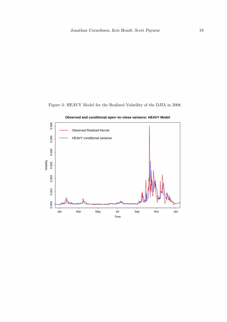
The list-item condvar is a (T ×K) xts-object containing the conditional variances. For thetraditional HEAVY model, Figure 3 plots for example the conditional close-to-close variancefor the DJIA for 1996 up to 2009 (see next subsection for more information).

Examples

Fitting the HEAVY model on the Dow Jones Industrial Average from 1996 up to 2009As a first step, we load the realized_library (Heber et al. 2009) which contains informationon the Dow Jones Industrial Average. We then select from this library the daily returns andthe daily Realized Kernel estimates (Barndorff-Nielsen et al. 2004). The data matrix thatserves as an input for the heavyModel now has the returns as the first column and theRealized Kernel estimates in the second column. We further set the argument backcast tothe variance of the daily returns and the average realized kernel over the sample period.Wenow have all ingredients to estimate the HEAVY Model. Based on the output of the model,Figure 3 plots the conditional open-to-close variance, as estimated by the second equation inthe model. Note the striking peak in 2008 at the start of the financial crisis.

> # Implementation of the heavy model on DJIA:

> data("realized_library");

> returns = realized_library$Dow.Jones.Industrials.Returns;

> rk = realized_library$Dow.Jones.Industrials.Realized.Kernel;

> returns = returns[!is.na(rk)]; rk = rk[!is.na(rk)]; # Remove NA's> data = cbind( returns^2, rk );

> backcast = matrix( c(var(returns),mean(rk)) ,ncol=1);

>

> startvalues = c(0.004,0.02,0.44,0.41,0.74,0.56); # Initial values

> output = heavyModel( data = as.matrix(data,ncol=2), compconst=FALSE,

+ startingvalues = startvalues, backcast=backcast);

> output$estparams

[,1]

omega1 0.01750506

omega2 0.06182249

alpha1 0.45118753

alpha2 0.41204541

beta1 0.73834594

beta2 0.56367558

6. Liquidity

6.1. Matching trades and quotes

Trades and quotes are often supplied as separate data objects. For many research and practicalquestions related to transaction data, one needs to merge trades and quotes. Since trades and


Figure 3: HEAVY Model for the Realized Volatility of the DJIA in 2008.

Jan Mar May Jul Sep Nov Jan

0.00

00.

001

0.00

20.

003

0.00

40.

005

0.00

6

Time

Vol

atili

ty

Observed and conditional open−to−close variance: HEAVY Model

Observed Realized Kernel

HEAVY conditional variance


Table 4: Overview of Liquidity measures

Argument(s) Liquidity measures

es, rs Compute effective (realized) spreadvalue trade Compute trade value (price × size)signed value trade Compute signed trade valuesigned trade size Compute signed trade sizedi diff, di div Compute depth imbalancepes, prs Compute proportional effective and realized spreadprice impact, prop price impact Compute price impacttspread, pts Compute half traded and proportional half-traded spreadqs, logqs Compute quoted spreadqsslope, logqslope Compute quoted slope

quotes can be subject to different reporting lags, this is not a straightforward operation (Leeand Ready 1991). The function matchTradesQuotes can be used for matching trades andquotes. One should supply the number of seconds quotes are registered faster than trades.Based on the research of Vergote (2005), we set 2 seconds as the default.

6.2. Inferred trade direction

Many trades and quotes databases do not indicate whether individual trades are market buyor market sell orders. highfrequency implements with getTradeDirection the Lee-Readyrule (Lee and Ready 1991) to infer the trade direction based on the matched trades andquotes.

6.3. Liquidity measures

Numerous liquidity measures can be calculated based on matched trade and quote data,using the function tqLiquidity (see Bessembinder (2003), Boehmer (2005), Hasbrouck andSeppi (2001) and Venkataraman (2001) for more information on the implemented liquiditymeasures). The main implemented liquidity measures are listen in Table 4, and can be usedas arguments of the function tqLiquidity.

The example below illustrates how to: (i) match trades and quotes, (ii) get the trade directionand (iii) calculate liquidity measures.

> #Load data samples


> data("sample_qdata");

> #Match the trade and quote data

> tqdata = matchTradesQuotes(sample_tdata,sample_qdata);

> #Display information in tqdata

> colnames(tqdata)[1:6];

[1] "SYMBOL" "EX" "PRICE" "SIZE" "COND" "CORR"


> colnames(tqdata)[7:12];

[1] "G127" "BID" "BIDSIZ" "OFR" "OFRSIZ" "MODE"

> #Get the inferred trade direction according to the Lee-Ready rule

> x = getTradeDirection(tqdata);

> #Calculate the proportional realized spread:

> prs = tqLiquidity(tqdata,sample_tdata,sample_qdata,type="prs");

> #Calculate the effective spread:

> es = tqLiquidity(tqdata,type="es");

7. Acknowledgements:

We thank Google for the financial support through the Google summer of code 2012 pro-gram. Furthermore, we thank the participants of the 1st R/Rmetrics Summer School and 4thUser/Developer Meeting on Computational Finance and Financial Engineering, Switzerland(2010) and the ”R/Finance: Applied finance with R” conference, USA, Chicago (2010), fortheir comments and suggestions. In particular, we thank Christophe Croux, Brian Petersonand Eric Zivot for their insights and help in developing this package. Financial support fromthe Flemish IWT (Institute for Science and Innovation), the National Bank of Belgium andthe Research Fund K.U.Leuven is gratefully acknowledged.

References

Ait-Sahalia Y, Mykland PA, Zhang L (2005). “A Tale of Two Time Scales: DeterminingIntegrated Volatility With Noisy High-Frequency Data.” Journal of the American StatisticalAssociation, 100, 1394–1411.

Andersen TG, Bollerslev T (1997). “Intraday periodicity and volatility persistence in financialmarkets.” Journal of Empirical Finance, 4, 115–158.

Andersen TG, Bollerslev T, Diebold F (2007). “Roughing it up: including jump components inthe measurement, modelling and forecasting of return volatility.” The Review of Economicsand Statistics, 89, 701–720.

Andersen TG, Bollerslev T, Diebold F, Labys P (2003). “Modeling and forecasting realizedvolatility.” Econometrica, 71, 579–625.

Andersen TG, Dobrev D, Schaumburg E (2012). “Jump-Robust Volatility Estimation usingNearest Neighbor Truncation.” Journal of Econometrics, 169, 75–93.

Barndorff-Nielsen OE, Hansen PR, Lunde A, Shephard N (2004). “Regular and modifiedkernel-based estimators of integrated variance: The case with independent noise.” Workingpaper.

Barndorff-Nielsen OE, Hansen PR, Lunde A, Shephard N (2008). “Realised Kernels in Prac-tice: Trades and Quotes.” Econometrics Journal, 4, 1–32.


Barndorff-Nielsen OE, Hansen PR, Lunde A, Shephard N (2011). “Multivariate realisedkernels: consistent positive semi-definite estimators of the covariation of equity prices withnoise and non-synchronous trading.” Journal of Econometrics, 162, 149–169.

Barndorff-Nielsen OE, Shephard N (2004). “Measuring the impact of jumps in multivari-ate price processes using bipower covariation.” Discussion paper, Nuffield College, OxfordUniversity.

Bessembinder H (2003). “Issues in Assessing Trade Execution Costs.” Journal of FinancialMarkets, 6, 223–257.

Boehmer E (2005). “Dimensions of execution quality: Recent evidence for US equity markets.”Journal of Financial Economics, 78, 553–582.

Boudt K, Croux C, Laurent S (2011a). “Outlyingness weighted covariation.” Journal ofFinancial Econometrics, 9, 657–684.

Boudt K, Croux C, Laurent S (2011b). “Robust estimation of intraweek periodicity in volatilityand jump detection.” Journal of Empirical Finance, 18, 353–367.

Boudt K, Zhang J (2010). “Jump robust two time scale covariance estimation and realizedvolatility budgets.” Mimeo.

Brownlees C, Gallo G (2006). “Financial econometric analysis at ultra-high frequency: Datahandling concerns.” Computational Statistics & Data Analysis, 51, 2232–2245.

Cornelissen J, Boudt K (2012). RTAQ: Tools for the analysis of trades and quotes in R. Rpackage version 0.2, URL http://CRAN.R-project.org/package=RTAQ.

Corsi F (2009a). “A Simple Approximate Long Memory Model of Realized Volatility.” Journalof Financial Econometrics, 7, 174–196.

Corsi F (2009b). “A Simple Long Memory Model of Realized Volatility.” Journal of FinancialEconometrics, 7, 174–196.

Corsi F, Reno R (2012). “Discrete-time volatility forecasting with persistent leverage effectand the link with continuous-time volatility modeling.” Journal of Business and EconomicStatistics, p. forthcoming.

De Pooter M, Martens MP, Van Dijk DJ (2008). “Predicting the Daily Covariance Matrixfor S&P 100 Stocks using Intraday Data - But Which Frequency to Use?” EconometricReviews, 27, 199–229.

Fleming J, Kirby C, Ostdiek B (2003). “The Economic Value of Volatility Timing Using”Realized” Volatility.” Journal of Financial Economics, 67, 473–509.

Gobbi F, Mancini C (2009). “Identifying the covariation between the diffusion parts and theco-jumps given discrete observations.” Mimeo.

Harris F TMGS, Wood R (1995). “Cointegration, error correction, and price discovery oninfomationally linked security markets.” Journal of Financial and Quantitative Analysis,30, 563–581.

http://CRAN.R-project.org/package=RTAQ


Hasbrouck J, Seppi DJ (2001). “Common Factors in Prices, Order Flows and Liquidity.”Journal of Financial Economics, 59, 383–411.

Hayashi T, Yoshida N (2005). “On covariance estimation of non-synchronously observeddiffusion processes.” Bernoulli, 11, 359–379.

Heber G, Lunde A, Shephard N, Sheppard K (2009). “Oxford-Man Institute’s realized library,version 0.1.” ”, Oxford-Man Institute, University of Oxford.

Lee CMC, Ready MJ (1991). “Inferring Trade Direction from Intraday Data.” Journal ofFinance, 46, 733–746.

Payseur S (2008). realized: Realized. R package version 0.81, URL http://cran.r-project.

org/web/packages/realized/realized.pdf.

Ryan JA (2011). quantmod: Quantitative Financial Modelling Framework. R package version0.3-17, URL http://CRAN.R-project.org/package=quantmod.

Ryan JA, Ulrich JM (2009). xts: Extensible Time Series. R package version 0.6-7, URLhttp://CRAN.R-project.org/package=xts.

Shephard N, Sheppard K (2010). “Realising the future: forecasting with high frequency basedvolatility (HEAVY) models.” Journal of Applied Econometrics, 25, 197–231.

Venkataraman K (2001). “Automated Versus Floor Trading: An Analysis of Execution Costson the Paris and New York Exchanges.” The Journal of Finance, 56, 1445–1485.

Vergote O (2005). “How to Match Trades and Quotes for NYSE Stocks?” K.U.Leuven workingpaper.

Yan B, Zivot E (2003). “Analysis of High-Frequency Financial Data with S-Plus.” UWEC-2005-03. URL http://ideas.repec.org/p/udb/wpaper/uwec-2005-03.html.

Zhang L (2011). “Estimating covariation: Epps effect, microstructure noise.” Journal ofEconometrics, 160, 33–47.

Affiliation:

Kris BoudtVU University Amsterdam, Lessius and K.U.Leuven, BelgiumE-mail: [email protected]

Jonathan CornelissenK.U.Leuven, BelgiumE-mail: [email protected]

Scott PayseurDirector at UBS Global Asset ManagementE-mail: [email protected]

http://cran.r-project.org/web/packages/realized/realized.pdf

http://cran.r-project.org/web/packages/realized/realized.pdf

http://CRAN.R-project.org/package=quantmod

http://CRAN.R-project.org/package=xts

http://ideas.repec.org/p/udb/wpaper/uwec-2005-03.html

mailto:[email protected]



highfrequency: toolkit for the analysis of highfrequency ... · pdf filehighfrequency: toolkit...

Documents