higher-dimensional knots according to michel kervaire
TRANSCRIPT
Series of Lectures in Mathematics
Michel/Weber | Rotis Sans | Pantone 287, Pantone 116 | 170 x 240 mm | RB: 7.2 mm
Françoise MichelClaude Weber
Higher-Dimensional Knots According to Michel Kervaire
Michel Kervaire wrote six papers on higher-dimensional knots which can be considered fundamental to the development of the theory. They are not only of historical interest but naturally introduce to some of the essential techniques in this fascinating area.
This book is written to provide graduate students with the basic concepts necessary to read texts in higher-dimensional knot theory and its relations with singularities. The first chapters are devoted to a presentation of Pontrjagin’s construction, surgery and the work of Kervaire and Milnor on homotopy spheres. We pursue with Kervaire’s fundamental work on the group of a knot, knot modules and knot cobordism. We add developments due to Levine. Tools (like open books, handlebodies, plumbings, …) often used but hard to find in original articles are presented in appendices. We conclude with a description of the Kervaire invariant and the consequences of the Hill–Hopkins–Ravenel results in knot theory.
ISBN 978-3-03719-180-4
www.ems-ph.org
Françoise Michel and Claude W
eberH
igher-Dimensional Knots According to M
ichel Kervaire
Françoise MichelClaude Weber
Higher-Dimensional Knots According to Michel Kervaire


EMS Series of Lectures in MathematicsEdited by Ari Laptev (Imperial College, London, UK)
EMS Series of Lectures in Mathematics is a book series aimed at students, professional mathematicians and scientists. It publishes polished notes arising from seminars or lecture series in all fields of pure and applied mathematics, including the reissue of classic texts of continuing interest. The individual volumes are intended to give a rapid and accessible introduction into their particular subject, guiding the audience to topics of current research and the more advanced and specialized literature.
Previously published in this series (for a complete listing see our homepage at www.ems-ph.org):Sergey V. Matveev, Lectures on Algebraic TopologyJoseph C. Várilly, An Introduction to Noncommutative GeometryReto Müller, Differential Harnack Inequalities and the Ricci FlowEustasio del Barrio, Paul Deheuvels and Sara van de Geer, Lectures on Empirical ProcessesIskander A. Taimanov, Lectures on Differential GeometryMartin J. Mohlenkamp and María Cristina Pereyra, Wavelets, Their Friends, and What They
Can Do for YouStanley E. Payne and Joseph A. Thas, Finite Generalized QuadranglesMasoud Khalkhali, Basic Noncommutative GeometryHelge Holden, Kenneth H. Karlsen, Knut-Andreas Lie and Nils Henrik Risebro, Splitting Methods
for Partial Differential Equations with Rough SolutionsKoichiro Harada, “Moonshine” of Finite GroupsYurii A. Neretin, Lectures on Gaussian Integral Operators and Classical GroupsDamien Calaque and Carlo A. Rossi, Lectures on Duflo Isomorphisms in Lie Algebra and
Complex GeometryClaudio Carmeli, Lauren Caston and Rita Fioresi, Mathematical Foundations of SupersymmetryHans Triebel, Faber Systems and Their Use in Sampling, Discrepancy, Numerical IntegrationKoen Thas, A Course on Elation QuadranglesBenoît Grébert and Thomas Kappeler, The Defocusing NLS Equation and Its Normal FormArmen Sergeev, Lectures on Universal Teichmüller SpaceMatthias Aschenbrenner, Stefan Friedl and Henry Wilton, 3-Manifold GroupsHans Triebel, Tempered Homogeneous Function SpacesKathrin Bringmann, Yann Bugeaud, Titus Hilberdink and Jürgen Sander, Four Faces of Number
TheoryAlberto Cavicchioli, Friedrich Hegenbarth and Dušan Repovš, Higher-Dimensional Generalized
Manifolds: Surgery and ConstructionsDavide Barilari, Ugo Boscain and Mario Sigalotti, Geometry, Analysis and Dynamics on sub-
Riemannian Manifolds, Volume IDavide Barilari, Ugo Boscain and Mario Sigalotti, Geometry, Analysis and Dynamics on sub-
Riemannian Manifolds, Volume IIDynamics Done with Your Bare Hands, Françoise Dal’Bo, François Ledrappier and Amie Wilkinson,
(Eds.)Hans Triebel, PDE Models for Chemotaxis and Hydrodynamics in Supercritical Function Spaces
Higher-DimensionalKnots Accordingto Michel Kervaire
Françoise MichelClaude Weber
Claude WeberSection de MathématiquesUniversité de Genève2-4 rue de Lièvre, C.P. 641211 Genève 4Switzerland
E-mail: [email protected]
Authors:
Françoise MichelInstitut de Mathématiques de ToulouseUniversité Paul Sabatier118 route de Narbonne31062 Toulouse Cedex 9France
E-mail: [email protected]
2010 Mathematics Subject Classification: 57Q45, 57R65, 32S55
Key words: Knots in high dimensions, homotopy spheres, complex singularities
ISBN 978-3-03719-180-4
The Swiss National Library lists this publication in The Swiss Book, the Swiss national bibliography, and the detailed bibliographic data are available on the Internet at http://www.helveticat.ch.
This work is subject to copyright. All rights are reserved, whether the whole or part of the material is concerned, specifically the rights of translation, reprinting, re-use of illustrations, recitation, broadcasting, reproduction on microfilms or in other ways, and storage in data banks. For any kind of use permission of the copyright owner must be obtained.
© 2017 European Mathematical Society
Contact address: European Mathematical Society Publishing House Seminar for Applied Mathematics ETH-Zentrum SEW A21 CH-8092 Zürich Switzerland
Email: [email protected] Homepage: www.ems-ph.org
Typeset using the authors’ TEX files: Alison Durham, Manchester, UKPrinting and binding: Beltz Bad Langensalza GmbH, Bad Langensalza, Germany∞ Printed on acid free paper9 8 7 6 5 4 3 2 1

Preface
The aim of this book is to present Kervaire’s work on differentiable knots in higherdimensions in codimension q = 2. As explained in our introduction (see Section 1.7),this book is written to make the reading of papers by Michel Kervaire and JeromeLevine easier. Thus we hope to communicate our enthusiasm for higher-dimensionalknot theory. In order to appreciate the importance of Kervaire’s contribution, wedescribe in Chapters 2 to 4 what was, at the time, the situation in differential topologyand in knot theory in codimension q ≥ 3. In Chapter 5, we expose Kervaire’scharacterization of the fundamental group of a knot complement. In Chapter 6,we explain Kervaire and Levine’s work on knot modules. In Chapter 7, we detailKervaire’s construction of the “simple knots” classified by Jerome Levine. Chapter 8summarizes Kervaire and Levine’s results on knot cobordism. In Chapter 9, weapply higher-dimensional knot theory to singularities of complex hypersurfaces.Appendixes A to D are devoted to a discussion of some basic concepts, known to theexperts: signs, Seifert hypersurfaces, open book decompositions and handlebodies.In Appendix E, we conclude with an exposition of the results of Hill–Hopkins–Ravenel on the Kervaire invariant problem and its consequences for knot theory incodimension 2.
The point of view adopted here is somewhat pseudo-historical. When we makeexplicit Kervaire’s work we try to follow him closely, in order to retain some of theflavor of the original texts. When necessary we add further contributions, often dueto Levine. We also propose developments that occurred later.
We thank Peter Landweber for patiently correcting our English. The figures inAppendix F are due to Cam Van Quach. We thank her for her friendly collaboration.
Françoise MichelClaude Weber
Geneva, September 2016


Contents
Preface . . . . . . . . . . . . . . . . . . . . . . . . . . . . . . . . . . . . . . v
1 Introduction . . . . . . . . . . . . . . . . . . . . . . . . . . . . . . . . . . 11.1 Kervaire’s six papers on knot theory . . . . . . . . . . . . . . . . . 11.2 A brief description of the content of the book . . . . . . . . . . . . 21.3 What is a knot? . . . . . . . . . . . . . . . . . . . . . . . . . . . . 31.4 Knots in the early 1960s . . . . . . . . . . . . . . . . . . . . . . . 41.5 Higher-dimensional knots and homotopy spheres . . . . . . . . . . 41.6 Links and singularities . . . . . . . . . . . . . . . . . . . . . . . . 51.7 Final remarks . . . . . . . . . . . . . . . . . . . . . . . . . . . . . 61.8 Conventions and notation . . . . . . . . . . . . . . . . . . . . . . . 7
2 Some tools of differential topology . . . . . . . . . . . . . . . . . . . . . . 92.1 Surgery from an elementary point of view . . . . . . . . . . . . . . 92.2 Vector bundles and parallelizability . . . . . . . . . . . . . . . . . 102.3 The Pontrjagin method and the J-homomorphism . . . . . . . . . . 11
3 The Kervaire–Milnor study of homotopy spheres . . . . . . . . . . . . . . 153.1 Homotopy spheres . . . . . . . . . . . . . . . . . . . . . . . . . . 153.2 The groups Θn and bPn+1 . . . . . . . . . . . . . . . . . . . . . . . 153.3 The Kervaire invariant . . . . . . . . . . . . . . . . . . . . . . . . 203.4 The groups Pn+1 . . . . . . . . . . . . . . . . . . . . . . . . . . . 223.5 The Kervaire manifold . . . . . . . . . . . . . . . . . . . . . . . . 24
4 Differentiable knots in codimension ≥3 . . . . . . . . . . . . . . . . . . . 274.1 On the isotopy of knots and links in any codimension . . . . . . . . 274.2 Embeddings and isotopies in the stable and metastable ranges . . . . 284.3 Below the metastable range . . . . . . . . . . . . . . . . . . . . . . 29
5 The fundamental group of a knot complement . . . . . . . . . . . . . . . . 335.1 Homotopy n-spheres embedded in Sn+2 . . . . . . . . . . . . . . . 335.2 Necessary conditions to be the fundamental group of a knot complement 355.3 Sufficiency of the conditions if n ≥ 3 . . . . . . . . . . . . . . . . . 375.4 The Kervaire conjecture . . . . . . . . . . . . . . . . . . . . . . . . 405.5 Groups that satisfy the Kervaire conditions . . . . . . . . . . . . . . 41

viii Contents
6 Knot modules . . . . . . . . . . . . . . . . . . . . . . . . . . . . . . . . . 436.1 The knot exterior . . . . . . . . . . . . . . . . . . . . . . . . . . . 436.2 Some algebraic properties of knot modules . . . . . . . . . . . . . . 456.3 The qth knot module when q < n/2 . . . . . . . . . . . . . . . . . 486.4 Seifert hypersurfaces . . . . . . . . . . . . . . . . . . . . . . . . . 506.5 Odd-dimensional knots and the Seifert form . . . . . . . . . . . . . 526.6 Even-dimensional knots and the torsion Seifert form . . . . . . . . . 56
7 Odd-dimensional simple links . . . . . . . . . . . . . . . . . . . . . . . . 617.1 q-handlebodies . . . . . . . . . . . . . . . . . . . . . . . . . . . . 617.2 The realization theorem for Seifert matrices . . . . . . . . . . . . . 627.3 Levine’s classification of embeddings of handlebodies in codimension 1 657.4 Levine’s classification of simple odd-dimensional knots . . . . . . . 67
8 Knot cobordism . . . . . . . . . . . . . . . . . . . . . . . . . . . . . . . . 698.1 Definitions . . . . . . . . . . . . . . . . . . . . . . . . . . . . . . . 698.2 The even-dimensional case . . . . . . . . . . . . . . . . . . . . . . 698.3 The odd-dimensional case . . . . . . . . . . . . . . . . . . . . . . 71
9 Singularities of complex hypersurfaces . . . . . . . . . . . . . . . . . . . 759.1 The theory of Milnor . . . . . . . . . . . . . . . . . . . . . . . . . 759.2 Algebraic links and Seifert forms . . . . . . . . . . . . . . . . . . . 789.3 Cobordism of algebraic links . . . . . . . . . . . . . . . . . . . . . 799.4 Examples of Seifert matrices associated to algebraic links . . . . . . 809.5 Mumford and topological triviality . . . . . . . . . . . . . . . . . . 819.6 Joins and Pham–Brieskorn singularities . . . . . . . . . . . . . . . 839.7 The paper by Kauffman [56] . . . . . . . . . . . . . . . . . . . . . 869.8 The paper by Kauffman and Neumann [57] . . . . . . . . . . . . . 879.9 Kauffman–Neumann’s construction when both links are the binding
of an open book decomposition . . . . . . . . . . . . . . . . . . . . 88
A Linking numbers and signs . . . . . . . . . . . . . . . . . . . . . . . . . . 91A.1 The boundary of an oriented manifold . . . . . . . . . . . . . . . . 91A.2 Linking numbers . . . . . . . . . . . . . . . . . . . . . . . . . . . 92
B Existence of Seifert hypersurfaces . . . . . . . . . . . . . . . . . . . . . . 93
C Open book decompositions . . . . . . . . . . . . . . . . . . . . . . . . . . 95C.1 Open books . . . . . . . . . . . . . . . . . . . . . . . . . . . . . . 95C.2 Browder’s lemma 2 . . . . . . . . . . . . . . . . . . . . . . . . . . 96
Contents ix
D Handlebodies and plumbings . . . . . . . . . . . . . . . . . . . . . . . . . 99D.1 Bouquets of spheres and handlebodies . . . . . . . . . . . . . . . . 99D.2 Parallelizable handlebodies . . . . . . . . . . . . . . . . . . . . . . 101D.3 m-dimensional spherical links in S2m+1 . . . . . . . . . . . . . . . 103D.4 Plumbing . . . . . . . . . . . . . . . . . . . . . . . . . . . . . . . 104
E Homotopy spheres embedded in codimension 2 and the Kervaire–Arf–-Robertello–Levine invariant . . . . . . . . . . . . . . . . . . . . . . . . . 109E.1 Which homotopy spheres can be embedded in codimension 2? . . . 109E.2 The Kervaire–Arf–Robertello–Levine invariant . . . . . . . . . . . 111E.3 The Hill–Hopkins–Ravenel result and its influence on the KARL
invariant . . . . . . . . . . . . . . . . . . . . . . . . . . . . . . . . 112
F Figures . . . . . . . . . . . . . . . . . . . . . . . . . . . . . . . . . . . . 115
Bibliography . . . . . . . . . . . . . . . . . . . . . . . . . . . . . . . . . . . 121
Index of Notation . . . . . . . . . . . . . . . . . . . . . . . . . . . . . . . . . 129
Index of Quoted Theorems . . . . . . . . . . . . . . . . . . . . . . . . . . . . 131
Index of Terminology . . . . . . . . . . . . . . . . . . . . . . . . . . . . . . . 133


1
Introduction
1.1 Kervaire’s six papers on knot theory
Michel Kervaire wrote six papers on knots: [63], [64], [66], [45], [46], and [69].The first one is both an account of Kervaire’s talk at a symposium held at Princeton
in spring 1963 in honor ofMarstonMorse and a report of discussions between severalparticipants in the symposium about Kervaire’s results. Reading this paper is reallyfascinating, since one sees higher-dimensional knot theory emerging. The subject isthe fundamental group of knots in higher dimensions.
The second one is the written thesis that Kervaire presented in Paris in June 1964.In fact Kervaire had already obtained a PhD in Zurich under Heinz Hopf in 1955,but in 1964 he applied for a position in France and, at that time, a French thesis wascompulsory. In the end, the appointment did not materialize. But the thesis textremains as an article published in the Bulletin de la S.M.F. ([64]). As this articleis the main reason for writing this text, we name it Kervaire’s Paris paper. It isthe most important one that Kervaire wrote on knot theory. It can be considered tobe the foundational text on knots in higher dimensions, together with contemporarypapers by Jerome Levine ([77], [78], and [79]). One should also add to the list theHirsch–Neuwirth paper [50], which seems to be a development of discussions heldduring the Morse symposium.
To briefly present the subject of Kervaire’s Paris paper, we need a few definitions.A knot Kn ⊂ Sn+2 is the image of a differentiable embedding of an n-dimensionalhomotopy sphere in Sn+2. Its exterior E(K) is the complement of an open tubularneighborhood. The exterior has the homology of the circle S1 by Alexander duality.In short, the subject is the determination of the first homotopy group πq(E(K)), whichis different from πq(S1).
Later, Kervaire complained that he had to rush to complete this Paris paper indue time and he had doubts about the quality of its redaction. In fact we find thisarticle to be well written. The exposition is concise and clear, typically in Kervaire’sstyle. The pace is slow in parts that present a difficulty and fast when things areobvious. Now, what was obvious to Kervaire in spring 1964? Among other things,clearly Pontrjagin’s construction and surgery. As these techniques are possibly notso well known to a reader fifty years later, we devote Chapters 2 and 3 of this text toa presentation of these matters.
The last chapter of Kervaire’s Paris paper is a first attempt at understanding thecobordism of knots in higher dimensions. It contains a complete proof that an even-
2 1 Introduction
dimensional knot is always cobordant to a trivial knot. For odd-dimensional knots,the subject has a strong algebraic flavor, much related to the isometry groups ofquadratic forms and to algebraic number theory. Kervaire liked this algebraic aspectand devoted his third paper [66] to it.
Levine spent the first months of 1977 in Geneva and he gave wonderful lectureson many aspects of knot theory. His presence had a deep influence on severalmembers of the audience, including the two authors of this text! Under his initiativea meeting was organized by Kervaire in Les Plans-sur-Bex in March 1977. Theproceedings are recorded in the Springer Lecture Notes volume 685, edited by Jean-Claude Hausmann. The irony of history is that it was precisely at this time thatWilliam Thurston made his first announcements, which soon completely shatteredclassical knot theory and 3-manifolds. See Cameron Gordon’s paper [38, p. 44] inthe proceedings. The meeting renewed Kervaire’s interest in knot theory, and in thefollowing months he wrote his last three papers on the subject.
1.2 A brief description of the content of the book
As promised, we devote Chapters 2 and 3 to some background in differential topol-ogy, mainly vector bundles, Pontrjagin’s construction, and surgery, culminating withKervaire–Milnor.
We felt it necessary to devote Chapter 4 to knots in codimension ≥3. Its readingis optional. One reason to do so is that the subject was flourishing at the time,thanks to the efforts of André Haefliger and Levine. It is remarkable that Levine waspresent in both fields. Another reason is that the two subjects are in sharp contrast.Very roughly speaking one could say that it is a matter of fundamental group. Incodimension ≥3 the fundamental group of the exterior is always trivial while it isnever so in codimension 2. But more must be said. In codimension ≥3 there areno PL knots, as proved by Christopher Zeeman [137]. Hence everything is a matterof comparison between PL and DIFF. This is the essence of Haefliger’s theory ofsmoothing, written a bit later. On the contrary, in codimension 2 the theories of PLknots and of DIFF knots do not differ much.
In Chapter 5 we present Kervaire’s determination of the fundamental group ofknots in higher dimensions, together with some of the results from his two paperswritten with Jean-Claude Hausmann about the commutator subgroup and the centerof these groups. Some later developments are also presented.
Chapter 6 exposes Kervaire’s results on the first homotopy group πq(E(K)), whichis different from πq(S1). For q ≥ 2 these groups are in factZ[t, t−1]-modules. Indeed,Kervaire undertakes a first study of such modules, later to be called knot modules byLevine. In our presentation, we include several developments due to Levine.

1.3 What is a knot? 3
Up to Kervaire’s Paris paper, most of the effort in knot theory went into theconstruction of knot invariants. They produce necessary conditions for two knotsto be equivalent. In Levine’s paper [78] a change took place. From Dale Trotter’swork it was known that for classical knots, Seifert matrices of equivalent knots areS-equivalent. Levine introduced a class of odd-dimensional knots (he called themsimple knots) for which the S-equivalence of the Seifert matrices is both necessaryand sufficient for two knots to be isotopic. This is a significant classification result.Indeed, simple knots are already present in Kervaire’s Paris paper, but he did notpursue their study that far. Technically, the success of Levine’s study is largelydue to the fact that these knots bound a very special kind of Seifert hypersurface:a (parallelizable) handlebody. In Chapter 7 we present Levine’s work on odd-dimensional simple knots.
Chapter 8 is devoted to higher-dimensional knot cobordism. Levine reduced thedetermination of these groups to an algebraic problem. A key step in the argumentrests on the fact that each knot is cobordant to a simple knot.
In knot theory, the handlebodies one deals with are parallelizable and their bound-ary is a homotopy sphere. If we keep the parallelizability condition but admit anyboundary, the Kervaire–Levine arguments are still valid. This immediately applies tothe Milnor fiber of isolated singularities of complex hypersurfaces, as first noticed byMilnor himself and developed by Alan Durfee. Chapter 9 is devoted to that matter.It can be considered a prolongation of Kervaire and Levine’s work.
Appendixes A to E are of the kind that can be read independently. They providebasics, comments, and variations on subjects treated elsewhere in our book. InAppendix A we give our conventions on signs, which agree with those in Kauffman–Neumann [57]. This allows us to justify the signs for invariants of some basicalgebraic links (examples are given at the end of Chapter 9). Often, authors do notmention their sign conventions and hence one can find other signs in the literature. InAppendix Bwe prove the existence of Seifert hypersurfaces in amore general context.In Appendixes C and D, we present basics about open book decompositions andparallelizable handlebodies, which are useful in knot theory. Our aim in Appendix Eis to present the beautiful result by Mike Hill, Mike Hopkins, and Doug Ravenelabout the Kervaire invariant and to explain how this affects the theory of knots inhigher dimensions. It is a spectacular way to conclude this book.
A few figures, related to several sections of the book, are available in Appendix F.
1.3 What is a knot?
We use the following definitions.Definition 1.1. An n-link in Sn+q is a compact oriented differential submanifoldwithout boundary Ln ⊂ Sn+q . The integer q ≥ 1 is the codimension of the link. The

4 1 Introduction
n-links Ln1 and Ln
2 are equivalent if there exists a diffeomorphism f : Sn+q → Sn+q
such that f (Ln1 ) = Ln
2 , respecting the orientation of Sn+q and of the links.When Ln is a homotopy sphere, we say that Ln⊂Sn+q is an n-knot in codimen-
sion q.When Ln is the standard sphere Sn embedded in Sn+2, we say that Ln ⊂ Sn+2 is
a standard n-knot.The group of an n-link (resp. n-knot), Ln ⊂ Sn+2, is the fundamental group of
Sn+2 \ Ln.At the beginning of Chapter 4, we present the well-known proof that if two links
are equivalent there always exists a diffeomorphism f : Sn+q → Sn+q that is isotopicto the identity and moves one link to the other. Hence n-links are equivalent if andonly if they are isotopic.
In general the boundary of a Milnor fiber is not a homotopy sphere. It is amotivation to explain, in Chapter 7, how Kervaire and Levine’s works on simpleodd-dimensional knots can be generalized to simple links.
A link Ln ⊂ Sn+2 in codimension 2 is always the boundary of a (n+1)-dimensionaloriented smooth submanifold Fn+1 in Sn+2. We say that Fn+1 is a Seifert hypersur-face for Ln ⊂ Sn+2 ( some authors name it Seifert surface even when n ≥ 2).
1.4 Knots in the early 1960s
In the early 1960s, knots and links in S3 (which we call classical knots and links)had been deeply studied. Two objects played a central role in classical knot theory:the group of the knot and the Seifert surfaces. Despite the fact that, at that time,higher-dimensional topology was flourishing, knowledge about higher-dimensionalknots and links was very poor. The only interesting examples were obtained by thespinning construction, which goes back to Emil Artin, and by its generalization byChristopher Zeeman, called twist spinning. For example, if G is the group of aclassical knot, the spinning produces, for all n ≥ 2, an n-dimensional knot in Sn+2
having G as knot group. At that time, specialists knew that an n-link is alwaysthe boundary of an oriented, smooth, (n + 1)-dimensional submanifold of Sn+2.Here we call it a Seifert hypersurface of the link. A Seifert hypersurface is alwaysparallelizable.
1.5 Higher-dimensional knots and homotopy spheres
We recall, in Chapter 3, the results of Kervaire and Milnor [67] concerning the groupbPn+1 of n-dimensional homotopy spheres, which bound parallelizable manifolds.

1.6 Links and singularities 5
In particular, bPn+1 is trivial when (n + 1) is odd, and is a finite cyclic groupwhen (n + 1) is even. We also recall, in Appendix E (Proposition E.3), that anyelement of bPn+1 can be embedded in Sn+2. Conversely an n-dimensional homotopysphere embedded in Sn+1 is an element of bPn+1 because it is always the boundaryof a Seifert hypersurface that is parallelizable. These results lead us to definehigher-dimensional knots as embeddings of n-dimensional homotopy spheres in Sn+1.Kervaire had another reason to define higher-dimensional knots as embeddings ofhomotopy spheres. It is easier to construct higher-dimensional knots without havingto specify their differentiable structure. When n is even, an n-dimensional knot isalways a standard knot because bPn+1 is trivial. If n = 4k − 1, the signature of theintersection form of a Seifert hypersurface determines the differentiable structure ofits boundary. The case n = 4k + 1 is treated in Appendix E.
1.6 Links and singularities
The paper [97] by David Mumford marks the beginning of a new era since it puts alight on the role of the topology in studying complex singularities. In Section 9.5 weexplain some consequences of the following Mumford result:
Theorem 1.2. Let Σ be a normal complex surface. If the boundary L of point P ∈ Σis simply connected, then P is a regular point of Σ.
Mumford also introduces the concept of “plumbing” to describe the topology of agood resolution of a normal singular point of a complex surface. The reader has to becautious and should not confuse the plumbings obtained as good resolutions of normalgerms of complex hypersurfaces and what we call 2-handlebodies. As explained inAppendix D, following William Browder, there is a way to define 2q-plumbings asequivalent to q-handlebodies if q ≥ 4.
The connection between higher-dimensional homotopy spheres and isolated sin-gularities of complex hypersurfaces was established in spring 1966. The story isbeautifully (and movingly) told by Egbert Brieskorn in [16, pp. 30–52]. Severalmathematicians took part in the events: Egbert Brieskorn, Klaus Jänich, FriedrichHirzebruch, JohnMilnor, and John Nash. In June 1966 [15], Egbert Brieskorn provedthe following theorem, which is a corollary of his thorough study of the now-namedPham–Brieskorn singularities. The proof rests on the work of Frédéric Pham.
Theorem 1.3. Let Σ2q−1 be a (2q− 1)-homotopy sphere that bounds a parallelizablemanifold. Then there exist (q + 1) integers ai ≥ 2, 0 ≤ i ≤ q, such that the linkL f ⊂ S2q+1 associated to f (z0, . . . , zq) = Σ
i=qi=0 zai
i is a knot diffeomorphic to Σ2q−1.
With his book Singular Points of ComplexHypersurfaces [93], Milnor definitivelyrelates the theory of odd-dimensional links to the study of the embedded topology
6 1 Introduction
of a germ f : (Cq+1, 0) → (C, 0) with an isolated critical point at the origin in Cq+1.In Chapter 9, we recall many important results contained in [93]. In particular weexplain how Milnor associates a simple fibered link L2q−1
f∈ S2q+1
ε to f . Such a linkis called an algebraic link.
In [81], Levine gives, when q ≥ 2, a classification theorem for simple (2q − 1)-dimensional knots via the Seifert forms. The knot theory of Kervaire–Levine willdirectly meet the Milnor theory of algebraic links in a paper by Durfee [29]. Indeed,when q ≥ 3, Durfee shows that the classification theorem of Levine also gives a clas-sification theorem for algebraic links (always in terms of Seifert forms). Such resultsare based on the classification of q-handlebodies, which are defined in Appendix D.The classification of algebraic links associated to germs of surfaces inC3 is still open.
In Section 9.6, we present the notion of joins, followingMilnor’s paper [88]. Joinsappeared to describe the topology of a germ f = g ⊕ h : (Cn+m, 0) → (C, 0) whereg : (Cn, 0) → (C, 0) and h : (Cm, 0) → (C, 0) are germs of holomorphic functionswith an isolated critical point at the origin and
f (x1, . . . , xn, y1, . . . , ym) = g(x1, . . . , xn) + h(y1, . . . , ym).
It gives an inductivemethod to describe the topology of the Pham–Brieskorn singular-ities. Kauffman, [56], and Kauffman and Neumann, [57], inspired by the topologicalbehavior of links associated to germs of the type f = g⊕ h, constructed topologicallybig families of higher-dimensional links by induction on the dimension. They haveconstructions where they control the Seifert form, and others with fibered links wherethey control the open book decompositions.
1.7 Final remarks
The aim of this book is to pay tribute to Kervaire and to make his work on knotsof higher dimensions easier to read for younger generations of mathematicians.Basically it is a mathematical exposition text. Our purpose is not to write a historyof knots in higher dimensions. We apologize for not making a list of all papers inthe subject. When we present Kervaire’s work we try to follow him closely, in orderto retain some of the flavor of the original texts. When necessary, we add furthercontributions often due to Levine. We also propose developments that occurred later.With the passing of time, we find it important to present in detail results on thefundamental group of the knot complement and on simple odd-dimensional knots(and links). Indeed,
(1) the determination of the fundamental group of the knot complement played a keyrole at the beginning of higher-dimensional knot theory;

1.8 Conventions and notation 7
(2) higher odd-dimensional simple knots can be classified via their relations withhandlebodies; on the one hand this classification induces a classification up tocobordism, and on the other hand, it can be easily generalized to links associatedto isolated singular points of complex hypersurfaces.
We have wondered whether to include Levine’s name in the title of this text. Wehave decided not to, although he certainly is the cofounder of higher-dimensional knottheory. But Levine pursued his work much beyond these first years, while Kervairestopped publishing in the subject (too) early. Hence it would have been difficult tofind an equilibrium between them. In fact a study of Levine’s work in knot theoryshould be much longer than this text.
1.8 Conventions and notation
Manifolds and embeddings are C∞. Usually, manifolds are compact and oriented. Amanifold is closed if compact without boundary. The boundary of M is written bM ,its interior is M , and its closure is M . Let L be a closed oriented submanifold of aclosed oriented manifold M . We denote by N(L) a closed tubular neighborhood ofL in M and by E(L) the closure of M \ N(L), i.e., E(L) = M \ N(L). By definitionE(L) is the exterior of L in M .
Fibers of vector bundles are vector spaces over the field of real numbers R. Therank of a vector bundle over a connected base is the dimension of its fibers.


2
Some tools of differential topology
An extremely useful reference for this chapter and the next one is provided by AntoniKosinski’s book [72]. Basics about differentiable manifolds are beautifully presentedby Morris Hirsch in [49].
2.1 Surgery from an elementary point of view
Originally, surgery was “just” a way to transform a differentiable manifold intoanother one as in [91].
Definition 2.1. The (standard) sphere Sn of dimension n is the set of points x =(x0, x1, . . . , xn) ∈ Rn+1 such that
∑x2i = 1. The ball Bn+1 of dimension (n+ 1) is the
set of points x = (x0, x1, . . . , xn) ∈ Rn+1 such that∑
x2i ≤ 1. The open ball Bn+1 of
dimension (n + 1) is defined by∑
x2i < 1.
Consider the product of spheres Sa × Sb, a ≥ 0, b ≥ 0. This manifold is theboundary of Sa×Bb+1 and of Ba+1×Sb. Suppose now that we have (Sa×Bb+1) ⊂ M ′
where M ′ is a manifold of dimension m = a+b+1. If M ′ has a boundary, we supposethat the embedding is far from bM ′. We consider then M = M ′ \ (Sa × Bb+1) andwe construct M ′′ = M ∪ (Ba+1 × Sb) with M ∩ (Ba+1 × Sb) = Sa × Sb.
Definition 2.2. One says that M ′′ is obtained from M ′ by a surgery along Sa × 0.The manifold M is the common part of M ′ and M ′′.
Remarks. (1) The process is reversible: M ′ is obtained from M ′′ by surgery along0 × Sb.
(2) Note that M ′ is obtained from the common part M by attaching the cell eb+1 =u ×Bb+1 of dimension b+1 (for some u ∈ Sa) and then a cell em of dimensionm.
(3) Analogously, M ′′ is obtained from M by attaching the cell ea+1 = Ba+1 × v ofdimension a + 1 (for some v ∈ Sb) and then a cell of dimension m.
Definition 2.3. We call Sa×0 ⊂ M ′ and 0×Sb ⊂ M ′′ the scars of the surgeries.
For an example of surgery, see Figures F.4 and F.5.

10 2 Some tools of differential topology
2.2 Vector bundles and parallelizability
In order to apply surgery successfully, we need to know when a sphere that isdifferentiably embedded in a differentiable manifold has a trivial normal bundle.Here are some answers.
Definition 2.4. A vector bundle over a complex Xk is trivial if it is isomorphic to aproduct bundle. A trivialization is such an isomorphism.
Definition 2.5. A manifold is parallelizable if its tangent bundle τM is trivial.
Comment. Parallelizable manifolds were introduced and studied by Ernst Stiefel inhis thesis [121], written under the direction of Heinz Hopf. Both were looking forconditions satisfied by a manifold when it is the underlying space of a Lie group. Atrivialization was called a parallelism by Stiefel. He proved that, among spheres, S1,S3, S7 are parallelizable. The following result was proved by Kervaire [60] and alsoby Bott–Milnor [14]. A key step is provided by the Bott periodicity theorem [13].
Theorem 2.6. S1, S3, S7 are the only spheres that are parallelizable.
Notation. Let εr denote the trivial bundle of rank r over an unspecified basis.
Definition 2.7. A vector bundle η is stably trivial if η ⊕ εr is trivial for some integerr ≥ 0.
Proposition 2.8. Let Xk be a complex of dimension k. Let η be a vector bundle overXk of rank s with k < s. Suppose that η is stably trivial. Then it is trivial.
Proof. See [91, Lemma 4].
To be parallelizable is a very strong condition on a manifold, quite difficult tohandle. The next condition is easier to work with.
Definition 2.9. A manifold M is stably parallelizable if its tangent bundle is stablytrivial.
Comments. (1) If M is stably parallelizable then τM⊕ε1 is trivial, by the propositionabove.
(2) The same proposition implies that a compact connected manifold Mn withnonempty boundary is stably parallelizable if and only if it is parallelizable,since it has the homotopy type of a complex of dimension n − 1 and since theclassification of bundles depends only on the homotopy type of the base space.
(3) The standard embedding of Sn in Rn+1 shows that Sn is stably parallelizable forall n.

2.3 The Pontrjagin method and the J-homomorphism 11
(4) More generally, suppose that Mn is embedded in a stably parallelizable manifoldwith trivial normal bundle. Then Mn is stably parallelizable.
Proposition 2.10. Let Mn be a stably parallelizable manifold of dimension n, em-bedded in a stably parallelizable manifold WN of dimension N with N ≥ 2n + 1.Then the normal bundle ν of M in W is trivial.
Proof. SinceW is stably parallelizable, we have τW⊕ε1 = εN+1. Hence τM⊕ν⊕ε1 =εN+1. Since M is stably parallelizable we have ν ⊕ εn+1 = εN+1. Since the rank of νis strictly larger than the dimension of M , Proposition 2.8 applies.
Comments. (1) In practice, the last proposition is applied to perform surgery onembedded spheres in stably parallelizable manifolds.
(2) The proposition is not true in general if N = 2n. See the sections below aboutthe Kervaire invariant and about the groups Pn+1.
2.3 The Pontrjagin method and the J-homomorphism
The Pontrjagin method is also called the Thom–Pontrjagin method or construction.See [104] and [124]. Its importance lies in the fact that it ties together (stably) paral-lelizable manifolds and (stable) homotopy groups of spheres. Originally, Pontrjaginwished to compute homotopy groups of spheres via differential topology. In thehands of Kervaire and Milnor it provided the crucial link between homotopy groupsof spheres and groups of homotopy spheres. (The novice reader should breathedeeply and read the last sentence a second time.)
We can see in retrospect that Kervaire’s early work as a graduate student wasideal preparation for a young topologist in the 1950s. Heinz Hopf asked Kervaire toread Pontrjagin’s announcement note [103] and to provide proofs where needed. See[59, bottom p. 220]. Kervaire’s description of the starting point of his thesis is quitepremonitory: “Une variété fermée Mk étant plongée dans un espace euclidien Rn+k
avec un champ de repères normaux. . . ” (A closed manifold Mk being embedded ina Euclidean space Rn+k with a field of normal frames. . . .) See [59, middle p. 219].The first chapter of Kervaire’s thesis in Zurich is devoted to a detailed presentationof Pontrjagin’s construction.
Here is a short reminder about the Pontrjagin method. We shall need the stableversion of it only.
Let Mn be a closed stably parallelizable manifold. We do not assume that Mn isconnected. Choose an integer m such that m ≥ n + 2. By Whitney’s theorems [134]we can embed Mn in Sn+m and any two embeddings are isotopic. By Section 2.2 itsnormal bundle is trivial. We choose a trivialization τ of it. More precisely, we choose
12 2 Some tools of differential topology
m sections of the normal bundle e1, e2, . . . , em such that e1(x), e2(x), . . . , em(x) arelinearly independent for each x ∈ Mn. These sections provide a map ψ : (U; bU) →(Bm; bBm) where U denotes a closed tubular neighborhood of Mn in Sn+m. Thesphere Sm is identified with Bm/bBm. Let ψ : U/bU → Bm/bBm = Sm be theinduced map. Extend ψ to a map Ψ : Sm+n → Sm by sending the complement of Uin Sn+m to the smashed boundary bBm. It is easily verified that the homotopy classof Ψ depends only on (M, F). This is the essence of the Pontrjagin construction.
For short we call the couple (Mn ⊂ Sn+m, τ) a framed n-manifold (in facta manifold in Sn+m with a trivialization (framing) of its normal bundle). Twoframed n-manifolds Mn
i for i = 0, 1 are framed cobordant if there exists a framedWn+1 ⊂ Sn+m × I such that W ∩ Sn+m × i = Mi consistently with the framings.Framed cobordism classes constitute an abelian group Ωfr
n,m under disjoint union.Let us observe that homotopic trivializations give rise to framed cobordant manifoldsand hence produce the same element in Ωfr
n,m.
Theorem 2.11 (Pontrjagin isomorphism theorem). The Pontrjagin construction pro-vides an isomorphism between Ωfr
n,m and πn+m(Sm).
Proof. From the definition of the homotopy relation, we deduce that framed cobor-dant submanifolds in Sn+m give rise to homotopic maps Sn+m −→ Sm. Hence we geta homomorphism Ωfr
n,m −→ πn+m(Sm).To prove surjectivity, we argue as follows. Let f : Sn+m −→ Sm be a represen-
tative of some element in πn+m(Sm). Let P ∈ Sm be a regular value of f equippedwith a normal framing in Sm. Then, by transversality, f −1(P) = M is a framedsubmanifold of Sn+m and the Pontrjagin construction applied to M (essentially thesmashings) produces a map Sn+m −→ Sm that is homotopic to f .
Here now is the proof of injectivity. First remember that a map f : Sn+m −→ Sm
is homotopic to a constant if and only if it extends to a map f ∗ : Bn+m+1 −→ Sm.Suppose then that f is obtained by the Pontrjagin construction and that it representsthe trivial element of πn+m(Sm). Make f ∗ transversal to P ∈ Sm keeping it fixedon Sn+m. Again by transversality the framed submanifold in Sn+m that represents fbounds in Bn+m+1 the framed submanifold ( f ∗)−1(P). By the definition of framedcobordism it represents the trivial element of Ωfr
n,m.
The proof is clearly valid without stability assumptions. But since we assume thatm ≥ n+ 2, the groups πn+m(Sm) andΩfr
n,m are independent of m. We denote them byπSn and Ωfr
n . The group πSn is the nth stable homotopy group of spheres (also calledthe stable nth stem). By Jean-Pierre Serre’s thesis [112], πSn is a finite abelian group.
In [61] Kervaire gave interpretations of several constructions in the theory ofhomotopy groups of spheres via the Pontrjagin method. For instance, the methodyields an easy description of a family of homomorphisms originally due to Hopf andWhitehead. Let n ≥ 1 be a fixed integer and let m ≥ 1 be some variable integer.
2.3 The Pontrjagin method and the J-homomorphism 13
Consider the nth sphere Sn standardly embedded in Sn+m. Its normal bundle has astandard trivialization and hence (homotopy classes of) different trivializations are innatural bijection with πn(SOm). The Pontrjagin construction yields a homomorphismJn,m : πn(SOm) → πn+m(Sm). Ifm is largewith respect to n (precisely ifm ≥ (n+2)),the group πn(SOm) does not depend on m and is denoted by πn(SO). Moreover, thehomomorphism Jn,m does not depend on m.
Thus we get a homomorphism Jn : πn(SO) → πSn . This is the stable J-homomorphism in dimension n.
Just at the right time, Raoul Bott [13] computed the groups πn(SO). His celebratedresults, Bott periodicity, are as follows:
Theorem 2.12. Let n ≥ 1 be an integer: then,
(1) πn(SO) depends only on the residue class of n mod 8;
(2) πn(SO) is isomorphic to Z/2 if n ≡ 0 or 1 mod 8;
(3) πn(SO) is isomorphic to Z if n ≡ 3 or 7 mod 8;
(4) πn(SO) is equal to 0 in the four other cases n ≡ 2, 4, 5, 6 mod 8.
Frank Adams’ important results [4] about the stable J-homomorphism are statedin the next two theorems. The first one is indispensable for proving that a homotopysphere of dimension n is stably parallelizable when (n − 1) is congruent to 0 or1 mod 8. See Section 3.2.
Theorem 2.13. The homomorphism Jn is injective when πn(SO) is isomorphic toZ/2.
When πn(SO) is isomorphic to Z the image Im Jn ⊂ πSn is a finite cyclic subgroupwhose elements are by their very construction easy to describe. Hence it wasimportant to determine what this subgroup is. Milnor–Kervaire in [94] (with the helpof Atiyah–Hirzebruch [7] to get rid of a possible factor 2) gave a “lower bound” (i.e.,a factor) of its order. Then Adams proved that this “expected value” is the right one.Another possible factor 2 was eliminated by the proof of the Adams conjecture. See[5, pp. 529–532]. The proof of the Adams conjecture also established that Im Jn is adirect factor of πSn . The final statement follows:
Theorem 2.14. Let us write n = 4k − 1. Then the order of the image of J4k−1 :π4k−1(SO) → πS4k−1 is equal to the denominator den(Bk/4k) where Bk is the kthBernoulli number, indexed as by Friedrich Hirzebruch in [52].
We recall that this numbering is such that Bk > 0 for every k > 0 and that thesequence begins B1 = 1/6, B2 = 1/30, . . . . It is fortunate for topologists that thisdenominator is computable (it is the “easy part” of Bernoulli numbers, much relatedto von Staudt theorems). See [3] for explicit formulas.
14 2 Some tools of differential topology
Remark on the history. We have presented one of the early appearances of theJ-homomorphism. Many others followed. Here is one of them, also due to Kervaireand Milnor, but never published. Let ν be a very large integer. Let Gν be the set ofhomotopy equivalences of the sphere Sν−1. Let Oν be the orthogonal group of Rν .We have a natural inclusion Oν → Gν . Let us take the limit for ν going to infinity.We obtain a map J : O → G that induces a homomorphism πn(O) → πn(G). Thishomomorphism is equivalent, via an isomorphism between πSn and πn(G), to thehomomorphism Jn : πn(SO) → πSn defined above via the Pontrjagin construction. Itis the reason why the map J : O → G is also called the J-homomorphism.

3
The Kervaire–Milnor study of homotopy spheres
In this chapter we offer a summary of Kervaire–Milnor’s paper. The reader interestedonly in knot theory can safely skip over this chapter.
3.1 Homotopy spheres
Definition 3.1. A differential closed oriented manifold Σn of dimension n is a ho-motopy sphere if it has the homotopy type of the standard sphere Sn.Comments. (1) Classical results of algebraic topology imply that Σn is a homotopy
sphere if and only if π1(Σn) = π1(Sn) and Hi(Σ
n; Z) = Hi(Sn; Z) for all i =0, 1, . . . , n.
(2) When [67] was written it was just known (thanks to Stephen Smale and JohnStallings) that a homotopy sphere of dimension n ≥ 5 is in fact homeomorphicto the standard sphere Sn. See [116] and [118].
(3) It is known today that a homotopy sphere of dimension n is homeomorphic to Sn
for any value of n. In fact a stronger result is known. Consider a compact andconnected topological n-manifold that has the homotopy type of the n-sphere.Then this manifold is homeomorphic to Sn. We could say that “the topologicalPoincaré conjecture is true in all dimensions”. Stated in this form, the result isdue to Newman [101] for n ≥ 5 and to Freedman [36] for n = 4. The proof isclassical for n ≤ 2, but it uses the triangulation of surfaces. For n = 3 the proofis tortuous. First apply Moise [96] to triangulate the homotopy sphere. Thensmooth it by Munkres [98]. Finally apply Perelman!
Proposition 3.2. A homotopy sphere of dimension n ≥ 5 is diffeomorphic to thestandard sphere if and only if it bounds a contractible manifold.Proof. This is an immediate consequence of the Smale h-cobordism theorem.
3.2 The groups Θn and bPn+1
We consider the set Λn of oriented homotopy n-spheres up to orientation-preservingdiffeomorphism. On Λn a composition law is defined, called the connected sum

16 3 The Kervaire–Milnor study of homotopy spheres
and written Σ1]Σ2. See [90] for a comprehensive study of this operation. It iscommutative, associative, and has the standard sphere as the zero element. In otherwords, it is a commutative monoid. By the validity of the topological Poincaréconjecture, Λn classifies the oriented differential structures on the n-sphere up toorientation-preserving diffeomorphism. To avoid confusing readers who go throughpapers of the 1950s and 1960s, we keep the terminology “homotopy spheres”.
Definition 3.3. Let Wn+1 be an oriented compact (n + 1)-manifold and let Mn1 and
Mn2 be two oriented n-manifolds. Then Wn+1 is an oriented h-cobordism between
Mn1 and Mn
2 if
(1) the oriented boundary bW is diffeomorphic to Mn1∐−Mn
2 , where the − signdenotes the opposite orientation;
(2) both inclusions Mni → Wn+1 are homotopy equivalences.
Kervaire and Milnor prove that the h-cobordism relation is compatible with theconnected sum operation. The quotient of Λn by the h-cobordism equivalencerelation is an abelian group written Θn. The inverse of Σ is −Σ.Comments. (1) If n ≥ 5 by Smale’s h-cobordism theorem Θn is in fact isomorphic
to Λn. Note that Kervaire–Milnor say explicitly that their paper does not dependon Smale’s results. But of course Smale’s results are needed to interpret Θn interms of differential structures on Sn.
(2) Since homotopy spheres are oriented, a chirality question is present here. Ahomotopy sphere Σn is achiral (i.e., possesses an orientation-reversing diffeo-morphism) if and only if it represents an element of order ≤2 in Θn (assumen , 4).The starting point of [67] is the following result.
Theorem 3.4. Any homotopy sphere Σn is stably parallelizable.
Rough idea of the proof. We first need a definition.
Definition 3.5. A closed connected differentiable manifold Mn is almost paralleliz-able if Mn \ x or equivalently Mn \ Bn is parallelizable.
Clearly a homotopy sphere is almost parallelizable. For an almost parallelizablemanifold Mn there is one obstruction to stable parallelizability, which is an elementof πn−1(SO). By Pontrjagin construction this obstruction lies in the kernel of theJ-homomorphism. If πn−1(SO) is isomorphic to Z/2 by Adams’ theorem the J-homomorphism is injective in these dimensions and hence the obstruction vanishes.If πn−1(SO) is isomorphic to Z, a nonzero multiple of the obstruction is equal to thesignature of Mn and hence equal to 0 if Mn is a homotopy sphere.

3.2 The groups Θn and bPn+1 17
Comment. In fact the argument proves the following result: An almost parallelizablen-manifold Mn is stably parallelizable if n ≡ 1, 2, 3 mod 4. If n ≡ 0 mod 4 then Mn
is stably parallelizable if and only if its signature vanishes.Kervaire and Milnor can then apply the Pontrjagin method to elements of Θn
as follows. Let Σn represent an element x of Θn. Embed Σn in Sn+m for m large(m ≥ n + 2). By Proposition 2.10 its normal bundle ν is trivial. We choose atrivialization of ν. The Pontrjagin method then produces an element fn(x) of πSn thatdoes not depend on the choice of Σn to represent x nor on the embedding of Σn inSn+m. It depends however on the choice of the trivialization of ν. The indeterminacylies in the subgroup Im Jn of πSn . We obtain therefore a homomorphism
fn : Θn → πSn/Im Jn = Coker Jn.
The main objective of [67] is to determine the kernel and cokernel of this homo-morphism by surgery.
The results of Kervaire–Milnor are the following. First the homomorphism fn isalmost always surjective.
Theorem 3.6 (Kervaire–Milnor). (1) For n ≡ 0, 1, 3 mod 4 the homomorphismfn : Θn → Coker Jn is surjective.
(2) For n ≡ 2 mod 4 there is a homomorphism KIn : πSn → Z/2 called theKervaireinvariant such that fn : Θn → Coker Jn is surjective if and only if KIn is thetrivial homomorphism.
The definition and properties of the Kervaire invariant are postponed to the nextsection.Comment. Usually the J-homomorphism Jn is not surjective. But, since fn is almostsurjective, we can often represent an element of πSn by an embedded homotopy sphere,instead of the standard sphere.
The kernel of fn is described by the next proposition.
Proposition 3.7. A homotopy sphere Σn represents an element in the kernel of fn ifand only if it bounds a parallelizable manifold.
Proof. We argue essentially as in the proof of the Pontrjagin isomorphism theorem.Suppose that Σn bounds a parallelizablemanifold Fn+1. Let ϕ : Fn+1 −→ Bn+m+1
be an embedding such that ϕ−1(Sn+m) = Σn for some m ≥ n + 2. Since Fn+1 isparallelizable, the normal bundle of ϕ(Fn+1) is trivial. We choose a trivialization τ.Then (Σn; τ) represents the trivial element in Ωfr
n . Hence Σn represents the trivialelement of the quotient πn+m(Sm)/Im Jn = Coker Jn for some trivialization of itsstable normal bundle.
The argument for the opposite implication consists in going backwards along thepath we have just followed.

18 3 The Kervaire–Milnor study of homotopy spheres
Notation. The kernel of fn : Θn → Coker Jn is denoted by bPn+1 by Kervaire–Milnor, who prove the following theorem.
Theorem 3.8. The group bPn+1 is a finite cyclic group. More precisely,
(1) it is the trivial group if n + 1 is odd;
(2) if n + 1 ≡ 2 mod 4 it is either 0 or Z/2; more precisely, bP4k+2 = Z/2 if andonly if KI4k+2 is trivial;
(3) if n + 1 = 4k then bPn+1 is nontrivial, with order equal to
22k−2(22k−1 − 1) num(4Bk/k).
Comment. The numerator of 4Bk/k is the “hard part” of Bernoulli numbers. It is aproduct of irregular primes (Kummer’s results about the Fermat conjecture) and tendsto infinity at a vertiginous speed. See the impressive “Bernoulli number page” [9].
Summing up, we obtain a Kervaire–Milnor short (indeed, not quite short) exactsequence (where we extend the definition of KIn to other values of n to be the0-homomorphism):
0→ bPn+1 → Θn → πSn/Im Jn → Im KIn → 0.This exact sequence is valid for all values of n ≥ 1. In fact for n ≤ 6 one
has Θn = 0 = bPn+1. This is due to Kervaire–Milnor for n ≥ 4 and Perelmanfor n = 3. Moreover, one has πSn/Im Jn = 0 = Im KIn for n = 1, 3, 4, 5 andπSn/Im Jn = Z/2 = Im KIn for n = 2, 6. Typically, in these last two dimensions, thenontrivial element in πSn/Im Jn is represented by a framing on S1×S1 and on S3×S3.Serious affairs begin with n = 7.
For us an important fact is expressed in the following remark. It is an immediateconsequence of the Pontrjagin method.Remark. A homotopy sphere Σn represents an element of bPn+1 if and only if itbounds a parallelizable manifold (since such a manifold has necessarily a nonemptyboundary, “parallelizable” is equivalent to “stably parallelizable”).Comments. (1) A Kervaire–Milnor short exact sequence relates Θn to two objects
that are at the heart of mathematics. Both are quite difficult to compute explicitly:
(i) Coker Jn = πSn/Im Jn is the “hard part” of πSn . It is known (Adams) that itcan be identified with a direct summand of πSn and is essentially accessiblevia spectral sequences (Adams, Novikov, and many others).
(ii) The hard part of Bernoulli numbers is a mysterious subject. Kummer’sresults imply that it is a product of irregular primes and that every irregularprime appears at least once in the hard part of some Bk . A look at existingtabulations is impressive. See the impressive “Bernoulli number page” [9].
3.2 The groups Θn and bPn+1 19
(2) It is known today [21] that a Kervaire–Milnor short exact sequence splits at Θn.Kervaire tried to prove this in 1961–62 (letter to André Haefliger dated 13 Jan1962).
(3) From existing tables of πSn and Bk (e.g., on the Web), one can determine Θn
without pain for roughly n ≤ 60. Very likely, specialists in the 2-primarycomponent of Coker Jn can improve the computations to n ≤ 100 (and maybemore?). See [107] for n ≤ 60.
The rival group Γn. Historically (and conceptually) two groups are in competition:Θn and Γn. The second one was first defined by Thom (1958) in his program tosmooth PL manifolds. Its definition is lucidly given by Milnor in [90]. See also [92].Here it is: Milnor says that an oriented differential structure Σn on the n-sphere is atwisted n-sphere if Σn admits a Morse function with exactly two critical points. FromMorse theory, this is equivalent to saying that Σn is obtained by gluing two closedn-balls along their boundary with an orientation-preserving diffeomorphism. Thenwe consider the subset Γn of Λn, which consists of elements represented by twistedspheres. It is a group (abelian) since there is an isomorphism:
Γn =
Diff+(Sn−1)
rDiff+(Bn).
Here Diff+(Sn−1) denotes the group of orientation-preserving diffeomorphisms ofSn−1 andDiff+(Bn) the group of orientation-preserving diffeomorphisms of the closedball Bn. The letter r denotes the restriction homomorphism.
Today, it is known that Γn = 0 for n ≤ 3 by Smale [115] and Munkres [98] andΓ4 = 0 by Cerf [26]. Of course Θn = 0 for n = 1, 2 and by Perelman Θ3 = 0.Kervaire–Milnor proved that Θ4 = 0. Now Smale’s results imply that Λn = Γn = Θn
for n ≥ 5. Hence, finally, Γn = Θn for all values of n.Remarks. (1) For n , 4, every homotopy n-sphere can be obtain by gluing two discs
along their boundary.
(2) For n = 4, Γ4 = 0 means that every differential structure on the 4-sphereconstructed by gluing two closed 4-balls by a diffeomorphism of their boundaryis diffeomorphic to the standard differential structure. But it is unknown whetherevery differential structure on the 4-sphere can be obtained by such a gluing. Onthe other hand, Θ4 = 0 means that every homotopy 4-sphere is h-cobordant toS4. But we cannot apply Smale’s h-cobordism theorem, which requires that thedimension of the h-cobordism be ≥6.
Moreover, it is known today that the differential simply connected h-cobordismtheorem is not valid in dimension 5. This is an immediate consequence of tworesults:

20 3 The Kervaire–Milnor study of homotopy spheres
(1) Simply connected differential 4-manifolds that are homeomorphic are h-cobord-ant. This follows from Wall in [130].
(2) Many examples of 4-dimensional differentiable manifolds that are homeomor-phic but not diffeomorphic are known. The first such examples were constructedby Simon Donaldson.
Note that n = 4 is the only dimension for which we do not know whether Λn is agroup.
3.3 The Kervaire invariant
We define the Kervaire invariant KI4k+2 : πS4k+2 → Z/2 with the help of Pontrjagin’sconstruction. In this setting KI4k+2 is defined as an obstruction to framed surgery.The fact that the Arf invariant is an obstruction to surgery in dimensions n ≡ 2 mod 4was first announced by Milnor in [89] where, we think, Arf is quoted for the firsttime in differential topology. Surprisingly, Kervaire does not cite Arf in [62], butKervaire–Milnor [67] do.
Let x ∈ Ωfr4k+2 = πS4k+2. The element KI4k+2(x) ∈ Z/2 is the obstruction to
represent x by a homotopy sphere. Here are some details. For simplicity assumek ≥ 1.
We represent x by a differentiable manifold M4k+2 differentiably embedded inS(4k+2)+m (m ≥ (4k + 2) + 2) with a framing of its normal bundle. By easy surgery(as explained by Milnor in [91]) we can assume that M4k+2 is 2k-connected. Thegroup H2k+1(M4k+2; Z) is a free abelian group of even rank 2r since the intersectionform I is alternating and unimodular. By the Hurewicz theorem H2k+1(M4k+2; Z) =π2k+1(M4k+2). Since M4k+2 is simply connected, byWhitney’s elimination of doublepoints [135] every element of H2k+1(M4k+2; Z) can be represented by an embeddedsphere S2k+1 ⊂ M4k+2. The normal bundle ν of S2k+1 is stably trivial of rank (2k+1).We summarize the prerequisites in a lemma. See [72, Appendix 1.5] for proofs.Lemma 3.9. (1) Isomorphism classes of oriented vector bundles of rank r over the
sphere Sd+1 are in a natural bijection with πd(SOr ). This is a special case ofFeldbau’s classification theorem.
(2) Stably trivial vector bundles of rank (2k + 1) over S2k+1 are in bijection with thekernel K of π2k(SO2k+1) → π2k(SO).
(3) ) This kernel is cyclic, generated by the tangent bundle τ of S2k+1.
(4) The order of τ in K is equal to 1 if and only if k = 0, 1, 3 (this corresponds tothe dimensions of the spheres that are parallelizable). For other values of k theorder of τ is equal to 2.

3.3 The Kervaire invariant 21
There are now two cases.
(1) Assume that 2k + 1 , 1, 3, 7. In this case ν ∈ K is not necessarily trivial. Leto(ν) ∈ Z/2 be equal to 0 if ν is trivial and to 1 if ν = τ. The correspondence(S2k+1 ⊂ M4k+2) 7→ ν 7→ o(ν) gives rise to a quadratic form
q : H2k+1(M4k+2; Z/2) → Z/2.
More precisely, we have the equality inZ/2 : q(y1+y2) = q(y1)+q(y2)+I2(y1, y2).Here I2 denotes the intersection form I reduced mod 2. Since the equality takesplace in Z/2, the quadratic form q is not determined by the bilinear form I2.
Definition 3.10. Let (e1, e2, . . . , er , f1, f2, . . . , fr ) be a symplectic basis ofH2k+1(M4k+2; Z). The Arf invariant Arf(q) ∈ Z/2 is defined as
Arf(q) =r∑i=1
q(ei)q( fi).
Claim. We have
(1) Arf(q) is the only obstruction to transform M4k+2 by framed surgery to a homo-topy sphere;
(2) Arf(q) depends only on the element x ∈ Ωfr4k+2 = π
S4k+2 and not on the manifold
M4k+2 chosen to represent it.
By definition the correspondence x ∈ Ωfr4k+2 = π
S4k+2 7→ M4k+2 7→ Arf(q) gives
rise to the Kervaire invariant
KI4k+2 : πS4k+2 → Z/2.
(2) Assume that 4k + 2 = 2, 6, 14. In this case the normal bundle ν is trivial.However there is still an obstruction to transform M4k+2 by a framed surgeryto a homotopy sphere. It is also given by the Arf invariant of a quadratic formon H2k+1(M4k+2,Z/2). The statements of the claim are also valid in this case.For 4k + 2 = 2 this way of reasoning goes back to Pontrjagin [104] who actuallyproved that KI2 : πS2 → Z/2 is an isomorphism.
The ingredients of the proofs are scattered in [67, Section 8] and in fact already in[62] for 4k + 2 = 10. A comprehensive presentation is in [84, pp. 81–84] and inKosinski’s book [72, Section X].Note. Another approach to the Kervaire invariant as an obstruction to surgery usesimmersion theory; see [133]. There are several other definitions of the Kervaireinvariant, more relevant to stable homotopy groups of spheres. William Browder’s

22 3 The Kervaire–Milnor study of homotopy spheres
paper [18] relates the Kervaire invariant to the Adams spectral sequence. See alsoseveral papers by Edgar Brown. We have merely presented the beginning of a longstory.
The Kervaire invariant problem is to determine for each n = 4k + 2 whetherthe homomorphism KIn is trivial or not. An important step in Kervaire’s paper [62]is the proof that KI10 is trivial. In April 2009, Mike Hill, Mike Hopkins, and DougRavenel [47] announced that they had solved the Kervaire invariant problem. Soonafterwards, they published a complete proof. Prior to Hill–Hopkins–Ravenel it wasknown that
(i) KI8k+2 is trivial for k ≥ 1 (Brown–Peterson (1966) in [20]);
(ii) KI4k+2 is trivial if (4k + 2) , 2u − 2 (Browder (1969) in [18]).
However,
(1) KI2 is nontrivial (Pontrjagin (1955!) in [104]);
(2) KI6 and KI14 are nontrivial (Kervaire–Milnor (1963) in [67]);
(3) KI30 is nontrivial (Barratt (1967 unpublished) and Mahowald–Tangora (1967) in[86, § 8]);
(4) KI62 is nontrivial (Barratt–Jones–Mahowald (1982) in [8]).
Right after the publication of [67] it was generally conjectured thatKI4k+2 is trivialif 4k + 2 , 2, 6, 14. After the publication of Browder’s paper it was conjectured byseveral algebraic topologists that KI4k+2 is nontrivial in the dimensions left open byBrowder, i.e., 4k + 2 = 2u − 2. This was confirmed for 4k + 2 = 30, 62. Mahowaldderived important consequences of the second conjecture. The answer provided byHill–Hopkins–Ravenel is close to the first one.
Theorem 3.11 (Hill–Hopkins–Ravenel). The homomorphism KI4k+2 is trivial for all(4k+2) except 2, 6, 14, 30, 62, and perhaps 126.
3.4 The groups Pn+1
Kervaire and Milnor did not actually define the group Pn+1 in their paper. But theyknew everything about it, since, in fact, they compute it. Only the “boundary quotientgroup” bPn+1 is present. As we shall meet the manifolds involved in the definition ofthe group Pn+1 (as Seifert hypersurfaces for knots in higher dimensions) we say a fewwords about it. Roughly speaking elements of Pn+1 are represented by parallelizable(n + 1)-manifolds which have a homotopy sphere as boundary.

3.4 The groups Pn+1 23
More precisely, let Fn+1 be an (n+1)-dimensionalmanifold embedded inR(n+1)+m
with a trivialization of its normal bundle. We suppose that m ≥ (n+1)+2 and that theboundary bF is a homotopy sphere. An equivalence relation (framed cobordism)between these manifolds is defined as follows: F0 and F1 are framed cobordant ifthere exists a framed submanifold Wn+2 embedded in R(n+1)+m × [0, 1] such that
W ∩ R(n+1)+m × i = Fi for i = 0, 1,bW = F0 ∪ (−F1) ∪U,
where U is an h-cobordism between bF0 and bF1.One of Kervaire–Milnor’s important results is the computation of the groups
Pn+1. It goes as follows:
Theorem 3.12.
• Pn+1 = 0 if (n + 1) is odd.
• Pn+1 = Z if (n + 1) is divisible by 4.
• Pn+1 = Z/2 if (n + 1) ≡ 2 mod 4.
We offer some comments on this theorem.The proof that Pn+1 = 0 if (n+1) is odd is highly nontrivial. It occupies 20 pages
in the paper.Here is a description of how the isomorphisms with Z and Z/2 are obtained:
For (n + 1) even, let us write n + 1 = 2q. Assume q ≥ 3. By easy surgeryarguments (essentially [91]), Kervaire–Milnor prove that every element of P2q canbe represented by a (q − 1)-connected manifold, say W2q . Now Hq(W ; Z) = πq(W)is a finitely generated free abelian group. By Whitney’s elimination of double points[135], since q ≥ 3 every element of Hq(W ; Z) can be represented by an embeddedsphere Sq → W2q . The problem is to determine its normal bundle ν. Since W2q isstably parallelizable, ν is stably trivial but not necessarily trivial. The problem nowsplits, depending on the parity of q.
If q is even, a stably trivial vector bundle η of rank q on the sphere of dimensionq is classified by an element o(η) ∈ Z. For the embedded Sq → W2q the elemento(ν) that classifies the normal bundle ν is equal to the self-intersection of Sq in W2q .It follows that the intersection bilinear form IW on Hq(W ; Z) classifies the normalbundle of embedded spheres representing elements of Hq(W ; Z). By Lemma 3.11and Theorem D.6, the form IW is even. It turns out that the obstruction to obtaina contractible manifold by framed surgery from W2q is the signature σ(W) of IW .Since IW is even, σ(W) is divisible by 8 and the desired homomorphism P2q → Z isgiven by the signature divided by 8. By construction this homomorphism is injective.
24 3 The Kervaire–Milnor study of homotopy spheres
If q is odd, we are in the same situation we met in the definition of the Kervaireinvariant. Now the manifolds we consider have a boundary, but this does not mat-ter. The homomorphism P2q → Z/2 is the Arf invariant defined as before. Byconstruction this homomorphism is injective.
It remains to prove that the homomorphisms P2q → Z or Z/2 are onto.We know that elements of P2q can be represented by framed manifolds W2q ,
which are (q − 1)-connected. Since the boundary bW is a homotopy sphere, byPoincaré duality and the Hurewicz theorem W2q has the homotopy type of a wedge(“bouquet”) of spheres of dimension q. If q ≥ 3, it results from Smale’s h-cobordismtheorem that W2q is a q-handlebody. See Appendix D for more on handlebodies.Definition 3.13. A q-handlebody is a manifoldW2q of dimension 2q that is obtainedby attaching handles of index q to a disc of dimension 2q.
In summary, elements of P2q (q ≥ 3) can be represented by parallelizable q-handlebodies such that the intersection form on Hq(W,Z) is unimodular, i.e., ofdeterminant ±1.
The unimodularity condition ensures that the boundary bW is a homology sphere.If q , 2 the boundary bW of the handlebody is indeed a homotopy sphere.
To prove that the homomorphism P2q → Z or Z/2 is onto, the approach is thefollowing. The technical ingredient is the plumbing construction.(1) If q is even, the E8-plumbing produces a q-handlebody that is parallelizable with
signature 8 and boundary a homotopy sphere.
(2) If q is odd, say q = 2k + 1, the argument splits into two subcases.
(21) If 2q = 4k + 2 is equal to 2, 6, or 14, we consider the product Sq × Sq
with a suitable normal framing. If we dig a hole in it, i.e., if we considerSq × Sq \ D2q , we obtain a framed q-handlebody with Arf invariant 1.
(22) If 2q = 4k + 2 is not equal to 2, 6, or 14 we consider the q-disc bundleassociated to the tangent bundle of Sq . Then we plumb two copies of it.We obtain a parallelizable q-handlebody W2q with boundary a homotopysphere. Its Arf invariant is equal to 1. Note that in this case we do not havea problem analogous to the Kervaire invariant problem, since our manifoldsare allowed to have a boundary.
The continuation of the story is in next section.
3.5 The Kervaire manifold
In [62], Kervaire constructed a closed topological manifold of dimension 10 whichdoes not have the homotopy type of a differentiable manifold. We now tell the story.

3.5 The Kervaire manifold 25
Remark. If k is such that the Kervaire invariantKI4k+2 is trivial, then theArf invariantis equal to 0 for all closed differential stably parallelizable manifolds of dimension(4k + 2), essentially by definition of the Kervaire invariant.
Consider the manifold W4k+2 that we have just constructed. Its boundary ishomeomorphic to the sphere S4k+1. We glue topologically a (4k + 2)-disc to itsboundary to obtain a manifold Q4k+2. By construction, it is a closed topologicalmanifold, equippedwith a differential structure outside an open disc. If the differentialstructure ofW4k+2 extends over the disc, the so-obtained differentiablemanifoldQ4k+2
diffwould be stably parallelizable (it could be framed) and by construction would haveArf invariant 1. It is impossible when the Kervaire invariant KI4k+2 is trivial.
Note that the differential structure on W4k+2 extends if and only if the boundary∂W4k+2 is diffeomorphic to the standard sphere.
In his paper [62] Kervaire wanted more (in dimension 10)! So let us forgetthe differential structure on Q4k+2 outside a disc and let us consider Q4k+2 onlyas a topological manifold. This topological manifold is the Kervaire manifold indimension 4k + 2.
In [62], Kervaire proceeds as follows. First he shows, nontrivially, that KI10 istrivial. Then he proves thatQ4k+2 does not have the homotopy type of a differentiablemanifold in any dimension (4k + 2) such that KI4k+2 is trivial. Here are the mainsteps of the proof, which proceeds by contradiction.
Step 1. Construct an invariant Φ(V) ∈ Z/2 for every triangulable (2k)-connectedmanifoldV of dimension (4k+2) in such a way thatΦ(V) = KI4k+2(V) ifV is aframed differentiable manifold (it is not required that the differential structurebe compatible with the triangulation). The definition of Φ uses cohomologyoperations. It is a homotopy-type invariant.
Step 2. Prove that Φ(Q4k+2) = 1.
Step 3. Prove that if there exists a differentiable manifold Q4k+2diff homotopy equiv-
alent to Q4k+2, this manifold Q4k+2diff can be framed. If 2k is not congruent
to 0 mod 8 the obstruction to framing vanishes by Bott. But Milnor gave ageneral proof of step 3 in an appendix to Brown–Peterson’s paper [20].
Step 4. Now, KI4k+2(Qdiff) = 1 from steps 1 and 2. It gives the required contradic-tion each time that KI4k+2 is trivial.
Consequence of the Hill–Hopkins–Ravenel result. The Kervaire manifold Q4k+2
does not have the homotopy type of a differentiable manifold for 4k+2 , 30, 62, 126.It does admit a differential structure for 4k + 2 = 30 and 62. The case 4k + 2 = 126is still open.

26 3 The Kervaire–Milnor study of homotopy spheres
Historical note. WhenKervaire wrote his paper, Smale’s (or Stallings’) result on thePoincaré conjecture in higher dimensions was not known. To know that the boundarybW10 of his plumbing is homeomorphic to the sphere S9 Kervaire relied on a lemmadue to Milnor that uses crucially that the plumbing has only two factors. At the sametime (or even before), Milnor knew about his E8-plumbing; see [89]. Once Smale’sresult was known it was easy to construct (by attaching topologically a disc to theboundary of the E8-plumbing) PL manifolds of dimension congruent to 12 mod 16that do not have the homotopy type of a differentiable manifold. The contradiction isobtained from Hirzebruch’s signature formula instead of the Kervaire invariant. Theargument is much simpler. Differential topology was moving fast around the year1960!

4
Differentiable knots in codimension ≥3
4.1 On the isotopy of knots and links in any codimension
Definition 4.1. A (spherical) n-knot Kn in codimension q is an n-homotopy spheredifferentiably embedded in the sphere Sn+q . Two n-knots Kn
0 and Kn1 are equivalent
if there exists an orientation-preserving diffeomorphism f : Sn+q → Sn+q such thatf (Kn
0 ) = Kn1 (respecting orientations; recall that homotopy spheres are oriented).
Comments. (1) As André Haefliger told us, once homotopy spheres had been iden-tified it seemed natural to investigate how they embed in Euclidean space (orequivalently in a sphere). Observe that the theory of knots in high codimension(a little more than the dimension of the sphere) is isomorphic to the “abstract”theory.
(2) For people acquainted with classical knot theory, it might seem better to consideronly (images of) embeddings of the standard sphere Sn. But in fact this restrictioncomplicates matters. Images of embeddings of the standard sphere constitute asubset (in fact a subgroup if q ≥ 3) of n-knots.
(3) Beware that an orientation-preserving diffeomorphism of Sn+q is usually notisotopic to the identity. However the following proposition is true.
Proposition 4.2. Let Q0 and Q1 be two compact subsets of SN . Suppose thatthere exists an orientation-preserving diffeomorphism Φ : SN → SN such thatΦ(Q0) = Q1. Then there exists a diffeomorphism Ψ : SN → SN isotopic to theidentity such that Ψ(Q0) = Q1.
Comments. (1) As a consequence, knots K0 and K1, which are equivalent by adiffeomorphism preserving the orientation of the ambient sphere, are isotopic.This is also true for links, whatever the codimension may be. Indeed, if Ψt is theambient isotopy that connects Ψ0 to Ψ1 then Ψt (K0) is an ambient isotopy thatconnects K0 to K1.
(2) If N ≤ 3 it is not necessary to replace Φ by Ψ since in this case any orientation-preserving diffeomorphism of SN is isotopic to the identity. This is nontrivialand was proved by Smale and also by Munkres for N = 1, 2 and by Cerf forN = 3.

28 4 Differentiable knots in codimension ≥3
The proof of the proposition relies on the next lemma. For a proof see [98,Lemma 1.3, p. 523].
Lemma 4.3. Let f : SN → SN be a diffeomorphism preserving the orientation. LetBN ⊂ SN be a differential ball. Then f is isotopic to a diffeomorphism f ∗ which isthe identity on BN .
To prove the lemma one uses the following result, due to Jean Cerf [25].
Theorem 4.4. Let MN be a connected and oriented differential N-dimensionalmanifold. It does not need to be compact and may have a boundary. Let f0 and f1 betwo orientation-preserving embeddings of the ball BN in Int(M). Then there exists adiffeomorphism ϕ : MN → MN , isotopic to the identity, such that ϕ f0 = f1.
This result is also the key tool to prove that the connected sum of orienteddifferentiable manifolds is well defined up to orientation-preserving diffeomorphism.For a proof see, e.g., [49, near p. 117].
Proof of the proposition. If Q1 = SN there is nothing to prove. Hence we maysuppose that Q1 , SN and let BN be a differentiable ball such that Q1 ⊂ BN ⊂ SN .We apply the lemma with f = Φ−1 and BN as above. Let f ∗ be a diffeomorphism asin the lemma.
If x ∈ Q0 then Φ(x) ∈ Q1 and hence f ∗(Φ(x)) = Φ(x). Hence f ∗ Φ also sendsQ0 to Q1. On the other hand let ft be an isotopy which connects f0 = f = Φ−1 tof1 = f ∗. Let ht = ftΦ. We have h0 = f0Φ = Φ−1Φ = id and h1 = f1Φ = f ∗Φ.Hence Ψ = f ∗ Φ is the diffeomorphism we are looking for.
4.2 Embeddings and isotopies in the stable and metastable ranges
The paper that initiated the theory of differentiable knots in codimension ≥3 is AndréHaefliger’s paper [43]. Here is a short history of the events.
In 1936 and 1944 Hassler Whitney published (see [134, 135]) two foundationalpapers about differentiable manifolds. His results can be summarized as follows.
Theorem4.5 (Embeddings and isotopies in the stable range). Let Mn be a differentialn-dimensional manifold. Then,
(1) Mn can be differentiably embedded in R2n;
(2) any two differentiable embeddings of Mn in R2n+2 are isotopic;
(3) if n ≥ 2 and if Mn is connected, any two differentiable embeddings of Mn inR2n+1 are isotopic.
4.3 Below the metastable range 29
Around 1960, Haefliger presented a vast theory of embeddings of differentiablemanifolds in differentiable manifolds, announced in [41]. As far as homotopy spheresare concerned his results are as follows.
Theorem 4.6 (Embeddings and isotopies in the metastable range). Let Σn be ahomotopy n-sphere. Then,
(1) Σn can be differentiably embedded in RN if 2N ≥ 3(n + 1);
(2) Any two differentiable embeddings of Σn in RN are isotopic if 2N > 3(n + 1).
4.3 Below the metastable range
At about the same time (1960) Christopher Zeeman announced in [136] the followingresult, proved in [137] (from Smale PL theory it results that PL homotopy spheres ofdimension ≥5 are PL isomorphic to Sn).
Theorem 4.7. Any two piecewise linear (PL) embeddings of the sphere Sn in RN
are PL isotopic if N ≥ n + 3.
Naturally the question arose of what happens below the metastable range fordifferentiable embeddings of homotopy spheres. By general position the complementis simply connected if q ≥ 3. From Zeeman’s result, no topological invariant can beobtained from the knot complement, since it is homeomorphic to Sq−1 × Bn+1. Forsmall values of n the first critical values are n = 3 and N = 6. It was a surprise whenHaefliger announced that there exist infinitely many isotopy classes of differentiableembeddings of S3 in S6. The full result is the following ([43]), which indicates thatthere is an important difference between PL and DIFF.
Theorem 4.8. Let k be an integer ≥1. Then there exist infinitely many isotopy classesof differentiable embeddings of S4k−1 in S6k .
In order to make, later, a parallel with knots in codimension 2, we give a briefidea of Haefliger’s approach. The following key definition is the starting point.
Definition 4.9. Let Mni for i = 0, 1 be two oriented closed manifolds differentiably
embedded in Sn+q . They are said to be h-cobordant if there exists an orientedmanifold Wn+1 differentiably and properly embedded in Sn+q × [0, 1] such that
(1) Wn+1 ∩ Sn+q × i = Mni for i = 0, 1;
(2) Wn+1 is an oriented h-cobordism between Mn0 and Mn
1 . In particular, bW =
M1 − M0.

30 4 Differentiable knots in codimension ≥3
One of Smale’s many results in [117] reads as follows.
Theorem 4.10 (h-cobordism implies isotopy). Suppose that the differentiable closedmanifolds Mn
i in Sn+q are h-cobordant. Suppose that the h-cobordismWn+1 is simplyconnected and that n ≥ 5 and q ≥ 3. Then Mn
0 and Mn1 are isotopic.
There are two steps in Smale’s proof. In the first step, simple connectivity andn ≥ 5 are used to deduce (h-cobordism theorem) that Wn+1 is a product. In thesecond step, the hypothesis q ≥ 3 is used to straighten the product Wn+1 insideSn+q × [0, 1]. The hypothesis q ≥ 3 is crucial here as we shall see later in the chapterdedicated to “knot cobordism in codimension 2”.
For q ≥ 3, Haefliger proves that isotopy classes of embedded n-dimensionalhomotopy spheres in Sn+q form an abelian group Θn+q,n under the connected sumoperation. This is noteworthy, since knots in codimension 2 do not form a group butonly a monoid. The inverse is lacking. Haefliger denotes by Σn+q,q the subgroupthat consists of embeddings of the standard sphere Sn. The main result of [43] is thatΣ6k,4k−1 is isomorphic to the integers Z. The isomorphism is constructed as follows.
Suppose that K is an embedded S4k−1 in S6k . Consider S6k as the boundaryof the disc B6k+1. Using results of Kervaire, Haefliger proves that K bounds aframed submanifold V4k in B6k+1. Very roughly speaking, there is an obstruction fortransforming V4k by surgeries in order to obtain an embedded disc bounding K inB6k+1. This obstruction is an integer that provides the isomorphism between Σ6k,4k−1
andZ. The generator is Haefliger’s famous construction based on a high-dimensionalversion of the Borromean rings.
Once [43] was published, the problem arose of determining the groupsΘn+q,n andΣn+q,n in general. The answer was provided by Jerome Levine in [78]. To understandLevine’s results it is necessary to go back a little bit in time. Kervaire and Milnorrealized that “their” short exact sequence is in fact a consequence of a large diagramof groups that consists of four braided long exact sequences. This was very likely theintended content of Part II of “Groups of Homotopy Spheres”, which never appeared.Levine proved that the groups Θn+q,n are also parts of a diagram of four braided longexact sequences. His diagram is the unstable version of Kervaire–Milnor’s braideddiagram. See also [44]. Levine also describes how to recapture Σn+q,n as a subgroupof Θn+q,n.
A consequence of Levine’s result is that the abelian groups Θn+q,n are finitelygenerated and of rank ≤1 over Q if q ≥ 3. Thus we can say that below the metastablerange there exist differentiably knotted homotopy spheres but that, if q ≥ 3, there arerather few of them. This contrasts sharply with the situation q = 2 as we shall see.
Comment. André Haefliger has shown us letters that Jerome Levine wrote to himin 1962 and 1963. They indicate that, after 1962, Levine worked very actively onspherical knots in codimensions q ≥ 2. Here is an example he described in a letter

4.3 Below the metastable range 31
dated 7 May 1963 and that was apparently never published. We present this examplesince it ties together several concepts that are put forward in our book.
Let 2k ≥ 4. Let V4k be a parallelizable 2k-handlebody with boundary bVdiffeomorphic to S4k−1. Suppose that the signature of V is nonzero. Remark that thissignature is a multiple of 8 × order(bP4k) and hence is quite large.
SinceV4k is a parallelizable handlebody, it is not hard to embed it in S4k+1. In factit embeds in many ways, the key notion here being the Seifert matrix (see Chapter 7).Let φ : V4k → S4k+1 be such an embedding. The spherical knot K that Levineconsiders is φ(bV) ⊂ S4k+1. Let jN : S4k+1 → SN be the standard embedding forany N ≥ 4k + 1.
Proposition 4.11. The embedding jNφ(bV) ⊂ SN is differentiably knotted for anyN such that 4k + 1 ≤ N ≤ 6k − 1.
Proof. It is enough to prove the statement for N = 6k − 1.Consider S6k−1 as the equator of S6k . It bounds two balls B6k
+ and B6k− . Keeping
K = bV fixed in S6k−1 we can push the interior of V4k into the interior of B6k+ (we
neglect jNφ).From now on we argue by contradiction. Suppose that K is differentiably unknot-
ted in S6k−1. Hence it bounds a differentiable disc B4k in S6k−1. We push the interiorof B4k into the interior of B6k
− . The union V4k ∪ B4k is a differentiable manifoldV of dimension 4k differentiably embedded in S6k . It is almost parallelizable withnonzero signature. This is impossible. Here is why.
Let pk ∈ H4k(V ; Z) be the kth Pontrjagin class of V . Since V is almost paralleliz-able, by Hirzebruch’s signature formula the signature of V is detected by pk . Hencepk is nonzero.
By Whitney duality pk = −pk where pk is the kth Pontrjagin class of the normalbundle ν of V in S6k . The next lemma provides the contradiction.
Lemma 4.12. Let M4k ⊂ S6k be a closed, connected and oriented differentialsubmanifold. Then the dual Pontrjagin class pk ∈ H4k(M4k ; Z) vanishes.
Proof. The normal bundle ν of M4k in S6k is of rank 2k. Let e ∈ H2k(M4k ; Z) be theEuler class of the normal bundle ν. From Theorem 31 of Milnor–Stasheff’s lecturenotes [95] applied to the normal bundle ν, we have pk = e2. But e vanishes since itis the normal Euler class of M4k embedded in S6k , by Thom’s definition of the Eulerclass. See [95, Theorem 14].


5
The fundamental group of a knot complement
From now on, an n-knot will mean a spherical n-knot in codimension q = 2. A 1-knotis often called a classical knot. A standard n-knot is the image of an embedding ofthe standard n-sphere.
There is a question to be addressed by mathematicians (topologists): How canwe represent (or construct) n-knots, for n ≥ 2? There is a difficulty there and verylikely it prevented the advancement of knots in higher dimensions before the 1960s.At that time two constructions became available: surgery and embeddings (in Sn+2)of parallelizable (n+ 1)-manifolds that have a homotopy sphere as boundary (Seiferthypersurfaces).
The paper [69] contains a survey of the theory of n-knots before 1960.
5.1 Homotopy n-spheres embedded in Sn+2
Proposition 5.1. Let Ln be a closed oriented manifold without boundary embeddedin Sn+2. Then its normal bundle is trivial.
Proof. Let us observe first that the normal bundle is orientable. Since it has rank 2,it is enough to prove that it has a nowhere-vanishing section. The only obstructionto construct such a section is the Euler class e ∈ H2(Ln; Z). Since H2(Sn+2; Z) = 0,Thom’s formula for the Euler class implies that e = 0. Observe that the same proofworks if Sn+2 is replaced by an orientable manifoldWn+2 such that H2(Wn+2; Z) = 0.
Construction of knots by surgery. Kervaire uses this result in the following wayto construct several n-knots by surgery. Suppose that the n-knot K is the standardsphere Sn embedded in Sn+2. Thanks to the proposition above we can performsurgery on K . Moreover, if n ≥ 2 there is a unique trivialization of the normalbundle. Therefore, there is a well-defined manifold Mn+2 obtained by doing surgeryon the knot K ⊂ Sn+2. Kervaire’s idea is to construct this manifold Mn+2 first andthen perform the surgery backwards to get the knot. Observe that this procedureworks only for knots represented by an embedding of the standard sphere.
Then let K × B2 ⊂ Sn+2. Let E be the knot exterior defined by Sn+2 \ (K × B2).

34 5 The fundamental group of a knot complement
The advantage of the knot exterior over the knot complement Sn+2 \ K is that it is acompactmanifoldwith boundary, having the same homotopy type as the complement.
Lovely observation. The exterior E is the common part of the surgery.Denote by Mn+2 the manifold obtained by doing surgery on K in Sn+2. Remark
that, by construction, Mn+2 contains the scar (an embedded circle) γ ⊂ Mn+2 suchthat if we perform a surgery on γ we get the manifold Sn+2 with its knot K insideas the scar. The next proposition is an easy consequence of Alexander and Poincarédualities.
Proposition 5.2. Let n ≥ 2 and let Mn+2 be the manifold obtained by surgery on astandard n-knot in Sn+2. Then Mn+2 has the homology of S1 × Sn+1. Explicitly,
Hi(Mn+2; Z) =
Z if i = 0, 1, n + 1, n + 2,0 otherwise.
Later we shall see several applications of Kervaire’s construction of a manifoldlike Mn+2. More information on the knot exterior is given in Section 6.1.
Seifert hypersurfaces. The next theorem was proved by Kervaire in [63], but itwas certainly known to most differential topologists at the time of the meeting in thehonor of Marston Morse.
Theorem 5.3 (Kervaire). Let Σn be a homotopy n-sphere differentiably embedded inSn+2. Then there exists an orientable (n + 1)-differentiable manifold Fn+1 ⊂ Sn+2
such that bFn+1 = Σn.
Definition 5.4. A submanifold such as Fn+1 is called a Seifert hypersurface of theknot Σn.
Corollary 5.5. A homotopy n-sphere can be embedded in Sn+2 if and only if itbounds a parallelizable manifold. In other words, the elements of Θn that can bedifferentiably embedded in Sn+2 are exactly the elements of bPn+1.
The existence of Seifert hypersurfaces is proved in a more general context inAppendix B. The corollary is discussed in Proposition E.2.
Remark on the groups Θn+q,n for q ≥ 3. We have just stated that every homotopyn-sphere embedded in Sn+2 has a trivial normal bundle and bounds a framed (n+ 1)-dimensional submanifold in Sn+2. Neither of these statements holds for homotopyspheres embedded in codimension ≥3. More precisely, Levine in [78] constructs twohomomorphisms:

5.2 Necessary conditions to be the fundamental group of a knot complement 35
(1) a homomorphism Θn+q,n → πn−1(SOq) expressing that the obstruction of thenormal bundle of Σn → Sn+q is trivial;
(2) a homomorphism Θn+q,n → πn(Gq, SOq) that expresses the obstruction of theembedded Σn → Sn+q bounding a framed submanifold in Sn+q . See Levine’spaper [78] for a definition of the H-space Gq .
These two homomorphisms take place in two long exact sequences that are theessential constituent of Levine’s diagram of four braided long exact sequences (theunstable version of Kervaire–Milnor’s).
5.2 Necessary conditions for a group to be the fundamental group of a knotcomplement
Kervaire’s paper that got knots in higher dimensions really started was his determi-nation of the fundamental group.
Theorem 5.6 (Kervaire [63]). Let K be an n-knot (n ≥ 1). Let Γ be the fundamentalgroup of the complement Sn+2 \ K . Then Γ satisfies the following conditions:
(1) H1(Γ) = Z;
(2) H2(Γ) = 0;
(3) Γ is finitely presented;
(4) Γ is the normal closure of a single element.
Comments. (1) The reason why we state the Kervaire conditions in this order willbe clear in what follows.
(2) Usually the weight of a group is defined to be the minimal number of elementsof the group such that the normal closure of this set of elements is the wholegroup. Condition (4) can hence be restated: Γ is of weight 1. Another way tostate this condition is that there exists an element z ∈ Γ such that every elementof Γ is a product of conjugates of z and z−1.
(3) The notation Hi(Γ) denotes the ith homology group of Γ with integer coefficientsZ and with the trivial action of Γ on Z.
(4) We recall that H1(Γ) = Γ/Γ′ is the abelianization of Γ.
(5) To understand H2(Γ), the key result is Hopf’s theorem on H2(Γ).

36 5 The fundamental group of a knot complement
Theorem 5.7 (Hopf’s theorem). Let X be a connected “good” topological space(e.g., a C.W. complex) with fundamental group Γ. Let h2 : π2(X) → H2(X; Z) bethe Hurewicz homomorphism. Then the quotient H2(X; Z)/Im(h2) depends only onΓ and is by definition H2(Γ).
Corollary 5.8. The following statements are equivalent:
(1) H2(Γ) = 0.
(2) For all spaces X as in the theorem, the Hurewicz homomorphism h2 : π2(X) →H2(X; Z) is onto.
(3) There exists a space X such that H2(X; Z) = 0.
Proof of Theorem 5.6. Conditions (1) and (2) are an immediate consequence ofAlexander duality. Indeed, let Z ⊂ Sn+2 be a compact subset of Sn+2 that hasthe Cech cohomology of Sn. Then Sn+2 \ Z has the singular homology of S1. Inparticular, conditions (1) and (2) are also true for wild embeddings of Sn in Sn+2.
For conditions (3) and (4) to be satisfied requires more on the embedding. Tosimplify matters let us assume that K is a homotopy n-sphere topologically embeddedin Sn+2 with a neighborhood homeomorphic to K × B2.
Let E be the exterior Sn+2 \ (K × B2). It is clear that E has the same homotopytype as the knot complement Sn+2 \ K . Since E is a compact topological manifold,its fundamental group is finitely presented. This proves that condition (3) is satisfied.
We can reconstruct Sn+2 from the exterior by attaching to E a 2-cell e2 = x×B2
for some x ∈ K and then an (n + 2)-cell en+2. Let z ∈ π1(E) be represented by theloop x × ∂B2. Since n ≥ 1 and since Sn+2 is simply connected, E ∪ e2 is simplyconnected. Hence the normal subgroup of π1(E) generated by z is equal to the wholegroup. This proves condition (4). The loop x × ∂B2 and its class z ∈ π1(E) areoften called a meridian.
A comment about meridians and killers. The following terminology seems to beestablished. A killer γ is an element of a group Γ such that its normal closure isequal to the whole group. Define two killers γ and γ∗ to be equivalent if there existsan automorphism Ψ : Γ → Γ such that Ψ(γ) = γ∗. It is quite natural to ask whetherthere exist knot groups with killers nonequivalent to a meridian. The answer is yes.In [114] Silver–Whitten–Williams prove that there exist classical knot groups withinfinitely many nonequivalent killers. For instance, this is the case for rational knotsand for torus knots. The authors put forward the exciting (or risky?) conjecture thatevery classical knot group (of course nonabelian) has infinitely many nonequivalentkillers.
Jonathan Hillman in [48] calls a killer a weight element. He introduces thefollowing convenient terminology: A weight orbit is the equivalence class of a

5.3 Sufficiency of the conditions if n ≥ 3 37
weight element through group automorphisms; a weight class is the equivalenceclass through conjugation. He proves that knot groups that are metabelian have onlyone weight class. Classical knot groups are not metabelian by Neuwirth [100].
5.3 Sufficiency of the conditions if n ≥ 3
We begin this section by presenting Kervaire’s construction of knots by surgery.
Definition 5.9. Let n ≥ 2. A knot manifold Mn+2 is a closed, connected andoriented differentiable manifold of dimension (n + 2) such that
(1) H∗(Mn+2; Z) = H∗(S1 × Sn+1; Z);
(2) π1(M) has weight 1.
Surgery on a spherical n-knot in Sn+2 produces a manifold satisfying condition(1) (see Proposition 5.2) together with a killer (see the proof of Theorem 5.6).
Conversely, let Mn+2 be a knot manifold and z ∈ π1(M) a weight element.Following Kervaire, we now show how to obtain a spherical n-knot from this data bysurgery if n ≥ 3.
Let z ∈ π1(M) be the chosen killer. We represent this element by an embeddedcircle ζ : S1 → M . Note that the isotopy class of this embedding is well defined,once z is chosen (only its weight class matters).
Claim. The normal bundle of ζ : S1 → M is trivial and there are two homotopyclasses of trivializations of this bundle.
The first assertion is true since M is orientable and the second one is true sincehomotopy classes of trivializations are in bijection with π1(SOn+1).
We choose a trivialization S1 × Bn+1 → M and perform a surgery on S1 × Bn+1.Let M ′ be the manifold obtained by the surgery.
Proposition 5.10. The manifold M ′ is a homotopy sphere.
Proof. Let V = M \ (S1 × Bn+1) be the common part of M and M ′.The manifold M is obtained fromV by attaching an (n+1)-cell and an (n+2)-cell.
Hence V and M have the same n-skeleton. Since n ≥ 3 we have π1(V) = π1(M) = Γand Hi(V ; Z) = Hi(M; Z) = 0 for 2 ≤ i ≤ n − 1.
On the other hand, M ′ is obtained fromV by attaching a 2-cell and an (n+2)-cell.By construction the 2-cell “kills” the element z. Since z is of infinite order in H1(V ; Z)the 2-cell does not create torsion in H2. Since z is a killer, the fundamental groupπ1(M ′) is trivial. Moreover, Hi(M ′; Z) = 0 for 1 ≤ i ≤ n − 1. Hence, by Poincaréduality, M ′ is a homology sphere and, since its fundamental group is trivial, M ′ is ahomotopy sphere.

38 5 The fundamental group of a knot complement
The homotopy sphere M ′ has some differential structure but we cannot guaranteethat this structure is the standard one. Since its dimension (n + 2) is ≥5 we canperform a connected sum with its inverse in the group Θn+2 to obtain the standarddifferential structure. This connected sum can take place on a small (n + 2)-ball. Wewrite M ′mod for this modified differential structure such that M ′mod = Sn+2.
Where is the knot K in M ′mod = Sn+2? Well M ′mod is constructed by surgery. Thecommon part is the knot exterior, and the knot is the scar of the surgery in M ′mod. Letus remark for future reference that the knot exterior has the same n-skeleton as M .Remark. One defect of the construction of knots by surgery is that it produces onlystandard knots. This is the price we pay to work in the differential category. It ispossible to mimic this construction in the PL or in the TOP category, once adequatehypotheses are formulated to ensure the existence of trivial normal bundles. SeeKervaire–Vasquez [68] for the PL case and Hillman [48] for the TOP case.
Gluck’s reconstruction. We have noticed in the claim above that the normal bundleof the embedding ζ : S1 → Mn+2 has two trivializations. Hence we can constructa priori two n-knots by surgery. By definition, these two knots differ by Gluck’sreconstruction. Clearly they have the same exterior. We shall see in Chapter 6 thatthere are at most two knots with the same exterior.
The case n = 2. Let M4 be a knot manifold and z ∈ π1(M) be a weight element.We perform a surgery on z. We get a homotopy 4-sphere Σ4 together with a 2-knotin it. Today it is not known whether we can modify the differential structure on Σ4
to get a 2-knot in S4. Fifty years ago this was presumably seen as a shortcoming.Today it is quite the contrary. Maybe this is the way to construct counterexamples tothe differential Poincaré conjecture in dimension 4! One difficulty (among several)is constructing 4-dimensional knot manifolds. Examples are due to Cappell andShaneson. See [24].
Kervaire’s realization theorem is the following.
Theorem 5.11 (Kervaire). Let Γ be a group satisfying conditions (1) to (4) of The-orem 5.6. Suppose that n ≥ 3. Then there exists an embedding of the standardn-sphere K → Sn+2 such that the fundamental group of the exterior is isomorphicto Γ.
The first step in the proof of the realization theorem is the next proposition.
Proposition 5.12. Let Γ be a group satisfying conditions (1), (2), and (3) of thetheorem. Let n ≥ 3. Then there exists a differentiable manifold Mn+2, orientable,compact, connected, without boundary such that
(i) π1(M) = Γ;

5.3 Sufficiency of the conditions if n ≥ 3 39
(ii) Hi(M; Z) = Z if i = 0, 1, n+1, n+2 and=0 otherwise (in other words, additivelyH∗(M; Z) = H∗(S1 × Sn+1; Z)).
Clearly, the theorem follows from a surgery on the knot manifold provided by theproposition applied to a group satisfying conditions (1) to (4).
Before the proof of Proposition 5.12 we state and prove another proposition.
Proposition 5.13. LetΠ be group satisfying conditions (2) and (3). Then there existsa compact and connected C.W. complex Y of dimension 3 such that
(i) π1(Y ) = Π;
(ii) Hi(Y ; Z) = 0 for i ≥ 2.
Proof. We present the proof with some details in order to show how condition (2)and Hopf’s theorem are used. (Conditions (1) and (4) are not necessary.)
Choose arbitrarily a finite presentation of the group Π. Then construct a fi-nite C.W. complex Y ′ of dimension 2 with π1(Y ′) = Π, following the instructionscontained in the following presentation: one 0-cell, the 1-cells correspond to thegenerators, and the 2-cells correspond to the relations. We then consider the chaincomplex of Y ′, with integer coefficients,
C2(Y ′)∂2−→ C1(Y ′)
∂1−→ C0(Y ′).
We have H2(Y ′; Z) = Ker(∂2) since C3(Y ′) = 0. Hence H2(Y ′; Z) is a finitelygenerated free abelian group, of rank say s. Let g1, . . . , gs be a basis of H2(Y ′; Z).By construction π1(Y ′) = Π and since H2(Π) = 0, by Hopf’s theorem, the Hurewiczhomomorphism h2 : π2(Y ′) → H2(Y ′; Z) is onto. Represent then each gi by a mapϕi : S2 → Y ′. We attach s 3-cells e3
1, . . . , e3s on Y ′, where e3
i is attached by the mapϕi for i = 1, . . . , s. We denote by Y the 3-dimensional C.W. complex thus obtained.We claim that this is the complex we are looking for.
(i) Since Y is obtained by attaching cells of dimension 3 to Y ′ we have π1(Y ) =π1(Y ′) = Π.
(ii) Consider the following portion of the chain complex of Y :
C3(Y )∂3−→ C2(Y )
∂2−→ C1(Y ).
By construction we have Ker ∂2 = Im ∂3 and hence H2(Y ; Z) = 0. Now H3(Y ; Z) =Ker(∂3) since there are no 4-cells in Y . But Ker(∂3) = 0 since the basis elements ofC3(Y ) are sent by ∂3 to linearly independent elements.

40 5 The fundamental group of a knot complement
Proof of Proposition 5.12. Let Γ be a group satisfying the Kervaire conditions (1) to(4). Let Y be a C.W. complex supplied by Proposition 5.13 such that π1(Y ) = Γ. Theidea for constructing the manifold Mn+2 is to first construct a manifold Nn+3 that hasthe complex Y for a spine. The manifold Mn+2 is then the boundary ∂Nn+3. The factthat ∂Nn+3 has the required properties is easy. Since the codimension ofY in Nn+3 isn ≥ 3, we have π1(M) = π1(N) = π1(Y ). Poincaré duality implies that the homologyof M is as desired.
There are at least two (closely related indeed) ways to construct Nn+3.The first method is to attach handles to a (n+3)-dimensional disc. The handles are
of indexes 1, 2, and 3 and attached step by step in a way similar to the way the complexY is constructed. This is the path followed by Kervaire in [63, pp. 110–111]. In factKervaire uses the surgery technique (certainly not a surprise). This is equivalent toconstruct a thickening of Y . Kervaire’s argument works for n ≥ 3.
A more expeditious method is to construct a finite 3-dimensional simplicialcomplex Y ∗ homotopy equivalent to Y . We then embed Y ∗ piecewise linearly inRn+3. The manifold Nn+3 is a regular neighborhood of Y ∗ → Rn+3. Since thesimplicial complex Y ∗ is of dimension 3, by general position it can be embedded inRn+3 for n ≥ 4. But, since H3(Y ∗) = 0 it can also be embedded in R6. Hence bothmethods produce knots in Sn+2 for n ≥ 3.
Remark. The proof given above for Theorem 5.11 shows that any group satisfyingthe Kervaire conditions can be realized as the fundamental group of the exterior of anembedding of the standard n-sphere. We have seen above that a homotopy n-spherecan be embedded in Sn+2 if and only if it bounds a parallelizable manifold. In [63]Kervaire proves, following an argument of Milnor’s, that any group satisfying theKervaire conditions can be realized as the fundamental group of the exterior of anembedding of any given element of bPn+1.
5.4 The Kervaire conjecture
Question. Can a free product G ∗ Z be a group satisfying the Kervaire conditions?
More precisely, we suppose that G is finitely presented and satisfies H1(G) = 0 =H2(G). Then clearly G ∗ Z satisfies the Kervaire conditions (1), (2), and (3). Is itpossible that this free product also satisfies condition (4)? In [63] Kervaire studiedthe free product I120 ∗ Z where I120 is the binary icosahedral group of order 120. Heproved that I120 ∗ Z is not of weight 1. See [63, p. 117]. Incidentally this proves thatcondition (4) is not a consequence of conditions (1), (2), and (3). Kervaire askedwhether it is possible that a nontrivial free product G ∗ Z can ever be of weight 1.The negative answer to this question is known as the Kervaire conjecture, although

5.5 Groups that satisfy the Kervaire conditions 41
Kervaire told us that he asked the question (in particular to Gilbert Baumslag) butdid not formulate the conjecture.
It is known that the Kervaire conjecture is true for torsion-free groups. SeeKlyachko [70] and Fenn–Rourke [35].Remark. Let G be a group satisfying the following three conditions:
(i) H1(G) = 0;
(ii) H2(G) = 0;
(iii) G is finitely presented.
In [65] Kervaire proved that these are exactly the groups that are the fundamentalgroup of a homology sphere of dimension ≥5. His arguments are reminiscent ofthose about knot groups.
5.5 Groups that satisfy the Kervaire conditions
Theorem 5.6 says that the Kervaire conditions are necessary for all n ≥ 1 andTheorem 5.11 says that they are sufficient if n ≥ 3.
Question. Can we improve on Theorem 5.11?
We shall see that the answer is no. It is easy to deduce from Artin’s spinningconstruction (1925) that there are inclusions of the following sets of groups up toisomorphism:
Groups of1-knots
⊂
Groups of2-knots
⊂
Groups of3-knots
=
Groups of
n-knots for n ≥ 3
.
It is known that each inclusion is strict (see below). Among the set of groups (up toisomorphism) that satisfy the Kervaire conditions the subset of groups of classicalknots is very small. The 2-knot groups constitute an interesting intermediate class.Hillman’s book [48] contains a lot of information about them.
Let Γ be an n-knot group (for any n) and let Γ′ be its commutator subgroup. Ofcourse, condition (1) says that Γ/Γ′ = Z. Implicitly we often assume that Γ , Z.
Questions. Can Γ′ be abelian? If the answer is positive, what abelian groups can beisomorphic to Γ′?
For n = 1, the answer is no. Indeed, from Neuwirth’s analysis of the commutatorsubgroup of a 1-knot group [100], the group Γ′ contains a free subgroup of rank ≥2(the fundamental group of an incompressible Seifert surface).
The case n = 1 is in sharp contrast with the case n ≥ 3, since Hausmann–Kervaireprove in [45] the following result.
42 5 The fundamental group of a knot complement
Theorem 5.14. Let G be a finitely generated abelian group. Then there exists ann-knot group Γ for n ≥ 3 such that Γ′ is isomorphic to G if and only if G satisfies thefollowing conditions:
(1) rG , 1, 2;
(2) rG(2k) , 1, 2 for every k ≥ 1;
(3) rG(3k) is equal to 1 for at most one value of k ≥ 1.
Definition 5.15. For any abelian group G (not necessarily finitely generated) the rankrG is the dimension of the Q-vector space G ⊗Z Q. For a prime p and an integerk ≥ 1, the number of factors isomorphic to Z/pk in the torsion subgroup of G isdenoted by rG(pk).
Hausmann and Kervaire also prove that an abelian Γ′ can be nonfinitely generatedand give some examples. It seems that a complete classification of nonfinitelygenerated abelian Γ′ is not known.
The case n = 2 is somewhat in between. See [83] and [48].
Theorem 5.16. If the commutator subgroup Γ′ of a 2-knot group Γ is abelian, thenΓ′ is isomorphic to one of the following groups: Z3, Z[ 12 ], or a finite cyclic group ofodd order.
Question. What is the center Z(Γ) of a knot group Γ?
The answer for the classical case n = 1 is the following:
(1) If Z(Γ) is nontrivial it is isomorphic to the integers Z. This result is due toNeuwirth [100].
(2) Burde–Zieschang [22] proved that Z(Γ) = Z if and only if the knot is a torusknot.
Again the situation is very different if n ≥ 3. The next result is also due to Hausmann–Kervaire. See [46].
Theorem 5.17. Let G be a finitely generated abelian group. Then there exists a knotgroup Γ for n ≥ 3 such that Z(Γ) is isomorphic to G.
It seems that it is unknown whether the center can be nonfinitely generated.The case n = 2 is again in between. For more details see [48].
Theorem 5.18. The center Z(Γ) of a 2-knot group is of rank ≤2. If the rank is 2,then Z(Γ) is torsion-free.
Hillman gives examples of 2-knot groups Γ with Z(Γ) isomorphic to Z2, Z,Z ⊕ Z/2, Z/2.

6
Knot modules
6.1 The knot exterior
Let us recall J. H. C. Whitehead’s theorem.
Definition 6.1. Let X and Y be two connected C.W. complexes with basepoint. Abasepoint-preserving map f : X → Y is a homotopy equivalence if there exists abasepoint-preserving map g : Y → X such that the two composition maps f g andg f are homotopic to the identity, keeping the basepoints fixed.
Theorem 6.2. Let X and Y be two connected C.W. complexes with basepoint. Letf : X → Y be a basepoint-preserving map. The following three statements areequivalent:
(1) f is a homotopy equivalence;
(2) f induces isomorphisms fj : πj(X) → πj(Y ) for all integers j ≥ 1;
(3) f1 : π1(X) → π1(Y ) is an isomorphism and fj : Hj(X; Z) → Hj(Y ; Z) is anisomorphism for every j ≥ 2 where f : X → Y is a lifting of f between universalcoverings.
Knot invariants are provided mostly by the knot exterior E(K) (and its coverings).Since E(K) has the homology of a circle, the homology of E(K) is useless. Well, letus look at the homotopy groups πj(E(K)) for j ≥ 2. Let us recall that a connectedC.W. complex X is said to be aspherical if πj(X) = 0 for j ≥ 2. Note that nothingis required on the fundamental group (of course!). By Whitehead’s theorem, X isaspherical if and only if its universal covering is contractible.
Question. Can a knot exterior be aspherical?
The answer is very contrasting. By Papakyriakopoulos [102] the knot exterior ofa 1-knot is always aspherical. But, for n ≥ 2, if the exterior of an n-knot is asphericalthen the knot group is isomorphic to Z. This result is due to Dyer–Vasquez [31].Hence for n ≥ 2, an n-knot exterior that is aspherical has the homotopy type of acircle. The next theorem was known when Kervaire wrote his Paris thesis. See [77].
Theorem 6.3 (Levine’s unknotting theorem). Let Kn ⊂ Sn+2 be an n-knot such thatE(K) has the homotopy type of a circle. Assume that n ≥ 3. Then K is the trivialknot.

44 6 Knot modules
Comments. (1) Levine’s result is true in the differential and also in the PL (locallyflat) categories. It was already known that the result is true in the topological(locally flat) category, thanks to Stallings [119].
(2) For n = 1 Levine’s result is true by Dehn’s lemma. For n = 2 the result is true inthe TOP category by Freedman. See Hillman’s book [48, pp. 4–5]. Indeed, thehypothesis π1(E(K)) = Z is enough.Let us now come back to the homotopy groups πj(E(K)) for j ≥ 2. Since the
fundamental group is never trivial, these groups are not only abelian groups butmodules over the group ring Zπ1(E(K)). Except when the fundamental group isinfinite cyclic, this group ring is never commutative. It seems that the homotopygroups πj(E(K)) are little studied when the fundamental group is not infinite cyclic.
Let us write the infinite cyclic group in a multiplicative way asT = tk for k ∈ Z.Hence the group ring ZT of the infinite cyclic group can be identified with the ringof Laurent polynomials Z[t, t−1].Definition 6.4. Let E(K) → E(K) be the infinite cyclic covering of E(K), i.e., thecovering associated with the abelianization epimorphism of the fundamental groupπ1(E(K). A knot module is a homology group Hi(E(K); Z) equipped with theZT-module structure induced by the Galois transformations.
In the case of 1-knots, knot modules are often called Alexander modules.In Chapter II of his Paris paper [64], Kervaire investigates the following situation:
q ≥ 2 is an integer and K ⊂ Sn+2 is an n-knot such that πi(E(K)) = πi(S1) for i < qand πq(E(K)) , 0.
Problem. Determine πq(E(K)) = Hq(E(K); Z) as a ZT-module.In today’s words Kervaire wishes to understand the “first nontrivial knot module”
but he states his results in terms of πq(E(K)). Later he regretted having adopted thisviewpoint, since many of his arguments are valid for knot modules in general, notonly for the first nontrivial one. Thus he found Jerome Levine’s general study of knotmodules in [82] much better.
The next lemma contains useful information. It is proved along the way by Levinein [77]. It is also a consequence of Poincaré duality in the infinite cyclic covering.Lemma 6.5. Let Kn ⊂ Sn+2 be an n-knot such that πi(E(K)) = πi(S1) for 1 ≤ i ≤q = (n + 1)/2. Then E(K) has the homotopy type of S1, and hence the knot is trivial.
Thus the problem of the determination of πq(E(K)) splits into three cases whichshall be treated separately below:(1) q < n/2;
(2) n is even and q = n/2;
(3) n is odd and q = (n + 1)/2.

6.2 Some algebraic properties of knot modules 45
Historical note. Clearly, one question is, how much of an n-knot is detected fromits exterior? Here are some answers.
(A) An n-knot is determined by its exterior if n = 1 by Gordon–Luecke [39].
(B) For n ≥ 2 there are at most two n-knots with a diffeomorphic exterior. Thisresult is due to Gluck [37] for n = 2, to Browder [17] for n ≥ 5, and to Lashof–Shaneson [73] for n ≥ 3. An equivalent statement is that there are at most twoadmissible meridians on the boundary bE(K). The proofs of these theorems arestated for embeddings of the standard sphere.
In [23] Cappell and Shaneson prove that there do exist pairs of inequivalentn-knots with the same exterior.
(C) Let us now consider the homotopy type of the exterior. There are two ways toproceed: We consider either the exterior E(K) or the pair (E(K), bE(K)).
If n = 1 by the asphericity of knots, the homotopy type of E(K) is deter-mined by the fundamental group π1(E(K)) and the homotopy type of the pair(E(K), bE(K)) is determined by the pair of groups (fundamental group, periph-eral subgroup). The work of Waldhausen [126] and Johannson [54] implies thenthat the homotopy type of the pair (E(K), bE(K)) determines the exterior.
If n ≥ 3, Lashof–Shaneson [73] prove that the homotopy type of the pair(E(K), bE(K)) determines the differential type of the knot exterior, providedthat the fundamental group of the exterior is infinite cyclic. Their proof assumesthat the n-knot is represented by an embedding of the standard sphere.
6.2 Some algebraic properties of knot modules
Let us recall some easy properties of the commutative ring with unit ZT .
(A) ZT is an integral domain (no zero divisors) but it is not a principal ideal domain,although it might be tempting to think it is since QT is. As a consequencethere is no decomposition of finitely generated ZT-modules as a direct sum ofcyclic modules. In fact, a classification of finitely generated ZT-modules seemsinaccessible.
(B) ZT is a noetherian ring (Hilbert basis theorem). As a consequence, everysubmodule of a finitely generated ZT-module is also finitely generated andfinitely generated modules are finitely presented. A surjective endomorphismof a finitely generated ZT-module is an isomorphism.

46 6 Knot modules
(C) ZT is a unique factorization domain (Gauss lemma). One consequence isthat Fitting ideals of a knot module have a gcd. This gives rise to Alexanderinvariants.
We now turn to knot modules and recall a definition due to Levine. Notice thatthe letter “K” is the first letter of knot as well as Kervaire.
Definition 6.6. A ZT-module H is said to be of type K if it is finitely generated andif multiplication by (t − 1) is an isomorphism of H.
Theorem 6.7 (Kervaire). Knot modules are of type K.
Proof. The knot exterior E(K) can be triangulated as a finite simplicial complex.Hence the chain group Ci(E(K); Z) is a finitely generated free ZT-module. Since thering ZT is noetherian, the cycles are finitely generated as a module and hence thequotient module Hi(E(K); Z) is also a finitely generated module.
Let us now prove that multiplication by (t − 1) is an isomorphism. The keyingredient used by Kervaire is the spectral sequence of a covering map. Sincethe Galois group is the integers (written multiplicatively) T , this spectral sequencedegenerates at the E2 term and it is better replaced by an exact sequence due originallyto Serre (appendix to his thesis) and much used later in knot theory.
Lemma 6.8 ((t − 1) lemma). Let X be a connected complex (simplicial or C.W.) andlet π1(X) → T be a surjective homomorphism. Let p : X → X be the projection ofthe infinite cyclic covering associated to this homomorphism. Then (t−1) : Hi(X) →Hi(X) is an isomorphism for all i ≥ 1 if and only if H∗(X) is isomorphic to H∗(S1).
Proof. It is easy to see that one has a short exact sequence of chain complexes (withinteger coefficients)
0→ C∗(X)t−1−→ C∗(X)
p∗−→ C∗(X) → 0.
Its associated homology long exact sequence is the object to be considered:
· · · → Hi+1(X) → Hi(X)t−1−→ Hi(X)
pi−→ Hi(X) → · · · .
This exact sequence implies that (t − 1) : Hi(X) → Hi(X) is an isomorphism for alli ≥ 2 if and only if H∗(X) is isomorphic to H∗(S1). The argument also works fori = 1: since (t − 1) : H0(X)−→H0(X) is the zero homomorphism, the connectinghomomorphism δ : H1(X)−→H0(X) is a isomorphism and p1 = 0.
We apply the lemma to the knot exterior E(K) which has the homology of acircle.
An easy consequence of the theorem is that a knot module is a torsionZT-module.

6.2 Some algebraic properties of knot modules 47
Definition 6.9. Let H be a ZT-module of type K. We write Tors(H) for the Z-torsionsubmodule of H and f (H) (following Levine) for the quotient module H/Tors(H).
Theorem 6.10 (Kervaire Tors(H)). Let H be a ZT-module of type K. Then thecardinal of Tors(H) is finite.
For a proof see Kervaire [64, Lemme II.8] or Levine [82, Lemma 3.1].
Caution. Note that f (H) is finitely generated as a module. A lot of examples fromclassical knot theory show that it is not finitely generated as an abelian group, ingeneral.
Here are some deeper properties of ZT .
(D) ZT is of (global) homological dimension 2. For details see [85, Chapter VII].This means that the following three equivalent properties are satisfied:
(i) ExtkZT (H,H′) = 0 for all ZT-modules H and H ′ and all integers k > 2.
(ii) For every ZT-module H and for every exact sequence with projectiveZT-modules Pi , for i = 0, 1,
0→ C2 → P1 → P0 → H → 0;
the module C2 is also projective.(iii) For every ZT-module H, there exist projective resolutions of length at
most 2.
(E) ZT satisfies the Serre conjecture: every finitely generated projective ZT-moduleis free. See [123].
A consequence is the following.
Proposition 6.11. Let H be a knot module. Let F1Π−→ F0 → H → 0 be a finite
presentation of H. Then the kernel of Π is a finitely generated free ZT-module.Hence, there exists a resolution 0 → F2 → F1 → F0 → H → 0 of H where the Fi
are finitely generated free ZT-modules, for i = 0, 1, 2.
Here is a pretty result by Levine. See [82, Proposition 3.5].
Theorem 6.12. Let H be a ZT-module of type K. Then the following statements areequivalent:
(1) Tors(H) = 0;
(2) H is of homological dimension 1;
(3) H possesses a square presentation matrix.

48 6 Knot modules
6.3 The qth knot module when q < n/2
The theorem proved by Kervaire ([64]) is the following.
Theorem 6.13. Let 1 < q < n/2 and let H be a ZT-module. Then there exists ann-knot Kn ⊂ Sn+2 with Hi(E(K); Z) = 0 if 0 < i < q and Hq(E(K); Z) = H if andonly if H is of type K.
Proof. We already know that type K is necessary. So let us prove that this conditionis sufficient. The proof shows that the knot can be realized by an embedding of thestandard differential sphere. In the proof we shall need the following statement of theHurewicz theorem.
Theorem 6.14 (Hurewicz). Let X be a connected C.W. complex such that πi(X) = 0for 1 ≤ i < k. Then πk(X) → Hk(X,Z) is an isomorphism and πk+1(X) →Hk+1(X,Z) is onto.
The proof follows the same steps as the proof of the characterization of the knotgroup.
Proposition 6.15. Let H be a ZT-module of type K. Then there exists a connectedfinite C.W. complex Y of dimension ≤(q + 2) such that
(1) π1(Y ) = Z;
(2) Hi(Y ; Z) = 0 for 1 < i < q;
(3) Hq(Y ; Z) = H;
(4) Hi(Y ; Z) = 0 for q < i.
If we admit the proposition, the proof of the theorem is achieved as follows.The homology exact sequence of the infinite cyclic covering Y reveals that Y has
the homology of a circle. We choose a simplicial complex of dimension (q + 2)that has the same homotopy type as Y and denote it again by Y . It can be piecewiselinearly embedded in Rn+3 since its top-dimension homology vanishes. This is aneasy consequence of Shapiro [113, Theorem 7.2]. We denote by M the boundary ofa regular neighborhood N of the embedded Y in Rn+3. The PL (n + 2)-manifold Mcan be smoothed by Hirsch–Whitehead. It has the same (q + 1)-type as Y . The proofis achieved by surgery on M as in the characterization of the knot group, since M isa knot manifold.
Proof of Proposition 6.15. We choose a finite presentation of the ZT-module H:
Fq+1dq+1−→ Fq → H → 0. We know from the preceding section that the kernel

6.3 The qth knot module when q < n/2 49
Ker(dq+1) is free and finitely generated. We then have a free resolution
0→ Fq+2dq+2−→ Fq+1
dq+1−→ Fq → H → 0.
We denote by ri the ZT-dimension of Fi for i = q + 2, q + 1, q.We shall construct the C.W. complex Y , skeleton by skeleton, using the chosen
resolution of H. We begin with a 0-cell ∗ and attach to it one 1-cell. We thus obtaina circle. To the 0-cell ∗ we attach rq cells of dimension q. We thus obtain a wedge ofS1 with rq spheres of dimension q. We denote this complex byYq . The infinite cycliccovering pq : Yq → Yq is also its universal covering. By construction Cq(Yq; Z) isisomorphic to Fq as a ZT-module.
Let ε1q+1, ε
2q+1, . . . , ε
rq+1q+1 be aZT-basis of Fq+1. Consider the element dq+1(ε
iq+1)
∈ Fq = Hq(Yq; Z) = πq(Yq) = π(Yq). For each 1 = 1, . . . , rq+1 we attach a (q + 1)-cell ei
q+1 to Yq by the element dq+1(εiq+1). We thus obtain a C.W. complex Yq+1 of
dimension (q + 1).Let pq+1 : Yq+1 → Yq+1 be the universal covering. Far from dimensions 0 and 1
the chain complex of Yq+1 is isomorphic over ZT to 0 → Fq+1 → Fq → 0. Hencewe have Hq(Yq+1; Z) = H and Hq+1(Yq+1; Z) = Ker(dq+1) = Fq+2.
Let us now consider the exact homology sequence of the infinite cyclic coveringpq+1 : Yq+1 → Yq+1. We have
· · · → Fq+2 = Hq+1(Yq+1; Z) t−1−→ Fq+2 = Hq+1(Yq+1; Z)
pq+1−→ Hq+1(Yq+1; Z)
→ H = Hq(Yq+1; Z) t−1−→ H = Hq(Yq+1; Z) → · · · .
By hypothesis, H is a ZT-module of type K. Hence (t − 1) : Hq(Yq+1,Z) →Hq(Yq+1,Z) is an isomorphism. We thus get an exact sequence:
Fq+2 = Hq+1(Yq+1,Z)t−1−→ Fq+2 = Hq+1(Yq+1,Z)
pq+1−→ Hq+1(Yq+1; Z) → 0. (?)
Since Coker((t − 1) : ZT → ZT) is isomorphic to the integers Z the exact sequenceis isomorphic to
(ZT)rq+2 → (ZT)rq+2 → Zrq+2 → 0.
Claim. The Hurewicz homomorphism πq+1(Yq+1) → Hq+1(Yq+1; Z) is onto.
Proof of the claim. The Hurewicz homomorphism is equal to the composition of thefollowing homomorphisms:
πq+1(Yq+1) → πq+1(Yq+1) → Hq+1(Yq+1; Z) → Hq+1(Yq+1; Z).
50 6 Knot modules
The first homomorphism is the inverse of the isomorphism on homotopy groupsinduced by the covering projection. The second homomorphism is onto by thesecond part of the Hurewicz theorem. The third homomorphism is onto by thesequence (?) above (it is here that the hypothesis “H is of type K” is used).
Let ε1q+2, ε
2q+2, . . . , ε
rq+2q+2 be a free basis of Fq+2, and consider the element
pq+1(dq+2(εjq+2)) ∈ Hq+1(Yq+1; Z). Since the Hurewicz homomorphism πq+1(Yq+1)
→ Hq+1(Yq+1; Z) is onto, we can attach to Yq+1 a (q + 2)-cell along the elementpq+1(dq+2(ε
jq+2)). We do this for j = 1, 2, . . . , rq+2 and thus obtain a (q + 2)-
dimensional complex Yq+2. Note that the elements pq+1(dq+2(εjq+2)) for j = 1, 2, . . . ,
rq+2 constitute a basis of the free abelian group Hq+1(Yq+1; Z). The complex Yq+2 isthe complex Y we are looking for. Indeed, by construction the ZT-chain complex ofYq+2 is isomorphic to 0→ Fq+2 → Fq+1 → Fq → 0 (far from dimensions 0 and 1).Therefore the homology modules of Yq+2 are as announced.
Remark. Our proof follows the same lines as Kervaire’s, with some improvementsbrought by Levine.
(1) The spineY replaces Kervaire’s direct construction by surgery of the manifold M ,which is then surgerized on the generator of the fundamental group to producethe n-knot.
(2) Kervaire constructs an n-knot with first nontrivial knot module isomorphic toH. Since he does not use homological dimension nor the fact that projectiveZT-modules are free, he cannot claim that this knot has only one nontrivial knotmodule (see the Paris paper [64, p. 243, lines 4 to 9]). But as shown by Levinein “Knot modules” (see [82, Lemma 9.4]), it is true that this knot has only onenontrivial knot module.
6.4 Seifert hypersurfaces
Let Kn ⊂ Sn+2 be an n-knot. We denote by N(K) a closed tubular neighborhood ofKn and by E(K) its exterior. Moreover, we choose an oriented meridian m on theboundary of E(K).
Definition 6.16. A Seifert hypersurface of Kn is an oriented and connected (n+1)-submanifold Fn+1 of Sn+2 which has Kn as oriented boundary.
See Figures F.6 and F.7.

6.4 Seifert hypersurfaces 51
Basic facts.
(I) An n-knot always has Seifert hypersurfaces. This basic property of n-knots waswell-known to the topologists in the 1960s. In Appendix B, we give a proof ofthe existence of Seifert hypersurfaces in a more general situation. To obtain aSeifert hypersurface Fn+1 of Kn, we prove the existence of a differentiable mapψ : E(K) → S1 such that ψ is of degree +1 on m and such that the restrictionψ ′ of ψ on bN(K) extends to a fibration ψ : N(K) → B2 where Kn = ψ−1(0).We choose a regular value z of ψ. We use the notation F = (ψ−1(z)) andK ′ = bF. By construction K ′ is isotopic to Kn inside N(K). We can choose inN(K) a collar C such that bC = Kn ∪ (−K ′). By construction Fn+1 = F ∪ Cis a Seifert hypersurface of Kn. But, to study E(K) it is more convenient toconsider its deformation retract F = Fn+1 ∩ E(K). We also say that F is aSeifert hypersurface of Kn.
(II) As F is oriented, F has a trivial normal bundle. Hence, we can choose anembedding α : I × F → E(K) where I = [−1,+1], such that the imageα(I × F) = N(F) is an oriented compact tubular neighborhood of F in Sn+2
and F = α(0 × F). We use the following notation: F+ = α(+1 × F)(resp. F− = α(−1 × F)). If X ⊂ F let i+(X) = α(+1 × X), (resp.i−(X) = α(−1 × X)). So we obtain
i+ : F → E(F)(resp. i− : F → E(F)
).
Let the exterior of F be defined as E(F) = E(K) \ α(( ] − 1,+1[ ) × F).As the boundary of F is a homotopy sphere, Poincaré duality for F, followedby Alexander duality for F and E(F), implies the following proposition (veryoften used by Kervaire).
Proposition 6.17. Let 1 ≤ j ≤ n. Then Hj(F,Z) and Hj(E(F),Z) are isomor-phic.
(III) By construction, F enables us to obtain a presentation of knot modules asfollows.The map ψ induces the abelianization epimorphism of the fundamental groupρ : π1(E(K)) → Z. Let p : E(K) → E(K) be the covering associated to ρ. Bydefinition, p is the infinite cyclic covering associated to Kn.By pullback we obtain a differentiable map ψ : E(K) → R such that ψ p =exp ψ, where exp is the exponential map. Then there exists a regular fiber Fof ψ that is diffeomorphic by p to F.As p−1(E(F)) has infinitely many connected copies, we choose one of themand denote it by E0(F). The others are obtained from E0(F) by the action of
52 6 Knot modules
the Galois group T isomorphic to Z. The restriction p0 of p on E0(F) is adiffeomorphism on E(F). Then p−1
0 : E(F) → E0(F) induces an embeddingi : E(F) → E(K).
We will also denote by i+, i−, i the homomorphisms induced on the homologygroups by the maps i+, i−, i.
Levine presents knot modules with the help of the following theorem (see [82,14.2]).
Theorem 6.18. Let 0 < j < n + 1, the following sequence is an exact sequence ofZT-modules:
0−→Hj(F,Z) ⊗ ZTd j
−→ Hj(E(F),Z) ⊗ ZTι j−→ Hj(E(K); Z) → 0, (∗)
where, for x ∈ Hj(F,Z), y ∈ Hj(E(F),Z, and a(t) ∈ ZT , we have dj(x ⊗ a(t)) =(i+(x) ⊗ ta(t)) − (i−(x) ⊗ a(t)) and ιj(y ⊗ a(t)) = a(t)(i(y)).
We now introduce Levine’s concept of simple knots. In [81] he proves thefollowing theorem.
Theorem 6.19. Let 1 < q ≤ (n + 1)/2. If an n-knot Kn ⊂ Sn+2 is such thatπi(E(K)) = πi(S1) for 1 ≤ i < q, then Kn has a Seifert hypersurface Fn+1 that is(q−1)-connected. Moreover, we can find a (q−1)-connected Seifert hypersurface suchthat the embeddings i i+, (resp. i i−) induce injective homomorphisms Hq(F,Z) →Hq(E(K); Z). Such an F is said to be minimal.
Definition 6.20. When n is even let q = n/2; when n is odd let q = (n + 1)/2. Ann-knot, Kn ⊂ Sn+2, such that πi(E(K)) = πi(S1) for i < q is a simple n-knot.
Comments. When n = 1 or n = 2, all n-knots are simple. When 2 ≤ q and n = 2q−1,the above theorem implies that we can choose a (q−1)-connected Seifert hypersurfaceF2q for K2q−1. In this case, F2q has the homotopy type of a bouquet of q-spheres. If3 ≤ q, this implies, as explained in Appendix D, that such an F2q is a q-handlebody.
6.5 Odd-dimensional knots and the Seifert form
Let K2q−1 ⊂ S2q+1 be an odd-dimensional knot. We denote by N(K) a closed tubularneighborhood of K2q−1 and by E(K) its exterior. We choose a Seifert hypersurfaceF2q of K2q−1 and we consider F = F2q ∩E(K). We keep the notation of Section 6.4.
Let us consider the free Z-module H = (Hq(F; Z))/Tors, where Tors is the Z-torsion subgroup of Hq(F; Z). We also denote by i+ (resp. i−) the homomorphisminduced by i+ (resp. i−) on the q-cycles of F.

6.5 Odd-dimensional knots and the Seifert form 53
For (x, y) in H × H, we choose representative q-cycles x ′ and y′. We define theZ-bilinear form
A : H × H → Z
byA(x, y) = LS2q+1(x ′, i+(y′))whereLS2q+1(x ′, i+(y′)) is the linking number betweenthe two q-cycles x ′ and i+(y′) in S2q+1 as defined in Appendix A:
Definition 6.21. The bilinear form A is the Seifert form associated to F2q .
See Figure F.8.
The Seifert form determines the intersection form. Let I : H × H → Z be theintersection form on H = (Hq(F; Z))/Tors. LetAT be the transpose ofA defined asAT (x, y) = A(y, x) = LS2q+1(y′; i+(x ′)). The following formula is often quoted up tosign in the literature:
(−1)qI = A + (−1)qAT .
We briefly present the main steps of the proof, since we shall encounter severaluseful formulas along the way. We have
LS2q+1(x ′, i−(y′)) = LS2q+1(i+(x ′), y′)
by an easy translation argument,
LS2q+1(x ′, i−(y′)) = (−1)q+1LS2q+1(y′, i+(x ′))
by the symmetry of the linking number, and
(−1)q+1LS2q+1(y′, i+(x ′)) = (−1)q+1AT (x, y)
by definition of AT . Hence,
LS2q+1(x ′, i+(y′)) − LS2q+1(x ′, i−(y′)) = A(x, y) + (−1)qAT (x, y).
Lemma 6.22. The left-hand side LS2q+1(x ′, i+(y′)) − LS2q+1(x ′, i−(y′)) of the lastequality is equal to (−1)qI(x, y).
Proof. We have
LS2q+1(x ′, i+(y′)) − LS2q+1(x ′, i−(y′)) = LS2q+1(x ′, i+(y′) − i−(y′))= IS2q+1(x ′,C),
where IS2q+1(·, ·) is the intersection number between the q-cycle x ′ and a (q+1)-chainC such that ∂C = i+(y′) − i−(y′).
54 6 Knot modules
We claim thatIS2q+1(x ′,C) = (−1)qI(x, y).
Here is why. Observe that the intersection points in S2q+1 between x ′ and C are theintersection points in F between x ′ and y′. Let P be one of them. We have to comparethe contribution of P to both intersection numbers. Let (e1, . . . , eq) be a frame at Prepresenting the orientation of x ′ and let (ε1, . . . , εq) be one for y′. The contributionof P to I(x, y) compares the frame (e1, . . . , eq, ε1, . . . , εq) to a frame ( f1, . . . , f2q) atP that represents the orientation of F. Now C can be chosen to be equal to I × y′
since ∂C = i+(y′) − i−(y′). Hence the contribution of P to IS2q+1(x ′,C) comparesthe frame (e1, . . . , eq, I, ε1, . . . , εq) to the frame (I, f1, . . . , f2q). To do that we haveto move I in (e1, . . . , eq, I, ε1, . . . , εq) into the first place. This introduces the factor(−1)q .
Corollary 6.23. If A is a matrix of a Seifert form associated to a (2q − 1)-knot, thedeterminant of (A + (−1q)AT ) is equal to ±1.
Proof. As a knot is a homotopy sphere, the intersection form (−1)qI is unimodular(i.e., its determinant is equal to ±1). The equality (−1)qI = A + (−1)qAT impliesthe corollary.
Definition 6.24. A square matrix A with integral coefficients is a (−1)q-matrix ifA + (−1)qAT is unimodular.
Proposition 6.25. Let E be a Z-basis of H = (Hq(F; Z))/Tors. Let A be the matrixof the bilinear form A in the chosen basis E and AT be the transpose of A. Thenthere exists a basis of H ′ = (Hq(E(F); Z))/Tors, such that, in the chosen basis, A isthe matrix of i+ and ((−1)(q+1)AT ) is the matrix of i−.
Proof. In the homology exact sequence of the pair (N(F) ⊂ S(2q+1)), the connectinghomomorphism
Hq+1(S(2q+1), N(F); Z) δ−→ Hq(N(F); Z)
is an isomorphism. Let δ−1 be its inverse. Let ex be the excision isomorphism andlet D be Poincaré duality. We consider the sequence of isomorphisms
Hq+1(S(2q+1), N(F); Z) ex−→ Hq+1(E(F), bE(F); Z) D
−→ Hq(E(F); Z).
Let H ′′ be the free abelian group (Hq(E(F); Z))/Tors. The isomorphism Dex δ−1
induces an isomorphism α : H → H ′′. On the other hand, the universal coefficienthomomorphism induces an isomorphism u where
u : H ′′→ HomZ(H ′; Z).

6.5 Odd-dimensional knots and the Seifert form 55
Let (x, y) ∈ (H × H) and let us also write i+(y′) for the class of i+(y′) in H ′. Byconstruction A(x, y) = LS2q+1(x ′, i+(y′)) = ε((u α)(x))(i+(y′)), where ε is a signequal to 1, (−1)(q+1), or (−1)q , according to the conventions of sign used in dualities.One can choose a basis for H ′′ such that the matrix of α is equal to ε I, where I is theidentity matrix. We take the dual basis for H ′, and then I is the matrix of u. Hence,with the chosen basis, A is the matrix of i+ : H → H ′.
As LS2q+1(x, i−(y)) = (−1)q+1LS2q+1(y, i+(x)), we have that ((−1)(q+1)AT ) is thematrix of i− in the same chosen basis.
Theorem 6.18 and the above proposition imply the following corollary.
Corollary 6.26. Thematrix (At+(−1q)AT ) is a presentationmatrix of theZT-module(Hq(E(K); Z))/Tors, where Tors is the Z-torsion of Hq(E(K); Z).
Of course a knot has many Seifert hypersurfaces;, therefore Seifert forms are notunique. But, Levine [81] proved that the Seifert forms of a (2q − 1)-knot, 1 ≤ q arerelated by an equivalence relation called S-equivalence:
Definition 6.27. We consider matrices with integral coefficients. For any 1 × n linematrix u, any n×1 column matrix v, and any integral number x, the following matrixA′ is an elementary enlargement of a square n×n matrix A, and A is an elementaryreduction of A′:
A′ = ©«0 0 01 x u0 v A
ª®¬ .Definition 6.28. Two (−1)q-matrices are S-equivalent if they can be related by a chainof unimodular isomorphisms, elementary reductions, and elementary enlargements.
Theorem 6.29 (Levine [81]). Let 1 ≤ q. Two Seifert matrices associated to the same(2q − 1)-knot are S-equivalent.
Definition 6.30. Let A be a Seifert matrix of a knot Kn ⊂ Sn+2. “The” Alexanderpolynomial ∆A(t) ∈ ZT of Kn ⊂ Sn+2 is the determinant of (At + (−1q)AT ).
Corollary 6.31. If A and A′ are two S-equivalent Seifert matrices, the polynomials∆A(t) ∈ ZT and ∆A′(t) ∈ ZT are equivalent modulo multiplication by a unit of ZT .
As ∆A(1) is the determinant of (A + (−1q)AT ), which is equal to ±1 (see Corol-lary 6.23), the polynomial ∆A(t) is never equal to 0. We can obtain, after a possiblemultiplication of ∆A(t) by a unit of ZT , a unique polynomial ∆K (t) with integralcoefficients such that ∆K (0) is a positive integer. We can choose ∆K (t) to be theAlexander polynomial of Kn ⊂ Sn+2.
An algebraic study of S-equivalence is made by Hale Trotter in [125].

56 6 Knot modules
6.6 Even-dimensional knots and the torsion Seifert form
Let X be a (finite) CW-complex. We denote by Hj(X) the homology group Hj(X; Z),by Tj(X) the Z- torsion subgroup of Hj(X), and by Fj(X) the Z-torsion-free quotientHj(X)/Tj(X).
In his Theorem II.2, Kervaire gave necessary and sufficient conditions on a ZT-module to be the qth knotmodule of a simple 2q-knot. These conditions are expressedvia a presentation matrix, derived from a minimal Seifert hypersurface. In this sensethey are not intrinsic. Later, in “Knot modules” ([82]), Levine coined intrinsicconditions in terms of Blanchfield duality, adequately reinterpreted. It follows fromboth Kervaire and Levine work that there are no more conditions on the torsion-freepart Fq E(K) besides the usual ones on a knot module (finite type and multiplicationby (1 − t) is an isomorphism). The novelty concerns Tq E(K). Kervaire shows that ithas a presentation matrix that looks formally as the presentation matrix for Fq E(K)of a simple (2q − 1)-knot. Here is Kervaire’s original statement of his Theorem II.2(with minor changes to adapt notation).
Theorem 6.32. Let H be a ZT-module and q be an integer ≥3. There exist a knotK2q ⊂ S2q+2 with πi(S1) πi(S2q+2 \ K2q) for i < q and H πq(S2q+2 \ K2q)if and only if multiplication by (1 − t) is an isomorphism of H and H possesses apresentation of the form (
x1, . . . , xα;∑
j(tai j − bi j)xj, dj xj)
where the integers dk ∈ Z with 1 ≤ k ≤ α and the square integer matrices A = (ai j)and B = (bi j) satisfy the relation
diai j + (−1)q+1djbji = 0
for all couples of indices (i, j) with 1 ≤ i ≤ α and 1 ≤ j ≤ α. (Some dk are allowedto be equal to 0. They correspond to the torsion-free part of the module.)
We now tell the story of Tq E(K). This is the part of the module where dk , 0and where the relation between the matrices A and B matters.
Let Mm be a closed (connected) oriented manifold of dimension m. For eachinteger i such that 0 ≤ i ≤ m, there is a pairing
TIi : Ti(M) × Tm−i−1(M) → Q/Z
defined as follows. Let x ∈ Ti(M) and let z ∈ Tm−i−1. Represent x, resp. z bydisjoint cycles ξ, resp. ζ . Suppose that x is of order d. Let γ be a chain (with integercoefficients) of dimension (i + 1) such that ∂γ = dξ. Then
TIi(x; z) =1d(γ ζ)

6.6 Even-dimensional knots and the torsion Seifert form 57
where denotes the integral intersection number. The main properties of the mapsTIi are(0) they are well defined with values in Q/Z;
(1) they are Z-bilinear;
(2) they are nondegenerate, meaning that the adjoint
TI]i : Ti(M) → HomZ(Tm−i−1(M); Q/Z) ' Tm−i−1(M)
is an isomorphism;
(3) TIi = (−1)mi+1TIm−i−1.A special case takes place when m = 2q + 1 and i = q. Consider
TIq : Tq(M) × Tq(M) → Q/Z.
This is a bilinear, nondegenerate, (−1)q+1-symmetric form on the finite groupTq(M).It is usually called the “linking form” on the torsion group Tq(M). We prefer tothink of it as a torsion intersection form, keeping the name “linking” for the couplingpresented below. See also Wall [132].
These facts were discovered by several mathematicians in the 1920s, includ-ing Veblen, Alexander, and de Rham. A classical reference is Seifert–Threllfall’sbook [111, Section 77]. They made Poincaré’s duality on torsion subgroups moreprecise. Of course, all this was known to Kervaire when he addressed the questionof the structure of the qth knot module of a simple 2q-knot. He used the technique,without mentioning the underlying concepts.Lemma 6.33. Let F be a (2q + 1)-dimensional manifold differentiably embedded inS2q+2, with ∂F a homology sphere. Let E(F) be the exterior of F in S2q+2. Let j bean integer with 0 ≤ j ≤ 2q. Then Hj(F; Z) is isomorphic to Hj(E(F); Z).Proof. By Poincaré duality, Hj(F) is isomorphic to H2q+1−j(F; ∂F), which is iso-morphic to H2q+1−j(F) since ∂F is a homology sphere. By Alexander duality,H2q+1−j(F) is isomorphic to H2q+2−(2q+1−j)−1(E(F)) = Hj(E(F)).
Alexander duality yields the torsion linking forms
TLj : Tj(F) × T2q−j(E(F)) → Q/Z,
where j is an integer such that 1 ≤ j ≤ 2q − 1. It is defined as follows. Let x ∈ Tj(F)and z ∈ T2q−j(E(F)). Let ξ, ζ , γ, d be as above. Let η be an integral (2q− j+1)-chainin S2q+2 such that ∂η = ζ . Then
TLj(x, z) =1d(γ η).
58 6 Knot modules
The properties of the torsion linking forms are
(0) they are well defined with values in Q/Z;
(1) they are Z-bilinear;
(2) they are nondegenerate, meaning that the adjoint provides an isomorphism fromTj(F) to T2q−j(E(F)).
We should remember that cohomology was not available before 1935. Naturallythere is a definition of these pairings making use of cohomology and the universalcoefficient theorem.
Now we suppose that K2q is a simple 2q-knot in S2q+2 and that F is a minimalSeifert hypersurface for K , as Kervaire did. Following Gutierrez and Kojima (whoformalized what Kervaire wrote) we define the torsion Seifert forms
TA± : Tq(F) × Tq(F) → Q/Z
as follows. Let x and y be in Tq(F). Then
TA±(x, y) = TLq(x, i±y).
We recall that a Seifert hypersurface F for a simple 2q-knot isminimal if it is (q−1)-connected and if i± : Hq(F) → Hq(Y ) are injective. Levine proved (implicitly)that such hypersurfaces exist (see “Unknotting spheres” [77, middle p. 14]). For aminimal hypersurface, the homomorphisms i± : Tq(F) → Tq(Y ) are isomorphismssince they are injective between finite isomorphic groups. Hence the torsion Seifertforms are nondegenerate in this case.
Kervaire proved that the torsion Seifert forms for even-dimensional knots haveformally much in common with Seifert forms for odd-dimensional knots:
Proposition 6.34. We have the equality TA+ = (−1)qTAT− where TAT
− denotes thetransposition of TA−.
Indications of the proof. Kervaire chooses a “basis” ξi for Tq(F) (with ξi of orderdi) and a dual basis xj for Tq(E(F)). The corresponding Seifert matrices aredenoted (ai j) for TA+ and (bi j) for TA−. By definition i+(ξi) =
∑ai j xj and i−(ξi) =∑
bi j xj . One has ai j = djTLq(ξj, i+(ξi)) and bi j = djTLq(ξj, i−(ξi)).In [64, bottom p. 248], Kervaire proves that diai j = (−1)qdjbji . Hence
didjTLq(ξj, i+(ξi)) = (−1)qdjdiTLq(ξi, i−(ξj)).
Both sides are integers. Dividing by didj we get the equality, with values in Q/Z.
Not surprisingly we get the next corollary.

6.6 Even-dimensional knots and the torsion Seifert form 59
Corollary 6.35. We have the equality TA+ + (−1)q+1TAT+ = −TIq .
Gutierrez (in [40]) proved that several of these results are true without assumingthat the even-dimensional knot is simple.
Without stating these results explicitly, Kervaire uses them to get a presentationof the qth knot module Hq(E(K); Z). Classical arguments provide the exact sequence(for more details see Levine’s [82, p. 43])
0→ Hq(F) ⊗ ZTψ−→ Hq(E(F)) ⊗ ZT −→ Hq(E(K); Z) → 0.
The homomorphism ψ is classically expressed as ψ(x ⊗ 1) = i+(x) ⊗ t − i−(x) ⊗ 1and hence the two Seifert matrices are the tool to get a presentation of the qth knotmodule. It happens that the previous short exact sequence restricts to the short exactsequence (see [82, p. 44])
0→ Tq(F) ⊗ ZTψ−→ Tq(E(F)) ⊗ ZT −→ Tq(E(K)) → 0.
Recall that Kervaire proved that Tq(E(K)) is a finite group. We have proved thatTq(F) = Tq(E(F)) and an easy Mayer–Vietoris argument proves that Tq(F) =Tq(E(K)).
We also have a short exact sequence for the torsion-free quotients:
0→ Fq(F) ⊗ ZTψ−→ Fq(E(F)) ⊗ ZT −→ Fq(E(K)) → 0.
The last short exact sequence provides a presentation for the Z-torsion-free quo-tient Fq(E(K)). The penultimate short exact sequence provides a presentation forthe Z-torsion subgroup Tq(E(K)) with the relation diai j = (−1)qdjbji proved byKervaire. Of course we must take into account that the “basis” elements are of finiteorder and add the corresponding relations. Thus the presentation of Tq(E(K)) is notsquare. But the presentation for Fq(E(K)) is.
After having established that the qth knot module has presentations that havethe form we have just described, Kervaire proved the opposite realization result.The proof extends over more than three pages ([64, pp. 249–252]). It relies muchon Kervaire’s explicit knowledge of (q − 1)-connected, parallelizable manifolds ofdimension (2q + 1) with boundary a homotopy sphere.
A brief look at what happened after Kervaire’s work on simple 2q-knots.
(1) Maurizio Gutierrez (in [40]) introduced Q/Z into the picture and generalizedsome of Kervaire’s results for dimensions different from q.
60 6 Knot modules
(2) Jerome Levine (in [82]) in his exhaustive study on knot modules defined abilinear, ± symmetric, nondegenerate form on Tq(E(K)) with values in Q/Z,usually denoted by [ , ]. Among many other things he proved a realization resultfor torsion knot modules equipped with such a form.
(3) Sadayoshi Kojima (in [71]) wrote a useful paper that clarifies many concepts.
7
Odd-dimensional simple links
7.1 q-handlebodies
Let K2q−1 ⊂ S2q+1 be a simple odd-dimensional knot. As explained at the end ofSection 6.4, we can choose a Seifert hypersurface F2q ofK2q−1 that is a q-handlebody.In this chapter we consider a more general situation.
Definition 7.1. A (2q − 1)-simple link in S2q+1 is the boundary of a q-handlebodyF2q embedded in S2q:
bF2q ⊂ S2q+1.
We first define a handle presentation of a q-handlebody.
Definition 7.2. Let φ j : (Sq−1 × Bq)j → S2q−1, 1 ≤ j ≤ k be k disjoint embeddings.Let W2q be the quotient of
(B2q qj (Bq × Bq)j)
by the identification x = φ j(x), for all x ∈ (Sq−1 × Bq)j = (bBq × Bq)j . Let π be thecorresponding quotient map:
π : (B2q qj (Bq × Bq)j) → W2q .
The image of π((Bq × 0)j) by this identification is the core Cj of the handleBj = π((Bq × Bq)j), and π(B2q qj (Bq × 0)j) is the skeleton σ(W) of W2q .
A (2q)-manifold F2q diffeomorphic to such a W2q is a q-handlebody that hasW2q as a handle presentation. The (q − 1)-dimensional link L in S2q−1 defined by
L = qj(Lj = φ j((Sq−1 × 0)j)) ⊂ S2q−1
is the attaching link of this handle presentation of F2q .
Remark. A q-handlebody has the homotopy type of a “bouquet” of q-spheres andits boundary is always (q − 2)-connected. When q ≥ 2, a handle presentationis orientable because the intersection of each handle with B2q is connected (it isdiffeomorphic to (Sq−1 × Bq)). If an oriented handle presentation W2q is embeddedin S2q+1 it is parallelizable. We can identify a tubular neighborhood N(W) with thenormal interval bundle of W2q in S2q+1. Let i+ be a section of this bundle in thepositive direction. “The” Seifert matrix of the handle presentation W2q is the matrix

62 7 Odd-dimensional simple links
of the Seifert form in a particular basis cj, 1 ≤ j ≤ k of Hq(W2q,Z) constructed asfollows:
Each connected component Lj of the attaching link of the handle presentationbounds an oriented q-ball Dj in B2q . Let cj be the q-cycle obtained as the unionof Dj with the core Cj . The corresponding Seifert matrix A = (ai j) is given byai j = LS2q+1(ci; i+(cj)).Remark. Let A be “the” Seifert matrix of a handle presentation of F2q . Assume thatI = (−1)q(A + (−1)qAT ) is unimodular; then by Poincaré duality,
• if q = 1, the boundary of F2 is S1 and bF2 ⊂ S3 is a classical knot;
• if q = 2 the boundary of F2q is a homology sphere;
• if q ≥ 3 the boundary of F2q is a homotopy sphere and bF2q ⊂ S2q+1 is aknot.
7.2 The realization theorem for Seifert matrices
Theorem 7.3 (Realization). Suppose that q ≥ 2. Let A be a square (k × k) matrixwith integral coefficients. Then there exists some oriented handle presentation W2q
embedded in S2q+1 that has A as Seifert matrix.
Comments. Kervaire in [64] states this result as Théorème II.3, p. 235 and provesit in pp. 255–257. In his proof, Kervaire constructs first an abstract handlebody,essentially by following the data given by the intersection form. He then embeds thehandlebody without control in S2q+1. Finally he modifies the embedding in order torealize the Seifert matrix. Levine refers to Kervaire. Here, we propose a differentapproach. We construct the handlebody directly in S2q+1, following step by step thedata given by the Seifert matrix. This construction works for any integral squarematrix A. And, when q ≥ 3, the boundary of the obtained embedded q-handlebodyis a knot if and only if I = (−1)q(A + (−1)qAT ) is unimodular.
Moreover, if I = (−1)q(A + (−1)qAT ) is unimodular, the construction given inthe following proof also works when q = 1.
Proof of the realization theorem. We have an (r × r)-matrix A = (ai j), ai j ∈ Z andthe matrix I = (−1)q(A + (−1)qAT ).
First step. We choose r disjoint embeddings φ′j : (Sq−1) → S2q−1 such that
(−1)q(ai j + (−1)qai j) = LS2q−1(Li; Lj),
where 1 ≤ i < j ≤ r , Li = φ′i(S
q−1), Lj = φ′j((S
q−1).

7.2 The realization theorem for Seifert matrices 63
We choose embeddings φ′j such that Lj = φ′j(S
q−1) ⊂ S2q−1 is a trivial knot(this is automatic if q , 2). Each Lj bounds a differential ball Dj in B2q . Wehave
(−1)q(ai j + (−1)qai j) = LS2q−1(Li; Lj) = IB2q (Di; Dj), 1 ≤ i ≤ j ≤ r .
Second step. Let S2q be the boundary of some (2q + 1)-ball embedded in S2q+1.Let i′+ be a normal vector field defined on S and pointing to the exteriorof the ball. We identify the sphere S2q−1 that contains the attaching linkL = qj(Lj = φ
′j(S
q−1)) with an equator of the sphere S . This equator dividesS into two hemispheres, the north hemisphere denoted by B and the southhemisphere denoted by B′.We choose identifications of B2q with B and B′. We thus obtain ((∪jDj) ⊂ B)and ((∪jD′j) ⊂ B′) where D′j are the images, in B′, of Dj by the chosenidentifications. Using the normal vector field i′+ we push the D′j slightlyoutside B′ in S2q+1 (keeping them fixed on Lj) getting disjoint balls C ′j . Eachunion c′j = Dj ∪ C ′j is a q-sphere embedded in S2q+1. Let N(c′j) be a tubularneighborhood of c′j in S2q+1 such that the N(C ′j) are disjoint. The normal vectorfield i′+ restricted on the cores C ′j , is a nowhere-vanishing section of N(C ′j).Let B′j be its orthogonal complement in N(C ′j). The union W ′ = B ∪j B′j is anoriented q-handlebody embedded in S2q+1 that has a presentation with coresC ′j . Moreover, b(N(c′j)) is diffeomorphic to c′j × Sq .The handlebodyW ′ is essentially flat, hence it is not the one we are looking forto realize the matrix A. In particular, we haveLS2q+1(Dj∪D′j ; i′+(Dj∪D′j)) = 0by construction. This implies that A(c′j, c′j) = LS2q−1(c′j ; i′+(c
′j)) = 0.
Third step: Realization of the nondiagonal coefficients. From the embeddedW ′ ⊂ S2q+1 we keep only the skeleton σ1 = B∪(qjC ′j). For 1 ≤ i < j ≤ r , leta′i j = LS2q−1(c′i ; i′+(c
′j)) and let bi j = a1j −a′i j . We denote by C1j a well-chosen
connected sum of C ′j with the boundary of b1j distinct fibers of the normalbundle N(C ′1) (which is isomorphic to C ′1 × Bq+1). These fibers are orientedby the sign of b1j . We perform the connected sum cautiously in such a waythat the new skeleton σ2 = B ∪ C ′1 ∪2≤ j≤r C1j has disjoint cores and has newcycles c1j = Dj ∪ C1j that satisfy
LS2q−1(c′1; i′+(c1j)) = a1j, 2 ≤ j ≤ r .
We also denote by i′+ any extension of the positively oriented section i′+, of thenormal bundle of B to the new cores C1j . The indeterminacy in the choice ofthese extensions does not affect the value of the nondiagonal coefficients of A.

64 7 Odd-dimensional simple links
By the same construction, we obtain for all i, 2 ≤ i ≤ (r − 1) such a skeletonσi+1. The cores of σi+1 are constructed inductively from the cores C(i−1)j ofσi such that Ci1 = C(i−1)1 = · · · = C11 = C ′1, Ci2 = C12, . . . , Cii = C(i−1)iand, for i < j ≤ r , Ci j are a connected sum of C(i−1)j with the boundary ofbi j = ai j − a′i j fibers of the normal bundle N(Cii). At the end of this step, wehave a skeleton σr with a basis of q-cycles cr j = Dj ∪ Cr j , 1 ≤ j ≤ r .
We fix the skeleton σ = σr , and we simplify the notation as follows: Cj = Cr j
and cj = Dj ∪ Cj . The construction of σ implies
LS2q−1(ci; i′+(cj)) = ai j, 1 ≤ i < j ≤ r . (∗)
Fourth step: Realization of the diagonal coefficients. The normal bundle of cj inS2q+1 is trivial. We identify a tubular neighborhood N(cj) of cj in S2q+1 withthe associated normal disc bundle. The restriction of i′+ on cj is a nowhere-vanishing section of this bundle. Let a′j j be defined as
a′j j = LS2q−1(cj ; i′+(cj)), 1 ≤ j ≤ r .
We modify i′+ (only on Cj) to obtain a new section i+ such that
aj j = LS2q−1(cj ; i+(cj)), 1 ≤ j ≤ r .
Let Bj be the orthogonal complement to i+ in N(Cj). The handle presentation
W2q = B ∪j Bj
has A as Seifert matrix.
Remarks. In the handlebody W2q = B ∪j Bj , each connected component Lj of theattaching link (L ⊂ bB) has a tubular neighborhood N(Lj) = Bj ∪ bB. One identifiesN(Dj) with the normal disc bundle of Dj in B and Bj with the normal disc bundleof Cj in W2q . Both of them have a unique trivialization. The trivialization of Bj
restricted on N(Lj) gives disjoint embeddings φ j : (Sq−1 × Bq)j → bB, 1 ≤ j ≤ r ,which are used to define the handlebody presentation of W2q and its q-handles Bj .
Moreover, Bj ∪(B∩N(Dj)) is isomorphic to the normal disc bundle of cj inW2q ,which is stably trivial, but can be nontrivial. The trivializations of its restriction onDj and Cj can be glued on Lj . This gluing is well defined, up to isomorphism, by anelement of πq−1(SOq). When q is even, this element is given by the Euler number,which is equal to I(cj ; cj) = 2 ×A(cj, cj) = 2 × LS2q−1(cj ; i+(cj)).
7.3 Levine’s classification of embeddings of handlebodies in codimension 1 65
7.3 Levine’s classification of embeddings of handlebodies in codimension 1
Theorem 7.4 (Levine). Let F2q be a q-handlebody embedded in S2q+1 and letA beits Seifert form. If q ≥ 3, A classifies the embedding F2q ⊂ S2q+1 up to orientation-preserving diffeomorphism of the pair F2q ⊂ S2q+1.
Sketch of proof. Let F2q and F ′2q be two handlebodies embedded in S2q+1 withisomorphic Seifert forms.
(1) The first step of the proof consists in showing that they have handle presentationsW2q and W ′2q with the same Seifert matrix A. This is implied by Wall [127](see also Corollary D.4):
Proposition 7.5. Let q ≥ 3 and let F2q be a q-handlebody. Then there is a naturalbijection between handle presentations of F2q and the basis ofHq(F2q; Z) = πq(F2q).
(2) Let L (resp. L ′) be the attaching (q − 1)-link of the handle presentation of W2q
(resp. W ′2q). Let cj, 1 ≤ j ≤ r and c′j, 1 ≤ j ≤ r be the q-cycles corre-sponding to the handle presentations (defined as in the proof of the realizationtheorem).By hypothesis, LS2q−1(Li; Lj) = I(ci, cj) = I(c′i, c
′j) = LS2q−1(L ′i ; L ′j). The
following theorem of Haefliger [42] in the case of (q − 1)-dimensional linksimplies that L and L ′ are isotopic. Here we need (q − 1) ≥ 2, i.e., q ≥ 3.
Definition 7.6. A q-link with r components in S2q+1 is a differential submanifoldL ⊂ S2q+1, where L = q1≤ j≤r Lj , the components Lj being orientation-preservingdiffeomorphic to Sq . Note that the components are labeled.
The next theorem is due to André Haefliger. See Section D.3.
Theorem 7.7 (Haefliger [42]). Let q ≥ 2. Let L = qjLj ⊂ S2q+1 and L ′ =qjL ′j ⊂ S2q+1 be two q-links with r components. There exists a diffeomorphismΦ : S2q+1 → S2q+1 such that
(i) Φ is isotopic to the identity;
(ii) Φ(Lj) = L ′j for 1 ≤ j ≤ r preserving both orientations;
if and only if condition (♥) is satisfied:
LS2q−1(Li; Lj) = LS2q−1(L ′i ; L ′j) for 1 ≤ i < j ≤ r . (♥)
(3) The q-cycles cj and c′j are q-spheres embedded in S2q+1. By hypothesis,
(−1)qai j = LS2q−1(ci; i+(cj)) = LS2q−1(c′i ; i+(c′j)), i , j .

66 7 Odd-dimensional simple links
We can adapt the theorem of Haefliger to obtain that the skeletons σ(W) andσ(W ′) are isotopic in S2q+1. Here, we need q ≥ 2.
(4) Point (3) implies that we can assume that σ(W) = σ(W ′) ⊂ S2q+1. Then theq-cycles cj = c′j are embeddings of Sq in W2q and W ′2q . It is sufficient toprove that the normal disc bundles of cj in W2q and in W ′2q are isotopic inS2q+1. As the handle presentations are embedded in S2q+1, the bundles are stablytrivial. Let N(cj) be a tubular neighborhood of cj in S2q+1. It is isomorphicto the trivial normal disc bundle of cj in S2q+1. The boundary of N(cj) isdiffeomorphic, via any trivialization of N(cj), to (Sq × Sq). But cj = c′j andLS2q+1(cj ; i+(cj)) = LS2q+1(c′j ; i′+(c
′j)). This implies that i+(cj) and i′+(cj) are
isotopic on bN(cj). As the normal disc bundle of cj in W2q (resp. in W ′2q) is theorthogonal supplement to i+(cj) (resp. to i′+(cj)) in N(cj), we have obtained theambient isotopy between W2q and W ′2q .
The abstract structure of parallelizable handlebodies is described in Appendix D.The Seifert form provides an easy way to get it when the handlebody is embedded.In particular, when 3 ≤ q the Seifert form determines the diffeomorphism class ofthe boundary of a q-handlebody. When bW2q is a homotopy sphere, we give a studyof its differential type in Appendix D.
Let QA : H(W2q; Z) → Z be the quadratic form associated to the Seifert form,i.e., QA(x) = A(x, x), and let QA
2 be its reduction modulo 2.
Theorem 7.8. Let F2q be a q-handlebody embedded in S2q+1 and letA be its Seifertform, I = (−1)q(A+(−1)qAT ) its intersection form, andQA
2 the associated quadraticform.
(1) If q is even and q > 3, then I classifies F2q up to diffeomorphism.
(2) If q = 1, 3, 7, then I classifies F2q up to diffeomorphism.
(3) If q is odd and q , 1, 3, 7, then I and QA2 classify F2q up to diffeomorphism.
The proof of the theorem results from what is presented in Appendix D (onhandlebodies) up to one argument. We need to use the lemma on normal bundles ofKervaire–Vasquez [68, p. 512] in order to know that QA and QA
2 coincide with theforms QW defined in Appendix E; see Definition E.4.

7.4 Levine’s classification of simple odd-dimensional knots 67
7.4 Levine’s classification of simple odd-dimensional knots
Levine’s classification of embeddings of handlebodies in codimension 1 impliesthat their boundaries are isotopic. When 3 ≤ q it implies a classification theoremfor simple fibered links (see Theorem 9.9) because the fibration of the exterior ofthe link produces a unique (up to isotopy) Seifert hypersurface with a unimodularSeifert form. In [81], Levine uses that the boundary of the Seifert hypersurfacesare homotopy spheres in order to obtain the S-equivalence relation (see Section 6.5)between the Seifert forms associated to the same knot. Today there is no availablegeneralization of S-equivalence to links.
In [81], Levine proves the following theorem:
Theorem 7.9. If q ≥ 2, two simple knots are isotopic if and only if they haveS-equivalent Seifert forms.
When 3 ≤ q, Levine uses his classification of embeddings of handlebodies incodimension 1 and the S-equivalence relation (so, the boundary of the handlebodieshas to be homotopy spheres). When q = 2, Levine needs to know that K3 isdiffeomorphic to S3 to apply an important result by Wall on closed simply connected4-manifolds.Note. The classification of simple 2q-knots is difficult, much more so than theclassification of simple (2q − 1)-knots. It was performed by Cherry Kearton (see[58]), except for some difficulties with the 2-torsion. It was thoroughly treated byMichael Farber; see [34].

8
Knot cobordism
8.1 Definitions
Let Kn ⊂ Sn+2 be an n-dimensional knot. We denote by −Kn ⊂ −Sn+2 the knotobtained after taking the opposite orientation on Kn and on Sn+2. Let I be the interval[0,+1].
Definition 8.1. Two knots Kn0 ⊂ Sn+2 and Kn
1 ⊂ Sn+2 are cobordant if there exists asmooth (n + 1)-dimensional oriented manifold Cn+1 embedded in I × Sn+2 such that
(1) the boundary of Cn+1 is equal to −Kn0 ∪ Kn
1 and Cn+1 meets the boundary ofI × Sn+2 orthogonally, with −K0 ⊂ 0 × Sn+2 and K1 ⊂ 1 × Sn+2;
(2) Cn+1 is diffeomorphic to I ×Σn, where Σn is the homotopy sphere diffeomorphicto K0 and K1.
By definition, a null-cobordant knot is a knot cobordant to the trivial knot.
Remark. To be cobordant is an equivalence relation on the set of n-knots. Moreover,the connected sum operation induces an abelian group structure on the set of cobor-dism classes of n-knots. The trivial knot represents the zero element and the class of−Kn ⊂ −Sn+2 is the inverse of the class of Kn ⊂ Sn+2.
Definition 8.2. The standard sphere Sn+2 is the boundary of the standard ball Bn+3.A knot Kn ⊂ Sn+2 is a slice if Kn bounds, in Bn+3, an oriented manifold ∆n+1,diffeomorphic to the standard ball Bn+1, and ∆n+1 meets Sn+2 orthogonally.
It is obvious that a knot is a slice if and only if it is null-cobordant.
8.2 The even-dimensional case
In his paper [64], Kervaire considers the group C2q of the cobordism classes of knotsK2q ⊂ S2q+2, when K2q is diffeomorphic to the standard sphere S2q .Remark. If 2q , 4, an embedded homotopy sphere K2q ⊂ S2q+2 is diffeomorphic tothe standard 2q-sphere. When 2q = 4, Kervaire needs that K4 is diffeomorphic toS4. We will see why in the sketch of proof below.
70 8 Knot cobordism
The main contribution of Kervaire’s article, in knot-cobordism theory, is thefollowing theorem ([64, Theorem III, p. 262]).
Theorem 8.3. For all q ≥ 1, the group C2q is trivial.
It seems that Kervaire judged the proof of C2q = 0 to be easy. Indeed, it isthe case if one is willing to admit the twenty pages or so of Chapters 5, 6, and 7 ofKervaire–Milnor. These pages are needed to prove the following main statement:
Main statement. The knot K2q bounds in the ball B2q+3 a contractible manifoldV2q+1 that meets S2q+2 orthogonally.
The main statement implies the theorem. There are two cases:
(1) If 2q ≥ 5, V2q+1 is a ball (Smale).
(2) When 2q = 4, Kervaire uses that K4 is diffeomorphic to S4. In this case themanifoldV5 is a priori “only” contractible. But, since K4 = bV5 is diffeomorphicto the standard sphere, V5 is in fact a ball. Indeed, we can attach a 5-ball onbV5. We get a homotopy 5-sphere Σ5. Fortunately, Kervaire–Milnor prove thatΘ5 = 0. Hence Σ5 is diffeomorphic to S5. By the Cerf isotopy theorem the 5-ballattached to bV5 is isotopic to a hemisphere. Then, V5 is isotopic to the otherhemisphere and is diffeomorphic to B5. This implies that C4 = 0.
Let us remark that, if we admit homotopy spheres as 4-knots, in other wordspossibly exotic differential structures on S4, the cobordism group of such 4-knotscould be nontrivial (if such exotic structures exist).
(3) When 2q = 2, more surgery is needed on the homotopy ball V3 (Kervaire did itin [64, Lemme III.7, p. 265]), to obtain a standard 3-ball. Kervaire’s proof doesnot require a proof of the Poincaré conjecture.
The proof of the main statement has two steps.
(I) Let F2q+1 be a Seifert hypersurface for K2q . It is a framed differentiablemanifold that has the standard sphere as boundary. Now, we can use thefollowing theorem:
Theorem 8.4 (Kervaire–Milnor [67]). There exists a framed manifold W2q+2 ob-tained from F2q+1 × I by attaching handles of index j ≤ q + 1 on F × 1 and suchthat
bW = (F × 0) ∪ (bF × I) ∪ V
with V2q+1 contractible and (F × 0)∩ (bF × I) = bF × 0 and also (bF × I)∩V =bF × 1 = bV .
8.3 The odd-dimensional case 71
(II) The second step of the proof consists in embedding W2q+2 in the ball B2q+3 insuch a way that the image of F2q+1 × 0 is equal to the already chosen Seiferthypersurface of K2q . The image of (bF × I) ∪V2q+1 provides the contractiblemanifold that has K2q as boundary.
Kervaire provided two proofs of the existence of the embedding of W2q+2. Oneis given in [64], the other is in his Amsterdam paper [66].
TheAmsterdampaper proof. Webegin by invokingHirsch’s theory of immersions(in fact a relative version of it). Since W is framed with nonempty boundary it isparallelizable. Hence there exists an immersion of W in the ball which coincideswith the identification of F2q+1 × 0 with a Seifert hypersurface. Then we use atrick (much used by Morris Hirsch and others) that consists in jiggling the images ofthe cores of the handles to get them embedded and disjoint. The jiggling is possiblesince the highest dimension of the cores is (q+1) and since 2(q+1) < 2q+3 (generalposition). Since immersions constitute an open set among the differentiable maps,we get a new immersion, which is an embedding on a neighborhood of a spine of W(rel. F2q+1 × 0) and which is therefore regularly homotopic to an embedding.
Kervaire’s proof from his Paris paper. People who prefer algebra to topologyhate the jiggling arguments. Here is a sketch of a more reasonable proof. Kervaire–Milnor’s proof of the existence of the manifold W results from a careful successionof framed surgeries. Kervaire shows that these surgeries can be embedded in the ballB2q+3. Two ingredients are important:
(1) In the Kervaire–Milnor approach, obstructions to perform the surgeries takeplace in homotopy groups that are “stable”. It happens that in order to performembedded surgeries, the obstructions we meet are “already” stable and hencevanish, since they vanish in the nonembedded case.
(2) To embed the cores of the handles, we need a general position argument, whichworks as above since again 2(q + 1) < 2q + 3.
Remark. The general position argument fails in the case of odd-dimensional knotssince we have cores of handles of dimension q + 1 in the ball B2q+2.
8.3 The odd-dimensional case
Here we denote by C2q−1 the group of the cobordism classes of knots K2q−1 ⊂ S2q+1,when K2q−1 is a homotopy sphere.
72 8 Knot cobordism
In contrast to the even-dimensional case, the odd-dimensional cobordism groupsare nontrivial. Kervaire, who considers only the cobordism classes of knots dif-feomorphic to the standard S2q−1, proved that the cobordism groups C2q−1 are notfinitely generated. His “easy proof” uses the Fox–Milnor condition on the Alexanderpolynomial.
The next step was performed by Levine, who reduced the computation of C2q−1to an algebraic problem. We summarize Levine’s theory. From the Seifert form, anobstruction is constructed for a knot to be null-cobordant (which is also valid whenq = 1). An equivalent of the Witt relation can be defined on the (nonsymmetric)Seifert forms. If q > 1, the “Witt group” of Seifert forms produces a completeclassification of knots in higher dimensions up to cobordism. Let us be more explicit.
Definition 8.5. An ε-form is a bilinear form A : M × M → Z, where M is a freeZ-module of finite rank r , such that I = A + εAT is an ε-symmetric unimodularform (i.e., the determinant of I is equal to ±1).
An ε-form is null-cobordant if r = 2r ′ is even and if there exists a submodule Hof M , of rank r ′, that is pure (i.e., the quotient M/H is Z-torsion-free), and such thatA(x, y) = 0 for all (x, y) ∈ H × H. Such an H is called a metabolizer of A.
The unimodularity ofI implies that ametabolizer H ofA is equal to its orthogonalfor I .
Definition 8.6. Two ε-formsA1 andA2 are cobordant if the orthogonal sumA1−A2is null-cobordant.
Remark. To be cobordant is an equivalence relation on the set of the ε-forms. Thetransitivity needs a proof (see Levine [80] or Kervaire [66]). The orthogonal sumprovides the structure of an abelian group on the set of equivalence classes. Wedenote this abelian group by Cε .
Theorem 8.7 (Levine). If 1 ≤ q, the Seifert forms of cobordant (2q − 1)-knots arecobordant (−1)q-forms.
Remark. Aknot has several Seifert forms since it has several Seifert hypersurfaces. Inparticular, the theorem implies that two Seifert forms of the same knot are cobordant.
Corollary 8.8. Let ε = (−1)q . The correspondence that associates to each knot oneof its Seifert forms induces a group homomorphism:
γq : C2q−1 → Cε .
One can find many proofs of this theorem. The first proof was given by Levine(see also Kervaire’s Amsterdam paper [66]). It is sufficient to prove the followingstatement: Null-cobordant knots have null-cobordant Seifert forms. We now give anidea of the proof of the statement.

8.3 The odd-dimensional case 73
Idea of proof of Theorem 8.7. Let F2q be a Seifert hypersurface of a (2q − 1)-knotK2q−1 ⊂ S2q+1, which bounds in B2q+2 an embedded ball ∆2q . Let us consider theclosed oriented submanifold M2q = F2q ∪∆2q in B2q+2. As M2q is a codimension 2embedded submanifold of B2q+2, by an argument similar to the existence of the Seiferthypersurfaces for links (see Appendix B), M2q bounds in B2q+2 an oriented subman-ifold W2q+1. Let jq : Hq(M2q,Z) → Hq(W2q+1,Z) be the homomorphism inducedby the inclusion. Using the homology exact sequence of the pair (W2q+1, M2q) andPoincaré duality, one can show that Ker jq is a metabolizer of the Seifert form Aassociated to F2q .
In any odd dimensions, the theorem also gives a necessary condition for a knot tobe null-cobordant, which is readable on the Alexander polynomial. It is this argumentthat enables Kervaire to obtain the last main theorem of his paper [64]: “ Pour 1 ≤ q,le groupe C2q−1 n’est pas de type fini”. Now, we explain this result with the help ofthe theorem above.
Definition 8.9. Let A be a Seifert matrix of K2q−1 ⊂ S2q+1 and let P(t) = det(t A +(−1)qAT ). The Alexander polynomial of K2q−1 is the class of P(t), modulo multipli-cation by a unit of Z[t, t−1].
By the previous theorem, if K2q−1 is null-cobordant, any of its Seifert matricesA is null-cobordant. Then, a direct computation of det(t A + (−1)qAT ) implies aFox–Milnor condition on the Alexander polynomial of null-cobordant knots, whichis expressed in the following corollary.
Corollary 8.10. Let 1 ≤ q. If P(t) is the Alexander polynomial of a null-cobordant(2q − 1)-knot, there exists a polynomial Q(t) in Z[t] such that P(t) = Q(t)Q(t−1)modulo multiplication by a unit of Z[t, t−1].
In his paper [80], Levine considers the homomorphism γq and shows the followingresult.
Theorem 8.11. (1) If q , 2, γq is surjective.
(2) In C+1, let C0 be the subgroup of the classes of +1-formsA such that 16 dividesthe signature of A +AT . Then, γ2 is an isomorphism on C0.
(3) If 2 < q, γq is an isomorphism.
Remark. To obtain the surjectivity in statement (3), we need to consider knots thatare homotopy spheres.
Now, we give some indications of the proof of the above statements.
Sketch of proof. When q ≥ 3, the realization theorem of Seifert forms [64] impliesthe surjectivity of γq . The first step to proving the injectivity is the following theoremof Levine [80] (also proved by Kervaire in [66] when q ≥ 3):

74 8 Knot cobordism
Theorem 8.12. Let q ≥ 2. Every (2q − 1)-knot is cobordant to a simple knot.
Let F2q be a Seifert hypersurface of a knot K2q−1. Kervaire and Milnor provide([67, Theorem 6.6]) the following result:
Theorem 8.13. Let q ≥ 2 and let F2q be a framed differentiable manifold whoseboundary is a homotopy sphere. Then there exists a framed manifoldW2q+1 obtainedfrom F2q × I by attaching handles of index j ≤ q on F2q × 1 and such that
bW2q+1 = (F2q × 0) ∪ (bF2q × I) ∪ X2q
with X2q (q−1)-connected. Moreover, we have (F2q×0)∩(bF2q× I) = bF2q×0and bX2q = bF2q × 1.
The manifold W2q can be embedded in the ball B2q+2 in a way similar to theeven-dimensional case (see Theorem 8.4). An “engulfing argument” produces anembedding of X2q in a (2q + 1)-sphere S2q+1 ⊂ B2q+2. For the use of engulfing seeLevine’s paper ([80, proof Lemma 4]). A simplified use of engulfing is given byKervaire in his Amsterdam paper [66, middle p. 91]. Then, K2q−1 is cobordant tothe boundary of X2q , which is a simple knot.
The next step considers a knot K2q−1 in the kernel of γq . From the last result wecan assume thatK2q−1 bounds a (q−1)-connected Seifert surface F2q and that F2q hasa null-cobordant Seifert formA. This implies that we can find a basis cj, 1 ≤ j ≤ rof a metabolizer of A that can be completed in a basis cj, c∗j , 1 ≤ j ≤ r ofHq(F2q,Z), which is a hyperbolic basis for the intersection form I when (−1)q = +1and symplectic when (−1)q = −1. We push F2q inside the ball B2q+2 with a smallcollar around K2q−1 = bF2q . Let F be the result of this push. If q ≥ 2 there is noobstruction to perform an embedded surgery on the q-cycles cj, 1 ≤ j ≤ r becauseA vanishes on the metabolizer. As the basis cj, c∗j , 1 ≤ j ≤ r is either hyperbolicor symplectic for I, the result of this surgery is diffeomorphic to a 2q-ball. The knotK2q−1 is null-cobordant.
The hard work is now to describe the group Cε . In [80] Levine gives a completelist of cobordism invariants of an ε-form. In [66] Kervaire obtains partial results onthe group Cε and in [122] Neal Stoltzfus describes it in detail.
Andrew Ranicki has constructed a thorough algebraization of higher-dimensionalknot theory, including Seifert surfaces and Blanchfield duality. He applies his con-cepts to various situations such as simple knots, fibered knots, and knot cobordism.See [105, 106].

9
Singularities of complex hypersurfaces
In this chapter we summarize some results on the topological type of singularities ofcomplex hypersurfaces. We present results or problems related to Kervaire’s workon homotopy spheres and knots in higher dimensions (Seifert forms, knot cobordism,etc.) only.
9.1 The theory of Milnor
We now recall the main features of Milnor’s theory contained in his famous book[93].
Let f : (Cq+1, 0) → (C, 0) be a germ of a holomorphic function with an isolatedcritical point at the origin in Cq+1.
We denote by B2q+2r the (2q + 2)-ball, with radius r > 0 centered at the origin
of Cq+1 and by S2q+1r the boundary of B2q+2
r . Let us use the following notation:F0 = B2q+2
ε ∩ f −1(0) and L f = S2q+1ε ∩ f −1(0).
Basic results.
(I) For a sufficiently small ε , f −1(0)meets S2q+1ε ′ transversally for all ε ′, 0 < ε ′ ≤ ε,
and the homeomorphism class of the pair (F0 ⊂ B2q+2ε ) does not depend on
such a sufficiently small ε . By definition, it is the topological type of f .
(II) The orientation-preserving diffeomorphism class of the pair (L f ⊂ S2q+1ε ) does
not depend on such a sufficiently small ε . By definition, it is the link of f . ByMilnor’s conic structure theorem ([93, p. 18]), it determines the topologicaltype of f .
(III) There exists a sufficiently small η, 0 < η << ε, such that f −1(t) meetsS2q+1ε ′ transversally for all t ∈ B2
η . For such a sufficiently small η, N(L f ) =
f −1(B2η) ∩ S2q+1
ε is a tubular neighborhood of L f and the restriction f |N (L f ) off on N(L f ) is a (trivial) fibration over B2
η .
(IV) The manifold Ft = f −1(t) ∩ B2q+2ε for some t , 0 is theMilnor fiber Ff of f .
Its boundary is diffeomorphic to the link L f since the critical point is isolated.

76 9 Singularities of complex hypersurfaces
The Milnor fiber is oriented by its complex structure and L f is oriented as itsboundary.
(V) Moreover, N( f ) = f −1(B2η) ∩ B2q+2
ε is a compact neighborhood of F0 =
f −1(0)∩B2q+2ε . In the boundary of N( f ),we considerT( f ) = f −1(S1
η)∩B2q+2ε .
The conditions on ε and η imply that the restriction f |T ( f ) of f on T( f ) is afibration over S1
η . We can say that T( f ) is the tube around F0, and that f |T ( f )is the tubular fibration associated to f .
Open books were introduced (without the name) by Milnor in [93]. The readerwill find more details on open books in Appendix C. We use the following definition:
Definition 9.1. Let L be a closed oriented (2q−1)-dimensional submanifold of S2q+1.An open book decomposition of S2q+1 with binding L is given by a differentiablefibration ψ over the circle:
ψ : E(L) → S1,
and a (trivial) fibration φ:φ : N(L) → B2,
such that the restrictions of ψ and φ on bN(L) = bE(L) coincide. For z ∈ S1, a fiberF = ψ−1(z) of ψ is a page of the open book.
Let h : F → F be a diffeomorphism of F. The mapping torus T(F; h) of Fby h is the quotient of F × [0, 1] by the gluing (x, 1) ∼ (h(x), 0) for x ∈ F. Adiffeomorphism h of F is a monodromy of ψ if the projection on the second factor,(x, t) 7→ t, induces a fibration π : T(F; h) → S1 isomorphic to ψ.
Remark. The open book decomposition implies that the boundary bF of the pagedefined above is isotopic to L in N(L), and that there exists a monodromy of ψ thatis the identity on bF.
Theorem 9.2 (Milnor fibration theorem). Let E(L f ) = S2q+1ε \ N(L f ) be the exterior
of L f . The restriction of f‖ f ‖ on E(L f ) provides an open book decomposition of S2q+1
with binding L f and page Ff .
Proof. In [93], Milnor shows that the restriction ψ of f‖ f ‖ on E(L f ) is a differentiable
fibration. We know (see point (III) above) that φ = 1η f |N (L f ) is a (trivial) fibration
over B2. Since bN(L f ) = f −1(S1η) ∩ S2q+1
ε , then ψ restricted on bE(L f ) = bN(L f ) isequal to φ.
Remark. In his proof, Milnor constructs a vector field that pushes out the tubularfibration f |T ( f ) into the fibration f
‖ f ‖ , defined on E( f ). Both of these isotopicfibrations can be called a Milnor fibration of f . In particular,
9.1 The theory of Milnor 77
(1) the Milnor fiber is a parallelizable manifold because it is isotopic to a Seiferthypersurface of the link L f ;
(2) N( f ) is a (2q + 2)-dimensional ball with corners because the inverse of thisisotopy pushes B2q+2
ε into N( f ) = f −1(B2η) ∩ B2q+2
ε .
Definition 9.3. We say that N( f ) is the crooked ball of f .See Figure F.9.When f has a nonisolated singular locus at the origin, this Milnor isotopy of
fibrations still works. But, if the origin is not an isolated singular point of f , thefibration f
‖ f ‖ does not provide an open book decomposition and in general, theboundary bFf of the Milnor fiber is no longer homeomorphic to L f . In general L f isnot a manifold, while bFf is.Theorem 9.4. If f has an isolated critical point at the origin, its Milnor fiber Ff isa q-handlebody.Proof. Without assuming that f has an isolated critical point, Milnor proves in [93,Chapter 5] that(i) Ff has the homotopy type of a finite C.W. complex of dimension q;
(ii) L f is (q − 2)-connected.If f has an isolated critical point, Milnor proves in [93, Chapter 6], using the existenceof an open book decomposition, that(iii) Ff is (q − 1)-connected and hence has the homotopy type of a bouquet of
q-spheres;
(iv) since L f = bFf , the boundary bFf is (q − 2)-connected.Therefore, if q ≥ 3, from Smale’s recognition theorem for handlebodies, Milnordeduces that the fiber Ff is a q-handlebody and he conjectures that it is still truewhen q = 2. Notice that Theorem 9.4 is trivially true when q = 1.
In [76], Lê Dung Tráng and Bernard Perron prove that Ff is a q-handlebody,for all q ≥ 1. Their proof, based on Lê’s carrousel construction, is independent ofMilnor’s technique and they don’t use Smale’s results. For q = 2, it is a positiveanswer to Milnor’s conjecture.
Definition 9.5. A (2q − 1)-simple fibered link L ⊂ S2q+1 is a closed oriented(2q − 1)-dimensional submanifold of S2q+1 that is the binding of an open bookdecomposition, the page being a q-handlebody. A simple fibered link such that L isa homotopy sphere is a simple fibered knot (also called a simple fibered sphericallink).Corollary 9.6. If L f is the link associated to a germ f that has an isolated criticalpoint, L f is a simple fibered link.

78 9 Singularities of complex hypersurfaces
9.2 Algebraic links and Seifert forms
Let L ⊂ S2q+1 be a simple fibered link. By definition, L is the binding of an openbook decomposition that has a q-handlebody F as a page. Then Hq(F; Z) is a freeZ-module of finite rank. We follow the notation and definitions of Section 6.5 for thepage F. We have the maps
i+ : F → E(F) (resp. i− : F → E(F)).
Let (x ′, y′) be a pair of q-cycles that represent (x, y) ∈ Hq(F; Z) × Hq(F; Z). TheSeifert form AF associated to F is defined by
AF (x, y) = LS2q+1(x ′, i+(y′)).
Let I : Hq(F; Z) × Hq(F; Z) → Z be the intersection form on Hq(F; Z). LetATF be
the transposition of AF . Let us recall that, with our conventions of signs, we have
(−1)qI = A + (−1)qAT .
Proposition 9.7. (1) The Seifert formAF , associated to a page F of a simple fiberedlink is unimodular.
(2) The fibration ψ : E(L) → S1, given by the open book decomposition, admitsh = i−1
−1 i+ as a monodromy.
(3) Let A be the matrix ofAF in a Z-basis B of Hq(F; Z). Then, ((−1)(q+1)(AT )−1 A)is a matrix of hq in the basis B, where hq denotes the homomorphism inducedby h on Hq(F; Z).
Proof. By definition, a bilinear form defined on a free module of finite rank isunimodular if it has an invertible matrix. As F is a fiber of a fibration ψ : E(L) → S1,the map i+ : F → E(F) induces an isomorphism, also written as i+, from Hq(F; Z)to Hq(E(F); Z). So, the determinant of a matrix of i+ is ±1. Proposition 6.25 impliesthat the determinant of a matrix of AF is equal, up to sign, to the determinant of amatrix of i+. Point (2) is obvious if we define i+ as half a turn in the positive directionand i− in the negative direction. By Proposition 6.25, point (2) implies point (3).
Corollary 9.8. Let µ be the rank of Hq(F; Z). The characteristic polynomial ∆(t)of the monodromy is the determinant of (t Iµ − (−1)(q+1)(AT )−1 A). As (−1)qI =A + (−1)qAT , we have ∆(1) = ±1 if and only if L is a homology sphere.
Indeed, as F is (q − 1)-connected, L is a homology sphere if and only if theintersection form I is unimodular. As F is a q-handlebody, if q ≥ 3, it is sufficientfor L to be a homology sphere to be also a homotopy sphere.
9.3 Cobordism of algebraic links 79
Let U(B) be the set of equivalence classes, modulo isomorphism, of unimodularbilinear forms defined on free Z-modules of finite rank. One can find the followingtheorem in [29].
Theorem 9.9. If q ≥ 3, to associate the Seifert form AF of the page F of a simplefibered link induces a bijective map σ between the isotopy classes of simple fiberedlinks in S2q+1 and U(B).
Sketch of proof. If q , 2, Browder’s lemma 2 (see Appendix C) implies that theSeifert forms associated to isotopic simple fibered links are isomorphic and hence σiswell defined. If q ≥ 3Levine’s embedding classification theorem (seeTheorem7.4)implies the injectivity of σ. Kervaire’s realization theorem (see Theorem 7.3) andthe h-cobordism theorem imply the surjectivity of σ.
Remark. If q = 1, the isomorphism class of the Seifert form AF associated to apage of the open book decomposition is still an invariant of the link, but σ is not anisomorphism. If q = 2, the isomorphism class of the Seifert formAF is an invariantonly of the open book decomposition.
Definition 9.10. A (2q − 1)-simple fibered link, L ⊂ S2q+1, is an algebraic link ifL ⊂ S2q+1 is isotopic to a link L f ⊂ S2q+1
ε associated to a germ f : (Cq+1, 0) → (C, 0)of a holomorphic function with an isolated critical point at the origin in Cq+1.
Remark. Algebraic links are a very special kind of simple fibered links. The questionof the characterization of algebraic links among simple fibered links is an open prob-lem. This problem is presented in detail in [87]. An important necessary conditionto be an algebraic link is given by the monodromy theorem: “The monodromy hqis a quasi-unipotent endomorphism”. This necessary condition is far from beingsufficient.Remark. For q ≥ 3, Theorem 7.4 implies that (2q − 1)-algebraic links are classified,up to isotopy, by the isomorphism class of the Seifert form associated to their Milnorfiber. But this result is not true if q ≤ 2. In [12], the authors construct families of pairsof germs f and g defined on (C2, 0), with isomorphic Seifert forms and nonisotopiclinks in S3. By Sakamoto [109] the germs f1 = f (x, y) + z2 and g1 = g(x, y) + z2
obtained by suspension also have isomorphic Seifert forms. In [6], Enrique Artalshows that the 3-manifolds L f1 and Lg1 are not homeomorphic. Hence f1 and g1 donot have the same topological type.
9.3 Cobordism of algebraic links
In [10], an equivalence relation, called algebraic cobordism, is defined betweenunimodular bilinear formswith integral coefficients. As a generalization of Kervaire–

80 9 Singularities of complex hypersurfaces
Levine’s theory of knot cobordism, the following theorem is obtained:
Theorem 9.11. For all q > 0, the Seifert forms associated to a page of two cobordant(2q − 1)-dimensional algebraic links are algebraically cobordant. If q ≥ 3, thisnecessary condition to be cobordant is sufficient.
Of course this theorem can be applied to algebraic links. But, as algebraic linksare “rare”, their classification up to cobordism is particular. Here are some typicalresults:
(I) In [74], Lê shows that cobordant algebraic links in S3 are isotopic.
(II) A null-cobordant (2q − 1)-algebraic knot (q > 0), is always trivial (i.e., anull-cobordant algebraic knot is never associated to a nonsingular germ). Thisresult is proved in [87] with the help of the following result by A’Campo [1](see also [75]): An algebraic link always has a monodromy diffeomorphismwithout fixed point.
(III) In higher dimensions, the cobordism of algebraic links no longer impliesisotopy. Explicit examples are constructed in [11].
9.4 Examples of Seifert matrices associated to algebraic links
There are methods of computation of Seifert forms associated to algebraic links in S3
(e.g., in [12]). We state Sakamoto’s formula which computes, by induction, Seifertforms associated to some higher-dimensional algebraic links. As the determinationof signs is delicate, we give explicit matrices of the Seifert form, the monodromy,and the intersection form associated to a “cusp” singular point.We use the following notation:
Let u = (u0, . . . , un) ∈ Cn+1, v = (v0, . . . , vm) ∈ Cm+1, and
w = (u0, . . . , un, v0, . . . , vm) ∈ Cn+1 × Cm+1 = Cn+m+2.
Let f : (Cn+1, 0) → (C, 0) and g : (Cm+1, 0) → (C, 0) be germs of holomorphicfunctions with an isolated singularity at the origin. Define h : (Cn+m+2, 0) → (C, 0)by h(w) = f (u) + g(v). Clearly h also has an isolated singularity at the origin.
Let us denote by A f , Ag, Ah the respective Seifert forms, associated to theMilnor fibers Ff , Fg, Fh. Remember that the complex structure provides orientations(we have no choice here).
Sakamoto’s formula [109] is
Ah = (−1)(n+1)(m+1)A f ⊗ Ag .
9.5 Mumford and topological triviality 81
(i) Let fn(u0, u1, . . . , un) = u20+u2
1+ · · ·+u2n be the germ for the ordinary quadratic
singularity. Then the Seifert matrix for fn is equal to (1)when n ≡ 0 or 3 mod 4and is equal to (−1) when n ≡ 1 or 2 mod 4. By point (3) of Proposition 9.7,its monodromy is equal to (−1)n+1.
(ii) Let g0 : (C, 0) → (C, 0) be the germ defined by g0(u0) = v30 . Let F0 be the
Milnor fiber of g0. There exists a basis of H0(F0; Z) such that the Seifert matrixA0 and the monodromy matrix h0 of g0 in this basis are
A0 =
(1 0−1 1
), h0 =
(0 −11 −1
).
(iii) Let n ≥ 1. We consider the singularity given by gn(u0, u1, . . . , un) = u30 + u2
1 +
· · · + u2n−1 + u2
n. Let Fn be its Milnor fiber. Using Sakamoto’s formula and theformulas given above, the Seifert matrix An, the matrix hn of the monodromy,and the matrix In of the intersection form in a chosen basis Hn(Fn; Z) can beeasily computed. For example,
A1 =
(−1 01 −1
), h1 =
(0 1−1 1
), I1 =
(0 1−1 0
),
A2 =
(−1 01 −1
), h2 =
(0 −11 −1
), I2 =
(−2 11 −2
).
9.5 Mumford and topological triviality
We nowmake a return in history and present some important results in the topologicaltheory of singularities. The paper [97] by Mumford marked the beginning of a newera. Let Σ be a normal complex algebraic subspace of dimension 2 in some Cn+1.Let P ∈ Σ be a singular or smooth point. Normality and dimension 2 imply thatP has a neighborhood U such that U \ P is smooth and connected. We intersect Uwith a small sphere S2n+1, centered at P. The transversal intersection U ∩ S2n+1 is a3-dimensional differentiable manifold L. It is connected, oriented, without boundary.Mumford proves carefully that the oriented diffeomorphism type of L is well defined.Let us call it the “boundary” of the singularity P ∈ Σ, since it is topologically theboundary of a cone with vertex P (for a proof of the last statement see Milnor’s book[93, Chapter 2]). The (surprising!) result obtained by Mumford is the following.
Theorem 9.12. Suppose that the point P is singular in Σ. Then L is not simplyconnected.

82 9 Singularities of complex hypersurfaces
Put differently, if L is simply connected, the point P is smooth. In other words,smoothness (which is an analytic concept) can be detected topologically. Mumfordraised the following question.
Question. What happens in higher dimensions, i.e., if the complex dimension of Σis ≥3?
One can answer the question in the case of a singular germs of hypersurfaces.First of all the boundary Lg of the Milnor fiber associated to g(z0, z1, z2, z3) =
z30 + z2
1 + u22 + u2
3 is diffeomorphic to S5. Indeed, it is a homotopy 5-dimensionalsphere (the characteristic polynomial of its monodromy being ∆g(t) = t2 − t + 1).But, Kervaire and Milnor proved that there is only one differentiable structure on S5.But g has an isolated critical point at the origin in C4, and Lg is also the boundary ofg = 0. Hence it is an example of a singular germ, which has the standard differentialsphere as boundary. Hence, the theorem of Mumford cannot be generalized withoutsome stronger concept of topological triviality.
Let f : (Cq+1, 0) → (C, 0) be a germ of a holomorphic function with a (notnecessarily isolated) critical point at the origin in Cq+1. The local multiplicity m0( f )of f is the degree of the monomials of smallest degree of f ∈ Cz0, . . . , zq. Clearlyit is an analytic invariant. So, f is analytically trivial if and only if m0( f ) = 1.
When 0 is an isolated critical point, Milnor proved that the topology of theembedded link L f ⊂ S2q+1
ε does detect regular points. This answered anotherquestion raised by Mumford. First of all, in [93], Milnor proved that the rank µ ofH(Ff ,Z) is equal to the dimension of the local algebra of the Jacobian ideal of f(this nontrivial result makes sense only if 0 is an isolated singular point). But thedimension of the Jacobian ideal is equal to 0 if and only if m0( f ) = 1. Therefore 0 isa regular point of f if and only if µ = 0. We can state Milnor’s [93, Corollary 7.3,p. 60] as follows:
Theorem 9.13. If 0 is an isolated critical point or a regular point of f and ifL f ⊂ S2q+1
ε is a trivial knot then 0 is a regular point of f .
The idea is now to take the following definition of topological triviality of f ,which is also valid if 0 is not an isolated singular point:
f is topologically trivial if its Milnor fiber has the homotopy type of aball.
In fact it would be enough to require that the Milnor fiber has the homology of apoint.
With this definition, one can give the following proof that topological trivialityis equivalent to analytic triviality, which is valid even if 0 is not an isolated singularpoint.
9.6 Joins and Pham–Brieskorn singularities 83
When m0( f ) ≥ 2, Lê constructs, by induction on q, a monodromy that has nofixed point (see [75]). So, if m0( f ) ≥ 2 the Milnor fiber does not have the homotopytype of a 2q-ball. One can also use Norbert A’Campo’s results in [2] to obtain thesame result.
Mumford also introduces the concept of “plumbing” to describe the topology ofa good resolution of a normal singular point of a complex surface. The boundaryof such 4-dimensional plumbings has been classified by Neumann in [99]. Exceptfor very special cases (singularities that Arnold calls simple), the plumbing of aminimal good resolution and the Milnor fiber of a germ f : (C3, 0) → (C, 0) withan isolated critical point at 0 are not diffeomorphic. In particular, the Milnor fibersare always parallelizable manifolds (it is an important consequence of the Milnorfibration theorem). But in general this is not the case for the plumbings of theminimal good resolution of f : (C3, 0) → (C, 0). Moreover, Milnor fibers of germsof surfaces in C3 are always simply connected. In general this is not the case for theplumbings of the local good minimal resolution. In fact the manifold obtained byplumbing is simply connected if and only if the plumbing graph is a tree with eachvertex a rational curve (i.e., a 2-sphere).
9.6 Joins and Pham–Brieskorn singularities
Definition 9.14. Let P : (Cn+1, 0) → (C, 0) be a germ of holomorphic functiondefined by
P(z0, z1, . . . , zn) =n∑i=0
zai
i .
If all ai are ≥2, the hypersurface Σ(a0, a1, . . . , an) defined by P = 0 has an isolatedcritical point at the origin inCn+1. Such a singularity is now called a Pham–Brieskornsingularity.
First we give early results concerning particular cases.The case ai = 2 for all i = 0, 1, . . . , n has a long history. The corresponding
singularity is called the ordinary double point. It was first encountered by EmilePicard (at the end of the 19th century) and later by Salomon Lefschetz (1924). Ifn = 2 it was known to Poul Heegaard, in his thesis published in 1898, that theboundary of the singularity is the lens space L(2, 1), which is also known as the realprojective space P3(R) and as the circle bundle associated to the tangent bundle tothe 2-sphere S2 (neglecting orientations). It seems to have been known for a longtime that for any n ≥ 2 the boundary of the ordinary double point is diffeomorphicto the sphere bundle associated to the tangent bundle of the n-sphere Sn, also known

84 9 Singularities of complex hypersurfaces
as the Stiefel manifold Vn+1,2. A proof is given by Hirzebruch [53, p. 30]. It cleverlyuses the fact that the orthogonal group O(n + 1) acts on the hypersurface.
The next question clearly was, what happens if we allow some ai to be ≥3?The story is told in detail by Brieskorn in his great paper [16]. See also Durfee’spaper [30], which gives precise dates for these events. While at MIT, in the winter1965–66 Brieskorn proved that the boundary of the singularity z3
0 +∑n
i=1 z2i = 0 is
topologically a sphere of dimension (2n−1) if n is odd. So the relevant dimensions ofthe spheres are 5, 9, 13, . . . . The proof is a clever mixture of projective geometry andalgebraic topology (it uses Smale’s result that homotopy spheres are homeomorphicto the standard sphere in high dimensions).
Questions. What is the differentiable structure on this boundary sphere? For 2n−1 =5 there is no problem since Kervaire and Milnor proved that there is only onedifferentiable structure on S5. But what about the sphere S9? Kervaire had provedthat, in this dimension, there are exactly 2 possible differentiable structures. So,which one is it?
Brieskorn says that he talked about this question with Klaus Jänich in Cornellat the beginning of February 1966. Then Jänich wrote to Hirzebruch. Using theaction of O(n) on the sum
∑ni=1 z2
i in the defining equation, Hirzebruch proved (usingJänich’s work) that for all odd values of n the boundary of the singularity defined byz3
0 +∑n
i=1 z2i = 0 is diffeomorphic to the boundary of the plumbing usually denoted
by A2 with weights equal to 1 mod 2 (it consists of two copies of the disc bundleassociated to the tangent bundle to Sn plumbed together). This plumbing is oftenknown as the Kervaire plumbing. Kervaire proved that the boundary of this plumbingis an exotic homotopy sphere of dimension 2n−1 if and only if the Kervaire invariantvanishes in dimension 2n (remember that n is odd). When 2n = 10, Kervaire provedin his famous paper [62] that this invariant vanishes. So, Hirzebruch identified theboundary of z3
0 +∑5
i=1 z2i = 0 as the first exotic homotopy sphere occurring as the
boundary of an isolated singularity.At the same time (spring 1966) Hirzebruch proved more (for details see Hirze-
bruch [53]). The boundary of the singularity zd0 + z21 + · · · + z2
n = 0 for n odd isdiffeomorphic to the standard sphere if d ≡ 1 mod 4 and to the boundary ofKervaire’splumbing if d ≡ 3 mod 4.
Question. What happens if we allow more than one exponent ai to be ≥3?
The answer was provided by Pham, Milnor, and Brieskorn (in chronologicalorder). We need first to define the join of two compact spaces. For information aboutjoins we refer to Milnor’s paper [88].
Joins were a familiar construction in the old days of combinatorial topology,since the join of a simplex of dimension n with one of dimension m produces one of

9.6 Joins and Pham–Brieskorn singularities 85
dimension n + m + 1. Hence the join of two simplicial complexes is immediately anew simplicial complex. Cones and suspensions are natural objects in this setting.
In order to define a join, let us begin by recalling what amapping cylinder is. LetX and Y be (say) compact topological spaces. Let φ : X −→ Y be a continuous map.The mapping cylinder Cyl(φ) is obtained from the disjoint union of X × [0, 1] and Yby identifying (x, 1) with φ(x) ∈ Y for each x ∈ X . For example, the cone with baseX and vertex the point P is the mapping cylinder of the constant map φ : X −→ P.
There is a natural inclusion X → Cyl(φ) given by x 7→ (x, 0) and Cyl(φ)canonically deformation retracts onto Y .
Now let A and B be two compact spaces. Consider the product A × B. We havetwo projection maps πA : A × B −→ A and πB : A × B −→ B.
Definition 9.15. LetCyl(πA) andCyl(πB) be the twomapping cylinders. The productA × B is naturally included in both. The join A? B is obtained by identifying pointto point the two copies of A × B in the disjoint union of Cyl(πA) and Cyl(πB).
The join is by construction decomposed into the two mapping cylinders. TheMayer–Vietoris exact sequence associated to this decomposition easily gives rise tothe following Milnor theorem about the reduced homology of a join.
Theorem 9.16. Let A and B be two compact C.W. complexes. Let A? B be the joinof A and B. Then
Hm+1(A? B) =∑
i+j=m
Hi(A) ⊗ Hj(B)
where H denotes reduced homology.
The joins appear to describe the topology of a germ f = g⊕h : (Cn+m, 0) → (C, 0)where g : (Cn, 0) → (C, 0) and h : (Cm, 0) → (C, 0) are germs of holomorphicfunctions with an isolated critical point at the origin and
f (x1, . . . , xn, y1, . . . , ym) = g(x1, . . . , xn) + h(y1, . . . , ym).
One has the following results:
(1) The germ f = g ⊕ h has an isolated singularity at the origin and its Milnor fiberhas the homotopy type of the join of the Milnor fiber of g with the Milnor fiberof h.
(2) The monodromy of f is the tensor product of the monodromies of g and h. Thisis Sebastiani–Thom’s result [110].
(3) The Seifert form associated to the Milnor fiber of f is the tensor product of theSeifert form of g with the Seifert form of h. This is Koichi Sakamoto’s result[109].
86 9 Singularities of complex hypersurfaces
(4) One can even do better. In [57]Kauffman andNeumannget an explicit descriptionof the fiber (not only of its homotopy type) and recover the results we have justquoted. See below.In particular, the join construction allows the singularities given by the polyno-
mials
P(z0, z1, . . . , zn) =n∑i=0
zai
i
to be studied by induction on n. Indeed, the topology of the Milnor fiber of a germzai
i equipped with its monodromy is very elementary: It is the cyclic permutation ofai points. Let FP be the Milnor fiber associated to P. By tensor product the actionof the monodromy on H(FP,C) is easy to compute. In [15], Brieskorn determineswhen the link of a Pham–Brieskorn singularity is a homotopy sphere and then whichelement of bPn+1 it represents.
9.7 The paper by Kauffman [56]
Let f : (Cn, 0) → (C, 0) be a germ of holomorphic function with an isolated criticalpoint at the origin in Cn. Let us take an integer a ≥ 2. We define a new germfa : Cn+1, 0 −→ C, 0 by
fa(z0, z1, . . . , zn−1, zn) = f (z0, z1, . . . , zn−1) + zan .
Our objective is to understand the topology of fa from the topology of f and theinteger a. For a topologist it is clear that the boundary La of fa is the cyclic coveringof S2n−1 of degree a ramified on the boundary L f of f . In fact this idea is quite oldand goes back at least to Heegaard and Wirtinger around 1900. It comes from theearly attempts to understand the ramification of multivalued algebraic functions ofseveral variables. For the same reason, it is clear that the Milnor fiber Fa of fa is thecyclic covering of degree a of the crooked ball N( f ) = f −1(B2
η) ∩ B2nε ramified on
the Milnor fiber F of f .But how can we describe the open book decomposition S2n+1 with binding La?
Kauffman proceeds like this. The Galois group of the ramified cyclic coveringFa −→ N( f ) has a natural generator (coming from the complex orientation). Itcould be used as a monodromy for an open book decomposition, but for a littledifficulty: It is not the identity on the boundary. Then Kauffman modifies it to obtaina new monodromy. Thus we obtain an open book decomposition of S2n+1 that isisomorphic to the one associated to fa.
The main part of Kauffman’s paper generalizes this situation to the one wherethe singularity f is replaced by an open book decomposition of S2n−1 with page ahandlebody.

9.8 The paper by Kauffman and Neumann [57] 87
One very pleasant consequence of the paper is that one obtains a complete topo-logical description of Pham–Brieskorn singularities by an iterative process that takesthe shape of stairs. One has a complete vision of the Milnor fiber, not “only” of itshomotopy type.
9.8 The paper by Kauffman and Neumann [57]
Let us conclude this little “survey” by coming back to [57]. The general situationconsidered by the authors is the following: K is a pair Kk−2 ⊂ Sk where K is acompact, oriented submanifoldwithout boundary andL = Ll−2 ⊂ Sl is an embeddingwhere L is the binding of an open book decomposition of Sl . There is no conditionon the parity of k ≥ 1 or l ≥ 1. No assumption of connectedness is made. From thisdata the authors construct a new pairK ⊗L = K ⊗ L ⊂ Sk+l+1, where K ⊗ L denotesa compact, oriented submanifold without boundary, of dimension k + l − 1.
It is remarkable that the dimension l = 1 is allowed. In this case L = ∅ and thefibration S1 −→ S1 can be any cyclic covering. If d is the degree of the covering,they denote by [d] the corresponding “open book decomposition”.
The case k = 3 is also remarkable since it applies to classical knots and links inS3. From these, using any open book decomposition on some sphere Sl , the authorsconstruct new links in Sl+3+1, with various properties.
They have a control on the various Seifert pairings. For example, let us considerf1(u0, u1) = u2
0 + u21. The link of f1 is a Hopf link in S3, which we denote by H.
We have seen (Chapter 9.4) that its Seifert matrix is (−1). If k ≥ 3 is odd, the linkK ⊗ H is a link in Sk+4 with a Seifert form equal to minus the Seifert form of K,once a Seifert hypersurface is chosen for K. Then, if K is a knot (i.e., an embedded(k − 2)-homotopy sphere in Sk), K ⊗ H is an embedded (k + 2)-homotopy spherein Sk+4. This topological construction explains the periodicity in knot cobordismdiscovered algebraically by Jerry Levine, for which Glen Bredon had proposed adirect topological proof without writing down the details.
See Figure F.2 for a possible representation ofH. It has the correct Seifert matrix.
About singularities. In Kauffman–Neumann’s paper, links have to be manifolds.This excludes nonisolated singularities, since the boundary of the singularity is nota manifold in this case (it is a pseudo-manifold, which is good to know, but notenough). Hence the paper applies to isolated singularities only, and for them we havean open book decomposition. Their paper is another approach to the f ⊕ g situation(see Section 9.7).

88 9 Singularities of complex hypersurfaces
9.9 Kauffman–Neumann’s construction when both links are the binding ofan open book decomposition
The data is the following. We have a link K = K ⊂ Sk and a link L = L ⊂ Sl . Bothare the binding of an open book decomposition. We denote by E(K) the exterior ofK in Sk and by E(L) the exterior of L in Sl . We denote the projection of the exterioron S1 by α, resp. β, and we consider the following diagram, where both α and β arelocally trivial fibrations:
E(L)
↓ β
E(K)α−→ S1.
By taking the pullback we have
E(K) ×S1 E(L)α∗
−→ E(L)
↓ β∗ ↓ β
E(K)α−→ S1.
Lemma 9.17. The space E(K) ×S1 E(L) is a manifold of dimension (k + l − 1). Itsboundary is the union of K × E(L) and E(K) × L.
Proof. By the properties of pullbacks (see Steenrod’s book [120, pp. 47–49]), themaps α∗ and β∗ are projections of locally trivial bundles. Let us denote the fiber ofα (which is the same as the fiber of α∗) by F and the fiber of β (which is the same asthe fiber of β∗) by G. We shall need the fibers a little bit later.
Consider the product map E(K) × E(L)α×β−→ S1 × S1. Let ∆S1 ⊂ S1 × S1 be the
diagonal.By definition of a pullback of bundles (see [120, Section 10.2, second definition]),
the space E(K) ×S1 E(L) is the inverse image by α × β of the diagonal ∆S1 . Now themap α × β is transverse to the diagonal. Hence the inverse image is a manifold ofdimension (k + l − 1).
We now consider its boundary. The fibration of the boundary bE(K) of E(K),α |bE(K) : bE(K) −→ S1 is trivial and we choose a trivialization to identify bE(K)with K × S1. Analogously the fibration of the boundary bE(L) of E(L), β |bE(L) :bE(L) −→ S1 is trivial and we choose a trivialization to identify bE(L) with S1 × L.
The boundary of E(K)×S1 E(L) is therefore the union E(K)×L withK×E(L). Theintersection of the two pieces is the “corner” bE(K)×L = K×S1×L = K×bE(L).
9.9 Kauffman–Neumann’s construction 89
On the other hand we consider the decompositions Sl = (D2 × L) ∪ E(L) andSk = (K × D2) ∪ E(K). Hence we have
b(K × Dl+1) = K × Sl = (K × D2 × L) ∪ (K × E(L))
and
b(Dk+1 × L) = Sk × L = (K × D2 × L) ∪ (E(K) × L).
Then we take the disjoint union of E(K) ×S1 E(L) with K ×Dl+1 and with Dk+1 × L.
• On the boundary of K ×Dl+1 we identify K × E(L) with its counterpart on theboundary of E(K) ×S1 E(L).
• On the boundary of Dk+1 × L we identify E(K) × L with its counterpart on theboundary of E(K) ×S1 E(L).
• Finally on the boundary ofK×Dl+1 and Dk+1×L we identify the twoK×D2×L.
This is the new link K ⊗ L defined abstractly. The reader can check as a consolationthat the dimension of each piece is equal to k + l − 1.
The embedding of K ⊗ L in Sk+l+1 to get K ⊗ L is beyond the reach of thissmall overview, since it requires another technique, defined by the authors and calledbranched fibration.
Here are some other nice results, still for links that are bindings of an open bookdecomposition.
(1) The link K ⊗ L is also the binding of an open book decomposition.
(2) Let J be the page (fiber) of the open book ofK ⊗L. Then the join F?G embedsin J and the embedding is a homotopy equivalence. Moreover, the homotopyequivalence is equivariant with respect to the join of the monodromies forK andL acting on F ?G and the monodromy acting on J.
(3) Let f : (Cn, 0) −→ (C, 0) and g : (Cm, 0) −→ (C, 0) be two analytic germs withisolated singularities at the origin and f ⊕ g defined in Section 9.6. Then thetensor product of the open book decompositions associated to f and g producesan open book decomposition isotopic to the one associated to f ⊕ g.


A
Linking numbers and signs
In the literature there is an abundance of definitions and formulas about Seifert formsand matrices. Apparently they look more or less the same, but often they differ indetail, in particular in signs. However, in some situations signs may be important andare not arbitrary. This is especially the case in complex geometry, in particular insingularity theory. Therefore, in the hope of avoiding ambiguity, we make the ruleswe follow explicit. Basically there are two of them: the boundary of an orientedmanifold and linking numbers.
A.1 The boundary of an oriented manifold
Rule A.1 (The oriented boundary of an oriented manifold). Let Mm be a compactconnected manifold of dimension m, with nonempty boundary ∂M . An orientationof M produces (in fact is) a well-defined generator [M, ∂M] ∈ Hm(M, ∂M; Z). Bydefinition, the orientation induced by [M, ∂M] on ∂M is the image [∂M] of thisgenerator by the boundary homomorphism
∂ : Hm(M, ∂M; Z) → Hm−1(∂M; Z).
In the simplicial case (which is adequate for the structures we consider) the boundaryhomomorphism is induced by the (classical) boundary homomorphism in simplicialchain complexes defined by
∂(A0, A1, . . . , Aj, . . . , Aq) =
j=q∑j=0(−1)j(A0, A1, . . . , Aj, . . . , Aq).
See, e.g., Eilenberg–Steenrod [32, p. 88].If Mm is a differentiable manifold, an orientation of M may also be defined as
a coherent choice of equivalence classes of m-frames in each fiber of the tangentbundle. Equivalently and more conveniently, it may also be defined as the choice ofan atlas such that the coordinate changes have positive determinant everywhere. Inthis setting, the orientation induced by [M, ∂M] on ∂M is as follows: for x ∈ ∂Mchoose a frame (e1, . . . , em) such that e1 is orthogonal to ∂M at x and is pointing to theexterior of M . Then (e2, . . . , em) is a frame tangent to ∂M that produces the desired
92 A Linking numbers and signs
orientation at x. It is important that this rule involving frames be compatible with therule that involves the boundary operator in homology (in fact it can be deduced fromit). These rules are also compatible with Stokes formula. See Conlon [28, p. 230].
See Figure F.1.
Consequence. Let Uu and Vv be two compact, connected and oriented manifolds,such that ∂U , ∅ and ∂V = ∅. If we wish to take their product in the orientedcategory, we should use the productU×V rather thanV ×U. In this way, the orientedboundary ∂(U ×V) is naturally equal to (∂U) ×V . For instance, if U = I = [−1,+1]it is recommendable to use I × V in that order, although many topologists considerthe product in the reverse order.
A.2 Linking numbers
RuleA.2 (Linking numbers (Lefschetz)). Let γ1 be a (k−1)-cycle and γ2 be an (l−1)-cycle in Sm−1. Suppose that γ1 ∩ γ2 = ∅ and that m = k + l. Suppose that Bm isoriented; hence Sm−1 = ∂Bm is oriented too. Then the linking number LSm−1(γ1; γ2)of γ1 and γ2 in Sm−1 is by definition the intersection number IBm (c1, c2) where ci isa chain in Bm such that ∂ci = γi for i = 1, 2.
We recall the usual definition of the intersection number. Without loss of gen-erality we may assume that the intersection points of c1 and c2 are finite in numberand that the intersection is transversal at such a point P. At P we choose a framerepresenting the orientation of c1 and a frame for c2. We place side by side thesetwo frames and compare the orientation of Bm at P thus obtained with the given one.The sum of ±1 we obtain is the intersection number we are looking for. It followsimmediately that
IBm (c1, c2) = (−1)klIBm (c2, c1).
Hence the same symmetry rule is valid for the linking number:
LSm−1(γ1; γ2) = (−1)klLSm−1(γ2; γ1).
A consequence of Rules A.1 and A.2 is the following.
Consequence. Let γ1 and γ2 be cycles in Sm−1 as in the statement of Rule 2. Let βibe a chain in Sm−1 such that ∂βi = γi for i = 1, 2. Then
LSm−1(γ1; γ2) = ISm−1(γ1, β2) = (−1)kISm−1(β1, γ2).
See Figures F.2 and F.3.
B
Existence of Seifert hypersurfaces
Let Mn+2 be a closed, oriented, 2-connected, (n + 2)-dimensional differentiablemanifold, and let Ln be a closed, oriented, n-dimensional differentiable submanifoldof Mn+2. (We do not assume that Ln is connected.)
Definition B.1. A Seifert hypersurface of Ln is a differentiable, oriented and con-nected, (n + 1)-dimensional submanifold Fn+1 in Mn+2 that has Ln as boundary.
The aim of this chapter is to prove the following theorem:
Theorem B.2. A submanifold Ln ⊂ Mn+2 has Seifert hypersurfaces.
Lemma B.3. The normal bundle of Ln is trivial.
Proof. The normal bundle of Ln is orientable. Since it has rank 2, it is enough toprove that it has a nowhere-vanishing section. The only obstruction to construct sucha section is the Euler class e ∈ H2(Ln,Z). But H2(Mn+2,Z) = 0 since Mn+2 is2-connected. Hence Thom’s formula for the Euler class implies that e = 0.
Let N(L) be a compact tubular neighborhood of Ln. Let ν : N(L) → Ln be theprojection of the normal disc bundle associated to N(L). Let bN(L) be the boundaryof N(L) and E(L) = Mn+2 \ ˚N(L) be the exterior of Ln.
Definition B.4. For each connected component Li of Ln, 1 ≤ i ≤ r , we choosexi ∈ Li . A meridian mi of Li is a circle mi = bN(L) ∩ ν−1(xi) oriented as theboundary of ν−1(xi). Let π : (Ln × B2) → Ln be the projection on the first factor. Atrivialization of ν is a diffeomorphism φ : N(L) → (Ln × B2) such that ν = π φ.
Remark. The homology group Hn(N(L),Z) is free with a basis given by the funda-mental classes li of Li in N(L). By Alexander duality, H1(E(L),Z) is free with abasis given by the homology classes of the meridians that we will also denote by mi .
Proof of Theorem B.2. We prove that there exists a differentiable map ψ : E(L) →S1 such that the restriction ψ ′ of ψ on bN(L) extends to a fibration ψ : N(L) → B2
where Ln = ψ−1(0). Then, we choose a regular value z of ψ and we denote by Ithe radius in B2 of extremity z. By construction Fn+1
1 = (ψ−1(z)) ∪ (ψ−1(I)) has Ln
as boundary. If Fn+11 is not connected, first we remove its closed components, then
we connect the connected components of Fn+11 with the help of carefully chosen thin
tubes, and we obtain a connected Fn+1.
94 B Existence of Seifert hypersurfaces
Differentiablemapsψ : E(L) → S1 are classified up to homotopy by H1(E(L),Z).The universal coefficient theorem and the above remark imply that H1(E(L),Z) isfree and has a basis given by the duals m∗i , 1 ≤ i ≤ r of the meridians. We choose adifferential map ψ : E(L) → S1, which has degree +1 on each mi , 1 ≤ i ≤ r .
On the other hand, let φ be a trivialization, φ : N(L) → Ln × B2, of the normalbundle of Ln. Let π′ : Ln × B2 → B2 be the projection on the second factor. Therestriction φ′ of π′ φ on bN(L) has degree +1 on each meridian mi , 1 ≤ i ≤ r . Wewill say that such a map φ′ : bN(L) → S1 is given by the parametrization φ.
As H1(Mn+2,Z) = 0 and H2(Mn+2,Z) = 0, we have
H1(bN(L),Z) = iN (H1(N(L),Z)) ⊕ iE (H1(E(L),Z))
where iN and iE are respectively induced by the inclusions of bN(L) in N(L) andE(L).
So, a differentiable map α : bN(L) → S1 is homotopic to a map given by aparametrization if and only if α has degree +1 on each meridian mi , 1 ≤ i ≤ r . Letψ ′ be the restriction on bN(L) of the already chosen map ψ : E(L) → S1. Henceψ ′ is homotopic to a map φ′ given by a parametrization φ. If necessary, we performthis homotopy in a small collar around bN(L) and we can extend ψ ′ to the fibrationπ′ φ : N(L) → B2.
Proposition B.5. If Fn+1 is a Seifert hypersurface of Ln, there exists a differentiablemap ψ : E(L) → S1 such that ψ is of degree +1 on a meridian m and F =Fn+1 ∩ E(L) = (ψ−1(z)), where z is a regular value of ψ.
Proof. As F = Fn+1 ∩ E(L) is oriented, F has a trivial normal bundle. Hence, wecan choose an embedding α : I ×F → E(K)where I = [−1,+1], such that the imageα(I × F) = N(F) is an oriented compact tubular neighborhood of F in Sn+2 andF = α(0× F). We use the following notation: F+ = α(+1× F) and F− = α(−1× F).
Let E(F) = (E(K) \ α(F× ] − 1,+1[ )) be the exterior of F. We can define ψ asfollows:
when y = α(x, t) ∈ N(F), let ψ(y) = eiπt ;when y ∈ E(F) , let ψ(y) = −1.
C
Open book decompositions
C.1 Open books
Open books were introduced (without the name) by John Milnor in [93]. We use thefollowing definition:
Definition C.1. Let Mm be a closed, oriented, m-dimensional differentiable man-ifold, and let Lm−2 be a closed, oriented, (m − 2)-dimensional differentiable mapsubmanifold of Mm. Let N(L) be a compact tubular neighborhood of Lm−2 andE(L) = Mm \ N(L) be the exterior of Lm−2.
An open book decomposition of Mm with binding Lm−2 is given by a differen-tiable fibration ψ over the circle:
ψ : E(L) → S1,
such that the restriction ψ ′ of ψ on bN(L) extends to a fibration ψ : N(L) → B2 andLm−2 = ψ−1(0).
A fiber F ofψ is a page of the open book decomposition. The fibration ψ producesan isotopy, in N(L), between Lm−2 and the boundary of F.Remarks. (1) When we have an open book decomposition of Mm with binding
Lm−2, the fibration ψ defined on N(L) is trivial and the normal bundle of Lm−2 istrivial. Hence there exists a trivialization of N(L) such that the restriction of thefibration ψ : E(L) → S1 to the boundary bE(L) coincides with the projection ofL × S1 on the second factor.
(2) Let F be a fiber of ψ and let h : F → F be a monodromy of ψ. The exterior E(L)is diffeomorphic to themapping torus T(F; h) of the monodromy h. Recall thatit is the quotient of F × [0, 1] by the gluing (x, 1) ∼ (h(x), 0) for x ∈ F. Point (1)implies that we can choose h such that its restriction on bF is the identity.
TheoremC.2 (Uniqueness theorem for open book decompositions of Sn+2). Let Ln ⊂
Sn+2 be a compact, simply connected submanifold in Sn+2 such that π1(E(L)) = Z.Suppose that n ≥ 4. Then two open book decompositions of Sn+2 with binding Ln
are isomorphic.
It is not difficult to replace Sn+2 by more general manifolds.

96 C Open book decompositions
Since Ln is simply connected, there is a unique trivialization of its normal bundle.Hence themain point to prove the uniqueness is to prove the uniqueness of the fibrationover the circle.
Explicitly, we are given two fibrations f and f : E(L) → S1. We wish to provethat they are isomorphic.
Proof. The proof proceeds in two steps:
(1) By Browder’s lemma 2 (see [17]), there exists a diffeomorphism Φ : E(L) →E(L) such that Φ( f −1(1)) = f −1(1). In other words, Φ sends one fiber of f ontoone fiber of f .
(2) By the Cerf pseudo-isotopy theorem (see [27]), one can modify Φ to a diffeo-morphism Ψ which is an isomorphism between the fibrations. For details andexplicit formulas, see Mitsuyoshi Kato [55, p. 461].
C.2 Browder’s lemma 2
LemmaC.3 (Browder’s lemma 2 in [17]). LetW be a closed, connected differentiablemanifold of dimension ≥6. Let f and f be two fibrations W → S1. We suppose that
(1) f and f are homotopic;
(2) the fibers f −1(1) (resp. f −1(1)) of f (resp. f ) are simply connected.
Then there exists a diffeomorphism h : W → W , pseudo-isotopic to the identity, suchthat
h( f −1(1)) = f −1(1).
Remark. If we consider disjoint lifts of the fibers f −1(1) and f −1(1) in the infinitecyclic covering of W , the region between them is an h-cobordism. Hence the twofibers are diffeomorphic. But we need a diffeomorphism of W that sends one to theother.
The main ingredient in Browder’s proof of the lemma is Browder–Levine’s exis-tence theorem for fibrations over the circle in a relative form and Smale’s h-cobordismtheorem.
There exists a version of the lemma if ∂W , ∅. The proof is essentially the sameas the one for the empty boundary case. It is this version that we use. Additionalconditions are
(3) the boundary ∂W of W is a product Z × S1;

C.2 Browder’s lemma 2 97
(4) the projections f and f coincide on the boundary ∂W and are equal to theprojection Z × S1 → S1 on the second factor.
In our use of the lemma, assumption (1) is satisfied since both projections representthe same generator of H1(E(L); Z), taking orientations into account. Assumption (2)is satisfied since we require that π1E(L) = Z. Assumptions (3) and (4) are satisfiedby the open book conditions.


D
Handlebodies and plumbings
D.1 Bouquets of spheres and handlebodies
Handlebodies are the simplest of manifolds with boundary. They were studied bySmale and Wall in the early 1960s. See [117] and [128, 129, 131]. We present herethe basic facts on parallelizable handlebodies of type (q, r).
Definition D.1. Let ϕj : (bBqj )×Bq
j → bB2q , 1 ≤ j ≤ r be r disjoint embeddings. Ahandle presentation of type (q, r) is a manifold W2q obtained from the disjoint unionB2q qj Bq
j × Bqj by identifying x ∈ (bBq
j ) × Bqj with ϕj(x) ∈ bB2q . A q-handlebody
is a manifold diffeomorphic to a handle presentation of type (q, r).
See Figures F.11 and F.12.The image of Bq
j × Bqj in W2q is called a handle of index q and the image Cj of
Bqj × 0 is its core. The collection of embeddings Φ = ϕjj is the attaching map
of the presentation and L = qjϕj(Sq−1j × 0) is its attaching link. If q , 2 each
connected component Lj of the link L of the handle presentation bounds an orientedq-ball Dj in B2q . Let cj be the q-cycle obtained as the union of Dj with the coreCj . We say that cj, 1 ≤ j ≤ k is an adapted (to the handle presentation) basis ofHq(W2q,Z).
Inspired by Smale, we denote by H(q, r) the set of diffeomorphism classes ofmanifolds that admit a presentation as above. One can say equivalently that suchmanifolds admit a Morse function with 1 minimum and r critical points of index q.This is true without any restriction on the integers (q, r).
The case q = 1 is easily understood, often with arguments different from thosepresented here. It is omitted from our discussion. When q ≥ 2, a q-handlebody isorientable. We assume that it is oriented.
Clearly a q-handlebody has the homotopy type of a bouquet of k spheres of dimen-sion q. The converse is trivially true if q = 1 but wrong if q ≥ 2. Counterexamplesare, e.g., provided by homology spheres of dimension (2q−1), with nontrivial funda-mental group, which bound a contractible 2q-manifold. This contractible manifoldcannot be a q-handlebody since it would be a 2q-ball and hence its boundary wouldbe S2q−1.
Differential homology spheres that bound differential contractible manifolds areplentiful. Indeed, Kervaire proved in [65] the following theorem.
100 D Handlebodies and plumbings
Theorem D.2. Let Mn be a differential, oriented homology sphere with n , 3. Thenthere exists a homotopy sphere Σn such that the connected sum Mn]Σn bounds adifferential contractible manifold.
Remarks. (1) Kervaire proves also that Σn is unique.
(2) To take the connected sum with a homotopy sphere amounts to changing thedifferential structure of Mn in the neighborhood of a point.
(3) Rohlin’s theorem prevents the theorem being true in the differential category ifn = 3. HoweverMichael Freedman proved that every homology 3-sphere boundsa topological contractible 4-manifold. See [36].
TheoremD.3 (Recognition theorem). Suppose that q ≥ 3. LetV be a 2q-dimensionalmanifold that has the homotopy type of a bouquet of spheres of dimension q. Then Vis a q-handlebody if and only if bV is simply connected.
Remark. An easy computation reveals that the reduced homology groups Hredi (bV ; Z)
vanish for i ≤ q − 2. Hence, if q ≥ 3, the boundary bV is (q − 2)-connected if andonly if it is simply connected.
Proof of Theorem D.3. By general position, the boundary of a q-handlebody is sim-ply connected if q ≥ 3. Conversely, assume that bV is simply connected and let usprove that V is a handlebody. The original proof is due to Smale. Here is a slightlydifferent one that makes the simple connectivity of the boundary quite visible. Thisproof rests on a classical engulfing argument and on Smale’s h-cobordism theorem.
Choose a basis ej for j = 1, . . . , r of Hq(V ; Z) = πq(V). Since q ≥ 3 and sinceπ1(V) = 1 we can represent each ej by an embedded sphere Sq
j → V (by Whitney).By general position, we can assume that Sq
i ∩ Sqj is a finite set of points. In each
sphere Sqj we construct an embedded arc γj that contains all the intersection points
of Sqj with the other spheres Sq
i for i , j. The union of the arcs γj for j = 1, . . . , r isa compact graph Γ embedded in V . Let CΓ be the abstract cone with base Γ. SinceV is simply connected the inclusion Γ ⊂ V extends to a map η : CΓ → V . Sincedim(V) ≥ 6 we can find an η which is a piecewise regular embedding (in the senseof Morris Hirsch) such that η(CΓ) ∩ Sq
j = γj for j = 1, . . . , r .Let N be regular neighborhood of η(CΓ) in V . By the Whitehead–Hirsch theory
of regular neighborhoods in the differential category, N is a 2q-ball B2q in V thatmeets each sphere Sq
j in a regular neighborhood of γj , hence in a q-ball Dqj . Let
Bqj = Sq
j \ Dqj . By construction we have Bq
i ∩ Bqj = ∅ for i , j. Hence the Bq
j are thecores of handles of index q attached to the ball B2q . Let hj be the handle with coreBqj obtained by thickening the core a little bit. The union B2q ∪j hj is a q-handlebody
W embedded in the interior of V .

D.2 Parallelizable handlebodies 101
Consider X = V \ W . We claim that X is a simply connected h-cobordism. Byconstruction, the inclusion W ⊂ V induces an isomorphism on homology. Hence byexcision H∗(X , bW ; Z) = 0. By Poincaré duality, H∗(X , bV) = 0. The boundarybW is simply connected, since W is a q-handlebody with q ≥ 3. Now V = W ∪ Xwith W ∩ X = bW . The manifolds V , W , and bW are simply connected. Hence byvan Kampen, X is also simply connected. To conclude that X is a simply connectedh-cobordism we still need that bV is simply connected. It is here that the hypothesisis used. By Smale, X is a product since dim X ≥ 6.
Corollary D.4 (Of the proof of the theorem). If q ≥ 3, any basis of Hq(V ; Z) can berealized by the cores of a handle decomposition.
Now we wish to characterize the attaching map Φ = ϕjj up to isotopy. Weassume that q ≥ 3.
Each ϕj((bBqj ) × 0) is an oriented sphere Kq−1
j of dimension (q − 1) embeddedin the sphere bB2q of dimension (2q − 1). This knot is trivial and the isotopy classof the oriented link K = Kjj is completely determined by the linking numbersLbB2q (Ki,Kj) ∈ Z for i , j. See the section below for more details.
The sphere Kq−1j bounds a differential ball Dq
j in B2q . The normal bundle of thisball has a unique trivialization, which by restriction provides a canonical trivializationof the normal bundle of K2q−1
j ⊂ bB2q . The attaching map ϕj provides anothertrivialization of this normal bundle. The comparison between the two trivializationsproduces an element Q j ∈ πq−1(SOq). The next proposition summarizes what wehave obtained so far.
PropositionD.5. Up to isotopy the attachingmapΦ is characterized by the linking co-efficientsLbB2q (Ki,Kj) for i , j and the set of elements Q jj with Q j ∈ πq−1(SOq).
The proof of the proposition follows easily from Haefliger’s classification ofspherical links presented in Section D.3.
Comment. The homotopy groups πq−1(SOq) are not stable. Their value is alsoperiodic of period 8 as for the stable ones. See [131]. We shall not need their valuehere.
D.2 Parallelizable handlebodies
We now consider parallelizable (equivalently, stably parallelizable) q-handlebodies.This is what we really need from the theory of handlebodies since Seifert hypersur-faces are parallelizable.

102 D Handlebodies and plumbings
Consider a part of the exact homotopy sequence of the locally trivial fibrationSOq+1 → Sq with fiber SOq:
· · · −→ πq(Sq)∂−→ πq−1(SOq)
σ−→ πq−1(SOq+1) = πq−1(SO) −→ · · · .
Comments. (1) The group πj−1(SOk) classifies oriented real vector bundles (withfiber Rk) over the sphere S j .
(2) The generator of πq(Sq) is the identity map i : Sq → Sq; its image ∂(i) ∈πq−1(SOq) represents the tangent bundle of Sq (this is due to Steenrod [120,Section 23]).
(3) σ is the stabilization homomorphism.Therefore Ker(σ) = Im(∂) ⊂ πq−1(SOq) classifies stably trivial q-vector bundles
over Sq . This subgroup takes the following values (most of this is also due toSteenrod, together with Kervaire’s and Bott–Milnor’s nonparallelizability of spheresof dimension , 1, 3, 7; see Kosinski’s book [72, p. 231]).
Theorem D.6. (i) When q is even, Ker(σ) = Im(∂) is isomorphic to the integersZ;its elements are distinguished by the Euler number of the vector bundle, whichcan take any even value (since the Euler characteristic of an even-dimensionalsphere is equal to 2).
(ii) When q is odd, there are two possibilities:
• If q = 1, 3, 7, then Ker(σ) = Im(∂) vanishes.• If q , 1, 3, 7, then Ker(σ) = Im(∂) is isomorphic to Z/2. The nontrivialelement is represented by the tangent bundle to Sq .
Let W be a parallelizable q-handlebody with a basis cj, 1 ≤ j ≤ k of Hq(W,Z)which is adapted to a handle presentation. As explained above, each q-cycle cjprovides an element Q j ∈ πq−1(SOq). Since W is parallelizable, we have Q j ∈
Ker(σ) = Im(∂) ⊂ πq−1(SOq). Hence Q j ∈ Z if q is even, Q j = 0 if q = 1, 3, 7, andQ j ∈ Z/2 if q is odd and q , 1, 3, 7.
One can prove thatQW (cj) = Q j extends to a quadratic form
QW : Hq(W ; Z) → Z if q is even;QW : Hq(W ; Z/2) → Z/2 if q is odd and , 1, 3, 7.
See [72, pp. 206–208]. The next proposition is an immediate consequence of whathas just been said.
Proposition D.7. (1) Suppose that W is parallelizable and let q be even. Then theintersection form IW is even and one has the equality 2Q(x) = IW (x, x) for allx ∈ Hq(W,Z).

D.3 m-dimensional spherical links in S2m+1 103
(2) Suppose that W is parallelizable and let q be odd and , 1, 3, 7. Then the mapQW : Hq(W ; Z/2) → Z/2 is a quadratic form with associated bilinear formthe reduction mod 2 of the antisymmetric intersection form IW . In other wordswe have in Z/2 the equality QW (x + y) = QW (x) +QW (y) + IW (x, y). If thisequality is satisfied, one says that I is associated toQ.
Theorem D.8. Let q ≥ 3. There is a natural bijection between oriented diffeomor-phism classes of oriented parallelizable q-handlebodies and
(i) if q is even, isometry classes of integer-valued, symmetric, even bilinear formsover free Z-modules of finite rank;
(ii) if q is equal to 3 or 7, isometry classes of antisymmetric bilinear forms overZ-modules of finite rank;
(iii) if q is odd and , 3, 7, free Z-modules of finite rank equipped with an integer-valued antisymmetric bilinear form together with a quadratic form with valuesin Z/2 (associated as in the proposition above).
The theorem is a consequence of what we have done so far and from the factthat the intersection determines the linking coefficients (use the corollary of therecognition theorem). It is a special case of Wall’s vast study of handlebodies.
Definition D.9. A q-handlebody W is unimodular if the intersection form IW isunimodular; in other words if the discriminant of IW is equal to ±1.
Comments. (1) If q ≥ 3, unimodularity is equivalent to requiring that the boundarybW be a homotopy sphere.
(2) If q = 2, unimodularity is equivalent to bW being a homology sphere.
D.3 m-dimensional spherical links in S2m+1
Definition D.10. An m-dimensional spherical r-link in S2m+1 is a differentiablesubmanifold Lm ⊂ S2m+1, with r connected components Lm
1 , . . . , Lmr . Each Lm
i isdiffeomorphic to the standard sphere Sm and oriented. Note that the components arelabeled.
Theorem D.11 (Haefliger [42]). Let m ≥ 2. Let Lm ⊂ S2m+1 and Lm ⊂ S2m+1 betwo spherical r-links. There exists a diffeomorphism Φ : S2m+1 → S2m+1 such that
(i) Φ is isotopic to the identity;
(ii) Φ(Lmi ) = Lm
i for 1 ≤ i ≤ r preserving both orientations;

104 D Handlebodies and plumbings
if and only if condition (♦) is satisfied:
Lk(Lmi ; Lm
j ) = Lk(Lmi ; Lm
j ) for 1 ≤ i < j ≤ r . (♦)
Comments. (1) Note that the diffeomorphism Φ preserves all orientations and thelabels. Compare with Haefliger’s definitions in [42].
(2) Condition ♦ is clearly necessary for the existence of Φ for all m ≥ 1. The pointis that the condition is sufficient if m ≥ 2.
(3) Let ai j ∈ Z be a set of integers with 1 ≤ i < j ≤ r . Then it is easy to provethat there exists a spherical r-link Lm ⊂ S2m+1 such that ai j = Lk(Lm
i ; Lmj ).
The (−1)m+1-symmetry of linking coefficients enables us to state the followingcorollary.
Corollary D.12 (Classification). Fix m ≥ 2. There exists a natural bijection between
(i) the set of isotopy classes of m-dimensional spherical r-links in S2m+1
and
(ii) the set of (−1)m+1-symmetric (r ×r)matrices with integer coefficients and zeroson the diagonal.
Implicit in the statement of the theorem is the fact that the individual componentsof the link are trivial knots.
D.4 Plumbing
The name “plumbing” was introduced by David Mumford in 1961 in his epoch-making paper [97]. There he showed (among several other things) that the topologyof a resolution of a normal singularity of a complex surface can be described bya construction called by him a “plumbing fixture”. Now, Hirzebruch had fullydescribed in his 1950 thesis [51] how to resolve these singularities, thus giving riseto what is called today the Hirzebruch–Jung resolution. Hirzebruch was impressedby Mumford’s results and he popularized the name and use of plumbing.
A plumbing fixture is a way to construct some differential manifolds by gluingtogether “building blocks”. In the case of interest to us (to construct a parallelizabledifferentiable manifold with boundary), the building blocks are stably trivial q-discbundles over a sphere of dimension q. We orient the base and the total space ofthe bundle. We code a building block by a weighted vertex as follows (the weightdetermines the stably trivial q-disc bundles up to isomorphism):

D.4 Plumbing 105
(1) We attach the Euler number of the disc bundle when q is even; this is an integerthat can take any even value.
(2) When q is odd and equal to 1, 3, or 7 we attach the number 0.
(3) When q is odd and , 1, 3, or 7 we attach the number 0 if the bundle is trivial orthe number 1 if the bundle is isomorphic to the tangent bundle of Sq .
See Figure F.10.The plumbing construction proceeds as follows. We consider two building blocks
and index them by i = 1 or 2. For each of them we choose an embedding of theclosed ball Bq in Sq
i (with image Dqi ) and a trivialization Dq
i ×∆qi of the bundle over
Dqi (where ∆q denotes a copy of Bq). The embeddings and the trivializations are
assumed to be compatible with the orientations.Then we glue them together by identifying Dq
1 × ∆q1 with Dq
2 × ∆q2 with a diffeo-
morphism that is the product of two diffeomorphisms, one between Dq1 and ∆q2 and
the other between ∆q1 and Dq2 , both preserving the orientations. When q is even the
gluing diffeomorphism is orientation preserving while it is orientation reversing if qis odd. Hence in the latter case we have to reverse the orientation of one of the twoblocks to get an oriented manifold. The result is a parallelizable 2q-manifold withcorners.
This is an elementary positive plumbing. When the two diffeomorphisms, onebetween Dq
1 and ∆q2 and the other between ∆q1 and Dq2 , are both reversing the
orientations, this is an elementary negative plumbing.
Comments. For the resolution of surface singularities (q = 2) treated by Hirzebruchor Mumford, the blocks are disc bundles over any oriented closed (real) surfaces, ingeneral not parallelizable. The boundaries of such plumbings have been classifiedby Neumann in [99].
We can construct more complicated manifolds by starting with several blocksand plumbing them more or less at will. Here is a standard way to represent someplumbing data by a graph (when q is odd, wewill consider only plumbings representedby trees in order to avoid the orientation problem mentioned above). To each vertexwe attach a weight, which represents the weight of a block. Each edge representsan elementary positive plumbing. We perform the plumbings according to the givendata. We obtain an oriented, parallelizable 2q-dimensional manifold with corners.The tradition is to not bother about corners, since they can be smoothed. The resultis well defined up to orientation-preserving diffeomorphism. The most popular treesare
(i) for q odd and , 1, 3, 7, the tree denoted usually by Ad in the theory of Cartanalgebras, but weighted with 1 at the vertices, where the index d is the number
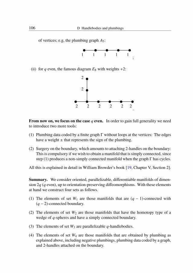
106 D Handlebodies and plumbings
of vertices; e.g, the plumbing graph A5:u u u u u1 1 1 1 1
;
(ii) for q even, the famous diagram E8 with weights +2:
u u u u u u
uu22
2
2
2 2 2 2.
From now on, we focus on the case q even. In order to gain full generality we needto introduce two more tools:
(1) Plumbing data coded by a finite graph Γ without loops at the vertices: The edgeshave a weight ± that represents the sign of the plumbing.
(2) Surgery on the boundary, which amounts to attaching 2-handles on the boundary:This is compulsory if wewish to obtain amanifold that is simply connected, sincestep (1) produces a non-simply connected manifold when the graph Γ has cycles.
All this is explained in detail in William Browder’s book [19, Chapter V, Section 2].
Summary. We consider oriented, parallelizable, differentiable manifolds of dimen-sion 2q (q even), up to orientation-preserving diffeomorphisms. With these elementsat hand we construct four sets as follows.
(1) The elements of set W1 are those manifolds that are (q − 1)-connected with(q − 2)-connected boundary.
(2) The elements of set W2 are those manifolds that have the homotopy type of awedge of q-spheres and have a simply connected boundary.
(3) The elements of set W3 are parallelizable q-handlebodies.
(4) The elements of set W4 are those manifolds that are obtained by plumbing asexplained above, including negative plumbings, plumbing data coded by a graph,and 2-handles attached on the boundary.

D.4 Plumbing 107
Theorem D.13. If q ≥ 4, there is a natural bijection between any two of the sets W1,W2, W3, W4.
Sketch of proof. First we suppose that q is even. We introduce the fifth set S ofisometry classes of symmetric, even bilinear forms on free, finite-dimensional Z-modules.
For each setWi (i = 1, 2, 3, 4) there is a map Ii : Wi −→ S that associates to eachmanifold its intersection form. One proves that each Ii is a bijection (see Browder’sbook [19, Chapter V, Section 2]).
Note on orientations and signs. Let π : E −→ Sq be an orientable q-disc bundleon the sphere Sq . If we choose an orientation b on the base and f on the fiber F, wedefine then an orientation e on E by the rule e = (b, f ) meaning b first and then f .
Note that (b, f ) = ( f , b) if q is even while (b, f ) = −( f , b) if q is odd.LetΦ = (φ1, φ2) be the identification diffeomorphism used for the plumbing, with
diffeomorphisms φ1 : Dq1 −→ ∆
q2 and φ2 : ∆q1 −→ Dq
2 . We denote its action on theorientations by ϕ.
For a positive plumbing we have ϕ(b, f ) = ( f , b) = (b, f ) if q is even; hence Φpreserves the orientations. But we have ϕ(b, f ) = ( f , b) = −(b, f ) if q is odd; henceΦ reverses the orientations. In the latter case, to have an orientation on the manifoldobtained by plumbing we reverse the order (base, fiber) in the second factor. Notethat this depends on the numbering of the factors.
For a negative plumbing, we have ϕ(b, f ) = (− f ,−b) = ( f , b). The conclusion isas above.
In order to compute the intersection between Sq1 and Sq
2 in the plumbed manifoldwe proceed as follows:
• For a positive plumbing we have Sq1 · S
q2 = Sq
1 · Fq1 = +1 in the first factor and
we have Sq1 · S
q2 = Fq
2 · Sq2 = +1 in the second factor. This equality is true
whatever the parity of q is, thanks to the change of orientation for odd q. Thecomputation shows also that the result does not depend on the factor used toperform the computation.
• For a negative plumbing we have Sq1 ·S
q2 = Sq
1 ·(−Fq1 ) = −1 for the computation
with the first factor and Sq1 · S
q2 = (−Fq
2 · Sq2 ) = −1 if we use the second factor
to perform the computation. Hence the intersection number Sq1 ·S
q2 is negative.
Summary. A positive or a negative plumbing preserves the orientations if q is evenand reverses them if q is odd. The intersection number between the spheres is equalto +1 for a positive plumbing and it is equal to −1 for a negative plumbing.


E
Homotopy spheres embedded in codimension 2 and theKervaire–Arf–Robertello–Levine invariant
E.1 Which homotopy spheres can be embedded in codimension 2?
Let Σn be a homotopy sphere differentiably embedded in Sn+2.To answer the question of which homotopy spheres can be embedded in codimen-
sion 2, let us first discuss the case n ≤ 4:
• If n = 1 or 2, there is no problem since Σn = Sn.
• If n = 3, we could invoke Perelman. But there is no need to do that, since Wallproved the lovely result that any 3-manifold embeds differentiably in S5.
• If n = 4, we have to argue a little bit. By Kervaire–Milnor’s [67, Theorem 6.6]we know that every homotopy 4-sphere Σ4 bounds a contractible 5-manifold∆5. Let us take the double of ∆5, i.e., two copies of ∆5 glued along theirboundary. We thus get a homotopy 5-sphere Σ5. But Kervaire–Milnor provedthat any homotopy 5-sphere is diffeomorphic to S5 (see [67, p. 504]). ThereforeΣ4 embeds in S5 and a fortiori in S6.
Note. The arguments for n = 3 and 4 are those of Kervaire in his paper about thegroup of a knot.
Now we consider the set Gn of orientation-preserving diffeomorphism classes oforiented homotopy spheres Σn that can be embedded in Sn+2.
Theorem E.1. Suppose that n ≥ 5.
(1) Then Gn is a finite cyclic group, canonically isomorphic to Z/dn.
(2) If n is even, dn = 1, or in other words Σn = Sn.
(3) Suppose that n is odd, equal to 4k − 1, with k ≥ 2. Then
dn = 22k−2(22k−1 − 1) numerator(
4Bk
k
).
The canonical generator 1 ∈ Z/dn is represented by the boundary of the E8plumbing.

110 E Homotopy spheres and the KARL invariant
(4) If n = 4k + 1 with k ≥ 1, the group Gn is either trivial or isomorphic to Z/2.More precisely,
(41) Gn is trivial if n = 5, 13, 29, 61, and possibly 125 (these are the exceptionalintegers);
(42) Gn is isomorphic to Z/2 if n is not exceptional. The nontrivial element isrepresented by the boundary of the Kervaire plumbing.
The integer dn when n = 4k − 1 was called by Kervaire in a letter to Haefliger“l’entier bordélique bien connu”. The numerator of Bernoulli numbers is indeed atough object, contrary to the denominator.
Items (1), (2), and (3) are an immediate consequence of Kervaire–Milnor, up toa factor 2, which was settled by the solution of the Adams conjecture. Item (4) isintimately related to the Kervaire invariant problem solved in 2009.
The next proposition is the first step towards the proof of the theorem above.
Proposition E.2. A homotopy n-sphere can be embedded differentiably in Sn+2 ifand only if it bounds a parallelizable (n + 1)-manifold.
Sketch of proof. If Σn is embedded in Sn+2 it bounds a Seifert hypersurface, whichis parallelizable since it is orientable and embedded in codimension 1. (Of coursethis argument works with no restriction on n.)
Conversely if Σn bounds abstractly a parallelizable manifold, it also bounds aparallelizable handlebody. Since n ≥ 5, this is true by easy surgery below the middledimension and by the recognition theorem (it is here that (n+1) ≥ 6 is required). It isthen easy to embed such handlebodies in codimension 1. This implies the followingproposition.
Proposition E.3. Let n ≥ 5. The group Gn is isomorphic to Kervaire–Milnor’sgroup bPn+1.
Question. If Σ2q−1 ⊂ S2q+1 is an odd-dimensional knot, can we detect by knotinvariants which homotopy sphere is represented by Σ2q−1?
The answer is yes, and the Seifert form does the work. There are two cases:
(1) If n = 4k − 1 = 2q − 1 (i.e., q is even), the answer is straightforward. Take theSeifert form of any Seifert hypersurface for Σn ⊂ Sn+2, symmetrize it, take thesignature of this bilinear symmetric form (which is the intersection form of thechosen Seifert hypersurface), and divide it by 8. The reduction modulo dn of theinteger so obtained is the element of Z/dn represented by Σn.
(2) If n = 4k + 1 = 2q − 1 (i.e., q is odd), the answer is provided by the Kervaire–Arf–Robertello–Levine invariant as we shall see now.

E.2 The Kervaire–Arf–Robertello–Levine invariant 111
E.2 The Kervaire–Arf–Robertello–Levine invariant
KARL stands for Kervaire, Arf, Robertello, and Levine. They are the main contrib-utors.
The origin of the construction of the KARL invariant goes back to the thesispresented by Kervaire in Paris in June 1964, precisely with the purpose of answeringthe question raised just above. See [64, p. 236]. The study of the invariant was thendeveloped by Robertello in his NYU thesis (Kervaire was the director), also in 1964.See [108]. Soon afterwards, Levine simplified in [79] Robertello’s presentation of theinvariant defined via Seifert forms. In fact, in the case of classical knots Robertellogave two equivalent definitions. One of them can easily apply to higher-dimensionalknots. The data is the following.
We have n = 4k + 1 and K4k+1 ⊂ S4k+3 is a (4k + 1)-dimensional knot, whereK4k+1 is diffeomorphic to the homotopy sphere Σ4k+1. The case n = 1 (i.e., k = 0)is admitted. Let F4k+2 be a Seifert hypersurface for K4k+1.
We denote by H the quotient of H2k+1(F; Z) by its Z-torsion subgroup. LetA : H × H → Z be the Seifert form defined by A(x, y) = Lk(x; i+y).Definition E.4. We define the quadratic form QF : H ⊗ Z/2 → Z/2 by QF (x) =Lk2(x; i+(x)), where Lk2 denotes the linking number reduced mod 2.Lemma E.5. We have the equality QF (x + y) = QF (x) + QF (y) + x · y where x · ydenotes the intersection number in F reduced mod 2.
We denote by Arf(QF ) the Arf invariant of the quadratic form QF . Note that thebilinear form (x, y) 7→ x · y is unimodular, since ∂F is a homotopy sphere.Theorem E.6 (Robertello; Levine [79]). Arf(QF ) is a knot invariant, i.e., it does notdepend on the choice of a Seifert hypersurface.
Sketch of Levine’s proof. Let p : E(K) → E(K) be the infinite cyclic covering ofthe knot complement E(K) = S4k+3 \ N(K). Let ∆K (t) ∈ Z[t, t−1] be the Alexanderpolynomial of the knot module H2k+1(E(K); Q) normalized à la Conway by ∆(t−1) =∆(t) and ∆(1) = 1. Then Levine proves that ∆(−1) ≡ 1+4 Arf(QF ) mod 8. (Levine’sproof is a beauty.)
DefinitionE.7. Wedefine theKARL invariantKARL(K) of the knotK to beArf(QF )
for any Seifert hypersurface F.Theorem E.8 (Robertello; Levine). KARL(K) is a knot cobordism invariant.Sketch of proof, following Levine. By Levine [80], the Fox–Milnor result is true inhigher dimensions. More precisely, if K is cobordant to zero, there exists an elementP(t) ∈ Z[t, t−1] such that ∆(t) = P(t)P(1/t). Since ∆(1) = 1 we deduce that P(−1)is odd and hence ∆(−1) is an odd square and therefore congruent to 1 mod 8. HenceKARL(K) = 0 if K is cobordant to zero.

112 E Homotopy spheres and the KARL invariant
E.3 The Hill–Hopkins–Ravenel result and its influence on the KARLinvariant
Theorem E.9 (Browder [18] and Hill–Hopkins–Ravenel [47]). The “boundary”homomorphism
b : P4k+2 = Z/2→ Θ4k+1
is trivial if 4k + 2 = 2, 6, 14, 30, 62, and possibly 126. (These are the exceptionalintegers +1.)
In all other cases it is injective and hence bP4k+2 = Z/2.
Theorem E.10. If (4k + 1) is not exceptional, the Arf invariant of the quadraticform defined via the Seifert form (i.e., the KARL invariant of the knot) detects whichhomotopy sphere of dimension 4k + 1 is embedded.
Proof of Theorem E.9. Let us first suppose that the knot K4k+1 is simple. Let F4k+2
be a 2k-connected Seifert hypersurface. Hence the quadratic form H2k+1(F; Z/2) →Z/2 “à la Kervaire–Milnor” is defined (see [72, pp. 202–207]).
By [68, lemma on normal bundles, p. 512], this last quadratic form coincides withthe quadratic form that gives rise to the KARL invariant. Hence KARL(K) detectswhich element of P4k+2 is represented by F4k+2 and hence which element of bP4k+2
is represented by K4k+1.Let us now withdraw the assumption that K is simple. We know that its KARL
invariant is defined. By [80] there exists a simple knot K∗ that is knot-cobordantto K . By [79] the knots K and K∗ have the same KARL invariant. Since K andK∗ are diffeomorphic, KARL(K∗) = KARL(K) detects which element of bP4k+2 isrepresented by K .
Recap. In terms of bP4k+2 the interpretation of the KARL invariant splits into twocases.
(i) If bP4k+2 = Z/2 there are two homotopy spheres of dimension (4k +1) that canbe embedded in S4k+3 to represent knots. The KARL invariant detects whichhomotopy sphere it is. Thus the differential structure on the homotopy sphereis detected by the Alexander module (in dimension (2k + 1)) of the knot. Inother words, different differential structures give rise to different knot modulesin dimension (2k + 1).
Caution. The KARL invariant detects the Arf invariant of the handlebody (i.e.,of the Seifert hypersurface). If you know beforehand that the Kervaire invariant isnontrivial, then it detects which homotopy sphere is represented by the boundary ofthe handlebody.
E.3 The Hill–Hopkins–Ravenel result and the KARL invariant 113
(ii) If bP4k+2 = 0, all (4k + 1)-knots are represented by an embedding of thestandard sphere. From a knot theory point of view, one could argue that thissituation is more interesting, since the KARL invariant is a genuine invariantof the embedding. The case of classical knots is typical.
An (easy) consequence of our discussion of the KARL invariant produces a proofof the following result, when n = 4k + 1. If n = 4k + 3, it can be obtained by usingthe signature and Blanchfield duality. See Dieter Erle [33].
Theorem E.11. Let n ≥ 5. Let Σn and Σn be homotopy spheres embedded in Sn+2.Suppose that the two homotopy spheres are not diffeomorphic. Then the two knotsare not topologically isotopic.


F
Figures
In this chapter we propose a few figures to help to visualize some concepts. We findit useful to gather the figures together in the same place, since the related conceptsare spread out in the text.
In Appendix A, we presented the general conventions for orientation and signthat we have followed throughout the book. These are valid in any dimension. InFigures F.1, F.2, and F.3 we show what we consider to be the standard orientations ofthe 2-plane and 3-space. This enables us to ascribe a sign to some objects representedin the pictures. We are aware that these conventions in small dimensions are subjectto controversy.
e
e
1
2
Figure F.1. S1 is oriented as the boundary of B2. In the figure the frame (e1, e2) represents ourstandard orientation of the plane.
e e
e
1
2
3
Figure F.2. Space orientation braid representation of a Hopf link. If oriented as a closed braid,the linking coefficient between the two components is equal to +1, since the frame (e1, e2, e3)corresponds to the three fingers of the right hand: (thumb, forefinger, middle finger). The frame isobtained as follows. The vectors (e1, e2) are tangent to the 2-disc spanned by the component that ison the right. The vector e3 is tangent to the component that is on the left.
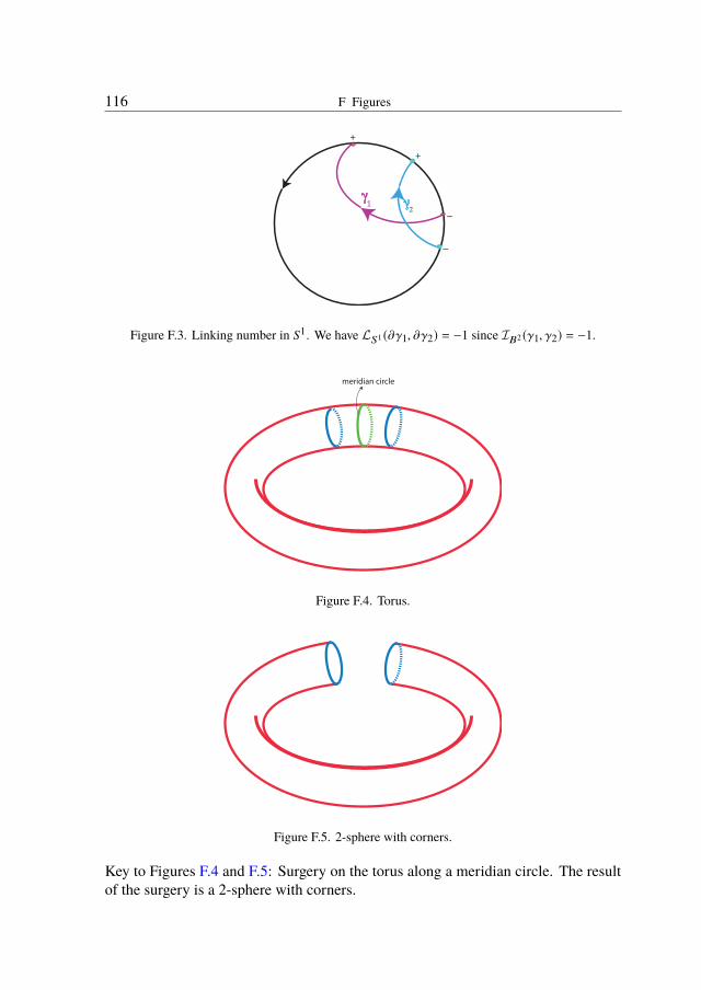
116 F Figures
2
+
_
+
_
Figure F.3. Linking number in S1. We have LS1 (∂γ1, ∂γ2) = −1 since IB2 (γ1, γ2) = −1.
meridian circle
Figure F.4. Torus.
Figure F.5. 2-sphere with corners.
Key to Figures F.4 and F.5: Surgery on the torus along a meridian circle. The resultof the surgery is a 2-sphere with corners.

F Figures 117
Figure F.6. Seifert surface for the Hopf link represented in Figure F.2.
Figure F.7. Seifert surface for a trefoil knot presented as a 1-handlebody in 3-space.
aa1
21e
2e
Figure F.8. How to obtain the Seifert form of the trefoil of Figure F.7.
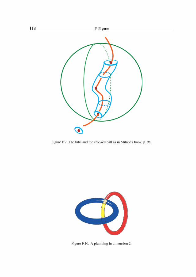
118 F Figures
Figure F.9. The tube and the crooked ball as in Milnor’s book, p. 98.
Figure F.10. A plumbing in dimension 2.

F Figures 119
Figure F.11. One of the two possible parallelizable 1-handlebodies with two handles.
Figure F.12. The other of the two possible parallelizable 1-handlebodies with two handles.


Bibliography
[1] Norbert A’Campo: “Le nombre de Lefschetz d’une monodromie”, Indag. Math. 35 (1973)113–118. Zbl 0276.14004.
[2] Norbert A’Campo: “La fonction zêta d’une monodromie”, Comment. Math. Helv. 50 (1975)233–248. Zbl 0333.14008.
[3] John Frank Adams: “On the groups J(X)-II”, Topology 3 (1965) 137–171. Zbl 0137.16801.
[4] John Frank Adams: “On the groups J(X)-IV”, Topology 5 (1965) 21–71. Zbl 0145.19902.
[5] John Frank Adams: “Algebraic topology in the last decade”, in AMS Proc. Symp. Pure Math.22 (1971) 1–22. Zbl 0235.55001.
[6] Enrique Artal Bartolo: “Forme de Seifert des singularités de surface”, Comptes-Rendus del’Académie des Sciences de Paris 313 (1991) 689–692. Zbl 0746.32012.
[7] Michael Atiyah and Friedrich Hirzebruch: “Riemann-Roch theorems for differentiable man-ifolds”, Bull. Amer. Math. Soc. 65 (1959) 276–281. Zbl 0142.40901.
[8] Michael Barratt, John Jones and Mark Mahowald: “The Kervaire invariant problem”, inProc. Northwestern Homotopy Theory Conference, Contemporary Math. AMS 19 (1983)9–22. Zbl 0528.55010.
[9] Available at www.bernoulli.org.
[10] Vincent Blanloeil and Françoise Michel: “A theory of cobordism for non-spherical links”,Comment. Math. Helv. 72 (1997) 30–51. Zbl 0893.57023.
[11] Philippe du Bois and Françoise Michel: “Cobordism of algebraic knots via Seifert forms”,Invent. Math. 111 (1993) 151–169. Zbl 0789.57015.
[12] Philippe du Bois and Françoise Michel: “The integral Seifert form does not determine thetopology of plane curve germs”, J. Algebraic Geom. 3 (1994) 1–38. Zbl 0810.32005.
[13] Raoul Bott: “The stable homotopy of the classical groups”, Annals of Math. 70 (1959)313–337. Zbl 0129.15601.
[14] Raoul Bott and John Milnor: “On the parallelizability of the spheres”, Bull. Amer. Math.Soc. 64 (1958) 87–89. Zbl 0082.16602.
[15] Egbert Brieskorn: “Beispiele zur Differentialtopologie von Singularitäten”, Invent. Math. 2(1966) 1–14. Zbl 0145.17804.
[16] Egbert Brieskorn: “Singularities in the work of Friedrich Hirzebruch”, Surveys in Differen-tial Geometry VII (2000) 17–60. Zbl 1084.32506.
[17] William Browder: “Diffeomorphisms of 1-connected manifolds”, Trans. Amer. Math. Soc.128 (1967) 155–163. Zbl 0166.19702.
[18] William Browder: “The Kervaire invariant of framed manifolds and its generalization”,Annals of Math. 90 (1969) 157–186. Zbl 0198.28501.

122 Bibliography
[19] William Browder: Surgery on Simply-Connected Manifolds, Springer (1972).Zbl 0239.57016.
[20] Edgar Brown Jr and Frank Peterson: “The Kervaire invariant of (8k + 2)-manifolds”, Amer.J. Math. 88 (1966) 815–826. Zbl 0148.17401.
[21] Greg Brumfiel: “On the homotopy groups of BPL and of PL/O”, Annals of Math. 88 (1968)291–311. Zbl 0162.27302.
[22] Gerhard Burde and Heiner Zieschang: “Eine Kennzeichnung der Torusknoten”, Math.Annalen 167 (1966) 169–176. Zbl 0145.20502.
[23] Sylvain Cappell and Julius Shaneson: “There exist inequivalent knots with the same com-plement”, Annals of Math. 103 (1976) 349–353. Zbl 0338.57008.
[24] Sylvain Cappell and Julius Shaneson: “Some new four manifolds”, Annals of Math. 104(1976) 61–72. Zbl 0345.57003.
[25] Jean Cerf: “Topologie de certains espaces de plongements”, Bull. Soc. Math. France 89(1961) 227–380. Zbl 0101.16001.
[26] Jean Cerf: Sur les difféomorphismes de la sphère de dimension trois (Γ4 = 0), SpringerLecture Notes 53 (1968). Zbl 0164.24502.
[27] Jean Cerf: “La stratification naturelle des espaces de fonctions différentiables réelles etthéorème de la pseudo-isotopie”, Publ. Math. IHES 39 (1970) 5–173. Zbl 0213.25202.
[28] Lawrence Conlon: Differentiable Manifolds: A First Course, Birkäuser (1993).Zbl 0770.57001.
[29] Alan Durfee: “Fibered knots and algebraic singularities”, Topology 13 (1974) 47–59.Zbl 0275.57007.
[30] Alan Durfee: “Singularities” in History of Topology, I. M. James (ed.), North HollandAmsterdam (1999) 417–434. Zbl 0956.57003.
[31] Eldon Dyer and Alphonse Vasquez: “The sphericity of higher dimensional knots”, Canad.J. Math. 25 (1973) 1132–1136. Zbl 0275.57006.
[32] Samuel Eilenberg and Norman Steenrod: Foundations of Algebraic Topology, PrincetonUniversity Press (1952). Zbl 0047.41402.
[33] Dieter Erle: “Smooth structures and signatures of codimension two embeddings”, Proc.Amer. Math. Soc. 35 (1972) 611–616. Zbl 0251.57010.
[34] Michael Farber: “An algebraic classification of some even-dimension spherical knots I andII”, Trans. Amer. Math. Soc. 281 (1984) 507–527 and 529–570. Zbl 0536.57010.
[35] Roger Fenn and Colin Rourke: “Klyachko’s methods and the solution of equations overtorsion-free groups”, L’Ens. Math. 42 (1996) 49–74. Zbl 0861.20029.
[36] Michael Freedman: “The topology of four-dimensional manifolds”, J. Differential Geom.17 (1982) 357–453. Zbl 0528.57011.
[37] Herman Gluck: ‘The embedding of two-spheres in the four-sphere”, Bull. Amer. Math. Soc.67 (1961) 586–589. Zbl 0173.51402.

Bibliography 123
[38] Cameron Gordon: “Some aspects of classical knot theory”, in Knot Theory, Proc. Semin.Plans-sur-Bex (1977), Springer Lecture Notes 685 (1978) 1–60. Zbl 0386.57002.
[39] Cameron Gordon and John Luecke: “Knots are determined by their complements”, J. Amer.Math. Soc. 2 (1989) 371–415. Zbl 0678.57005.
[40] Maurizio Gutierrez: “On knot modules”, Inventiones Math. 17 (1972) 329–335.Zbl 0243.57007.
[41] André Haefliger: “Differentiable imbeddings”, Bull. Amer. Math. Soc. 67 (1961) 109–112.Zbl 0099.18101.
[42] André Haefliger: “Differentiable links”, Topology 1 (1962) 241–244. Zbl 0108.18201.
[43] André Haefliger: “Knotted (4k − 1)-spheres in 6k-space”, Annals of Math. 75 (1962) 452–466. Zbl 0105.17407.
[44] André Haefliger: Sphères d’homotopie nouées, Séminaire Bourbaki 280 (1964/65).Zbl 0196.55904.
[45] Jean-Claude Hausmann and Michel Kervaire: “Sous-groupes dérivés des groupes denoeuds”, L’Ens. Math. 24 (1978) 111–123. Zbl 0414.57012.
[46] Jean-Claude Hausmann andMichel Kervaire: “Sur le centre des groupes de noeuds multidi-mensionnels”, Comptes-Rendus de l’Académie des Sciences de Paris 287 (1978) 699–702.Zbl 0397.57004.
[47] Mike Hill, Mike Hopkins, and Doug Ravenel: “On the nonexistence of elements of theKervaire invariant one”, Annals of Math. (2) 184 (2016) 1–262 (2016). Zbl 06605831.
[48] Jonathan Hillman: 2-Knots and Their Groups, Australian Math. Soc. Lecture Series 5(1989). Zbl 0669.57008.
[49] Morris Hirsch: Differential Topology, Graduate Texts in Mathematics, Springer (1976).Zbl 0356.57001.
[50] Morris Hirsch and Lee Neuwirth: “On piecewise regular n-knots”, Annals of Math. 80(1964) 594–612. Zbl 0168.21601.
[51] Friedrich Hirzebruch: “Über vierdimensionale Riemannsche Flächen mehrdeutiger ana-lytischer Funktionen von zwei komplexen Veränderlichen”,Math. Annalen 126 (1953) 1–22.Zbl 0093.27605.
[52] Friedrich Hirzebruch: Topological Methods in Algebraic Geometry, Springer (1966).Zbl 0138.42001.
[53] Friedrich Hirzebruch and Karl Heinz Mayer: O(n)-Mannigfaltigkeiten, exotische Sphärenund Singularitäten, Springer Lecture Notes 57 (1968). Zbl 0172.25304.
[54] Klaus Johannson: Homotopy Equivalences of 3-Manifolds with Boundaries, Springer Lec-ture Notes 761 (1979). Zbl 0412.57007.
[55] Mitsuyoshi Kato: “A classification of simple spinnable structures on a 1-connected Alexan-der manifold”, J. Math. Soc. Japan 3 (1974) 454–463. Zbl 0288.57013.

124 Bibliography
[56] Louis Kauffman: “Branched coverings, open books and knot periodicity”, Topology 13(1974) 143–160. Zbl 0283.57011.
[57] Louis Kauffman and Walter Neumann: “Product of knots, branched coverings and sums ofsingularities”, Topology 16 (1977) 369–393. Zbl 0447.57012.
[58] Cherry Kearton: “An algebraic classification of certain simple even-dimensional knots”,Trans. Amer. Math. Soc. 276 (1983) 1–53. Zbl 0508.57013.
[59] Michel Kervaire: “Courbure intégrale géneralisée et homotopie”,Math. Annalen 131 (1956)219–252. Zbl 0072.18202.
[60] MichelKervaire: “Non-parallelizability of the n-sphere for n > 7”,Proc. Nat. Acad. Sciences44 (1958) 280–283. Zbl 0093.37303.
[61] Michel Kervaire: “An interpretation of G. Whitehead’s generalization of H. Hopf’s invari-ant”, Annals of Math. (2) 69 (1959) 345–365. Zbl 0088.39205.
[62] Michel Kervaire: “Amanifold which does not admit any differentiable structure”, Comment.Math. Helv. 34 (1960) 257–270. Zbl 0145.20304.
[63] Michel Kervaire: “On knots in higher dimensions”, in Differential and CombinatorialTopology, A Symposium in Honor of Marston Morse (1963). Princeton University Press(1965) 105–119. Zbl 0134.42903.
[64] Michel Kervaire: “Les noeuds de dimensions supérieures”, Bull. Soc. Math. France 93(1965) 225–271. Zbl 0141.21201.
[65] Michel Kervaire: “Smooth homology spheres and their fundamental groups”, Trans. Amer.Math. Soc. 144 (1969) 67–72. Zbl 0187.20401.
[66] Michel Kervaire: “Knot cobordism in codimension two”, in Manifolds - Amsterdam 1970,Proc. NUFFIC Summer School, Springer Lecture Notes in Math. 197 (1970) 83–105.Zbl 0225.57006.
[67] Michel Kervaire and John Milnor: “Groups of homotopy spheres”, Annals of Math. 77(1963) 504–537. Zbl 0115.40505.
[68] Michel Kervaire and Alphonse Vasquez: “Simple connectivity and the Browder-Novikovtheorem”, Trans. Amer. Math. Soc. 126 (1967) 508–513. Zbl 0173.26103.
[69] Michel Kervaire and Claude Weber: “A survey of multidimensional knots”, in KnotTheory, Proc. Semin. Plans-sur-Bex (1977), Springer Lecture Notes 685 (1978) 61–134.Zbl 0386.57011.
[70] Alexander Klyachko: “A funny property of sphere and equations over groups”, Comm.Algebra 21 (1993) 2555–2575. Zbl 0788.20017.
[71] Sadayoshi Kojima: “Classification of simple knots by Levine pairings”, Comment. Math.Helv. 54 (1979) 356–367. Zbl 0417.57008.
[72] Antoni Kosinski: Differential Manifolds, Dover Publications (1993). Zbl 0767.57001.
[73] Richard Lashof and Julius Shaneson: “Classification of knots in codimension two”, Bull.Amer. Math. Soc. 75 (1969) 171–175. Zbl 0198.28701.

Bibliography 125
[74] Lê Dung Tráng: “Sur les noeuds algébriques”, Compositio Math. 25 (1972) 281–321.Zbl 0245.14003.
[75] Lê Dung Tráng: “La monodromie n’a pas de points fixes”, J. Fac. Sci. Univ. Tokyo 22 (1975)409–427. Zbl 0355.32012.
[76] Lê Dung Tráng and Bernard Perron: “Sur la fibre de Milnor d’une singularité isolée endimension complexe trois”, Comptes-Rendus de l’Académie des Sciences de Paris 289(1979) 115–118. Zbl 0451.32007.
[77] Jerome Levine: “Unknotting spheres in codimension two”, Topology 4 (1965) 9–16.Zbl 0134.42803.
[78] Jerome Levine: “A classification of differentiable knots”, Annals of Math. 82 (1965) 15–50.Zbl 0136.21102.
[79] Jerome Levine: “Polynomial invariants of knots of codimension two”, Annals of Math. 84(1966) 537–544. Zbl 0196.55905.
[80] Jerome Levine: “Knot cobordism groups in codimension two”, Comment. Math. Helv. 44(1969) 229–244. Zbl 0176.22101.
[81] Jerome Levine: “An algebraic classification of some knots of codimension two”, Comment.Math. Helv. 45 (1970) 185–198. Zbl 0211.55902.
[82] Jerome Levine: “Knot modules I”, Trans. Amer. Math. Soc. 229 (1977) 1–50.Zbl 0653.57012.
[83] Jerome Levine: “Some results on higher dimension knot groups”, in Knot Theory, Proc.Semin. Plans-sur-Bex (1977), Springer Lecture Notes 685 (1978) 243–273. Zbl 0404.57019.
[84] Jerome Levine: “Lectures on groups of homotopy spheres”, in Algebraic and Geomet-ric Topology (New Brunswick, NJ, 1983), Springer Lecture Notes 1126 (1985) 62–95.Zbl 0576.57028.
[85] Saunders Mac Lane: Homology, Springer (1963). Zbl 0133.26502.
[86] Mark Mahowald and Martin Tangora: “Some differentials in the Adams spectral sequence”,Topology 6 (1967) 349–369. Zbl 0166.19004.
[87] Françoise Michel: “Formes de Seifert et singularités isolées”, in Noeuds, tresses et sin-gularités (Semin. Plans-sur-Bex 1982), Monographie de l’Enseignement Mathématique 31(1983) 175–190. Zbl 0557.57014.
[88] John Milnor: “Construction of universal bundles. II”, Annals of Math. 63 (1956) 430–436.Zbl 0071.17401.
[89] John Milnor: “Differentiable manifolds which are homotopy spheres”, Multicopied notes(1959). Zbl 0106.37001.
[90] John Milnor: “Sommes de variétés différentiables et structures différentiables des sphères”,Bull. Soc. Math. France 87 (1959) 439–444. Zbl 0096.17801.
[91] John Milnor: “A procedure for killing homotopy groups of differentiable manifolds”, AMSProc. Symp. Pure Math. 3 (1961) 39–55. Zbl 0118.18601.
126 Bibliography
[92] John Milnor: “Differential topology”, in Lectures on Modern Mathematic Vol. II, T.L. Saaty(ed.) (1964) 165–183. Zbl 0123.16201.
[93] JohnMilnor: Singular Points of Complex Hypersurfaces, Annals of Math. Studies 61 (1968)Princeton University Press. Zbl 0184.48405.
[94] John Milnor and Michel Kervaire: “Bernoulli numbers, homotopy groups and a theorem ofRohlin”, in Proc. Int. Congress of Math. Edinburgh, 1958 (1960) 454–458. Zbl 0119.38503.
[95] John Milnor and James Stasheff: Lectures on Characteristic Classes, Annals of Math.Studies 76 (1974). Zbl 0298.57008.
[96] Edwin Moise: “Affine structures in 3-manifolds. V: The triangulation theorem and theHauptvermutung”, Annals of Math. 57 (1952) 96–114. Zbl 0048.17102.
[97] David Mumford: “The topology of normal singularities of an algebraic surface and acriterion for simplicity”, J. IHES, Publ. Math. 9 (1961) 5–22. Zbl 0108.16801.
[98] James Munkres: “Obstructions to the smoothing of piece-wise differentiable homeomor-phisms”, Annals of Math. 72 (1960) 321–354. Zbl 0108.18101.
[99] Walter Neumann: “A calculus for plumbing applied to the topology of complex surfacesingularities and degenerating complex curves”, Trans. Amer. Math. Soc. 268 (1981) 299–343. Zbl 0546.57002.
[100] Lee Neuwirth: Knot Groups, Annals of Math. Studies 56 (1965) Princeton University Press.Zbl 0184.48903.
[101] Maxwell Newman: “The engulfing theorem for topological manifolds”, Annals of Math. 84(1966) 555–571. Zbl 0166.19801.
[102] Christos Papakyriakopoulos: “On Dehn’s lemma and the asphericity of knots”, Annals ofMath. 66 (1957) 1–26. Zbl 0078.16402.
[103] Lev Pontrjagin: “Classification homotopique des applications de la sphère à (n+2) dimen-sions sur celle à n dimension”, C. R. Acad. Sci. URSS 70 (1950) 957–959 (in Russian).Zbl 0035.11101.
[104] Lev Pontrjagin: “Smooth manifolds and their applications in homotopy theory”, in Russian:Trudy Mat. Inst. im Steklov 45 (1955); translation in English: Amer. Math. Soc. Translations11 (1959) 1–114. Zbl 0064.17402.
[105] Andrew Ranicki: High Dimensional Knot Theory. Algebraic Surgery in Codimension 2,Springer Monographs in Mathematics (1998). Zbl 0910.57001.
[106] AndrewRanicki: “Blanchfield and Seifert algebra in high dimensional knot theory”,MoscowMath. J. 3 (2003) 1333–1367. Zbl 1059.19003.
[107] Douglas Ravenel: Complex Cobordism and Stable Homotopy Groups of Spheres, ChelseaPublishing Company AMS 347 (2004). Zbl 1073.55001.
[108] Raymond Robertello: “An invariant of knot cobordism”, Comment. Pure and Applied Math.18 (1965) 543–555. Zbl 0151.32501.
[109] Koichi Sakamoto: “The Seifert matrices of Milnor fiberings defined by holomorphic func-tions”, J. Math. Soc. Japan 26 (1974) 714–721. Zbl 0286.32010.
Bibliography 127
[110] Marcos Sebastiani and René Thom: “Un résultat sur la monodromie”, Invent. Math. 13(1971) 90–96. Zbl 0233.32025.
[111] Herbert Seifert and William Threlfall: Lehrbuch der Topologie, Teubner (1934).Zbl 0009.08601.
[112] Jean-Pierre Serre: “Homologie singulière des espaces fibrés”, Annals of Math. 54 (1951)425–505. Zbl 0045.26003.
[113] Arnold Shapiro: “Obstructions to the embedding of a complex in Euclidean space. I Thefirst obstruction”, Annals of Math. 66 (1957) 256–269. Zbl 0085.37701.
[114] Daniel Silver, Wilbur Whitten, and Susan Wiliams: “Knot groups with many killers”, Bull.Australian Math. Soc. 81 (2010) 507–513. Zbl 1194.57013.
[115] Stephen Smale: “Diffeomorphisms of the 2-sphere”, Proc. Amer. Math. Soc. 10 (1959)621–626. Zbl 0118.39103.
[116] Stephen Smale: “The generalized Poincaré conjecture in higher dimensions”, Bull. Amer.Math. Soc. 66 (1960) 373–375. Zbl 0099.39201.
[117] Stephen Smale: “On the structure of manifolds”, Amer. J. Math. 84 (1962) 387–399.Zbl 0109.41103.
[118] John Stallings: “Polyhedral homotopy spheres”, Bull. Amer. Math. Soc. 66 (1960) 485–488.Zbl 0111.18901.
[119] John Stallings: “On topologically unknotted spheres”, Annals of Math. 77 (1963) 490–503.Zbl 0121.18202.
[120] Norman Steenrod: The Topology of Fibre Bundles Princeton University Press (1951).Zbl 0054.07103.
[121] Eduard Stiefel: “Richtungsfelder und Fernparallelismus in n-dimensionen Mannig-faltigkeiten”, Comment. Math. Helv. 8 (1936) 305–353. Zbl 0014.41601.
[122] Neal Stoltzfus: “Unraveling the integral knot concordance group”, Mem. Amer. Math. Soc.192 (1977). Zbl 0366.57005.
[123] Richard Swan: “Projective modules over Laurent polynomial rings”, Trans. Amer. Math.Soc. 237 (1978) 111–120. Zbl 0404.13006.
[124] René Thom: “Quelques propriétés globales des variétés différentiables”, Comment. Math.Helv. 29 (1954) 17–86. Zbl 0057.15502.
[125] Hale Trotter: “On S-equivalence of Seifert matrices”, Invent. Math. 20 (1973) 173–207.Zbl 0269.15009.
[126] Friedhelm Waldhausen: “On irreducible 3-manifolds which are sufficiently large”, Annalsof Math. 87 (1968) 56–88. Zbl 0157.30603.
[127] C.T.C. Wall: “Classification of (n− 1)-connected 2n-manifolds”, Annals of Math. 75 (1962)163–189. Zbl 0218.57022.
[128] C.T.C. Wall: “Classification problems in differential topology I”, Topology 2 (1963) 253–261. Zbl 0123.16203.

128 Bibliography
[129] C.T.C. Wall: “Classification problems in differential topology II”, Topology 2 (1963) 263–272. Zbl 0123.16204.
[130] C.T.C.Wall: “On simply-connected 4-manifolds”, J. LondonMath. Soc. 39 (1964) 141–149.Zbl 0131.20701.
[131] C.T.C. Wall: “Classification problems in differential topology III”, Topology 3 (1965) 291–304. Zbl 0141.21101.
[132] C.T.C. Wall: “Classification problems in differential topology VI. Classification of (s − 1)-connected (2s + 1)-manifolds”, Topology 6 (1967) 273–296. Zbl 0173.26102.
[133] C.T.C. Wall: Surgery on Compact Manifolds, London Math. Soc. Monographs AcademicPress (1970). Zbl 0219.57024.
[134] Hassler Whitney: “Differentiable manifolds”, Annals of Math. 37 (1936) 645–680.Zbl 0015.32001.
[135] Hassler Whitney: “The self-intersections of a smooth n-manifold in 2n-space”, Annals ofMath. 45 (1944) 220–246. Zbl 0063.08237.
[136] Christopher Zeeman: “Knotting manifolds”, Bull. Amer. Math. Soc. 67 (1961) 117–119.Zbl 0126.18903.
[137] Christopher Zeeman: “Unknotting combinatorial balls”, Annals of Math. 78 (1963) 501–526. Zbl 0122.17901.

Index of Notation
Bn+1 standard ball of dimension (n + 1) 9
Bn+1 standard open ball of dimension (n + 1) 9
bPn+1 group of homotopy n-spheres that bound parallelizable manifolds 18
C2q cobordism group of 2q-dimensional knots 69
C2q−1 cobordism group of (2q − 1)-dimensional knots 71
Cε cobordism group of ε-forms 72
Γn group of twisted n-spheres 19
Λn set of oriented homotopy n-spheres 15
Pn+1 Kervaire–Milnor framed cobordism group 22
Sn standard n-sphere 9
Θn h-cobordism group of oriented homotopy n-spheres 16


Index of Quoted Theorems
Adams theorem on the stable J-homomorphism 13
Bott periodicity theorem 13
Brieskorn theorem on Pham–Brieskorn singularities 5
Haefliger theorem on differentiable knots of S4k−1 in S6k 29
Haefliger theorem on embeddings in the metastable range 29
Haefliger theorem on m-dimensional spherical links in S2m+1 103
Hill–Hopkins–Ravenel theorem on the Kervaire invariant 22, 112
Hopf theorem on H2(Γ) 36
Kervaire’s conditions on a knot group 35
Kervaire theorem on the realizabilty of his conditions on a knot group 38
Kervaire theorem on knot modules 48
Kervaire–Milnor main theorem on Θn 17
Kervaire–Milnor theorem on bPn+1 18
Kervaire–Milnor’s computation of Pn+1 23
Levine unknotting theorem 43
Levine theorem on S-equivalence for simple knots 67
Levine theorem on the algebraic characterization of the 73knot-cobordism group
Milnor fibration theorem 76
Mumford theorem on singularities of complex algebraic surfaces 81
Pontrjagin isomorphism theorem 12

132 Index of Quoted Theorems
Realization theorem of Seifert matrices 62
Recognition theorem of q-handlebodies 100
Silver–Whitten–Williams theorem on killers in a knot group 36
Whitehead theorem on the homotopy type of C.W. complexes 43
Whitney theorem on embeddings in the stable range 28

Index of Terminology
algebraic link, 79almost parallelizable manifold, 16Arf invariant, 21aspherical C.W. complex, 43attaching link, 61, 99
Bernoulli number Bk , 13binding (of an open book
decomposition), 76, 95Bott periodicity, 13
classical knot, 33closed manifold, 7cobordant ε-forms, 72cobordant knots, 69codimension of a link, 3common part of a surgery, 9core, 61, 99
ε-form, 72exterior of a knot, 1, 33exterior of a submanifold, 7
framed manifold, 12framed cobordant manifolds, 12framed cobordism, 23
group of a knot, 4group of a link, 4
h-cobordant manifolds, 29handle of index q, 99handle presentation, 61, 99handlebody, q-handlebody, 24, 61, 99homotopy sphere, 15
intersection number, 92
join (of two compact spaces), 85
Kervaire–Arf–Robertello–Levineinvariant, 111
Kervaire conjecture, 40Kervaire invariant, 21Kervaire manifold, 25Kervaire’s Paris paper, 1knot, 1knot manifold, 37knot module, 44
link of a germ, 75link, n-link in codimension q, 3linking number, 92
m-spherical r-link in S2m+1, 103mapping cylinder, 85mapping torus, 76, 95meridian of a knot, 36meridian of a link, 93metabolizer of an ε-form, 72Milnor fiber, 75minimal (Seifert hypersurface), 52module of type K, 46monodromy, 76
n-knot in codimension q, 4, 27null-cobordant ε-form, 72null-cobordant knot, 69
open book decomposition, 76, 95ordinary double point, 83
page (of an open book decomposition),76
parallelizable manifold, 10Pham–Brieskorn singularity, 83plumbing, 104Pontrjagin construction, 12
134 Index of Terminology
rank of a vector bundle, 7
S-equivalent (Seifert forms), 55scars of a surgery, 9Seifert form, 53Seifert hypersurface of a link, 4, 93Seifert hypersurface of a knot, 34, 50(2q − 1)-simple fibered link, 77(2q − 1)-simple link, 61simple n-knot, 52skeleton (of a q-handlebody), 61slice knot, 69stable homotopy group of spheres, 12stable J-homomorphism, 13stably parallelizable manifold, 10stably trivial vector bundle, 10standard ball, 9standard n-knot, 33standard sphere, 9surgery, 9
topological type (of a germ), 75topologically trivial germ, 82torsion linking forms, 57torsion Seifert forms, 58trivial vector bundle, 10
weight (of a group), 35

Series of Lectures in Mathematics
Michel/Weber | Rotis Sans | Pantone 287, Pantone 116 | 170 x 240 mm | RB: 7.2 mm
Françoise MichelClaude Weber
Higher-Dimensional Knots According to Michel Kervaire
Michel Kervaire wrote six papers on higher-dimensional knots which can be considered fundamental to the development of the theory. They are not only of historical interest but naturally introduce to some of the essential techniques in this fascinating area.
This book is written to provide graduate students with the basic concepts necessary to read texts in higher-dimensional knot theory and its relations with singularities. The first chapters are devoted to a presentation of Pontrjagin’s construction, surgery and the work of Kervaire and Milnor on homotopy spheres. We pursue with Kervaire’s fundamental work on the group of a knot, knot modules and knot cobordism. We add developments due to Levine. Tools (like open books, handlebodies, plumbings, …) often used but hard to find in original articles are presented in appendices. We conclude with a description of the Kervaire invariant and the consequences of the Hill–Hopkins–Ravenel results in knot theory.
ISBN 978-3-03719-180-4
www.ems-ph.org
Françoise Michel and Claude W
eberH
igher-Dimensional Knots According to M
ichel Kervaire
Françoise MichelClaude Weber
Higher-Dimensional Knots According to Michel Kervaire