high strain rate testing and modeling of polymers for...

HIGH STRAIN RATE TESTING AND MODELING OF POLYMERS FOR USE IN

FINITE ELEMENT SIMULATIONS

Sean S. Teller, Jorgen S. Bergström, Gregory R. Freeburn, Veryst Engineering, Needham, MA

Abstract

Finite element analysis plays a crucial role in modern

engineering problems, enabling engineers to predict the

response of designed parts at any point in the design

process. Specifying a constitutive model that accurately

captures the mechanical response of a polymer material is

paramount to obtaining useful results. In order to

understand the capabilities of commercial FE packages

used to simulate problems involving polymers, we have

tested the uniaxial response of polyamide in tension and

compression over six decades of strain rate. We then

calibrated four constitutive models to the experimental

data: an Abaqus Parallel Rheological Framework model,

the LS-DYNA SAMP-1 model, the ANSYS Bergström-

Boyce model, and the PolyUMod Three Network model.

We compared the performance of the four models in

predicting the experimental data; the Three Network

model had the lowest error. Additionally, we compared

the runtime of a simple test case for each model; the

ANSYS Bergström-Boyce model being the fastest.

Introduction

The Finite Element (FE) method is an important and

widely used tool to design and analyze the response of

solid parts to real world loading conditions [1]. Accurate

specification of the constitutive model is important to

obtain applicable results. Polymers exhibit complex

mechanical behavior, including plastic flow, viscoelastic

flow, hysteresis, and strain-rate dependency. Viscoplastic

constitutive models developed for metals may not capture

the complete response of polymer materials, and models

developed specifically for polymers are often necessary

[1].

In the current work, we aim to examine the most

advanced constitutive models for polymers available in

three consumer FE codes: Abaqus®, ANSYS®, and LS-

DYNA®. Additionally, we examine an advanced

constitutive model available for those FE packages as a

user material through PolyUMod® (Veryst Engineering,

Needham, MA).

To analyze the constitutive models, we performed

uniaxial tension and compression tests on polyamide (PA)

specimens, with applied engineering strain rates from

0.001/s to 1250/s. We then calibrated the constitutive

models to the experimental data by minimizing the error

between experimental data and the model predictions with

MCalibration® (Veryst Engineering). The predictions

from the calibrated constitutive models are compared, as

well as the runtimes and potential tradeoffs for each

model.

Materials and Methods

Tension and compression specimens were waterjet

cut from 3.5 mm thick sheet stock PA (EMCO Plastics,

Cedar Grove, NJ). Low strain rate tests were performed

on ASTM D638 Type IV dogbones, while high strain rate

tests were performed on ASTM D638 Type V dogbones

[2]. Uniaxial compression tests were performed on right

circular cylinders with a 6.3 mm diameter and 3.5 mm

height.

Low strain rate tests (engineering strain rates below

1/s) were performed on an ADMET eXpert 2612 electro-

mechanical universal test machine (ADMET, Inc.,

Norwood MA). We performed uniaxial compression tests

with custom steel compression platens, while we

performed uniaxial tensile tests with wedge-style grips.

We measured specimen strain during compression tests

with a clip-on Epsilon 3542 axial extensometer attached

to the compression platens (Epsilon Technology Corp,

Jackson, WY). Prior to tension testing, specimens were

speckle patterned with black and white paint for use with

a Digital Image Correlation (DIC) system. Images were

captured with a Point Grey Gazelle digital camera (Point

Grey, Richmond, BC, Canada) and sample strains were

computed in post-processing using Correlated Solutions

Vic-2D (Correlated Solutions, Columbia, SC).

We performed high strain rate uniaxial tension and

compression tests with a purpose-built drop tower with

custom tension and compression fixtures, shown in Figure

1. The drop tower is similar in principle to drop towers

described in [3-4] and has been previously described in

[5]. We measured sample force with a dynamic

piezoelectric force transducer, and recorded the data using

an oscilloscope with computer interface. We recorded the

tests at or above 40,000 fps with a high-speed video

camera. We measured specimen strains during uniaxial

tension tests using DIC and Vic-2D software, while we

measured specimen strains during uniaxial compression

tests by tracking the motion of the loading platens using

fiducial markers. We synced specimen strains and stresses

post-experiment using MATLAB® (Mathworks, Natick,

MA).

SPE ANTEC® Anaheim 2017 / 927

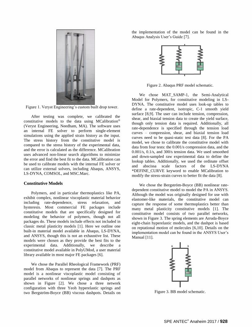
Figure 1. Veryst Engineering’s custom built drop tower.

After testing was complete, we calibrated the

constitutive models to the data using MCalibration®

(Veryst Engineering, Needham, MA). The software uses

an internal FE solver to perform single-element

simulations using the applied strain history as the input.

The stress history from the constitutive model is

compared to the stress history of the experimental data,

and the error is calculated as the difference. MCalibration

uses advanced non-linear search algorithms to minimize

the error and find the best fit to the data. MCalibration can

be used to calibrate models with the internal FE solver or

can utilize external solvers, including Abaqus, ANSYS,

LS-DYNA, COMSOL, and MSC.Marc.

Constitutive Models

Polymers, and in particular thermoplastics like PA,

exhibit complex, nonlinear viscoplastic material behavior

including rate-dependence, stress relaxation, and

hysteresis. Most commercial FE packages include

constitutive models that are specifically designed for

modeling the behavior of polymers, though not all

packages do. These models include effects not included in

classic metal plasticity models [1]. Here we outline one

built-in material model available in Abaqus, LS-DYNA,

and ANSYS, though this is not an exhaustive list. These

models were chosen as they provide the best fits to the

experimental data. Additionally, we describe a

constitutive model available in PolyUMod, a user material

library available in most major FE packages [6].

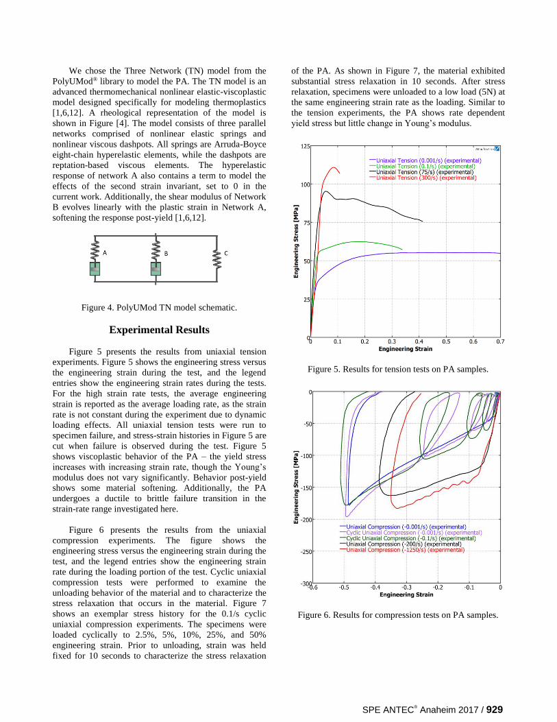
We chose the Parallel Rheological Framework (PRF)

model from Abaqus to represent the data [7]. The PRF

model is a nonlinear viscoplastic model consisting of

parallel networks of nonlinear springs and dashpots as

shown in Figure [2]. We chose a three network

configuration with three Yeoh hyperelastic springs and

two Bergström-Boyce (BB) viscous dashpots. Details on

the implementation of the model can be found in the

Abaqus Analysis User’s Guide [7].

Figure 2. Abaqus PRF model schematic.

We chose MAT_SAMP-1, the Semi-Analytical

Model for Polymers, for constitutive modeling in LS-

DYNA. The constitutive model uses look-up tables to

define a rate-dependent, isotropic, C-1 smooth yield

surface [8,9]. The user can include tension, compression,

shear, and biaxial tension data to create the yield surface,

though only tension data is required. Additionally, all

rate-dependence is specified through the tension load

curves – compression, shear, and biaxial tension load

curves need to be quasi-static test data [8]. For the PA

model, we chose to calibrate the constitutive model with

data from four tests: the 0.001/s compression data, and the

0.001/s, 0.1/s, and 300/s tension data. We used smoothed

and down-sampled raw experimental data to define the

lookup tables. Additionally, we used the ordinate offset

and abscissa scale factors of the LS-DYNA

*DEFINE_CURVE keyword to enable MCalibration to

modify the stress-strain curves to better fit the data [8].

We chose the Bergström-Boyce (BB) nonlinear rate-

dependent constitutive model to model the PA in ANSYS.

Although the model was originally designed for use with

elastomer-like materials, the constitutive model can

capture the response of some thermoplastics better than

many metal plasticity constitutive models [1]. The

constitutive model consists of two parallel networks,

shown in Figure 3. The spring elements are Arruda-Boyce

eight-chain hyperelastic models, and the dashpot is based

on reptational motion of molecules [6,10]. Details on the

implementation model can be found in the ANSYS User’s

Manual [11].

Figure 3. BB model schematic.


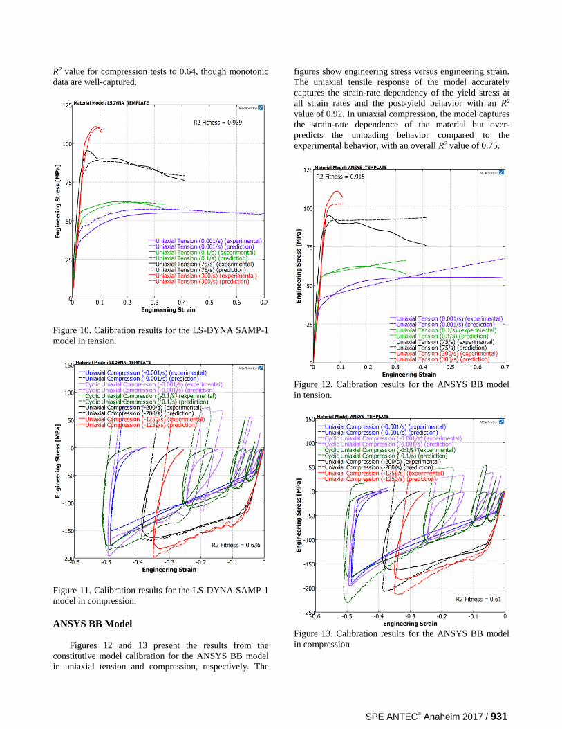
We chose the Three Network (TN) model from the

PolyUMod® library to model the PA. The TN model is an

advanced thermomechanical nonlinear elastic-viscoplastic

model designed specifically for modeling thermoplastics

[1,6,12]. A rheological representation of the model is

shown in Figure [4]. The model consists of three parallel

networks comprised of nonlinear elastic springs and

nonlinear viscous dashpots. All springs are Arruda-Boyce

eight-chain hyperelastic elements, while the dashpots are

reptation-based viscous elements. The hyperelastic

response of network A also contains a term to model the

effects of the second strain invariant, set to 0 in the

current work. Additionally, the shear modulus of Network

B evolves linearly with the plastic strain in Network A,

softening the response post-yield [1,6,12].

Figure 4. PolyUMod TN model schematic.

Experimental Results

Figure 5 presents the results from uniaxial tension

experiments. Figure 5 shows the engineering stress versus

the engineering strain during the test, and the legend

entries show the engineering strain rates during the tests.

For the high strain rate tests, the average engineering

strain is reported as the average loading rate, as the strain

rate is not constant during the experiment due to dynamic

loading effects. All uniaxial tension tests were run to

specimen failure, and stress-strain histories in Figure 5 are

cut when failure is observed during the test. Figure 5

shows viscoplastic behavior of the PA – the yield stress

increases with increasing strain rate, though the Young’s

modulus does not vary significantly. Behavior post-yield

shows some material softening. Additionally, the PA

undergoes a ductile to brittle failure transition in the

strain-rate range investigated here.

Figure 6 presents the results from the uniaxial

compression experiments. The figure shows the

engineering stress versus the engineering strain during the

test, and the legend entries show the engineering strain

rate during the loading portion of the test. Cyclic uniaxial

compression tests were performed to examine the

unloading behavior of the material and to characterize the

stress relaxation that occurs in the material. Figure 7

shows an exemplar stress history for the 0.1/s cyclic

uniaxial compression experiments. The specimens were

loaded cyclically to 2.5%, 5%, 10%, 25%, and 50%

engineering strain. Prior to unloading, strain was held

fixed for 10 seconds to characterize the stress relaxation

of the PA. As shown in Figure 7, the material exhibited

substantial stress relaxation in 10 seconds. After stress

relaxation, specimens were unloaded to a low load (5N) at

the same engineering strain rate as the loading. Similar to

the tension experiments, the PA shows rate dependent

yield stress but little change in Young’s modulus.

Figure 5. Results for tension tests on PA samples.

Figure 6. Results for compression tests on PA samples.


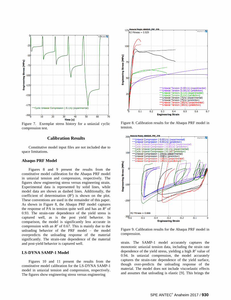
Figure 7. Exemplar stress history for a uniaxial cyclic

compression test.

Calibration Results

Constitutive model input files are not included due to

space limitations.

Abaqus PRF Model

Figures 8 and 9 present the results from the

constitutive model calibration for the Abaqus PRF model

in uniaxial tension and compression, respectively. The

figures show engineering stress versus engineering strain.

Experimental data is represented by solid lines, while

model data are shown as dashed lines. Additionally, the

coefficient of determination (R2) is shown on the plot.

These conventions are used in the remainder of this paper.

As shown in Figure 8, the Abaqus PRF model captures

the response of PA in tension quite well and has an R2 of

0.93. The strain-rate dependence of the yield stress is

captured well, as is the post yield behavior. In

comparison, the model is significantly less accurate in

compression with an R2 of 0.67. This is mainly due to the

unloading behavior of the PRF model – the model

overpredicts the unloading response of the material

significantly. The strain-rate dependence of the material

and post-yield behavior is captured well.

LS-DYNA SAMP-1 Model


constitutive model calibration for the LS-DYNA SAMP-1

model in uniaxial tension and compression, respectively.

The figures show engineering stress versus engineering

Figure 8. Calibration results for the Abaqus PRF model in

tension.

Figure 9. Calibration results for the Abaqus PRF model in

compression.

strain. The SAMP-1 model accurately captures the

monotonic uniaxial tension data, including the strain rate

dependence of the yield stress, yielding a high R2 value of

0.94. In uniaxial compression, the model accurately

captures the strain-rate dependence of the yield surface,

though over-predicts the unloading response of the

material. The model does not include viscoelastic effects

and assumes that unloading is elastic [9]. This brings the


R2 value for compression tests to 0.64, though monotonic

data are well-captured.

Figure 10. Calibration results for the LS-DYNA SAMP-1

model in tension.

Figure 11. Calibration results for the LS-DYNA SAMP-1

model in compression.

ANSYS BB Model


constitutive model calibration for the ANSYS BB model

in uniaxial tension and compression, respectively. The

figures show engineering stress versus engineering strain.

The uniaxial tensile response of the model accurately

captures the strain-rate dependency of the yield stress at

all strain rates and the post-yield behavior with an R2

value of 0.92. In uniaxial compression, the model captures

the strain-rate dependence of the material but over-

predicts the unloading behavior compared to the

experimental behavior, with an overall R2 value of 0.75.

Figure 12. Calibration results for the ANSYS BB model

in tension.

Figure 13. Calibration results for the ANSYS BB model

in compression


PolyUMod TN Model


constitutive model calibration for the PolyUMod TN

model in uniaxial tension and compression, respectively.

The figures show engineering stress versus engineering

strain. As shown in Figure 14, the TN model accurately

captures the response of PA in uniaxial tension with an R2

value of 0.94. Additionally, in uniaxial compression the

model captures the data well with an R2 value of 0.82.

This is mainly due to the TN model more accurately

predicting the cyclic uniaxial compression behavior,

particularly the stress relaxation and unloading to near-

zero load.

Figure 14. Calibration results for the PolyUMod TN

model in tension.

Discussion

Table 1 presents results comparing the coefficient of

determination for each calibrated model, showing the

results for all experiments, tension experiments only, and

compression experiments only. Table 1 shows that the TN

model more accurately predicts the experimental data

compared to the other models in both tension and

compression. The largest difference is due to the

improved performance in cyclic compression compared to

the other models, though tension results also show minor

improvements.

Although the accuracy of the constitutive models is

important to an FE problem, solution time must be

considered as well. More complex models generally

increase computing time for the problem and must be

considered. A simple FE model of an ASTM D638 Type

Figure 15. Calibration results for the PolyUMod TN

model in compression.

IV dogbone was created to run in each program to

compare the runtimes of the models. The models use

similar mesh geometries, loading conditions, boundary

conditions, and solver settings. Table 2 contains the

results for the model runtimes from these simulations. The

PolyUMod model was run in all solvers so that

comparisons can be made between models and between

FE programs. The TN model has a faster run time than the

Abaqus PRF model, but a slower run time than the LS-

DYNA SAMP-1 and the ANSYS BB models, though all

models have similar run times within the FE solver.

Table 1. Coefficients of determination for each model for

all load cases, tension, and compression.

An additional consideration for constitutive models is

in solver and element type support. The Abaqus PRF

model is supported for both implicit and explicit solvers

and all element types [7]. The LS-DYNA SAMP-1 model

is only available in the explicit solver [8]. Similarly, the

ANSYS BB model is only available in the implicit solver

[11]. Last, the implementation of the LS-DYNA SAMP-1

model is limited in that the material model is based on

lookup tables – the model does not include any

viscoelastic effects, and extrapolating outside the strain

Model

R2

All Tens. Comp.

Abaqus PRF 0.78 0.93 0.67

LS-DYNA SAMP-1 0.77 0.94 0.64

ANSYS BB 0.75 0.92 0.61

TN 0.87 0.94 0.82


rates tested does not yield a change in material response

[8-9].

Table 2. Coefficients of determination for each model for

all load cases, tension, and compression.

Model

Runtime (m:ss)

LS-

DYNA

Explicit

Abaqus/

Explicit

Abaqus/

Standard

ANSYS

Implicit

Abaqus

PRF N/A 1:25 1:42 N/A

LS-DYNA

SAMP-1 3:58 N/A N/A N/A

ANSYS BB N/A N/A N/A 0:17

TN 5:59 1:00 0:52 0:52

In contrast, the PolyUMod TN model is supported by

all three commercial FE packages studied here. This

includes both implicit and explicit FE solvers for Abaqus

and LS-DYNA, though only the implicit solver of

ANSYS is currently supported [6]. In addition to solver

support, the TN model is available for all element types.

The ability to use a particular model in multiple solvers

may be beneficial – the TN model is available for use in

all products, so switching FE packages is not an issue for

the end user. The BB model is available, in some form, in

all the FE packages studied here, though the specific

implementations are different and may require material

recalibration or verification [6-8,11].

Conclusions

We tested PA in uniaxial tension and compression

over six decades of engineering strain-rates and calibrated

material models to the experimental data using

MCalibration. All calibrated models captured major

features of the material response, though unloading

response of material models native to Abaqus, ANSYS,

and LS-DYNA was less than satisfactory. The PolyUMod

model best captured the unloading response. All models

had similar runtimes in the native FE solver, including the

TN model. Additionally, the PolyUMod constitutive

model had significant advantages in element type and

solver capabilities – it is available for explicit and implicit

solvers and all element types. Overall, the PolyUMod TN

model is best suited to model the response of the PA.

References

1. J. Bergström, Mechanics of Solid Polymers, (2015).

2. ASTM International. ASTM D638-14, Standard Test

Method for Tensile Properties of Plastics (2014).

3. S. Gurusideswar, R. Velmurugan, N Gupta, Polymer,

86, 197-207 (2016).

4. C. Roland, J. Twigg, Y. Vu, P. Mott, 2007. Polymer,

48, 574 – 578 (2007).

5. S. Teller, E. Schmitt, J. Bergström, ASME IMECE

Proceedings (2016).

6. PolyUMod® 4.4.3, Veryst Engineering, LLC (2016).

7. Abaqus® (2016), Abaqus Documentation, Dassault

Systèmes, Providence, RI.

8. LS-DYNA® Theory Manual, 2016 June 25, LSTC Inc.

9. S. Kolling, A. Haufe, M. Feucht, P. Du Bois, LS-

DYNA Anwenderforum (2005).

10. J. Bergström, M. Boyce, Journal of the Mechanics

and Physics of Solids, 46, 931-954 (1998).

11. ANSYS® Documentation, Release 16.1, ANSYS, Inc.

12. J. Bergström, J. Bischoff, International Journal of

Structural Changes in Solids, 2, 31-39 (2010).


high strain rate testing and modeling of polymers for...

Documents