high-speed oscilloscope fundamentals. digital... · 2019-10-17 · fundamentals. 2 •time domain...

是德科技資深應用工程師

邱柏勝

High-Speed Oscilloscope Fundamentals

2

• Time Domain vs. Frequency Domain

• Sampling Rate and Modes

• Bandwidth and Aliasing

• Oscilloscope Architectures

• Waveform Update Rate

• Memory Depth and Methods

• Triggering: Basics and Advanced

• Waveform Visualization Tools

• Probing Architecture, Tips and Tricks

A G E N D A S L I D E

3

Am

plit

ud

e

Time Domain Measurements

Frequency Domain Measurements

4

Frequency Domain Applications

Spectrum Analyzer

Network Analyzer

FFT Analyzer

Signal Analyzer

FFT function on an Oscilloscope

Time Domain Applications

Oscilloscope

Signal Analyzer

Network Analyzer

M E A S U R E M E N T D E V I C E S

5

• A mathematical conversion between time and

frequency domain can always be performed

• Fast Fourier Transform (FFT) – less calculations

• FFT - easily processed by a computer

• Alternative ways of representing the same signal

• Some behavior is seen easier in one domain

H O W T O C O N V E R T B E T W E E N T H E T W O – O R H AV E B O T H !

6











7

• The speed at which the oscilloscope samples the voltage of the input signal. Measured in samples

per second (Sa/s)

• The signal you see on screen is actually a “connect the dots” image of up to billions of samples to

create a continuous shape over time.

• The minimum sample rate varies from ~2.5x to 5x the oscilloscope bandwidth. E.g. 1 GHz needs 5

GSa/s

H O W O F T E N T H E O S C I L L O S C O P E M E A S U R E S V O LTA G E – S A M P L E R AT E

8

• All samples are taken on a single

trigger event

• Pre-trigger acquisition is possible

(data before trigger)

• Bandwidth depends on sampling

frequency

• Sampling frequency is also called

the digitizing rate

• Resolution of points on screen is

1/sample rate

R E A L - T I M E S A M P L I N G

11

1

1 1 11

1

1 1

Sample Clock

9

• Sample clock is asynchronous to input

• Pre-trigger acquisition is possible (data

before trigger)

• Requires a repetitive waveform.

Waveform "BUILDS-UP" with repetitive

input.

• Bandwidth / sample density is not limited

by sample rate

• Repetitive bandwidth is limited only by

analog bandwidth

• Not in common use today

E Q U I VA L E N T T I M E S A M P L I N G – “ R A N D O M R E P E T I T I V E ”

DIGITIZEDWAVEFORM

ASYNCSAMPLECLOCK

TRIGGERLEVEL

TriggerT=0

ACQ #1

ACQ #2

ACQ #3

+/- x psec

10

• One sample is taken on each

trigger - the acquisition is slower

• Requires repetitive signal

• NO pre-trigger view (no data

before the trigger point)

• Even increments of delay after

each trigger

• Delay interval very small giving

better timing resolution (higher BW)

• Provides very accurate waveform

reconstruction - uses slower, higher

resolution A/D Converters

S E Q U E N T I A L S A M P L I N G

10

13

9 11 1315

17

19 21

4 7

8

5

12 14 16

18 202 6

Trigger

11

H I G H R E S O L U T I O N M O D E – R E A L - T I M E S C O P E S

1.5MHz clock with High Resolution sampling1.5MHz clock with Real-Time sampling

• Waveform is sampled at maximum rate

• Samples from the same trigger are averaged

• Reduces noise at the expense of bandwidth

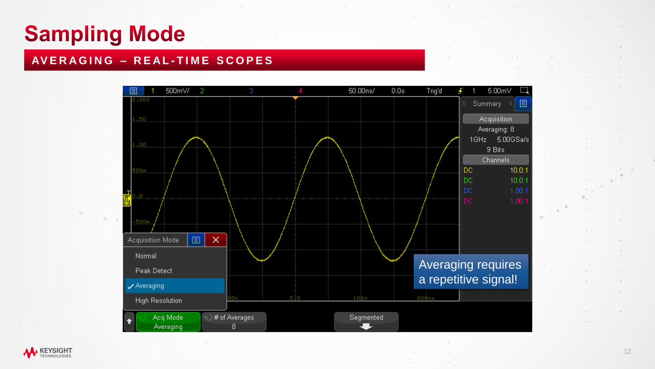
12

AV E R A G I N G – R E A L - T I M E S C O P E S

Averaging requires

a repetitive signal!

13











14

• Defines the fastest signal the oscilloscope can capture. Any signals faster than the bandwidth of

the scope will not be accurate, or may not even be shown at all.

• In datasheets, defined along with “rise time”.

T H E D E F I N I N G C H A R A C T E R I S T I C O F A N O S C I L L O S C O P E

15

A L S O C A L L E D T H E “ 3 D B D O W N P O I N T ”

Frequency

-3dB

Att

en

ua

tio

n

0dB

BW

Maximally-flat Response

Gaussian Response

Scope swept response measurement

16

H O W M U C H B A N D W I D T H D O Y O U N E E D ?

Required

Accuracy

Gaussian

Response

Maximally-flat

Response

20% BW = 1.0 x fknee BW = 1.0 x fknee



Step #2: Determine highest signal frequency content (fknee).fknee = 0.5/RT (10% - 90%)fknee = 0.4/RT (20% - 80%)

Step #3: Determine degree of required measurement accuracy.Scope BW Calculation

Step #4: Calculate required bandwidth.

Step #1: Determine fastest rise/fall times of device-under-test.

Source: Dr. Howard W. Johnson, “High-speed Digital Design – A Handbook of Black Magic”

17

H O W M U C H B A N D W I D T H D O I R E A L LY N E E D ?

Determine the minimum bandwidth of an oscilloscope

(assume Gaussian frequency response) to measure

signals that have rise times as fast as 500 ps (10-90%):

fknee (10-90%)= (0.5/RT) = (0.5/0.5 ns) = 1 GHz

20% Accuracy: BW = 1.0 x fknee = 1.0 x 1 GHz = 1.0 GHz

3% Accuracy: BW = 1.9 x fknee = 1.9 x 1 GHz = 1.9 GHz

18

W H AT H A P P E N S I F M Y O S C I L L O S C O P E I S T O O S L O W ?

Response using a 100-MHz BW scope

What does a 100-MHz clock signal really look like?

Response using a 500-MHz BW scope

19

• Nyquist’s sampling theorem states that for a limited

bandwidth (band-limited) signal with maximum frequency

fmax, the equally spaced sampling frequency fs must be

greater than twice of the maximum frequency fmax, i.e.,

fs > 2·fmax

• in order to have the signal be uniquely reconstructed without

aliasing.

• The frequency 2·fmax is called the Nyquist sampling

frequency (fS). Half of this value, fmax, is sometimes called

the Nyquist frequency (fN).

N Y Q U I S T ’ S T H E O R E M : R E M E M B E R I N G T H E C O L L E G E D AY S

Dr. Harry Nyquist, 1889-1976,

articulated his sampling

theorem in 1928

Sample points

Original

Aliased signal

20

N O T F E A S I B L E I N T H E R E A L W O R L D

fSfN

-3dB

Frequency

0dBA

tte

nu

ati

on

21

S A M P L E R AT E I S T W I C E B A N D W I D T H

Frequency

-3dB

Att

en

ua

tio

n0dB

fN fS

Aliased Frequency Components

22

S A M P L E R AT E I S F O U R T I M E S B A N D W I D T H

Frequency

-3dB

Att

en

ua

tio

n0dB

fN fSfS/4


23

S A M P L E R AT E I S 2 . 5 X B A N D W I D T H

Frequency

-3dB

Att

en

ua

tio

n0dB

fN fSfS/2.5


24

E V E R Y S I G N A L C O N S I S T S O F A F U N D A M E N TA L A N D I T S H A R M O N I C S

Fundamental

2nd Harmonic

4th Harmonic

5th Harmonic

3rd Harmonic

FREQUENCY

AM

PL

ITU

DE

FREQUENCY

DOMAIN

TIME DOMAIN

TIMEA

MP

LIT

UD

E

1

2

3

4

5

25

D I S T O R T I O N D U E T O A L I A S I N G A N D B A N D W I D T H L I M I T I N G

ACTUAL PULSE DISPLAYED PULSE

26

I N P U T T E S T S I G N A L : 1 N S W I D E P U L S E W I T H 5 0 0 P S R I S E T I M E

2.5 GSa/s

RT = 580 ps ± 60 ps

RTσ = 24 ps

PW = 964 ps ± 50 ps

PWσ = 20 ps

5 GSa/s

RT = 550 ps ± 30 ps

RTσ = 8.7 ps

PW = 985 ps ± 30 ps

PWσ = 9.5 ps

SR = BW x 2.5

SR = BW x 5

27











28

B A S I C O S C I L L O S C O P E B L O C K D I A G R A M

29

I N F I N I I V I S I O N X - S E R I E S : S C O P E O N A C H I P F O R M A X P E R F O R M A N C E

30

H O W T O A C Q U I R E H I G H E R B A N D W I D T H S I G N A L S T H A N Y O U R S C O P E ’ S S A M P L E R

Tektronix Asynchronous

Time Interleave (ATI)

Teledyne LeCroy

Digital Bandwidth Interleave (DBI)

• Time-Interleaved Sampling (TIS) used in traditional oscilloscopes

was unable to keep pace with industry bandwidth demands

• The fastest TIS technologies maxed out at < 40 GHz

• Frequency based interleaving bridged the bandwidth gap

• Splits an incoming signal into a low and high frequency path

• Enabled multiple slower samplers to acquire higher BW inputs

• Splitting, amplifying and recombining frequency bands is complicated

and inherently degrades signal integrity

• Downside is creating superfluous noise, spurs and aliasing

31

Front End Multi-Chip Module

T O M O R R O W S S C O P E H A R D W A R E A R C H I T E C T U R E - T O D AY

Timebase

10 Bit ADC

Edge Trigger

AdvancedTrigger

Memory Controller

HMC

Link to CPU

Sampler(30 GHz)

ElectromechanicalAttenuator

Buffer AmpSampler(110 GHz)

Pre-amp(110 GHz)

InP InP

Some Highlights

• No Frequency based Interleaving – provides a full bandwidth InP enabled sampling system

• Much higher frequency and more efficient data flow w/ less noise

• Adapts the latest technologies, including HMC and faraday cage Front End Multi-chip modules

32











33

H O W O F T E N C A N T H E O S C I L L O S C O P E S H O W M E WAV E F O R M S ?

Improves scope usability

Improves scope display quality

Improves scope probability of

capturing infrequent events

34

V I S U A L I Z I N G T H E D I F F E R E N C E

Long Dead Time = Decreases the chance of capturing rare events

Scope with a slower update rate

Scope with a faster update rate

Short Dead Time = Increases the chance of capturing rare events

35

• A slower update rate means you may miss important, fast moving, and rare events on a signal that

are very important to see.

• Each acquisition is like a roll of the dice – the more often you roll the dice, the better chance you

can get all possible outcomes!

W H AT H A P P E N S I F M Y U P D AT E R AT E I S T O O S L O W ?

No Glitches Captured Multiple Glitches

Captured

36











37

• Measured in samples or points. Modern scopes have millions or billions of samples in memory.

• More memory means more time can be shown on screen using maximum sample rate. But, more

memory adds cost, slows down the responsiveness of the scope, and adds complexity.

• Keysight InfiniiVision X-Series are the only scopes in the market that automatically adjust memory

depth to maximize performance. Others will give the user a setting to adjust manually.

H O W M A N Y S A M P L E S C A N T H E O S C I L L O S C O P E TA K E AT O N C E ?

𝑀𝑒𝑚𝑜𝑟𝑦 𝐷𝑒𝑝𝑡ℎ 𝑆𝑎 = 𝑆𝑎𝑚𝑝𝑙𝑒 𝑅𝑎𝑡𝑒𝑆𝑎

𝑠∗ 𝑇𝑖𝑚𝑒 (𝑠)

38

• Every sample must be stored in memory

• Deeper memory stores more samples

• Longer periods of time means more samples to store in order to maintain sample rate

P U R P O S E O F M E M O R Y I N D I G I T I Z I N G S C O P E S

39

Maintain High Sample Rate While Capturing Longer Periods of Time

Ability to zoom-in and see all the details

Higher Sample Rate =• Capture higher BW signals (remember Nyquist?)

Especially important in• Mixed analog and digital applications

• Serial communication applications

T H E P U R P O S E O F D E E P M E M O R Y

Group/Presentation Title

Keysight Restricted

Month ##, 200X

40

Determine required sample rate

• Usually based on fastest clock rate or rise time

Determine longest time-span to acquire

• Usually based on slowest analog signal or digital packets

H O W M U C H M E M O R Y D O I N E E D ?

Example:

Required Sample Rate = 2 GSa/s

Sample Interval = 1/SR = 500 ps/Sa

Longest Time Span = 2 ms (200 µs/div)

Required Memory Depth

= 2 ms / 500 ps/Sa

= 4 MSa

𝑀𝑒𝑚𝑜𝑟𝑦 𝐷𝑒𝑝𝑡ℎ 𝑆𝑎 = 𝑆𝑎𝑚𝑝𝑙𝑒 𝑅𝑎𝑡𝑒𝑆𝑎

𝑠∗ 𝑇𝑖𝑚𝑒 (𝑠)

41

• Slower Waveform Update Rate

• Slower User-Input Response Time

• Increased Dead-Time Between Acquisitions

• Missed Glitches and Anomalies during Dead-Time

P O S S I B L E N E G AT I V E I M P L I C AT I O N S O F D E E P M E M O R Y


Keysight Restricted

Month ##, 200X

42

Custom ASIC hardware built into acquisition system

• Keysight’s MegaZoom Technology

MegaZoom is a Memory Management Tool

• Ping-Pong acquisition memory

• Preprocessing of data in hardware

• No special modes – always on and always fast

Result is a fast waveform update rate with minimal

dead-time between acquisitions and no processing

bottlenecks.

S O LV I N G T H E D E A D - T I M E P R O B L E M I N D E B U G O S C I L L O S C O P E S


Keysight Restricted

Month ##, 200X

43











44

R I N G A C Q U I S I T I O N M E M O R Y

The oscilloscope is constantly acquiring data if no trigger event occurs. The acquisition

memory is overwritten with new data.

When a trigger event occurs the memory content (waveform data) is transferred to the

Display Memory and a new acquisition starts.

Trigger

Ring Model Linear Model

Beginning EndTrigger

Post-store

23 289

Pre-store

23

2425

262728

9

10

17

14

13

12

11

18

22

1615

21

20

19

45

B A S I C R I S I N G E D G E T R I G G E R ( D E FA U LT )

Trigger Point

Trigger Point

Untriggered / Auto-Trigger(unsynchronized picture taking)

Rising edge @ 0.0 V

Rising edge @ +785 mV

Trigger level set above waveform

Positive TimeNegative Time

46

A U T O V S . N O R M A L : W H AT ’ S W I T H T H E S C O P E S PA G H E T T I ?

Auto trigger: “I don’t see a

trigger: I’ll trigger on my own”

Normal trigger: “I don’t see a

trigger, I’ll do nothing at all”

47

A D VA N C E D O S C I L L O S C O P E T R I G G E R I N G

Example: Triggering on an I2C serial bus

Much of your oscilloscope

use will only require standard

“edge” triggering.

Sometimes your signal is

more complex, like this serial

bus.

Triggering on more complex

signals requires advanced

triggering options.

48

H O W T O D E A L W I T H N O I S Y S I G N A L S

Rising edge trigger – Scope

triggers on high frequency

noise during a falling edge of

sine wave

Rising edge trigger, HF Reject –

Scope correctly triggers on high

frequency noise

49

H O W T O D E A L W I T H N O I S Y S I G N A L S

Standard Oscilloscope TriggeringEdge

Pattern

Video

Advanced Parametric TriggeringPulse-width

Nth Edge Burst

Setup & Hold Time

Runt

Edge Speed

Serial Bus TriggeringI2C, SPI, RS232/UART, I2S, CAN, LIN, FlexRay, SENT, MIL-STD 1553

50











51

Color gradation and histograms provide graphical

representation of signal and measurement distributions.• Also see the distributions of some measurement results.

• An independent database for color gradation gives flexibility.

• Because color gradation/histograms operate like a function, they can be applied to analog waveforms, reference waveforms, and math functions, like FFT.

• Measurement histograms display a graphical distribution of the measurement results.

V I S U A L I Z E T H E S I G N A L D I S T R I B U T I O N :

C O L O R G R A D E + H I S T O G R A M

Color grade & histogram

Measurement histogram

52











53

R E S I S T O R D I V I D E R P R O B E S – B L O C K D I A G R A M

Passive 10:1 Probe Model

• Capacitors act as open circuits at low frequency.

• Inductors act as short circuits at low frequency.

• Simplifies to a 9 MΩ resistor in series with the scope’s 1 MΩ input

termination.

54

R E S I S T O R D I V I D E R P R O B E S – B L O C K D I A G R A M

Where Cparallel = Ccomp + Ccable + Cscope

• At high frequencies, we get an impedance divider, because

capacitors will begin to express non-real resistances on our circuit.

• Ccomp is adjusted by the user to create a 10:1 divider of capacitive

elements using the following formula:

55

R E S I S T O R D I V I D E R P R O B E S – L O A D I N G C H A R A C T E R I S T I C S

probe loading

Lower

Higher

N2873A 500 MHz Passive Probe10 MΩ, 9.5 pF

1.E+00

1.E+01

1.E+02

1.E+03

1.E+04

1.E+05

1.E+06

1.E+07

1.E+08

1.E+01 1.E+02 1.E+03 1.E+04 1.E+05 1.E+06 1.E+07 1.E+08 1.E+09 2.E+09

~150 Ω

70 MHz

Imp

ed

ance

(oh

m)

Frequency (Hz)

10 kHz

56

A C T I V E P R O B E L O A D I N G I S S U P E R I O R T O PA S S I V E

10 kHz probe loading

Lower

Higher

N2873A 500 MHz Passive Probe10 MΩ, 9.5 pF

1.E+00

1.E+01

1.E+02

1.E+03

1.E+04

1.E+05

1.E+06

1.E+07

1.E+08

1.E+01 1.E+02 1.E+03 1.E+04 1.E+05 1.E+06 1.E+07 1.E+08 1.E+09 2.E+09

~2.5 kΩ

~150 Ω

70 MHz

Imp

ed

ance

(oh

m)

Frequency (Hz)

N2796A 2 GHzActive Probe1 MΩ, 1 pF

57

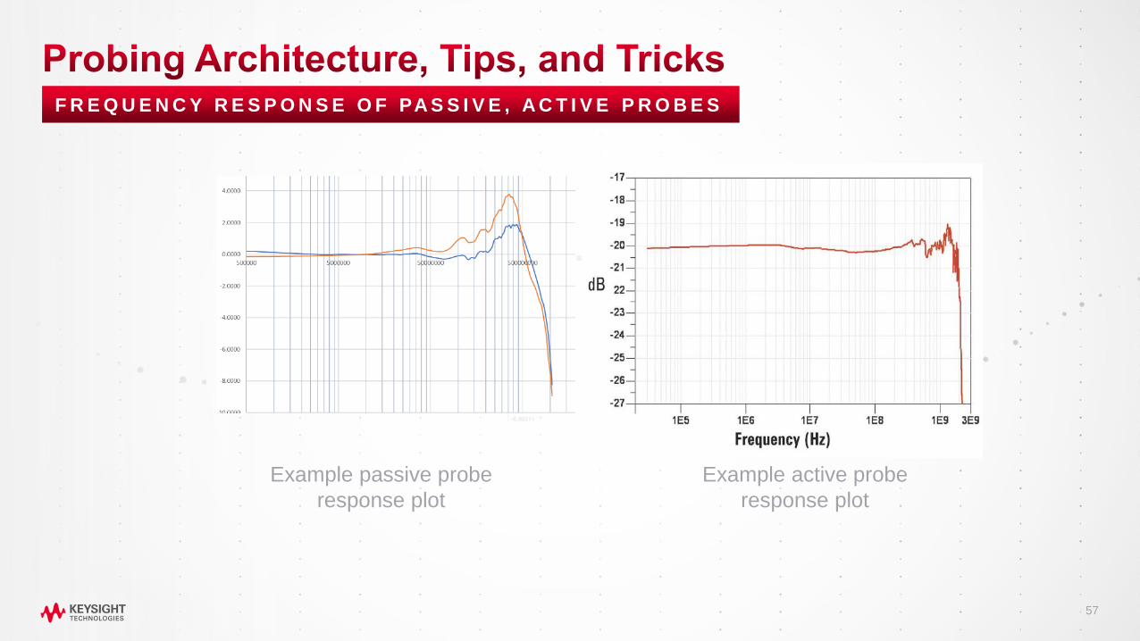
F R E Q U E N C Y R E S P O N S E O F PA S S I V E , A C T I V E P R O B E S

Example active probe

response plot

Example passive probe

response plot

59

• Keysight Digital Learning Center www.keysight.com/find/klcdigital

• Webcast Recordings and Technical seminar videos , Application Notes • USB Type-C , PAM-4 , PCI-Express, DDR Memory

• Signal Integrity , Power Integrity

• Measurement Fundamentals for AWG, BERT, Scope etc.

• Keysight RF and Digital Monthly Webcast Series

• Live and On Demand Viewing : www.keysight.com/find/webcastseries (U.S. Version)

• Register for Future Webcasts : https://kee.smarket.net.cn/2019/index.html (中文平台)

• Keysight 大型活动

• 感恩月历届技术干货汇总：2017年感恩月示波器文章，示波器技术文章回顾

• Keysight World 2019 技术演讲回看

• Oscilloscope Topics at Youtube :

• Sampling: https://www.youtube.com/watch?v=yBC97UUljKo

• Bandwidth: https://www.youtube.com/watch?v=VBJWkceO1OA

• Update Rate: https://www.youtube.com/watch?v=CPDIrKSDrZk

• Memory Depth: https://www.youtube.com/watch?v=GAM_CpxVYq8

• Eye Diagrams: https://www.youtube.com/watch?v=mnugUjaMN70

http://www.keysight.com/find/klcdigital

https://www.keysight.com/main/editorial.jspx?cc=US&lc=eng&ckey=2917052&id=2917052

https://www.keysight.com/main/editorial.jspx?cc=CN&lc=chi&ckey=2960680&id=2960680

http://www.keysight.com/find/

http://www.keysight.com/find/webcastseries

https://kee.smarket.net.cn/2019/index.html

https://mp.weixin.qq.com/s/6dmzwhOi-v7OJA72G7WPrw

https://keysighttube.smarket.net.cn/app/views/searchList.html?searchType=topicType&searchValue=Keysight%20World%202019

https://www.youtube.com/watch?v=yBC97UUljKo

https://www.youtube.com/watch?v=VBJWkceO1OA

https://www.youtube.com/watch?v=CPDIrKSDrZk

https://www.youtube.com/watch?v=GAM_CpxVYq8

https://www.youtube.com/watch?v=mnugUjaMN70

Speaker Title / Company Name

Speaker Name

示波器基础典型应用分享

62

示波器典型应用分享

Keysight Territory Turbo Program

• 是德科技抖示波器家族简介

63

Keysight示波器家族

Infiniium 系列• 实时带宽：超过100 GHz

• 存储：深达2G每通道• 操作系统：Windows Z 系列 20-63GHz

U160020MHz

~40MHz

3000 X系列100 MHz

~1GHz

4000 X系列200 MHz~1.5GHz

InfiniiVision 系列• 带宽: 50 MHz ～ 6 GHz

• 独特技术：直观显示信号• 操作系统：嵌入式

S 系列 500MHz-8GHz

6000 X系列1GHz

~6GHz

P924XAUSB示波器

200MHz~1GHz

2000 X系列70 MHz

~200MHz

1000 X系列50 MHz

~100MHz

V 系列 8-33GHz

多样化

• 手持式、USB无脸式、PXIe模块

• 便携式、台式

• 嵌入式操作系统、Windows操作系统

• 8-bit ADC , 10-bit ADC

U924XAPXIe示波器

200MHz~1GHz

UXR 系列 13-110GHz 10-bit ADC

high-speed oscilloscope fundamentals. digital... · 2019-10-17 · fundamentals. 2 •time domain...

Documents