high performance parallel computing of flows in complex

Computational Science & Discovery

High performance parallel computing of flows incomplex geometries: I. MethodsTo cite this article: N Gourdain et al 2009 Comput. Sci. Discov. 2 015003

View the article online for updates and enhancements.

You may also likeResolution modeling in projection spaceusing a factorized multi-block detectorresponse function for PET imagereconstructionHancong Xu, Mirjam Lenz, Liliana Caldeiraet al.

-

CFD code comparison for 2D airfoil flowsNiels N. Sørensen, B. Méndez, A. Muñozet al.

-

Lattice Boltzmann methods for movingboundary flowsTakaji Inamuro

-

Recent citationsNumerical Prediction of the Aerodynamicsand Acoustics of a Tip Leakage FlowUsing Large-Eddy SimulationDavid Lamidel et al

-

2D radial-azimuthal particle-in-cellbenchmark for E × B dischargesW Villafana et al

-

A mesh adaptation strategy for complexwall-modeled turbomachinery LESNicolas Odier et al

-

This content was downloaded from IP address 220.87.216.167 on 31/12/2021 at 10:55

https://doi.org/10.1088/1749-4699/2/1/015003

https://iopscience.iop.org/article/10.1088/1361-6560/ab266b




https://iopscience.iop.org/article/10.1088/1742-6596/753/8/082019



https://doi.org/10.3390/ijtpp6030027



http://iopscience.iop.org/0963-0252/30/7/075002







https://doi.org/10.1016/j.compfluid.2020.104766

https://doi.org/10.1016/j.compfluid.2020.104766

High performance parallel computing of flows incomplex geometries: I. Methods

N Gourdain1, L Gicquel1, M Montagnac1, O Vermorel1, M Gazaix2,G Staffelbach1, M Garcia1, J-F Boussuge1 and T Poinsot3

1 Computational Fluid Dynamics Team, CERFACS, Toulouse, 31057, France2 Computational Fluid Dynamics and Aero-acoustics Department, ONERA, Châtillon,92320, France3 Institut de Mécanique des Fluides de Toulouse, Toulouse, 31400, FranceE-mail: [email protected]

Received 16 June 2009, in final form 29 September 2009Published 12 November 2009Computational Science & Discovery 2 (2009) 015003 (26pp)doi:10.1088/1749-4699/2/1/015003

Abstract. Efficient numerical tools coupled with high-performance computers, havebecome a key element of the design process in the fields of energy supply and transportation.However flow phenomena that occur in complex systems such as gas turbines and aircrafts arestill not understood mainly because of the models that are needed. In fact, most computationalfluid dynamics (CFD) predictions as found today in industry focus on a reduced or simplifiedversion of the real system (such as a periodic sector) and are usually solved with a steady-state assumption. This paper shows how to overcome such barriers and how such a newchallenge can be addressed by developing flow solvers running on high-end computingplatforms, using thousands of computing cores. Parallel strategies used by modern flowsolvers are discussed with particular emphases on mesh-partitioning, load balancing andcommunication. Two examples are used to illustrate these concepts: a multi-block structuredcode and an unstructured code. Parallel computing strategies used with both flow solvers aredetailed and compared. This comparison indicates that mesh-partitioning and load balancingare more straightforward with unstructured grids than with multi-block structured meshes.However, the mesh-partitioning stage can be challenging for unstructured grids, mainly due tomemory limitations of the newly developed massively parallel architectures. Finally, detailedinvestigations show that the impact of mesh-partitioning on the numerical CFD solutions,due to rounding errors and block splitting, may be of importance and should be accuratelyaddressed before qualifying massively parallel CFD tools for a routine industrial use.

Computational Science & Discovery 2 (2009) 015003 www.iop.org/journals/csd2009 IOP Publishing Ltd 1749-4699/09/015003+26$30.00

mailto:[email protected]

http://dx.doi.org/10.1088/1749-4699/2/1/015003

http://www.iop.org/journals/csd

Computational Science & Discovery 2 (2009) 015003 N Gourdain et al

Contents

1. Introduction 3

2. Presentation of the flow solvers 3

3. Parallel efficiency 53.1. Definition of the task scalability . . . . . . . . . . . . . . . . . . . . . . . . . . . . . . . . . 53.2. Flow solver scalability . . . . . . . . . . . . . . . . . . . . . . . . . . . . . . . . . . . . . . 6

4. Mesh partitioning strategies 74.1. General organization . . . . . . . . . . . . . . . . . . . . . . . . . . . . . . . . . . . . . . . 84.2. Structured multi-block meshes . . . . . . . . . . . . . . . . . . . . . . . . . . . . . . . . . . 94.3. Unstructured meshes . . . . . . . . . . . . . . . . . . . . . . . . . . . . . . . . . . . . . . . 11

5. Communication and scheduling 165.1. Presentation of message passing protocols . . . . . . . . . . . . . . . . . . . . . . . . . . . . 165.2. Blocking and non-blocking message passing interface communications . . . . . . . . . . . . . 165.3. Point-to-point and collective message passing interface communications . . . . . . . . . . . . 17

6. Memory management 206.1. RAM requirements . . . . . . . . . . . . . . . . . . . . . . . . . . . . . . . . . . . . . . . . 206.2. Memory bandwidth . . . . . . . . . . . . . . . . . . . . . . . . . . . . . . . . . . . . . . . . 21

7. Impact on numerical solutions 217.1. Mesh-partitioning and implicit algorithms . . . . . . . . . . . . . . . . . . . . . . . . . . . . 227.2. Rounding errors and large eddy simulation . . . . . . . . . . . . . . . . . . . . . . . . . . . . 22

8. Conclusion and further works 23

Acknowledgment 24

References 25

Nomenclature

ALE arbitrary Lagrangian EulerianAPI application program interfaceCFD computational fluid dynamicsDES detached eddy simulationsDTS dual time steppingFLOPS FLoating-point Operation Per SecondHPC high-performance computingI/O input/output (data)IPM integrated parallel macrosLES large eddy simulationMPI message passing interfaceMIMD multiple instructions, multiple dataMPMD multiple programs multiple dataPU processing unit (i.e. a computing core4)RANS Reynolds-averaged Navier–StokesRCB recursive coordinate bisectionREB recursive edge bisectionRGB recursive graph bisectionRIB recursive inertial bisectionSPMD single program multiple data

4 In this paper, it is assumed that one computing core is dedicated to only one process.

2


1. Introduction

Computational fluid dynamics (CFD) is the simulation, by computational methods, of the governing equationsthat describe the fluid flow behaviour (usually derived from the Navier–Stokes equations). It has grown froma purely scientific discipline to become an essential industrial tool for fluid dynamics problems. A widevariety of applications can be found in the literature, ranging from nuclear to aeronautic applications. IndeedCFD flow solvers are considered to be standard numerical tools in industry for design and development,especially for aeronautic and propulsion domains. This approach is attractive since it reproduces physical flowphenomena more rapidly and at a lower cost than experimental methods. However, industrial configurationsremain complex and CFD codes usually require high-end computing platforms to obtain flow solutions in areasonable amount of time. Within the real of computing architectures, high performance computing (HPC)has no strict definition but it usually refers to (massively) parallel processing for running quickly applicationprograms. The term applies especially to systems that work above 1012 FLoating-point Operation Per Second(FLOPS) but it is also used as a synonym for supercomputing. Two kinds of architecture are generally set apart.The first one is the vector architecture that has high-memory bandwidth and vector processing capabilities.The second architecture relies on superscalar cache-based computing cores interconnected to form systems ofsymmetric multi-processing nodes and has rapidly developed over the past decade due to the cost effectivenessof its basic components. This tendency is best illustrated by the list of the Peak Performance Gordon BellPrize, delivered each year at the supercomputing conference and which rewarded applications running onmassively parallel scalar platforms for the last successive three years after a period dominated by vectorsupercomputers (www.top500.org). However, some difficulties are still observed with cached-based processorssince the common computing efficiency is less than 20% for most CFD applications (Keyes et al 1997). Oneof the reasons is that flow solvers process a large amount of data, meaning a lot of communication is requiredbetween the different cache levels. Indeed such parallel platforms impose to run tasks on a large number ofcomputing cores to be attractive and provide new possibilities for CFD by reducing computational time andgiving access to large amounts of memory.

Parallel platforms integrate many processors that are themselves composed of one or more computingcores (a processing unit (PU) corresponds to the task performed by one computing core). Programming forparallel computing where simultaneous computing resources are used to solve a problem can become verychallenging and performance is related to a great quantity of parameters. With a relatively small number ofPU (<128), calculations efficiency relies essentially on communications as they are the primary parametersthat counterbalance the architecture peak power. When thousands of PUs are used, load balancing betweencores and communications dominate and both aspects clearly become the limiting factors of computationalefficiency. This paper focuses on the work done in flow solvers to efficiently run on these powerfulsupercomputers. Objectives are to show techniques and methods that can be used to develop parallel computingaspects in CFD solvers and to give an overview of the authors’ daily experience when dealing with suchcomputing platforms. There is no consensus today in the CFD community on the type of mesh or datastructure to use on parallel computers. Typically, flow solvers are usually efficient to solve the flow inonly one specific field of applications such as combustion, aerodynamics, etc. Two different flow solversare considered here to illustrate the different tasks that have to be considered to obtain a good efficiencyon HPC platforms, with a special interest for (massively) parallel computing: a multi-block structured flowsolver dedicated to aerodynamics problems (elsA) and an unstructured flow solver designed for reactive flows(AVBP). Mesh partitioning and load balancing strategies considered by both solvers are discussed. Impactof HPC oriented programming, code architecture and the physical solutions they provide are also described.

2. Presentation of the flow solvers

Modern flow solvers have to efficiently run on a large range of supercomputers, from single core tomassively parallel platforms. The most common systems used for HPC applications are the multipleinstruction multiple data (MIMD) based platforms (Flynn 1972). This category can be further divided in two

3

http://www.top500.org


sub-categories:

• Single program, multiple data (SPMD). Multiple autonomous PUs simultaneously executing the sameprogram (but at independent points) on different data. The flow solver elsA is an example of a SPMDprogram;

• Multiple program, multiple data (MPMD). Multiple autonomous PUs simultaneously operating at leasttwo independent programs. Typically such systems pick one PU to be the host (the ‘master’), which runsone program that farms out data to all the other PUs (the ‘slaves’) which all run a second program. Thesoftware AVBP uses this method, referred as the ‘master-slave’ strategy.

The elsA software is a reliable design tool in the process chains of aeronautical industry and is intensively usedby several major companies (Cambier and Gazaix 2002, Cambier and Veuillot 2008). This multi-applicationCFD simulation platform deals with internal and external aerodynamics from low subsonic to hypersonic flowregime. The compressible 3D Navier–Stokes equations for arbitrary moving bodies are considered in severalformulations according to the use of absolute or relative velocities. A large variety of turbulence modelsfrom eddy viscosity to full differential Reynolds stress models is implemented for the Reynolds-averagedNavier–Stokes (RANS) equations (Davidson 2003), including criteria to capture laminar-turbulent transitionphenomena for academic and industrial geometries (Cliquet et al 2007). In order to deal with flows exhibitingstrong unsteadiness or large separated regions, high-fidelity methods such as detached eddy simulation (DES)(Deck 2005, Spalart et al 1997) and large eddy simulation (LES) (Smagorinsky 1963) are also available.For computational efficiency reasons, connectivity and data exchange between adjacent blocks are set bymeans of ghost cells. High-flexibility techniques of multi-block structured meshes have been developed to dealwith industrial configurations. These advanced techniques include totally non-coincident interfaces (Fillolaet al 2004) and the Chimera technique for overlapping meshes (Meakin 1995). The flow equations are solvedby a cell centred finite-volume method. Space discretization schemes include upwind schemes (Roe 1981;AUSM, Liou 1996) or centred schemes, stabilized by scalar or matrix artificial dissipation. The semi-discreteequations are integrated, either with multistage Runge–Kutta schemes or with a backward Euler integrationthat uses implicit schemes solved by robust lower-upper (LU) relaxation methods (Yoon and Jameson 1987).For time accurate computations, the implicit dual time stepping (DTS) method is available (Jameson 1991).Several programming languages are used to develop the elsA software: C++ as main language for implementingthe object-oriented design (backbone of the code), Fortran for CPU efficiency in calculation loops and Pythonfor user interface. The code has already been ported on a very large variety of platforms, including vector andmassively scalar supercomputers. Vector capabilities are still supported, but focus today is clearly on scalarparallel platforms with an increasing number of computing cores. To run in parallel, elsA uses a simple coarse-grained SPMD approach, where each block is allocated to a PU (note that in some circumstances several blockscan be allocated to the same PU). To achieve a good scalability, a load-balancing tool with block-splittingcapability is included in the software.

The AVBP project was historically motivated by the idea of building a modern software tool forCFD with high flexibility, efficiency and modularity. Recent information about this flow solver can befound in Garcia (2009). This flow solver is used in the frame of cooperative works with a wide range ofindustrial companies. AVBP is an unstructured flow solver capable of handling hybrid grids of many celltypes (tetra/hexahedra, prisms, etc). The use of these grids is motivated by the efficiency of unstructuredgrid generation, the accuracy of the computational results (using regular structured elements) and the easeof mesh adaptation for industrial flow applications. AVBP solves the laminar and turbulent compressibleNavier–Stokes equations in two or three space dimensions and focuses on unsteady turbulent flows (with andwithout chemical reactions) for internal flow configurations. The prediction of these unsteady turbulent flowsis based on LES which has emerged as a promising technique for problems associated with time dependentphenomena, and coherent eddy structures (Moin and Apte 2006). An Arrhenius law reduced chemistry modelallows investigating combustion for complex configurations. The data structure of AVBP employs a cell-vertex finite-volume approximation. The basic numerical methods are based on a Lax–Wendroff (1960) ora finite-element type low-dissipation Taylor–Galerkin (Donea 1984, Colin and Rudgyard 2000) discretizationin combination with a linear-preserving artificial viscosity model. Moving mesh capabilities following the

4


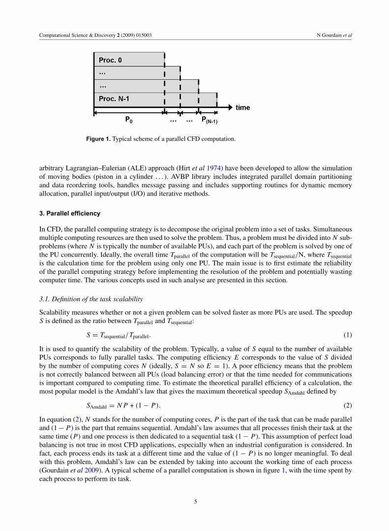
Figure 1. Typical scheme of a parallel CFD computation.

arbitrary Lagrangian–Eulerian (ALE) approach (Hirt et al 1974) have been developed to allow the simulationof moving bodies (piston in a cylinder . . . ). AVBP library includes integrated parallel domain partitioningand data reordering tools, handles message passing and includes supporting routines for dynamic memoryallocation, parallel input/output (I/O) and iterative methods.

3. Parallel efficiency

In CFD, the parallel computing strategy is to decompose the original problem into a set of tasks. Simultaneousmultiple computing resources are then used to solve the problem. Thus, a problem must be divided into N sub-problems (where N is typically the number of available PUs), and each part of the problem is solved by one ofthe PU concurrently. Ideally, the overall time Tparallel of the computation will be Tsequential/N, where Tsequential

is the calculation time for the problem using only one PU. The main issue is to first estimate the reliabilityof the parallel computing strategy before implementing the resolution of the problem and potentially wastingcomputer time. The various concepts used in such analyse are presented in this section.

3.1. Definition of the task scalability

Scalability measures whether or not a given problem can be solved faster as more PUs are used. The speedupS is defined as the ratio between Tparallel and Tsequential:

S = Tsequential/Tparallel. (1)

It is used to quantify the scalability of the problem. Typically, a value of S equal to the number of availablePUs corresponds to fully parallel tasks. The computing efficiency E corresponds to the value of S dividedby the number of computing cores N (ideally, S = N so E = 1). A poor efficiency means that the problemis not correctly balanced between all PUs (load balancing error) or that the time needed for communicationsis important compared to computing time. To estimate the theoretical parallel efficiency of a calculation, themost popular model is the Amdahl’s law that gives the maximum theoretical speedup SAmdahl defined by

SAmdahl = N P + (1 − P). (2)

In equation (2), N stands for the number of computing cores, P is the part of the task that can be made paralleland (1 − P) is the part that remains sequential. Amdahl’s law assumes that all processes finish their task at thesame time (P) and one process is then dedicated to a sequential task (1 − P). This assumption of perfect loadbalancing is not true in most CFD applications, especially when an industrial configuration is considered. Infact, each process ends its task at a different time and the value of (1 − P) is no longer meaningful. To dealwith this problem, Amdahl’s law can be extended by taking into account the working time of each process(Gourdain et al 2009). A typical scheme of a parallel computation is shown in figure 1, with the time spent byeach process to perform its task.

5


(a) (b)

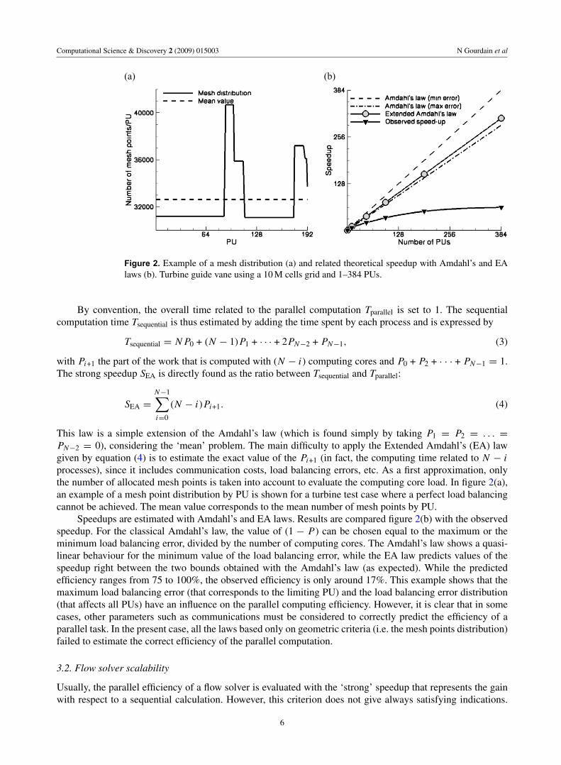
Figure 2. Example of a mesh distribution (a) and related theoretical speedup with Amdahl’s and EAlaws (b). Turbine guide vane using a 10 M cells grid and 1–384 PUs.

By convention, the overall time related to the parallel computation Tparallel is set to 1. The sequentialcomputation time Tsequential is thus estimated by adding the time spent by each process and is expressed by

Tsequential = N P0 + (N − 1)P1 + · · · + 2PN−2 + PN−1, (3)

with Pi+1 the part of the work that is computed with (N − i) computing cores and P0 + P2 + · · · + PN−1 = 1.The strong speedup SEA is directly found as the ratio between Tsequential and Tparallel:

SEA =

N−1∑i=0

(N − i)Pi+1. (4)

This law is a simple extension of the Amdahl’s law (which is found simply by taking P1 = P2 = . . . =

PN−2 = 0), considering the ‘mean’ problem. The main difficulty to apply the Extended Amdahl’s (EA) lawgiven by equation (4) is to estimate the exact value of the Pi+1 (in fact, the computing time related to N − iprocesses), since it includes communication costs, load balancing errors, etc. As a first approximation, onlythe number of allocated mesh points is taken into account to evaluate the computing core load. In figure 2(a),an example of a mesh point distribution by PU is shown for a turbine test case where a perfect load balancingcannot be achieved. The mean value corresponds to the mean number of mesh points by PU.

Speedups are estimated with Amdahl’s and EA laws. Results are compared figure 2(b) with the observedspeedup. For the classical Amdahl’s law, the value of (1 − P) can be chosen equal to the maximum or theminimum load balancing error, divided by the number of computing cores. The Amdahl’s law shows a quasi-linear behaviour for the minimum value of the load balancing error, while the EA law predicts values of thespeedup right between the two bounds obtained with the Amdahl’s law (as expected). While the predictedefficiency ranges from 75 to 100%, the observed efficiency is only around 17%. This example shows that themaximum load balancing error (that corresponds to the limiting PU) and the load balancing error distribution(that affects all PUs) have an influence on the parallel computing efficiency. However, it is clear that in somecases, other parameters such as communications must be considered to correctly predict the efficiency of aparallel task. In the present case, all the laws based only on geometric criteria (i.e. the mesh points distribution)failed to estimate the correct efficiency of the parallel computation.

3.2. Flow solver scalability

Usually, the parallel efficiency of a flow solver is evaluated with the ‘strong’ speedup that represents the gainwith respect to a sequential calculation. However, this criterion does not give always satisfying indications.

6


(a) (b)

Figure 3. Overview of the normalized speedup for applications with elsA (a) and AVBP (b).

Firstly, a good speedup can be related to poor sequential performance (for example, if a PU computes slowlywith respect to its communication network). This point is critical, especially for cached-based processors:super-linear speedups are often observed in the literature with these chips, mainly because the large amountof data required by the flow solver leads to a drop down of the processor performance for a sequential task.For CFD applications, the potential solution is to increase the size of the cache memory and to reduce thecommunication time between the different cache levels. Secondly, the sequential time is usually not known,mainly due to limited memory resources. Except for vector supercomputer, the typical memory size availablefor one PU ranges from 512 Mb to 32 Gb. As a consequence, in most cases, industrial configurations cannot berun on scalar platforms with a single computing core and no indication about the real speedup can be obtained.A common definition of the speedup is often used by opposition to the ‘strong’ speedup: the normalizedspeedup that is related to the time ratio between a calculation with N PUs and Nmin PUs, where Nmin is thesmallest number of PUs that can be used for the application. The normalized speedup is thus useful to give anidea of the flow solver scalability.

A short overview of the normalized speedup obtained for many applications performed with elsA andAVBP is indicated in figure 3. While elsA shows a good scalability until 2048 PUs, results for 4096 PUs arequite disappointing.

This is mainly related to the difficulty for balancing a complex geometry configuration (non-coincidentinterfaces between blocks). Moreover, the load balancing error can be modified during this unsteady flowsimulation (due to sliding mesh). AVBP has a long experience in massively parallel calculations, as indicatedby the wide range of scalar supercomputers used. This flow solver shows an excellent scalability until 6144PUs since the normalized speedup is very close to ideal. Results are still good for 12 288 PUs (efficiencyis around 77%). This decrease of performance for a very large number of PUs underlines a physical limitoften encountered on massively parallel applications. Indeed for very large numbers of PUs the ratio betweencomputation time and communication time is directly proportional to the problem size (number of gridpoints and unknowns). For this specific illustration, the configuration tested with 12 288 PUs corresponds toa calculation with less than 3000 cells by PU or a too low computational workload for each PU compared tothe amount of exchanges needed to proceed with the CFD computation. It shows that a given task is limited interms of scalability and no increase of performance is expected beyond a given number of PUs.

4. Mesh partitioning strategies

The mesh partitioning is thus a challenging step to maintain good efficiency as the number of computing coresincreases. Many claims of ‘poor parallel scaling’ are often ill-found, and usually vanish if care is brought to

7


(a)

(b)

Figure 4. Overview of the mesh partitioning strategies: (a) pre-processing step with a SPMD approachand (b) dynamic mesh-partitioning with a MPMD approach.

ensure good load balancing and minimization of overall communication time. Indeed, the possibility to runa problem on a large number of PUs is related to the capacity of efficiently splitting the original probleminto parallel sub-domains. The original mesh is partitioned in several sub-domains that are then (ideallyequally) distributed between all PUs. One of the limitations is that the use of parallel partitioning algorithmsoften needed when using many computing cores remains very complex and this task is usually performedsequentially by one PU, leading to memory constraints. These constraints are much more important forunstructured meshes than for block-structured meshes, mainly because the mesh-partitioning of unstructuredgrids requires large tables for mesh coordinates and connectivity.

4.1. General organization

In most flow solvers, mesh partitioning is done in three steps: graph partitioning, nodes (re)ordering and blocksgeneration. An additional step is the merging of output data generated by each subtask (useful in an industrialcontext for data visualization and post-processing). As shown in figure 4, two strategies can be used: either

8


(a) (b)

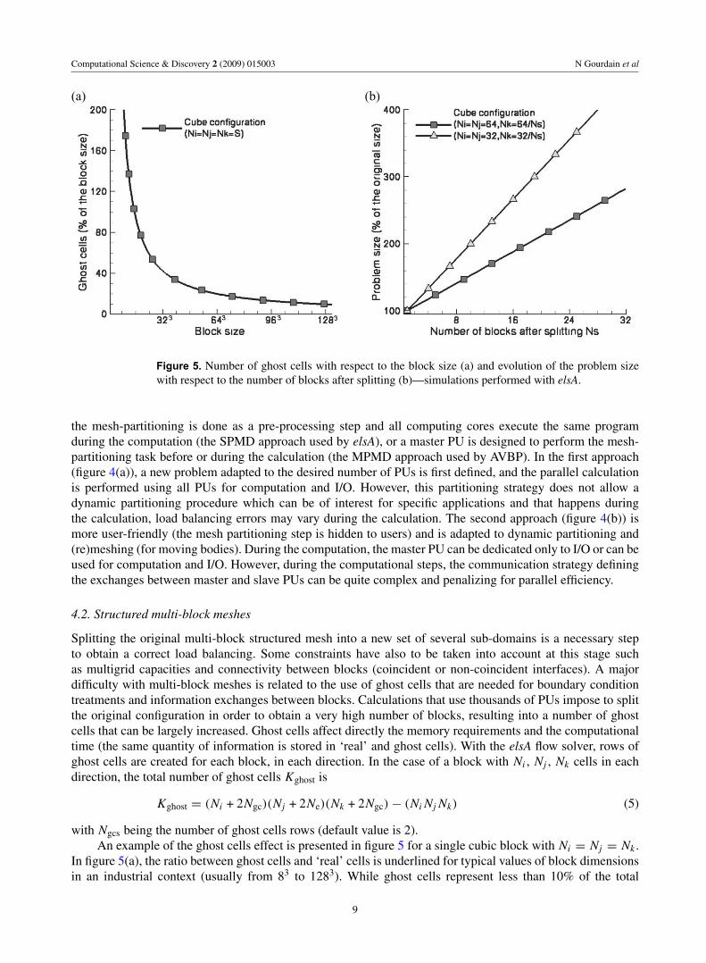
Figure 5. Number of ghost cells with respect to the block size (a) and evolution of the problem sizewith respect to the number of blocks after splitting (b)—simulations performed with elsA.

the mesh-partitioning is done as a pre-processing step and all computing cores execute the same programduring the computation (the SPMD approach used by elsA), or a master PU is designed to perform the mesh-partitioning task before or during the calculation (the MPMD approach used by AVBP). In the first approach(figure 4(a)), a new problem adapted to the desired number of PUs is first defined, and the parallel calculationis performed using all PUs for computation and I/O. However, this partitioning strategy does not allow adynamic partitioning procedure which can be of interest for specific applications and that happens duringthe calculation, load balancing errors may vary during the calculation. The second approach (figure 4(b)) ismore user-friendly (the mesh partitioning step is hidden to users) and is adapted to dynamic partitioning and(re)meshing (for moving bodies). During the computation, the master PU can be dedicated only to I/O or can beused for computation and I/O. However, during the computational steps, the communication strategy definingthe exchanges between master and slave PUs can be quite complex and penalizing for parallel efficiency.

4.2. Structured multi-block meshes

Splitting the original multi-block structured mesh into a new set of several sub-domains is a necessary stepto obtain a correct load balancing. Some constraints have also to be taken into account at this stage suchas multigrid capacities and connectivity between blocks (coincident or non-coincident interfaces). A majordifficulty with multi-block meshes is related to the use of ghost cells that are needed for boundary conditiontreatments and information exchanges between blocks. Calculations that use thousands of PUs impose to splitthe original configuration in order to obtain a very high number of blocks, resulting into a number of ghostcells that can be largely increased. Ghost cells affect directly the memory requirements and the computationaltime (the same quantity of information is stored in ‘real’ and ghost cells). With the elsA flow solver, rows ofghost cells are created for each block, in each direction. In the case of a block with Ni , Nj , Nk cells in eachdirection, the total number of ghost cells Kghost is

Kghost = (Ni + 2Ngc)(Nj + 2Ne)(Nk + 2Ngc) − (Ni Nj Nk) (5)

with Ngcs being the number of ghost cells rows (default value is 2).An example of the ghost cells effect is presented in figure 5 for a single cubic block with Ni = Nj = Nk .

In figure 5(a), the ratio between ghost cells and ‘real’ cells is underlined for typical values of block dimensionsin an industrial context (usually from 83 to 1283). While ghost cells represent less than 10% of the total

9


Figure 6. Evolution of the problem size and number of blocks after splitting for an industrialcompressor configuration (elsA, greedy algorithm).

size of a block with 1283 cells, the value reaches more than 40% for a block with 323 cells. For very smallblocks typically used for technological effects (such as thick trailing edge, tails, tip leakage, etc), the numberof ghost cells could be more than 200% of the number of ‘real’ cells. The effect of block splitting on ghostcells is pointed out by figure 5(b). It clearly shows the increase of the problem size after successive blockssplitting, for two initial block sizes (643 and 323). The law followed by the problem size is perfectly linearwith a slope that depends only on the original block size. If an initial block with 643 cells is split into 16new blocks of equal dimensions, the problem size has been increased by 190%. An example of the meshsplitting impact on industrial applications is shown in figure 6. The configuration is an industrial multi-stagecompressor represented by an original grid composed of 2848 blocks and more than 130 millions cells. Theoriginal configuration is split and balanced over 512 PUs to 12 288 PUs. As expected, the number of blocksand the size of the problem are directly correlated. For a reasonable number of PUs, the number of ghost cellshas a relatively small impact on the size of the problem while the number of blocks is largely increased withrespect to the original configuration. For example, the size of the configuration corresponding to 4096 PUs isincreased by +8% while the number of blocks is increased by +210%. In fact, only largest blocks have beensplit, leading to a small impact on the number of ghost cells. However, for 12 288 PUs, both the number ofblocks and the size of the configuration are significantly increased (respectively +590% and +37%s). It is clearthat this problem come from the use of ghost cells, which is not adapted to massively parallel calculationswhen block splitting is required. On the one hand, the suppression of this method would result in an increaseof the parallel efficiency. On the other hand it will also considerably increase the sequential time. Indeed, thebalance between both effects is not easy to predict and the result will depend on the configuration and thenumber of desired PUs.

For parallel computing applications, the program allocates one or more blocks to each PU with theobjective of minimizing the load balancing error. To evaluate the load of PUs, the elsA software considersonly the total number of cells Qtotal (ghost cells are not taken into account). Then the ideal number of cellsQmean allocated to one computing core depends only on the total number of computing cores N :

Qmean =Qtotal

N. (6)

The load balancing error related to a given PU is defined as the relative error between the allocated numberof cells and the ideal number of cells Qmean which would result into an optimal work load of the PU. Theobjective of mesh partitioning is to minimize the load balancing error. Two mesh partitioning algorithmsare available in elsA that only consider geometric information (no information from the communicationgraph is used):

10


Figure 7. Example of a multi-block mesh partitioning and load balancing with the greedy algorithm(elsA calculations).

• The recursive edge bisection (REB) algorithm works only on the largest domain (it splits the largest blockalong its longest edge until the number of blocks equals the desired number of PUs indicated by the user).This very simple algorithm is well adapted to simple geometries such as cubes but it usually gives poorquality results in complex configurations;

• The so-called greedy algorithm is a more powerful tool to split blocks and is based only on geometriccriteria (Ytterström 1997). This approach loops over blocks looking for the largest one (after splittingwhen necessary) and allocating it to the PU with the smaller number of cells until all blocks are allocated.An example is shown in figure 7 for a configuration with five initial blocks. Based on an objective of 16PUs, the greedy algorithm successively splits the blocks to obtain a new problem with 19 blocks yieldinga load balancing error of roughly 3%.

It is known that the problem of finding the optimal set of independent edges is NP-complete (i.e. it is a non-polynomial and non-deterministic problem). More information about NP-complete problem can be found inGarey and Johnson (1979). With a few hundred computing cores, the greedy heuristic approach gives goodresults and more sophisticated methods would probably not significantly improve the graph coverage (Gazaixet al 2008). However, for applications with thousands of PUs, some improvements should be considered.A simple thing to do is to order the edges according to their weight (based on the size of the interface meshes).In this case, the edge weights in one set are close to each other, and every message in one communicationstage should take approximately the same amount of time to exchange. This method is expected to reduce thecommunication time.

4.3. Unstructured meshes

An example of an unstructured grid and its associated dual graph are shown in figure 8(a). Each vertexrepresents a finite element of the mesh and each edge represents a connexion between the faces of twoelements (and therefore, the communication between adjacent mesh elements). The number of edges of thedual graph that are being cut by partitioning is called an edge-cut. This subdivision results in an increase ofthe total number of grid points due to a duplication of nodes at the interface between two sub-domains. Thecommunication cost of a sub-domain is a function of its edge-cut as well as the number of neighbouring sub-domains that share edges with it. In practice, the edge-cut of a partitioning is used as an important indicatorof partitioning quality for cell-vertex codes. The sparse matrix related to the dual graph of this grid is shownin figure 8(b). The axes represent the vertices in the graph and the black squares show an edge betweenvertices. For CFD applications, the order of the elements in the sparse matrix usually affects the performanceof numerical algorithms. The objective is to minimize the bandwidth of the sparse matrix (which represents

11


(a) (b)

Figure 8. Example of an unstructured grid with its associated dual graph and partitioning process (a)and the related sparse matrix (b).

Figure 9. Effect of the nodes ordering on the computational efficiency of AVBP. CM and RCM showan increase of the efficiency by +35%.

the problem to solve) by renumbering the nodes of the computational mesh in such a way that they are asclose as possible to their neighbours. This insures optimal use of memory of the computational resources andis mandatory in unstructured CFD solvers. In AVBP, node reordering can be done by the Cuthill–McKee (CM)or the reverse Cuthill–McKee (RCM) algorithms (Cuthill and McKee 1969). In the case of AVBP, the RCMalgorithm provides similar results at a lower cost in terms of time than the CM algorithm. An example of theeffects of node reordering on the performance of a simulation with AVBP is presented in figure 9.

The configuration used in these tests is a hexahedron-based grid with 3.2 millions of nodes (and3.2 millions cells). The impact of nodes ordering is measured through the computational efficiency, defined asthe ratio between the computational time after reordering and before reordering. With 32 PUs, this efficiencyincreases by +35% with the CM or the RCM methods. These results show the importance of nodes ordering,in the case of unstructured CFD solvers especially on massively parallel machines to simulate large scaleindustrial problems. Different partitioning algorithms are currently available in AVBP and largely detailed

12


Figure 10. Example of a partitioning process with an unstructured grid and the RIB algorithm (AVBPcalculations).

in Garcia (2009). Two methods are geometric based algorithms, considering only coordinates and distancesbetween nodes (Euclidean distance). A third one is a graph theory based algorithm that uses the graphconnectivity information. These three first algorithms give satisfactory results for most applications but showlimitations in terms of computational time and mesh partitioning quality for large size problems (such as theone usually considered with HPC). A fourth algorithm has thus been implemented (METIS) in AVBP (Karypisand Kumar 1998), which is especially well adapted for Lagrangian and massively parallel calculations. A shortdescription of these four methods is provided below.

• Recursive coordinate bisection (RCB) is equivalent to the REB algorithm available in the elsA software(Berger and Bokhari 1987). The weakness of this algorithm is that it does not take advantage of theconnectivity information.

• Recursive inertial bisection (RIB) is similar to RCB (Williams 1991) but it provides a solution that doesnot depend on the initial mesh orientation (figure 10). The weakness of this algorithm is identical to theRCB method.

• Recursive graph bisection (RGB) considers the graph distance between two nodes (Simon 1991). InAVBP, the determination of pseudo-peripheral nodes, which is critical for the algorithm, is obtained withthe Lewis implementation of the Gibbs–Poole–Stockmeyer algorithm (Lewis 1982). The interest of thismethod is that it considers the graph distance.

• The METIS algorithms are based on multilevel graph partitioning: multilevel recursive bisectioning(Karypis and Kumar 1999) and multilevel k-way partitioning (Karypis and Kumar 1998). As thepartitioning algorithms operate with a reduced-size graph (figure 11), they are extremely fast comparedto traditional partitioning algorithms. Testing has also shown that the partitions provided by METIS areusually better than those produced by other multilevel algorithms (Hendrickson and Leland 1993).

It is not always easy to choose the best partitioning algorithm for a given scenario. The quality of the partitionand the time to perform it are two important factors to estimate the performance of a partitioning algorithm.Complex simulations such as Euler–Lagrange calculations (two-phase flows) are good candidates to evaluatemesh partitioning algorithms (Apte et al 2003). During a two-phase flow simulation, particles are free tomove everywhere in the calculation domain. As a first approximation, it is possible to assume that the particledensity is constant in the domain. In this case, the number of particles in a domain depends only on thedomain dimension (a large volume corresponds to a high number of particles). Results obtained with twodifferent algorithms are presented in figure 12. The RCB algorithm takes into account only information relatedto the number of cells while the k-way algorithm (METIS) uses more constraints such as particle density.A comparison of the two methods shows that the RCB method leads to an incorrect solution for load balancing(figure 13). With the RCB algorithm one PU supports the calculation for most the particles, figure 13(a). Thek-way algorithm gives a more satisfactory result by splitting the mesh in more reasonable dimensions, leadingto a correct load balancing of the particles between PUs, figure 13(b). Many tests have been performed witha wide range of sub-domain numbers, from 64 (26) to 16 384 (214), in order to evaluate the scalability of

13


Figure 11. Working scheme of the multilevel graph bisection. During the uncoarsening phase thedotted lines indicate projected partitions and solid lines indicate partitions after refinement (Karypisand Kumar 1999).

Figure 12. Example of the mesh partitioning considering a two-phase flow configuration with AVBP(a) by using the RCB algorithm (b) and the k-way algorithm used by METIS (c).

the different partitioning algorithms. The time required to partition a grid of 44 millions cells on 4096 sub-domains ranges from 25 min with METIS (k-way algorithm) to 270 min with the RGB algorithm (benchmarksperformed on an Opteron-based platform).

For most applications, METIS gives the fastest results, except for small size grids and for large numberof PUs (for which the RCB algorithm is slightly better). To compare the quality of the mesh partitioning, thenumber of nodes after partitioning is shown in figure 14 for moderate (10 millions cells, 1.9 millions nodes)and large (44 millions cells, 7.7 millions nodes) grids. The reduction in the number of nodes duplicated with thek-way algorithm of METIS is significant. The difference tends to be larger when the number of sub-domains

14


(a) RCB algorithm

(b) k-way algorithm (METIS)

Figure 13. Impact of the mesh-partitioning on the particle balance with AVBP: (a) RCB algorithm and(b) k-way algorithm (METIS).

(a) (b)

Figure 14. Number of nodes after partitioning of combustion chamber meshes with AVBP by usingRCB and k-way (METIS) methods: grids with 10 millions (a) and 44 million cells (b).

increases, leading to an important gain in the calculation efficiency due to the reduction of the number of nodesand communication costs.

The previous example shows that a considerable improvement of the mesh-partitioning quality canbe obtained by using multi-levels and multi-graphs algorithms. In fact for AVBP, the combination of theRCM algorithm (for node reordering) and the METIS algorithms provide the best results in terms of

15


cost/parallel efficiency ratio. Moreover, these algorithms usually provide a solution in a less amount of timethan classical geometrical algorithms and they are particularly well fitted to parallel implementation. Indeed,the development of a parallel implementation for partitioning algorithms is a current challenge to reduce thecomputational cost of this step.

5. Communication and scheduling

For most CFD applications, processes are not fully independent and data exchange is required at some points(fluxes at block interfaces, residuals, etc). The use of an efficient strategy for message passing is thus necessaryfor parallel computing, especially with a large number of computing cores. Specific instructions are giventhrough standard protocols to communicate data between computing cores, such as message passing interface(MPI) and OpenMP. Communication, message scheduling and memory bandwidth effects are detailed in thissection.

5.1. Presentation of message passing protocols

MPI is a message passing standard library based on the consensus of the MPI Forum (more than 40participating organizations). Different kinds of communication can be considered in the MPI applicationprogram interface (API) such as point-to-point and collective communications (Gropp et al 1999). Point-to-point MPI calls are related to data exchange between only two specific processes (such as the MPI‘send’ function family). Collective MPI calls involve communication between all computing cores in a group(either the entire process pool or a user-defined subset). Each of these communications can be done through‘blocking’ (the program execution is suspended until the message buffer is safe to use) or ‘non-blocking’protocols (the program does not wait to be certain that the communication buffer is safe to use). Non-blocking communications have the advantage of allowing the computation to proceed immediately after theMPI communication call (computation and communication can be overlapping). While MPI is currently themost popular protocol for CFD flow solvers, it is not perfectly well adapted to new computing architectureswith greater internal concurrency (multi-core) and more levels of memory hierarchy. Multithreaded programscan potentially take advantage of these developments more easily than single threaded applications. Thishas already led to separate, complementary standards for symmetric multiprocessing, such as the OpenMPprotocol. The OpenMP API supports multi-platform shared-memory parallel programming in C/C ++ andFortran on all architectures. The OpenMP communication system is based on the fork-join scheme withone master thread (i.e. a series of instructions executed consecutively) and working threads in the parallelregion. More information about OpenMP can be found in Chapman et al (2007). Advantages of OpenMPare simplicity since programmer does not need to deal with message passing (needed with MPI) and allowsan incremental parallelism approach (user can choose on which part of the program OpenMP is used withoutdramatic changes inside the code). However, the main drawbacks are that it runs only in shared-memory multi-cores platforms and scalability is limited by memory architecture. Today most CFD calculations require morethan one computing node hosting few PUs, meaning OpenMP is still not sufficient to parallelize efficiently aflow solver aimed for massive industrial and realistic problems.

5.2. Blocking and non-blocking message passing interface communications

Communications in AVBP and elsA can be implemented either through MPI blocking calls or MPI non-blocking calls. MPI non-blocking is a good way to reduce the communication time with respect to blockingMPI calls but it also induces a non-deterministic behaviour that participates to rounding errors (for exampleresiduals are computed following a random order). To overcome this problem, a solution is to use MPI blockingcalls with a scheduler. The objective is to manage the ordering of communication for minimizing the globalcommunication time. Such a strategy has been tested in elsA. As shown in figure 15, the scheduling of blockingMPI communications is based on a heuristic algorithm that uses a weighted multi-graph. The graph verticesrepresent the available PUs and therefore an edge connects two cores. An edge also represents a connectivitythat links two sub-domains. A weight is associated with each edge, depending on the number of connection

16


Figure 15. Simplified example of a multi-graph used for the scheduling process in elsA.

interfaces (cell faces). Since many sub-domains (i.e. block in the case of elsA) can be assigned to only onePU, two vertices of the graph can be connected with many edges, hence the name multi-graph. The underlyingprinciple of the ordering algorithm is to structure the communication scheme into successive message passingstages. Indeed, the communication scheme comes into play at some steps during an iteration of the solver,whenever sub-domains need information from their neighbours. A message passing stage represents thereforea step where all PUs are active, which means that they are not waiting for other processes but are insteadconcerned by message passing. Each communication stage is represented by a list containing the graph edgesthat have no process in common. In other words, if one edge is taken from this list, then PUs related to thecorresponding vertices will not appear in other edges. The load-balancing process must ensure that all PUssend nearly the same number of messages (with the same size) so the scheduler can assign the same numberof communication stages to them.

Benchmarks have been performed with the structured flow solver elsA to quantify the influence of theMPI implementation on the point-to-point communications (coincident interfaces). In the current version ofthe flow solver, each block connectivity is implemented with the instruction ‘MPI Sendrecv replace()’. Thisapproach is compared with a non-blocking communication scheme that uses the ‘MPI Irecv’ and ‘MPI Isend’instructions. Both implementations have been tested with and without the scheduler. The computationalefficiency obtained with an IBM Blue Gene/L platform for a whole aircraft configuration (30 M cells gridand 1774 blocks) is indicated in figure 16. The reference used is the computational time observed with thestandard blocking MPI instructions. As it can be seen, when the scheduler is used there is no difference in theefficiency with respect to the standard MPI implementation. However, without the scheduler, the computationalefficiency with the blocking MPI implementations is reduced by 40% while no effect is observed with a non-blocking implementation.

These benchmarks clearly indicate that both implementations provide identical performance regardingthe communication efficiency, at least for point-to-point communications. However, a scheduling step isrequired to ensure a good computing efficiency with MPI blocking calls. Particular care is necessary whenthe configuration is split to minimize the number of communications stages. The maximum degree of thegraph used for scheduling is the minimum number of communication stages that may take place. It is thusimportant to limit the ratio between the maximum and minimum degrees of the graph vertices that indicatesthe rate of idleness of the computing core.

5.3. Point-to-point and collective message passing interface communications

Communications can also be done by using point-to-point communications and/or collective MPI calls. Inthe case of elsA, both methods are used: the first one for coincident interfaces and the second one fornon-coincident interfaces. The strategy is thus to treat first the point-to-point communication and then thecollective communications. As a consequence, if non-coincident interfaces are not correctly shared betweenall computing cores, a group of cores will wait for the cores interested by the collective MPI calls (it is alsotrue for point-to-point communications). An example of the communications ordering obtained on an IBM

17


Figure 16. Effect of the MPI implementation on the code efficiency (benchmarks are performed withelsA on an IBM Blue Gene/L platform).

Figure 17. Communication scheduling for one iteration with elsA on a Blue Gene/L system (N =

4096 PUs)—each line corresponds to one PU, black is related to point-to-point communications andgrey to collective communications.

Blue Gene /L system with the MPI Trace library is shown in figure 17. From left to right, time corresponds toone iteration of the flow solver (with an implicit scheme). The configuration is a multistage compressor thatrequires both coincident and non-coincident interfaces between blocks. The calculation has been performedwith 4096 PUs but for clarity, data of figure 17 is presented only for 60 PUs (each line of the graph correspondsto one PU). The white region is related to the computation work while grey and black regions correspondto MPI calls. The collective communications are highlighted (in grey) and appear after the point-to-pointones (in black). The graph indicates how the management of these communications can reduce the parallel

18


(a) (b)

Figure 18. Evolution of the number of cells by computing core (a) and effect of the communicationstrategy on the scalability (b) of AVBP (SGI Altix platform).

computing efficiency. MPI calls are related to the necessity for exchanging information, such as auxiliaryquantities (gradients, etc) at the beginning of the iteration or the increments of conservative variables 1Wi

during the implicit stages. At the end of the iteration, all the PUs exchange the conservative variables W andresiduals RW , using collective calls. In figure 17, two groups of processes are identified: group 1 is linked tocoincident and non-coincident interfaces while group 2 is linked only to coincident interfaces. For example,when auxiliary quantities are exchanged, while group 1 is still doing collective MPI calls, group 2 has alreadystarted to compute fluxes. However, during the implicit calculation, all processes have to be synchronized toexchange 1Wi . This explains why the point-to-point communication related to group 2 appears so long: allthe PUs associated with group 2 cannot continue their work and are waiting for the PUs of group 1. In thisexample, collective MPI calls are not correctly balanced, increasing the communication time.

In the unstructured flow solver AVBP, all communications between PUs are implemented throughMPI non-blocking communications. AVBP does not use directly the syntax of the MPI library, but ratheremploys the integrated parallel macros (IPM) library developed at CERFACS (Giraud 1995) that acts as anintermediate layer to switch between different parallel message passing libraries. To highlight the role ofcommunications, both point-to-point and collective calls have been tested. With point-to-point communication,all slave processes first send information to the master and then the master returns a message to all slaveprocesses. It leads to the exchange of 2N messages (with N the total number of PUs). With collective callscommunications, all processes have to exchange only 2ln(N) messages. The second strategy minimizes theamount of information to exchange between computing cores through the network. Tests have been performedfor a combustion chamber configuration up to 8192 PUs on a distributed shared memory supercomputer (SGIAltix, Harpertown cores). The grid of the test case is composed of 75 millions cells. The number of cells percomputing core and the observed speedup are indicated in figures 18(a) and (b), respectively.

The communication strategy has a very small impact until 2048 PUs. When a higher number of PUsis used, the strategy based on point-to-point communication leads to a dramatic reduction of the parallelefficiency: the maximum speedup is observed with 4096 PUs before decreasing to 1500 with 8192 PUs. Incontrast, with a collective MPI communication, the speedup is almost linear (with 8192 PUs, the speedup isaround 7200, i.e. an efficiency nearly 90%). With 2048 and 4096 PUs, the observed speedups are even higherthan the linear law. This observation can be explained by the cache memory behaviour (PUs have a very fastaccess to data stored in a small private memory). When the problem is split into subtasks, the size of this datais reduced and it can thus be stored in this memory, explaining why calculations are sometimes more efficient

19


(a) (b)

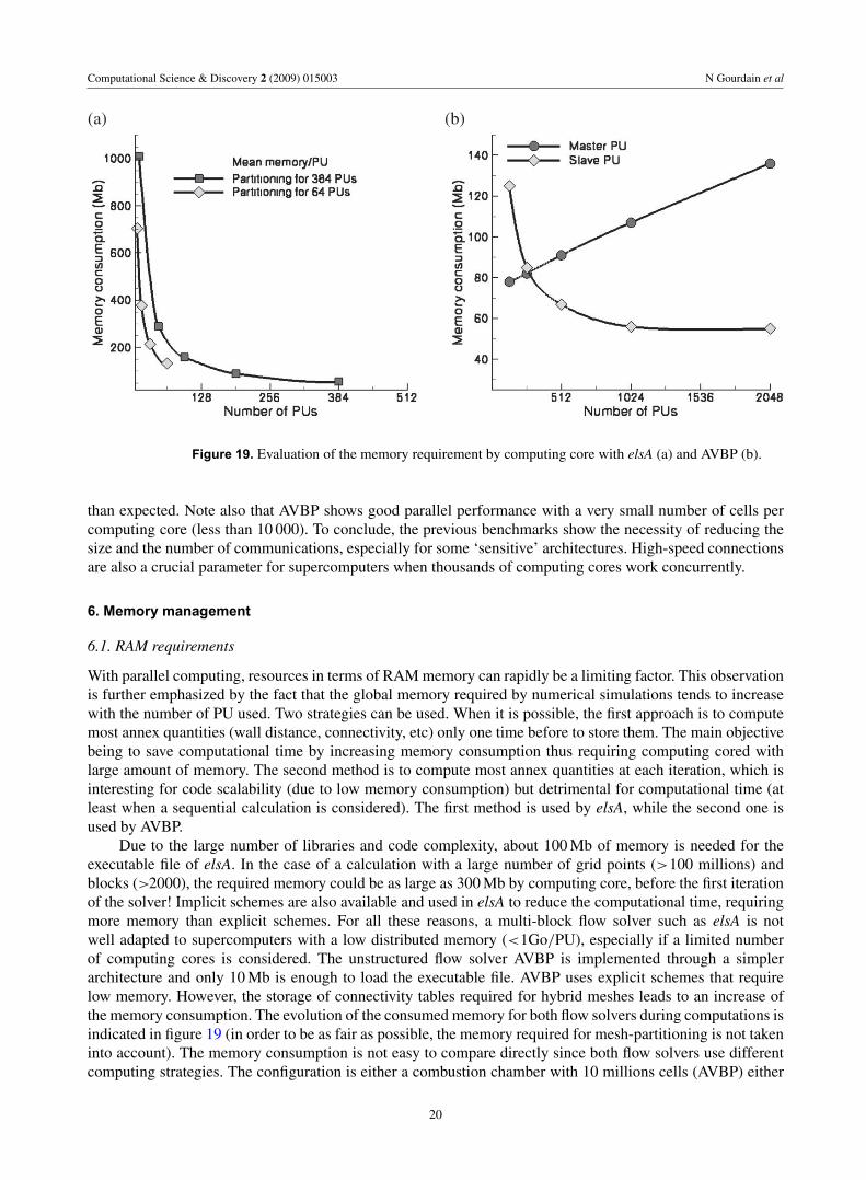
Figure 19. Evaluation of the memory requirement by computing core with elsA (a) and AVBP (b).

than expected. Note also that AVBP shows good parallel performance with a very small number of cells percomputing core (less than 10 000). To conclude, the previous benchmarks show the necessity of reducing thesize and the number of communications, especially for some ‘sensitive’ architectures. High-speed connectionsare also a crucial parameter for supercomputers when thousands of computing cores work concurrently.

6. Memory management

6.1. RAM requirements

With parallel computing, resources in terms of RAM memory can rapidly be a limiting factor. This observationis further emphasized by the fact that the global memory required by numerical simulations tends to increasewith the number of PU used. Two strategies can be used. When it is possible, the first approach is to computemost annex quantities (wall distance, connectivity, etc) only one time before to store them. The main objectivebeing to save computational time by increasing memory consumption thus requiring computing cored withlarge amount of memory. The second method is to compute most annex quantities at each iteration, which isinteresting for code scalability (due to low memory consumption) but detrimental for computational time (atleast when a sequential calculation is considered). The first method is used by elsA, while the second one isused by AVBP.

Due to the large number of libraries and code complexity, about 100 Mb of memory is needed for theexecutable file of elsA. In the case of a calculation with a large number of grid points (>100 millions) andblocks (>2000), the required memory could be as large as 300 Mb by computing core, before the first iterationof the solver! Implicit schemes are also available and used in elsA to reduce the computational time, requiringmore memory than explicit schemes. For all these reasons, a multi-block flow solver such as elsA is notwell adapted to supercomputers with a low distributed memory (<1Go/PU), especially if a limited numberof computing cores is considered. The unstructured flow solver AVBP is implemented through a simplerarchitecture and only 10 Mb is enough to load the executable file. AVBP uses explicit schemes that requirelow memory. However, the storage of connectivity tables required for hybrid meshes leads to an increase ofthe memory consumption. The evolution of the consumed memory for both flow solvers during computations isindicated in figure 19 (in order to be as fair as possible, the memory required for mesh-partitioning is not takeninto account). The memory consumption is not easy to compare directly since both flow solvers use differentcomputing strategies. The configuration is either a combustion chamber with 10 millions cells (AVBP) either

20


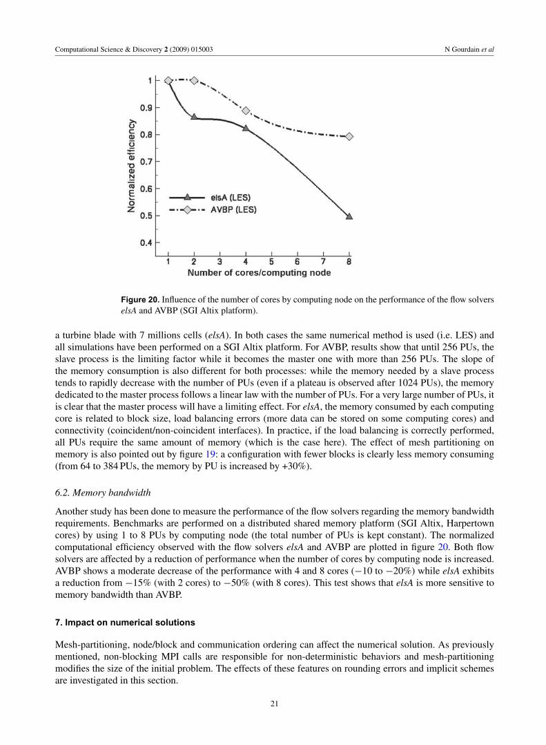
Figure 20. Influence of the number of cores by computing node on the performance of the flow solverselsA and AVBP (SGI Altix platform).

a turbine blade with 7 millions cells (elsA). In both cases the same numerical method is used (i.e. LES) andall simulations have been performed on a SGI Altix platform. For AVBP, results show that until 256 PUs, theslave process is the limiting factor while it becomes the master one with more than 256 PUs. The slope ofthe memory consumption is also different for both processes: while the memory needed by a slave processtends to rapidly decrease with the number of PUs (even if a plateau is observed after 1024 PUs), the memorydedicated to the master process follows a linear law with the number of PUs. For a very large number of PUs, itis clear that the master process will have a limiting effect. For elsA, the memory consumed by each computingcore is related to block size, load balancing errors (more data can be stored on some computing cores) andconnectivity (coincident/non-coincident interfaces). In practice, if the load balancing is correctly performed,all PUs require the same amount of memory (which is the case here). The effect of mesh partitioning onmemory is also pointed out by figure 19: a configuration with fewer blocks is clearly less memory consuming(from 64 to 384 PUs, the memory by PU is increased by +30%).

6.2. Memory bandwidth

Another study has been done to measure the performance of the flow solvers regarding the memory bandwidthrequirements. Benchmarks are performed on a distributed shared memory platform (SGI Altix, Harpertowncores) by using 1 to 8 PUs by computing node (the total number of PUs is kept constant). The normalizedcomputational efficiency observed with the flow solvers elsA and AVBP are plotted in figure 20. Both flowsolvers are affected by a reduction of performance when the number of cores by computing node is increased.AVBP shows a moderate decrease of the performance with 4 and 8 cores (−10 to −20%) while elsA exhibitsa reduction from −15% (with 2 cores) to −50% (with 8 cores). This test shows that elsA is more sensitive tomemory bandwidth than AVBP.

7. Impact on numerical solutions

Mesh-partitioning, node/block and communication ordering can affect the numerical solution. As previouslymentioned, non-blocking MPI calls are responsible for non-deterministic behaviors and mesh-partitioningmodifies the size of the initial problem. The effects of these features on rounding errors and implicit schemesare investigated in this section.

21


Figure 21. Effect of mesh-partitioning on the convergence level with implicit schemes (unsteady flowsimulation performed with elsA).

7.1. Mesh-partitioning and implicit algorithms

Implicit stage done on a block basis (such as in elsA) is a difficulty for mesh-partitioning. Block splittingperformed to achieve good load balancing may reduce the numerical efficiency of the implicit algorithm.Simulations of the flow in a high-pressure turbine have been performed (without block splitting) with differentnumbers of PUs, using RANS then LES. For both elsA tests, no difference is observed on the instantaneoussolutions and convergence is strictly identical. A second set of simulation is performed by considering thesame test case but with different mesh partitioning keeping an identical number of PUs. The unsteady RANSflow simulation is performed with elsA and results of tests are shown in figure 21. No significant differenceon the convergence level between both configurations is observed until a normalized time of t+

= 10. Aftert+

= 10, although convergence levels are of the same order, differences are observed on the instantaneousresiduals. In practice, no significant degradation on convergence level has ever been reported.

7.2. Rounding errors and large eddy simulation

The effect of rounding errors is evaluated with AVBP for LES applications (Senoner et al 2008). Roundingerrors are not induced only by parallel computing and computer precision is also a major parameter. However,non-blocking MPI communications (such as used by AVBP) induces a difficulty: the arbitrary messagearrival of variables to be updated at partition interfaces and the subsequent differences in the addition ofthe contributions of cell residuals at these boundary nodes is responsible for an irreproducibility effect(Garcia 2003). A solution to force a deterministic behaviour is to focus on the reception of the overallcontributions of the interface nodes (by keeping the arbitrary message arrival) and its posterior addition alwaysin the same order. This variant of AVBP is used for error detection and debugging since it would be time andmemory consuming in massively parallel machines. This technique is used to quantify the differences betweensolutions produced by runs with different node ordering for a turbulent channel flow test case, computedwith LES. Mean and maximum norms are computed using the difference between instantaneous solutionsobtained with two different node ordering and results are shown in figure 22(a). The difference betweeninstantaneous solutions increases rapidly and reaches its maximum value after 100 000 iterations. The sametest is performed for a laminar Poiseuille pipe flow, in order to show the role of turbulence, and results arecompared with a fully developed turbulent channel flow in figure 22(b). While instantaneous solutions for the

22


(a) (b)

Figure 22. Impact of rounding errors on numerical solution with AVBP: effect of node ordering (a)and turbulence (b).

turbulent channel diverge rapidly (even if statistical solutions remain identical), the errors for the laminar casegrow only very slowly and do not exceed the value of 10−12 m s−1 for the axial velocity component. Thisbehaviour is explained by the fact that laminar flows do not induce exponential divergence of flow solutiontrajectories in time. In contrast, the turbulent flow acts as an amplifier for rounding errors. The role of thearchitecture precision and the number of computing cores play an identical role. The use of high machineprecisions such as double and quadruple precisions shows that the slope of the perturbation growth is simplydelayed. The conclusion is that instantaneous flow fields produced by LES are partially controlled by roundingerrors and depends on multiple parameters such as node reordering, machine precision and initial conditions.These results confirm that LES reflects the true nature of turbulence insofar as it may exponentially amplifyvery small perturbations. It also points out that debugging LES codes on parallel machines is a complex tasksince instantaneous results cannot be used to compare solutions.

8. Conclusion and further works

This paper has been devoted to programming aspects and the impact of HPC on CFD codes. The developmentand strategy necessary to perform numerical simulations on the powerful parallel computers have beenpresented. Two typical CFD codes have been investigated: a structured multi-block flow solver (elsA) and anunstructured flow solver (AVBP). Both codes are affected by the same requirements to run on HPC platforms.Due to the MPI-based strategy, a necessary step is to split the original configuration to define a new problemmore adapted to parallel calculations (the work must be shared between all PUs). Mesh partitioning toolsintegrated in both flow solvers have been presented. Advantages and drawbacks of partitioning algorithmssuch as simple geometric methods (REB, RIB, etc) or multilevel graph bisection methods (METIS) have beenbriefly discussed. However, both flow solvers do not face the same difficulties.

The mesh partitioning stage with unstructured grids (AVBP) is very flexible and usually leads to correctload balancing among all PUs. The computational cost of this partitioning stage can become very important.For example, a 44 M cell grid requires 25 min and 650 Mb of memory to be partitioned with the most efficientalgorithm (k-way, METIS) on 4096 PUs. Other difficulties can appear when dealing with two-phase flowsimulations (with particles seeding) for example, reducing the algorithm efficiency. For most applications, themethod that provides the best parallel efficiency is the use of the RCM algorithm combined with a multi-level graph-partitioning algorithm (such as proposed in the METIS software). Compared to unstructured flowsolvers, it is very difficult to achieve a good load balancing with structured multi-block meshes (elsA) butpartitioning algorithms require very low computing resources in terms of memory and computational time.

23


A 104 M cells grid is partitioned on 2048 PUs in less than 3 min and requires only 100 Mb of memory with thegreedy algorithm.

Another important aspect is related to the time spent for communication between PUs. Both flowsolvers use the MPI library. The working scheme of AVBP is based on a master-slave model that requiresintensive communications between slaves and master processes, especially for I/O. To be more efficient, MPIcommunications are managed in AVBP through non-blocking calls. However, benchmarks showed that theimplementation of MPI communications (collective or point-to-point calls) is critical for scalability on somecomputing platforms. A last difficulty is that non-blocking calls add ‘random’ rounding errors to other sourcessuch as machine precision. The consequence is that simulations considering the LES method exhibit a non-deterministic behaviour. Any change in the code affecting the propagation of rounding errors will thus have asimilar effect, implying that the validation of a LES code after modifications may only be based on statisticalfields (comparing instantaneous solutions is thus not a proper validation method). A solution to minimizethese rounding errors (at least for parallel computations) is to use blocking calls with a scheduler based onthe graph theory (such as implemented in the flow solver elsA). This method gives good results in terms ofcommunication time, even if some difficulties still exist for the treatment of global communications (non-coincident interfaces) that arise after the point-to-point communications (coincident interfaces). If all non-coincident interfaces are not correctly shared between PUs, this strategy leads to load balancing errors.

To conclude, work is still necessary to improve the code performance on current (and future) computingplatforms. Firstly, a parallel implementation of I/O is necessary to avoid performance collapse on sensitivesystems, especially for unsteady flow simulations. Secondly, implementation with MPI is complex and at verylow level. A solution that uses both OpenMP (for communication inside nodes) and MPI (communicationbetween nodes) is probably a way to explore for improving code scalability with multi-core nodes. Finally,improvement of mesh partitioning and load balancing tools will be necessary (dynamic/automatic loadbalancing). For AVBP, works focus on the improvement of the communication methods between masterand slave computing cores. For elsA, current works focus on the communication strategies (suppressionof collective calls for non-coincident interfaces) and on the mesh partitioning algorithms (integration of acommunication graph). Work will also be necessary to implement massively parallel capacities for specificfunctionalities such as the Chimera method. The impact of ghost cells on HPC capabilities should be betterconsidered for the development of future flow solvers. Finally, flow solvers face new difficulties such as theproblem of memory bandwidth, which is expected to be crucial with the advent of the last supercomputergeneration that uses more and more cores by computing node. According to recent publications (Moore 2008,Murphy 2007), adding more cores per chip can slow data-intensive applications, even when computing ina sequential mode. Future high-performance computers have been tested at Sandia National Laboratorieswith computing nodes containing 8–64 cores that are expected to be the next industrial standard. Resultswere disappointing with conventional architecture since no performance improvement was observed beyond8 cores. This fact is related to the so-called memory wall that represents the growing disparity betweenthe CPU and data transfer speeds (memory access is too slow). Because of limited memory bandwidth andmemory-management schemes (not always adapted to supercomputers), performance tends to decline withnodes integrating more cores, especially for data-intensive programs such as CFD flow solvers. The key forsolving this problem is probably to obtain better memory integration to improve memory bandwidth. Otherarchitectures such as graphic processors (GPU) are also a potential solution to increase the computationalpower available for CFD flow solvers. However, such architectures would impose major modifications in thecode, more adapted programming language and optimized compilers.

Acknowledgment

We thank Onera, Insitut Francais du Petrole (IFP) and development partners for their sustained effort tomake elsA and AVBP successful projects. Authors are also grateful to teams of CERFACS involved inthe management and maintenance of computing platforms (in particular the CSG group). Furthermore,we acknowledge all people that contribute to this paper by means of discussions, support, direct helpor corrections. Special thanks to industrial and research partners for supporting code developments and

24


permission for publishing results. In particular, we thank Airbus, Snecma and Turbomeca for collaborativework around elsA and AVBP projects. Finally, we acknowledge EDF, Météo-France, GENCI-CINES andcomputing centres for providing computational resources.

References

Apte S V, Mahesh K and Lundgren T A 2003 Eulerian–Lagrangian model to simulate two-phase particulate flows AnnualResearch Briefs, Center for Turbulence Research (Stanford, USA)

Berger M J and Bokhari S H 1987 A partitioning strategy for non-uniform problems on multiprocessors IEEE Trans.Comput. 36 570–580

Cambier L and Veuillot J-P 2008 Status of the elsA CFD software for flow simulation and multidisciplinary applications46th AIAA Aerospace Science Meeting and Exhibit (Reno, USA)

Cambier L and Gazaix M 2002 elsA: an efficient object-oriented solution to CFD complexity 40th AIAA AerospaceScience Meeting and Exhibit (Reno, USA)

Chapman B, Jost G, van der Pas R and Kuck D J 2007 Using openMP: portable shared memory parallel programmingScientific Computation and Engineering Series (Cambridge, MA: MIT Press)

Cliquet J, Houdeville R and Arnal D 2007 Application of laminar-turbulent transition criteria in Navier–Stokescomputations 45th AIAA Aerospace Science Meeting and Exhibit (Reno, USA)

Colin O and Rudgyard M 2000 Development of high-order Taylor–Galerkin schemes for unsteady calculationsJ. Comput. Phys. 162 338–71

Cuthill E and McKee J 1969 Reducing the bandwidth of sparse symmetric matrices Proc. 24th National Conf. ACMpp 157–72

Deck S 2005 Numerical simulation of transonic buffet over a supercritical airfoil AIAA J. 43 1556–66Davidson L 2003 An introduction to turbulence models, Publication 97/2 (Sweden: Chalmers University of Technology)Donea J 1984 Taylor–Galerkin method for convective transport problems Int. J. Numer. Methods Fluids 20 101–19Fillola G, Le Pape M-C and Montagnac M 2004 Numerical simulations around wing control surfaces 24th ICAS meeting

(Yokohama, Japan)Flynn M 1972 Some computer organizations and their effectiveness IEEE Trans. Comput. C-21 948Garcia M 2003 Analysis of precision differences observed for the AVBP code Technical Report TR/CFD/03/84

CERFACS, (Toulouse, France)Garcia M 2009 Développement et validation du formalisme Euler–Lagrange dans un solveur parallèle et non-structuré

pour la simulation aux grandes échelles PhD Thesis University of ToulouseGarey M R and Johnson D S 1979 Computers and Intractability: A Guide to the Theory of NP-completeness (San

Francisco, CA: Freeman)Gazaix M, Mazet S and Montagnac M 2008 Large scale massively parallel computations with the block-structured elsA

CFD software 20th Int. Conf. on Parallel CFD (Lyon, France)Giraud L, Noyret P, Sevault E and van Kemenade V 1995 IPM—user’s guide and reference manual Technical Report

TR/PA/95/01, CERFACS (Toulouse, France)Gourdain N, Montagnac M, Wlassow F and Gazaix M 2009 High performance computing to simulate large scale

industrial flows in multistage compressors Int. J. High Perform. Comput. Appl. at pressGropp W, Lusk E and Skjellum A 1999 Using MPI: Portable Parallel Programming with the Message Passing Interface

2nd edn (Scientific and Engineering Computation Series) (Cambridge, MA: MIT Press)Hendrickson B and Leland R 1993 A multilevel algorithm for partitioning graphs Technical Report SAND93-1301,

Sandia National Laboratories (Albuquerque, USA)Hirt C W, Amsden A A and Cook J L 1974 An arbitrary Lagrangian–Eulerian computing method for all flow speeds

J. Comput. Phys. 14 227Jameson A 1991 Time dependent calculations using multigrid, with applications to unsteady flows past airfoils and wings

10th AIAA Computational Fluid Dynamics Conf. paper 91-1596Karypis G and Kumar V 1998 Multilevel algorithms for multi-constraint graph partitioning Technical Report 98-019,

University of Minnesota, Department of Computer Science/Army, HPC Research Center, USAKarypis G and Kumar V 1999 A fast and high quality multilevel scheme for partitioning irregular graphs SIAM J. Sci.

Comput. 20 359–92Keyes D E, Kaushik D K and Smith B F 1997 Prospects for CFD on petaflops systems Technical Report TR-97-73,

Institute for Computer Applications in Science and EngineeringLax P D and Wendroff B 1960 Systems of conservation laws Commun. Pure Appl. Math. 13 217–37

25

http://dx.doi.org/10.1109/TC.1987.1676942

http://dx.doi.org/10.1006/jcph.2000.6538

http://dx.doi.org/10.1109/TC.1972.5009071

http://dx.doi.org/10.1016/0021-9991(74)90051-5

http://dx.doi.org/10.1137/S1064827595287997

http://dx.doi.org/10.1002/cpa.3160130205


Lewis J G 1982 The Gibbs–Poole–Stockmeyer and Gibbs–King algorithms for reordering sparse matrices ACM Trans.Math. Softw. 8 190–4

Liou M S 1996 A sequel to AUSM: AUSM+ J. Comput. Phys. 129 364–82Meakin R 1995 The Chimera method of simulation for unsteady three-dimensional viscous flow Comput. Fluid Dyn.

Rev. 70–86Moin P and Apte S 2006 Large eddy simulation of realistic turbine combustors AIAA J. 44 698–708Moore S K 2008 Multicore is bad news for supercomputers, available online at http://www.spectrum.ieee.org/nov08/6912Murphy R 2007 On the effects of memory latency and bandwidth on supercomputer application performance IEEE 10th

Int. Symp. on Workload Characterization (Boston, USA)Roe P L 1981 Approximate Riemann solvers, parameter vectors and difference schemes J. Comput. Phys. 43 357–72Senoner J-M, Garcia M, Mendez S, Staffelbach G, Vermorel O and Poinsot T 2008 Growth of rounding errors and

repetitivity of large-eddy simulations AIAA J. 46 1773–81Simon H D 1991 Partitioning of unstructured problems for parallel processing Comput. Syst. Eng. 2 135–48Smagorinsky J S 1963 General circulation experiments with the primitive equations: I. the basic experiment Mon.

Weather Rev. 91 99–163Spalart P R, Jou W-H, Stretlets M and Allmaras S R 1997 Comments on the feasibility of LES for wings and on the

hybrid RANS/LES approach, advances in DNS/LES Proc. First AFOSR Int. Conf. on DNS/LESWilliams R D 1991 Performance of dynamic load balancing algorithms for unstructured mesh calculations Concurrency,

Pract. Exp. 3 451–81Yoon S and Jameson A 1987 An LU-SSOR Scheme for the Euler and Navier–Stokes equations 25th AIAA Aerospace

Sciences Meeting (Reno, USA) paper 87-0600Ytterström A 1997 A tool for partitioning structured multiblock meshes for parallel computational mechanics Int. J. High

Perform. Comput. Appl. 11 336–43

26

http://dx.doi.org/10.1145/355993.355999

http://dx.doi.org/10.1006/jcph.1996.0256

http://dx.doi.org/10.2514/1.14606

http://http://www.spectrum.ieee.org/nov08/6912

http://dx.doi.org/10.1016/0021-9991(81)90128-5

http://dx.doi.org/10.2514/1.34862

http://dx.doi.org/10.1016/0956-0521(91)90014-V

http://dx.doi.org/10.1175/1520-0493(1963)091<0099:GCEWTP>2.3.CO;2

http://dx.doi.org/10.1002/cpe.4330030502

http://dx.doi.org/10.1177/109434209701100407

high performance parallel computing of flows in complex

Documents