High performance flow simulation in discrete fracture networks and heterogeneous porous media

Jocelyne Erhel INRIA Rennes

Jean-Raynald de Dreuzy Geosciences Rennes

Anthony Beaudoin

LMPG, Le Havre

Damien Tromeur-Dervout

CDCSP, Lyon

GéosciencesRennes

SIAM Conference onComputational Geosciences

Santa Fe March 2007

Physical context: groundwater flow

Spatial heterogeneity

Stochastic models of flow and solute transport

-random velocity field-random solute transfer time and dispersivity

Lack of observationsPorous geological mediafractured geological media

Flow in highly heterogeneous porous medium

3D Discrete Fracture Network

Head

Numerical modelling strategy

NumericalStochasticmodels

Simulationresults

Physical model

natural system

Simulation of flowand solute transport

Characteriz

ation of

heterogeneity

Model validation

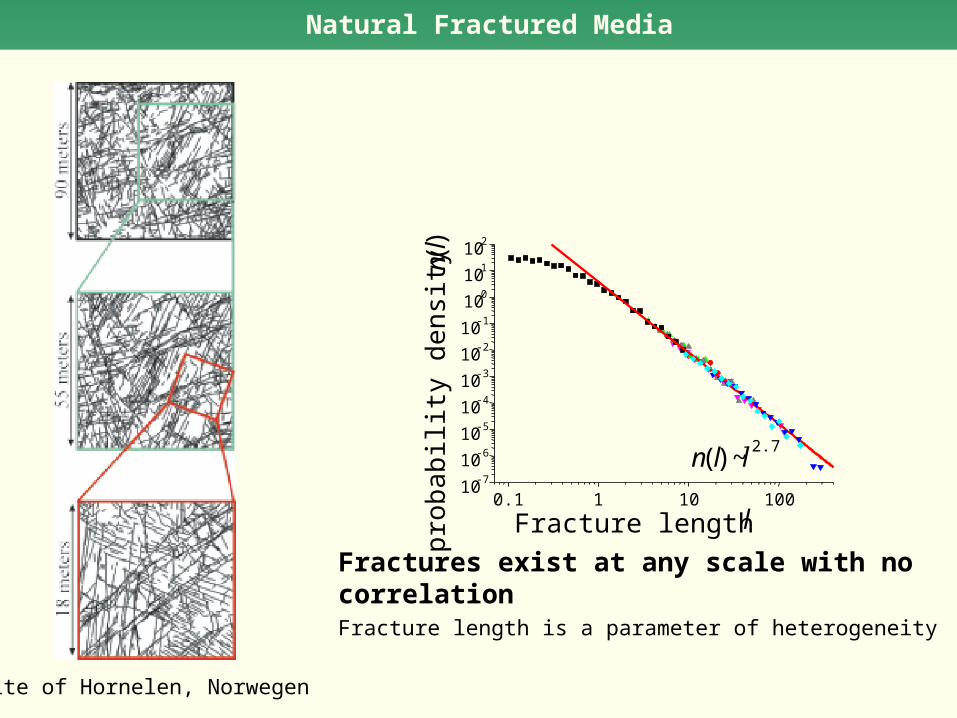
Natural Fractured Media

Fractures exist at any scale with no correlationFracture length is a parameter of heterogeneity

0.1 1 10 10010

-7

10-6

10-5

10-4

10-3

10-2

10-1

100

101

102

n(l)~l-2.7

prob

abili

ty d

ensi

ty

n(l)

Fracture length l

Site of Hornelen, Norwegen

Discrete Fracture Networks with impervious matrix

Stochastic computational domainlength distribution has a great impact : power law n(l) = l-a

3 types of networks based on the moments of length distribution

mean variation2 < a < 3

mean variation third moment3 < a < 4

mean variation third momenta > 4

Permeability field in porous media

Simple 2D or 3D geometrySimple 2D or 3D geometrystochastic permeability fieldstochastic permeability field

finitely or infinitely correlatedfinitely or infinitely correlated

MultifractalD2=1.7

finitely correlated medium

MultifractalD2=1.4

2( ) expY YY

C

rr

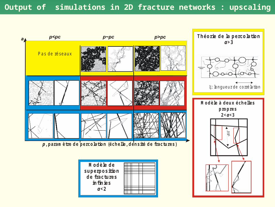
Output of simulations in 2D fracture networks : upscaling

Pas de réseaux

p , param ètre de percolation (échelle, densité de fractures)

Théorie de la percolation >3a

: longueur de corré lation

M odèle à deux échelles propres 2< <3a

M odèle de superposition de fractures

infinies <2a

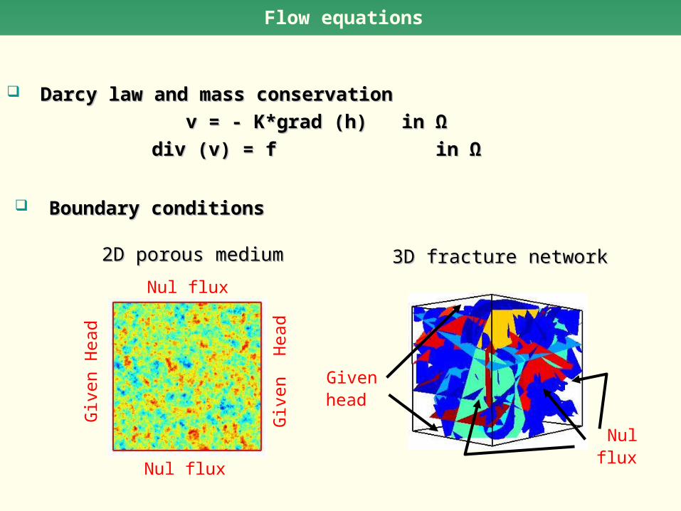
Darcy law and mass conservationDarcy law and mass conservation

v = - K*v = - K*grad (hgrad (h) in ) in ΩΩ

div (v) = f in div (v) = f in ΩΩ

BoundaryBoundary conditions conditions

Given head

Nul flux

3D fracture network3D fracture network

Giv

en

Head

Giv

en

H

ead

Nul flux

Nul flux

2D porous medium2D porous medium

Flow equations

Uncertainty Quantification methods

Probabilistic framework

Given statistics of the input data,

compute statistics of the random solution

stochastic permeability field K stochastic network Ω

stochastic flow equations

stochastic velocity field

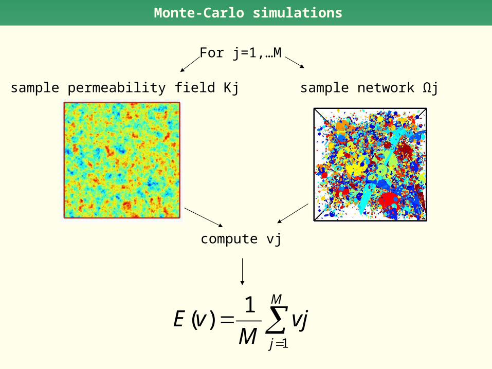
Monte-Carlo simulations

For j=1,…M

sample network Ωj

compute vj

M

j

vjM

vE1

1)(

sample permeability field Kj

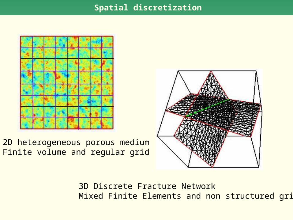
Spatial discretization

2D heterogeneous porous mediumFinite volume and regular grid

3D Discrete Fracture NetworkMixed Finite Elements and non structured grid

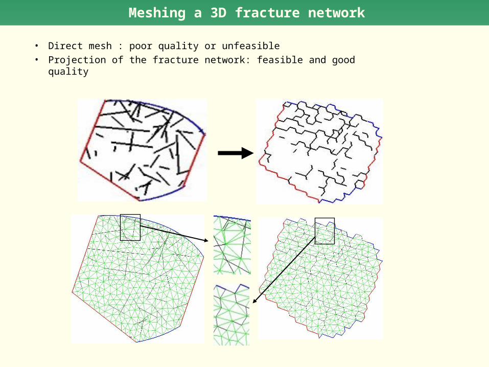
Meshing a 3D fracture network

• Direct mesh : poor quality or unfeasible

• Projection of the fracture network: feasible and good quality

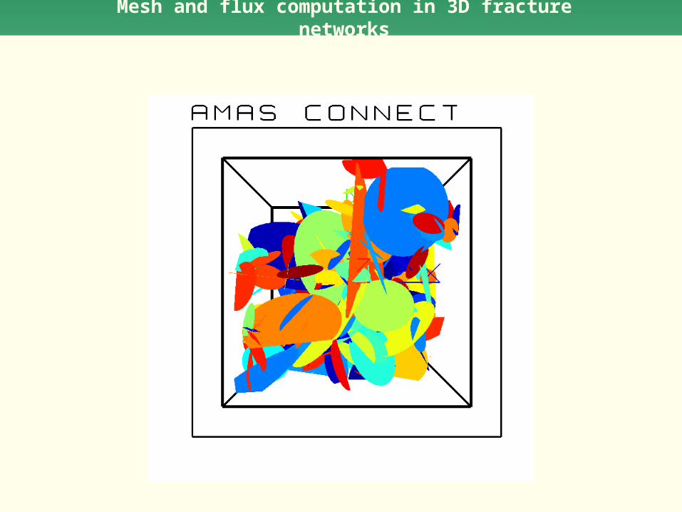
Mesh and flux computation in 3D fracture networks

Discrete flow numerical model

Linear system Ax=b

b: boundary conditions and source termA is a sparse matrix : NZ coefficientsMatrix-Vector product : O(NZ) opérationsDirect linear solvers: fill-in in Cholesy factor

Regular 2D mesh : N=n2 and NZ=5NRegular 3D mesh : N= n3 and NZ=7N

Fracture Network : N and NZ depend on the geometry

N = 8181

Intersections and 7 fractures

2D heterogeneous porous medium2D heterogeneous porous medium

memory size and CPU time with memory size and CPU time with PSPASESPSPASES

Theory : NZ(L) = O(N logN) Theory : Time = O(N1.5)

variance = 1, number of processors = 2

Sparse direct linear solvers

3D fracture network 3D fracture network

memory size and CPU time with PSPASESmemory size and CPU time with PSPASES

NZ(L) = O(N) ? Time = O(N) ?Theory to be done

Sparse direct linear solvers

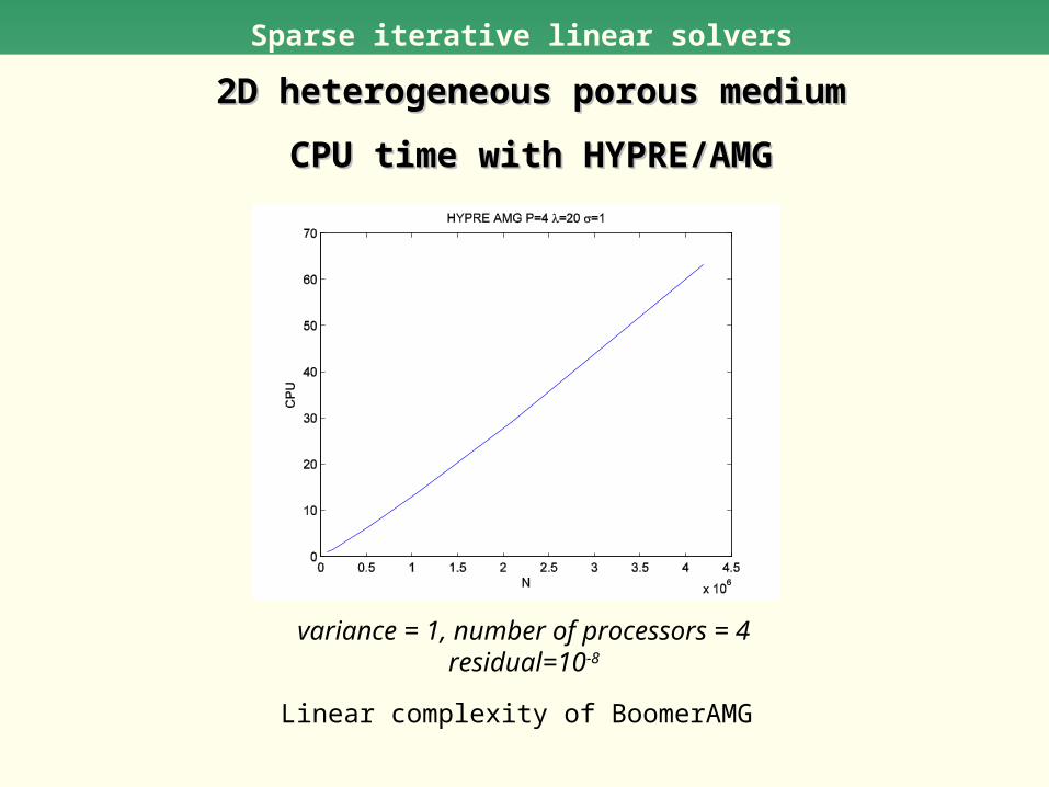
2D heterogeneous porous medium2D heterogeneous porous medium

CPU time with HYPRE/AMGCPU time with HYPRE/AMG

variance = 1, number of processors = 4residual=10-8

Linear complexity of BoomerAMG

Sparse iterative linear solvers

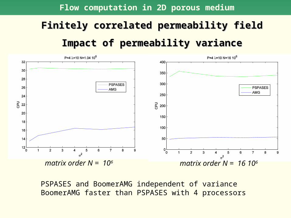
Flow computation in 2D porous medium

Finitely correlated permeability fieldFinitely correlated permeability field

Impact of permeability varianceImpact of permeability variance

matrix order N = 106

PSPASES and BoomerAMG independent of varianceBoomerAMG faster than PSPASES with 4 processors

matrix order N = 16 106

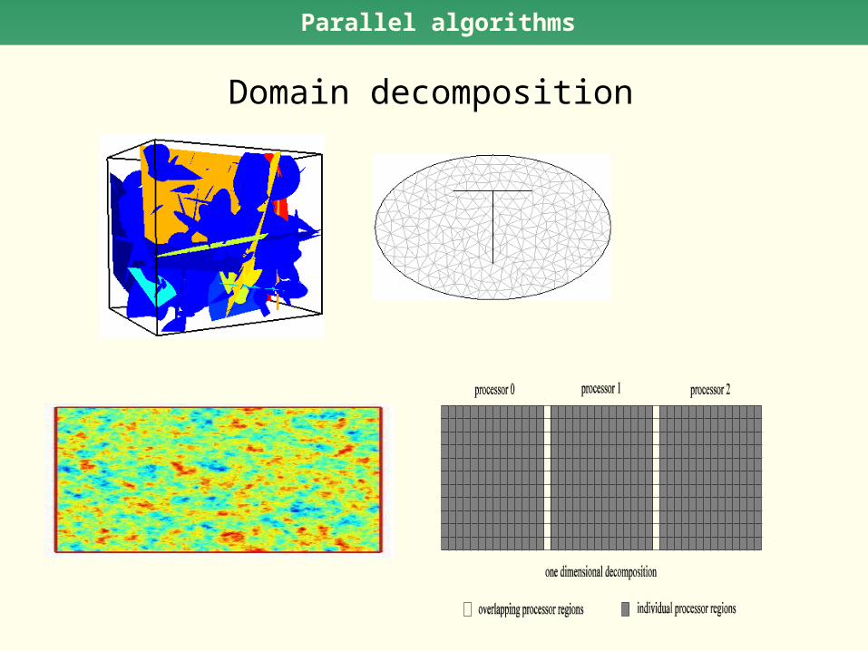
Parallel algorithms

Domain decomposition

parallel sparse linear solvers

2D heterogeneous porous medium2D heterogeneous porous medium

Direct and multigrid solversDirect and multigrid solvers

Parallel CPU timeParallel CPU time

variance = 9

matrix order N = 106 matrix order N = 4 106

Current work and perspectives

Current work• Iterative linear solvers for 3D fracture networks• 3D heterogeneous porous media• Subdomain method with Aitken-Schwarz acceleration• Transient flow in 2D and 3D porous media • Solute transport in 2D porous media • Grid computing and parametric simulations

Future work• Porous fractured media with rock • Well test interpretation• Site modeling• UQ methods