high-order time-adaptive numerical methods for the allen
TRANSCRIPT

High-Order Time-AdaptiveNumerical Methods For The
Allen-Cahn and Cahn-HilliardEquations
by
Mark Ryerson Willoughby
B.Sc., Brock University, 2009
A THESIS SUBMITTED IN PARTIAL FULFILLMENT OFTHE REQUIREMENTS FOR THE DEGREE OF
MASTER OF SCIENCE
in
The Faculty of Graduate Studies
(Mathematics)
THE UNIVERSITY OF BRITISH COLUMBIA
(Vancouver)
December 2011
c© Mark Ryerson Willoughby 2011

Abstract
In some nonlinear reaction-diffusion equations of interest in applications,
there are transition layers in solutions that separate two or more materials
or phases in a medium when the reaction term is very large. Two well known
equations that are of this type: The Allen-Cahn equation and the Cahn-
Hillard equation. The transition layers between phases evolve over time and
can move very slowly. The models have an order parameter ε. Fully devel-
oped transition layers have a width that scales linearly with ε. As ε→ 0, the
time scale of evolution can also change and the problem becomes numerically
challenging.
We consider several numerical methods to obtain solutions to these equa-
tions, in order to build a robust, efficient and accurate numerical strategy.
Explicit time stepping methods have severe time step constraints, so we di-
rect our attention to implicit schemes. Second and third order time-adaptive
methods are presented using spectral discretization in space. The implicit
problem is solved using the conjugate gradient method with a novel pre-
conditioner. The behaviour of the preconditioner is investigated, and the
ii
Abstract
dependence on ε and time step size is identified.
The Allen-Cahn and Cahn-Hilliard equations have been used extensively to
model phenomena in materials science. We strongly believe that our high-
order adaptive approach is also easily extensible to higher order models with
application to pore formation in functionalized polymers and to cancerous
tumor growth simulation. This is the subject of ongoing research.
iii
Table of Contents
Abstract . . . . . . . . . . . . . . . . . . . . . . . . . . . . . . . . . . ii
Table of Contents . . . . . . . . . . . . . . . . . . . . . . . . . . . . iv
List of Tables . . . . . . . . . . . . . . . . . . . . . . . . . . . . . . vii
List of Figures . . . . . . . . . . . . . . . . . . . . . . . . . . . . . . ix
Acknowledgements . . . . . . . . . . . . . . . . . . . . . . . . . . . xiii
1 Introduction . . . . . . . . . . . . . . . . . . . . . . . . . . . . . 1
2 Analytical Methods . . . . . . . . . . . . . . . . . . . . . . . . . 10
3 Basic Numerical Methods . . . . . . . . . . . . . . . . . . . . . 16
3.1 Forward Euler Method . . . . . . . . . . . . . . . . . . . . . . 18
3.2 Backward Euler Method . . . . . . . . . . . . . . . . . . . . . 20
3.3 Finite Differences for Spatial Derivatives . . . . . . . . . . . . 21
3.4 Discretization . . . . . . . . . . . . . . . . . . . . . . . . . . . 23
3.5 Newton Iteration . . . . . . . . . . . . . . . . . . . . . . . . . 25
iv
Table of Contents
3.6 Backward Euler Solution . . . . . . . . . . . . . . . . . . . . 27
3.7 Convergence . . . . . . . . . . . . . . . . . . . . . . . . . . . 28
3.8 Adaptive Time Stepping . . . . . . . . . . . . . . . . . . . . . 30
3.9 Local Error Method . . . . . . . . . . . . . . . . . . . . . . . 31
3.10 Ripening Time . . . . . . . . . . . . . . . . . . . . . . . . . . 36
3.11 Numerical Experiment - Allen-Cahn . . . . . . . . . . . . . . 37
3.11.1 Comparison to Uniform Method . . . . . . . . . . . . 40
3.12 Numerical Experiment - Cahn-Hilliard . . . . . . . . . . . . . 41
4 Solution Techniques . . . . . . . . . . . . . . . . . . . . . . . . 46
4.1 Conjugate Gradient . . . . . . . . . . . . . . . . . . . . . . . 46
4.2 Preconditioning . . . . . . . . . . . . . . . . . . . . . . . . . . 49
5 Spectral Methods in Space . . . . . . . . . . . . . . . . . . . . 55
5.1 Using the Fast Fourier Transform . . . . . . . . . . . . . . . . 62
6 High-Order Time step Techniques . . . . . . . . . . . . . . . 64
6.1 Runge Kutta Methods . . . . . . . . . . . . . . . . . . . . . . 64
6.1.1 Singly Diagonal Implicit Runge Kutta 2 (SDIRK2) . . 67
6.1.2 Singly Diagonal Implicit Runge Kutta 3 (SDIRK3) . . 69
6.2 Linear Multi Step Methods . . . . . . . . . . . . . . . . . . . 71
6.2.1 Adams-Bashforth 2 (AB2) . . . . . . . . . . . . . . . . 71
6.2.2 Adams-Bashforth 3 (AB3) . . . . . . . . . . . . . . . . 73
6.2.3 Backward Difference Formula 2 (BDF2) . . . . . . . . 74
v
Table of Contents
6.2.4 Backward Difference Formula 3 (BDF3) . . . . . . . . 76
6.3 BDF2 with AB2 Local Error Estimation and SDIRK2 Restart 76
6.3.1 Ripening Time . . . . . . . . . . . . . . . . . . . . . . 80
6.4 BDF3 with AB3 Local Error Estimation and SDIRK3 Restart 82
6.4.1 Ripening Time . . . . . . . . . . . . . . . . . . . . . . 83
7 Numerical Experiments . . . . . . . . . . . . . . . . . . . . . . 86
7.1 Allen-Cahn in 1D . . . . . . . . . . . . . . . . . . . . . . . . 87
7.2 Cahn-Hilliard in 1D . . . . . . . . . . . . . . . . . . . . . . . 91
7.3 Allen-Cahn in 2D . . . . . . . . . . . . . . . . . . . . . . . . 95
7.4 Cahn-Hilliard in 2D . . . . . . . . . . . . . . . . . . . . . . . 99
8 Conclusions and Future Work . . . . . . . . . . . . . . . . . . 104
8.1 Future Work . . . . . . . . . . . . . . . . . . . . . . . . . . . 106
Bibliography . . . . . . . . . . . . . . . . . . . . . . . . . . . . . . . 109
vi
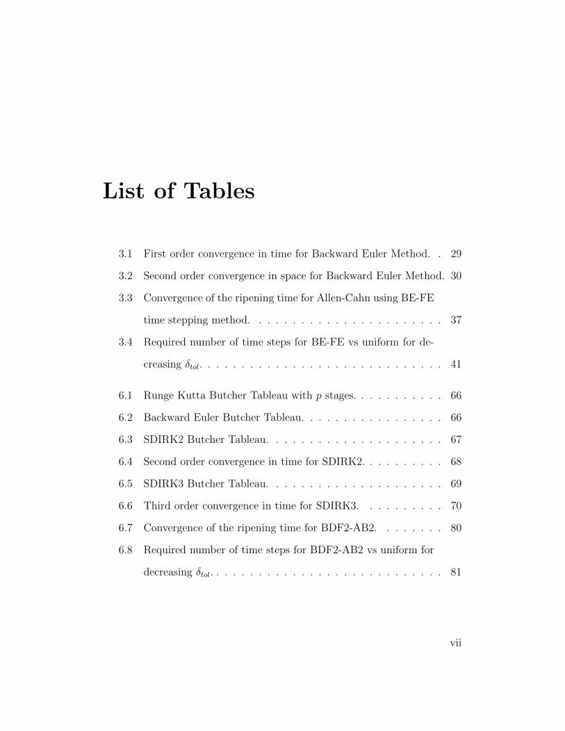
List of Tables
3.1 First order convergence in time for Backward Euler Method. . 29
3.2 Second order convergence in space for Backward Euler Method. 30
3.3 Convergence of the ripening time for Allen-Cahn using BE-FE
time stepping method. . . . . . . . . . . . . . . . . . . . . . . 37
3.4 Required number of time steps for BE-FE vs uniform for de-
creasing δtol. . . . . . . . . . . . . . . . . . . . . . . . . . . . . 41
6.1 Runge Kutta Butcher Tableau with p stages. . . . . . . . . . . 66
6.2 Backward Euler Butcher Tableau. . . . . . . . . . . . . . . . . 66
6.3 SDIRK2 Butcher Tableau. . . . . . . . . . . . . . . . . . . . . 67
6.4 Second order convergence in time for SDIRK2. . . . . . . . . . 68
6.5 SDIRK3 Butcher Tableau. . . . . . . . . . . . . . . . . . . . . 69
6.6 Third order convergence in time for SDIRK3. . . . . . . . . . 70
6.7 Convergence of the ripening time for BDF2-AB2. . . . . . . . 80
6.8 Required number of time steps for BDF2-AB2 vs uniform for
decreasing δtol. . . . . . . . . . . . . . . . . . . . . . . . . . . . 81
vii
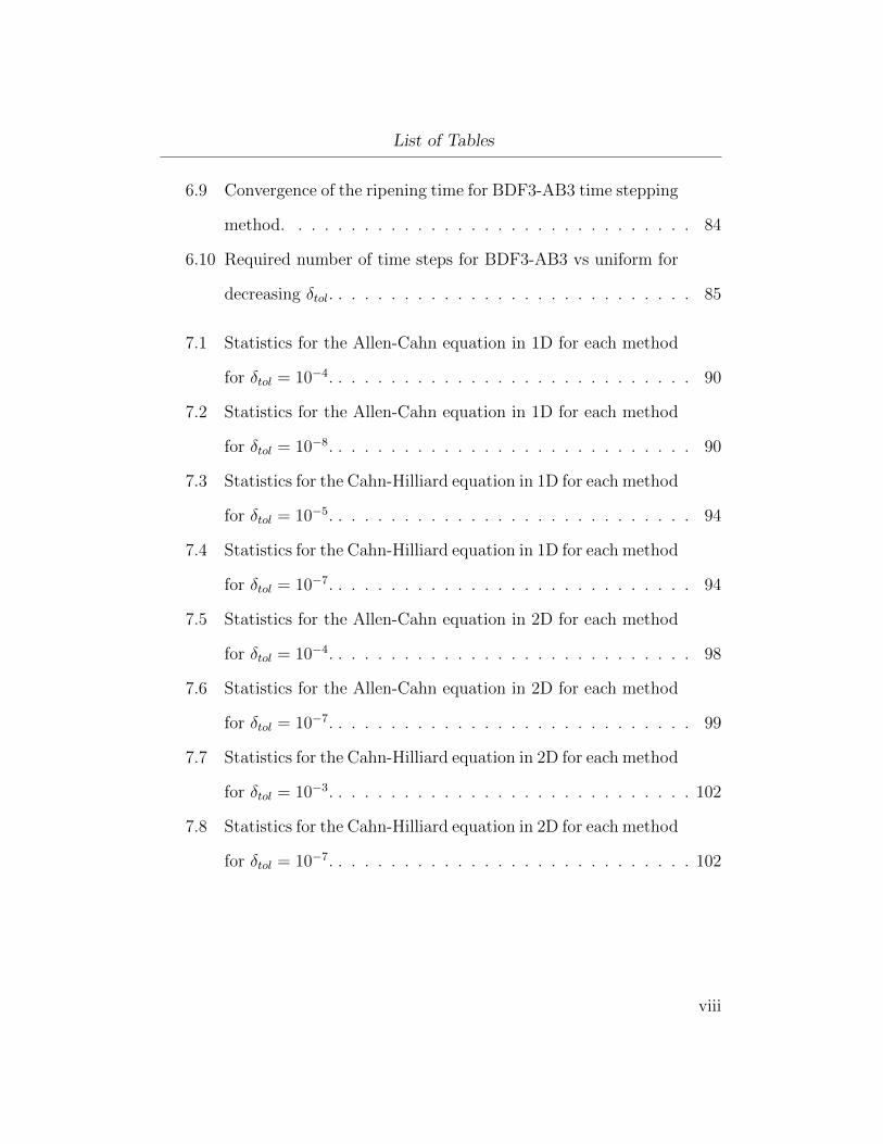
List of Tables
6.9 Convergence of the ripening time for BDF3-AB3 time stepping
method. . . . . . . . . . . . . . . . . . . . . . . . . . . . . . . 84
6.10 Required number of time steps for BDF3-AB3 vs uniform for
decreasing δtol. . . . . . . . . . . . . . . . . . . . . . . . . . . . 85
7.1 Statistics for the Allen-Cahn equation in 1D for each method
for δtol = 10−4. . . . . . . . . . . . . . . . . . . . . . . . . . . . 90
7.2 Statistics for the Allen-Cahn equation in 1D for each method
for δtol = 10−8. . . . . . . . . . . . . . . . . . . . . . . . . . . . 90
7.3 Statistics for the Cahn-Hilliard equation in 1D for each method
for δtol = 10−5. . . . . . . . . . . . . . . . . . . . . . . . . . . . 94
7.4 Statistics for the Cahn-Hilliard equation in 1D for each method
for δtol = 10−7. . . . . . . . . . . . . . . . . . . . . . . . . . . . 94
7.5 Statistics for the Allen-Cahn equation in 2D for each method
for δtol = 10−4. . . . . . . . . . . . . . . . . . . . . . . . . . . . 98
7.6 Statistics for the Allen-Cahn equation in 2D for each method
for δtol = 10−7. . . . . . . . . . . . . . . . . . . . . . . . . . . . 99
7.7 Statistics for the Cahn-Hilliard equation in 2D for each method
for δtol = 10−3. . . . . . . . . . . . . . . . . . . . . . . . . . . . 102
7.8 Statistics for the Cahn-Hilliard equation in 2D for each method
for δtol = 10−7. . . . . . . . . . . . . . . . . . . . . . . . . . . . 102
viii

List of Figures
1.1 Three EBSD maps of the stored energy in an Al-Mg-Mn al-
loy after exposure to increasing recrystallization temperature.
The volume fraction of recrystallized grains (light) increases
with temperature for a given time. Source: Manchester Uni-
versity (2003) . . . . . . . . . . . . . . . . . . . . . . . . . . . 3
1.2 Recrystallization of a metallic material (a → b) and crystal
grains growth (b → c → d). Source: Wikipedia Commons. . . 3
2.1 Possible initial conditions with transition layers between u = ±1. 11
2.2 (a). Matching requirement for u = −1 and u = +1 at x = x0.
(b). Numerical solution showing transition layer near x = x0. . 12
2.3 Transition layer solution to match stable solutions u = ±1. . . 15
3.1 Graphical interpretation for Newton Iteration. . . . . . . . . . 25
3.2 Backward Euler Solution with γ = 2 vs. γ = 4 in 1D. . . . . . 34
3.3 Number of changes of time step with the time steps required
with varying γ in the BE-FE solution. . . . . . . . . . . . . . 35
ix
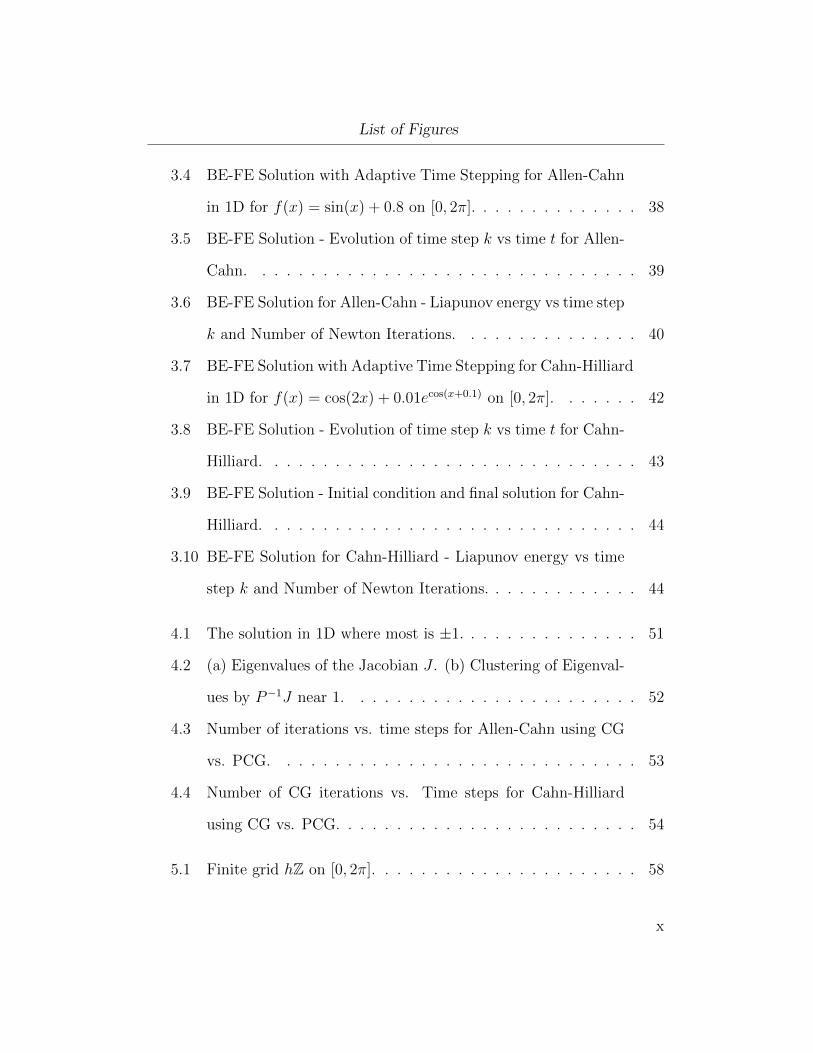
List of Figures
3.4 BE-FE Solution with Adaptive Time Stepping for Allen-Cahn
in 1D for f(x) = sin(x) + 0.8 on [0, 2π]. . . . . . . . . . . . . . 38
3.5 BE-FE Solution - Evolution of time step k vs time t for Allen-
Cahn. . . . . . . . . . . . . . . . . . . . . . . . . . . . . . . . 39
3.6 BE-FE Solution for Allen-Cahn - Liapunov energy vs time step
k and Number of Newton Iterations. . . . . . . . . . . . . . . 40
3.7 BE-FE Solution with Adaptive Time Stepping for Cahn-Hilliard
in 1D for f(x) = cos(2x) + 0.01ecos(x+0.1) on [0, 2π]. . . . . . . 42
3.8 BE-FE Solution - Evolution of time step k vs time t for Cahn-
Hilliard. . . . . . . . . . . . . . . . . . . . . . . . . . . . . . . 43
3.9 BE-FE Solution - Initial condition and final solution for Cahn-
Hilliard. . . . . . . . . . . . . . . . . . . . . . . . . . . . . . . 44
3.10 BE-FE Solution for Cahn-Hilliard - Liapunov energy vs time
step k and Number of Newton Iterations. . . . . . . . . . . . . 44
4.1 The solution in 1D where most is ±1. . . . . . . . . . . . . . . 51
4.2 (a) Eigenvalues of the Jacobian J . (b) Clustering of Eigenval-
ues by P−1J near 1. . . . . . . . . . . . . . . . . . . . . . . . 52
4.3 Number of iterations vs. time steps for Allen-Cahn using CG
vs. PCG. . . . . . . . . . . . . . . . . . . . . . . . . . . . . . 53
4.4 Number of CG iterations vs. Time steps for Cahn-Hilliard
using CG vs. PCG. . . . . . . . . . . . . . . . . . . . . . . . . 54
5.1 Finite grid hZ on [0, 2π]. . . . . . . . . . . . . . . . . . . . . . 58
x
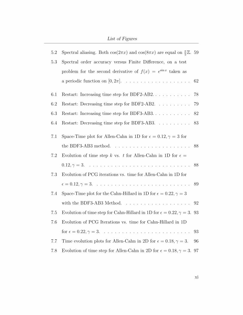
List of Figures
5.2 Spectral aliasing. Both cos(2πx) and cos(8πx) are equal on π5Z. 59
5.3 Spectral order accuracy versus Finite Difference, on a test
problem for the second derivative of f(x) = esinx taken as
a periodic function on [0, 2π]. . . . . . . . . . . . . . . . . . . 62
6.1 Restart: Increasing time step for BDF2-AB2. . . . . . . . . . . 78
6.2 Restart: Decreasing time step for BDF2-AB2. . . . . . . . . . 79
6.3 Restart: Increasing time step for BDF3-AB3. . . . . . . . . . . 82
6.4 Restart: Decreasing time step for BDF3-AB3. . . . . . . . . . 83
7.1 Space-Time plot for Allen-Cahn in 1D for ε = 0.12, γ = 3 for
the BDF3-AB3 method. . . . . . . . . . . . . . . . . . . . . . 88
7.2 Evolution of time step k vs. t for Allen-Cahn in 1D for ε =
0.12, γ = 3. . . . . . . . . . . . . . . . . . . . . . . . . . . . . 88
7.3 Evolution of PCG iterations vs. time for Allen-Cahn in 1D for
ε = 0.12, γ = 3. . . . . . . . . . . . . . . . . . . . . . . . . . . 89
7.4 Space-Time plot for the Cahn-Hillard in 1D for ε = 0.22, γ = 3
with the BDF3-AB3 Method. . . . . . . . . . . . . . . . . . . 92
7.5 Evolution of time step for Cahn-Hillard in 1D for ε = 0.22, γ = 3. 93
7.6 Evolution of PCG Iterations vs. time for Cahn-Hillard in 1D
for ε = 0.22, γ = 3. . . . . . . . . . . . . . . . . . . . . . . . . 93
7.7 Time evolution plots for Allen-Cahn in 2D for ε = 0.18, γ = 3. 96
7.8 Evolution of time step for Allen-Cahn in 2D for ε = 0.18, γ = 3. 97
xi
List of Figures
7.9 Evolution of PCG iterations vs. time for Allen-Cahn in 2D for
ε = 0.18, γ = 3. . . . . . . . . . . . . . . . . . . . . . . . . . . 98
7.10 Time evolution plots for Cahn-Hilliard in 2D for ε = 0.18, γ = 2.100
7.11 Evolution of time step for Cahn-Hilliard in 2D for ε = 0.18, γ =
2. . . . . . . . . . . . . . . . . . . . . . . . . . . . . . . . . . . 101
7.12 Evolution of PCG iterations vs. time for Cahn-Hilliard in 2D
for ε = 0.18, γ = 2. . . . . . . . . . . . . . . . . . . . . . . . . 101
8.1 Composite grid used in adaptive-in-space methods. . . . . . . 107
xii

Acknowledgements
I would like to thank my supervisor Dr. Brian Wetton. His help throughout
this project has been invaluable, and I appreciate his patience and many
observations and directions throughout our meetings. It continues to be an
honour to work with Brian and our research group. I also would like to thank
Lee Yupitun, the math graduate secretary, for all her administrative help.
I would also like to thank Dr. Scott MacLachlan. His contribution of a
linear model preconditioner is the highlight and main contribution of this
thesis.
My research colleagues, Iain Moyles, Michael Lindstrom, Kai Rothauge and
Ricardo Alves-Martins have also been valuable editors and contributors, and
they offer discussion as well as support and friendship. I have watched the
development of our research group since I have been involved and I am proud
to be in company of such extraordinary people.
My family also has been a pillar of support throughout this project. I want
xiii

Acknowledgements
to thank my mother and sister for always being there for me. I also want
to thank my father. While you may not be here with me now, I am here
because of you.
xiv
Chapter 1
Introduction
Reaction-diffusion equations are one of the most significant tools in material
sciences modelling. When the overall effect of reaction kinetics is larger than
diffusion, transition layers form which physically represent a separation of
two unique states or phases. Phase separation of metals in alloys as well
as crystal grains in a metal that grow in competition with each other dur-
ing annealing are examples of this transition layer behaviour. Two common
equations that model the reaction kinetics in reaction-diffusion systems in
material science, as well as diffusion-convection models in fluid dynamics are
the Allen-Cahn and Cahn-Hilliard equations.
The Allen-Cahn equation was first introduced and named after Allen and
Cahn in 1979 [1], and the Cahn-Hilliard by Cahn and Hilliard in 1958 [2].
Discretization and specific solutions to both equations have been studied ex-
tensively, see [3, 4, 5, 6, 7]. Analytical methods such as asymptotic analysis
will not yield the full dynamics of the solution in general. Therefore an ef-
ficient and robust numerical strategy is needed to adequately describe the
solution. We expect that the solution will admit transition layers. However,
1
Chapter 1. Introduction
these layers are not static which means that care will have to be given in
the time stepping procedure. Numerical methods for time stepping that are
explicit will encounter severe time step constraints for stability, thus we seek
implicit schemes. We will consider second and third order time-adaptive
methods using spectral discretization in space. Using a novel preconditioner,
the implicit problem is solved using the conjugate gradient method. This
thesis will investigate these numerical schemes.
Consider annealing, the process by which metal, glass etc. is heated and
allowed to cool slowly. In the context of metal, this will harden or strengthen
the metal, relieve stresses and improve the structure and ductility. Common
examples in practice are the metals: copper, steel, silver and brass. The
metal is heated above the recrystallization temperature and kept at that
temperature for a length of time. Diffusion of the atoms inside the metal will
achieve an equilibrium state. Three stages of annealing consist of recovery,
recrystallization and equilibrium. The first stage results in softening of the
metal through removal of crystal defects. The second stage exhibits grains
that nucleate and grow to replace those deformed by internal stresses. The
third stage is the state by which this growth has reached equilibrium [8]. Re-
crystallization is the process that can be modelled with the Allen-Cahn and
Cahn-Hilliard models; deformed grains are replaced by undeformed grains
that nucleate and grow until the original grains have been entirely consumed.
Consider the Aluminum-Magnesium-Manganese alloy shown in Figure 1.1.
2
Chapter 1. Introduction
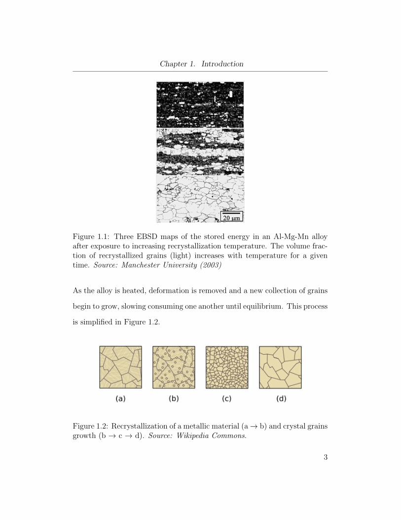
Figure 1.1: Three EBSD maps of the stored energy in an Al-Mg-Mn alloyafter exposure to increasing recrystallization temperature. The volume frac-tion of recrystallized grains (light) increases with temperature for a giventime. Source: Manchester University (2003)
As the alloy is heated, deformation is removed and a new collection of grains
begin to grow, slowing consuming one another until equilibrium. This process
is simplified in Figure 1.2.
Figure 1.2: Recrystallization of a metallic material (a→ b) and crystal grainsgrowth (b → c → d). Source: Wikipedia Commons.
3

Chapter 1. Introduction
As stated, the behaviour of annealing, and many other problems, can be mod-
elled using the Allen-Cahn equation, which is a partial differential equation
having the general form
ut = ε2∆u− f(u), x ∈ Ω, ε 1, (1.1)
u(x, 0) = u0(x),
where we have variables t for time and x for position, f(u) is nonlinear, and
with boundary conditions dependent on the problem for a domain Ω. The
variable u can be considered the concentration, volume difference or phase
state between materials. The small parameter ε > 0 is known as the inter-
action length, and also describes the thickness of the transition boundary
between materials, also called the transition layer. We assume that ε is small
with respect to the length scale of the domain of the problem. This captures
the dominating effect of the reaction kinetics and appears in the equation to
represent an effective diffusivity.
Like most material science applications, we can assume a certain periodicity
in the lattice structure and so we will impose periodic boundary conditions
to mimic a large system [9]. The rationale is that a small square section of
the metal can be repeated to simulate the entire plate. With this being said,
we consider our domain, Ω = [0, 2π]d where d is the dimension of the prob-
lem. We have chosen this domain due to our application of spectral methods
4

Chapter 1. Introduction
which we will investigate in chapter 5. The initial value problems that we
will then consider in this thesis are the Allen-Cahn equation
ut = ε2∆u− w′(u), x ∈ [0, 2π]d, ε 1,
Periodic Boundary Conditions,
u(x, 0) = u0(x),
w(u) = 14(1− u2)2,
(1.2)
where our nonlinear term f(u) = w′(u). The term w(u) is known as the
Ginzburg-Landau double well potential. We also consider the Cahn Hilliard
problem
ut = −∆ [ε2∆u− w′(u)] , x ∈ [0, 2π]d, ε 1,
Periodic Boundary Conditions,
u(x, 0) = u0(x),
w(u) = 14(1− u2)2,
(1.3)
which is fourth order in space. Equations (1.2) and (1.3) both have solutions
that describe the separation of the medium we desire to model, where there is
an abrupt change from one phase u = 1 to the other u = −1, the transition
layers, such as we see in Figure 1.1. The transition layers between these
phases will move slowly over time for the problems we are considering. As
such, we are interested in the behaviour of long time scales when ε → 0.
An important feature of the Allen-Cahn and Cahn-Hilliard equations is that
5
Chapter 1. Introduction
they can be viewed as the gradient flow of the Liapunov energy functional
E(u) =
∫Ω
(ε2
2|∇u|2 + w(u)
)dx, (1.4)
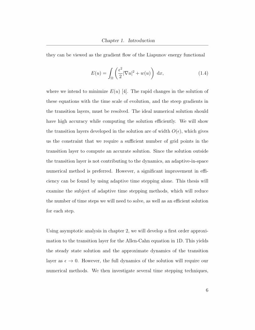
where we intend to minimize E(u) [4]. The rapid changes in the solution of
these equations with the time scale of evolution, and the steep gradients in
the transition layers, must be resolved. The ideal numerical solution should
have high accuracy while computing the solution efficiently. We will show
the transition layers developed in the solution are of width O(ε), which gives
us the constraint that we require a sufficient number of grid points in the
transition layer to compute an accurate solution. Since the solution outside
the transition layer is not contributing to the dynamics, an adaptive-in-space
numerical method is preferred. However, a significant improvement in effi-
ciency can be found by using adaptive time stepping alone. This thesis will
examine the subject of adaptive time stepping methods, which will reduce
the number of time steps we will need to solve, as well as an efficient solution
for each step.
Using asymptotic analysis in chapter 2, we will develop a first order approxi-
mation to the transition layer for the Allen-Cahn equation in 1D. This yields
the steady state solution and the approximate dynamics of the transition
layer as ε → 0. However, the full dynamics of the solution will require our
numerical methods. We then investigate several time stepping techniques,
6
Chapter 1. Introduction
starting with a first order method in chapter 3 using our most basic methods.
The simplest method to implement is Backward Euler. For small ε, we will
show that an approximation using uniform time steps cannot compute the
solution to its steady state in a reasonable time, and adaptivity in time is
essential. We will compute the solution using Forward Euler as a predictor,
and show that the difference between these solutions will estimate the local
error, which then can be used to decide if we increase or decrease the time
step. We will see the solution quickly reaches a metastable state, where the
transition layer has formed and now moves slowly.
To solve the nonlinear system of equations for each time step, we use Newton
Iteration. In chapter 4 we develop a Conjugate Gradient method to solve for
each iteration, where a linear system must be solved. We then develop a
Preconditioned Conjugate Gradient method for this linear problem with a
novel preconditioner that is a constant coefficient version of the system at
the pure phase states u = ±1, suggested to us by Scott MacLachlan of Tufts
University [11]. The width of the transition layers in our problem are much
smaller than the entire domain for small ε. The dynamics of the solution
do not change outside of the layer, thus a linear model would be a good
candidate as a preconditioner. We will show that indeed a linear model will
improve each CG solve for our methods. The development and investigation
of this solver is the main contribution of this thesis.
7
Chapter 1. Introduction
It is our goal to show that adaptivity in time is sufficient for an efficient
numerical method. This is achieved by using spectral methods in space.
In chapter 5, we develop a Fourier periodic spectral method. As a result, at
each time step we will require a solution to a more dense system of discretized
equations. However, since this system is composed of N Fourier basis func-
tions, a sufficient N will introduce almost no spatial error as a result [12].
We can approximate the solution with a minimum number of basis functions
growing linearly with 1/ε. We will show that spectral methods give a good
efficient solution to our problem.
We then consider higher order time stepping methods to compare to our
first order method. In chapter 6, we will look at second and third order
singly-diagonal implicit Runge Kutta methods as well as linear multi step
methods to obtain second and third order adaptive-in-time methods. Each
adaptive time stepping method derives its adaptivity from the local error
estimator. There are several estimators that can be used, but an efficient
estimator will be a explicit method which is quick to calculate and is of the
same order of the method. We have chosen the explicit Adams-Bashforth
method for this purpose. At each time step, we then calculate a pair of so-
lutions, implicit and explicit, and use the maximum norm of the difference
as our local error estimator.
In chapter 7 several full numerical simulations will be presented for both
8

Chapter 1. Introduction
Allen-Cahn and Cahn-Hilliard in 1D and 2D for small ε. The programming
for each method will be done in MATLAB and detailed comparison will be
used to determine the advantages and disadvantages of each method. We
will show that our second and third order methods are more efficient than
the simple Backward Euler method.
Phenomena in material science have often been modelled using the Allen-
Cahn and Cahn-Hilliard equations. We strongly believe that the methods
proposed in this thesis will be easily extensible to higher order models and
applications, such as pore formation in functionalized polymers or Polymer
Electrolyte Membranes (PEM) of fuel cells [14], or to cancerous tumor growth
simulation (using a sixth order Cahn-Hilliard equation) used in cancer re-
search [15].
9

Chapter 2
Analytical Methods
Considerable work has been done using analytical methods to understand the
behaviour of solutions to the Allen-Cahn and Cahn-Hilliard equations, see [5,
16, 17, 18, 19]. While explicit analytic solutions cannot be found in general,
we can use analytical techniques to gain insight into the dynamics. One such
way to explore dynamics is to look for steady state solutions through the use
of asymptotic analysis. Consider the Allen-Cahn equation in one dimension
(1D)
ut = ε2uxx + u− u3. (2.1)
Consider situations when the diffusion is negligible because ε 1. This oc-
curs in regions where the composition consists almost entirely of one material.
The boundary between materials will be the region of interest for diffusion.
Neglecting diffusion in (2.1) leads to ut = u − u3, which is an ordinary dif-
ferential equation (ODE) which has steady state solutions of u∗ = 0,±1. We
can perform a linear stability analysis in the absence of diffusion of the form
u = u∗+φeλt for eigenvalues λ. We conclude that the eigenvalues for u∗ = ±1
10
Chapter 2. Analytical Methods
are negative while the eigenvalue for u∗ = 0 is positive. Consequently, the
states u∗ = ±1 are stable while the state u∗ = 0 is unstable.
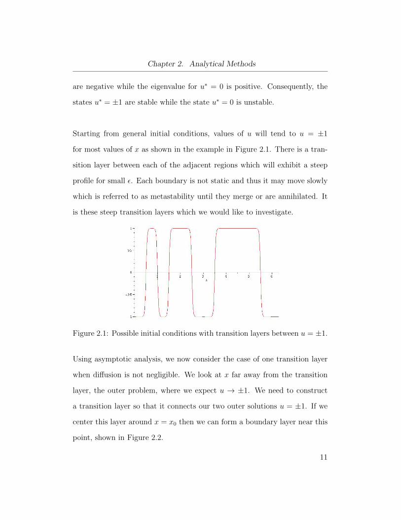
Starting from general initial conditions, values of u will tend to u = ±1
for most values of x as shown in the example in Figure 2.1. There is a tran-
sition layer between each of the adjacent regions which will exhibit a steep
profile for small ε. Each boundary is not static and thus it may move slowly
which is referred to as metastability until they merge or are annihilated. It
is these steep transition layers which we would like to investigate.
Figure 2.1: Possible initial conditions with transition layers between u = ±1.
Using asymptotic analysis, we now consider the case of one transition layer
when diffusion is not negligible. We look at x far away from the transition
layer, the outer problem, where we expect u → ±1. We need to construct
a transition layer so that it connects our two outer solutions u = ±1. If we
center this layer around x = x0 then we can form a boundary layer near this
point, shown in Figure 2.2.
11

Chapter 2. Analytical Methods
Figure 2.2: (a). Matching requirement for u = −1 and u = +1 at x = x0.(b). Numerical solution showing transition layer near x = x0.
Focusing on the small region between the outer solution u = ±1, we can
define an inner region variable, y = x−x0ε
, −∞ < y < ∞ so that the inner
problem becomes
ut = uyy + u− u3. (2.2)
The scaling on y is chosen so that diffusion is not negligible. The power of ε
that appears in y indicates that the transition layer has a width of O(ε). We
can look for steady state solutions of (2.2) by looking at the problem
uyy = u3 − u.
12

Chapter 2. Analytical Methods
Multiplying by uy on both sides gives
uyuyy = uyu3 − uyu
1
2(u2
y)y =1
4(u4)y −
1
2(u2)y.
Integrating both sides with respect to y yields
∫(u2
y)y dx =1
2
∫(u4)y dx−
∫(u2)y dx
u2y =
1
2u4 − u2 + C,
where C is an arbitrary constant. To determine the constant C we consider
the boundary conditions uy → 0 and u → ±1 when y → ±∞ which corre-
sponds to the appropriate matching conditions with x− x0, which is O(1) in
the outer solution. We have
C = u2 − 1
2u4
∣∣∣∣u=±1
=1
2
Then our problem for uy is now
uy = ±√
1
2u4 − u2 +
1
2
= ± 1√2
√(u2 − 1)2
= ± 1√2
(u2 − 1).
13
Chapter 2. Analytical Methods
Since we have chosen our matching condition to go from u = −1 to u = +1
we take the negative square root. Separating variables and integrating, we
have
∫1
u2 − 1du = − 1√
2y +D.
Upon performing the integration we get
−arctanh(u) = − 1√2y +D
u = tanh
(y√2
+D
).
Returning to the outer variable x, we have
u = tanh
(x− x0√
2ε+D
).
The constant D in this case is due to the translational invariance of this
function on an infinite domain. Since we chose to center the transition layer
at x = x0 then we are imposing that u = 0 there. This then determines that
the constant D must be zero. Therefore, the solution to the transition layer
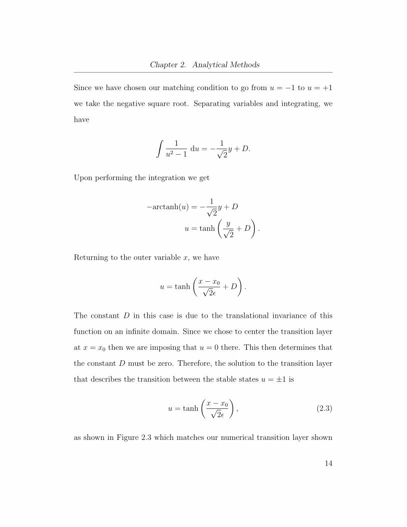
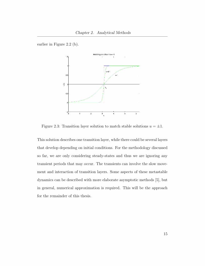
that describes the transition between the stable states u = ±1 is
u = tanh
(x− x0√
2ε
), (2.3)
as shown in Figure 2.3 which matches our numerical transition layer shown
14
Chapter 2. Analytical Methods
earlier in Figure 2.2 (b).
Figure 2.3: Transition layer solution to match stable solutions u = ±1.
This solution describes one transition layer, while there could be several layers
that develop depending on initial conditions. For the methodology discussed
so far, we are only considering steady-states and thus we are ignoring any
transient periods that may occur. The transients can involve the slow move-
ment and interaction of transition layers. Some aspects of these metastable
dynamics can be described with more elaborate asymptotic methods [5], but
in general, numerical approximation is required. This will be the approach
for the remainder of this thesis.
15

Chapter 3
Basic Numerical Methods
Due to the complexity associated with many partial differential equations,
analytical techniques are often unable to provide us with explicit solutions.
Though there are many approaches to obtain insight into a partial differ-
ential equation (PDE), it is our goal to obtain an accurate solution using
a numerical method. To do this, we restrict the domain of the problem to
only a finite number of points (xi, tn), i = 0, 1, ..., I, n = 0, 1, ..., N , called the
computational domain. The scope of this thesis will be a periodic domain
[0, 2π]d, where d is the dimension of the problem. At each of the finite points
x0, x1, ..., xI , which we call a mesh, we numerically evaluate a solution u to
the PDE for a time interval [0, T ]. We first consider how the time derivative
is computed in the context of a numerical scheme. By partitioning the given
time interval [0, T ] into N subintervals t0, t1, ..., tN , and time step k, we can
compute a numerical approximation to the time derivative. If we consider a
uniform time step k = tn+1 − tn, then we would call this a regular interval.
Consider first the scalar initial value problem
du
dt= f(t, u(t)), u(t0) = u0. (3.1)
16
Chapter 3. Basic Numerical Methods
Using the computational mesh, we construct an algebraic approximation to
(3.1). We use Taylor expansion to approximate the derivatives at each of the
points of the mesh for each time tn. We know that if a function has contin-
uous derivatives, i.e. f(x) ∈ C∞, it can be approximated by its power series
or Taylor series. When this series is truncated to a finite number of terms,
we have a Taylor polynomial, which we use to numerically approximate func-
tions. If a function f(x) ∈ CN+1, then we can write f(x) = PN(x) + RN(x)
where PN(x) is a polynomial and RN(x) is the remainder. Using the mean
value theorem, we can express the remainder in Lagrange form. We write
f(x) =N∑n=0
f (n)(a)
n!(x− a)n +
fN+1(c)
(N + 1)!(x− a)N+1,
for some c between x and a. If we expand this polynomial, we have
f(x) = f(a) +f ′(a)
1!(x− a) +
f ′′(a)
2!(x− a)2 +O
((x− a)3
). (3.2)
To approximate the first derivative of f(x), we solve (3.2) for f ′(a) to get
f ′(a) =f(x)− f(a)
x− a+O(x− a),
where the higher order terms would be considered a truncation error of O(x−
a). This is the definition of the derivative of f(x) in the limit of a small
distance x−a. With this framework, we now consider the simplest numerical
approximation to the time derivative, the Forward Euler method.
17

3.1. Forward Euler Method
3.1 Forward Euler Method
We want to approximate the time derivative ut in our PDE (1.2) for a solution
u = u(x, t) at a time tn for time step k. If we want to find the solution at the
next time step u(tn + k), we can approximate it with the Taylor expansion
of u. In this case, x in (3.2) will be our next time step tn+1 and a will be the
previous time step tn. With the notation of k = tn+1 − tn, we write
u(tn + k) = u(tn) + kdu
dt(tn) +
k2
2
d2u
dt2(tn) +O(k3). (3.3)
From (3.1) we can substitute dudt
(tn) = f(tn, u(tn)) and by the chain rule the
second derivative is given by
d2u
dt2(tn) =
df
dt(tn, u(tn)) +
df
du(tn, u(tn))f(tn, u(tn))
=df
dt+df
duf,
for f = f(tn, u(tn)). Then (3.3) becomes
u(tn + k) = u(tn) + kf +k2
2
(df
dt+df
duf
)+O(k3). (3.4)
This is the method employed by Leonhard Euler in 1768 in his book Institu-
tiones Calculi Integralis [21]. His idea was to take the first two terms of this
18
3.1. Forward Euler Method
expansion, where we arrive at the Forward Euler (FE) approximation
u(tn + k) ≈ u(tn) + kf(tn, u(tn)). (3.5)
In compact notation, we would write the numerical approximation as un+1 =
un + kf(tn, un). This method is first order, which we can see by returning to
(3.3). Rearranging, the approximation for ut(tn) is given by
du
dt(tn) =
u(tn + k)− u(tn)
k− k
2
d2u
dt2(tn) +O(k2) (3.6)
which is first order error in time. Namely, the error we expect is a constant
C times k. We see that the error term from (3.6) contains a constant C = 12,
called the error constant. While this is the simplest method to implement, we
will see in this thesis that constructing higher order methods in this fashion
will allow us to reduce the error to higher order terms.
Notice how the right hand side (rhs) of (3.5) consists entirely of the pre-
vious time step. The process allows us to approximate the next time step for
each mesh point as an explicit formula provided that we only know the pre-
vious time step. One of the computational problems with explicit methods is
that they suffer from time step restrictions on this type of problem. That is,
excessively small time steps must be taken to make the explicit time stepping
methods stable or bounded. These time steps are much smaller than needed
for accuracy, and this leads to inefficiencies in the method. This leads us to
19
3.2. Backward Euler Method
implicit methods, where the simplest of these is the Backward Euler method.
3.2 Backward Euler Method
Now suppose we step forward in time, but arrange the formula so that we
step from tn to tn+k but evaluate the derivative at time tn+k. Our expansion
(3.4) then becomes
u(tn) = u(tn + k)− kf(tn + k, u(tn + k)) +k2
2(ft + fuf)−O(k3). (3.7)
Again taking the first two terms, we arrive at the so called Backward Euler
(BE) approximation
u(tn + k) = u(tn) + kf(tn + k, u(tn + k)), (3.8)
which now has the truncation error of −k2d2udt2
, similar to FE but with the op-
posite sign, which is again first order O(k) in time. The error constant for the
BE method is then C = −12. Now the rhs of (3.8) consists of the next time
step and thus we are no longer able to solve explicitly for u(tn+k) and hence
we have an implicit method. Implicit methods are more desirable, since they
have better stability properties, with BE having unconditional stability [20].
Since both the FE and BE methods have the same dominant error term with
opposite signs, we can use FE to generate a predicted solution, named the
predictor, and use that as an initial condition in BE, the corrector, in order
20
3.3. Finite Differences for Spatial Derivatives
to find the correct solution and efficiently estimate the error made in a given
time step.
The estimated error associated with this predictor-corrector method can be
constructed from our Taylor series (3.6) and (3.7). We want to estimate the
listed term as an approximation of δ, the magnitude of the local truncation
error for BE. Taking the difference of the FE and BE approximations, which
are consistent so the O(1) terms cancel, we are left with the error term
uBE − uFE ≈ (CBE − CFE)k2d2u
dt2.
Our approximation to the local error for BE is then
δ ≈∣∣∣∣−1
2k2d
2u
dt2
∣∣∣∣ ≈ ∣∣∣∣ CBECBE − CFE
∣∣∣∣ ||uBE − uFE||, (3.9)
where CBE = −12
and CFE = 12
calculated above. We have looked at the
time derivative, now we will look at how the space derivative is computed in
the context of a numerical scheme.
3.3 Finite Differences for Spatial Derivatives
The Allen-Cahn equation contains the spatial derivative ∆u. If we consider
a uniform mesh in 1D then our spatial grid is regular with a distance h =
xi+1 − xi between each mesh point. We can again use Taylor expansion in
21
3.3. Finite Differences for Spatial Derivatives
space to approximate ∆u(xi, tn). To achieve this we use center differencing
that uses both the left and right neighbour xi−1 and xi+1 of a point xi. The
Taylor expansion in 1D for the left and right neighbouring points are
u(xi+1, tn) = u(xi, tn) + hux|xi,tn +h2
2!uxx|xi,tn +
h3
3!uxxx|xi,tn +O(h4)
u(xi−1, tn) = u(xi, tn)− hux|xi,tn +h2
2!uxx|xi,tn −
h3
3!uxxx|xi,tn +O(h4)
where a negative sign appears in the left neighbour since xi − xi−1 = −h.
Adding these two equations will eliminate the odd order derivatives. Rear-
ranging, we can approximate uxx|xi,tn with
uxx|xi,tn =u(xi+1, tn)− 2u(xi, tn) + u(xi−1, tn)
h2+
2h2
4!uxxxx|xi,tn +O(h4).
(3.10)
Taking the first two terms, we arrive at the standard finite difference (FD)
formula
uxx|xi,tn =u(xi+1, tn)− 2u(xi, tn) + u(xi−1, tn)
h2+O(h2)
which is second order withO(h2) error in space, with error term 2h2
4!uxxxx|xi,tn+
O(h4). Since the FD formula applies at all mesh points, let us introduce the
notation U = U(xi, tn) to denote the discretized u(x, t) at each point. The
22
3.4. Discretization
second derivative approximation would read
Uxx ≈ ∆hU,
where ∆h, the discretized Laplacian, is the matrix
∆h =1
h2
−2 1 0 0 · · · 1
1 −2 1 0 · · · 0
0 1 −2 1 · · · 0
......
......
. . ....
1 0 0 0 · · · −2
where our periodic boundary conditions are incorporated. Now that we have
considered how the derivatives are computed, we can construct a full dis-
cretization of the Allen-Cahn equation.
3.4 Discretization
Using a BE approximation to ut and the discretized Laplacian for ∆u, the
discretization of the Allen-Cahn equation (1.2) is
Un+1 − Un
k= ε2∆hU
n+1 − w′(Un+1).
23
3.4. Discretization
Rearranging to have Un+1 on the left hand side and in matrix notation we
have
(I − kε2∆h)Un+1 + kw′(Un+1) = Un
where I is the identity. Since we only know previous information Un we need
to solve this vector equation for Un+1. The equation would read
F (Un+1) = 0, (3.11)
where F is defined as
F (Y ) = (I − kε2∆h)Y + kw′(Y )− Un, (3.12)
where by w′(Y ) we mean the vector with components w′(Yj). F (Y ) is a
nonlinear equation which we will solve using Newton iterations. At each
iteration, a system of linear equations must be solved. Solving this type of
system efficiently is the main goal of this thesis. We give a brief overview of
Newton Iteration.
24

3.5. Newton Iteration
3.5 Newton Iteration
Consider the scalar equation
f(x) = 0. (3.13)
Newton iteration, attributed to Sir Issac Newton, is an iterative method to
approximate the roots or zeros of (3.13) starting with an initial guess x0.
Assuming that f(x) is differentiable, we can approximate the root by calcu-
lating the tangent line at x0. The x-intercept of this tangent line will usually
be a better approximation to the current guess. If this is the case, then
successive iterations will converge to the true root, as shown in Figure 3.1.
Figure 3.1: Graphical interpretation for Newton Iteration.
The tangent line from f(xm) to the x-intercept at xm+1 is given by
f ′(xm) =f(xm)− 0
xm − xm+1
25
3.5. Newton Iteration
which leads to the iterative formula
xm+1 = xm −f(xm)
f ′(xm).
Returning to (3.11), a matrix equation, let V m ≈ Un+1 denote the mth
iterate that will be converging to Un+1. This iterative formula would now be
written as
V m+1 = V m − η,
where η is the solution to the matrix equation J(V m)η = F (V m). J is the
Jacobian, the first derivative of F , namely Jij = ∂Fi
∂Uj. We can calculate J
from (3.12) by taking the derivative with respect to U to give
J(U) = (I − kε2∆j) + kW ′′(U) (3.14)
where W ′′(U) denotes the diagonal matrix with entries w′′(Uj). Newton
iteration can fail to converge or find a different root to the one sought after
if the function has many inflection points or if the initial guess is not close
enough. For our purposes, we will not run into these cases as our initial guess
computed using FE will be sufficiently close for sufficiently small time step
k in our BE solution.
26
3.6. Backward Euler Solution
3.6 Backward Euler Solution
We now have a Backward Euler approximation to ut, a standard Lapacian for
∆u and the means to solve the resulting nonlinear discrete equations. Using
the Forward Euler predictor as an initial guess, we use Newton iteration to
solve for the next time step. Numerically, Newton iteration will continue
until we are satisfied with the accuracy to the actual root. Given a tolerance
tol newton specified by the user, we calculate the residual R = ||F (un+1)||,
until it is less than the tolerance, where we are using the maximum norm.
Because of the condition number of J , machine precision is not achievable.
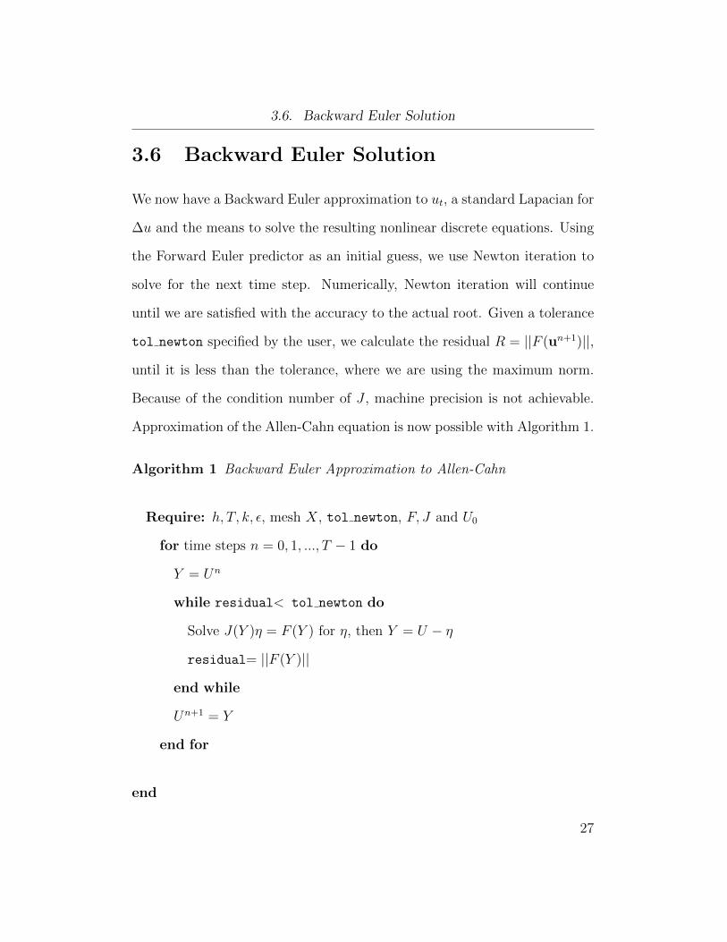
Approximation of the Allen-Cahn equation is now possible with Algorithm 1.
Algorithm 1 Backward Euler Approximation to Allen-Cahn
Require: h, T, k, ε, mesh X, tol newton, F, J and U0
for time steps n = 0, 1, ..., T − 1 do
Y = Un
while residual< tol newton do
Solve J(Y )η = F (Y ) for η, then Y = U − η
residual= ||F (Y )||
end while
Un+1 = Y
end for
end
27

3.7. Convergence
In section 3.2 we calculated using Taylor series that the BE method is first
order in time, and in section 3.3 that FD is second order in space. We now
can confirm these results by explicitly calculating the order of convergence.
3.7 Convergence
Suppose we had an exact solution u to our PDE and our approximation to
that exact solution u. The global error Ei is the absolute value of the dif-
ference between the true solution and the exact solution at each mesh point.
Our method is said to converge if this error vanishes as h → 0 and k → 0.
The order of the error is then the order of the method. In this case, we have
O(k) error from Backward Euler and O(h2) error from finite difference. Then
the total error in our current method is E = O(k) + O(h2). For one step in
this method, the local truncation error is O(k2) + O(kh2). This is the error
associated with the approximation to the derivatives as we calculated earlier
in this chapter. The local truncation error is different than the global error,
that is, each time step introduces a local error. The first O(k2) error comes
from the time derivative approximation from (3.7) where the truncated Tay-
lor series has the error term k2
2utt(tn) ≈ O(k2) for one step. The second
O(kh2) term comes from the spatial second derivative approximation from
(3.10) where the truncated Taylor series has the error term h2
4!uxxxx(xi, tn)
for one step and is multiplied by k in the discrete equation.
28
3.7. Convergence
We now use our code to show that our Backward Euler method is indeed
first order in time and second order in space. To check first order in time, we
fix the number of mesh points. This is done so that the spatial error O(h2)
remains constant and will not affect convergence. We then divide the time
step successively by 2. The error is calculated by taking the maximum norm
of each successive approximations and comparing the ratio. The ratio for the
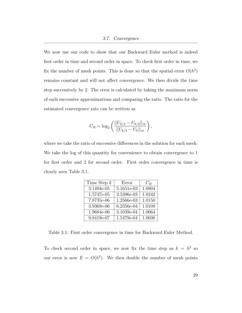
estimated convergence rate can be written as
CR = log2
(||Uk/4 − Uk/2||∞||Uk/2 − Uk||∞
),
where we take the ratio of successive differences in the solution for each mesh.
We take the log of this quantity for convenience to obtain convergence to 1
for first order and 2 for second order. First order convergence in time is
clearly seen Table 3.1.
Time Step k Error CR3.1494e-05 5.1651e-03 1.08041.5747e-05 2.5396e-03 1.02427.8735e-06 1.2566e-03 1.01503.9368e-06 6.2356e-04 1.01091.9684e-06 3.1039e-04 1.00649.8419e-07 1.5479e-04 1.0038
Table 3.1: First order convergence in time for Backward Euler Method.
To check second order in space, we now fix the time step as k = h2 so
our error is now E = O(h2). We then double the number of mesh points
29
3.8. Adaptive Time Stepping
successively. Similarly, the error is calculated by taking the maximum norm
of each successive approximations and comparing the ratio. The estimate for
the convergence rate can be written as
CR = log2
(||Uh/4 − Uh/2||∞||Uh/2 − Uh||∞
).
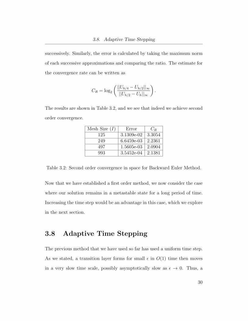
The results are shown in Table 3.2, and we see that indeed we achieve second
order convergence.
Mesh Size (I) Error CR125 3.1309e-02 3.3054249 6.6459e-03 2.2361497 1.5605e-03 2.0904993 3.5452e-04 2.1381
Table 3.2: Second order convergence in space for Backward Euler Method.
Now that we have established a first order method, we now consider the case
where our solution remains in a metastable state for a long period of time.
Increasing the time step would be an advantage in this case, which we explore
in the next section.
3.8 Adaptive Time Stepping
The previous method that we have used so far has used a uniform time step.
As we stated, a transition layer forms for small ε in O(1) time then moves
in a very slow time scale, possibly asymptotically slow as ε → 0. Thus, a
30
3.9. Local Error Method
uniform time step method will be inefficient in this part of the computation.
For small enough ε the transition layer will move slowly enough that an in-
ordinate number of time steps are required to resolve the dynamics.
To reduce the amount of work required, adaptivity in time should be used for
these problems. This is enabled by computing a local error estimate (LEE)
for each time step. If this LEE is within a tolerance that we have chosen, we
accept the solution for the current time step and increase the next time step.
And if this tolerance is violated, we decrease the time step. This method is
described in the local error method.
3.9 Local Error Method
We estimate the LEE for each time step to justify whether the solution should
be accepted and then determine the next time step. The time step will then
evolve with the dynamics of the solution, allowing us to compute the solution
efficiently far in time through the slow dynamics of the transition. We will
use the uniform time step solution as our basis of comparison to the methods
outlined in this chapter. The general algorithm of an adaptive time step
method is:
1. Calculate the next time step.
2. Compute the LEE.
31
3.9. Local Error Method
3. Accept/Reject the solution and adjust the time step.
An estimate of the LEE is found by the local error method [22]. The LEE,
denoted as δ, is given by the difference between two solutions, a predictor
and a corrector. The corrector solution will be our BE method, our intended
solution to the next time step. The predictor solution should be a best guess,
with the most efficient and quickest method to calculate the next time step.
This will be given by the Forward Euler method, an explicit and easy to
calculate solution. We then calculate a BE-FE pair for each time step. Then
the LEE is given by (3.9).
We can now adjust the time step to make δ smaller than the user speci-
fied tolerance δtol =tol delta. At each time step, we allow an increase in
the time step k by a factor of ξ or decrease by a factor of 1ξ, for ξ to be
determined. Suppose δ is smaller than δtol, we would like to increase k by
the highest amount without violating the tolerance inequality that we are
currently satisfying for the next time step. We need to determine ξ such that
δn+1 → ξp+1δn,
where p is the order of the method, p = 1 for the BE time stepping described
so far. The reason that ξ has the power p+ 1 is because the local truncation
error is of order kp+1.
32

3.9. Local Error Method
If we require that δ < 1γδtol, γ > 1, for a user defined γ, which then warrants
an increase in k, then by multiplying kn+1 = γ1/(p+1)kn will result in the next
δ to be near δtol. To make sure we are not too close to δtol we introduce the
safety factor θ = 0.8. Then ξ will be
ξ = p+1√θγ.
We determine the action to take after each time step with the following
algorithm similar to [22].
• if δδtol
< 1γ. Accept u, kn+1 = ξkn (Increase time step).
• else if δδtol∈[
1γ, 1)
. Accept u, kn+1 = kn (Keep the same time step).
• else, Reject u, kn = 1ξkn (Reduce time step).
We take this approach rather than smoothly varying k because we will con-
sider higher order multi step methods in later sections which require fixed
time steps to be efficient. When γ is increased, there is a decrease in the
number of instances we adjust the time step, however more time steps would
be required. For example, if we take γ = 2 and apply it to our BE-FE so-
lution for Allen-Cahn, the evolution of the time step is shown in Figure 3.2
compared to γ = 4.
33

3.9. Local Error Method
Figure 3.2: Backward Euler Solution with γ = 2 vs. γ = 4 in 1D.
In the context of a first order method, we only require one previous time
step. Thus there is no consequence to the previous data in increasing or
decreasing the time step. Figure 3.3 shows the number of time steps required
and number of times we increase or decrease k as we vary γ.
34
3.9. Local Error Method
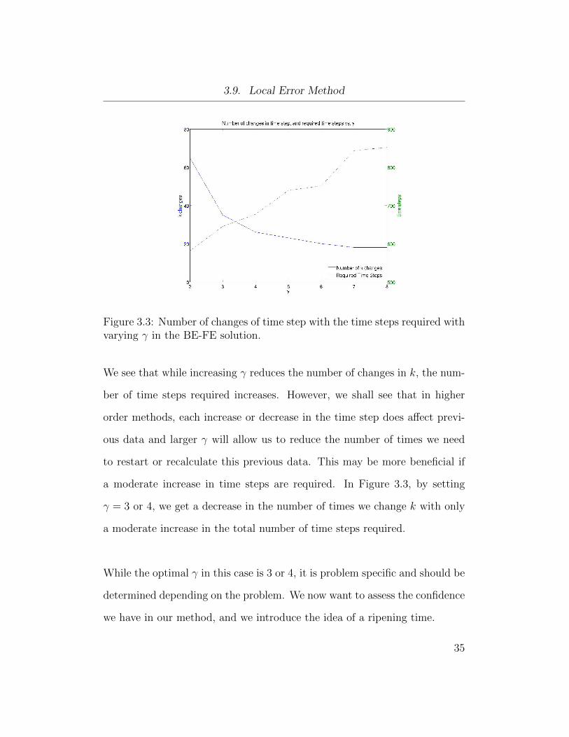
Figure 3.3: Number of changes of time step with the time steps required withvarying γ in the BE-FE solution.
We see that while increasing γ reduces the number of changes in k, the num-
ber of time steps required increases. However, we shall see that in higher
order methods, each increase or decrease in the time step does affect previ-
ous data and larger γ will allow us to reduce the number of times we need
to restart or recalculate this previous data. This may be more beneficial if
a moderate increase in time steps are required. In Figure 3.3, by setting
γ = 3 or 4, we get a decrease in the number of times we change k with only
a moderate increase in the total number of time steps required.
While the optimal γ in this case is 3 or 4, it is problem specific and should be
determined depending on the problem. We now want to assess the confidence
we have in our method, and we introduce the idea of a ripening time.
35
3.10. Ripening Time
3.10 Ripening Time
The ripening time Tr is a chosen moment in the dynamics of the solution that
will allow us to compare to other methods. In the case of the Allen-Cahn or
Cahn-Hilliard equations, with the appropriate initial condition, the solution
will have a region that quickly forms transition layers from the u = +1 to
u = −1 regions. As the transition layers move through time, the regions will
start to move toward the dominate region. In our cases, smaller regions in
the u = −1 regime eventually cross the zero axis into the u = +1 regime.
The moment this happens, we call the ripening time. This can be monitored
by looking at the minimum of our current solution. As we let δtol → 0
we expect these ripening time estimates to converge, corresponding to our
solution converging to a accurate solution. We also expect the number of
time steps M(δtol) required to follow linearly as M(δtol/10)M(δtol)
= p+1√
10, where
p is the order of the method, in this case p = 1. This is because as we
decrease δtol by a factor of 10, the error we had would be δold ≈ Ckp+1 and
the next error will be δnew ≈ C(νk)p+1 = νp+1Ckp+1 = νp+1δold, for constant
ν. Thus to reduce the local error by a factor of 10, the time step size should
be reduced by a factor of about p+1√
10. The results of this numerical test
for the Allen-Cahn problem to be presented in the next section are shown in
Table 3.3.
36

3.11. Numerical Experiment - Allen-Cahn
δtol Tr M(δtol)M(δntol)
M(δn−1tol )
1.0000e-04 541.8487 645 3.08611.0000e-05 545.2975 2,000 3.10081.0000e-06 546.2953 6,275 3.13751.0000e-07 546.6366 20,169 3.21421.0000e-08 546.7448 62,480 3.09781.0000e-09 546.7788 199,630 3.1951
Table 3.3: Convergence of the ripening time for Allen-Cahn using BE-FEtime stepping method.
We see that our solution converges to Tr = 546.8 and as we expected, the
ratio of M(δtol) also converges close to 2√
10 = 3.1622, and we thus confident
in to application of our method to this problem. We will use these results to
compare to our higher-order methods.
3.11 Numerical Experiment - Allen-Cahn
For Allen-Cahn, after we have passed the ripening time, the solution will
then evolve to a steady state, and in our case it will be u = 1. Our initial
condition is u0(x) = sinx + 0.8 on [0, 2π]. This is chosen so that the region
above u = 0 is slightly larger than below u = 0 which avoids symmetry.
We are interested in the case where we have a dominant region, and the
subdominant region is eventually absorbed. The parameters we have chosen
37

3.11. Numerical Experiment - Allen-Cahn
are
ε = 0.16, n = 128,
T = 537, tol delta = 10−4,
θ = 0.8, tol newton = 10−8,
γ = 3, u0(x, 0) = sin(x) + 0.8.
.
As we begin the simulation, we expect the initial dynamics to require small
time steps as the transition layer is formed. Figure 3.4 shows the evolution
of the solution as we form the transition layer, metastable state and then
reach the stable state.
Figure 3.4: BE-FE Solution with Adaptive Time Stepping for Allen-Cahn in1D for f(x) = sin(x) + 0.8 on [0, 2π].
We see the fast dynamics from the initial condition to the metastable state,
where two transition layers are formed. Then, during the metastable state
the time step k is rapidly increased as shown in Figure 3.5.
38

3.11. Numerical Experiment - Allen-Cahn
Figure 3.5: BE-FE Solution - Evolution of time step k vs time t for Allen-Cahn.
We see rapid growth initially and gradual decline as we leave the metastable
state. The total number of time steps for this experiment was 811. We will
show a comparison to the uniform method in the next section. We also plot
the Liapunov energy (1.4) to show that we indeed are reducing the energy in
time, and the number of Newton iterations, shown in Figure 3.6, where the
average number of iterations is 3.39, with a maximum of 11.
39
3.11. Numerical Experiment - Allen-Cahn
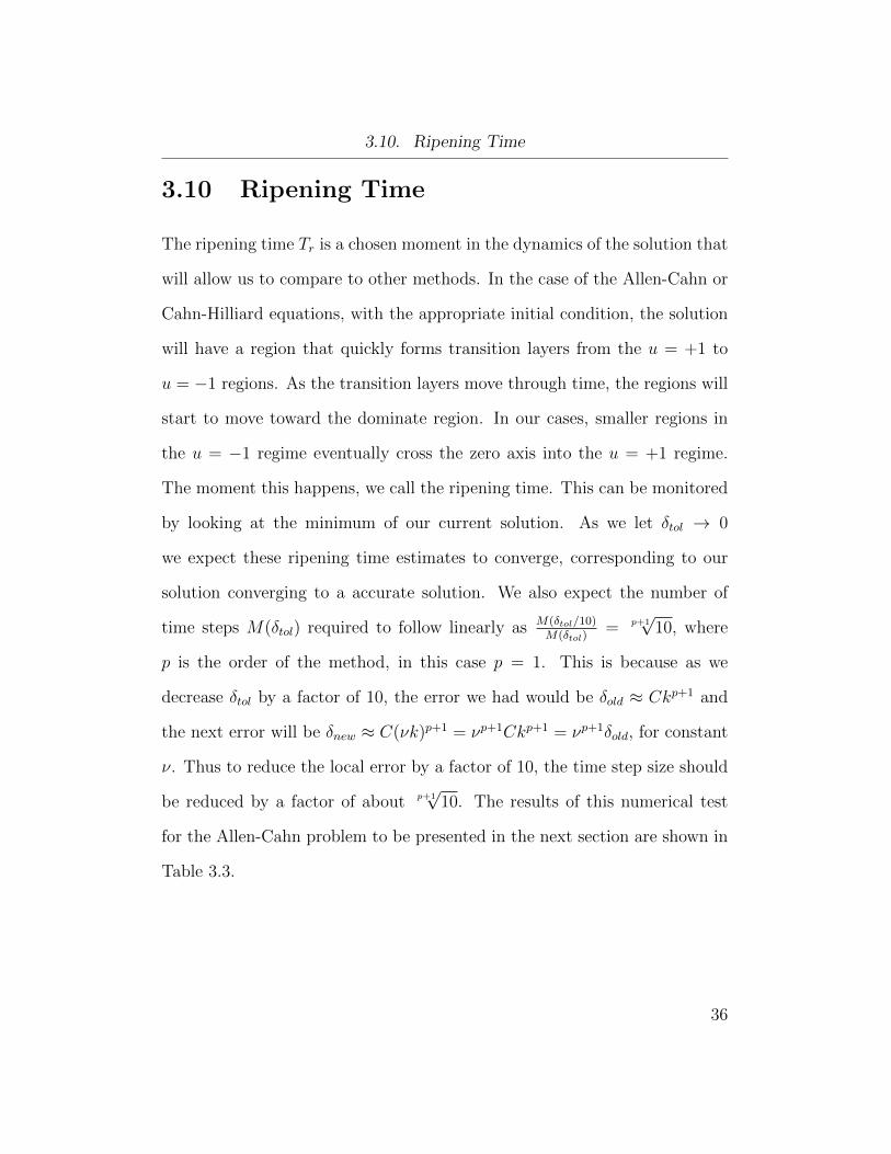
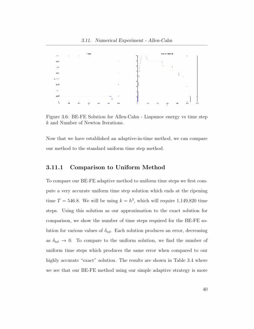
Figure 3.6: BE-FE Solution for Allen-Cahn - Liapunov energy vs time stepk and Number of Newton Iterations.
Now that we have established an adaptive-in-time method, we can compare
our method to the standard uniform time step method.
3.11.1 Comparison to Uniform Method
To compare our BE-FE adaptive method to uniform time steps we first com-
pute a very accurate uniform time step solution which ends at the ripening
time T = 546.8. We will be using k = h3, which will require 1,149,820 time
steps. Using this solution as our approximation to the exact solution for
comparison, we show the number of time steps required for the BE-FE so-
lution for various values of δtol. Each solution produces an error, decreasing
as δtol → 0. To compare to the uniform solution, we find the number of
uniform time steps which produces the same error when compared to our
highly accurate “exact” solution. The results are shown in Table 3.4 where
we see that our BE-FE method using our simple adaptive strategy is more
40

3.12. Numerical Experiment - Cahn-Hilliard
efficient than uniform time steps as we let δtol → 0.
δtol Error||uadap−uexact||
Time steps(Adaptive)
Error||uuni−uexact||
Time steps(Uniform)
1.0000e-04 7.9679e-01 657 7.9691e-01 5161.0000e-05 1.0668e-01 1,700 1.0657e-01 6,7751.0000e-06 3.3542e-02 5,239 3.3525e-02 21,2701.0000e-07 1.2659e-02 16,627 1.2667e-02 49,415
Table 3.4: Required number of time steps for BE-FE vs uniform for decreas-ing δtol.
As we expected, our problem contains a significant length of time where the
solution is in the metastable state and no dynamics are occurring, and we see
the reduction in time steps required for the adaptive method which increases
the step rapidly during this time. This is the most prominent gain over the
uniform method. We can also apply this method to the other equation we
are investigating, the Cahn-Hillard equation.
3.12 Numerical Experiment - Cahn-Hilliard
The Cahn-Hilliard equation is volume or mass preserving, and we expect
qualitatively different dynamics. We look at problem (1.3), which is fourth-
order in space, where the discretization is now
Un+1 − Un
k= −ε2∆2
hUn+1 + ∆hw
′(Un+1).
41

3.12. Numerical Experiment - Cahn-Hilliard
with ∆2h the Biharmonic operator. Our method that we applied to the Allen-
Cahn problem will extend to this problem in the same manner. Our initial
condition is u0(x, t) = cos(2x) + 0.01ecos(x+0.1) on [0, 2π]. This is chosen to
have two similar regions with one slightly smaller than the other. We are
interested in the case where the two regions will eventually absorb into one
region. The parameters we have chosen are
ε = 0.22, n = 128,
T = 1, 033, tol delta = 10−4,
θ = 0.8, tol newton = 10−8,
γ = 3, u0(x, 0) = cos(2x) + 0.01ecos(x+0.1).
.
This configuration demonstrates the two separate regions, as we see that both
regions will eventually be absorbed together as we observe in Figure 3.7.
Figure 3.7: BE-FE Solution with Adaptive Time Stepping for Cahn-Hilliardin 1D for f(x) = cos(2x) + 0.01ecos(x+0.1) on [0, 2π].
42

3.12. Numerical Experiment - Cahn-Hilliard
As we have seen in the Allen-Cahn case, we also see the fast dynamics
from the initial condition to the metastable state, where transition layers
are formed. Since one region is slightly smaller than the other, we expect the
time step k to be increased rapidly as shown in Figure 3.8.
Figure 3.8: BE-FE Solution - Evolution of time step k vs time t for Cahn-Hilliard.
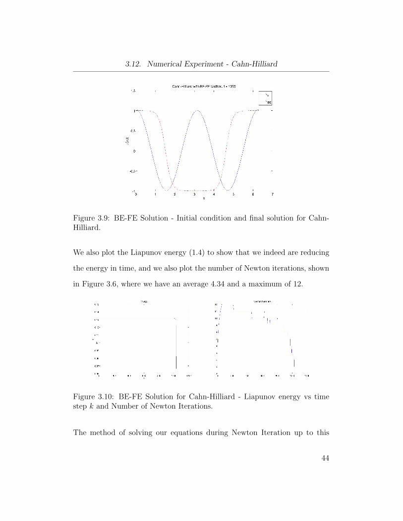
The final result occurs when the center transition layer is eventually ab-
sorbed, shown in Figure 3.9 where both regions have joined together.
43
3.12. Numerical Experiment - Cahn-Hilliard
Figure 3.9: BE-FE Solution - Initial condition and final solution for Cahn-Hilliard.
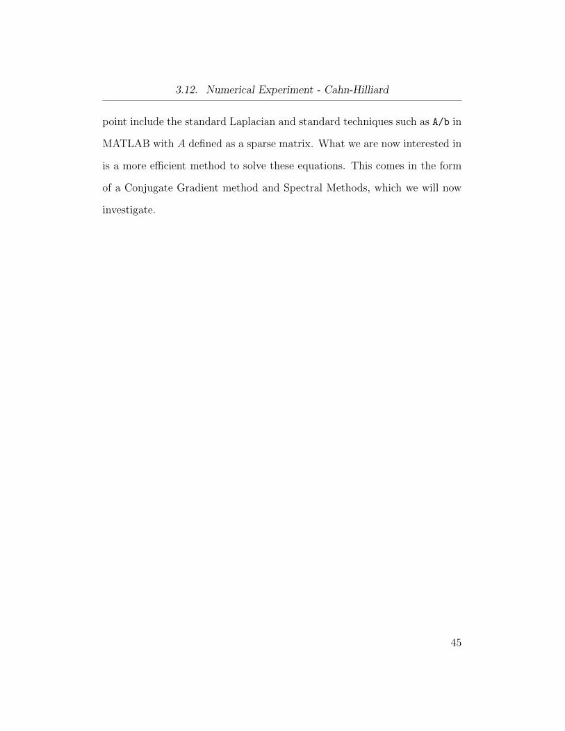
We also plot the Liapunov energy (1.4) to show that we indeed are reducing
the energy in time, and we also plot the number of Newton iterations, shown
in Figure 3.6, where we have an average 4.34 and a maximum of 12.
Figure 3.10: BE-FE Solution for Cahn-Hilliard - Liapunov energy vs timestep k and Number of Newton Iterations.
The method of solving our equations during Newton Iteration up to this
44
3.12. Numerical Experiment - Cahn-Hilliard
point include the standard Laplacian and standard techniques such as A/b in
MATLAB with A defined as a sparse matrix. What we are now interested in
is a more efficient method to solve these equations. This comes in the form
of a Conjugate Gradient method and Spectral Methods, which we will now
investigate.
45
Chapter 4
Solution Techniques
In this chapter we look at the Conjugate Gradient (CG) method and employ
our preconditioner for Preconditioned CG (PCG). In Section 3.5, we solve a
linear system of equations for each time step. The CG method is an iterative
method that is potentially an efficient method to solve the system
Ax = b,
where A is symmetric positive definite (spd), where all the entries are real.
That is, for an n × n matrix A, it is symmetric (AT = A), positive definite
(xTAx > 0) ∀ nonzero vectors x ∈ Rn. The specific system we will be
solving is given in (3.12). The CG method is in a class called Krylov subspace
methods. We will give brief background and then present the CG algorithm
as this method plays a central role in the methods presented in this thesis.
4.1 Conjugate Gradient
For a small and dense linear system, direct methods would be the most effi-
cient solution to the system. However, in the case of simulating solid cancer
46

4.1. Conjugate Gradient
tumor growth [15], for example, the system is very large and sparse where
iterative methods will be the most efficient [23].
Krylov subspace methods, [23, 24, 25], are intended to iteratively converge
to the solution to the system Ax = b when A ∈ Rn×n. The approxima-
tions are in a Krylov subspace, which is a subspace spanned by vectors of
the form p(A)v where p is a polynomial of degree up to k − 1. That is, for
any real, n × n nonsingular matrix A and vector b of the same length, the
k-dimensional Krylov Subspace of A with respect to b is defined by the space
spanned by powers of A, written as Kk(A,b) = spanb, Ab, A2b, ..., Ak−1b
[26]. Then, the solution to our system x = A−1b can be solved in a more
efficient manner by approximating A−1b with p(A)b, an element of this sub-
space.
The CG method is in a class called gradient descent where we can write
the iteration as
xk+1 = xk + αkpk,
where pk is known as the search direction and
αk =〈rk, rk〉〈pk, Apk〉
47

4.1. Conjugate Gradient
is the step size, where 〈x,y〉 = xTy is the inner product [26]. In terms of a
Krylov subspace, we have xk ∈ Kk and pk ∈ Kk+1. The idea behind gradient
descent is that the search direction is found by taking the gradient or find
the minimizer of
φ(x) =1
2xTAx− bTx.
If we take the gradient of φ(x) we get r = b − Ax which is known as the
residual [26]. If our initial guess was x0 = 0, then our first search direction
will be p1 = b. In the CG method, we require that the remaining pk are
each orthogonal, or conjugate to this gradient, which gives its name. The
main feature of pk is that they are A-conjugate, namely that pTkApj = 0 for
k 6= j [26]. The next search direction is a linear combination of the previous
search direction and current residual as
pk+1 = rk+1 + βkpk
for βk calculated in [26], given by
βk =〈rk+1, rk+1〉〈rk, rk〉
.
Full details into the derivation and discussion about CG can be found in
[26, 23]. The conjugate gradient method is given in Algorithm 2.
Algorithm 2 Conjugate Gradient Method
48

4.2. Preconditioning
Require: r0 = b− Ax0, p0 = r0
for k = 0, 1, ..., until convergence do
αk = 〈rk, rk〉/〈pk, Apk〉
xk+1 = xk + αkpk
rk+1 = rk − αkApk
βk = 〈rk+1, rk+1〉/〈rk, rk〉
pk+1 = rk+1 − βkpk
end for
end
4.2 Preconditioning
Preconditioning is the method by which a matrix P is applied as a trans-
formation to our problem Ax = b which gives a more suitable problem to
solve. This is related to the condition number of the matrix A. The condition
number κ(A) of A, is the ratio of the maximum and minimum eigenvalues
of A. If κ(A) is large, the number of iterations required to converge to the
solution can also be large. In general, the number of CG iterations to reach
a specific residual tolerance is O(√
κ(A))
. Even if the condition number
is large, convergence better than this generic result can be obtained if the
eigenvalues are well clustered. A preconditioner P used in the CG algorithm
will be a spd matrix such that P−1 approximates the inverse of A. Then our
CG method would solve a problem where the matrix P−1A has a lower con-
49
4.2. Preconditioning
dition number, preferably with eigenvalues clustered near 1. Our CG method
with preconditioning is now shown in Algorithm 3.
Algorithm 3 Preconditioned Conjugate Gradient Method
Require: r0 = b− Ax0, Pp0 = r0
for k = 0, 1, ..., until convergence do
αk = 〈rk, rk〉/〈pk, Apk〉
xk+1 = xk + αkpk
rk+1 = rk − αkApk
βk = 〈rk+1, rk+1〉/〈rk, rk〉
Solve Py = rk+1 for y
pk+1 = y − βkpk
end for
end
If we want to employ a standard preconditioner to our iterative method, such
as Incomplete LU (ILU), it would have to be calculated for each Newton step.
This is because the Jacobian changes for each iteration. This is very ineffi-
cient, and we would like to use a preconditioner that avoids calculation at
every iteration for each implicit time step. We can employ a linear model
preconditioner as suggested to us by Scott MacLachlan. Consider (3.12),
the implicit problem to be solved at each time step for the discretization of
the Allen-Cahn Equation (1.2). For each Newton iteration, the next iterate
50
4.2. Preconditioning
requires a solve with the Jacobian coefficient matrix given in (3.14).
The matrix J is dense but symmetric and multiplication by J can be done ef-
ficiently using the fast Fourier transform and diagonal multiplication, which
leads to our use of CG as a solution technique. We use the preconditioner
P−1 where P is the discretization of the constant coefficient problem
P = I − kε2∆h + 2kI, (4.1)
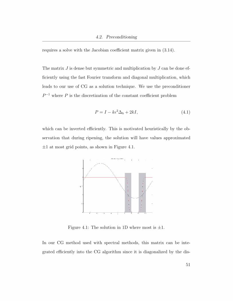
which can be inverted efficiently. This is motivated heuristically by the ob-
servation that during ripening, the solution will have values approximated
±1 at most grid points, as shown in Figure 4.1.
Figure 4.1: The solution in 1D where most is ±1.
In our CG method used with spectral methods, this matrix can be inte-
grated efficiently into the CG algorithm since it is diagonalized by the dis-
51
4.2. Preconditioning
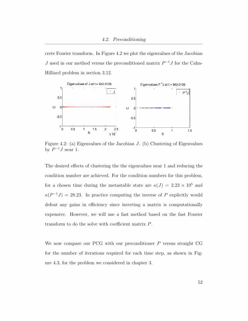
crete Fourier transform. In Figure 4.2 we plot the eigenvalues of the Jacobian
J used in our method versus the preconditioned matrix P−1J for the Cahn-
Hilliard problem in section 3.12.
Figure 4.2: (a) Eigenvalues of the Jacobian J . (b) Clustering of Eigenvaluesby P−1J near 1.
The desired effects of clustering the the eigenvalues near 1 and reducing the
condition number are achieved. For the condition numbers for this problem,
for a chosen time during the metastable state are κ(J) = 2.23 × 10⁵ and
κ(P−1J) = 28.23. In practice computing the inverse of P explicitly would
defeat any gains in efficiency since inverting a matrix is computationally
expensive. However, we will use a fast method based on the fast Fourier
transform to do the solve with coefficient matrix P .
We now compare our PCG with our preconditioner P versus straight CG
for the number of iterations required for each time step, as shown in Fig-
ure 4.3, for the problem we considered in chapter 3.
52
4.2. Preconditioning
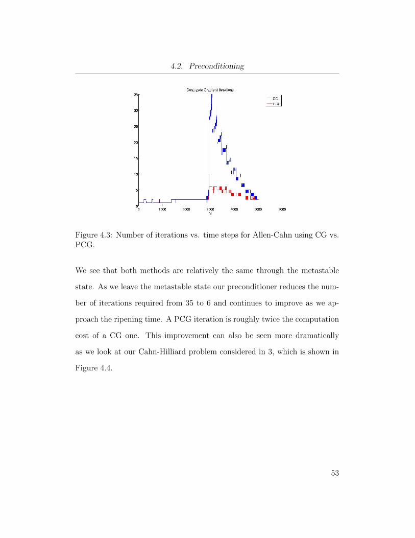
Figure 4.3: Number of iterations vs. time steps for Allen-Cahn using CG vs.PCG.
We see that both methods are relatively the same through the metastable
state. As we leave the metastable state our preconditioner reduces the num-
ber of iterations required from 35 to 6 and continues to improve as we ap-
proach the ripening time. A PCG iteration is roughly twice the computation
cost of a CG one. This improvement can also be seen more dramatically
as we look at our Cahn-Hilliard problem considered in 3, which is shown in
Figure 4.4.
53

4.2. Preconditioning
Figure 4.4: Number of CG iterations vs. Time steps for Cahn-Hilliard usingCG vs. PCG.
Here we see a significant reduction of iterations required, from 13922 to 689,
and continues to improve during the metastable state. The linear model pre-
conditioner suggested to us by Scott MacLachlan has allowed us to improve
our CG by reducing the number of iterations to converge, which for the thou-
sands of time steps required for both problems, presents an advantage as we
notice a significant speed up when we run our programs. As we stated, our
preconditioner is diagonalized through the fast Fourier transform, therefore
we now investigate spectral methods to improve our solution and provide an
efficient spatial discretization to our problem.
54
Chapter 5
Spectral Methods in Space
Spectral methods are a class of numerical methods to solve differential equa-
tions, usually including the Fast Fourier Transform. They were introduced
by Steven Orszag in 1969 [10]. While they are fast to compute, they also
have the best possible error properties for our application, specifically called
spectral accuracy. We will give a simplified introduction to Spectral Methods
below. The material in this chapter is largely adapted from [12].
As we have seen in Chapter 3, the finite difference approximations we make
of the derivatives in a differential equation at a point xj are found using the
neighbouring points in the mesh. If we are given initial data U = u1, ...uI
at each point xj = x1, ..., xI in the domain, then we can approximate
the derivatives in this fashion. For example, our familiar second derivative
approximation of u at xj, u′′j = u′′j (xj) is
u′′j ≈uj+1 − 2uj + uj−1
h2
55
Chapter 5. Spectral Methods in Space
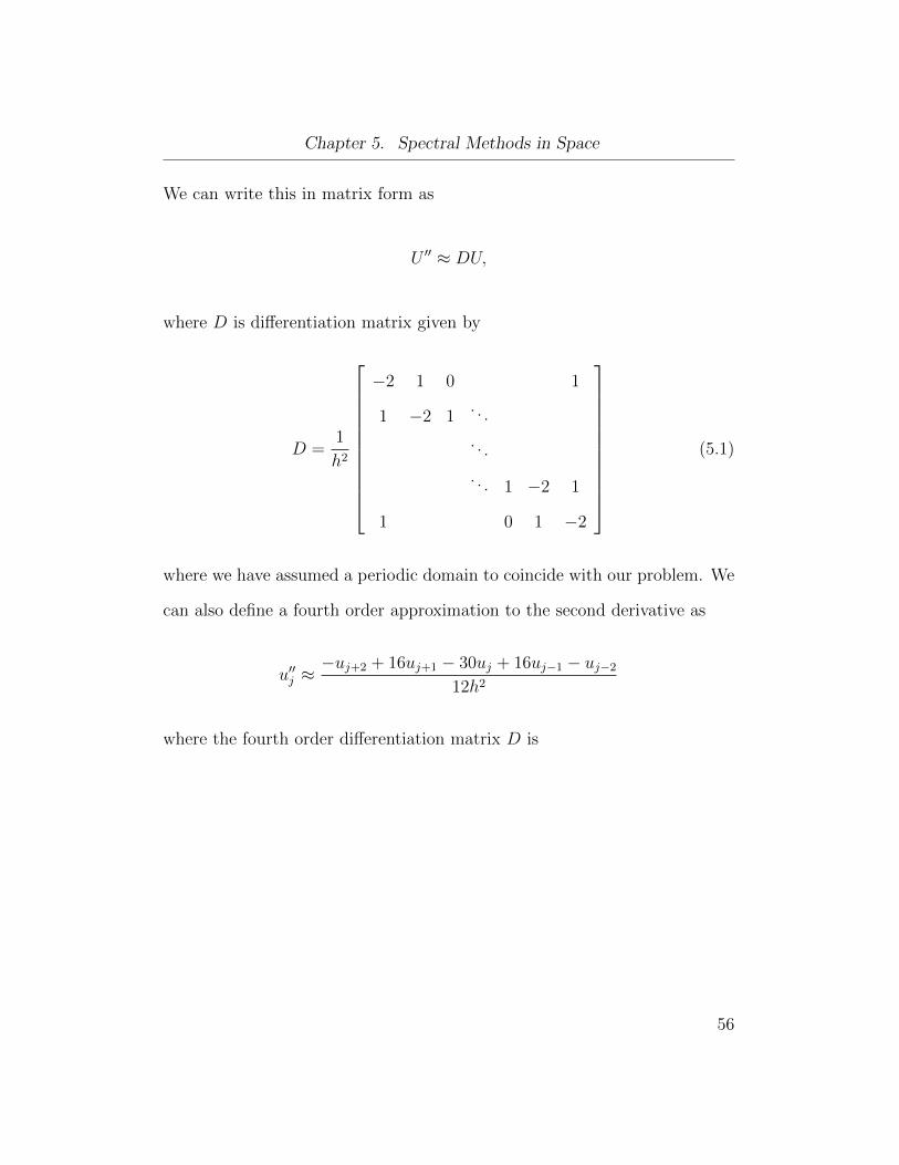
We can write this in matrix form as
U ′′ ≈ DU,
where D is differentiation matrix given by
D =1
h2
−2 1 0 1
1 −2 1. . .
. . .
. . . 1 −2 1
1 0 1 −2
(5.1)
where we have assumed a periodic domain to coincide with our problem. We
can also define a fourth order approximation to the second derivative as
u′′j ≈−uj+2 + 16uj+1 − 30uj + 16uj−1 − uj−2
12h2
where the fourth order differentiation matrix D is
56
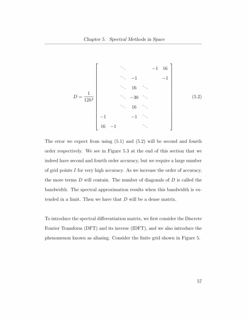
Chapter 5. Spectral Methods in Space
D =1
12h2
. . . −1 16
. . . −1 −1
. . . 16. . .
. . . −30. . .
. . . 16. . .
−1 −1. . .
16 −1. . .
(5.2)
The error we expect from using (5.1) and (5.2) will be second and fourth
order respectively. We see in Figure 5.3 at the end of this section that we
indeed have second and fourth order accuracy, but we require a large number
of grid points I for very high accuracy. As we increase the order of accuracy,
the more terms D will contain. The number of diagonals of D is called the
bandwidth. The spectral approximation results when this bandwidth is ex-
tended in a limit. Then we have that D will be a dense matrix.
To introduce the spectral differentiation matrix, we first consider the Discrete
Fourier Transform (DFT) and its inverse (IDFT), and we also introduce the
phenomenon known as aliasing. Consider the finite grid shown in Figure 5.
57
Chapter 5. Spectral Methods in Space
· · · t t t t t t t tx1 xI/2 xI
2ππ0 ︷ ︸︸ ︷h
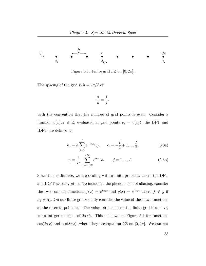
Figure 5.1: Finite grid hZ on [0, 2π].
The spacing of the grid is h = 2π/I or
π
h=I
2.
with the convention that the number of grid points is even. Consider a
function v(x), x ∈ Z, evaluated at grid points vj = v(xj), the DFT and
IDFT are defined as
vα = hI∑j=1
e−iαxjvj, α = −I2
+ 1, ...,I
2, (5.3a)
vj =1
2π
I/2∑α=−I/2
eiαxj vk, j = 1, ..., I. (5.3b)
Since this is discrete, we are dealing with a finite problem, where the DFT
and IDFT act on vectors. To introduce the phenomenon of aliasing, consider
the two complex functions f(x) = eiα1x and g(x) = eiα2x where f 6= g if
α1 6= α2. On our finite grid we only consider the value of these two functions
at the discrete points xj. The values are equal on the finite grid if α1 − α2
is an integer multiple of 2π/h. This is shown in Figure 5.2 for functions
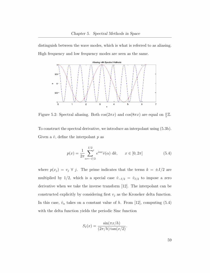
cos(2πx) and cos(8πx), where they are equal on π5Z on [0, 2π]. We can not
58
Chapter 5. Spectral Methods in Space
distinguish between the wave modes, which is what is referred to as aliasing.
High frequency and low frequency modes are seen as the same.
Figure 5.2: Spectral aliasing. Both cos(2πx) and cos(8πx) are equal on π5Z.
To construct the spectral derivative, we introduce an interpolant using (5.3b).
Given a v, define the interpolant p as
p(x) =1
2π
I/2∑′
α=−I/2
eiαxv(α) dk, x ∈ [0, 2π] (5.4)
where p(xj) = vj ∀ j. The prime indicates that the terms k = ±I/2 are
multiplied by 1/2, which is a special case v−I/2 = vI/2 to impose a zero
derivative when we take the inverse transform [12]. The interpolant can be
constructed explicitly by considering first vj as the Kroneker delta function.
In this case, vα takes on a constant value of h. From [12], computing (5.4)
with the delta function yields the periodic Sinc function
SI(x) =sin(πx/h)
(2π/h) tan(x/2).
59
Chapter 5. Spectral Methods in Space
This interpolation is a translation-invariant process in the sense that for any
m, the interpolant of δj−m is SI(x− xm) [12]. Then a linear combination of
translated Sinc functions can also be written to describe the interpolant
p(x) =1
2π
I∑j=1
vjSI(x− xj).
To find the spectral second derivative matrix, we simply compute the second
derivative of SI(x).
S ′′I (xj) =
−π2
3h2− 1
6, j ≡ 0 (mod I),
12(−1)j csc2(jh/2), j 6= 0 (mod I).
And the second derivative matrix D can be written as
D(2)I =
1
h
...
−12
csc2 3h2
. . . 12
csc2 h
. . . 12
csc2 h2
. . . − π2
3h2− 1
6
. . .
12
csc2 h2
. . .
−12
csc2 h. . .
12
csc2 3h2
...
(5.5)
Now using (5.5) as our approximation to the second derivative, we see in
60

Chapter 5. Spectral Methods in Space
Figure 5.3 that the approximation to the second derivative of f(x) = esinx
achieves very high accuracy with a significantly less number of grid points
compared to (5.1) and (5.2) up to 1012. What we observe once N > 30 is
an accuracy that has reached machine precision. Therefore we can choose
a much smaller N than our standard methods, and any larger N will not
achieve any better accuracy, as shown in the cloud of data points in Fig-
ure 5.3.
Aliasing is the only source of error in this approach, small for C∞ func-
tions because v(α) decays like 1/αp for every vj ∈ C∞. Such a high accurate
approximation is limited by machine precision and no further improvement
is possible. It can be shown that the approximation is asymptotically better
than any fixed convergence order when applied to smooth (C∞) functions
[12]. This is what is referred to as spectral accuracy. In contrast to finite
differences, where the error decreases like O(hp) for a p-order approximation,
we achieve O(hp) convergence for any p assuming the solution is infinitely dif-
ferentiable. The spectral differentiation matrix is diagonalized by the DFT,
which is evaluated efficiently using the FFT. And using Newton iteration, we
can solve our problem as we have before now with the spectral differentiation
matrix.
61

5.1. Using the Fast Fourier Transform
Figure 5.3: Spectral order accuracy versus Finite Difference, on a test prob-lem for the second derivative of f(x) = esinx taken as a periodic function on[0, 2π].
5.1 Using the Fast Fourier Transform
Instead of using the full spectral differentiation matrix (5.5), we can use the
FFT and IFFT to compute approximations of second derivatives of u in a
faster way on the uniform grid with I grid points [13]. Recall the DFT in
(5.3a) and IFDT in (5.3b). We first obtain I discrete Fourier coefficients vα
by taking the FFT of uj on grid points xj. However, as stated, because of
aliasing the spectral method provides us with uj for |αj| ≤ I/2 and all other
62
5.1. Using the Fast Fourier Transform
modes of αj + I are indistinguishable on the grid. We write the vector α as
α =
(0, 1, ...,
I
2− 1,
I
2,−I
2+ 1, ...,−2,−1
).
In Fourier representation, differentiation is diagonal multiplication by iα.
Second derivatives are achieved by multiplication by −α2j . Second derivative
values are then obtained using the IFFT. To summarize,
D(2)I = F−1Λ2F,
where F is the matrix representation of the DFT and Λ2 is a diagonal matrix
with entries −α2j . Note that although D
(2)I is a full matrix, we can multiply
by D(2)I efficiently with this representation. This allows for efficient PCG
solution of the problems from implicit time stepping for our models.
63
Chapter 6
High-Order Time step
Techniques
In this chapter, we investigate higher order time stepping methods. Backward
Differentiation Formula (BDF) methods are often used for efficient solution
of stiff problems. For example, the MATLAB routine ode15s optionally uses
BDF techniques. We implement BDF time stepping of order 2 and 3 on
our problems, with order 2 and 3 Adams Bashforth explicit methods as our
predictor, and we will use implicit Runge-Kutta (RK) methods for initial
time steps and restarts when the time step is changed.
6.1 Runge Kutta Methods
Consider the initial value problem posed in (3.1). Following [28], Runge
considered the midpoint rule in 1895 to improve on the O(k) error of the
Euler Method. An intermediate Euler step between tn and tn + k with step
64
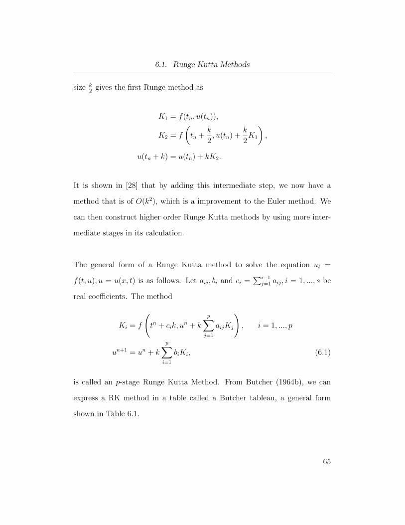
6.1. Runge Kutta Methods
size k2
gives the first Runge method as
K1 = f(tn, u(tn)),
K2 = f
(tn +
k
2, u(tn) +
k
2K1
),
u(tn + k) = u(tn) + kK2.
It is shown in [28] that by adding this intermediate step, we now have a
method that is of O(k2), which is a improvement to the Euler method. We
can then construct higher order Runge Kutta methods by using more inter-
mediate stages in its calculation.
The general form of a Runge Kutta method to solve the equation ut =
f(t, u), u = u(x, t) is as follows. Let aij, bi and ci =∑i−1
j=1 aij, i = 1, ..., s be
real coefficients. The method
Ki = f
(tn + cik, u
n + k
p∑j=1
aijKj
), i = 1, ..., p
un+1 = un + k
p∑i=1
biKi, (6.1)
is called an p-stage Runge Kutta Method. From Butcher (1964b), we can
express a RK method in a table called a Butcher tableau, a general form
shown in Table 6.1.
65
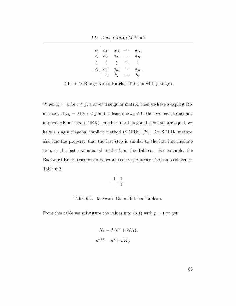
6.1. Runge Kutta Methods
c1 a11 a12 · · · a1p
c2 a21 a22 · · · a2p...
......
. . ....
cp ap1 ap2 · · · appb1 b2 · · · bp
Table 6.1: Runge Kutta Butcher Tableau with p stages.
When aij = 0 for i ≤ j, a lower triangular matrix, then we have a explicit RK
method. If aij = 0 for i < j and at least one aii 6= 0, then we have a diagonal
implicit RK method (DIRK). Further, if all diagonal elements are equal, we
have a singly diagonal implicit method (SDIRK) [29]. An SDIRK method
also has the property that the last step is similar to the last intermediate
step, or the last row is equal to the bi in the Tableau. For example, the
Backward Euler scheme can be expressed in a Butcher Tableau as shown in
Table 6.2.
1 11
Table 6.2: Backward Euler Butcher Tableau.
From this table we substitute the values into (6.1) with p = 1 to get
K1 = f (un + kK1) ,
un+1 = un + kK1,
66

6.1. Runge Kutta Methods
or, more simply as
un+1 = un + kf(un+1).
In our problem we will consider the SDIRK methods of order two and three
for use in our second and third order methods.
6.1.1 Singly Diagonal Implicit Runge Kutta 2
(SDIRK2)
For higher order multi-step methods described in section 6.2 it is usually re-
quired to have p previous values for a p order method. Runge Kutta methods
do not have this requirement. Therefore these methods are desirable, but are
computationally expensive due to the intermediate steps for only one time
step. Thus, we will use them to compute previous values needed for multi-
step methods initially and when the time step size changes. The Butcher
Tableau for SDIRK2 is given by
1 β 01 1− β β
1− β β
Table 6.3: SDIRK2 Butcher Tableau.
67

6.1. Runge Kutta Methods
From (6.1), this gives the formula
K1 = f(un + kβK1),
K2 = f(un + k(1− β)K1 + kβK2), β = 1−√
2
2,
un+1 = un + k[(1− β)K1 + βK2], (6.2)
where β is found as the root of the polynomial 12− 2β+β2. This polynomial
arises from the order conditions derived in [29], where each order of SDIRK
method consists of a p order polynomial to obtain β . Similar to Section
3.7 where we computed the convergence of the BE solution for the Allen-
Cahn equation, we can check that SDIRK2 is indeed second order in time of
O(k2). We divide the time step k by 2 successively with a fixed mesh, shown
in Table 6.4.
k Error CR6.0239e-04 1.6938e-06 2.00303.0120e-04 4.2301e-07 2.00151.5060e-04 1.0570e-07 2.00077.5299e-05 2.6419e-08 2.00043.7650e-05 6.6038e-09 2.0002
Table 6.4: Second order convergence in time for SDIRK2.
SDIRK2 will become very useful as a second order method in our adaptive
time stepping techniques. It allows us to compute initial conditions and
restart our methods while maintaining second order accuracy so that the
entire method is second order.
68
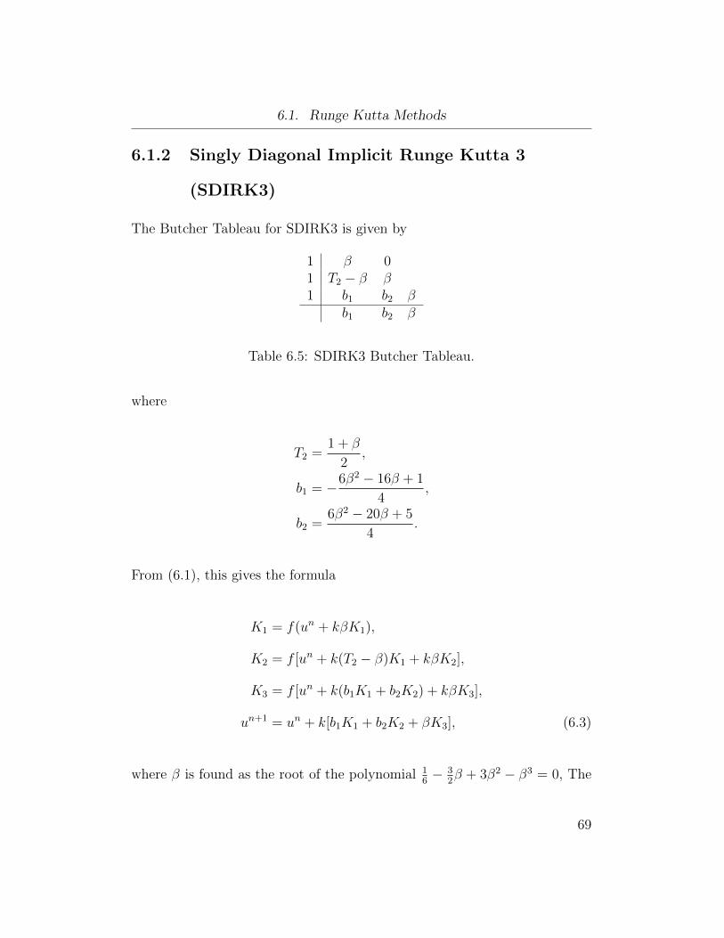
6.1. Runge Kutta Methods
6.1.2 Singly Diagonal Implicit Runge Kutta 3
(SDIRK3)
The Butcher Tableau for SDIRK3 is given by
1 β 01 T2 − β β1 b1 b2 β
b1 b2 β
Table 6.5: SDIRK3 Butcher Tableau.
where
T2 =1 + β
2,
b1 = −6β2 − 16β + 1
4,
b2 =6β2 − 20β + 5
4.
From (6.1), this gives the formula
K1 = f(un + kβK1),
K2 = f [un + k(T2 − β)K1 + kβK2],
K3 = f [un + k(b1K1 + b2K2) + kβK3],
un+1 = un + k[b1K1 + b2K2 + βK3], (6.3)
where β is found as the root of the polynomial 16− 3
2β + 3β2 − β3 = 0, The
69

6.1. Runge Kutta Methods
derivation of this formula is found in [29]. The root β to this equation will
be irrational, and up to 20 digits we have
β = 0.43586652150845899942.
Now we can check that this method is indeed third order in time of O(k3).
Again similar to Section 3.7 where we computed the convergence of the BE
solution for the Allen-Cahn equation, we look at the convergence of SDIRK3
for time step k by dividing k by 2 successively with a fixed mesh, shown in
Table 6.6.
k Error CR6.0239e-04 4.7413e-08 2.95313.0120e-04 6.0273e-09 2.97571.5060e-04 7.5990e-10 2.98767.5299e-05 9.5400e-11 2.99373.7650e-05 1.1952e-11 2.99671.8825e-05 1.4957e-12 2.9984
Table 6.6: Third order convergence in time for SDIRK3.
SDIRK3 will be used in our third order method for restarts to maintain
a fully third order method. Now we will consider our predictor, where we
require a second and third order explicit formulas to coincide with our second
and third order methods. We have chosen Adams Bashforth methods, which
are linear multi step methods.
70
6.2. Linear Multi Step Methods
6.2 Linear Multi Step Methods
A linear multi step method (LMM) of n steps requires the use of previous
information in the last n time steps. Using more than one previous time
step is different than RK methods, and we need a method to compute this
additional information. We will use implicit SDIRK methods to compute the
previous time steps needed for use with LMM’s. The general form of LMM’s
are
n∑j=0
ajun−j = kn∑j=0
bjfn−j
where n is the number of steps in the method, and aj, bj are coefficients
specific to the method.
6.2.1 Adams-Bashforth 2 (AB2)
Explicit LMM’s such as Adams-Bashforth (AB) solve the equation ut = f(u)
with
un+1 = un +
∫ tn
tn−1
f(t, u(t))dt,
where f(t, u(t)) is approximated by an explicit interpolation polynomial,
which does not involve the value of un+1. Hence, these are explicit meth-
ods that will only be used in the estimation our solution, as we will see in
our adaptive time stepping methods. For our second order method we will
71
6.2. Linear Multi Step Methods
be using the second order AB2 which has formula
un+1 = un +k
2
[3f(un)− 1
2f(un−1)
]. (6.4)
Similar to our BE-FE adaptive in time solution in Chapter 3, we use the
difference between this explicit predicted value and the solution from the
implicit time step described below to estimate the local error δ made in the
time step. As a first step, we calculate the error constant C for the AB2
method.
Error Constant
For a second order method, we expect the local error to be approximately a
constant C times k3 times uttt. We can explicitly calculate this constant for
AB2 using Taylor series. Assuming we have continuity and differentiability
up to the third derivative, expanding a Taylor series of un+1 and un with
respect to the next time step tn+1, where tn+1− tn = k, tn+1− tn−1 = 2k and
f(u) = ut, we have
un+1 = u
un = u− kut +k2
2utt −
k3
3!uttt + ...
f(un) = ut − kutt +k2
2uttt + ...
f(un−1) = ut − 2kutt + 2k2uttt + ... (6.5)
72

6.2. Linear Multi Step Methods
Substituting (6.5) into (6.4), we have
u = u− kut +k2
2utt −
k3
3!uttt
+k
2
(3ut − 3kutt + 3
k2
2uttt + ...− 1
2ut + kutt − k2uttt − ...
).
Looking at each term in orders of k, we have
O(1) : (1− 1)u = 0
O(k) :
(−1 +
3
2− 1
2
)kut = 0
O(k2) :
(1
2− 3
2+ 1
)k2utt = 0
O(k3) :
(−1
6− 3
4− 1
4
)k3uttt =
5
12k3uttt
This leaves one term of 512k3uttt. Thus the error constant for AB2 is C = 5
12.
6.2.2 Adams-Bashforth 3 (AB3)
The third order AB3 is given by
un+1 = un +k
12(23f(un)− 16f(un−1) + 5f(un−2)), (6.6)
which will be used as our explicit predictor in our third order method. Similar
to our calculation in Section 6.2.1 for the error constant, using Taylor series
we calculate the constant C as a first step to correctly estimate δ. The term
that does not vanish is 38k4utttt. Thus the error constant for AB3 is C = 3
8.
73
6.2. Linear Multi Step Methods
We now look at our corrector schemes to be used in our methods.
6.2.3 Backward Difference Formula 2 (BDF2)
Backward Difference Formulas (BDF) are implicit LMM’s, and are commonly
used for stiff problems. Also, BDF formulas interpolate values of u instead
of the rhs f . In the case of the second order BDF (BDF2), our discretization
of the equation ut = f(u) is
3
2un+1 − 2un +
1
2un−1 = kf(un+1), (6.7)
where we now require two previous time steps. Given the initial condition, we
will use the SDIRK2 method to calculate these previous time steps, although
it is more work than Crank Nicholson or BE because it preserves the local
truncation order of BDF2 and has good stability properties.
Error Constant
Similar to AB, we can compute the error constant for BDF2. expanding a
Taylor series of un+1 and un with respect to the next time step tn+1, where
74
6.2. Linear Multi Step Methods
un+1 − un = k, un+1 − un−1 = 2k and f(u) = ut, we have
un+1 = u
un = u− kut +k2
2utt −
k3
3!uttt +
k4
4!uttt − ...
un−1 = u− 2kut + 2k2utt −4k3
3uttt +
2k4
3uttt − ... (6.8)
Substituting (6.8) into (6.7), we have
3
2u− 2
(u− kut +
k2
2utt −
k3
3!uttt + ...
)+
1
2
(u− 2kut + 2k2utt −
4k3
3uttt + ...
)= kut.
Looking at each term in orders of k, we have
O(1) :
(3
2− 2 +
1
2
)u = 0
O(k) : (2− 1− 1)kut = 0
O(k2) : (−1 + 1)k2utt = 0
O(k3) :
(1
3− 2
3
)k3uttt = −1
3k3uttt
This leaves one term of −13k3uttt. Thus the error constant for BDF2 is C =
−13.
75
6.3. BDF2 with AB2 Local Error Estimation and SDIRK2 Restart
6.2.4 Backward Difference Formula 3 (BDF3)
In the case of the third order BDF (BDF3), our discretization of the equation
ut = f(u) is
11
6un+1 − 3un +
3
2un−1 − 1
3un−2 = kf(un+1). (6.9)
Similar to Section 6.2.3, we can calculate the error constant C for BDF3
using Taylor series. The term that does not vanish is −14k4utttt. Thus the
error constant for BDF3 is C = −14.
6.3 BDF2 with AB2 Local Error Estimation
and SDIRK2 Restart
We have seen in Chapter 3 the performance of the BE-FE solution. The local
solution can be predicted more accurately using the second order Adams-
Bashforth method (AB2) [30]. Then we compute a BDF2-AB2 pair for each
time step in the same manner as we did for BE-FE. Since BDF2 is a second
order method, we would prefer a second order method to compute the first
time step, as well as the restart when we adjust the time step. We will use the
SDIRK2 method given in section 6.1.1. The local error estimate is carried
out by calculating the explicit AB2 method, given by (6.4). We use Newton
iteration for our solution, both in the SDIRK2 method and BDF2 method.
At each time step we will compare our AB2 explicit solution to our BDF2
76

6.3. BDF2 with AB2 Local Error Estimation and SDIRK2 Restart
solution to determine how we adjust the time step. For each time step in
BDF2, we employ the following steps:
1. Compute the AB2 solution uAB2.
2. Compute the BDF2 solution uBDF2 using Newton iteration and the
AB2 solution as an initial guess.
3. Compute the relative local error estimate δ = C||uBDF2 − uAB2||.
4. Accept or Reject this new solution based on this error and update the
time step accordingly.
The constant C is given by C =∣∣∣ CBDF2
CBDF2−CAB2
∣∣∣, which we have calculated, so
C = 1/31/3+5/12
= 49.
Once we have calculated the AB2 and BDF2 solution, we use the same δ
requirements as the BE-FE method. The requirements were:
• if δδtol
< 1γ. Accept u, kn+1 = ξkn (Increase time step).
• else if δδtol∈[
1γ, 1)
. Accept u, kn+1 = kn (Keep the same time step).
• else, Reject u, kn = 1ξkn (Reduce time step).
where ξ = p+1√θγ, our computed time step factor developed in section 3.9,
for user defined values θ and γ. In this case, p = 2 for a second order method.
The first case is if δδtol
< 1γ. We accept the solution and increase the time
77
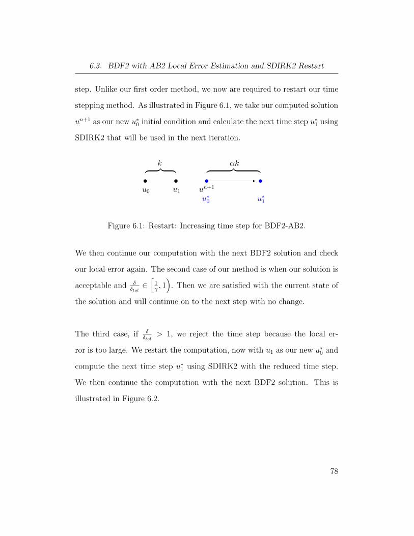
6.3. BDF2 with AB2 Local Error Estimation and SDIRK2 Restart
step. Unlike our first order method, we now are required to restart our time
stepping method. As illustrated in Figure 6.1, we take our computed solution
un+1 as our new u∗0 initial condition and calculate the next time step u∗1 using
SDIRK2 that will be used in the next iteration.
t t t tu0 u1 un+1
u∗0 u∗1
-
︷ ︸︸ ︷k ︷ ︸︸ ︷αk
Figure 6.1: Restart: Increasing time step for BDF2-AB2.
We then continue our computation with the next BDF2 solution and check
our local error again. The second case of our method is when our solution is
acceptable and δδtol∈[
1γ, 1)
. Then we are satisfied with the current state of
the solution and will continue on to the next step with no change.
The third case, if δδtol
> 1, we reject the time step because the local er-
ror is too large. We restart the computation, now with u1 as our new u∗0 and
compute the next time step u∗1 using SDIRK2 with the reduced time step.
We then continue the computation with the next BDF2 solution. This is
illustrated in Figure 6.2.
78

6.3. BDF2 with AB2 Local Error Estimation and SDIRK2 Restart
t ttu0 u1
u∗1u∗0
-
︷ ︸︸ ︷k ︷ ︸︸ ︷k/α
Figure 6.2: Restart: Decreasing time step for BDF2-AB2.
Now we have computed previous time steps for the new time step, and we
continue the iteration. In the case where we have rejected a time step, re-
duced k, and the next time step fails again, we go back and restart again
from the last accepted solution. This requires us to retain the last accepted
solution as a separate variable. The act of rejecting a time step is also used
when our Newton iteration fails to converge, or there are too many CG steps
taken. Tolerances tol its newton and tol its cg are checked during each
Newton iteration. If these counters exceed the given tolerance, we decrease
the time step in the same manner. In practice, we do not see any violation
of our tolerance for Newton iteration.
Our computation continues to increase or decrease the time step through-
out the computation until the time when our given final time is reached.
The last time step is found when our next time step exceeds our user de-
fined end time T . When this occurs, we calculate the last time step using a
SDIRK2 step. We now want to again assess the confidence we have in our
method using the ripening time.
79

6.3. BDF2 with AB2 Local Error Estimation and SDIRK2 Restart
6.3.1 Ripening Time
The ripening time Tr for BDF2-AB2 should be consistent with our BE-FE
solution for us to be confident in both methods. We again compute the
ripening time by looking at the minimum of our current solution. As we let
δtol → 0 we expect our solution to converge to this ripening time as we did
in Chapter 3. We also expect the number of time steps M(δtol) to increase
as δtol is reduced by a factor of 10 by a factor of p+1√
10, where p is the order
of the method, in this case p = 2. Using the same problem for Allen-Cahn
as we did in section 3.11, the results are shown in Table 6.7.
δtol Tr M(δtol)M(δntol)
M(δn−1tol )
1.0000e-04 546.0982 154 2.36921.0000e-05 546.6408 361 2.34421.0000e-06 546.8019 787 2.18011.0000e-07 546.7919 1,696 2.15501.0000e-08 546.7929 3,796 2.23821.0000e-09 546.7970 8,288 2.1834
Table 6.7: Convergence of the ripening time for BDF2-AB2.
We see that our solution converges to Tr = 546.8 which matches our first
order method, and as we expected, the ratio of M(δtol) also converges to
3√
10 = 2.15443. We will use these results to compare to our third order
method. We also see a reduction in required time steps as δtol → 0 compared
to our first order method.
To compare our BDF2-AB2 adaptive method to uniform time steps we carry
80
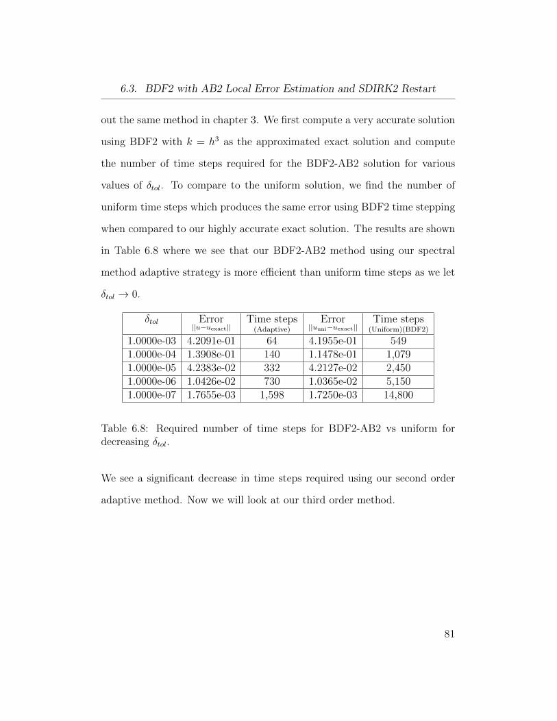
6.3. BDF2 with AB2 Local Error Estimation and SDIRK2 Restart
out the same method in chapter 3. We first compute a very accurate solution
using BDF2 with k = h3 as the approximated exact solution and compute
the number of time steps required for the BDF2-AB2 solution for various
values of δtol. To compare to the uniform solution, we find the number of
uniform time steps which produces the same error using BDF2 time stepping
when compared to our highly accurate exact solution. The results are shown
in Table 6.8 where we see that our BDF2-AB2 method using our spectral
method adaptive strategy is more efficient than uniform time steps as we let
δtol → 0.
δtol Error||u−uexact||
Time steps(Adaptive)
Error||uuni−uexact||
Time steps(Uniform)(BDF2)
1.0000e-03 4.2091e-01 64 4.1955e-01 5491.0000e-04 1.3908e-01 140 1.1478e-01 1,0791.0000e-05 4.2383e-02 332 4.2127e-02 2,4501.0000e-06 1.0426e-02 730 1.0365e-02 5,1501.0000e-07 1.7655e-03 1,598 1.7250e-03 14,800
Table 6.8: Required number of time steps for BDF2-AB2 vs uniform fordecreasing δtol.
We see a significant decrease in time steps required using our second order
adaptive method. Now we will look at our third order method.
81

6.4. BDF3 with AB3 Local Error Estimation and SDIRK3 Restart
6.4 BDF3 with AB3 Local Error Estimation
and SDIRK3 Restart
We consider here a third order scheme similar to the second order scheme
described above. BDF3 time stepping is used with an AB3 predictor and
using an SDIRK3 scheme for restarts.
We now require two initial time steps to start BDF3 initially and three
previous time steps kept throughout the computation. This leads to the
use of SDIRK3 for the initial time steps and restarts. Our BDF3-AB3 time
stepping method follows the same construct as our BDF2-AB2 method. The
local error is now given by
δ =2
5||uBDF3 − uAB3||.
The acceptance of our solution based on this error follows the same method
as our second order method, however now that we have three time steps, we
now do two SDIRK3 steps for each restart as illustrated in Figure 6.3.
t t t t t tu0 u1 u2 un+1
u∗0 u∗1 u∗2
- -
︷ ︸︸ ︷k ︷ ︸︸ ︷αk
Figure 6.3: Restart: Increasing time step for BDF3-AB3.
82
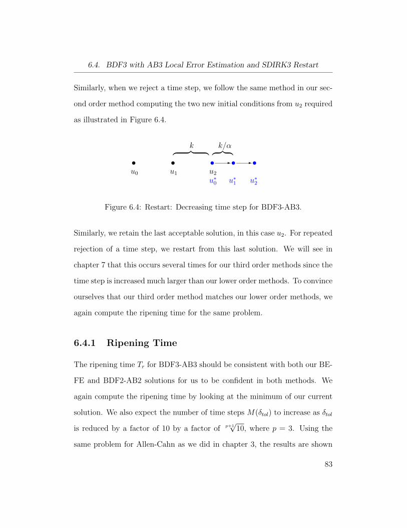
6.4. BDF3 with AB3 Local Error Estimation and SDIRK3 Restart
Similarly, when we reject a time step, we follow the same method in our sec-
ond order method computing the two new initial conditions from u2 required
as illustrated in Figure 6.4.
t t t t tu0 u1 u2
u∗0 u∗1 u∗2
- -
︷ ︸︸ ︷k ︷ ︸︸ ︷k/α
Figure 6.4: Restart: Decreasing time step for BDF3-AB3.
Similarly, we retain the last acceptable solution, in this case u2. For repeated
rejection of a time step, we restart from this last solution. We will see in
chapter 7 that this occurs several times for our third order methods since the
time step is increased much larger than our lower order methods. To convince
ourselves that our third order method matches our lower order methods, we
again compute the ripening time for the same problem.
6.4.1 Ripening Time
The ripening time Tr for BDF3-AB3 should be consistent with both our BE-
FE and BDF2-AB2 solutions for us to be confident in both methods. We
again compute the ripening time by looking at the minimum of our current
solution. We also expect the number of time steps M(δtol) to increase as δtol
is reduced by a factor of 10 by a factor of p+1√
10, where p = 3. Using the
same problem for Allen-Cahn as we did in chapter 3, the results are shown
83

6.4. BDF3 with AB3 Local Error Estimation and SDIRK3 Restart
in Table 6.9.
δtol Tr M(δtol)M(δntol)
M(δn−1tol )
1.0000e-04 546.9734 72 1.35851.0000e-05 546.7535 130 1.80561.0000e-06 546.8286 270 2.07691.0000e-07 546.8152 551 2.04071.0000e-08 546.7992 1,055 1.91471.0000e-09 546.7976 2,087 1.9782
Table 6.9: Convergence of the ripening time for BDF3-AB3 time steppingmethod.
We see that our solution converges to Tr = 546.8 which matches our first
order method in section 3.10 and second order method in section 6.3.1. As
we expected, the ratio of M(δtol) also converges close to 4√
10 = 1.778279. We
have shown that all three methods converge to the same ripening time, which
gives us confidence in these methods of adaptive time stepping. We also see
a reduction in required time steps as δtol → 0 compared to our second order
method.
To compare our BDF3-AB3 adaptive method to uniform time steps we carry
out the same method in section 6.3.1. We use BDF3 time stepping for our
uniform solutions. The results are shown in Table 6.10 where we see that
our BDF3-AB3 method using our spectral method adaptive strategy is more
efficient than uniform time steps as we let δtol → 0.
84
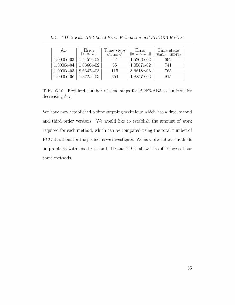
6.4. BDF3 with AB3 Local Error Estimation and SDIRK3 Restart
δtol Error||u−uexact||
Time steps(Adaptive)
Error||uuni−uexact||
Time steps(Uniform)(BDF3)
1.0000e-03 1.5457e-02 47 1.5368e-02 6921.0000e-04 1.0360e-02 65 1.0587e-02 7411.0000e-05 8.6347e-03 115 8.6618e-03 7651.0000e-06 1.8725e-03 254 1.8257e-03 915
Table 6.10: Required number of time steps for BDF3-AB3 vs uniform fordecreasing δtol.
We have now established a time stepping technique which has a first, second
and third order versions. We would like to establish the amount of work
required for each method, which can be compared using the total number of
PCG iterations for the problems we investigate. We now present our methods
on problems with small ε in both 1D and 2D to show the differences of our
three methods.
85
Chapter 7
Numerical Experiments
In this chapter, we focus on the solution to the Allen-Cahn and Cahn-Hilliard
problems with small ε. As we have shown in chapter 3, our adaptive-in-time
strategy is more efficient than uniform time steps in this case. We will now
employ our time stepping methods with spectral discretization and using
PCG to solve for each Newton iteration at each time step. We begin in one
space dimension with the Allen-Cahn equation, where the initial condition
is chosen to be periodic and having the property that only two transitions
from u = ±1 result as the solution progresses. In the case of the Allen-
Cahn equation, this one hump solution will be eventually consumed into one
region of u = 1, while in the Cahn-Hilliard case we consider initial conditions
in which four transition layers appear in early dynamics. Since this model is
volume preserving, the regions of u = −1 cannot disappear but the dynamics
will result in both regions joining together.
86

7.1. Allen-Cahn in 1D
7.1 Allen-Cahn in 1D
For the Allen-Cahn equation in 1D, we apply our method to the same problem
in chapter 3, but now with ε = 0.12. We compute the solution for all three
methods to show how our second and third order methods perform versus
our first order method. In this problem however, the time scale is very large,
with T = 31, 055. Our initial condition is again u0(x) = sinx+0.8 on [0, 2π].
The parameters we have chosen are
ε = 0.12, n = 128,
T = 31, 055, tol delta = 10−4,
θ = 0.8, tol newton = 10−8,
γ = 3, tol cg = 10−9.
.
What we observe is three phases in the solution. A fast transition from the
initial condition to the metastable state. We then experience a long time
scale in this state, and then eventually we pass the ripening time, which
again is fast as the solution arrives at stable state of u = +1. The behaviour
where the activity between phases is confined to the start and end of the
computation with a long metastable state can be seen in Figure 7.1.
87

7.1. Allen-Cahn in 1D
Figure 7.1: Space-Time plot for Allen-Cahn in 1D for ε = 0.12, γ = 3 for theBDF3-AB3 method.
In this figure we show the BDF3-AB3 solution that exhibits large time steps
during the metastable state, seen by increasing distance of grid lines, and a
similar situation occurs with our BE-FE and BDF2-AB2 methods. This is
seen more clearly in Figure 7.2.
Figure 7.2: Evolution of time step k vs. t for Allen-Cahn in 1D for ε =0.12, γ = 3.
88
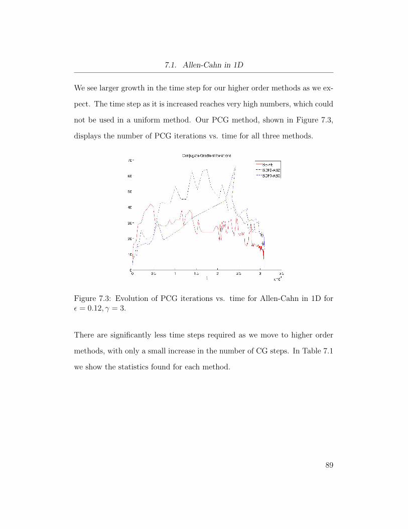
7.1. Allen-Cahn in 1D
We see larger growth in the time step for our higher order methods as we ex-
pect. The time step as it is increased reaches very high numbers, which could
not be used in a uniform method. Our PCG method, shown in Figure 7.3,
displays the number of PCG iterations vs. time for all three methods.
Figure 7.3: Evolution of PCG iterations vs. time for Allen-Cahn in 1D forε = 0.12, γ = 3.
There are significantly less time steps required as we move to higher order
methods, with only a small increase in the number of CG steps. In Table 7.1
we show the statistics found for each method.
89
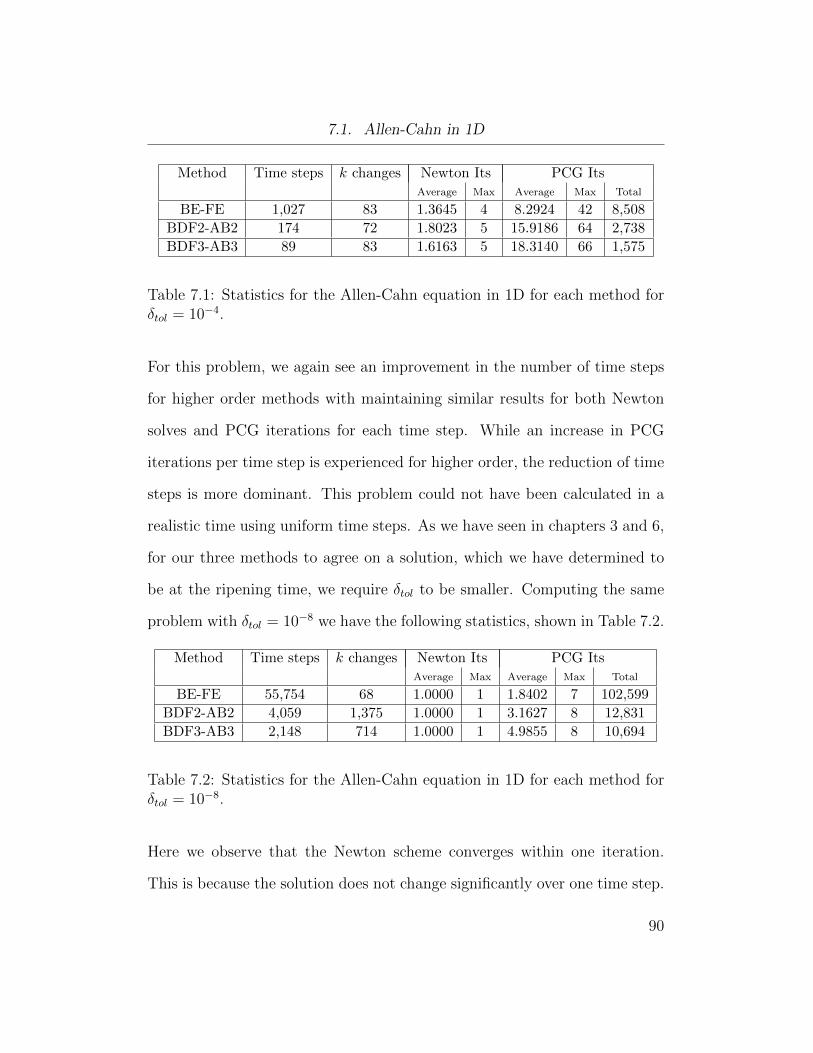
7.1. Allen-Cahn in 1D
Method Time steps k changes Newton Its PCG ItsAverage Max Average Max Total
BE-FE 1,027 83 1.3645 4 8.2924 42 8,508
BDF2-AB2 174 72 1.8023 5 15.9186 64 2,738
BDF3-AB3 89 83 1.6163 5 18.3140 66 1,575
Table 7.1: Statistics for the Allen-Cahn equation in 1D for each method forδtol = 10−4.
For this problem, we again see an improvement in the number of time steps
for higher order methods with maintaining similar results for both Newton
solves and PCG iterations for each time step. While an increase in PCG
iterations per time step is experienced for higher order, the reduction of time
steps is more dominant. This problem could not have been calculated in a
realistic time using uniform time steps. As we have seen in chapters 3 and 6,
for our three methods to agree on a solution, which we have determined to
be at the ripening time, we require δtol to be smaller. Computing the same
problem with δtol = 10−8 we have the following statistics, shown in Table 7.2.
Method Time steps k changes Newton Its PCG ItsAverage Max Average Max Total
BE-FE 55,754 68 1.0000 1 1.8402 7 102,599
BDF2-AB2 4,059 1,375 1.0000 1 3.1627 8 12,831
BDF3-AB3 2,148 714 1.0000 1 4.9855 8 10,694
Table 7.2: Statistics for the Allen-Cahn equation in 1D for each method forδtol = 10−8.
Here we observe that the Newton scheme converges within one iteration.
This is because the solution does not change significantly over one time step.
90
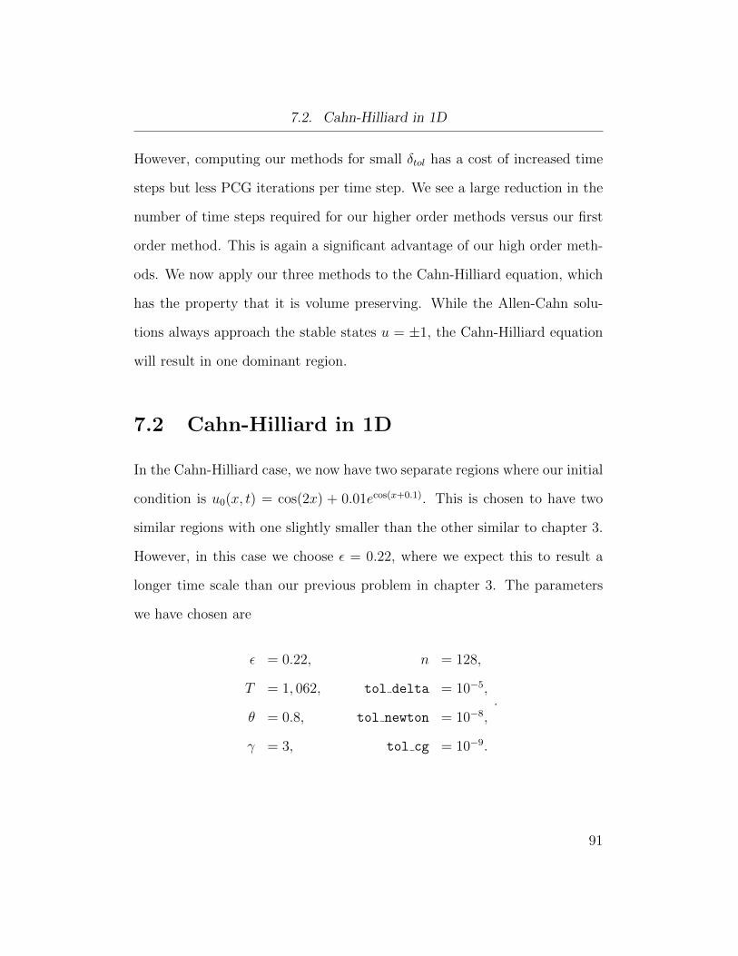
7.2. Cahn-Hilliard in 1D
However, computing our methods for small δtol has a cost of increased time
steps but less PCG iterations per time step. We see a large reduction in the
number of time steps required for our higher order methods versus our first
order method. This is again a significant advantage of our high order meth-
ods. We now apply our three methods to the Cahn-Hilliard equation, which
has the property that it is volume preserving. While the Allen-Cahn solu-
tions always approach the stable states u = ±1, the Cahn-Hilliard equation
will result in one dominant region.
7.2 Cahn-Hilliard in 1D
In the Cahn-Hilliard case, we now have two separate regions where our initial
condition is u0(x, t) = cos(2x) + 0.01ecos(x+0.1). This is chosen to have two
similar regions with one slightly smaller than the other similar to chapter 3.
However, in this case we choose ε = 0.22, where we expect this to result a
longer time scale than our previous problem in chapter 3. The parameters
we have chosen are
ε = 0.22, n = 128,
T = 1, 062, tol delta = 10−5,
θ = 0.8, tol newton = 10−8,
γ = 3, tol cg = 10−9.
.
91

7.2. Cahn-Hilliard in 1D
Similarly to Allen-Cahn, in early dynamics the solution tends to u = ±1 in
regions with transition layers of width O(ε) between them. This metastable
state evolves slowly in time as the center between the two u = −1 regions will
eventually decrease in size and becomes absorbed. This type of dynamic can
be explained as exponential tails for each region interacting with each other
[5]. We observe the entire solution in a space-time plot shown in Figure 7.4.
Figure 7.4: Space-Time plot for the Cahn-Hillard in 1D for ε = 0.22, γ = 3with the BDF3-AB3 Method.
Figure 7.4 is situated with the end in front to show that indeed both regions
were absorbed into one. Similar to the Allen-Cahn model in the previous sec-
tion, the evolution of the time step has the same type of peak from increasing
to decreasing as we pass through the metastable state, shown in Figure 7.5.
92
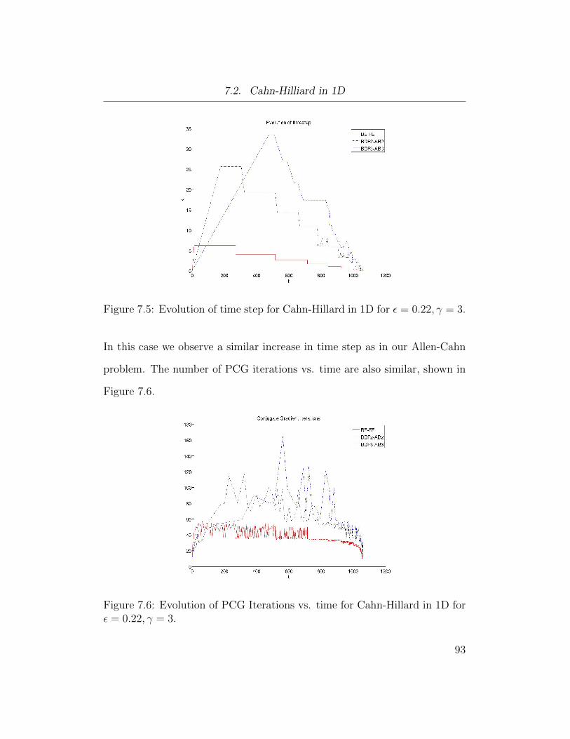
7.2. Cahn-Hilliard in 1D
Figure 7.5: Evolution of time step for Cahn-Hillard in 1D for ε = 0.22, γ = 3.
In this case we observe a similar increase in time step as in our Allen-Cahn
problem. The number of PCG iterations vs. time are also similar, shown in
Figure 7.6.
Figure 7.6: Evolution of PCG Iterations vs. time for Cahn-Hillard in 1D forε = 0.22, γ = 3.
93
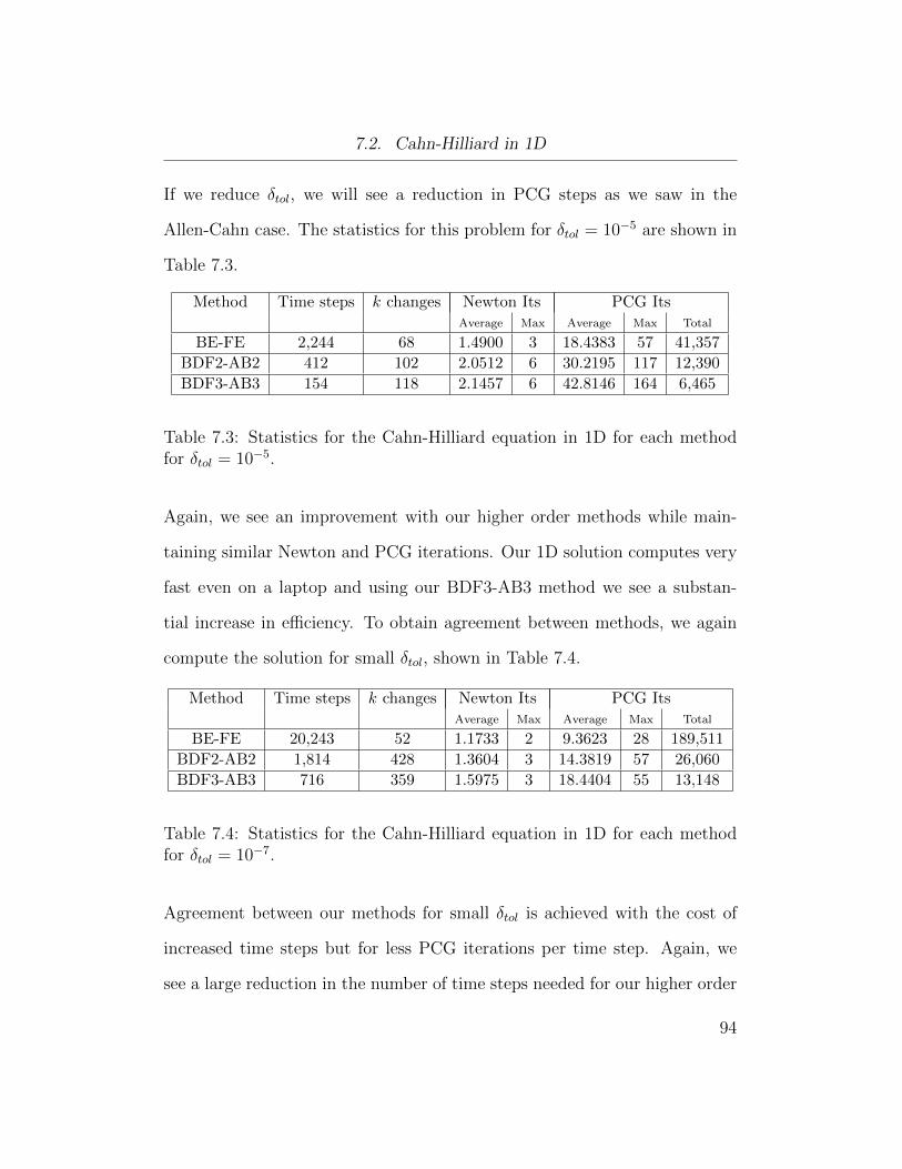
7.2. Cahn-Hilliard in 1D
If we reduce δtol, we will see a reduction in PCG steps as we saw in the
Allen-Cahn case. The statistics for this problem for δtol = 10−5 are shown in
Table 7.3.
Method Time steps k changes Newton Its PCG ItsAverage Max Average Max Total
BE-FE 2,244 68 1.4900 3 18.4383 57 41,357
BDF2-AB2 412 102 2.0512 6 30.2195 117 12,390
BDF3-AB3 154 118 2.1457 6 42.8146 164 6,465
Table 7.3: Statistics for the Cahn-Hilliard equation in 1D for each methodfor δtol = 10−5.
Again, we see an improvement with our higher order methods while main-
taining similar Newton and PCG iterations. Our 1D solution computes very
fast even on a laptop and using our BDF3-AB3 method we see a substan-
tial increase in efficiency. To obtain agreement between methods, we again
compute the solution for small δtol, shown in Table 7.4.
Method Time steps k changes Newton Its PCG ItsAverage Max Average Max Total
BE-FE 20,243 52 1.1733 2 9.3623 28 189,511
BDF2-AB2 1,814 428 1.3604 3 14.3819 57 26,060
BDF3-AB3 716 359 1.5975 3 18.4404 55 13,148
Table 7.4: Statistics for the Cahn-Hilliard equation in 1D for each methodfor δtol = 10−7.
Agreement between our methods for small δtol is achieved with the cost of
increased time steps but for less PCG iterations per time step. Again, we
see a large reduction in the number of time steps needed for our higher order
94
7.3. Allen-Cahn in 2D
methods versus our first order method. We now present problems in 2D for
both the Allen-Cahn and Cahn-Hilliard equations.
7.3 Allen-Cahn in 2D
In two space dimensions, we now have the domain Ω = [0, 2π]2, and our
methods are easily extended to this case. Our discretization is now
Un+1 − Un
k= ε2DUn+1 + w′(Un+1),
where U is a matrix corresponding to each mesh point in the domain. The
matrix D is now the spectral approximation of the 2D Laplacian. The only
difference from the method that we have been using in one space dimension
is the mesh and the Liapunov energy. In our spectral method, we also use
the 2D version of the FFT. We consider the initial condition u0(x, y, t) =
2e(sinx+sin y−2) + 2.2e(− sinx−sin y−2) − 1. The parameters we have chosen are
ε = 0.18, n = 64,
T = 33, tol delta = 10−5,
θ = 0.8, tol newton = 10−8,
γ = 3, tol cg = 10−9.
.
We choose ε = 0.18, and we expect that the smaller region will be annihilated
first followed by the second larger region which occurs at T = 33. This is
95
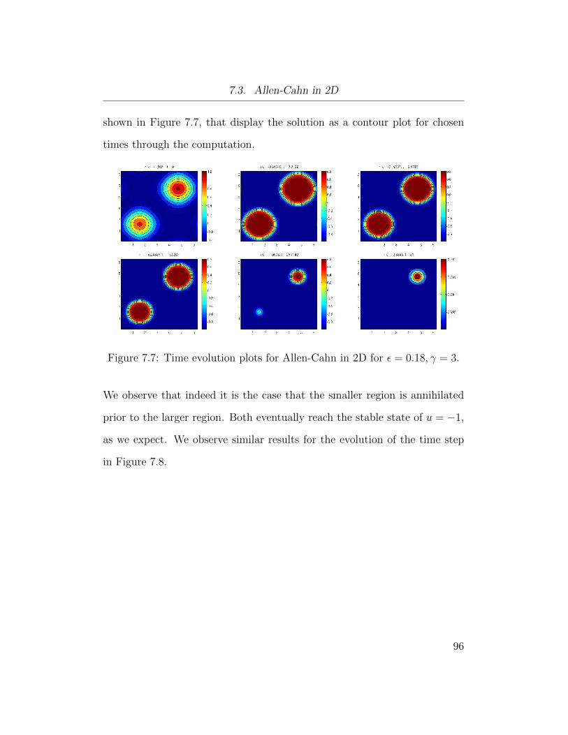
7.3. Allen-Cahn in 2D
shown in Figure 7.7, that display the solution as a contour plot for chosen
times through the computation.
Figure 7.7: Time evolution plots for Allen-Cahn in 2D for ε = 0.18, γ = 3.
We observe that indeed it is the case that the smaller region is annihilated
prior to the larger region. Both eventually reach the stable state of u = −1,
as we expect. We observe similar results for the evolution of the time step
in Figure 7.8.
96

7.3. Allen-Cahn in 2D
Figure 7.8: Evolution of time step for Allen-Cahn in 2D for ε = 0.18, γ = 3.
Again, this problem is also difficult to solve using uniform time steps. Our
higher order methods increase the time step rapidly and require far less than
we would with a uniform method. The number of PCG iterations required
is shown in Figure 7.9.
97

7.3. Allen-Cahn in 2D
Figure 7.9: Evolution of PCG iterations vs. time for Allen-Cahn in 2D forε = 0.18, γ = 3.
While we see an increase in PCG steps for our higher order methods, in
Table 7.5 we present statistics for δtol = 10−4.
Method Time steps k changes Newton Its PCG ItsAverage Max Average Max Total
BE-FE 2,970 28 1.0000 1 2.6639 4 7,909
BDF2-AB2 492 48 1.0000 1 4.2898 7 2,102
BDF3-AB3 175 52 1.0000 1 5.4302 8 934
Table 7.5: Statistics for the Allen-Cahn equation in 2D for each method forδtol = 10−4.
Again, we see a substantial improvement with our higher order methods. To
obtain agreement between methods, we again compute the solution for small
δtol, shown in Table 7.6.
98

7.4. Cahn-Hilliard in 2D
Method Time steps k changes Newton Its PCG ItsAverage Max Average Max Total
BE-FE 29,099 25 1.0000 1 1.0000 1 29,098
BDF2-AB2 2,384 41 1.0000 1 1.6495 3 3,929
BDF3-AB3 699 51 1.0000 1 2.2773 4 1,585
Table 7.6: Statistics for the Allen-Cahn equation in 2D for each method forδtol = 10−7.
For 2D, we see that our higher order methods are far more efficient than first
order.
7.4 Cahn-Hilliard in 2D
Using the same initial condition as in the Allen-Cahn equation, now with
T = 81, the parameters we have chosen are
ε = 0.18, n = 128,
T = 81, tol delta = 10−3,
θ = 0.9, tol newton = 10−7,
γ = 2, tol cg = 10−8.
.
We show the evolution of the solution for the Cahn-Hilliard problem in 2D
in Figure 7.10.
99
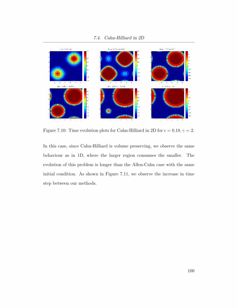
7.4. Cahn-Hilliard in 2D
Figure 7.10: Time evolution plots for Cahn-Hilliard in 2D for ε = 0.18, γ = 2.
In this case, since Cahn-Hilliard is volume preserving, we observe the same
behaviour as in 1D, where the larger region consumes the smaller. The
evolution of this problem is longer than the Allen-Cahn case with the same
initial condition. As shown in Figure 7.11, we observe the increase in time
step between our methods.
100
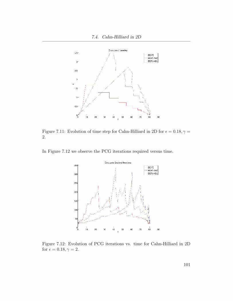
7.4. Cahn-Hilliard in 2D
Figure 7.11: Evolution of time step for Cahn-Hilliard in 2D for ε = 0.18, γ =2.
In Figure 7.12 we observe the PCG iterations required versus time.
Figure 7.12: Evolution of PCG iterations vs. time for Cahn-Hilliard in 2Dfor ε = 0.18, γ = 2.
101

7.4. Cahn-Hilliard in 2D
In Table 7.7 we again see the improvement our higher order methods have
on the the number of time steps required to compute the solution.
Method Time steps k changes Newton Its PCG ItsAverage Max Average Max Total
BE-FE 380 77 2.4617 5 44.9763 248 17,046
BDF2-AB2 125 102 2.6667 8 70.7642 338 8,704
BDF3-AB3 90 99 2.2414 7 73.0920 307 6,359
Table 7.7: Statistics for the Cahn-Hilliard equation in 2D for each methodfor δtol = 10−3.
Again, to obtain agreement between methods, we again compute the solution
for small δtol, shown in Table 7.8, we we see our most improvement in the
problems presented.
Method Time steps k changes Newton Its PCG ItsAverage Max Average Max Total
BE-FE 11,162 69 1.1992 2 9.8847 22 110,323
BDF2-AB2 1,309 461 1.3940 2 17.2510 34 22,547
BDF3-AB3 516 274 1.6589 2 22.7018 40 11,646
Table 7.8: Statistics for the Cahn-Hilliard equation in 2D for each methodfor δtol = 10−7.
The problems presented here show cases where adaptive time stepping meth-
ods are far superior to uniform methods. In addition, we have shown the
efficiency gains of using higher order BDF time stepping methods. For very
small ε, we have shown that these problems exhibit behaviour that can only
be calculated in this manner, and we have increased efficiency while not los-
ing accuracy. We have also shown that as we request more accuracy through
102

7.4. Cahn-Hilliard in 2D
δtol, we have a relationship between an increase of time steps and a decrease
in PCG steps. The code for these problems can be easily extended to other
problems of this type, such as higher order or vector gradient flows coming
from material science models.
103

Chapter 8
Conclusions and Future Work
We have presented a numerical method for solving the Allen-Cahn and Cahn-
Hilliard equations as it relates to material science. Steep transition layers
between materials that we see in applications such as annealing, can be re-
solved and a fast and efficient solution is found using adaptive time stepping
techniques. The method presented addresses the challenges in a numerical
solution for these problems and offers increased efficiency and the ability to
compute problems can can not be solved using traditional methods.
Using asymptotic analysis, we have shown that we expect the transition
layers to behave as a tanh function between u = ±1, with width O(ε) as
they move slowly in time. To build a numerical model, we first develop the
first order Forward Euler explicit scheme as our predictor and the Backward
Euler implicit scheme as our corrector. For our discretization in space we
use standard finite difference methods. What results is a nonlinear system
of equations to solve for each time step, and we employ Newton iteration
to solve this system. Our adaptive strategy is to use the difference between
the predictor and corrector as the local error δ. Once δ is within a preset
104
Chapter 8. Conclusions and Future Work
tolerance, the time step k is then increased. We increase the time step by a
factor of ξ, or decrease by a factor of 1/ξ, for preset values given by the user.
The parameter ξ is set up so that our increase will not violate our tolerances
for the local error in the next time step. This method is applied to a problem
that presents challenges for a uniform method and we show that it is indeed
more efficient than the uniform method.
We then utilize spectral methods for the spatial discretization that make the
spatial error negligible for a sufficient number of grid points I, and presents
a substantial increase in efficiency. We now solve for each Newton iteration
using preconditioned conjugate gradient method, where we have developed a
linear model preconditioner. It is a constant coefficient version of the system,
suggested to us by Scott MacLachlan. The preconditioner for this problem
is one of the major contributions of this work. The preconditioner reduces
the CG iterations by a significant factor and can be implemented efficiently
using the fast Fourier transform.
As the Backward Euler method is a first order time stepping technique,
it is natural to consider second and third order methods. Using backward
difference formulas of second and third order, coupled with Adams Bashforth
methods as our predictor of the same orders, we show that these methods are
even more efficient than our first order model. In our numerical experiments,
we show that our third order method is the most efficient.
105
8.1. Future Work
There are many applications of the Allen-Cahn and Cahn-Hilliard equations,
with higher order and vector relatives of these equations where our method
can be applied. It is our intention to present code that can be easily exten-
sible to these other problems.
8.1 Future Work
While we have shown the power of adaptivity in time for 1D and 2D, for large
3D problems such as cancerous tumor growth the domain may be largely one
material and relying on a uniform spatial grid to calculate the solution may
no longer be feasible. The computation, as was presented in [15], can be
greatly improved with adaptivity in space and time. Since the most activity
that occurs during the computation is in the transition layer, it is natural to
include more grid points in this area, while less grid points are required far
away from the transition layer. In future work, we plan to consider spatially
adaptive discretization coupled with multigrid solvers.
There are three general approaches to compute a solution with a non-uniform
grid. Consider the layered grid in Figure 8.1.
106
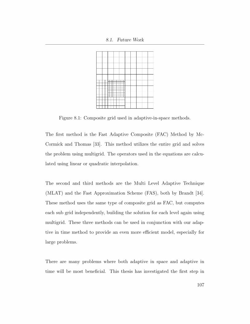
8.1. Future Work
Figure 8.1: Composite grid used in adaptive-in-space methods.
The first method is the Fast Adaptive Composite (FAC) Method by Mc-
Cormick and Thomas [33]. This method utilizes the entire grid and solves
the problem using multigrid. The operators used in the equations are calcu-
lated using linear or quadratic interpolation.
The second and third methods are the Multi Level Adaptive Technique
(MLAT) and the Fast Approximation Scheme (FAS), both by Brandt [34].
These method uses the same type of composite grid as FAC, but computes
each sub grid independently, building the solution for each level again using
multigrid. These three methods can be used in conjunction with our adap-
tive in time method to provide an even more efficient model, especially for
large problems.
There are many problems where both adaptive in space and adaptive in
time will be most beneficial. This thesis has investigated the first step in
107

8.1. Future Work
this direction, where we find that a substantial increase in efficiency can be
found in adaptive-in-time methods.
We are also interested in more efficient use of CG, such as variable toler-
ances depending on the performance of the Newton scheme. Since there are
a relatively small number of Newton steps in our problems for each time step,
it may be beneficial to explore these avenues to gain more efficiency.
108
Bibliography
[1] S.M. Allen and J.W. Cahn. A microscopic theory for antiphase boundary
motion and its application to antiphase domain coarsening. Acta Metall.
Mater. 27 (1979), 1085-1095.
[2] J.W. Cahn and J.E. Hilliard. Free energy of a nonuniform system. I.
interfacial free energy. J. Chem. Phys. 28 (1958), 258-267.
[3] L. Bronsard, D. Hilhorst. On the slow dynamics for the Cahn-Hilliard
equation in one space dimension. Proceedings: Mathematical and Phys-
ical Sciences 439, 1907 (1992), 669-682.
[4] J. Shen, X. Yang. Numerical approximations of Allen-Cahn and Cahn-
Hilliard equations [Preprint]
[5] M. Ward. Metastable bubble solutions for the Allen-Cahn equation with
mass conservation. SIAM Journal on Applied Mathematics 56, 5 (1996).
[6] C. Grantt and E. Vleckts. Slowly-migrating transition layers for the
discrete Allen-Cahn and Cahn-Hilliard equations. Nonlinearity 8 (1995),
861.
109
Bibliography
[7] P. Bates, S. Brown, J. Han, Numerical analysis for a nonlocal Allen-
Cahn equation, Numerical Analysis and Modeling 6, 1 (2009), 33-49.
[8] J.D. Verhoeven, Fundamentals of Physical Metallurgy, (1975) Wiley,
New York.
[9] E. V. L. de Mello, O. T. S. Filho, Numerical study of the Cahn-Hilliard
equation in one, two and three dimensions, Physica A 347 (2005), 429-
443.
[10] S. A. Orszag, Numerical methods for the simulation of turbulence, Phys.
Fluids Supp. II, 12 (1969) 250-257
[11] MacLachlan, S. (Tufts University), Personal Communication, October
5, 2010
[12] L. Trefethen, Spectral Methods in MATLAB, (2000) Society for Indus-
trial and Applied Mathematics.
[13] Canuto, C. et. al., Spectral Methods in Fluid Dynamics, (1988) Springer-
Verlag.
[14] K. Promislow, B. Wetton, PEM fuel cells: a mathematical overview.
Siam J. Appl. Math 70, 2 (2009), 359-409.
[15] S.M. Wise, J.S. Lowengrub, V. Cristini, An adaptive multigrid algorithm
for simulating solid tumor growth using mixture models, Mathematical
and Computer Modelling 53 (2011), 120.
110
Bibliography
[16] P.W. Bates, E.N. Dancer, J. Shi, Multi-spike stationary solutions of the
Cahn-Hilliard equation in higher-dimension and instability, Advances in
Diff. Eqts. 4 (1999), 1-69.
[17] P. Howard, Asymptotic behavior near planar transition fronts for the
Cahn-Hilliard equation, Physica D: Nonlinear Phenomena 229, 2 (2007)
123-165.
[18] A. Novick-Cohen, Triple-junction motion for an Allen-Cahn/Cahn-
Hilliard system, Physica D: Nonlinear Phenomena 137, 1-2 (2000) 1-24.
[19] S. Liu, F. Wang, H. Zhao, Global existence and asymptotics of solutions
of the CahnHilliard equation, Journal of Differential Equations 238, 2
(2007) 426-469.
[20] K.W. Morton, D.F. Mayers, Numerical Solution of Partial Differential
Equations, (2005) Cambridge University Press.
[21] Euler, L. Institutiones Calculi Integralis (1768)
[22] S. Minkoff, N. Kridler. A comparison of adaptive time stepping meth-
ods for coupled flow and deformation modeling. Applied Mathematical
Modelling (2005).
[23] Y. Saad, Iterative Methods for Sparse Linear Systems, (2003) Society
for Industrial and Applied Mathematics.
[24] J. Demmel, Applied Numerical Linear Algebra, (1997) SIAM.
111
Bibliography
[25] L. Trefethen, D. Bau, Numerical Linear Algebra, (1997) SIAM.
[26] U. Ascher, C. Grief, A First Course on Numerical Methods, (2011) So-
ciety for Industrial and Applied.
[27] J. R. Higgins, Five Short Stories About The Cardinal Series, Bull. Amer.
Math. Soc. 12 (1985), 45-89.
[28] E. Hairer, S.P. Nørsett, G. Wanner. Solving Ordinary Differential Equa-
tions I - Nonstiff Problems. (1993) Springer-Verlag Berlin Heidelberg
[29] E. Hairer, S.P. Nørsett, G. Wanner. Solving Ordinary Differential Equa-
tions II - Stiff and Differential-Algebraic Problems. (1991) Springer-
Verlag Berlin Heidelberg
[30] P. Gresho, D. Griffiths, D. Silvester. Adaptive time-stepping for incom-
pressible flow part I: scalar advection-diffusion. SIAM J. Sci. Comput.
30, 4 (2008), 2018-2054.
[31] J. Evans, Course notes for mathematical modelling and industrial math-
ematics, University of Bath.
[32] Fasshauer, G. E. Newton iteration with multiquadrics for the solution
of nonlinear PDEs. Journal of Computers and Mathematics with Appli-
cations, 43 (2002), 423-438.
112
Bibliography
[33] S. McCormick, J. Thomas, The fast adaptive composite grid (FAC)
method for elliptic equations. Mathematics of Computation, 46:174
(1986) 439-456
[34] A. Brandt, Multi-level adaptive technique (MLAT) for fast numerical
solution to boundary value problems. (1973)
113