high frame rate ultrasound imaging using parallel beamforming
TRANSCRIPT
High frame rate ultrasound imaging using parallelbeamforming
Thesis for the degree of Philosophiae Doctor
Trondheim, January 2009
Norwegian University of Science and TechnologyFaculty of MedicineDepartment of Circulation and Medical Imaging
Tore Grüner Bjåstad

NTNUNorwegian University of Science and Technology
Thesis for the degree of Philosophiae Doctor
Faculty of MedicineDepartment of Circulation and Medical Imaging
© Tore Grüner Bjåstad
ISBN 978-82-471-1405-6 (printed ver.)ISBN 978-82-471-1406-3 (electronic ver.)ISSN 1503-8181
Doctoral theses at NTNU, 2009:18
Printed by NTNU-trykk

Høg bilderate i ultralydavbilding ved hjelp av parallell straleforming
Denne avhandlinga omhandlar ein teknikk for a auke ultralyd bilderate kalla parallellstraleforming. Bruksomradet er avgrensa til hjerteavbilding, sidan det er denne typeavbilding som stiller høgast krav til bilderate.
Hjartemuskelen trekk seg saman og slappar av omtrent ein gong kvart sekund.Kontraksjonen er ein kompleks prosess der ulike delar av hjartet trekk seg samantil ulike tider og med forskjellig hastigheit. For a kunne studere denne bevegelsennøyaktig med ultralyd, treng ein høg bilderate. Eit ultralydbilete vert danna ved askyte ein avbildingspuls langs ei rekke med skannelinjer som dekker objektet ein vilavbilde. Bilderata er da begrensa av kor mange stralar ein nyttar, og av tida det tarfor ein avbildingspuls a propagere langs ei skannelinje til maksimal avbildingsdybdeog attende.
Multippel linjeakkvisisjon, MLA, er ein teknikk som ofte vert nytta for a aukebilderata. I staden for a lage kun ei bildelinje for kvar sendepuls, lagar ein med denneteknikken fleire linjer i parallell. Teknikken vert ogsa kalla parallell straleforming ogkan da auke bilderata proporsjonalt med antalet parallelle skannelinjer. Ulempa medteknikken er at den fører til uønska bildeartefakt. Artefakta har ein stripeliknandesutsjanad og er spesielt tydelige i bildesekvensar (filmar). Eit mal med denneavhandlinga er a kunne nytte parallell straleforming til a auke bilderata utan at detresulterar i bildeartefakt.
Avhandlinga inneheld resultat fra data-simuleringar, in-vitro- og in-vivo malingar.Det visast at forskyvinga mellom sende- og mottakarretning nar ein nyttar MLAfordreiar puls-ekko-responsen til kvar skannelinje. Dette gir eit skift-variantavbildingssystem med bildeartefakt. Avhandlinga omfattar fire bidrag. Bidragainneheld beskrivingar av malemetodar for a evaluere og kvantifisere puls-ekko-fordreiinga, bildeartefakt og skiftinvarians. Bidraga inneheld ogsa evalueringar ogsamanlikningar av forskjellige metodar for reduksjon av MLA-bildeartefakt. Deito metodane som har blitt mest vektlagt er styringskompensasjon og syntetiskesendestralar (STB, Synthetic Transmit Beam). Styringskompensasjon gav godreduksjon av bildeartefakt under ideelle forhold, men virkninga vart kraftig reduserti realistiske scenario med aberrasjonar. STB-metoda metoda gav god reduksjon avbildeartefakt bade med og utan aberrasjonar. I tillegg visast det at ein ved a nytteSTB akvisisjonsmønsteret ogsa kan estimere vevshastigheit med ei nøyaktigheit somer samanliknbar med konvensjonell vevsdoppler.
Tore Gruner BjastadInstitutt for sirkulasjon og bildediagnostikk, NTNUHovedveileder: Hans Torp, Biveileder: Kjell Kristoffersen
Ovennevnte avhandling er funnet verdig til a forsvares offentlig for graden philosophiaedoctor (PhD) i medisinsk teknologi. Disputas finner sted i auditoriet, Øya Helsehus,fredag 30. januar kl. 12:15.

Abstract
The human heart contracts and relaxes approximately once each second. This isa complex process where different parts of the cardiac tissue contract and relax atdifferent times and at different rates. The accurate evaluation of this deformation withultrasound requires the use of a high frame rate. The frame rate of a conventionalultrasound image is limited by the round trip propagation time of the sound pulse alongeach of the scan lines covering the imaged object. A common technique to increase theframe rate is multiple line acquisition, MLA. Using this technique, several scan linesare acquired in parallel for each transmitted pulse. This technique is therefore alsocalled parallel beamforming. Although it increases the frame rate in proportion tothe number of parallel beams, this technique also introduces block-like artifacts in theB-mode image. These artifacts severely degrade the image quality, and are especiallyvisible in image sequences (movies). An aim of this thesis is to investigate methodsto increase the frame rate using parallel beamforming without introducing such imageartifacts.
Investigations of the mechanisms of MLA image artifacts have shown that themisalignment of the transmit and receive beams causes distortions to the pulse-echoresponses. These distortions result in a shift variant imaging system and imageartifacts. This thesis is comprised of four papers that document several metrics thathave been developed to evaluate the pulse-echo distortions, image artifacts and shiftinvariance property. Different methods for artifact reduction have been compared andevaluated. The two methods that have been most thoroughly investigated are steeringcompensation and the synthetic transmit beam method, STB. In the first method, thereceive beams are additionally steered to partially avoid the pulse-echo distortion.Applying this method reduced image artifacts under ideal conditions. However,the performance was heavily reduced in realistic scenarios with aberrations. In theSTB method, synthetic transmit beams are created in each receive direction throughinterpolation. This method performed well both with and without aberrations.Additionally, it has been shown that from the same STB acquisition pattern it is alsopossible to estimate velocities with an accuracy comparable to that of conventionalTDI. This enables higher TDI frame rates or a larger field of view compared toconventional TDI, which requires separate acquisitions for B-mode and tissue Doppler.

Preface
The present thesis is submitted in partial fulfillment of the requirements for thedegree of PhD at the Faculty of Medicine at the Norwegian University of Scienceand Technology (NTNU). The research was funded by NTNU, and was carried outunder the supervision of Professor Hans Torp in the Department of Circulation andMedical Imaging, NTNU.
Acknowledgments
Several people have been involved in the work presented in this thesis and deservemy gratitude. First of all I would like to thank my supervisor, Professor Hans Torp.His support and guidance throughout this work has been invaluable. He has beenavailable for assistance 24 hours a day, 365 days a year during my time here. Throughhis profound knowledge of ultrasound, he has always been able to find solutions orgood approaches to solve my problems (preferably via a quick K-space analysis of it).
I would also like to thank my colleagues and co-authors Torbjørn Hergum andSvein Arne Aase. Torbjørn had a head start on the STB technique in the autumn of2003. I joined in during the spring of 2004 as the co-author on the first article on STB.Discussions then and later have been of great importance for my work. Svein Arne hasbeen my roommate during the last few years and co-author on my second and thirdpaper. His efficiency and companionship has been very valuable both for my academicwork and for enjoyable days at the office. I further would like to thank all my othercolleagues and fellow PhD students in the department. Your social companionship andour technical discussions have made the days at the department fun and inspiring.
I would also like to express my gratitude to the people at GE Vingmed for their helpand support with hardware and software. A special thanks goes to my co-supervisor,Kjell Kristoffersen. His broad technical knowledge has been of great help to mywork. The Trondheim ultrasound group works in close collaboration with clinicians;through this collaboration I have been given help on clinical issues and have acquiredprofessionally scanned ultrasound images. This has been greatly appreciated.
Finally I would like to thank my dear wife, Karianne, for her encouragement,understanding and love throughout these years.


Table of Contents
1 Introduction 131.1 Ultrasound data acquisition . . . . . . . . . . . . . . . . . . . . . . . . 14
1.1.1 Scanning modes . . . . . . . . . . . . . . . . . . . . . . . . . . 141.1.2 Ultrasound transducer . . . . . . . . . . . . . . . . . . . . . . . 151.1.3 Probe types . . . . . . . . . . . . . . . . . . . . . . . . . . . . . 161.1.4 Basic beamforming . . . . . . . . . . . . . . . . . . . . . . . . . 171.1.5 Beam profiles . . . . . . . . . . . . . . . . . . . . . . . . . . . . 181.1.6 Common beamforming techniques . . . . . . . . . . . . . . . . 201.1.7 Image Quality . . . . . . . . . . . . . . . . . . . . . . . . . . . 211.1.8 Shift invariance . . . . . . . . . . . . . . . . . . . . . . . . . . . 241.1.9 Body wall distortion effects . . . . . . . . . . . . . . . . . . . . 241.1.10 Biomechanical effects of ultrasound . . . . . . . . . . . . . . . . 241.1.11 Sampling . . . . . . . . . . . . . . . . . . . . . . . . . . . . . . 25
1.2 Frame Rate . . . . . . . . . . . . . . . . . . . . . . . . . . . . . . . . . 261.2.1 IQ interpolation . . . . . . . . . . . . . . . . . . . . . . . . . . 271.2.2 Multiple Line Acquisition, MLA . . . . . . . . . . . . . . . . . 281.2.3 Multiple Line Transmission, MLT . . . . . . . . . . . . . . . . . 291.2.4 Synthetic Aperture . . . . . . . . . . . . . . . . . . . . . . . . . 311.2.5 High frame rate using limited diffraction beams . . . . . . . . . 32
1.3 MLA artifacts . . . . . . . . . . . . . . . . . . . . . . . . . . . . . . . . 331.4 Tissue Doppler Imaging . . . . . . . . . . . . . . . . . . . . . . . . . . 351.5 Motivation and aims of study . . . . . . . . . . . . . . . . . . . . . . . 371.6 Summary of presented work . . . . . . . . . . . . . . . . . . . . . . . . 371.7 Discussion . . . . . . . . . . . . . . . . . . . . . . . . . . . . . . . . . . 401.8 Conclusion . . . . . . . . . . . . . . . . . . . . . . . . . . . . . . . . . 421.9 Publication list . . . . . . . . . . . . . . . . . . . . . . . . . . . . . . . 43References . . . . . . . . . . . . . . . . . . . . . . . . . . . . . . . . . . . . . 44
2 Parallel Beamforming using Synthetic Transmit Beams 492.1 Introduction . . . . . . . . . . . . . . . . . . . . . . . . . . . . . . . . . 502.2 Background and Problem Statement . . . . . . . . . . . . . . . . . . . 502.3 Shift Invariance through Coherent Interpolation . . . . . . . . . . . . . 532.4 Compensation Methods . . . . . . . . . . . . . . . . . . . . . . . . . . 56
9

Table of Contents
2.4.1 Synthetic Transmit Beams . . . . . . . . . . . . . . . . . . . . . 562.4.2 Dynamic steering . . . . . . . . . . . . . . . . . . . . . . . . . . 572.4.3 US patent by J. N. Wright . . . . . . . . . . . . . . . . . . . . 582.4.4 Simulation- and experimental setup . . . . . . . . . . . . . . . 58
2.5 Results and Discussion . . . . . . . . . . . . . . . . . . . . . . . . . . . 582.6 Concluding Remarks . . . . . . . . . . . . . . . . . . . . . . . . . . . . 66References . . . . . . . . . . . . . . . . . . . . . . . . . . . . . . . . . . . . . 68
3 The Impact of Aberration on High Frame Rate Cardiac B-ModeImaging 713.1 Introduction . . . . . . . . . . . . . . . . . . . . . . . . . . . . . . . . . 713.2 Theory . . . . . . . . . . . . . . . . . . . . . . . . . . . . . . . . . . . . 73
3.2.1 Multi-Line Acquisition . . . . . . . . . . . . . . . . . . . . . . . 733.2.2 Correlation Analysis . . . . . . . . . . . . . . . . . . . . . . . . 74
3.3 Setup . . . . . . . . . . . . . . . . . . . . . . . . . . . . . . . . . . . . 763.4 Results . . . . . . . . . . . . . . . . . . . . . . . . . . . . . . . . . . . . 77
3.4.1 Measurements . . . . . . . . . . . . . . . . . . . . . . . . . . . 773.4.2 Simulations . . . . . . . . . . . . . . . . . . . . . . . . . . . . . 783.4.3 Simulated and Measured Dc Values . . . . . . . . . . . . . . . 80
3.5 Discussion . . . . . . . . . . . . . . . . . . . . . . . . . . . . . . . . . . 813.6 Conclusions . . . . . . . . . . . . . . . . . . . . . . . . . . . . . . . . . 88References . . . . . . . . . . . . . . . . . . . . . . . . . . . . . . . . . . . . . 90
4 Synthetic Transmit Beam Technique in an Aberrating Environment 934.1 Introduction . . . . . . . . . . . . . . . . . . . . . . . . . . . . . . . . . 944.2 Theory . . . . . . . . . . . . . . . . . . . . . . . . . . . . . . . . . . . . 95
4.2.1 Two-way response and the point spread function . . . . . . . . 964.2.2 The Synthetic Transmit Beam method . . . . . . . . . . . . . . 964.2.3 STB and aberrations . . . . . . . . . . . . . . . . . . . . . . . . 964.2.4 STB practical implementation . . . . . . . . . . . . . . . . . . 974.2.5 Higher order STB interpolation . . . . . . . . . . . . . . . . . . 974.2.6 Metrics to measure parallel beamforming artifact . . . . . . . . 98
4.3 Setup . . . . . . . . . . . . . . . . . . . . . . . . . . . . . . . . . . . . 1014.4 Results . . . . . . . . . . . . . . . . . . . . . . . . . . . . . . . . . . . . 103
4.4.1 Simulations . . . . . . . . . . . . . . . . . . . . . . . . . . . . . 1034.4.2 Measurements . . . . . . . . . . . . . . . . . . . . . . . . . . . 106
4.5 Discussion . . . . . . . . . . . . . . . . . . . . . . . . . . . . . . . . . . 1084.5.1 General discussion . . . . . . . . . . . . . . . . . . . . . . . . . 1084.5.2 Simulated and Measured Cd values . . . . . . . . . . . . . . . . 1114.5.3 Speckle Tracking . . . . . . . . . . . . . . . . . . . . . . . . . . 1114.5.4 Motion Artifacts . . . . . . . . . . . . . . . . . . . . . . . . . . 1114.5.5 Higher Order STB interpolation . . . . . . . . . . . . . . . . . 1124.5.6 Considerations on 3D Parallel Beamforming using STB . . . . 113
4.6 Conclusion . . . . . . . . . . . . . . . . . . . . . . . . . . . . . . . . . 113References . . . . . . . . . . . . . . . . . . . . . . . . . . . . . . . . . . . . . 114
10
Table of Contents
5 Single Pulse Tissue Doppler using Synthetic Transmit Beams 1175.1 Introduction . . . . . . . . . . . . . . . . . . . . . . . . . . . . . . . . . 1175.2 Theory . . . . . . . . . . . . . . . . . . . . . . . . . . . . . . . . . . . . 119
5.2.1 Synthetic Transmit Beams . . . . . . . . . . . . . . . . . . . . . 1195.2.2 Single Pulse Tissue Doppler . . . . . . . . . . . . . . . . . . . . 1195.2.3 Inter scan line correlation . . . . . . . . . . . . . . . . . . . . . 122
5.3 Setup . . . . . . . . . . . . . . . . . . . . . . . . . . . . . . . . . . . . 1225.4 Results . . . . . . . . . . . . . . . . . . . . . . . . . . . . . . . . . . . . 1245.5 Discussion . . . . . . . . . . . . . . . . . . . . . . . . . . . . . . . . . . 128
5.5.1 SPTD phase bias . . . . . . . . . . . . . . . . . . . . . . . . . . 1285.5.2 Bias compensation . . . . . . . . . . . . . . . . . . . . . . . . . 1305.5.3 Phase estimate variance . . . . . . . . . . . . . . . . . . . . . . 1325.5.4 Validation of the SPTD velocity estimate . . . . . . . . . . . . 132
5.6 Conclusion . . . . . . . . . . . . . . . . . . . . . . . . . . . . . . . . . 132References . . . . . . . . . . . . . . . . . . . . . . . . . . . . . . . . . . . . . 134
11

Table of Contents
12

Chapter 1
IntroductionTore Gruner BjastadDept. Circulation and Medical Imaging, NTNU
Ultrasound imaging is based on a very simple phenomenon that is familiar to mostpeople: the echo. If we shout towards a mountain, the mountain will, after a shorttime delay, send back the exact same words. Or, stated more scientifically: Soundwaves emitted towards a solid object at a right angle will be reflected back to theemitter with a time delay corresponding to the distance back and forth divided bythe speed of sound. So if we know the speed of sound and measure the time delay,we can calculate the distance to the reflecting object. After the Titanic went downin 1912, this principle was applied in a patent to detect underwater icebergs [1] andat the end of the First World War, the echo device known as sonar was developed todetect submarines.
Although the principle behind medical ultrasound is the same as for sonar, it isalso a bit different. Instead of measuring a single reflection from a solid surface,several small reflections from tissue boundaries are recorded as a sound pulse travelsthrough the body. In the earliest medical ultrasound device, the reflectoscope [2], theamplitudes of these echoes were displayed versus time on an oscilloscope. This typeof display came to be known as A-mode, and allowed physicians to get informationabout the inside of the body without any form of invasive surgery. In 1953, Dr. I.Edler and Professor C. H. Hertz used A-mode to observe heart wall motion [3] andstarted what later was to be known as ”echocardiography.”
Since the first A-mode curves on an oscilloscope, medical ultrasound has gonethrough a vast evolution. Technological advances in electronic circuit design, signalprocessing, acoustics, materials and software have opened new application areas.Nowadays, ultrasound is a standard tool in many clinical settings. Using ultrasound,clinicians are capable of getting live images of internal organs as well as quantitativeinformation about their function, all of this without any harm to the patient.
Although technological advances continuously push medical ultrasound forward,there are some fundamental physical obstacles that remain. One of them is the speedof sound. This is more or less fixed at 1540 m/s in tissue. Ultrasound images requirepulsed transmissions in several scan line directions. Each scan line requires waitingfor echoes as the sound propagates through the body, which means that the sound
13
1.1. Ultrasound data acquisition
speed limits how rapidly ultrasound images can be acquired. For an imaging depth of15cm, each transmitted pulse has to travel 30 cm at 1540 m/s. Hence each ultrasoundscan line requires 0.19 ms of acquisition time. A typical 2D ultrasound image isconstructed from approximately 100-200 scan lines across an imaging sector. Eachultrasound frame is then recorded in 0.02-0.04 seconds, which corresponds to 25-50frames per second. This is more than sufficient for imaging slowly moving organs suchas the liver or kidney. However, when imaging the heart, the frame rate becomescritical. Twenty-five to 50 frames per second might be sufficient for a qualitativeassessment of global heart contraction. However, any quantitative analysis requiresa higher frame rate. According to [4] frame rates above 100 hertz are required foraccurate quantitative analysis using tissue Doppler. As shown in [5, 6], a heart beatactually contains motion with frequency components of up to 100 hertz. Frame ratesabove 200 hertz would then be required to accurately capture all of this motion.
High frame rate is thus an important property in cardiac imaging. The exampleabove with 25-50 frames per second was for 2D B-mode imaging. For other modalities,such as color Doppler, or combinations of several modalities, the frame rate might dropsignificantly (or alternatively, the field of view must be reduced). For 3D imaging, theframe rate becomes even more critical. Here, the ultrasound beams will have to sweepa volume instead of a plane. The number of necessary scan lines is then squared, whichmay reduce the frame rate to just a couple of frames per second.
Several techniques exist to increase the frame rate of ultrasound imaging. Almostwithout exception these techniques result in a trade-off in image quality. Onecommonly used technique to increase frame rate is parallel beamforming [7, 8]. Aswith other techniques, the straightforward use of this technique results in a noticeablereduction in image quality. Put more precisely, images produced using this techniquecontain block-like image artifacts. This thesis explores the possibility of using thistechnique to increase the frame rate of ultrasound imaging, both in B-mode and TDI,and to do so without introducing artifacts in the image.
The thesis is organized as follows. First, background theory on ultrasoundacquisition and beamforming is presented. This is followed by a chapter dedicatedto frame rate issues. This illuminates the challenges associated with frame rateincrease and compares the parallel beamforming method to other common methodsfor increasing the frame rate. This then leads to the aims of this thesis, summariesof each paper, the thesis discussion and conclusions. Finally, the four papers thatcomprise this thesis are presented.
1.1 Ultrasound data acquisition
1.1.1 Scanning modes
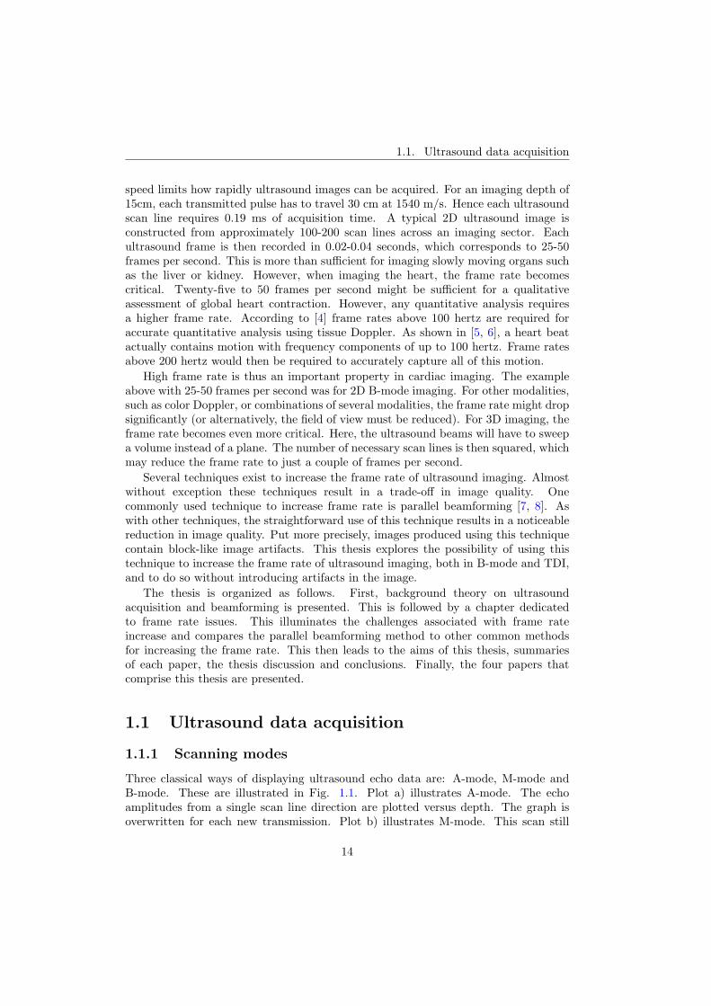
Three classical ways of displaying ultrasound echo data are: A-mode, M-mode andB-mode. These are illustrated in Fig. 1.1. Plot a) illustrates A-mode. The echoamplitudes from a single scan line direction are plotted versus depth. The graph isoverwritten for each new transmission. Plot b) illustrates M-mode. This scan still
14
Chapter 1. Introduction
Probe
OscillatingSphere inwater
Scan line
Depth
Dep
th
Dep
th
Ech
o A
mp
litu
de
Time
Lateral PositionProbe
a)
b)
c)
Figure 1.1: Imaging a oscillating sphere with three different scan modes. a) A-mode.Echo amplitude versus depth. b) M-mode. Gray tone coded echo amplitudes, depthversus time of transmission. c) B-mode. Gray tone coded echo amplitudes, depthversus lateral position.
has just one scan line direction, but the depth is now along the vertical axis and theecho amplitudes are plotted as gray tone coded vertical lines in the image. Whiteindicates strong echo and black no echo. The plot is continuously updated with a newvertical line for each new transmission. Hence, the horizontal axis shows the time ofeach transmission. Plot c) illustrates B-mode (Brightness mode). In this scan type,the echo intensities are also gray tone coded, but the directions of the scan lines arespread out over a sector to create a 2D still image of the object. The image shows depthalong the vertical axis and the lateral position of the scan line along the horizontalaxis. When doing live scanning, the plot will be continuously updated creating a livemovie of the object in the imaging sector.
1.1.2 Ultrasound transducer
The device that transmits and receives ultrasound is called a transducer and typicallycontains one or more piezoelectric elements. A piezoelectric material has the propertythat it contracts and expands when positive and negative voltages are applied. Byapplying a voltage alternating with the desired frequency, the piezoelectric elementstransform electric energy into acoustic energy and emit ultrasound at the desiredfrequency.
15

1.1. Ultrasound data acquisition
Piezo electric elements
Pitch Kerf
Figure 1.2: Illustration of a medical ultrasound transducer with piezoelectric elements.The number of elements is reduced for illustrational purposes. Typically such atransducer would have more than 100 elements.
Some transducers use only a single element to transmit ultrasound. However,most transducers contain an array of small elements since this provides the greatestflexibility in controlling the radiation pattern (See Fig. 1.2). Since each element issmall, they emit spherical sound waves. By controlling the amplitude and delay of thesignal for each element, the interference pattern created from all the spherical wavescan be controlled. Typically the radiation pattern is formed into a narrow, focusedand steered beam of sound.
1.1.3 Probe types
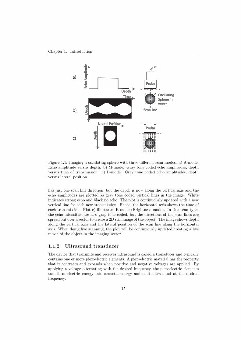
Different transducers are used for different applications. The most common transducertypes are shown in Fig. 1.3.
The probe in a) is called linear switched array. A linear array is typically quitewide and has large piezoelectric elements. The elements can be large compared to theultrasound wavelength, since this type of transducer typically does not steer the beam.Each scan line is created from beams pointing straight down from a varying origin onthe array. The array is called switched since it uses only a group of elements at onetime. The center of this group is slid across the transducer during a scan. A typicalapplication for such a probe is vascular imaging, i.e. imaging arteries and veins.
The probe in b) is called curved array. This type of array works in the same wayas a linear array. It is switched and uses a group of elements at a time. But since thesurface of the array is curved and each scan line is perpendicular to the surface, thistype of probe provides a wider field of view. This is useful in fetal imaging, or whenimaging internal organs such as the liver and kidney.
Probe c) in Fig. 1.3 is called a phased array. In such arrays all scan lines typicallyhave a fixed origin on the transducer surface, but are steered in a fan pattern to createthe image. These probes are typically smaller than linear and curved linear arrays.The reason for this is that they mostly are used for cardiac imaging where the footprinthas to fit between the ribs. Also, the elements of a phased array are smaller than forlinear arrays. This allows for larger steering angles without the unwanted interferencecalled grating lobes (Typical element sizes are around half the wavelength).
16
Chapter 1. Introduction
Dep
th
Lateral Position
Dep
th
Lateral Position
Dep
th
Lateral Position
a) b) c)
Figure 1.3: The most common probes used in medical ultrasound. a) Linear switchedarray. b) Linear curved array. c) Phased array.
1.1.4 Basic beamforming
An ultrasound B-mode image is constructed from the echo data of beams in severaldifferent directions. The term beam means that the ultrasound energy is focused inone specific direction and depth. This is enabled by the subdivision of the transducerinto elements. By adding delays to the electrical pulses sent to each element, theradiation pattern can be controlled. This type of beamforming is illustrated in Fig.1.4.
Plot a) shows the transmit beamforming. A signal generator sends a high frequencypulse to all channels of the system. Each channel has delay circuitry that adds anadjustable delay to the pulse. The delays are chosen so that the ultrasound wavesfrom each element arrive at the focal point simultaneously. This ensures high pressurethat gradually builds in the direction of the focal point, and reaches its maximumat this point (approximately). To the sides of the focal point, the ultrasound waveswill not be in phase. These locations will thus have lower amplitudes. For somedirections, the ultrasound waves will be in opposite phase and add destructively. Inthese directions the pressure will be zero (approximately).
Plot b) shows the receive beamforming. The principle here is exactly the same,only the process is reversed. A small point scatterer at the focus reflects incomingultrasound uniformly. These pressure waves propagate to the transducer and areconverted to electric signals by the piezoelectric elements. The delays are the same as
17

1.1. Ultrasound data acquisition
τ τ τ τ τ τ τ τ τ τ
Point scattererlocated in focus
Point scattererlocated outside focus
τ τ τ τ τ τ τ τ τ τ
a) Transmit b) Receive
Signal Generator
Delay
circuitry
c) Receive off axis target
τ τ τ τ τ τ τ τ τ τ
Figure 1.4: Transmit and receive beamforming. For all three illustrations, thetransducer is focused at the dotted cross. a) Transmit beamforming. b) Receivebeamforming with a point scatterer at the focus point. c) Receive beamforming witha point scatterer located outside the focus point.
when transmitting, and ensure that signals originating from the focal point are aligned.The aligned signals are then summed. Since they all are in phase, the resulting outputis amplified.
Plot c) shows what happens if the point scatterer is located outside the focal point.The transducer receive delays are adjusted to amplify signals originating from the focalpoint. Since this scatterer is located outside, the electrical pulses are not aligned afterthe delay circuitry. Hence they are summed out of phase, and the resulting outputis not amplified (in the illustrated case, the amplitude is actually decreased since thepoint scatterer is located close to a zero point).
1.1.5 Beam profiles
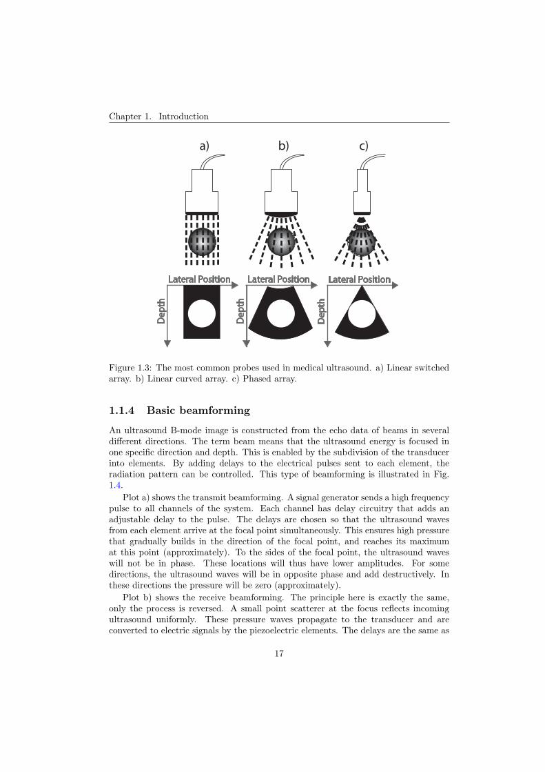
The transducer radiation pattern can be described using beam profiles. The top leftplot in Fig. 1.5 shows the pressure pulse measured along an equidistant arc at thefocal range (with time along the vertical axis and azimuth angle along the horizontalaxis). The corresponding beam profile shows the lateral energy distribution, and iscalculated as the mean square value of the pressure. In most cases the beam profiles
18
Chapter 1. Introduction
Transmit Receive pulse-echo
Figure 1.5: Beam profiles. Top figure row shows transducer responses along an arc atthe focal range. Bottom rows show the corresponding beam profiles. The left plotsshows the response and beam profile of the transmit aperture. The middle plots showthe receive response and beam profile. The right plots show the pulse-echo responseand beam profile.
are displayed in logarithmic scale. The central part of the beam profile is referred toas the main lobe. The parts of the beam profile outside the first zeros are referred toas the side lobes.
The top middle plot of Fig. 1.5 shows the receive response of the transducer atthe focal range. This corresponds to the signal received by this scan line from a pointsource emitting a spherical delta pulse located at focal range and at the angles specifiedby the horizontal axis. Since receiving is a passive process, the receive beam profilemaps the receive angle sensitivity instead of pressure.
The focal range pulse-echo response of the transducer is shown in the right plotof Fig. 1.5. This corresponds to the signal received by this scan line when imaging(transmitting and receiving) a point scatterer located at focal range and at the anglesspecified by the horizontal axis. Pulse-echo beam profiles thus show from which spatialextent scan lines get their echo data. Knowing the transmit and receive response, thepulse-echo response can be found from the temporal convolution between these two.The pulse-echo response is also referred to as the two-way response.
Fig. 1.5 only shows the beam profiles in the azimuth plane. Similar plots couldalso be made to describe the transducer sensitivity in the elevation plane.
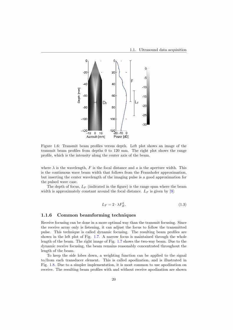
The beam profiles in Fig. 1.5 show beam profiles at a single range, the focal range.The left plot of Fig. 1.6 shows gray tone coded transmit beam profiles for all depthsfrom 0 to 120 mm. Such plots illustrate how the radiation field concentrates towardsthe focal depth. The right plot shows the intensity along the beam axis. Such plotsare referred to as range profiles, and show how the pressure (or sensitivity) builds uptowards the focus, and decays after.
The beam width DF , indicated in the left plot of Fig. 1.6 is calculated as [9]:
DF = F#λ, (1.1)
F# =F
a(1.2)
19
1.1. Ultrasound data acquisition
F
FLFD
Figure 1.6: Transmit beam profiles versus depth. Left plot shows an image of thetransmit beam profiles from depths 0 to 120 mm. The right plot shows the rangeprofile, which is the intensity along the center axis of the beam.
where λ is the wavelength, F is the focal distance and a is the aperture width. Thisis the continuous wave beam width that follows from the Fraunhofer approximation,but inserting the center wavelength of the imaging pulse is a good approximation forthe pulsed wave case.
The depth of focus, LF (indicated in the figure) is the range span where the beamwidth is approximately constant around the focal distance. LF is given by [9]:
LF = 2 · λF 2#, (1.3)
1.1.6 Common beamforming techniques
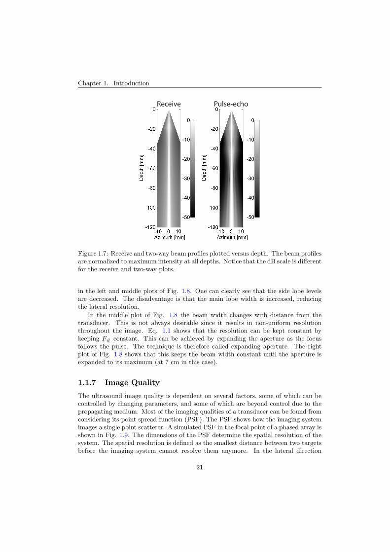
Receive focusing can be done in a more optimal way than the transmit focusing. Sincethe receive array only is listening, it can adjust the focus to follow the transmittedpulse. This technique is called dynamic focusing. The resulting beam profiles areshown in the left plot of Fig. 1.7. A narrow focus is maintained through the wholelength of the beam. The right image of Fig. 1.7 shows the two-way beam. Due to thedynamic receive focusing, the beam remains reasonably concentrated throughout thelength of the beam.
To keep the side lobes down, a weighting function can be applied to the signalto/from each transducer element. This is called apodization, and is illustrated inFig. 1.8. Due to a simpler implementation, it is most common to use apodization onreceive. The resulting beam profiles with and without receive apodization are shown
20
Chapter 1. Introduction
Receive Pulse-echo
Figure 1.7: Receive and two-way beam profiles plotted versus depth. The beam profilesare normalized to maximum intensity at all depths. Notice that the dB scale is differentfor the receive and two-way plots.
in the left and middle plots of Fig. 1.8. One can clearly see that the side lobe levelsare decreased. The disadvantage is that the main lobe width is increased, reducingthe lateral resolution.
In the middle plot of Fig. 1.8 the beam width changes with distance from thetransducer. This is not always desirable since it results in non-uniform resolutionthroughout the image. Eq. 1.1 shows that the resolution can be kept constant bykeeping F# constant. This can be achieved by expanding the aperture as the focusfollows the pulse. The technique is therefore called expanding aperture. The rightplot of Fig. 1.8 shows that this keeps the beam width constant until the aperture isexpanded to its maximum (at 7 cm in this case).
1.1.7 Image Quality
The ultrasound image quality is dependent on several factors, some of which can becontrolled by changing parameters, and some of which are beyond control due to thepropagating medium. Most of the imaging qualities of a transducer can be found fromconsidering its point spread function (PSF). The PSF shows how the imaging systemimages a single point scatterer. A simulated PSF in the focal point of a phased array isshown in Fig. 1.9. The dimensions of the PSF determine the spatial resolution of thesystem. The spatial resolution is defined as the smallest distance between two targetsbefore the imaging system cannot resolve them anymore. In the lateral direction
21

1.1. Ultrasound data acquisition
Element number
Gai
n
Element number
Without apodization With apodization
Element number
Gai
n
With apodization andexpanding aperture
Gai
n
Figure 1.8: Receive apodization and expanding aperture. The top image row showsthe aperture and its weighting function. The bottom image row shows the resultingreceive beams. The figure to the left shows the receive beam from using dynamicreceive focusing without apodization (identical to the two-way beam shown in Fig.1.7, but with a slightly different dynamic range). The middle plot shows the resultingreceive beam from applying receive apodization. The right plot shows the receivebeam from applying both receive apodization and expanding aperture.
(normal to the beam direction) the resolution is given by:
Δx =λF
atx + arx, (1.4)
where F is the focal range, λ is the center wavelength of the imaging pulse and atx
and arx are the size of the transmit and receive apertures. This equation is similarto Eq. 1.1, except that a is replaced with the two-way aperture, atx + arx, to get theactual imaging resolution. The radial resolution depends on the pulse length, and isgiven by:
Δr =c · Tpulse
2=
c
2 · Bpulse, (1.5)
where c is the speed of sound, Tpulse is the pulse length, and Bpulse is the frequencybandwidth of the pulse.
22

Chapter 1. Introduction
Figure 1.9: The point spread function of an imaging system. The left plot shows thePSF, and the right plot shows the location of the PSF in the field of view.
The image quality is also dependent on the contrast resolution of the system.The contrast resolution is a measure of how well the imaging system can differentiatebetween two regions with different scattering properties. An example could be anecho-free cyst embedded in tissue. Contrast resolution is determined by the side lobelevel of the PSF.
/2 element spacing element spacing
Figure 1.10: Grating lobes. The image to the left shows the image of a point scattererimaged with a λ/2 pitch array. The image to the right shows the same point scattererimaged with a λ pitch array. For the latter case, the large element spacing results ingrating lobes when the beams are steered. The scan lines to the far right of the imagethus pick up the point scatterer to the far left in their grating lobes. This causes thecloud emphasized with a surrounding oval in the image. Notice that the dB scale islarger than the normal 40dB. This was done deliberately to emphasize the effect ofgrating lobes.
Another type of side lobe that reduces the contrast resolution is grating lobes.Grating lobes are strong distant side lobes that appear if the pitch is too largecompared to the wavelength. A comparison between PSFs from arrays with pitchλ/2 and λ is shown in Fig. 1.10. The point scatterer located to the left is picked up
23
1.1. Ultrasound data acquisition
in the grating lobes of the scan lines to the right in the image.
1.1.8 Shift invariance
Shift invariance is an important property for an imaging system. In a shift invariantimaging system, the image of an object is independent of the object position relativeto the imaging aperture; i.e., the appearance of an object should not change when anobject moves. Hence, in a shift invariant imaging system, the PSF is identical at allpositions.
A conventional ultrasound system will not be globally shift invariant. Due tofocusing and steering, the PSF will slowly vary with position throughout the image.For the image quality of an ultrasound imaging system, it is most important withlocal shift invariance; i.e., the PSF should be constant over smaller areas of theimaging sector. This is important for object motion to be perceived correctly inimage sequences.
1.1.9 Body wall distortion effects
The beamforming delays are adjusted to ensure that the ultrasound waves from allelements arrive at the focal point at the same time. It is then assumed that thepropagation velocity is constant. This is not the case when imaging through the bodywall. The ultrasound waves propagate through fat, muscle, blood and connectivetissue, which all have different speeds of sound. This causes distortions to theultrasound wave front, which are referred to as aberrations. These distortions typicallyreduce the focusing effect and result in a lower main lobe level and reduced contrastresolution.
Another beamforming assumption is that the ultrasound pulse is reflected onlyone time. In practice, the pulse is reflected several times between tissue layers beforereturning to the transducer. The increased propagation time of echoes reflectedmultiple times will make them arrive simultaneously with direct echoes from moredistant locations, which combined reduce the contrast resolution. Multiple reflectionsare also called reverberations and are especially visible in the near field due to thelayered structure of the tissue close to the skin. Here they appear as a haze over theimaged structures.
1.1.10 Biomechanical effects of ultrasound
If applied with enough power, ultrasound waves can be harmful. An example is thetherapeutic ultrasound that is used to shatter kidney stones. Another example is high-intensity focused ultrasound, HIFU. HIFU can be used to perform surgery inside thebody, specifically to produce highly localized lesions.
There are two biomechanical effects of transmitting ultrasound into tissue. Thefirst effect is a temperature increase. The energy from ultrasound is absorbed by thetissue as heat. The temperature increase from ultrasound exposure is described by
24
Chapter 1. Introduction
the thermal index, TI [10]:
TI =W0
Wdeg, (1.6)
where W0 is the time-averaged acoustic power of the source (or another powerparameter), and Wdeg is the power necessary to raise the target temperature by 1◦Cbased on specific thermal and tissue models.
The second biomechanical effect is cavitation. Cavitation is the creation of gasbubbles in the tissue. This can occur if the peak negative pressure of the ultrasoundpulse is too high. The mechanical index, MI, is an estimate of the likelihood ofcavitation, and is given by [10]:
MI =Pr.3√
fc, (1.7)
where Pr.3 is a measure of the peak negative pressure and fc the center frequency ofthe imaging pulse (See [10] for details).
From an image quality point of view, it would be beneficial to use a high transmitpower. This would increase the penetration and increase the signal-to-noise ratio ofthe received signal. However, to avoid harmful biomechanical effects, the maximumallowed MI and TI for ultrasound equipment used for medical imaging are under strictregulations.
1.1.11 Sampling
To be able to perfectly reconstruct a sampled signal, the Nyquist sampling theoremstates that the sampling frequency must be at least twice the highest frequencycomponent in the signal. This puts constraints on the sampling frequency whendigitalizing the received ultrasound echoes, but it also puts constraints on the spacingbetween the ultrasound beams. From the Fraunhofer approximation, it follows thatthe Fourier transform of a continuous wave ultrasound field in focus is given by theaperture shape and size, and the wavelength. This gives us the lateral bandwidthof each frequency component in pulsed wave transmission and the following Nyquistbeam spacing requirements for transmit and two-way beams (in radians):
δθtnq =
λ
atx, (1.8)
δθtrnq =
λ
atx + arx, (1.9)
where λ is the wavelength and atx and arx are the transmit and receive aperturesizes. To achieve lossless insonification and sampling of an object, both theseconstraints must be met. If not, azimuthal information will be lost, and the resultingimage will contain aliasing artifacts. The typical indication of under sampling andaliasing is that the imaging system becomes locally shift variant, i.e. the PSF varieswith small changes in position.
25
1.2. Frame Rate
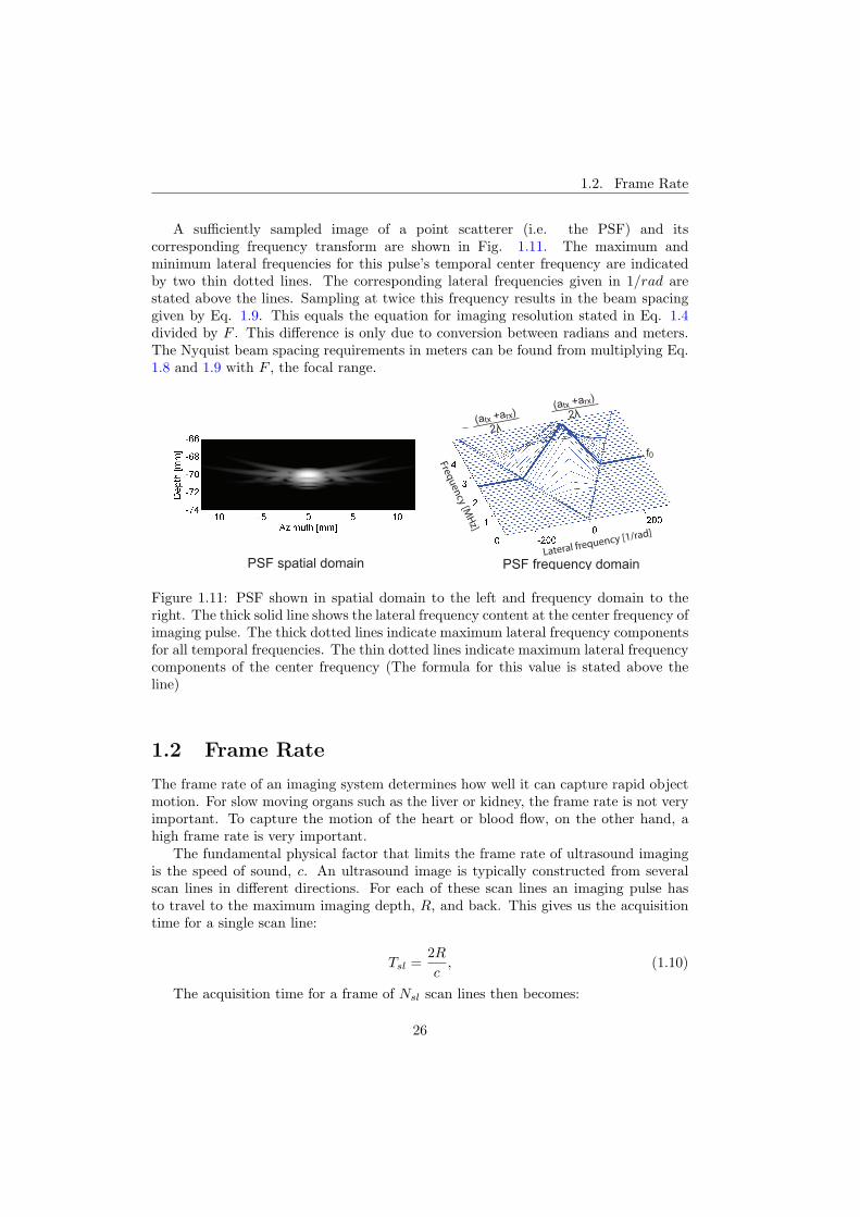
A sufficiently sampled image of a point scatterer (i.e. the PSF) and itscorresponding frequency transform are shown in Fig. 1.11. The maximum andminimum lateral frequencies for this pulse’s temporal center frequency are indicatedby two thin dotted lines. The corresponding lateral frequencies given in 1/rad arestated above the lines. Sampling at twice this frequency results in the beam spacinggiven by Eq. 1.9. This equals the equation for imaging resolution stated in Eq. 1.4divided by F . This difference is only due to conversion between radians and meters.The Nyquist beam spacing requirements in meters can be found from multiplying Eq.1.8 and 1.9 with F , the focal range.
Lateral frequency [1/rad]
Frequency [MH
z]
PSF spatial domain PSF frequency domain
(atx +arx)(atx +arx)
f0
Figure 1.11: PSF shown in spatial domain to the left and frequency domain to theright. The thick solid line shows the lateral frequency content at the center frequency ofimaging pulse. The thick dotted lines indicate maximum lateral frequency componentsfor all temporal frequencies. The thin dotted lines indicate maximum lateral frequencycomponents of the center frequency (The formula for this value is stated above theline)
1.2 Frame Rate
The frame rate of an imaging system determines how well it can capture rapid objectmotion. For slow moving organs such as the liver or kidney, the frame rate is not veryimportant. To capture the motion of the heart or blood flow, on the other hand, ahigh frame rate is very important.
The fundamental physical factor that limits the frame rate of ultrasound imagingis the speed of sound, c. An ultrasound image is typically constructed from severalscan lines in different directions. For each of these scan lines an imaging pulse hasto travel to the maximum imaging depth, R, and back. This gives us the acquisitiontime for a single scan line:
Tsl =2R
c, (1.10)
The acquisition time for a frame of Nsl scan lines then becomes:
26
Chapter 1. Introduction
Tfr = Tsl · Nsl =2R
c· Nsl. (1.11)
Assuming an equal transmit and receive aperture, atx = arx, transmit samplingcriterion will be satisfied when the two-way criterion is satisfied (Eq. 1.9). Thenumber of scan lines, Nsln, necessary to sufficiently sample a sector φ (in radians)then becomes:
Nsln =φ
δθtrnq
=φ · (atx + arx)
λ. (1.12)
Before the ultrasound echoes are displayed as gray tone coded B-mode, the echoeswill be detected (squared value of the envelope) and log-compressed. This processeffectively doubles the lateral bandwidth of the echo data. To avoid aliasing from thisprocess, one will have to acquire twice the number of scan lines, Nsln, stated in Eq.1.12. Inverting Eq. 1.11 and inserting 2 · Nsln for Nsl then gives us the maximumframe rate of a sufficiently sampled image scan:
ffr =1
Tfr=
12 · Nsln · Tsl
=cλ
4Rφ · (atx + arx). (1.13)
If inserting typical cardiac parameters (c = 1540m/s, f0 = 2.5MHz, λ = c/f0 =0.616mm, R = 15cm, φ = 75deg, atx = 2cm, arx = 2cm), the resulting frame rate fromthis formula will be 30 frames per second.
The following sections review selected methods for increasing the frame rate.
1.2.1 IQ interpolation
In the term IQ data, the ”I” stands for in phase, and ”Q” for quadrature. TheIQ ultrasound data is simply the complex base band version of the echo data,i.e., the received echo data demodulated and bandpass filtered (without any loss ofinformation). This is a commonly used and convenient format for further processingof the ultrasound data.
The concept of IQ interpolation is to double (or more) the amount of scan linesbefore the detection stage. By doing this, the echo data will also be sufficiently sampledafter the lateral bandwidth doubling in the detection stage. This way, the Nsln scanlines of Eq. 1.12 will be sufficient, resulting in a doubling of the frame rate in Eq.1.13.
However, since the interpolation is done coherently, IQ interpolation will besensitive to motion. If the object has moved sufficiently in the time span between twoneighboring scan lines, these two scan lines can in the worst case be out of phase. Thiswould result in the interpolated scan line amplitude being zero. For less motion, theamplitude of the interpolated scan lines will be reduced. Due to this, IQ interpolationand object motion can lead to artifacts in the B-mode images.
27
1.2. Frame Rate
Transmit 1
SLA 4MLA
Transmit 2
Transmit 3
Scan lines
Beam angleBeam angle
Time
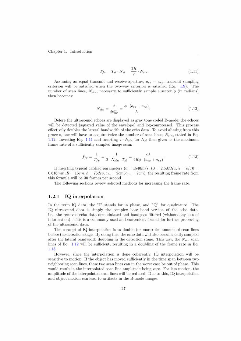
Figure 1.12: Comparison of single line acquisition, SLA, and multiple line acquisition,MLA. SLA is shown to the left, MLA to the right. Down arrows indicate transmitdirection and up arrows receive directions. For SLA, transmit and receive directionsare identical. The resulting scan line directions are indicated with lines at the bottomof the illustration.
1.2.2 Multiple Line Acquisition, MLA
The concept of MLA is to acquire more than one scan line for each transmit event[7, 8]. This is also called parallel beamforming (multiple parallel receive beams foreach transmit beam). This allows for fewer transmit events with the same amount ofscan lines. The concept is illustrated for four parallel beams, 4MLA, in Fig. 1.12. Thepotential frame rate increase compared to conventional single line acquisition, SLA, isequal to the number of parallel beams.
Using this technique, a frame could theoretically be acquired from one transmitpulse illuminating the whole object and beamform in all receive directions at once.However, there are several reasons why this is not an especially good idea:
1. Reduced image resolution. To illuminate the whole object with a single pulse,the transmit beam would have to be wide. This corresponds to using a verysmall transmit aperture. From Eq. 1.4, one can see that the resolution then isreduced to the resolving power of the receive beam alone (λF/arx).
2. Higher side lobes. The resulting two-way side lobe level will be identical to theside lobe level of the receive beam alone (-14dB). The side lobes of a normaltwo-way beam are located 28 dB below the main lobe level (See Fig. 1.5). Thisresults in a heavily reduced contrast resolution. Applying receive apodizationcould compensate for this, but that would reduce the resolution further.
3. Reduced penetration. Transmitting an unfocused pulse instead of a focusedpulse reduces the allowed transmit power according to the maximum limit for themechanical index, MI. The MI limit is calculated from maximum axial pressure,and while a focused transmit pulse has its maximum deep in the tissue, anunfocused transmit pulse has its maximum at the transducer surface. Hence,the signal-to-noise ratio will be much poorer in the lower parts of the ultrasoundimage using an unfocused transmit pulse than a focused transmit pulse.
28
Chapter 1. Introduction
4. Increased hardware requirements. Beamforming all receive beams real time foreach transmit event puts high requirements on the hardware.
From this it can be concluded that it is beneficial to generate transmit beams thatare as focused as possible for maximum image quality.
When applying MLA to reduce the number of transmit beams, the transmitaperture, atx, must be adjusted to satisfy the Nyquist transmit beam spacingrequirements stated in Eq. 1.8. The first paper in this thesis presents an equation forthe necessary number of parallel beams given Nyquist oversampling factors pt and ptr
for the transmit and two-way beam spacing. For transmit and receive apertures atx
and arx this relation is given by:
NmlaN =pt
ptr· (1 +
arx
atx). (1.14)
This equation shows that for two parallel beams and marginal sampling (pt =ptr = 1), no reduction in transmit aperture is required, resulting in twice the framerate without loss in image resolution, contrast resolution or penetration. However,using four parallel beams and marginal sampling (i.e. a fourfold increase in framerate), the transmit aperture will have to be reduced to 1/3 of the receive aperture.The image quality will then start to suffer from the three first issues listed above.
It can be mentioned here that Eq. 1.14 assumes that IQ interpolation is used toavoid aliasing from the detection stage. If not, NmlaN should be multiplied by a factorof two. Using four parallel beams without IQ interpolation could then give a framerate four times higher than that of the SLA case in Eq. 1.13 without having to reducethe transmit aperture. By doing this, one also avoids the potential problem of motionartifacts using IQ interpolation.
The main problem resulting from applying parallel beamforming is, however, theblock-like artifacts in the B-mode image. The mechanisms of these artifacts will bediscussed in chapter 1.3.
1.2.3 Multiple Line Transmission, MLT
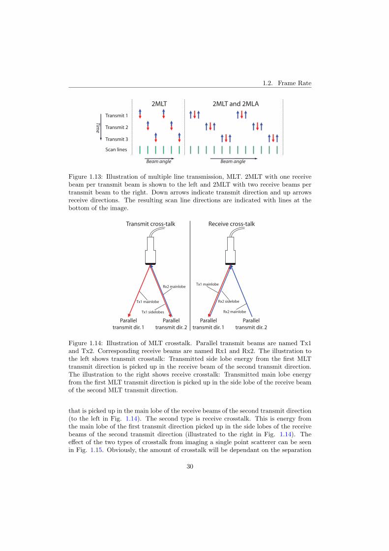
The concept behind MLT is to transmit in several directions simultaneously. As isshown in Fig. 1.13, this technique can be combined with MLA to also acquire multiplescan lines for each transmit beam. For the case shown to the right in the figure, thenumber of transmit events is reduced by a factor of four compared to conventionalSLA.
An advantage of MLT is an even higher achievable frame rate before the transmitaperture has to be reduced. According to Eq. 1.14, the frame rate can be increasedby a factor of two times the number of parallel transmit beams without reductions tothe transmit aperture when combined with 2MLA. Alternatively, a factor four timesthe number of parallel transmit beams if IQ interpolation is not used.
A disadvantage of MLT is the crosstalk between the parallel transmit beams. Thecrosstalk can be split into two types, as illustrated in Fig. 1.14. The first type istransmit crosstalk. This is energy from the side lobe of the first transmit direction
29
1.2. Frame Rate
Transmit 1
2MLT 2MLT and 2MLA
Transmit 2
Transmit 3
Scan lines
Beam angleBeam angle
Time
Figure 1.13: Illustration of multiple line transmission, MLT. 2MLT with one receivebeam per transmit beam is shown to the left and 2MLT with two receive beams pertransmit beam to the right. Down arrows indicate transmit direction and up arrowsreceive directions. The resulting scan line directions are indicated with lines at thebottom of the image.
Transmit cross-talk
Paralleltransmit dir. 1
Paralleltransmit dir. 2
Receive cross-talk
Paralleltransmit dir. 1
Paralleltransmit dir. 2
Tx1 sidelobes
Tx1 mainlobe
Rx2 mainlobe
Rx2 mainlobe
Rx2 sidelobe
Tx1 mainlobe
Figure 1.14: Illustration of MLT crosstalk. Parallel transmit beams are named Tx1and Tx2. Corresponding receive beams are named Rx1 and Rx2. The illustration tothe left shows transmit crosstalk: Transmitted side lobe energy from the first MLTtransmit direction is picked up in the receive beam of the second transmit direction.The illustration to the right shows receive crosstalk: Transmitted main lobe energyfrom the first MLT transmit direction is picked up in the side lobe of the receive beamof the second MLT transmit direction.
that is picked up in the main lobe of the receive beams of the second transmit direction(to the left in Fig. 1.14). The second type is receive crosstalk. This is energy fromthe main lobe of the first transmit direction picked up in the side lobes of the receivebeams of the second transmit direction (illustrated to the right in Fig. 1.14). Theeffect of the two types of crosstalk from imaging a single point scatterer can be seenin Fig. 1.15. Obviously, the amount of crosstalk will be dependant on the separation
30
Chapter 1. Introduction
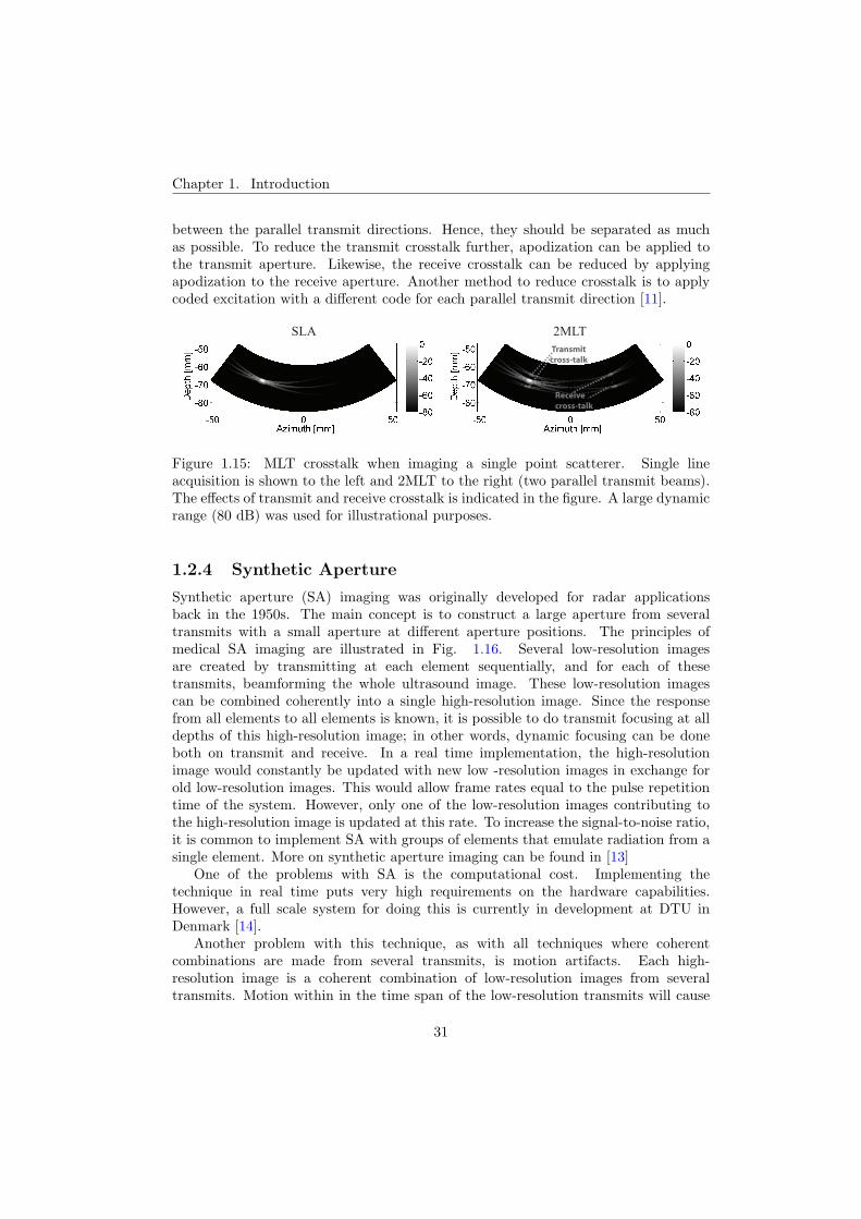
between the parallel transmit directions. Hence, they should be separated as muchas possible. To reduce the transmit crosstalk further, apodization can be applied tothe transmit aperture. Likewise, the receive crosstalk can be reduced by applyingapodization to the receive aperture. Another method to reduce crosstalk is to applycoded excitation with a different code for each parallel transmit direction [11].
SLA 2MLTTransmitcross-talk
Receivecross-talk
Figure 1.15: MLT crosstalk when imaging a single point scatterer. Single lineacquisition is shown to the left and 2MLT to the right (two parallel transmit beams).The effects of transmit and receive crosstalk is indicated in the figure. A large dynamicrange (80 dB) was used for illustrational purposes.
1.2.4 Synthetic Aperture
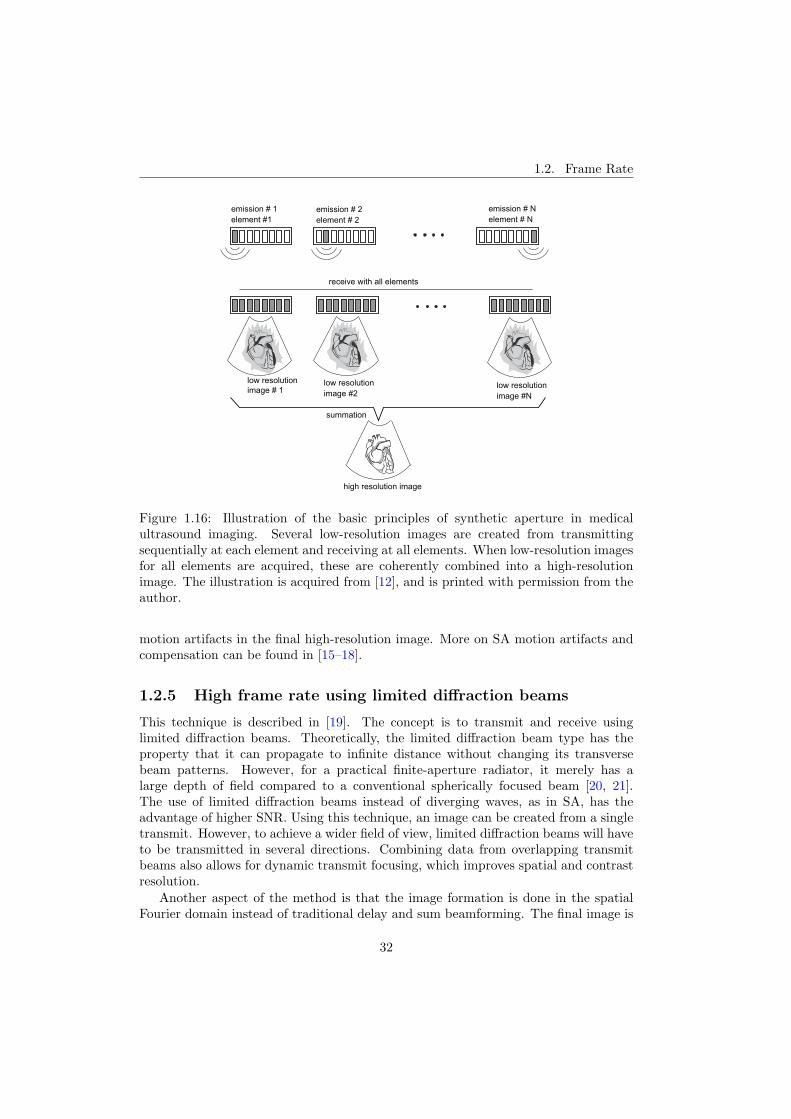
Synthetic aperture (SA) imaging was originally developed for radar applicationsback in the 1950s. The main concept is to construct a large aperture from severaltransmits with a small aperture at different aperture positions. The principles ofmedical SA imaging are illustrated in Fig. 1.16. Several low-resolution imagesare created by transmitting at each element sequentially, and for each of thesetransmits, beamforming the whole ultrasound image. These low-resolution imagescan be combined coherently into a single high-resolution image. Since the responsefrom all elements to all elements is known, it is possible to do transmit focusing at alldepths of this high-resolution image; in other words, dynamic focusing can be doneboth on transmit and receive. In a real time implementation, the high-resolutionimage would constantly be updated with new low -resolution images in exchange forold low-resolution images. This would allow frame rates equal to the pulse repetitiontime of the system. However, only one of the low-resolution images contributing tothe high-resolution image is updated at this rate. To increase the signal-to-noise ratio,it is common to implement SA with groups of elements that emulate radiation from asingle element. More on synthetic aperture imaging can be found in [13]
One of the problems with SA is the computational cost. Implementing thetechnique in real time puts very high requirements on the hardware capabilities.However, a full scale system for doing this is currently in development at DTU inDenmark [14].
Another problem with this technique, as with all techniques where coherentcombinations are made from several transmits, is motion artifacts. Each high-resolution image is a coherent combination of low-resolution images from severaltransmits. Motion within in the time span of the low-resolution transmits will cause
31
1.2. Frame Rate
element #1 element # 2emission # 2emission # 1 emission # N
element # N
receive with all elements
low resolution image #2
low resolutionimage #N
low resolution image # 1
summation
high resolution image
Figure 1.16: Illustration of the basic principles of synthetic aperture in medicalultrasound imaging. Several low-resolution images are created from transmittingsequentially at each element and receiving at all elements. When low-resolution imagesfor all elements are acquired, these are coherently combined into a high-resolutionimage. The illustration is acquired from [12], and is printed with permission from theauthor.
motion artifacts in the final high-resolution image. More on SA motion artifacts andcompensation can be found in [15–18].
1.2.5 High frame rate using limited diffraction beams
This technique is described in [19]. The concept is to transmit and receive usinglimited diffraction beams. Theoretically, the limited diffraction beam type has theproperty that it can propagate to infinite distance without changing its transversebeam patterns. However, for a practical finite-aperture radiator, it merely has alarge depth of field compared to a conventional spherically focused beam [20, 21].The use of limited diffraction beams instead of diverging waves, as in SA, has theadvantage of higher SNR. Using this technique, an image can be created from a singletransmit. However, to achieve a wider field of view, limited diffraction beams will haveto be transmitted in several directions. Combining data from overlapping transmitbeams also allows for dynamic transmit focusing, which improves spatial and contrastresolution.
Another aspect of the method is that the image formation is done in the spatialFourier domain instead of traditional delay and sum beamforming. The final image is
32
Chapter 1. Introduction
created from an inverse Fourier transform.At the cost of reduced lateral resolution, it is also possible to transmit plane waves
instead of limited diffraction beams [22].
1.3 MLA artifacts
Cardiac 4MLACardiac SLA
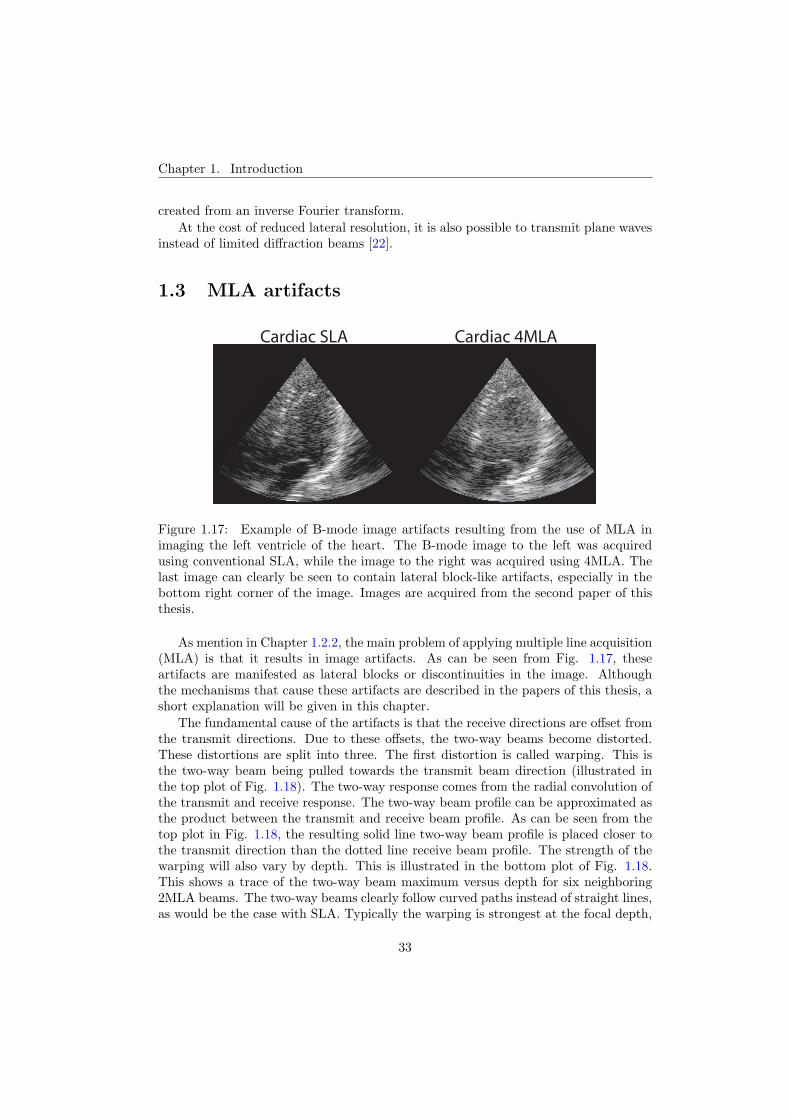
Figure 1.17: Example of B-mode image artifacts resulting from the use of MLA inimaging the left ventricle of the heart. The B-mode image to the left was acquiredusing conventional SLA, while the image to the right was acquired using 4MLA. Thelast image can clearly be seen to contain lateral block-like artifacts, especially in thebottom right corner of the image. Images are acquired from the second paper of thisthesis.
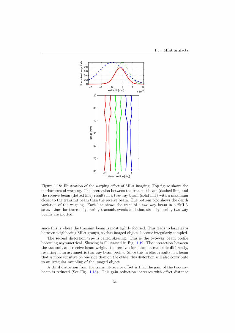
As mention in Chapter 1.2.2, the main problem of applying multiple line acquisition(MLA) is that it results in image artifacts. As can be seen from Fig. 1.17, theseartifacts are manifested as lateral blocks or discontinuities in the image. Althoughthe mechanisms that cause these artifacts are described in the papers of this thesis, ashort explanation will be given in this chapter.
The fundamental cause of the artifacts is that the receive directions are offset fromthe transmit directions. Due to these offsets, the two-way beams become distorted.These distortions are split into three. The first distortion is called warping. This isthe two-way beam being pulled towards the transmit beam direction (illustrated inthe top plot of Fig. 1.18). The two-way response comes from the radial convolution ofthe transmit and receive response. The two-way beam profile can be approximated asthe product between the transmit and receive beam profile. As can be seen from thetop plot in Fig. 1.18, the resulting solid line two-way beam profile is placed closer tothe transmit direction than the dotted line receive beam profile. The strength of thewarping will also vary by depth. This is illustrated in the bottom plot of Fig. 1.18.This shows a trace of the two-way beam maximum versus depth for six neighboring2MLA beams. The two-way beams clearly follow curved paths instead of straight lines,as would be the case with SLA. Typically the warping is strongest at the focal depth,
33
1.3. MLA artifacts
−2 −1 0 1 2 3
x 10−3
0
0.2
0.4
0.6
0.8
Azimuth [mm]
Nor
mal
ized
am
plitu
de
−2 0 2
20
30
40
50
60
70
80
Lateral position [deg]
Ran
ge [m
m]
Figure 1.18: Illustration of the warping effect of MLA imaging. Top figure shows themechanisms of warping. The interaction between the transmit beam (dashed line) andthe receive beam (dotted line) results in a two-way beam (solid line) with a maximumcloser to the transmit beam than the receive beam. The bottom plot shows the depthvariation of the warping. Each line shows the trace of a two-way beam in a 2MLAscan. Lines for three neighboring transmit events and thus six neighboring two-waybeams are plotted.
since this is where the transmit beam is most tightly focused. This leads to large gapsbetween neighboring MLA groups, so that imaged objects become irregularly sampled.
The second distortion type is called skewing. This is the two-way beam profilebecoming asymmetrical. Skewing is illustrated in Fig. 1.19. The interaction betweenthe transmit and receive beam weights the receive side lobes on each side differently,resulting in an asymmetric two-way beam profile. Since this in effect results in a beamthat is more sensitive on one side than on the other, this distortion will also contributeto an irregular sampling of the imaged object.
A third distortion from the transmit-receive offset is that the gain of the two-waybeam is reduced (See Fig. 1.18). This gain reduction increases with offset distance
34

Chapter 1. Introduction
−4 −3 −2 −1 0 1 2 3 4
−40
−35
−30
−25
−20
−15
−10
−5
0
Angle [deg]
RM
S p
ower
[dB
]
Transmit and Receive Beam Profiles
Two wayTransmitReceive
Figure 1.19: Illustration of the skewing effect using MLA. The interaction betweenthe transmit beam (dashed line) and the offset receive beam (dotted line) results inan asymmetrical two-way beam profile (solid line).
and results in a lateral gain modulation in the B-mode image (when imaging withmore than two parallel beams).
Techniques to compensate for these parallel beamforming artifacts have previouslybeen proposed by others [23–29]. A common factor among all these proposals is thatthey are contained in commercial patents and not in academic papers. As patents areonly designed to describe techniques, the information provided offers little insight intothe actual performance. Performance evaluations of several compensation techniqueswill be presented in the papers of this thesis.
1.4 Tissue Doppler Imaging
Tissue Doppler imaging, TDI, is an imaging modality that estimates tissue velocities.It was first introduced by McDicken et al. in 1992 [30]. Since then, TDI has become acommon imaging modality among cardiologists since it enables quantitative evaluationof cardiac tissue function.
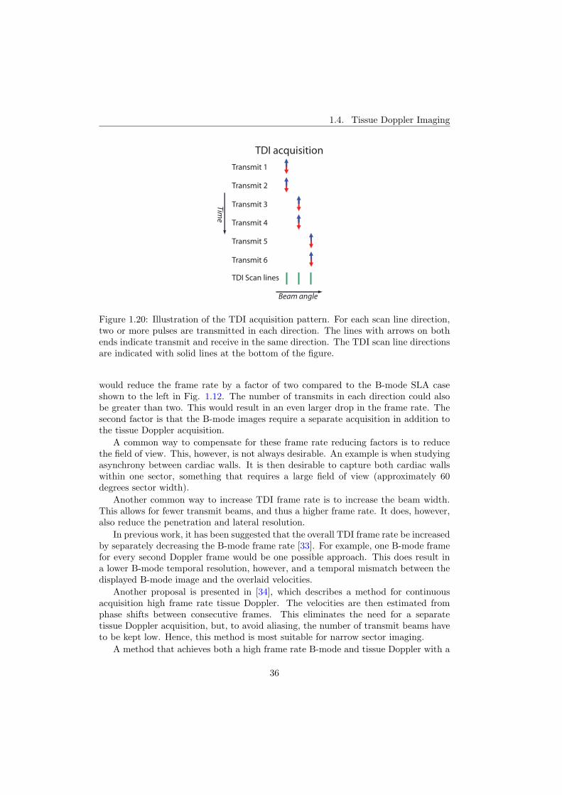
The principles of TDI are similar to those of Color Flow imaging [31]. Severalpulses are transmitted in each direction, and the phase shifts between the receive dataare calculated to estimate motion (See Fig. 1.20). The autocorrelation method [32] ismost commonly used to estimate the phase shift.
It is common to also acquire B-mode images along with the tissue Doppler images.These images are combined into a single color-coded image displaying both tissueintensity and tissue velocities. Due to rapid tissue deformation, frame rates above 100Hz are desired in cardiac TDI [4]. There are two factors limiting the TDI frame rate.The first is that tissue Doppler data require several transmissions in each direction.For the case illustrated in Fig. 1.20, two transmits are used in each direction. This
35
1.4. Tissue Doppler Imaging
Transmit 1
TDI acquisition
Transmit 2
Transmit 3
TDI Scan lines
Beam angle
Time
Transmit 4
Transmit 5
Transmit 6
Figure 1.20: Illustration of the TDI acquisition pattern. For each scan line direction,two or more pulses are transmitted in each direction. The lines with arrows on bothends indicate transmit and receive in the same direction. The TDI scan line directionsare indicated with solid lines at the bottom of the figure.
would reduce the frame rate by a factor of two compared to the B-mode SLA caseshown to the left in Fig. 1.12. The number of transmits in each direction could alsobe greater than two. This would result in an even larger drop in the frame rate. Thesecond factor is that the B-mode images require a separate acquisition in addition tothe tissue Doppler acquisition.
A common way to compensate for these frame rate reducing factors is to reducethe field of view. This, however, is not always desirable. An example is when studyingasynchrony between cardiac walls. It is then desirable to capture both cardiac wallswithin one sector, something that requires a large field of view (approximately 60degrees sector width).
Another common way to increase TDI frame rate is to increase the beam width.This allows for fewer transmit beams, and thus a higher frame rate. It does, however,also reduce the penetration and lateral resolution.
In previous work, it has been suggested that the overall TDI frame rate be increasedby separately decreasing the B-mode frame rate [33]. For example, one B-mode framefor every second Doppler frame would be one possible approach. This does result ina lower B-mode temporal resolution, however, and a temporal mismatch between thedisplayed B-mode image and the overlaid velocities.
Another proposal is presented in [34], which describes a method for continuousacquisition high frame rate tissue Doppler. The velocities are then estimated fromphase shifts between consecutive frames. This eliminates the need for a separatetissue Doppler acquisition, but, to avoid aliasing, the number of transmit beams haveto be kept low. Hence, this method is most suitable for narrow sector imaging.
A method that achieves both a high frame rate B-mode and tissue Doppler with a
36
Chapter 1. Introduction
wide imaging sector will be presented in the last paper of this thesis.
1.5 Motivation and aims of study
The main motivation for this thesis is the need for higher frame rate in cardiacultrasound imaging. Parallel beamforming is a promising technique for achievingthis, but as pointed out in the introduction, this method suffers from B-mode imageartifacts. Previous work performed on removing these artifacts is mainly containedwithin commercial patents, hence little information exists on the mechanisms of theseartifacts or on metrics to evaluate and quantify them. As patents are aimed atdescribing rather than evaluating, they also provide little information about the actualperformance of the methods in practical, realistic scenarios. Academic work on thissubject is thus in short supply.
Combined modes, such as TDI, where combined B-mode and tissue Doppler dataare acquired using separate acquisitions, reduce the frame rate. Since high frame ratesare necessary for TDI quantitative analysis, this problem is often solved by reducingthe field of view or reducing the image quality in the B-mode or tissue Doppler.
The aims of this thesis are to:
Aim 1: Indentify the mechanisms of parallel beamforming artifact and develop metricsto evaluate these mechanisms.
Aim 2: Investigate possibilities for artifact compensation and evaluate theirperformance using the developed metrics.
Aim 3: Investigate the performance of the compensation techniques in realistic,aberrating scenarios.
Aim 4: Address the possibilities of increasing the frame rate of combined tissueDoppler and B-mode imaging.
1.6 Summary of presented work
The following subsections contain summaries of the papers in this thesis. They arelisted in the order the research was performed, which is not necessarily the order ofpublication. The third paper is in a review process and has recently been resubmittedafter a revision. The fourth paper is unpublished, but has recently been submitted forpublication in a peer-reviewed journal.
37
1.6. Summary of presented work
Paper no. 1:Parallel beamforming using synthetic transmit beams
This paper addressed the fundamental source of parallel beamforming artifacts, namelythe misalignment of the transmit and receive beams. This misalignment results indistortions to the ultrasound imaging beam that varies both with depth and frombeam to beam. Due to this, parallel beamforming imaging systems are not spatiallyshift invariant; i.e. the image of an object varies with the object location. Toremove distortions to the ultrasound beams and restore shift invariance, this worksuggested creating synthetic transmit beams in the direction of each receive beam.The fundamental implementation of this technique is to create the synthetic transmitbeams from interpolation on the unfocused channel data prior to beamforming. Thiswork showed that an identical, but more practical feasible implementation can beperformed after beamforming by receiving two times in each direction in neighboringtransmit events. The proposed STB method was compared to other compensationmethods through simulations and in vitro recordings. To evaluate the shift varianceof the various methods, the paper introduced a plot that was later called the lateralshift variance plot (LSV plot). The paper also presented a formula for calculatingthe number of necessary parallel beams from the size of the transmit and receiveapertures. The main result was that STB results in a more shift invariant imagingsystem with suppressed MLA artifacts. The paper also concluded that one of theother compensation methods, dynamic steering, appears to be a promising techniquefor removing MLA artifacts.
The work was a joint effort with PhD student Torbjørn Hergum. Torbjørn Hergumconducted the theoretical work, illustrations and most of the writing. The author’smain responsibilities were simulations, figures and quantitative results.
This paper was published in IEEE Transactions on Ultrasonics, Ferroelectrics, andFrequency Control, vol. 54, February 2007.
Paper no. 2:The impact of aberration on high frame rate cardiac B-mode imaging
This paper investigated the effect of aberration on parallel beamforming and dynamicsteering as an MLA artifact compensation method. The B-mode artifacts of parallelbeamforming are rooted in the misalignment of the transmit and receive beams. Thiscauses the two-way beams to follow curved trajectories; i.e., the maximums of thetwo-way beam profiles are pulled towards the transmit beam directions. This is calledwarping. From models or simulations, the warping can be estimated, and the receivebeams can be additionally offset to counteract the effect. This is the concept behindthe dynamic steering method. The previous paper concluded that this was a promisingtechnique for reducing MLA artifacts. This paper showed that although successful inideal environments such as simulations and in-vitro recordings, the dynamic steeringcompensation fails in the presence of aberration. The mechanisms were investigatedand explained through lateral shift variance plots, beam profile simulations, B-mode
38
Chapter 1. Introduction
simulations, in-vitro recordings and in vivo recordings. To measure the amount ofartifacts in the B-mode image, this work introduced a new metric based on beam-to-beam correlation.
The work was a joint effort with PhD Svein Arne Aase. Svein Arne Aase’s mainresponsibility was scanner modifications and recording analysis. The author’s mainresponsibility was simulations.
This paper was published in IEEE Transactions on Ultrasonics, Ferroelectrics, andFrequency Control, vol. 54, January 2007.
Paper no. 3:Synthetic transmit beam technique in an aberrating environment
Paper 2 showed that dynamic steering fails as an MLA artifact compensation methodin aberrating environments. In this paper, the performance of the STB methodwas investigated in the presence of aberration. Given ideal STB interpolation, theonly theoretical requirement for the STB method to work is that the transmit beamspacing satisfies the lateral Nyquist sampling theorem. Simple aberrations close tothe transducer surface can be modeled as modifications to the transducer aperture.Such modifications do not increase the lateral bandwidth, and thus do not affect thesampling requirements. This work investigated STB performance with aberrationswhen using linear STB interpolation. The work was also a continuation of the firstpaper on STB. The number of parallel beams was increased from two to four, and newperformance metrics such as speckle tracking error, higher order STB interpolation,beam profile shape conservation and beam-to-beam correlation are applied. Theresults showed that while aberration increases the image artifacts of conventionalparallel beamforming, the usage of STB resulted in low levels of image artifacts bothwith and without aberration. This was also reflected in the speckle tracking errors,which increased with aberration for conventional parallel beamforming. Using STBthe tracking error was almost unchanged. The LSV plots showed that using STB alsoresulted in close to shift invariance with aberration. Higher order STB interpolationfurther improved shift invariance, but might not be feasible due to potential motionartifacts. The beam profile shape was better preserved using STB. This was alsoreflected in the improved beam-to-beam correlation consistency.
This paper is under review with IEEE Transactions on Ultrasonics, Ferroelectrics,and Frequency Control.
Paper no. 4:Single pulse tissue Doppler using synthetic transmit beams
While the previous papers focused on the amplitude of the echoes using parallelbeamforming, this work focused on the phase of the echoes. More specifically, this workexplored the possibility of estimating tissue velocities using the STB acquisition. Thiswas enabled by double reception in each scan line direction. Since the proposed method
39
1.7. Discussion
estimated the velocities from phase shifts between spatially neighboring transmitevents, the method was named Single Pulse Tissue Doppler, SPTD. This methodalso included a novel transmit beam interleaving pattern, allowing the Nyquist limitto be adapted to cardiac velocities without loss in frame rate. The work addressed twoproblems of the SPTD method, namely the estimation bias and the higher estimationvariance compared to regular TDI. The most noticeable problem with SPTD is theestimation bias which varies both from beam to beam and with depth. Throughsimulations, it was shown that the SPTD bias originated from lateral phase variationsacross the transmit beam. Model-based averaging was proposed as compensation.Warping and skewing resulted in decorrelation between scan lines in the same direction.This increased the estimation variance compared to regular TDI. However, if biascompensation and moderate radial averaging are applied, the accuracy of the SPTDvelocity estimates are close to those of regular TDI. The use of the SPTD methodresulted in combined B-mode and tissue Doppler images of the whole left ventricle ata frame rate of 110 frames per second.
This paper has been submitted for publication in IEEE Transactions on Ultrasonics,Ferroelectrics, and Frequency Control.
1.7 Discussion
The work in this thesis has shown that the STB technique improves shift invarianceand reduces parallel beamforming artifacts. This makes parallel beamforming a moreattractive technique, since the frame rate can be increased without compromisingimage quality. However, there are parameters other than shift invariance and artifacts,mainly spatial resolution, contrast resolution and penetration also determine imagequality. As pointed out in the introduction, MLA can be used to increase the framerate by a factor of four without compromising any of these measures of image quality(assuming that IQ interpolation is not used). If the frame rate is increased abovethis, the transmit aperture should be reduced to satisfy the transmit beam Nyquistcriterion. This reduces spatial resolution and penetration. The biggest problem isthe reduced penetration. This could be solved by applying coded excitation. Adisadvantage of coded excitation for B-mode imaging is, however, that it cannot beused in combination with second harmonic imaging.
Another solution could be to use the STB technique in combination with MLT(multiple line transmission). This would allow a further increase in frame rateproportional to the number of parallel transmit beams. This could then be achievedwithout a loss in shift invariance, spatial resolution or penetration. The problem thatwould then have to be solved is the decreased contrast resolution due to cross-talkinterference.
An important issue with the STB technique is potential motion artifacts. If themotion between neighboring transmit events becomes comparable to the wavelengthof the imaging pulse, the resulting image might contain image artifacts. This is acommon problem for all techniques that rely on the coherent combination of data from
40
Chapter 1. Introduction
several transmits. Both the previously described limited diffraction beam techniqueand the synthetic aperture technique rely on coherent combination to increase theresulting image quality. It is worth noting that the coherent combination in boththese techniques is used for a different reason than for STB. The data is combinedto increase spatial resolution and contrast resolution. Typically, data from more thantwo transmit beams are combined. This increases the time span of the combined dataand also adds the problem of accelerated motion. The resolution of STB, on the otherhand, is already defined by the MLA acquisition parameters. The STB combinationis aimed only at removing image artifacts. This is done by combining data from onlytwo transmits. This reduces the time span of the combined data and also avoidsthe problem of accelerated motion. This should make it easier to compensate formotion artifacts in STB than in the synthetic aperture and the limited diffractionbeam methods. To execute this compensation, the motion of the object will have tobe estimated. The last paper on single pulse tissue Doppler is a step on the way todoing this.
An alternative solution to avoiding motion artifacts could be to use the incoherentSTB method applied in the last paper of this thesis. Motion artifacts are then avoidedby detecting the data prior to the STB processing. However, this method cannot betheoretically shown to be the equivalent of synthesizing transmit beams in the directionof the receive beams. Detailed investigations of this method remain for future work.
It should be mentioned, however, that only limited amounts of motion artifactshave been observed in this work. As pointed out in the discussion of paper three,even the peak cardiac velocities would not cause more than an approximately 0.85dB drop in the power of the STB interpolated scan line. The high velocities of theblood imaged inside the cavity caused some artifacts. In most cases, however, thiswill be a minor disturbance, since the amplitudes of the blood echoes will usually besignificantly lower than the echoes from tissue.
This work has been limited to 2D acquisition. Several 2D applications benefit fromhigh frame rates, but frame rate is an even larger limitation for 3D acquisition. Futurework should therefore investigate potential solutions for 3D parallel beamforming. Astraightforward approach could be to implement the STB technique along a plane inone of the dimensions. This should work without any adaptations. However, applyingthe STB technique in both dimensions presents some challenges. One challenge is theincreased hardware requirements. In a 2D implementation, the STB technique requirestwo receive beams in each scan line direction. When applying the STB technique inboth dimensions, the number of receive beams per scan line is doubled; i.e., fourreceive beams are required for each scan line direction. Another challenge is motionartifacts. Scanning a volume instead of a plane makes it impossible to avoid large timedelays between transmits in one of the dimensions. A solution could perhaps be toapply motion compensation prior to STB interpolation. Since STB in both dimensionsresults in the coherent combination of data from four receive beams for each scan line,this motion compensation will be more complex than for the 2D case.
The following paragraphs compare the achievements of this thesis to the aimsstated in chapter 1.5.
The first aim of this thesis was to identify the mechanisms of parallel beamforming
41
1.8. Conclusion
artifacts and to develop metrics to evaluate them. The fulfillment of this aim has beena continuous process throughout the thesis papers. Although the first paper presentedthe basic mechanisms of parallel beamforming artifacts, new knowledge was acquiredthroughout the remaining papers as well. Each of the three first papers presentednew metrics for evaluating performance, and these metrics provided more insight intothe image artifact mechanisms. While the first three papers concentrated on B-modeartifacts, the last paper also showed the impact that parallel beamforming has on thephase of each scan line.
The second aim was to investigate the possibilities for artifact compensation andto apply the metrics that had been developed to evaluate performance. All of the firstthree papers covered this. The first paper proposed the STB method as compensation,and compared it to several other methods using LSV plots. Another method, based onbeam steering, was investigated in paper two with an increased arsenal of metrics. Asnew metrics were developed in papers two and three, these was also used to evaluateSTB in paper three. The conclusions are that it is possible to compensate for theseartifacts, and that STB seems to be the most robust and promising technique.
The third aim was to investigate the performance of the compensation techniquesin realistic, aberrating scenarios. Although this was not done in the first paper ofthis thesis, it is a continuous theme throughout the remaining papers. The differentconclusions obtained from investigating the dynamic steering method both with andwithout aberration in paper one and two show the importance of a realistic testscenario.
The fourth aim was to address the possibilities of increasing the frame rate ofcombined tissue Doppler and B-mode imaging. This was the main theme of the lastpaper in this thesis. It showed that although the mechanisms of parallel beamformingresult in some challenges in doing so, it is possible to achieve a combined acquisition ofthese two modes with velocity estimation accuracy comparable to that of conventionalTDI.
1.8 Conclusion
This thesis work has shown that native parallel beamforming results in B-mode imageartifacts. The mechanisms behind these artifacts have been identified and described.The main proposed method is to remove artifacts by interpolating synthetic transmitbeams (STB) in each parallel receive direction. Several metrics have been developedto investigate this and other methods. It can be concluded that STB counteracts theacoustic distortions caused by parallel beamforming, improves lateral shift invarianceand decreases the image artifacts. It can also be concluded that the while theperformance of steering compensation is reduced from aberrations, the STB performswell both with and without aberration. Using the STB acquisition pattern, it is inalso possible to estimate tissue velocities with reasonable accuracy. This could providean option for achieving a high frame rate TDI.
42

Chapter 1. Introduction
1.9 Publication list
Peer reviewed papers
1. T. Bjastad, S. A. Aase and H. Torp, ”The Impact of Aberration on HighFrame Rate Cardiac B-Mode Imaging”, IEEE Transactions on Ultrasonics,Ferroelectrics and Frequency Control, vol. 54, no. 1, pp. 32-41, 2007.
2. T. Hergum, T. Bjastad, K. Kristoffersen and H. Torp, ”Parallel beamforming us-ing synthetic transmit beams”, IEEE Transactions on Ultrasonics, Ferroelectricsand Frequency Control, vol. 54, no. 2, pp. 271-280, 2007.
Conference proceedings
1. T. Hergum, T. Bjastad and H. Torp, ”Parallel beamforming using synthetictransmit beams”, Proc IEEE Ultrason Symp, vol. 2, pp. 1401-1404, 2004.
2. T. Bjastad, S. A. Aase and H. Torp, ”Velocity Sensitivity Mapping in TissueDoppler Imaging”, Proc IEEE Ultrason Symp, vol. 4, pp. 1968-1971, 2005.
Submitted for publication
1. T. Bjastad and H. Torp, ”Synthetic transmit beam technique in an aberratingenvironment”, IEEE Transactions on Ultrasonics, Ferroelectrics and FrequencyControl.
2. T. Bjastad and H. Torp, ”Single pulse tissue Doppler using synthetic transmitbeams”, IEEE Transactions on Ultrasonics, Ferroelectrics and FrequencyControl.
43

1.9. Publication list
44
References
[1] R. A. Fessenden, “Method for measuring distance.” U.S. Patent 1.217.585, 1914.
[2] B. B. Goldberg and B. A. Kimmelman, Medical Diagnostic Ultrasound: ARetrospective on its 40th Anniversary. New York: Eastman Kodak Company,1988.
[3] Edler and C. H. Hertz, “The use of ultrasonic reflectoscope for the continuousrecording of the movements of heart walls,” Communicated by Prof. B. Edlen,1954.
[4] B. Lind, J. Nowak, J. Dorph, J. van der Linden, and L. A. Brodin, “Analysisof temporal requirements for myocardial tissue velocity imaging,” Eur JEchocardiogr, vol. 3, pp. 214–9, Sep 2002.
[5] H. Kanai, M. Sato, Y. Koiwa, and N. Chubachi, “Transcutaneous measurementand spectrum analysis of heart wall vibrations,” IEEE Trans UFFC, 1996.
[6] H. Kanai, H. Hasegawa, N. Chubachi, Y. Koiwa, and M. Tanaka, “Non-invasiveevaluation of local myocardial thickening and its color-coded imaging,” IEEETransactions on Ultrasonics Ferro-electrics and Frequency Control, 1997.
[7] D. P. Shattuck, M. D. Weinshenker, S. W. Smith, and O. T. von Ramm,“Explososcan: A parallel processing technique for high speed ultrasound imagingwith linear phased arrays,” J Acoust Soc Amer, vol. 75, no. 4, pp. 1273–1282,1984.
[8] O. T. von Ramm, S. W. Smith, and H. G. Pavy, “High-speed ultrasoundvolumetric imaging system – part II: Parallel processing and image display,” IEEETrans Ultrason Ferroelectr Freq Control, vol. 38, pp. 109–115, March 1991.
[9] J. N. Wright, Image formation in diagnostic ultrasound. IEEE InternationalUltrasonics Symposium Short Course, 1997.
[10] T. L. Szabo, Diagnostic ultrasound imaging: inside out. Burlington, USA: ElsevierAcademic Press, 2004.
45
References
[11] T. Misaridis and J. A. Jensen, “Use of modulated excitation signals in medicalultrasound. part iii: High frame rate imaging,” IEEE Transactions on ultrasonics,ferroelectrics, and frequency control, vol. 52, 2005.
[12] S. Nikolov, Synthetic aperture tissue and flow ultrasound imaging, PhD Thesis,Ørsted. 2800, Lyngby, Denmark: DTU, Technical University of Denmark, 2001.
[13] J. A. Jensen, S. I. Nikolov, K. L. Gammelmark, and M. H. Pedersen, “Syntheticaperture ultrasound imaging,” Ultrasonics, vol. 44, 2006.
[14] J. A. Jensen, O. Holm, L. J. Jensen, H. Bendsen, S. I. Nikolov, B. G. Tomov,P. Munk, M. Hansen, K. Salomonsen, J. Hansen, K. Gormsen, H. M. Pedersen,and K. L. Gammelmark, “Ultrasound research scanner for real-time syntheticaperture image acquisition,” IEEE Trans. Ultrason. Ferroelec. Freq. Contr.,vol. 52, 2005.
[15] G. Trahey and L. Nock, “Synthetic receive aperture imaging with phase correctionfor motion and for tissue inhomogenities part ii: effects of and correction formotion,” IEEE Trans. Ultrason. Ferroelec. Freq. Contr., vol. 39, 1992.
[16] M. Karaman, H. Bilge, and M. ODonnell, “Adaptive multi element syntheticaperture imaging with motion and phase aberation correction,” IEEE Trans.Ultrason. Ferroelec. Freq. Contr., vol. 42, 1998.
[17] C. Hazard and G. Lockwood, “Effects of motion artifacts on a synthetic aperturebeamformer for real-time 3d ultrasound,” Proceedings of the IEEE UltrasonicSymposium, 1999.
[18] J. Jeong, J. Hwang, M. Bae, and T. Song, “Effects and limitations ofmotion compensation in synthetic aperture techniques,” Proceedings of the IEEEUltrasonic Symposium, 2000.
[19] J. yu Lu, J. Cheng, and J. Wang, “High frame rate imaging system for limiteddiffraction array beam imaging with square-wave aperture weightings,” IEEETransactions on Ultrasonics, Ferroelectrics and Frequency Control, vol. 53, 2006.
[20] J. A. Stratton, Electromagnetic Theory, p. 356. New York and London: McGraw-Hill Book Company, 1941.
[21] J.-Y. Lu, H. Zou, and J. F. Greenleaf, “Biomedical ultrasound beam forming,”Ultrasound Med Biol, vol. 20, 1994.
[22] J.-Y. Lu, “2d and 3d high frame rate imaging with limited diffraction beams,”IEEE Transactions on Ultrasonics, Ferroelectrics and Frequency Control, vol. 44,1997.
[23] L. J. Augustine, High resolution multiline ultrasonic beamformer. United StatesPatent 4.644.795, 1987.
46
References
[24] N. Wright et al., Method and apparatus for coherent image formation. UnitedStates Patent 5.623.928, 1997.
[25] M. Bernard J. Savord, Andover, “Method and apparatus for increasing the framerate and resolution of a phased array imaging system.” U.S. patent 5.318.033,1992.
[26] T. J. Hunt, B. M. Herrick, K. K. Robertson, and J. M. Ziel, “Ultrasonic imagingsystem using line splicing and parallel receive beam formation.” U.S. patent5.462.057, Oct. 31 1995.
[27] D.-L. D. Liu, J. C. Lazenby, Z. Banjanin, and B. A. McDermot, “System andmethod for reduction of parallel beamforming artifacts.” U.S. Patent 6.447.452,Sep. 10 2002.
[28] G. L. Holley and I. M. Guracar, “Ultrasound multi-beam distortion correctionsystem and method.” U.S. Patent 5.779.640, July 14 1998.
[29] B. S. Robinson, “Ultrasonic diagnostic imaging systems with blended multilinefor 2d and 3d applications.” U.S. Patent 6.482.157, Mar. 30 2001.
[30] W. McDicken, G. Sutherland, C. Moran, and L. Gordon, “Colour doppler velocityimaging of the myocardium,” Ultrasound Med Biol, 1992.
[31] P. N. T. Wells, “Ultrasonic colour flow imaging,” Phys. Med. Biol., 1994.
[32] C. Kasai, K. Namekawa, A. Koyano, and R. Omoto, “Real-time two-dimensionalblood flow imaging using an autocorrelation technique,” IEEE transactions onsonics and ultrasonics, 1985.
[33] J. Kirkhorn, S. Bjærum, B. Olstad, K. Kristoffersen, and H. Torp, “A newtechnique for improved spatial resolution in high frame rate color Dopplerimaging,” Proc IEEE Ultrason Symp, pp. 1947–1950, 2003.
[34] S. Bjaerum, H. Torp, and K. Kristoffersen, “High frame rate tissue dopplerimaging,” Proceedings IEEE Ultrasonics Symposium, 2001.
47

References
48

Chapter 2
Parallel Beamforming usingSynthetic Transmit Beams
Torbjørn Hergum1, Tore Bjastad1, Kjell Kristoffersen2 and Hans Torp1
1Department of Circulation and Medical Imaging, Faculty of Medicine,Norwegian University of Science and Technology (NTNU)2 GE Vingmed Ultrasound, Horten, Norway
Parallel beamforming is frequently used to increase the acquisition rate ofmedical ultrasound imaging. However, such imaging systems will not bespatially shift invariant due to significant variation across adjacent beams.This paper investigates a few methods of parallel beamforming who aims ateliminating this flaw and restore the shift invariance property. The beam-to-beam variations occur because the transmit and receive beams are notaligned. The underlying idea of the main method presented here is togenerate additional synthetic transmit beams (STB) through interpolationof the received, unfocused signal at each array element prior to beamforming.Now each of the parallel receive beams can be aligned perfectly with atransmit beam - synthetic or real - thus eliminating the distortion causedby misalignment.The proposed method was compared to the other compensation methodsthrough a simulation study based on the ultrasound simulation software FieldII. The results have been verified with in vitro experiments. The simulationswere done with parameters similar to a standard cardiac examination withtwo parallel receive beams and a transmit-line spacing corresponding to theRayleigh criterion, wavelength times f-number (λ · f#).From the results presented it is clear that straightforward parallelbeamforming reduces the spatial shift invariance property of an ultrasoundimaging system. The proposed method of using synthetic transmit beamsseems to restore this important property, enabling higher acquisition rateswithout loss of image quality.
49

2.1. Introduction
2.1 Introduction
When performing ultrasound imaging of moving structures there is a demand toincrease the rate of the image acquisition. This is particularly true for 3D imaging ofthe moving heart. A common way to increase the frame-rate of ultrasound imagingwithout compromising the number of scan lines is to use multiple beamformers [1][2].With this approach several parallel receive-beams from closely spaced regions can beacquired simultaneously for each transmit-beam. The image acquisition rate is thusincreased proportionally to the number of beamformers. However, as the transmit- andreceive-beams are misaligned such a technique will result in spatial shift variance dueto considerable beam-to-beam variation across adjacent beams. The shift variance ismanifested as stationary stripes in the ultrasound image, and becomes more distinctivewith increasing number of parallel receive beams.
Some methods have been proposed to solve this problem. One of them is to use asinc-apodization on the transmit aperture, which theoretically will generate a squaretransmit beam profile, thus providing an uniform two-way response regardless of wherethe receive beam is positioned inside the transmit beam [3].
Another proposal is found in an U.S. patent submitted by J. N. Wright et al. [4].The patent formulates a general method for reducing parallel beam artifacts basedon creating synthetic scan lines through interpolation on combinations of existingscan lines. However, there is no obvious way of selecting the optimum beam spacingand interpolation filter coefficients when the 2-way beamprofiles are skewed or haveirregular spacing.
In contrast to synthetic scan lines the idea introduced in this paper is to createsynthetic transmit beams through interpolation on the unfocused signal at eachelement. However, with a proper choice of interpolation filter the interpolation can beperformed on beamformed data instead of element data, making it easy to implementin real-time.
To begin with the inherent problems with parallel processing will be addressed.Then the general theory of the proposed method is examined, followed by one specificimplementation of it. Next this is compared to other parallel processing compensationmethods. Finally results from comparing the various compensation methods throughsimulations and in vitro experiments will be presented and discussed.
2.2 Background and Problem Statement
The geometric distortions due to misalignment of the transmit- and receive beams canbe separated into two underlying effects; “warping” and “skewing”. Beam warping,sometimes called “beam wander”, is the effect that the two-way beam will in generalnot follow a straight line. When a transmit- and receive beam is not perfectly aligned,the transmit beam will ’pull’ the receive beam toward its center, making the center ofthe two-way beam different from that of both the transmit- and receive beams. Forthe following argument the beam profiles will be assumed to have a Gaussian shape.The depth-dependent beam width is given by σt(r) and σr(r) for the transmit- and
50

Chapter 2. Parallel Beamforming using Synthetic Transmit Beams
−2 −1 0 1 2 3
x 10−3
0
0.2
0.4
0.6
0.8
Azimuth [mm]
Nor
mal
ized
am
plitu
de
Figure 2.1: The warping effect of misaligned ultrasound Gaussian-shaped transmit(dashed) and receive (dotted) beams. Notice that the two-way beam (solid), theproduct of the transmit and receive beams, is centered in-between the peaks of thetwo one-way functions.
receive beam respectively, giving the two-way beam profile gtr(x) as
gtr(x, r) = gt(x − xt, r)gr(x − xr, r)⇓
gtr(x, r) = e− (x−xt)
2
2σt(r)2 e− (x−xr)2
2σr(r)2 (2.1)
where subscript t indicates “transmit”, r indicates “receive” and tr indicates“transmit-receive”. An example of gtr(x) is plotted with gt(x) and gr(x) in Fig. 2.1,showing the warping.
The peak position x = xp of this function is found where ∂gtr/∂x = 0. The originof the coordinate system is then positioned at the center of the transmit beam, thatis, xt = 0, yielding the following equation for the position of the peak:
xp =σ2
t xr + σ2rxt
σ2t + σ2
r
⇓ xt = 0
xp =σ2
t xr
σ2t + σ2
r
(2.2)
The peak position of the two-way beams resulting from three transmit events usingtwo parallel receive beams each is plotted in Fig. 2.2. The left part of the figure issimulated using Field II [5]. Although only the peak position of the pulse-echo fieldis plotted here, the full 2D transmit- and receive profiles were calculated. The −3dBcontour of these profiles were used as the depth-dependent beam widths σt(r) and σr(r)of (2.2). The peak position using the Gaussian beam profiles with depth dependentbeam widths provided by Field II simulation is displayed in the right part of Fig.2.2. Note that the received signal is assumed to follow straight lines. Due to thewarping effect the samples are acquired from along curved lines, making the lateral
51
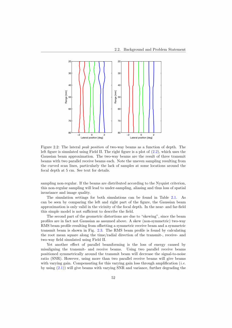
2.2. Background and Problem Statement
−2 0 2
20
30
40
50
60
70
80
Lateral position [deg]
Ran
ge [m
m]
−2 0 2
20
30
40
50
60
70
80
Lateral position [deg]
Ran
ge [m
m]
Figure 2.2: The lateral peak position of two-way beams as a function of depth. Theleft figure is simulated using Field II. The right figure is a plot of (2.2), which uses theGaussian beam approximation. The two-way beams are the result of three transmitbeams with two parallel receive beams each. Note the uneven sampling resulting fromthe curved scan lines, particularly the lack of samples at some locations around thefocal depth at 5 cm. See text for details.
sampling non-regular. If the beams are distributed according to the Nyquist criterion,this non-regular sampling will lead to under-sampling, aliasing and thus loss of spatialinvariance and image quality.
The simulation settings for both simulations can be found in Table 2.1. Ascan be seen by comparing the left and right part of the figure, the Gaussian beamapproximation is only valid in the vicinity of the focal depth. In the near- and far-fieldthis simple model is not sufficient to describe the field.
The second part of the geometric distortions are due to “skewing”, since the beamprofiles are in fact not Gaussian as assumed above. A skew (non-symmetric) two-wayRMS beam profile resulting from offsetting a symmetric receive beam and a symmetrictransmit beam is shown in Fig. 2.3. The RMS beam profile is found by calculatingthe root mean square along the time/radial direction of the transmit-, receive- andtwo-way field simulated using Field II.
Yet another effect of parallel beamforming is the loss of energy caused bymisaligning the transmit- and receive beams. Using two parallel receive beamspositioned symmetrically around the transmit beam will decrease the signal-to-noiseratio (SNR). However, using more than two parallel receive beams will give beamswith varying gain. Compensating for this varying gain loss through amplification (i.e.by using (2.1)) will give beams with varying SNR and variance, further degrading the
52
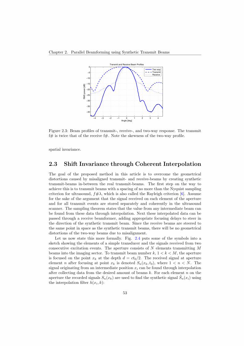
Chapter 2. Parallel Beamforming using Synthetic Transmit Beams
−4 −3 −2 −1 0 1 2 3 4
−40
−35
−30
−25
−20
−15
−10
−5
0
Angle [deg]
RM
S p
ower
[dB
]
Transmit and Receive Beam Profiles
Two wayTransmitReceive
Figure 2.3: Beam profiles of transmit-, receive-, and two-way response. The transmitf# is twice that of the receive f#. Note the skewness of the two-way profile.
spatial invariance.
2.3 Shift Invariance through Coherent Interpolation
The goal of the proposed method in this article is to overcome the geometricaldistortions caused by misaligned transmit- and receive-beams by creating synthetictransmit-beams in-between the real transmit-beams. The first step on the way toachieve this is to transmit beams with a spacing of no more than the Nyquist samplingcriterion for ultrasound, f#λ, which is also called the Rayleigh criterion [6]. Assumefor the sake of the argument that the signal received on each element of the apertureand for all transmit events are stored separately and coherently in the ultrasoundscanner. The sampling theorem states that the value from any intermediate beam canbe found from these data through interpolation. Next these interpolated data can bepassed through a receive beamformer, adding appropriate focusing delays to steer inthe direction of the synthetic transmit beam. Since the receive beams are steered tothe same point in space as the synthetic transmit beams, there will be no geometricaldistortions of the two-way beams due to misalignment.
Let us now state this more formally. Fig. 2.4 puts some of the symbols into asketch showing the elements of a simple transducer and the signals received from twoconsecutive excitation events. The aperture consists of N elements transmitting Mbeams into the imaging sector. To transmit beam number k, 1 < k < M , the apertureis focused on the point xk at the depth d = ct0/2. The received signal at apertureelement n after focusing at point xk is denoted Sn(xk, t0), where 1 < n < N . Thesignal originating from an intermediate position xi can be found through interpolationafter collecting data from the desired amount of beams k. For each element n on theaperture the recorded signals Sn(xk) are used to find the synthetic signal Sn(xi) usingthe interpolation filter h(xi, k):
53
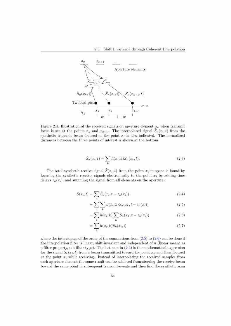
2.3. Shift Invariance through Coherent Interpolation
...
Aperture elements
an an+1
xk
Sn(xk+1, t)
xk+1z
xi
Sn(xk, t)
x
w 1 − w
Tx focal pts.
Sn(xi, t)
Figure 2.4: Illustration of the received signals on aperture element an when transmitfocus is set at the points xk and xk+1. The interpolated signal Sn(xi, t) from thesynthetic transmit beam focused at the point xi is also indicated. The normalizeddistances between the three points of interest is shown at the bottom.
Sn(xi, t) =∑
k
h(xi, k)Sn(xk, t). (2.3)
The total synthetic receive signal S(xi, t) from the point xi in space is found byfocusing the synthetic receive- signals electronically to the point xi by adding timedelays τn(xi), and summing the signal from all elements on the aperture:
S(xi, t) =∑
n
Sn(xi, t − τn(xi)) (2.4)
=∑
n
∑k
h(xi, k)Sn(xk, t − τn(xi)) (2.5)
=∑
k
h(xi, k)∑
n
Sn(xk, t − τn(xi)) (2.6)
=∑
k
h(xi, k)Sk(xi, t) (2.7)
where the interchange of the order of the summations from (2.5) to (2.6) can be done ifthe interpolation filter is linear, shift invariant and independent of n (linear meant asa filter property, not filter type). The last sum in (2.6) is the mathematical expressionfor the signal Sk(xi, t) from a beam transmitted toward the point xk and then focusedat the point xi while receiving. Instead of interpolating the received samples fromeach aperture element the same result can be achieved from steering the receive-beamtoward the same point in subsequent transmit-events and then find the synthetic scan
54
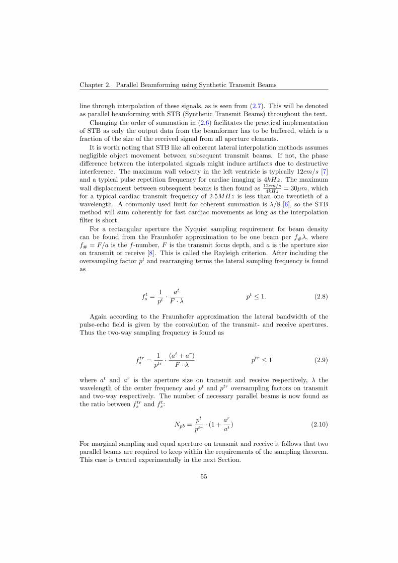
Chapter 2. Parallel Beamforming using Synthetic Transmit Beams
line through interpolation of these signals, as is seen from (2.7). This will be denotedas parallel beamforming with STB (Synthetic Transmit Beams) throughout the text.
Changing the order of summation in (2.6) facilitates the practical implementationof STB as only the output data from the beamformer has to be buffered, which is afraction of the size of the received signal from all aperture elements.
It is worth noting that STB like all coherent lateral interpolation methods assumesnegligible object movement between subsequent transmit beams. If not, the phasedifference between the interpolated signals might induce artifacts due to destructiveinterference. The maximum wall velocity in the left ventricle is typically 12cm/s [7]and a typical pulse repetition frequency for cardiac imaging is 4kHz. The maximumwall displacement between subsequent beams is then found as 12cm/s
4kHz = 30μm, whichfor a typical cardiac transmit frequency of 2.5MHz is less than one twentieth of awavelength. A commonly used limit for coherent summation is λ/8 [6], so the STBmethod will sum coherently for fast cardiac movements as long as the interpolationfilter is short.
For a rectangular aperture the Nyquist sampling requirement for beam densitycan be found from the Fraunhofer approximation to be one beam per f#λ, wheref# = F/a is the f -number, F is the transmit focus depth, and a is the aperture sizeon transmit or receive [8]. This is called the Rayleigh criterion. After including theoversampling factor pt and rearranging terms the lateral sampling frequency is foundas
f ts =
1pt
· at
F · λ pt ≤ 1. (2.8)
Again according to the Fraunhofer approximation the lateral bandwidth of thepulse-echo field is given by the convolution of the transmit- and receive apertures.Thus the two-way sampling frequency is found as
f trs =
1ptr
· (at + ar)F · λ ptr ≤ 1 (2.9)
where at and ar is the aperture size on transmit and receive respectively, λ thewavelength of the center frequency and pt and ptr oversampling factors on transmitand two-way respectively. The number of necessary parallel beams is now found asthe ratio between f tr
s and f ts:
Npb =pt
ptr· (1 +
ar
at) (2.10)
For marginal sampling and equal aperture on transmit and receive it follows that twoparallel beams are required to keep within the requirements of the sampling theorem.This case is treated experimentally in the next Section.
55
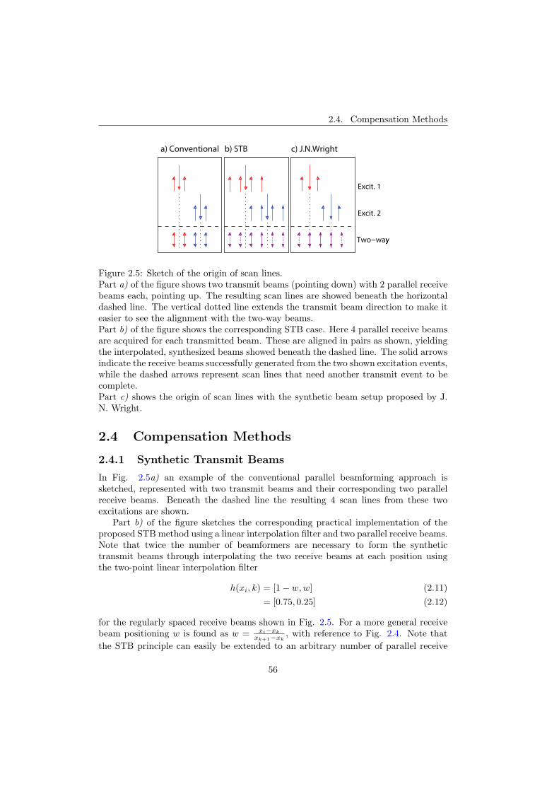
2.4. Compensation Methods
a) Conventional
Excit. 1
Excit. 2
Two−wayy
c) J.N.Wrightb) STB
Figure 2.5: Sketch of the origin of scan lines.Part a) of the figure shows two transmit beams (pointing down) with 2 parallel receivebeams each, pointing up. The resulting scan lines are showed beneath the horizontaldashed line. The vertical dotted line extends the transmit beam direction to make iteasier to see the alignment with the two-way beams.Part b) of the figure shows the corresponding STB case. Here 4 parallel receive beamsare acquired for each transmitted beam. These are aligned in pairs as shown, yieldingthe interpolated, synthesized beams showed beneath the dashed line. The solid arrowsindicate the receive beams successfully generated from the two shown excitation events,while the dashed arrows represent scan lines that need another transmit event to becomplete.Part c) shows the origin of scan lines with the synthetic beam setup proposed by J.N. Wright.
2.4 Compensation Methods
2.4.1 Synthetic Transmit Beams
In Fig. 2.5a) an example of the conventional parallel beamforming approach issketched, represented with two transmit beams and their corresponding two parallelreceive beams. Beneath the dashed line the resulting 4 scan lines from these twoexcitations are shown.
Part b) of the figure sketches the corresponding practical implementation of theproposed STB method using a linear interpolation filter and two parallel receive beams.Note that twice the number of beamformers are necessary to form the synthetictransmit beams through interpolating the two receive beams at each position usingthe two-point linear interpolation filter
h(xi, k) = [1 − w, w] (2.11)= [0.75, 0.25] (2.12)
for the regularly spaced receive beams shown in Fig. 2.5. For a more general receivebeam positioning w is found as w = xi−xk
xk+1−xk, with reference to Fig. 2.4. Note that
the STB principle can easily be extended to an arbitrary number of parallel receive
56

Chapter 2. Parallel Beamforming using Synthetic Transmit Beams
beams, only limited by the number of available receive beamformers.Choosing a linear interpolation filter is the simplest implementation of STB, as
only two receive beams has to be steered toward each desired scan line position. Theimpulse response of the linear interpolation filter is triangular, making it a sinc2-function in the frequency domain [9]. This means that some of the high-frequencycontent of the signal will be attenuated, and there will be some noise due to aliasingfrom the wide transition band. The maximum error will appear for a marginallysampled white-noise process, where the reduction of power without aliasing comparedto ideal interpolation is found from
Perr = 20 log10
⎛⎜⎝
fs/2∫−fs/2
(sin(πf/fs)
πf/fs
)2
df
⎞⎟⎠ = −2.2dB (2.13)
where fs is the sampling frequency and f is the lateral frequency variable.The error will be lower for a band-limited signal, and is further reduced with
oversampling, that is, using a higher density of transmit beams. However this is notwanted as the purpose of parallel beam processing is to obtain a high frame rate, whichnecessitates as scarce positioning of transmit beams as possible.
Higher order interpolation can be used if the necessary number of beamformersare available. Each scan line requires the same number of beamformers as the numberof taps in the interpolation filter. Using an ideal interpolation filter in (2.7) will giveperfect reconstruction with no artifacts from parallel processing. Unfortunately thisrequires an infinitely long interpolation filter, and the same number of beamformers.
2.4.2 Dynamic steering
Most modern (digital) beamformers are using different focusing delays for each depthwhen receiving, ensuring appropriate geometrical focus. This is called dynamicfocusing. If the beamformer also updates the steering delays for each depth, thisis called dynamic steering. Such a beamformer can focus along any line - straight orcurved, upon reception.
If the beamformer is capable of such dynamic steering, another intuitive way ofcompensating for the warping effect is by deliberately offsetting the receive-directionfor each depth in the opposite direction of the warping [10]. To make this work wella reasonably accurate beam model must run on the scanner. From Fig. 2.2 it can beseen that the Gaussian model presented in Section 2.2 can serve this purpose close tothe focal depth, where it can be argued that a good image is most important. In otherwords, offsetting the receive focal direction with the inverse of (2.2) should reducewarping artifacts significantly.
If dynamic steering is not available, a fixed steering offset can be applied toeliminate warping at a desired depth, often chosen as the focal depth. However, thisapproach might lead to poor performance at other depths.
57
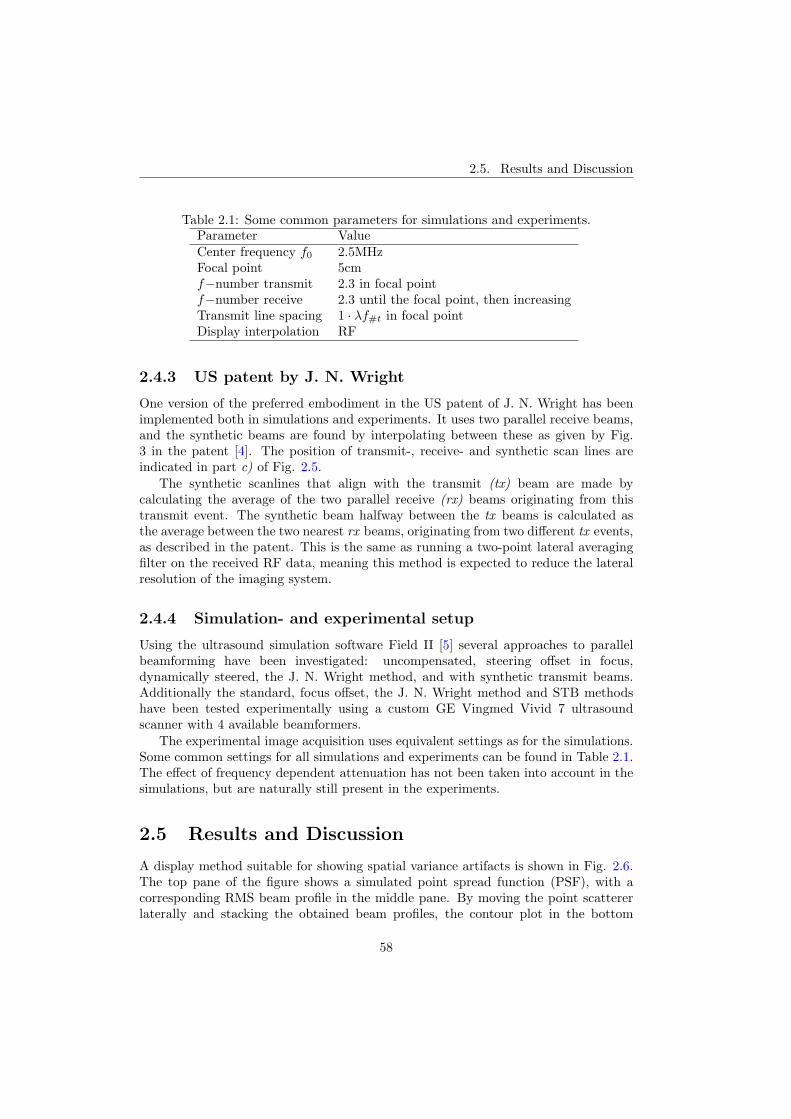
2.5. Results and Discussion
Table 2.1: Some common parameters for simulations and experiments.Parameter ValueCenter frequency f0 2.5MHzFocal point 5cmf−number transmit 2.3 in focal pointf−number receive 2.3 until the focal point, then increasingTransmit line spacing 1 · λf#t in focal pointDisplay interpolation RF
2.4.3 US patent by J. N. Wright
One version of the preferred embodiment in the US patent of J. N. Wright has beenimplemented both in simulations and experiments. It uses two parallel receive beams,and the synthetic beams are found by interpolating between these as given by Fig.3 in the patent [4]. The position of transmit-, receive- and synthetic scan lines areindicated in part c) of Fig. 2.5.
The synthetic scanlines that align with the transmit (tx) beam are made bycalculating the average of the two parallel receive (rx) beams originating from thistransmit event. The synthetic beam halfway between the tx beams is calculated asthe average between the two nearest rx beams, originating from two different tx events,as described in the patent. This is the same as running a two-point lateral averagingfilter on the received RF data, meaning this method is expected to reduce the lateralresolution of the imaging system.
2.4.4 Simulation- and experimental setup
Using the ultrasound simulation software Field II [5] several approaches to parallelbeamforming have been investigated: uncompensated, steering offset in focus,dynamically steered, the J. N. Wright method, and with synthetic transmit beams.Additionally the standard, focus offset, the J. N. Wright method and STB methodshave been tested experimentally using a custom GE Vingmed Vivid 7 ultrasoundscanner with 4 available beamformers.
The experimental image acquisition uses equivalent settings as for the simulations.Some common settings for all simulations and experiments can be found in Table 2.1.The effect of frequency dependent attenuation has not been taken into account in thesimulations, but are naturally still present in the experiments.
2.5 Results and Discussion
A display method suitable for showing spatial variance artifacts is shown in Fig. 2.6.The top pane of the figure shows a simulated point spread function (PSF), with acorresponding RMS beam profile in the middle pane. By moving the point scattererlaterally and stacking the obtained beam profiles, the contour plot in the bottom
58
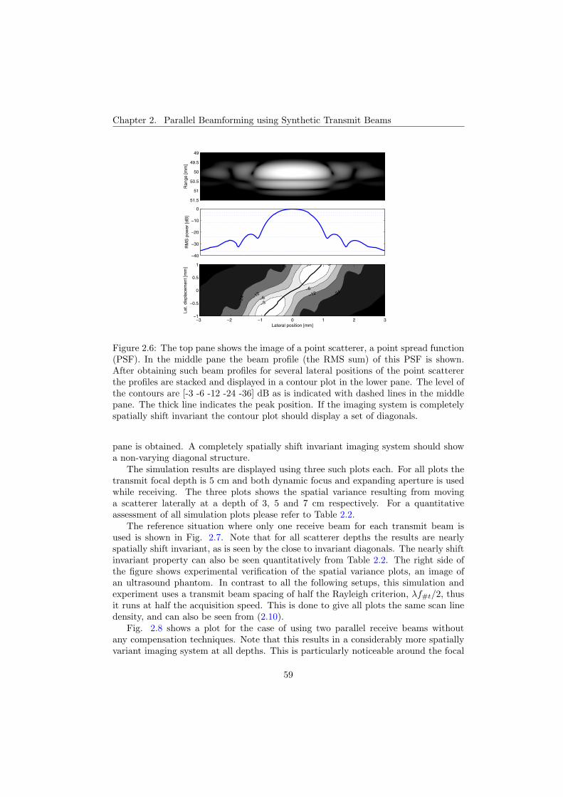
Chapter 2. Parallel Beamforming using Synthetic Transmit Beams
Ran
ge [m
m]
49
49.5
50
50.5
51
51.5
−40
−30
−20
−10
0
RM
S p
ower
[dB
]
−36
−36
−24
−24
−24−12 −12
−6
−6
3
−3
−3
Lateral position [mm]
Lat.
disp
lace
men
t [m
m]
−3 −2 −1 0 1 2 3−1
−0.5
0
0.5
1
Figure 2.6: The top pane shows the image of a point scatterer, a point spread function(PSF). In the middle pane the beam profile (the RMS sum) of this PSF is shown.After obtaining such beam profiles for several lateral positions of the point scattererthe profiles are stacked and displayed in a contour plot in the lower pane. The level ofthe contours are [-3 -6 -12 -24 -36] dB as is indicated with dashed lines in the middlepane. The thick line indicates the peak position. If the imaging system is completelyspatially shift invariant the contour plot should display a set of diagonals.
pane is obtained. A completely spatially shift invariant imaging system should showa non-varying diagonal structure.
The simulation results are displayed using three such plots each. For all plots thetransmit focal depth is 5 cm and both dynamic focus and expanding aperture is usedwhile receiving. The three plots shows the spatial variance resulting from movinga scatterer laterally at a depth of 3, 5 and 7 cm respectively. For a quantitativeassessment of all simulation plots please refer to Table 2.2.
The reference situation where only one receive beam for each transmit beam isused is shown in Fig. 2.7. Note that for all scatterer depths the results are nearlyspatially shift invariant, as is seen by the close to invariant diagonals. The nearly shiftinvariant property can also be seen quantitatively from Table 2.2. The right side ofthe figure shows experimental verification of the spatial variance plots, an image ofan ultrasound phantom. In contrast to all the following setups, this simulation andexperiment uses a transmit beam spacing of half the Rayleigh criterion, λf#t/2, thusit runs at half the acquisition speed. This is done to give all plots the same scan linedensity, and can also be seen from (2.10).
Fig. 2.8 shows a plot for the case of using two parallel receive beams withoutany compensation techniques. Note that this results in a considerably more spatiallyvariant imaging system at all depths. This is particularly noticeable around the focal
59
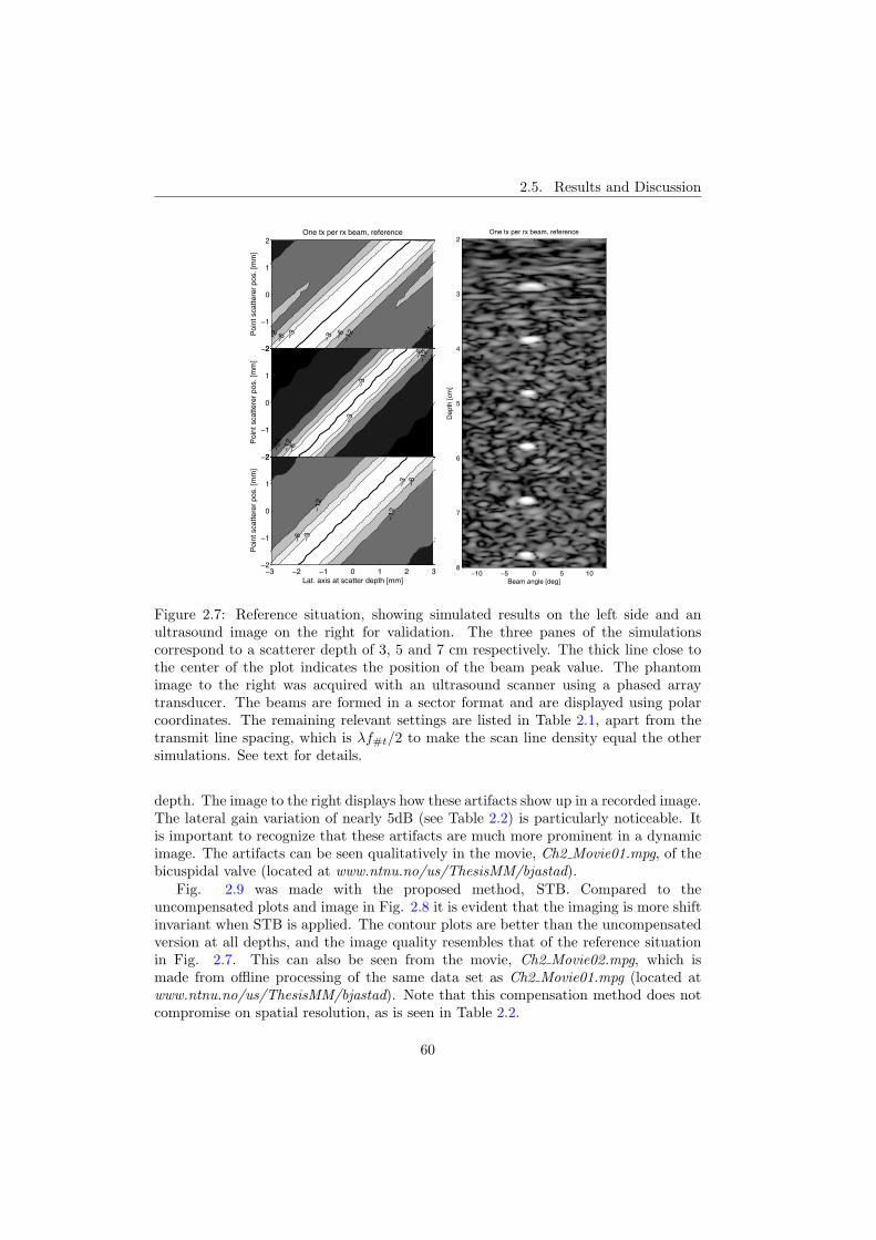
2.5. Results and Discussion
−24
12 −12
−6 −6−3 −3
Poi
nt s
catte
rer
pos.
[mm
]
One tx per rx beam, reference
−2
−1
0
1
2
−24
−24
−12
−12
−6
−6
−3
−3
Poi
nt s
catte
rer
pos.
[mm
]
−2
−1
0
1
2
−12
−12
−6
−6
−3
−3
Lat. axis at scatter depth [mm]
Poi
nt s
catte
rer
pos.
[mm
]
−3 −2 −1 0 1 2 3−2
−1
0
1
2
Beam angle [deg]
Dep
th [c
m]
One tx per rx beam, reference
−10 −5 0 5 10
2
3
4
5
6
7
8
Figure 2.7: Reference situation, showing simulated results on the left side and anultrasound image on the right for validation. The three panes of the simulationscorrespond to a scatterer depth of 3, 5 and 7 cm respectively. The thick line close tothe center of the plot indicates the position of the beam peak value. The phantomimage to the right was acquired with an ultrasound scanner using a phased arraytransducer. The beams are formed in a sector format and are displayed using polarcoordinates. The remaining relevant settings are listed in Table 2.1, apart from thetransmit line spacing, which is λf#t/2 to make the scan line density equal the othersimulations. See text for details.
depth. The image to the right displays how these artifacts show up in a recorded image.The lateral gain variation of nearly 5dB (see Table 2.2) is particularly noticeable. Itis important to recognize that these artifacts are much more prominent in a dynamicimage. The artifacts can be seen qualitatively in the movie, Ch2 Movie01.mpg, of thebicuspidal valve (located at www.ntnu.no/us/ThesisMM/bjastad).
Fig. 2.9 was made with the proposed method, STB. Compared to theuncompensated plots and image in Fig. 2.8 it is evident that the imaging is more shiftinvariant when STB is applied. The contour plots are better than the uncompensatedversion at all depths, and the image quality resembles that of the reference situationin Fig. 2.7. This can also be seen from the movie, Ch2 Movie02.mpg, which ismade from offline processing of the same data set as Ch2 Movie01.mpg (located atwww.ntnu.no/us/ThesisMM/bjastad). Note that this compensation method does notcompromise on spatial resolution, as is seen in Table 2.2.
60

Chapter 2. Parallel Beamforming using Synthetic Transmit Beams
−24
−12
−12
−12
−6
−6
−6
−3 −3
−12
−12
−12
−12
Poi
nt s
catte
rer
pos.
[mm
]
2 parallel beams, uncompensated
−2
−1
0
1
2
−36
−36
−24 −24
−12
−12
−6 −6
−3
−3
−3
−3
Poi
nt s
catte
rer
pos.
[mm
]
−2
−1
0
1
2
−24
−12
−12
−6−6−3
−3
Lat. axis at scatter depth [mm]
Poi
nt s
catte
rer
pos.
[mm
]
−3 −2 −1 0 1 2 3−2
−1
0
1
2
Beam angle [deg]
Dep
th [c
m]
2 parallel beams, uncompensated
−10 −5 0 5 10
2
3
4
5
6
7
8
Figure 2.8: Imaging using 2 parallel receive beams, without any type of compensation.Note the evident lack of spatial invariance, especially with the scatterer at the focaldepth (middle pane). This can also be seen from the ultrasound image to the right,where vertical stripes are apparent in a region around the focal depth of 5 cm.
The method proposed by J. N. Wright was found to perform best when the rx -beams were shifted further away from the tx direction, in the same manner as tocompensate for the warping effect at the focal depth, as described in the section onDynamic steering. The additional shift corresponded to a fourth of the receive linespacing. Results from simulations and experiments with these settings are displayedin Fig. 2.10, and numerical results from the simulations can be found in Table 2.2.Comparing these figures with those of the STB method in Fig. 2.9, the J. N. Wrightmethod is seen to display nearly as good spatial shift invariance as the STB method.However, from the numerical results this method it is seen to give a 15% reduction inlateral resolution when compared to the STB method.
If dynamic steering is not available, the warping can only be fully compensated forat one specific depth. Figure 2.11 shows the results from warp-compensating at thefocal depth. The middle left pane shows that offsetting the steering angle to eliminatewarping at the focal depth successfully eliminates warping in focus. However thespatial invariance is significantly reduced below and above the focal point.
The left pane of Fig. 2.12 shows simulated results from using dynamic steeringto compensate for warping at all depths. Unfortunately no experimental results are
61

2.5. Results and Discussion
24
−24
−12 −12
−6
−6
−6
−3
−3
−3
Poi
nt s
catte
rer
pos.
[mm
]
2 parallel beams with STB
−2
−1
0
1
2
−36
−36
−36
−24
−24
−12
−12
−6
−6
−3
−3
−3Poi
nt s
catte
rer
pos.
[mm
]
−2
−1
0
1
2
−12
−12
−6 −6−3 −3
Lat. axis at scatter depth [mm]
Poi
nt s
catte
rer
pos.
[mm
]
−3 −2 −1 0 1 2 3−2
−1
0
1
2
Beam angle [deg]
Dep
th [c
m]
2 parallel beams with STB
−10 −5 0 5 10
2
3
4
5
6
7
8
Figure 2.9: Much of the artifacts originating from parallel receive beams can beeliminated by using STB imaging, as is shown here. Note the difference from theuncompensated images in Fig. 2.8. Both experimental images were made with thesame parameters and the same transmit- and scan line density. They differ only inthe number of beamformers used. The axes show depth and angle increment, wherethe center line is chosen as zero degrees. Note how the STB image shows no signs ofthe easily noticeable vertical stripes of the image without STB. Also note that thereis still some ripple left at the focal depth of the contour plot. This is probably causedby the non-ideal linear interpolation filter used.
available due to limitations in the available ultrasound scanner. When the steeringcompensation is done dynamically, warping is eliminated at all depths up until theaccuracy of the Gaussian beam approximation. Note that the skewing artifact is leftuncompensated with this approach. This is particularly noticeable in the top panewhere the spatial invariance is poor despite the steering compensation efforts.
For completeness the right pane of Fig. 2.12 shows the simplest option when itcomes to increasing the acquisition rate, simply decreasing the scan line density. Fromthe two bottom panes it is seen that this approach suffers from under-sampling. Itimportant to remember that the sampling criterion has to be credited at both transmit,receive and two-way. Even if this simple method has sufficient sampling on transmitand receive, the two-way situation is under-sampled.
Some numerical results from the simulation study are summarized in Table 2.2.
62

Chapter 2. Parallel Beamforming using Synthetic Transmit Beams
4
−24
−24
12
−12
−12
−12−6
−6 −6
−6
−3
−3
−3
−3
Poi
nt s
catte
rer
pos.
[mm
]
2 parallel beams, JNWright with offset
−2
−1
0
1
2
−36
−36
−24−24
−24
−12
−12
−12
−6
−6 −6
−6−3
−3 −3
−3 −36
−36
−36
−36
−36
6
Poi
nt s
catte
rer
pos.
[mm
]
−2
−1
0
1
2
24
−24
−24
−12 −12
−126
−6
−6
−6−3
−3
−3
−3
Lat. axis at scatter depth [mm]
Poi
nt s
catte
rer
pos.
[mm
]
−3 −2 −1 0 1 2 3−2
−1
0
1
2
Beam angle [deg]
Dep
th [c
m]
Compensation method of J. N. Wright.
−10 −5 0 5 10
2
3
4
5
6
7
8
Figure 2.10: The J. N. Wright method with a static receive beam offset. No easilynoticeable vertical stripes can be seen in the image. The image is however more blurredthan the corresponding STB image. Also notice the more variable peak position (thicksolid line) at all depths compared to STB.
The results of the first two columns are calculated with normalized beams, that is,the peak value is zero for all lateral scatter positions. The first column lists themean -6dB beam width. The “Width var.” and “Gain var.” columns quantifies thedifference between the min. and max. -6dB beam width and the peak gain differencerespectively. The “Offset” column is computed to give a measure of the meanderingmovement of the peak position. It is given as the ratio of the two-sided lateral peakposition error and the mean beam width at each depth.
Investigating the first column of the Table, it is seen that the mean beam width ofthe J. N. Wright method is slightly larger than for the other imaging methods. This canbe contributed to the lateral filtering performed in this method. Apart from that, themean beam width at at each depth is quite constant for each imaging method, with theexception of the undersampled method. Note that this is the case even when steeringcompensation methods are applied. Using a Gaussian beam profile approximation itcan easily be shown that this is as expected. Looking at mean beam widths does nottell anything about the shift invariance property of the methods. This is better seen inthe next column, displaying the difference between the maximum and minimum beamwidth as the scatterer is moved laterally. It can here be observed that all methods,
63

2.5. Results and Discussion
Table 2.2: Numerical results from comparison of parallel beamforming techniques.
Method Depth
Meanbeamwidth[mm]
Width var.Gainvar.[dB]
Offset
Reference,30 mm 2 3% 0.3 2%50 mm 1.2 15% 0.64 11%70 mm 2.1 7% 0.32 5%
Uncomp.,30 mm 2 5% 0.32 11%50 mm 1.3 37% 4.8 29%70 mm 2.1 18% 1.4 13%
Focus comp.,30 mm 2.1 76% 0.89 50%50 mm 1.2 13% 0.76 12%70 mm 2.3 115% 3.66 48%
Dyn. steered,30 mm 2 4% 0.48 15%50 mm 1.2 13% 0.72 11%70 mm 2.1 12% 0.92 9%
STB,30 mm 1.9 2% 0.29 6%50 mm 1.3 16% 1.97 16%70 mm 2.1 10% 0.79 6%
J.N.Wright method,30 mm 2 7% 0.91 23%50 mm 1.5 15% 2.12 16%70 mm 2.4 18% 1.06 13%
Undersampled,30 mm 2.2 25% 0.51 9%50 mm 1.6 86% 7.09 89%70 mm 2.6 57% 3.49 41%
except for the focus compensation method, perform best before and after the focaldepth. This is due to the wider transmit beam at these depths. At the focal depththe -6dB beam width vary with 37% when no compensation is done. When applyingeither dynamic steering, the J. N. Wright method, or STB, all of which have similarperformance here, the width variation is greatly reduced to around 15%, the same as inthe reference situation. Looking at the next column, the gain variation, the dynamicsteering method performs best, reducing the variation from 4.88dB uncompensatedto 0.72dB at focal depth. That is only slightly higher than the reference situationand then as good as one can expect it to be with the applied beam density. Aninteresting number is the 2dB gain variation at the focal depth for the STB method.
64
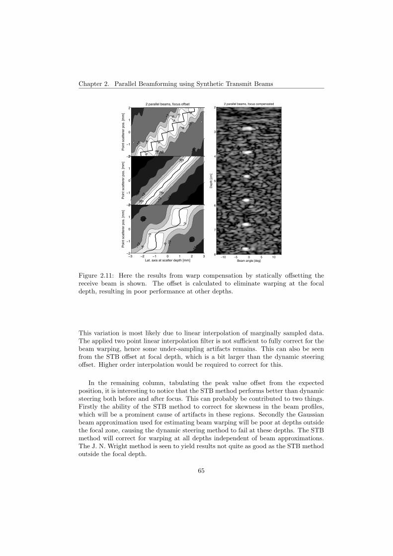
Chapter 2. Parallel Beamforming using Synthetic Transmit Beams
−24
−12
−12
−12
−12
−6
−6
−6
−6−3
−3
−3
−3
−3
−3
Poi
nt s
catte
rer
pos.
[mm
]
2 parallel beams, focus offset
−2
−1
0
1
2
−36
−24
−24−1
2
−12
−6
−6
−6
−3
−3
−3
Poi
nt s
catte
rer
pos.
[mm
]
−2
−1
0
1
2
−24−1
2 −12
−6
−6
−3
−3 −24
−24
Lat. axis at scatter depth [mm]
Poi
nt s
catte
rer
pos.
[mm
]
−3 −2 −1 0 1 2 3−2
−1
0
1
2
Beam angle [deg]
Dep
th [c
m]
2 parallel beams, focus compensated
−10 −5 0 5 10
2
3
4
5
6
7
8
Figure 2.11: Here the results from warp compensation by statically offsetting thereceive beam is shown. The offset is calculated to eliminate warping at the focaldepth, resulting in poor performance at other depths.
This variation is most likely due to linear interpolation of marginally sampled data.The applied two point linear interpolation filter is not sufficient to fully correct for thebeam warping, hence some under-sampling artifacts remains. This can also be seenfrom the STB offset at focal depth, which is a bit larger than the dynamic steeringoffset. Higher order interpolation would be required to correct for this.
In the remaining column, tabulating the peak value offset from the expectedposition, it is interesting to notice that the STB method performs better than dynamicsteering both before and after focus. This can probably be contributed to two things.Firstly the ability of the STB method to correct for skewness in the beam profiles,which will be a prominent cause of artifacts in these regions. Secondly the Gaussianbeam approximation used for estimating beam warping will be poor at depths outsidethe focal zone, causing the dynamic steering method to fail at these depths. The STBmethod will correct for warping at all depths independent of beam approximations.The J. N. Wright method is seen to yield results not quite as good as the STB methodoutside the focal depth.
65
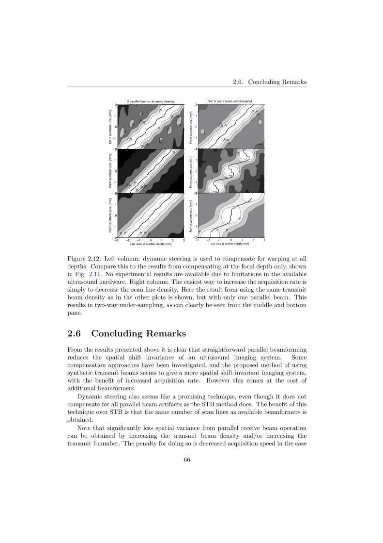
2.6. Concluding Remarks
−24
−24
−12
−12
−12
−6
−6
−6
−3
−3
−3−12
−12
−12−1
2
−12
−12
Poi
nt s
catte
rer
pos.
[mm
]
2 parallel beams, dynamic steering
−2
−1
0
1
2
−36
−36
−24
−24
−12
−12−6 −6
−3
−3
−3
Poi
nt s
catte
rer
pos.
[mm
]
−2
−1
0
1
2
−24
24
2
−12
−6 −6−3 −3
Lat. axis at scatter depth [mm]
Poi
nt s
catte
rer
pos.
[mm
]
−3 −2 −1 0 1 2 3−2
−1
0
1
224
−24
−12
−12
−12
−6
−6
−6
−3
−3
−3
−12
−12
Poin
t sca
tter
er p
os. [
mm
]
One tx per rx beam, undersampled
−2
−1
0
1
2
6
4
−24
−24
−24
−12
−12
−12
−6
−6
−3
−3
−3Po
int s
catt
erer
pos
. [m
m]
−2
−1
0
1
2
2
−12−6
−6
−3
−3
−3
Lat. axis at scatter depth [mm]
Poin
t sca
tter
er p
os. [
mm
]
−3 −2 −1 0 1 2 3−2
−1
0
1
2
Figure 2.12: Left column: dynamic steering is used to compensate for warping at alldepths. Compare this to the results from compensating at the focal depth only, shownin Fig. 2.11. No experimental results are available due to limitations in the availableultrasound hardware. Right column: The easiest way to increase the acquisition rate issimply to decrease the scan line density. Here the result from using the same transmitbeam density as in the other plots is shown, but with only one parallel beam. Thisresults in two-way under-sampling, as can clearly be seen from the middle and bottompane.
2.6 Concluding Remarks
From the results presented above it is clear that straightforward parallel beamformingreduces the spatial shift invariance of an ultrasound imaging system. Somecompensation approaches have been investigated, and the proposed method of usingsynthetic transmit beams seems to give a more spatial shift invariant imaging system,with the benefit of increased acquisition rate. However this comes at the cost ofadditional beamformers.
Dynamic steering also seems like a promising technique, even though it does notcompensate for all parallel beam artifacts as the STB method does. The benefit of thistechnique over STB is that the same number of scan lines as available beamformers isobtained.
Note that significantly less spatial variance from parallel receive beam operationcan be obtained by increasing the transmit beam density and/or increasing thetransmit f-number. The penalty for doing so is decreased acquisition speed in the case
66

Chapter 2. Parallel Beamforming using Synthetic Transmit Beams
of increased transmit beam density. The main drawback of increasing the transmit f-number is reduced penetration. Additionally it will give a wider transmit focus, givingpoorer resolution.
It is worth noting that different underlying phenomena contribute to the artifactsat increasing depth. In the region close to the transducer the skewing effect is thedominant artifact. In the focal region the warping effect dominates, while deeper inthe image both effects contribute.
67

2.6. Concluding Remarks
68
References
[1] O. T. von Ramm, S. W. Smith, and H. G. Pavy, “High-speed ultrasoundvolumetric imaging system – part ii: Parallel processing and image display,”IEEE transactions on ultrasonics, ferroelectrics, and frequency control, vol. 38,March 1991.
[2] D. P. Shattuck, M. D. Weinshenker, S. W. Smith, and O. T. von Ramm,“Explososcan: A parallel processing technique for high speed ultrasound imagingwith linear phased arrays,” J. Acoust, Soc. Amer., vol. 75, no. 4, pp. 1273–1282,1984.
[3] L. J. Augustine, High resolution multiline ultrasonic beamformer. United StatesPatent 4.644.795, 1987.
[4] N. Wright et al., Method and apparatus for coherent image formation. UnitedStates Patent 5.623.928, 1997.
[5] J. A. Jensen, “Field: A program for simulating ultrasound systems,” Medical &Biological Engineering & Computing, 1996.
[6] J. N. Wright, Image formation in diagnostic ultrasound. IEEE internationalultrasonics symposium short course, 1997.
[7] M. Kowa�lski, T. Kukulski, F. Jamal, J. D’Hooge, F. Weidemann, F. Rademakers,B. Bijnens, L. Hatle, and G. R. Sutherland, “Can natural strain and strainrate quantify regional myocardial deformation? a study in healthy subjects,”Ultrasound in Med. & Biol., vol. 27, no. 8, pp. 1087–1097, 2001.
[8] T. L. Szabo, Diagnostic ultrasound imaging inside out. Elsevier academic press,2004.
[9] J. G. Proakis and D. G. Manolakis, Digital Signal Processing. Principles,Algorithms, and Applications. London: Prentice Hall, third ed., 1996.
[10] K. E. Thiele and A. Brauch, Method and apparatus for dynamically steeringultrasonic phased arrays. United States Patent 5.322.068, 1994.
69

References
70
Chapter 3
The Impact of Aberration onHigh Frame Rate CardiacB-Mode ImagingT. Bjastad and S. A. Aase, and H. TorpDept. Circulation and Medical Imaging, NTNU
In echocardiography, especially in 3D echocardiography, achieving highframe rates is a major challenge. A suggested solution is parallel receivebeamforming. Without any compensation, this approach is known to produceblock-like artifacts, where each block corresponds to one parallel receive group.In this work, in vitro imaging, in vivo imaging, and simulations were used toinvestigate the artifacts. In vitro, imaging a tissue phantom, the artifactswere successfully compensated for. However, in vivo, imaging the heart, thecompensation techniques no longer sufficed and the artifacts persisted. Within vivo imaging, aberrating tissue layers are present between the heart and theprobe. To investigate the effects of aberration on a parallel receive system, anin vitro experiment was performed with and without a silicon phase aberratorin front of the probe. The aberrator caused the artifacts to appear even whencompensation techniques were applied. Simulations confirmed the measuredresults and indicated that distorted beam profiles and decorrelation betweenparallel receive groups caused the artifacts. To quantify the magnitude ofthe artifacts, a correlation-based indicator was developed. The indicatorseparated images with and without artifacts and confirmed that the artifactsappeared from the combination of parallel receive beams and aberration.
3.1 Introduction
To study deformation in all phases of the cardiac cycle, sufficient temporal resolution,frame rate, is needed. Using 3D ultrasound, far more data have to be recorded in thesame amount of time, thus making it more challenging to achieve a high frame rate.
To achieve high frame rates and still keep sufficient spatial resolution, parallel
71
3.1. Introduction
receive beams can be applied [1, 2]. Using parallel receive beams, multiple scanlines are acquired for each transmit event, hence increasing the frame rate. Parallelbeamforming is therefore also known as multiple line acquisition (MLA). As describedin [3–5] this technique has some challenges due to misalignment of the transmit andreceive beams. If not compensated for, this causes block-like artifacts in the B-modeimages and also a periodical lateral gain variation pattern. These effects will bereferred to as MLA artifacts.
Several compensation methods have been proposed. In U.S. patents [3] and [6], theauthors describe incoherent methods for beam interpolation applied after detection ofthe RF signal. These methods take nonuniform lateral distribution of two-way beamprofiles and gain variation into account. In [4], coherent interpolation is used to producesynthetic scan lines in between the original ones, taking advantage of the fact that thelateral bandwidth increases in the detection step. This increases the beam density andthereby reduces the required number of MLA channels. Another method for MLAcorrection is described in [5], where synthetic transmit beams are generated in thedirection of each receive beam by interpolating the RF-signal from each transducerelement prior to receive beamforming. Coherent interpolation between scan lines fromdifferent transmit pulses is sensitive to rapid motion. This limits the applicability ofthe two latter methods in cardiac imaging. A solution with dynamic beam steeringis suggested in [7]. In this solution the receive focusing is steered dynamically inthe lateral direction to compensate for the nonuniform lateral distribution of two-waybeam profiles.
When imaging the heart, the transmit and receive beams of an ultrasound systemwill be distorted due to inhomogeneities in the body wall. This phenomenon is knownas aberration. MLA systems require a specific geometric relation between the transmitand receive beams. Since aberration distorts the beams, it is likely that aberrationwill have an effect on the ability to correct for MLA artifacts.
We show that cardiac in vivo MLA images contain block artifacts even whenbeam steering and gain compensation techniques are used. A major differencebetween in vitro images, where compensation is successful, and cardiac images, wherecompensation fails, is aberration. In this paper we therefore investigate the impact ofaberration on MLA imaging systems, suggesting that aberration is a major reason forfailing compensation in cardiac MLA images.
The outline of this investigation is as follows: First, the artifacts of MLA areexplained and demonstrated in vivo. Having established the problem, it is shown thatthese artifacts can be corrected when imaging a tissue mimicking phantom where noaberration is present. When placing a thin silicon aberrator between the probe andphantom, it is shown that the compensation techniques no longer suffice. Further,the effects and mechanisms of aberration in conjunction with MLA are investigatedthrough simulations and correlation analysis.
72

Chapter 3. Aberration and High Frame Rate B-mode Imaging
3.2 Theory
3.2.1 Multi-Line Acquisition
The transmit and receive directions of an MLA setup are illustrated in Fig. 3.1. Thinlines indicate receive directions and thick lines the transmit directions. Several receivescan lines are formed in parallel for each transmit event and constitute an MLA group.An MLA system with four parallel receive lines in each MLA group will be referred toas a 4MLA system.
Figure 3.1: 4MLA ultrasound scan grid with Tx lines (thick) and Rx lines (thin).Magnified section: Part of ultrasound scan grid with visualization of MLA groups andscan line correlation pairs.
As described in [5], MLA image artifacts are caused by the misalignment of thetransmit and receive beams. The misalignment pulls the lateral maximum of the two-way beam profiles toward the transmit beam lateral maximum. This causes irregularoverlaps between adjacent two-way beam profiles. If not compensated for, there willbe a gap in the sampling between the MLA groups and hence irregular sampling. Thiseffect is referred to as warping and causes sharp lateral discontinuities in the image.The discontinuities can be seen as the edges of the block artifacts in the images. Asproposed by [7], this warping can be compensated for by steering the receive beamsan appropriate amount away from the transmit beam. This will result in more regularlateral sampling. Since the warping effect varies with depth, this steering shouldideally be dynamic. However, a static steering offset will be sufficient as long as thebeam widths of the transmit and receive beams are constant over the relevant depthrange.
73
3.2. Theory
Another effect of the transmit-receive misalignment is that the shape of the beamprofiles is asymmetric and changes from beam to beam within an MLA group. Thevariation in shape will result in a variation in overlap between adjacent two way beamprofiles. This effect is referred to as skewing.
A third effect is that the outermost two-way beams in a 4MLA group have a lowersensitivity than the innermost. This causes a periodical lateral gain variation patternin the image. The lateral gain variation pattern can be compensated for based eitheron a priori knowledge of the transmit and receive beams or on the measured gainvariations in the recording. In the first approach, based on a priori knowledge, thegain compensation can be found by integrating two-way beam profiles. Estimating thegain variations from the recordings can be done in several ways. A straight forwardtechnique is to calculate the relative gain variations internally in each MLA group.Averaging these internal variations for MLA groups in all positions, depths and frameswill give a set of gain compensation values relatively independent of the imaged object.This method produces a number of gain compensation values equal to the size of anMLA group. A prerequisite for using only these compensation values is that the gainvariations be constant throughout the image. This again requires the transmit andreceive beam width to be constant. This will in most cases only be valid in a limitedarea (roughly equal to the depth of focus).
3.2.2 Correlation Analysis
The most important contributor to MLA artifacts is assumed to be irregular overlapbetween adjacent two way beam profiles. This causes irregular sampling of the imagedobject. With correlation analysis of each pair of adjacent scan lines, the distributionof correlation values will be related to the regularity of the sampling. With regularsampling, all pairs should show similar correlation. In the case of irregular sampling,different pairs will have different correlation. To detect differences in correlation, thecorrelation values of each pair must be compared with the other pairs. A likelihoodratio test can be performed to find sufficient statistic for separating two differentcorrelation values.
Letting X = [x1, x2] where x1 and x2 are complex demodulated RF data from twoadjacent scan lines, and modeling the signal as a zero mean complex Gaussian process,the probability density function is
p(X) = π−2|C|−1eXHC−1X . (3.1)
(From Eq. 15.17 in [8].) Assuming equal variance, σ2, the covariance matrices underhypothesis H0 and H1 are
H0 : C0 = σ2
[1 ρ0
ρ∗0 1
]and
74
Chapter 3. Aberration and High Frame Rate B-mode Imaging
H1 : C1 = σ2
[1 ρ1
ρ∗1 1
],
where ρ0 and ρ1 are different real positive numbers representing two differentnormalized cross correlation factors. H0 could, for instance, represent a pair withhigh cross correlation whereas H1 could represent a pair with low cross correlation.
The likelihood ratio is defined in Eq. 13 in [9] as
Λ(X) =px|H1(X|H1)px|H0(X|H0)
(3.2)
The log likelihood ratio using Eqs. 3.1 and 3.2 reduces to
log(Λ(X)) = b · (R11 + R22) ·(
1 − c · 2Real(R12)R11 + R22
), (3.3)
where b and c are constants given by ρ0 and ρ1 and Rij = 1d
∑n−1r=n−d xi(r)x∗
j (r).The Rij estimate is calculated as correlation between data at scan lines i and j at d
depths given by sample numbers r. When averaging over several depths, R11 and R22
are approximately constant, and the latter part of the expression becomes a sufficientstatistic. The correlation coefficient, being an optimal test for separating two differentcorrelation values, then becomes:
Cc =2Real(Rij)Rii + Rjj
. (3.4)
Due to the normalization, Cc will range from 0, when no correlation is found betweenthe scan lines, to 1, when full correlation is found between the scan lines.
Cc can be calculated for each adjacent pair of scan lines as shown in Fig. 3.1. Tocompensate for gain variation along the scan lines, Cc can be calculated in sectionsalong the scan lines and then averaged. The calculated final Cc for each scan line paircan be visualized in a Cc plot representing all scan line pairs.
Cc values and Cc plots contain information concerning the correlation from scanline to scan line. Of special interest regarding MLA are Cc values at transitionsbetween MLA groups compared to Cc values within MLA groups. To get asingle quantitative measure for this, an indicator of fractional correlation coefficientdifference, Dc, can be calculated as:
Dc =1N
∑ij∈W Cc − 1
M
∑ij∈T Cc
1N
∑ij∈W Cc
· 100, (3.5)
where ij is a pair of adjacent scan lines. The set W contains all such pairs withinMLA groups, and the set T contains all such pairs located at transitions between MLAgroups (such as correlation pair 4 in Fig. 3.1). N is the size of the set W , and M is thesize of the set T . Dc will be 0 when no repeating difference in correlation within and
75

3.3. Setup
Table 3.1: Scan setupTransmit frequency 2.5 MHzReceive frequency 2.5 MHz# receive lines 96Sector width 75 degBeam spacing 0.79 degTransmit aperture width 7.5 mmReceive aperture width Expanding (max: 2.19 cm)Transmit apodization RectangularReceive apodization HammingTransmit focus 70 mmReceive focus Dynamic
between MLA groups is present. When there is full correlation within MLA groupsand no correlation between MLA groups, it will be 100.
3.3 Setup
An M3S probe and a GE Vingmed System 7 scanner capable of recording RF datawas set up with the specifications given in Table 4.1. Using this setup both 4MLAand single line acquisition (SLA) were implemented. The setup was designed to beable to compensate for the negative effects of MLA. Hamming apodization on receivelowers the side lobes. This results in less skewing due to more symmetric two waybeam profiles. The small transmit aperture also reduces the skewing effect due towider transmit beams. In addition, it results in a long focus, hence enabling goodcompensation for the warping and gain variation effect over a long depth range. Thedistribution of transmit and receive scan lines is visualized in Fig. 3.1. The warpcompensation was implemented by steering the inner beams of the MLA groups anadditional 14% of the beam spacing away from the transmit beam directions and theouter beams of the MLA groups an additional 42%. The compensation steering offsetswere found through simulations of the described setup.
The recorded RF data were processed to B-mode display by detection, time gaincompensation, log compression, and scan conversion. A 40-dB dynamic range wasused in the images.
Using the described setup, an ultrasound phantom (CIRS Model 40, GeneralPurpose Multi-Tissue Ultrasound Phantom, 0.5 dB/cm/Mhz; CIRS, Inc., Norfolk,VA) was imaged while tilting the probe from side to side. The left ventricle (LV) ofthe heart of a healthy adult subject was also imaged.
To isolate the effects of aberration, a thin silicon aberrator, described in [10], wasplaced between the probe and the phantom for some recordings. This was a puretime-delay aberrator with a RMS time delay of 48.5 ns. This is similar to RMS timedelays found in [11]. Since the RMS delay value for this aberrator corresponded toan abdominal body wall, a scaled-down version of the aberrator was also tested in
76
Chapter 3. Aberration and High Frame Rate B-mode Imaging
simulations. The RMS delay value of this scaled aberrator was set to 21.1 ns. Thiscorresponds to typical values for thoracic body walls [12]. The correlation lengths ofboth aberrators were also in the range of typical thoracic body walls (2.47 mm) [12].
The described setup, aberrators, CIRS phantom, and a left ventricle computermodel were also simulated in Matlab using Field II [13]. The left ventriclecomputer model is described in [14]. When gain compensation was applied, the gaincompensation values were estimated from the recorded data and applied to the RFdata before further processing.
To produce a quantitative analysis of the images, Cc values between neighboringbeams were calculated (a total of 95 pairs) using data from all frames of the recordings.To emphasize the difference in Cc values between scan lines within MLA groups andbetween groups, every fourth Cc value is colored brighter in the bar plots. Cc analysiswas performed after the data were gain corrected.
Since the gain and warp compensation are valid only throughout the depth of focus,only data from the lower 2/3 part of each image were used when estimating both gaincompensation and Cc values. The extent of this area is illustrated by a gray bar atthe left side of the ultrasound sector in all images.
3.4 Results
All B-mode images in this section are also available as videos. The videos provide afar better impression of the described artifacts than the still images. These will bereferred to with file names and can be found at www.ntnu.no/us/ThesisMM/bjastad.
3.4.1 Measurements
With the described 4MLA setup, a frame rate of 163 frames/s was achieved on thescanner. An image of the left ventricle of a healthy adult subject acquired usingthis setup without warp compensation is shown in Fig. 3.2. Notice the block-likeappearance.
Images of the CIRS phantom are presented in Figs. 3.3 and 3.4. In Fig. 3.3, thephantom was imaged using the 4MLA setup without warp and gain compensation.The block artifacts are observable in the image/video. The Cc plot shows a repeatingpattern of three high Cc values followed by a lower Cc value. In Fig. 3.4, the describedgain and warp compensation has been applied. No lateral block artifacts can be seenin this image, and the repeating pattern of three high Cc values followed by a lowerCc value is not present.
A cardiac ultrasound image with gain and warp compensation using the described4MLA setup is shown in Fig. 3.5. The block artifacts are not as obvious as in Fig.3.2, but they are still visible. When the Cc plot is observed, the repeating pattern ofthree high Cc values followed by a lower Cc value is evident. Using SLA but otherwisethe same setup produced the image in Fig. 3.6. There is no repeating pattern in thecorresponding Cc plot.
77
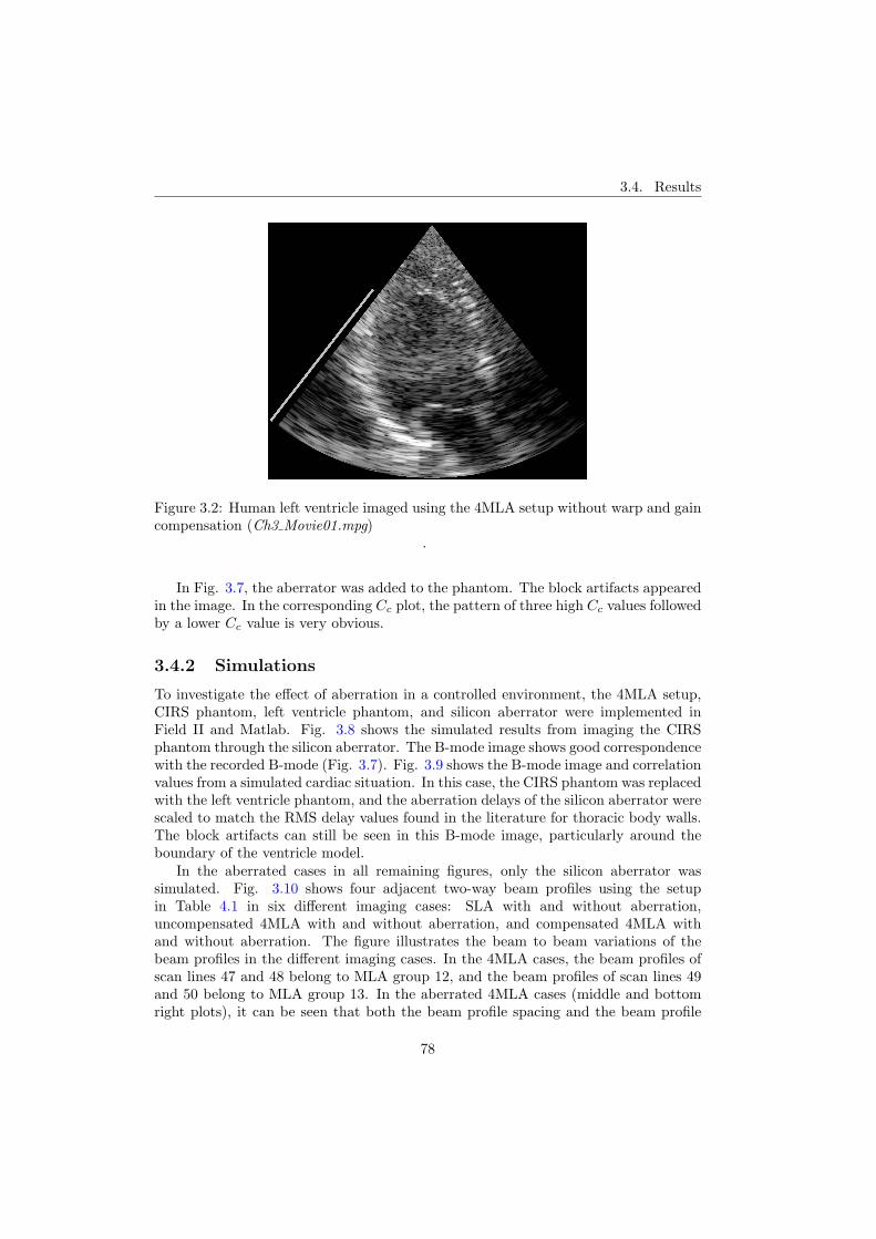
3.4. Results
Figure 3.2: Human left ventricle imaged using the 4MLA setup without warp and gaincompensation (Ch3 Movie01.mpg)
.
In Fig. 3.7, the aberrator was added to the phantom. The block artifacts appearedin the image. In the corresponding Cc plot, the pattern of three high Cc values followedby a lower Cc value is very obvious.
3.4.2 Simulations
To investigate the effect of aberration in a controlled environment, the 4MLA setup,CIRS phantom, left ventricle phantom, and silicon aberrator were implemented inField II and Matlab. Fig. 3.8 shows the simulated results from imaging the CIRSphantom through the silicon aberrator. The B-mode image shows good correspondencewith the recorded B-mode (Fig. 3.7). Fig. 3.9 shows the B-mode image and correlationvalues from a simulated cardiac situation. In this case, the CIRS phantom was replacedwith the left ventricle phantom, and the aberration delays of the silicon aberrator werescaled to match the RMS delay values found in the literature for thoracic body walls.The block artifacts can still be seen in this B-mode image, particularly around theboundary of the ventricle model.
In the aberrated cases in all remaining figures, only the silicon aberrator wassimulated. Fig. 3.10 shows four adjacent two-way beam profiles using the setupin Table 4.1 in six different imaging cases: SLA with and without aberration,uncompensated 4MLA with and without aberration, and compensated 4MLA withand without aberration. The figure illustrates the beam to beam variations of thebeam profiles in the different imaging cases. In the 4MLA cases, the beam profiles ofscan lines 47 and 48 belong to MLA group 12, and the beam profiles of scan lines 49and 50 belong to MLA group 13. In the aberrated 4MLA cases (middle and bottomright plots), it can be seen that both the beam profile spacing and the beam profile
78
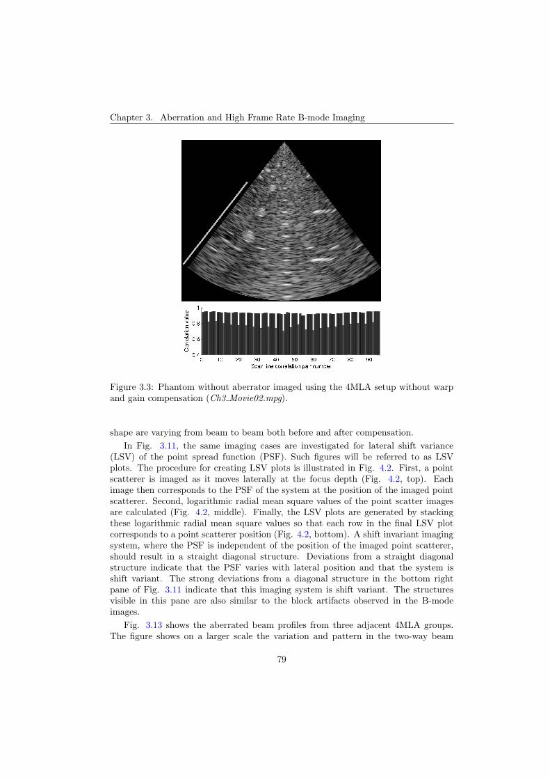
Chapter 3. Aberration and High Frame Rate B-mode Imaging
Figure 3.3: Phantom without aberrator imaged using the 4MLA setup without warpand gain compensation (Ch3 Movie02.mpg).
shape are varying from beam to beam both before and after compensation.In Fig. 3.11, the same imaging cases are investigated for lateral shift variance
(LSV) of the point spread function (PSF). Such figures will be referred to as LSVplots. The procedure for creating LSV plots is illustrated in Fig. 4.2. First, a pointscatterer is imaged as it moves laterally at the focus depth (Fig. 4.2, top). Eachimage then corresponds to the PSF of the system at the position of the imaged pointscatterer. Second, logarithmic radial mean square values of the point scatter imagesare calculated (Fig. 4.2, middle). Finally, the LSV plots are generated by stackingthese logarithmic radial mean square values so that each row in the final LSV plotcorresponds to a point scatterer position (Fig. 4.2, bottom). A shift invariant imagingsystem, where the PSF is independent of the position of the imaged point scatterer,should result in a straight diagonal structure. Deviations from a straight diagonalstructure indicate that the PSF varies with lateral position and that the system isshift variant. The strong deviations from a diagonal structure in the bottom rightpane of Fig. 3.11 indicate that this imaging system is shift variant. The structuresvisible in this pane are also similar to the block artifacts observed in the B-modeimages.
Fig. 3.13 shows the aberrated beam profiles from three adjacent 4MLA groups.The figure shows on a larger scale the variation and pattern in the two-way beam
79
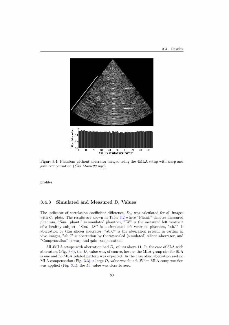
3.4. Results
Figure 3.4: Phantom without aberrator imaged using the 4MLA setup with warp andgain compensation (Ch3 Movie03.mpg).
profiles.
3.4.3 Simulated and Measured Dc Values
The indicator of correlation coefficient difference, Dc, was calculated for all imageswith Cc plots. The results are shown in Table 3.2 where ”Phant.” denotes measuredphantom, ”Sim. phant.” is simulated phantom, ”LV” is the measured left ventricleof a healthy subject, ”Sim. LV” is a simulated left ventricle phantom, ”ab.1” isaberration by thin silicon aberrator, ”ab.C” is the aberration present in cardiac invivo images, ”ab.2” is aberration by thorax-scaled (simulated) silicon aberrator, and”Compensation” is warp and gain compensation.
All 4MLA setups with aberration had Dc values above 11. In the case of SLA withaberration (Fig. 3.6), the Dc value was, of course, low, as the MLA group size for SLAis one and no MLA related pattern was expected. In the case of no aberration and noMLA compensation (Fig. 3.3), a large Dc value was found. When MLA compensationwas applied (Fig. 3.4), the Dc value was close to zero.
80

Chapter 3. Aberration and High Frame Rate B-mode Imaging
Figure 3.5: Human left ventricle imaged using the 4MLA setup with warp and gaincompensation (Ch3 Movie04.mpg).
Table 3.2: Indicator showing differences in correlation, Dc
Object Aberration #MLA Compensation Figure Dc
Phant. 4MLA No 3.3 17.7Phant. 4MLA Yes 3.4 -1.5Phant. ab.1 4MLA Yes 3.7 22.9Sim. phant. ab.1 4MLA Yes 3.8 19.8LV ab.C 4MLA Yes 3.5 17.4LV ab.C SLA 3.6 0.02Sim. LV ab.2 4MLA Yes 3.9 11.6
3.5 Discussion
The cardiac images recorded using 4MLA (Figs. 3.2 and 3.5) showed block artifacts.Although the artifacts were reduced by using warp compensation (Fig. 3.5), they werestill visible.
To first study a simpler situation, a tissue mimicking phantom was used. Theresults showed that block artifacts in unaberrated 4MLA phantom images can beavoided by using warp and gain compensation (Figs. 3.3 and 3.4). The beam profilesin the two lower left panes of Fig. 3.10 correspond to Figs. 3.3 and 3.4, respectively.
81

3.5. Discussion
Figure 3.6: Human left ventricle imaged using the SLA setup (96 transmit beams)(Ch3 Movie05.mpg).
From the beam profiles, it is evident that warping is the main distorting effect. Skewingis not observable.
To emulate aberration, the thin silicon aberrator was placed between the probeand the phantom. Even though warp and gain compensation was applied, the blockartifacts appeared and the Cc plot showed a repeating pattern of three high/one lowCc values (Fig. 3.7). This was the exact same setup as used when imaging the heart(Fig. 3.5). As shown in both images and both Cc plots, the same pattern emerged.This implies that the thin silicon aberrator generates some of the beam manipulatingeffects that influence cardiac images. Cardiac images without the use of MLA (Fig.3.6) did not contain block artifacts and corresponding patterns in the Cc plots. Theseobservations suggest that the combination of aberration and MLA cause the blockartifacts.
The simulations supported the results from the measurements, showing that theintroduction of an aberrator produces pronounced artifacts in the images. With goodagreement between simulated and measured results, further insight was obtained frominvestigations of the aberrated beam profiles.
Fig. 3.10 shows the two-way beam profiles for four adjacent scan lines in sixdifferent imaging cases. On the left side, the beam profiles for the unaberrated caseare presented. Using SLA (top left plot), the beam profiles are regularly spaced with
82
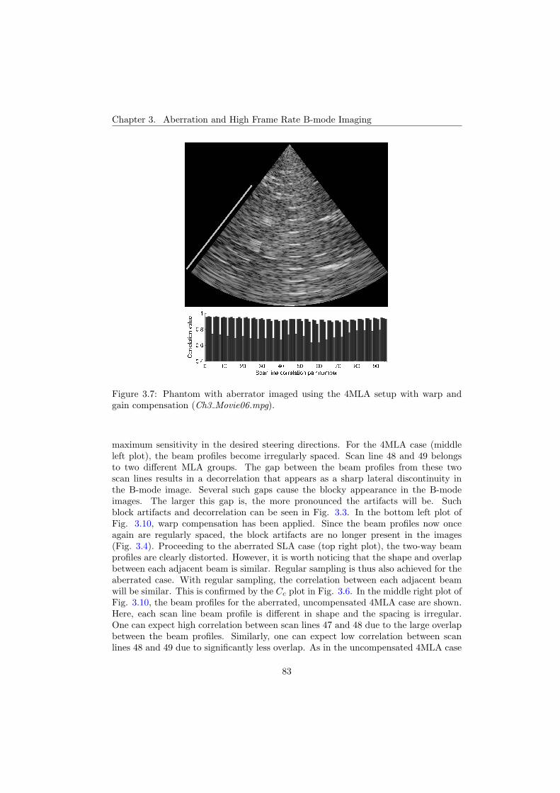
Chapter 3. Aberration and High Frame Rate B-mode Imaging
Figure 3.7: Phantom with aberrator imaged using the 4MLA setup with warp andgain compensation (Ch3 Movie06.mpg).
maximum sensitivity in the desired steering directions. For the 4MLA case (middleleft plot), the beam profiles become irregularly spaced. Scan line 48 and 49 belongsto two different MLA groups. The gap between the beam profiles from these twoscan lines results in a decorrelation that appears as a sharp lateral discontinuity inthe B-mode image. Several such gaps cause the blocky appearance in the B-modeimages. The larger this gap is, the more pronounced the artifacts will be. Suchblock artifacts and decorrelation can be seen in Fig. 3.3. In the bottom left plot ofFig. 3.10, warp compensation has been applied. Since the beam profiles now onceagain are regularly spaced, the block artifacts are no longer present in the images(Fig. 3.4). Proceeding to the aberrated SLA case (top right plot), the two-way beamprofiles are clearly distorted. However, it is worth noticing that the shape and overlapbetween each adjacent beam is similar. Regular sampling is thus also achieved for theaberrated case. With regular sampling, the correlation between each adjacent beamwill be similar. This is confirmed by the Cc plot in Fig. 3.6. In the middle right plot ofFig. 3.10, the beam profiles for the aberrated, uncompensated 4MLA case are shown.Here, each scan line beam profile is different in shape and the spacing is irregular.One can expect high correlation between scan lines 47 and 48 due to the large overlapbetween the beam profiles. Similarly, one can expect low correlation between scanlines 48 and 49 due to significantly less overlap. As in the uncompensated 4MLA case
83
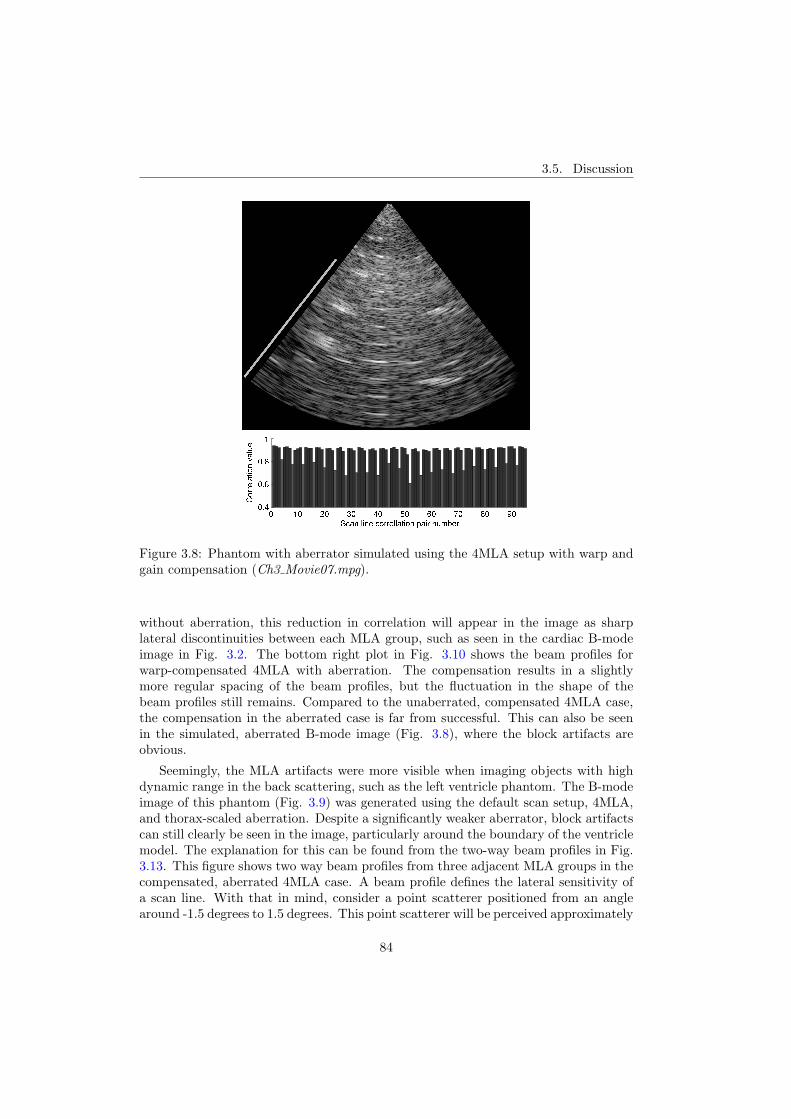
3.5. Discussion
Figure 3.8: Phantom with aberrator simulated using the 4MLA setup with warp andgain compensation (Ch3 Movie07.mpg).
without aberration, this reduction in correlation will appear in the image as sharplateral discontinuities between each MLA group, such as seen in the cardiac B-modeimage in Fig. 3.2. The bottom right plot in Fig. 3.10 shows the beam profiles forwarp-compensated 4MLA with aberration. The compensation results in a slightlymore regular spacing of the beam profiles, but the fluctuation in the shape of thebeam profiles still remains. Compared to the unaberrated, compensated 4MLA case,the compensation in the aberrated case is far from successful. This can also be seenin the simulated, aberrated B-mode image (Fig. 3.8), where the block artifacts areobvious.
Seemingly, the MLA artifacts were more visible when imaging objects with highdynamic range in the back scattering, such as the left ventricle phantom. The B-modeimage of this phantom (Fig. 3.9) was generated using the default scan setup, 4MLA,and thorax-scaled aberration. Despite a significantly weaker aberrator, block artifactscan still clearly be seen in the image, particularly around the boundary of the ventriclemodel. The explanation for this can be found from the two-way beam profiles in Fig.3.13. This figure shows two way beam profiles from three adjacent MLA groups in thecompensated, aberrated 4MLA case. A beam profile defines the lateral sensitivity ofa scan line. With that in mind, consider a point scatterer positioned from an anglearound -1.5 degrees to 1.5 degrees. This point scatterer will be perceived approximately
84
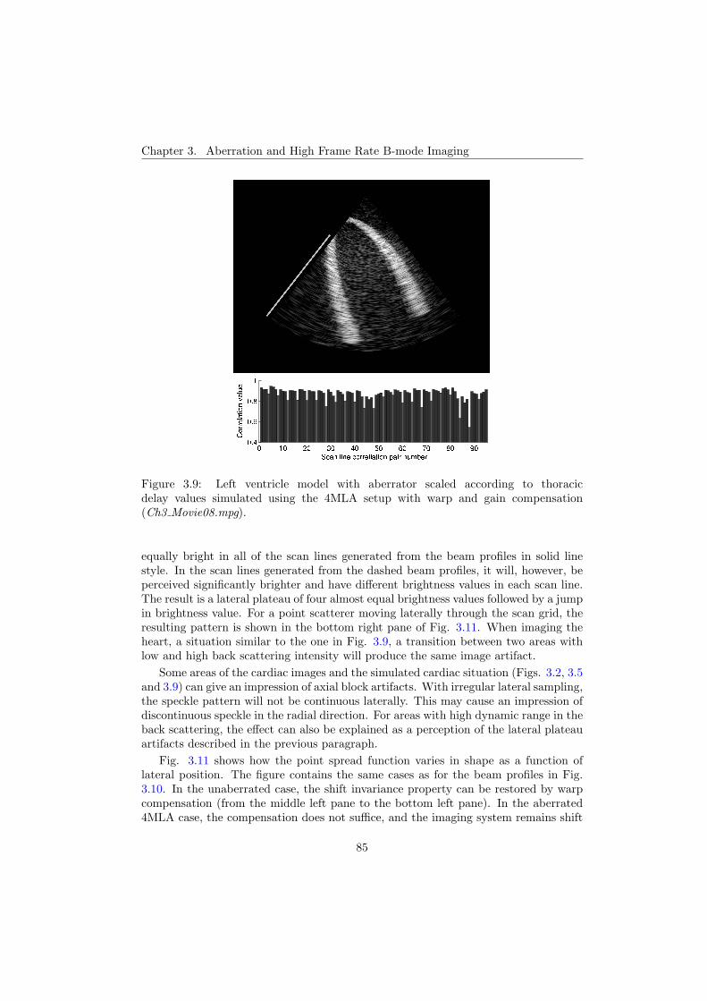
Chapter 3. Aberration and High Frame Rate B-mode Imaging
Figure 3.9: Left ventricle model with aberrator scaled according to thoracicdelay values simulated using the 4MLA setup with warp and gain compensation(Ch3 Movie08.mpg).
equally bright in all of the scan lines generated from the beam profiles in solid linestyle. In the scan lines generated from the dashed beam profiles, it will, however, beperceived significantly brighter and have different brightness values in each scan line.The result is a lateral plateau of four almost equal brightness values followed by a jumpin brightness value. For a point scatterer moving laterally through the scan grid, theresulting pattern is shown in the bottom right pane of Fig. 3.11. When imaging theheart, a situation similar to the one in Fig. 3.9, a transition between two areas withlow and high back scattering intensity will produce the same image artifact.
Some areas of the cardiac images and the simulated cardiac situation (Figs. 3.2, 3.5and 3.9) can give an impression of axial block artifacts. With irregular lateral sampling,the speckle pattern will not be continuous laterally. This may cause an impression ofdiscontinuous speckle in the radial direction. For areas with high dynamic range in theback scattering, the effect can also be explained as a perception of the lateral plateauartifacts described in the previous paragraph.
Fig. 3.11 shows how the point spread function varies in shape as a function oflateral position. The figure contains the same cases as for the beam profiles in Fig.3.10. In the unaberrated case, the shift invariance property can be restored by warpcompensation (from the middle left pane to the bottom left pane). In the aberrated4MLA case, the compensation does not suffice, and the imaging system remains shift
85

3.5. Discussion
Figure 3.10: Simulated two-way beam profiles from four adjacent scan lines. Theapplied setup is given in Table 4.1. The vertical lines indicate the desired steeringdirection of the beam profiles in corresponding line style. Ideally these lines shouldintersect their beam profiles at their maximum. Left side: Without aberration.Right side: With aberration. Top: SLA. Middle: Uncompensated 4MLA. Bottom:Compensated 4MLA. In the 4MLA cases, the beam profiles in solid and dashed linestyle are the two last beams in a 4MLA group. The beam profiles in dash-dotted anddotted line style are the first two beams from the adjacent 4MLA group. Notice thatwith the combination of 4MLA and aberration, each scan line beam profile is differentin shape, has different gain, and has irregular spacing.
variant (middle right pane and bottom right pane). This confirms the measured results.Both the measured and simulated results showed that repeating patterns in the
Cc plots were related to the presence of block artifacts in the corresponding B-modeimages. The Dc values shown in Table 3.2 quantify the magnitude of these patternsand confirm the impression from images and Cc plots. The situation with 4MLAwithout aberration (Fig. 3.4) produced a negative Dc value. This indicates that thecorrelation at transitions between MLA groups was stronger than within the MLAgroups. The reason for this might be overcompensation for the warping effect.
Larger Dc values were measured with the aberrated phantom images than in thecardiac images. This was probably because the RMS delay values of the siliconaberrator were from abdominal measurements. To investigate a cardiac imagingsituation, the aberrator was scaled to thoracic RMS delay values in simulations andused to image the left ventricle computer phantom. The resulting image and Cc
86
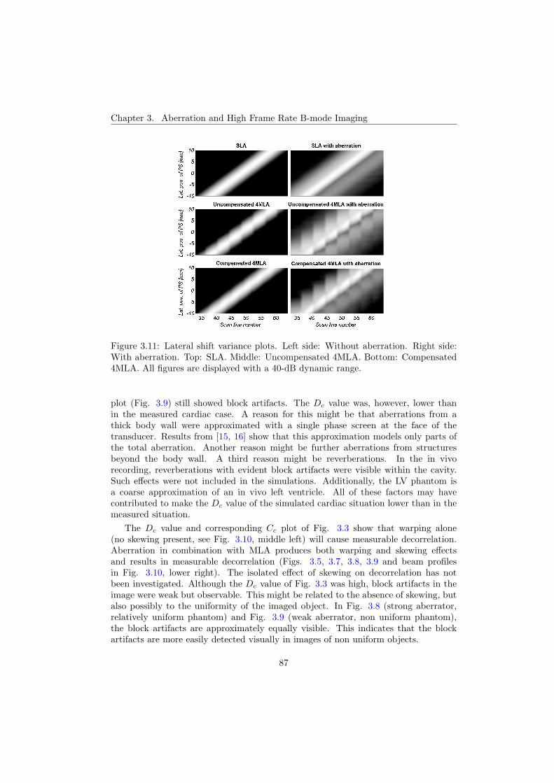
Chapter 3. Aberration and High Frame Rate B-mode Imaging
Figure 3.11: Lateral shift variance plots. Left side: Without aberration. Right side:With aberration. Top: SLA. Middle: Uncompensated 4MLA. Bottom: Compensated4MLA. All figures are displayed with a 40-dB dynamic range.
plot (Fig. 3.9) still showed block artifacts. The Dc value was, however, lower thanin the measured cardiac case. A reason for this might be that aberrations from athick body wall were approximated with a single phase screen at the face of thetransducer. Results from [15, 16] show that this approximation models only parts ofthe total aberration. Another reason might be further aberrations from structuresbeyond the body wall. A third reason might be reverberations. In the in vivorecording, reverberations with evident block artifacts were visible within the cavity.Such effects were not included in the simulations. Additionally, the LV phantom isa coarse approximation of an in vivo left ventricle. All of these factors may havecontributed to make the Dc value of the simulated cardiac situation lower than in themeasured situation.
The Dc value and corresponding Cc plot of Fig. 3.3 show that warping alone(no skewing present, see Fig. 3.10, middle left) will cause measurable decorrelation.Aberration in combination with MLA produces both warping and skewing effectsand results in measurable decorrelation (Figs. 3.5, 3.7, 3.8, 3.9 and beam profilesin Fig. 3.10, lower right). The isolated effect of skewing on decorrelation has notbeen investigated. Although the Dc value of Fig. 3.3 was high, block artifacts in theimage were weak but observable. This might be related to the absence of skewing, butalso possibly to the uniformity of the imaged object. In Fig. 3.8 (strong aberrator,relatively uniform phantom) and Fig. 3.9 (weak aberrator, non uniform phantom),the block artifacts are approximately equally visible. This indicates that the blockartifacts are more easily detected visually in images of non uniform objects.
87

3.6. Conclusions
Figure 3.12: Illustration of how LSV plots are generated. Top: Image of a pointscatterer at a lateral position at focus depth. Middle: Radial mean square value of thepoint scatterer image. Bottom: Stacked radial mean square values for several pointscatterer positions. The dashed line indicates the position of the radial mean squarevalue in the middle pane.
Figure 3.13: Two-way beam profiles from three adjacent 4MLA groups. The simulationsetup was 4MLA with aberration and warp compensation. Group 11 plotted in solid,group 12 in dashed and group 13 in dotted line style.
3.6 Conclusions
Simulations and in vitro experiments showed that aberration in combination withparallel beamforming caused block artifacts similar to the artifacts observed in cardiacparallel beamforming images. Gain and beam steering compensation successful in non-aberrated in vitro cases failed in aberrated in vitro cases.
During investigation of simulated beam profiles, two underlying mechanisms were
88

Chapter 3. Aberration and High Frame Rate B-mode Imaging
identified. The first mechanism was irregular sampling and decorrelation. This wascaused by aberration distorting and pulling the beam profiles out of the original scangrid, leaving gaps between the parallel receive groups. Second, the asymmetric andvariable shape of the beam profiles caused a stair-like gain variation in transitionsbetween imaged areas with low and high intensity.
Acknowledgement
The authors thank GE Vingmed Ultrasound for access to the Vivid 7 ultrasoundscanner.
89

3.6. Conclusions
90

References
[1] D. P. Shattuck, M. D. Weinshenker, S. W. Smith, and O. T. von Ramm,“Explososcan: A parallel processing technique for high speed ultrasound imagingwith linear phased arrays,” J Acoust Soc Amer, vol. 75, no. 4, pp. 1273–1282,1984.
[2] O. T. von Ramm, S. W. Smith, and H. G. Pavy, “High-speed ultrasoundvolumetric imaging system – part II: Parallel processing and image display,” IEEETrans Ultrason Ferroelectr Freq Control, vol. 38, pp. 109–115, March 1991.
[3] G. L. Holley and I. M. Guracar, “Ultrasound multi-beam distortion correctionsystem and method.” U.S. Patent 5.779.640, July 14 1998.
[4] J. N. Wright, S. H. Maslak, D. J. Finger, and A. Gee, “Method and apparatusfor coherent image formation.” U.S. Patent 5.623.928, Apr. 29 1997.
[5] T. Hergum, T. Bjastad, and H. Torp, “Parallel beamforming using synthetictransmit beams,” Proc IEEE Ultrason Symp, vol. 2, pp. 1401–4, 2004.
[6] D.-L. D. Liu, J. C. Lazenby, Z. Banjanin, and B. A. McDermot, “System andmethod for reduction of parallel beamforming artifacts.” U.S. Patent 6.447.452,Sep. 10 2002.
[7] T. J. Hunt, B. M. Herrick, K. K. Robertson, and J. M. Ziel, “Ultrasonic imagingsystem using line splicing and parallel receive beam formation.” U.S. patent5.462.057, Oct. 31 1995.
[8] S. M. Kay, Fundamentals of Statistical Signal Processing: Estimation Theory.Indianapolis, IN: Prentice-Hall PTR, 1993.
[9] H. L. V. Trees, Detection, Estimation and Modulation Theory, Part I: Detection,Estimation, and Linear Modulation Theory. New York: Wiley, 2001.
[10] T. F. Johansen, B. A. J. Angelsen, and W. Nordhøy, “Phase aberrations -Experiments and simulations,” Proc 23rd Scand Symp Phys Acoust, pp. 57–60,2000.
91
References
[11] L. M. Hinkelman, D.-L. Liu, L. A. Metlay, and R. C. Waag, “Measurements ofultrasonic pulse arrival time and energy level variations produced by propagationthrough abdominal wall,” J Acoust Soc Am, vol. 95, no. 1, pp. 530–541, 1994.
[12] L. M. Hinkelman, T. L. Szabo, and R. C. Waag, “Measurements of ultrasonicpulse distortion produced by human chest wall,” J Acoust Soc Am, vol. 101,no. 4, pp. 2365–2373, 1997.
[13] J. A. Jensen and N. B. Svendsen, “Calculation of pressure fields from arbitrarilyshaped, apodized, and excited ultrasound transducers,” IEEE Trans UltrasonFerroelectr Freq Control, vol. 39, pp. 262–267, 1992.
[14] S. Rabben, A. Haukanes, and F. Irgens, “A kinematic model for simulatingphysiological left ventricular deformation patterns - a tool for evaluation ofmyocardial strain imaging,” Proc IEEE Ultrason Symp, pp. 134–7, 2003.
[15] L. M. Hinkelman, T. D. Mast, L. A. Metlay, and R. C. Waag, “The effect ofabdominal wall morphology on ultrasonic pulse distortion. part i. measurements,”J Acoust Soc Am, vol. 104, no. 6, pp. 3635–3649, 1998.
[16] T. D. Mast, L. M. Hinkelman, M. J. Orr, V. W. Sparrow, and R. C. Waag,“Simulation of ultrasonic pulse propagation through the abdominal wall,” JAcoust Soc Am, vol. 102, no. 2, pp. 1177–1190, 1997.
92
Chapter 4
Synthetic Transmit BeamTechnique in an AberratingEnvironmentT. Bjastad and H. TorpDept. Circulation and Medical Imaging, NTNU
Parallel beamforming is a common method for increasing the frame ratein ultrasound imaging systems. By receiving in several directions for eachtransmit event, the frame rate is increased. However, this method alsointroduces block-like artifacts in the B-mode image due to the receive offsetscompared to the transmit direction. The synthetic transmit beam technique,STB, has previously been proposed as a compensation technique to addressthese artifacts by creating synthetic transmit beams in each of the receivedirections. Previous work by Hergum et al. investigated the performance ofthis method in the case of two parallel beams in tissue mimicking phantomswithout aberrations.This study is a continuation of that work, where the method is tested inan aberrating environment using four parallel beams. Several quantitativeand qualitative performance aspects of the method has been investigated:Lateral shift invariance, beam to beam correlation fluctuations, speckletracking performance, improvements from higher order STB interpolation,beam profile shape preservation as well as perceived image qualityimprovements. The results were obtained from simulations, in vivo and invitro measurements.The results showed that aberration amplified the image artifacts for regularparallel beamforming, resulting in more shift variance, lower beam tobeam correlation, higher speckle tracking error and more variation in beamprofile shape. Compared to regular parallel beamforming, STB resulted insignificantly better image quality and a higher score in all measuring methods.The improvements from using STB were largest in the cases with aberration.Here, the variation in beam to beam correlation was reduced from 30% to 1%using STB.
93
4.1. Introduction
4.1 Introduction
Increased frame rate is desirable in a number of ultrasound applications, particularlyin cardiac three-dimensional imaging, but also in several two-dimensional applications.One example is duplex and triplex imaging, where several imaging modes are runningsimultaneously, such as B-mode, color flow and PW-Doppler. Compounding will alsobenefit from increased acquisition speed, as will multi-plane B-mode imaging, whereseveral 2D B-mode scan planes are acquired simultaneously using a 2D array. Highframe rates are also required for accurate tracking of cardiac tissue [1].
A common technique for increasing the frame rate is parallel beamforming [2, 3].Using this technique, several scan lines are acquired in parallel from each transmitevent. Parallel beamforming is therefore also known as multi-line acquisition (MLA).This technique increases the frame rate proportional to the number of parallel receivebeams, but, as shown in [4, 5], the method also introduces artifacts in the images,typically giving them a blocky appearance. Such artifacts will be referred to as MLAartifacts.
The source of these artifacts is the inherent misalignment of the transmit andreceive beams. The interaction between the transmit and receive beams when theyare not pointing in the same direction causes distortions of the two-way beam profiles.These distortions can be split into two components: Warping and skewing. Thewarping effect causes the maximum point of the two-way beam profile to be shiftedtowards the transmit beam direction (in other words, the two-way beam direction isnot the same as the receive beam direction). This results in a non-uniform lateralsampling of the imaged object. The skewing effect causes the two-way beam profilesto be asymmetrical. In addition, sensitivity is decreased as the receive beams aresteered away from the transmit beam main lobe direction, resulting in gain variations[4, 5]. Since the warping, skewing and gain variation are related to beam geometry,they will be depth dependent. The severity of the effects will depend on how much thereceive direction is offset compared to the transmit direction; hence the two-way beamprofile shape will be different from scan line to scan line. The severity also depends onthe width of the transmit beams relative to the receive beams. Reducing the transmitaperture will increase the beam width and thus reduce the warping and skewing [6].However, it will also reduce penetration and resolution.
It is likely that the MLA artifacts will decrease the performance of speckle tracking.As shown in [5], parallel beamforming imaging systems will be shift variant, i.e. theimage of a point scatterer will be dependent on its position. Speckle tracking methodsassume that the speckle pattern is preserved during tissue movement. Shift variancewill most likely reduce the validity of this assumption.
Several techniques have been proposed to compensate for MLA artifacts. In [7], atransmit sinc apodization was proposed to obtain a transmit beam with a rectangularshape. This would reduce the warping effect, but the skewing effect would still bepresent. Also, both resolution and penetration would be reduced due to the reducedeffective transmit aperture.
In US Patents 5779640 [8] and 6447452 [9], the authors describe incoherent methodsfor beam interpolation applied after detection of the RF signal. These methods
94
Chapter 4. Synthetic Transmit Beam Technique in an Aberrating Environment
compensate for warping by interpolating from a non-uniform scan grid to a regularscan grid before display. These methods do not compensate for skewing.
Another compensation technique is presented in US Patent 5462057 [10]. In thispatent, the authors propose dynamic steering of the receive beams to counteract thewarping effect throughout the imaging depth. However, this does require predictionor estimation of the warping at all depths. It will also increase skewing due to theincreased receive offset.
The technique that has been investigated in this study is the synthetic transmitbeam technique, STB. This technique reduces the effect of both skewing and warpingand has previously been described in [5] and US Patent 5318033 [11]. The basicprinciple is to create synthetic transmit beams in all parallel receive directions. Ideally,this eliminates the effect of the transmit-receive offset in parallel beamforming. In [5],Hergum et al. showed that this technique strongly reduced MLA artifacts for twoparallel beams in tissue mimicking phantoms without aberrations.
Due to inhomogeneities in the body wall, transthoracic imaging will always beaffected by some degree of aberration. This aberration can result in distortions andasymmetry in the beam profiles.
Previous work presented in [4] applied a steering compensation method to reduceMLA artifacts. This method was similar to the dynamic steering method presentedin [10], and counteracted the warping effect by adding offsets to the receive beamdirections. The technique was shown to strongly reduce MLA artifacts in unaberratedphantom recordings. However, when using the same correction values in aberratedphantom recordings, the image artifacts remained. The presence of aberrationdistorted the beam profiles and invalidated the pre-programmed correction offsets.Since inhomogeneities causing aberrations are unknown, valid correction offsets aredifficult to estimate. Similarly, this will also be a weakness in the beam interpolationmethods presented in [8] and [9]. To some degree, the sinc apodization methodpresented in [7] will also be affected by aberration, since it relies on a certain transmitbeam shape. STB, on the other hand, is a blind correction technique, requiringnothing more than a certain acquisition pattern. Given a thin aberrator close tothe transducer surface, adequate beam density and ideal interpolation, STB shouldtheoretically perform identically to single line acquisition.
In this work we investigate how well the STB technique performs in a realistic,aberrating environment using four parallel beams and linear STB interpolation. Theperformance is evaluated using several quantitative and qualitative measures.
Section II contains the theory behind STB and the methods used for analysis.Section III presents the simulation and measurement setup. Section IV contains theresults. These results are discussed in Section V, with conclusions presented in SectionVI.
4.2 Theory
The number of parallel beams will be indicated by the number in front of the MLAand STB abbreviations. For instance, 4MLA indicates four parallel beams and 4STB
95
4.2. Theory
indicates four output STB beams. The group of receive beams belonging to onetransmit event will be termed parallel receive group or MLA group. Normal acquisitionwith one receive beam per transmit beam will be termed single line acquisition, SLA.
4.2.1 Two-way response and the point spread function
In this work, we define the two way response according to the pulse-echo formulationin [12]:
v0 = eT �t gT �t ht �t hr �t gR, (4.1)
where �t is a temporal convolution operator, eT is the excitation pulse, gT and gR
are the transducer impulse responses on transmit and receive, ht is the spatial impulseresponse on transmit and hr is the spatial impulse response on receive.
The point spread function is defined as the image obtained from imaging a singlepoint scatterer. For SLA imaging, the PSF will be identical to the two-way response,assuming that the two-way response is constant for all imaging beams. However, usingparallel beamforming, the two-way response becomes variant from beam to beam.Hence the PSF will be the image obtained from sampling a point scatterer in a gridof beams with different two-way responses.
4.2.2 The Synthetic Transmit Beam method
As explained in the introduction, the source of MLA artifacts is the misalignment of thetransmit and receive beams. The basic idea of STB is therefore to create a synthetictransmit beam for each receive beam direction. This is done through interpolationon channel data between neighboring transmit events. Since a single element is smallcompared to the wavelength, it can be considered omni directional. The resolution ofan image obtained from receiving on a single element will then be determined almostsolely by the transmit beam width. Hence, the lateral spatial bandwidth of imagefrom a single element is determined by the transmit aperture. So as long as thetransmit beam spacing satisfies the Nyquist sampling theorem for this bandwidth,data from any intervening transmit beam can be reconstructed using interpolation.Given adequate transmit beam density and ideal interpolation, each receive beam canthen be perfectly aligned with a synthetic or real transmit beam as if traditional SLAhad been used [5, 11].
4.2.3 STB and aberrations
Aberrations occurring close to the transducer surface can be modeled as simplealternations of the aperture function (phase and amplitude). This will result in higherside lobes and other distortions to the transmitted ultrasound pulse. It will howevernot change the lateral spatial bandwidth of the pulse. Hence, the requirements of theSTB method to reconstruct intervening transmit beams is not violated. While theartifacts of regular MLA is amplified by aberrations [4], one can therefore assume thatSTB will perform just as well both with and without aberrations.
96
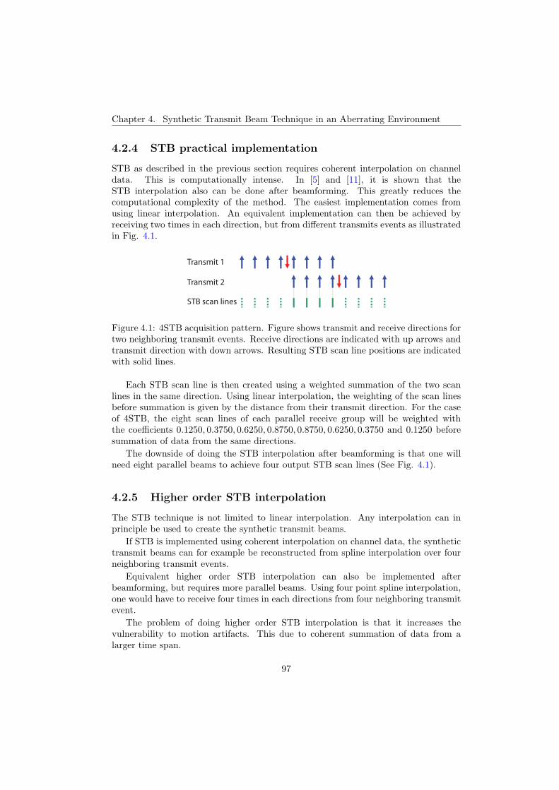
Chapter 4. Synthetic Transmit Beam Technique in an Aberrating Environment
4.2.4 STB practical implementation
STB as described in the previous section requires coherent interpolation on channeldata. This is computationally intense. In [5] and [11], it is shown that theSTB interpolation also can be done after beamforming. This greatly reduces thecomputational complexity of the method. The easiest implementation comes fromusing linear interpolation. An equivalent implementation can then be achieved byreceiving two times in each direction, but from different transmits events as illustratedin Fig. 4.1.
Transmit 1
Transmit 2
STB scan lines
Figure 4.1: 4STB acquisition pattern. Figure shows transmit and receive directions fortwo neighboring transmit events. Receive directions are indicated with up arrows andtransmit direction with down arrows. Resulting STB scan line positions are indicatedwith solid lines.
Each STB scan line is then created using a weighted summation of the two scanlines in the same direction. Using linear interpolation, the weighting of the scan linesbefore summation is given by the distance from their transmit direction. For the caseof 4STB, the eight scan lines of each parallel receive group will be weighted withthe coefficients 0.1250, 0.3750, 0.6250, 0.8750, 0.8750, 0.6250, 0.3750 and 0.1250 beforesummation of data from the same directions.
The downside of doing the STB interpolation after beamforming is that one willneed eight parallel beams to achieve four output STB scan lines (See Fig. 4.1).
4.2.5 Higher order STB interpolation
The STB technique is not limited to linear interpolation. Any interpolation can inprinciple be used to create the synthetic transmit beams.
If STB is implemented using coherent interpolation on channel data, the synthetictransmit beams can for example be reconstructed from spline interpolation over fourneighboring transmit events.
Equivalent higher order STB interpolation can also be implemented afterbeamforming, but requires more parallel beams. Using four point spline interpolation,one would have to receive four times in each directions from four neighboring transmitevent.
The problem of doing higher order STB interpolation is that it increases thevulnerability to motion artifacts. This due to coherent summation of data from alarger time span.
97
4.2. Theory
4.2.6 Metrics to measure parallel beamforming artifact
Much of the literature on parallel beamforming compensation methods is to be foundin patents. Due to this, there are few established methods on how to evaluate andquantify the artifacts.
First of all, the B-mode artifacts are mostly a visual disturbance. It does notdecrease contrast resolution or spatial resolution and the human eye can in most caseseasily determine that the artifacts are not physical features of the imaged object. Butthey remove attention from the actual imaged object, and any ultrasound clinicianwould like them removed.
The artifacts appear as a stationary blocky pattern in the image. What thisactually shows, is that the imaging system is spatially shift variant. Ideally, the imageof an object should be the same regardless of its position relative to the probe. Butfor a shift variant imaging system, the object image will change with object position.
For an imaging system to be shift invariant there are some factors that must be inplace:
1. The two-way response of each imaging beam must be equal in shape.
2. The two-way response of each imaging beam must be equally spaced.
3. The distance between each imaging beam must satisfy the Nyquist samplingtheorem.
The problem of parallel beamforming lies mainly in item 1 and 2. Skewing andwarping results in varying shape and spacing of the two way responses. Item 3 assumesideal lateral interpolation to avoid aliasing errors after detection. If not, the imagingsystem will still be spatially shift variant, even if 1 and 2 is satisfied. Since idealinterpolation can not be achieved in practical situations, the beam density should besomewhat higher than the Nyquist sampling limit to reduce aliasing errors. Typicallysome degree of under sampling and aliasing errors are tolerated when high frame rateis a priority.
Using simulations and measurements, the metrics used in this work tries toinvestigate and measure to what extend the three above listed requirements aresatisfied using parallel beamforming with and without synthetic transmit beams.
Lateral Shift Variance (LSV) plots
LSV (Lateral Shift Variance) plots, such as those in Fig. 4.7 can be used to investigatethe spatial invariance of an imaging system [4, 5]. They are created by simulatingimages of a point scatterer moving through the imaging sector. Each image will thencorrespond to the PSF of the system at the point scatterer location. For a shiftinvariant system, the resulting PSFs should be constant in shape. Since visualizingthe whole 2D PSF in different positions is not suitable in printed form, the LSV plotsshow the axial mean square values of the PSFs instead. Each row in the LSV image
98

Chapter 4. Synthetic Transmit Beam Technique in an Aberrating Environment
Figure 4.2: Illustration of how LSV plots are generated. Top: Image of a pointscatterer at a lateral position at focus depth. Middle: Radial mean square value of thepoint scatterer image. Bottom: Stacked radial mean square values for several pointscatterer positions. The dashed line indicates the position of the radial mean squarevalue in the middle pane. Top and bottom images are shown with a dynamic range of40 dB.
corresponds to a PSF at the position indicated by the y-axis. This provides a plotwhere it is easy to evaluate the spatial variance of the system. If the system is shiftinvariant, the LSV plot should show a straight diagonal structure. Deviations froma straight diagonal structure, such as in Fig. 4.2, indicate that the PSF varies withlateral position and that the system is shift variant. LSV plots also visualize theresulting MLA artifacts through the whole dynamic range of the B-mode image.
Correlation Analysis
Assuming Rayleigh scattering conditions, the authors in [13] show that theautocorrelation for a complex amplitude process equals the scaled autocorrelationof the two way response. This allow us to predict the correlation between scan linesfrom their corresponding two-way responses. In vivo, with aberrations, the two-wayresponses are unknown, but from the same relation we can get information about thetwo-way responses by estimating the scan line correlation from recordings.
In normal single line acquisition, the two-way responses are equally spaced andconstant from beam to beam, resulting in a consistent cross correlation betweenneighboring scan lines. Due to warping and skewing, parallel beamforming two wayresponses are variant from beam to beam. This results in a variation in beam to beamcorrelation.
The work presented in [4] used variation in beam to beam correlation as aquantitative measure of the amount of MLA artifacts in recorded B-mode images.Pairs of neighboring beams across MLA groups were showed to have consistently lowercorrelation than pairs within MLA groups. This is caused by the transmit beams whichpull the two way responses in opposite directions at these location. The location of
99

4.2. Theory
the correlation drops corresponded to the lateral discontinuities in the images and themagnitude of the drops seemed to correspond to the visibility of the artifacts in theimages. When estimating the cross correlation from measurements there will alwaysbe a variance in the estimates. This could obscure the drop in correlation betweenMLA-groups. The cross correlation estimator that would differentiate best is in [4]showed to be as follows:
Cc =2Real(Rij)Rii + Rjj
, (4.2)
where the Rij estimate is calculated as correlation between IQ data in scan linesi and j averaged over a depth range. Cc values for all neighboring scan lines can beplotted to visualize the correlation variation across the image. An overall percentagecorrelation variation can be calculated as follows [4]:
Cd =1N
∑ij∈W Cc − 1
M
∑ij∈T Cc
1N
∑ij∈W Cc
· 100, (4.3)
where ij is a pair of adjacent scan lines. The set W contains all such pairs withinMLA groups, and the set T contains all such pairs located at transitions betweenMLA groups. N is the size of the set W , and M is the size of the set T . A good Cd
value should be as close as possible to zero since this indicates an even beam to beamcorrelation throughout the image. Using regular MLA, the value will in general bepositive since the correlation within the MLA groups is larger than at the transitionsbetween MLA groups.
If the two-way responses are known, the Cc values can be calculated by insertingthe cross correlation of the two-way responses for Rij in Eq. 4.2.
Speckle Tracking
Speckle tracking is a technique for evaluating cardiac tissue deformation. The reflectedultrasound from a tissue region creates a distinct interference pattern, called speckle,which can be followed from frame to frame to determine local tissue movement. 2Dspeckle tracking can only track points inside the imaging plane. Object movement outof the imaging plane will result in decorrelation and degraded tracking performance.Due to high tissue velocities and object movement in and out of the imaging plane, ahigh frame rate is desirable when performing 2D cardiac speckle tracking [1, 14]. Thiscan be achieved by using parallel beamforming. However, uncompensated parallelbeamforming results in a shift variant imaging system [4, 5]. Shift variance will causethe speckle pattern to change with object position, and is therefore likely to influencethe speckle tracking accuracy. This makes speckle tracking suitable as a metric forcomparing SLA, MLA and STB.
According to theory, ideal STB should perform just as well with speckle trackingas SLA. Since aberration not should impact STB shift variance, one can also predict
100
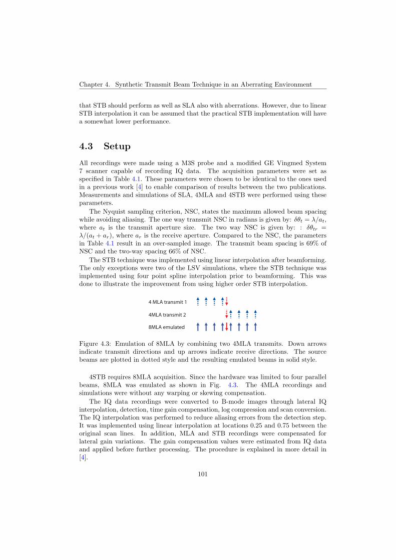
Chapter 4. Synthetic Transmit Beam Technique in an Aberrating Environment
that STB should perform as well as SLA also with aberrations. However, due to linearSTB interpolation it can be assumed that the practical STB implementation will havea somewhat lower performance.
4.3 Setup
All recordings were made using a M3S probe and a modified GE Vingmed System7 scanner capable of recording IQ data. The acquisition parameters were set asspecified in Table 4.1. These parameters were chosen to be identical to the ones usedin a previous work [4] to enable comparison of results between the two publications.Measurements and simulations of SLA, 4MLA and 4STB were performed using theseparameters.
The Nyquist sampling criterion, NSC, states the maximum allowed beam spacingwhile avoiding aliasing. The one way transmit NSC in radians is given by: δθt = λ/at,where at is the transmit aperture size. The two way NSC is given by: : δθtr =λ/(at + ar), where ar is the receive aperture. Compared to the NSC, the parametersin Table 4.1 result in an over-sampled image. The transmit beam spacing is 69% ofNSC and the two-way spacing 66% of NSC.
The STB technique was implemented using linear interpolation after beamforming.The only exceptions were two of the LSV simulations, where the STB technique wasimplemented using four point spline interpolation prior to beamforming. This wasdone to illustrate the improvement from using higher order STB interpolation.
4 MLA transmit 1
4MLA transmit 2
8MLA emulated
Figure 4.3: Emulation of 8MLA by combining two 4MLA transmits. Down arrowsindicate transmit directions and up arrows indicate receive directions. The sourcebeams are plotted in dotted style and the resulting emulated beams in solid style.
4STB requires 8MLA acquisition. Since the hardware was limited to four parallelbeams, 8MLA was emulated as shown in Fig. 4.3. The 4MLA recordings andsimulations were without any warping or skewing compensation.
The IQ data recordings were converted to B-mode images through lateral IQinterpolation, detection, time gain compensation, log compression and scan conversion.The IQ interpolation was performed to reduce aliasing errors from the detection step.It was implemented using linear interpolation at locations 0.25 and 0.75 between theoriginal scan lines. In addition, MLA and STB recordings were compensated forlateral gain variations. The gain compensation values were estimated from IQ dataand applied before further processing. The procedure is explained in more detail in[4].
101
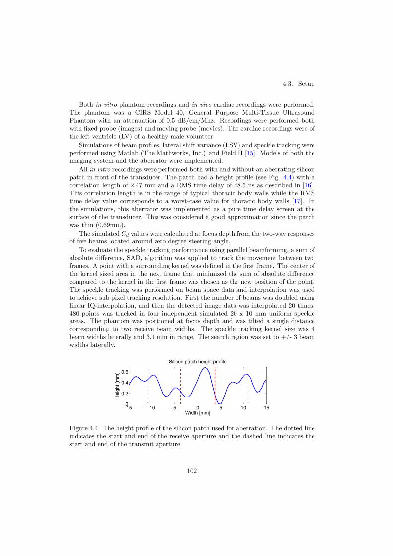
4.3. Setup
Both in vitro phantom recordings and in vivo cardiac recordings were performed.The phantom was a CIRS Model 40, General Purpose Multi-Tissue UltrasoundPhantom with an attenuation of 0.5 dB/cm/Mhz. Recordings were performed bothwith fixed probe (images) and moving probe (movies). The cardiac recordings were ofthe left ventricle (LV) of a healthy male volunteer.
Simulations of beam profiles, lateral shift variance (LSV) and speckle tracking wereperformed using Matlab (The Mathworks, Inc.) and Field II [15]. Models of both theimaging system and the aberrator were implemented.
All in vitro recordings were performed both with and without an aberrating siliconpatch in front of the transducer. The patch had a height profile (see Fig. 4.4) with acorrelation length of 2.47 mm and a RMS time delay of 48.5 ns as described in [16].This correlation length is in the range of typical thoracic body walls while the RMStime delay value corresponds to a worst-case value for thoracic body walls [17]. Inthe simulations, this aberrator was implemented as a pure time delay screen at thesurface of the transducer. This was considered a good approximation since the patchwas thin (0.69mm).
The simulated Cd values were calculated at focus depth from the two-way responsesof five beams located around zero degree steering angle.
To evaluate the speckle tracking performance using parallel beamforming, a sum ofabsolute difference, SAD, algorithm was applied to track the movement between twoframes. A point with a surrounding kernel was defined in the first frame. The center ofthe kernel sized area in the next frame that minimized the sum of absolute differencecompared to the kernel in the first frame was chosen as the new position of the point.The speckle tracking was performed on beam space data and interpolation was usedto achieve sub pixel tracking resolution. First the number of beams was doubled usinglinear IQ-interpolation, and then the detected image data was interpolated 20 times.480 points was tracked in four independent simulated 20 x 10 mm uniform speckleareas. The phantom was positioned at focus depth and was tilted a single distancecorresponding to two receive beam widths. The speckle tracking kernel size was 4beam widths laterally and 3.1 mm in range. The search region was set to +/- 3 beamwidths laterally.
−15 −10 −5 0 5 10 150
0.2
0.4
0.6
Width [mm]
Hei
ght [
mm
]
Silicon patch height profile
Figure 4.4: The height profile of the silicon patch used for aberration. The dotted lineindicates the start and end of the receive aperture and the dashed line indicates thestart and end of the transmit aperture.
102
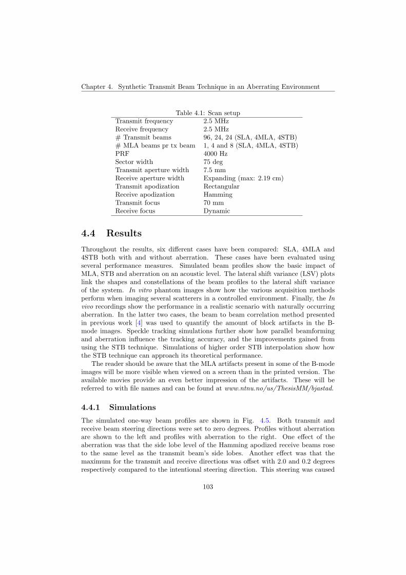
Chapter 4. Synthetic Transmit Beam Technique in an Aberrating Environment
Table 4.1: Scan setupTransmit frequency 2.5 MHzReceive frequency 2.5 MHz# Transmit beams 96, 24, 24 (SLA, 4MLA, 4STB)# MLA beams pr tx beam 1, 4 and 8 (SLA, 4MLA, 4STB)PRF 4000 HzSector width 75 degTransmit aperture width 7.5 mmReceive aperture width Expanding (max: 2.19 cm)Transmit apodization RectangularReceive apodization HammingTransmit focus 70 mmReceive focus Dynamic
4.4 Results
Throughout the results, six different cases have been compared: SLA, 4MLA and4STB both with and without aberration. These cases have been evaluated usingseveral performance measures. Simulated beam profiles show the basic impact ofMLA, STB and aberration on an acoustic level. The lateral shift variance (LSV) plotslink the shapes and constellations of the beam profiles to the lateral shift varianceof the system. In vitro phantom images show how the various acquisition methodsperform when imaging several scatterers in a controlled environment. Finally, the Invivo recordings show the performance in a realistic scenario with naturally occurringaberration. In the latter two cases, the beam to beam correlation method presentedin previous work [4] was used to quantify the amount of block artifacts in the B-mode images. Speckle tracking simulations further show how parallel beamformingand aberration influence the tracking accuracy, and the improvements gained fromusing the STB technique. Simulations of higher order STB interpolation show howthe STB technique can approach its theoretical performance.
The reader should be aware that the MLA artifacts present in some of the B-modeimages will be more visible when viewed on a screen than in the printed version. Theavailable movies provide an even better impression of the artifacts. These will bereferred to with file names and can be found at www.ntnu.no/us/ThesisMM/bjastad.
4.4.1 Simulations
The simulated one-way beam profiles are shown in Fig. 4.5. Both transmit andreceive beam steering directions were set to zero degrees. Profiles without aberrationare shown to the left and profiles with aberration to the right. One effect of theaberration was that the side lobe level of the Hamming apodized receive beams roseto the same level as the transmit beam’s side lobes. Another effect was that themaximum for the transmit and receive directions was offset with 2.0 and 0.2 degreesrespectively compared to the intentional steering direction. This steering was caused
103
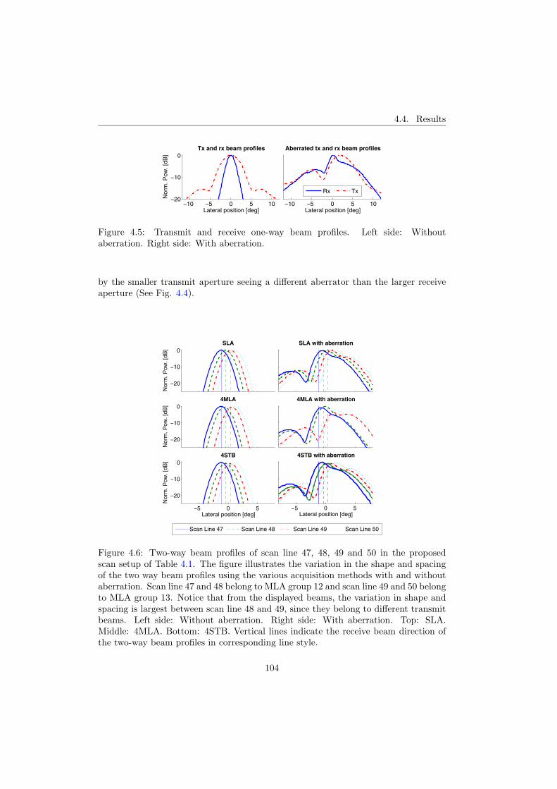
4.4. Results
−10 −5 0 5 10−20
−10
0
Lateral position [deg]
Nor
m. P
ow. [
dB]
Tx and rx beam profiles
−10 −5 0 5 10Lateral position [deg]
Aberrated tx and rx beam profiles
Rx Tx
Figure 4.5: Transmit and receive one-way beam profiles. Left side: Withoutaberration. Right side: With aberration.
by the smaller transmit aperture seeing a different aberrator than the larger receiveaperture (See Fig. 4.4).
−20
−10
0
Nor
m. P
ow. [
dB]
SLA
−20
−10
0
Nor
m. P
ow. [
dB]
4MLA
−5 0 5
−20
−10
0
Lateral position [deg]
Nor
m. P
ow. [
dB]
4STB
SLA with aberration
4MLA with aberration
−5 0 5
4STB with aberration
Lateral position [deg]
Scan Line 47 Scan Line 48 Scan Line 49 Scan Line 50
Figure 4.6: Two-way beam profiles of scan line 47, 48, 49 and 50 in the proposedscan setup of Table 4.1. The figure illustrates the variation in the shape and spacingof the two way beam profiles using the various acquisition methods with and withoutaberration. Scan line 47 and 48 belong to MLA group 12 and scan line 49 and 50 belongto MLA group 13. Notice that from the displayed beams, the variation in shape andspacing is largest between scan line 48 and 49, since they belong to different transmitbeams. Left side: Without aberration. Right side: With aberration. Top: SLA.Middle: 4MLA. Bottom: 4STB. Vertical lines indicate the receive beam direction ofthe two-way beam profiles in corresponding line style.
104
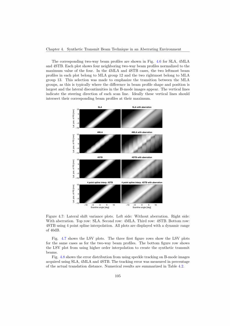
Chapter 4. Synthetic Transmit Beam Technique in an Aberrating Environment
The corresponding two-way beam profiles are shown in Fig. 4.6 for SLA, 4MLAand 4STB. Each plot shows four neighboring two-way beam profiles normalized to themaximum value of the four. In the 4MLA and 4STB cases, the two leftmost beamprofiles in each plot belong to MLA group 12 and the two rightmost belong to MLAgroup 13. This selection was made to emphasize the transition between the MLAgroups, as this is typically where the difference in beam profile shape and position islargest and the lateral discontinuities in the B-mode images appear. The vertical linesindicate the steering direction of each scan line. Ideally these vertical lines shouldintersect their corresponding beam profiles at their maximum.
SLA
Lat.
pos.
of P
S [m
m]
−10
−5
0
5
10SLA with aberration
4MLA
Lat.
pos.
of P
S [m
m]
−10
−5
0
5
104MLA with aberration
4STB
Lat.
pos.
of P
S [m
m]
−10
−5
0
5
104STB with aberration
4 point spline interp. 4STB
Scanline angle [deg]
Lat.
pos.
of P
S [m
m]
−10 −5 0 5 10−10
−5
0
5
104 point spline interp. 4STB with aberration
Scanline angle [deg]−10 −5 0 5 10
Figure 4.7: Lateral shift variance plots. Left side: Without aberration. Right side:With aberration. Top row: SLA. Second row: 4MLA. Third row: 4STB. Bottom row:4STB using 4 point spline interpolation. All plots are displayed with a dynamic rangeof 40dB.
Fig. 4.7 shows the LSV plots. The three first figure rows show the LSV plotsfor the same cases as for the two-way beam profiles. The bottom figure row showsthe LSV plot from using higher order interpolation to create the synthetic transmitbeams.
Fig. 4.8 shows the error distribution from using speckle tracking on B-mode imagesacquired using SLA, 4MLA and 4STB. The tracking error was measured in percentageof the actual translation distance. Numerical results are summarized in Table 4.2.
105
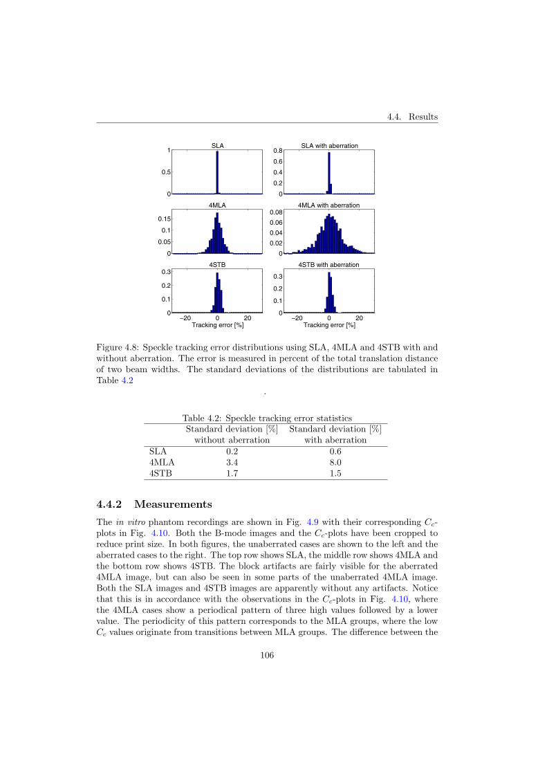
4.4. Results
0
0.5
1SLA
0
0.2
0.4
0.6
0.8SLA with aberration
0
0.05
0.1
0.15
4MLA
0
0.02
0.04
0.06
0.084MLA with aberration
−20 0 200
0.1
0.2
0.34STB
Tracking error [%]−20 0 20
0
0.1
0.2
0.3
4STB with aberration
Tracking error [%]
Figure 4.8: Speckle tracking error distributions using SLA, 4MLA and 4STB with andwithout aberration. The error is measured in percent of the total translation distanceof two beam widths. The standard deviations of the distributions are tabulated inTable 4.2
.
Table 4.2: Speckle tracking error statisticsStandard deviation [%] Standard deviation [%]
without aberration with aberrationSLA 0.2 0.64MLA 3.4 8.04STB 1.7 1.5
4.4.2 Measurements
The in vitro phantom recordings are shown in Fig. 4.9 with their corresponding Cc-plots in Fig. 4.10. Both the B-mode images and the Cc-plots have been cropped toreduce print size. In both figures, the unaberrated cases are shown to the left and theaberrated cases to the right. The top row shows SLA, the middle row shows 4MLA andthe bottom row shows 4STB. The block artifacts are fairly visible for the aberrated4MLA image, but can also be seen in some parts of the unaberrated 4MLA image.Both the SLA images and 4STB images are apparently without any artifacts. Noticethat this is in accordance with the observations in the Cc-plots in Fig. 4.10, wherethe 4MLA cases show a periodical pattern of three high values followed by a lowervalue. The periodicity of this pattern corresponds to the MLA groups, where the lowCc values originate from transitions between MLA groups. The difference between the
106
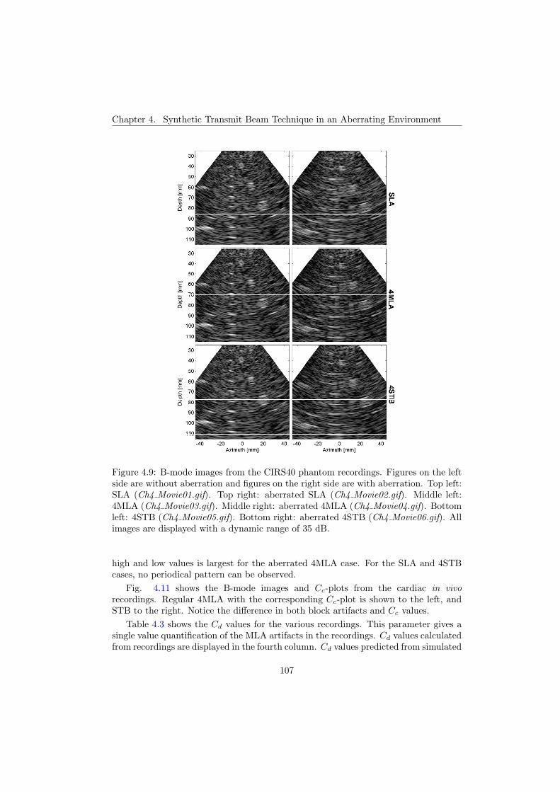
Chapter 4. Synthetic Transmit Beam Technique in an Aberrating Environment
Figure 4.9: B-mode images from the CIRS40 phantom recordings. Figures on the leftside are without aberration and figures on the right side are with aberration. Top left:SLA (Ch4 Movie01.gif). Top right: aberrated SLA (Ch4 Movie02.gif). Middle left:4MLA (Ch4 Movie03.gif). Middle right: aberrated 4MLA (Ch4 Movie04.gif). Bottomleft: 4STB (Ch4 Movie05.gif). Bottom right: aberrated 4STB (Ch4 Movie06.gif). Allimages are displayed with a dynamic range of 35 dB.
high and low values is largest for the aberrated 4MLA case. For the SLA and 4STBcases, no periodical pattern can be observed.
Fig. 4.11 shows the B-mode images and Cc-plots from the cardiac in vivorecordings. Regular 4MLA with the corresponding Cc-plot is shown to the left, andSTB to the right. Notice the difference in both block artifacts and Cc values.
Table 4.3 shows the Cd values for the various recordings. This parameter gives asingle value quantification of the MLA artifacts in the recordings. Cd values calculatedfrom recordings are displayed in the fourth column. Cd values predicted from simulated
107

4.5. Discussion
0
0.5
1
Cor
rela
tion
valu
e
0
0.5
1
Cor
rela
tion
valu
e
20 30 40 500
0.5
1
Cor
rela
tion
valu
e
Scan line correlation pair number20 30 40 50
Scan line correlation pair number
SL
A4M
LA
4ST
B
Figure 4.10: Cc plots from the CIRS40 phantom recordings. Plots correspond to theB-mode images in Fig. 4.9. Plots on the left side are without aberration and plots onthe right side are with aberration. Top: SLA. Middle: 4MLA. Bottom: 4STB.
Table 4.3: Indicator showing differences in correlation, Cd
Acquisition Object Aberration Meas Cd Sim Cd
4MLA Phantom None 18.7 19.84MLA Phantom Silicon 30.0 33.54STB Phantom None -0.4 -1.44STB Phantom Silicon -1.1 -1.24MLA Heart in vivo 25.9 NA4STB Heart in vivo 2.3 NA
two way responses are shown in the last column. Measured and simulated Cd valuesshowed good correspondence. Notice the high values for 4MLA, the increase in the4MLA Cd value from unaberrated to aberrated and the low values for 4STB.
4.5 Discussion
4.5.1 General discussion
Fig. 4.6 shows the simulated two-way beam profiles from the different cases. The toprow shows the beam profiles from using SLA. This case was included as a reference andgold standard. Without aberration, the beam profiles were evenly spaced and equalin shape. This resulted in a straight diagonal structure in the LSV plot shown in Fig.4.7, indicating that this imaging system is shift invariant. As can be seen from thetop left image in Fig. 4.9, the B-mode image obtained using this acquisition method
108
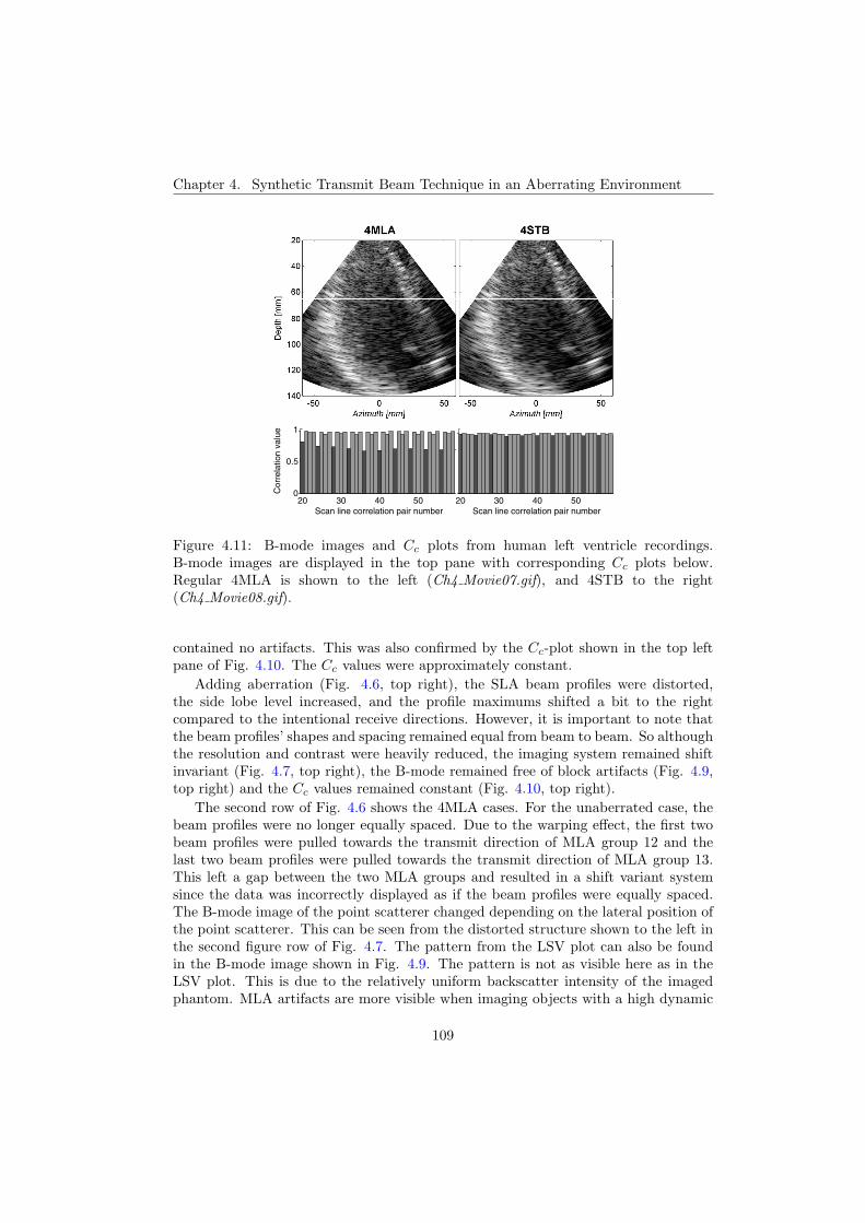
Chapter 4. Synthetic Transmit Beam Technique in an Aberrating Environment
20 30 40 500
0.5
1
Cor
rela
tion
valu
e
Scan line correlation pair number20 30 40 50
Scan line correlation pair number
Figure 4.11: B-mode images and Cc plots from human left ventricle recordings.B-mode images are displayed in the top pane with corresponding Cc plots below.Regular 4MLA is shown to the left (Ch4 Movie07.gif), and 4STB to the right(Ch4 Movie08.gif).
contained no artifacts. This was also confirmed by the Cc-plot shown in the top leftpane of Fig. 4.10. The Cc values were approximately constant.
Adding aberration (Fig. 4.6, top right), the SLA beam profiles were distorted,the side lobe level increased, and the profile maximums shifted a bit to the rightcompared to the intentional receive directions. However, it is important to note thatthe beam profiles’ shapes and spacing remained equal from beam to beam. So althoughthe resolution and contrast were heavily reduced, the imaging system remained shiftinvariant (Fig. 4.7, top right), the B-mode remained free of block artifacts (Fig. 4.9,top right) and the Cc values remained constant (Fig. 4.10, top right).
The second row of Fig. 4.6 shows the 4MLA cases. For the unaberrated case, thebeam profiles were no longer equally spaced. Due to the warping effect, the first twobeam profiles were pulled towards the transmit direction of MLA group 12 and thelast two beam profiles were pulled towards the transmit direction of MLA group 13.This left a gap between the two MLA groups and resulted in a shift variant systemsince the data was incorrectly displayed as if the beam profiles were equally spaced.The B-mode image of the point scatterer changed depending on the lateral position ofthe point scatterer. This can be seen from the distorted structure shown to the left inthe second figure row of Fig. 4.7. The pattern from the LSV plot can also be foundin the B-mode image shown in Fig. 4.9. The pattern is not as visible here as in theLSV plot. This is due to the relatively uniform backscatter intensity of the imagedphantom. MLA artifacts are more visible when imaging objects with a high dynamic
109
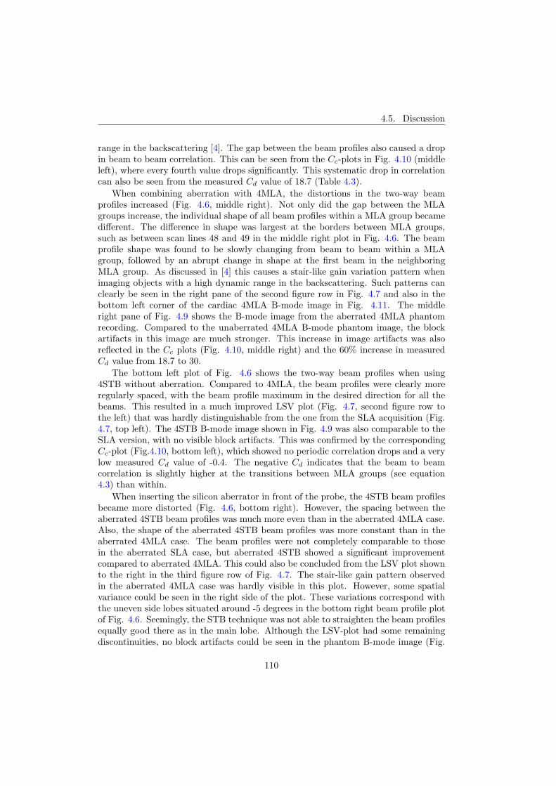
4.5. Discussion
range in the backscattering [4]. The gap between the beam profiles also caused a dropin beam to beam correlation. This can be seen from the Cc-plots in Fig. 4.10 (middleleft), where every fourth value drops significantly. This systematic drop in correlationcan also be seen from the measured Cd value of 18.7 (Table 4.3).
When combining aberration with 4MLA, the distortions in the two-way beamprofiles increased (Fig. 4.6, middle right). Not only did the gap between the MLAgroups increase, the individual shape of all beam profiles within a MLA group becamedifferent. The difference in shape was largest at the borders between MLA groups,such as between scan lines 48 and 49 in the middle right plot in Fig. 4.6. The beamprofile shape was found to be slowly changing from beam to beam within a MLAgroup, followed by an abrupt change in shape at the first beam in the neighboringMLA group. As discussed in [4] this causes a stair-like gain variation pattern whenimaging objects with a high dynamic range in the backscattering. Such patterns canclearly be seen in the right pane of the second figure row in Fig. 4.7 and also in thebottom left corner of the cardiac 4MLA B-mode image in Fig. 4.11. The middleright pane of Fig. 4.9 shows the B-mode image from the aberrated 4MLA phantomrecording. Compared to the unaberrated 4MLA B-mode phantom image, the blockartifacts in this image are much stronger. This increase in image artifacts was alsoreflected in the Cc plots (Fig. 4.10, middle right) and the 60% increase in measuredCd value from 18.7 to 30.
The bottom left plot of Fig. 4.6 shows the two-way beam profiles when using4STB without aberration. Compared to 4MLA, the beam profiles were clearly moreregularly spaced, with the beam profile maximum in the desired direction for all thebeams. This resulted in a much improved LSV plot (Fig. 4.7, second figure row tothe left) that was hardly distinguishable from the one from the SLA acquisition (Fig.4.7, top left). The 4STB B-mode image shown in Fig. 4.9 was also comparable to theSLA version, with no visible block artifacts. This was confirmed by the correspondingCc-plot (Fig.4.10, bottom left), which showed no periodic correlation drops and a verylow measured Cd value of -0.4. The negative Cd indicates that the beam to beamcorrelation is slightly higher at the transitions between MLA groups (see equation4.3) than within.
When inserting the silicon aberrator in front of the probe, the 4STB beam profilesbecame more distorted (Fig. 4.6, bottom right). However, the spacing between theaberrated 4STB beam profiles was much more even than in the aberrated 4MLA case.Also, the shape of the aberrated 4STB beam profiles was more constant than in theaberrated 4MLA case. The beam profiles were not completely comparable to thosein the aberrated SLA case, but aberrated 4STB showed a significant improvementcompared to aberrated 4MLA. This could also be concluded from the LSV plot shownto the right in the third figure row of Fig. 4.7. The stair-like gain pattern observedin the aberrated 4MLA case was hardly visible in this plot. However, some spatialvariance could be seen in the right side of the plot. These variations correspond withthe uneven side lobes situated around -5 degrees in the bottom right beam profile plotof Fig. 4.6. Seemingly, the STB technique was not able to straighten the beam profilesequally good there as in the main lobe. Although the LSV-plot had some remainingdiscontinuities, no block artifacts could be seen in the phantom B-mode image (Fig.
110

Chapter 4. Synthetic Transmit Beam Technique in an Aberrating Environment
4.9, bottom right). This 4STB B-mode image showed similar image quality to theSLA recording. The corresponding Cc-plot shown in Fig. 4.10 showed no periodicdrops in correlation and the measured Cd value was as low as -1.1.
The cardiac 4STB B-mode image and Cc plot is shown to the right in Fig. 4.11.The improvement from using the STB technique compared to regular MLA could easilybe seen both qualitatively in the B-mode images and quantitatively in the Cc plotsand Cd value. By applying the STB technique, the measured Cd value was reducedfrom 25.9 to 2.3.
4.5.2 Simulated and Measured Cd values
Generally the measured and simulated Cd values showed good correspondence. Thisdemonstrates the accuracy of the simulations, and that the measured Cd value providesindirect information about the warping and skewing of the imaging system beamprofiles.
Although the correspondence was good, the simulated Cd value of 4MLA both withand without aberration was slightly higher than the measured. The simulated Cd valuewas calculated from two-way responses of five neighboring scan lines. The two-wayresponses were simulated at focus depth for steering angles around zero degrees. TheCd value of the measurements is calculated from Cc values throughout the imagingsector. The wider beams at the edges of the sector and in the near field results in ahigher Cc and then possibly a lower Cd value.
4.5.3 Speckle Tracking
The results from the speckle tracking are displayed in Fig. 4.8 with tabulated standarddeviations (SD) in Table 4.2. The top figure row shows the tracking error distributionusing SLA. Both without and with aberration, the tracking was found to be veryaccurate for this case. Using four parallel beams the standard deviation of the trackingerror increased noticeably from 0.2% to 3.4% without aberration and from 0.6% to8.0% with aberration. Such increases in error correspond well with the observedincrease in B-mode artifacts from SLA to 4MLA and from 4MLA without aberrationto 4MLA with aberration. Using 4STB (Fig. 4.8 bottom figure row) the standarddeviation of the tracking error was halved without aberration (from 3.5% to 1.7%) andreduced over five times with aberration (from 8.0% to 1.5%). The almost identicaltracking results for 4STB both with and without aberration showed that the speckletracking performance was not affected by aberration when using the STB technique.
4.5.4 Motion Artifacts
Since the STB technique is based on coherent interpolation between data from differenttransmit events, it will be vulnerable to motion artifacts when imaging moving objectssuch as the heart. Motion artifacts cannot easily be observed in Fig. 4.11. Thisis due to the short time delay between the data involved in the STB interpolationand the low velocity of the cardiac tissue compared to the pulse repetition frequency
111
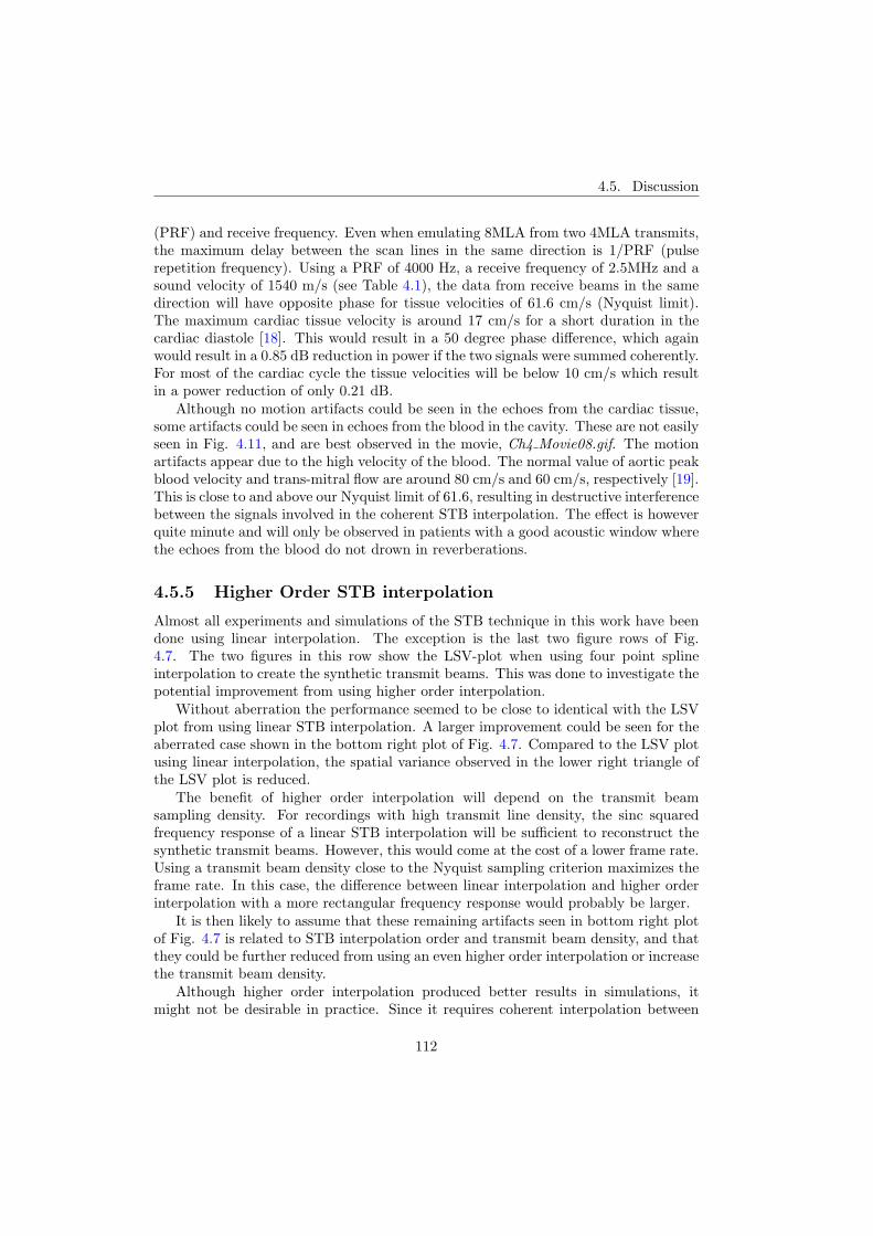
4.5. Discussion
(PRF) and receive frequency. Even when emulating 8MLA from two 4MLA transmits,the maximum delay between the scan lines in the same direction is 1/PRF (pulserepetition frequency). Using a PRF of 4000 Hz, a receive frequency of 2.5MHz and asound velocity of 1540 m/s (see Table 4.1), the data from receive beams in the samedirection will have opposite phase for tissue velocities of 61.6 cm/s (Nyquist limit).The maximum cardiac tissue velocity is around 17 cm/s for a short duration in thecardiac diastole [18]. This would result in a 50 degree phase difference, which againwould result in a 0.85 dB reduction in power if the two signals were summed coherently.For most of the cardiac cycle the tissue velocities will be below 10 cm/s which resultin a power reduction of only 0.21 dB.
Although no motion artifacts could be seen in the echoes from the cardiac tissue,some artifacts could be seen in echoes from the blood in the cavity. These are not easilyseen in Fig. 4.11, and are best observed in the movie, Ch4 Movie08.gif. The motionartifacts appear due to the high velocity of the blood. The normal value of aortic peakblood velocity and trans-mitral flow are around 80 cm/s and 60 cm/s, respectively [19].This is close to and above our Nyquist limit of 61.6, resulting in destructive interferencebetween the signals involved in the coherent STB interpolation. The effect is howeverquite minute and will only be observed in patients with a good acoustic window wherethe echoes from the blood do not drown in reverberations.
4.5.5 Higher Order STB interpolation
Almost all experiments and simulations of the STB technique in this work have beendone using linear interpolation. The exception is the last two figure rows of Fig.4.7. The two figures in this row show the LSV-plot when using four point splineinterpolation to create the synthetic transmit beams. This was done to investigate thepotential improvement from using higher order interpolation.
Without aberration the performance seemed to be close to identical with the LSVplot from using linear STB interpolation. A larger improvement could be seen for theaberrated case shown in the bottom right plot of Fig. 4.7. Compared to the LSV plotusing linear interpolation, the spatial variance observed in the lower right triangle ofthe LSV plot is reduced.
The benefit of higher order interpolation will depend on the transmit beamsampling density. For recordings with high transmit line density, the sinc squaredfrequency response of a linear STB interpolation will be sufficient to reconstruct thesynthetic transmit beams. However, this would come at the cost of a lower frame rate.Using a transmit beam density close to the Nyquist sampling criterion maximizes theframe rate. In this case, the difference between linear interpolation and higher orderinterpolation with a more rectangular frequency response would probably be larger.
It is then likely to assume that these remaining artifacts seen in bottom right plotof Fig. 4.7 is related to STB interpolation order and transmit beam density, and thatthey could be further reduced from using an even higher order interpolation or increasethe transmit beam density.
Although higher order interpolation produced better results in simulations, itmight not be desirable in practice. Since it requires coherent interpolation between
112
Chapter 4. Synthetic Transmit Beam Technique in an Aberrating Environment
data from three or more transmit events, the system would be more vulnerable tomotion artifacts. Also, it would require three or more receive beams in each direction,something that increases the requirements to the hardware. The four point spline STBinterpolation simulated in this work would require 16 parallel beams to produce fouroutput STB beams (if the STB interpolation was done after beamforming).
4.5.6 Considerations on 3D Parallel Beamforming using STB
This study investigated the performance of a STB technique for 2D cardiac phasedarray imaging. If the method is used for 3D imaging, there are some challenges thatone will have to consider. One challenge is motion artifacts. When scanning a volumeinstead of a plane, it is impossible to avoid large time delays between neighboringtransmissions in one of the dimensions. Another issue is the increased hardwarerequirements. If applying the linear interpolation STB technique in both azimuthand elevation directions, the number beams in each receive direction would increasefrom two to four. Hence, a 16 parallel beams system would be required to generate 4output parallel STB scan lines (two in each dimension).
4.6 Conclusion
In this work we compared the STB technique to regular parallel beamforming andsingle line acquisition using several qualitative and quantitative measures. Usinglinear STB interpolation and four parallel receive beams in an aberrating environment,a frame rate of 167 Hz was achieved almost without any visually noticeable blockartifacts in the B-mode images. The improvement from using STB was found to belargest with aberration. Both beam profile regularity, lateral shift invariance, beamto beam correlation consistency and speckle tracking errors improved noticeably inthis case. Higher order STB interpolation was found to further improve lateral shiftinvariance, but might not be desirable due to motion artifacts.
Acknowledgement
The researchers thank GE Vingmed Ultrasound for access to a Vivid 7 ultrasoundscanner.
113

4.6. Conclusion
114

References
[1] B. Lind, J. Nowak, J. Dorph, J. van der Linden, and L. A. Brodin, “Analysisof temporal requirements for myocardial tissue velocity imaging,” Eur JEchocardiogr, vol. 3, pp. 214–9, Sep 2002.
[2] D. P. Shattuck, M. D. Weinshenker, S. W. Smith, and O. T. von Ramm,“Explososcan: A parallel processing technique for high speed ultrasound imagingwith linear phased arrays,” J. Acoust, Soc. Amer., vol. 75, no. 4, pp. 1273–1282,1984.
[3] O. T. von Ramm, S. W. Smith, and H. G. Pavy, “High-speed ultrasoundvolumetric imaging system – part ii: Parallel processing and image display,”IEEE transactions on ultrasonics, ferroelectrics, and frequency control, vol. 38,March 1991.
[4] T. Bjastad, S. A. Aase, and H. Torp, “The impact of aberration on high framerate cardiac b-mode imaging,” IEEE transactions on ultrasonics, ferroelectrics,and frequency control, vol. 54, January 2007.
[5] T. Hergum, T. Bjastad, K. Kristoffersen, and H. Torp, “Parallel beamformingusing synthetic transmit beams,” IEEE transactions on ultrasonics, ferroelectrics,and frequency control, vol. 54, February 2007.
[6] J. J. Dahl, G. F. Pinton, M. L. Palmeri, V. Agrawal, K. R. Nightingale, andG. E. Trahey, “A parallel tracking method for acoustic radiation force impulseimaging,” IEEE transactions on ultrasonics, ferroelectrics, and frequency control,vol. 54, February 2007.
[7] L. J. Augustine, “High resolution multiline ultrasonic beamformer.” U.S. Patent4.644.795, 1985.
[8] G. L. Holley and I. M. Guracar, “Ultrasound multi-beam distortion correctionsystem and method.” U.S. Patent 5.779.640, July 14 1998.
[9] D.-L. D. Liu, J. C. Lazenby, Z. Banjanin, and B. A. McDermot, “System andmethod for reduction of parallel beamforming artifacts.” U.S. Patent 6.447.452,Sep. 10 2002.
115
References
[10] T. J. Hunt, B. M. Herrick, K. K. Robertson, and J. M. Ziel, “Ultrasonic imagingsystem using line splicing and parallel receive beam formation.” U.S. patent5.462.057, Oct. 31 1995.
[11] M. Bernard J. Savord, Andover, “Method and apparatus for increasing the framerate and resolution of a phased array imaging system.” U.S. patent 5.318.033,1992.
[12] T. L. Szabo, Diagnostic Ultrasound Imaging: Inside Out. Elsevier AcademicPress, 2004.
[13] R. F. Wagner, S. W. Smith, J. M. Sandrik, and H. Lopez, “Statistics of specklein ultrasound b-scans,” IEEE transactions on ultrasonics, ferroelectrics, andfrequency control, 1983.
[14] J. D’hooge, Myocardial Imaging: Tissue Doppler and Speckle Tracking,ch. Principles and different techniques for speckle tracking, pp. 17–25. BlackwellPublishing, 2007.
[15] J. A. Jensen and N. B. Svendsen, “Calculation of pressure fields fromarbitrarily shaped, apodized, and excited ultrasound transducers,” IEEE Trans.Ultrason.,Ferroelec., Freq. Contr., 1992.
[16] T. Johansen, B. Angelsen, and W. Nordhøy, “Phase aberrations - experimentsand simulations,” Proceedings of the 23rd Scandinavian Symposium on PhysicalAcoustics, 2000.
[17] L. M. Hinkelman, T. L. Szabo, and R. C. Waag, “Measurements of ultrasonicpulse distortion produced by human chest wall,” J. Acoust. Soc. Am., 1997.
[18] G. Sutherland, L. Hatle, P. Claus, L. Herbots, and J. Separovic, DopplerMyocardial Imaging, ch. Normal Data, pp. 49–102. BSWK, 2006.
[19] J. Rinaldi and B. Diebold, Cardiac Ultrasound, ch. Normal Intra Cardiac DopplerFlows, pp. 141–153. Churchill Livingstone, 1993.
116

Chapter 5
Single Pulse Tissue Dopplerusing Synthetic TransmitBeamsT. Bjastad and H. TorpDept. Circulation and Medical Imaging, NTNU
Tissue Doppler Imaging (TDI) is a common technique for investigatingmyocardial function. Typically B-mode data and TDI data are recorded usingseparate acquisitions and combined into a single color overlaid image. In thiswork, we present a novel method for TDI imaging, where both TDI and B-mode are created from the same acquisition. Velocities are calculated from thephase shift between neighboring transmit events in the B-mode scan (hencethe name Single Pulse Tissue Doppler, SPTD). Using a novel transmit beaminterleaving pattern, this method provides TDI and B-mode at the same highframe rate with an adjustable Nyquist velocity limit.Through simulations and measurements this work investigates the bias andvariance of the SPTD velocities and compares the estimates to those of theconventional TDI autocorrelation estimation method.The results showed that the method has a larger bias and variance inthe velocity estimates than conventional TDI. However, by applying biascompensation, the accuracy of the SPTD velocity estimates was close to thatof regular TDI. Using SPTD the whole left ventricle was imaged within a 65degree sector at a frame rate of 110 frames per second.
5.1 Introduction
Tissue Doppler imaging was first introduced by McDicken et al in 1992 [1]. Since then,TDI has become a common imaging modality among cardiologists since it enablesquantitative evaluation of cardiac tissue function. Due to rapid tissue deformation,high frame rate is a desired property in cardiac TDI. According to [2], frame ratesabove 100 Hz are required to accurately resolve all myocardial mechanical events
117

5.1. Introduction
using tissueDoppler. However, the full frequency spectrum of cardiac motion containscomponents up to 100 Hertz [3, 4]. Detecting these components would require framerates above 200 Hertz. Combined with high frame rate it is also desirable to have awide sector. One specific example is when assessing asynchrony between cardiac walls[5, 6]. It is then advantageous to image the whole left ventricle in one field of view.High frame rate and large field of view are, however, conflicting properties. Increasingone of them will typically reduce the other. The factor determining the frame ratein cardiac TDI, is the number of transmit beams per image frame. Simply reducingthe number of transmit beams will also reduce the imaging sector. If reducing theamount of transmit beams and at the same time maintaining a large field of view,the transmit beams will have to be wider. This is done by reducing the transmitaperture, something that reduces both penetration and lateral resolution. To avoidwider receive beams as well, multiple line acquisition (MLA) can be applied. Severalnarrow receive beams are then formed for each transmit event [7, 8]. However, usingstraightforward MLA the B-mode images will suffer from block like image artifacts [9].In [10] it is shown that these block artifacts can be suppressed by creating synthetictransmit beams (STB) in each receive direction. The synthetic transmit beams werecreated by receiving in the same direction in neighboring transmit events.
Traditional TDI requires separate acquisitions for B-mode and Doppler images.One frame of B-mode is acquired for each Doppler frame. A possible approach toincrease overall TDI frame rate is then to separately decrease the B-mode framerate [11]. For example one B-mode frame for every second Doppler frame. Thisdoes, however, result in a lower B-mode temporal resolution and a temporal mismatchbetween the displayed B-mode image and the overlaid velocities.
In [12] a method for continuous acquisition high frame rate tissue Doppler isdescribed. The velocities are then estimated from phase shifts between consecutiveframes. This eliminates the need for a separate tissue Doppler acquisition, but, to avoidaliasing, the number of transmit beams have to be kept low. Hence, this method ismost suitable for narrow sector imaging.
US patent 6589177 B1 [13] sketches a method for using the phase shift betweenneighboring transmit beams for both B-flow and B-mode. This technique may alsobe applied to tissue Doppler, but the patent does not address the problem of parallelbeamforming artifacts in the B-mode. Neither does it provide any scheme for adjustingthe Nyquist limit without reducing the frame rate, which is necessary for cardiac TDI.
In our single pulse tissue Doppler method (SPTD), we apply the STB technique(Synthetic Transmit Beam, [10, 14]) to achieve high frame rate B-mode withsuppressed image artifacts. Using the STB implementation of [10], each scan lineis created from two neighboring transmit events with identical receive direction. Theidea of SPTD is to estimate the phase shift between these two receive beams in thesame direction. In this way one can achieve both high frame rate B-mode and tissueDoppler from a single acquisition. We also suggest a novel transmit beam interleavingpattern to adjust the time delay between the overlapping receive beams. This allowsadjustments of the Nyquist velocity limit without reducing the frame rate.
The paper is organized as follows. Section 5.2 contains theory on the SPTD methodand the applied interleaving pattern. This chapter also contains a brief explanation on
118
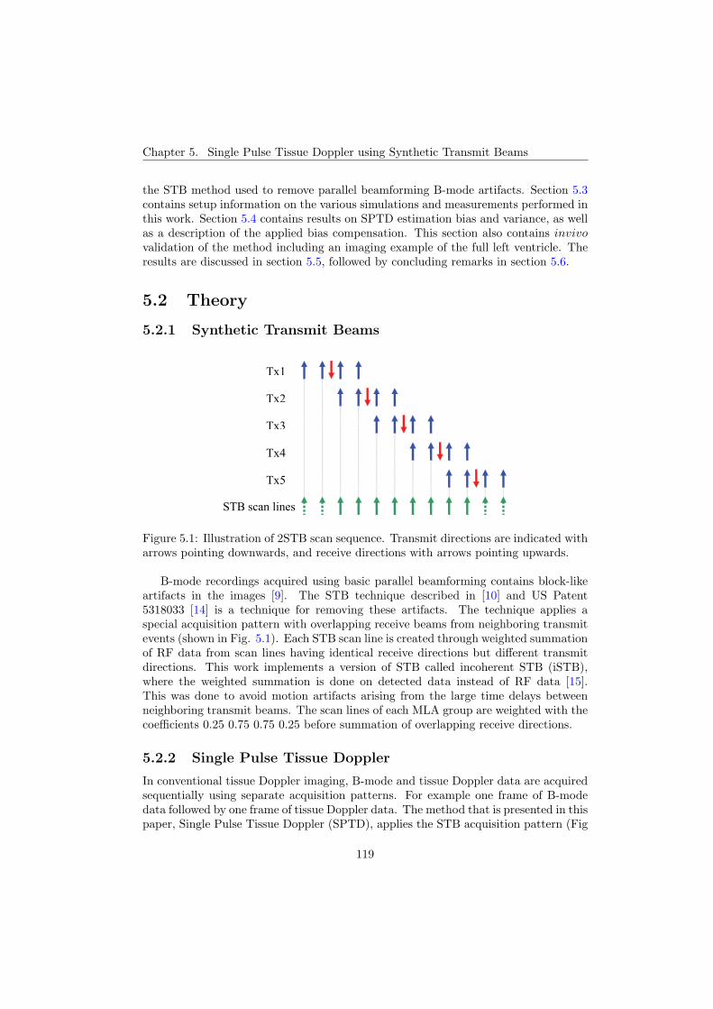
Chapter 5. Single Pulse Tissue Doppler using Synthetic Transmit Beams
the STB method used to remove parallel beamforming B-mode artifacts. Section 5.3contains setup information on the various simulations and measurements performed inthis work. Section 5.4 contains results on SPTD estimation bias and variance, as wellas a description of the applied bias compensation. This section also contains invivovalidation of the method including an imaging example of the full left ventricle. Theresults are discussed in section 5.5, followed by concluding remarks in section 5.6.
5.2 Theory
5.2.1 Synthetic Transmit Beams
Tx1
Tx2
Tx3
Tx4
Tx5
STB scan lines
Figure 5.1: Illustration of 2STB scan sequence. Transmit directions are indicated witharrows pointing downwards, and receive directions with arrows pointing upwards.
B-mode recordings acquired using basic parallel beamforming contains block-likeartifacts in the images [9]. The STB technique described in [10] and US Patent5318033 [14] is a technique for removing these artifacts. The technique applies aspecial acquisition pattern with overlapping receive beams from neighboring transmitevents (shown in Fig. 5.1). Each STB scan line is created through weighted summationof RF data from scan lines having identical receive directions but different transmitdirections. This work implements a version of STB called incoherent STB (iSTB),where the weighted summation is done on detected data instead of RF data [15].This was done to avoid motion artifacts arising from the large time delays betweenneighboring transmit beams. The scan lines of each MLA group are weighted with thecoefficients 0.25 0.75 0.75 0.25 before summation of overlapping receive directions.
5.2.2 Single Pulse Tissue Doppler
In conventional tissue Doppler imaging, B-mode and tissue Doppler data are acquiredsequentially using separate acquisition patterns. For example one frame of B-modedata followed by one frame of tissue Doppler data. The method that is presented in thispaper, Single Pulse Tissue Doppler (SPTD), applies the STB acquisition pattern (Fig
119
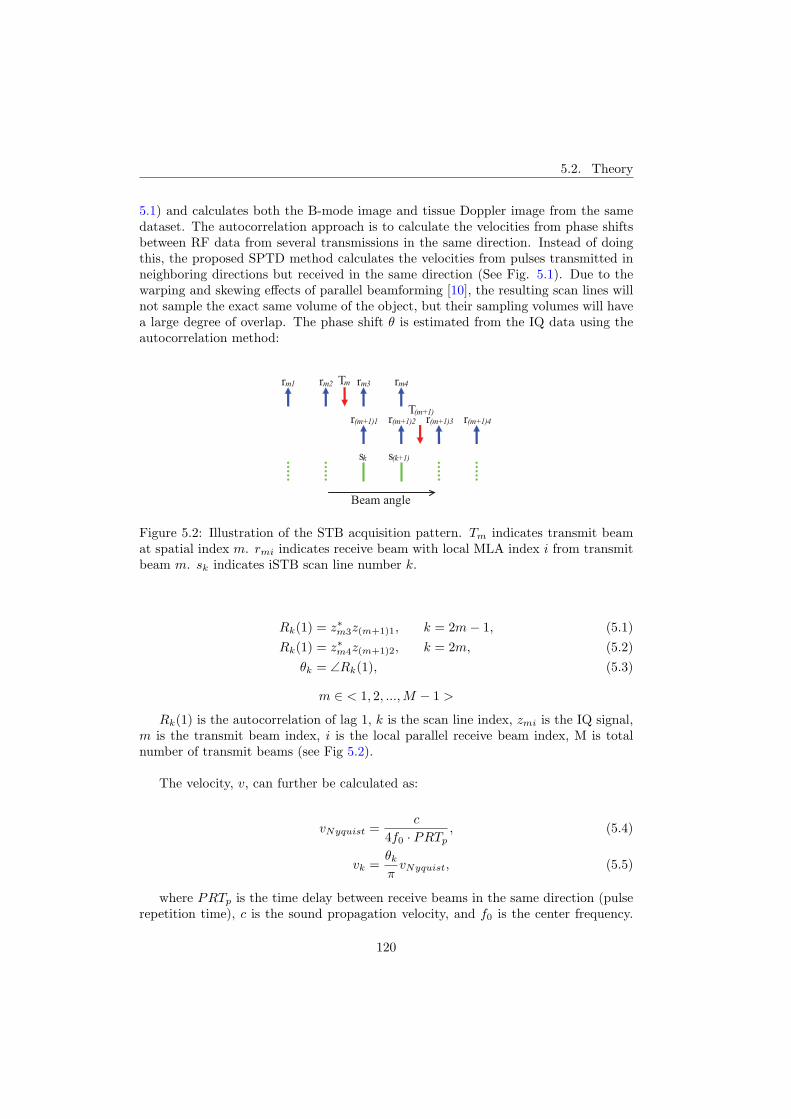
5.2. Theory
5.1) and calculates both the B-mode image and tissue Doppler image from the samedataset. The autocorrelation approach is to calculate the velocities from phase shiftsbetween RF data from several transmissions in the same direction. Instead of doingthis, the proposed SPTD method calculates the velocities from pulses transmitted inneighboring directions but received in the same direction (See Fig. 5.1). Due to thewarping and skewing effects of parallel beamforming [10], the resulting scan lines willnot sample the exact same volume of the object, but their sampling volumes will havea large degree of overlap. The phase shift θ is estimated from the IQ data using theautocorrelation method:
rm1
r(m+1)2
s(k+1)sk
r(m+1)1 r(m+1)3 r(m+1)4T(m+1)
Tmrm2 rm3 rm4
Beam angle
Figure 5.2: Illustration of the STB acquisition pattern. Tm indicates transmit beamat spatial index m. rmi indicates receive beam with local MLA index i from transmitbeam m. sk indicates iSTB scan line number k.
Rk(1) = z∗m3z(m+1)1, k = 2m − 1, (5.1)Rk(1) = z∗m4z(m+1)2, k = 2m, (5.2)
θk = ∠Rk(1), (5.3)
m ∈ < 1, 2, ...,M − 1 >
Rk(1) is the autocorrelation of lag 1, k is the scan line index, zmi is the IQ signal,m is the transmit beam index, i is the local parallel receive beam index, M is totalnumber of transmit beams (see Fig 5.2).
The velocity, v, can further be calculated as:
vNyquist =c
4f0 · PRTp, (5.4)
vk =θk
πvNyquist, (5.5)
where PRTp is the time delay between receive beams in the same direction (pulserepetition time), c is the sound propagation velocity, and f0 is the center frequency.
120
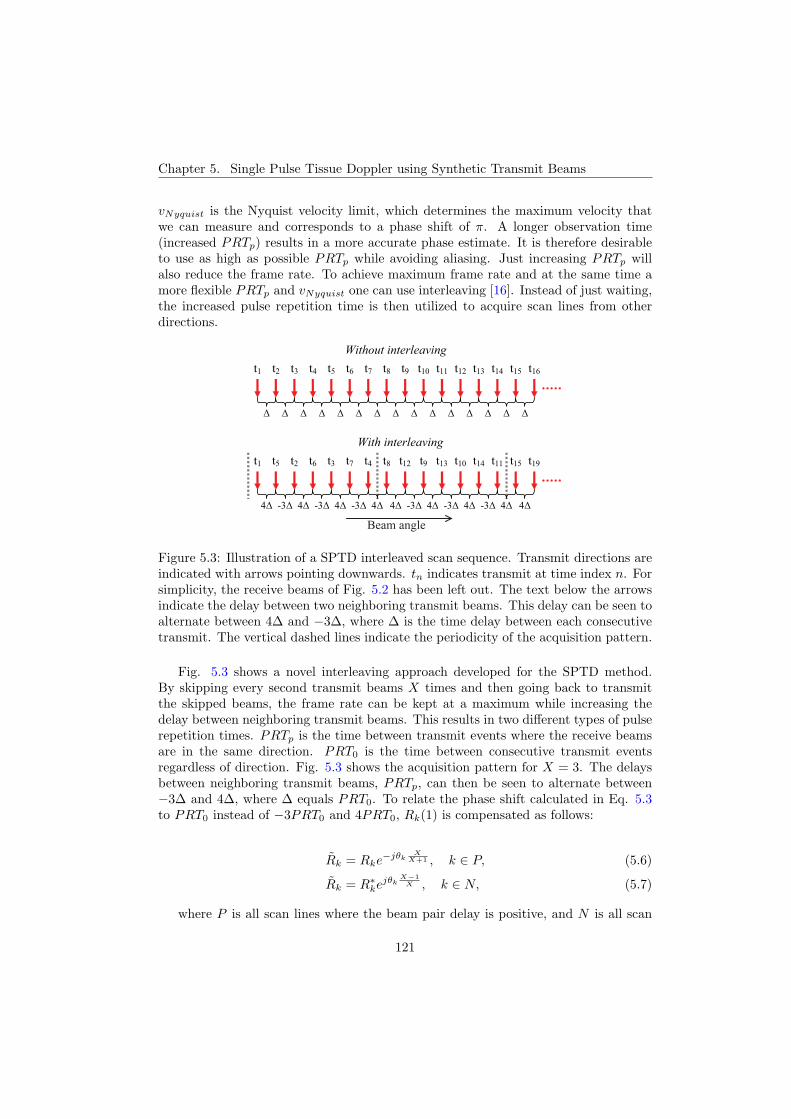
Chapter 5. Single Pulse Tissue Doppler using Synthetic Transmit Beams
vNyquist is the Nyquist velocity limit, which determines the maximum velocity thatwe can measure and corresponds to a phase shift of π. A longer observation time(increased PRTp) results in a more accurate phase estimate. It is therefore desirableto use as high as possible PRTp while avoiding aliasing. Just increasing PRTp willalso reduce the frame rate. To achieve maximum frame rate and at the same time amore flexible PRTp and vNyquist one can use interleaving [16]. Instead of just waiting,the increased pulse repetition time is then utilized to acquire scan lines from otherdirections.
t1 t2 t3 t4 t5 t6
Without interleaving
With interleaving
t7 t8 t9 t10 t11 t12 t13 t14 t15 t16
t1 t2 t3 t4 t5 t6 t7 t8 t9 t10 t11 t12 t13 t14 t15 t19
4Δ -3Δ 4Δ -3Δ 4Δ -3Δ 4Δ 4Δ -3Δ 4Δ -3Δ 4Δ -3Δ 4Δ 4Δ
Δ Δ Δ Δ Δ Δ Δ Δ Δ Δ Δ Δ Δ Δ Δ
Beam angle
Figure 5.3: Illustration of a SPTD interleaved scan sequence. Transmit directions areindicated with arrows pointing downwards. tn indicates transmit at time index n. Forsimplicity, the receive beams of Fig. 5.2 has been left out. The text below the arrowsindicate the delay between two neighboring transmit beams. This delay can be seen toalternate between 4Δ and −3Δ, where Δ is the time delay between each consecutivetransmit. The vertical dashed lines indicate the periodicity of the acquisition pattern.
Fig. 5.3 shows a novel interleaving approach developed for the SPTD method.By skipping every second transmit beams X times and then going back to transmitthe skipped beams, the frame rate can be kept at a maximum while increasing thedelay between neighboring transmit beams. This results in two different types of pulserepetition times. PRTp is the time between transmit events where the receive beamsare in the same direction. PRT0 is the time between consecutive transmit eventsregardless of direction. Fig. 5.3 shows the acquisition pattern for X = 3. The delaysbetween neighboring transmit beams, PRTp, can then be seen to alternate between−3Δ and 4Δ, where Δ equals PRT0. To relate the phase shift calculated in Eq. 5.3to PRT0 instead of −3PRT0 and 4PRT0, Rk(1) is compensated as follows:
Rk = Rke−jθkX
X+1 , k ∈ P, (5.6)
Rk = R∗kejθk
X−1X , k ∈ N, (5.7)
where P is all scan lines where the beam pair delay is positive, and N is all scan
121
5.3. Setup
lines where the beam pair delay is negative. After this beam pair delay compensation,velocities can be calculated using Eq. 5.4 and 5.5 with PRT0 instead of PRTp.
From Fig 5.3, it can be seen that the acquisition pattern repeats after everyseventh transmit beam (indicated by the vertical dashed lines in the figure). Periodicacquisition patterns for all delay combinations of −X · PRT0 and (X + 1) · PRT0 canbe constructed. Their period, Ti is given by:
Ti = 2X + 1. (5.8)
Using such interleaving patterns, the positive and negative delay beam pairs willhave different Nyquist limit. Substituting PRTp in Eq. 5.4 with (X + 1) · PRT0 andX · PRT0 gives:
vNyquistP=
c
(X + 1) · PRT0 · 4f0, (5.9)
vNyquistN=
c
X · PRT0 · 4f0. (5.10)
where vNyquistPis the Nyquist limit for positive delay beam pairs and vNyquistN
for negative delay beam pairs. Hence, the Nyquist limit of negative delay beam pairswill be (X + 1)/X times higher than for the positive delay beam pairs.
5.2.3 Inter scan line correlation
Assuming Rayleigh scattering conditions, the authors in [17] show that theautocorrelation for a complex amplitude process equals the scaled autocorrelationof the two-way response. Both conventional TDI and SPTD use autocorrelation toestimate phase shifts between consecutive transmit events. For conventional TDI,the two-way response of the consecutive transmit events are identical, since thetransmit and receive direction are the same. Hence, the phase estimate for stationarytargets will be consistently zero at all locations using conventional TDI. Using SPTD,the receive directions of consecutive transmit events are identical, but the transmitdirections are different. The two-way responses will therefore not be completelycorrelated. This decorrelation will result in two things. Firstly the expected valueof the phase estimate might not be zero for stationary targets. Secondly, the phaseestimate will vary with position for stationary targets. In other words, the SPTDphase estimate will have a variance and might have a bias.
5.3 Setup
All recordings were made using a modified GE Vingmed System 7 scanner capable ofrecording IQ data and a M3S phased array probe. The main acquisition parameters arelisted in Table 5.1. With the exception of the narrow sector recordings, the parametersspecified in this table were used in all the recordings and simulations. Changes inacquisition parameters for the narrow sector recordings are listed in Table 5.2.
122
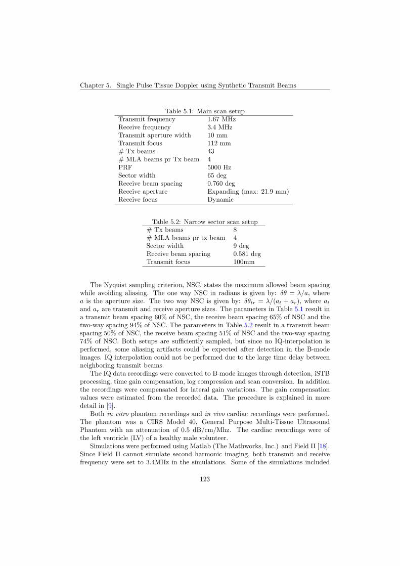
Chapter 5. Single Pulse Tissue Doppler using Synthetic Transmit Beams
Table 5.1: Main scan setupTransmit frequency 1.67 MHzReceive frequency 3.4 MHzTransmit aperture width 10 mmTransmit focus 112 mm# Tx beams 43# MLA beams pr Tx beam 4PRF 5000 HzSector width 65 degReceive beam spacing 0.760 degReceive aperture Expanding (max: 21.9 mm)Receive focus Dynamic
Table 5.2: Narrow sector scan setup# Tx beams 8# MLA beams pr tx beam 4Sector width 9 degReceive beam spacing 0.581 degTransmit focus 100mm
The Nyquist sampling criterion, NSC, states the maximum allowed beam spacingwhile avoiding aliasing. The one way NSC in radians is given by: δθ = λ/a, wherea is the aperture size. The two way NSC is given by: δθtr = λ/(at + ar), where at
and ar are transmit and receive aperture sizes. The parameters in Table 5.1 result ina transmit beam spacing 60% of NSC, the receive beam spacing 65% of NSC and thetwo-way spacing 94% of NSC. The parameters in Table 5.2 result in a transmit beamspacing 50% of NSC, the receive beam spacing 51% of NSC and the two-way spacing74% of NSC. Both setups are sufficiently sampled, but since no IQ-interpolation isperformed, some aliasing artifacts could be expected after detection in the B-modeimages. IQ interpolation could not be performed due to the large time delay betweenneighboring transmit beams.
The IQ data recordings were converted to B-mode images through detection, iSTBprocessing, time gain compensation, log compression and scan conversion. In additionthe recordings were compensated for lateral gain variations. The gain compensationvalues were estimated from the recorded data. The procedure is explained in moredetail in [9].
Both in vitro phantom recordings and in vivo cardiac recordings were performed.The phantom was a CIRS Model 40, General Purpose Multi-Tissue UltrasoundPhantom with an attenuation of 0.5 dB/cm/Mhz. The cardiac recordings were ofthe left ventricle (LV) of a healthy male volunteer.
Simulations were performed using Matlab (The Mathworks, Inc.) and Field II [18].Since Field II cannot simulate second harmonic imaging, both transmit and receivefrequency were set to 3.4MHz in the simulations. Some of the simulations included
123
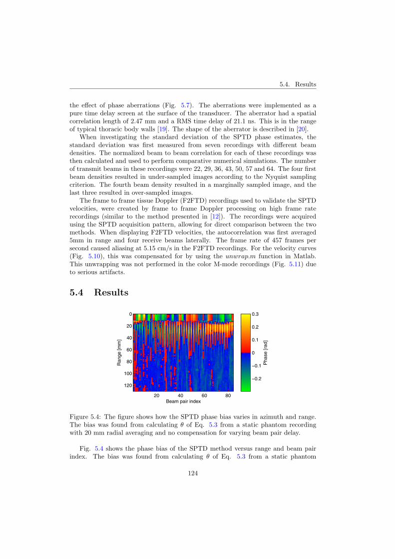
5.4. Results
the effect of phase aberrations (Fig. 5.7). The aberrations were implemented as apure time delay screen at the surface of the transducer. The aberrator had a spatialcorrelation length of 2.47 mm and a RMS time delay of 21.1 ns. This is in the rangeof typical thoracic body walls [19]. The shape of the aberrator is described in [20].
When investigating the standard deviation of the SPTD phase estimates, thestandard deviation was first measured from seven recordings with different beamdensities. The normalized beam to beam correlation for each of these recordings wasthen calculated and used to perform comparative numerical simulations. The numberof transmit beams in these recordings were 22, 29, 36, 43, 50, 57 and 64. The four firstbeam densities resulted in under-sampled images according to the Nyquist samplingcriterion. The fourth beam density resulted in a marginally sampled image, and thelast three resulted in over-sampled images.
The frame to frame tissue Doppler (F2FTD) recordings used to validate the SPTDvelocities, were created by frame to frame Doppler processing on high frame raterecordings (similar to the method presented in [12]). The recordings were acquiredusing the SPTD acquisition pattern, allowing for direct comparison between the twomethods. When displaying F2FTD velocities, the autocorrelation was first averaged5mm in range and four receive beams laterally. The frame rate of 457 frames persecond caused aliasing at 5.15 cm/s in the F2FTD recordings. For the velocity curves(Fig. 5.10), this was compensated for by using the unwrap.m function in Matlab.This unwrapping was not performed in the color M-mode recordings (Fig. 5.11) dueto serious artifacts.
5.4 Results
Beam pair index
Ran
ge [m
m]
20 40 60 80
0
20
40
60
80
100
120
Pha
se [r
ad]
−0.2
−0.1
0
0.1
0.2
0.3
Figure 5.4: The figure shows how the SPTD phase bias varies in azimuth and range.The bias was found from calculating θ of Eq. 5.3 from a static phantom recordingwith 20 mm radial averaging and no compensation for varying beam pair delay.
Fig. 5.4 shows the phase bias of the SPTD method versus range and beam pairindex. The bias was found from calculating θ of Eq. 5.3 from a static phantom
124

Chapter 5. Single Pulse Tissue Doppler using Synthetic Transmit Beams
recording using the SPTD acquisition pattern. θ was averaged over approximately20 mm in the radial direction, and no compensation for varying beam pair delay wasdone. Ideally θ should be zero at all locations in a recording of at static phantom, but,as the figure shows, θ had a systematic pattern in the lateral direction which changedwith depth.
−0.4
−0.2
0
0.2
0.4Range = 22.9 mm
Pha
se [r
ad]
−0.4
−0.2
0
0.2
0.4Range = 69.2 mm
20 40 60 80−0.4
−0.2
0
0.2
0.4
Beam idx
Pha
se [r
ad]
20 40 60 80−0.4
−0.2
0
0.2
0.4
Beam idx
Figure 5.5: Comparison of simulated and measured phase bias. Top figure row showsthe measured phase bias from static phantom recordings and bottom row shows thesimulated phase bias as a function of beam pair index. Left figure column shows resultsfrom a range of 22.9 mm and the right figure column from a range of 69.2mm. Biasfrom beam pairs with positive delays are shown in red and negative delays in blue.
The top row of Fig. 5.5 shows plots of the measured phase bias at ranges 22.9mm and 69.2 mm. The same phase bias should also be found from calculating thephase shift between the two-way responses of the scan lines at these depths [17]. Thephase shifts found from simulating the two way responses of all scan lines at the samedepths is shown in the bottom figure row of Fig. 5.5. These simulated phase shiftscorresponded well with the measured ones. Notice the diagonal symmetry, and thatthe bias oscillates around a laterally slowly varying value.
The reason for this scan line dependent bias was found from investigating thelateral phase variation of the transmitted pressure field. Fig. 5.6 shows simulations oflateral phase variations across the transmit beam for ranges 22.9 mm and 69.2 mm.The first and second figure row show the transmitted pressure field and the transmitbeam profile, respectively. The third figure row shows the actual phase variations.The same plots are repeated for range 69.2 mm in figure rows four to six. For bothranges the phase shift varied significantly with receive beam positions (indicated bythe thin vertical lines). This resulted in phase shifts between the data from differentparallel beams. The phase variation were largest at the 22.9 mm range. Notice thatthe phase profile was symmetrical for zero degree steering angles and asymmetricalwhen steering to either side. Also, the phase profiles were mirrored versions of eachother when comparing positive and negative steering angles. This caused the s-shape
125
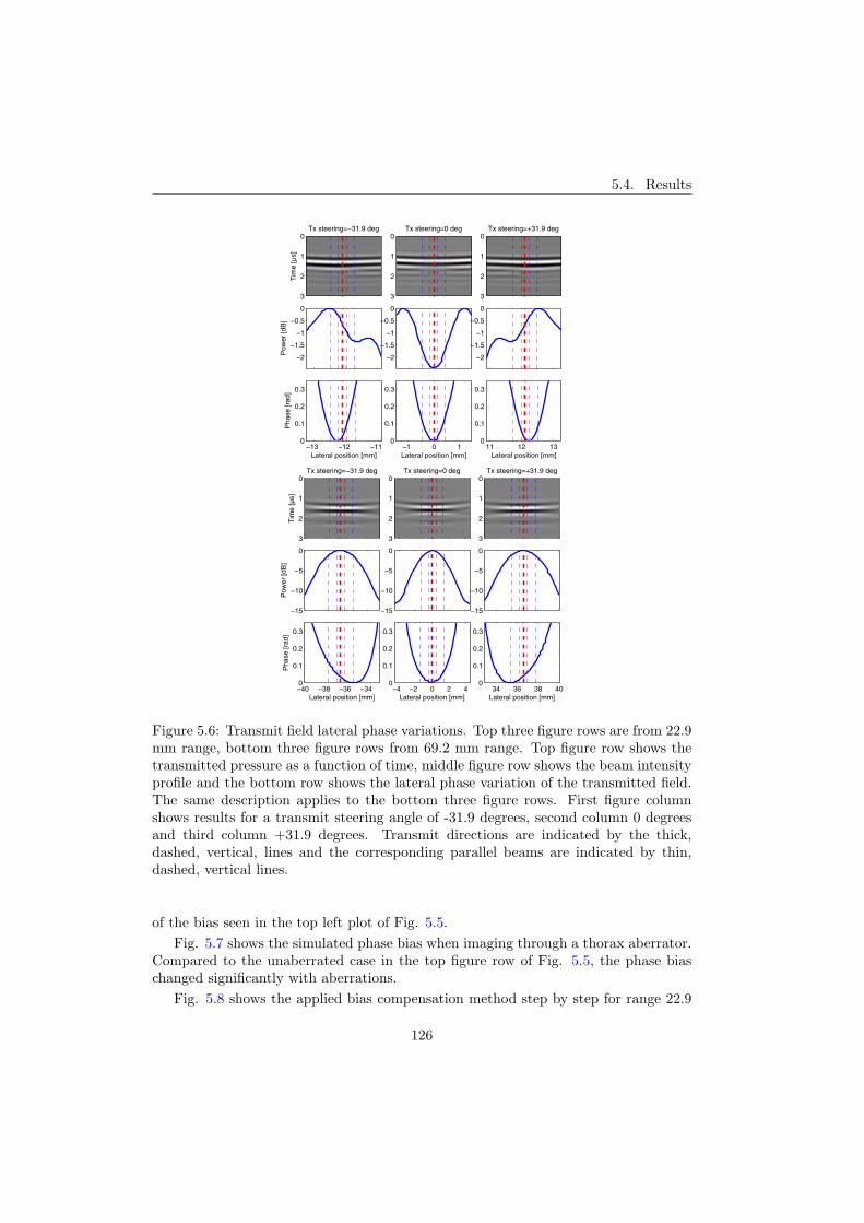
5.4. Results
Tx steering=−31.9 deg
Tim
e [µ
s]
0
1
2
3
Tx steering=0 deg0
1
2
3
Tx steering=+31.9 deg0
1
2
3
−2
−1.5
−1
−0.5
0
Pow
er [d
B]
−2
−1.5
−1
−0.5
0
−2
−1.5
−1
−0.5
0
−13 −12 −110
0.1
0.2
0.3
Lateral position [mm]
Pha
se [r
ad]
−1 0 10
0.1
0.2
0.3
Lateral position [mm]11 12 13
0
0.1
0.2
0.3
Lateral position [mm]
Tx steering=−31.9 deg
Tim
e [µ
s]
0
1
2
3
Tx steering=0 deg0
1
2
3
Tx steering=+31.9 deg0
1
2
3
−15
−10
−5
0
Pow
er [d
B]
−15
−10
−5
0
−15
−10
−5
0
−40 −38 −36 −340
0.1
0.2
0.3
Lateral position [mm]
Pha
se [r
ad]
−4 −2 0 2 40
0.1
0.2
0.3
Lateral position [mm]34 36 38 40
0
0.1
0.2
0.3
Lateral position [mm]
Figure 5.6: Transmit field lateral phase variations. Top three figure rows are from 22.9mm range, bottom three figure rows from 69.2 mm range. Top figure row shows thetransmitted pressure as a function of time, middle figure row shows the beam intensityprofile and the bottom row shows the lateral phase variation of the transmitted field.The same description applies to the bottom three figure rows. First figure columnshows results for a transmit steering angle of -31.9 degrees, second column 0 degreesand third column +31.9 degrees. Transmit directions are indicated by the thick,dashed, vertical, lines and the corresponding parallel beams are indicated by thin,dashed, vertical lines.
of the bias seen in the top left plot of Fig. 5.5.Fig. 5.7 shows the simulated phase bias when imaging through a thorax aberrator.
Compared to the unaberrated case in the top figure row of Fig. 5.5, the phase biaschanged significantly with aberrations.
Fig. 5.8 shows the applied bias compensation method step by step for range 22.9
126
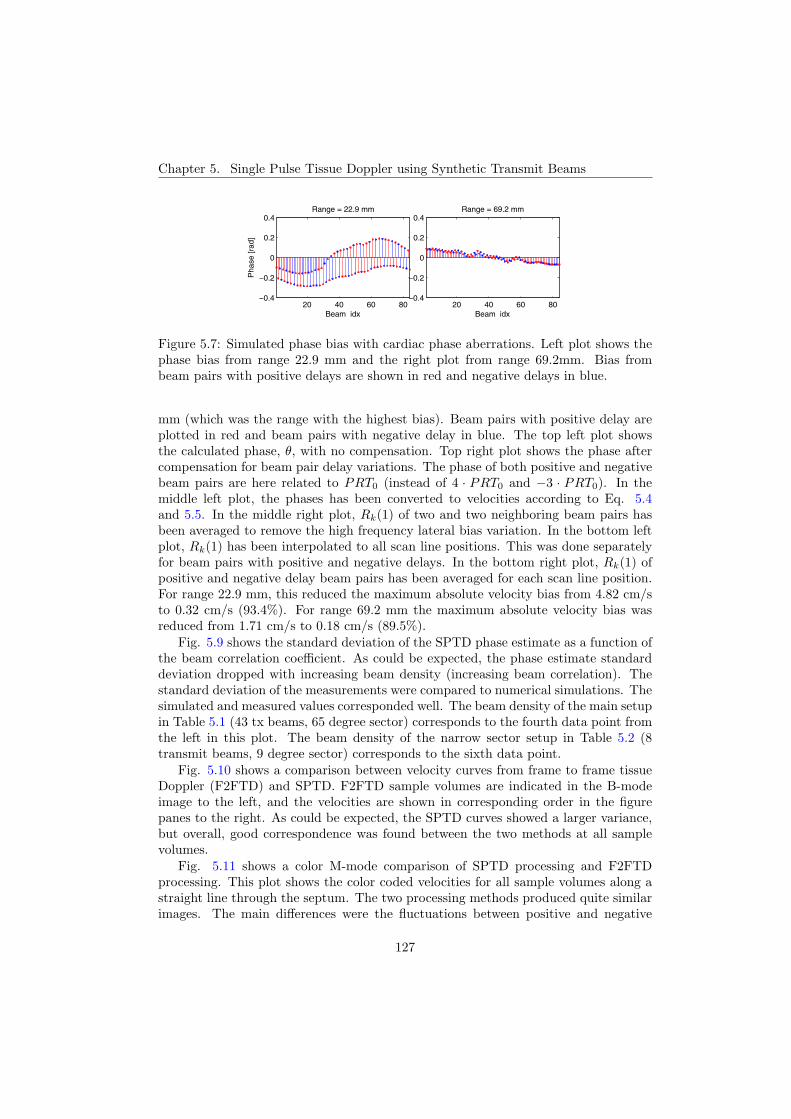
Chapter 5. Single Pulse Tissue Doppler using Synthetic Transmit Beams
20 40 60 80−0.4
−0.2
0
0.2
0.4
Beam idx
Pha
se [r
ad]
Range = 22.9 mm
20 40 60 80−0.4
−0.2
0
0.2
0.4
Beam idx
Range = 69.2 mm
Figure 5.7: Simulated phase bias with cardiac phase aberrations. Left plot shows thephase bias from range 22.9 mm and the right plot from range 69.2mm. Bias frombeam pairs with positive delays are shown in red and negative delays in blue.
mm (which was the range with the highest bias). Beam pairs with positive delay areplotted in red and beam pairs with negative delay in blue. The top left plot showsthe calculated phase, θ, with no compensation. Top right plot shows the phase aftercompensation for beam pair delay variations. The phase of both positive and negativebeam pairs are here related to PRT0 (instead of 4 · PRT0 and −3 · PRT0). In themiddle left plot, the phases has been converted to velocities according to Eq. 5.4and 5.5. In the middle right plot, Rk(1) of two and two neighboring beam pairs hasbeen averaged to remove the high frequency lateral bias variation. In the bottom leftplot, Rk(1) has been interpolated to all scan line positions. This was done separatelyfor beam pairs with positive and negative delays. In the bottom right plot, Rk(1) ofpositive and negative delay beam pairs has been averaged for each scan line position.For range 22.9 mm, this reduced the maximum absolute velocity bias from 4.82 cm/sto 0.32 cm/s (93.4%). For range 69.2 mm the maximum absolute velocity bias wasreduced from 1.71 cm/s to 0.18 cm/s (89.5%).
Fig. 5.9 shows the standard deviation of the SPTD phase estimate as a function ofthe beam correlation coefficient. As could be expected, the phase estimate standarddeviation dropped with increasing beam density (increasing beam correlation). Thestandard deviation of the measurements were compared to numerical simulations. Thesimulated and measured values corresponded well. The beam density of the main setupin Table 5.1 (43 tx beams, 65 degree sector) corresponds to the fourth data point fromthe left in this plot. The beam density of the narrow sector setup in Table 5.2 (8transmit beams, 9 degree sector) corresponds to the sixth data point.
Fig. 5.10 shows a comparison between velocity curves from frame to frame tissueDoppler (F2FTD) and SPTD. F2FTD sample volumes are indicated in the B-modeimage to the left, and the velocities are shown in corresponding order in the figurepanes to the right. As could be expected, the SPTD curves showed a larger variance,but overall, good correspondence was found between the two methods at all samplevolumes.
Fig. 5.11 shows a color M-mode comparison of SPTD processing and F2FTDprocessing. This plot shows the color coded velocities for all sample volumes along astraight line through the septum. The two processing methods produced quite similarimages. The main differences were the fluctuations between positive and negative
127

5.5. Discussion
−0.2
0
0.2P
hase
[rad
]
1: Raw phase data
−0.2
0
0.2
2: Phase PRT compensated
−5
0
5
Vel
ocity
[cm
/s]
3: Velocities
−5
0
54: Velocities with 2x lateral avgeraging
20 40 60 80−5
0
5
Beam pair idx
Vel
ocity
[cm
/s]
5: Velocities interpolated to scan grid
20 40 60 80−5
0
5
Beam pair idx
6: Averaged pos. neg. PRT velocities
Figure 5.8: Bias compensation process step by step for range 22.9 mm. Red lineindicates positive delay between correlated beams, blue line indicate negative delay.Top left: Simulated phase bias before beam pair delay compensation. Top right:Simulated phase bias after beam pair delay compensation. Middle left: Velocity biasafter beam pair delay compensation. Middle right: Velocity bias after averagingcorrelation from two and two neighboring beam pairs. Bottom left: Velocity biasfrom step 4 interpolated to original scan grid. This was done separately for beampairs with positive and negative delay. Bottom right: Velocity bias after averaging theinterpolated correlation from positive and negative delay beam pairs of step 5.
velocities seen in the diastole using SPTD and the aliasing artifacts using F2FTD.Fig. 5.12 shows an anatomical color M-mode image. This plot shows velocities at
all points along a curve through the myocardium as a function of time. The left plotshows the location of the curve in a SPTD image of the left ventricle. The right plotshows the velocities clockwise along the curve. The y-axis indicates position along thecurve and the x-axis time. The recording in the left plot is also available as video(Ch5 Movie01.gif located at www.ntnu.no/us/ThesisMM/bjastad).
5.5 Discussion
5.5.1 SPTD phase bias
The results clearly showed that a straight forward implementation of the SPTDmethod without any lateral averaging resulted in a phase estimation bias. When themethod was applied on a simple recording of a static phantom, the estimated phaseshifts fluctuated in a deterministic pattern laterally in the image (See Fig. 5.4). Thereason for this bias was found by investigating the lateral phase variation across the
128
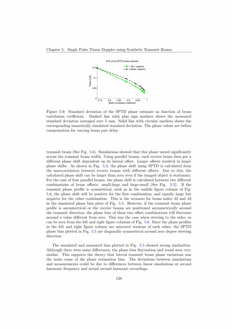
Chapter 5. Single Pulse Tissue Doppler using Synthetic Transmit Beams
0.75 0.8 0.85 0.9 0.95 10
0.05
0.1
0.15
Beam correlation coefficient
Pha
se [r
ad]
STD of the SPTD phase estimate
Sim. avg5mmMeas. avg5mm
Figure 5.9: Standard deviation of the SPTD phase estimate as function of beamcorrelation coefficient. Dashed line with plus sign markers shows the measuredstandard deviation averaged over 5 mm. Solid line with circular markers shows thecorresponding numerically simulated standard deviation. The phase values are beforecompensation for varying beam pair delay.
transmit beam (See Fig. 5.6). Simulations showed that this phase varied significantlyacross the transmit beam width. Using parallel beams, each receive beam then got adifferent phase shift dependent on its lateral offset. Larger offsets resulted in largerphase shifts. As shown in Fig. 5.2, the phase shift using SPTD is calculated fromthe autocorrelation between receive beams with different offsets. Due to this, thecalculated phase shift can be larger than zero even if the imaged object is stationary.For the case of four parallel beams, the phase shift is calculated between two differentcombinations of beam offsets: small-large and large-small (See Fig. 5.2). If thetransmit phase profile is symmetrical, such as in the middle figure column of Fig.5.6, the phase shift will be positive for the first combination, and equally large butnegative for the other combination. This is the scenario for beam index 42 and 43in the simulated phase bias plots of Fig. 5.5. However, if the transmit beam phaseprofile is asymmetrical or the receive beams are positioned asymmetrically aroundthe transmit direction, the phase bias of these two offset combinations will fluctuatearound a value different from zero. This was the case when steering to the sides, ascan be seen from the left and right figure columns of Fig. 5.6. Since the phase profilesin the left and right figure column are mirrored versions of each other, the SPTDphase bias plotted in Fig. 5.5 are diagonally symmetrical around zero degree steeringdirection.
The simulated and measured bias plotted in Fig. 5.5 showed strong similarities.Although there were some differences, the phase bias fluctuation and trend were verysimilar. This supports the theory that lateral transmit beam phase variations wasthe main cause of the phase estimation bias. The deviations between simulationsand measurements could be due to differences between linear simulations at secondharmonic frequency and actual second harmonic recordings.
129

5.5. Discussion
−5 0 5
0
20
40
60
80
100
120
Bmode image
Azimuth [mm]
Dep
th [m
m]
−10
−5
0
5
Vel
ocity
[cm
/s]
−10
−5
0
5
Vel
ocity
[cm
/s]
0 0.2 0.4 0.6 0.8−10
−5
0
5
Time [ms]
Vel
ocity
[cm
/s]
Figure 5.10: Comparison of velocity curves from the septum using SPTD and F2FTD.Narrow sector B-mode image with F2FTD sample volumes shown to the left. Thecorresponding velocity curves are shown to the right. The velocity curves from usingF2FTD are shown in solid blue line style and SPTD in dashed red line style.
5.5.2 Bias compensation
The bias compensation approach chosen in this work was to perform lateral averaging(See Fig. 5.8). This was possible since the bias has opposite polarity for beam pairswith positive and negative delay (see left plot in figure row two). Since the mechanismsof the bias were known, this averaging could be done in a way where only the minimumnumber of beams necessary to cancel out the bias were averaged. The main advantageof this approach is the robustness. It will work regardless of acquisition parametersand phase aberrations. It will also reduce the phase estimate variance due to averagingover a larger number of samples. An other approach could have been to pre-calculatethe bias based on models or simulations and subtract it. The advantage of such anapproach would be the higher lateral resolution of the velocity estimates. However, itis likely to fail due to aberrations. Fig. 5.7 shows that the bias changes significantlywith cardiac strength phase aberrations. This will make it impossible to accuratelypre-calculate the bias. Subtracting pre-calculated values might actually increase thebias in such scenarios. Another approach might be to estimate the phase bias fromrecorded data and then subtract it. Since the bias is depth varying, the bias wouldhave to be estimated for all depths. Such a method is beyond the scope of this work,but it is likely that it would be less robust than our proposed model based averaging.
For the two ranges investigated, 22.9 mm and 69.2 mm, the maximum absolutevelocity bias was reduced with 93.4% and 89.5% respectively. Since the beam pairdelay compensation scales the bias differently for positive and negative delay beam
130
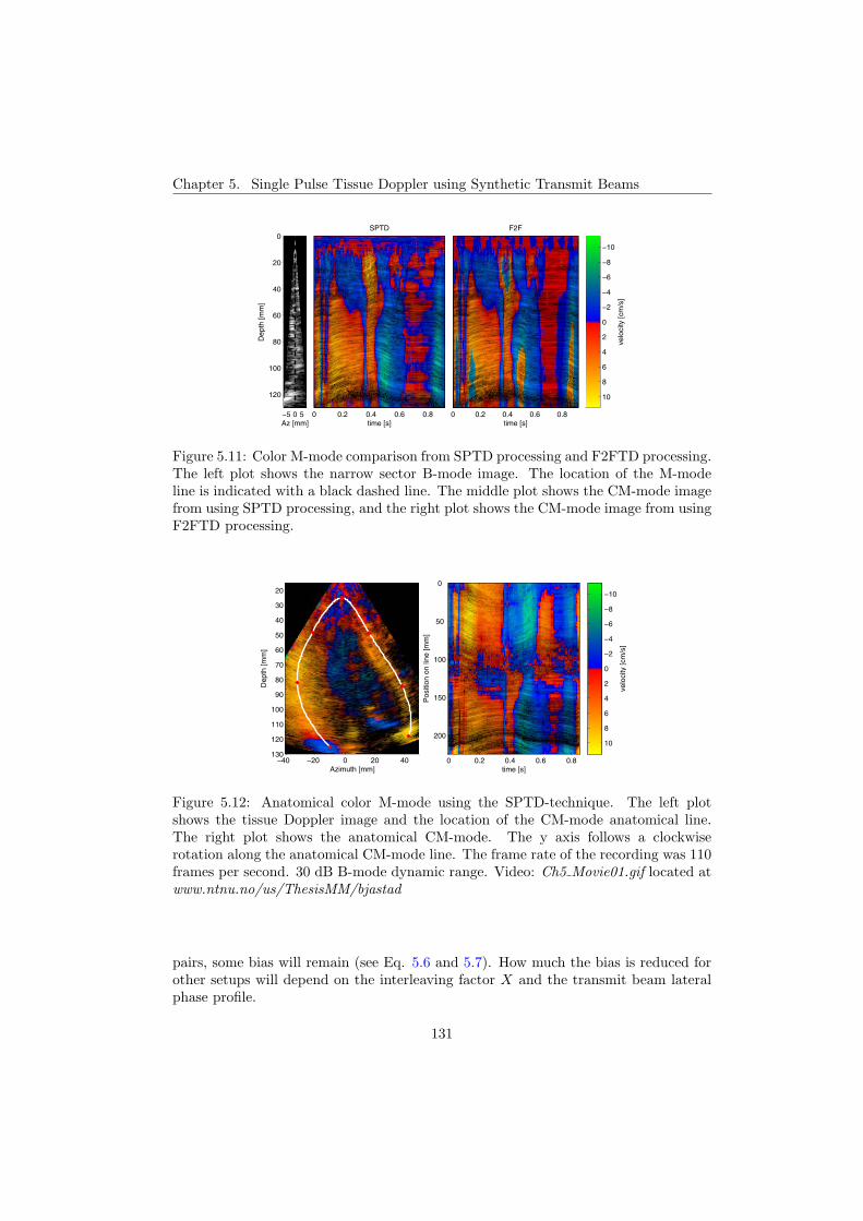
Chapter 5. Single Pulse Tissue Doppler using Synthetic Transmit Beams
−5 0 5
0
20
40
60
80
100
120
Az [mm]
Dep
th [m
m]
SPTD
time [s]0 0.2 0.4 0.6 0.8
F2F
time [s]0 0.2 0.4 0.6 0.8
velo
city
[cm
/s]
−10
−8
−6
−4
−2
0
2
4
6
8
10
Figure 5.11: Color M-mode comparison from SPTD processing and F2FTD processing.The left plot shows the narrow sector B-mode image. The location of the M-modeline is indicated with a black dashed line. The middle plot shows the CM-mode imagefrom using SPTD processing, and the right plot shows the CM-mode image from usingF2FTD processing.
Azimuth [mm]
Dep
th [m
m]
−40 −20 0 20 40
20
30
40
50
60
70
80
90
100
110
120
130
Pos
ition
on
line
[mm
]
time [s]0 0.2 0.4 0.6 0.8
0
50
100
150
200
velo
city
[cm
/s]
−10
−8
−6
−4
−2
0
2
4
6
8
10
Figure 5.12: Anatomical color M-mode using the SPTD-technique. The left plotshows the tissue Doppler image and the location of the CM-mode anatomical line.The right plot shows the anatomical CM-mode. The y axis follows a clockwiserotation along the anatomical CM-mode line. The frame rate of the recording was 110frames per second. 30 dB B-mode dynamic range. Video: Ch5 Movie01.gif located atwww.ntnu.no/us/ThesisMM/bjastad
pairs, some bias will remain (see Eq. 5.6 and 5.7). How much the bias is reduced forother setups will depend on the interleaving factor X and the transmit beam lateralphase profile.
131
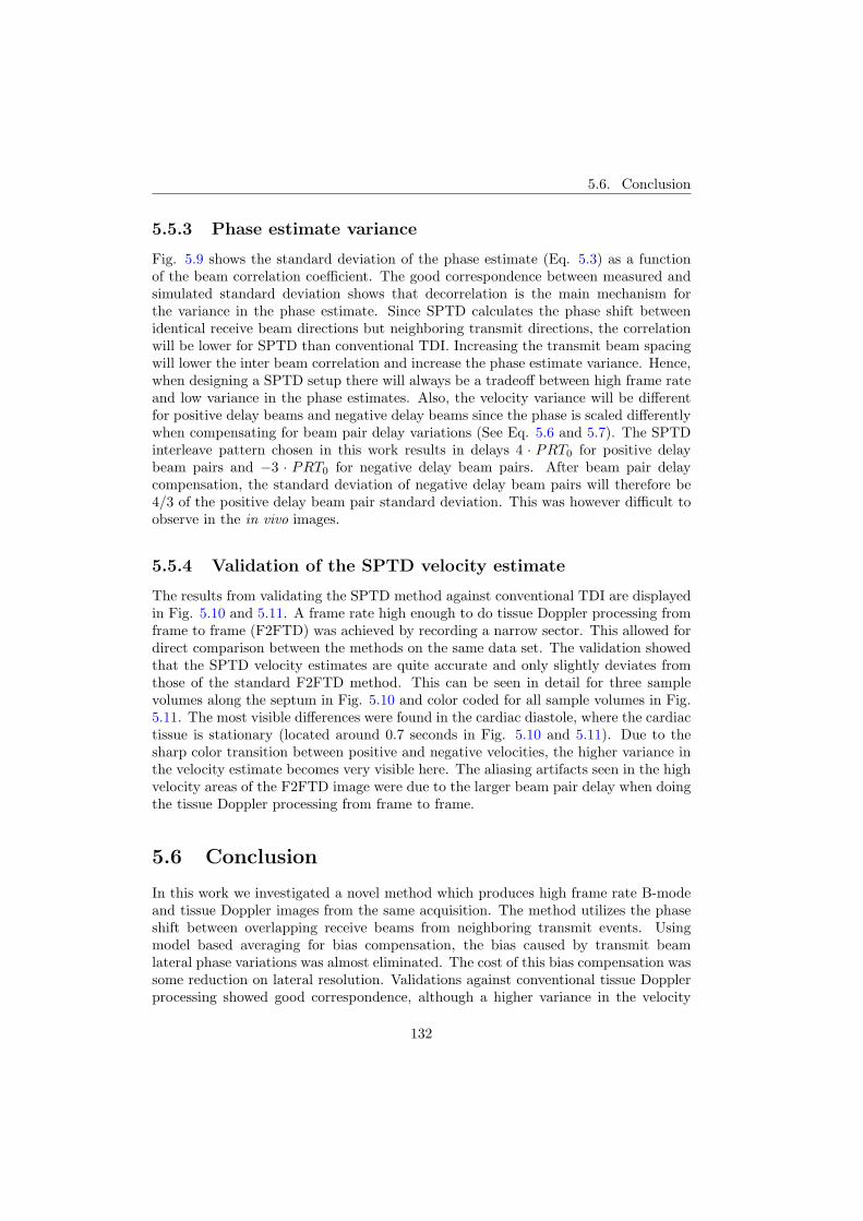
5.6. Conclusion
5.5.3 Phase estimate variance
Fig. 5.9 shows the standard deviation of the phase estimate (Eq. 5.3) as a functionof the beam correlation coefficient. The good correspondence between measured andsimulated standard deviation shows that decorrelation is the main mechanism forthe variance in the phase estimate. Since SPTD calculates the phase shift betweenidentical receive beam directions but neighboring transmit directions, the correlationwill be lower for SPTD than conventional TDI. Increasing the transmit beam spacingwill lower the inter beam correlation and increase the phase estimate variance. Hence,when designing a SPTD setup there will always be a tradeoff between high frame rateand low variance in the phase estimates. Also, the velocity variance will be differentfor positive delay beams and negative delay beams since the phase is scaled differentlywhen compensating for beam pair delay variations (See Eq. 5.6 and 5.7). The SPTDinterleave pattern chosen in this work results in delays 4 · PRT0 for positive delaybeam pairs and −3 · PRT0 for negative delay beam pairs. After beam pair delaycompensation, the standard deviation of negative delay beam pairs will therefore be4/3 of the positive delay beam pair standard deviation. This was however difficult toobserve in the in vivo images.
5.5.4 Validation of the SPTD velocity estimate
The results from validating the SPTD method against conventional TDI are displayedin Fig. 5.10 and 5.11. A frame rate high enough to do tissue Doppler processing fromframe to frame (F2FTD) was achieved by recording a narrow sector. This allowed fordirect comparison between the methods on the same data set. The validation showedthat the SPTD velocity estimates are quite accurate and only slightly deviates fromthose of the standard F2FTD method. This can be seen in detail for three samplevolumes along the septum in Fig. 5.10 and color coded for all sample volumes in Fig.5.11. The most visible differences were found in the cardiac diastole, where the cardiactissue is stationary (located around 0.7 seconds in Fig. 5.10 and 5.11). Due to thesharp color transition between positive and negative velocities, the higher variance inthe velocity estimate becomes very visible here. The aliasing artifacts seen in the highvelocity areas of the F2FTD image were due to the larger beam pair delay when doingthe tissue Doppler processing from frame to frame.
5.6 Conclusion
In this work we investigated a novel method which produces high frame rate B-modeand tissue Doppler images from the same acquisition. The method utilizes the phaseshift between overlapping receive beams from neighboring transmit events. Usingmodel based averaging for bias compensation, the bias caused by transmit beamlateral phase variations was almost eliminated. The cost of this bias compensation wassome reduction on lateral resolution. Validations against conventional tissue Dopplerprocessing showed good correspondence, although a higher variance in the velocity
132

Chapter 5. Single Pulse Tissue Doppler using Synthetic Transmit Beams
estimate. Using the SPTD technique, tissue Doppler images with a sector width of 65degrees were captured at a frame rate of 110 frames per second.
Acknowledgement
The researchers thank GE Vingmed Ultrasound for access to a Vivid 7 ultrasoundscanner.
133

5.6. Conclusion
134
References
[1] W. McDicken, G. Sutherland, C. Moran, and L. Gordon, “Colour doppler velocityimaging of the myocardium,” Ultrasound Med Biol, 1992.
[2] B. Lind, J. Nowak, J. Dorph, J. van der Linden, and L. A. Brodin, “Analysisof temporal requirements for myocardial tissue velocity imaging,” Eur JEchocardiogr, vol. 3, pp. 214–9, Sep 2002.
[3] H. Kanai, H. Hasegawa, N. Chubachi, Y. Koiwa, and M. Tanaka, “Non-invasiveevaluation of local myocardial thickening and its color-coded imaging,” IEEETransactions on Ultrasonics Ferro-electrics and Frequency Control, 1997.
[4] H. Kanai, M. Sato, Y. Koiwa, and N. Chubachi, “Transcutaneous measurementand spectrum analysis of heart wall vibrations,” IEEE Trans UFFC, 1996.
[5] C.-M. Yu, E. Chau, J. E. Sanderson, K. Fan, M.-O. Tang, W.-H. Fung,H. Lin, S.-L. Kong, Y.-M. Lam, M. R. Hill, and C.-P. Lau, “Tissue dopplerechocardiographic evidence of reverse remodeling and improved synchronicity bysimultaneously delaying regional contraction after biventricular pacing therapy inheart failure,” Circulation, 2002.
[6] M. Penicka, J. Bartunek, B. D. Bruyne, M. Vanderheyden, M. Goethals, M. D.Zutter, P. Brugada, and P. Geelen, “Improvement of left ventricular functionafter cardiac resynchronization therapy is predicted by tissue doppler imagingechocardiography,” Circulation, 2004.
[7] D. P. Shattuck, M. D. Weinshenker, S. W. Smith, and O. T. von Ramm,“Explososcan: A parallel processing technique for high speed ultrasound imagingwith linear phased arrays,” J. Acoust, Soc. Amer., vol. 75, no. 4, pp. 1273–1282,1984.
[8] O. T. von Ramm, S. W. Smith, and H. G. Pavy, “High-speed ultrasoundvolumetric imaging system – part ii: Parallel processing and image display,”IEEE transactions on ultrasonics, ferroelectrics, and frequency control, vol. 38,March 1991.
[9] T. Bjastad, S. A. Aase, and H. Torp, “The impact of aberration on high framerate cardiac b-mode imaging,” IEEE transactions on ultrasonics, ferroelectrics,and frequency control, vol. 54, January 2007.
135
References
[10] T. Hergum, T. Bjastad, K. Kristoffersen, and H. Torp, “Parallel beamformingusing synthetic transmit beams,” IEEE transactions on ultrasonics, ferroelectrics,and frequency control, vol. 54, February 2007.
[11] J. Kirkhorn, S. Bjærum, B. Olstad, K. Kristoffersen, and H. Torp, “A newtechnique for improved spatial resolution in high frame rate color dopplerimaging,” Proceedings IEEE Ultrasonics Symposium, 2003.
[12] S. Bjaerum, H. Torp, and K. Kristoffersen, “High frame rate tissue dopplerimaging,” Proceedings IEEE Ultrasonics Symposium, 2001.
[13] P. R. Detmer, J. R. Jago, and X.-N. Li, “Method and apparatus for obtainingb-flow and b-mode data from multiline beams in an ultrasound imaging system.”U.S. Patent 6,589,177 B1, 2002.
[14] M. Bernard J. Savord, Andover, “Method and apparatus for increasing the framerate and resolution of a phased array imaging system.” U.S. patent 5.318.033,1992.
[15] B. S. Robinson, “Ultrasonic diagnostic imaging systems with blended multilinefor 2d and 3d applications.” U.S. Patent 6.482.157, Mar. 30 2001.
[16] R. Chesarek, “Ultrasound imaging system for relatively low-velocity blood flowat relatively high frame rates.” U.S. Patent 4,888,694, 1989.
[17] R. F. Wagner, S. W. Smith, J. M. Sandrik, and H. Lopez, “Statistics of specklein ultrasound b-scans,” IEEE transactions on ultrasonics, ferroelectrics, andfrequency control, 1983.
[18] J. A. Jensen and N. B. Svendsen, “Calculation of pressure fields fromarbitrarily shaped, apodized, and excited ultrasound transducers,” IEEE Trans.Ultrason.,Ferroelec., Freq. Contr., 1992.
[19] L. M. Hinkelman, T. L. Szabo, and R. C. Waag, “Measurements of ultrasonicpulse distortion produced by human chest wall,” J. Acoust. Soc. Am., 1997.
[20] T. Johansen, B. Angelsen, and W. Nordhøy, “Phase aberrations - experimentsand simulations,” Proceedings of the 23rd Scandinavian Symposium on PhysicalAcoustics, 2000.
136