high dimensional sparse covariance estimation: accurate

Submitted to the Annals of Applied Probability

HIGH DIMENSIONAL SPARSE COVARIANCE ESTIMATION:ACCURATE THRESHOLDS FOR THE MAXIMAL DIAGONAL ENTRY

AND FOR THE LARGEST CORRELATION COEFFICIENT

By Aharon Birnbaum∗ and Boaz Nadler†

The Hebrew University∗ and Weizmann Institute of Science†

The maxima of many independent, or weakly dependent, randomvariables, and their corresponding thresholds for given right tail prob-abilities are classical and well studied problems. In this paper we focuson two specific cases of interest related to estimation and hypothe-sis testing of high dimensional sparse covariance matrices. These arethe distribution of the maximal diagonal entry of a sample covariancematrix and the largest off-diagonal correlation coefficient, both underthe assumption of an identity population covariance. In both cases, assample size and dimension tend to infinity, upon centering and scal-ing, there is asymptotic convergence to a Gumbel distribution. Weshow, however, that this convergence is slow and that finite sampledistributions may be quite far from these asymptotic ones. Applyinga perturbation approach, we identify the leading error terms, andderive more accurate distributions and corresponding thresholds. Fornon-Gaussian data, these depend explicitly on higher order momentsvia appropriate Edgeworth expansions. As a side result, we also de-rive sharp bounds for the left and right tail probabilities of a singleχ2

n random variable, which may be of independent interest.

1. Introduction. Many contemporary applications require analysis of high dimensionaldata, often with a relatively small number of samples, see [15] for a recent review. Prototyp-ical examples include hypothesis testing, inference on, and estimation of a p × p populationcovariance matrix Σ, or of its leading eigenvectors, given a sample covariance matrix S com-puted from only n samples [4, 17]. Another example is screening for pairs of highly correlatedvariables, see [11]. In the high-dimension small-sample setting (known as the “large p, smalln” scenario), considerable work has been devoted to various models of sparsity, to the develop-ment of thresholding schemes, and derivation of corresponding minimax rates of convergence,see for example [1, 5, 8, 18, 20, 25] and references therein. There are also works on estimationof a sparse inverse covariance matrix, though we shall not consider those in the present paper.

Assuming sparsity of either the population covariance matrix or of its leading eigenvectors,the two main thresholding schemes that have been proposed are: i) variable selection bythresholding the diagonal of the sample covariance matrix, and ii) screening highly dependentpairs of variables by thresholding the off-diagonal entries of sample covariance or correlationmatrices. Similar schemes have been suggested for various hypothesis testing problems andfor detection of sparse signals in noise.

On the theoretical front, for sparse covariance estimation, assuming that the underlyingdistribution satisfies appropriate tail conditions, several of the works cited above suggestedthresholds of the form C

√(ln p)/n. Using relatively crude tail bounds, it can be proved that

under various sparsity models such thresholds attain asymptotic consistency and in certain

AMS 2000 subject classifications: Primary 60F05; secondary 62E17

1

http://www.imstat.org/aap/

2 BIRNBAUM AND NADLER

cases even achieve the minimax rates as n, p → ∞. With respect to the largest off-diagonalentry of a sample correlation matrix, several works studied its limiting distribution as p, n →∞, assuming independence of all p coordinates, with an identity population covariance matrix,see [13, 6, 23, 35]. Beyond their theoretical interest, these results can be used to identify highlycorrelated pairs in high dimensional data and to reject hypotheses of variable independence.Indeed, such thresholding schemes have been proposed for detection of sparse signals in severalpractical applications. For example, Noh and Solo [28] proposed a thresholding scheme todetect signals in fMRI data, while Johnson and Potter [14] use a similar approach for outlierdetection in a passive microwave sensing application. For a discussion of the importance ofaccurate thresholds in fMRI studies, see for example [24].

Given the above asymptotic results, an interesting practical question is their accuracy andrelevance for typical applications, where the dimension and sample size are of course finite,with the latter parameter potentially rather small (n = O(10 − 100), with p = O(n) oreven p � n). In this paper we focus on the hypothesis testing aspect of these problems:the determination of accurate thresholds for given false alarm rates, and in particular theirdependence on the finite sample size and dimension, as well as on the underlying distributions.To set the corresponding thresholds for detection of sparse structures in data, we consider thenull hypothesis that the observed data Xi = (Xi1, . . . , Xip) contains no structure at all, with allits p coordinates being independent and having the same distribution. Under this assumption,the diagonal entries of the sample covariance matrix S are all i.i.d. random variables. Similarly,the off-diagonal entries of the correlation matrix R are also all identically distributed, thoughthey are weakly dependent. Hence, determination of appropriate thresholds for given type-I error probabilities amounts to the study of the maxima of many independent, or weaklydependent, random variables.

As is well known in extreme value theory, the convergence of the maxima to the limit-ing distribution may be very slow. In this paper we show that this is also the case for ourtwo random variables of interest, the maxima of the diagonal of S and the largest pairwisecorrelation coefficient, albeit in a non-trivial way. The main difference between the classicaltheory of extreme values [19] and our setting, is that in the former the distribution of the prandom variables is fixed and p → ∞, whereas our setting involves two parameters p and nwith the distribution of the underlying variables depending on the sample size n. To study themaxima of p such random variables, thus requires a careful analysis of various terms involvingboth of these parameters. In particular, we first point out that in the “large p – small n” set-ting, the standard approach of analyzing the relevant distributions in the joint limit as bothp, n → ∞ may give quite inaccurate results. The reason is that the leading asymptotic errorterms, as both p, n → ∞, typically of order O(ln ln p/ ln p), are not the leading cause of errorfor finite and small values of n. The key point of our analysis, is that in the non-asymptotic“large p– small n” setting, the main source of inaccuracy of the limiting extreme value dis-tributions is in different terms, of order O((ln p)3/2/

√n) or O((ln p)2/n), depending on the

variable of interest. Since these terms are asymptotically negligible compared to ln ln p/ ln p,by studying the asymptotic limit p, n → ∞ with dimension growing at most polynomiallywith sample size, these error terms are not considered, even though in practice they can beO(1). By explicitly taking these higher order terms into account, we derive modified distri-butions and corresponding thresholds, which are far more accurate for practical sample sizeand dimensionality.

In our analysis, we consider both Gaussian and non-Gaussian distributions. In the Gaussian

VARIANCE AND CORRELATION THRESHOLDS 3

case, we perform a delicate analysis of the known χ2 distribution for the diagonal of thecovariance matrix and of the distribution of Pearson’s correlation coefficient for independentbi-variate Gaussians. In the course of this analysis we also derive sharp bounds for the leftand right tail probabilities of a χ2

n random variable, which may be of independent interest.In the Gaussian case, we identify the correction terms as the leading order terms in the

Edgeworth expansion of these distributions. Hence, in the non-Gaussian case, we study thecorresponding Edgeworth expansions of the relevant distributions. The resulting modifiedthresholds thus depend explicitly on the higher order moments of the underlying distributions,and highlight the importance of Edgeworth expansions in high dimensional settings.

From a statistical perspective, our results allow determination of quite accurate non-asymptotic thresholds for a variety of hypothesis testing problems, as outlined above. In thecontext of high dimensional sparse linear regression [9], they allow to set appropriate thresh-olds for screening which predictor variables are highly correlated with a response variable.

However, our approach may have a broader applicability, as similar settings involving twoparameters n, p with p � 1, occur frequently in many other high dimensional problems. In thecontext of tail inequalities for the maxima of p variables, it is known that behavior may changefrom double exponential to exponential, see for example [34]. In cases where accurate distri-butional results are needed, our perturbation technique, considering the leading order termsas a function of the finite values of both p and n may thus be applicable. A notable exampleis detection of significant bi-clusters or ANOVA-fit submatrices in high dimensional rectan-gular matrices [33]. Our analysis has also implications to estimation of sparse eigenvectors inprincipal component analysis [5], but these will be discussed in a separate publication.

The paper is organized as follows. In section 2 we present the problem formulation, a reviewof previous work and our main results. The outline of the proofs appears in sections 3 and4, with more technical details postponed to the appendix. Section 5 contains simulationsillustrating the accuracy of our modified distributions and thresholds.

2. Problem Setup and Main Results. For i = 1, . . . , n+1, let Xi = (Xi1, Xi2, . . . , Xip)T ,be (n+1) i.i.d. p-dimensional column vectors, with an unknown population covariance matrixΣ. The (unbiased) p × p sample covariance matrix S is given by

(1) S =1n

n+1∑

i=1

(xi − x̄)(xi − x̄)T

where x̄ is the sample mean, whereas the (i, j)-th entry of the sample correlation matrix R is

(2) Rij =Sij√SiiSjj

.

As mentioned in the introduction, in several modern applications, thresholding the matricesS or R are common tasks for covariance estimation, detection of sparse structures and fortesting hypotheses of variable independence. The focus in this paper is on the determinationof non-asymptotic accurate thresholds for these tasks for given false alarm probabilities, whichdepend both on the finite sample size n and dimension p, and on the underlying distribution.

Given the assumption that the structure to be discovered is sparse, in our analysis of thecorresponding thresholds we consider the “null hypothesis” of no structure, i.e., we assumethat all Xij are i.i.d. from some underlying distribution p(x) with a sufficient number of finite


moments. Without loss of generality, we assume that E[Xij ] = 0, and E[X2ij ] = 1, so the

population covariance matrix is the identity matrix, Σ = I. For future use, we denote thehigher order moments by μk = E[Xk

ij ].

2.1. Diagonal Thresholding. Let us first consider the maxima of the diagonal entries ofthe sample covariance matrix, which we denote by Ynp,

(3) Ynp = max1≤i≤p

Sii.

Under the null hypothesis of no structure in the data, the diagonal entries Sii are all indepen-dent. Furthermore, as n → ∞ and under suitable moment conditions on p(x), from the CLT,each Sii converges in distribution to a Gaussian random variable. Due to the independenceof all Sii, the theory of extreme values then states that as p → ∞ the maxima, after propercentering and scaling, converges to a Gumbel distribution [19]. When the underlying dataXi are multivariate Gaussian N(0, 1), each Sii follows a χ2

n/n distribution. Approximatingeach diagonal entry by a N(1, 2/n) random variable, standard results on the maxima of pindependent Gaussians imply that the threshold z(p, α) which satisfies

(4) Pr

[

Ynp > 1 +

√2n

z(p, α)

]

= α

is asymptotically given by

(5) z2(p, α) = 2 ln p − ln ln p − ln 4π − 2 ln | ln(1 − α)| + O

(ln ln p

ln p

)

.

As can be verified numerically, Eqs. (4) and (5) are quite accurate for the maxima of p � 1i.i.d. Gaussian r.v.’s. The key difference in our setting is that the distribution of each of thep r.v. Sii is only approximately Gaussian and depends on a second parameter n. Due to theslow convergence of the χ2

n/n distribution to a N(1, 2/n) Gaussian distribution, Eq. (5) may

thus be a poor approximation to the required threshold. That is, the scaling√

2nz(p, α) in

Eq. (4) may not be sufficiently accurate, with the required threshold having a non-negligibledependence on n, z = z(n, p, α). To illustrate this point, and motivate our work, consider theplots in Fig. 1. In the three panels from left to right, we compare the empirical density ofYnp to the Gaussian threshold of Eq. (5), for (n, p) = (100, 1000), (1000, 500) and (1000, 100),respectively. Note that in the left panel with n � p, the distribution of Ynp is very far fromthe limiting Gumbel distribution corresponding to maxima of purely Gaussian r.v.’s. Even inthe other panels, where n = 2p or n = 10p, the fit is not very accurate.

Our first result elucidates on the reason for this discrepancy. We show that for a givenright tail probability α, the Gaussian approximation involves neglecting a higher order termO(z3/

√n) in the relevant equation for setting the threshold z(n, p, α). Since to leading order

z ∼ (ln p)1/2, asymptotically as p, n → ∞ with pn = c for example, this term not only vanishes

but is also significantly smaller than the next order correction term not present in Eq.(5), ofO(ln ln p/ ln p). However, for this term to be negligible for finite p, n, we need z3/2/

√n � 1.

Fig. 2(a) shows the slow decay of this term as n → ∞ with p = c ∙ n, for various values ofc. Even if n = 5p (c = 0.2), for this higher order term to be smaller than < 0.01, requires asample size n = O(106). This example illustrates that problems involving asymptotics with


1.4 1.5 1.6 1.7 1.8

0.02

0.04

0.06

0.08

0.1

0.12

Ynp

n = 100 p = 1000

sim. χ2n

Gauss tresh

χ2n tresh

1.1 1.13 1.16 1.19 1.22

0.02

0.04

0.06

0.08

0.1

Ynp

n = 1000 p = 500

sim. χ2n

Gauss tresh

χ2n tresh

1.05 1.1 1.15 1.2

0.02

0.04

0.06

0.08

0.1

Ynp

n = 1000 p = 100

sim. χ2n

Gauss tresh

χ2n tresh

Fig 1. Empirical density of Ynp (blue circles) compared to the asymptotic Gumbel distribution correspondingto the maxima of p Gaussians (solid red), and to our suggested correction, Eq. (6) (dashed black curve).

two or more small or large parameters (p, n in our case), need to be studied with extremecare. This is a well known issue in the applied mathematics literature, see [3].

Based on this observation, we suggest a modified threshold that takes this O(z3/√

n) terminto account. In the Gaussian case this modified threshold can be computed explicitly usingthe known distribution of a χ2

n random variable, as follows:

Theorem 2.1. Let {Sii}pi=1 be p i.i.d. random variables Sii ∼ χ2

n/n, and let Ynp denote

their maxima. Let t = 1 +√

2nzH , where zH = zH(n, p, α) is given by

(6) zH(n, p, α) = z(p, α)

(

1 +13

√2n

z(p, α)3

1 + z(p, α)2

)

and z(p, α) is the Gaussian threshold from Eq.(5). Then, for parameter values (n, p) such that

(ln p)3/2 �√

n � (ln p)5/2

ln ln p ,

(7) Pr [Ynp < t] = (1 − α)

(

1 + O

(ln(1 − α)

ln p

)

+ O

(| ln(1 − α)|2

p

))

.

As shown in Figure 1, the modified expression of Eq.(6) yields a much better fit to theempirical density of Ynp for several values of (n, p). In particular, the fit is very accurate inthe right tail, the most relevant region for calculation of the threshold zH . The broad rangeof values of (n, p) where Eq. (6) is the leading correction term is illustrated in Figure 2(b).

To clarify the origin of the correction term in Eq. (6) we describe the first steps in thecalculation of zH . Since Sii are i.i.d. we look for a threshold t = t(α) s.t.

Pr[Ynp < t] = (1 − Pr[S11 > t])p = 1 − α.

To this end, we should plug into this equation some expression for Pr[S11 > t]. Since S11 ∼χ2

n/n we use the following approximation (taken from lemma 3.1 below)

Pr[S11 > 1 + ε] ≈e−

n2 (ε−ln(1+ε))

√πn(ε + 2

n).


103

104

105

106

0

0.05

0.1

0.15

0.2

0.25

0.3

z(p,0.05)3/2√

n

n

c = 0.2c = 0.5c = 1c = 2c = 5c = 10

(a)

0 0.5 1 1.5 2

x 104

0

0.2

0.4

0.6

0.8

1

1.2

1.4

1.6

1.8

2x 10

4

p

n

Gaussian approximation valid

Finite sample correction





(ln p)5/(ln ln p)2

n = p

(ln p)3

(b)

Fig 2. (a) The ratio z(p,α)3/2√

nas a function of sample size n with α = 0.05 and p = c ∙n for various values of c.

(b) Following the conditions of Theorem 2.1, the top and bottom solid curves are (ln p)5/(ln ln p)2 and (ln p)3,respectively whereas the diagonal dashed curve is n = p. For sample size n significantly above the top curve(which in particular implies n � p for p ≤ 20000), the Gaussian approximation (Eq. (5)) is reasonably accuratewith all correction terms being negligible. Between the two curves finite n corrections are non-negligible. Belowthe bottom curve, p is exponential in n, and a different asymptotic approximation is needed.

Replacing ln(1 + ε) by its Taylor expansion, and making a change of variables ε =√

2nz gives

Pr[

S11 > 1 +√

2nz

]

≈e−z2/2

√2πz

∙e−

n2

∑∞k=3

(−√

2n

z)k/k)

1 +√

2n

1z

.(8)

Let us compare this expression with the tail behavior for a Gaussian r.v., whereby for z � 1

Pr [N(0, 1) > z] =e−z2/2

√2πz

(

1 + O

(1z

))

.

Thus approximating χ2nn by N(1, 2

n), implicitly implies replacing the second term in Eq.(8) byunity. In particular for this approximation to be accurate, the next order term must be small√

2nz(p, α)3 � 1. However, as discussed above (and illustrated in Fig. 2(a)), this term is in

fact O(1) for practical finite values of (n, p) which explains the poor accuracy of Eq. (5) as athreshold for the maxima of many χ2

n r.v.’s.In summary, even though as n → ∞ each diagonal entry Sii converges to a Gaussian distri-

bution, for finite values of n, p the Gaussian approximation may not be sufficiently accurateand a more careful analysis is required. When the observed data Xij ∼ N(0, 1), the leading

correction term follows from an explicit analysis of the tail of a χ2n

n r.v., and in fact involvesits Edgeworth expansion as n → ∞. In the general case, there is no explicit expression forthe distribution of the sample variance. In analogy to the χ2

n/n case, we propose a modifiedthreshold that takes into account the first term in the Edgeworth expansion of the samplevariance. This gives the following proposition:


Proposition 2.1. Let S be the sample covariance matrix of an (n + 1) × p matrix X,whose entries Xij are all i.i.d. from some density p(x) with zero mean, unit variance, and

finite 8-th moments. Further assume that lim sup‖t‖→∞

∣∣∣E[ei(t1X11+t2X2

11)]∣∣∣ < 1. Let

(9) zE(n, p, α) = z(p, α)

(

1 +κ

6σ3

1√

n

z(p, α)3

1 + z(p, α)2

)

where z(p, α) is the Gaussian threshold from Eq.(5), and

σ2 = μ4 − 1(10)

κ = μ6 − 3μ4 + 6μ23 + 2.(11)

Then, for parameter values (n, p) such that (ln p)3/2 �√

n � (ln p)5/2

ln ln p ,

(12) Pr[

Ynp < 1 +σ√

nzE(n, p, α)

]

≈ 1 − α.

Note that for a Gaussian distribution, σ2 = 2, κ = 8, and we recover Eq. (6) of Theorem2.1. Figure 3 compares the empirical density of Ynp for several underlying distributions, tothe limiting Gumbel density and to the density corresponding to Eq.(12). While our proposedthreshold Eq.(9) is more accurate than the Gaussian threshold, its accuracy varies for differentdistributions. In contrast to the Gaussian case where Eq. (7) contained explicit error bounds,the errors involved in Eq. (12) are related to the accuracy of Edgeworth expansions. Derivingsharp (non-uniform and location dependent) bounds on the error of Edgeworth expansions isan interesting research topic beyond the scope of this article.

2.2. Largest Correlation Coefficient. Next, we consider the largest correlation coefficient,namely the maximal off-diagonal entry, in absolute value, of the sample correlation matrix,

(13) Ln = maxi<j

|Rij |.

The random variable Ln was suggested as a statistic for testing independence of p variatesof a population, see [23, 26]. Related random variables, such as the maxima of individualrows of the correlation matrix R were recently suggested for screening interesting variables inlarge-scale correlation studies, see [11, 32]. Similarly, in the context of ultrahigh dimensionalregression, screening variables based on their correlation with a response was studied by Fanand Lv [9]. Finally, the distribution of Ln plays a role in compressed sensing, since Ln is thecoherence of the design matrix X, see [6].

The limiting distribution of Ln, in the joint limit n, p → ∞ has been studied in severalworks. In [13], Jiang showed that if n/p → γ ∈ (0,∞) and E[Xr] < ∞ for some r > 30, then

(14) nL2n − 4 ln p + ln ln p → exp

(−e−y/2/

√8π)

.

Since then, several works showed that Eq.(14) continues to hold both with weaker momentconditions, as well as when the dimension is allowed to increase polynomially with sample


1.15 1.2 1.25 1.3 1.35 1.4 1.45 1.50

0.02

0.04

0.06

0.08

0.1

0.12

Ynp

Uniform p = 200, n = 100

simulationGaussiannew

1.5 2 2.5 30

0.02

0.04

0.06

0.08

0.1

0.12

0.14

Ynp

exp p = 200, n = 100


1.4 1.6 1.8 2 2.2 2.4 2.6 2.8 30

0.02

0.04

0.06

0.08

0.1

0.12

0.14

0.16

0.18

0.2

Ynp

t7 p = 200, n = 100


1.4 1.6 1.8 2 2.2 2.4 2.6 2.8 30

0.05

0.1

0.15

0.2

0.25

Ynp

χ27 p = 200, n = 100


Fig 3. Comparison of the empirical density of Ynp (blue circles) to the asymptotic Gumbel density of themaxima of p i.i.d. Gaussians, Eq. (5) (solid red), and to our suggested correction, Eq. (6) (dashed black curve).

size, see [6, 22] and additional references therein. When dimension increases exponentiallywith sample size, there is a phase transition in the limiting distribution, see [7].

As in the case of the maxima of the diagonal entries of S, a key question is the accuracyof Eq.(14) for finite p, n, and in particular when n � p. Moreover, the parameter p has adifferent role here, as we now consider the maxima of p(p − 1)/2 weakly dependent randomvariables, instead of only p variables as in the previous section. That is, even a modest valueof p leads to the maxima of many random variables. In general, as already mentioned above,the convergence to limiting extreme value distributions is known to be slow. Indeed, in [23],the authors showed that the convergence rate in Eq. (14) is very slow, of O(ln ln n/ ln n).Then, assuming that p, n → ∞ with c1n

β < p < c2nβ for some β > 0, and assuming

some appropriate regularity conditions on the underlying distribution, Liu et. al. derivedthe following improved approximation (Thm. 1.2 in [23]), with a universal correction termindependent of the underlying distribution,

(15) Pr[nL2

n − 4 ln p + ln ln p < y]≈ exp

(

−p(p − 1)

2Pr[χ2

1 > 4 ln p − ln ln p + y])

.


-5 0 50

0.05

0.1

0.15

0.2

p = 64, N = 256

U

simGumbelLLSTheory

2 4 6 80

0.005

0.01

0.015

0.02

0.025

0.03

0.035p = 64, N = 256

U

simGumbelLLSTheory

-5 0 50

0.05

0.1

0.15

0.2

0.25p = 256, N = 64

U

simGumbelLLSTheory

Fig 4. Empirical density of U = nL2n − 4 ln p + ln ln p (blue circles) in comparison to the asymptotic Gumbel

density, Eq. (14), (solid red curve), the correction by Liu, Lin and Shao (LLS) [23], Eq. (15), (dashed-dotblack), and to our suggested correction, Eq. (17) (dashed purple curve). The left panel is for (p, n) = (64, 256),the center panel is a zoom into the right tail region, whereas the right panel is for (p, n) = (256, 64).

Liu et. al. further showed that asymptotically, Eq. (15) has a smaller error, O((ln n)5/2/

√n).

In this paper we are interested in accurate approximations to the right tail probabilities ofLn. To motivate our work, consider the plots in Figure 4, which compare the empirical densityof nL2

n −4 ln p+ln ln p to the limiting distribution (14) and to its correction (15) as suggestedby [23], both for (n, p) = (256, 64) as well as for (n, p) = (64, 256), with underlying N(0, 1)observations. As seen from these plots, neither (14) nor (15) provide accurate approximationsto the required distributions, even though the latter is slightly better.

As we show below, and similar to the analysis of the random variable Ynp, the source for thisnon-negligible error is in a term of asymptotically smaller order O((ln p)2/n), which was notconsidered in these previous works. In the Gaussian case, this term can be computed explicitly,using the known distribution of a single Pearson’s correlation coefficient for independent bi-variate Gaussian observations. Taking this term into account yields the following result:

Theorem 2.2. Let R be the correlation matrix of an (n + 1)× p matrix X, whose entriesXij are all i.i.d. N(0, 1). Let

(16) w(y) = 2 ln(p(p − 1)) − ln ln(p(p − 1)) + ln 2 + y.

Then, as p, n → ∞, with p/n → c(17)

Pr[

L2n <

w(y)n − 2

]

= exp

(

−e−y/2

√8π

∙ A(w(y), n, p)

)[

1 + O

(1n

,1

√n(ln p)3/2

)

e−y/2]

+ O(e−y)

where

(18) A(w, n, p) = e−w2/4(n−2)(

1 −n − 2

n

1w

)√2 ln(p(p − 1))

w.

As illustrated in Fig. 4, Eq. (17) provides a much better fit to the empirical density of Ln

than the asymptotic Gumbel distribution of Eq. (14), in particular at the right tail, which isthe most relevant part for threshold calculation.


It is instructive to compare the difference between Eq. (17) and the limiting expression (14).Note that the latter follows from the former under the approximation A(w, n, p) ≈ 1. For thelimiting expression to be accurate, a necessary condition is thus that w2/4n � 1. Since forlarge p, to leading order w = 4 ln p(1 + o(1)), for this term to be negligible in practice, sayw2/4n = 0.1, the required condition is n ≥ 40(ln p)2. Even at a moderately small dimension ofp = 10, for the asymptotic distribution to be accurate requires n & 200 samples. Our analysisthus illustrates that even with Gaussian observations, for practical values of (n, p) the limitingformula (14) may be quite far from the empirical one for the largest correlation coefficient,and as far as testing is concerned, may lead to rather inaccurate thresholds.

Let us provide a different point of view on the expression A(w, n, p). As n → ∞, each indi-vidual correlation coefficient Rij converges in distribution to a Gaussian N(0, 1/

√n) random

variable. The term exp(−w2/4(n−2)) appearing in A(w, n, p) is nothing but the leading ordercorrection term in the Edgeworth expansion of the sample correlation coefficient, correspond-ing to independent bi-variate Gaussian observations. When the underlying random variablesXij are non-Gaussian, an explicit expression for the density of the sample correlation coeffi-cient is in general unknown. In analogy to the Gaussian case, we thus propose to approximatethe probability Pr[|Rij | > t] by its leading Edgeworth expansion.

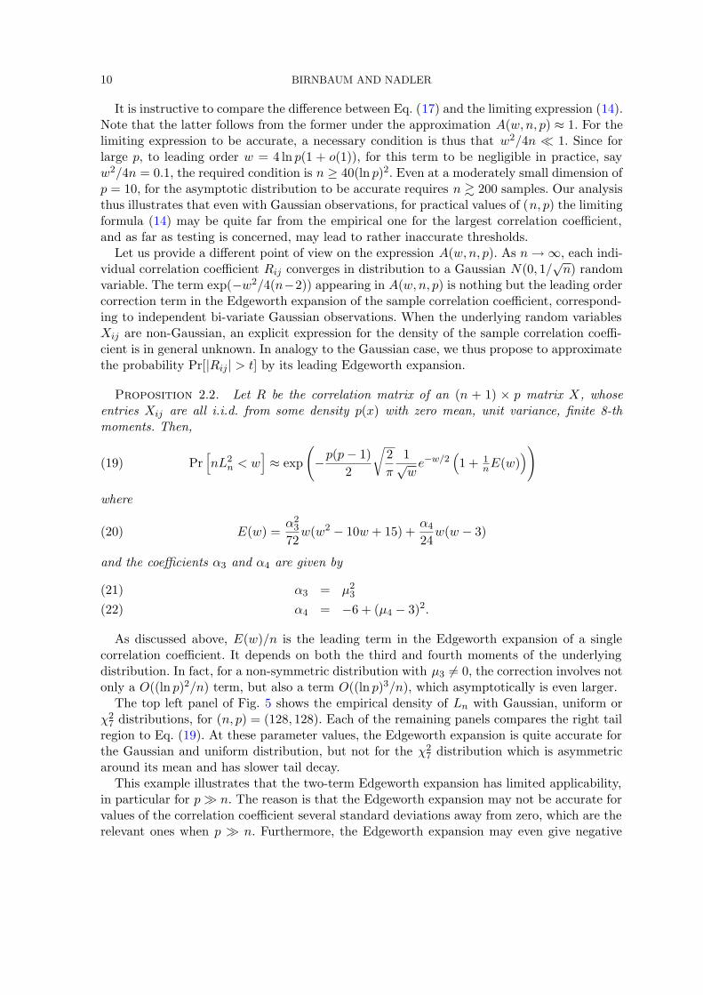
Proposition 2.2. Let R be the correlation matrix of an (n + 1) × p matrix X, whoseentries Xij are all i.i.d. from some density p(x) with zero mean, unit variance, finite 8-thmoments. Then,

(19) Pr[nL2

n < w]≈ exp

(

−p(p − 1)

2

√2π

1√

we−w/2

(1 + 1

nE(w)))

where

(20) E(w) =α2

3

72w(w2 − 10w + 15) +

α4

24w(w − 3)

and the coefficients α3 and α4 are given by

α3 = μ23(21)

α4 = −6 + (μ4 − 3)2.(22)

As discussed above, E(w)/n is the leading term in the Edgeworth expansion of a singlecorrelation coefficient. It depends on both the third and fourth moments of the underlyingdistribution. In fact, for a non-symmetric distribution with μ3 6= 0, the correction involves notonly a O((ln p)2/n) term, but also a term O((ln p)3/n), which asymptotically is even larger.

The top left panel of Fig. 5 shows the empirical density of Ln with Gaussian, uniform orχ2

7 distributions, for (n, p) = (128, 128). Each of the remaining panels compares the right tailregion to Eq. (19). At these parameter values, the Edgeworth expansion is quite accurate forthe Gaussian and uniform distribution, but not for the χ2

7 distribution which is asymmetricaround its mean and has slower tail decay.

This example illustrates that the two-term Edgeworth expansion has limited applicability,in particular for p � n. The reason is that the Edgeworth expansion may not be accurate forvalues of the correlation coefficient several standard deviations away from zero, which are therelevant ones when p � n. Furthermore, the Edgeworth expansion may even give negative


densities for small sample sizes. While beyond the scope of this paper, one option to remedythis may be to apply some monotonic transformation that prevents negative densities withoutlosing the asymptotic accuracy of the Edgeworth expansion, see for example [30].

Finally, the following proposition provides approximate expressions for the threshold of thelargest correlation coefficient. Its proof, based on algebraic manipulations of Eqs. (17) and(19), is similar to that made in deriving the thresholds for the maximal diagonal entry of thesample variance, and is hence omitted.

Proposition 2.3. Let R be the correlation matrix of an (n + 1) × p matrix X, whoseentries Xij are all i.i.d. from some density p(x) with zero mean, unit variance, finite 8-thmoments. Let

(23) w(n, p, α) = w0(n, p, α)(1 + δ)

where

(24) w0(n, p, α) = 2 ln(p(p − 1)) − ln ln(p(p − 1)) − ln 4π − 2 ln | ln(1 − α)|

and

(25) δ =

− w20

2(n−2)

(1 + w0 + w2

0n−2

)−1Xij ∼ N(0, 1)

2E(w)n−1

(1 + w0 −

E(w)n−1

)−1otherwise

.

Then for parameter values (n, p) such that (ln p)2 � n � (ln p)3

ln ln p

(26) Pr[(n − 2)L2

n < w(n, p, α)]≈ 1 − α

For the case of Gaussian observations, similar to the analysis in Theorem 2.1, the error inEq. (26) can be bounded explicitly. This error is O(ln(1 − α) ln ln p

ln p ) + O(ln2(1 − α)).

3. Largest Diagonal Entry of the Sample Covariance Matrix. In this section weprove Theorem 2.1 and Proposition 2.1. Recall that under the null hypothesis of no structurethe variables Xij are assumed to be all i.i.d. Hence their sample variances Sii are also i.i.d.and the exact equation for the threshold t as a function of the false alarm rate α is

(27) 1 − α = Pr[Ynp < t] = (1 − Pr[S11 > t])p .

To simplify notation we denote At = Pr[S11 > t]. Note that in fact At depends also on n sincethe distribution of Sii depends on n. Taking logarithms on both sides of Eq. (27) gives

(28) ln(1 − α) = p ln(1 − At).

Since our interest is in right tail probabilities of the maxima Ynp where p is also large, we mayassume that At � 1 and use the Taylor approximation ln(1 − At) = At + O(A2

t ). Thus,

(29) ln(1 − α) = −p(At + O(A2t )) ≈ −pAt.

An approximate threshold t = t(α) can be found by inverting Eq.(29), namely t(α) =A−1(ln(1 − α)1

p). The proof proceeds as follows: First we derive an explicit expression forAt as function of n and t. Next, we plug this expression into Eq. (29) and solve for t, care-fully analyzing the different error terms for finite p, n. We finish with an analysis of the errorincurred by the approximations performed in the various steps of the derivation.


0 2 4 6 80

0.01

0.02

0.03

0.04

0.05

0.06

U

p = 128, N = 128

N(0,1)U

χ27

Gumbel

0 2 4 6 80

0.01

0.02

0.03

0.04

0.05

0.06Gaussian

U

simGumbelGaussEW

0 2 4 6 80

0.01

0.02

0.03

0.04

0.05

0.06Uniform

U

simGumbelEW

0 2 4 6 80

0.01

0.02

0.03

0.04

0.05

0.06χ2

7

U

simGumbelEW

Fig 5. Empirical density of U = nL2n − 4 ln p + ln ln p for various underlying distributions (Gaussian, uniform,

and χ27), and comparison to the corresponding Edgeworth expansion (EW).

3.1. Gaussian case. In the multivariate Gaussian case, where Xi = (Xi1, . . . , Xip)T ∼N(0, Ip), each Sii follows a χ2

n/n distribution. The following lemma gives non asymptoticbounds for the left and right tails of the χ2

n distribution. This lemma may be of independentinterest, as χ2

n random variables appear in many statistical applications. In our case it providesan approximate yet accurate explicit expression for At = Pr[S11 > t].

Lemma 3.1. Let Wn be a random variable with a χ2n distribution. The following bounds

hold for all n ≥ 2 and for all ε > 0,

Pr[Wn

n> 1 + ε

]

≤1

√πn

1

ε + 2n

exp(−n

2 (ε − ln(1 + ε)))

(30)

Pr[Wn

n< 1 − ε

]

≤1

√πn

1 − e−n2 (ε− 2

n)

ε − 2n

exp(

n2 (ε + ln(1 − ε))

)(31)

In addition, if ε ≥√

2nz for some z > 1 then the following lower bound also holds

Pr[Wn

n> 1 + ε

]

≥1

√πn

1

ε + 2n

exp(−n

2 (ε − ln(1 + ε)))(

1 −1z2

−1n

)

.(32)

Remark 1: For ε < 2n it might seem that Eq. (31) gives a negative bound. However, this is

not the case since the numerator and the denominator in the term 1−e−n

2 (ε− 2n)

ε− 2n

have equal


sign for all ε. Additionally, there is no singularity at ε = 2n since as ε → 2

n both the numeratorand the denominator vanish and the limit is well defined.Remark 2: Several works derived χ2

n bounds via various approximations to the exponentialterms exp(−n

2 (ε− ln(1+ ε)) and exp(

n2 (ε + ln(1 − ε))

). For example, [17] and [21] proved that

Pr[Wn

n> 1 + ε

]

≤ exp(−n

4 (√

1 + 2ε − 1)2)

(33)

Pr[Wn

n< 1 − ε

]

≤ exp

(

−nε2

4

)

.(34)

Such bounds were mostly used to analyze minimax rates or prove consistency results. Theyare not sharp enough to determine accurate thresholds, which is the goal of this paper.Remark 3: Lemma 3.1 slightly improves on the results in [16] as follows. Let ε = s

√2/n,

and σn =√

2n. For 0 < s <√

n8 combining Eq. (47) of [16],

ln(1 + ε) − ε ≤−ε2/2

1 + 2ε/30 ≤ ε ≤

12

with our Eq. (30) gives that

(35) Pr [Wn − n > sσn] ≤1

√2π

1

s +√

2n

exp

(

−s2/2

1 + 4s/3σn

)

which is slightly sharper than Eq. (43) in [16] as it has a smaller pre-exponential factor.Furthermore, from Eq.(35) it follows that Eq. (44) in [16], namely that for 0 < s < n1/6

(36) Pr [Wn − n > sσn] ≤1se−s2/2

holds for any n ≥ 2, and not only for n ≥ 16, as stated in [16].We now return to our goal of deriving an explicit expression for the threshold t. We note

that Eq.(30) and (32) imply that as n → ∞ with t = 1 + ε, and ε =√

2nz with z ≥ z0 > 1,

(37) At = Pr[Wn

n> 1 + ε

]

=exp

(−n

2 (ε − ln(1 + ε)))

√πn(ε + 2

n)

(

1 + O

(1z20

,1n

))

.

Plugging Eq.(37) into Eq.(29) gives

(38) − pexp

(−n

2 (ε − ln(1 + ε)))

√πn(ε + 2

n)

(

1 + O

(1z20

,1n

))

= ln(1 − α).

As described in section A.2 of the appendix, algebraic manipulations of Eq.(38) yield the

following equation for z =√

n2 ε

(39) z2 −23

√2n

z3 + ln z2 + O

(z4

n,

1√

nz,

1z20

,1n

)

= 2 ln p − ln 2π − 2 ln | ln(1 − α)|.

Eq. (39) is an approximate transcendental equation for the required z. We look for the asymp-totic solution for z(α, p, n), under the assumption that n, p � 1. It is common in extreme valuetheory to take only the first three terms in an asymptotic expansion. These are given by:


Lemma 3.2. As p, n → ∞, with (ln p)3/2 �√

n, the first three terms in the asymptoticsolution of Eq. (39) are

(40) z2χ(α, p) = 2 ln p − ln ln p − ln 4π − 2 ln | ln(1 − α)| + o(1)

Remark: Note that the condition (ln p)3/2 �√

n holds for p = O(n) as well as for p = O(nβ)for any finite β > 0. However the condition does not hold if p = O(enc).

Lemma 3.2 shows that the first terms in the asymptotic expansion for the threshold z forthe χ2

n case are identical to those of Eq.(5), which corresponds to the Gaussian case. As shownin Figure 1 this might be quite inaccurate for finite values of p, n which hints that the o(1)terms in Eq. (40) may be non-negligible. To elucidate the source of this inaccuracy we plugthe value of zχ back into the original equation (39) and obtain that the residual is:

(41)23

√2n

z3χ + O

(1z20

,1n

)

.

Note that for a fixed 0 < α < 1 (and bounded away from 1), as p → ∞, zχ ∼√

2 ln p and z0 =√

ln p. Therefore, the assumption√

n � (ln p)5/2

ln ln p implies that z3√

n= O

((ln p)3/2

√n

)� O

(1

ln p , 1n

).

Hence the first term in Eq. (41) is the leading residual error. Moreover, it is significantly larger

than the errors incurred in the derivation of Eq.(39). Additionally, while (ln p)3/2√

nis negligible

in the limit n, p → ∞ its convergence to zero is very slow. As shown in Figure 2(a), for the

condition (ln p)3/2√

n< 0.1 to hold requires n ≥ 105 for a wide range of values of p/n. Hence we

should not neglect this term for practical finite values of n, p.To derive a more accurate threshold for finite values of n and p we return once more to

Eq. (39). This time, we view the term 23

√2nz3 as a perturbation and look for a solution of the

form z = zχ(1 + γ) where zχ is the asymptotic solution from Eq. (40) and γ = γ(n, p) = o(1).Plugging this expansion into Eq. (39) gives the following leading order equation for γ

2γz2χ + 2 ln(1 + γ) −

23

√2n

z3χ + ln

(1 − ln ln p+ln 4π+2 ln | ln(1−α)|

2 ln p

)= 0.

Since γ = o(1) we approximate ln(1 + γ) = γ + O(γ2) to get

2γ(1 + z2χ) =

23

√2n

z3χ − ln

(1 − ln ln p+ln 4π+2 ln | ln(1−α)|

2 ln p

)

The first term in the r.h.s. is of order O(

(ln p)3/2√

n

)while the second term is O

(ln ln pln p

). Hence,

if√

n � ln(p)5/2

ln ln p , the leading term in the r.h.s. is the first one and the leading solution for γ is

(42) γ =13

√2n

z3χ

1 + z2χ

.

This value of γ gives the threshold zH of Eq. (6). If we plug zH back into Eq.(39) we get that

the leading error term is now O(

1z20

)= O

(1

(ln p)2

)which also appears in the original equation.


To finish the proof of Theorem 2.1 we analyze the errors incurred by using the thresholdzH . This analysis is done by going ”backward” in the derivation of zH and collecting the error

terms in the various steps. Since εH =√

2nzH is the solution of Eq.(38) and zH >

√ln p,

(43) − pexp

(−n

2 (εH − ln(1 + εH)))

√πn(εH + 2

n)

(

1 + O

(1

ln p,1n

))

= ln(1 − α).

Recall that by our assumption ln p � n. Thus, the error term in the last equation is O( 1ln p).

By Eq.(37) we have that

(44) AtH

(

1 + O

(1

ln p

))

=exp

(−n

2 (εH − ln(1 + εH)))

√πn(εH + 2

n).

Thus from the last two equations we have that

(45) − pAtH = ln(1 − α)(

1 + O

(1

ln p

))

We use once more the Taylor approximation p ln(1 − AtH ) = −pAtH + O(pA2tH

) to get

(46) p ln(1 − AtH ) = ln(1 − α)(

1 + O

(1

ln p

))

+ O(pA2tH

).

Exponentiating this equation and approximating ex = 1 + x + O(x2) gives

Pr

[

Ynp < 1 +

√2n

zH

]

= (1 − AtH )p = (1 − α)(

1 + O

(ln(1 − α)

ln p

)

+ O(pA2tH

))

Using the approximation pA ≈ | ln(1 − α)| (see Eq. (45)) gives Eq. (7).�

3.2. Non-Gaussian case. To prove Proposition 2.1, which considers non-Gaussian obser-vations, we first derive an explicit approximate expression for Pr[Sii > t], that depends onthe higher order moments of the underlying distribution p(x) of the observations.

Lemma 3.3. Let X1, . . . , Xn+1 be n + 1 i.i.d. scalar random variables with some den-sity p(x) that has zero mean, unit variance, and finite 8-th moments. Further assume that

lim sup‖t‖→∞

∣∣∣E[ei(t1X11+t2X2

11)]∣∣∣ < 1. Then, as n → ∞, the Edgeworth expansion of the dis-

tribution of the unbiased sample variance estimator S = 1n

∑(xi − x̄)2 is

(47) Pr[

S > 1 +σ√

nz

]

= 1 − Φ(z) +φ(z)√

n

κ

6σ3(z2 − 1) + O

(1n

)

where Φ(z) is the c.d.f. of a N(0, 1) Gaussian r.v., φ(z) = e−z2/2√

2πis its density, and

σ2 = μ4 − 1(48)

κ = μ6 − 3μ4 + 6μ23 + 2.(49)


Lemma 3.3 is proven in appendix A.4. Plugging Eq.(47) into Eq.(29) and approximatingΦ(z) ≈ 1 − φ(z)

z yields the following approximate equation for the threshold z(n, p, α)

(50) − pe−z2/2

√2πz

(

1 +κ

6σ3

z√

n(z2 − 1)

)

= ln(1 − α).

Taking logarithms and approximating ln(1 + cz(z2 − 1)) ≈ cz3 gives the following equation:

(51) z2 −κ

6σ3

2√

nz3 + ln z2 = 2 ln p − ln 2π − 2 ln | ln(1 − α)|.

The only difference between Eq. (51) and Eq.(39) for the Gaussian case, is in the coefficientof the z3

√n

term. Solving Eq. (51) in the same way as we solved Eq. (39) gives Eq. (9).

4. Largest Correlation Coefficient. In this section we prove Theorem 2.2 and Propo-sition 2.2, regarding the distribution of the largest off-diagonal correlation coefficient. Thefirst step is to derive an approximate relation between Pr[maxi<j |Rij | < t] and the muchsimpler event Pr[|R12| < t]. In contrast to the largest diagonal entry of S, where under thenull hypothesis all p variables Sii are independent, here the situation is a bit more complicatedas the entries of R are weakly dependent.

One option to derive such a result is to employ the powerful Chen-Stein method, see [23].Here, however, we show that for right tail probabilities, one may obtain similar results bysimpler and more direct moment bounding methods. To this end, let pn(t) denote the densityof a single correlation coefficient, computed from n samples, and let

(52) A = A(n, t) = Pr [|Rij | > t] =∫ −t

−1pn(r)dt +

∫ 1

tpn(r)dt.

A key quantity that captures the dependence between some of these correlation coefficients is

A2 = Pr [|Rij | > t ∩ |Rik| > t] .

This quantity is related to a similar measure of dependence between correlation coefficients,recently analyzed in [11, 32], and also appears in the error bounds of the Chen-Stein method[23]. In terms of these quantities, we have the following claim.

Claim 4.1. Let s = p(p−1)/2 be the total number of distinct correlation coefficients. Underthe null hypothesis that all p variables are independent, the following inequalities betweenPr[Ln < t] and A(n, t) hold for any p, n, t,

(53) 1 − sA ≤ Pr[Ln < t] ≤ 1 − sA +12(sA)2 −

12sA2 + s(p − 2)(A2 − A2).

Note that for a Gaussian distribution, A2 = A2. While for general underlying distributionsA2 6= A2, as n → ∞ any two pairs of correlation coefficients each converges to a Gaussiandistribution and they become asymptotically independent. Hence, as n → ∞ for any fixedt we have that A2 → A2. Some bounds on a quantity similar to A2 appear in [23]. A moredetailed study of the rate of this convergence is beyond the scope of this paper.


Next, using the Taylor expansion exp(−sA) = 1 − sA + O((sA)2

), we may approximate

Eq. (53) as

(54) Pr[

maxi<j

|Rij | < t

]

+ O((sA)2) = exp(−sA) = exp(

−p(p − 1)

2Pr [|Rij | > t]

)

.

Eq. (54) is nothing but the Poisson approximation arising from the Chen-Stein method. Claim4.1 gives somewhat different (typically larger but in some cases smaller) error bounds on thequality of this approximation, compared to those obtained by the Chen-Stein method. As weshall see below, the key to accurate thresholds is an accurate expression for A = Pr[|Rij | > t,rather than controlling the error in Eq. (54) above.

4.1. Gaussian Case. Given the analysis above, we now derive an approximate expressionfor Pr[|Rij | > t]. We first consider the Gaussian case, in which the distribution of a singlePearson’s correlation coefficient is known explicitly (see [27], p. 147, Eq. 5)

pn(r) = Cn(1 − r2)n/2−2(55)

with

Cn =Γ(n−1

2 )

π1/2 Γ(n−22 )

.

Performing integration by parts

Pr [|Rij | > t] = 2∫ 1

tp(r)dr =

2Cn

n − 2

∫ 1

t

(−(1 − r2)(n−2)/2)′

rdr

=2Cn

n − 2(1 − t2)(n−2)/2

t

[

1 −1n

(1 − t2)t2

+ O

(1n2

1t3

)]

(56)

Next, for t =√

w/(n − 2) we have that

(57) (1 − t2)(n−2)/2 = e−w/2−w2/4(n−2)(1 + o(1/n)).

Furthermore, from the asymptotics of the Gamma function,

(58) Cn =1√

π

√n − 2

2(1 + O(1/n)) .

Combining Eqs. (56), (57) and (58) gives(59)

Pr[

|Rij | >

√w

n − 2

]

=

√2π

1√

we−w/2−w2/4(n−2)

(

1 −n − 2

n

1w

+ O

(1n

)

+ O

(1

√nw3/2

))

.

Plugging Eq. (59) into the r.h.s. of Eq. (54) and choosing w as in Theorem 2.2 gives thefirst term in the r.h.s. of Eq.(17). The source of the additional error term in Eq. (17) is in theerror term of Eq. (54). Plugging the definition of w into this error term gives:

(60) (sA)2 =(

p(p − 1)2

)2(

1p(p − 1)

√ln(p(p − 1))

√2

1√

we−

y2 + o(1)

)2

= O(e−y) .


4.2. Non-Gaussian case. To prove Proposition 2.2, we first derive an approximate expres-sion for Pr[|R12| > t] when the (n+1)×p variables Xij are i.i.d. but not necessarily Gaussian.

Lemma 4.2. Let X1, X2 be two i.i.d. random variables with the same distribution as arandom variable X. Assume that E[X] = 0,E[X2] = 1 and that X has finite 8-th moments.Then, as n → ∞, the Edgeworth expansion of the sample correlation coefficient R12 fromn + 1 samples is(61)

Pr[

|R12| >x√

n

]

= 2(1 − Φ(x)) +2φ(x)

n

(α2

3

72x(x4 − 10x2 + 15) +

α4

24x(x2 − 3)

)

+ o(1/n)

where Φ(z) and φ(z) are the distribution and density functions of a N(0, 1) r.v., and

α3 = μ23(62)

α4 = −6 + (μ4 − 3)2.(63)

The proof of the lemma appears in appendix A.6. Combining the lemma with the relation(54) proves Proposition 2.2.

5. Simulation Results. We study the accuracy of our modified threshold for the samplevariance in a series of simulations with several values of p, n and α. For Gaussian observations,we compare the accuracy of the threshold of the limiting Gumbel distribution, tG = 1 +√

2nz(p, α), and our proposed threshold, tH = 1+

√2nzH(n, p, α), where z(p, α) and zH(n, p, α)

are given by (5) and (6), to empirical results based on 106 simulations. As Table 1 shows, thethreshold tH is much more accurate than the asymptotic Gumbel threshold tG.

Similarly, for non-Gaussian distributions, we compare the accuracy of the asymptotic Gum-bel threshold tG = 1+ σ√

nz(p, α), with σ given by Eq. (10), to the proposed Edgeworth-based

threshold tE = 1 + σ√nzE(n, p, α), where zE is given in Eq. (9). Table 2 shows that indeed the

Edgeworth threshold is more accurate. However, its accuracy is not as good as that of the tHthreshold for the Gaussian case, due to higher order error terms in the Edgeworth expansion,that depend on the specific distribution.

n = 100, p = 1000 n = 1000, p = 500 n = 1000, p = 100

α Pr[Ynp > tG] Pr[Ynp > tH ] Pr[Ynp > tG] Pr[Ynp > tH ] Pr[Ynp > tG] Pr[Ynp > tH ]

5% 27.9% 4.7% 8.5% 4.4% 6.5% 4.3%

2% 14.9% 1.8% 3.4% 1.7% 2.5% 1.6%

1% 9.0% 0.9% 1.6% 0.8% 1.1% 0.8%

0.1% 1.47% 0.09% 0.11% 0.07% 0.07% 0.07%

Table 1For each value of α in the left column, we compare the accuracy of the Gaussian and χ2

n high order thresholds.

Acknowledgments. We thank Alfred Hero, Bala Rajaratnam, Tiefeng Jiang, Tony Cai andHaruhiko Ogasawara for interesting discussions regarding various aspects of this work.

APPENDIX A: PROOFS

A.1. Bounds on χ2n Tail Probabilities. To prove lemma 3.1 we recall that the density

of a χ2n random variable is

fn(x) = Cn ∙ ehn(x)


Uniform Exponential

α Pr[Ynp > tG] Pr[Ynp > tE ] Pr[Ynp > tG] Pr[Ynp > tE ]

5% 7.1% 4.8% 62.8% 8.7%

2% 3.0% 1.8% 50.2% 4.5%

1% 1.5% 0.9% 42.1% 2.8%

0.1% 0.18% 0.08% 23.23% 0.68%

t7 χ27

α Pr[Ynp > tG] Pr[Ynp > tE ] Pr[Ynp > tG] Pr[Ynp > tE ]

5% 60.4% 8.4% 42.5% 6.9%

2% 49.7% 5.6% 29.6% 3.2%

1% 43.0% 4.3% 22.4% 1.8%

0.1% 27.63% 2.09% 9.07% 0.32%

Table 2For each value of α in the left column we compare the accuracy of the Gaussian and Edgeworth thresholds for

different distributions with n = 100 and p = 200.

where Cn = 12n/2Γ(

n2 )

and hn(x) = −x2 + (n

2 − 1) ln x. For simplicity from now on we omit the

subscript n and write h(x) = hn(x).We wish to bound integrals of the form

Cn

∫ b

aeh(x)dx

where the endpoints (a, b) depend on whether our interest is in left tail or right tail probabil-ities. Note that h′(x) = 1

2(n−2x − 1) and that for all n ≥ 2

d2h

dx2= −(n

2 − 1) 1x2 ≤ 0.

Hence, for any x0 > 0

h(x) ≤ g(x) = h(x0) +dh

dx

∣∣∣∣∣x0

(x − x0).

To simplify our notation we denote h0 = h(x0), h′0 = h′(x0) and h′′

0 = h′′(x0). For any a, b

(64) Cn

∫ b

aeg(x)dx = Cneh0

∫ b

aeh′

0(x−x0)dx =Cneh0

h′0

eh′0(x−x0)

∣∣∣∣

b

a

.

In our proof we will use the above equation with x0 = n(1 ± ε). Plugging this value into thedifferent terms in the right hand side of (64) gives that

eh0 = e−n(1±ε)

2+(n

2−1) ln(1±ε)+(n

2−1) ln n =

nn2

n(1 ± ε)∙ e−

n2(1±ε−ln(1±ε))

andeh0

h′0

=n

n2

n(1 ± ε)∙e−

n2(1±ε−ln(1±ε))

12

(n−2

n(1±ε) − 1) =

nn2

n2

∙e−

n2(1±ε−ln(1±ε))

(∓ε − 2

n

) .


Recall that for any x ∈ R, ln Γ(x) ≥ (x − 12) ln x − x + ln

√2π. Thus,

Cneh0

h′0

=

(n2

)n2

n2 Γ(n

2 )∙e−

n2(1±ε−ln(1±ε))

(∓ε − 2

n

)

≤

(n2

)n2−1

√2π(

n2

)n2− 1

2 e−n2

∙e−

n2(1±ε−ln(1±ε))

(∓ε − 2

n

) =e−

n2(±ε−ln(1±ε))

√πn(∓ε − 2

n

) .(65)

Combining equations (64) and (65) gives that

(66) Cn

∫ b

aeg(x)dx ≤

e−n2(±ε−ln(1±ε))

√πn(∓ε − 2

n)∙ eh′(n(1±ε))(x−n(1±ε))

∣∣∣∣

b

a

.

With these preparations, Eq. (30) directly follows from Eq. (66) with x0 = n(1 + ε),

(67) Pr[Wn

n> 1 + ε

]

≤ Cn

∫ ∞

n(1+ε)eg(x)dx ≤

e−n2(ε−ln(1+ε))

√πn(ε + 2

n).

Similarly, Eq. (31) follows from Eq. (66) with x0 = n(1 − ε)

(68) Pr[Wn

n< 1 − ε

]

≤ Cn

∫ n(1−ε)

0eg(x)dx ≤

en2(ε+ln(1−ε))

√πn(ε − 2

n)∙(1 − e1−nε

2

).

The last step is to prove the lower bound (32). To this end, note that for n > 2 and x > 0

d3h

dx3= 2

(n2 − 1

)1x3 > 0.

Therefore for any x0 > 0 and x > x0

h(x) ≥ g̃(x) = h0 + h′0(x − x0) + h′′

0

(x − x0)2

2.

Next, using the inequality ebx ≥ 1 + bx and the identity∫

eaxx2dx = eax(a2x2 − 2ax + 2)/a3

gives that

Pr[Wn > x0] ≥ Cn

∫ ∞

x0

eg̃(x)dx = Cneh0

∫ ∞

x0

eh′0(x−x0)+h′′

0(x−x0)2

2 dx

≥ Cneh0

∫ ∞

x0

eh′0(x−x0)

(

1 + h′′0

(x − x0)2

2

)

dx

= Cneh0

(1

|h′0|

−h′′

0

h′03

)

=Cneh0

|h′0|

(

1 −|h′′

0|

h′02

)

(69)

To conclude the proof we need an upper bound on Γ(z), which appears in the denominatorof Cn. The following auxiliary lemma, proven below, provides such a bound:

Lemma A.1. Let Γ(z) =∫∞o tz−1e−tdt be the Gamma function. Then for z ∈ R,

(70) Γ(z) ≤√

2πzz−1/2e−z(

1 +12z

)

.


Choosing x0 = n(1 + ε) and using the bound (70) on Γ(x0) we get

Cneh(n(1+ε))

|h′(n(1 + ε))|=

(n2

)n2

n2 Γ(n

2 )∙e−

n2(1+ε−ln(1+ε))

(ε + 2

n

) ≥

(n2

)n2−1

√2π(

n2

)n2− 1

2 e−n2

∙e−

n2(1+ε−ln(1+ε))

(ε + 2

n

)1

1 + 1n

≥e−

n2(ε−ln(1+ε))

√πn(ε + 2

n

)(

1 −1n

)

.(71)

Assuming that ε ≥√

2nz for some z > 1 we get that

|h′′0|

h′02 =

(n2 − 1) 1

n2(1+ε)2

(2+nε)2

4n2(1+ε)2

=2n − 4

(2 + nε)2≤

1z2

.

Inserting this inequality into (69) proves Eq. (32). �

A.1.1. Proof of Lemma A.1. We start from the following upper bound on the Gammafunction given by [2].

Γ(z) ≤√

2π

(z − 1

2

e

)z− 12

=√

2πzz− 12 e−z

(z − 1

2

z

)z− 12 √

e

To prove the proposition we bound the right term in the last equation. Using the fact that

ln(1 − ε) ≤ −ε and that 1/√

1 − 12z ≤ 1 + 1

2z for all z > 12 gives that

(z − 1

2

z

)z− 12

=(

1 −12z

)z− 12

= ez ln(1− 12z ) ∙

1√

1 − 12z

≤ e−12 ∙(

1 +12z

)

Combining the above two equations proves (70).

A.2. Derivation of Eq. (39). Taking logarithms on both sides of Eq. (38) and making

a change of variable ε =√

2nz yields

ln p−n2

(√2nz − ln

(

1 +√

2nz

))

−12 ln 2π−ln z−ln

(

1 +√

2n

1z

)

+ln(

1 − O

(1z20

,1n

))

= ln | ln(1−α)|.

Replacing√

2nz − ln(1 +

√2nz) with its Taylor expansion gives Eq. (39), up to a factor of −2,

−z2

2+

√2n

z3

3− ln z + O

(z4

n,

1√

nz,

1z20

,1n

)

= − ln p +12

ln 2π + ln | ln(1 − α)|.

A.3. Proof of Lemma 3.2. The leading order term in the r.h.s of (39) is 2 ln p, so thesolution has the form of z2 = 2 ln p ∙ (1 + δ) where δ = o(1). Plugging this solution into theEq. (39) and dividing by ln p gives

2δ −83

√ln p

n(1 + δ)3/2 +

ln ln p

ln p+

ln(1 + δ)ln p

=− ln 4π − 2 ln | ln(1 − α)|

ln p.


The assumption of the lemma that (ln p)3/2 �√

n, implies that the leading order term now

is − ln ln p2 ln p . Thus δ = − ln ln p

2 ln p + δ2 where δ2 = o(

ln ln p2 ln p

). The equation for δ2 is

2δ2 −83

√ln p

n(1 + δ)3/2 +

ln(1 + δ)ln p

=− ln 4π − 2 ln | ln(1 − α)|

ln p.

This gives δ2 = − ln 4π−2 ln | ln(1−α)|2 ln p and the expression for z2 is:

z2 = 2 ln p − ln ln p − ln 4π − 2 ln | ln(1 − α)|

which proves the lemma. �

A.4. Edgeworth Expansion for the Sample Variance. Our proof of lemma 3.3 isbased on the work of [12] on the Edgeworth expansion for the sample variance. Let Z denotesome random variable with zero mean, unit variance, and finite 8-th moments. Further assumethat lim sup‖t‖→∞

∣∣∣E[ei(t1Z+t2Z2)

]∣∣∣ < 1. Let S denote the unbiased sample variance computed

from n + 1 i.i.d. samples of Z. Define the random variable

(72) y =√

n(S − 1).

The asymptotic variance σ2 and skewness κ of y are defined as

E[(y − E[y])2] = E[y2] = σ2 + O(n−1)(73)

E[(y − E[y])3] = E[y3] = n−1/2κ + O(n−3/2).(74)

From Eq.(3.3) of [12] we have that asymptotically in n:

(75) Pr[y

σ≤ z

]

= Φ(z) −φ(z)√

n

κ

6σ3(z2 − 1) + O

(n−1

)

where Φ(x) and φ(x) are the distribution and density functions of a N(0, 1) r.v.. The Edge-worth expansion for a specific distribution follows from the following claim, proven below:

Claim A.2. For any distribution with zero mean and unit variance it holds that

σ2 = μ4 − 1(76)

κ = μ6 − 3(μ4 + 2μ23) + 2(77)

Lemma 3.3 follows from Eq.(75) together with claim A.2. �

Remark: A similar derivation for the Edgeworth expansion of the biased sample variancecan be found in [10].


A.4.1. Proof of Claim A.2. To compute the explicit value of σ we first calculate the ex-pected value of S2. It can be easily verified that(78)

S2 =

(1n

(n+1∑

i=1

x2i − (n + 1)x̄2

))2

=1n2

(n+1∑

i=1

x2i

)2

− 2(n + 1)x̄2n+1∑

i=1

x2i + (n + 1)2x̄4

The first term in Eq.(78) is(∑

i x2i

)2 =∑

i x4i +

∑i 6=j x2

i x2j and its expected value is

(79) E

(n+1∑

i=1

x2i

)2

= (n + 1)E[x4]+ (n + 1)nE

[x2]E[x2]

= (n + 1)(μ4 + n).

To compute the mean value of the second term in Eq.(78) we first calculate

(80) x̄2 =1

(n + 1)2

(∑xi

)2=

1(n + 1)2

∑

i

x2i +

∑

i 6=j

xixj

Hence, the second term is equal to

(81) x̄2∑

x2i =

1(n + 1)2

∑

i

x4i +

∑

i 6=j

x2i x

2j + 2

∑

i 6=j

x3i xj +

∑

i 6=j 6=k

x2i xjxk

and its expected value is

(82) E[x̄2∑

x2i

]=

(n + 1)μ4 + (n + 1)n(n + 1)2

=μ4 + n

n + 1.

The following formula will be helpful for evaluation of the last term in (78)

(83)

∑

i 6=j

xixj

2

= 2∑

i 6=j

x2i x

2j + 4

∑

i 6=j 6=k

x2i xjxk +

∑

i 6=j 6=k 6=l

xixjxkxl.

For the last term in (78), we have(84)(n + 1)4x̄4 =

(∑

i

x2i +

∑

i 6=j

xixj)2 =

∑

i

x4i +

∑

i 6=j

x2i x

2j + 2

(2∑

i 6=j

x3i xj +

∑

i 6=j 6=k

x2i xjxk

)+(∑

i 6=j

xixj)2

=∑

i

x4i + 3

∑

i 6=j

x2i x

2j + 4

∑

i 6=j

x3i xj + 6

∑

i 6=j 6=k

x2i xjxk +

∑

i 6=j 6=k 6=l

xixjxkxl

Hence its mean is

(85) E[x̄4] =1

(n + 1)4((n + 1)μ4 + 3(n + 1)n) =

μ4 + 3n

(n + 1)3.

Combining (79) with (82) and (85) yields

E[S2]

=1n2

(

(n + 1)(μ4 + n) − 2(μ4 + n) +μ4 + 3n

n + 1

)

=n − 1 + 1

n+1

n2∙ μ4 +

n − 1 + 3n+1

n(86)


We now compute the explicit expression for σ(87)

E[y2] = (n+1)(E[S2 − 2S + 1]

)= (n+1)

(n − 1 + 1

n+1

n2∙ μ4 +

n − 1 + 3n+1

n− 1

)

= μ4−1+2n

therefore, Eq.(48) follows. Next, to compute κ we also need the explicit expression for E[S3].(88)

S3 =1n3

(∑

i

x2i

)3

− 3

(∑

i

x2i

)2

(n + 1)x̄2 + 3

(∑

i

x2i

)((n + 1)x̄2

)2− (n + 1)3x̄6

We analyze each term in the r.h.s. separately. The mean of the first term is(89)

E

(∑

i

x2i

)3

= E

∑

i

x6i + 3

∑

i 6=j

x4i x

2j +

∑

i 6=j 6=k

x2i x

2jx

2k.

= (n+1)μ6+3(n+1)nμ4+(n+1)n(n−1).

The second term in Eq. (88) is

(∑

i

x2i

)2

x̄2 =1

(n + 1)2

∑

i

x4i +

∑

i 6=j

x2i x

2j

∑

i

x2i +

∑

i 6=j

xixj

=1

(n + 1)2

∑

i

x6i +

∑

i 6=j

x4i x

2j +

∑

i

x4i

∑

j 6=k

xjxk + 2∑

i 6=j

x4i x

2j +

∑

i 6=j 6=k

x2i x

2jx

2k

+ 2∑

i 6=j

x3i x

3j +

∑

i 6=j 6=k

(x3i x

2jxk + x2

i x3jxk) +

∑

i 6=j 6=k 6=l

x2i x

2jxkxl

.

Its expected value is(90)

E

(∑

i

x2i

)2

x̄2

=1

(n + 1)2

((n + 1)μ6 + 3(n + 1)nμ4 + 2(n + 1)nμ2

3 + (n + 1)n(n − 1))

For the third term in Eq.(88) we use Eq.(84), and obtain that

(∑

i

x2i

)(x̄2)2

=∑

i x2i

(n + 1)4

∑

i

x4i + 3

∑

i 6=j

x2i x

2j + 4

∑

i 6=j

x3i xj + 6

∑

i 6=j 6=k

x2i xjxk +

∑

i 6=j 6=k 6=l

xixjxkxl

=1

(n + 1)4

∑

i

x6i +

∑

i 6=j

x2i x

4j + 6

∑

i 6=j

x4i x

2j + 3

∑

i 6=j 6=k

x2i x

2jx

2k

+ 4∑

i 6=j

(x5i xj + x3

i x3j ) + 4

∑

i 6=j 6=k

x2i x

3jxk + 6

∑

i,j 6=k 6=l

x2i x

2jxkxl +

∑

i,j 6=k 6=l 6=m

x2i xjxkxlxm

Its expected value is(91)

E

[(∑

i

x2i

)(x̄2)2]

=1

(n + 1)4

((n + 1)μ6 + 7(n + 1)nμ4 + 4(n + 1)nμ2

3 + 3(n + 1)n(n − 1))


Finally, the last term in (88) involves x̄6.(92)

x̄6 = 1(n+1)6

(∑i x2

i +∑

i 6=j xixj

)3

= 1(n+1)6

((∑

i x2i

)3 + 3(∑

i x2i

)2 (∑i 6=j xixj

)+ 3

(∑i x2

i

) (∑i 6=j xixj

)2+(∑

i 6=j xixj

)3)

The mean of the first term in Eq.(92) is given by Eq. (89). The second term is(93)(∑

i x2i

)2 (∑i 6=j xixj

)=(∑

i

x4i +

∑

i 6=j

x2i x

2j

)(∑

i 6=j

xixj

)

= 2∑

i 6=j

x5i xj +

∑

i 6=j 6=k

x4i xjxk + 2

∑

i 6=j

x3i x

3j +4

∑

i 6=j 6=k

x3i x

2jxk +

∑

i 6=j 6=k 6=l

x2i x

2jxkxl

Its expected value is

(94) E

(∑

i

x2i

)2(∑

i 6=j

xixj)

= 2(n + 1)nμ23.

The third term in Eq.(92) is

(∑

i

x2i

)

∑

i 6=j

xixj

2

=

(∑

i

x2i

)

2∑

i 6=j

x2i x

2j + 2

∑

i 6=j 6=k

x2i xjxk +

∑

i 6=j 6=k 6=l

xixjxkxl

= 4∑

i 6=j

x4i x

2j + 2

∑

i 6=j 6=k

x2i x

2jx

2k +

(∑

i

x2i

)

2∑

i 6=j 6=k

x2i xjxk +

∑

i 6=j 6=k 6=l

xixjxkxl

and its mean is equal to

(95) E

(∑

i

x2i

)

∑

i 6=j

xixj

2

= 4(n + 1)nμ4 + 2(n + 1)n(n − 1).

The last term in Eq.(92) is(96)(∑

i 6=j

xixj

)3=∑

i 6=j

x3i x

3j + 3

∑

i 6=j 6=k

(x3i x

2jxk + x2

i x3jxk) + 8

∑

i 6=j 6=k

x2i x

2jx

2k + 3

∑

i 6=j 6=k 6=l

x2i x

2jxkxl + . . .

The dots in the last equation represent additional terms that are not of our interest sincetheir expected value is zero. Hence,

(97) E

(∑

i 6=j

xixj

)3

= (n + 1)nμ23 + 8(n + 1)n(n − 1)

and the expected value of the last term in (92) is

(98) E[x̄6]

=1

(n + 1)6

((n + 1)μ6 + 15(n + 1)nμ4 + 7(n + 1)nμ2

3 + 15(n + 1)n(n − 1))


Finally we have that

E[S3]

=n − 2 + 3

n+1 − 1(n+1)2

n3∙ μ6 +

3(n + 1) − 9 + 15n+1 − 15

(n+1)2

n2∙ μ4(99)

+−6 + 12

n+1 − 7(n+1)2

n2∙ μ2

3 +(n − 1)(n − 2 + 6

n+1 − 15(n+1)2

)

n2.

Now we are ready to compute the explicit expression for κ:

E[y3] = (n + 1)√

n + 1 ∙ E[S3 − 3S2 + 3S − 1

]= (n + 1)

√n + 1 ∙ E

[S3 − 3S2 + 2

]

=(n + 1)2

√n + 1

n3μ6 −

3(n + 1)√

n + 1n2

μ4 −6(n + 1)

√n + 1

n2∙ μ2

3 +2(n + 1)

√n + 1

n2+ O(n− 3

2 )

Therefore Eq.(49) follows. �

A.5. Proof of claim 4.1. Our proof of Eq. (53), is similar to [26], which considered onlyGaussian observations. We introduce the following s = p(p − 1)/2 random variables,

(100) wij(t) =

{1 |Rij | > t0 otherwise

and define

(101) T =∑

i<j

wij .

Then by definition we have that

Pr[Ln < t] = Pr[T = 0] = p0.

The main idea is thus deriving bounds on the r.h.s. of the last equation using the first andsecond moments of T , which is equivalent to an inclusion-exclusion principle. Our startingpoint is the definition of the mean of T ,

E[T ] =∞∑

j=0

j Pr[T = j] = p1 + 2p2 + . . .

from which it immediately follows that

E[T ] ≥ p1 + p2 + . . . = 1 − p0.

On the other hand, E[T ] = sE[wij ] = sA. Hence

(102) p0 ≥ 1 − sA.

Next, we wish to find an upper bound on p0 = Pr[Ln < t]. To this end, we consider therandom variable T 2. By definition, we have that(103)

E[T 2] = E

∑

i<j

wi,j

∑

k<l

wk,l

= E

∑

i<j

w2ij

+ E

∑

disjoint i,j,k,l

wijwkl

+ E

∑

i 6=j,k 6=(i,j)

wijwik


The total number of disjoint indexes with i 6= j 6= k 6= l is s(p− 2)(p− 3)/2. Note that underthe null hypothesis, when the indexes i, j, k, l are all disjoint, the random variables wij andwkl are independent. Hence, simple calculations show that

E[T 2] = sA + s(p − 2)(p − 3)

2A2 + s

(

s −(p − 2)(p − 3)

2− 1

)

A2

= sA + s(s − 1)A2 + 2s(p − 2)(A2 − A2)(104)

where A2 = E[wijwik] = Pr [|Ri,j | > t ∩ |Ri,k| > t] . Next, note that there exist positive coef-ficients cj such that

12

[3E[T ] − E[T 2]

]= p1 + p2 −

∞∑

j=3

cjpj ≤ p1 + p2 + p3 + . . . = 1 − p0

Inserting the expressions for E[T ] and E[T 2] gives

(105) p0 ≤ 1 − sA +12s2A2 −

12sA2 + s(p − 2)(A2 − A2).

�

A.6. Edgeworth Expansion for the correlation coefficient. To prove lemma 4.2we follow closely the notation and results of Ogasawara [29]. It is worth mentioning that infact [29] considered the more general case where X1 and X2 may have different distributions,as well as a non-zero population correlation ρ12. In our analysis, we consider the case whereX1 and X2 are equally distributed and independent, which in particular implies that they areuncorrelated, ρ12 = 0. Furthermore, w.l.g. we may assume that X1 has zero mean and unitvariance, as these do not affect the sample correlation coefficient. This leads to a considerablesimplification in the expression for the Edgeworth expansion of the correlation coefficient.

The starting point is Eq. 2.5 in [29], which gives the asymptotic expansion for the distri-bution of a single correlation coefficient, in terms of coefficients α1,α2, α3, α4 and Δα2, whichare all rather complicated expressions of the moments of the underlying distribution of X.

Pr

[R12√

α2<

t√

n

]

= Φ(t) −1√

n

{

α1 +α3

6(t2 − 1)

}

φ(t)

−tφ(t)

n

{

(Δα2 + α21)

12α2

+ (α4

24+

α1α3

6)t2 − 3

α22

+α2

3

72α22

(t4 − 10t2 + 15)

}

+o(1/n).(106)

First, note that since we are interested in Pr[|R12| > t/√

n ], the leading correction term, ofthe form f(t)/

√n, has no contribution, as f(t) is an even function of t. Next, as discussed near

Eq. (5.6) in [29], and following the results of Pitman [31], when X1 and X2 are independent,the bias and variance of R12 are asymptotically robust. Namely, the values of α1, α2, Δα2 areequal to those in the Gaussian case,

α2 = α2,G = 1, α1 = α1,G = 0, Δα2 = 0.

Therefore, Eq. (61) readily follows. To conclude the proof of the lemma, it remains to deter-mine the values of the two coefficients α3 and α4.


Expressions for α3, α4 appear in [29], and depend on various quantities which we analyzebelow. As we consider a single correlation coefficient, we study the expressions in [29] with adimension p = 2, so in the formulas below, all indices a, b, c, . . . take values in {1, 2}.

To study the values of α3, α4, we first introduce the following notation. Let Σ = (σab) bethe 2 × 2 population covariance matrix of the two random variables X1, X2, and denote byθ = ρ12 = σ12/

√σ11σ22 their population correlation coefficient. Further, denote by θ̂ = r12

their sample correlation coefficient. As in [29], we introduce the following additional notation:σ = (σ11, σ12, σ22), with higher order moments defined as follows,

σab...f = E[XaXb ∙ ∙ ∙Xf ].

We also denote by Ω a 3 × 3 matrix with entries Ωab,cd = σabcd − σabσcd. The expressions forα3 and α4 also depend on cumulants of various orders. The first few are given by

κab = σab, κabc = σabc, κabcd = σabcd − σabσcd − σacσbd − σadσbc.

where a, b, c, d ∈ {1, 2}. However, since p = 2, many of these cumulants vanish. For example,κ1212 = σ1212 − σ11σ22 = 0. The only potentially non-zero 4th order cumulants are

(107) κ1111 = κ2222 = E[X4] − 3.

Similarly, other than κ11111 and κ22222 which do not appear in our expressions, κabcde = 0 forall other values of abcde. The relevant 6th order cumulant is

κ112222 = σ112222 − σ11σ2222 − 6σ22σ1122 + 2 ∙ 3σ11σ222 = 0.(108)

Similarly, the only relevant 8-th order cumulant also vanishes,

κ12121212 = σ12121212 − 12σ11σ112222 − σ1111σ2222 − 18σ1122σ1122

+2(3σ1111σ222 + 3σ2222σ

211 + 36σ1122σ11σ22) − 6 ∙ 9σ2

11σ222

= E[X4]2 − 12E[X4] − E[X4]2 − 18 + 12E[X4] + 72 − 54 = 0.(109)

The formula below for α4 also depends on M -functions defined as follows: For pairs ofindices, we have M(ab, cd) = κabcd + κacκbd + κadκbc. Therefore,

(110)M(11, 12) = 0, M(11, 22) = 0,M(12, 12) = 1, M(11, 11) = E[X4] − 1.

Eq. 3.13 in [29] contains the expression for M(ab, cd, ef ). Below are those relevant to us,

M(12, 12, 12) = σ121212 = E[X3]2

M(11, 12, 12) = σ111122 − σ1212σ11 = E[X4] − 1.(111)

With the above auxiliary results at hand, we now consider the expression for α3, Eq. 3.2 in [29].This formula depends on Ω and on first and second order derivatives ∂θ/∂σab and ∂2θ/∂σabσcd.However, when the two random variables X1 and X2 are independent and equally distributed,


many terms vanish and the resulting expression simplifies considerably. In particular, at acorrelation coefficient ρ12 = 0, or equivalently σ12 = 0, we have that (see Eq. 4.1 in [29])

∂θ

∂σ

∣∣∣∣∣σ12=0

= (0, 1, 0)T(112)

∂2θ

∂σ∂σ′

∣∣∣∣∣σ12=0

=

0 −1/2 0−1/2 0 −1/2

0 −1/2 0

.(113)

Thus, inserting Eq. (112) and Eq. (113) into Eq. 3.2 in [29] simplifies to

α3 =(

∂θ

dσ12

)3

E[X3]2 + 3∂θ

∂σ′Ω∂2θ

∂σ∂σ′Ω∂θ

∂σ(114)

Note that

Ω∂θ

∂σ= (Ω11,12, Ω11,22, Ω22,12)

T

However, when X1 and X2 are independent, all of these entries vanish, since

Ω11,22 = E[X21X2

2 ] − σ21σ

22 = 0

Ω11,12 = E[X31X2] − E[X2

1 ]E[X1X2] = 0

Ω22,12 = E[X32X1] − E[X2

2 ]E[X1X2] = 0.

Therefore, the second term in Eq. (114) vanishes, and we obtain Eq. (62).Next, we consider the formula for α4, given by Eq. (3.11) in [29]. First, recall that for a 6= b,

∂θ/∂σab = 1, whereas ∂θ/∂σaa = ∂θ/∂σbb = 0. Hence, in the outer summation for the firstfour lines in Eq. (3.1) only the single term with a > b, c > d, e > f, g > h remains. That is,

α4 = κ12121212 +24∑

κacκbdefgh +32∑

κaceκbdfgh

+8∑

κacegκbdfh +24∑

κabegκcdfh +96∑

κacκbeκdfgh +48∑

κacκegκbdfh

+96∑

κacκbegκdfh +48∑

κbcκdeκfgκha −6∑

κabcdM(ef, gh)

+∑

a≥b

∑

c≥d

∑

e≥f

∑

g≥h

∑

j≥k

2∂θ2

∂σab∂σcd

∂θ

∂σef

∂θ

∂σgh

∂θ

∂σjk

10∑M(ab, cd)M(ef, gh, jk)

+∑

a≥b

∑

c≥d

∑

e≥f

∑

g≥h

∑

j>k,l>m

(32

∂2θ∂σabσcd

∂θ2

∂σef ∂σgh+ 2

3∂3θ

∂σab∂σcd∂σef

∂θ∂σgh

)×

∂θ

∂σjk

∂θ

∂σlm

15∑M(ab, cd)M(ef, gh)M(jk, lm)

−(4α1α3 + 6α2Δα2 + 6α2α

21

).(115)

We now separately analyze each of the terms in the equation above. First, according to Eq.(109), κ12121212 = 0. Next, consider the first sum,

∑24 κacκbdefgh. It contains 24 terms, whichaccount for the 8 choices for the index a multiplied by 6 choices for c and divided by 2 as


the order does not matter. Given a choice of an index a, for κac not to vanish, we must havec = a. Suppose a = 1, then the multiplying factor is κ112222, which according to Eq. (108)vanishes. Hence, all terms in the first sum are zero.

We proceed to the second sum,∑32 κaceκbdfgh. For a term to be non-zero, we must have

ace = 111 or ace = 222, but then the multiplying term is either κ12222 or κ21111 both of whichvanish. Hence, the second sum also yields no contribution. In the third sum with 8 terms, wefinally encounter a non-zero term, κ1111κ2222, hence this sum equals (E[X4] − 3)2. Both the4th and 5th sums vanish, as all their terms contain 4th order cumulants of the form κ12∗∗,which are all zero. In the 6th sum with 48 terms, all but six terms vanish, three terms of theform κ1111 and another three of the form κ2222, so overall this sum contributes 6(E[X4] − 3).

The 7th sum vanishes, since the only potentially non-zero contribution is from terms ofthe form κ111κ222, but then the remaining factor is κ12 = 0. Next, consider the 8th sum,∑48 κbcκdeκfgκha. For each of the 8 possible choices for b, only 3 choices for c give a non-zeroκ11 or κ22. Then, there are two valid choices for e = d. This has to be divided by 23, toaccount for the order in the first three pairs, so overall we have 6 terms each contributing avalue of 1. The 9th sum vanishes as all its 6 terms contain the factor κ1212.

Next we consider sum on the 4th row in Eq. (115). Here for the first order derivatives suchas ∂θ/∂σef not to vanish, we must have e 6= f, g 6= h, j 6= k. For second derivatives to benon-zero, either a = b, c 6= d, or a 6= b, c = d, which gives an overall of 4 choices. For eachsuch choice, out of the 10 arrangements for M(ab, cd)M(ef, gh, jk), a non-zero contributionis obtained only when the equal pair is in the triplet M(∙, ∙, ∙), which occurs in 6 out of the 10terms, and gives E[X4] − 1. So the overall contribution of this sum is 2(−1/2) ∙ 6(E[X4] − 1),multiplied by the 4 choices for (ab, cd), that is −24(E[X4] − 1).

Next, we open the parenthesis on the 5th row of Eq. (115), and analyze each term separately.The first one is

32

∂2θ

∂σab∂σcd

∂2θ

∂σef∂σgh

∂θ

∂σjk

∂θ

∂σlm


Here we must have j 6= k, l 6= m. As in the previous case either a = b, c 6= d or a 6= b, c = d,for an overall of 4 choices. Suppose (ab, cd) = (11, 12). To obtain a nonzero contribution fromthe M(∙, ∙) terms, we must have either (ef = 11) or (gh = 11), so 2 choices. Furthermore, theequal pair must be in the same M -group as (ab). There are 3 = 15/5 such configurations. So,the overall contribution from this sum is 3/2(−1/2)2 ∙ 4 ∙ 2 ∙ 3(E[X4] − 1) = 9(E[X4] − 1).

Finally we consider the second term in this sum,

23

∂3θ

∂σab∂σcd∂σef

∂θ

∂σgh

∂θ

∂σjk

∂θ

∂σlm


At a correlation coefficient ρ12 = 0, the cases where the third derivative does not vanish are

∂3θ

∂σab∂σ2aa

= 3/4,∂3θ

∂σ12∂σ11∂σ22= 1/4.

However, in the second case we will have only terms of the form M(11, 12) or M(11, 22) bothof which vanish. We thus focus now on the first case. There are 3 choices for which pair, out of(ab, cd, ef ) will have different indices, and 2 choices for the equal indices (11 or 22). Suppose


ab = 11, cd = 11. Then, there are 3 = 15/5 cases where both belong to the same M -group.Overall, 2/3 ∙ 3 ∙ 2 ∙ 3(E[X4] − 1) ∙ 3/4 or 9(E[X4] − 1).

To conclude, we use all of the above in Eq. (115) for α4:

α4 = (E[X4] − 3)2 + 6(E[X4] − 3) + 6 − 24(E[X4] − 1) + 9(E[X4] − 1) + 9(E[X4] − 1)

= −6 + (E[X4] − 3)2.(116)

�

REFERENCES

[1] Amini, A. A. and Wainwright, M. J. (2009). High-dimensional analysis of semidefinite relaxations forsparse principal components. Ann. Statist. 37 2877-2921.

[2] Batir, N. (2008). Inequalities for the Gamma function. Arch. Math. (Basel) 91 554–563.

[3] Bender, C. M. and Orszag, S. A. (1999). Advanced mathematical methods for scientists and engineers.I. Springer-Verlag, New York.

[4] Bickel, P. J. and Levina, E. (2008). Covariance regularization by thresholding. Ann. Statist. 36 2577–2604.

[5] Birnbaum, A., Johnstone, I. M., Nadler, B. and Paul, D. (2012). Minimax bounds for sparse PCAfor noisy high-dimensional data. submitted.

[6] Cai, T. and Jiang, T. (2012). Limiting Laws of Coherence of Random Matrices with Applications toTesting Covariance Structure and Construction of Compressed Sensing Matrices. Ann. Statist. 39 1496-1525.

[7] Cai, T. and Jiang, T. (2012). Phase transition in limiting distributions of coherence of high dimensionalrandom matrices. Journal of Multivariate Analysis 107 24-39.

[8] Cai, T. T., Zhang, C. H. and Zhou, H. H. (2010). Optimal rates of convergence for covariance matrixestimation. Ann. Statist. 38 2118–2144.

[9] Fan, J. and Lv, J. (2008). Sure independence screening for ultrahigh dimensional feature space. Journalof the Royal Statistical Society B. 849-911.

[10] Hall, P. (1992). The Bootstrap and Edgeworth Expansion. Springer Series in Statistics. Springer, NewYork.

[11] Hero, A. and Rajaratnam, B. (2011). Large Scale Correlation Screening. Journal of the AmericanStatistical Association 106 1540-1552.

[12] Ichikawa, M. and Konishi, S. (2002). Asymptotic expansions and bootstrap approximations in factoranalysis. J. Multivar. Anal. 81 47–66.

[13] Jiang, T. (2004). The asymptotic distributions of the largest entries of sample correlation matrices. Ann.Appl. Probab. 14 865–880.

[14] Johnson, J. T. and Potter, L. C. (2009). Performance Study of Algorithms for Detecting PulsedSinusoidal Interference in Microwave Radiometry. IEEE Transactions On Geoscience and Remote Sensing47 628 - 636.

[15] Johnstone, I. M. and Titterington, D. M. (2009). Statistical challenges of high-dimensional data.Phil. Trans. R. Soc. A 367 4237–4253.

[16] Johnstone, I. M. (2001). Chi-square oracle inequalities. In State of the art in probability and statistics(Leiden, 1999). IMS Lecture Notes Monogr. Ser. 36 399–418. Inst. Math. Statist., Beachwood, OH.

[17] Johnstone, I. M. and Lu, A. Y. (2009). On consistency and sparsity for principal components analysisin high dimensions. J. Amer. Statist. Assoc. 104 682–693. . MR2751448

[18] Karoui, N. E. (2008). Operator norm consistent estimation of large-dimensional sparse covariance ma-trices. Ann. Statist. 36 2717–2756. . MR2485011

[19] Kotz, S. and Nadarajah, S. (2000). Extreme value distributions. Imperial College Press, London. Theoryand applications. . MR1892574

[20] Lam, C. and Fan, J. (2009). Sparsistency and rates of convergence in large covariance matrix estimation.Ann. Statist. 37 4254-4278.

http://www.ams.org/mathscinet-getitem?mr=1892574




[21] Laurent, B. and Massart, P. (2000). Adaptive estimation of a quadratic functional by model selection.Ann. Statist. 28 1302–1338. . MR1805785

[22] Li, D., Liu, W.-D. and Rosalsky, A. (2010). Necessary and sufficient conditions for the asymptoticdistribution of the largest entry of a sample correlation matrix. Probability Theory and Related Fields 1485-35.

[23] Liu, W. D., Lin, Z. and Shao, Q. M. (2008). The asymptotic distribution and Berry-Esseen bound of anew test for independence in high dimension with an application to stochastic optimization. Ann. Appl.Probab. 18 2337–2366. . MR2474539

[24] Logan, B. R. and Rowe, D. B. (2004). An evaluation of thresholding techniques in fMRI analysis.NeuroImage 22 95–108.

[25] Ma, Z. (2011). Sparse principal component analysis and iterative thresholding Technical Report, Univer-sity of Pennsylvania.

[26] Moran, P. A. P. (1980). Testing the largest of a set of correlation coefficients. Austral. J. Statist. 22289–297. MR611045

[27] Muirhead, R. J. (1982). Aspects of multivariate statistical theory. John Wiley & Sons Inc., New York.Wiley Series in Probability and Mathematical Statistics. MR652932

[28] Noh, J. and Solo, V. (2008). Activation Detection in Functional MRI Based On Non-Separable Space-Time Noise Models. 5th IEEE International Symposium on Biomedical Imaging: From Nano to Macro580-583.

[29] Ogasawara, H. (2006). Asymptotic expansion of the sample correlation coefficient under nonnormality.Comput. Statist. Data Anal. 50 891-910. . MR2210737

[30] Ogasawara, H. (2012). Cornish - Fisher expansions using sample cumulants and monotonic transforma-tions. J. Mult. Anal.

[31] Pitman, E. J. G. (1937). Significance tests which may be applied to samples from any populations. II.The correlation coefficient test,. J. Roy. Stat. Soc. 4 225-232.

[32] Sricharan, K., Hero, A. O. and Rajaratnam, B. (2011). A local dependence measure and its ap-plication to screening for high correlations in large data sets. In Proceedings of the 14th InternationalConference on Information Fusion (FUSION) 1-8.

[33] Sun, S. and Nobel, A. B. (2011). On the maximal size of Large-Average and ANOVA-t Submatrices ina Gaussian Random Matrix. submitted.

[34] van de Geer, S. and Lederer, J. (2012). The Bernstein-Orlicz norm and deviation inequalities. sub-mitted.

[35] Zhou, W. (2007). Asymptotic distribution of the largest off-diagonal entry of correlation matrices. Trans.Amer. Math. Soc. 359 5345-5363.

School of Computer Science and EngineeringHebrew University of JerusalemThe Edmond J. Safra CampusJerusalem, 91904, IsraelE-mail: [email protected]

Department of Computer Scienceand Applied MathematicsWeizmann Institute of ScienceP.O.Box 26, Rehovot, 76100, IsraelE-mail: [email protected]

mailto:[email protected]

mailto:[email protected]






high dimensional sparse covariance estimation: accurate

Documents