Hierarchical Graph-Coupled HMMs for HeterogeneousPersonalized Health Data

Kai FanComputational Biology &

Bioinformatics, DukeUniversity

Durham, NC 27708kai.fan@duke.edu

Marisa EisenbergUniversity of Michigan-Schoolof Public Health, Ann Arbor

Ann Arbor, MI 48109marisae@umich.edu

Alison WalshUniversity of Michigan-Schoolof Public Health, Ann Arbor

Ann Arbor, MI 48109aliwalsh@gmail.com

Allison AielloGillings School of Global

Public Health, University ofNorth Carolina-Chapel Hill

Chapel Hill, NC 27599aaiello@unc.edu

Katherine HellerDepartment of StatisticalScience, Duke University

Durham, NC 27708kheller@stat.duke.edu

ABSTRACTThe purpose of this study is to leverage modern technology (mobileor web apps) to enrich epidemiology data and infer the transmis-sion of disease. We develop hierarchical Graph-Coupled HiddenMarkov Models (hGCHMMs) to simultaneously track the spreadof infection in a small cell phone community and capture person-specific infection parameters by leveraging a link prior that incor-porates additional covariates. In this paper we investigate two linkfunctions, the beta-exponential link and sigmoid link, both of whichallow the development of a principled Bayesian hierarchical frame-work for disease transmission. The results of our model allow usto predict the probability of infection for each persons on each day,and also to infer personal physical vulnerability and the relevantassociation with covariates. We demonstrate our approach theoret-ically and experimentally on both simulation data and real epidemi-ological records.

Categories and Subject DescriptorsJ.3 [Computer Applications]: LIFE AND MEDICAL SCIENCES—Health; I.2.1 [Computing Methodologies]: ARTIFICIAL INTEL-LIGENCE—Applications and Expert Systems: Medicine and sci-ence

KeywordsDynamic Bayesian Modeling; Social Networks; Heterogenous In-fection; burn-in Gibbs EM

1. INTRODUCTIONRecently, much emphasis has been placed on personalized med-

ical treatment and advice, encouraging prediction of disease on an

Permission to make digital or hard copies of all or part of this work for personal orclassroom use is granted without fee provided that copies are not made or distributedfor profit or commercial advantage and that copies bear this notice and the full cita-tion on the first page. Copyrights for components of this work owned by others thanACM must be honored. Abstracting with credit is permitted. To copy otherwise, or re-publish, to post on servers or to redistribute to lists, requires prior specific permissionand/or a fee. Request permissions from Permissions@acm.org.KDD’15, August 10-13, 2015, Sydney, NSW, Australia.c© 2015 ACM. ISBN 978-1-4503-3664-2/15/08 ...$15.00.

DOI: http://dx.doi.org/10.1145/2783258.2783326.

individual level. However, the majority of research on detectingpatterns in and discovering the risks of infectious disease has beenat the population level. The purpose of this paper is to use popu-lation data from social networks to develop individualized predic-tions for infectious disease risk and transmission.

Social network data at the population levels provides a frame-work for identifying interactions and transmission and has beenused to populate complex systematic models and individual levelrisk models. [6] utilized fixed social network analysis on susceptible-infectious-recovered (SIR) models to identify high-risk individuals.[20]’s work on close proximity interactions (CPIs) of dynamic so-cial networks at a high school indicated immunization strategies ismore credible if extra contact network data were provided.

However, the preponderance of available social network data re-lies primarily on reported network connections, resulting in a miss-ing data problem and reducing the robustness of inferences that canbe made with this data. In this study, we sought to overcome theseproblems by utilizing a novel cell phone bluetooth network contactapp to infer dynamic social network interaction, infection proba-bility and transmission. Location and time based information fromthis app allow us to track personal daily contacts between partici-pants. Proximity can be measured by the contact duration within acertain range. Similar social experiments have been conducted andmentioned in [1, 9, 8], but these prior models assumed homoge-neous individuals or global parameter sharing within the networks,and did not include data on potential modifying factors, such aspersonal health habits and demographic features of individuals inthe network.

The intuition of hierarchies to improve model flexibility is exten-sively studied in topic modeling, in models such as latent Dirich-let allocation (LDA) [5, 2, 17]. [5] used a sigmoid link function,introduced in Relational Topic Model to learn fixed networks ofdocuments. These, and further works have exemplified a trend indata-driven machine learning applications – hierarchical modelingapplied in order to infer complex data structure. Our work can beconsidered as a hierarchical extension of either GCHMMs [9] ortopic HMMs [11] with a nested transition function.

The main contribution of this paper is to characterize person-specific infection parameters under a covariate dependent hierar-chical structure on GCHMMs. Our link function is associated withcovariates referring to personal features, such as gender, weight,

x1,t−1 x1,t x1,t+1

y1,t−1 y1,t y1,t+1

x2,t−1 x2,t x2,t+1

y2,t−1 y2,t y2,t+1

y3,t−1 x3,t x3,t+1

y3,t−1 y3,t y3,t+1

1 2

3

1 2

3

1

2

3

Gt−1 Gt

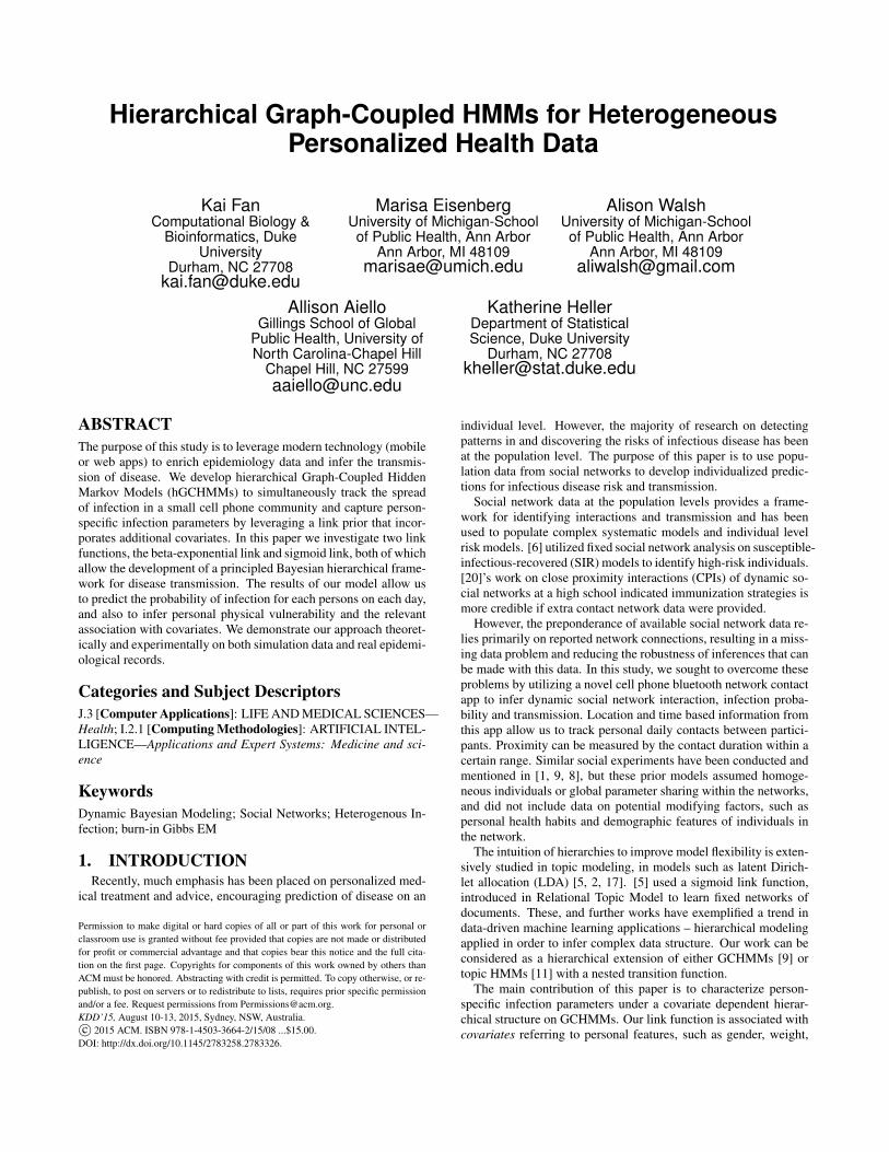
Figure 1: Illustration of GCHMMs including 3 people. 1 and 3have social contact between t− 1 and t. The infection states of1 and 3 at t are then both influenced by each others’ infectionstates at time t− 1.

hygiene habits, and diet habits, with the hypothesis that better per-sonal hygiene, diet, and lower weight, should be result in lowersusceptibility to influenza. However, it is difficult to choose an ap-propriate link function or distribution to obtain a conjugate priorfor inference. Our proposed link function can be easily generalizedto Dirichlet-exponential or softmax link. Inspired by [7], a burn-in Gibbs sampling Expectation Maximization (bGEM) algorithmis developed for parameter estimation in hGCHMMs, and addi-tional infection network inference simultaneously. Specifically, afaster version of our EM algorithm when binary latent variablesare appropriate is primarily used for our experimental tests, whichsignificantly accelerates the computational speed without a signif-icant impact on accuracy. In the case of unavailable covariates,our model is easily reduced to a no-link version by simply infer-ring each infection parameter from a common prior, the same as instandard GCHMMs.

The rest of the paper is organized as follows. In Sec. 2, we de-scribe the basic idea of GCHMMs and our proposed hGCHMMs,explicitly discussing the two different link schemes. In Sec. 3, weshow how to modify the EM algorithm for a burn-in Gibbs sam-pling version. In Sec. 4, we report empirical results by imple-menting our algorithm and applying it to synthetic and real-worlddatasets. Conclusions and future research directions are discussedin Sec. 5.

2. GENERATIVE MODELINGWe first briefly introduce the standard graph-coupled hidden Markov

model (GCHMM) (evolving from coupled hidden Markov model[3]), a dynamic model for analyzing the discrete-time series databy leveraging the interactions of a non-fixed social network (seeFigure 1 for an example, where filled in nodes are observed).

2.1 Graph-Coupled Hidden Markov ModelsLet Gt = (N,Et) be a network structure at time t, where each

agent or participant is represented by a node n ∈ N in graph Gt,

Notationsn ∈ [N ] index for participantst ∈ [T ] index for timestamps ∈ [S] index for symptoms of observationzn covariates indicating personal featuresGt−1 dynamic social networks between t− 1 and tγ(γn) recovery probability if infectious at previous timestampα(αn) probability being infected from some one outside networksβ(βn) probability being infected from some one inside networksξ infection probability of initial hidden state xn,1

xn,t ∈ X = {0, 1} latent variable indicates whether infectionyn,t ∈ Y = {0, 1}S reported symptoms during each time interval

θxn,t,s emission probability of symptom s onset given xn,t

and Et is a set of undirected edges in Gt, where (ni, nj) ∈ Et iftwo participants ni and nj have a valid contact between time t andt+ 1. The generative model of GCHMMs is then defined in a fullybayesian way (Notations in above Table).

ξ ∼ Beta(aξ, bξ) α ∼ Beta(aα, bα)

β ∼ Beta(aβ , bβ) γ ∼ Beta(aγ , bγ)

θ0,s ∼ Beta(a0, b0) θ1,s ∼ Beta(a1, b1)

xn,0 ∼ Bernoulli(ξ)

xn,t ∼ Bernoulli(φn,xn′ :(n,n′)∈Gt(α, β, γ)

)yn,t,s ∼ Bernoulli(θxn,t,s)

(1)

where the transition probability φn,xn′ :(n,n′)∈Gt(α, β, γ) is a func-tion of the infection parameters and the dynamic graph structure.Figure 1 also indicates that the transition of the hidden state is notonly dependent on the previous state of its own HMM but also influ-enced by states from other HMMs that have edges connected to it.One undirected edge inGt indicates a valid contact in time interval[t, t + 1], thus leading to a directed edge in GCHMMs. Recallingthe definition in terms of γ, α, β, we have the transition probabilityas follows:

φn,xn′ :(n,n′)∈Gt(γ, α, β) =γ xn,t = 1, xn,t+1 = 0;

1− γ xn,t = 1, xn,t+1 = 1;1− (1− α)(1− β)Cn,t xn,t = 0, xn,t+1 = 1;

(1− α)(1− β)Cn,t xn,t = 0, xn,t+1 = 0.

(2)

where Cn,t =∑n′:(n′,n)∈Et I{xn′,t=1} is the count of possible

infectious sources for node n in Gt, and I{} is the indicator func-tion. This Bayesian formulation of the GCHMMs can be applied tofit homogenous susceptible-infectious-susceptible (SIS) epidemicdynamics. Next we will generalize this basic model for other re-lated purposes by leveraging hierarchical structure and the relevantcovariates.

2.2 Extending GCHMMs to HierarchiesIt is assumed that personal health features (covariates) are present,

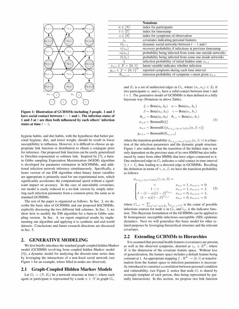
as well as the observed symptoms, denoted as zn ∈ RK , whereK is the dimension of the covariate feature space. Without lossof generalization, the feature space includes a default feature beingconstant at 1. An appropriate mapping f : RK → [0, 1] or transfor-mation from the feature space to infection parameters is necessar-ily introduced to construct a correlation between personal conditionand vulnerability, (see Figure 2, notice that node Gt is shared byrectangle template of each person, thus being represented by par-tially intersection). In this section, we propose two link function

θX

h

xn,t−1 xn,t xn,t+1

yn,t−1 yn,t yn,t+1

γn, αn, βn zn

η

Gt−1 Gt

N

Figure 2: Template Representation of hGCHMM: The graphi-cal model renders a clear structure visualization on the depen-dence between all variables and parameters.

constructions. A natural way to go is to extend the beta prior of thestandard GCHMM to a beta-exponential link.

Beta-exponential link

η·,· ∼ N(µ,Σ)

γn ∼ Beta(exp(z>n ηr,1), exp(z>n ηr,2))

αn ∼ Beta(exp(z>n ηa,1), exp(z>n ηa,2))

βn ∼ Beta(exp(z>n ηb,1), exp(z>n ηb,2))

where η·,· is distributed as multivariate Gaussian playing the role ofthe regression coefficients, since the expectation 1

1+ez>n (η·,1−η·,2)

can be considered as an approximation for logistic regression withcoefficients −(η·,1 − η·,2). This link also enables the exponentialterm exp(z>n η·,·) to take the place of the hyper-parameter of betaprior. The usual count update to the hyper-parameter will implicitlyupdate η via our EM algorithm.

Once γ, α, β are allowed to be indexed by n, the arguments inEquation (2) need index modification, but the other terms remainthe same. We put an individual level distribution on transition butnot on emission because it makes more sense that everyone hasthe same probability of physical behavior given an infection state.Patients should have corresponding symptoms, such as cough orthroat pain, or the flu cannot be discovered or diagnosed. The ad-vantage of this setting is that it allows for the Gibbs sampling ofinfection parameters in a way that still holds from previous models,except for η, so that the original Gibbs sampling scheme to updatethe beta distribution by event counts is the same in the later E-step.Another advantage is, when X is generalized to categorical vari-ables, a similar construction also works. Furthermore, rather thando approximate logistic regression, we next propose a real logisticregression link.

Sigmoid link

η· ∼ N(µ,Σ)

γn = σ(z>n ηr), αn = σ(z>n ηa), βn = σ(z>n ηb)

where σ(x) = 11+e−x is the sigmoid function.

In the generative process of infection parameters, less ηs arepresent, thus leading to a simpler model. Instead of sampling, theequations for γ, α, β will actually make these parameters vanishin the model. In other words, φn,xn′ :(n,n′)∈Gt(γn, αn, βn) is re-placed by φn,xn′ :(n,n′)∈Gt(zn, η·, σ(·)). From an implementationperspective, the EM derivation will be easier, and the experimental

results imply its outperformance of competing methods. Addition-ally, this link function inspires another two-step model: first, theinfection parameters in Equation (1) are enforced to be individuallyindexed by n, and the inference process is run in a similar Gibbssampling scheme [9]; second, a standard logistic regression is fitbetween the learned individual parameters and covariates Z.

Remark (1) The beta-exponential generative model is not welldefined for one time step data simulation, because we need a uniquesample from this generative model, which actually uses a set offixed parameters (αfn, β

fn, γ

fn)Nn=1 to sample X and Y . Take γn

for example, E(γn) 6= γfn , since γfn is one realization of the gen-erative model. What our algorithm aims to learn is a generativedistribution Beta(ez

>n ηr,1 , ez

>n ηr,2), with expectation equal to γfn ,

not E(γn). (2) Therefore, our simulation dataset is always gen-erated from the sigmoid link model. However, it is reasonable touse the beta-exponential link model for inference to eliminate theinconsistency. It has been mentioned previously the expectation ofbeta-exponential is virtually an approximation logistic regression.An EM like algorithm can perform a good point estimation for thisexpectation, which in turn would be an estimator of the sigmoidlink. (3) Another way to make the beta-exponential generative andthe inference process work is to sample αn, βn, γn both individu-ally and dynamically, i.e. γn,t, αn,t, βn,t. A number of realizationsare sufficient to learn the true generative distribution, though thenew inference algorithm will necessarily become more difficult.

Another interpretation of βn In above two extensions, it is im-plicitly assumed that βn means the individual infection probabilityfrom another person within the network, is as given in Equation(3). From the biological side, the contagiousness of the infectedperson varies, meaning that βn can be interpreted as the probabil-ity of spreading illness to any other person in the social network.This interpretation results in a slightly complicated mathematicalcalculation (details in EM algorithm section), since both the totalcount of infectious contacts and specific diffusion sources are re-quired for Equation (4).

P (xn,t+1 = 1|xn,t = 0) = 1− (1− αn)(1− βn)Cn,t (3)

P (xn,t+1 = 1|xn,t = 0) = 1− (1− αn)∏

n′∈Sn,t

(1− βn′) (4)

where the nodes set of infection contacts is defined as Sn,t ={n′ ∈ [N ] : (n, n′) ∈ Et, xn′,t = 1}.

3. INFERENCE

3.1 Approximate Conjugate for Beta-exponentiallink

The inference process is designed to invert the generative modeland to discover the η and X that best explain G and Y . In our hi-erarchical extension, however, a fully conjugate prior is not presentand it has been mentioned that knowing what the right prior is canbe difficult. Thus an approximate conjugate is developed by in-troducing the auxiliary variable Rn,t, representing the non-specificinfection source (inside or outside networks). The idea is to decom-pose infection probability 1− (1−αn)(1−βn)Cn,t into the sum-mation of three terms, αn(1−βn)Cn,t , (1−αn)(1−(1−βn)Cn,t)and αn(1−(1−βn)Cn,t), indicating infection from outside, insideand both respectively. Rn,t follows categorical distribution:

P (Rn,t) =

αn(1−βn)Cn,t

1−(1−αn)(1−βn)Cn,t, if Rn,t = 1

(1−αn)(1−(1−βn)Cn,t )1−(1−αn)(1−βn)Cn,t

, if Rn,t = 2

α(1−(1−βn)Cn,t )1−(1−αn)(1−βn)Cn,t

, if Rn,t = 3

(5)

The exact distribution of Rn,t is still difficult to use. Thus bytaylor expansion we have P (Rn,t = 2)P (xn,t+1 = 1|xn,t =0) ≈ Cn,t(1 − αn)βn and P (Rn,t = 3)P (xn,t+1 = 1|xn,t =0) ≈ Cn,tαnβn. The two approximations attain the fact that lo-cal full conditionals can be analytically obtained by discarding ηtemporarily. In practice the term involving P (Rn,t = 3) can beapproximated as 0 for Gibbs sampling. Because of the biologicalapplication, αn and βn are both the positive real value close to 0,resulting in their product being quite small. Even if this probabilityis taken into consideration in the Gibbs sampling, there is a verysmall chance that Rn,t = 3. This approximation allows the poste-rior distribution of αn, βn to be much easier to compute given thecurrent value of η. Concretely, we have the following posteriors,which will benefit the EM algorithm described later:

αn ∼ Beta(ez>n ηa,1 + Cn,Rn=1,3, e

z>n ηa,2 + Cn,Rn=2 + Cn,0→0

)βn ∼ Beta

(ez>n ηb,1 + Cn,Rn=2,3, e

z>n ηb,2 + Cn,R 6=2,3

)γn ∼ Beta(ez

>n ηr,1 + Cn,1→0, e

z>n ηr,2 + Cn,1→1)

where the count notations are defined as follows.

Cn,i→j =∑t I{xn,t=i,xn,t+1=j}, i, j ∈ {0, 1}

Cn,Rn=1,3 =∑t I{Rn,t=1,3} ≈ Cn,Rn=1 =

∑t I{Rn,t=1}

Cn,Rn=2,3 =∑t I{Rn,t=2,3} ≈ Cn,Rn=2 =

∑t I{Rn,t=2}

Cn,R 6=2,3 =∑t Cn,t

[I{Rn,t=1} + I{xn,t=0,xn,t+1=0}

]Note that auxiliary variable R did not appear in the posterior of

γn, which is exactly computed due to conjugacy. Utilizing theseapproximate posteriors, the complete likelihood P (X,R, η|Z) isobtained by integrating out the infection parameters.∫

P (R|X,α, β)P (X|γ, α, β)P (γ, α, β|η, Z)P (η)dγdαdβ

=P (η)∏n

(B(ez

>n ηr,1 + Cn,1→0, e

z>n ηr,2 + Cn,1→1)

B(ez>n ηr,1 , ez

>n ηr,2)

· B(ez>n ηa,1 + Cn,Rn=1,3, e

z>n ηa,2 + Cn,Rn=2 + Cn,0→0)

B(ez>n ηa,1 , ez

>n ηa,2)

· B(ez>n ηb,1 + Cn,Rn=2,3, e

Z>n ηb,2 + Cn,R 6=2,3)

B(ez>n ηb,1 , ez

>n ηb,2)

)(6)

where B(·) is beta function, and P (η) is a multinomial Gaussiandistribution. The integral result enables the analytical computationof the gradient ∇η and Hessian ∂2 of the log-likelihood, then con-tributing to Newton’s method.

3.2 Gibbs Sampling for Conjugate PartSampling Infection States Given all αn, βn, γn, the generative

model implies a conjugate prior for xn,t. The unnormalized poste-rior probability of xn,t = i can be represented as pin,t, i = 0, 1.

p0n,t ∝∏s

θI(yn,t,s=1)

0,s (1− θ0,s)I(yn,t,s=0) × γI(xn,t−1=1)

n (7)

·(

1− (1− αn)(1− βn)Cn,t)I(xn,t+1=1)

· (1− αn)I{xn,t−1=0,xn,t+1=0}

(1− βn)Cn,t−1I(xn,t−1=0)+Cn,tI(xn,t+1=0)

p1n,t ∝∏s

θI(yn,t,s=1)

1,s (1− θ1,s)I(yn,t,s=0) (8)

γI(xn,t+1=0)

n · (1− γn)I{xn,t−1=1,xn,t+1=1}

·(

1− (1− αn)(1− βn)Cn,t−1

)I(xn,t−1=0)

where the normalized posterior of p(xn,t = 1) isp1n,t

p0n,t+p1n,1

. There

needs to be some caution of the boundary condition since xn,1and xn,T do not have this form. xn,1 is generated by xn,1 ∼Bernoulli(ξ), where ξ ∼ Beta(aξ, bξ). The full conditional de-pends on the initial event occurrence rate ξ, further requiring somemild modification. The full conditional of ξ can be computed.

ξ|X ∼ Beta

(aξ +

∑n

I(xn,1=1), bξ +N −∑n

I(xn,1=1)

)For state xn,T , the posterior is easily computed since terms associ-ated with t+ 1 cancel out immediately.

Sampling Missing Observation For real world data, a missingvalue problem commonly arises because of underreporting in datacollection. Bayesian schemes can successfully fill in missing val-ues by drawing yn,t,s according to the distribution Bernoulli(θxn,t,s),if they are NA. Sampling yn,t,i, the posterior of θi,s, (i = 0, 1) isfrom a beta distribution.

θi,s|X,Y ∼ Beta

(ai +

∑n,t

I{yn,t,s=1,xn,t=i}, bi +∑n,t

I{yn,t,s=0,xn,t=i}

)

3.3 Burn-in Gibbs EM AlgorithmAs far as we know, previous works on CHMMs or GCHMMs

have not included the sampling scheme for global parameters η.One possible solution is the Metropolis Hastings (MH) algorithmdue to the approximate likelihood in Equation (6); however, thetransition kernel is difficult to choose for MH, and running largenumbers of iterations is usually required to achieve good mixing.

In this section, we propose a fast algorithm based on expectation-maximization. Expected sufficient statistics are computationallyintractable since there is no closed form in our case. StochasticApproximation (SA) EM [7] is an alternative introduced to sim-ulate the expectation, and able to obtain convergence to a localminimum with a theoretical guarantee under mild conditions. Thebasic idea of this computation is using a Monte Carlo sampling ap-proximation; however, we replace this step with Gibbs sampling byutilizing the approximate conjugacy property.

E-step: Sampling {X(j)}Jj=1 and {R(j)}Jj=1 follows

αn, βn, γn|Z, η(k−1) (9)X|αn, βn, γn, YR|X,αn, βn, γn, G

The true expectation integration Q(k)(η) is approximately calcu-lated by a stochastic averaging in a burn-in representation Q(k)(η),taking advantage of Gibbs sampling with form (11). During eachGibbs sampling step, infection parameters are in fact always up-dated at each inner iteration, thus making the latent variables X,Rupdate based on different posterior distributions at each sampling,which disagrees with SAEM. Therefore the samples at later iter-ations are closer to the true posterior given current η(k−1). Inordinary SAEM, latent variables are sampled from a fixed poste-rior, which is the reason why burn-in modification is not necessary.From this perspective, the burn-in Gibbs sampling in E-step mayaccelerate the convergence rate in the next maximization step.

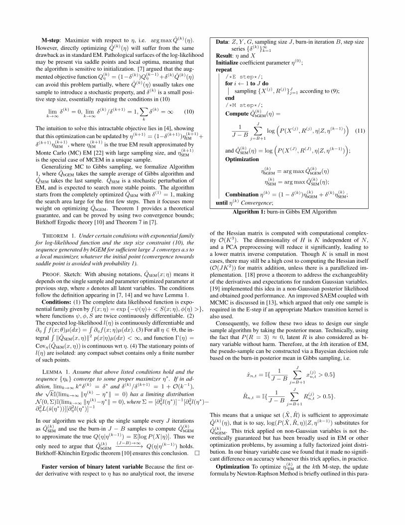
M-step: Maximize with respect to η, i.e. arg max Q(k)(η).However, directly optimizing Q(k)(η) will suffer from the samedrawback as in standard EM. Pathological surfaces of the log-likelihoodmay be present via saddle points and local optima, meaning thatthe algorithm is sensitive to initialization. [7] argued that the aug-mented objective functionQ(k)

η = (1−δ(k))Q(k−1)η +δ(k)Q(k)(η)

can avoid this problem partially, where Q(k)(η) usually takes onesample to introduce a stochastic property, and δ(k) is a small posi-tive step size, essentially requiring the conditions in (10)

limk→∞

δ(k) = 0, limk→∞

δ(k)/δ(k+1) = 1,∑k

δ(k) =∞ (10)

The intuition to solve this intractable objective lies in [4], showingthat this optimization can be updated by η(k+1) = (1−δ(k+1))η

(k+1)EM +

δ(k+1)η(k+1)SEM , where η(k+1)

EM is the true EM result approximated byMonte Carlo (MC) EM [22] with large sampling size, and η(k+1)

SEMis the special case of MCEM in a unique sample.

Generalizing MC to Gibbs sampling, we formalize Algorithm1, where QbGEM takes the sample average of Gibbs algorithm andQSEM takes the last sample. QSEM is a stochastic perturbation ofEM, and is expected to search more stable points. The algorithmstarts from the completely optimized QSEM with δ(1) = 1, makingthe search area large for the first few steps. Then it focuses moreweight on optimizing QbGEM. Theorem 1 provides a theoreticalguarantee, and can be proved by using two convergence bounds;Birkhoff Ergodic theory [10] and Theorem 7 in [7].

THEOREM 1. Under certain conditions with exponential familyfor log-likelihood function and the step size constraint (10), thesequence generated by bGEM for sufficient large J converges a.s toa local maximizer, whatever the initial point (convergence towardssaddle point is avoided with probability 1).

PROOF. Sketch: With abusing notations, QSEM(x; η) means itdepends on the single sample and parameter optimized parameter atprevious step, where s denotes all latent variables. The conditionsfollow the definition appearing in [7, 14] and we have Lemma 1.

Conditions: (1) The complete data likelihood function is expo-nential family given by f(x; η) = exp {−ψ(η)+ < S(x; η), φ(η) >},where functions ψ, φ, S are twice continuously differentiable. (2)The expected log-likelihood l(η) is continuously differentiable and∂η∫f(x; θ)µ(dx) =

∫∂ηf(x; η)µ(dx). (3) For all η ∈ Θ, the in-

tegral∫‖QSEM(x, η)‖2 p(x|η)µ(dx) < ∞, and function Γ(η) =

Covη(QSEM(x, η)) is continuous wrt η. (4) The stationary points ofl(η) are isolated: any compact subset contains only a finite numberof such points.

LEMMA 1. Assume that above listed conditions hold and thesequence {ηk} converge to some proper maximizer η∗. If in ad-dition, limk→∞ k

aδ(k) = δ∗ and δ(k)/δ(k+1) = 1 + O(k−1),the√kI(limk→∞ ‖η(k) − η∗‖ = 0) has a limiting distribution

N (0,Σ)I(limk→∞ ‖η(k)−η∗‖ = 0), where Σ = [∂2ηl(η

∗)]−1[∂2ηl(η

∗)−∂2ηL(s(η∗))][∂2

ηl(η∗)]−1

In our algorithm we pick up the single sample every J iterationsas Q(k)

SEM and use the burn-in J − B samples to compute Q(k)bGEM

to approximate the true Q(η|η(k−1)) = E[logP (X|η)]. Thus we

only need to argue that Q(k)bGEM

(J−B)→∞−−−−−−−→ Q(η|η(k−1)) holds.Birkhoff-Khinchin Ergodic theorem [10] ensures this conclusion.

Faster version of binary latent variable Because the first or-der derivative with respect to η has no analytical root, the inverse

Data: Z, Y , G, sampling size J , burn-in iteration B, step sizeseries {δ(k)}∞k=1

Result: η and XInitialize coefficient parameter η(0);repeat

/*E step*/;for i← 1 to J do

sampling {X(j), R(j)}Jj=1 according to (9);end/*M step*/;Compute Q(k)

bGEM(η) =

1

J −B

J∑j=B+1

log(P (X(j), R(j), η|Z, η(k−1))

)(11)

and Q(k)SEM(η) = log

(P (X(J), R(J), η|Z, η(k−1))

);

Optimization

η(k)bGEM = arg max Q

(k)bGEM(η)

η(k)SEM = arg max Q

(k)SEM(η);

Combination η(k) = (1− δ(k))η(k)bGEM + δ(k)η(k)SEM;

until η(k) Convergence;Algorithm 1: burn-in Gibbs EM Algorithm

of the Hessian matrix is computed with computational complex-ity O(K3). The dimensionality of H is K independent of N ,and a PCA preprocessing will reduce it significantly, leading toa lower matrix inverse computation. Though K is small in mostcases, there may still be a high cost to computing the Hessian itself(O(JK2)) for matrix addition, unless there is a parallelized im-plementation. [18] prove a theorem to address the exchangeablityof the derivatives and expectations for random Gaussian variables.[19] implemented this idea in a non-Gaussian posterior likelihoodand obtained good performance. An improved SAEM coupled withMCMC is discussed in [13], which argued that only one sample isrequired in the E-step if an appropriate Markov transition kernel isalso used.

Consequently, we follow these two ideas to design our singlesample algorithm by taking the posterior mean. Technically, usingthe fact that P (R = 3) ≈ 0, latent R is also considered as bi-nary variable without harm. Therefore, at the kth iteration of EM,the pseudo-sample can be constructed via a Bayesian decision rulebased on the burn-in posterior mean in Gibbs sampling, i.e.

xn,t = I{ 1

J −B

J∑j=B+1

x(j)n,t > 0.5}

Rn,t = I{ 1

J −B

J∑j=B+1

R(j)n,t > 0.5}.

This means that a unique set (X, R) is sufficient to approximateQ(k)(η), that is to say, log(P (X, R, η)|Z, η(k−1)) substitutes forQ

(k)bGEM. This trick applied on non-Gaussian variables is not the-

oretically guaranteed but has been broadly used in EM or otheroptimization problems, by assuming a fully factorized joint distri-bution. In our binary variable case we found that it made no signifi-cant difference on accuracy whenever this trick applies, in practice.

Optimization To optimize η(k)*EM at the kth M-step, the updateformula by Newton-Raphson Method is briefly outlined in this para-

graph, excluding the analytical gradient G and Hessian H compu-tation. For efficiency, we update parameters as follows, with a fewiterations.

η(k)*EM:new = η

(k)*EM:old − δH

−1G

where *EM varies according to different estimators, bGEM or SEM.It is unnecessary for there to be complete convergence in order toguarantee Q(η(k)) > Q(η(k−1)). A similar idea with a single iter-ation is mentioned in [14]. The step size δ ensures that the Wolfeconditions [16] are satisfied. The intuition in adding in step sizehere is, compared with gradient descent, Newton’s Method tendsto make more progress in the right direction of local optima, dueto the property of affine invariance. This probably leads an updatewhere the step size is too large, so it is better for stochastic algo-rithms to enlarge the search domain at first then shrink later.

3.4 Simpler Algorithm on Sigmoid linkAs has been previously discussed, a sigmoid link function ben-

efits from model simplicity and hiding infection parameters with-out integrating them out. The likelihood P (η,X|Z) can thus beexactly computed as Equation (12). It means that, in parameterestimation, we can either apply standard SAEM by getting rid oflatent variable R immediately, or bGEM by introducing R as wellin E-step and faster version M-step by keeping X alone.

P (η)

N∏n=1

P (xn,1)×N∏n=1

T−1∏t=1

(12)

σ(z>n ηr)I{xn,t=1,xn,t+1=0}

(1− σ(z>n ηr)

)I{xn,t=1,xn,t+1=1}

·(

1− (1− σ(z>n ηa))(1− σ(z>n ηb))Cn,t

)I{xn,t=0,xn,t+1=1}

·(

(1− σ(z>n ηa))(1− σ(z>n ηb))Cn,t

)I{xn,t=0,xn,t+1=0}.

3.5 Discussion on Another InterpretationIn the second biological interpretation of βn (probability of in-

fecting others), transition function φn,xn′ :(n,n′)∈Gt will depend onthe extra parameter set {βn′ : n′ ∈ Sn,t}. Consequently, the pos-terior of each βn requires both a count number and source tracking(like the concept of a "pointer" in the C programming language).However, the likelihood of the beta-exponential model can be sim-plified to integrate out these parameters due to the auxiliary vari-able R as well, corresponding to the new categorical distributionin Equation (13), though P (R) in Equation (5) can also have thisformulation.

P (Rn,t) ≈ Cat

(αn∏n′∈Sn,t(1− βn′)

1− (1− αn)∏n′∈Sn,t(1− βn′)

,

(1− αn)βn′

1− (1− αn)∏n′∈Sn,t(1− βn′)

, . . .

)(13)

P (X,R, η|Z) = P (η)∏n

(B(ez

>n ηr,1 + Cn,1→0, e

z>n ηr,2 + Cn,1→1

B(ez>n ηr,1 , ez

>n ηr,2)

· B(ez>n ηa,1 + Cn,Rn=0, e

z>n ηa,2 + Cn,Rn 6=0 + Cn,0→0

B(ez>n ηa,1 , ez

>n ηa,2)

· B(ez>n ηb,1 + Cn,R=n, e

z>n ηb,2 + Cn,R 6=n

B(ez>n ηb,1 , ez

>n ηb,2)

)(14)

Rn,t takes the value {0, 1, ..., Cn,t}, where 0 means there is an out-side network source and other integers mean specific infection in-

network sources. The categorical distribution makes the beta priorfor the infection parameters conjugate in the posterior. However,the integral for the likelihood is actually difficult and needs somealgebraic tricks, especially for βn because of the source tracking.We show the result of the beta-exponential model in 14, while thesigmoid model is straightforward and obtained without too manytricks. The new count notations are listed below.

Cn,Rn=0 =∑t I{Rn,t=0}

Cn,Rn 6=0 =∑t

∑n′∈Sn,t I{Rn,t=n′}

Cn,R=n =∑n′,t:n∈Sn′,t

I{Rn′,t=n}Cn,R 6=n =

∑n′,t:n∈Sn′,t

[I{Rn′,t=0} + I{xn′,t=0,xn′,t+1=0}]

4. EXPERIMENTAL RESULTSIn this section we illustrate, on simulated data, the performance

of our approach, hGCHMMs and the burn-in Gibbs EM algorithmon three datasets for the purposes of predicting the hidden infec-tious state X , filling in missing data – observation Y , and infer-ring an individual’s physical condition based on parameter estima-tion. Further application on the public real world Social EvolutionDataset [15] and our mobile apps survey dataset are also shown.

4.1 Semi-Simulation Dataset

4.1.1 Data GenerationDiffering from completely simulated data or a totally artificial

setting, we employed a generative model to synthesize X ,Y basedon the real dynamic social network Gt and covariates Z from thereal Social Evolution dataset. The predefined X then plays the roleof ground truth, making evaluation for all above points possible.

Real Part Public MIT Social Evolution dataset contains the dy-namic networks G including 84 participants over 107 days, Gt in-dexes 1 to 107, and covariates zn exist for each participant, includ-ing 9 features, weight, height, salads per week, veggies fruits perday, healthy diet level, aerobics per week, sports per week, smok-ing indicator, and default feature 1. The quantity per week is fre-quency. Weight and height are taken as real values. Healthy dietincludes 6 levels ranging from very unhealthy to very healthy basedon self evaluation. Smoking indicator is literally a binary variable.Real symptoms Y are temporarily discarded since the true infectionstates X are unavailable for this dataset.

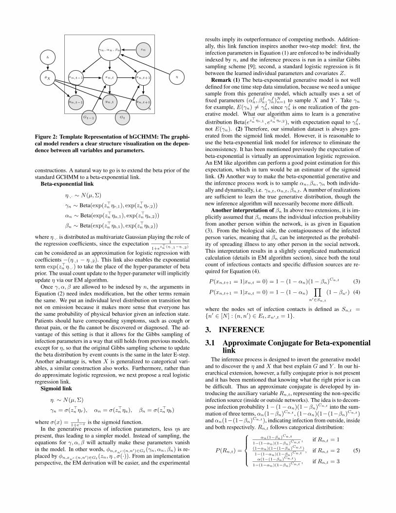
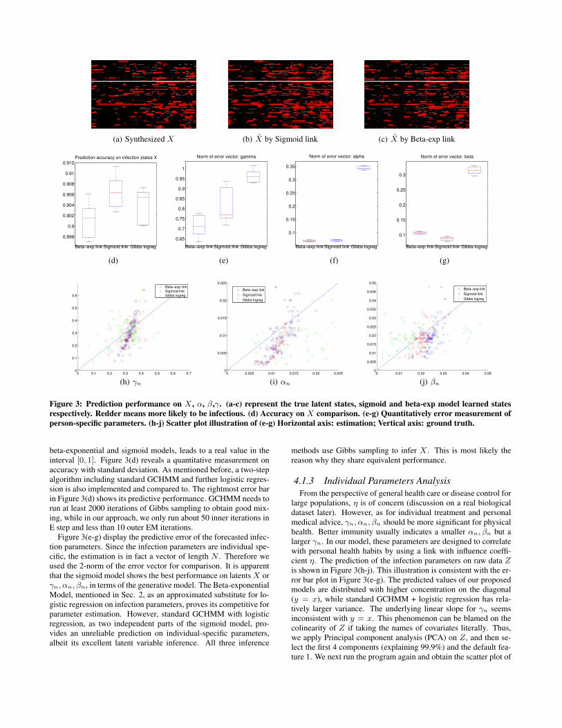
Synthesized Part X and Y are then generated based on a Sig-moid link generative model. It is noticed that hyperparamter ηneeds to be predefined, which means synthesized infection param-eters γn, αn, βn are known because of the sigmoid function. Onlysynthesized data Y with 6 symptoms is given to learning model, butthe evaluation is done on other variables. The proportion of miss-ing values in Y is set to 0.5, i.e, the observations yn,t,s are NA withprobability 0.5. Our generated X (an 84 × 108 matrix, includinginitial states) is shown in Figure 3(a). Each row vector represents aperson’s infection states during the entire observation period.

4.1.2 Model EvaluationWe ran the algorithm 10 times. The prediction performance on

latent variable X is the byproduct of the E-step, and when xn,t islarger than the threshold 0.5 the person is diagnosed as being in-fected. Since X is completely unknown to the algorithm, held-outtest data prediction is unnecessary but allX is used to evaluate pre-diction accuracy. Figure 3(a-c) shows the difference between thetruth and the inferred results from each of the two linked models.The posterior mean from Gibbs sampling for prediction, in both

(a) Synthesized X (b) X by Sigmoid link (c) X by Beta-exp link

0.898

0.9

0.902

0.904

0.906

0.908

0.91

0.912

Beta−exp link Sigmoid link Gibbs logreg

Prediction accuracy on infection states X

(d)

0.65

0.7

0.75

0.8

0.85

0.9

0.95

1

Beta−exp link Sigmoid link Gibbs logreg

Norm of error vector: gamma

(e)

0.1

0.15

0.2

0.25

0.3

0.35

Beta−exp link Sigmoid link Gibbs logreg

Norm of error vector: alpha

(f)

0.1

0.15

0.2

0.25

0.3

Beta−exp link Sigmoid link Gibbs logreg

Norm of error vector: beta

(g)

0 0.1 0.2 0.3 0.4 0.5 0.6 0.70

0.1

0.2

0.3

0.4

0.5

0.6

Beta−exp link

Sigmoid link

Gibbs logreg

(h) γn0 0.005 0.01 0.015 0.02 0.025

0

0.005

0.01

0.015

0.02

0.025

Beta−exp link

Sigmoid link

Gibbs logreg

(i) αn0 0.01 0.02 0.03 0.04 0.05

0

0.005

0.01

0.015

0.02

0.025

0.03

0.035

0.04

0.045

0.05

Beta−exp link

Sigmoid link

Gibbs logreg

(j) βn

Figure 3: Prediction performance on X , α, β,γ. (a-c) represent the true latent states, sigmoid and beta-exp model learned statesrespectively. Redder means more likely to be infectious. (d) Accuracy on X comparison. (e-g) Quantitatively error measurement ofperson-specific parameters. (h-j) Scatter plot illustration of (e-g) Horizontal axis: estimation; Vertical axis: ground truth.

beta-exponential and sigmoid models, leads to a real value in theinterval [0, 1]. Figure 3(d) reveals a quantitative measurement onaccuracy with standard deviation. As mentioned before, a two-stepalgorithm including standard GCHMM and further logistic regres-sion is also implemented and compared to. The rightmost error barin Figure 3(d) shows its predictive performance. GCHMM needs torun at least 2000 iterations of Gibbs sampling to obtain good mix-ing, while in our approach, we only run about 50 inner iterations inE step and less than 10 outer EM iterations.

Figure 3(e-g) display the predictive error of the forecasted infec-tion parameters. Since the infection parameters are individual spe-cific, the estimation is in fact a vector of length N . Therefore weused the 2-norm of the error vector for comparison. It is apparentthat the sigmoid model shows the best performance on latentsX orγn, αn, βn, in terms of the generative model. The Beta-exponentialModel, mentioned in Sec. 2, as an approximated substitute for lo-gistic regression on infection parameters, proves its competitive forparameter estimation. However, standard GCHMM with logisticregression, as two independent parts of the sigmoid model, pro-vides an unreliable prediction on individual-specific parameters,albeit its excellent latent variable inference. All three inference

methods use Gibbs sampling to infer X . This is most likely thereason why they share equivalent performance.

4.1.3 Individual Parameters AnalysisFrom the perspective of general health care or disease control for

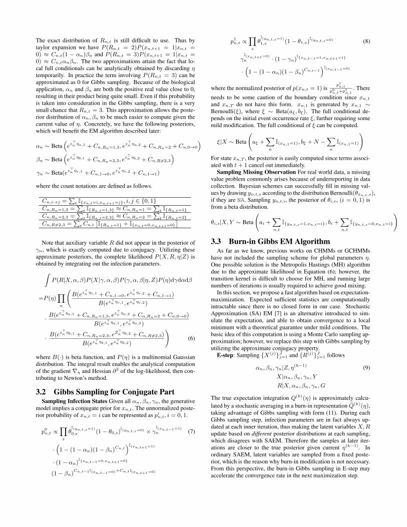
large populations, η is of concern (discussion on a real biologicaldataset later). However, as for individual treatment and personalmedical advice, γn, αn, βn should be more significant for physicalhealth. Better immunity usually indicates a smaller αn, βn but alarger γn. In our model, these parameters are designed to correlatewith personal health habits by using a link with influence coeffi-cient η. The prediction of the infection parameters on raw data Zis shown in Figure 3(h-j). This illustration is consistent with the er-ror bar plot in Figure 3(e-g). The predicted values of our proposedmodels are distributed with higher concentration on the diagonal(y = x), while standard GCHMM + logistic regression has rela-tively larger variance. The underlying linear slope for γn seemsinconsistent with y = x. This phenomenon can be blamed on thecolinearity of Z if taking the names of covariates literally. Thus,we apply Principal component analysis (PCA) on Z, and then se-lect the first 4 components (explaining 99.9%) and the default fea-ture 1. We next run the program again and obtain the scatter plot of

0 0.1 0.2 0.3 0.4 0.5 0.6 0.70

0.1

0.2

0.3

0.4

0.5

0.6

Beta−exp link

Sigmoid link

Gibbs logreg

Figure 4: Colinearity elimination on γn: PCA justification onFigure 3 (h) is to obtain the regressed slope close to 1.

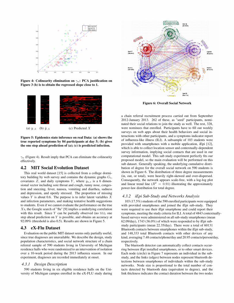
(a) y·,5 (b) y·,5 (c) Predicted X

Figure 5: Epidemics state inference on real Data: (a) shows thetrue reported symptoms by 84 participants at day 5; (b) givesthe one step ahead prediction of (a); (c) is predicted infection.

γn (Figure 4). Result imply that PCA can eliminate the colinearityeffectively.

4.2 MIT Social Evolution DatasetThis real world dataset [15] is collected from a college dormi-

tory building by web survey and contains the dynamic graphs Gt,covariates Z, and daily symptoms Y , where yn,t is a 6 dimen-sional vector including sore throat and cough, runny nose, conges-tion and sneezing, fever, nausea, vomiting and diarrhea, sadnessand depression, and openly stressed. The proportion of missingvalues Y is about 0.6. The purpose is to infer latent variables Xand infection parameters, and making tentative health suggestionsto students. Even if we cannot evaluate the performance on the trueXs, the Google search of "flu" [9] implies a underlying correlationwith this result. Since Y can be partially observed (no NA), onestep ahead prediction on Y is possible, and obtains an accuracy at92.09% (threshold is also 0.5). Results are shown in Figure 5.

4.3 eX-Flu DatasetEvaluation on the public MIT dataset seems only partially useful,

since true diagnoses are unavailable. We describe the design, studypopulation characteristics, and social network structure of a chainreferral sample of 590 students living in University of Michiganresidence halls who were randomized to an intervention of isolationover a 10-week period during the 2013 influenza season. In ourexperiment, diagnoses are recorded immediately at onset.

4.3.1 Design Description590 students living in six eligible residence halls on the Uni-

versity of Michigan campus enrolled in the eX-FLU study during

Figure 6: Overall Social Network

a chain referral recruitment process carried out from September2012-January 2013. 262 of these, as "seed" participants, nomi-nated their social relations to join the study as well. The rest, 328,were nominees that enrolled. Participants have to fill out weeklysurveys on web apps about their health behaviors and social in-teractions with other participants, and a symptoms indicator reportof influenza-like illness (ILI). A subsample of 103 students wereprovided with smartphones with a mobile application, iEpi [12],which is able to collect location sensor and contextually-dependentsurvey information, implying social contacts that are used in ourcomputational model. This sub study experiment perfectly fits ourproposed model, so the main evaluation will be performed on thissub dataset. Generally speaking, the underlying cumulative distri-bution of degree for the overall social network on 590 students isshown in Figure 6. The distribution of three degree measurements(in, out, or total), were heavily right-skewed and over-dispersed.Consequently, the network appears scale-free, with a log-log plotand linear trend line (R2 = 0.91) illustrating the approximatelypower-law distribution for total degree.

4.3.2 iEpi Sub-Study and Networks Analysis103 (17.5%) students of the 590 enrolled participants were equipped

with provided smartphones and joined the iEpi sub-study. Theywere required to use their iEpi smartphone and could report theirsymptoms, meeting the study criteria for ILI. A total of 4843 contextually-based surveys were administered on all sub-study smartphones (mean62.09/day), 1743 (36.0%) of which were responded to by iEpi sub-study participants (mean 22.35/day). There were a total of 60131Bluetooth contacts between smartphones within the iEpi sub-study,and 148,333 total Bluetooth contacts with other devices of anykind, averaging 7.48 contacts/phone/day and 20.95 contacts/person/day,respectively.

The bluetooth detector can automatically collect contacts occur-ring between iEpi installed smartphones, or to other smart devices.Each node (circle) in Figure 7 represents an individual in the sub-study, and the links (edges) between nodes represent bluetooth de-tections between smartphones of individuals within the sub-studynetworks. Node size is proportional to the total number of con-tacts detected by bluetooth data (equivalent to degree), and thelink thickness indicates the contact duration between the two nodes

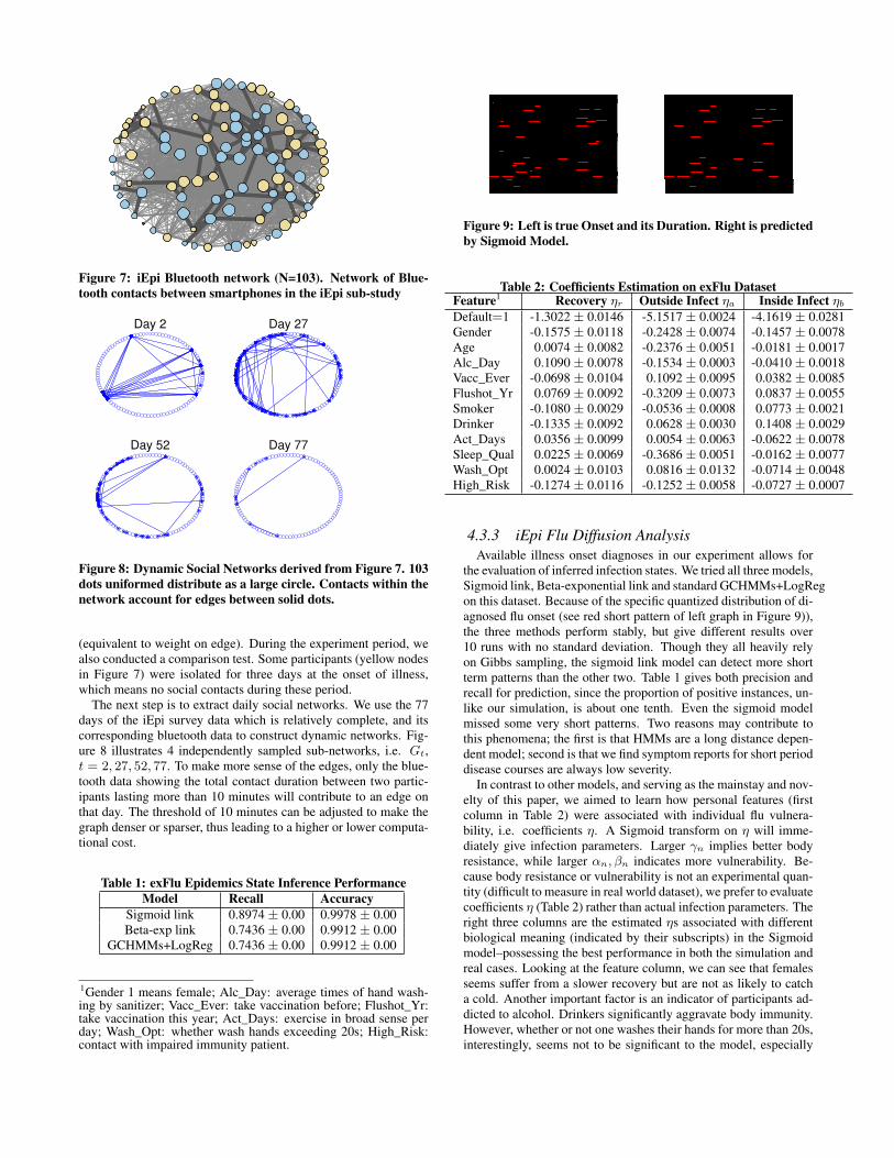
Figure 7: iEpi Bluetooth network (N=103). Network of Blue-tooth contacts between smartphones in the iEpi sub-study

Day 2 Day 27

Day 52 Day 77

Figure 8: Dynamic Social Networks derived from Figure 7. 103dots uniformed distribute as a large circle. Contacts within thenetwork account for edges between solid dots.

(equivalent to weight on edge). During the experiment period, wealso conducted a comparison test. Some participants (yellow nodesin Figure 7) were isolated for three days at the onset of illness,which means no social contacts during these period.

The next step is to extract daily social networks. We use the 77days of the iEpi survey data which is relatively complete, and itscorresponding bluetooth data to construct dynamic networks. Fig-ure 8 illustrates 4 independently sampled sub-networks, i.e. Gt,t = 2, 27, 52, 77. To make more sense of the edges, only the blue-tooth data showing the total contact duration between two partic-ipants lasting more than 10 minutes will contribute to an edge onthat day. The threshold of 10 minutes can be adjusted to make thegraph denser or sparser, thus leading to a higher or lower computa-tional cost.

Table 1: exFlu Epidemics State Inference PerformanceModel Recall Accuracy

Sigmoid link 0.8974 ± 0.00 0.9978 ± 0.00Beta-exp link 0.7436 ± 0.00 0.9912 ± 0.00

GCHMMs+LogReg 0.7436 ± 0.00 0.9912 ± 0.00

1Gender 1 means female; Alc_Day: average times of hand wash-ing by sanitizer; Vacc_Ever: take vaccination before; Flushot_Yr:take vaccination this year; Act_Days: exercise in broad sense perday; Wash_Opt: whether wash hands exceeding 20s; High_Risk:contact with impaired immunity patient.

Figure 9: Left is true Onset and its Duration. Right is predictedby Sigmoid Model.

Table 2: Coefficients Estimation on exFlu DatasetFeature1 Recovery ηr Outside Infect ηa Inside Infect ηbDefault=1 -1.3022 ± 0.0146 -5.1517 ± 0.0024 -4.1619 ± 0.0281Gender -0.1575 ± 0.0118 -0.2428 ± 0.0074 -0.1457 ± 0.0078Age 0.0074 ± 0.0082 -0.2376 ± 0.0051 -0.0181 ± 0.0017Alc_Day 0.1090 ± 0.0078 -0.1534 ± 0.0003 -0.0410 ± 0.0018Vacc_Ever -0.0698 ± 0.0104 0.1092 ± 0.0095 0.0382 ± 0.0085Flushot_Yr 0.0769 ± 0.0092 -0.3209 ± 0.0073 0.0837 ± 0.0055Smoker -0.1080 ± 0.0029 -0.0536 ± 0.0008 0.0773 ± 0.0021Drinker -0.1335 ± 0.0092 0.0628 ± 0.0030 0.1408 ± 0.0029Act_Days 0.0356 ± 0.0099 0.0054 ± 0.0063 -0.0622 ± 0.0078Sleep_Qual 0.0225 ± 0.0069 -0.3686 ± 0.0051 -0.0162 ± 0.0077Wash_Opt 0.0024 ± 0.0103 0.0816 ± 0.0132 -0.0714 ± 0.0048High_Risk -0.1274 ± 0.0116 -0.1252 ± 0.0058 -0.0727 ± 0.0007

4.3.3 iEpi Flu Diffusion AnalysisAvailable illness onset diagnoses in our experiment allows for

the evaluation of inferred infection states. We tried all three models,Sigmoid link, Beta-exponential link and standard GCHMMs+LogRegon this dataset. Because of the specific quantized distribution of di-agnosed flu onset (see red short pattern of left graph in Figure 9)),the three methods perform stably, but give different results over10 runs with no standard deviation. Though they all heavily relyon Gibbs sampling, the sigmoid link model can detect more shortterm patterns than the other two. Table 1 gives both precision andrecall for prediction, since the proportion of positive instances, un-like our simulation, is about one tenth. Even the sigmoid modelmissed some very short patterns. Two reasons may contribute tothis phenomena; the first is that HMMs are a long distance depen-dent model; second is that we find symptom reports for short perioddisease courses are always low severity.

In contrast to other models, and serving as the mainstay and nov-elty of this paper, we aimed to learn how personal features (firstcolumn in Table 2) were associated with individual flu vulnera-bility, i.e. coefficients η. A Sigmoid transform on η will imme-diately give infection parameters. Larger γn implies better bodyresistance, while larger αn, βn indicates more vulnerability. Be-cause body resistance or vulnerability is not an experimental quan-tity (difficult to measure in real world dataset), we prefer to evaluatecoefficients η (Table 2) rather than actual infection parameters. Theright three columns are the estimated ηs associated with differentbiological meaning (indicated by their subscripts) in the Sigmoidmodel–possessing the best performance in both the simulation andreal cases. Looking at the feature column, we can see that femalesseems suffer from a slower recovery but are not as likely to catcha cold. Another important factor is an indicator of participants ad-dicted to alcohol. Drinkers significantly aggravate body immunity.However, whether or not one washes their hands for more than 20s,interestingly, seems not to be significant to the model, especially

to the recovery rate. This may blamed on an overly long washingduration–20s in the experimental design. Overall, the sign consis-tency with respect to η makes sense, with the exception of a fewcounter intuitive relationships. For the sigmoid function, positivecoefficients will enlarge infection parameters, and vice versa.

5. CONCLUSIONS AND FUTURE WORKSWe propose hierarchical GCHMMs to simultaneously predict in-

dividual infection and physical constitution by observing how fluspreads within dynamic social networks. The heterogeneous modelis validated on semi-synthetic data and epidemiological trackingdata in college dormitories, and outperforms existing GCHMMs(plus logistic regression). On semi-simulation data, we evaluate ourmodel on a number of metrics, including on the ability to correctlyinfer parameters. On the MIT social evolution data, we mainlyfocus on one step ahead prediction of the observed states (or symp-toms). In our eX-Flu study, we successfully discovered the under-lying social network pattern and personal feature relationships withrespect to influenza vulnerability.

The variant of the EM algorithm we developed for inferenceproved to work well both from a theoretical view and in experimen-tal results. Future research might explore belief propagation andvariational inference methods for parameter estimation. Anotherpossible area of future research would be to implement Remark (3)or investigate infection network learning by detecting the diseasespread path (auxiliary variable R). We can further relax the het-erogeneity assumption to a cluster assumption. Inspired by HDP-HMMs [21], this tradeoff can be realized by constructing a non-parametric version GCHMMs, enforcing similar HMMs to sharethe same parameters.

6. ACKNOWLEDGMENTSWe would like to thank Dylan Knowles, under the supervision of

Dr. Nathaniel Osgood and Dr. Kevin Stanley, and the aid of otherstudents and fellows developed the iEpi application and helpedoversee the iEpi app smartphone upload, data collection proce-dures, and trouble shooting for the eXFLU study. This work wassupported by Duke NSF grant #3331830. Any opinions, findingsand conclusions or recommendations expressed in this material arethe authors’ and do not necessarily reflect those of the sponsor.

7. REFERENCES[1] R. Beckman, K. R. Bisset, J. Chen, B. Lewis, M. Marathe,

and P. Stretz. Isis: A networked-epidemiology basedpervasive web app for infectious disease pandemic planningand response. In Proceedings of the 20th ACM SIGKDDinternational conference on Knowledge discovery and datamining, pages 1847–1856. ACM, 2014.

[2] D. M. Blei, T. L. Griffiths, and M. I. Jordan. The nestedchinese restaurant process and bayesian nonparametricinference of topic hierarchies. Journal of the ACM (JACM),57(2):7, 2010.

[3] M. Brand, N. Oliver, and A. Pentland. Coupled hiddenmarkov models for complex action recognition. In ComputerVision and Pattern Recognition, 1997. Proceedings., 1997IEEE Computer Society Conference on, pages 994–999.IEEE, 1997.

[4] G. Celeux, D. Chauveau, J. Diebolt, et al. On stochasticversions of the em algorithm. 1995.

[5] J. Chang, D. M. Blei, et al. Hierarchical relational models fordocument networks. The Annals of Applied Statistics,4(1):124–150, 2010.

[6] R. M. Christley, G. Pinchbeck, R. Bowers, D. Clancy,N. French, R. Bennett, and J. Turner. Infection in socialnetworks: using network analysis to identify high-riskindividuals. American journal of epidemiology,162(10):1024–1031, 2005.

[7] B. Delyon, M. Lavielle, and E. Moulines. Convergence of astochastic approximation version of the em algorithm.Annals of Statistics, pages 94–128, 1999.

[8] W. Dong, B. Lepri, and A. S. Pentland. Modeling theco-evolution of behaviors and social relationships usingmobile phone data. In Proceedings of the 10th InternationalConference on Mobile and Ubiquitous Multimedia, pages134–143. ACM, 2011.

[9] W. Dong, A. Pentland, and K. A. Heller. Graph-coupledhmms for modeling the spread of infection. Association forUncertainty in Artificial Intelligence, 2012.

[10] R. Durrett. Probability: theory and examples. Cambridgeuniversity press, 2010.

[11] A. Gruber, Y. Weiss, and M. Rosen-Zvi. Hidden topicmarkov models. In International Conference on ArtificialIntelligence and Statistics, pages 163–170, 2007.

[12] D. L. Knowles, K. G. Stanley, and N. D. Osgood. Afield-validated architecture for the collection ofhealth-relevant behavioural data. In Healthcare Informatics(ICHI), 2014 IEEE International Conference on, pages79–88. IEEE, 2014.

[13] E. Kuhn and M. Lavielle. Coupling a stochasticapproximation version of em with an mcmc procedure.ESAIM: Probability and Statistics, 8:115–131, 2004.

[14] K. Lange. A gradient algorithm locally equivalent to the emalgorithm. Journal of the Royal Statistical Society. Series B(Methodological), pages 425–437, 1995.

[15] A. Madan, M. Cebrian, S. Moturu, K. Farrahi, andA. Pentland. Sensing the" health state" of a community.IEEE Pervasive Computing, 11(4):36–45, 2012.

[16] J. Nocedal and S. Wright. Numerical optimization, series inoperations research and financial engineering. Springer, NewYork, USA, 2006.

[17] J. Paisley, C. Wang, D. M. Blei, and M. I. Jordan. Nestedhierarchical dirichlet processes. 2012.

[18] R. Price. A useful theorem for nonlinear devices havinggaussian inputs. Information Theory, IRE Transactions on,4(2):69–72, 1958.

[19] D. J. Rezende, S. Mohamed, and D. Wierstra. Stochasticbackpropagation and approximate inference in deepgenerative models. In Proceedings of The 31st InternationalConference on Machine Learning, pages 1278–1286, 2014.

[20] M. Salathé, M. Kazandjieva, J. W. Lee, P. Levis, M. W.Feldman, and J. H. Jones. A high-resolution human contactnetwork for infectious disease transmission. Proceedings ofthe National Academy of Sciences, 107(51):22020–22025,2010.

[21] Y. W. Teh, M. I. Jordan, M. J. Beal, and D. M. Blei.Hierarchical dirichlet processes. Journal of the americanstatistical association, 101(476), 2006.

[22] G. C. Wei and M. A. Tanner. A monte carlo implementationof the em algorithm and the poor man’s data augmentationalgorithms. Journal of the American Statistical Association,85(411):699–704, 1990.