Hierarchical Bayesian Persuasion∗

Zhonghong Kuang† Jaimie W. Lien‡ Jie Zheng§

Updated July 30, 2019; First Version May 14, 2018

ABSTRACT:

We study a hierarchical Bayesian persuasion game with a sender, a receiver and several potential

intermediaries, generalizing framework of Kamenica and Gentzkow (2011, AER). The sender must

be persuasive through the hierarchy of intermediaries in order to reach the final receiver, whose

action affects all players’ payoffs. The intermediaries care not only about the true state of world and

the receiver’s action, but also about their reputations, measured by whether the receiver’s action is

consistent with their recommendation. We characterize the subgame perfect Nash equilibrium for

the optimal persuasion strategy, and show that the persuasion game has multiple equilibria but a

unique payoff outcome. Among the equilibria, two natural persuasion strategies on the hierarchy

arise: persuading the intermediary who is immediately above one’s own position, and persuading

the least persuadable individual in the hierarchy. As major extensions of the main model, we

analyze scenarios in which intermediaries have private information, the endogenous reputation

of intermediaries, and when intermediaries have an outside option. We also discuss as minor

extensions, the endogenous choice of persuasion path, parallel persuasion, and costly persuasion.

The results provide insights for settings where persuasion is prominent in a hierarchical structure,

such as corporate management, higher education admissions, job promotion, and legal proceedings.

KEYWORDS: Bayesian Persuasion, Hierarchy, Reputation, Sequential Persuasion

∗We are especially grateful to Jian Chen and Matthew Gentzkow for detailed comments which helped us to

improve the manuscript. For helpful comments and insights, we thank Masaki Aoyagi, Jimmy Chan, Bo Chen,

Zhuoqiong Chen, Fuhai Hong, Rongzhu Ke, Chiu Yu Ko, Ping Lin, Charles Noussair, Jean Tirole, Ruqu Wang, Adam

Wong, Fan Wu, Qinggong Wu, Boyu Zhang, Mu Zhang, Hangcheng Zhao, Mofei Zhao, Weijie Zhong, conference

participants at the 2018 Beijing International Workshop on Microeconomics Empirics, Experiments and Theory

(MEET 2018), 6th China Conference on Organizational Economics, 2018 Annual Conference of China Information

Economics Society, 2019 Asian Meeting of Econometric Society, 2019 China Meeting of Econometric Society and

30th Internation Conference on Game Theory, and seminar participants at Lingnan University, Tsinghua University

and Chinese University of Hong Kong. This research is funded by National Natural Science Foundation of China

(Projects No. 61661136002 and No. 71873074), Tsinghua University Initiative Scientific Research Grant (Project

No. 20151080397), Tsinghua University Tutor Research Fund, and Chinese University of Hong Kong Direct Grants.

All errors are our own.†Zhonghong Kuang: Department of Management Science and Engineering, School of Economics and Management,

Tsinghua University, Beijing, China (email: kuangzhh.15@sem.tsinghua.edu.cn).‡Jaimie W. Lien: Department of Decision Sciences and Managerial Economics, CUHK Business School, The

Chinese University of Hong Kong, Hong Kong SAR, China (email: jaimie.academic@gmail.com).§Jie Zheng (Corresponding Author): Department of Economics, School of Economics and Management, Tsinghua

University, Beijing, China, 100084 (e-mail: jie.academic@gmail.com).

1

JEL CLASSIFICATION: C72, C73, D82, D83

2

1 Introduction

An individual hoping to persuade a decision-making authority in the direction of his or her

preferred outcome often does not have direct access to that person-in-charge. An entry level worker

at a company may have a profitable idea, but he can neither implement it himself nor persuade

the CEO directly. Instead, he must persuade his manager, who if persuaded, persuades his own

manager, and so on through the corporate hierarchy until a decision-making authority is convinced.

Similar persuasion structures are commonplace whenever the incentive to persuade originates

from the bottom of a hierarchy, upward. When applying for graduate school, students must

convince their professors that they are suitable for future study, who if well-convinced, write

recommendation letters to convince admissions committees to admit the student. Similarly, job

promotion processes in academia settings often require an endorsement at the department level,

followed by the faculty or division level, and so on, before being approved at the university level.

We study the persuasion strategies and equilibrium characteristics in a hierarchical version

of Kamenica and Gentzkow’s (2011) Bayesian persuasion model. In their framework, which is

increasingly applied to a variety of settings in the literature, a sender with a strictly preferred

outcome over a receiver’s actions, commits to a conditional signaling strategy before the realization

of a state variable which affects both of their payoffs. Their framework shows that although the

receiver is fully aware of the sender’s strategy, he can be persuaded towards the sender’s desired

action. The intuition is that by committing ex-ante to a randomized strategy which conditions

on the state of the world, the sender can in expectation, convince a Bayesian receiver that his

personally desired action is more appropriate, compared to without such a persuasive strategy.

The Bayesian persuasion framework is well-suited to analyze and understand institutionally

supported signaling strategies by the sender, in other words, settings in which the sender holds a

commitment against revising his strategy after the realization of the true state of the world. As

such, the framework may be specifically appropriate for studying hierarchical situations, in which

some degree of bureaucracy in the system commits senders along the hierarchy to adhering to a

strategy. An example is in industrial settings, in which a middle-manager may make clear his

conditional endorsement policy to upper management ex-ante, before the test results of a product

by his employee are known. Our study is the first to our knowledge to study this problem in a

Bayesian persuasion framework.

We analyze a benchmark model and several extensions. In our benchmark model, a sender

attempts to persuade a receiver through a sequence of intermediaries. Each intermediary thus

serves as not only a receiver, but a sender to the next intermediary in the sequence. To capture

the strategic consideration in such a sequential setting, we introduce an additional reputation

concern. Each intermediary cares not only about the final decision of the receiver, but also about

whether that decision matches his own recommendation. We formalize this reputation concern

by having each intermediary provide feedback to his immediately preceding intermediary about

3

the message he delivered to the next intermediary, and receives a reputation premium if the final

action taken by the receiver matches his recommendation.

Under this framework, we solve for the subgame perfect equilibrium. Multiple persuasion

equilibria exist in the game. The persuasion solution for each intermediary takes into account three

components: the message directly received, the intermediary’s own threshold for being convinced,

and the most difficult convincibility among the receivers further up the hierarchy. Among the

multiple solutions are some intuitive strategies for persuasion. For example, a sender may target his

persuasion strategy towards the intermediary he communicates with directly. Another approach

is to target the persuasion strategy towards the most difficult person to convince in the chain.

Despite the multiplicity of equilibria, our analysis shows that all of them are outcome (i.e. payoff)

equivalent. What’s more, we further study the impact of ordering of intermediaries on sender’s

utility. If an extra intermediary is introduced into the hierarchy, sender may better off although

one more player is needed to persuade if this intermediary is kindhearted. And we show that

sender prefers the order that kindest intermediary is the man who talks to the receiver directly.

In a hierarchical setting, the forward-looking requirement needed for the senders in the game is

arguably high. The sender, as well as receivers in the bottom part of the hierarchy must anticipate

the beliefs and actions of players who move much later in the chain of communication. A natural

question is whether similar results as in the benchmark case can hold under weaker assumptions

on the backward induction reasoning of players. To address this concern, which may be of greater

concern in a hierarchical setting than in other persuasion contexts, we also consider a variation

of the model in which players are relatively myopic. Instead of earning a reputation premium

and fully using backward induction reasoning in their persuasion strategy, they simply develop a

threshold persuasion strategy which maximizes the probability of their preferred outcome. The

equilibrium results using such an assumption are qualitatively similar to those in the benchmark

case.

Our work belongs to the expanding literature on Bayesian persuasion, following the semi-

nal work of Kamenica and Gentzkow (2011) [1]. Bergemann and Morris (2019) [2] and Kamenica

(2019) [3] provide literature reviews on the general topic of information design. Since in the hi-

erarchical structure we consider, more than one player sends a signal and more than one player

receives a signal, our work is related to studies on Bayesian persuasion with multiple senders (Li

and Norman, 2018 [4]; Gentzkow and Kamenica, 2017a [5]; Gentzkow and Kamenica, 2017b [6]) and

those on Bayesian persuasion with multiple receivers (Alonso and Camara, 2016a [7]; Alonso and

Camara, 2016b [8]; Bardhi and Guo, 2018 [9]; Chan, Gupta, Li and Wang, 2019 [10]; Wang, 2015 [11];

Marie and Ludovic, 2016 [12]). A few studies examine settings with multiple senders and multiple

receivers (Board and Lu, 2018 [13]; Wu and Zheng, 2019 [14]). The key distinction between our work

and those mentioned above is that in our setup is the hierarchical structure of persuasion - the

intermediaries receiving a message are also using different persuasion strategies along the chain

of players. There are also some stidies focus on Bayesian persuasion with mediator or modera-

4

tor. Kosenko (2018) [15] studies a Bayesian persuasion with mediators who can garble the signals

generated from sender. Qian (2019) [16] studies a Bayesian persuasion with one moderator who

can verify and choose whether to faithfully deliver the realized message. Our model different from

these two papers in two aspects. Firstly, we allow stronger intermediaries who can commit to in-

formation disclosure policy that conditioning on state. Secondly, we introduce reputation concern

and intermediaries care more about reputation compared with state dependent utility.

The literature on dynamic information design also examines the release of information sequen-

tially, but focuses on the interaction between one sender and one receiver, rather than a hierarchy

(Ely, 2017 [17]; Ely, Frankel, and Kamenica, 2015 [18]; Ely and Szydlowski, 2019 [19]; Felgenhauer

and Loerke, 2017 [20]; Li and Norman, 2018 [4]).

Another line of research that is closely related to our work is that of hierarchical cheap talk,

following the framework of Crawford and Sobel (1984). [21] The main difference between the cheap

talk and persuasion frameworks, is that the cheap talk framework asks to what degree commu-

nication without any ex-ante commitment can be informative under conflict of interest between

sender and receiver, while the persuasion framework asks whether under similar conflict of interest,

a communication strategy with full ex-ante commitment can persuade a Bayesian receiver. Ivanov

(2010) [22] studies the information transmission from sender to receiver through an intermediary.

Ambrus, Azevedo, and Kamada (2013) [23] introduces a chain of intermediaries in the cheap talk

framework.

In the first main extension of our benchmark model of hierarchical persuasion, we study the

possibility of private information in the hierarchical chain (see Kolotilin, Mylovanov, Sapechel-

nyuk and Li, 2017 [24]; Kolotilin, 2018 [25], for non-hierarchical incomplete information persuasion

models). In this setting, the key information that is unknown to the players in the game is the per-

suasion threshold of intermediaries and the final receiver which can be calculated backwards from

unknown utilities and reputation, in other words, how difficult they are to convince. Although a

multiplicity of equilibria exist, the intuitive strategy of focusing on persuading the immediately

subsequent intermediary remains, while the strategy of persuading the most difficult to persuade

player is no longer an equilibrium. To gain insights it is useful to consider some special cases of the

private information model. In the special case that only the final receiver has private information,

both of these intuitive persuasion approaches are equilibria. However, for any case in which the

private information of receiver is uniformly distributed, persuasion is ineffective.

Our second major extension of the benchmark model is to endogenize the aforementioned

reputation concern of intermediaries using an infinitely repeated game setting. In the repeated

persuasion interaction, intermediaries that are successful in implementing the desired outcome are

more likely to have access to subsequent rounds of the persuasion game in which their reputation

gain can be reaped. In other words, successful intermediaries have greater opportunities to engage

in the persuasion interaction again compared to less successful intermediaries. We show that the

reputation premium utilized in our benchmark model can arise naturally as a result of a repeated

5

interaction setting. Best and Quigley (2019) [26] builds the bridge between future credibility and

the current credibility for a long lived sender. In our model, we consider a long lived intermediary

instead and show that future gain affect the behavior in current time.

Our last major extension considers the possibility that intermediaries have an outside option

in their message set, which is to decline relaying any message altogether. An intermediary has

a potential incentive to avoid relaying any message due to his reputation concern, should the

undesired action be eventually taken by the receiver? However, the failure to pass a message to

the next intermediary in a strictly sequential hierarchy breaks the persuasion chain. If preceding

intermediaries believe that a subsequent intermediary is likely to opt out of persuasion, they

are also hesitant to give their recommendations, out of reputation concern. Additionally, if an

intermediary in the game with outside option observes that all preceding intermediaries have

provided a message, his own concern about a subsequent intermediary opting out is lessened.

In this sense, the hierarchical persuasion game with an outside messaging option bears some

resemblance to a rational herding framework.

We also discuss several minor extensions of the model. We allow for an endogenized choice of

the persuasion path among many possible paths of intermediaries and provide an algorithm which

solves this problem. The result is that senders will choose the path of least resistance in the sense

that the most difficult to persuade person along the chosen path, is in fact the easiest to persuade

among all the most difficult individuals on the other paths. We also generalize the benchmark

framework to allow for parallel persuasion paths as well as sequential paths, and show that the

main results hold. Finally, we consider the case where persuasion is costly (see Gentzkow and

Kamenica, 2014 [27]; Hodler, Loertscher, and Rohner, 2014 [28] on costly persuasion), and show the

main results are hold under the framework of Gentzkow and Kamenica (2014).

The remainder of the paper is organized as follows: Section 2 describes the main model and

benchmark analyses; Sections 3 through 5 present our main extensions of the main model: Section

3 extends the model to the case of private information; Section 4 endogenizes the reputation term

in an infinitely repeated game; Section 5 considers the scenario that players have outside options;

Sections 6 through 8 contain further discussions of the model: Section 6 endogenizes the path of

persuasion; Section 7 extends the sequential structure to include parallel persuasion paths; Section

8 extends the model to the case of costly persuasion; Section 9 concludes and describes future work.

2 Model and Analysis

We use the admissions process for academic programs as our referring example throughout

much of the paper. Although clearly, in the real-world this example may not match our model in

terms of all aspects, it provides a useful tangible context for the forces that the model seeks to

represent and analyze.

In such a context, the sender is the student wishing to apply for an academic program, while the

6

receiver is the decision-maker in charge of admissions at the university. The intermediaries include

the professor of the student, who writes a recommendation letter to the admissions committee, as

well as other possible intermediaries in the chain, such as in some scenarios, the potential Ph.D.

supervisor of the student, the department level admissions chair, faculty level admissions chair and

so on.

In this example hierarchy, the student’s goal is to be admitted to the academic program.

The student persuades the faculty letter writer of his suitability for the program. Here, note

that as in Kamenica and Gentzkow (2011), persuasion can be interpreted as not only verbal

communication, but presenting a collection of evidence, which in the student’s case could include

academic performance, research papers and other measures of suitability for further study. Letter

writer should ex ante design his own tests for the students, which may depend on the evidence

provided by the student. The letter will depends on the realized outcome of his tests. By writing

the letter in support of the student, the faculty letter writer conveys a message to the faculty

member on the department admissions committee, who after examining the contents of the letter,

convey their own recommendation to the next level of deliberation.

The process continues until reaching the receiver, or the final decision-maker in the admissions

decision. Suppose that the final decision-maker has preferences over outcomes which differ from

the student’s. For example, they may only want to admit the student if the student is a good

scholar.

We now describe the benchmark model setup. Whenever new concepts are introduced, we will

try to refer to the analogous tangible concepts in the academic admissions example.

2.1 benchmark Model Setup

The hierarchical persuasion framework consists of one initiating sender and one final receiver,

through n intermediaries one-by-one, subscripted by j = 1, 2, · · · , n. Players’ payoffs depend on

the state of the world t ∈ T = {α, β}. We assume that the common prior probability distribution

over the states T are given by: P(α) = 1 − p0,P(β) = p0, where p0 ∈ [0, 1]. The decision d is

chosen by the final receiver, with potential choices denoted by D = {A,B}.1 We refer to decision

A as the default action and B as the proposed action.

The utility functions of the sender, receiver and intermediaries are state-dependent. Let

uS(d, t), uR(d, t) and uj(d, t) denote the utility of sender, receiver and intermediary j respec-

tively that is derived from the decision d in state t. Without loss of generality, we normalize the

utility associated with action A to zero.

uS(A,α) = uS(A, β) = uR(A,α) = uR(A, β) = uj(A,α) = uj(A, β) = 0

The sender always prefers action B regardless of the state and hence tries to persuade the receiver

1In our academic admissions example, those possible decisions are {reject, admit}.

7

to take the proposed action,

uS(B, t) > 0,∀t ∈ T

However, the receiver and intermediaries, on the other hand, prefer the proposed action if and only

if the state is β,2

uR(B,α) < 0 < uR(B, β), uj(B,α) < 0 < uj(B, β), ∀j = 1, · · · , n

We allow for heterogeneous preferences of different players, who might derive different levels of

utility from each of the implemented alternatives, and assign different levels of utility loss to

undesirable decisions.3 All the players’ payoff structures are common knowledge.

We utilize the concept and notation of a belief threshold, which is also adopted in Wang (2015),

Bardhi and Guo (2018), and Chan, Gupta, Li and Wang (2019) [11;9;10]. Assume that the belief

of the receiver about the state is P(β) = p. Then his payoff will be 0 by implementing A and

puR(B, β) + (1 − p)uR(B,α) by implementing B. The receiver prefers action B if and only if

p > −uR(B,α)uR(B,β)−uR(B,α)

∈ (0, 1). Let p̃R denote this threshold value. Then the receiver prefers B if

and only if belief P(β) exceeds p̃R. Likewise, we denote p̃1, · · · , p̃n as the threshold belief of n

intermediaries, respectively. Without reputation term, one player is more difficult to convince if

he has a higher threshold belief.

The reputation concern of the intermediaries is a central concept for both the mechanics and

interpretation of our model in the hierarchical persuasion context. When intermediary j is trying

to persuade intermediary j+1, it can be reasonable to assume that before turning to intermediary

i + 2, intermediary j + 1 replies to intermediary j with his preferred action sj+1 (sj+1 = A or

sj+1 = B).4 If the action taken by the receiver is indeed this action, intermediary j + 1 will earn

a reputation gain of Rj+1, which can be interpreted as his trustworthiness or status in the eyes

of intermediary j. Otherwise, intermediary j + 1 will have no reputation gain. Reputation loss is

also possible, however, the normalization is without loss of generality.5

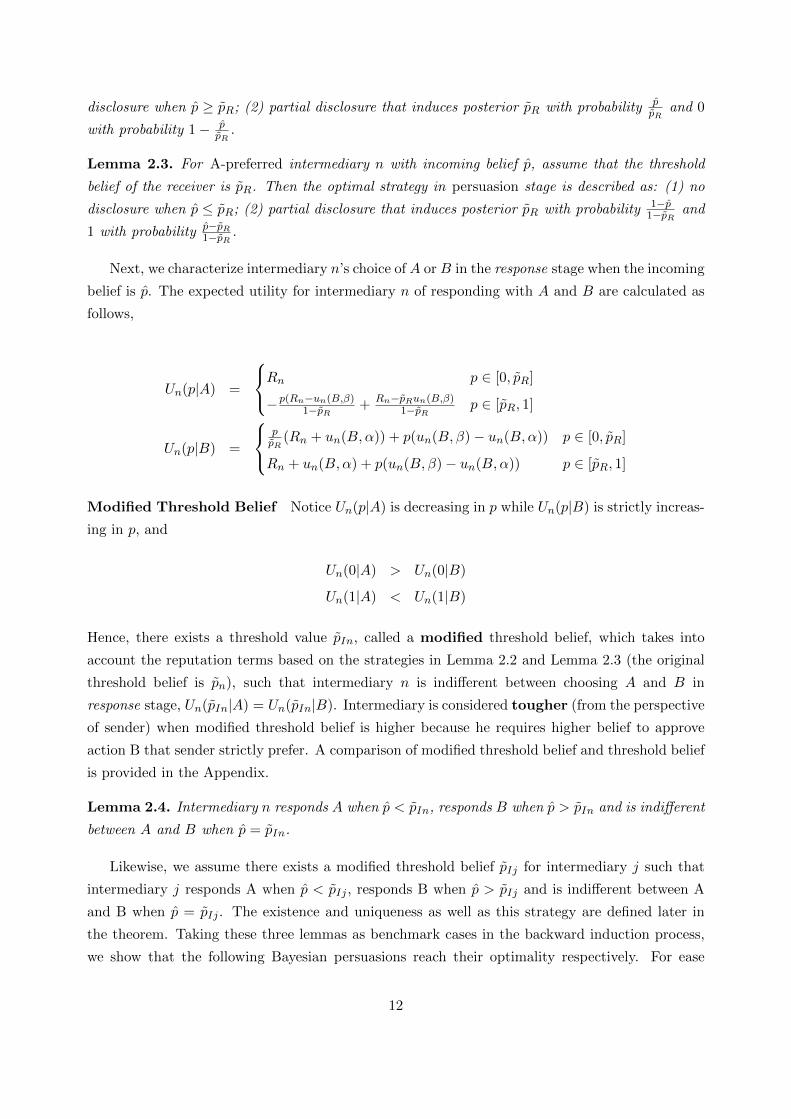
Timeline of the Game Each intermediary participates in two stages, a response stage in

which intermediaries reply to the preceding intermediary to report their intended message, and

a persuasion stage in which that intermediary persuades the succeeding intermediary. Note that

as the initial and terminal notes of the hierarchy, the sender only has a persuasion stage while

the receiver only has a response stage. In the response stage, an intermediary chooses a reply

2In our example, the professors, committee chairs, and final admissions decision-maker prefer to admit the studentif and only if he is a good scholar.

3For example, either the faculty letter writer or the admissions chair may incur a higher disutility if a goodstudent is rejected, or if a bad student is admitted to the program.

4For example, a professor may tell a student that he is happy to write the student a good letter of recommendation.A faculty level admissions chair may tell the department level admissions chair that he will forward the departmentlevel admission suggestion to the next level of evaluation.

5Without this reputation concern, the model will reduce to one in which all intermediaries are truth-telling inequilibrium, in the sense of simply passing forward the information received along the hierarchy.

8

from D = {A,B} after the preceding intermediary implementing his persuasion strategy. Figure

1 illustrates the timing of response and persuasion stages. The black dashed rectangle represents

a specific meeting in which player j attempts to persuade player j + 1 and player j + 1 responds

to player j.

Response Stage

Persuasion Stage

Sender

Intermediary 1

represents

represents

Receiver

Intermediary 2

……

Intermediary n-1

Intermediary n

……

……

……

Figure 1: Stages of the Game

1. Commitment Process

We follow in the commitment feature of the original model by Kamenica and Gentzkow

(2011). In their framework, the sender’s persuasion strategy is a commitment to a distri-

bution of signals, conditional on the true state of the world. In the hierarchical setting,

the sender has such a persuasion strategy, while the intermediaries commit to a distribution

of signals conditional on both state and their signal received from the sender or previous

intermediaries.

We can think of this commitment to a conditional distribution as a type of formal policy

which is made known to the other players in the game. For example, in the academic

recommendation case, a professor may adopt a policy to only provide a strong to very strong

recommendation letter to a student who has met certain qualifications, such as specific

coursework and research experience. A department admissions committee chair may have a

policy to highly recommend a student for admission at the faculty level if the student has

obtained certain grade point average and test score levels. In a hierarchical setting which

9

has some elements of a bureaucracy, it may be reasonable in particular, for intermediaries

to make such policies or commitment strategies.

• The sender publicly sets up a signal-generating mechanism, which consists of a family

of conditional distributions {π(·|t)}t∈T over a space of signal realizations S6 and hence

divides the prior belief into posterior portfolios that satisfy a Bayes plausible condition.

We refer to this as a belief division process.

• Intermediary 1 publicly sets a response rule7 as well as a signal-generating mechanism

which consists of a family of conditional distributions {π(·|s, t)}s∈S,t∈T over a space

of signal realizations I1 on Cartesian product of signal received from the immediately

preceding player (the sender) and the state8, and hence divides his incoming belief

conditioning on s into posterior portfolios that satisfies the Bayes plausible condition

as well. Then sequentially and publicly, intermediaries j = 2, · · · , n, announce their

response rules and belief division processes9.

2. Realization Process

With these strategies in place by each player in the game, the state is realized and the course

of events is as follows

• Nature determines the true state t, which is privately observed by the sender.

• According to the commitment strategies established, the signals are then generated one

by one, each of which is privately10 observed only by the next intermediary.

• According to the commitment strategies established, the replies of each player for their

response stage are implemented, and observed only by the immediately preceding player.

• After observing intermediary n’s signal realization, the receiver chooses an action from

{A,B}.

Note that in contrast to non-hierarchical persuasion-game models, the sender in our framework

does not have direct control over what the intermediaries and receiver might observe; instead, she

tries to influence the receivers’ decision by setting up a signal-generating mechanism. This can also

be interpreted in our academic setting as a revelation of academic performance measures, research

progress, and so on, after the student establishes a study plan. The ex-ante mechanism being used

for obtaining the signal, and the realized evidence that emerges are then communicated to the

6Sender publicly designs a mapping T → ∆S.7Decide when responds A and when responds B8Intermediary 1 publicly designs a mapping T × S → ∆I1.9Intermediary j publicly designs a mapping T × Ij−1 → ∆Ij .

10Because the posterior distribution can be uniquely derived from signal realization ij−1 received from intermediaryj − 1 for intermediary j.

10

next decision-maker in the chain without noise. A similar process is true for each intermediary in

the chain.11

The game is sequential in nature, in that each player’s commitment strategy for the persuasion

and response stages is set in sequence, after observing the commitment strategy of the previous

player in the hierarchy. Once these strategies are set, the true state is realized, and the realization

of the strategies are implemented automatically (with the assistance of a randomization device to

implement stochastic elements of strategies).

2.2 Equilibrium Analysis

With the setup of the game established, we now analyze the equilbria of the game. The solution

concept is essentially subgame perfect Nash equilibrium, as the game is sequential while no player

has private information at the point in the game when strategies are determined.12

We refer to an intermediary as A-preferred if he chooses A in the response stage. We refer to

an intermediary as B-preferred if he chooses B in the response stage. We first characterize the

condition that players’ optimal strategy in persuasion stage is indeed maximizing the likelihood

of his preferred action being chosen by the receiver. The following statement provides a sufficient

condition.

Assumption 2.1. An intermediary j’s reputation gain has a lower bound,

Rj > max(− uj(B,α), uj(B, β)

)(1)

We assume that any intermediary’s reputation gain is greater than their own utility gain

(or loss) in either true state, should the eventual decision be B. It is reasonable to think that

intermediaries usually care more about their reputation compared with sender and receiver who

in our framework only care about the final decision. Please refer to appendix for the discussion of

the role of the reputation term.

We use backward induction to characterize the optimal Bayesian persuasion. By Kamenica

and Gentzkow (2011) [1], the following two lemmas hold with regard to the final intermediary n. In

following sections, we use p̂ to denote incoming belief that Bayesian updated from signal realization

of preceding player.

Lemma 2.2. For B-preferred intermediary n with incoming belief p̂, assume that the threshold

belief of the receiver is p̃R. Then the optimal strategy in persuasion stage is described as: (1) no

11In the case of an intermediary, such as the faculty letter writer, an ex-ante stochastic policy is set and madeknown to all players. Based on the signal received from the student, the letter writer’s preset stochastic policy isimplemented. In a real world setting, such stochastic policy could involve a strong to very strong, or mediocre tomoderately strong letter. However in our simplified setting, the only actions available to the faculty member are notrecommend (A) or recommend (B), which means that in the current setting, a non-degenerate stochastic policy willhave each of not recommend or recommend being conveyed to the next intermediary with positive probability.

12This follows Kamenica and Gentzkow (2011), where note that once nature determines the true state, the stateis private information to the sender. However at this point in the game, the strategies are already set by all players.

11

disclosure when p̂ ≥ p̃R; (2) partial disclosure that induces posterior p̃R with probability p̂p̃R

and 0

with probability 1− p̂p̃R

.

Lemma 2.3. For A-preferred intermediary n with incoming belief p̂, assume that the threshold

belief of the receiver is p̃R. Then the optimal strategy in persuasion stage is described as: (1) no

disclosure when p̂ ≤ p̃R; (2) partial disclosure that induces posterior p̃R with probability 1−p̂1−p̃R and

1 with probability p̂−p̃R1−p̃R .

Next, we characterize intermediary n’s choice of A or B in the response stage when the incoming

belief is p̂. The expected utility for intermediary n of responding with A and B are calculated as

follows,

Un(p|A) =

Rn p ∈ [0, p̃R]

−p(Rn−un(B,β)1−p̃R + Rn−p̃Run(B,β)

1−p̃R p ∈ [p̃R, 1]

Un(p|B) =

pp̃R

(Rn + un(B,α)) + p(un(B, β)− un(B,α)) p ∈ [0, p̃R]

Rn + un(B,α) + p(un(B, β)− un(B,α)) p ∈ [p̃R, 1]

Modified Threshold Belief Notice Un(p|A) is decreasing in p while Un(p|B) is strictly increas-

ing in p, and

Un(0|A) > Un(0|B)

Un(1|A) < Un(1|B)

Hence, there exists a threshold value p̃In, called a modified threshold belief, which takes into

account the reputation terms based on the strategies in Lemma 2.2 and Lemma 2.3 (the original

threshold belief is p̃n), such that intermediary n is indifferent between choosing A and B in

response stage, Un(p̃In|A) = Un(p̃In|B). Intermediary is considered tougher (from the perspective

of sender) when modified threshold belief is higher because he requires higher belief to approve

action B that sender strictly prefer. A comparison of modified threshold belief and threshold belief

is provided in the Appendix.

Lemma 2.4. Intermediary n responds A when p̂ < p̃In, responds B when p̂ > p̃In and is indifferent

between A and B when p̂ = p̃In.

Likewise, we assume there exists a modified threshold belief p̃Ij for intermediary j such that

intermediary j responds A when p̂ < p̃Ij , responds B when p̂ > p̃Ij and is indifferent between A

and B when p̂ = p̃Ij . The existence and uniqueness as well as this strategy are defined later in

the theorem. Taking these three lemmas as benchmark cases in the backward induction process,

we show that the following Bayesian persuasions reach their optimality respectively. For ease

12

of notation, we denote the sender as intermediary 0. The following Theorem characterizes one

optimal signal and the associated sub-game perfect equilibrium, as an induction case. Before

that, for any intermediary j we define the maximum modified threshold belief of all successors

(intermediaries j + 1, · · · , n and the receiver) as p̃maxj = max

({p̃Ik}nk=j+1, p̃R

); the minimum

modified threshold belief of all successors (intermediaries j + 1, · · · , n and the receiver) is defined

as p̃minj = min

({p̃Ik}nk=j+1, p̃R

). Notice here the subscript of p̃min

j and p̃maxj is j rather than Ij

for convenience.

In the following equilibrium, only the sender alters the information structure, which we refer

to as a one-step equilibrium. The induction process is concluded in Figure 2.

Inp

nn-1… Rn-2

Strategy ofB preferred

Strategy ofA preferred

max

np

min

np

Rp, 1I np

Strategy ofB preferred

Strategy ofA preferred

max

1np

min

1np

, 2I np

Strategy ofB preferred

Strategy ofA preferred

max

2np

min

2np

j

, 2I np

Strategy ofB preferred

Strategy ofA preferred

max

2np

min

2np

Figure 2: Induction Process of Equilibrium

Theorem 2.5 (One-step Equilibrium).

1. In the persuasion stage,

• For B-preferred intermediary j with incoming belief p̂, the following Bayesian persua-

sion process is optimal: (1) no disclosure when p̂ ≥ p̃maxj ; (2) partial disclosure that

induces posterior p̃maxj with probability p̂

p̃maxj

and 0 with probability 1− p̂p̃maxj

.

• For A-preferred intermediary j with incoming belief p̂, the following Bayesian persua-

sion process is optimal: (1) no disclosure when p̂ ≤ p̃minj ; (2) partial disclosure that

induces posterior p̃minj with probability 1−p̂

1−p̃minj

and 1 with probabilityp̂−p̃min

j

1−p̃minj

.

13

2. In response stage,

• Intermediary j responds A when p̂ < p̃Ij, responds B when p̂ > p̃Ij and is indifferent

between A and B when p̂ = p̃Ij, where p̃Ij is defined by

Uj(p̃Ij |A) = Uj(p̃Ij |B) (2)

where

Uj(p|A) =

Rj p ∈ [0, p̃minj ]

1−p1−p̃min

jRj +

p−p̃minj

1−p̃minjuj(B, β) p ∈ [p̃min

j , 1]

Uj(p|B) =

p

p̃maxj

(Rj + uj(B,α)) + p(uj(B, β)− uj(B,α)) p ∈ [0, p̃maxj ]

Rj + uj(B,α) + p(uj(B, β)− uj(B,α)) p ∈ [p̃maxj , 1]

Proof of Theorem 2.5:

1. Persuasion Stage

When j = n, the results in the Theorem hold according to Lemma 2.2, Lemma 2.3, and

Lemma 2.4. Assume that for j = k + 1, · · · , n, the results in the theorem hold. We then prove

that for j = k, the results in the theorem hold.

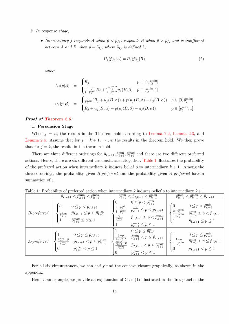
There are three different orderings for p̃I,k+1, p̃mink+1, p̃

maxk+1 and there are two different preferred

actions. Hence, there are six different circumstances altogether. Table 1 illustrates the probability

of the preferred action when intermediary k induces belief p to intermediary k + 1. Among the

three orderings, the probability given B-preferred and the probability given A-preferred have a

summation of 1.

Table 1: Probability of preferred action when intermediary k induces belief p to intermediary k+1p̃I,k+1 < p̃min

k+1 < p̃maxk+1 p̃min

k+1 < p̃I,k+1 < p̃maxk+1 p̃min

k+1 < p̃maxk+1 < p̃I,k+1

B-preferred

0 0 ≤ p < p̃I,k+1p

p̃maxk+1

p̃I,k+1 ≤ p < p̃maxk+1

1 p̃maxk+1 ≤ p ≤ 1

0 0 ≤ p < p̃mink+1

p−p̃minj

1−p̃minj

p̃mink+1 ≤ p < p̃I,k+1

pp̃maxk+1

p̃I,k+1 ≤ p < p̃maxk+1

1 p̃maxk+1 ≤ p ≤ 1

0 0 ≤ p < p̃min

k+1p−p̃min

j

1−p̃minj

p̃mink+1 ≤ p < p̃I,k+1

1 p̃I,k+1 ≤ p ≤ 1

A-preferred

1 0 ≤ p ≤ p̃I,k+1p̃maxk+1−pp̃maxk+1

p̃I,k+1 < p ≤ p̃maxk+1

0 p̃maxk+1 < p ≤ 1

1 0 ≤ p ≤ p̃mink+1

1−p1−p̃min

jp̃mink+1 < p ≤ p̃I,k+1

p̃maxk+1−pp̃maxk+1

p̃I,k+1 < p ≤ p̃maxk+1

0 p̃maxk+1 < p ≤ 1

1 0 ≤ p ≤ p̃min

k+11−p

1−p̃minj

p̃mink+1 < p ≤ p̃I,k+1

0 p̃I,k+1 < p ≤ 1

For all six circumstances, we can easily find the concave closure graphically, as shown in the

appendix.

Here as an example, we provide an explanation of Case (1) illustrated in the first panel of the

14

associated appendix. For other cases illustrated in other panels, we omit the detailed reasoning

which is analogous to that of Case (1).

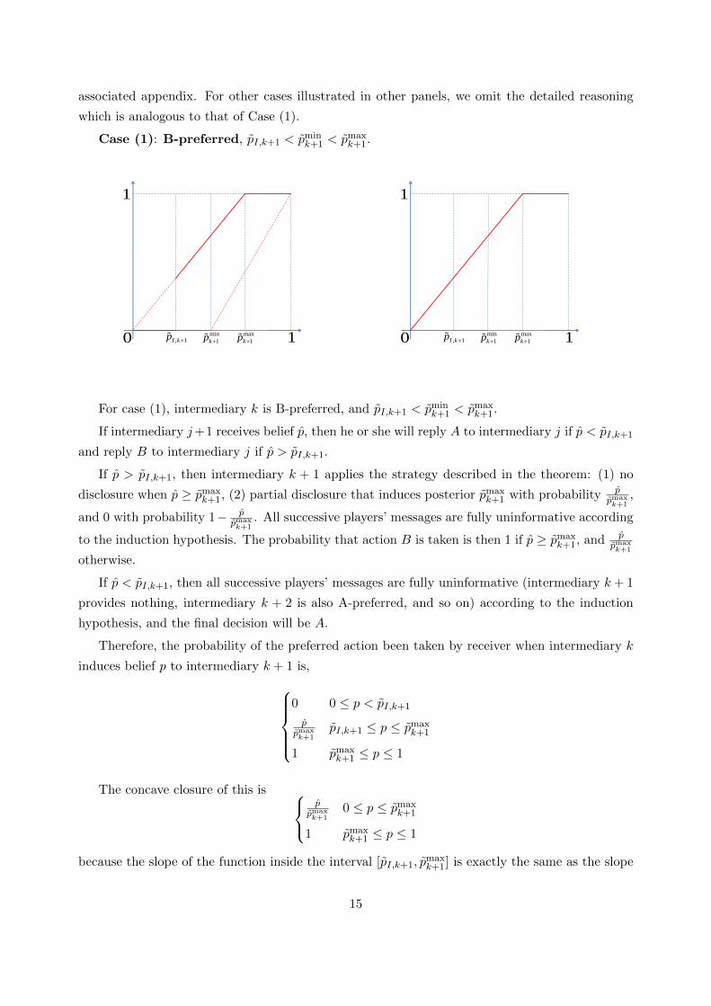
Case (1): B-preferred, p̃I,k+1 < p̃mink+1 < p̃max

k+1.

max

1kp

1

10 min

1kp , 1I kp

max

1kp

1

10 min

1kp , 1I kp

For case (1), intermediary k is B-preferred, and p̃I,k+1 < p̃mink+1 < p̃max

k+1.

If intermediary j+1 receives belief p̂, then he or she will reply A to intermediary j if p̂ < p̃I,k+1

and reply B to intermediary j if p̂ > p̃I,k+1.

If p̂ > p̃I,k+1, then intermediary k + 1 applies the strategy described in the theorem: (1) no

disclosure when p̂ ≥ p̃maxk+1, (2) partial disclosure that induces posterior p̃max

k+1 with probability p̂p̃maxk+1

,

and 0 with probability 1− p̂p̃maxk+1

. All successive players’ messages are fully uninformative according

to the induction hypothesis. The probability that action B is taken is then 1 if p̂ ≥ p̃maxk+1, and p̂

p̃maxk+1

otherwise.

If p̂ < p̃I,k+1, then all successive players’ messages are fully uninformative (intermediary k + 1

provides nothing, intermediary k + 2 is also A-preferred, and so on) according to the induction

hypothesis, and the final decision will be A.

Therefore, the probability of the preferred action been taken by receiver when intermediary k

induces belief p to intermediary k + 1 is,0 0 ≤ p < p̃I,k+1

p̂p̃maxk+1

p̃I,k+1 ≤ p ≤ p̃maxk+1

1 p̃maxk+1 ≤ p ≤ 1

The concave closure of this is p̂

p̃maxk+1

0 ≤ p ≤ p̃maxk+1

1 p̃maxk+1 ≤ p ≤ 1

because the slope of the function inside the interval [p̃I,k+1, p̃maxk+1] is exactly the same as the slope

15

of the line connecting the origin point to (p̃I,k+1,p̃I,k+1

p̃maxk+1

).

Since p̃max and p̃min have the following iterative relationships,

p̃maxk =

p̃maxk+1 p̃I,k+1 < p̃max

k+1

p̃I,k+1 p̃I,k+1 > p̃maxk+1

(3)

p̃mink =

p̃I,k+1 p̃I,k+1 < p̃mink+1

p̃mink+1 p̃I,k+1 > p̃min

k+1

(4)

Therefore, when j = k, the result regarding the persuasion stage in the Theorem holds.

2. Response Stage

The expected utilities for intermediary k by responding with A and B are calculated respec-

tively as follow,

Uk(p|A) =

Rk p ∈ [0, p̃mink ]

1−p1−p̃min

k

Rk +p−p̃min

k

1−p̃mink

uk(B, β) p ∈ [p̃mink , 1]

Uk(p|B) =

p

p̃maxk

(Rk + uk(B,α)) + p(uk(B, β)− uk(B,α)) p ∈ [0, p̃maxk ]

Rk + uk(B,α) + p(uk(B, β)− uk(B,α)) p ∈ [p̃maxk , 1]

Since Uk(p|A) is decreasing in p while Uk(p|B) is strictly increasing in p, and

Uk(0|A) > 0

Uk(1|A) < Uk(1|B)

there exists a modified threshold belief p̃Ik such that intermediary k is indifferent between choosing

A and B in response stage, Uk(p̃Ik|A) = Uk(p̃Ij |B). Therefore, our theorem holds when j = k,

which completes our proof.

The above optimal Bayesian persuasion gives us the following equilibrium strategy of the

sender, (1) no disclosure when p0 ≥ p̃max0 ; (2) partial disclosure that induces posterior p̃max

0 with

probability p0p̃max0

and 0 with probability 1 − p0p̃max0

. Since we denote the sender as intermediary 0,

p̃max0 is defined as the maximum of all modified threshold beliefs of intermediary and threshold

hold belief of receiver. No intermediary alters the information structure released by the sender.

In addition, instead of using uj(B,α), uj(B, β), Rj , the modified threshold beliefs of the players

are sufficient for characterization of equilibrium. We call the intermediary with highest modified

threshold toughest intermediary. If modified threshold belief of toughest player is higher than

p̃R, we can this intermediary the toughest player; otherwise, we call receiver the toughest player.

The following corollary summarizes the features of the persuasion equilibrium.

16

Corollary 2.6. In the one-step Bayesian persuasion equilibrium,

1. Bayesian persuasion is only determined by p̃max0 .

• Hierarchical Bayesian persuasion is outcome equivalent to persuading the toughest player

(among intermediaries and receiver) directly13;Note to Jaimie/Jie: Actually it is not

equivalent to persuade the toughest player only. The parameters of succeeding players

will influence the modified threshold beliefs. Hence, I change to directly, which means

we can drop all players in front of toughest player.

• When belief p̃max0 is induced, all players prefer action B, and B is chosen;

• When belief 0 is induced, intermediaries and the receiver prefer action A, and A is

chosen.

2. Each intermediary provides no additional information and merely transmits the message that

previous intermediaries do.

Clearly, the analysis has not characterized all equivalent possible optimal Bayesian persuasions.

The literature is mainly concerned about the payoff or welfare benefits of Bayesian persuasion

compared with degenerate strategies (such as no disclosure and full disclosure) rather than focusing

on fully characterizing all possible equilibria.

In the prosecutor-judge case illustrated in Kamenica and Gentzkow (2011), when the prior

probability of guilt is 0.7, it is also optimal to induce posteriors 0.6 and 0.8 with equal probability.

In our setting, when incoming belief p̂ is lower than p̃I,k+1, one may choose partial disclosure that

induces any posterior p ∈ [p̃I,k+1, p̃maxk+1] with probability p̂

p and 0 with probability 1 − p̂p when

p̂ < p̃maxk+1.

Nonetheless, there exists another intuitive optimal Bayesian persuasion which we call myopic

equilibrium. In the one-step equilibrium, only the sender manipulates the information structure

and intermediaries provide no additional information, merely transmitting what the previous inter-

mediary does. Compared with this structure, in the myopic equilibrium, each player only aims to

persuade the immediately subsequent player. In this case, some intermediaries provide a different

signal structure, which depends on how difficult it is to persuade the subsequent intermediary.

Theorem 2.7 (Myopic Equilibrium).

1. In the persuasion stage,

• For B-preferred intermediary j with incoming belief p̂, the following Bayesian persua-

sion process is optimal: (1) no disclosure when p̂ ≥ p̃I,j+1; (2) partial disclosure that

induces posterior p̃I,j+1 with probability p̂p̃I,j+1

and 0 with probability 1− p̂p̃I,j+1

.

13Then all succeeding players will merely pass the information.

17

• For A-preferred intermediary j with incoming belief p̂, the following Bayesian persua-

sion process is optimal: (1) no disclosure when p̂ ≤ p̃I,j+1; (2) partial disclosure that

induces posterior p̃I,j+1 with probability 1−p̂1−p̃I,j+1

and 1 with probabilityp̂−p̃I,j+1

1−p̃I,j+1.

2. In the response stage,

• Intermediary j responds A when p̂ < p̃Ij, responds B when p̂ > p̃Ij and is indifferent

between A and B when p̂ = p̃Ij, where p̃Ij is defined by

Uj(p̃Ij |A) = Uj(p̃Ij |B) (5)

The difference in the myopic equilibrium compared to the one-step equilibrium is that suc-

ceeding players may provide additional information. However, the two possible posteriors received

by receiver are still 0, p̃max0 , identical to the case of the one-step equilibrium. When p̂ > p̃I,k+1,

the probability that action B is taken is 1 if p̂ ≥ p̃maxk+1, and p̂

p̃maxk+1

otherwise. The outcome and

associated payoffs of the game are unchanged.

The proof is analogous to that for the one-step equilibrium. However, in this equilibrium, the

information transmission process is quite different. We say that intermediary y is the next node

after intermediary x, written as x → y, if she is the nearest subsequent intermediary that has a

higher modified threshold belief p̃Iy > p̃Ix. Mathematically, x→ y if and only if,

y > x, p̃Iy > p̃Ix and ∀x < z < y, p̃Iz ≤ p̃Ix

We say intermediaries c0, c1, · · · , cm form an increasing chain if and only if ci → ci+1, ∀j =

0, · · · ,m− 1. Hence, for the n intermediaries and the receiver, we can find the unique increasing

chain starting from intermediary 1 (as the first node). We assume that this unique increasing

chain is 1 → i1 → · · · → im. 14 The above optimal Bayesian persuasion gives us the following

equilibrium strategy of players: no disclosure (in other words, simply pass along the message

received) if the next intermediary is not in increasing chain; otherwise, (1) when incoming belief is

p̃I,ij−1 , partial disclosure that induces posterior p̃I,ij with probabilityp̃I,ij−1

p̃I,ijand 0 with probability

p̃I,ij−1

p̃I,ij; (2) when incoming belief is 0, no disclosure.

2.3 Shortsighted Players

The results of the previous analysis only depend on the modified threshold beliefs of players

and the equilibrium analysis is based on the following standard assumptions,

• The game theoretic rationality of all players are common knowledge.

• The parameters of all players are common knowledge.

14Intermediary im may be the receiver.

18

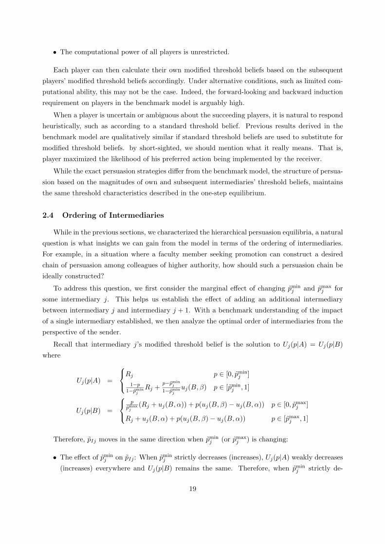
• The computational power of all players is unrestricted.

Each player can then calculate their own modified threshold beliefs based on the subsequent

players’ modified threshold beliefs accordingly. Under alternative conditions, such as limited com-

putational ability, this may not be the case. Indeed, the forward-looking and backward induction

requirement on players in the benchmark model is arguably high.

When a player is uncertain or ambiguous about the succeeding players, it is natural to respond

heuristically, such as according to a standard threshold belief. Previous results derived in the

benchmark model are qualitatively similar if standard threshold beliefs are used to substitute for

modified threshold beliefs. by short-sighted, we should mention what it really means. That is,

player maximized the likelihood of his preferred action being implemented by the receiver.

While the exact persuasion strategies differ from the benchmark model, the structure of persua-

sion based on the magnitudes of own and subsequent intermediaries’ threshold beliefs, maintains

the same threshold characteristics described in the one-step equilibrium.

2.4 Ordering of Intermediaries

While in the previous sections, we characterized the hierarchical persuasion equilibria, a natural

question is what insights we can gain from the model in terms of the ordering of intermediaries.

For example, in a situation where a faculty member seeking promotion can construct a desired

chain of persuasion among colleagues of higher authority, how should such a persuasion chain be

ideally constructed?

To address this question, we first consider the marginal effect of changing p̃minj and p̃max

j for

some intermediary j. This helps us establish the effect of adding an additional intermediary

between intermediary j and intermediary j + 1. With a benchmark understanding of the impact

of a single intermediary established, we then analyze the optimal order of intermediaries from the

perspective of the sender.

Recall that intermediary j’s modified threshold belief is the solution to Uj(p|A) = Uj(p|B)

where

Uj(p|A) =

Rj p ∈ [0, p̃minj ]

1−p1−p̃min

jRj +

p−p̃minj

1−p̃minjuj(B, β) p ∈ [p̃min

j , 1]

Uj(p|B) =

p

p̃maxj

(Rj + uj(B,α)) + p(uj(B, β)− uj(B,α)) p ∈ [0, p̃maxj ]

Rj + uj(B,α) + p(uj(B, β)− uj(B,α)) p ∈ [p̃maxj , 1]

Therefore, p̃Ij moves in the same direction when p̃minj (or p̃max

j ) is changing:

• The effect of p̃minj on p̃Ij : When p̃min

j strictly decreases (increases), Uj(p|A) weakly decreases

(increases) everywhere and Uj(p|B) remains the same. Therefore, when p̃minj strictly de-

19

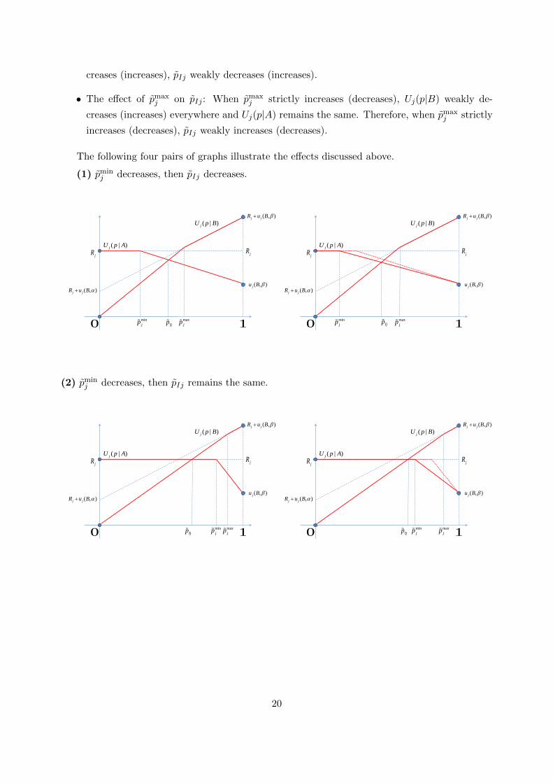
creases (increases), p̃Ij weakly decreases (increases).

• The effect of p̃maxj on p̃Ij : When p̃max

j strictly increases (decreases), Uj(p|B) weakly de-

creases (increases) everywhere and Uj(p|A) remains the same. Therefore, when p̃maxj strictly

increases (decreases), p̃Ij weakly increases (decreases).

The following four pairs of graphs illustrate the effects discussed above.

(1) p̃minj decreases, then p̃Ij decreases.

0 1

jR

( , )j jR u B

( , )j jR u B

( , )ju B

jR

max

jpmin

jpIjp

( | )jU p A

( | )jU p B

0 1

jR

( , )j jR u B

( , )j jR u B

( , )ju B

jR

max

jpmin

jp Ijp

( | )jU p A

( | )jU p B

(2) p̃minj decreases, then p̃Ij remains the same.

0 1

jR

( , )j jR u B

( , )j jR u B

( , )ju B

jR

max

jpmin

jpIjp

( | )jU p A

( | )jU p B

0 1

jR

( , )j jR u B

( , )j jR u B

( , )ju B

jR

max

jpmin

jpIjp

( | )jU p A

( | )jU p B

20

(3) p̃maxj decreases, then p̃Ij decreases.

0 1

jR

( , )j jR u B

( , )j jR u B

( , )ju B

jR

max

jpmin

jpIjp

( | )jU p A

( | )jU p B

0 1

jR

( , )j jR u B

( , )j jR u B

( , )ju B

jR

max

jpmin

jpIjp

( | )jU p A

( | )jU p B

(4) p̃maxj decreases, then p̃Ij remains the same.

0 1

jR

( , )j jR u B

( , )j jR u B

( , )ju B

jR

max

jpmin

jpIjp

( | )jU p A

( | )jU p B

0 1

jR

( , )j jR u B

( , )j jR u B

( , )ju B

jR

max

jpmin

jpIjp

( | )jU p A

( | )jU p B

2.4.1 Adding an intermediary j′ between j and j + 1

When we add another intermediary (labeled j′) after an intermediary j and in front of inter-

mediary j + 1, then we can solve for the modified threshold belief of this new intermediary.

If this new modified threshold belief lies within the range [p̃minj , p̃max

j ], then nothing will change.

If this new modified threshold belief is less than p̃minj , then the modified threshold belief of inter-

mediary j weakly decreases. This decrease may lead p̃minj−1 to decrease, p̃max

j−1 to decrease, both, or

none. Under each of those four circumstances, p̃I,j−1 weakly decreases. Recursively, the modified

threshold beliefs of all intermediaries before j weakly decrease.

If this new modified threshold belief is larger than p̃maxj , then the modified threshold belief

21

of intermediary j weakly increases. This decrease may have the effect that either p̃minj−1 increases,

p̃maxj−1 increases, both, or none. Under each of those four circumstances, p̃I,j−1 weakly increases.

Recursively, the modified threshold beliefs of all intermediaries before j weakly increase.

In the benchmark model, direct communication with the receiver is weakly better than indirect

communication with the receiver. However, the generalization of this statement to endogenously

chosen intermediaries is not true. More people involved in the persuasion process will not nec-

essarily make the sender worse off. In particular, adding one ”nice” intermediary (who is easier

to convince) can decrease the p̃max0 for the sender, and hence increase the probability of desirable

action B.

Corollary 2.8. Adding an intermediary can decrease p̃max0 in equilibrium.

Example 2.9. Prior probability p0 = 13 .

• Receiver has threshold belief p̃R = 0.5.

• Player J has parameter uJ(B,α) = −3, uJ(B, β) = 1 and reputation RJ = 4.

• Player K has parameter uK(B,α) = −1, uK(B, β) = 3 and reputation RK = 4.

If player J is the unique intermediary, then the modified threshold belief of player J is 23 .

Hence, the probability that action B is taken is 12 in the optimal Bayesian persuasion.

If player K is added between player J and the receiver, then the modified threshold belief of

player K is 25 and the modified threshold belief of player J is reduced to 5

9 . Hence, the probability

that action B is taken is 35 in the optimal Bayesian persuasion.

The receiver makes his decision solely based on type-dependent utility. However, the inter-

mediaries care about their reputations. The influence of the reputation term depends on each

intermediary’s anticipation of the subsequent players. Adding one easy to convince intermediary

after the toughest intermediary may decrease p̃minj , and hence decrease utility of the toughest in-

termediary when responding to the previous player with undesirable action A. By our analysis on

the effect of p̃minj on p̃Ij , the modified threshold belief of the toughest player may decrease.

2.4.2 The Sender’s optimal order

With the previous results established, we now assume that the parameters of the intermediaries

are given, and the sender can pre-arrange the order of intermediaries. Which permutation of

intermediaries is ideal from the sender’s perspective? From the analysis in the benchmark model,

we know that the sender seeks to minimize p̃max0 , where for ease of notation we denote the sender

as intermediary 0.

We assume that there are n intermediaries, with parameters {RJ , uJ(B, β), uJ(B,α)}J=1,2,··· ,n.

We use the capital letter subscript J to represent the labeling of different players, distinguished

from small letter subscript j which represents a player’s position in the hierarchy.

22

Then an order is a permutation σ defining a one-to-one mapping from {1, 2, · · · , n} to itself.

σ(J) = j means that player J is located at position j.

For further analysis, for player J , we define the degree of sender-alignment using the following

formula,

KJ =(RJ + uJ(B,α)

p̃R+ uJ(B, β)− uJ(B,α)

)R−1J > 1 (6)

The higher the value, the more aligned the interests of the intermediary are with the sender.15

The player with highest degree of sender-alignment is called the most sender-aligned intermediary.

The intermediary favors action B more if uJ(B,α) or uJ(B, β) increases. When uJ(B, β) or

uJ(B,α) (or both) increases, KJ will increase and hence he becomes a more sender-aligned player.

For further analysis, we define the inverse degree of sender-alignment as,

pJ

= K−1J = RJ

(RJ + uJ(B,α)

p̃R+ uJ(B, β)− uJ(B,α)

)−1(7)

which is a probability measure such that pJ∈ (0, 1).

Observation 2.10. • pJ

= p̃R if and only if p̃J = p̃R.

• pJ> p̃R if and only if p̃J > p̃R

• pJ< p̃R if and only if p̃J < p̃R

where p̃J denotes the threshold belief of player J .

We first obtain a lower bound on p̃min0 . Sometimes, p̃min

0 = p̃R, which means that the receiver

is actually the most sender-aligned player in the hierarchy. If not, we can see that p̃min0 is bounded

by the inverse degree of sender-alignment.

Lemma 2.11. If for some permutation, p̃min0 < p̃R, then

p̃min0 ≥ min

JpJ

= (maxJ

KJ)−1 (8)

Proof. Assume that p̃min0 is attained for player K located at position k, p̃min

0 = p̃Ik. Then p̃Ik is

defined by the intersection point of Uk(p|A) and Uk(p|B). Since we must have p̃Ik ≤ p̃mink ≤ p̃max

k ,

then p̃Ik solves

RK =p

p̃maxk

(RK + uK(B,α)) + p(uK(B, β)− uK(B,α)) (9)

where the left hand side is the expression of Uk(p|A) when p ≤ p̃mink , and the right hand side is

the expression of Uk(p|B) when p ≤ p̃maxk . Then by the fact that p̃max

k ≥ p̃R, we have the following

relationship,

RK ≤p

p̃R(RK + uK(B,α)) + p(uK(B, β)− uK(B,α)) (10)

15KJ > 1 because RJ+uJ (B,α)p̃R

+uJ(B, β)−uJ(B,α) ≥ RJ +uJ(B,α)+uJ(B, β)−uJ(B,α) = RJ +uJ(B, β) > RJ

23

after rearranging, we obtain

p̃Ik ≥ RK(RK + uK(B,α)

p̃R+ uK(B, β)− uK(B,α)

)= p

K≥ min

JpJ

We then claim that such lower bound can be attained under some specific permutations, in

which the most sender-aligned intermediary talks to the receiver directly.

Lemma 2.12. If it is true that (1) there exists some permutation such that p̃min0 < p̃R, (2)

K = arg minJ pJ , then for all permutations σ such that σ(K) = n, we have

p̃min0 = min

JpJ

= pK

(11)

Proof. We can verify that p̃In = pK

solves Un(p|A) = Un(p|B) and p̃In < p̃R = p̃minn = p̃max

n . Then

p̃min0 ≤ p̃In because p̃min

0 is the minimum among all modified threshold beliefs. According to the

previous lemma, we can conclude that p̃min0 = minJ pJ .

Both Lemma 2.11 and Lemma 2.12 require the condition that there exists some permutation

such that p̃min0 < p̃R. However, when does such a permutation exist? The following lemma shows

us that such permutation exists if and only if minJ pJ < p̃R. If this condition is met, we call the

most sender-aligned intermediary the most sender-aligned player. If this relationship is not met, we

call receiver the most sender-aligned player. Recall from Observation 2.10, that the minJ pJ < p̃R

condition is equivalent to the existence of at least one player with threshold belief smaller than

p̃R, which provides us with an easier determination rule, regardless of whether we can obtain

p̃min0 < p̃R.16 To summarize,

minJpJ< p̃R ⇐⇒ min

Jp̃J < p̃R

Lemma 2.13. • If minJ pJ < p̃R and K = arg minJ pJ , then for all permutations σ such that

σ(K) = n, we have

p̃min0 = min

JpJ

(12)

• If minJ pJ ≥ p̃R, under all permutations σ, p̃min0 = p̃R.

Proof. If minJ pJ < p̃R, and K = arg minJ pJ , by ordering player K as intermediary n, we can

get a threshold belief p̃In = pK< p̃R. Then, condition (1) of the previous lemma is satisfied, and

hence p̃min0 = minJ pJ .

If minJ pJ ≥ p̃R, we need to show that under all permutations, the modified threshold belief of

all intermediaries cannot be less than p̃R, which is equivalent to proving that Uj(p̃R|B) ≤ Uj(p̃R|A)

for all intermediaries j. We can prove this by induction. For intermediary n, we have the following

equivalent inequalities,

16Note however, that pJ

and p̃J may not be minimized by the same J .

24

Rn(Rn + un(B,α)

p̃R+ un(B, β)− un(B,α)

)−1 ≥ p̃R

p̃R(Rn + un(B,α)

p̃R+ un(B, β)− un(B,α)

)≤ Rn

Un(p̃R|B) = Rn + un(B,α) + p̃R(un(B, β)− un(B,α)) ≤ Rn = Un(p̃R|A)

Assume that for intermediary j, p̃minj = p̃R, we have the following equivalent inequalities,

Rj(Rj + uj(B,α)

p̃R+ uj(B, β)− uj(B,α)

)−1 ≥ p̃R

p̃R(Rj + uj(B,α)

p̃R+ uj(B, β)− uj(B,α)

)≤ Rj

Rj + uj(B,α) + p̃R(uj(B, β)− uj(B,α)) ≤ Rj

Multiplying the Rj +uj(B,α) term by a constant p̃Rp̃maxj

that is less than or equal to 1, the left hand

side is reduced to,

Uj(p̃R|B) =p̃Rp̃maxj

(Rj + uj(B,α)) + p̃R(uj(B, β)− uj(B,α)) ≤ Rj = Uj(p̃R|A)

We can then conclude that p̃min0 = p̃R.

For clarity, we summarize the main conditions on permutations of intermediaries so far as

follows:

• Statement 1. There exists some permutation such that p̃min0 < p̃R.

• Statement 2. There exists some permutation such that p̃min0 = minJ pJ .

• Statement 3. minJ pJ < p̃R.

Lemma 2.12 shows that Statement 1 → Statement 2 and the first part of Lemma 2.13 shows

that Statement 3 → Statement 1. The second part of Lemma 2.13 shows that Statement ¬3 →Statement ¬1 through Statement 4, where

• Statement ¬1. In all permutations, p̃min0 ≥ p̃R.

• Statement ¬3. minJ pJ ≥ p̃R.

• Statement 4. In all permutations, p̃min0 = p̃R.

Then statements 1 and 3 are equivalent, which addresses our original question. The following

lemma tells us that from the perspective of sender, the most sender-aligned player (if it is not the

receiver) should be the intermediary who communicates with the receiver directly.

25

Lemma 2.14. If minJ pJ < p̃R and K = arg minJ pJ . We move player K to position n and keep

the relative positions of all other players unchanged, then p̃max0 will weakly decrease.

KK-1 nK+11 … …S R

KnK+1 …S RK-11 …

Position 1 Position K-1 Position K+1 Position n

Position 1 Position K-1 Position K Position n-1

Figure 3: Changing Position

Figure 3 shows us such a procedure where S in the red box denotes the sender, R in the red

box denotes the receiver, and blue boxes with player labels represent intermediaries.

Proof. Without loss of generality, we assume that the permutation is an identity mapping before

changing the position, i.e., σ(j) = j. Then by letting K move to the position n, player j =

1, · · · ,K−1 remain at their relative positions while player j = K+1, · · · , n now moves to position

j − 1. After changing position, player n (now in position n − 1) faces a new U(p|A) and U(p|B)

where p̃min decreases from p̃R to pK

while p̃max remains at p̃R. Then his modified threshold belief

will weakly decrease. That makes both p̃min and p̃max faced by player n− 1 weakly decrease. The

reasoning process is shown in Figure 4, where ↓ represents the associated value for some specific

individual player (such individual may no longer be in same position after moving player K) which

weakly decreases compared with the original permutation. Therefore, p̃max0 weakly decreases.

The intuition behind this lemma is that we are weakly better off if the intermediary who com-

municates with the decision-maker is the most sender-aligned player. Directly from the previous

lemma, when searching for the optimal order (with lowest p̃max0 ), it is outcome equivalent (hav-

ing the same p̃max0 ) to search within some specific order where player K is intermediary n. The

following lemma will tell us that the order of other players is irrelevant when minJ pJ < p̃R.

Lemma 2.15. • If minJ pJ < p̃R and K = arg minJ pJ , as long as player K is intermediary

n, p̃max0 are the same, irrespective of the ordering.

• If minJ pJ ≥ p̃R, then p̃max0 are the same, irrespective of the ordering.

26

minp

maxp

Ip

Knn-1… RK+1 n-2

minp

maxp

Ip

minp

maxp

Ip

…

minp

maxp

Ip

…

Position n-2 Position n-1Position n-3Position K

Figure 4: How Modified threshold Beliefs Change

Proof. Sender tries to minimize p̃max0 .

Case (1) If minJ pJ < p̃R and K = arg minJ pJ , from previous the analysis, for all intermedi-

aries except for intermediary n, p̃minj = p

K. Then the modified threshold belief for player J 6= K

is solved by letting

UJ(p|A) = UJ(p|B)

since the following relationship directly follows from the fact that K minimizes pJ,

UJ(pK|A) ≥ UJ(p

K|B)

then at the intersection point,

UJ(p|A) =1− p

1− pK

Rj +p− p

K

1− pK

uj(B, β)

We have

UJ(p|B) ≤ RJ + uJ(B,α) + p(uJ(B, β)− uJ(B,α))

Then the solution of the following equation gives us the lower bound for the modified threshold

belief of player J ,

1− p1− p

K

RJ +p− p

K

1− pK

uJ(B, β) = RJ + uJ(B,α) + p(uJ(B, β)− uJ(B,α))

27

and denoted as pJ ,

pJ =pKRJ − uJ(B, β)

RJ − uJ(B, β) + (1− p̃K)(uJ(B, β)− uJ(B,α))>pKRJ − pKuJ(B, β)

RJ − uJ(B, β)= p

K

Then maxJ pJ gives us the lower bound for p̃max0 .

We now prove that for any ordering, we can achieve this lower bound. Let L = arg maxJ pJ

(later we will call him toughest player because he has the maximum modified threshold belief),

and assume l is L’s position.

Step 1 Prove that p̃maxl ≤ pL. By contrast, we assume that p̃max

l > pL and this modified

threshold belief is attained by player M at position m. Then p̃Im is the intersection point of

1− p1− p

K

Rm +p− p

K

1− pK

um(B, β) = Rm + um(B,α) + p(Um(B, β)− um(B,α))

which means that p̃Im = pM > pL. This provides a contradiction because pL reaches the maximum.

Step 2 Prove that p̃Il = pL. From the definition of pL, we have

Ul(pL|A) =1− pL1− p

K

RL+pL − pK1− p

K

uL(B, β) = RL+uL(B,α)+pL(uL(B, β)−uL(B,α)) = Ul(pL|B)

The last equation holds because pL ≥ p̃maxl . p̃Il solves Ul(p|A) = Ul(p|B), hence p̃Il = pL.

Step 3 Prove that for all preceding players W at positions w ≤ l, p̃Iw ≤ pL. We prove this

by backward induction. The case w = l holds trivially. Then for the induction process, assume

that for some w, we have p̃maxw = pL and p̃min

w = pK

. We need to prove that p̃I,w−1 ≤ pL, which is

equivalent to Uw(pL|A) ≤ Uw(pL|B), directly derived from pL ≥ pW for all W :

Uw(pL|A) ≤ Uw(pL|B)

1− pL1− p

K

RW +pL − pK1− p

K

uW (B, β) ≤ RW + uW (B,α) + pL(uW (B, β)− uW (B,α))

−pLRW + pLuw(B, β) ≤ −pKRw + uw(B,α) + (1− p

K)pL(uw(B, β)− uw(B,α))

pKRW − uW (B,α) ≤ pLRW − pLuW (B, β) + (1− p

K)pL(uW (B, β)− uW (B,α))

pW ≤ pL

All inequalities are equivalent and the last inequality holds trivially.

Case (2) If minJ pJ < p̃R, then p̃min0 = p̃R for all possible permutations according to Lemma 2.13.

The remaining analysis is similar to the previous case except we use p̃R instead of pK

.

Theorem 2.16. If minJ pJ ≥ p̃R, all orders are optimal for the sender; otherwise, assume K =

arg minJ pJ , then all orders such that player K is in position n are optimal for the sender.

28

The permutation of intermediaries (in terms of modified threshold beliefs) will influence the

outcome in general. However, if the most sender-aligned player is indeed the last intermediary,

then the permutation of the other intermediaries will not influence P(B); If the most sender-aligned

player is the receiver, then the permutation of the intermediaries will not influence P(B). We call

player L in the above proof the toughest intermediary, and we further call him toughest player if

his modified threshold belief exceeds p̃R following our definition of toughest in the benchmark

model.

2.4.3 Comparative Statics

In this section we conduct comparative statics on the ordering of the intermediaries. To do

so, we first consider the case that all intermediaries share the same threshold belief, −u(B,α)u(B,β)−u(B,α) ,

then consider the cases that intermediaries differ in their threshold beliefs.

For the case where all intermediaries share the same threshold belief, while the reputation

terms may be different across intermediaries, the results are summarized in the following corollary.

Corollary 2.17. When all intermediaries share the same threshold belief p̃I , if

• p̃I = p̃R, then p̃min0 = p̃max

0 = p̃R, irrespective of the ordering.

• p̃I > p̃R, then intermediary with the largest reputation term is the most sender-aligned in-

termediary and the receiver is the most sender-aligned player.

• p̃I < p̃R, then intermediary with the smallest reputation term is the most sender-aligned

intermediary and the most sender-aligned player.

If intermediaries and the receiver all share the same threshold belief, then degree of sender-

alignment of all players J , KJ , equals 1/p̃R, which is unrelated to the reputation term. If

p̃I > p̃R, then degree of sender-alignment of all players J can be represented as (RJ/p̃R −positive number)R−1

J , which increases as RJ increasing. If p̃I < p̃R, then degree of sender-

alignment of all player J can be represented as (RJ/p̃R + positive number)R−1J , which increases

as RJ increasing.

For the case that intermediaries differ in their threshold beliefs, without loss of generality, we

assume that the reputation terms for all players are identical. This is reasonable for the purpose

of addressing our question, because scaling will not change the behavior of intermediaries.

Corollary 2.18. When all intermediaries share the same reputation term RJ , if

• All intermediaries share the same uJ(B, β), then intermediary with the largest uJ(B,α) is

the most sender-aligned intermediary.

• All intermediaries share the same uJ(B,α), then intermediary with the largest uJ(B, β) is

the most sender-aligned intermediary.

29

We identify the most sender-aligned intermediary in the above two corollaries. The optimal

ordering for the sender is to simply put the most sender-aligned intermediary in front of the receiver

(as long as the receiver is not the most sender-aligned player).

Recall that from the benchmark model results, from the perspective of the sender, direct per-

suasion of the receiver is at least weakly better than indirect persuasion. However, by considering

the ordering of intermediaries in this section, we learn that if persuasion must be indirect, perhaps

surprisingly, the sender can become better off by adding another intermediary to the hierarchy.

Specifically, if a potential intermediary has naturally aligned interests with the sender, the sender

finds it beneficial to add them to the persuasion chain. Furthermore, to the sender, the ideal

position of such an intermediary in the hierarchy is for them to engage in direct persuasion with

the receiver.

2.4.4 Numerical Examples

The previous analysis provides us with the answer regarding how small of a p̃min0 and p̃max

0 the

sender can obtain when having manipulation power on ordering of intermediaries. The following

numerical examples will show us that the modified threshold beliefs of players are related to the

ordering, although p̃max0 is unrelated to the ordering under these two examples.

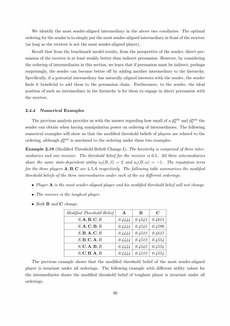
Example 2.19 (Modified Threshold Beliefs Change I). The hierarchy is comprised of three inter-

mediaries and one receiver. The threshold belief for the receiver is 0.5. All three intermediaries

share the same state-dependent utility uI(B, β) = 2 and uI(B,α) = −1. The reputation term

for the three players A,B,C are 4, 5, 6 respectively. The following table summarizes the modified

threshold beliefs of the three intermediaries under each of the six different orderings.

• Player A is the most sender-aligned player and his modified threshold belief will not change.

• The receiver is the toughest player.

• Both B and C change.

Modified Threshold Belief A B C

S,A,B,C, R 0.4444 0.4545 0.4615

S,A,C,B, R 0.4444 0.4545 0.4590

S,B,A,C, R 0.4444 0.4512 0.4615

S,B,C,A, R 0.4444 0.4512 0.4554

S,C,A,B, R 0.4444 0.4545 0.4554

S,C,B,A, R 0.4444 0.4512 0.4554

The previous example shows that the modified threshold belief of the most sender-aligned

player is invariant under all orderings. The following example with different utility values for

the intermediaries shows the modified threshold belief of toughest player is invariant under all

orderings.

30

Example 2.20 (Modified Threshold Beliefs Change II). The hierarchy is comprised of three inter-

mediaries and one receiver. The threshold belief for receiver is 0.5. All three intermediaries share

the same state-dependent utility uI(B, β) = 1 and uI(B,α) = −2. The reputation term for the

three players A,B,C are 4, 5, 6 respectively. The following table summarizes the modified threshold

beliefs of the three intermediaries under each of the six different orderings. We can observe that

• The receiver is the most sender-aligned player.

• A is the toughest player and his modified threshold belief will not change.

• Both B and C change.

Modified Threshold Belief A B C

S,A,B,C, R 0.5556 0.5455 0.5385

S,A,C,B, R 0.5556 0.5455 0.5410

S,B,A,C, R 0.5556 0.5488 0.5385

S,B,C,A, R 0.5556 0.5488 0.5446

S,C,A,B, R 0.5556 0.5455 0.5446

S,C,B,A, R 0.5556 0.5488 0.5446

3 Private Information

We now consider the scenario that each player in the chain of persuasion has private infor-

mation, represented in the model by their types. Different types of players (intermediaries and

receiver) may have different values of u(B,α), u(B, β), and different types of intermediaries may

also have different values of the reputation gain term. For simplicity the private information

represented by a single random variable, can be considered as being directly over each intermedi-

ary’s modified threshold belief and receiver’s threshold belief. Later in this section, we show this

simplification is reasonable.

We use ΘR to denote the type space for the receiver and Θj to denote the type space for

intermediary j. We assume that |ΘR| ≤ ∞ and |Θj | ≤ ∞ for all j. The cumulative distribu-

tion function of prior distribution of the receiver’s type is common knowledge and is denoted

as FR : ΘR → [0, 1]. The cumulative distribution function of prior distribution of intermediary

j’s type is common knowledge and is denoted as Fj : Θj → [0, 1]. These cumulative distribu-

tion functions are able to directly represent the modified threshold beliefs in place of the triple

(Rj , uj(B,α), uj(B, β)).

Each player’s payoff is affected by the belief of the previous intermediary as well as the type

realizations of subsequent players, but not the realization of the types of players preceding him in

the path of persuasion. Let θR be a representative element of ΘR and let θj be a representative

element of Θj . Compared to the benchmark model, the utilities can be represented by conditional

utility expressions

31

• The utility function of the receiver depends on private type θR, uR(d, t|θR). Then threshold

belief p̃R(θR) = −uR(B,α|θR)uR(B,β|θR)−uR(B,α|θR)

is a sufficient statistic to characterize the behavior of

receiver.

• The utility function of intermediary j depends on private type θj , uj(d, t|θj).

• Furthermore, the reputation term of intermediary j is now a random parameter depends on

private type θj , Rj(θj).

Therefore, our original assumptions are adjusted to accommodate the private information setting

as follows

Assumption 3.1. The minimum reputation gain has a lower bound, for all θj ∈ Θj

Rj(θj) > max(− uj(B,α|θj), uj(B, β|θj)

)(13)

Nonetheless, the randomness of Rj(θj) can be incorporated into p̃Ij(θj) because Rj(θj) is only

used to determine p̃Ij(θj) when analyzing behavior in the response stage of intermediary j. When

analyzing the behavior for the persuasion stage of intermediary j − 1, the random component is

already captured by the modified threshold beliefs {p̃Ij(θj)}θj∈Θj .

We denote a distribution of posteriors by τ ∈ ∆(∆(T )). Therefore, the optimal strategy for a

player is a function τ(p) : ∆(T ) −→ ∆(∆(T )). The optimal strategy is a function which generates

a distribution of posteriors based on one’s own belief about the state, ie. a function from a

posterior ∆(T ) to distribution of posteriors ∆(∆(T )). Keeping with previous terminology, in the

private information case, no disclosure refers to the situation that the message of the intermediary

in question is fully uninformative. When |T | = 2, the degree of freedom (number of parameters

of the system that may vary independently) of the posterior distribution is 1. Here for a binary

distribution, when probability of one type is given as p, then the probability of the other type

is 1 − p. In other words, we can use one parameter to denote the distribution. Therefore, the

distribution of posteriors by τ ∈ ∆([0, 1]) and τ(p) : [0, 1] −→ ∆([0, 1]). Hence the concavification

process works on a one dimensional function V (p). The following proposition shows that, for such

a one dimensional function, the result of concavification must take a special form, which guarantees

the computational tractability of further analysis on private information.

Proposition 3.2. In the case of private information, the optimal strategy is always equivalent to

a partition over [0, 1] by a series of cutoff values 0 = γ1 < · · · < γl = 1, each interval is associated

with a strategy taken from {C,D}, where C is full concealment, and D represents partial disclosure

that generates two posteriors. When prior p is located in the range [γk, γk+1] with an associated

strategy C, the optimal strategy is no disclosure. When prior p is located in the range [γk, γk+1]with

an associated strategy D, the optimal strategy induces two posteriors, γk, γk+1.

The proposition states that under private information, the result of optimal Bayesian persuasion

must take this special form. Cutoff values are determined by concavification, later we will provide

32

an algorithm to return all cutoff values. The full disclosure policy is equivalent to γ1 = 0, γ2 = 1

and D when p ∈ [0, 1]. The full concealment policy is equivalent to γ1 = 0, γ2 = 1 and C when

p ∈ [0, 1]. The optimal policy in the prosecution example in Kamenica and Gentzkow (2011) is

equivalent to the following, D p ∈ [0, 0.5]

C p ∈ [0.5, 1]

Assume that utility function V (·) is defined over probability space [0, 1]. The proof of the

proposition follows from several observations. Note that this proposition hold not only in hierar-

chical Bayesian persuasion case, but also in other situations as long as the state is binary.

We first establish the following Lemma, which illustrates that two posteriors are sufficient for

implementing optimal Bayesian persuasion signal.

Lemma 3.3. If C is not the optimal strategy for belief p, then all possible optimal disclosure

policies are outcome-equivalent to a policy that consists of two posteriors that are minimum and

maximum of the original posteriors profile.

Proof. If the posteriors profile consists of more than 2 posteriors, consider the arbitrary three

posteriors in profile, p1 < p2 < p3. We claim that

V (p2) =p2 − p1

p3 − p1V (p3) +

p3 − p2

p3 − p1V (p1) (14)

in other words, p2 and

p1 with probabilityp3 − p2

p3 − p1

p3 with probabilityp2 − p1

p3 − p1

are mutually replaceable. Otherwise, there exists a better disclosure policy, and the original one

cannot be optimal. If the weight of p2 in the posterior is q, then we increase the weight of p1 byp3−p2p3−p1 q and p3 by p2−p1

p3−p1 q, then we obtain another optimal policy that contains fewer posteriors.

This procedure can be repeated until there are only two posteriors included. Furthermore, these

two posteriors are the minimum and maximum of the original posteriors, respectively.

From now on, without loss of generality, we assume that if no disclosure is not optimal for

belief p, then optimal Bayesian persuasion must consist of two posteriors. The following lemma

builds the bridge from analysis of a specific prior to analysis of all priors in some interval.

Lemma 3.4. If it is optimal to induce posteriors pl < p < ph for belief p, then it is optimal to

induce posteriors pl < p′ < ph for all beliefs p′ ∈ (pl, ph).

33

Proof. The following disclosure policy is optimal for belief p,

ph with probabilityp− plph − pl

pl with probabilityph − pph − pl

Assume (for a contradiction) that there exists a p′ ∈ (pl, ph) such that inducing beliefs p′l < p′ < p′his better than inducing beliefs pl < p < ph, which indicates

p′ − p′lp′h − p′l

V (p′h) +p′h − p′

p′h − p′lV (p′l) >

p′ − plph − pl

V (ph) +ph − p′

ph − plV (pl) (15)

Then we can find a better disclosure policy for belief p,

ph with probabilityp− plph − pl

− ε p′ − plph − pl

pl with probabilityph − pph − pl

− εph − p′

ph − pl

p′h with probability εp′ − p′lp′h − p′l

p′l with probability εp′h − p′

p′h − p′l

where 0 < ε < min( p−plp′−pl ,ph−pph−p′ ). (Contradiction)

The previous lemma illustrates algebraically that if for some probability p ∈ [γ′, γ′′], it is

optimal to generate two posteriors γ′ and γ′′, then these two posteriors are optimal for all prior

probabilities between γ′ and γ′′. We can prove this lemma geometrically as following. From the

optimality for p to generate γ′ and γ′′, function V must lie below the line connecting (γ′, V (γ′))

and (γ′′, V (γ′′)) for all p ∈ [0, 1], which gives us an upper bound of concave closure V̂ . Meanwhile,

it is possible for all priors between γ′ and γ′′ to reach this upper bound, which proves its optimality.

The next lemma demonstrates how we can merge many intervals for the same prior if we have

already found several pairs of γ′, γ′′.

Lemma 3.5. If there exist multiple optimal disclosure policies for belief p, associated posteriors

are denoted as {pil, pih}i=1,··· ,n, then a disclosure policy generating posteriors as mini pil and maxi p

ih

is also optimal.

34

Proof. It is also optimal for the following policy,

p1h with probability

1

m

p− p1l

p1h − p1

l

p1l with probability

1

m

p1h − p

p1h − p1

l· · · · · · · · ·

· · · · · · · · ·

pih with probability1

m

p− pilpih − pil

pil with probability1

m

pih − ppih − pil

· · · · · · · · ·

· · · · · · · · ·

pmh with probability1

m

p− pmlpmh − pml

pml with probability1

m

pmh − ppmh − pml

By Lemma 3.3, this is outcome equivalent to generating mini pil and maxi p

ih.

Finally, we show that for all prior distributions for which no disclosure is not the optimal

strategy, we can always find the longest interval.

Lemma 3.6. If C is not optimal for belief p, there exists pl < p and ph > p such that it is optimal

to induce posteriors pl and ph. There exists no other optimal policy with p′l and p′h such that

0 ≤ p′l < pl or ph < p′h ≤ 1.

Proof. Since no disclosure is not optimal for belief p, by Lemma 1, we assume it is optimal to

induce pL and pH . Hence the linear function goes through (pL, V (pL)) and (pH , V (pH)) is no less

than the original function V everywhere in the interval [0, 1],

V (p) ≤ p− pLpH − pL

V (pH) +pH − ppH − pL

V (pL) (16)

If for some p, V (p) < p−pLpH−pLV (pH) + pH−p

pH−pLV (pL), then it cannot be included in the optimal

posteriors profile. In other words, only solution to the following equation can be introduced in

optimal posteriors profile,

V (p) =p− pLpH − pL

V (pH) +pH − ppH − pL

V (pL) (17)

Assume this equation has multiple solutions p1, · · · , pm ∈ [0, 1]. Let pl and ph be the minimum

and maximum. If pl = 0 or ph = 1, it is trivial we cannot find such p′l and p′h. If pl > 0, then

35

V (p′l) <p−pLpH−pLV (pH) + pH−p

pH−pLV (pL) for all p′l ∈ [0, pl) because pl is the minimum solution. If

ph < 1, then V (p′h) < p−pLpH−pLV (pH) + pH−p

pH−pLV (pL) for all p′h ∈ (ph, 1] because pl is the maximum

solution.

Proof of Proposition 3.2. Consider the following divide and conquer algorithm for p ∈ [L,H]. Any

posteriors that are not belonging to [L,H] cannot be introduced in optimal posteriors profile for

prior p ∈ [L,H]. We begin with an arbitrary prior p ∈ [L,H].

Case (1). If C is optimal, then we can find the largest connected interval [pl, ph] including p

that C is optimal by trials, and run the algorithm in sub-interval [L, pl] and [ph, H].

Case (2). If C is not optimal, we can always find pl and ph satisfying the condition of Lemma

4. It is optimal to induce pl and ph when p ∈ [pl, ph] and never optimal for p ∈ [L, pl) ∪ (ph, H] to

induce any posterior in [pl, ph].

Then, any posteriors that are not belongs to [L, pl) cannot be introduced in optimal posteriors

profile for prior in [L, pl]; any posteriors that are not belongs to [pH , H] cannot be introduced in

optimal posteriors profile for prior in (pH , H]. Then, we run the algorithm for both sub-interval,

[L, pl) and (pH , H]. The following pseudo-code illustrates the procedure,

Algorithm 1 Find Cutoff Values Inside [L,H]

1: For arbitrary p2: Find largest interval [pl, ph] that has same strategy with p.3: if pl = L and ph = H then4: return5: end if6: if pl > L then7: Report pl as cutoff values.8: Find Cutoff Values Inside [L, pl].9: end if

10: if ph < H then11: Report ph as cutoff values.12: Find Cutoff Values Inside [ph, H].13: end if

3.1 Persuading the Receiver

In the previous section, we showed that for all players in the hierarchical Bayesian persuasion

game, their optimal strategies take the specific form described in Proposition 3.2. Thus, we

can continue to solve the equilibrium by backward induction without solving for the closed form

expression of value function V as well as its concave closure V̂ for specific players. To examine the

persuasion of the receiver, we first consider a simple model without intermediaries as illustrated in

Kamenica and Gentzkow (2011). The state-dependent payoff of the receiver is random and may

36

take on several values. For each realization of payoffs, we can compute the threshold belief of

such realizations. Those cutoff beliefs are then sufficient for the sender. The sender takes a similar

strategy as in Kamenica and Gentzkow (2011), except that he needs to decide what posterior belief

he wants to generate, which is 0.5 in the Kamenica and Gentzkow (2011) prosecutor example. We

demonstrate that such a posterior belief must be one of the possible values of the threshold belief of

the receiver. Mathematically, all γ values (except the two endpoints 0,1) introduced in Proposition

3.2 must take the threshold belief for some type of receiver. However, not all values of threshold

belief are taken as γs. Example 3.7 below provides insights. Compared with benchmark model,

with private information, for some posteriors, some types of receivers may reject the proposal.

Formally, if a B-preferred sender induces belief p in the receiver, then the probability that the

receiver finally chooses B can be expressed as the probability that the receiver has lower threshold

belief than p,

VBR(p) = Pr(d = B|p) = EθR [I(p̃R(θR) ≥ p)|θR] = FR(p) (18)

where FR(p) denotes the cumulative distribution function of the threshold belief of the receiver.

VBR(p) has the following properties, (1) weakly increasing, (2) right-continuous, (3) piecewise

constant (if |ΘR| <∞).

For a better understanding, we use the following cumulative distribution function as a discrete

example to illustrate the construction of V̂BR and V̂AR as well as the optimal strategy represented

by Proposition 3.2.

Example 3.7. 17 Assume there are four different types of receivers,

1. 20 percent of the receivers have threshold belief 0.24;

2. 40 percent of the receivers have threshold belief 0.3;

3. 24 percent of the receivers have threshold belief 0.6;

4. 16 percent of the receivers have threshold belief 0.96.

We can derive the VBR(p) and VAR(p) for the receiver from the cumulative distribution function

,

VBR(p) = FR(p) =

0 p ∈ [0, 0.24)

0.2 p ∈ [0.24, 0.3)

0.6 p ∈ [0.3, 0.6)

0.84 p ∈ [0.6, 0.96)

1 p ∈ [0.96, 1]

VAR(p) = 1− FR(p) =

1 p ∈ [0, 0.24)

0.8 p ∈ [0.24, 0.3)

0.4 p ∈ [0.3, 0.6)

0.16 p ∈ [0.6, 0.96)

0 p ∈ [0.96, 1]

17In this example, the concave closure is a continuous function while the original function is right-continuous only.

37

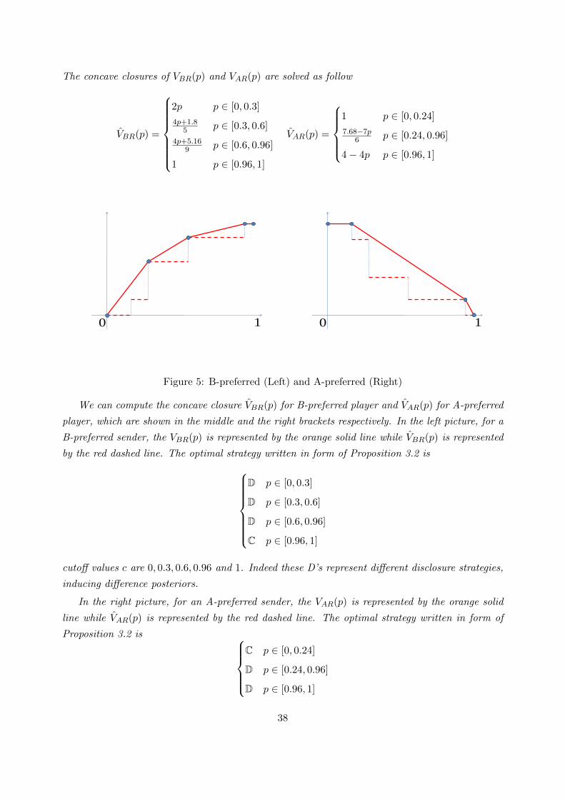
The concave closures of VBR(p) and VAR(p) are solved as follow

V̂BR(p) =

2p p ∈ [0, 0.3]

4p+1.85 p ∈ [0.3, 0.6]

4p+5.169 p ∈ [0.6, 0.96]

1 p ∈ [0.96, 1]

V̂AR(p) =

1 p ∈ [0, 0.24]

7.68−7p6 p ∈ [0.24, 0.96]

4− 4p p ∈ [0.96, 1]

10 10

Figure 5: B-preferred (Left) and A-preferred (Right)

We can compute the concave closure V̂BR(p) for B-preferred player and V̂AR(p) for A-preferred

player, which are shown in the middle and the right brackets respectively. In the left picture, for a

B-preferred sender, the VBR(p) is represented by the orange solid line while V̂BR(p) is represented

by the red dashed line. The optimal strategy written in form of Proposition 3.2 is

D p ∈ [0, 0.3]

D p ∈ [0.3, 0.6]

D p ∈ [0.6, 0.96]

C p ∈ [0.96, 1]

cutoff values c are 0, 0.3, 0.6, 0.96 and 1. Indeed these D’s represent different disclosure strategies,

inducing difference posteriors.

In the right picture, for an A-preferred sender, the VAR(p) is represented by the orange solid

line while V̂AR(p) is represented by the red dashed line. The optimal strategy written in form of

Proposition 3.2 is C p ∈ [0, 0.24]

D p ∈ [0.24, 0.96]

D p ∈ [0.96, 1]

38

cutoff values c are 0, 0.24, 0.96 and 1.

For the further analysis, we characterize some properties for V̂BR(p) and V̂AR(p),

1. Both V̂BR(p) and V̂AR(p) are concave

2. V̂BR(1) = V̂AR(0) = 1

3. V̂BR(0) = V̂AR(1) = 0

4. V̂BR is strictly increasing when V̂BR(p) < 1 while V̂AR is strictly decreasing when V̂BR(p) < 1.

Lemma 3.8. V̂BR(p) + V̂AR(p) > 1 for p ∈ (0, 1) unless FR(p) = p.

Proof. The concave closure V̂BR(p) (or V̂AR(p)) is the smallest concave function that is everywhere

weakly greater than FR(p) (or 1−FR(p)). Therefore, V̂BR(p) ≥ p for p ∈ (0, 1) while V̂AR(p) ≥ 1−pfor p ∈ (0, 1). Assume there exists a p′ ∈ (0, 1) such that FR(p′) 6= p′. If FR(p′) > p′, then

V̂BR(p) > p for all p ∈ (0, 1). Since V̂AR(p) ≥ 1 − p for p ∈ (0, 1), V̂BR(p) + V̂AR(p) > 1 for

p ∈ (0, 1). If FR(p′) < p′, then V̂AR(p) > 1 − p for all p ∈ (0, 1). Since V̂BR(p) ≥ p for p ∈ (0, 1),

V̂BR(p) + V̂AR(p) > 1 for p ∈ (0, 1).

This lemma will be useful in section 3.4.1 during discussion of the special case of the receiver with

uniformly distributed private information.

3.2 Persuading the Last Intermediary

Just as in the benchmark model, the strategy of an intermediary consists of two parts, the

response stage and the persuasion stage. For the last intermediary in the sequence, his or her

behavior in the persuasion stage is the same as that of a sender in the model without intermediaries,

which is analyzed in the previous subsection. Now, we examine the response stage. We must

characterize whether intermediary n responds to intermediary n−1 with A or B, when the induced

belief is p, given his type θn. The most important question is whether the modified threshold belief

defined in the benchmark model still exists. If so, is it the unique one?

We first define the expected utility for intermediary n with the following features

1. Responding A/B to intermediary n− 1

2. Intermediary n generates posterior p to the receiver

3. The type of the intermediary n is θn

4. The type of the receiver is θR

39

by the expressions

Un(p|A, θn, θR) = Pr(d = A)Rn + Pr(d = B)(pun(B, β|θn) + (1− p)un(B,α|θn)

)= (1− I(p|θR))Rn + I(p|θR)(pun(B, β|θn) + (1− p)un(B,α|θn))

Un(p|B, θn, θR) = Pr(d = A) · 0 + Pr(d = B)(Rn + pun(B, β|θn) + (1− p)un(B,α|θn)

)= I(p|θR)(Rn + pun(B, β|θn) + (1− p)un(B,α|θn))

respectively, where boolean variable I(p|θR) = I(p̃R(θR) ≤ p) ∈ {0, 1} represents whether receiver

will choose action B or not when the intermediary passes posterior p to receiver. Firstly, it is

easy to see that Un(p|B, θn, θR) is increasing in p because when p increases, both I(p|θR) and

Rn + pun(B, β) + (1− p)un(B,α) are nonnegative and increasing. Secondly, we have the following

boundary values, which help us prove the existence and uniqueness of the modified threshold belief.

Un(0|A, θn, θR) = Rn

Un(1|A, θn, θR) = un(B, β)

Un(0|B, θn, θR) = 0

Un(1|B, θn, θR) = Rn + un(B, β)

In addition, we have Un(p|A, θn, θR) ≤ Rn − I(p|θR)(Rn − un(B, β)) ≤ Rn for all p. Therefore,

if we take the expectation over θR, we have the expected utility for A-preferred and B-preferred

intermediaries n given his type is θn under two extreme posteriors (0 and 1),

EθR [Un(0|A, θn, θR)] = Rn

EθR [Un(1|A, θn, θR)] = un(B, β)

EθR [Un(0|B, θn, θR)] = 0

EθR [Un(1|B, θn, θR)] = Rn + un(B, β)

Then by Bayesian persuasion, for an A-preferred player, the best he can achieve is the concave

closure of EθR [Un(p|A, θn, θR)], Co(EθR [Un(p|A, θn, θR)]); for a B-preferred player, the best he can

achieve is the concave closure of EθR [Un(p|B, θn, θR)], Co(EθR [Un(p|B, θn, θR)]). We then need to

compare whether response A or B is better.

We claim that Co(EθR [Un(p|A, θn, θR)]) is decreasing in p while Co(EθR [Un(p|B, θn, θR)]) is

increasing in p. The latter statement holds because each Un(p|B, θn, θR) is increasing. As for

the former statement, we have shown that Un(p|A, θn, θR) ≤ Rn and hence EθR [Un(p|A, θn, θR)] ≤Rn. Since Co(EθR [Un(p|A, θn, θR)]) is a concave function, if the derivative is positive for some

value p, then Co(EθR [Un(p|A, θn, θR)]) is strictly increasing for all probabilities [0, p]. However,

40

Co(EθR [Un(p|A, θn, θR)]) cannot exceed Rn = Co(EθR [Un(0|A, θn, θR)]). This provides a contra-

diction.

The following lemma illustrates the single crossing property.

Lemma 3.9. Co(EθR [Un(p|A, θn, θR)]) = Co(EθR [Un(p|B, θn, θR)]) has a unique solution and we

define it as p = p̃In(θn).

Proof. Given that Co(EθR [Un(p|B, θn, θR)]) is concave increasing, Co(EθR [Un(p|B, θn, θR)]) is strictly

increasing when Co(EθR [Un(p|B, θn, θR)]) ∈ [0, Rn+un(B, β)). Therefore, Co(EθR [Un(p|B, θn, θR)])

is strictly increasing when its value is inside the interval [un(B, β), Rn]. Since Co(EθR [Un(p|A, θn, θR)])

is concave decreasing, the solution exists uniquely.

Hence, there exists a threshold value p̃In(θn) for type θn, called the modified threshold belief

such that intermediary n is indifferent between choosing A and B in response stage. Here, we can

see that the modified threshold belief p̃In(θn) is sufficient to represent the behavior of intermedi-

ary n with type θn, which justifies our definition about the cumulative distribution in Section 3

(paragraph 2).

Now we move to the persuasion stage of intermediary n−1. Take the B-preferred intermediary

n − 1 as an example, we first compute the probability that the receiver chooses B given that

intermediary n has type θn when intermediary n−1 passes posterior p to intermediary n. If p does

not exceed p̃In(θn), then intermediary n with type θn becomes A-preferred and tries to persuade

receiver to maximize the probability of choosing A (which is V̂AR(p)), hence the probability of

choosing B is 1 − V̂AR(p). If p exceeds p̃In(θn), then intermediary n with type θn becomes B-

preferred and tries to persuade the receiver to maximize the probability of choosing B (which is

V̂BR(p)). Therefore, the probability that the receiver chooses B is defined as

VBn(p|θn) =

1− V̂AR(p) p < p̃In(θn)

V̂BR(p) p ≥ p̃In(θn)(19)

where both V̂AR(p) and V̂BR(p) are derived from the previous subsection and are irrelevant to θn.

Therefore, on behalf of intermediary n − 1, when he passes p to intermediary n, the probability

that B is chosen is the expectation of VBn(p|θn) taken over θn.

VBn(p) =

∫θn

VBn(p|θn)dFn(θn) (20)

Likewise, if intermediary n− 1 is A-preferred, VAn(p) has the following expression

VAn(p) =

∫θn

VAn(p|θn)dFn(θn) (21)

41

where

VAn(p|θn) =

V̂AR(p) p ≤ p̃In(θn)

1− V̂BR(p) p > p̃In(θn)(22)

Hence, we can calculate V̂Bn(p) = Co(VBn(p)) and V̂An(p) = Co(VAn(p)). Proposition 3.2 tells us

that these calculation processes are straightforward. Hence, we can use V̂An and V̂Bn directly.

Although the calculation process of concave closure is generally difficult, Proposition 3.2 told

us, with a binary state, the optimal strategy of intermediary n − 1 is always equivalent to a

partition associated with strategy C,D and can be computed in polynomial time efficiently, even

with infinity number of type. Then, we can recover the strategies from V̂An and V̂Bn.

3.3 Persuading the Intermediary j

We now analyze how to persuade intermediary j for a general j. Mathematically, this means

solving V̂Bj and V̂Aj from V̂B,j+1 and V̂A,j+1 (In section 3.2, we solve V̂Bn and V̂An from V̂BR and

V̂AR). The methodology for proving the single crossing property is exactly the same as previously.

For any intermediary j, the optimal disclosure strategy in the persuasion stage is unrelated to

his own type. However, the modified threshold belief of intermediary j depends on his own type.

Please refer to the Appendix for details.

3.4 Some Special Cases

While the previous subsection derived results for the general case, it is helpful to examine some

special cases in order to gain specific insights which cannot be easily observed from the general

results. We first discuss the special case that the receiver has a uniformly distributed type. We

then separately consider the special case that only the receiver has private information.

3.4.1 Uniformly Distributed Receiver

The previous analysis have focused on understanding when the sender benefits from persua-

sion and deriving the optimal signal. However, when is persuasion ineffective? The case of a

uniformly type-distributed receiver provides insights on this question. The following proposition

shows that for a uniformly type-distributed receiver, Bayesian persuasion cannot do any better

than degenerate strategies, including full concealment and full disclosure.

Proposition 3.10. Bayesian persuasion cannot generate higher revenue for all p ∈ [0, 1] if

FR(p) = p.

Proof. When FR(p) = p, we have VBR(p) = V̂BR(p) = p and VAR(p) = V̂AR(p) = 1 − p. By

induction, we can prove that VBj = V̂Bj = p and VAj(p) = V̂Aj(p) = 1− p for all j.

42

This proposition applies Lemma 3.8. This is not the only situation that persuasion is ineffec-

tive. As long as VBj(p) = p and VAj(p) = 1 − p for some intermediary j, then for all preceding

intermediaries, persuasion is ineffective.

3.4.2 Deterministic Intermediaries

Another special case is that only the receiver has private information while all intermediaries’

information are public. This case is somewhere between benchmark model and general version of

private information model. Hence, when we derive VBn(p) and VAn(p), there will be no uncertainty

and the results will be

VBn(p) =

1− V̂AR(p) p < p̃In

V̂BR(p) p ≥ p̃In

VAn(p) =

V̂AR(p) p ≤ p̃In

1− V̂BR(p) p > p̃In

and the concave closures are

V̂Bn(p) =

pV̂BR(p̃In)

p̃Inp < p̃In

V̂BR(p) p ≥ p̃In

V̂An(p) =

V̂AR(p) p ≤ p̃In(1−p)V̂AR(p̃Ij)

1−p̃In p > p̃In

Applying the same induction process as Theorem 2.5, we can derive the general formula for

V̂B,j+1(p) and V̂A,j+1(p).

Theorem 3.11. For B-preferred intermediary j with incoming belief p, the probability of B in

optimal persuasion is V̂B,j+1(p), and for A-preferred intermediary j with incoming belief p, the

probability of A in optimal persuasion is V̂A,j+1(p), where

V̂B,j+1(p) =

pV̂BR(p̃max

j )

p̃maxj

p < p̃maxj

V̂BR(p) p ≥ p̃maxj

V̂A,j+1(p) =

V̂AR(p) p ≤ p̃minj

(1−p)V̂AR(p̃minj )

1−p̃minj

p > p̃minj

where V̂BR = Co(FR) and V̂AR = Co(1−FR). p̃maxj and p̃min

j are defined as p̃maxj = max

({p̃Ik}nk=j+1, 0

)and p̃min

j = min({p̃Ik}nk=j+1, 1

).

p̃maxj and p̃min

j do not include p̃R anymore, since the information of p̃R is already captured by

43

V̂AR(p) and V̂BR(p). When j = n, p̃maxj = 0 and p̃min

j = 1.

The equilibrium strategy is same as the benchmark model. Both the one-step equilibrium and

myopic equilibrium, as well as other equilibria situated between these two extreme cases remain

as equilibria. However, the differences are (1) when p > p̃maxj , for B-preferred intermediary j, the

probability of decision B is no longer 1; (2) when p < p̃minj , for A-preferred intermediary j, the

probability of decision A is no longer 1.

4 Endogenous Reputation

The exogenous reputation term in the model up to now can be seen as the discounted future

benefit in current terms. However, the nature of this benefit may be based on the relationship

implied by successful recommendation. For example, assume that a professor writes a recommen-

dation letter for a student to the admission committee and the student is accepted to the program.

Firstly, this long-run relationship may generate benefits for the professor compared to a situation

where the student is rejected from the program. Secondly, when the rejection is observed by other

students, fewer students may approach the professor in the future. Effect from the other side may

also exist. For example, when the professor recommended negatively while the student still got in,

fewer students may approach this professor in the future. These effects make the long-run benefit

potentially more important for the professor than the admission decision itself. However, up to

this point we have set the reputation gain from effective persuasion exogenous given.

In this section, we endogenize future benefits through an infinitely repeated game instead of

using the previously considered exogenous reputation term. In an infinitely repeated game setting,

the discounted future benefit is influenced by subsequent strategies, while the discounted future

benefit is used to find the equilibrium strategy as in previous section. The relationship between

the persuasion policy and the associated revenue function is shown in Figure 3.

The benchmark case merely considers the impact of future revenue on the optimal policy but

not the impact of the optimal policy on future revenue. Therefore, we apply dynamic programming

techniques to handle this endogenous influence. We show that the equilibrium essentially follows

the same pattern as before. We first consider the simpler case of one intermediary in the hierarchy,

then analyze the case of multiple intermediaries.

4.1 One Intermediary

Consider a repeated game with an infinite horizon. In the first stage, sender, receiver and

intermediary play a hierarchical Bayesian persuasion game drawn from the stage game set X. If

receiver took the same action that intermediary responded to the sender in time k, then another

hierarchical Bayesian persuasion game is played in time k+1, drawn from same stage game set X.

The sender and receiver may not be the same individuals as in previous stages. If the receiver took

the other action, intermediary is not considered credible anymore and receives η in all following

44

StationaryPolicy, u

Revenue Function, J

Compute revenue

Solve policy

u is taken in all upcoming stage

J will be attained in next stage

Figure 6: Iteration Process with One Intermediary

stages. In order to make it Markovian and hence solvable under dynamic programming, we assume

that the stage game in k + 1 only depends on the stage game in k, but we do not impose a

requirement for independence of the stage games. The probability that stage game in k + 1 is xb

given that the stage game in k is xa is defined as πab, which is irrelevant to k. Then the path of

stage games is a discrete time Markov chain.

Hence, in each stage, the state of the intermediary can be characterized by X ∪ {N} where

x ∈ X represents the stage game that an intermediary faces if involved, while N represents non-

involvement due to a previously failed recommendation. We assume that once a recommendation

fails, that intermediary will not be invited to participate in further persuasion processes anymore,

Pr(xk+1 = N |xk = N) = 1 (23)

Note that this assumption is for simplicity only, and that the results hold for any situation

where the probability of being able to participate in future persuasion stage games is less than 1,

conditional on a failed recommendation.

The model is thus a dynamic control problem (or a Markovian decision problem) with station-

ary18 discrete system xk+1 = f(xk, uk, wk), where xk represents the state variable, uk represents

the Bayesian persuasion strategy and wk represents a disturbance that depends on xk, uk only. In

this section, we apply lots of notation from control theory and dynamic programming. No partic-

ipation, N, is an absorbing state. The Bayesian persuasion strategy consists of two parts, one in

each stage (response and persuasion stages). The disturbance wk exists because the outcome of

Bayesian persuasion is probabilistic.

18homogeneity, time invariant

45

The utility g(x, u, w), for the intermediary in stage game x with policy u and randomness w,

is discounted by factor δ ∈ (0, 1) and bounded by M , ∀x, u, w, |g(x, u, w)| ≤M .19 We use Ju(x) to

represent the utility function given that the state is now x under policy u. We use J∗(x) to represent

the optimal utility function. Hence, J∗(N) = η1−δ . In the following assumption, δExJ∗(x|x 6= N)

represents the future discounted utility under the optimal policy. We use uI(d, t|x) to represent

the stage utility of the intermediary derived from decision d in state t.

Assumption 4.1. For all x ∈ X, max(− uI(B,α|x), uI(B, β|x)

)< δExJ∗(x|x 6= N)− ηδ

1−δ

δExJ∗(x|x 6= N)− ηδ1−δ is the incremental revenue from successful recommendation. Under this

assumption, the intermediary maximizes the probability of his preferred action in the persuasion

stage. Now, we move to the general policy. For revenue function J , we define mapping T as

(TJ)(x) = maxu

Ew{g(x, u, w) + δJ(f(x, u, w))} (24)

which denotes the optimal revenue function for the one-stage problem that has stage revenue g

and terminal cost δJ .

Lemma 4.2 (Convergence Theorem and Bellman Equation Theorem). The optimal revenue func-

tion satisfies

J∗(x) = limN→∞

(TNJ)(x) (25)

and

J∗(x) = (TJ∗)(x) (26)

Furthermore, J∗ is the unique solution of this equation.

Proof. The above two theorems can be proved by a contraction mapping fixed-point theorem [29].20

Although the optimal revenue is pinned down uniquely, the optimal policy is not necessarily

unique. We illustrate the optimal control policy u∗ under optimal revenue J∗. That is,

J∗(x) = E{g(x, u∗, w) + δJ∗(f(x, u∗, w))

}(27)

We claim that the optimal policy is a threshold policy with a unique threshold. Given stationary

policy u is employed by intermediary after time k, it is required that u maximizes the expected

utility given that u is applied in all subsequent stages.

u ∈ arg maxv

(g(x, v, w) + δJu(f(x, v, w))

)(28)

19This notation is applied in control theory and followed from Dynamic Programming and Optimal Control, VolumeII (Dimitri P. Bertsekas, 2012), http://athenasc.com/dpbook.html.

20For details, please refer to Dynamic Programming and Optimal Control, Volume II (Dimitri P. Bertsekas, 2012),http://athenasc.com/dpbook.html

46

The negative proposition tells us that if u is not a maximizer of g(x, u, w) + δJu(f(x, u, w)), u

cannot be an optimal policy. Given any non-threshold policy u, we can compute the expectation

of future benefits δJu(x)− ηδ1−δ and plug it into the reputation term. Then in time k, the optimal

policy should be a threshold policy via the same reasoning as the benchmark model. Hence, we

conclude the following lemma.

Lemma 4.3. The optimal policy in response stage is a threshold policy. Mathematically, in equi-

librium, there exists a threshold value p̃ depending on state x only such that (1) responses B when

incoming belief is larger than p̃; (2) responses A when incoming belief is smaller than p̃.

Last but not least, we prove the uniqueness of the modified threshold belief for the intermediary.

The policy u can be represented by a series of parameters p̃I(u|x), which is known as the modified

threshold belief under game x. Given J∗ and the stage game x, the reputation term can be

determined uniquely as in the benchmark case, and hence we can solve the optimal modified

threshold belief. We can also prove uniqueness by regarding J(x) as a continuous function of

{p̃I(u|x)}x∈X and using the continuity property. J(x) as well as the optimal threshold belief are

uniquely determined, but without a closed form solution in general, since both the game set and

policy set are infinite. However, with finite size of X, the value of J∗ can be solved iteratively by

numerical linear algebra.

Example 4.4 (Endogenized Reputation with |X| = 1).

Setup. There is only one possible stage game x. In this stage game, the prior probability is

p0 = Pr(β) = 0.2. The discount factor is δ = 0.9. η = −10 and hence J∗(N) = −100. The

receiver has threshold belief p̃R = 0.5, state-dependent utilities for the intermediary are given by

uI(B,α) = −1, uI(B, β) = 10.

Analysis. Assume that intermediary has threshold p̃I in the stage game. We need to calculate

the present value J(p̃I) if applying this threshold policy in all subsequent games. The sender

will generate two possible posteriors, max(p̃I , p̃R) with probability p0max(p̃I ,p̃R) and 0 with probability

1− p0max(p̃I ,p̃R) . The revenue in the stage game is hence

Eg(p̃I) =

p0p̃R

(p̃RuI(B, β) + (1− p̃R)uI(B,α)) p̃I < p̃R

p0p̃I

(p̃IuI(B, β) + (1− p̃I)uI(B,α)) p̃I > p̃R

=

1.8 p̃I < 0.5

2.2− 0.2p̃I

p̃I > 0.5

The present value of future benefit is hence J(p̃I) = Eg(p̃I)1−δ and δJ(p̃I) = δEg(p̃I)

1−δ for the time

horizon starting from the next period. Given this revenue function, we iteratively solve for the

optimal threshold policy. The payoff of the intermediary with response A and B are calculated

47

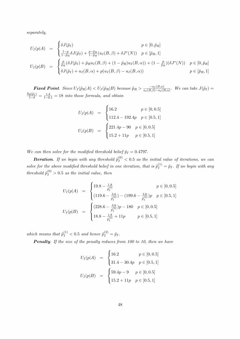
separately,

UI(p|A) =

δJ(p̃I) p ∈ [0, p̃R]

1−p1−p̃R δJ(p̃I) + p−p̃R

1−p̃R (uI(B, β) + δJ∗(N)) p ∈ [p̃R, 1]

UI(p|B) =

pp̃R

(δJ(p̃I) + p̃RuI(B, β) + (1− p̃R)uI(B,α)) + (1− pp̃R

)(δJ∗(N)) p ∈ [0, p̃R]

δJ(p̃I) + uI(B,α) + p(uI(B, β)− uI(B,α)) p ∈ [p̃R, 1]

Fixed Point. Since UI(p̃R|A) < UI(p̃R|B) because p̃R >−uI(B,α)

uI(B,β)−uI(B,α) . We can take J(p̃I) =Eg(p̃I)

1−δ = 1.81−0.1 = 18 into those formula, and obtain

UI(p|A) =

16.2 p ∈ [0, 0.5]

112.4− 192.4p p ∈ [0.5, 1]

UI(p|B) =

221.4p− 90 p ∈ [0, 0.5]

15.2 + 11p p ∈ [0.5, 1]

We can then solve for the modified threshold belief p̃I = 0.4797.

Iteration. If we begin with any threshold p̃(0)I < 0.5 as the initial value of iterations, we can

solve for the above modified threshold belief in one iteration, that is p̃(1)I = p̃I . If we begin with any

threshold p̃(0)I > 0.5 as the initial value, then

UI(p|A) =

19.8− 1.8

p̃(0)I

p ∈ [0, 0.5]

(119.6− 3.6

p̃(0)I

)− (199.6− 3.6

p̃(0)I

)p p ∈ [0.5, 1]

UI(p|B) =

(228.6− 3.6

p̃(0)I

)p− 180 p ∈ [0, 0.5]

18.8− 1.8

p̃(0)I

+ 11p p ∈ [0.5, 1]

which means that p̃(1)I < 0.5 and hence p̃

(2)I = p̃I .

Penalty. If the size of the penalty reduces from 100 to 10, then we have

UI(p|A) =

16.2 p ∈ [0, 0.5]

31.4− 30.4p p ∈ [0.5, 1]

UI(p|B) =

59.4p− 9 p ∈ [0, 0.5]

15.2 + 11p p ∈ [0.5, 1]

48

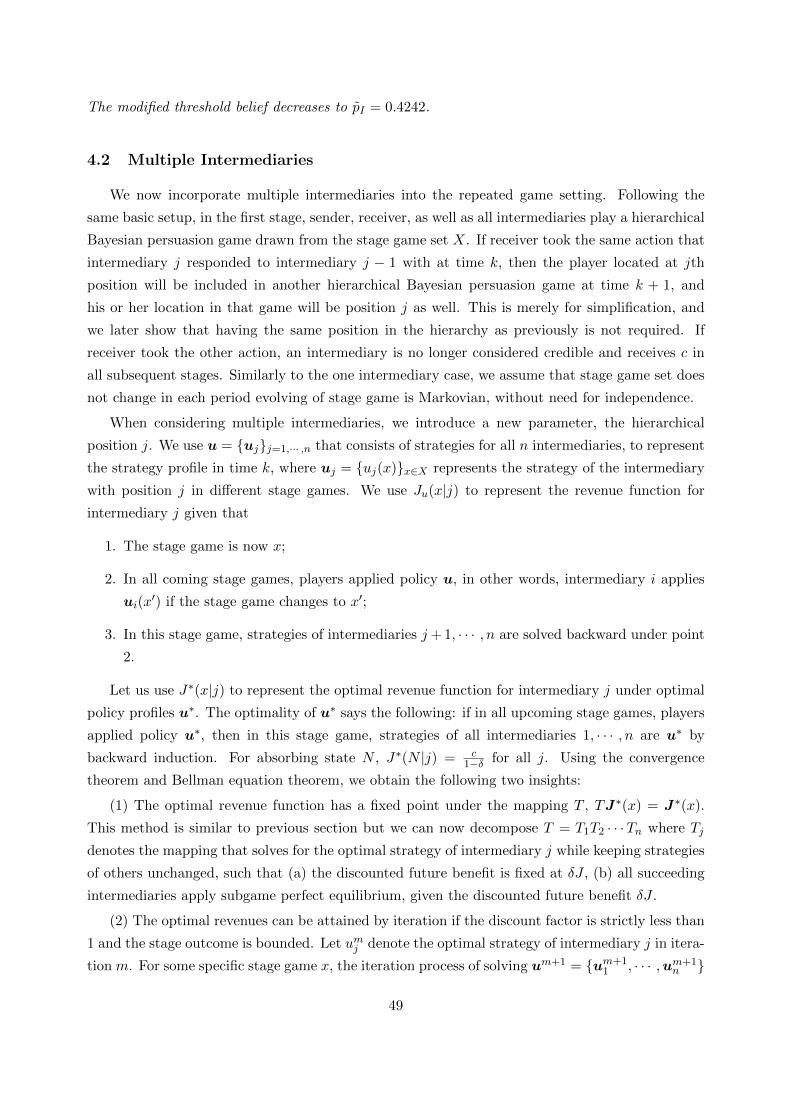
The modified threshold belief decreases to p̃I = 0.4242.

4.2 Multiple Intermediaries

We now incorporate multiple intermediaries into the repeated game setting. Following the

same basic setup, in the first stage, sender, receiver, as well as all intermediaries play a hierarchical

Bayesian persuasion game drawn from the stage game set X. If receiver took the same action that

intermediary j responded to intermediary j − 1 with at time k, then the player located at jth

position will be included in another hierarchical Bayesian persuasion game at time k + 1, and

his or her location in that game will be position j as well. This is merely for simplification, and

we later show that having the same position in the hierarchy as previously is not required. If

receiver took the other action, an intermediary is no longer considered credible and receives c in

all subsequent stages. Similarly to the one intermediary case, we assume that stage game set does

not change in each period evolving of stage game is Markovian, without need for independence.

When considering multiple intermediaries, we introduce a new parameter, the hierarchical

position j. We use u = {uj}j=1,··· ,n that consists of strategies for all n intermediaries, to represent

the strategy profile in time k, where uj = {uj(x)}x∈X represents the strategy of the intermediary

with position j in different stage games. We use Ju(x|j) to represent the revenue function for

intermediary j given that

1. The stage game is now x;

2. In all coming stage games, players applied policy u, in other words, intermediary i applies

ui(x′) if the stage game changes to x′;

3. In this stage game, strategies of intermediaries j+ 1, · · · , n are solved backward under point

2.

Let us use J∗(x|j) to represent the optimal revenue function for intermediary j under optimal

policy profiles u∗. The optimality of u∗ says the following: if in all upcoming stage games, players

applied policy u∗, then in this stage game, strategies of all intermediaries 1, · · · , n are u∗ by

backward induction. For absorbing state N , J∗(N |j) = c1−δ for all j. Using the convergence

theorem and Bellman equation theorem, we obtain the following two insights:

(1) The optimal revenue function has a fixed point under the mapping T , TJ∗(x) = J∗(x).

This method is similar to previous section but we can now decompose T = T1T2 · · ·Tn where Tj

denotes the mapping that solves for the optimal strategy of intermediary j while keeping strategies

of others unchanged, such that (a) the discounted future benefit is fixed at δJ , (b) all succeeding

intermediaries apply subgame perfect equilibrium, given the discounted future benefit δJ .

(2) The optimal revenues can be attained by iteration if the discount factor is strictly less than

1 and the stage outcome is bounded. Let umj denote the optimal strategy of intermediary j in itera-

tion m. For some specific stage game x, the iteration process of solving um+1 = {um+11 , · · · ,um+1

n }

49

are described as follows:

Tn : um+1n (x) ∈ arg max

unEw{g(x,u(n,m), w|n) + δJum(f(x,u(n,m), w)|n)}

Tn−1 : um+1n−1 (x) ∈ arg max

un−1

Ew{g(x,u(n− 1,m), w|n− 1) + δJum(f(x,u(n− 1,m), w)|n− 1)}

· · ·

T2 : um+12 (x) ∈ arg max

u2Ew{g(x,u(2,m), w|2) + δJum(f(x,u(2,m), w)|2)}

T1 : um+11 (x) ∈ arg max

u1Ew{g(x,u(1,m), w|1) + δJum(f(x,u(1,m), w)|1)}

where u(j,m) denotes the strategy that intermediaries with a label larger than j take in iteration

m + 1 while intermediaries with a label less than or equal to j take the following strategy in

iteration m,

u(n,m) = (um1 ,um2 , · · · ,umn−1,u

mn )

u(n− 1,m) = (um1 ,um2 , · · · ,umn−1,u

m+1n )

· · ·

u(2,m) = (um1 ,um2 , · · · ,um+1

n−1 ,um+1n )

u(1,m) = (um1 ,um+12 , · · · ,um+1

n−1 ,um+1n )

and

umj = {umj (x)}x∈X

Let us further examine the subscript u(n,m) at the term δJ that represents discounted future

revenue. When computing the iteration m+ 1, we use the optimal revenue computed at iteration

m for all n backward induction process in T1 to Tn. However, at iteration m + 1, each time we

solve for the new strategy of intermediary j, we assume that all subsequent players apply the new

strategy in current stage game in the spirit of backward induction. We show the iteration process

graphically in Figure 4.

In the one intermediary model, we showed that under some sufficient conditions, the optimal

strategy in the persuasion stage maximizes the likelihood of the preferred action. Additionally, the

optimal policy in the response stage is a threshold policy. When incorporating multiple interme-

diaries, we need to modify the assumptions to make it optimal to maximize the preferred action

in the persuasion stage. Previously, we showed the multi-intermediary version of the convergence

theorem and Bellman equation theorem. Therefore, with multiple intermediaries, the equilibrium

strategies follow the same pattern as the benchmark case and the case of endogenous reputation

with one intermediary.

When same position condition is violated, the agent in the jth position who recommends suc-

cessfully joins the next game and changes to a random position, we use δEjJu(n,m)(f(x,u(·,m), w)|j)to replace δJu(n,m)(f(x,u(·,m), w)|j). The previously mentioned results hold. Consider the ex-

50

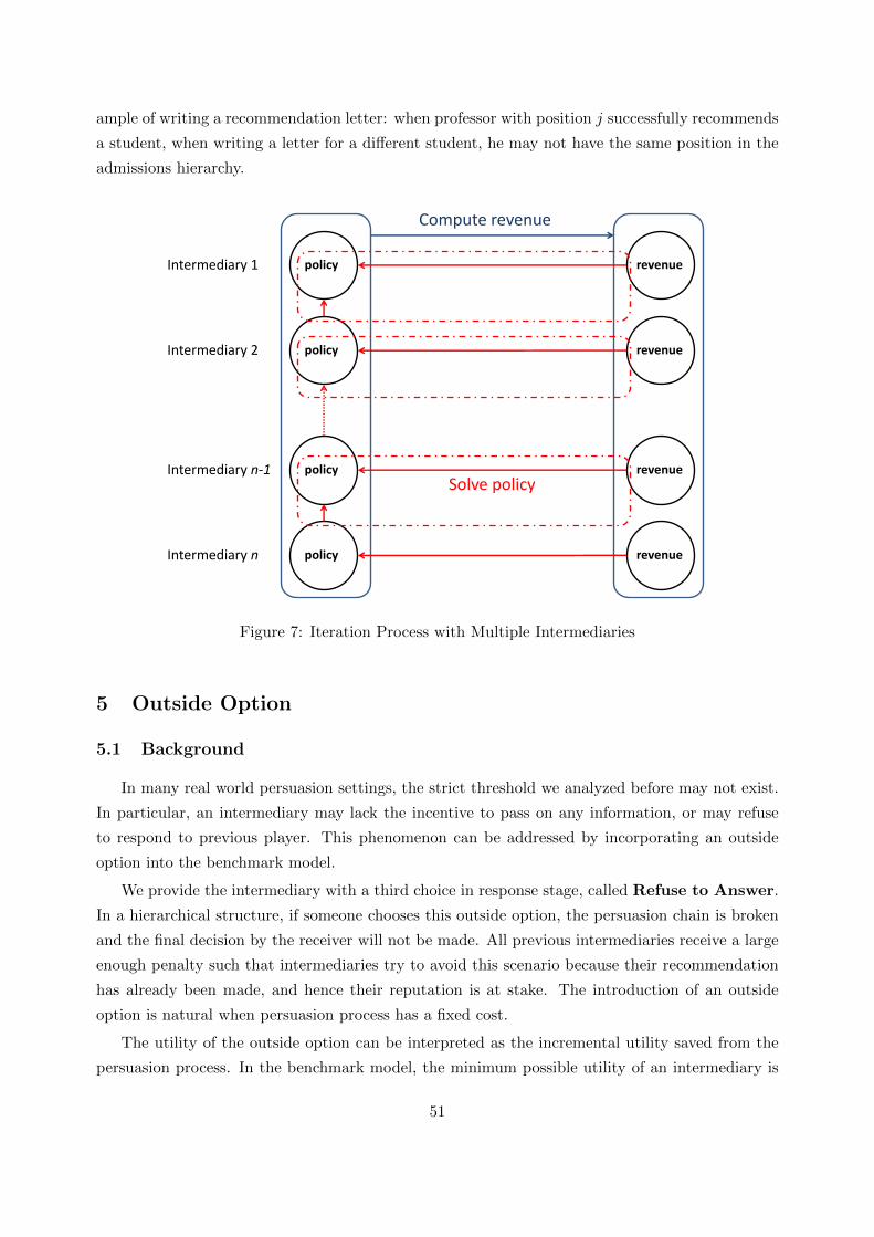
ample of writing a recommendation letter: when professor with position j successfully recommends

a student, when writing a letter for a different student, he may not have the same position in the

admissions hierarchy.

policy revenue Intermediary 1

policy revenue Intermediary 2

policy revenue Intermediary n-1

policy revenue Intermediary n

Compute revenue

Solve policy

Figure 7: Iteration Process with Multiple Intermediaries

5 Outside Option

5.1 Background

In many real world persuasion settings, the strict threshold we analyzed before may not exist.

In particular, an intermediary may lack the incentive to pass on any information, or may refuse

to respond to previous player. This phenomenon can be addressed by incorporating an outside

option into the benchmark model.

We provide the intermediary with a third choice in response stage, called Refuse to Answer.

In a hierarchical structure, if someone chooses this outside option, the persuasion chain is broken

and the final decision by the receiver will not be made. All previous intermediaries receive a large

enough penalty such that intermediaries try to avoid this scenario because their recommendation

has already been made, and hence their reputation is at stake. The introduction of an outside

option is natural when persuasion process has a fixed cost.

The utility of the outside option can be interpreted as the incremental utility saved from the

persuasion process. In the benchmark model, the minimum possible utility of an intermediary is

51

attained at the modified threshold belief. If the fixed cost Cj does not exceed such a minimum, the

equilibrium will not change. Otherwise, it is the case that intermediary j (1) Refuses to Answer

when the incoming belief falls into some interval [p̃Aj , p̃Bj ]; (2) responds A when the incoming belief

falls into some interval [0, p̃Aj ]; and (3) responds B when the incoming belief falls into some interval

[p̃Bj , 1]. It is possible that the expected gain from the outside option is so high such that some

intermediary always chooses Refuse to Answer. This double threshold policy reflects many

situations in reality where an individual has a belief in between ’yes’ and ’no’, and chooses to

remain silent.

Based on the benchmark model of Section 2, we set up a model incorporating the outside option

of intermediaries. The hierarchical structure includes one sender, one receiver and n intermediaries

just as before. The state space and action space are both binary. Besides receiving state-dependent

utility and reputation gains, each intermediary has a third option at the response stage, Refuse to

Answer, which provides utility Cj with certainty. For simplicity, if the outside option is exercised,

all preceding players receive a large enough punishment that can for simplicity be regarded as −∞.

5.2 Outside Option in Hierarchical Structure

Following backward induction, we first analyze the behavior of the last intermediary in the

chain. Under Assumption 2.1, the persuasion stage of the last intermediary is the same as previ-

ously, maximizing the preferred action. In the response stage, with different levels of C, interme-

diary n may have different levels of p̃An , p̃Bn . This is illustrated in the three figures below.

0 1

C

A

np B

npInp 0 1

C

A

np B

npInp 0 1

C

A

np B

npInp

Figure 8: Different Values of p̃An , p̃Bn with Different Levels of the Outside Option

• The figure on the left shows the case when C is comparable, 0 ≤ p̃An < p̃Bn ≤ 1.

• The figure in the middle shows the case when C is small, 0 < p̃An = p̃Bn < 1.

• The figure on the right shows the case when C is large, in which Refuse to Answer is the

dominant strategy.

To avoid the trivial case that some intermediary always chooses Refuse to Answer, we further

assume that the utility of outside option Cj for intermediary j will not exceed his reputation gain

Rj .

52

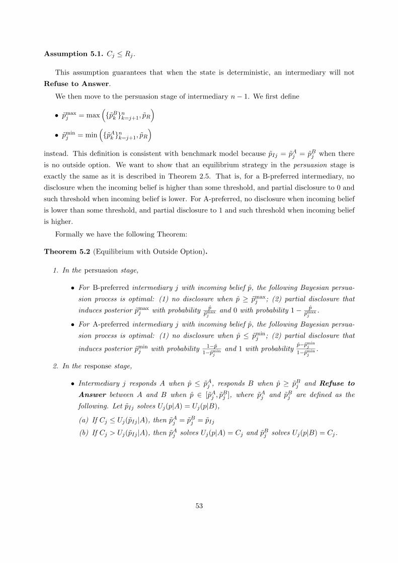
Assumption 5.1. Cj ≤ Rj.

This assumption guarantees that when the state is deterministic, an intermediary will not

Refuse to Answer.

We then move to the persuasion stage of intermediary n− 1. We first define

• p̃maxj = max

({p̃Bk }nk=j+1, p̃R

)• p̃min

j = min({p̃Ak }nk=j+1, p̃R

)instead. This definition is consistent with benchmark model because p̃Ij = p̃Aj = p̃Bj when there

is no outside option. We want to show that an equilibrium strategy in the persuasion stage is

exactly the same as it is described in Theorem 2.5. That is, for a B-preferred intermediary, no

disclosure when the incoming belief is higher than some threshold, and partial disclosure to 0 and

such threshold when incoming belief is lower. For A-preferred, no disclosure when incoming belief

is lower than some threshold, and partial disclosure to 1 and such threshold when incoming belief

is higher.

Formally we have the following Theorem:

Theorem 5.2 (Equilibrium with Outside Option).

1. In the persuasion stage,

• For B-preferred intermediary j with incoming belief p̂, the following Bayesian persua-

sion process is optimal: (1) no disclosure when p̂ ≥ p̃maxj ; (2) partial disclosure that

induces posterior p̃maxj with probability p̂

p̃maxj

and 0 with probability 1− p̂p̃maxj

.

• For A-preferred intermediary j with incoming belief p̂, the following Bayesian persua-

sion process is optimal: (1) no disclosure when p̂ ≤ p̃minj ; (2) partial disclosure that

induces posterior p̃minj with probability 1−p̂

1−p̃minj

and 1 with probabilityp̂−p̃min

j

1−p̃minj

.

2. In the response stage,

• Intermediary j responds A when p̂ ≤ p̃Aj , responds B when p̂ ≥ p̃Bj and Refuse to

Answer between A and B when p̂ ∈ [p̃Aj , p̃Bj ], where p̃Aj and p̃Bj are defined as the

following. Let p̃Ij solves Uj(p|A) = Uj(p|B),

(a) If Cj ≤ Uj(p̃Ij |A), then p̃Aj = p̃Bj = p̃Ij

(b) If Cj > Uj(p̃Ij |A), then p̃Aj solves Uj(p|A) = Cj and p̃Bj solves Uj(p|B) = Cj.

53

Functions Uj(p|A) and Uj(p|B) are defined as,

Uj(p|A) =

Rj p ∈ [0, p̃minj ]

1−p1−p̃min

jRj +

p−p̃minj

1−p̃minjuj(B, β) p ∈ [p̃min

j , 1]

Uj(p|B) =

p

p̃maxj

(Rj + uj(B,α)) + p(uj(B, β)− uj(B,α)) p ∈ [0, p̃maxj ]

Rj + uj(B,α) + p(uj(B, β)− uj(B,α)) p ∈ [p̃maxj , 1]

The strategy within critical values p̃Aj and p̃Bj will not change the concave closure, hence will

not change the equilibrium strategy.

Sketch of Proof. Since the relationship among p̃Ak+1, p̃Bk+1, p̃

mink+1, p̃

maxk+1 has six possible outcomes,

p̃Ak+1 < p̃Bk+1 < p̃mink+1 < p̃max

k+1 p̃Ak+1 < p̃mink+1 < p̃Bk+1 < p̃max

k+1

p̃Ak+1 < p̃mink+1 < p̃max

k+1 < p̃Bk+1 p̃mink+1 < p̃Ak+1 < p̃Bk+1 < p̃max

k+1

p̃mink+1 < p̃Ak+1 < p̃max

k+1 < p̃Bk+1 p̃mink+1 < p̃max

k+1 < p̃Ak+1 < p̃Bk+1

In the induction process, we need to verify that these are indeed equilibrium strategies in 12

different cases which considering the possible preferred actions for intermediary j.21

Due to the nature of concavification, the boundary cases are included. In the induction pro-

cesses, all 12 cases can be verified. For convavification of those different cases, please refer to the

Appendix.

Finally, the following relationships hold between intermediaries,

p̃maxk =

p̃maxk+1 p̃Bk+1 < p̃max

k+1

p̃Bk+1 p̃Bk+1 > p̃maxk+1

(29)

p̃mink =

p̃Ak+1 p̃Ak+1 < p̃mink+1

p̃mink+1 p̃Ak+1 > p̃min

k+1

(30)

The introduction of the Refuse to Answer option has implications for the ease of persuasion

21The 12 different cases are

• B-preferred, p̃Ak+1 < p̃Bk+1 < p̃mink+1 < p̃max

k+1; A-preferred, p̃Ak+1 < p̃Bk+1 < p̃mink+1 < p̃max

k+1

• B-preferred, p̃Ak+1 < p̃mink+1 < p̃Bk+1 < p̃max

k+1; A-preferred, p̃Ak+1 < p̃mink+1 < p̃Bk+1 < p̃max

k+1

• B-preferred, p̃Ak+1 < p̃mink+1 < p̃max

k+1 < p̃Bk+1; A-preferred, p̃Ak+1 < p̃mink+1 < p̃max

k+1 < p̃Bk+1

• B-preferred, p̃mink+1 < p̃Ak+1 < p̃Bk+1 < p̃max

k+1; A-preferred, p̃mink+1 < p̃Ak+1 < p̃Bk+1 < p̃max

k+1

• B-preferred, p̃mink+1 < p̃Ak+1 < p̃max

k+1 < p̃Bk+1; A-preferred, p̃mink+1 < p̃Ak+1 < p̃max

k+1 < p̃Bk+1

• B-preferred, p̃mink+1 < p̃max

k+1 < p̃Ak+1 < p̃Bk+1; A-preferred, p̃mink+1 < p̃max

k+1 < p̃Ak+1 < p̃Bk+1

54

through the hierarchical chain. The possibility of refusal to answer by an intermediary later in

the chain implies a risk of reputation loss for those intermediaries earlier in the chain who have

already chosen A or B as their reply. Thus, intermediaries earlier in the chain of persuasion will

tend to be more hesitant in providing a definitive response (A or B) about their recommendation.

On the other hand, for intermediaries later or higher in the chain, conditional that the persuasion

process calls for them to make a response, it can be inferred that all previous intermediaries have

not chosen Refuse to Answer. In equilibrium, the later intermediaries are thus less likely to

Refuse to Answer. The structure of the information transmission bears some similarity to that

of an information cascade (Bikhchandani, Hirshleifer and Welch, 1992) [30].

The following example demonstrates that the presence of an outside option reduces the likeli-

hood of the sender’s preferred action being taken, and reduces his welfare.

Example 5.3 (Outside Option with One Intermediary). The hierarchy is comprised of one inter-

mediary and one receiver. The prior probability is 13 . The threshold belief for the receiver is 0.5.

The intermediary has state-dependent utility uI(B, β) = 2 and uI(B,α) = −1. The reputation

term for the intermediary is 6. If there is no outside option for the intermediary, the modified

threshold belief is p̃I = 59 , and hence action B is taken with probability 3

5 = 0.6. If the intermediary

has outside option 5.7, then p̃AI = 0.55 and p̃BI = 1730 . Then, action B is taken with probability

1017 ≈ 0.588. The presence of an outside option makes sender worse off.

6 Discussion I: Choosing a Persuasion Path

Our analysis thus far has been confined to a single path of persuasion in the hierarchy. In this

section, we allow for multiple persuasion paths between sender and receiver, allowing the sender

to choose his optimal hierarchical path.

6.1 Background

In many real world settings, the persuasion path is not necessarily unique. For example,

when applying for graduate school, students may convince any available professor to write a

recommendation letter hoping that they have credibility with someone in the admission committee.

Another route for the student is to convince his supervisor, who if persuaded, helps the student

to request a recommendation letter from other senior professors. Modeling the links between

professors as a social network, the objective of the student is to find the best persuasion path that

maximizes his or her probability of a successful application.

6.2 Settings

Setup We follow the basic framework (State and Action), described in the benchmark model.

Each intermediary j is uniquely characterized by uj(B,α), uj(B, β) and reputation term Rj .

55

Directed Graph In graph theory, a directed graph (or digraph) is a graph that is a set of

vertices connected by edges, where the edges have a direction associated with them. In formal

terms, a directed graph is an ordered pair G = (V,E) where

1. V is a set whose elements are called vertices, nodes, or points with representative element

denoted vi;

2. E is a set of ordered pairs of vertices, called arrows, directed edges, directed arcs, or directed

lines with representative entry denoted (vi, vj).

The aforementioned definition does not allow a directed graph to have multiple arrows with same

source and target nodes, which coincides with the setting we aim to analyze here.

Path We call a sequence of vertices 〈v1, v2, · · · , vm〉 a path if and only if

∀i = 1, · · · ,m− 1, (vi, vi+1) ∈ E

Social Network We assume that the sender (denoted as vertex s), the receiver (denoted as

vertex r) as well as n intermediaries (denoted as vertex 1, · · · , n) are involved in a directed graph.

The size of the graph is polynomial at the number of vertices.22 To avoid the trivial case, we

assume that there exists at least one path from sender to receiver. For path 〈s, v1, v2, · · · , vm, r〉,we can calculate the modified threshold belief for each vertex v, p̃v, we call max

({p̃vi}i, p̃R

)the

path threshold.

Sender’s Problem The sender chooses a persuasion path applying hierarchical Bayesian per-

suasion, in order to maximize the probability that the receiver chooses action B. Off-path vertices

are ignored after the choice of persuasion path. An alternative setup where sender chooses who to

persuade next and intermediary j chooses who to be intermediary j + 1 is not equivalent to this

sender’s problem because intermediary may choose different path with different preferred action.

Timeline The game consists of two stages,

1. (Choice of Path) Sender chooses a persuasion path starting from vertex s to vertex r.

2. (Persuasion) Sender, receiver and intermediaries located on the chosen path play the hierar-

chical Bayesian persuasion game.

Based on the optimal design analysis in the benchmark model, we can conclude that direct

communication, if available, cannot be worse than indirect communication.

22|V | = n+ 2 and |E| ≤ (n+ 2)(n+ 1). When |E| = (n+ 2)(n+ 1), the graph is complete since there is a directconnection between all (n+ 2)(n+ 1) ordered pairs.

56

Proposition 6.1. If sender can communicate with the receiver directly, then he will do so.

For the general case of indirect communication analysis, we need to find a sequence of vertices

〈s, v1, v2, · · · , vm, r〉 such that the maximum threshold among the intermediaries and receiver is

minimized. To build the result, we begin with the shortsighted setting in which each node make

their decision based on the threshold belief (not modified one) that unrelated to subsequent nodes

in the persuasion path.

6.3 Shortsighted Case

I suggest we delete theis subsection (not to put it in appendix) as well as all materials related

to Dijkstra in appendix except for the figures related to example (it is unrelated to Dijkstra’s

algorithm). Because in next subsection, I provide a method to solve for the optimal persuasion

path in directed acyclic graph without using algorithm.

A modified version of Dijkstra’s algorithm is applied to find the optimal persuasion Path, as

well as resulting path threshold, φ(r), as it is shown in the algorithm shown, FindPath-S(G, s, r).

Here, φ(x) denotes the maximum threshold belief when the persuasion destination is x.

Algorithm 2 FindPath-S(G, s, r)

1: Q = {s}, φ(s) = 0 and ∀v 6= s, φ(v) = +∞.2: while r /∈ Q do3: N = {v /∈ Q|∃q ∈ Q, (q, v) ∈ E}.4: for n ∈ N do5: c = min(φ(q)|q ∈ Q, (q, n) ∈ E).6: Pre(n) = {q ∈ Q|φ(q) = c}7: φ(n) = max(p̃n, c).8: end for9: for u = arg minn φ(n) do

10: Q = Q ∪ {u}11: end for12: end while13: x = r, add x in Path.14: while x 6= s do15: Find any element y ∈ Pre(x).16: y = x.17: Add x at the head of Path.18: end while19: return Path and φ(r).

The interpretation of the algorithm is as follows,

• Line 1 initializes the values of φ(·).

• Each iteration in Line 2-11 adds some node into Q:

– Line 3 generates all vertices that not included in Q but only one step from Q in set N .

57

– Each iteration in Line 4-7 computes φ(n) for all n ∈ N and records its preceding

vertices.

– Line 8-10 adds all vertices with minimax threshold belief in N into Q

• Line 12 initializes the recovering of the optimal path.

• Each iteration in Line 13-17 backtracks one step.

• Line 18 outputs the result.

Theorem 6.2. Algorithm FindPath-S(G, s, r) returns an optimal persuasion path. All optimal

persuasion paths can be generated from the algorithm. The algorithm completes in polynomial time.

The validity and efficiency can be proved by the same method as Dijkstra’s algorithm. The

reader is referred to the Appendix for the detailed proof.

The main intuition behind our algorithm is that if direct communication is unavailable, then

the optimal persuasion may not choose the shortest path. A sequence of friendly intermediaries

can outperform a path that includes a stubborn intermediary.

6.4 Fully Forward-looking Case

Since the modified threshold belief is determined by p̃minj and p̃max

j , for the fully forward-looking

case we need to reverse the order of the algorithm, such that it begins at the receiver node r and

runs backwards through the hierarchy until finding the sender node s. In order to avoid interaction

effects, we require the graph to be a directed acyclic graph.

A directed acyclic graph (DAG) is a finite directed graph with no directed cycles. That is, it

consists of finitely many vertices and edges, with each edge directed from one vertex to another,

such that there is no way to start at any vertex v and follow a consistently-directed sequence of

edges that eventually loops back to v again. Equivalently, a DAG is a directed graph that has

a topological ordering, a sequence of the vertices such that every edge is directed from earlier to

later in the sequence.

In the field of computer science, a topological sort or topological ordering of a directed graph

is a linear ordering of its vertices such that for every directed edge uv from vertex u to vertex v,

u comes before v in the ordering. For instance, the vertices of the graph may represent tasks to

be performed, and the edges may represent constraints that one task must be performed before

another; in this application, a topological ordering is just a valid sequence for the tasks. A

topological ordering is possible if and only if the graph has no directed cycles, that is, if it is a

directed acyclic graph (DAG). Any DAG has at least one topological ordering, and algorithms are

known for constructing a topological ordering of any DAG in linear time.

We can compute the modified thredhold beliefs of intermediaries in reverse direction of topo-

logical order. In directed acyclic graph, when calculating modified threshold belief for some inter-

58

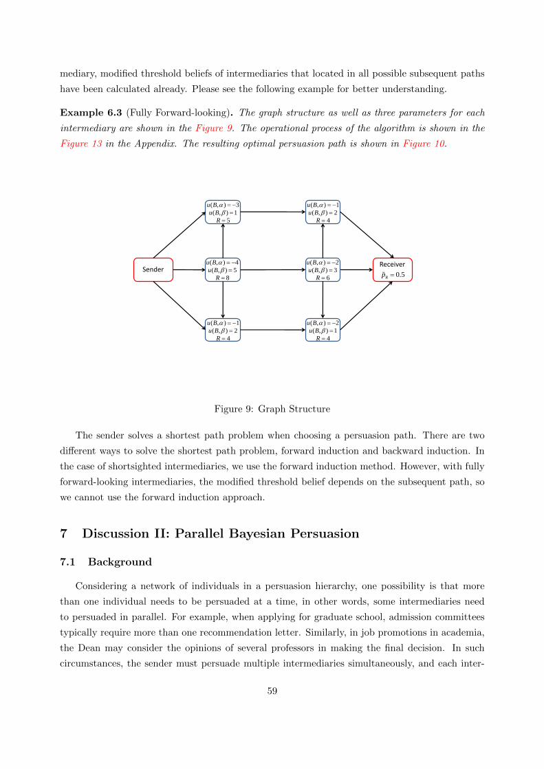
mediary, modified threshold beliefs of intermediaries that located in all possible subsequent paths

have been calculated already. Please see the following example for better understanding.

Example 6.3 (Fully Forward-looking). The graph structure as well as three parameters for each

intermediary are shown in the Figure 9. The operational process of the algorithm is shown in the

Figure 13 in the Appendix. The resulting optimal persuasion path is shown in Figure 10.

Receiver

0.5Rp Sender

( , ) 1

( , ) 2

4

u B

u B

R

( , ) 2

( , ) 1

4

u B

u B

R

( , ) 3

( , ) 1

5

u B

u B

R

( , ) 1

( , ) 2

4

u B

u B

R

( , ) 2

( , ) 3

6

u B

u B

R

( , ) 4

( , ) 5

8

u B

u B

R

Figure 9: Graph Structure

The sender solves a shortest path problem when choosing a persuasion path. There are two

different ways to solve the shortest path problem, forward induction and backward induction. In

the case of shortsighted intermediaries, we use the forward induction method. However, with fully

forward-looking intermediaries, the modified threshold belief depends on the subsequent path, so

we cannot use the forward induction approach.

7 Discussion II: Parallel Bayesian Persuasion

7.1 Background

Considering a network of individuals in a persuasion hierarchy, one possibility is that more

than one individual needs to be persuaded at a time, in other words, some intermediaries need

to persuaded in parallel. For example, when applying for graduate school, admission committees

typically require more than one recommendation letter. Similarly, in job promotions in academia,

the Dean may consider the opinions of several professors in making the final decision. In such

circumstances, the sender must persuade multiple intermediaries simultaneously, and each inter-

59

Receiver

0.5Rp Sender

0.444

0.6

0.554

0.5

0.4570.464

Figure 10: Optimal Persuasion Path

mediary gives their advice to the receiver separately. We begin with the case of one intermediary

per path in a parallel structure, and then generalize to the case of multiple intermediaries in the

parallel structure in Section 7.4.

7.2 Setting

Setup We analyze a parallel Bayesian persuasion setup with one sender and one receiver through

n parallel intermediaries, denoted as j = 1, 2, · · · , n. Binary state, binary action and modified

threshold belief p̃Ij are defined as in previous sections.23 We further assume that the sender

applies public persuasion. In other words, for each signal realization, the incoming beliefs of all

parallel intermediaries are the same under the common prior assumption.

Timeline The parallel persuasion game consists of two stages.

Stage 1: The sender publicly sets up a signal-generating mechanism, which consists of a family

of conditional distributions {π(·|t)}t∈T over a space of signal realizations S, and hence divides the

prior belief into posterior portfolios that satisfy the Bayes’ plausible condition. We denote this

signal as π.

Stage 2: all n intermediaries choose a partition in the lattice structure T×[0, 1] simultaneously,

denoted as π1, · · · , πn.

Our setup is closely related to Gentzkow and Kamenica (2017) [5], which introduces lattice

23There exist slight difference on definition of p̃Ij . Beliefs of intermediaries are correlated using lattcie structurewe introduced later. However, the math formula would not change.

60

structure to multiple senders persuasion. The receiver observes all signals generated by the inter-

mediaries, and hence has partition π ∨ (∨nj=1 πj). The receiver has posterior p with distribution

〈π∨(∨nj=1 πj)〉 and then chooses an action from {A,B}. Their model corresponds nearly identically

to Stage 2.

7.3 Result

Similarly to benchmark model, we can define p̃maxP = max({p̃Ij}j , p̃R) as the minimum modified

threshold belief and p̃minP = min({p̃Ij}j , p̃R) as the maximum modified threshold belief. Again, p̃max

P

quantifies how difficult (B-preferred) sender can persuade the intermediaries. Here, subscript P is

shorted for parallel. By backward induction, we first obtain the following lemma on stage 2.

Lemma 7.1. If some signal realization s induced posterior p such that at least one intermediary

is B-preferred and at least one intermediary is A-preferred, then given signal realization s, the

receiver is eventually fully informed after the persuasions of the intermediaries.

Proof. By contrast we assume the receiver is not fully informed when observing the signal gener-

ating by intermediaries.Then either the B-preferred intermediary or the A-preferred intermediary

will benefit from full disclosure because of the following reason. If for some signal realizations,

some posterior p ∈ (0, 1) is induced, and under this posterior the receiver chooses one action, then

the intermediary that prefers the opposite action will benefit from a full disclosure based on those

signal realizations.

We now move back to stage 1. For the sender, if he passes some posterior p that is inside the

range (p̃minP , p̃max

P ), then the receiver is eventually fully informed. Otherwise, all intermediaries will

reach a consensus and make no further manipulations to the information structure. The following

theorem characterizes the optimal disclosure policy applied by sender, which follows the same

pattern as in the benchmark model, while P subscript denotes parallel persuasion.

Theorem 7.2. The sender’s optimal Bayesian persuasion is (1) no disclosure when p0 ≥ p̃maxP ; (2)

partial disclosure that induces posterior p̃maxP with probability p0

p̃maxP

and 0 with probability 1− p0p̃maxP

.

Proof. Assume the posterior generated by realization s is p, then the utility for the sender is,

u(p) =

0 0 ≤ p < p̃min

P

p p̃minP ≤ p < p̃max

P

1 p̃maxP ≤ p ≤ 1

(31)

61

The concave closure of u(p) is

Cou(p) =

p

p̃maxP

0 ≤ p ≤ p̃maxP

1 p̃maxP ≤ p ≤ 1

(32)

The intuition behind the theorem is quite similar to the benchmark hierarchical model. For

both hierarchical and parallel persuasion, intermediaries preferring different actions is always an

undesirable situation for the sender. Under parallel persuasion, this conflict will finally result in

full disclosure, which is unfavorable. The situation is even worse in hierarchical persuasion. An

A-preferred intermediary will further confound a small probability on β in α, which further lowers

the probability of Pr(d = B). Therefore, following Kamenica and Gentzkow (2011), the sender

tries to generate exactly two posteriors such that one is lowest posterior such that all succeeding

players prefers B at the same time while the other is 0.

7.4 Combining Hierarchical and Parallel Structures

Using the results above, we can extend our result to a more complex general structure: (1)

parallel hierarchical structure and (2) hierarchical parallel structure. Both of them are special

cases of directed acyclic graph that avoid interactions. The following two figures highlight the

network structure, where blue boxes represent intermediaries.

…

…

…

…

Sender Receiver…… …

Figure 11: Parallel Hierarchical Structure

62

Sender Receiver……

Hub Hub…

Figure 12: Hierarchical Parallel Structure

Parallel Hierarchical Bayesian Persuasion

In this scenario, the sender persuades the receiver through n parallel paths, denoted as j =

1, 2, · · · , n. In each path j, there exist mj intermediaries, denoted as kj = 1, 2, · · · ,mj . Binary

state, binary action and modified threshold belief are defined identically to in previous sections.

We let p̃max(j)PH denote the maximum modified threshold belief of path j, and p̃max

PH = maxj p̃max(j)PH .

Consider the academic admissions process. When applying, a student is often asked for support-

ing material such as a recommendation letter from different general categories, such as academics,

sports and arts. For each recommendation letter, student may persuade some reputable individual

in that area indirectly. The admission committee makes a decision based on those three letters.

Hierarchical Parallel Bayesian Persuasion

The sender persuades the receiver through n hubs, denoted as j = 1, 2, · · · , n. Hub j in-

fluences hub j + 1 through mj parallel intermediaries, denoted as kj = 1, 2, · · · ,mj . Binary

state, binary action and modified threshold belief are defined the same as in previous sections.

We let p̃max(j)HP denote the maximum threshold belief connecting hub j and j + 1, and p̃max

HP =

max(maxj p̃max(j)HP ,maxj p̃Ij , p̃R).

In such a network structure, the hubs are more important than intermediaries. Consider the

example of an entry level worker having a profitable idea. During persuasion of the manager,

he may ask several engineers to persuade the manager, who if convinced, persuades his director

through some external experts, and the director may finally persuade the CEO through some

members of board. The manager and director here are the hubs while the engineers and external

experts serve as intermediaries.

63

Corollary 7.3. In both settings described above, the sender’s optimal Bayesian persuasion is (1)

no disclosure when p0 ≥ p̃maxL ; (2) partial disclosure that induces posterior p̃max

L with probabilityp0p̃maxL

and 0 with probability 1 − p0p̃maxL

, where L = PH for the parallel hierarchical structure and

L = HP for the hierarchical parallel structure.

Once again, the results follow the same pattern as the benchmark model. Here we have analyzed

two special cases of directed acyclic graphs. We leave the generalized analysis of directed acyclic

graphs as our future work.

8 Discussion III: Costly Persuasion

8.1 Background

In the Bayesian persuasion literature, we often regard the signal generation process as an

investigation. However, not all signals are costless. The previous approach we used is not generally

feasible if signals are costly. In that case, the sender’s payoff is not fully determined by the

posterior; given the posterior, the payoff also depends on the signal (due to its cost). Since one

cannot express the sender’s payoff as a value function over beliefs, the concavification approach

does not work generally. We need to add some restrictions on form of the cost function to make

it solvable under concavification. By introducing into the hierarchical persuasion model posterior

separable cost functions (Gentzkow and Kamenica, 2014 [27]; Matyskova, 2018), for which the

entropy based cost and residual variance is a typical example, the hierarchical problem is solvable

under concavification.

8.2 Setting

We follow the binary state, binary action and reputation term setup as our benchmark model.

Gentzkow and Kamenica (2014) [27] introduce a family of cost functions that is compatible with the

concavification approach to deriving the optimal signal. Matyskova (2018) uses the same family of

cost functions to analyze a model where the receiver has additional costly information acquisition,

and calls such cost functions posterior separable.

The cost of signals is defined by a measurement of uncertainty H(µ), as a mapping from a

distribution to a real number. Two examples are entropy as proposed by Shannon (1948) and

residual variance (Gentzkow and Kamenica, 2014 [27]). The cost of signals is proportional to the

expected reduction in uncertainty. In our binary setting, without loss of generality, we assume

H(µ) > 0 and H(0) = H(1) = 0. When the probability of state β is p, entropy gives us

HENT(p) = −p ln p− (1− p) ln(1− p) (33)

64

and residual variance gives us

HRES(p) = p(1− p) (34)

Take the prosecution example in Kamenica and Gentzkow (2011) as an example here, at prior

distribution p = 0.3, HENT(p) = 0.611 and HRES(p) = 0.210. If the prosecutor applies a no disclo-

sure policy, then the uncertainty reduction is 0. If prosecutor applies a full disclosure policy, then

the uncertainty measurement for two posteriors are 0 for both measurements and both posteriors.

The uncertainty reduction is 0.611 under entropy and 0.210 under residual variance. Now we

consider the optimal signal, that is the posteriors are 0 with 40 percent and 0.5 with 60 percent.

The uncertainty reductions are given by

HENT(0.3)−(

0.4HENT(0) + 0.6HENT(0.5))

= 0.195

HRES(0.3)−(

0.4HRES(0) + 0.6HRES(0.5))

= 0.060

Then in the persuasion stage, players need to compute the concave closure of the weighted sum-

mation of the raw utility and uncertainty measurement. In the previous section, any intermediary

j tries to maximize the probability of their preferred action being taken by the receiver. However,

when introducing uncertainty, the relative weight of uncertainty which we denote by λ > 0 and the

winning probability may create variation in the net utility of the preferred action. Especially for

an intermediary that is indifferent between two actions, she always applies a no disclosure policy.

Hence, the previous two optimal Bayesian persuasion strategies do not hold generally under costly

persuasion.

8.3 Persuading the Last Intermediary

To obtain a general result, the first difficulty we encounter is that in the persuasion stage, an

intermediary is no longer purely a preferred action maximizer, based on our previous definition.

Since persuasion is costly, each intermediary must take this into consideration. Additionally, we

cannot put the uncertainty measurements directly into the winning probability, we must incorpo-

rate them into the utility terms uj(B,α) and uj(B, β). It is intuitive that when the cost of a signal

is relatively low, the optimal behavior of an intermediary in the persuasion stage is still preferred

action maximization. Here we characterize such a condition.

We first consider the behavior of the last intermediary. For a B-preferred intermediary n, the

utility when inducing belief p to the receiver is0 if p < p̃R

Rn + pun(B, β) + (1− p)un(B,α) if p ≥ p̃R

65

Under Assumption 2.1, when there is no cost, then the optimal policy is partial disclosure that

generates posterior 0 and p̃R when p < p̃R, and no disclosure otherwise. If we incorporate the

uncertainty measure, then concavification is applied on

VBn(p) =

λH(p) if p < p̃R

Rn + pun(B, β) + (1− p)un(B,α) + λH(p) if p ≥ p̃R

The conditions

V ′Bn(0) ≤ VBn(p̃R)− Vn(0)

p̃R

V ′Bn(p̃R) ≤ VBn(p̃R)− Vn(0)

p̃R

are required to keep the optimal policy unchanged: (1) When p < p̃R is still optimal to generate

posteriors 0 and p̃R, and (2) when p ≥ p̃R, no disclosure is still optimal. By re-arranging, we

obtain the following assumption

Assumption 8.1.

Rn ≥ λp̃RH′(0)− p̃Run(B, β)− (1− p̃R)un(B,α)− λH(p̃R)

Rn ≥ −un(B,α) + λ(p̃RH

′(p̃R)−H(p̃R))

for reputation term Rn.

Clearly, entropy based uncertainty measurement never satisfies this assumption becauseH ′(0) =

+∞. The assumption provides us with the lower bound on reputation term conditioning on c and

H(·) such that intermediary n is a preferred action maximizer.

For a A-preferred intermediary n, the utility when inducing belief p to the receiver isRn if p < p̃R

pun(B, β) + (1− p)un(B,α) if p ≥ p̃R

Under Assumption 2.1, when there are no costs, then the optimal policy is disclosure when p < p̃R

and partial disclosure associated with p̃R and 1 otherwise. If we incorporate the uncertainty

measure, then concavification is applied on

VAn(p) =

Rn + λH(p) if p ≤ p̃R

pun(B, β) + (1− p)un(B,α) + λH(p) if p > p̃R

66

We require

V ′An(1) ≥ VAn(1)− VAn(p̃R)

1− p̃R

V ′An(p̃R) ≥ VAn(1)− VAn(p̃R)

1− p̃R

to keep the optimal policy unchanged. By re-arranging, we obtain the following

Assumption 8.2.

Rn ≥ un(B, β)− (1− p̃R)(un(B, β)− un(B,α))− (1− p̃R)H ′(1)λ− λH(p̃R)

Rn ≥ un(B, β)− (1− p̃R)λH ′(p̃R)− λH(p̃R)

for reputation term Rn.

Next, we characterize intermediary n’s choice of A or B in the response stage when the incoming

belief is p. The expected utility for intermediary n of responding with A and B are calculated as

follows,

Un(p|A) =

Rn p ∈ [0, p̃R]

(1−p)(Rn+cH(p̃R)))1−p̃R + (p−p̃R)un(B,β)

1−p̃R − cH(p) p ∈ [p̃R, 1]

Un(p|B) =

pp̃R

(Rn + p̃Run(B, β) + (1− p̃R)un(B,α) + cH(p̃R))− cH(p) p ∈ [0, p̃R]

Rn + un(B,α) + p(un(B, β)− un(B,α)) p ∈ [p̃R, 1]

We need to prove that the modified threshold belief exists uniquely. The boundary conditions are

Un(0|A) = Rn

Un(1|A) = un(B, β)

Un(0|B) = 0

Un(0|B) = Rn + un(B, β)

For p ∈ [0, p̃R],∂2Un(p|B)

∂p2= −λH ′′(p) > 0

For p ∈ [p̃R, 1],∂2Un(p|A)

∂p2= −λH ′′(p) > 0

If Un(p̃R|A) > Un(p̃R|B), then the unique solution exists in [p̃R, 1]. If Un(p̃R|A) < Un(p̃R|B),

then the unique solution exists in [0, p̃R]. Therefore, the modified threshold belief of intermediary

67

n exists uniquely.

8.4 Persuading the Intermediary j

Now we consider the analysis for the general intermediary. Assume that

1. For B-preferred intermediary j, the utility when inducing belief p to intermediary j + 1 is0 if p < p̃maxj

Rj + puj(B, β) + (1− p)uj(B,α) if p ≥ p̃maxj

2. For A-preferred intermediary j, the utility when inducing belief p to intermediary j + 1 isRj if p < p̃minj

puj(B, β) + (1− p)uj(B,α) if p ≥ p̃minj

Similarly, we can write out the lower bound on Rj (similar to previous formulas on the repu-

tation term). In other words, we require reputation term to be large enough. As for the specific

lower bound, the derivation is similar to assumption 8.1 and 8.2) such that in the persuasion stage,

all intermediaries are maximizers of the probability of their preferred action. Now, we consider

the response stage of intermediary j. We characterize intermediary j’s choice of A or B in the

response stage when the incoming belief is p. The expected utility for intermediary j of responding

with A and B are calculated as follows,

Uj(p|A) =

Rj p ∈ [0, p̃minj ]

(1−p)(Rj+λH(p̃minj )))

1−p̃minj

+(p−p̃min

j )uj(B,β)

1−p̃minj

− λH(p) p ∈ [p̃minj , 1]

Uj(p|B) =

p

p̃maxj

(Rj + p̃maxj uj(B, β) + (1− p̃max

j )uj(B,α) + λH(p̃maxj ))− λH(p) p ∈ [0, p̃max

j ]

Rj + uj(B,α) + p(uj(B, β)− uj(B,α)) p ∈ [p̃maxj , 1]

We need to show that an intersection point exists uniquely. In this general case, the boundary

conditions and second order conditions still hold,

Uj(0|A) > Uj(0|B)

Uj(1|A) < Uj(0|B)

∂2Uj(p|A)

∂p2> 0 when p ∈ [p̃min

j , 1]

∂2Uj(p|B)

∂p2> 0 when p ∈ [0, p̃max

j ]

68

Depending on the signs of Uj(p̃minj |A) − Uj(p̃

minj |B) and Uj(p̃

maxj |A) − Uj(p̃

maxj |B), we can

illustrate the uniqueness of the intersection point in three different situations,

1. If Uj(p̃minj |A) > Uj(p̃

minj |B) and Uj(p̃

maxj |A) < Uj(p̃

maxj |B), then the unique solution exists

in [p̃minj , p̃max

j ].

2. If Uj(p̃minj |A) < Uj(p̃

minj |B), then the unique solution exists in [0, p̃min

j ].

3. If Uj(p̃maxj |A) > Uj(p̃

maxj |B), then the unique solution exists in [p̃max

j , 1].

Therefore, the modified threshold belief of intermediary j exists uniquely.

The equilibrium strategies of intermediaries in the case of costly persuasion share the same

pattern with benchmark model: a threshold policy in the response stage and similar disclosure

policy as described in Theorem 2.5. In order for costly persuasion to share the same pattern as

benchmark model, we need to guarantee (1) the objective in the persuasion stage is preferred

action maximization, and (2) the modified threshold belief exists uniquely. For the first condition,

a costly signal requires a higher lower bound for the reputation term. As the cost level λ increases,

the lower bound of the reputation term needed increases. However, for the second condition, there

are no additional requirements for parameters except for the concavity of H(·).

9 Conclusion

Situations where individuals must be convinced through a chain of command are abundant

in many formal application procedures and bureaucracies. In this paper we analyze Bayesian

persuasion in a hierarchical setting, in which a sender persuades a receiver through a series of

intermediaries. By introducing reputation considerations of the intermediaries in the chain, we

solve for the equilibrium persuasion strategies, and identify two intuitive hierarchical persuasion

approaches out of the multiplicity of equilbria: focusing on persuading the immediately subsequent

intermediary, and focusing on persuading the most difficult to convince along the hierarchy. In

each of our extensions, we examine whether these intuitive strategies are sustained as equilibrium

persuasion approaches. It is worth noting that although the hierarchical Bayesian persuasion

game has multiple equilbria, these equilibria are payoff equivalent, which pins down the payoff-

based prediction power of the model. By studying parameters’ influence on modified threshld

belief, we find out that adding another easy convincible intermediary may be beneficial for sender.

What’s more, we characterize the optimal ordering of intermediaries for sender, which provides

the insight when seeking consensus of agents through a persuasion chain.

Three main extensions of the benchmark model are considered. First, a natural extension is

to incorporate the presence of private information among the intermediaries, which we capture by

an uncertainty by other players about an intermediary’s persuadability. The private information

setting favors the strategy of persuading the immediately subsequent intermediary over persuad-

ing the most difficult to persuade player in this setting. Our second extension seeks to justify

69

the reputation concern in the benchmark model, by showing that such reputation concern arises

naturally in a repeated sequential persuasion setting. The third extension we consider is that any

intermediary has the option to break the chain of persuasion by declining to send any message. The

influence of this outside option of the intermediaries can be severe, as all preceding intermediaries

who gave messages may incur large costs when someone takes the outside option, thus drawing

similarities to the herding literature in terms of intermediaries decisions to send messages at all.

Three minor extensions or discussions of the model are also considered, mainly allowing the

sender to choose among different potential persuasion paths, allowing for parallel persuasion in

the hierarchy, and incorporating the possibility of costly persuasion. These analyses provide a

framework for analyzing these intuitive extensions of the main model of Bayesian persuasion in a

hierarchical setting.

70

A Discussion of the Role of the Reputation Term Rj

The utility for intermediary j when the response is r ∈ {A,B}, the final decision is d ∈ {A,B}and the state is T ∈ {α, β}, is defined as

RjI(r = d) + uj(d, t) (35)

Intermediary j maximizes the probability of his or her preferred action if and only if interme-

diary j prefers his or her preferred action for all possible posteriors p ∈ [0, 1],

∀r, ∀p,Rj + puj(r, β) + (1− p)uj(r, α) ≥ puj(−r, β) + (1− p)uj(−r, α) (36)

where −r =

A r = B

B r = A. This equation is further equivalent to:

∀r, ∀t, Rj + uj(r, t) ≥ uj(−r, t) (37)

Otherwise, intermediary j prefers A at state α and prefers B at state β, which makes full disclosure

the best strategy.

If preferred action of intermediary j is A, then, it is required that

Rj + uj(A,α) ≥ uj(B,α)

Rj + uj(A, β) ≥ uj(B, β)

The first equation holds because uj(B,α) < uj(A,α). The second equation implies Rj > uj(B, β).

If preferred action of intermediary j is B, then, it is required that

Rj + uj(B,α) ≥ uj(A,α)

Rj + uj(B, β) ≥ uj(A, β)

The second equation holds because uj(B, β) > uj(A, β). The first equation impliesRj > −uj(B,α).

Therefore, we need Assumption 2.1.

71

B Graphical Illustration of 6 Cases of Theorem 2.5

Case (1): B-preferred, p̃I,k+1 < p̃mink+1 < p̃max

k+1.

max

1kp

1

10 min

1kp , 1I kp

max

1kp

1

10 min

1kp , 1I kp

Case (2): A-preferred, p̃I,k+1 < p̃mink+1 < p̃max

k+1

1

10 , 1I kp max

1kp min

1kp

1

10 , 1I kp max

1kp min

1kp

72

Case (3): B-preferred, p̃mink+1 < p̃I,k+1 < p̃max

k+1

1

10 min

1kp , 1I kp

max

1kp

1

10 , 1I kp max

1kp min

1kp

Case (4): A-preferred, p̃mink+1 < p̃I,k+1 < p̃max

k+1

1

10 , 1I kp max

1kp min

1kp

1

10 , 1I kp max

1kp min

1kp

Case (5): B-preferred, p̃mink+1 < p̃max

k+1 < p̃I,k+1

1

10 , 1I kp min

1kp max

1kp

1

10 , 1I kp min

1kp max

1kp

73

Case (6): A-preferred, p̃mink+1 < p̃max

k+1 < p̃I,k+1

1

10 , 1I kp min

1kp max

1kp max

1kp

1

10 , 1I kp min

1kp

74

C Comparison Between p̃j and p̃Ij

Since p̃j is defined by uj(B,α) and uj(B, β):

p̃j =−uj(B,α)

uj(B, β)− uj(B,α)(38)

At the same time, the modified threshold belief is solved by

Uj(p|A) = Uj(p|B) (39)

where

Uj(p|A) =

Rj p ∈ [0, p̃minj ]

1−p1−p̃min

jRj +

p−p̃minj

1−p̃minjuj(B, β) p ∈ [p̃min

j , 1]

Uj(p|B) =

p

p̃maxj

(Rj + uj(B,α)) + p(uj(B, β)− uj(B,α)) p ∈ [0, p̃maxj ]

Rj + uj(B,α) + p(uj(B, β)− uj(B,α)) p ∈ [p̃maxj , 1]

If we plug p̃j into above two equations, we will have

Uj(p̃j |A) =

Rj p̃j ∈ [0, p̃minj ]

1−p̃j1−p̃min

jRj +

p̃j−p̃minj

1−p̃minj

uj(B, β) p̃j ∈ [p̃minj , 1]

Uj(p̃j |B) =

p̃jp̃maxj

(Rj + uj(B,α))− uj(B,α) p̃j ∈ [0, p̃maxj ]

Rj p̃j ∈ [p̃maxj , 1]

p̃Ij < p̃j is equivalent to

Uj(p̃j |B) > Uj(p̃j |A) (40)

because p̃Ij solves Uj(p|B) = Uj(p|A) and Uj(p|B) (Uj(p|A)) is increasing (decreasing).

From now on, we set A = −uj(B,α),B = uj(B, β).

Case (1) When p̃j ≤ p̃minj , p̃Ij > p̃j :

Uj(p̃j |B)− Uj(p̃j |A)

=A/(A + B)

p̃maxj

(Rj − A) + A−Rj

=A/(A + B)− p̃max

j

p̃maxj

(Rj − A)

=p̃j − p̃max

j

p̃maxj

(Rj − A)

<0

(41)

75

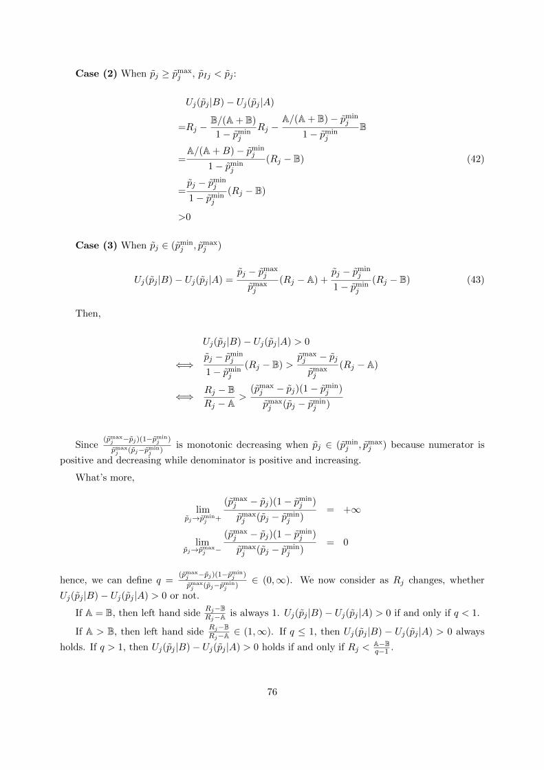
Case (2) When p̃j ≥ p̃maxj , p̃Ij < p̃j :

Uj(p̃j |B)− Uj(p̃j |A)

=Rj −B/(A + B)

1− p̃minj

Rj −A/(A + B)− p̃min

j

1− p̃minj

B

=A/(A +B)− p̃min

j

1− p̃minj

(Rj − B)

=p̃j − p̃min

j

1− p̃minj

(Rj − B)

>0

(42)

Case (3) When p̃j ∈ (p̃minj , p̃max

j )

Uj(p̃j |B)− Uj(p̃j |A) =p̃j − p̃max

j

p̃maxj

(Rj − A) +p̃j − p̃min

j

1− p̃minj

(Rj − B) (43)

Then,

Uj(p̃j |B)− Uj(p̃j |A) > 0

⇐⇒p̃j − p̃min

j

1− p̃minj

(Rj − B) >p̃maxj − p̃jp̃maxj

(Rj − A)

⇐⇒ Rj − BRj − A

>(p̃maxj − p̃j)(1− p̃min

j )

p̃maxj (p̃j − p̃min

j )

Since(p̃maxj −p̃j)(1−p̃min

j )

p̃maxj (p̃j−p̃min

j )is monotonic decreasing when p̃j ∈ (p̃min

j , p̃maxj ) because numerator is

positive and decreasing while denominator is positive and increasing.

What’s more,

limp̃j→p̃min

j +

(p̃maxj − p̃j)(1− p̃min

j )

p̃maxj (p̃j − p̃min

j )= +∞

limp̃j→p̃max

j −

(p̃maxj − p̃j)(1− p̃min

j )

p̃maxj (p̃j − p̃min

j )= 0

hence, we can define q =(p̃maxj −p̃j)(1−p̃min

j )

p̃maxj (p̃j−p̃min

j )∈ (0,∞). We now consider as Rj changes, whether

Uj(p̃j |B)− Uj(p̃j |A) > 0 or not.

If A = B, then left hand sideRj−BRj−A is always 1. Uj(p̃j |B)− Uj(p̃j |A) > 0 if and only if q < 1.

If A > B, then left hand sideRj−BRj−A ∈ (1,∞). If q ≤ 1, then Uj(p̃j |B) − Uj(p̃j |A) > 0 always

holds. If q > 1, then Uj(p̃j |B)− Uj(p̃j |A) > 0 holds if and only if Rj <A−Bq−1 .

76

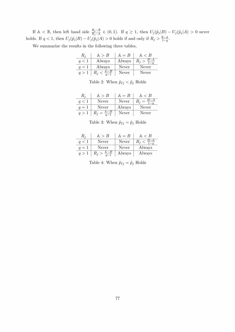
If A < B, then left hand sideRj−BRj−A ∈ (0, 1). If q ≥ 1, then Uj(p̃j |B) − Uj(p̃j |A) > 0 never

holds. If q < 1, then Uj(p̃j |B)− Uj(p̃j |A) > 0 holds if and only if Rj >B−A1−q .

We summarize the results in the following three tables,

Rj A > B A = B A < B

q < 1 Always Always Rj >B−A1−q

q = 1 Always Never Never

q > 1 Rj <A−Bq−1 Never Never

Table 2: When p̃Ij < p̃j Holds

Rj A > B A = B A < B

q < 1 Never Never Rj = B−A1−q

q = 1 Never Always Never

q > 1 Rj = A−Bq−1 Never Never

Table 3: When p̃Ij = p̃j Holds

Rj A > B A = B A < B

q < 1 Never Never Rj <B−A1−q

q = 1 Never Never Always

q > 1 Rj >A−Bq−1 Always Always

Table 4: When p̃Ij = p̃j Holds

77

D Details about Persuading the Intermediary j

We first define the expected utility for intermediary j with the following features

1. Responding A/B to intermediary j − 1

2. Intermediary j generates posterior p to the Intermediary j + 1.

3. Type of intermediary j is θj

4. Type of intermediary j + 1 is θj+1

by the expressions

Uj(p|A, θj , θj+1) = (1− Ij+1(p|θj+1))Rj + Ij+1(p|θj+1)(puj(B, β|θj) + (1− p)uj(B,α|θj))

Uj(p|B, θj , θj+1) = Ij+1(p|θj+1)(Rj + puj(B, β|θj) + (1− p)uj(B,α|θj))

respectively, where boolean variable Ij+1(p|θj+1) = I(p̃I,j+1(θj+1) ≤ p) ∈ {0, 1} represents whether

receiver will choose action B or not when intermediary j passes posterior p to intermediary j + 1.

Firstly, it is easy to see that Uj(p|B, θj , θj+1) is increasing in p because when p increases, both

Ij+1(p|θj+1) and Rj + puj(B, β|θj) + (1− p)uj(B,α|θj) are nonnegative and increasing. Secondly,

we have the following boundary values, which help us prove the existence and uniqueness of the

modified threshold belief.

Uj(0|A, θj , θj+1) = Rj

Uj(1|A, θj , θj+1) = uj(B, β)

Uj(0|B, θj , θj+1) = 0

Uj(1|B, θj , θj+1) = Rj + uj(B, β)

In addition, we have Uj(p|A, θj , θj+1) ≤ Rj − Ij+1(p|θj+1)(Rj − uj(B, β)) ≤ Rj . Therefore, if

we take the expectation over θj+1, we have the expected utility for A-preferred and B-preferred

intermediaries j given his type is θj under two extreme posteriors (0 and 1),

Eθj+1[Uj(0|A, θj , θj+1)] = Rj

Eθj+1[Uj(1|A, θj , θj+1)] = uj(B, β)

Eθj+1[Uj(0|B, θj , θj+1)] = 0

Eθj+1[Uj(1|B, θj , θj+1)] = Rj + uj(B, β)

Then by Bayesian persuasion, for an A-preferred player, the best he can achieve is the concave

closure of Eθj+1[Uj(0|A, θj , θj+1)], Co(Eθj+1

[Uj(p|A, θj , θj+1)]); for B-preferred player, the best he

78

can achieve is the concave closure of Eθj+1[Uj(0|B, θj , θj+1)], Co(Eθj+1

[Uj(p|B, θj , θj+1)]). We then

need to compared whether response A or B is better.

By similar demonstration as persuading last intermediary, Co(Eθj+1[Uj(p|A, θj , θj+1)]) is de-

creasing in p while Co(Eθj+1[Uj(p|B, θj , θj+1)]) is increasing in p. Therefore, single crossing prop-

erty still holds.

Lemma D.1. Co(Eθj+1[Uj(p|A, θj , θj+1)]) = Co(Eθj+1

[Uj(p|B, θj , θj+1)]) has unique solution p =

p̃Ij(θj).

Hence, there exists a threshold value p̃Ij(θj) for type θj , called modified threshold belief such

that intermediary j is indifferent between choosing A and B in response stage.

79

E Graphical Illustration of 12 Cases of Theorem 5.2

Intermediary k avoids to induce any posterior between p̃Ak+1 and p̃Bk+1.

Case (1): B-preferred, p̃Ak+1 < p̃Bk+1 < p̃mink+1 < p̃max

k+1.

max

1kp

1

10 min

1kp

1

A

kp

1

B

kp max

1kp

1

10 min

1kp

1

A

kp

1

B

kp

Case (2): A-preferred, p̃Ak+1 < p̃Bk+1 < p̃mink+1 < p̃max

k+1

max

1kp

1

10 min

1kp

1

A

kp

1

B

kp max

1kp

1

10 min

1kp

1

A

kp

1

B

kp

80

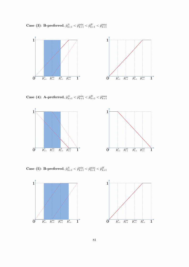
Case (3): B-preferred, p̃Ak+1 < p̃mink+1 < p̃Bk+1 < p̃max

k+1

max

1kp

1

10 min

1kp

1

A

kp

1

B

kp max

1kp

1

10 1

A

kp min

1kp

1

B

kp

Case (4): A-preferred, p̃Ak+1 < p̃mink+1 < p̃Bk+1 < p̃max

k+1

max

1kp

1

10 min

1kp

1

A

kp

1

B

kp max

1kp

1

10 min

1kp

1

A

kp

1

B

kp

Case (5): B-preferred, p̃Ak+1 < p̃mink+1 < p̃max

k+1 < p̃Bk+1

max

1kp

1

10 min

1kp

1

A

kp

1

B

kp max

1kp

1

10 min

1kp

1

A

kp

1

B

kp

81

Case (6): A-preferred, p̃Ak+1 < p̃mink+1 < p̃max

k+1 < p̃Bk+1

max

1kp

1

10 min

1kp

1

A

kp

1

B

kp max

1kp

1

10 min

1kp

1

A

kp

1

B

kp

Case (7): B-preferred, p̃mink+1 < p̃Ak+1 < p̃Bk+1 < p̃max

k+1.

max

1kp

1

10 min

1kp

1

A

kp

1

B

kp max

1kp

1

10 min

1kp

1

A

kp

1

B

kp

Case (8): A-preferred, p̃mink+1 < p̃Ak+1 < p̃Bk+1 < p̃max

k+1

max

1kp

1

10 min

1kp

1

A

kp

1

B

kp max

1kp

1

10 min

1kp

1

A

kp

1

B

kp

82

Case (9): B-preferred, p̃mink+1 < p̃Ak+1 < p̃max

k+1 < p̃Bk+1

max

1kp

1

10 min

1kp

1

A

kp

1

B

kp max

1kp

1

10 min

1kp

1

A

kp

1

B

kp

Case (10): A-preferred, p̃mink+1 < p̃Ak+1 < p̃max

k+1 < p̃Bk+1

max

1kp

1

10 min

1kp

1

A

kp

1

B

kp max

1kp

1

10 min

1kp

1

A

kp

1

B

kp

Case (11): B-preferred, p̃mink+1 < p̃max

k+1 < p̃Ak+1 < p̃Bk+1

max

1kp

1

10 min

1kp

1

A

kp

1

B

kp max

1kp

1

10 min

1kp

1

A

kp

1

B

kp

83

Case (12): A-preferred, p̃mink+1 < p̃max

k+1 < p̃Ak+1 < p̃Bk+1

max

1kp

1

10 min

1kp

1

A

kp

1

B

kp max

1kp

1

10 min

1kp

1

A

kp

1

B

kp

84

F Details about Dijkstra’s Algorithm

Introduction Dijkstra’s algorithm is an algorithm for finding the shortest paths between nodes

in a graph. This algorithm was proposed by computer scientist Edsger W. Dijkstra in 1956 and

published three years later. For a given source node in the graph, the algorithm iteratively finds

the shortest path between that node and every other. Hence, by stopping the algorithm once

the shortest path to the destination node has been reached, the algorithm finds the shortest path

between s (sender node) and r (receiver node).

Distance However, the definition of distance is different from the standard framework in shortest

path problem. For a directed graph G = (V,E), we define the distance from s to v through one

path as the maximum modified threshold believes of nodes that involved in such path. The proof

of correctness are inductive.

Hypothesis For each node v ∈ Q, φ(v) is considered the minimax (modified) threshold belief

from s to v; and for each unvisited node u, φ(u) is assumed the minimax (modified) threshold

belief from s to u when traveling via visited nodes only. This assumption is only considered if a

path exists, otherwise the distance is set to infinity.

Base Case When there is just one visited node, namely the initial node s, in which case the

hypothesis is trivial.

Induction Assume the hypothesis for n − 1 visited nodes. In which case, we choose an edge

(v, u) where u has the least φ(u) (Line 8-10) of any unvisited nodes and the edge (v, u) is such

that φ(u) = max(φ(v), p̃(u)) (Line 6). φ(u) is considered to be the minimax (modified) threshold

belief from s to u because if there were a path with shorter path, and if w was the first unvisited

node on that path then by the original hypothesis φ(w) > φ(u) which creates a contradiction.

Similarly if there was a shorter path to u without using unvisited nodes, and if the last but one

node on that path were w, then we would have had φ(u) = max(φ(w), p̃(u)), also a contradiction.

After processing u it will still be true that for each unvisited nodes w, φ(w) will be the shortest

distance from s to w using visited nodes only, because if there were a shorter path that doesn’t go

by u we would have found it previously, and if there were a shorter path using u we would have

updated it when processing u.

Running Algorithm

85

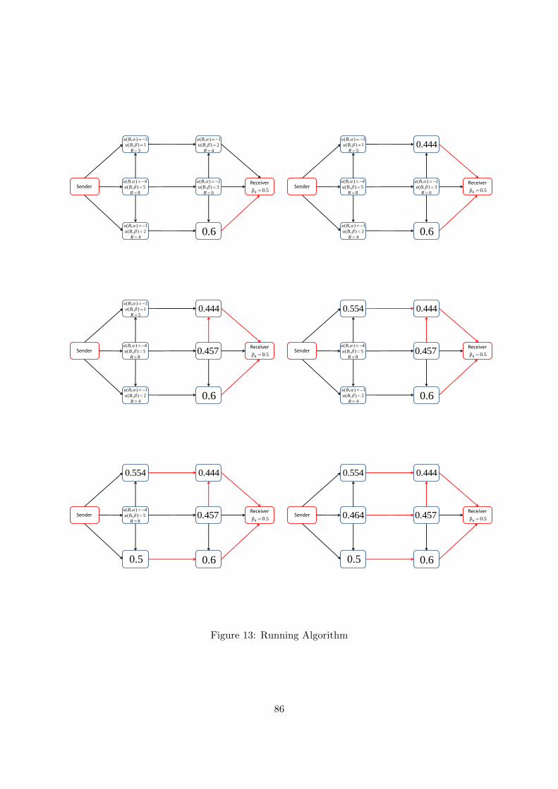
Receiver

0.5Rp Sender

( , ) 1

( , ) 2

4

u B

u B

R

0.6

( , ) 3

( , ) 1

5

u B

u B

R

( , ) 1

( , ) 2

4

u B

u B

R

( , ) 2

( , ) 3

6

u B

u B

R

( , ) 4

( , ) 5

8

u B

u B

R

Receiver

0.5Rp Sender

0.444

0.6

( , ) 3

( , ) 1

5

u B

u B

R

( , ) 1

( , ) 2

4

u B

u B

R

( , ) 2

( , ) 3

6

u B

u B

R

( , ) 4

( , ) 5

8

u B

u B

R

Receiver

0.5Rp Sender

0.444

0.6

( , ) 3

( , ) 1

5

u B

u B

R

( , ) 1

( , ) 2

4

u B

u B

R

0.457( , ) 4

( , ) 5

8

u B

u B

R

Receiver

0.5Rp Sender

0.444

0.6

0.554

( , ) 1

( , ) 2

4

u B

u B

R

0.457( , ) 4

( , ) 5

8

u B

u B

R

Receiver

0.5Rp Sender

0.444

0.6

0.554

0.5

0.457( , ) 4

( , ) 5

8

u B

u B

R

Receiver

0.5Rp Sender

0.444

0.6

0.554

0.5

0.4570.464

Figure 13: Running Algorithm

86

References

[1] E. Kamenica and M. Gentzkow, “Bayesian persuasion,” American Economic Review, vol. 101,

no. 6, pp. 2590–2615, 2011.

[2] D. Bergemann and S. Morris, “Information design: A unified perspective,” Journal of Eco-

nomic Literature, vol. 57, no. 1, pp. 44–95, 2019.

[3] E. Kamenica, “Bayesian persuasion and information design,” Annual Review of Economics,

vol. forthcoming, 2019.

[4] F. Li and P. Norman, “Sequential persuasion,” Working Paper, 2018.

[5] M. Gentzkow and E. Kamenica, “Bayesian persuasion with multiple senders and rich signal

spaces,” Games & Economic Behavior, vol. 104, 2017.

[6] M. Gentzkow and E. Kamenica, “Competition in persuasion,” Review of Economic Studies,

vol. 84, pp. 300–322, 2017.

[7] R. Alonso and O. Camara, “Bayesian persuasion with heterogeneous priors,” Journal of Eco-

nomic Theory, vol. 165, pp. 672–706, 2016.

[8] R. Alonso and O. Camara, “Persuading voters,” American Economic Review, vol. 106, no. 11,

pp. 3590–3605, 2016.

[9] A. Bardhi and Y. Guo, “Modes of persuasion toward unanimous consent,” Theoretical Eco-

nomics, vol. 13, no. 3, pp. 1111–1150, 2018.

[10] J. Chan, S. Gupta, F. Li, and Y. Wang, “Pivotal persuasion,” Journal of Economic Theory,

vol. 180, pp. 178–202, 2019.

[11] Y. Wang, “Bayesian persuasion with multiple receivers,” Working Paper, 2015.

[12] L. Marie and R. Ludovic, “Public persuasion,” Working Paper, 2016.

[13] S. Board and J. Lu, “Competitive information disclosure in search markets,” Journal of

Political Economy, vol. 126, no. 5, pp. 1965–2010, 2018.

[14] F. Wu and J. Zheng, “Double directional persuasion,” Working Paper, 2019.

[15] K. Andrew, “Mediated persuasion,” Working Paper, 2018.

[16] Y. Qian, “Persuasion through a strategic moderator,” Working Paper, 2019.

[17] J. C. Ely, “Beeps,” American Economic Review, vol. 107, no. 1, pp. 31–53, 2017.

[18] J. Ely, A. Frankel, and E. Kamenica, “Suspense and surprise,” Journal of Political Economy,

vol. 123, no. 1, pp. 215–260, 2015.

87

[19] J. Ely and M. Szydlowski, “Moving the goalposts,” Journal of Political Economy, vol. forth-

coming, 2019.

[20] M. Felgenhauer and P. Loerke, “Bayesian persuasion with private experimentation,” Interna-

tional Economic Review, vol. 58, no. 3, pp. 829–856, 2017.

[21] V. P. Crawford and J. Sobel, “Strategic information transmission,” Econometrica, vol. 50,

no. 6, pp. 1431–1451, 1982.

[22] M. Ivanov, “Communication via a strategic mediator,” Journal of Economic Theory, vol. 145,

no. 2, pp. 869–884, 2010.

[23] A. Ambrus, E. M. Azevedo, and Y. Kamada, “Hierarchical cheap talk,” Theoretical Eco-

nomics, vol. 8, no. 1, pp. 233–261, 2013.

[24] A. Kolotilin, T. Mylovanov, A. Zapechelnyuk, and L. Ming, “Persuasion of a privately in-

formed receiver,” Econometrica, vol. 85, no. 6, pp. 1949–1964, 2017.

[25] A. Kolotilin, “Optimal information disclosure: A linear programming approach,” Theoretical

Economics, vol. 13, no. 2, pp. 607–635, 2018.

[26] B. James and Q. Daniel, “Persuasion for the long run,” Journal of Political Economy,

vol. forthcoming, 2019.

[27] M. Gentzkow and E. Kamenica, “Costly persuasion,” American Economic Review, vol. 104,

no. 5, pp. 457–462, 2014.

[28] R. Hodler, S. Loertscher, and D. Rohner, “Persuasion, binary choice, and the costs of dishon-

esty,” Economics Letters, vol. 124, no. 2, pp. 195–198, 2014.

[29] D. P. Berksekas, Dynamic Programming and Optimal Control, Volume II. Athena Scientific,

2012.

[30] S. Bikhchandani, D. Hirshleifer, and I. Welch, “A theory of fads, fashion, custom, and cultural

change as informational cascades,” Journal of Political Economy, vol. 100, no. 5, pp. 992–1026,

1992.

88