Hidden Markov Models

Modified from:http://www.cs.iastate.edu/~cs544/Lectures/lectures.html

Nucleotide frequencies in the human genome

A C T G

29.5 20.4 20.5 29.6

CpG Islands • CpG dinucleotides are rarer than would be expected

from the independent probabilities of C and G. – Reason: When CpG occurs, C is typically chemically modified

by methylation and there is a relatively high chance of methyl-C mutating into T

• High CpG frequency may be biologically significant; e.g., may signal promoter region (“start” of a gene).

• A CpG island is a region where CpG dinucleotides are much more abundant than elsewhere.

Written CpG to distinguish from a C≡G base pair)

Hidden Markov Models

• Components: – Observed variables

• Emitted symbols – Hidden variables – Relationships between them

• Represented by a graph with transition probabilities

• Goal: Find the most likely explanation for the observed variables

The occasionally dishonest casino

• A casino uses a fair die most of the time, but occasionally switches to a loaded one – Fair die: Prob(1) = Prob(2) = . . . = Prob(6) = 1/6 – Loaded die: Prob(1) = Prob(2) = . . . = Prob(5) = 1/10,

Prob(6) = ½ – These are the emission probabilities

• Transition probabilities – Prob(Fair → Loaded) = 0.01 – Prob(Loaded → Fair) = 0.2 – Transitions between states obey a Markov process

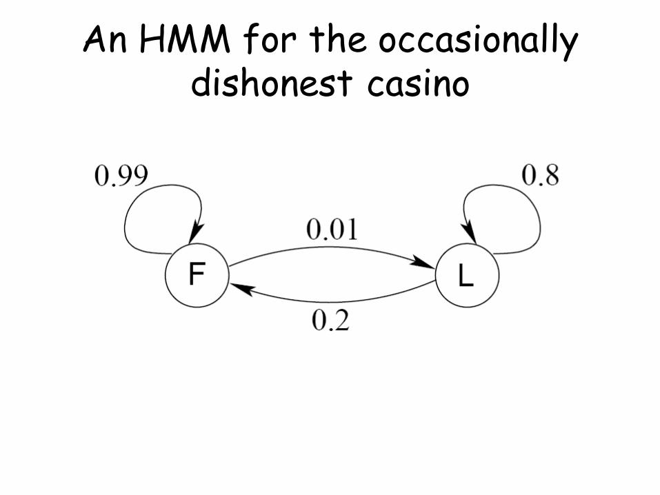
An HMM for the occasionally dishonest casino

0.99 0.8

0.2

0.01

The occasionally dishonest casino • Known:

– The structure of the model – The transition probabilities

• Hidden: What the casino did – FFFFFLLLLLLLFFFF...

• Observable: The series of die tosses – 3415256664666153...

• What we must infer: – When was a fair die used? – When was a loaded one used?

• The answer is a sequence FFFFFFFLLLLLLFFF...

Making the inference • Model assigns a probability to each explanation of the

observation: P(326|FFL) = P(3|F)·P(F→F)·P(2|F)·P(F→L)·P(6|L) = 1/6 · 0.99 · 1/6 · 0.01 · ½

• Maximum Likelihood: Determine which explanation is most likely – Find the path most likely to have produced the observed

sequence • Total probability: Determine probability that observed

sequence was produced by the HMM – Consider all paths that could have produced the observed

sequence

Notation • x is the sequence of symbols emitted by model

– xi is the symbol emitted at time i • A path, π, is a sequence of states

– The i-th state in π is πi • akr is the probability of making a transition from

state k to state r:

• ek(b) is the probability that symbol b is emitted when in state k

)|Pr( 1 kra iikr === −ππ

)|Pr()( kbxbe iik === π

A “parse” of a sequence 1

2

K

…

1

2

K

…

1

2

K

…

…

…

…

1

2

K

…

x1 x2 x3 xL

2

1

K

2

∏=

+⋅=

L

ii iii

axeax1

0 11)(),Pr( πππππ

0 0

The occasionally dishonest casino

00227.06199.0

6199.0

615.0

)6()2()6(),Pr( 0)1(

≈

×××××=

= FFFFFFFF eaeaeax π

008.05.08.01.08.05.05.0

)6()2()6(),Pr( 0)2(

=

×××××=

= LLLLLLLL eaeaeax π

0000417.0

5.001.0612.05.05.0

)6()2()6(),Pr( 00)3(

≈

×××××=

= LLFLFLFLL aeaeaeax π

FFF=)1(π

LLL=)2(π

LFL=)3(π

6,2,6,, 321 == xxxx

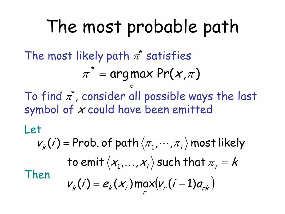
The most probable path The most likely path π* satisfies

),Pr(maxarg* πππ

x=

To find π*, consider all possible ways the last symbol of x could have been emitted

( )rkrrikk aivxeiv )1(max)()( −=

Let

Then kxx

iv

ii

ik

=

=

π

ππ

that such ,, emit to likely most ,, path of Prob.)(

1

1

The Viterbi Algorithm • Initialization (i = 0)

• Recursion (i = 1, . . . , L): For each state k

• Termination:

( )rkrrikk aivxeiv )1(max)()( −=

( )0* )(max),Pr( kkk

aLvx =π

0 for 0)0( ,1)0(0 >== kvv k

To find π*, use trace-back, as in dynamic programming

Viterbi: Example

1

π

x

0

0

6 2 6 ε

(1/6)×(1/2) = 1/12

0

(1/2)×(1/2) = 1/4

(1/6)×max{(1/12)×0.99, (1/4)×0.2} = 0.01375

(1/10)×max{(1/12)×0.01, (1/4)×0.8} = 0.02

B

F

L

0 0

(1/6)×max{0.01375×0.99, 0.02×0.2} = 0.00226875

(1/2)×max{0.01375×0.01, 0.02×0.8} = 0.08

( )rkrrikk aivxeiv )1(max)()( −=

Viterbi gets it right more often than not

An HMM for CpG islands

Emission probabilities are 0 or 1. E.g. eG-(G) = 1, eG-(T) = 0

See Durbin et al., Biological Sequence Analysis,. Cambridge 1998

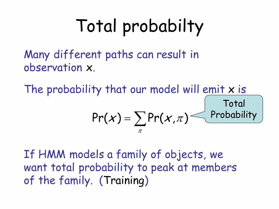
Total probabilty Many different paths can result in observation x.

∑=π

π ),Pr()Pr( xx

The probability that our model will emit x is Total

Probability

If HMM models a family of objects, we want total probability to peak at members of the family. (Training)

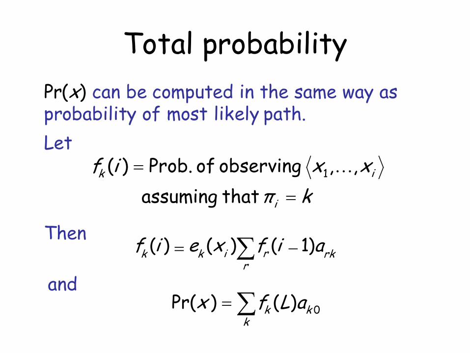
Total probability

Let

Then

that assuming ,, observing of Prob.)( 1

kπxxif

i

ik

=

=

∑ − = r

rk r i k k a i f x e i f ) 1 ( ) ( ) (

∑=k

kk aLfx 0)()Pr(

Pr(x) can be computed in the same way as probability of most likely path.

and

The Forward Algorithm • Initialization (i = 0)

• Recursion (i = 1, . . . , L): For each state k

• Termination:

∑ −=r

rkrikk aifxeif )1()()(

∑=k

kk aLfx 0)()Pr(

0 for 0)0( ,1)0(0 >== kff k

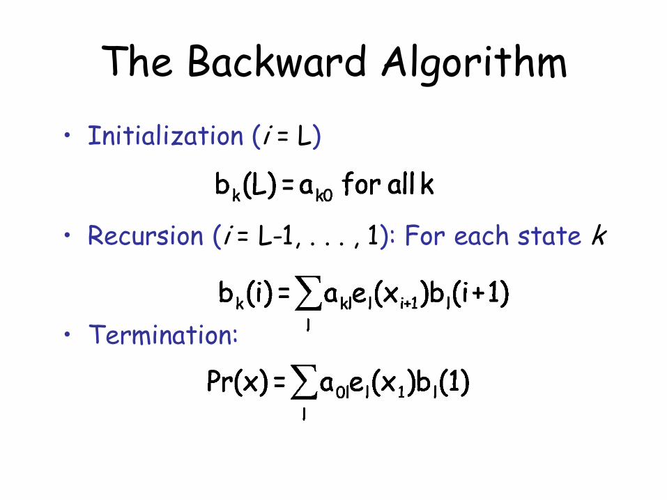
The Backward Algorithm • Initialization (i = L)

• Recursion (i = L-1, . . . , 1): For each state k

• Termination:

Posterior Decoding • How likely is it that my observation comes

from a certain state?

• Like the Forward matrix, one can compute a Backward matrix

• Multiply Forward and Backward entries

– P(x) is the total probability computed by, e.g., forward algorithm

Posterior Decoding

With prob 0.01 for switching to the loaded die:

With prob 0.05 for switching to the loaded die:

Estimating the probabilities (“training”)

• Baum-Welch algorithm – Start with initial guess at transition probabilities – Refine guess to improve the total probability of the training

data in each step • May get stuck at local optimum

– Special case of expectation-maximization (EM) algorithm • Viterbi training

– Derive probable paths for training data using Viterbi algorithm

– Re-estimate transition probabilities based on Viterbi path – Iterate until paths stop changing

Profile HMMs • Model a family of sequences • Derived from a multiple alignment of the

family • Transition and emission probabilities are

position-specific • Set parameters of model so that total

probability peaks at members of family • Sequences can be tested for membership in

family using Viterbi algorithm to match against profile

Profile HMMs

Profile HMMs: Example

Source: http://www.csit.fsu.edu/~swofford/bioinformatics_spring05/

Note: These sequences could lead to other paths.

Pfam • “A comprehensive collection of protein

domains and families, with a range of well-established uses including genome annotation.”

• Each family is represented by two multiple sequence alignments and two profile-Hidden Markov Models (profile-HMMs).

• A. Bateman et al. Nucleic Acids Research (2004) Database Issue 32:D138-D141

Lab 5 I1 I2 I3 I4

D1 D2 D3

M1 M2 M3

Some recurrences

)()()()1()()(

)1()1(

max)()(

111

111

111

1

11

ivaeivivaxeiv

ivaiva

xeiv

BBDDD

BBIiII

IMI

BBMiMM

⋅⋅−=

−⋅⋅=

−⋅−⋅

⋅=

I1 I2 I3 I4

D1 D2 D3

M1 M2 M3

More recurrences

)()()()1()()(

)1()1()1(

max)()(

12122

12122

121

121

222

22

ivaeivivaxeiv

ivaivaiva

xeiv

MDMDD

MIMiII

DMD

MMM

IMI

iMM

⋅⋅−=

−⋅⋅=

−⋅−⋅−⋅

⋅=

I1 I2 I3 I4

D1 D2 D3

M1 M2 M3

ε T A G ε Begin 1 0 0 0 0

M1 0 0.35 M2 0 0.04 M3 0 0 I1 0 0.025 I2 0 0 I3 0 0 I4 0 0 D1 0.2 0 D2 0 0.07 D3 0 0

End 0 0