hermite-hadamard inequality in the geometry of banach spaces
TRANSCRIPT

Hermite-Hadamard Inequality inthe Geometry of Banach Spaces
Eder Kikianty
This thesis is presented in fulfilment of
the requirements for the degree of Doctor of Philosophy
School of Engineering and Science
Faculty of Health, Engineering and Science
Victoria University
February 2010

ii

iii
Abstract
The theory of inequalities has made significant contributions in many
areas of mathematics. The purpose of this dissertation is to employ
inequalities in studying the geometry of a Banach space.
Motivated by the Hermite-Hadamard inequality, a new family of
norms is defined, which is called the p-HH-norm. The p-HH-norms are
equivalent to the p-norms (the vector-valued analogue of the `p-spaces)
in X2. Evidently, the p-HH-norms preserve the completeness (as well as
the reflexivity) of the underlying space in X2. The p-HH-norm of two
positive real numbers is the well-known generalized logarithmic mean.
The sensitivity of the p-HH-norms to the geometry of the underlying
space is markedly different than the p-norms. The reason for this is that
the p-HH-norms depend on the relative positions of the original vectors,
not just the size of the vectors. The smoothness and convexity of the
p-HH-norms in X2 are inherited from X, when p 6= 1. The 1-HH-norm
preserves the smoothness, in contrast to the 1-norm.
Despite the equivalence, the p-HH-norms are different to the p-
norms. Some Ostrowski type inequalities are established to give quanti-
tative comparison between the p-norm and the p-HH-norm. In the same
spirit, some inequalities of Gruss type are employed to give comparison
amongst the p-HH-norms.
By utilizing the 2-HH-norm, some new notions of orthogonality in
normed spaces are introduced. These orthogonalities are shown to be
closely connected to the classical ones, namely Pythagorean, Isosceles
and Carlsson’s orthogonalities. Some characterizations of inner product
spaces follow by the homogeneity, as well as the additivity, of these new
orthogonalities.

iv
The p-HH-norms are then extended to the nth Cartesian power Xn
of a normed space X. When X = R, the p-HH-norms resemble the
unweighted hypergeometric mean. As in the case of n = 2, the met-
rical and geometrical properties of the p-HH-norms in Xn are closely
connected to those of X, in the same manner. The extension of the
p-HH-norm from Xn to a suitable space of sequences of elements in X
reveals their fundamental differences with the p-norms. When X = Rthe norm provides an extension of the hypergeometric mean to infinite
sequences. The resulting sequence spaces all lie between `1(X) and
`∞(X). These spaces need not be lattices, are not necessarily complete
spaces, and need not even be closed under a permutation of the terms
of the sequence.
The research outcomes of this thesis make significant contributions
in Banach space theory, the theory of means and the theory of in-
equalities. These contributions including the characterization of inner
product spaces via orthogonality; the extension of means of positive
numbers to a vector space setting; and the developments of some impor-
tant inequalities, namely the Hermite-Hadamard inequality, Ostrowski
inequality and Gruss inequality in linear spaces.

v
Declaration
“I, Eder Kikianty, declare that the PhD thesis entitled Hermite-Hadamard
Inequality in the Geometry of Banach Spaces is no more than 100,000 words
in length including quotes and exclusive of tables, figures, appendices, bibli-
ography, references and footnotes. This thesis contains no material that has
been submitted previously, in whole or in part, for the award of any other
academic degree or diploma. Except where otherwise indicated, this thesis is
my own work”.
Signature Date

vi

vii
Acknowledgements
There are many people that have assisted and supported me during my PhD candi-
dacy; and I would like to express my gratitude to them.
First of all, my deepest gratitude goes to my principal supervisor, Professor Sever
S. Dragomir for his guidance, the countless hours of supervision and the encouraging
advice throughout my candidature. I thank him for showing me the beauty of mathe-
matical inequalities, teaching me the art of writing research papers, for his support on
many research-related matters and his advice on my PhD research, as well as future
research career. I would also like to thank my associate supervisor, Professor Pietro
Cerone, for his advice and feedback on my research, for helping me in correcting my pa-
pers, for supporting me in attending conferences and for countless hours of encouraging
discussions.
This dissertation would not be completed without the help of Professor Gord Sinna-
mon from the University of Western Ontario, Canada. I thank him for his contributions
in Chapter 7 of this dissertation, for introducing me to the study of function spaces, for
giving up many hours to help me in completing this research and for fruitful discussions
and conversations on mathematics-related matters.
I acknowledge the financial support from Victoria University by awarding me the
Faculty of Health, Engineering and Science Research Scholarship. I would also like
to thank the Secomb Travel and Fund, the Australian Mathematical Science Institute
(AMSI) and the Australian Mathematical Society (AustMS) for the support that had
been given to me to attend the graduate school, summer school and conferences.
My gratitude to Professor Terry Mills and Dr. David Yost, for inviting me to share
my work at La Trobe University (Bendigo Campus) and the University of Ballarat,
respectively; and for their useful comments on my research. I would also like to express
a deep appreciation to my former supervisor, Professor Hendra Gunawan from Institut
Teknologi Bandung (ITB), for his constant support and encouraging advice. I would

viii
also like to thank my former lecturers and colleagues in the Analysis and Geometry
Research group of ITB, for their constant support and advice.
Special thanks goes to my best friend Ivanky Saputra, for endless hours of mathematics-
related conversations, for his moral support, for fruitful discussions on LATEX and for his
companionship throughout the years I have spent in Melbourne. My warmest thanks
to my dear friends, officemates and colleagues that have shared the wonderful years at
Victoria University: David Fitrio, Michael Grubinger, Anand Mohan, Jaideep Chan-
dran, Mark Mojic, Hayrettin Arisoy, Nikhil Joglekar, Khai Hoang, Gabe Sorrentino and
George Hanna; for their support and useful comments on my research and discussions
on many research-related matters and/or any random matters during our lunch/coffee-
breaks. I would also like to thank fellow students of AustMS: Ray Vozzo, Kenneth
Chan, Simon James, Melissa Tacy, Allison Plant, Ric Green, Rongmin Lu, Ryan Mick-
ler, Shreya Bhattarai and Brian Corr; for the joyous moments that we have shared in
conferences and winter/summer schools. I am truly grateful to my best friends, Carolyn
Sugiarto and Retta Nugrahani for all the laughter and tears that we have shared, which
have helped me to endure the hardships throughout these years. I would also like to
thank my dear friends Agus Susanto, Cindy Ekaputri, Suryanto Loa, Regina Anggraini,
Kartika Dewi, Bianca Sondakh, Vincent Sanjaya, Daniel Adhiguna and David Irawan
for their prayers and constant moral support. A special thanks to Stojan and Pato, for
accompanying me in long office hours and many sleepless nights.
Most of all, to my family, Papa, Mama, my sister Juni and her husband Sony; my
brother Adi, his wife Lina and my lovely niece Clarissa; my dearest cousin Wira Wijaya;
and last but not least, to my dearest sister and best friend, Wenny; I thank you for your
endless support, for always being there for me and for always believing in me. Above all,
I thank my God and Saviour, Lord Jesus Christ, for He is my shield and my strength.

ix
Papers published/submitted during theauthor’s candidature
This dissertation contains the results from a number of papers that have been published
and submitted in refereed publications.
• Chapter 3 of this dissertation contains the results of the following research paper:
“Hermite-Hadamard’s inequality and the p-HH-norm on the Cartesian product of
two copies of a normed space” with S.S. Dragomir, Mathematical Inequalities and
Application, Vol. 13, 2010, no. 1, 1–32.
• Chapter 4 of this dissertation contains the results of the following research papers:
– “Sharp inequalities of Ostrowski type for convex functions defined on linear
spaces and applications” with S.S. Dragomir and P. Cerone, Computer Math-
ematics and Applications, Vol. 56, 2008, 2235–2246.
– “Ostrowski type inequality for absolutely continuous functions on segments in
linear space” with S.S. Dragomir and P. Cerone, Bulletin of Korean Mathe-
matical Society, Vol. 45, no. 4, 2008, 763–780.
• Chapter 5 of this dissertation contains the results of the following research paper:
“Inequalities of Gruss type involving the p-HH-norms in the Cartesian product
space” with S.S. Dragomir and P. Cerone, Journal of Mathematical Inequalities,
Vol. 3, no. 4, 2009, 543–557.
• Chapter 6 of this dissertation contains the results of the following research papers:
– “Orthogonality connected with integral means and characterizations of inner
product spaces” with S.S. Dragomir, submitted.
– “On Carlsson type orthogonality” with S.S. Dragomir, submitted.
• Chapter 7 of this dissertation contains the results of the following research paper:
“The p–HH norms on Cartesian powers and sequence spaces” with Gord Sinnamon,

x
Journal of Mathematical Analysis and Applications, Vol. 359 Issue 2, 2009, 765–
779.
xi
Presentations given during the author’scandidature
During my candidature, I have given a number of presentations in Conferences, Work-
shops and Seminars in conjunction with the material in this dissertation.
• School of Computer Science and Mathematics Seminar Series, “Orthogo-
nality in normed and n-normed spaces”, Victoria University, Melbourne, 22 Septem-
ber 2006.
• ICE-EM Australian Graduate School in Mathematics Student talks, “Sharp
inequalities of Ostrowski type for convex functions defined on linear spaces and
applications”, University of Queensland, Brisbane, 2-20 July 2007.
• Invited talk in the Seminar Program of the Department of Mathematics
and Statistics, La Trobe University, “Hermite-Hadamard’s inequality and the
p-HH-norm on the Cartesian product of two copies of a normed space”, La Trobe
University, Bendigo, 2 May 2008.
• Mathematical Inequalities and Application 2008, a conference in honour of
Prof. Josip Pecaric on the occasion of his 60th birthday, “Hermite-Hadamard’s
inequality and the p-HH-norm”, Trogir-Split, Croatia, 8-14 June 2008.
• Faculty of Health, Engineering and Science Postgraduate Research Sem-
inar, “Hermite-Hadamard’s inequality and the p-HH-norm”, Victoria University,
Melbourne, 31 October 2008.
• 7th joint Australia-New Zealand Mathematics Convention 2008, “The p-
HH-norm on the Cartesian product of n copies of a normed space”, University of
Canterbury, Christchurch, New Zealand, 7-14 December 2008.
• Invited talk in the Seminar Program of Analysis and Geometry Research
Group, Institut Teknologi Bandung “The p-HH-norms on Cartesian powers
and sequence spaces”, Institut Teknologi Bandung, Indonesia, 2 February 2009.

xii
• Invited talk in the Seminar Program of School of Information Technol-
ogy and Mathematical Sciences, University of Ballarat, “Orthogonality in
normed spaces and characterisations of inner product spaces,” University of Bal-
larat, Ballarat, 18 June 2009.
• 1st Pacific Rim Mathematical Association (PRIMA) Congress, “On new
notions of orthogonality via integral means in normed spaces”, University of New
South Wales, Sydney, Australia, 6–10 July 2009.
• AMSI-ANU Workshop in Spectral Theory and Harmonic Analysis, “On
norms connected with the hypergeometric mean”, Poster presentation, Australian
National University, Canberra, 13–17 July 2009.
• 53rd Annual Meeting of the Australian Mathematical Society, “Hyper-
geometric means in normed spaces”, University of South Australia, Adelaide, 27
September – 1 October 2009.
• Invited talk in the Seminar Program of the Department of Mathematics
and Statistics, La Trobe University, “Integral means and orthogonality in
normed spaces”, La Trobe University, Bendigo, 16 October 2009.
• The Research Group of Mathematical Inequalities and Applications
(RGMIA) Seminar Series, Victoria University, Melbourne:
– “Sharp inequalities of Ostrowski type for convex functions defined on linear
spaces and applications”, 23 April 2007.
– “Notions of orthogonality in normed spaces”, 22 May 2008.
– “Hermite-Hadamard inequality and orthogonality in normed spaces”, 4 May
2009.
Contents
1 Introduction 3
1.1 Background . . . . . . . . . . . . . . . . . . . . . . . . . . . . . . . . . . 3
1.2 The Hermite-Hadamard inequality . . . . . . . . . . . . . . . . . . . . . 5
1.2.1 Historical consideration . . . . . . . . . . . . . . . . . . . . . . . . 5
1.2.2 Characterization of convexity . . . . . . . . . . . . . . . . . . . . 6
1.2.3 Connection to special means . . . . . . . . . . . . . . . . . . . . . 8
1.2.4 Some generalizations of the Hermite-Hadamard inequality . . . . 12
1.3 Motivation . . . . . . . . . . . . . . . . . . . . . . . . . . . . . . . . . . . 16
1.4 Outline of the thesis . . . . . . . . . . . . . . . . . . . . . . . . . . . . . 18
2 Banach space theory 23
2.1 Banach spaces . . . . . . . . . . . . . . . . . . . . . . . . . . . . . . . . . 23
2.1.1 Dual space and reflexivity . . . . . . . . . . . . . . . . . . . . . . 27
2.1.2 Geometrical properties of Banach spaces . . . . . . . . . . . . . . 28
2.2 Banach sequence spaces . . . . . . . . . . . . . . . . . . . . . . . . . . . 31
2.3 Bochner function spaces . . . . . . . . . . . . . . . . . . . . . . . . . . . 34
3 The p-HH-norms 37
3.1 Hermite-Hadamard inequality in normed spaces . . . . . . . . . . . . . . 37
3.2 The p-HH-norm . . . . . . . . . . . . . . . . . . . . . . . . . . . . . . . . 38
3.3 Completeness and reflexivity . . . . . . . . . . . . . . . . . . . . . . . . . 45
3.4 Convexity and smoothness . . . . . . . . . . . . . . . . . . . . . . . . . . 47
4 Ostrowski type inequality involving the p-HH-norms 53
4.1 Ostrowski inequality . . . . . . . . . . . . . . . . . . . . . . . . . . . . . 54
4.2 Ostrowski inequality for absolutely continuous functions on linear spaces 57
4.2.1 Application for semi-inner products . . . . . . . . . . . . . . . . . 62
4.2.2 Inequalities involving the p-HH-norm and the p-norm . . . . . . . 67
xiii

xiv Contents
4.3 Ostrowski inequality for convex functions on linear spaces . . . . . . . . . 71
4.3.1 Application for semi-inner products . . . . . . . . . . . . . . . . . 72
4.3.2 Inequalities involving the p-HH-norm and the p-norm . . . . . . . 74
4.4 Comparison analysis . . . . . . . . . . . . . . . . . . . . . . . . . . . . . 79
5 Gruss type inequality involving the p-HH-norms 83
5.1 Gruss inequality and Cebysev functional . . . . . . . . . . . . . . . . . . 84
5.2 Inequalities involving the p-HH-norms . . . . . . . . . . . . . . . . . . . . 86
5.3 New bounds for the generalized Cebysev functional D . . . . . . . . . . . 91
5.4 Application to the Cebysev functional . . . . . . . . . . . . . . . . . . . . 94
5.4.1 Cebysev functional for convex functions . . . . . . . . . . . . . . . 95
5.4.2 Application to the p-HH-norms . . . . . . . . . . . . . . . . . . . 97
6 Orthogonality in normed spaces 101
6.1 Notions of orthogonality in normed spaces . . . . . . . . . . . . . . . . . 101
6.1.1 Roberts’ orthogonality . . . . . . . . . . . . . . . . . . . . . . . . 103
6.1.2 Birkhoff’s orthogonality . . . . . . . . . . . . . . . . . . . . . . . 103
6.1.3 Carlsson type orthogonality . . . . . . . . . . . . . . . . . . . . . 105
6.1.4 Relations between main orthogonalities . . . . . . . . . . . . . . . 109
6.2 Hermite-Hadamard type orthogonality . . . . . . . . . . . . . . . . . . . 110
6.3 Existence and main properties . . . . . . . . . . . . . . . . . . . . . . . . 114
6.4 Uniqueness . . . . . . . . . . . . . . . . . . . . . . . . . . . . . . . . . . 117
6.5 Characterizations of inner product spaces . . . . . . . . . . . . . . . . . . 124
6.6 Alternative proofs for special cases . . . . . . . . . . . . . . . . . . . . . 135
6.6.1 Existence . . . . . . . . . . . . . . . . . . . . . . . . . . . . . . . 136
6.6.2 Characterizations of inner product spaces . . . . . . . . . . . . . . 142
7 The p-HH-norms on Cartesian powers and sequence spaces 147
7.1 The p-HH-norm on Xn . . . . . . . . . . . . . . . . . . . . . . . . . . . . 149
7.1.1 Extending the p-HH-norms . . . . . . . . . . . . . . . . . . . . . . 149
7.1.2 Equivalency of the p-norms and the p-HH-norms . . . . . . . . . . 151
7.1.3 The 2-HH-norm . . . . . . . . . . . . . . . . . . . . . . . . . . . . 159
7.2 Convexity and smoothness . . . . . . . . . . . . . . . . . . . . . . . . . . 161
7.2.1 Strict convexity and uniform convexity . . . . . . . . . . . . . . . 162
7.2.2 Smoothness . . . . . . . . . . . . . . . . . . . . . . . . . . . . . . 163
7.3 The hp spaces . . . . . . . . . . . . . . . . . . . . . . . . . . . . . . . . . 165

Contents xv
8 Conclusion and future work 175
8.1 Summary . . . . . . . . . . . . . . . . . . . . . . . . . . . . . . . . . . . 175
8.2 Main achievements . . . . . . . . . . . . . . . . . . . . . . . . . . . . . . 178
8.3 Future work . . . . . . . . . . . . . . . . . . . . . . . . . . . . . . . . . . 179
A Possible applications of the p-HH-norms 183
A.1 Lebesgue space . . . . . . . . . . . . . . . . . . . . . . . . . . . . . . . . 183
A.2 Linear operator . . . . . . . . . . . . . . . . . . . . . . . . . . . . . . . . 185
References 191

xvi Contents
Notation
`p: The space of all p-summable sequences (1 ≤ p <∞)
`∞: The space of all bounded sequences
Lp: The space of all (classes of) p-integrable functions (1 ≤ p <∞)
L∞: The space of all (classes of) bounded measurable functions
`p(X): The space of all X-valued p-summable sequences (1 ≤ p <∞)
Lp(Ω,X): The space of all (classes of) X-valued p-integrable functions on a finite mea-
sure space Ω (1 ≤ p <∞)
R: The real numbers
R+: The positive real numbers
X∗: The dual space of X (the space of bounded linear functionals on X)
〈·, ·〉s(i): The superior (inferior) semi-inner product
SX: The unit circle in the normed space X with respect to the given norm
(∇±f(x))(y): The right-(left-)Gateaux derivative of f at x in y direction
(∇f(x))(y): The Gateaux derivative of f at x in y direction
D(f): The domain of f
A(x, y): The arithmetic mean of two positive (real) numbers x and y, that is, x+y2
G(x, y): The geometric mean of two positive numbers x and y, that is,√xy
Mp(x, y): The pth (p 6= 0) power mean of two positive numbers x and y, that is,
(xp+yp
2)1/p
L(x, y): The logarithmic mean of two positive numbers x and y, that is, x−ylog x−log y

Contents xvii
I(x, y): The identric mean of two positive numbers x and y, that is, 1e( y
y
xx)1/(y−x)
L[p](x, y): The pth (p 6= −1, 0) order generalized logarithmic mean of two positive
numbers x and y, that is, ( yp+1−xp+1
(p+1)(y−x))1/p
M[n]p (x,w): The pth order weighted power mean of a positive n-tuple x = (x1, . . . , xn)
with respect to the weight w = (w1, . . . , wn)
C(p, c; x,w): The pth order hypergeometric mean of x = (x1, . . . , xn) with respect to
the weight w = (w1, . . . , wn), where c is a positive real number
M[a,b][p] (f): The pth power mean of f on [a, b]

xviii

“We are servants rather than masters in mathematics”
— Charles Hermite (1822-1901)
1

2

Chapter 1
Introduction
This chapter provides a concise introduction to the Hermite-Hadamard inequality. It
also presents the main motivation for writing this dissertation in the field of Banach
space geometry, and provides an overview of the outline and content of this dissertation.
1.1 Background
“Analysis abounds with inequalities” as pointed out by Aigner and Ziegler [1]. Numer-
ous important inequalities have been employed as powerful tools not only in analysis,
but also in other areas of mathematics, such as the theory of means, approximation
theory, numerical analysis and so on. For example, the famous arithmetic-geometric
mean inequality was elegantly used by Erdos and Grunwald [50] to estimate integrals
by rectangles and tangential triangles (cf. Aigner and Ziegler [1, p. 111–114]). The
importance of inequalities is mainly highlighted by their role in analysis; but the use of
inequalities can sometimes be quite unexpected, for example in graph theory [1]. In their
book [1, p. 114–115], Aigner and Ziegler discussed a simple form of Turan’s theorem
on the number of edges of graph without triangles, whose proof is done by applying the
Cauchy-Schwarz inequality.
The theory of inequalities is now an important ‘branch’ of mathematics. In his
essay, Fink traced the development of ‘inequalities’ as a discipline of mathematics [52].
Fink sketched the history of inequalities from ancient times, where inequalities were
known as geometrical facts, to the awakening of inequality analysis in the early 18th
century. One of the most notable books written in inequality theory is the famous classic
“Inequalities” by Hardy, Littlewood and Polya [57], which was published in 1934. Some
3

4 Introduction
other famous books in this area are Beckenbach and Bellmann’s “Inequalities” [10] which
was published in 1961 and Mitrinovic’s “Analytic Inequalities” [88] in 1970. Numerous
papers on inequalities appeared after the publication of these books. Several journals
are devoted to inequalities, most notably “Journal of Inequalities and Applications”
with the first volume in 1997, ”Mathematical Inequalities and Applications” with the
first volume in 1998, “Journal of Inequalities in Pure and Applied Mathematics” with
the first volume in 2000 and “Journal of Mathematical Inequalities” which has been
launched in 2007.
One of the most important inequalities, that has attracted many inequality experts
in the last few decades, is the famous Hermite-Hadamard inequality. Although it was
firstly known in the literature as a result by Jacques Hadamard (1865-1963), this result
was actually due to Charles Hermite (1882-1901), as pointed out by Mitrinovic and
Lackovic in 1985 [89]. Due to this fact, most experts refer to it as Hermite-Hadamard
(or sometimes, Hadamard-Hermite) inequality.
The Hermite-Hadamard inequality plays a great role in the theory of convex func-
tions. It provides a necessary and sufficient condition for a function to be convex in
an open interval of real numbers [58]. In fact, the term ‘convex’ also stems from a re-
sult obtained by Hermite in 1881 and published in 1883 as a short note in Mathesis, a
journal of elementary mathematics [42]. The Hermite-Hadamard inequality also inter-
polates Jensen’s inequality, which is also an important inequality in the study of convex
functions [42].
In their monograph [42], Dragomir and Pearce stated that the Hermite-Hadamard
inequality is the first fundamental result for convex functions with a natural geometri-
cal interpretation and many applications, has attracted and continues to attract much
interest in elementary mathematics. The Hermite-Hadamard inequality has made great
contributions in the fields of integral inequalities, approximation theory, special means
theory, optimization theory, information theory and numerical analysis [42]. It has been
developed for different classes of convexity, such as quasi-convex functions, Godunova-
Levin class of functions, log-convex, r-convex functions, p-functions, etc. [42].
The Hermite-Hadamard inequality has also been developed for convex functions in
linear spaces, particularly in linear spaces equipped with norms. It is well-known that
every norm is a convex function on the associated linear space. The convexity of the
norm enables us to apply the Hermite-Hadamard inequality. The aim of this dissertation
is to study normed spaces by engaging it to the Hermite-Hadamard inequality.

Introduction 5
The following section gives a background material of the Hermite-Hadamard in-
equality. We provide a historical consideration of this inequality, its extensions and its
connection to the theory of means. Due to the large number of literature, some related
theories are omitted.
1.2 The Hermite-Hadamard inequality
1.2.1 Historical consideration
For a convex function f , the double inequality:
(b− a)f
(a+ b
2
)≤∫ b
a
f(x)dx ≤ (b− a)f(a) + f(b)
2, a, b ∈ R, (1.1)
was known in the literature as the Hadamard inequality. However, this inequality was
actually suggested by Hermite. On 22 November 1881, Hermite sent a letter to the
journal “Mathesis”. An extract from that letter was then published in “Mathesis” 3
in 1883, page 82 (cf. Mitrinovic and Lackovic [89]). One of the inequalities which was
mentioned by Hermite in this note is inequality (1.1). This note was nowhere mentioned
in the mathematical literature and the important inequalities (of Hermite) were not
widely known as Hermite’s results [100].
E.F. Beckenbach, a leading expert on the history and theory of complex functions,
wrote that inequality (1.1) was proven by Hadamard in 1893 and apparently was not
aware of Hermite’s result [9, 42]. Fejer in 1906, while studying trigonometric polyno-
mials, obtained inequalities which generalize (1.1) but again Hermite’s work was not
acknowledged [100]. In 1905 (1906) Jensen defined convex functions using the first and
last terms of inequality (1.1), that is,
f
(a+ b
2
)≤ f(a) + f(b)
2, (1.2)
for all a, b ∈ D(f) [100]. Inequality (1.2) is referred to as the Jensen inequality. It is
important to note that inequality (1.1) provides a refinement to the Jensen inequality.
In 1974, D.S. Mitrinovic found Hermite’s note in “Mathesis” [89]. Due to these
historical facts, inequality (1.1) is now referred to as the Hermite-Hadamard inequality
[100].

6 Introduction
Pecaric, Proschan and Tong [100, p. 140–141] noted that the first inequality is
stronger than the second inequality in (1.1). Formally stated, the following inequality
is valid for a convex function f
1
b− a
∫ b
a
f(x)dx− f(a+ b
2
)≤ f(a) + f(b)
2− 1
b− a
∫ b
a
f(x)dx. (1.3)
Inequality (1.3) can be written as
2
b− a
∫ b
a
f(x)dx ≤ 1
2
[f(a) + f(b) + 2f
(a+ b
2
)],
which is
2
b− a
∫ a+b2
a
f(x)dx+2
b− a
∫ b
a+b2
f(x)dx
≤ 1
2
[f(a) + f
(a+ b
2
)]+
1
2
[f
(a+ b
2
)+ f(b)
].
This immediately follows by applying the second inequality in (1.1) twice (on the interval
[a,(a+b)/2] and [(a+b)/2,b]) [100, p. 141].
1.2.2 Characterization of convexity
The importance of the Hermite-Hadamard inequality is mainly highlithed by its role in
the theory of convex functions. In the famous work of Hardy, Littlewood and Polya [58, p.
98], it is stated that a necessary and sufficient condition that a continuous function f
should be convex on the interval (a, b) is that
f(x) ≤ 1
2h
∫ x+h
x−hf(t)dt (1.4)
for a ≤ x − h < x < x + h ≤ b. This result is equivalent to (1.1) when f is continuous
on [a, b] (cf. Dragomir and Pearce [42, p. 3]). Pecaric, Proschan and Tong [100, p. 139]
remarked that it remains unclear by who and when the transition from inequality (1.1)
to the convexity criterion (1.4) was made.
This convexity criterion has been generalized by considering Steklov iterated opera-
tors [100, p. 139–140]. The Steklov operator Sh, associated to a positive number h, is

Introduction 7
defined by
Sh(f, x) =1
2h
∫ x+h
x−hf(t)dt
for a continuous function f and x ∈ I1(h) := t : t − h, t + h ∈ I. It is an operator
mapping on C(I) (that is, the set of all continuous functions on an interval I) into C(I1).
For a finite interval I = [a, b], the maximum value of h can be (b − a)/2. In this case,
I1 contains a single point; and Sh becomes a functional. Under these conditions, the
Hermite-Hadamard inequality (1.1) now has the form
f(x) ≤ Sh(f, x)
for x ∈ I1(h) and is equivalent to the convexity of the function (cf. Pecaric, Proschan
and Tong [100, p. 139–140]).
The iterated Steklov operators (with step h > 0) Snh (n ∈ N) are defined by
S0h(f, x) = f(x), Snh (f, h) =
1
2h
∫ x+h
x−hSn−1h (f, x)dt,
where n ∈ N, x ∈ In(h) = t : t− nh, t+ nh ∈ I. For convenience, we write Sh instead
of S1h; and (1.4) becomes S0
h(f, x) ≤ Sh(f, x) (cf. Pecaric, Proschan and Tong [100, p.
139–140]). Kocic in his doctoral thesis [77] stated the following generalizations of the
convexity criterion (of Hardy, Littlewood and Polya):
1. A function f ∈ C(I) is convex if and only if for every h > 0 and x ∈ In(h) the
inequality
f(x) ≤ Snh (f, x)
holds for every fixed n ∈ N.
2. A function f ∈ C(I) is convex if and only if for every h > 0 and x ∈ In(h) the
inequality
Sn−1h (f, x) ≤ Snh (f, x)
holds for every fixed n.
The first result can also be found in Horova [59]. It is important to point out that
(1.4) can be obtained by letting h → 0 in the second result (cf. Pecaric, Proschan and
Tong [100, p. 140]).

8 Introduction
The second inequality in (1.1) can also be used as a convexity criterion (cf. Pecaric,
Proschan and Tong [100, p. 141]). Roberts and Varberg [107, p. 15] stated that for any
continuous function on [a, b]], f is convex if and only if
1
t− s
∫ t
s
f(x)dx ≤ 1
2[f(s) + f(t)]
for all a < s < t < b.
1.2.3 Connection to special means
The theory of inequalities is closely related to the theory of means. In this subsection, we
discuss the connection between the two theories, in particular, the connection between
the Hermite-Hadamard inequality and some special means.
The Hermite-Hadamard inequality provides a refinement to the famous Jensen in-
equality. As stated in Subsection 1.2.1, a continuous function f is said to be convex if
and only if
f
(x+ y
2
)≤ f(x) + f(y)
2, for all x, y ∈ R.
When the function is concave, this inequality is reversed. In particular, the logarithmic
function is concave. Therefore
log
(x+ y
2
)≥ log(
√xy), for x, y > 0,
which is the logarithmic of the well-known arithmetic-geometric mean inequality
x+ y
2≥ √xy.
We denote the arithmetic mean x+y2
by A(x, y) and the geometric mean√xy by G(x, y),
for convenience.
These classical means have been extended to a more general form, which is called the
power mean. The (unweighted) power mean (cf. Lin [80, p. 879–880] and Pittenger [102,
p. 19–20]) of two positive numbers x and y and of order p is defined by
Mp = Mp(x, y) =
(xp+yp
2
) 1p , p 6= 0;
G(x, y), p = 0,(1.5)

Introduction 9
where G(x, y) is the geometric mean of x and y. It is noted that when p = 1, we obtain
the arithmetic mean.
The power mean satisfies the following properties [113, p. 88]:
1. it is internal, that is, minx, y ≤Mp(x, y) ≤ maxx, y;
2. Mp(x, y) is continuous in p;
3. Mp(x, y) ≤Mq(x, y) if p ≤ q;
for any positive numbers x and y. We refer the reader to the works by Bullen [14],
Lin [80], Neuman [93], Pittenger [102] and Stolarsky [114] for further properties of power
means.
Another type of mean, which is widely used in engineering, such as in heat transfer
and fluid mechanics [80, p. 879], is the logarithmic mean. The logarithmic mean of two
positive numbers x and y is defined by
L(x, y) =
x−y
log(x)−log(y), x 6= y;
x, x = y,
(cf. Carlson [17, p. 615]). The logarithmic mean L is symmetric, homogeneous in x and
y, and continuous at x = y [17, p. 615].
The logarithmic mean is greater than the geometric mean and is less than the arith-
metic mean, that is,
√xy ≤ L(x, y) ≤ x+ y
2, (1.6)
with strict inequalities if x 6= y (cf. Carlson [17, p. 615]). Burk [15, p. 527] remarked
that this inequality could be obtained by applying the Hermite-Hadamard inequality for
the convex function∫ ln y
lnxetdt, where x, y > 0.
Stolarsky discussed the matter of understanding why L(x, y) is a mean [113, p. 88].
For this purpose, Stolarsky considered the mean value theorem for differentiable func-
tions ff(x)− f(y)
x− y= f ′(u), x 6= y,
where u is strictly between x and y; and derived that if f(x) = log x, then u = L(x, y).
This gives a motivation to ‘create new means’ by varying the function f . One of the

10 Introduction
functions that was considered by Stolarsky is
f(x) = xp+1
where p ∈ R, p 6= −1, 0. This gives us the generalized logarithmic mean, which is a
special case of the Stolarsky mean. Formally stated, if p is a (extended) real number,
the generalized logarithmic mean of order p of two positive numbers x and y is defined
by
L[p](x, y) =
[1p+1
(yp+1−xp+1
y−x
)] 1p, if p 6= −1, 0,±∞;
y−xlog y−log x
, if p = −1;
1e
(yy
xx
) 1y−x , if p = 0;
maxx, y, if p = +∞;
minx, y, if p = −∞,
(1.7)
and L[p](x, x) = x (cf. Bullen [14, p. 385]). This mean is homogeneous and symmetric
[14, p. 385]. In particular, there is no loss in generality by assuming 0 < x < y.
The generalized logarithmic mean is closely related to the classical means. We sum-
marized the relations as follows (cf. Bullen [14, p. 385]):
1. If p = −1, then L[−1](x, y) = y−xlog y−log x
= L(x, y), that is, the logarithmic mean of x
and y.
2. If p = 0, then L[0](x, y) = 1e
(yy
xx
) 1y−x = I(x, y), that is, the identric mean of x and
y.
3. If p = 1, then L[1](x, y) = x+y2
= A(x, y), the arithmetic mean of x and y.
4. If p = −12, then L[− 1
2](x, y) =
(√x+√y
2
)2
= M 12(x, y), the power mean of x and y
with exponent 12.
5. If p = −2, then L[−2](x, y) =√xy = G(x, y), the geometric mean of x and y.
6. If p = 2, then L[2](x, y) =√
13(x2 + xy + y2) = Q(x, y,G(x, y)), the quadratic mean
of x, y and G(x, y).

Introduction 11
The generalized logarithmic mean L[p] is a strictly increasing function of p on the
extended real numbers [14, p. 387]. Thus, we have
G(x, y) < L(x, y) < I(x, y) < A(x, y), where x 6= y. (1.8)
In particular, the generalized logarithmic means are strictly internal [14, p. 387]. For
further properties of the generalized logarithmic mean and its relationship with other
means, we refer the reader to the works by Bullen [14], Burk [15], Carlson [16, 17],
Lin [80], Neuman [93], Pittenger [102] and Stolarsky [113,114].
The generalized logarithmic mean has been extended for positive n-tuples, which is
known as the hypergeometric mean. Carlson [16, 32-33] (cf. Bullen [14, p. 366-367])
considered the following hypergeometric R-function
R(a,b,x) =
∫En
(n∑i=1
uixi
)−aP (b, u′)du′,
where b and x are n-tuples of positive numbers, a ∈ R, u′ = (u1, u2, . . . , un−1) and
du′ = du1 . . . dun−1. The domain of integration is the simplex En, that is, the set of
points satisfying ui > 0 (i = 1, . . . , n−1) and∑n−1
i=1 ui < 1. We define un = 1−∑n−1
i=1 ui,
which are equivalent to the condition un > 0. The positive weight function
P (b, u′) =Γ(b1 + · · ·+ bn)
Γ(b1) . . .Γ(bn)
n∏i=1
ubi−1i ,
satisfies∫EnP (b, u′)du′ = 1.
A hypergeometric mean of x = (x1, . . . , xn) with weight w = (w1, . . . , wn), is then
constructed as follows
C(p, c; x,w) = [R(−p, cw,x)]1p
where p 6= 0, c =∑n
i=1 bi and wi = bic. If p = 0 or c = 0, the mean value is defined by
the limiting value of C(p, c; x,w) as p→ 0 or c→ 0. Note that
limc→0
C(p, c; x,w) = M[n]p (x,w),

12 Introduction
where M[n]p is the weighted power mean of order t (cf. Carlson [16, p. 33]):
M[n]p (x,w) =
(1
Wn
n∑i=1
wixpi
) 1p
, p 6= 0;(n∏i=1
xwii
) 1Wn
, p = 0,
where Wn = w1 + · · ·+ wn.
The logarithmic mean is a special case of the hypergeometric mean as shown in the
following:
L(x, y) = R(1; 1, 1;x, y)−1 =x− y
log x− log y.
The generalized logarithmic mean is also a special case of the hypergeometric mean, by
the following:
R(−p; 1, 1;x, y)1/p =
(xp+1 − yp+1
(p+ 1)(x− y)
)1/p
for p 6= −1. It is noted that when p ≥ 1 then(x+ y
2
)p≤ xp+1 − yp+1
(p+ 1)(x− y)≤ xp + yp
2, (1.9)
or, equivalently,
A(x, y) ≤ L[p](x, y) ≤Mp(x, y).
The Hermite-Hadamard inequality (1.1) can be employed to prove (1.9), by considering
the convex mapping t 7→ tp on the interval [x, y] ⊂ R+ for the values of p ≥ 1.
In this dissertation, we employ the Hermite-Hadamard inequality to study Banach
spaces. The connection of this inequality to the theory of means is considered in Chapter
3. In particular, we consider the extension of special means from means of positive real
numbers to means of vectors in normed spaces.
1.2.4 Some generalizations of the Hermite-Hadamard
inequality
Many mathematicians have committed their thoughts and efforts to generalize and ex-
tend the Hermite-Hadamard inequality for different classes of functions. In this sub-
section, we recall some of the generalizations. For further results on the generaliza-

Introduction 13
tions of the Hermite-Hadamard inequality, we refer to the monograph by Dragomir and
Pearce [42].
In 1976, Vasic and Lackovic [117], and Lupas [83] (cf. Pecaric, Proschan and Tong
[100]) obtained a generalization by considering a more general form of the upper and
lower bounds of (1.1). Formally stated, for any continuous convex function f on the
interval [a1, b1], the inequalities
f
(pa+ qb
p+ q
)≤ 1
2y
∫ A+y
A−yf(t)dt ≤ pf(a) + qf(b)
p+ q
hold for A = (pa+ qb)/(p+ q) and y > 0, if and only if
y ≤ b− ap+ q
minp, q
where p and q are positive numbers and a1 ≤ a < b ≤ b1.
In 1986, Pecaric and Beesack [98] generalized the result of by Vasic and Lackovic.
Before stating the result, we need to assume the following:
1. Let f be a continuous convex function on an interval I ⊃ [m,M ], where −∞ <
m < M <∞;
2. Suppose that g : E → R satisfies m ≤ g(t) ≤M for all t ∈ E, g ∈ L, and f(g) ∈ L;
3. Let A : L→ R be an isotonic linear functional with A(1) = 1 and let p = pg, q = qg
be nonnegative real numbers (with p+ q > 0) for which
A(g) =pm+ qM
p+ q.
Then, the following inequalities hold:
f
(pm+ qM
p+ q
)≤ A(f(g)) ≤ pf(m) + qf(M)
p+ q.

14 Introduction
Wang and Wang [118] in 1982 considered the following generalization. For any convex
function f on [a, b], the following inequalities are valid:
f
(∑ni=0 pixi∑ni=0 pi
)≤
n∏j=1
(βj − αj)−1
∫ β1
α1
. . .
∫ βn
αn
f(x0(1− t1)
+n−1∑j=1
xj(1− tj+1)t1 . . . tj + xnt1t2 . . . tn) n∏i=1
dti
≤∑n
i=0 pif(xi)∑ni=0 pi
,
where xi ∈ [a, b], pi > 0 for i = 0, . . . , n,
αi + βi2
=
∑nk=1 pk∑nk=i−1 pk
for i = 1, . . . , n
and
0 ≤ αi < βi ≤ 1 for i = 1, . . . , n.
Another generalization of the Hermite-Hadamard inequality is pointed out by Neu-
man [92] in 1986 (cf. Pecaric, Proschan, Tong [100]). Let t0, . . . , tn ≥ 0 and
mr = mr(t0, . . . , tn) =1(n+kk
) ∑i0,...,ik∈0,...,n
i0+···+ik=n
ti00 . . . tikk .
Suppose that x(t) =∑v
r=u artr, for 0 ≤ u ≤ v and ar ∈ R, is an algebraic polynomial of
degree not exceeding v, a = minx(t) : c ≤ t ≤ d and b = maxx(t) : c ≤ t ≤ d. Let
f be a convex function on (a, b). Then,
f
(v∑
r=u
armr
)≤∫ d
c
Mn(t)f
(v∑
r=u
artr
)dt,
where Mn is a B-spline of order n. We refer to Definition 4.12 of Schumaker [110] for
the definition of B-spline.
The following results are generalizations of the Hermite-Hadamard inequality for
multivariate convex functions.

Introduction 15
1. For any convex function f on Rn, we have
f(m`1 , . . . ,m`n) ≤∫Rn
f(x`1
1 , . . . , x`n
n )M(x|x0, . . . ,xn)dx,
where `i = 1, 2, . . . , i = 1, 2, . . . , n, and vol([x0, . . . ,xn]) > 0, xi ∈ Rn, i = 0, . . . , n
(cf. Neuman and Pecaric [94]).
2. For any f be a convex function on Rn, we have
f
(1
n+ 1
n∑i=0
xi
)≤∫Rn
f(x)M(x|x0, . . . ,xn)dx ≤ 1
n+ 1
n∑i=0
f(xi),
and equality holds if and only if f ∈∏
1(Rn), where vol([x0, . . . ,xn]) > 0, xi ∈ Rn,
i = 0, . . . , n, and∏
1(Rn) is the set of all polynomials with degree of, at most 1 (cf.
Pecaric, Proschan and Tong [100]).
As a special case, we obtain the following theorem (cf. Dragomir and Pearce [42]):
Theorem 1.2.1 (Neuman and Pecaric [94]). Let σ = [x0, . . . ,xn], where n ≥ 1 and
voln(σ) > 0. If f : σ → R is a convex function, then
f
(1
n+ 1
n∑i=0
xi
)≤ 1
voln(σ)
∫σ
f(x)dx ≤ 1
n+ 1
n∑i=0
f(xi),
and equalities hold if and only if f ∈∏
1(Rn).
Pecaric and Dragomir [99] in 1991 consider the extension of the Hermite-Hadamard
inequality for isotonic linear functionals. By isotonic linear functional, we refer to the
functionals A : L→ R which satisfy the following properties:
1. A(af + bg) = aA(f) + bA(g) for f, g ∈ L and a, b ∈ R;
2. f ∈ L, f ≥ 0 on E implies that A(f) ≥ 0;
where L is a linear class of real valued functions g on a non-empty set E having the
properties:
1. f, g ∈ L, (af + bg) ∈ L for all a, b ∈ R;
2. 1 ∈ L, that is, if f(t) = 1 (t ∈ E), then f ∈ L.
These isotonic linear functionals are commonly called the positive functionals.

16 Introduction
Pecaric and Dragomir [99] considered the following extension of the Hermite-Hadamard
inequality. Firstly, for any convex subset C of a linear space L, let gx,y be a real-valued
mapping on [0, 1], associated to x, y ∈ C, defined by
gx,y(t) := f(tx+ (1− t)y),
which is a convex function on [0, 1]. For any (real) convex function f on C, a linear class
L on E, h : E → R, 0 ≤ h(t) ≤ 1, h ∈ L, such that gx,y h ∈ L for x, y ∈ C, and an
isotonic functional A, with A(1) = 1, we have
f(A(h)x+ (1− A(h))y) ≤ A[f(hx+ (1− h)y]
≤ A(h)f(x) + (1− A(h))f(y).
It also remarked by Pecaric and Dragomir [99] that if h : E → [0, 1] is such that
A(h) = 12, we have
f
(x+ y
2
)≤ A[f(hx+ (1− h)y] ≤ f(x) + f(y)
2.
As a consequence, we have the following inequality for any two vectors x and y in a
normed space (X, ‖ · ‖), and 1 ≤ p <∞∥∥∥∥x+ y
2
∥∥∥∥p ≤ ∫ 1
0
‖(1− t)x+ ty‖pdt ≤ ‖x‖p + ‖y‖p
2(1.10)
(note that∫ 1
0‖(1− t)x+ ty‖pdt =
∫ 1
0‖tx+ (1− t)y‖pdt). Inequality (1.10) is the main
focus of this dissertation. The integral mean∫ 1
0‖(1− t)x+ ty‖pdt is utilized in the study
of a new type of norm on the Cartesian square X2 of a normed space (X, ‖ · ‖).
1.3 Motivation
The Hermite-Hadamard inequality has been extended by considering the isotonic linear
functional. As one of its applications, a Hermite-Hadamard type inequality in normed
spaces was established by Pecaric and Dragomir [99, p. 106]. This result, however,
follows by the fact that every norm (and the pth power of a norm) is a convex function
on the associated normed space.

Introduction 17
The study of normed spaces is one of the main focuses of functional analysis, in
particular, when the norm induces a complete metric. On the suggestion of Frechet,
a complete normed space is referred to as Banach space [101, p. 2], as a tribute to
Stefan Banach (1892-1945). The concept of Banach space appeared for the very first
time in Banach’s doctoral thesis “Sur les operations dans les ensembles abstraits, et
leur application aux equations integrales” (On operations on abstract sets and their
application to integral equations) [60]. A distinctive feature of Banach’s concept was that
the space in question was required to satisfy the crucial extra condition of completeness
[60].
Banach submitted his doctoral thesis in 1920. Long before the concept of Ba-
nach space was introduced, all classical Banach spaces had been discovered. In 1903,
Hadamard [56] considered the collection of all continuous real functions on a closed in-
terval [a, b], which is the simplest and most important Banach space, widely known as
C[a, b] (cf. Pietsch [101, p. 2]). The space of all square-summable sequences `2 was used
by Hilbert in 1906, particularly its closed unit ball, as a domain of linear, bilinear and
quadratic forms [101, p. 9]. Riesz referred to this space as ‘l’espace hilbertien’ [101, p.
10]. In 1907, Fischer [53] and Riesz [104] invented the Banach space L2[a, b], which was
more elegant than C[a, b], since the norm in L2 is induced by inner product space, giving
a Hilbert space structure (cf. Pietsch [101, p. 3]). The completeness of L2 is contained
in the famous Fischer-Riesz theorem (cf. Pietsch [101, p. 10]). Subsequently, Riesz [105]
extended this definition to exponents 1 < p < ∞ [101, p. 3]. Pietsch noted that the
concept of a norm was not yet in use, though Riesz was able to prove the Minkowski
inequality [101, p. 3]. Interestingly, the simpler theory of `p formed by all p-summable
scalar sequences, was treated only in 1913 [101, p. 4] (cf. Riesz [106]). Although, the
concept of a complete normed space was ripe for discovery by 1913, it was Banach who
then took a dominant role in the process of laying the foundation of this theory [101, p.
24].
Today, Banach space theory is one of the most powerful tools not only in functional
analysis, but also in other areas of analysis, namely, harmonic analysis, functions of a
complex variable, approximation theory, etc. [119]. Several books and monographs are
devoted to Banach space theory, including those of Johnson and Lindenstrauss [64, 65],
Lindenstrauss and Tzafriri [81], Pietsch [101] and Wojtaszczyk [119].
The purpose of this dissertation is to utilize the Hermite-Hadamard inequality in
studying Banach spaces. Our main focus is the Hermite-Hadamard type inequality
defined on the segment generated by two vectors, namely x and y, in a normed space
18 Introduction
(X, ‖ · ‖):
∥∥∥∥x+ y
2
∥∥∥∥ ≤ (∫ 1
0
‖(1− t)x+ ty‖pdt) 1
p
≤ 1
21p
(‖x‖p + ‖y‖p)1p , (1.11)
for any 1 ≤ p < ∞ [99]. Note that (‖x‖p + ‖y‖p)1p is a norm on the Cartesian square
X2 = X × X, for the pair (x, y) in X2. This norm is known as the p-norm, which
is a vector-valued analogue of the `p-norms. Motivated by the above inequality, we
investigate that the mapping
(x, y) 7→(∫ 1
0
‖(1− t)x+ ty‖pdt) 1
p
∈ R
is a norm on X2. It is a complete norm, provided that the underlying space is a Banach
space. Another fact which interests us to study this norm is that when the underlying
normed space is the field of real numbers, the above mapping is the generalized loga-
rithmic mean. Hence, this norm gives an extension from means of positive real numbers
to means of vectors in normed spaces.
In contrast to the p-norm, this ‘Hermite-Hadamard type’ norm depends on the rela-
tive positions of the original vectors, not just the size of the vectors. As a consequence,
the sensitivity of these norms to the geometry of the underlying space is markedly dif-
ferent than the p-norms. Our goal is to study the properties of these norms, their
applications and extension to the Cartesian power spaces and sequence spaces.
1.4 Outline of the thesis
This dissertation is devoted to the study of Banach spaces by engaging it to the theory
of inequalities. Our work begins with the study of the Cartesian square X2 of a normed
space (X, ‖ · ‖), equipped with a Hermite-Hadamard type norm (cf. Section 1.1)
‖(x, y)‖p−HH :=
(∫ 1
0
‖(1− t)x+ ty‖pdt) 1
p
, for 1 ≤ p <∞,
for all (x, y) ∈ X2. It is well-known that the Cartesian square X2 is also a normed space,
when equipped with any of the following norms

Introduction 19
‖(x, y)‖p =
(‖x‖p + ‖y‖p)1/p , 1 ≤ p <∞;
max‖x‖, ‖y‖, p =∞,
that is, the so-called p-norms. This is a special case of the vector-valued analogue of the
classical `p spaces, which is usually denoted by `p(X), where X is the underlying vector
space. Some results concerning this space (cf. Leonard [78]) take the following general
form: the space `p(X) (hence, (X2, ‖ · ‖p)) has certain property if and only if X does.
The properties that have been investigated mostly deal with metrical and geometrical
properties, such as completeness and reflexivity; and also, smoothness and convexity of
the unit ball.
Chapter 2 is written as a reference point for the later chapters. Some fundamental
theories regarding Banach spaces are provided. Concerning the p-norms, a section is
devoted to discuss the Banach sequence space `p(X) as a particular example of Banach
space. The vector-valued analogue of the Lebesgue function spaces Lp, i.e. the Bochner
spaces Lp(Ω,X) of functions defined on a normed space X and a finite measure space Ω,
are also discussed as another example of a Banach space. The results concerning both
`p(X) and Lp(Ω,X) serve as tools for the subsequent chapters.
The new norms (on the Cartesian square), which are called the p-HH-norms, are
introduced and discussed in Chapter 3. These norms are equivalent to the p-norms. As
stated in Section 1.1, when the underlying normed space is the field of real numbers,
the above mapping is the generalized logarithmic mean. This norm then becomes an
extension of the generalized logarithmic mean, which is not just restricted for positive
real numbers, but generally in the setting of normed linear spaces. These norms are
shown to be Banach norms, provided that the underlying space is a complete normed
space. They also preserve reflexivity and smoothness of the underlying space in the
Cartesian square space. The p-HH-norms, for 1 < p <∞, preserve the strict convexity
and uniform convexity. However, the 1-HH-norm is neither strictly nor uniformly convex.
It is important to note that the 1-HH-norm preserves smoothness, in contrast to the 1-
norm.
Although they are equivalent, the p-HH-norms are essentially different to the p-
norms. Some quantitative comparisons between the p-norm and the p-HH-norm, for
a fixed 1 ≤ p < ∞ are given in Chapter 4. These comparisons are established via an
Ostrowski type inequality. Two types of Ostrowski inequality are introduced for different
classes of functions on linear spaces, namely absolutely continuous functions and convex
20 Introduction
functions. The results follow by the convexity (which implies the absolute continuity)
property of the norm and the p-th power of the norm. The chapter is concluded by a
comparison analysis between these results. Although the results obtained for absolutely
continuous functions are more general than those for convex functions, they are proven
to be coarser, in some particular cases. It is conjectured that this statement holds for
any case.
More norm inequalities are discussed in Chapter 5 to give quantitative comparison
amongst the p-HH-norms for different values of p. In order to establish such compar-
ison, a particular type of Cebysev difference is utilized. Some results are obtained as
consequences of several classical results regarding upper bounds for a Cebysev difference
by Cebysev, Gruss, Ostrowski and Lupas. Some new bounds are introduced in a gen-
eral setting; and they are proven to be sharp. Despite the sharpness, these bounds are
complicated to compute. This chapter is concluded by suggesting simpler, but coarser,
upper bounds. The sharpness of these bounds are yet to be addressed.
Chapter 6 is devoted to the study of a particular geometrical property, namely the
orthogonality. It is well-known that in an inner product space, two vectors are or-
thogonal if and only if their inner product is zero. In a normed space, the notions of
orthogonality are treated in a different manner. Some equivalent propositions to the
usual orthogonality (that is, orthogonality in inner product space) have been adapted
to define orthogonality in a normed space. In this chapter, the 2-HH-norm is utilized in
introducing some new notions of orthogonality in normed spaces. The first part of Chap-
ter 6 covers some classical notions of orthogonality in normed spaces, which also serves
as reference for the later sections. The new notions of orthogonality are shown to have a
close connection to the classical ones, namely the Pythagorean, Isosceles and Carlsson’s
orthogonalities. The main achievements in this chapter are some characterizations of
inner product spaces via these orthogonalities. It is shown that the homogeneity, as well
as the additivity, of these orthogonalities is a necessary and sufficient condition for the
space to be an inner product space.
In Chapter 7, the definition of the p-HH-norms is extended to the nth Cartesian
power of a normed space, for n > 2. These norms are related to the hypergeometric
means but are not restricted to the positive real numbers. As in the case of n = 2, the
reflexivity, convexity and smoothness of the norms are shown to be closely related to
the corresponding property of the underlying space, in the same manner. Using a limit
of isometric embeddings, the norms are extended to spaces of bounded sequences that

Introduction 21
include all summable sequences. Examples are given to show that the new sequence
spaces have very different properties than the usual spaces of p-summable sequences.
Finally, we summarize the work of this dissertation in Chapter 8. We also recall the
main achievements of this dissertation, explain some open problems that are yet to be
addressed and the future research to be undertaken.

22

Chapter 2
Banach space theory
The main purpose of this chapter is to provide some fundamental theories of Banach
spaces. In particular, some results regarding Banach sequence spaces and Bochner func-
tion spaces are provided as tools for later chapters.
2.1 Banach spaces
A (real) normed space X is a vector space, equipped with a real-valued mapping ‖ · ‖defined on X which is called a norm, and satisfies the following properties:
1. ‖x‖ ≥ 0 and ‖x‖ = 0 if and only if x = 0 (positive definiteness);
2. ‖αx‖ = |α|‖x‖ (positive homogeneity);
3. ‖x+ y‖ ≤ ‖x‖+ ‖y‖ (triangle inequality);
for all x, y ∈ X and α ∈ R. Any normed space (X, ‖ · ‖) can be equipped with a metric
which is induced by the norm of X, that is, a metric d on X defined by
d(x, y) = ‖x− y‖, x, y ∈ X.
A metric d on a metric space X is said to be complete if every Cauchy sequence (of points
in X) converges in X. Intuitively, every convergent sequence in a complete metric space
has its limit within the space. A Banach norm, or complete norm, is a norm that induces
a complete metric. A normed space is a Banach space, or complete normed space, if its
norm is a Banach norm.
23

24 Banach space theory
The absolute value | · | is a Banach norm on R. The space Rn of all n-tuples of real
numbers is a Banach space with the Euclidean norm
‖(x1, . . . , xn)‖ =
(n∑i=1
|xi|2) 1
2
.
We consider more examples of Banach spaces in the following.
Example 2.1.1. Suppose that p is a real number satisfying 1 ≤ p <∞. The space `p is
the set of all infinite sequences x = (x1, x2, . . . ) such that∑∞
j=1 |xj|p <∞. These spaces
are Banach spaces with the norm
‖x‖`p =
(∞∑j=1
|xj|p) 1
p
.
For p = ∞, we consider the Banach space `∞ as the space of all bounded sequences,
with the norm
‖x‖`∞ = max|x1|, |x2|, . . . .
Example 2.1.2 (Megginson [85]). Suppose 1 ≤ p ≤ ∞ and n ∈ N. For any (x1, . . . , xn) ∈Rn, the mapping ‖ · ‖`p : Rn → R defined by
‖(x1, . . . , xn)‖`p =
(|x1|p + · · ·+ |xn|p)1/p , 1 ≤ p <∞;
max|x1|, . . . , |xn|, p =∞
is a norm. The space Rn is a Banach space with the norm ‖ · ‖`p ; and it is denoted by
`pn.
From the last two examples, it is important to note that we may equip a vector space
with more than one norm. When two norms in a vector space induce the same topology,
they are said to be equivalent. It is also important to note if ‖ · ‖ and |‖ · ‖| are two
norms on a vector space X, then they are equivalent if and only if there exist positive
constants c1 and c2 such that
c1|‖x‖| ≤ ‖x‖ ≤ c2|‖x‖|,
for all x ∈ X. We remark that the norms ‖ · ‖`p are all equivalent on Rn; in particular
they are equivalent to the Euclidean norm.

Banach space theory 25
The Euclidean norm is very important due to it is induced by an inner product. A
(real) inner product space X is a vector space (over the field K) equipped with a mapping
〈·, ·〉 : X×X→ K which is called an inner product and satisfies the following properties:
1. 〈x+ y, z〉 = 〈x, z〉+ 〈y, z〉;
2. 〈αx, y〉 = α〈x, y〉;
3. 〈x, y〉 = 〈y, x〉;
4. 〈x, x〉 ≥ 0 and 〈x, x〉 = 0 if and only if x = 0;
for all x, y ∈ X and α ∈ X. Every inner product induces a norm, by the following
identity
‖x‖ = 〈x, x〉12 , for all x ∈ X.
Jordan and Von Neumann [66] proved that in a normed space (X, ‖ · ‖), the norm
‖ · ‖ is induced by an inner product, if and only if
‖x+ y‖2 + ‖x− y‖2 = 2(‖x‖2 + ‖y‖2), (2.1)
for all x, y ∈ X. Equality (2.1) is referred to as the parallelogram law, or Jordan-Von
Neumann condition (cf. Carlsson [19, p. 316]).
Every norm satisfying the parallelogram law is induced by the inner product
〈x, y〉 =1
4(‖x+ y‖2 − ‖x− y‖2), for all x, y ∈ X.
Therefore, an inner product space is a normed space, but not conversely. For example,
the space `p for p 6= 2 (cf. Example 2.1.1) is a normed space, but not an inner product
space.
A Hilbert norm is a Banach norm that is induced by an inner product. An inner prod-
uct space is a Hilbert space or complete inner product space if its norm is a Hilbert norm.
An important example of a Hilbert space is the space of square-summable sequences `2
(cf. Example 2.1.1).
In the theory of operators in a Hilbert space, the space acts more as an inner-product
space, rather than a particular Banach space [82]. In this sense, we cannot apply the
theories that we have in Hilbert spaces to those in Banach spaces. Therefore, we need

26 Banach space theory
an inner-product type construction in order to carry the theory of Hilbert spaces into
the theory of Banach spaces [82].
With the motivation above, Lumer [82] in 1961 introduced a type of generalized inner
product on a vector space. This form has more general axioms than those of a Hilbert
space [54], and is called the semi-inner product. In contrast to the inner product, the
semi-inner product is linear in one component only, is strictly positive and satisfies a
Cauchy-Schwarz type inequality [82]. In 1967, Giles [54] added another homogeneity
property to the concept which had been stated by Lumer. Formally, it is defined as
follows:
Definition 2.1.3. Let X be a normed space over the field K (R or C). The mapping
[·, ·] : X × X ∈ K is called the semi-inner product in the sense of Lumer-Giles, if the
following properties are satisfied:
1. [x+ y, z] = [x, z] + [y, z] for all x, y, z ∈ X;
2. [λx, y] = λ[x, y] for all x, y ∈ X and λ a scalar in K;
3. [x, x] ≥ 0 for all x ∈ X and [x, x] = 0 implies that x = 0
4. |[x, y]|2 ≤ [x, x][y, y] for all x, y ∈ X;
5. [x, λy] = λ[x, y] for all x, y ∈ X and λ a scalar in K and λ is the conjugate of λ.
A vector space equipped with a semi-inner product is called a semi-inner product
space. According to Lumer [54], the importance of this concept is that every normed
space can be represented as a semi-inner product space, so that the theory of operators
on Banach spaces may be penetrated by Hilbert spaces type arguments. As it has more
general axioms, obviously there are some limitations on the theory of semi-inner product
spaces in comparison to that of Hilbert spaces [54].
Dragomir mentioned some other types of semi-inner product which were considered
by other mathematicians such as Milicic, Tapia, Pavel and Dinca [37]. In a normed
linear space (X, ‖ · ‖), the mapping f : X → R defined by f(x) = 12‖x‖2 is convex and
the following limits exist
〈x, y〉i = limt→0−
‖y + tx‖2 − ‖y‖2
2tand 〈x, y〉s = lim
t→0+
‖y + tx‖2 − ‖y‖2
2t,
for any x, y ∈ X [37, 115]. The mappings 〈·, ·〉s and 〈·, ·〉i are called the superior semi-
inner product and inferior semi-inner product, respectively, associated with the norm

Banach space theory 27
‖ · ‖. The properties of the superior and inferior semi-inner products can be summarized
as follows:
1. 〈x, x〉p = ‖x‖2, for all x ∈ X;
2. 〈ix, x〉p = 〈x, ix〉p = 0, for all x ∈ X;
3. 〈λx, y〉p = λ〈x, y〉p, for all nonnegative scalar λ and x, y ∈ X;
4. 〈x, λy〉p = λ〈x, y〉p, for all nonnegative scalar λ and x, y ∈ X;
5. 〈λx, y〉p = λ〈x, y〉q, for all negative scalar λ and x, y ∈ X;
6. 〈x, λy〉p = λ〈x, y〉q, for all negative scalar λ and x, y ∈ X;
7. 〈ix, y〉p = −〈x, iy〉p = 0, for all x ∈ X;
where p, q ∈ s, i and p 6= q. For further properties of the superior and inferior semi-
inner products, we refer to the book by Dragomir [37].
Semi-inner products have been applied in characterizing different classes of normed
spaces, approximating continuous linear functionals, as well as extending the notion of
orthogonality in general normed spaces. For further reading on the study of semi-inner
products, we refer to the book “Semi-Inner Products and Applications” by Dragomir [37].
2.1.1 Dual space and reflexivity
A mapping f of an element in a normed space X to an element in its scalar field is called
a functional. An obvious example of a functional is the given norm itself. A functional
is called linear when it satisfies
f(αx+ βy) = αf(x) + βf(y),
for all scalar α and β; and x, y ∈ X. A functional f satisfying
|f(x)| ≤M‖x‖
for some scalar M , is called a bounded functional. It is well-known that the boundedness
of a functional is equivalent to its continuity (cf. Theorem 1.4.2. of Megginson [85, p.
28]).

28 Banach space theory
Definition 2.1.4. Let X be a normed space. The dual space of X is the space of all
bounded linear functionals on X with the operator norm:
‖f‖ = supx∈X\0
|f(x)|‖x‖
.
The dual space is commonly denoted by X∗. The dual space of X∗ is called the bidual
of X and is denoted by X∗∗. The dual space is always complete [85, p. 99].
Definition 2.1.5. A normed space is reflexive whenever it is isomorphic to its bidual.
It implies that any reflexive normed space is always complete. Thus, the completeness is
a necessary condition for a normed space to be reflexive (cf. Theorem 1.11.7 of Megginson
[85, p. 99]). The incomplete reflexive normed space is defined by the reflexivity of its
completion [85, p. 99]. We also note that a Banach space X is reflexive if and only if
the dual space X∗ is reflexive [85, p. 104]. Every closed subspace of a reflexive normed
space is reflexive [85, p. 104].
A normed space that is isomorphic to a reflexive space is itself reflexive (cf. Propo-
sition 1.11.8 of Megginson [85, p. 99]). Moreover, a Banach space is reflexive if it is an
image of a reflexive space under a bounded linear operator, regardless of whether it is
an isomorphism or not [85, p. 105]. The following proposition is a direct consequence
of this fact.
Proposition 2.1.6. Let (X, ‖ · ‖) be a reflexive Banach space. If there exists a norm
|‖ · ‖| on X which is equivalent to ‖ · ‖, then (X, |‖ · ‖|) is also reflexive.
Proof. Since ‖ · ‖ and |‖ · ‖| are equivalent, the identity operator, considered as a linear
operator from (X, ‖ · ‖) onto (X, |‖ · ‖|), is bounded. Therefore (X, |‖ · ‖|) is reflexive,
since (X, ‖ · ‖) is reflexive.
2.1.2 Geometrical properties of Banach spaces
The study of the geometrical properties of a normed space deals with the behaviour of
its unit circle. One may start by visualizing the unit circle of 2-dimensional Euclidean
space. Some unit circles may not be ‘nicely shaped’. A familiar example is the unit
circle of the 2-dimensional Euclidean space equipped with the maximum norm, which
is the unit square. This unit circle is not ‘round’; and it has sharp corners. Intuitively

Banach space theory 29
speaking, a normed space is smooth when it has no sharp corners. The notion of strict
(also, uniform) convexity deals with the ‘roundness’ of the unit circle, in the sense that
the unit circle contains no nontrivial line segments [85, p. 426].
Smoothness
As mentioned earlier, some unit circles are not ‘smooth’. The notion of the smoothness
of a normed space deals with the smoothness of its unit circle. It is well-known that
the smoothness of a real-valued function has a close connection to its differentiability.
Analogously, the smoothness of the unit circle of a normed space has a close connection
to the Gateaux differentiability of the norm [85, p. 483].
In any normed space (X, ‖ · ‖), the following limits
(∇+‖ · ‖(x))(y) := limt→0+
‖x+ ty‖ − ‖x‖t
,
and (∇−‖ · ‖(x))(y) := limt→0−
‖x+ ty‖ − ‖x‖t
exist for all y ∈ X [85, p. 483–485] and are called the Gateaux lateral derivatives of the
norm ‖ · ‖ at a point x ∈ X\0. The norm ‖ · ‖ is Gateaux differentiable at x ∈ X\0if and only if
(∇+‖ · ‖(x))(y) = (∇−‖ · ‖(x))(y), for all y ∈ X.
The Gateaux derivative of ‖ · ‖ at x in y direction is denoted by (∇‖ · ‖(x))(y).
Definition 2.1.7. A normed linear space (X, ‖ · ‖) is said to be smooth if and only if
the norm ‖ · ‖ is Gateaux differentiable on X \ 0.
The following identity gives a relationship between the semi-inner products and the
Gateaux lateral (one-sided) derivatives of the given norm [37, p. 43]:
〈x, y〉s(i) = ‖y‖(∇+(−)‖ · ‖(y))(x), for all x, y ∈ X, where y 6= 0. (2.2)
Note that the following holds for any x, y ∈ X:
〈x, y〉i ≤ 〈x, y〉s. (2.3)
The following result provides a necessary and sufficient condition for a normed space to
be smooth (cf. Dragomir [33, 34], Dragomir and Koliha [41]).

30 Banach space theory
Proposition 2.1.8. Equality holds in (2.3) if and only if X is smooth.
The norm ‖ · ‖ : X → R is said to be Frechet differentiable at x ∈ X if and only if
there exists a continuous linear functional ϕ′x on X such that
lim‖h‖→0
|‖x+ h‖ − ‖x‖ − ϕ′x(h)|‖h‖
= 0.
When this property holds for any x ∈ X, then the normed space is said to be Frechet
smooth [85, p. 504].
We remark that every subspace of a (Frechet) smooth normed space is itself a
(Frechet) smooth space [85, p. 488]. Note that Frechet differentiability implies Gateaux
differentiability [85, p. 504], but not conversely. As an example (this example is due to
Sova [112]), the mapping f : L1[0, π]→ R defined by f(x) =∫ π
0sinx(t)dt is everywhere
Gateaux differentiable, but nowhere Frechet differentiable.
Convexity
The strict convexity (or rotundity) can be intuitively described as the condition where
any nontrivial straight line segment, whose endpoints lie in the unit sphere, has its
midpoint in the interior of the closed unit ball [85, p. 441]. The notion of uniform
convexity deals with the question of how far the midpoint (of such a segment) is into
the interior of the closed unit ball [85, p. 441-442]. The formal definitions can be stated
as follows:
Definition 2.1.9. Let SX be the unit circle in X, that is, SX := x ∈ X : ‖x‖ = 1.Then,
1. The space X is strictly convex if for every x, y ∈ SX with x 6= y, we have
‖λx+ (1− λ)y‖ < 1, for all λ ∈ (0, 1);
2. The space X is uniformly convex if for any positive ε, there exists a positive δ
depending on ε such that∥∥∥∥x+ y
2
∥∥∥∥ ≤ 1− δ, whenever x, y ∈ SX and ‖x− y‖ > ε.

Banach space theory 31
Proposition 2.1.10. The strict (uniform) convexity of a normed space is inherited by
its subspaces.
We refer to Megginson [85, p. 436, 454] for the proof of Proposition 2.1.10.
2.2 Banach sequence spaces
Let (X, ‖ · ‖) be a normed linear space. For a fixed positive integer n, consider the
Cartesian power of X,
Xn = X× · · · ×X = x = (x1, . . . , xn) ∈ Xn : xi ∈ X.
Under the usual addition and scalar multiplication, it becomes a normed space when
equipped with any of the following p-norms:
‖x‖p =
(‖x1‖p + · · ·+ ‖xn‖p)1/p, 1 ≤ p <∞;
max‖x1‖, . . . , ‖xn‖, p =∞,
for all x = (x1, . . . , xn) ∈ Xn. Note that these spaces are the vector-valued analogues of
the `pn spaces (cf. Example 2.1.2). The space (Xn, ‖ · ‖p) is commonly denoted by `pn(X).
The p-norms are all equivalent in Xn by the following inequality:
‖x‖∞ ≤ ‖x‖p ≤ n1/p‖x‖∞, x ∈ Xn.
The following result is an immediate consequence of Holder’s inequality [14, p. 186].
Proposition 2.2.1. The p-norm is decreasing as a function of p on [1,∞], that is, for
any 1 ≤ r < s ≤ ∞ and x ∈ Xn, we have
‖x‖s ≤ ‖x‖r. (2.4)
The p-norms preserve the completeness of the original normed space in Xn, as shown
in the following proposition.
Proposition 2.2.2. Let X be a Banach space and 1 ≤ p ≤ ∞. Then, Xn is also a
Banach space when equipped with any of the p-norms.

32 Banach space theory
Proof. Since the p-norms are all equivalent on Xn, it is sufficient to prove the proposition
for p = 1. Let (xj)∞j=1 =
((x1
j , . . . , xnj ))∞j=1
be a Cauchy sequence in Xn. Given ε > 0,
there exists a K0 ∈ N such that for any j, k ≥ K0
‖xj − xk‖1 = ‖(x1j − x1
k, . . . , xnj − xnk)‖1
= ‖x1j − x1
k‖+ · · ·+ ‖xnj − xnk‖ < ε,
which implies that ‖xij − xik‖ < ε for any i ∈ 1, . . . , n. Thus, each (xij)∞j=1 is a Cauchy
sequence in X. Since X is a Banach space, then each (xij)∞j=1 converges to xi ∈ X. The
convergence implies that there exist Ki ∈ K, such that
‖xij − xi‖ <ε
n, j ≥ Ki.
Let K = maxKi, then for j ≥ K, we have
‖(x1j , . . . , x
nj )− (x1, . . . , xn)‖1 = ‖(x1
j − x1, . . . , xnj − xn)‖1
= ‖x1j − x1‖+ · · ·+ ‖xnj − xn‖
<ε
n+ · · ·+ ε
n= ε.
This completes the proof.
In the next proposition, it is noted that when X is equipped with an inner product,
the 2-norm is induced by an inner product in Xn. Consequently, when X is a Hilbert
space, then Xn together with the 2-norm is also a Hilbert space.
Proposition 2.2.3. Suppose (X, 〈·, ·〉) is an inner product space. Then, the 2-norm is
induced by the following inner product
〈x,y〉2 = 〈x1, y1〉+ · · ·+ 〈xn, yn〉
where x = (x1, . . . , xn) and y = (y1, . . . , yn) are in Xn, and 〈·, ·〉 denotes the inner
product in X.
Proof. Let x,y ∈ X. We have
‖x + y‖22 + ‖x− y‖2
2
= ‖x1 + y1‖2 + · · ·+ ‖xn + yn‖2 + ‖x1 − y1‖2 + · · ·+ ‖xn − yn‖2
= (‖x1 + y1‖2 + ‖x1 − y1‖2) + · · ·+ (‖xn + yn‖2 + ‖xn − yn‖2). (2.5)

Banach space theory 33
Since X is an inner product space, the parallelogram law holds and (2.5) becomes
‖x + y‖22 + ‖x− y‖2
2 = 2(‖x1‖2 + ‖y1‖2) + · · ·+ 2(‖xn‖2 + ‖yn‖2)
= 2(‖x1‖2 + · · ·+ ‖xn‖2) + 2(‖y1‖2 + · · ·+ ‖yn‖2)
= 2(‖x‖22 + ‖y‖2
2).
Therefore, the 2-norm is induced by an inner product. By the polarization identity, we
have
〈x,y〉2 =1
4(‖x + y‖2
2 − ‖x− y‖22)
=1
4[‖x1 + y1‖2 + · · ·+ ‖xn + yn‖2 − (‖x1 − y1‖2 + ‖xn − yn‖2)]
=1
4(‖x1 + y1‖2 − ‖x1 − y1‖2) + · · ·+ 1
4(‖xn + yn‖2 − ‖xn − yn‖2)
= 〈x1, y1〉+ · · ·+ 〈xn, yn〉,
which completes the proof.
Each of the p-norms extends in a natural way to a norm on a space of sequences in
X, giving the `p(X) spaces, which are the vector-valued analogues of the `p spaces (cf.
Example 2.1.1). Despite their equivalence on Xn the norms on the `p(X) spaces are all
inequivalent. Furthermore, the `p(X) spaces are all different for different values of p. In
the following, we recall the definition and some results concerning the `p(X) spaces.
Let (X, ‖ · ‖) be a Banach space. The Banach sequence spaces are defined as follows:
`p(X) =
x|x : N→ X, x = xnn≥1, xn ∈ X,
∞∑n=1
‖xn‖p <∞
, 1 ≤ p <∞,
`∞(X) =
x|x : N→ X, x = xnn≥1, xn ∈ X, sup
n≥1‖xn‖ <∞
.
It is well-known that these sequence spaces are Banach spaces when equipped with the
following norms
‖x‖p =
(∞∑n=1
‖xn‖p)1/p
, for x ∈ `p(X), 1 ≤ p <∞,
‖x‖∞ = supn≥1‖xn‖, for x ∈ `∞(X).

34 Banach space theory
Note that when X = R, we obtain the classical Banach spaces `p(R) = `p for any
1 ≤ p ≤ ∞ (cf. Example 2.1.1). Further, when X is equipped with an inner product
〈·, ·〉, then `2(X) is also an inner product space with the following inner product
〈x,y〉2 = 〈x1, y1〉+ 〈x2, y2〉+ . . .
for any x = (x1, x2, . . . ),y = (y1, y2, . . . ) ∈ `2(X).
Leonard [78, p. 246–247] noted that the space `p(X), 1 < p < ∞ are reflexive
if and only if X is reflexive. He also remarked that the spaces `1(X) and `∞(X) are
never reflexive, since they contain, respectively, the classical spaces `1 and `∞ as closed
subspaces [78, p. 247]. However, the 1-norm and the ∞-norm preserve the reflexivity
of X in Xn, due to the fact that all the p-norms are equivalent in Xn (cf. Proposition
2.1.6).
As for the geometrical properties, such as strict convexity, uniform convexity, smooth-
ness and Frechet smoothness, of `p(X), 1 < p < ∞, they are inherited from the corre-
sponding properties of X. We refer to the works of Boas [67], Clarkson [26], Day [27,29],
Leonard and Sundaresan [79], McShane [84], Smith and Turett [111], for the proofs.
2.3 Bochner function spaces
The other important examples of Banach spaces are the Lebesgue function spaces Lp.
The Lp[0, 1] (1 ≤ p < ∞) spaces are the spaces of all measurable functions defined
on the interval [0, 1] (or rather equivalent classes of measurable functions) in which∫ 1
0|f(t)|p dt <∞. They are Banach spaces together with the norm
‖f‖Lp =
(∫ 1
0
|f(t)|p dt) 1
p
.
The L∞[0, 1] space is the space of all bounded measurable functions (or rather measurable
functions which are bounded almost everywhere) on [0, 1]. It is also a Banach space,
together with the norm
‖f‖L∞ = ess sup |f(t)|.
For further properties of these spaces, we refer to the books by Dunford and Schwarz [47]
and Royden [109].

Banach space theory 35
A definition of Lebesgue integral for functions on an interval of real numbers to a
Banach space (X, ‖ · ‖) has been given by Bochner in [12], which is now referred to as
the Bochner integral. Bochner introduced a generalization of Lebesgue function space
Lp as follows: the space Lp([0, 1],X) is the class of functions f defined on the interval
[0, 1], with values in X for which the norm
‖f‖Lp :=
(∫ 1
0
‖f(t)‖pdt) 1
p
is finite [13, p. 914]. With this definition of norm, Lp([0, 1],X) is a Banach space [12,47].
This space is called the Lebesgue-Bochner (or sometimes, Bochner) function space [111].
The geometrical properties of Lp([0, 1],X) are closely connected to those of X. The
results are summarized in the following.
Lemma 2.3.1. Let 1 < p < ∞. The space Lp([0, 1],X) is a smooth (Frechet smooth)
Banach space whenever X is smooth (Frechet smooth, respectively).
We refer to McShane [84, p. 233-237, 404] for the proof of Lemma 2.3.1.
Lemma 2.3.2. Let 1 < p < ∞. The space Lp([0, 1],X) is a reflexive Banach space if
X is reflexive.
Bochner in [13, p. 930] stated that if X and its dual X∗ are of (D)-property (namely,
any function of bounded variation is differentiable almost everywhere [13, p. 914–915])
and X is reflexive, then Lp([0, 1],X) is reflexive. However, further studies have shown
that these conditions could be reduced to a simpler condition. The argument is as
follows: any reflexive space has the Radon-Nikodym property, namely, every absolutely
continuous Banach-valued function is differentiable almost everywhere [7, p. 20]. Hence,
any function of bounded variation is differentiable almost everywhere (cf. [109, Theorem
5.5]). By the fact that X is reflexive if and only if X∗ is reflexive, we conclude that the
reflexivity of X is necessary and sufficient for Lp([0, 1],X) to be reflexive.
Lemma 2.3.3. Let 1 < p <∞. The space Lp([0, 1],X) is a strictly (uniformly) convex
Banach space, whenever X is.
The proof is implied by the strict (uniform) convexity of `p(X) [27,29], which follows by
the embedding argument similar to Clarkson’s argument in [26]. Consider a step function
on a partition of [0, 1] into equal parts. Such a function can be identified as an element
of `p(X). Since the set of all step functions on [0, 1] is a dense set in Lp([0, 1],X) [116, p.
36 Banach space theory
132], and by the continuity of the norm, each function can be ‘identified’ by an element
in `p(X). The proof is completed by the fact that `p(X) is strictly (uniformly) convex
when X is a strictly (uniformly) convex space.
In a more general setting, the Bochner integral has been extended for functions
defined on a finite measure space; and the similar results apply for this setting, which
will be summarized in Lemma 2.3.4. To be precise, let Ω = (Ω,Σ, µ) be a finite measure
space, (X, ‖ · ‖) be a Banach space and 1 ≤ p <∞. We denote by Lp(Ω,X) the Banach
space of all (classes of) X-valued p-Bochner µ-integrable functions with the norm [103, p.
1109]:
‖f‖Lp(Ω,X) :=
(∫Ω
‖f(ω)‖pdµ(ω)
) 1p
.
Lemma 2.3.4. Let 1 < p <∞. Then,
1. if X is a smooth (Frechet smooth) space, then so is Lp(Ω,X);
2. if X is a strictly (uniformly) convex space, then so is Lp(Ω,X);
3. if X is a reflexive convex space, then so is Lp(Ω,X).
We refer to the works by Leonard and Sundaresan [79, p. 233–237], Day [27,29], McShane
[84], Smith and Turett [111], for the proof of Lemma 2.3.4.

Chapter 3
The p-HH-norms
A new family of norms on the Cartesian square of a normed space is introduced, which
will be called the p-HH-norms. When the underlying space is the field of real numbers,
this norm is the pth order generalized logarithmic mean of two positive numbers (cf.
Chapter 1). The p-HH-norms preserve the completeness and the reflexivity of the un-
derlying normed space, as an immediate consequence of their equivalency to the p-norms.
The smoothness and convexity of the Cartesian square are inherited from the underlying
normed space (with the p-HH-norms). However, the 1-HH-norm does not preserve the
convexity of the original space. The results in this chapter are mainly taken from the
author’s research paper with Dragomir [71]. Throughout this dissertation, all the vector
spaces considered are over the field of real numbers, unless told otherwise.
3.1 Hermite-Hadamard inequality in normed spaces
The following results are due to Dragomir [33,34] with regards to the Hermite-Hadamard
inequality in linear spaces (cf. Pecaric and Dragomir [99]). For any pair of distinct
vectors x and y in a (real) linear space X, let
[x, y] := (1− t)x+ ty, t ∈ [0, 1]
be the segment generated by x and y. We consider a function f : [x, y] → R and the
associated function gx,y : [0, 1]→ R defined by
gx,y(t) := f [(1− t)x+ ty].
37

38 The p-HH-norms
It is well-known that f is convex on the segment [x, y] if and only if gx,y is convex on
[0, 1] [99, p. 104]. When gx,y is convex, the Hermite-Hadamard inequality (1.1) gives us
gx,y
(1
2
)≤∫ 1
0
gx,y(t) dt ≤gx,y(0) + gx,y(1)
2;
or, equivalently
f
(x+ y
2
)≤∫ 1
0
f [(1− t)x+ ty] dt ≤ f(x) + f(y)
2. (3.1)
Let (X, ‖ · ‖) be a normed space. It is well-known that the norm ‖ · ‖ : X → R is a
convex function. Therefore, we obtain the following refinement of the triangle inequality∥∥∥∥x+ y
2
∥∥∥∥ ≤ ∫ 1
0
‖(1− t)x+ ty‖ dt ≤ ‖x‖+ ‖y‖2
(3.2)
by (3.1). Furthermore, for any 1 < p < ∞, the function f : X → R defined by
f(x) = ‖x‖p, is also convex. Thus, we have∥∥∥∥x+ y
2
∥∥∥∥p ≤ ∫ 1
0
‖(1− t)x+ ty‖p dt ≤ ‖x‖p + ‖y‖p
2(3.3)
by (3.1) (cf. Pecaric and Dragomir [99, p. 106]). Since p > 0, (3.3) can be rewritten as
∥∥∥∥x+ y
2
∥∥∥∥ ≤ (∫ 1
0
‖(1− t)x+ ty‖p dt) 1
p
≤(‖x‖p + ‖y‖p
2
) 1p
(3.4)
The right hand side of (3.4) resembles the p-norm of the pair (x, y) ∈ X2 (cf. Chapter
2). In the next section, we discuss a type of norm which is motivated by the integral
mean in (3.3).
3.2 The p-HH-norm
Let (X, ‖·‖) be a normed space and 1 ≤ p ≤ ∞. For any (x, y) ∈ X2, define the quantity
‖(x, y)‖p−HH :=
(∫ 1
0‖(1− t)x+ ty‖pdt
) 1p, if 1 ≤ p <∞;
supt∈[0,1]
‖(1− t)x+ ty‖, if p =∞.(3.5)

The p-HH-norms 39
The integral is finite by the Hermite-Hadamard inequality (3.3). We remark that
‖(·, ·)‖p−HH is symmetric, that is, ‖(x, y)‖p−HH = ‖(y, x)‖p−HH for all (x, y) ∈ X2.
Remark 3.2.1. For any x, y ∈ X, consider the function
f(t) = ‖(1− t)x+ ty‖, t ∈ [0, 1].
Since f is continuous and convex on [0, 1], the supremum of f on [0, 1] is exactly its
maximum and is attained at one of the endpoints. In other words, for any (x, y) ∈ X2,
‖(x, y)‖∞−HH = supt∈[0,1]
‖(1− t)x+ ty‖ = max‖x‖, ‖y‖ = ‖(x, y)‖∞.
Thus, ‖(·, ·)‖∞−HH is a norm. We will not distinguish these two norms and will refer to
them as the ∞-norm.
Theorem 3.2.2 (Kikianty and Dragomir [71]). Let (X, ‖ · ‖) be a normed space and
1 ≤ p <∞. Then, the mapping ‖(·, ·)‖p−HH : X2 → R defined by
‖(x, y)‖p−HH :=
(∫ 1
0
‖(1− t)x+ ty‖pdt) 1
p
is a norm.
Proof. The positive homogeneity of the norm follows directly by definition. The triangle
inequality follows by the Minkowski inequality [47, p. 120]. The nonnegativity of the
norm is trivial, by definition.
Suppose that (x, y) = (0, 0). Then, ‖(1− t)x+ ty‖ = 0 for all t ∈ [0, 1], and therefore
‖(x, y)‖p−HH = 0. Conversely, let (x, y) ∈ X2 such that ‖(x, y)‖p−HH = 0. Therefore,
0 ≤∥∥∥∥x+ y
2
∥∥∥∥ ≤ (∫ 1
0
‖(1− t)x+ ty‖pdt) 1
p
= 0,
which implies that∥∥x+y
2
∥∥ = 0. Thus, x = −y and
(∫ 1
0
‖(1− t)x+ ty‖pdt) 1
p
=
(∫ 1
0
|2t− 1|p‖y‖pdt) 1
p
= ‖y‖(
1
p+ 1
) 1p
. (3.6)
Since ‖(x, y)‖p−HH = 0 and 1p+16= 0, we conclude that ‖y‖ = 0 by (3.6). Hence,
x = y = 0, as desired.

40 The p-HH-norms
Although it is possible to define the quantity in (3.5) for p < 1, we are only interested
in the case where p ≥ 1, since ‖(·, ·)‖p−HH does not define a norm on X2 for p < 1, as
shown in the next example.
Example 3.2.3. We consider the normed space (R, | · |). Thus, for any (x, y) ∈ R2 and
p < 1, we have
|(x, y)|p−HH =
(∫ 1
0
|(1− t)x+ ty|pdt) 1
p
.
We want to show that |(·, ·)|p−HH is not a norm on R2.
Choose (x, y) = (1, 0) and (u, v) = (0, 1) and consider the following cases:
Case 1: p ∈ (−1, 1). We have
|(x, y)|p−HH + |(u, v)|p−HH = 2(p+ 1)−1p and |(x, y) + (u, v)|p−HH = 1.
We claim that (p+ 1)−1p < 1
2for any p ∈ (−1, 1). Thus,
|(x, y)|p−HH + |(u, v)|p−HH = 2(p+ 1)−1p < 1 = |(x, y) + (u, v)|p−HH ,
which fails the triangle inequality.
Proof of claim. Define
f(p) =
(p+ 1)−1p , p ∈ (−1, 1) \ 0;
e−1, p = 0.
For any 0 < a < 1, consider the pth order generalized logarithmic mean of (1, a), that
is,
L[p](1, a) =
[1
p+ 1
(1− ap+1
1− a
)] 1p
.
Since L[p] is strictly increasing as a function of p, we have the following for any −1 ≤r < s ≤ 1 (r, s 6= 0):
[1
r + 1
(1− ar+1
1− a
)] 1r
<
[1
s+ 1
(1− as+1
1− a
)] 1s
.
By taking a→ 0+, we get (r+1)−1r < (s+1)−
1s , which shows that f is strictly increasing
on (−1, 1) \ 0. Observe that f is continuous at p = 0 because limp→0 (p+ 1)−1p = e−1.

The p-HH-norms 41
It implies that f is continuous and strictly increasing on (−1, 1). Therefore,
supp∈(−1,1)
(p+ 1)−1p = lim
p→1−(p+ 1)−
1p =
1
2.
This completes the proof.
Case 2: p ∈ (−∞,−1). We have
|(x, y)|pp−HH =
∫ 1
0
(1− t)pdt→∞, and |(u, v)|pp−HH =
∫ 1
0
tpdt→∞.
Since p < 0, |(x, y)|p−HH → 0 and |(u, v)|p−HH → 0, which imply that
|(x, y)|p−HH + |(u, v)|p−HH → 0. (3.7)
We also have |(x, y) + (u, v)|p−HH = 1. By (3.7), we can find ε > 0 such that
0 < |(x, y)|p−HH + |(u, v)|p−HH < ε < 1 = |(x, y) + (u, v)|p−HH ,
which fails the triangle inequality.
In the next example, we consider the simplest form of this norm, that is, when X = R,
to enable us in ‘visualizing’ it in 2-dimensional space.
Example 3.2.4. In R2, we have the following norm:
|(x, y)|p−HH :=
(∫ 1
0
|(1− t)x+ ty|pdt) 1
p
, p ≥ 1,
for any (x, y) ∈ R2. If x = y, then |(x, y)|p−HH = |x|. Therefore, we may assume x 6= y
and without loss of generality (since the p-HH-norm is symmetric), x < y. Therefore,
|(x, y)|p−HH =
[1p+1
(yp+1−xp+1
y−x
)] 1p, if x, y ≥ 0;[
1p+1
((−x)p+1+yp+1
y−x
)] 1p, if x < 0 and y ≥ 0;[
1p+1
((−x)p+1−(−y)p+1
y−x
)] 1p, if x, y < 0.
(3.8)
The unit circles in R2, associated to the 1-norm, the 2-norm, the ∞-norm, the 1-HH-
norm and the 2-HH-norm, are shown in Figure 3.1 for comparison.

42 The p-HH-norms
x
-0.5
y
0.5 1-0.5
1
0
-1
0
0.5
-1
(a) Unit circle of the 1-norm
x
y
1
1
0.5
0-0.5
-1
0.5-1
-0.5
0
(b) Unit circle of the 2-norm
0-0.5
x
y
1
1
0.5
0
-0.5
0.5
-1
-1
(c) Unit circle of the ∞-norm
-2
0-1
-1
-2
x
1
01
y
2
2
(d) Unit circle of the 1-HH-norm
x
y
20
-1
-1
2
1
-2
-2 10
(e) Unit circle of the 2-HH-norm
Figure 3.1: Unit circles in R2
Particularly, for positive real numbers x and y, it follows that |(x, y)|p−HH = L[p](x, y)
(1 ≤ p ≤ ∞), i.e. the pth order generalized logarithmic mean (cf. Chapter 1). Therefore,
the p-HH-norms extend the generalized logarithmic mean of pairs of real numbers to pairs
of vectors in normed spaces. The monotonicity remains to hold in this extension. The
following result [14, p. 375–376] will be used to prove the monotonicity of the p-HH-norm
as a function of p on [1,∞].
Lemma 3.2.5 (Bullen [14]). Let f : I = [a, b]→ R, f ∈ Lp[a, b] (−∞ ≤ p ≤ ∞), f ≥ 0
almost everywhere on I and f > 0 almost everywhere on I if p < 0. The p-th power
mean of f on [a, b], which is defined by
M[p][a,b](f) =
(1
b− a
∫ b
a
f(x)pdx
) 1p
,
is increasing on R, that is, if −∞ ≤ r < s ≤ ∞, then, M[r][a,b](f) ≤M
[s][a,b](f).
The p-HH-norms 43
By utilizing Lemma 3.2.5, we obtain the following consequence.
Corollary 3.2.6 (Kikianty and Dragomir [71]). The p-HH-norm is monotonically in-
creasing as a function of p on [1,∞], that is, for any 1 ≤ r < s ≤ ∞ and (x, y) ∈ X2,
we have
‖(x, y)‖r−HH ≤ ‖(x, y)‖s−HH .
Proof. Consider the nonnegative function f(t) = ‖(1 − t)x + ty‖ on [0, 1]. By the
Hermite-Hadamard inequality (3.3), we conclude that f ∈ Lp[0, 1] for 1 ≤ p ≤ ∞. We
obtain the desired result by applying Lemma 3.2.5 to f for 1 ≤ p ≤ ∞.
Remark 3.2.7. We have the following inequalities for 1 < p ≤ q <∞,
‖(x, y)‖1−HH ≤ ‖(x, y)‖p−HH ≤ ‖(x, y)‖q−HH≤ ‖(x, y)‖∞ ≤ ‖(x, y)‖q ≤ ‖(x, y)‖p ≤ ‖(x, y)‖1
for any (x, y) ∈ X2.
To end this section, we point out that if X is an inner product space, then the
2-HH-norm is induced by an inner product in X2.
Theorem 3.2.8 (Kikianty and Dragomir [71]). Let (X, 〈·, ·〉) be an inner-product space,
then ‖(·, ·)‖2−HH is induced by an inner product in X2, namely
〈(x, y), (u, v)〉HH =1
6(2〈x, u〉+ 〈x, v〉+ 〈u, y〉+ 2〈y, v〉),
and
‖(x, y)‖22−HH = 〈(x, y), (x, y)〉HH =
1
3
(‖x‖2 + 〈x, y〉+ ‖y‖2
).
Proof. Let (x, y), (u, v) ∈ X2. We want to show that the parallelogram law
‖(x, y) + (u, v)‖22−HH + ‖(x, y)− (u, v)‖2
2−HH = 2(‖(x, y)‖2
2−HH + ‖(u, v)‖22−HH
)is satisfied. We have
‖(x, y) + (u, v)‖22−HH + ‖(x, y)− (u, v)‖2
2−HH
=
∫ 1
0
‖(1− t)(x+ u) + t(y + v)‖2dt+
∫ 1
0
‖(1− t)(x− u) + t(y − v)‖2dt

44 The p-HH-norms
=
∫ 1
0
‖(1− t)x+ ty + (1− t)u+ tv‖2 + ‖(1− t)x+ ty − [(1− t)u+ tv]‖2dt
=
∫ 1
0
2‖(1− t)x+ ty‖2 + 2‖(1− t)u+ tv‖2dt
since X is an inner product space. Note that the last identity is equivalent to
2‖(x, y)‖22−HH + 2‖(u, v)‖2
2−HH ,
which completes the proof. Therefore, the 2-HH-norm is induced by an inner product.
By the polarization identity, it can be shown that
〈(x, y), (u, v)〉HH =1
4(‖(x, y) + (u, v)‖2
2−HH − ‖(x, y)− (u, v)‖22−HH)
=
∫ 1
0
〈(1− t)x+ ty, (1− t)u+ tv〉dt
=1
6(2〈x, u〉+ 〈x, v〉+ 〈u, y〉+ 2〈y, v〉)
as desired. Note that 14(‖(x, y) + (u, v)‖2
2−HH − ‖(x, y)− (u, v)‖22−HH) is equal to∫ 1
0
1
4‖(1− t)x+ ty + [(1− t)u+ ty]‖2 − 1
4‖(1− t)x+ ty − [(1− t)u+ ty]‖2dt
and by the polarization identity,
1
4
(‖(1− t)x+ ty + [(1− t)u+ ty]‖2 − ‖(1− t)x+ ty − [(1− t)u+ ty]‖2
)= 〈(1− t)x+ ty, (1− t)u+ tv〉.
The last part of the theorem follows by letting (u, v) = (x, y).
Remark 3.2.9. For any 1 ≤ p < ∞, the norm ‖(·, ·)‖p−HH in X2 does not induce an
inner-product. To verify this, let X be an inner product space with the norm ‖ · ‖. Let
x ∈ X be a nonzero vector and consider (x, 0), (0, x) ∈ X and note that
‖(x, 0)‖p−HH =
(1
p+ 1
) 1p
‖x‖ = ‖(0, x)‖p−HH .
Observe that
2(‖(x, 0)‖2
p−HH + ‖(0, x)‖2p−HH
)= 4‖x‖2
(1
p+ 1
) 2p

The p-HH-norms 45
and
‖(x, 0) + (0, x)‖2p−HH + ‖(x, 0)− (0, x)‖2
p−HH
=
(∫ 1
0
‖(1− t)x+ tx‖pdt) 2
p
+
(∫ 1
0
‖(1− t)x− tx‖pdt) 2
p
= ‖x‖2
[1 +
(∫ 1
0
|1− 2t|p dt) 2
p
]= ‖x‖2
[1 +
(1
p+ 1
) 2p
].
For any p 6= 2,
‖x‖2
[1 +
(1
p+ 1
) 2p
]6= 4‖x‖2
(1
p+ 1
) 2p
.
This shows that the parallelogram law does not hold in this case.
In general, the 2-HH-norm on X2 is not necessarily induced by an inner product. To
verify this, let (X, ‖ ·‖) be a normed space and x, y ∈ X be two distinct nonzero vectors.
Then,
‖(x, x) + (y, y)‖22−HH + ‖(x, x)− (y, y)‖2
2−HH
=
∫ 1
0
‖(1− t)(x+ y) + t(x+ y)‖2dt+
∫ 1
0
‖(1− t)(x− y) + t(x− y)‖2dt
= ‖x+ y‖2 + ‖x− y‖2
6= 2(‖x‖2 + ‖y‖2
)= 2
(‖(x, x)‖2
2−HH + ‖(y, y)‖22−HH
),
unless X is an inner product space.
3.3 Completeness and reflexivity
Our main goal in this section is to show that the p-HH-norm is equivalent to the p-norm
for any 1 ≤ p < ∞. To assist us in proving the equivalency, we employ the following
lemma.
Lemma 3.3.1 (Kikianty and Sinnamon [75]). Let X be a vector space and let f be a
real-valued, even, convex function on X. For any x, y ∈ X and any t ∈ [0, 1] we have
the following inequality,
f((1− 2t)x) + f((2t− 1)y) ≤ f((1− t)x+ ty) + f((1− t)y + tx) (3.9)
≤ f(x) + f(y).

46 The p-HH-norms
Proof. Since f is convex,
f((1− t)a+ tb) + f((1− t)b+ ta) ≤ (1− t)f(a) + tf(b) + (1− t)f(b) + tf(a)
= f(a) + f(b)
for any a, b ∈ X. With a = x and b = y this proves the second inequality in (3.9).
To prove the first inequality in (3.9), we apply the above with a = (1− t)x+ ty and
b = −(1− t)y − tx. Since
(1− t)a+ tb = (1− t)((1− t)x+ ty) + t(−(1− t)y − tx) = (1− 2t)x,
(1− t)b+ ta = (1− t)(−(1− t)y − tx) + t((1− t)x+ ty) = (2t− 1)y,
and since f is assumed to be even we have
f((1− 2t)x) + f((2t− 1)y) = f((1− t)a+ tb) + f((1− t)b+ ta)
≤ f(a) + f(b)
= f((1− t)x+ ty) + f(−(1− t)y − tx)
= f((1− t)x+ ty) + f((1− t)y + tx).
This completes the proof.
In the next theorem, we provide an inequality which establishes the equivalency of
the p-norm and the p-HH-norm, together with the second part of the Hermite-Hadamard
inequality (3.1).
Theorem 3.3.2 (Kikianty and Sinnamon [75]). Let (X, ‖ · ‖) be a normed space. For
any x, y ∈ X and 1 ≤ p <∞, we have the following inequality
‖x‖p + ‖y‖p
2(p+ 1)≤∫ 1
0
‖(1− t)x+ ty‖pdt. (3.10)
Equality holds if and only if x = −y.
Proof. If 1 ≤ p < ∞, then the map f(x) = ‖x‖p is even and convex on X. By Lemma
3.3.1, for each t ∈ [0, 1], we have
‖(1− 2t)x‖p + ‖(2t− 1)y‖p ≤ ‖(1− t)x+ ty‖p + ‖(1− t)y + tx‖p. (3.11)

The p-HH-norms 47
Using the positive homogeneity of the norm and integrating from t = 0 to t = 1, we
obtain∫ 1
0
|1− 2t|p(‖x‖p + ‖y‖p)dt ≤∫ 1
0
‖(1− t)x+ ty‖pdt+
∫ 1
0
‖(1− t)y + tx‖pdt.
Evaluating the first integral and making the substitution t 7→ −t in the third yields
1
p+ 1(‖x‖p + ‖y‖p) ≤ 2
∫ 1
0
‖(1− t)x+ ty‖pdt,
as required.
If x = −y, we obtain equality in (3.3.2). Also, note that if equality holds in (3.3.2),
then equality must hold in (3.11) for almost every t ∈ [0, 1]. Since both sides of (3.11)
are continuous (as functions of t), we may set t = 12
to see that ‖x + y‖ = 0. Thus,
equality holds if and only if x = −y.
Corollary 3.3.3. Let (X, ‖·‖) be a normed space and 1 ≤ p <∞. Then the p-HH-norm
is equivalent to the p-norm on X2. If X is a Banach space, then (X2, ‖(·, ·)‖p−HH) is
also a Banach space. If X is a reflexive Banach space, then (X2, ‖ · ‖p−HH) is also a
reflexive Banach space.
Proof. The Hermite-Hadamard inequality (3.3) gives us the upper bound and the The-
orem 3.3.2 gives us the lower bound. If X is complete then (X2, ‖(·, ·)‖p) is complete.
It implies that (X2, ‖(·, ·)‖p−HH) is complete since the norms are equivalent. If X is
reflexive then (X2, ‖(·, ·)‖p) is reflexive. Therefore, (X2, ‖(·, ·)‖p−HH) is reflexive, since
the norms are equivalent.
3.4 Convexity and smoothness
The convexity and smoothness of the p-HH-norms are not preserved under the norm
equivalence. It is well-known that the convexity and smoothness of a normed space are
inherited by its subspaces. Our approach is to embed the space (X2, ‖(·, ·)‖p−HH) as a
subspace of a suitable space which possess the convexity and the smoothness, such that
these properties are inherited by X2. We choose the Lebesgue-Bochner space Lp([0, 1],X)
(cf. Chapter 2), which inherits the convexity and smoothness from X, provided that
48 The p-HH-norms
p lies strictly between 1 and infinity. Such embedding exists as may be seen by the
following arguments.
Consider a mapping Ψ on (X2, ‖(·, ·)‖p−HH) to Lp([0, 1],X), defined by
Ψ(x, y) = gx,y, where gx,y(t) := (1− t)x+ ty (t ∈ [0, 1]).
It is easy to verify that gx,y is measurable and integrable. Hence, gx,y ∈ Lp([0, 1],X). The
mapping Ψ is an isometric embedding. In other words, we view the space (X2, ‖(·, ·)‖p−HH)
as a subspace of Lp([0, 1],X) and we obtain the following consequence.
Corollary 3.4.1. If (X, ‖ · ‖) is a strictly (uniformly) convex normed space, then the
space (X2, ‖(·, ·)‖p−HH) is also strictly (uniformly, respectively) convex, for any 1 < p <
∞.
Proof. Since X is strictly (uniformly) convex, the space Lp([0, 1],X) is strictly (uni-
formly, respectively) convex, by Lemma 2.3.3. It implies that all subspaces of Lp([0, 1],X)
is also strictly (uniformly) convex. Since (X2, ‖(·, ·)‖p−HH) is isometrically embedded in
Lp([0, 1],X), then the strict (uniform) convexity is inherited by (X2, ‖(·, ·)‖p−HH).
Remark 3.4.2. The space (X2, ‖(·, ·)‖1−HH) is not always strictly (uniformly) convex,
even if X is strictly (uniformly) convex. For example, take (X, ‖ · ‖) = (R, | · |), (x, y) =
(2, 0) and (u, v) = (0, 2) in R2. Observe that
‖(x, y)‖1−HH =
∫ 1
0
2(1− t) dt = 1 and ‖(u, v)‖1−HH =
∫ 1
0
2t dt = 1,
but
‖(x, y) + (u, v)‖1−HH =
∫ 1
0
2 dt = 2,
which shows that this space is not strictly convex. Hence, it cannot be uniformly convex.
For Frechet smoothness we exclude the case p = 1 and also require that X be com-
plete.
Corollary 3.4.3. If (X, ‖ · ‖) is Frechet smooth, then the space (X2, ‖(·, ·)‖p−HH) is
also Frechet smooth, for any 1 < p <∞.
Proof. The norm in the Banach space X is Frechet differentiable away from zero so,
according to Lemma 2.3.4 (cf. Theorem 2.5 of Leonard and Sundaresan [79]), the norm
in Lp([0, 1],X) is also Frechet differentiable away from zero. In particular, the norm

The p-HH-norms 49
in Lp([0, 1],X) is Frechet differentiable at each nonzero point of the isometric image of
(X2, ‖ · ‖p−HH) in Lp([0, 1],X). It follows that (X2, ‖ · ‖p−HH) is Frechet smooth.
In contrast to the 1-norm, the 1-HH-norm preserves the smoothness of the underlying
space in the Cartesian square. We employ the superior (inferior) semi-inner product to
assist us in proving the smoothness of the p-HH-norm.
Theorem 3.4.4. Let (X, ‖·‖) be a normed space and 1 ≤ p <∞. For any (x, y), (u, v) ∈X2 with (u, v) 6= (0, 0),
(∇+‖ · ‖p−HH(u, v))(x, y) = ‖(u, v)‖1−pp−HH
∫ 1
0
‖(1− t)u+ tv‖p−1
×(∇+‖ · ‖((1− t)u+ tv))((1− t)x+ ty) dt;
and
〈(x, y), (u, v)〉p−HH,s
= ‖(u, v)‖2−pp−HH
∫ 1
0
‖(1− t)u+ tv‖p−2〈(1− t)x+ ty, (1− t)u+ tv〉s dt.
Corresponding formulas hold for the left-hand derivative and the inferior semi-inner
product.
Proof. If (u, v) 6= (0, 0), then the set t ∈ [0, 1] : (1 − t)u + tv = 0 has measure zero.
Therefore the expressions ‖(1− t)u+ tv‖p−1 and ‖(1− t)u+ tv‖p−2 appearing above are
well-defined and finite almost everywhere.
Fix (x, y), (u, v) ∈ X2 with (u, v) 6= (0, 0) and define
fs = fs(t) = ‖(1− t)(u+ sx) + t(v + sy)‖
for all s ∈ (0, 1) and for all t ∈ [0, 1] satisfying (1− t)u+ tv 6= 0. The triangle inequality
shows that |fs| ≤ ‖(u, v)‖1 + ‖(x, y)‖1 for all t and that
1s(fs − f0) ≤ ‖(1− t)x+ ty‖ ≤ ‖(x, y)‖1 ≤ ‖(u, v)‖1 + ‖(x, y)‖1.
By the mean value theorem,
|1s(fps − f
p0 )| ≤ p(‖(u, v)‖1 + ‖(x, y)‖1)p−1|1
s(fs − f0)|
≤ p(‖(u, v)‖1 + ‖(x, y)‖1)p.

50 The p-HH-norms
Thus, 1s(fps − f
p0 ) is dominated by a constant independent of s and t.
For almost every t ∈ [0, 1], f0 = ‖(1− t)u+ tv‖ 6= 0, so by chain rule,
lims→0+
1s(fps − f
p0 ) = pfp−1
0 (∇+‖ · ‖((1− t)u+ tv))((1− t)x+ ty)
and Lebesgue’s dominated convergence theorem implies
lims→0+
1
s
(∫ 1
0
fps dt−∫ 1
0
fp0 dt
)=
∫ 1
0
pfp−10 (∇+‖ · ‖((1− t)u+ tv)((1− t)x+ ty) dt.
Applying the chain rule again gives
lims→0+
1s(‖(u, v) + t(x, y)‖p−HH − ‖(u, v)‖p−HH)
= ‖(u, v)‖1−pp−HH
∫ 1
0
‖(1− t)u+ tv‖p−1
×(∇+‖ · ‖((1− t)u+ tv)((1− t)x+ ty) dt,
the first formula of the theorem.
The second formula follows from the first by applying (2.2). With obvious minor
modifications the proof will apply to the left-hand derivative and the inferior semi-inner
product.
These formulas imply that if the superior and inferior semi-inner products of X agree,
then the superior and inferior semi-inner products of (X2, ‖ · ‖p−HH) agree, giving the
following corollary.
Corollary 3.4.5. Let (X, ‖ · ‖) be a normed space and 1 ≤ p <∞. If X is smooth then
so is (X2, ‖ · ‖p−HH).
Proof. Since X is smooth, 〈x, y〉s = 〈x, y〉i for all x, y ∈ X. It follows that for all
(x, y), (u, v) ∈ X2 with (u, v) 6= (0, 0) and for almost all t ∈ [0, 1],
‖(1− t)u+ tv‖2−p〈(1− t)x+ ty, (1− t)u+ tv〉s= ‖(1− t)u+ tv‖2−p〈(1− t)x+ ty, (1− t)u+ tv〉i.
The p-HH-norms 51
Theorem 3.4.4 implies that 〈(x, y), (u, v)〉p−HH,s = 〈(x, y), (u, v)〉p−HH,i for all (u, v) 6=(0, 0). It also holds when (u, v) = (0, 0), from the definition of the semi-inner products.
Equality of these two semi-inner products for the p-HH-norm implies that (X2, ‖·‖p−HH)
is smooth.

52

Chapter 4
Ostrowski type inequality involving
the p-HH-norms
The results in this chapter are mainly taken from the author’s research papers with
Dragomir and Cerone [72, 73]. We establish some Ostrowski type inequalities to give
quantitative comparison between the p-norm and the p-HH-norm, for a fixed real number
1 ≤ p < ∞. In the first section, we recall the classical Ostrowski inequality and some
extensions that have been considered in the literature.
Section 4.2 discusses an Ostrowski type inequality for absolutely continuous functions
on segments of (real) linear spaces. Some particular cases are provided which recapture
earlier results (see for example the paper by Dragomir [38]) along with the results for
trapezoidal type inequalities and the classical Ostrowski inequality. In particular, some
norm inequalities are obtained to estimate the absolute difference of ‖(·, ·)‖p−HH and1
21/p‖(·, ·)‖p, that is, the counterpart of the second inequality in (3.3) (cf. Chapter 3).
Some of these inequalities are proven to be sharp.
In Section 4.3, an Ostrowski type inequality for convex functions defined on linear
spaces is generalized. The results in normed linear spaces are used to obtain some sharp
inequalities which are related to the given norm and associated semi-inner products.
These inequalities are then utilized to estimate the absolute difference of ‖(·, ·)‖p−HHand 1
21/p‖(·, ·)‖p.
The last section of this chapter discusses the comparison of these two types of in-
equalities. Although the results in Section 4.3 are not more general than those in Section
4.2, they are proven to be better, in some particular cases. It is conjectured that this
statement holds in general.
53

54 Ostrowski type inequality involving the p-HH-norms
Throughout this chapter, we will denote p′ as the conjugate pair of a real number
p > 1, that is, p and p′ satisfy1
p+
1
p′= 1.
4.1 Ostrowski inequality
In 1938, Ostrowski [95, p. 226] considered the problem of estimating the deviation
of a function from its integral mean. If a function g defined on an interval [a, b] ⊂R is continuous, then the deviation of g at a point x ∈ [a, b] from its integral mean
1b−a
∫ bag(x)dx can be approximated by the difference between its maximum and minimum
value. Furthermore, if g is differentiable on (a, b) and the derivative is bounded on (a, b),
then the difference between the maximum and minimum value does not exceed (b−a)M
(however, it may reach this value). Moreover, the absolute deviation of g(x) from its
integral mean does not exceed 12(b − a)M . If x is the midpoint of the interval, that is
x = a+b2
, then the absolute deviation is bounded by the value 14(b− a)M .
The above statements are formulated in the following arguments. Let g : [a, b]→ Rbe continuous and differentiable on (a, b). Suppose that there exists a real number M
such that |g′(x)| ≤M for all x ∈ (a, b). Then, the following inequality
∣∣∣∣g(x)− 1
b− a
∫ b
a
g(t)dt
∣∣∣∣ ≤[
1
4+
(x− a+b
2
)2
(b− a)2
](b− a)M, (4.1)
holds for every x ∈ [a, b] [95, p. 226–227]. Inequality (4.1) is known in the literature
as the Ostrowski inequality [90, p. 468]. The first factor on the right hand side of (4.1)
reaches the value of 14
at the midpoint and monotonically increases to 12
which is attained
at both endpoints [95, p. 226]. It implies that the constant 14
is best possible, that is,
it cannot be replaced by a smaller quantity. Anastassiou [6, p. 3775–3776] gave an
alternative proof for the best constant in this inequality.
Numerous developments, extensions and generalizations of Ostrowski inequality have
been carried out in various directions. One way to extend this result is to consider other
classes of integrable functions. The case for absolutely continuous functions has been
considered by Dragomir and Wang [44–46] (cf. Dragomir [31, 32, 39]; Dragomir and
Rassias [43, p. 2]). The result is summarized in the following lemma.

Ostrowski type inequality involving the p-HH-norms 55
Lemma 4.1.1 (Dragomir and Wang). Let g be a real-valued, absolutely continuous func-
tion defined on [a, b]. Then, for all x ∈ [a, b],
∣∣∣∣g(x)− 1
b− a
∫ b
a
g(t)dt
∣∣∣∣
≤
[14
+(x−a+b
2
b−a
)2]
(b− a)‖g′‖L∞ , if g′ ∈ L∞[a, b];
1
(p′+1)1p′
[(x−ab−a
)p′+1+(b−xb−a
)p′+1] 1
p′(b− a)
1p′ ‖g′‖Lp ,
if g′ ∈ Lp[a, b], p > 1;[12
+∣∣∣x−a+b
2
b−a
∣∣∣] ‖g′‖L1 .
(4.2)
The constants 14, 1
(p′+1)1p′
and 12
are sharp.
Note that ‖ · ‖Lp (p ∈ [1,∞]) are the Lebesgue norms (cf. Section 2.3).
The following is a generalization of Ostrowki inequality for absolutely continuous
functions, which provides upper bounds for the absolute difference of a linear com-
bination of values of a function at k + 1 partition points and its integral mean (cf.
Dragomir [31, 32, 35, 38], Dragomir and Rassias [43]). Lemma 4.1.1 is a particular case
of this inequality [35, p. 378–381]. We refer to Dragomir [35] for the proof.
Lemma 4.1.2 (Dragomir [35]). Let Ik : a = s0 < s1 < · · · < sk−1 < sk = b be
a partition of the interval [a, b] and αi (i = 0, . . . , k + 1) be k + 2 points such that
α0 = a, αi ∈ [si−1, si] (i = 1, . . . , k) and αk+1 = b. If g : [a, b] → R is absolutely
continuous on [a, b], then∣∣∣∣∣∫ b
a
g(t)dt−k∑i=0
(αi+1 − αi)g(si)
∣∣∣∣∣
≤
[14
k−1∑i=0
h2i +
k−1∑i=0
(αi+1 −
si + si+1
2
)2]‖g′‖L∞ , if g′ ∈ L∞[a, b];
1
(p′+1)1p′
[k−1∑i=0
[(αi+1 − si)p
′+1 + (si+1 − αi+1)p′+1]] 1
p′
‖g′‖Lp ,
if g′ ∈ Lp[a, b], p > 1;[12ν(h) + max
i∈0,...,k−1
∣∣αi+1 − si+si+1
2
∣∣] ‖g′‖L1 .

56 Ostrowski type inequality involving the p-HH-norms
The constants 14, 1
(p′+1)1p′
and 12
are sharp.
Another possibility of generalizing the Ostrowski inequality is to consider the case of
convex functions. The results can be summarized in the next two lemmas.
Lemma 4.1.3 (Dragomir [39]). Let g : [a, b]→ R be a convex function. Then, for any
x ∈ [a, b] we have
1
2
[(b− x)2g′+(x)− (x− a)2g−(x)
]≤
∫ b
a
g(t)dt− (b− a)g(x)
≤ 1
2
[(b− x)2g′−(b)− (x− a)2g+(a)
].
The constant 12
is sharp in both inequalities.
Lemma 4.1.4 (Dragomir [35]). Let Ik : a = s0 < s1 < · · · < sk−1 < sk = b be
a partition of the interval [a, b] and αi (i = 0, . . . , k + 1) be k + 2 points such that
α0 = a, αi ∈ [si−1, si] (i = 1, . . . , k) and αk+1 = b. If g : [a, b] → R is convex on [a, b],
then
1
2
k−1∑i=0
[(si+1 − αi+1)2g′+(αi+1)− (αi+1 − si)2g′−(αi+1)]
≤k∑i=0
(αi+1 − αi)g(si)−∫ 1
0
g(t)dt (4.3)
≤ 1
2
k−1∑i=0
[(si+1 − αi+1)2g′−(si+1)− (αi+1 − si)2g′+(si)].
The constant 12
is sharp in both inequalities.
Some extensions for other classes of functions have been considered in the literature.
Due to the large amount of literature, some results are omitted. We refer to Dragomir
[30,35], Dragomir and Rassias [43, p. 3–4] for functions of bounded variation; Dragomir
and Rassias [43, p. 3] for Holder continuous functions and Lipschitzian functions; and
Barnett, Buse, Cerone and Dragomir [8] for Banach-valued functions. For other possible
directions, we refer to the results by Cerone [20–22], Cerone and Dragomir [23, 24];
Cerone, Dragomir and Roumeliotis [25].

Ostrowski type inequality involving the p-HH-norms 57
4.2 Ostrowski inequality for absolutely continuous
functions on linear spaces
Let x, y ∈ X, x 6= y and define the segment [x, y] := (1 − t)x + ty, t ∈ [0, 1]. Let
f : [x, y]→ R and the associated function
h = gx,y : [0, 1]→ R,
where
h(t) = gx,y(t) := f [(1− t)x+ ty], t ∈ [0, 1].
It is well-known that the function h is absolutely continuous on [0, 1] if and only if
h is differentiable almost everywhere; the derivative h′ is Lebesgue integrable; and
h(t) =∫ t
0h′(s)ds+ h(0) (cf. Aliprantis and Burkinshaw [2, p. 263] and Royden [109, p.
106–107]). Therefore, h is absolutely continuous if and only if f satisfies the following
properties:
1.(∇f [(1− ·)x+ ·y]
)(y − x) exists almost everywhere on [0, 1];
2.(∇f [(1− ·)x+ ·y]
)(y − x) is Lebesgue integrable on [0, 1];
3. f [(1− t)x+ ty] =
∫ t
0
(∇f [(1− s)x+ sy]
)(y − x)ds+ f(x).
Definition 4.2.1 (Kikianty, Dragomir and Cerone [72]). Let f be a real-valued function
defined on a segment [x, y] of a linear space X. We say that f is absolutely continuous
on segment [x, y] if f satisfies conditions 1–3 above.
Therefore, f is absolutely continuous on segment [x, y] if and only if h is absolutely
continuous on [0, 1].
Example 4.2.2. The function fr : [x, y] → R defined by fr(w) = ‖w‖r is convex on
[x, y]. It implies that the function
gx,y(t) = fr[(1− t)x+ ty] = ‖(1− t)x+ ty‖r
is also convex on [0, 1]. Hence gx,y is absolutely continuous on [0, 1], which implies that
fr is absolutely continuous on [x, y]. Thus,
(∇fr[(1− t)x+ ty]
)(y − x) = r‖(1− t)x+ ty‖r−1
(∇‖ · ‖[(1− t)x+ ty]
)(y − x)

58 Ostrowski type inequality involving the p-HH-norms
exists almost everywhere on [0, 1].
Note that for any y 6= 0,
(∇+‖ · ‖(x))(y) = 〈y, x〉s and (∇−‖ · ‖(x))(y) = 〈y, x〉i,
where 〈·, ·〉s and 〈·, ·〉i are the superior and inferior, respectively, semi-inner products
associated with the norm ‖ · ‖. The superior and inferior semi-inner products, 〈x, y〉sand 〈x, y〉i, are equal almost everywhere for fixed x, y ∈ X. Therefore,
(∇fr[(1− t)x+ ty]
)(y − x) = r‖(1− t)x+ ty‖r−2〈y − x, (1− t)x+ ty〉s(i) (4.4)
exists almost everywhere on [0, 1] for any x, y ∈ X, whenever r ≥ 2; otherwise we need
to assume that x and y are linearly independent in X.
An Ostrowski type inequality for functions defined on segments in linear spaces has
been established by Dragomir [38] in 2005 along with its application for semi-inner
products [38, p. 95–99]. The result is summarized in the following lemma.
Lemma 4.2.3 (Dragomir [38]). Let X be a linear space, x, y ∈ X, x 6= y and f : [x, y] ⊂X→ R be a function defined on the segment [x, y] and such that the Gateaux derivative(∇f [(1 − ·)x + ·y]
)(y − x) exists almost everywhere on [0, 1] and is Lebesgue integrable
on [0, 1]. Then for any s ∈ [0, 1] we have∣∣∣∣∫ 1
0
f [(1− t)x+ ty]dt− f [(1− s)x+ sy]
∣∣∣∣ (4.5)
≤
[14
+(s− 1
2
)2]‖(∇f [(1− ·)x+ ·y]
)(y − x)‖L∞ ,
if(∇f [(1− ·)x + ·y]
)(y − x) ∈ L∞[0, 1];
1
(p′+1)1p′
[sp′+1 + (1− s)p′+1]
1p′ ‖(∇f [(1− ·)x+ ·y]
)(y − x)‖Lp ,
if(∇f [(1− ·)x + ·y]
)(y − x) ∈ Lp[0, 1], p > 1;[
12
+∣∣s− 1
2
∣∣] ‖(∇f [(1− ·)x+ ·y])(y − x)‖L1 .
(4.6)
However, the sharpness of the constants of these inequalities has not been considered.
In this section, we suggest an Ostrowski type inequality for estimating deviation of
the integral mean of an absolutely continuous function and the linear combination of its

Ostrowski type inequality involving the p-HH-norms 59
values at k+ 1 partition points on a segment of a linear space. This result is essentially
an extension for the previous results, namely,
1. Ostrowski type inequality for estimating the absolute difference between the linear
combination of values of a function at k+ 1 partition points from its integral mean
(Lemma 4.1.2) ;
2. Ostrowski type inequality for functions defined on segments of a linear space (Lemma
4.2.3);
3. Ostrowski inequality for absolutely continuous function (cf. Dragomir [31,32,35,38],
Dragomir and Rassias [43]).
Our main result is presented in the following theorem.
Theorem 4.2.4 (Kikianty, Dragomir and Cerone [72]). Let X be a linear space, Ik : 0 =
s0 < s1 < · · · < sk−1 < sk = 1 be a partition of the interval [0, 1] and αi (i = 0, . . . , k+1)
be k + 2 points such that α0 = 0, αi ∈ [si−1, si] (i = 1, . . . , k) and αk+1 = 1.
If f : [x, y] ⊂ X→ R is absolutely continuous on segment [x, y], then we have∣∣∣∣∣∫ 1
0
f [(1− t)x+ ty]dt−k∑i=0
(αi+1 − αi)f [(1− si)x+ siy]
∣∣∣∣∣ (4.7)
≤
[14
k−1∑i=0
h2i +
k−1∑i=0
(αi+1 −
si + si+1
2
)2]‖(∇f [(1− ·)x+ ·y]
)(y − x)‖L∞ ,
if(∇f [(1− ·)x + ·y]
)(y − x) ∈ L∞[0, 1];
1
(p′+1)1p′
[k−1∑i=0
[(αi+1 − si)p
′+1 + (si+1 − αi+1)p′+1]] 1
p′
×‖(∇f [(1− ·)x+ ·y]
)(y − x)‖Lp ,
if(∇f [(1− ·)x + ·y]
)(y − x) ∈ Lp[0, 1], p > 1;[
12ν(h) + max
i∈0,...,k−1
∣∣αi+1 − si+si+1
2
∣∣] ‖(∇f [(1− ·)x+ ·y])(y − x)‖L1 ,
where ν(h) := maxhi|i = 0, . . . , k − 1, hi := si+1 − si (i = 0, . . . , k − 1).
The constants 14, 1
(q+1)1q
and 12
are sharp.
Proof. Consider the auxiliary function g(t) = f [(1− t)x+ ty] defined on [0, 1]. Since f is
absolutely continuous on the segment [x, y], it follows that g is an absolutely continuous
function on [0, 1] and we may apply Lemma 4.1.2. We omit the details of the proof. The

60 Ostrowski type inequality involving the p-HH-norms
sharpness of the constants follows by the particular cases which are given in Corollary
4.2.5.
Note that Lemma 4.2.3 is a particular case of Theorem 4.2.4. The following lemma
is a special case of Theorem 4.2.4. In particular, the following lemma gives bounds for
the trapezoidal type functional.
Corollary 4.2.5 (Kikianty, Dragomir and Cerone [72]). Let X be a linear space, x, y ∈X, x 6= y and f : [x, y] ⊂ X→ R be an absolutely continuous function on segment [x, y].
Then for any s ∈ [0, 1] we have the inequalities∣∣∣∣∫ 1
0
f [(1− t)x+ ty]dt− sf(x)− (1− s)f(y)
∣∣∣∣ (4.8)
≤
[14
+(s− 1
2
)2]‖(∇f [(1− ·)x+ ·y]
)(y − x)‖L∞ ,
if(∇f [(1− ·)x + ·y]
)(y − x) ∈ L∞[0, 1];
1
(p′+1)1p′
[sp′+1 + (1− s)p′+1
] 1p′ ‖(∇f [(1− ·)x+ ·y]
)(y − x)‖Lp ,
if(∇f [(1− ·)x + ·y]
)(y − x) ∈ Lp[0, 1], p > 1;[
12
+∣∣s− 1
2
∣∣] ‖(∇f [(1− ·)x+ ·y])(y − x)‖L1 .
(4.9)
Particularly, we have∣∣∣∣∫ 1
0
f [(1− t)x+ ty]dt− f(x) + f(y)
2
∣∣∣∣≤
14‖(∇f [(1− ·)x+ ·y]
)(y − x)‖L∞ ,
1
2(p′+1)1p′‖(∇f [(1− ·)x+ ·y]
)(y − x)‖Lp , p > 1;
12‖(∇f [(1− ·)x+ ·y]
)(y − x)‖L1 .
(4.10)
The constants in (4.9) and (4.10) are sharp.
Proof. We obtain (4.9) by choosing s0 = 0, s1 = 1 and 0 = α0 < α1 = s < α2 = 1
in Theorem 4.2.4. Let s = 12
in (4.9) to obtain (4.10). To prove the sharpness of the
constants in (4.10), suppose α and β are real positive constants such that
∣∣∣∣∫ 1
0
f [(1− t)x+ ty]dt− f(x) + f(y)
2
∣∣∣∣ ≤
α‖(∇f [(1− ·)x+ ·y]
)(y − x)‖L∞ ,
β
(1
(p′+1)1p′
)‖(∇f [(1− ·)x+ ·y]
)(y − x)‖Lp ,

Ostrowski type inequality involving the p-HH-norms 61
where p > 1. We choose X = R, [x, y] = [a, b] ⊂ R (a 6= b) and f(x) =∣∣x− b+a
2
∣∣.Note that f is a convex function on the closed interval [a, b], thus, it is an absolutely
continuous function [109, Proposition 5.16]. Therefore,
1
4(b− a) ≤
α(b− a),
β
(1
(p′+1)1p′
)(b− a),
From the first case, we obtain α ≥ 14
since b− a 6= 0, which proves the sharpness of 14
in
the first case of (4.10). Now, let p′ → 1 in the second case, we obtain 14(b−a) ≤ 1
2β(b−a),
that is, β ≥ 12, since b− a 6= 0, which shows that 1
2is sharp in the second case of (4.10).
Now, suppose that∣∣∣∣∫ 1
0
f [(1− t)x+ ty]dt− f(x) + f(y)
2
∣∣∣∣ ≤ γ‖(∇f [(1− ·)x+ ·y]
)(y − x)‖1,
for a real constant γ > 0. By choosing X = R and the absolutely continuous function
f(x) = CC2+x2
− tan−1(
1C
)(C > 0) on the interval [0, 1] (the proof of this part is due to
Peachey, McAndrew and Dragomir [97, p. 99–100]), we obtain
1
2C− tan−1
(1
C
)+
C
2(C2 + 1)≤ γ
[1
C(C2 + 1)
].
Thus,
γ ≥ (C2 + 1)
[1
2− C tan−1
(1
C
)+
C2
2(C2 + 1)
],
and by taking C → 0+, we obtain γ ≥ 12
and the proof for the sharpness of the constants
in (4.10) is completed. This implies that all constants in (4.7) and (4.9) are sharp.
Remark 4.2.6. It is important to note that the upper bounds in Corollary 4.2.5 are the
same to those of Lemma 4.2.3. Cerone [22, Remark 1] stated that there is a strong rela-
tionship between the Ostrowski functional (4.5) and trapezoidal functional (4.8) which
is highlighted by the symmetric transformations amongst their kernels. Particularly, the
bounds in the Ostrowski (cf. (4.6)) and trapezoidal type inequalities (cf. (4.9)) are the
same [22, p. 317].
Remark 4.2.7. If f is convex in (4.10), then
f(x) + f(y)
2−∫ 1
0
f [(1− t)x+ ty]dt ≥ 0,

62 Ostrowski type inequality involving the p-HH-norms
by the Hermite-Hadamard inequality [34, p. 2].
Example 4.2.8 (Example of a non-convex function). Let (X, ‖ · ‖) be a normed linear
space and consider the absolutely continuous function f(x) = ln(‖x‖), x ∈ X \ 0.Applying this to (4.10) we obtain the following for any linearly independent x, y ∈ X:∣∣∣∣∫ 1
0
ln ‖(1− t)x+ ty‖dt− ln ‖x‖+ ln ‖y‖2
∣∣∣∣≤
14
supu∈[0,1]
∣∣∣ 〈y−x,(1−u)x+uy〉s(i)‖(1−u)x+uy‖2
∣∣∣ ,1
2(p′+1)1p′
(∫ 1
0
∣∣∣ 〈y−x,(1−u)x+uy〉s(i)‖(1−u)x+uy‖2
∣∣∣p du) 1p
, p > 1;
12
∫ 1
0
∣∣∣ 〈y−x,(1−u)x+uy〉s(i)‖(1−u)x+uy‖2
∣∣∣ du.Using the Cauchy-Schwarz inequality for superior (inferior) semi-inner products [37, p.
29], we obtain ∣∣∣∣∫ 1
0
ln(‖(1− t)x+ ty‖)dt− ln√‖x‖‖y‖
∣∣∣∣≤ ‖y − x‖
14
supu∈[0,1]
‖(1− u)x+ uy‖−1,
1
2(p′+1)1p′
(∫ 1
0‖(1− u)x+ uy‖−pdu
) 1p, p > 1;
12
∫ 1
0‖(1− u)x+ uy‖−1du.
4.2.1 Application for semi-inner products
In this subsection, we consider a particular case of Theorem 4.2.4. Recall from Chapter
2 that every normed space can be equipped with the superior and inferior semi inner
products.
The following result holds in any normed linear space with the semi-inner products
〈·, ·〉s(i).
Corollary 4.2.9 (Kikianty, Dragomir and Cerone [72]). Let (X, ‖·‖) be a normed linear
space, Ik : 0 = s0 < s1 < · · · < sk−1 < sk = 1 be a partition of the interval [0, 1] and
αi (i = 0, . . . , k + 1) be k + 2 points such that α0 = 0, αi ∈ [si−1, si] (i = 1, . . . , k) and
αk+1 = 1. If 1 ≤ r <∞ then

Ostrowski type inequality involving the p-HH-norms 63
∣∣∣∣∣∫ 1
0
‖(1− t)x+ ty‖rdt−k∑i=0
(αi+1 − αi)‖(1− si)x+ siy‖r∣∣∣∣∣
≤
[14
k−1∑i=0
h2i +
k−1∑i=0
(αi+1 −
si + si+1
2
)2]
× supu∈[0,1]
[r‖(1− u)x+ uy‖r−2|〈y − x, (1− u)x+ uy〉s(i)|],
1
(p′+1)1p′
[k−1∑i=0
[(αi+1 − si)p
′+1 + (si+1 − αi+1)p′+1]] 1
p′
×[∫ 1
0
|r‖(1− u)x+ uy‖r−2〈y − x, (1− u)x+ uy〉s(i)|pdu] 1
p
, p > 1;[12ν(h) + max
i∈0,...,k−1
∣∣αi+1 − si+si+1
2
∣∣]×∫ 1
0
|r‖(1− u)x+ uy‖r−2〈y − x, (1− u)x+ uy〉s(i)|du,
(4.11)
hold for any x, y ∈ X, for r ≥ 2, otherwise they hold for any linearly independent
x, y ∈ X. Here, ν(h) := maxhi|i = 0, . . . , k − 1 and hi := si+1 − si (i = 0, . . . , k − 1).
Proof. Let f(x) = ‖x‖r, where x ∈ X and 1 ≤ r < ∞. Since f is convex on X,
gx,y(·) = f((1− ·)x+ · y) is convex on [0, 1] for any 1 ≤ r <∞ and x, y ∈ X. It follows
that gx,y(·) = ‖(1− ·)x+ · y‖r is an absolutely continuous function. Therefore, we may
apply Theorem 4.2.4 for f and obtained the desired result. Note the use of identity (4.4)
of Example 4.2.2.
Remark 4.2.10. The result we obtain in Corollary 4.2.9 is ‘complicated’ in the sense
that the upper bounds are not practical to apply. Here, we suggest simpler, although
coarser, upper bounds using the Cauchy-Schwarz inequality for semi-inner products [38,
p. 97–98]. Under the assumptions of Corollary 4.2.9, and by the Cauchy-Schwarz
inequality for superior (inferior) semi-inner products [37, p. 29], we obtain
supu∈[0,1]
[r‖(1− u)x+ uy‖r−2|〈y − x, (1− u)x+ uy〉s(i)| (4.12)
≤ r‖y − x‖ supu∈[0,1]
‖(1− u)x+ uy‖r−1 = r‖y − x‖max‖x‖r−1, ‖y‖r−1,
for all x, y ∈ X.

64 Ostrowski type inequality involving the p-HH-norms
We also have the following for any x, y ∈ X
r
(∫ 1
0
|‖(1− u)x+ uy‖r−2〈y − x, (1− u)x+ uy〉s(i)|pdu) 1
p
≤ r‖y − x‖(∫ 1
0
‖(1− u)x+ uy‖p(r−1)du
) 1p
≤ r‖y − x‖(‖x‖p(r−1) + ‖y‖p(r−1)
2
) 1p
,
by the Hermite-Hadamard inequality [99, p. 106], and
r
(∫ 1
0
|‖(1− u)x+ uy‖r−2〈y − x, (1− u)x+ uy〉s(i)|du)
≤ r‖y − x‖(∫ 1
0
‖(1− u)x+ uy‖r−1du
)≤ 1
2r‖y − x‖(‖x‖r−1 + ‖y‖r−1),
again, by the Hermite-Hadamard inequality [99, p. 106]. Therefore, we have the follow-
ing inequalities∣∣∣∣∣∫ 1
0
‖(1− t)x+ ty‖rdt−k∑i=0
(αi+1 − αi)‖(1− si)x+ siy‖r∣∣∣∣∣
≤ r‖y − x‖
[14
k−1∑i=0
h2i +
k−1∑i=0
(αi+1 −
si + si+1
2
)2]
× supu∈[0,1]
‖(1− u)x+ uy‖r−1,
1
(p′+1)1p′
[k−1∑i=0
[(αi+1 − si)p
′+1 + (si+1 − αi+1)p′+1]] 1
p′
×[∫ 1
0
‖(1− u)x+ uy‖p(r−1)du
] 1p
, p > 1;[12ν(h) + max
i∈0,...,k−1
∣∣αi+1 − si+si+1
2
∣∣]×∫ 1
0
‖(1− u)x+ uy‖r−1du,
(4.13)
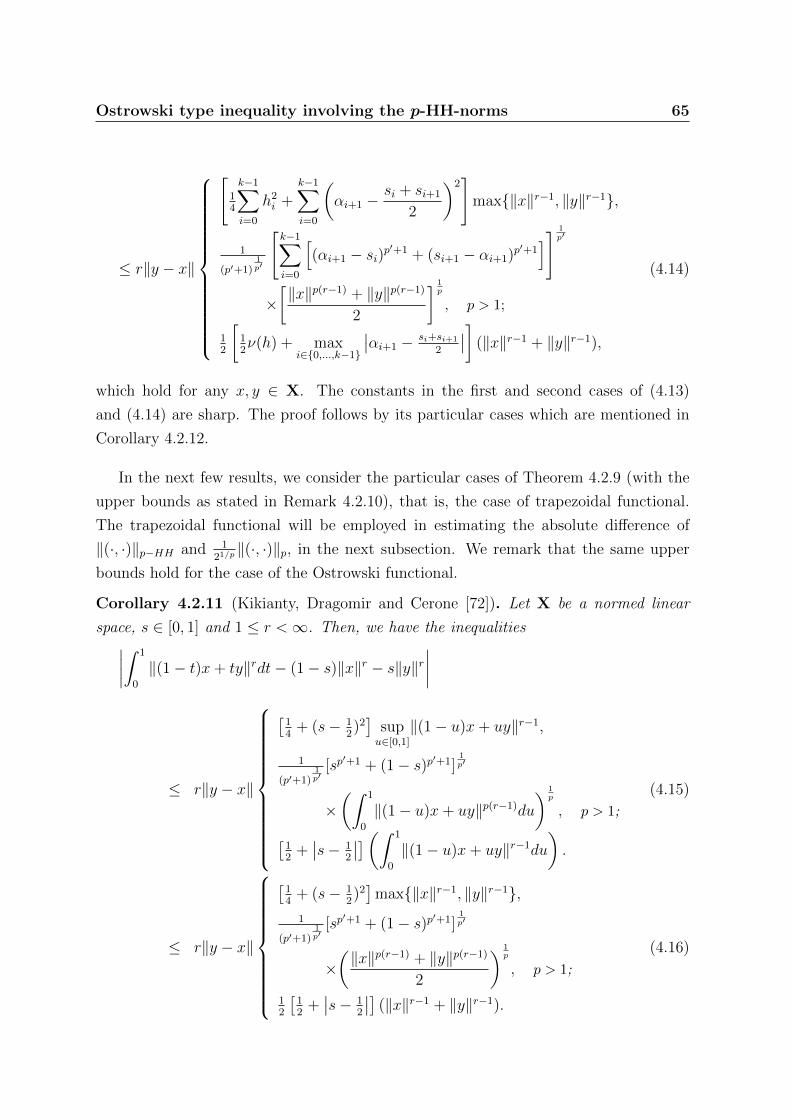
Ostrowski type inequality involving the p-HH-norms 65
≤ r‖y − x‖
[14
k−1∑i=0
h2i +
k−1∑i=0
(αi+1 −
si + si+1
2
)2]
max‖x‖r−1, ‖y‖r−1,
1
(p′+1)1p′
[k−1∑i=0
[(αi+1 − si)p
′+1 + (si+1 − αi+1)p′+1]] 1
p′
×[‖x‖p(r−1) + ‖y‖p(r−1)
2
] 1p
, p > 1;
12
[12ν(h) + max
i∈0,...,k−1
∣∣αi+1 − si+si+1
2
∣∣] (‖x‖r−1 + ‖y‖r−1),
(4.14)
which hold for any x, y ∈ X. The constants in the first and second cases of (4.13)
and (4.14) are sharp. The proof follows by its particular cases which are mentioned in
Corollary 4.2.12.
In the next few results, we consider the particular cases of Theorem 4.2.9 (with the
upper bounds as stated in Remark 4.2.10), that is, the case of trapezoidal functional.
The trapezoidal functional will be employed in estimating the absolute difference of
‖(·, ·)‖p−HH and 121/p‖(·, ·)‖p, in the next subsection. We remark that the same upper
bounds hold for the case of the Ostrowski functional.
Corollary 4.2.11 (Kikianty, Dragomir and Cerone [72]). Let X be a normed linear
space, s ∈ [0, 1] and 1 ≤ r <∞. Then, we have the inequalities∣∣∣∣∫ 1
0
‖(1− t)x+ ty‖rdt− (1− s)‖x‖r − s‖y‖r∣∣∣∣
≤ r‖y − x‖
[14
+ (s− 12)2]
supu∈[0,1]
‖(1− u)x+ uy‖r−1,
1
(p′+1)1p′
[sp′+1 + (1− s)p′+1]
1p′
×(∫ 1
0
‖(1− u)x+ uy‖p(r−1)du
) 1p
, p > 1;[12
+∣∣s− 1
2
∣∣](∫ 1
0
‖(1− u)x+ uy‖r−1du
).
(4.15)
≤ r‖y − x‖
[14
+ (s− 12)2]
max‖x‖r−1, ‖y‖r−1,1
(p′+1)1p′
[sp′+1 + (1− s)p′+1]
1p′
×(‖x‖p(r−1) + ‖y‖p(r−1)
2
) 1p
, p > 1;
12
[12
+∣∣s− 1
2
∣∣] (‖x‖r−1 + ‖y‖r−1).
(4.16)

66 Ostrowski type inequality involving the p-HH-norms
for any x, y ∈ X. The constants in the first and second cases of (4.15) and (4.16) are
sharp.
Proof. Choose s0 = 0, s1 = 1 and 0 = α0 < α1 = s < α2 = 1 in (4.13) and (4.14).
The sharpness of the constants follows by the particular case which is pointed out in
Corollary 4.2.12.
Corollary 4.2.12 (Kikianty, Dragomir and Cerone [72]). Particularly,∣∣∣∣∫ 1
0
‖(1− t)x+ ty‖2dt− (1− s)‖x‖2 − s‖y‖2
∣∣∣∣
≤ 2‖y − x‖
[14
+ (s− 12)2]
supu∈[0,1]
‖(1− u)x+ uy‖,
1
(p′+1)1p′
[sp′+1 + (1− s)p′+1]
1p′
×(∫ 1
0
‖(1− u)x+ uy‖pdu) 1
p
, p > 1;[12
+∣∣s− 1
2
∣∣](∫ 1
0
‖(1− u)x+ uy‖du),
(4.17)
≤ 2‖y − x‖
[14
+(s− 1
2
)2]
max‖x‖, ‖y‖,1
(p′+1)1p′
[sp′+1 + (1− s)p′+1
] 1p′
×(‖x‖p + ‖y‖p
2
) 1p
, p > 1;
12
[12
+∣∣s− 1
2
∣∣] (‖x‖+ ‖y‖),
(4.18)
for any x, y ∈ X. The constants in the first and second cases of (4.17) and (4.18) are
sharp.
We also have∣∣∣∣∫ 1
0
‖(1− t)x+ ty‖dt− (1− s)‖x‖ − s‖y‖∣∣∣∣ ≤
[1
4+
(s− 1
2
)2]‖y − x‖. (4.19)
The constant 14
in (4.19) is sharp.
Proof. We obtain (4.17) and (4.18) by choosing r = 2 in (4.15) and (4.16), respectively.
The proof for the sharpness of the constants is implied by Corollary 4.2.14. By choosing

Ostrowski type inequality involving the p-HH-norms 67
r = 1 in (4.15), we obtain∣∣∣∣∫ 1
0
‖(1− t)x+ ty‖dt− (1− s)‖x‖ − s‖y‖∣∣∣∣
≤ ‖y − x‖
14
+(s− 1
2
)2,
1
(p′+1)1p′
[sp′+1 + (1− s)p′+1
] 1p′ ,
12
+∣∣s− 1
2
∣∣ ,(4.20)
for any x, y ∈ X. Note that for all 1 < p′ <∞ and s ∈ [0, 1],
1. 14
+(s− 1
2
)2= s2+(1−s)2
2=
∫ 1
0
|t− s|dt,
2. 1
(p′+1)1p′
[sp′+1 + (1− s)p′+1
] 1p′ =
(∫ 1
0
|t− s|p′dt) 1
p′
,
3. 12
+∣∣s− 1
2
∣∣ = maxs, 1− s = supt∈[0,1]
|t− s|,
and ∫ 1
0
|t− s|dt ≤(∫ 1
0
|t− s|p′dt) 1
p′
≤ supt∈[0,1]
|t− s|
by the Holder inequality. Thus,
1
4+
(s− 1
2
)2
≤ 1
(p′ + 1)1p′
[sp′+1 + (1− s)p′+1]
1p′ (4.21)
≤ 1
2+
∣∣∣∣s− 1
2
∣∣∣∣ .We conclude that the constant 1
4+(s− 1
2
)2is best possible amongst the constants in
all cases of (4.20) and we obtain (4.19). The proof of the sharpness of the constant will
be given in Corollary 4.2.14.
4.2.2 Inequalities involving the p-HH-norm and the p-norm
In the next two results, we employ Corollaries 4.2.11 and 4.2.12 to estimate the absolute
difference of ‖(·, ·)‖p−HH and 121/p‖(·, ·)‖p.

68 Ostrowski type inequality involving the p-HH-norms
Corollary 4.2.13 (Kikianty, Dragomir and Cerone [72]). Let X be a normed linear
space and 1 ≤ r <∞. Then
0 ≤ ‖(x, y)‖rr2
− ‖(x, y)‖rr−HH
≤ r‖y − x‖
14‖(x, y)‖r−1
∞ ,
1
2(p′+1)1p′‖(x, y)‖r−1
p(r−1)−HH , p > 1;
12‖(x, y)‖r−1
(r−1)−HH ,
(4.22)
≤ r‖y − x‖
14‖(x, y)‖r−1
∞ ,
1
21p+1
(p′+1)1p′‖(x, y)‖r−1
p(r−1), p > 1;
14‖(x, y)‖r−1
r−1,
(4.23)
hold for any x, y ∈ X. The constants in the first and second cases of (4.22) and (4.23)
are sharp.
Proof. Choose s = 12
in (4.15) and (4.16). The sharpness of the constants follows by the
particular case which is pointed out in Corollary 4.2.14.
Corollary 4.2.14 (Kikianty, Dragomir and Cerone [72]). Particularly,
0 ≤ ‖(x, y)‖22
2− ‖(x, y)‖2
2−HH
≤ ‖y − x‖
12‖(x, y)‖∞,
1
(p′+1)1p′‖(x, y)‖p−HH , p > 1;
‖(x, y)‖1−HH ,
(4.24)
≤ ‖y − x‖
12‖(x, y)‖∞,
1
21p (p′+1)
1p′‖(x, y)‖p, p > 1;
12‖(x, y)‖1,
(4.25)
hold for any x, y ∈ X. The constants in the first and second cases of (4.24) and (4.25)
are sharp. We also have
0 ≤ ‖(x, y)‖1
2− ‖(x, y)‖1−HH ≤
1
4‖y − x‖. (4.26)
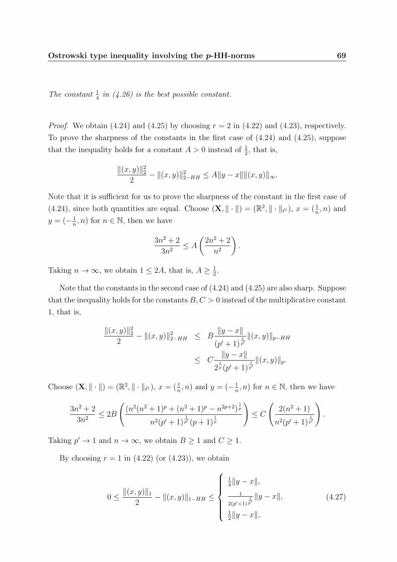
Ostrowski type inequality involving the p-HH-norms 69
The constant 14
in (4.26) is the best possible constant.
Proof. We obtain (4.24) and (4.25) by choosing r = 2 in (4.22) and (4.23), respectively.
To prove the sharpness of the constants in the first case of (4.24) and (4.25), suppose
that the inequality holds for a constant A > 0 instead of 12, that is,
‖(x, y)‖22
2− ‖(x, y)‖2
2−HH ≤ A‖y − x‖‖(x, y)‖∞.
Note that it is sufficient for us to prove the sharpness of the constant in the first case of
(4.24), since both quantities are equal. Choose (X, ‖ · ‖) = (R2, ‖ · ‖`1), x = ( 1n, n) and
y = (− 1n, n) for n ∈ N, then we have
3n2 + 2
3n2≤ A
(2n2 + 2
n2
).
Taking n→∞, we obtain 1 ≤ 2A, that is, A ≥ 12.
Note that the constants in the second case of (4.24) and (4.25) are also sharp. Suppose
that the inequality holds for the constants B,C > 0 instead of the multiplicative constant
1, that is,
‖(x, y)‖22
2− ‖(x, y)‖2
2−HH ≤ B‖y − x‖
(p′ + 1)1p′‖(x, y)‖p−HH
≤ C‖y − x‖
21p (p′ + 1)
1p′‖(x, y)‖p.
Choose (X, ‖ · ‖) = (R2, ‖ · ‖`1), x = ( 1n, n) and y = (− 1
n, n) for n ∈ N, then we have
3n2 + 2
3n2≤ 2B
((n2(n2 + 1)p + (n2 + 1)p − n2p+2)
1p
n2(p′ + 1)1p′ (p+ 1)
1p
)≤ C
(2(n2 + 1)
n2(p′ + 1)1p′
).
Taking p′ → 1 and n→∞, we obtain B ≥ 1 and C ≥ 1.
By choosing r = 1 in (4.22) (or (4.23)), we obtain
0 ≤ ‖(x, y)‖1
2− ‖(x, y)‖1−HH ≤
14‖y − x‖,
1
2(p′+1)1p′‖y − x‖,
12‖y − x‖,
(4.27)

70 Ostrowski type inequality involving the p-HH-norms
for any x, y ∈ X.
Note that for any 1 < p′ <∞, we have
1
4≤ 1
2(p′ + 1)1p′≤ 1
2
(the proof follows by choosing s = 12
in (4.21)). Therefore, 14
is the best possible among
the constants of all cases in (4.27) and we get (4.26). Now, suppose that the inequality
holds for any constant D > 0 instead of 14, that is,
‖(x, y)‖1
2− ‖(x, y)‖1−HH ≤ D‖y − x‖.
Choose (X, ‖ · ‖) = (R2, ‖ · ‖`1), x = (2, 1) and y = (2,−1) to obtain 12≤ 2D, that is,
D ≥ 14. Thus, the constant 1
4is sharp.
Remark 4.2.15 (The case of inner product space). If X is an inner product space, the
constant in the first case of (4.25) is not sharp, since
‖(x, y)‖22
2− ‖(x, y)‖2
2−HH =1
6‖y − x‖2,
and the fact that
1
6‖y − x‖2 ≤ 1
6‖y − x‖(‖x‖+ ‖y‖) ≤ 1
3‖y − x‖‖(x, y)‖∞.
The sharpness of the constant in the second case of (4.25) is not preserved in this
case, since we have the fact that
1
6‖y − x‖2 ≤ 1
6‖y − x‖(‖x‖+ ‖y‖) ≤ 1
3‖y − x‖‖(x, y)‖p,
and that 13≤ 1
21p (q+1)
1q.
The constant in the third case of (4.25) is not sharp, since
1
6‖y − x‖2 ≤ 1
6‖y − x‖‖(x, y)‖1.
The constant 14
in (4.26) remains sharp in this case. The proof follows by choosing
(X, ‖ · ‖) = (R, | · |), x = 1 and y = −1.

Ostrowski type inequality involving the p-HH-norms 71
4.3 Ostrowski inequality for convex functions on
linear spaces
A generalization of the classical Ostrowski inequality by considering the class of real
convex functions has been obtained in [35, 39]. The following result is a generalization
of an Ostrowski type inequality in [35] for convex functions defined on linear spaces.
Theorem 4.3.1 (Kikianty, Dragomir and Cerone [73]). Let X be a vector space, Ik : 0 =
s0 < s1 < · · · < sk−1 < sk = 1 be a partition of the interval [0, 1], αi (i = 0, . . . , k + 1)
be k + 2 points such that α0 = 0, αi ∈ [si−1, si], (i = 1, . . . , k) and αk+1 = 1. If
f : [x, y] ⊂ X→ R is a convex function on the segment [x, y], then we have
1
2
k−1∑i=0
(si+1 − αi+1)2
(∇+f [(1− αi+1)x+ αi+1y]
)(y − x)
−(αi+1 − si)2(∇−f [(1− αi+1)x+ αi+1y]
)(y − x)
≤
k∑i=0
(αi+1 − αi)f [(1− si)x+ siy]−∫ 1
0
f [(1− t)x+ ty]dt (4.28)
≤ 1
2
k−1∑i=0
(si+1 − αi+1)2
(∇−f [(1− si+1)x+ si+1y]
)(y − x)
−(αi+1 − si)2(∇+f [(1− si)x+ siy]
)(y − x)
.
The constant 12
is sharp in both inequalities.
Proof. Consider the function g(t) = f [(1− t)x+ ty] defined on [0, 1]. Since f is a convex
function on [x, y], g is also convex on [0, 1]. Therefore, we may apply Lemma 4.1.4. The
right-sided and left-sided derivatives of g can be computed as follows:
g′±(t) =(∇±f [(1− t)x+ ty]
)(y − x), t ∈ [0, 1].
We obtained the desired result by employing (4.3) of Lemma 4.1.4 for g. The sharpness of
the constants follows by some particular cases which will be considered later in Corollary
4.3.6.
The following result is a particular case of Theorem 4.3.1 for a trapezoidal type
functional.

72 Ostrowski type inequality involving the p-HH-norms
Corollary 4.3.2 (Kikianty, Dragomir and Cerone [73]). Let X be a vector space, x, y ∈X, x 6= y and f : [x, y] ⊂ X → R be a convex function on the segment [x, y]. Then for
any s ∈ (0, 1) one has the inequality
1
2[(1− s)2
(∇+f [(1− s)x+ sy]
)(y − x)− s2
(∇−f [(1− s)x+ sy]
)(y − x)]
≤ sf(x) + (1− s)f(y)−∫ 1
0
f [(1− t)x+ ty]dt (4.29)
≤ 1
2[(1− s)2(∇−f(y))(y − x)− s2(∇+f(x))(y − x)].
The constant 12
is sharp in both inequalities.
Proof. The result can be obtained by choosing k = 1 and s0 = α0 = 0, α1 = s ∈ (0, 1)
and s1 = α2 = 1 in Theorem 4.3.1. The sharpness of the constants will be proven later
in Corollary 4.3.6.
An alternative proof of Corollary 4.3.2 can be found in Theorem 2.4 of Dragomir
[34]. The following result provides an improvement for the second Hermite-Hadamard
inequality [34].
Remark 4.3.3. By letting s = 12
in (4.29) we have
1
8
[(∇+f
(x+ y
2
))(y − x)−
(∇−f
(x+ y
2
))(y − x)
]≤ f(x) + f(y)
2−∫ 1
0
f [(1− t)x+ ty]dt (4.30)
≤ 1
8[(∇−f(y))(y − x)− (∇+f(x))(y − x)].
The constant 18
is sharp, which proof can be found in Corollary 4.3.6.
4.3.1 Application for semi-inner products
Let (X, ‖ · ‖) be a normed linear space. We obtain the following inequalities for the
semi-inner products 〈·, ·〉s and 〈·, ·〉i.
Corollary 4.3.4 (Kikianty, Dragomir and Cerone [73]). Let Ik : 0 = s0 < s1 < · · · <sk−1 < sk = 1 be a partition of the interval [0, 1] and αi (i = 0, . . . , k+ 1) be k+ 2 points
such that α0 = 0, αi ∈ [si−1, si], (i = 1, . . . , k) and αk+1 = 1. Assume that 1 ≤ p < ∞.

Ostrowski type inequality involving the p-HH-norms 73
Then,
1
2p
k−1∑i=0
‖(1− αi+1)x+ αi+1y‖p−2[(si+1 − αi+1)2〈y − x, (1− αi+1)x+ αi+1y〉s
−(αi+1 − si)2〈y − x, (1− αi+1)x+ αi+1y〉i]
≤k∑i=0
(αi+1 − αi)‖(1− si)x+ siy‖p −∫ 1
0
‖(1− t)x+ ty‖pdt (4.31)
≤ 1
2pk−1∑i=0
[(si+1 − αi+1)2‖(1− si+1)x+ si+1y‖p−2〈y − x, (1− si+1)x+ si+1y〉i
−(αi+1 − si)2‖(1− si)x+ siy‖p−2〈y − x, (1− si)x+ siy〉s],
holds for any x, y ∈ X whenever p ≥ 2; otherwise, it holds for linearly independent
x, y ∈ X.
The constant 12
is sharp in both inequalities.
Proof. Apply Theorem 4.3.1 to the convex function fp(x) = ‖x‖p, where x ∈ X and
1 ≤ p < ∞. Note the use of identity (4.4) of Example 4.2.2. The sharpness of the
constants will be proven later in Corollary 4.3.6.
The following result is a particular case of Corollary 4.3.4 for a trapezoidal type
functional.
Corollary 4.3.5 (Kikianty, Dragomir and Cerone [73]). Let x and y be any two vectors
in X, σ ∈ (0, 1) and 1 ≤ p <∞. Then
1
2p‖(1− σ)x+ σy‖p−2[(1− σ)2〈y − x, (1− σ)x+ σy〉s
−σ2〈y − x, (1− σ)x+ σy〉i]
≤ σ‖x‖p + (1− σ)‖y‖p −∫ 1
0
‖(1− t)x+ ty‖pdt (4.32)
≤ 1
2p[(1− σ)2‖y‖p−2〈y − x, y〉i − σ2‖x‖p−2〈y − x, x〉s],
holds for any x, y ∈ X whenever p ≥ 2; otherwise, it holds for linearly independent
x, y ∈ X.
The constant 12
is sharp in both inequalities.

74 Ostrowski type inequality involving the p-HH-norms
We also have two particular cases that are of interest, namely
(1− σ)2〈y − x, (1− σ)x+ σy〉s − σ2〈y − x, (1− σ)x+ σy〉i
≤ σ‖x‖2 + (1− σ)‖y‖2 −∫ 1
0
‖(1− t)x+ ty‖2dt (4.33)
≤ (1− σ)2〈y − x, y〉i − σ2〈y − x, x〉s,
for any x, y ∈ X and
1
2
[(1− σ)2
⟨y − x, (1− σ)x+ σy
‖(1− σ)x+ σy‖
⟩s
− σ2
⟨y − x, (1− σ)x+ σy
‖(1− σ)x+ σy‖
⟩i
]≤ σ‖x‖+ (1− σ)‖y‖ −
∫ 1
0
‖(1− t)x+ ty‖dt (4.34)
≤ 1
2
[(1− σ)2
⟨y − x, y
‖y‖
⟩i
− σ2
⟨y − x, x
‖x‖
⟩s
],
for any linearly independent x, y ∈ X. The constants in (4.33) and (4.34) are sharp.
Proof. Choose k = 1, s0 = α0 = 0, α1 = σ ∈ (0, 1) and s1 = α2 = 1 in Proposition 4.3.4.
As an alternative proof, this result can be obtained by choosing f(x) = ‖x‖p, (1 ≤ p <
∞) and s = σ in Corollary 4.3.2 (note the use of identity (4.4) of Example 4.2.2). Take
p = 2 and p = 1 in (4.32) to obtain (4.33) and (4.34). The sharpness of the constants
will be proven later in Corollary 4.3.6 by considering some particular cases.
We note that (4.33) and (4.34) recapture the results of Dragomir [34, Proposition
3.1 and Proposition 3.2]. However, the sharpness of the constants was not considered in
the paper.
4.3.2 Inequalities involving the p-HH-norm and the p-norm
The main result of this section follows from Section 4.3.1. Furthermore, it provides an
improvement for the Hermite-Hadamard inequalities (1.11).
The next corollary gives a generalization of the results by Dragomir [34]. We also
state some particular cases which recapture the results by Dragomir [34]. However, the
sharpness of the constants in these inequalities were not considered. Here, we provide
the proof for the sharpness of these inequalities.

Ostrowski type inequality involving the p-HH-norms 75
Corollary 4.3.6 (Kikianty, Dragomir and Cerone [73]). Let (X, ‖·‖) be a normed linear
space and 1 ≤ p <∞. Then,
0 ≤ 1
8p
∥∥∥∥y + x
2
∥∥∥∥p−2 [⟨y − x, y + x
2
⟩s
−⟨y − x, y + x
2
⟩i
]≤‖(x, y)‖pp
2− ‖(x, y)‖pp−HH (4.35)
≤ 1
8p[‖y‖p−2〈y − x, y〉i − ‖x‖p−2〈y − x, x〉s],
holds for any x, y ∈ X whenever p ≥ 2; otherwise, it holds for linearly independent
x, y ∈ X.
In particular, we have
0 ≤ 1
8[〈y − x, y + x〉s − 〈y − x, y + x〉i]
≤ ‖(x, y)‖22
2− ‖(x, y)‖2
2−HH (4.36)
≤ 1
4[〈y − x, y〉i − 〈y − x, x〉s],
for any x, y ∈ X and
0 ≤ 1
8
[⟨y − x,
y+x2
‖y+x2‖
⟩s
−⟨y − x,
y+x2
‖y+x2‖
⟩i
]
≤ ‖(x, y)‖1
2− ‖(x, y)‖1−HH (4.37)
≤ 1
8
[⟨y − x, y
‖y‖
⟩i
−⟨y − x, x
‖x‖
⟩s
],
for any linearly independent x, y ∈ X.
The constants in (4.35), (4.36) and (4.37) are sharp.
Proof. We obtain (4.35) by taking σ = 12
in (4.32). We may also obtain (4.35) by taking
f(x) = ‖x‖p (1 ≤ p < ∞) in Remark 4.3.3. We get (4.36) and (4.37) by taking p = 2
and p = 1, respectively, in (4.35).
Note that we may also obtain (4.36) from (4.33) of Corollary 4.3.5 and (4.37) from
(4.34) of Corollary 4.3.5, by letting σ = 12. The sharpness of the constants in (4.35)
follows by the sharpness of the constants in (4.36) and (4.37) as its particular cases.
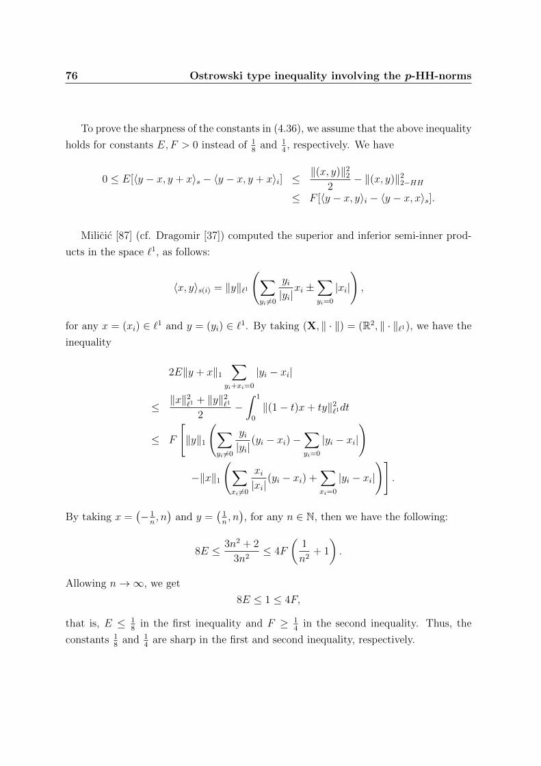
76 Ostrowski type inequality involving the p-HH-norms
To prove the sharpness of the constants in (4.36), we assume that the above inequality
holds for constants E,F > 0 instead of 18
and 14, respectively. We have
0 ≤ E[〈y − x, y + x〉s − 〈y − x, y + x〉i] ≤‖(x, y)‖2
2
2− ‖(x, y)‖2
2−HH
≤ F [〈y − x, y〉i − 〈y − x, x〉s].
Milicic [87] (cf. Dragomir [37]) computed the superior and inferior semi-inner prod-
ucts in the space `1, as follows:
〈x, y〉s(i) = ‖y‖`1(∑yi 6=0
yi|yi|
xi ±∑yi=0
|xi|
),
for any x = (xi) ∈ `1 and y = (yi) ∈ `1. By taking (X, ‖ · ‖) = (R2, ‖ · ‖`1), we have the
inequality
2E‖y + x‖1
∑yi+xi=0
|yi − xi|
≤‖x‖2
`1 + ‖y‖2`1
2−∫ 1
0
‖(1− t)x+ ty‖2`1dt
≤ F
[‖y‖1
(∑yi 6=0
yi|yi|
(yi − xi)−∑yi=0
|yi − xi|
)
−‖x‖1
(∑xi 6=0
xi|xi|
(yi − xi) +∑xi=0
|yi − xi|
)].
By taking x =(− 1n, n)
and y =(
1n, n), for any n ∈ N, then we have the following:
8E ≤ 3n2 + 2
3n2≤ 4F
(1
n2+ 1
).
Allowing n→∞, we get
8E ≤ 1 ≤ 4F,
that is, E ≤ 18
in the first inequality and F ≥ 14
in the second inequality. Thus, the
constants 18
and 14
are sharp in the first and second inequality, respectively.

Ostrowski type inequality involving the p-HH-norms 77
To prove the sharpness of the constants in (4.37), we assume that the above inequality
holds for constants G,H > 0 instead of 18, that is
0 ≤ G
[⟨y − x,
y+x2
‖y+x2‖
⟩s
−⟨y − x,
y+x2
‖y+x2‖
⟩i
]
≤ ‖(x, y)‖1
2− ‖(x, y)‖1−HH
≤ H
[⟨y − x, y
‖y‖
⟩i
−⟨y − x, x
‖x‖
⟩s
].
Again, we choose (X, ‖ · ‖) = (R2, ‖ · ‖`1). Therefore we have the following inequalities
0 ≤ 2G∑
yi+xi=0
|yi − xi|
≤ ‖x‖`1 + ‖y‖`12
−∫ 1
0
‖(1− t)x+ ty‖`1dt
≤ H
[∑yi 6=0
yi|yi|
(yi − xi)−∑yi=0
|yi − xi| −∑xi 6=0
xi|xi|
(yi − xi)−∑xi=0
|yi − xi|
],
for any linearly independent x and y. Let x = (1, 0) and y = (−1, 1). Clearly x and
y are linearly independent. Therefore the above inequality holds for these vectors. We
have
4G ≤ 1
2≤ 4H,
that is, G ≤ 18
in the first inequality and H ≥ 18
in the second inequality. Thus, the
constant 18
is sharp in both inequalities.
Remark 4.3.7 (The case of inner product spaces). Let X be an inner product space,
with the inner product 〈·, ·〉. Then, by Corollary 4.3.6, we have
0 ≤‖(x, y)‖pp
2− ‖(x, y)‖pp−HH
≤ 1
8p〈y − x, y‖y‖p−2 − x‖x‖p−2〉, (4.38)
holds for any x, y ∈ X whenever p ≥ 2; otherwise, it holds for nonzero x, y ∈ X.
Particularly, for p = 2, we have
0 ≤ ‖(x, y)‖22
2− ‖(x, y)‖2
2−HH ≤1
4[〈y − x, y − x〉] =
1
4‖y − x‖2,

78 Ostrowski type inequality involving the p-HH-norms
for any x, y ∈ X. The constant 14
is not the best possible constant in this case, since we
always have‖(x, y)‖2
2
2− ‖(x, y)‖2
2−HH =1
6‖y − x‖2.
If p = 1, then
0 ≤ ‖(x, y)‖1
2− ‖(x, y)‖1−HH ≤
1
8
⟨y − x, y
‖y‖− x
‖x‖
⟩,
for any nonzero x, y ∈ X. We obtain a nontrivial equality by choosing X = R and
multiplication as its inner product (which induces the absolute value for its norm),
x = 1 and y = −1. Thus, the constant 18
is sharp.
Conjecture 4.3.8. We conjecture that the constant 18
in (4.38) is not sharp for any
p > 1. Utilizing MAPLE for the real-valued functions
Fp(x, y) :=|x|p + |y|p
2−∫ 1
0
|(1− t)x+ ty|pdt,
Gp(x, y) :=1
8p(y − x)(y|y|p−2 − x|x|p−2),
for (x, y) ∈ R2, we observe that for several values of p > 1, the equation Fp(x, y) =
Gp(x, y) = k 6= 0 has no solution in R2. Again, we utilize MAPLE to plot these
functions with the choice of p = 3, as may be seen in Figure 4.1. One may see that the
two surfaces in Figure 4.1 intersect on the level set k = 0. Therefore, the constant 18
is
not sharp for these values of p, since we have no nontrivial equality. However, we do not
have an analytical proof for this claim.
000
0.5
1
0.5 0.5
1.5
2
1 1
2.5
3
x y
1.5 1.52 2
Figure 4.1: Plot of F3 and G3

Ostrowski type inequality involving the p-HH-norms 79
4.4 Comparison analysis
We want to compare the two bounds that have been obtained in Sections 4.2 and 4.3,
that is,
1
8r(〈y − x, y‖y‖r−2〉i − 〈y − x, x‖x‖r−2〉s) and
1
4r‖y − x‖max‖x‖r−1, ‖y‖r−1.
The bound that is obtained in Section 4.2 is simpler in the sense that it only involves
the given norm, while the bound in Section 4.3 involves not only the given norm, but
also the superior and inferior semi-inner products associated with the norm. However,
the bound in Section 4.3 is proven to be better than that of Section 4.2, when X is an
inner product space for r = 1 and r = 2. The verification is presented in the following.
Let (X, 〈·, ·〉) be an inner product space.
Case of r = 1. We wish to compare
1
8
⟨y − x, y
‖y‖− x
‖x‖
⟩and
1
4‖y − x‖,
for nonzero x, y ∈ X. To do so, we employ the Dunkl-Williams inequality [49, p. 53]
(cf. Kirk and Smiley [76, p. 890] and Mercer [86, p. 448])∥∥∥∥ x
‖x‖− y
‖y‖
∥∥∥∥ ≤ 2‖x− y‖‖x‖+ ‖y‖
, (4.39)
which holds for nonzero x and y in an inner product space X. Now, for x, y ∈ X where
x, y 6= 0, we have
1
8
⟨y − x, y
‖y‖− x
‖x‖
⟩≤ 1
8‖y − x‖
∥∥∥∥ y
‖y‖− x
‖x‖
∥∥∥∥≤ 1
4‖y − x‖ ‖x− y‖
‖x‖+ ‖y‖
≤ 1
4‖y − x‖‖x‖+ ‖y‖
‖x‖+ ‖y‖=
1
4‖y − x‖.
We conclude that the bound in Section 4.3 is sharper.
Case of r = 2. We want to compare
1
4〈y − x, y − x〉 =
1
4‖y − x‖2 and
1
2‖y − x‖max‖x‖, ‖y‖.

80 Ostrowski type inequality involving the p-HH-norms
For all x, y ∈ X, we have
1
4‖y − x‖2 ≤ 1
4‖y − x‖(‖x‖+ ‖y‖) ≤ 1
2‖y − x‖max‖x‖, ‖y‖.
We conclude that the bound in Section 4.3 is sharper.
Case of 1 < r <∞, r 6= 2. We conjecture that:
Conjecture 4.4.1. In an inner product space (X, 〈·, ·〉), the following inequality
1
8r〈y − x, y‖y‖r−2 − x‖x‖r−2〉 ≤ 1
4r‖y − x‖max‖x‖r−1, ‖y‖r−1
holds for any x, y ∈ X whenever r ≥ 2; otherwise it holds for any nonzero x, y ∈ X.
We observe that the above statement is true in some cases. Taking X = R and
multiplication as its inner product and utilizing MAPLE for the following functions
Φ(x, y) :=1
4r|y − x|max|x|r−1, |y|r−1 − 1
8r(y − x)(y|y|r−2 − x|x|r−2),
for x, y ∈ R, we observe that for several values of r, we have Φ(x, y) ≥ 0 for any x, y ∈ X.
Figure 4.2 gives us the plot of Φ with the choice of r = 3. However, we have no analytical
proof for this statement.
-1
-1-0.5
-0.5000
x
y
0.1
0.50.5
0.2
1
0.3
1
0.4
Figure 4.2: Plot of Φ for r = 3.

Ostrowski type inequality involving the p-HH-norms 81
Conjecture 4.4.2. In a normed linear space (X, ‖ · ‖), the following inequality
1
8r(〈y − x, y‖y‖r−2〉i − 〈y − x, x‖x‖r−2〉s) ≤
1
4r‖y − x‖max‖x‖r−1, ‖y‖r−1
holds for any x, y ∈ X whenever r ≥ 2; otherwise it holds for any nonzero x, y ∈ X (here,
〈·, ·〉s(i) is the superior (inferior) semi-inner product with respect to the norm ‖ · ‖).
We observe that the above statement is true in some cases. In (X, ‖·‖) = (R2, ‖·‖`1),consider the case of r = 1, we have the following functions
f(x, y) =1
8
[∑yi 6=0
yi|yi|
(yi − xi)−∑yi=0
|yi − xi| −∑xi 6=0
xi|xi|
(yi − xi)−∑xi=0
|yi − xi|
],
and
g(x, y) =1
4‖y − x‖1,
for x, y ∈ R2. We observe that f(x, y) ≤ g(x, y) for some x, y ∈ R2. We choose x = (1, 0)
and y = (a, b) (a, b 6= 0) and plot the nonnegative function Ψ(a, b) := g(x, y)− f(x, y) =14(|a− 1|+ |b|)− 1
8
(a(a−1)|a| + b2
|b| − (a− 1)− |b|)
in Figure 4.3. However, we do not have
an analytical proof for this statement.
-4
-4-2
-20
00
b
2
0.5
a 2
4
1
4
1.5
2
Figure 4.3: Plot of Ψ

82

Chapter 5
Gruss type inequality involving the
p-HH-norms
In Chapter 4, we provide some inequalities of Ostrowski type, which involve the p-HH-
norms and the p-norms. In the same spirit, we continue the work in this chapter, in
considering some bounds to estimate the difference of ‖(·, ·)‖p+qp+q−HH and the product
‖(·, ·)‖pp−HH‖(·, ·)‖qq−HH for any p, q ≥ 1. This difference, however, is a particular type
of Cebysev functional. The results in this chapter are mainly taken from the author’s
research paper with Dragomir and Cerone [74].
In Section 5.1, we recall some known results regarding the Cebysev functional. These
results are then applied to obtain upper bounds in estimating the Cebysev difference of
‖(x, y)‖p+qp+q−HH and ‖(x, y)‖pp−HH‖(x, y)‖qq−HH (p, q ≥ 1), in Section 5.2. Some of these
inequalities are proven to be sharp.
In Section 5.3, we establish some sharp bounds for the generalized Cebysev functional
in order to approximate the Riemann-Stieltjes integral for differentiable convex integrand
and monotonically increasing integrator. The result follows by utilizing an Ostrowski
type inequality.
We apply this result in Section 5.4, for the Cebysev functional; and the obtained
bounds are sharp. A similar result is established for a general convex function with the
obtained bounds are shown to be also sharp. By applying the result for the p-HH-norms,
we also procure some upper and lower bounds for the difference of ‖(x, y)‖p+qp+q−HH and
‖(x, y)‖pp−HH‖(x, y)‖qq−HH (p, q ≥ 1). These bounds are proven to be sharp.
83

84 Gruss type inequality involving the p-HH-norms
5.1 Gruss inequality and Cebysev functional
We start by considering the following definition.
Definition 5.1.1 (Hardy, Littlewood and Polya [58]). Let f and g be two real-valued
functions defined on an interval I. We say that f and g are similarly ordered, if and
only if
[f(t)− f(s)][g(t)− g(s)] ≥ 0
for any t, s ∈ I; and oppositely ordered if the inequality is always reversed.
Let f, g : [a, b] → R be two Lebesgue integrable functions. If f and g are similarly
ordered, then ∫ b
a
f(t)g(t)dt ≥ 1
b− a
∫ b
a
f(t)dt
∫ b
a
g(t)dt. (5.1)
The inequality is reversed when f and g are oppositely ordered. Equality occurs when f
and g are constants. Inequality (5.1) is known in the literature as the Cebysev inequality
[91, p. 239].
For two Lebesgue integrable functions f, g : [a, b] → R, consider the Cebysev func-
tional (the Cebysev difference)
T (f, g) :=1
b− a
∫ b
a
f(t)g(t)dt− 1
b− a
∫ b
a
f(t)dt · 1
b− a
∫ b
a
g(t)dt.
In 1935, Gruss proved the following inequality which bounds the Cebysev functional [91,
p. 295–296]:
|T (f, g)| ≤ 1
4(Φ− φ)(Γ− γ), (5.2)
provided that f and g satisfy the conditions
φ ≤ f(t) ≤ Φ and γ ≤ g(t) ≤ Γ for all t ∈ [a, b].
The constant 14
is best possible and is achieved for
f(t) = g(t) = sgn
(t− a+ b
2
).

Gruss type inequality involving the p-HH-norms 85
Some related results regarding the sharp upper bounds for this functional can be sum-
marized as follows:
1. Cebysev (1882): If f, g are continuously differentiable functions on [a, b], then
|T (f, g)| ≤ 1
12‖f ′‖L∞‖g′‖L∞(b− a)2. (5.3)
Equality holds if and only if f ′ and g′ are constants [91, p. 297]. It is also valid for
absolutely continuous functions f, g where f ′, g′ ∈ L∞[a, b].
2. Ostrowski (1970): Suppose that f is Lebesgue integrable on [a, b] and m,M ∈ Rsuch that −∞ ≤ m ≤ f ≤M ≤ ∞. If g is absolutely continuous and g′ ∈ L∞[a, b],
then
|T (f, g)| ≤ 1
8(b− a)(M −m)‖g′‖L∞ , (5.4)
and the constant 18
is the best possible [91, p. 300].
3. Lupas (1973): If f, g are absolutely continuous, f ′, g′ ∈ L2[a, b], then
|T (f, g)| ≤ 1
π2(b− a)‖f ′‖L2‖g′‖L2 . (5.5)
Equality valid if and only if
f(x) = A+B sin
[π
b− a
(x− a+ b
2
)]and
g(x) = C +D sin
[π
b− a
(x− a+ b
2
)],
where A, B, C and D are constants [91, p. 301].
These results are applied in Section 5.2 to obtain upper bounds in estimating the Cebysev
difference ‖(x, y)‖p+qp+q−HH and ‖(x, y)‖pp−HH‖(x, y)‖qq−HH , where p, q ≥ 1 and (x, y) in
the Cartesian space X2 of the normed space X. We refer to the work by Dragomir and
Fedotov [40] for more results regarding the Cebysev functional.
In order to approximate the Riemann-Stieltjes integral, the generalized Cebysev func-
tional
D(f, u) :=
∫ b
a
f(t)du(t)− 1
b− a[u(b)− u(a)]
∫ b
a
f(s)ds

86 Gruss type inequality involving the p-HH-norms
is employed, where f is Riemann integrable and Stieltjes integrable with respect to a
function u. Some bounds for D, when u is monotonically non-decreasing, were obtained
by Dragomir in 2004 [36]. The results are summarized as follows:
1. If f : [a, b]→ R is L-Lipschitzian on [a, b], then
|D(f, u; a, b)| ≤ 1
2L(b− a)[u(b)− u(a)−K(u; a, b)]
≤ 1
2L(b− a)[u(b)− u(a)],
where
K(u; a, b) :=4
(b− a)2
∫ b
a
u(t)
(t− a+ b
2
)dt ≥ 0.
The constant 12
is best possible in both inequalities.
2. If f : [a, b]→ R is a function of bounded variation on [a, b] and∫ baf(t)du(t) exists,
then
|D(f, u; a, b)| ≤ [u(b)− u(a)−Q(u; a, b)]b∨a
(f)
≤ [u(b)− u(a)]b∨a
(f),
where∨ba(f) is the total variation of f on [a, b] and
Q(u; a, b) :=1
b− a
∫ b
a
sgn
(t− a+ b
2
)dt ≥ 0.
The first inequality is sharp.
In Section 5.3, we establish some sharp bounds for D for the case of differentiable convex
integrand and monotonically increasing integrator. Furthermore, the results is employed
to bound the Cebysev difference ‖(x, y)‖p+qp+q−HH − ‖(x, y)‖pp−HH‖(x, y)‖qq−HH .
5.2 Inequalities involving the p-HH-norms
In this section, we obtain some norm inequalities involving the p-HH-norms. The fol-
lowing lemma is a norm inequality of Cebysev type.
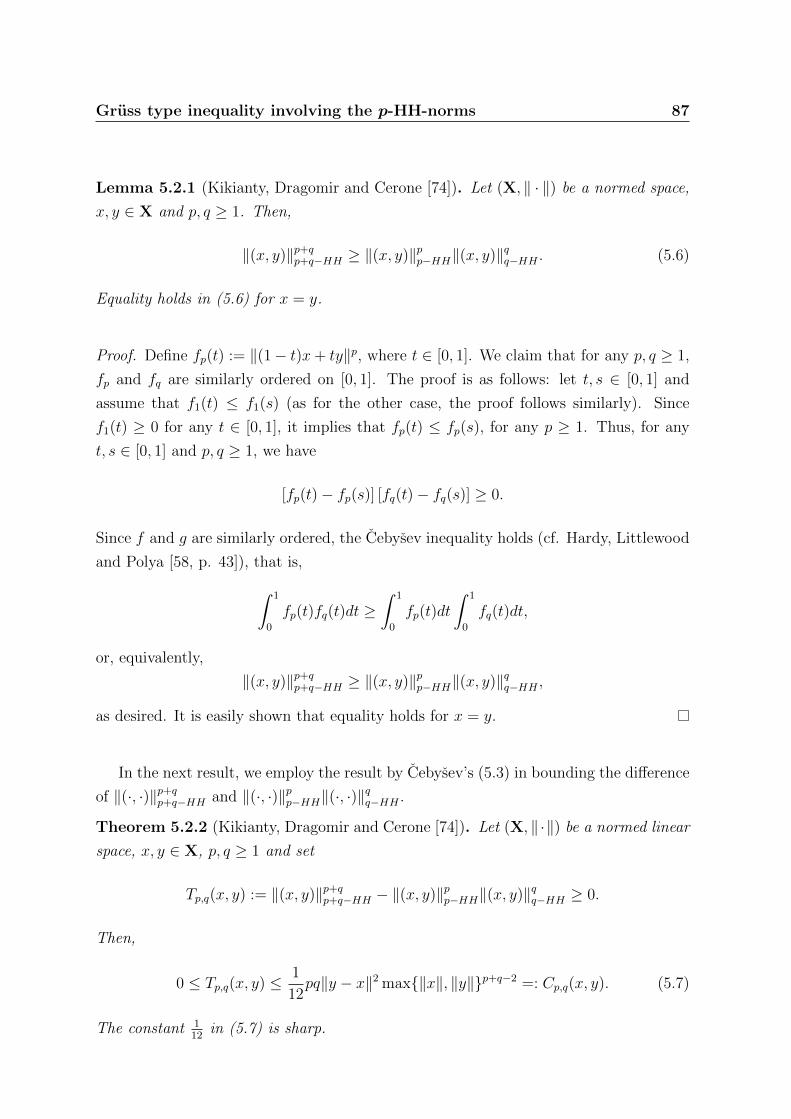
Gruss type inequality involving the p-HH-norms 87
Lemma 5.2.1 (Kikianty, Dragomir and Cerone [74]). Let (X, ‖ · ‖) be a normed space,
x, y ∈ X and p, q ≥ 1. Then,
‖(x, y)‖p+qp+q−HH ≥ ‖(x, y)‖pp−HH‖(x, y)‖qq−HH . (5.6)
Equality holds in (5.6) for x = y.
Proof. Define fp(t) := ‖(1− t)x+ ty‖p, where t ∈ [0, 1]. We claim that for any p, q ≥ 1,
fp and fq are similarly ordered on [0, 1]. The proof is as follows: let t, s ∈ [0, 1] and
assume that f1(t) ≤ f1(s) (as for the other case, the proof follows similarly). Since
f1(t) ≥ 0 for any t ∈ [0, 1], it implies that fp(t) ≤ fp(s), for any p ≥ 1. Thus, for any
t, s ∈ [0, 1] and p, q ≥ 1, we have
[fp(t)− fp(s)] [fq(t)− fq(s)] ≥ 0.
Since f and g are similarly ordered, the Cebysev inequality holds (cf. Hardy, Littlewood
and Polya [58, p. 43]), that is,∫ 1
0
fp(t)fq(t)dt ≥∫ 1
0
fp(t)dt
∫ 1
0
fq(t)dt,
or, equivalently,
‖(x, y)‖p+qp+q−HH ≥ ‖(x, y)‖pp−HH‖(x, y)‖qq−HH ,
as desired. It is easily shown that equality holds for x = y.
In the next result, we employ the result by Cebysev’s (5.3) in bounding the difference
of ‖(·, ·)‖p+qp+q−HH and ‖(·, ·)‖pp−HH‖(·, ·)‖qq−HH .
Theorem 5.2.2 (Kikianty, Dragomir and Cerone [74]). Let (X, ‖·‖) be a normed linear
space, x, y ∈ X, p, q ≥ 1 and set
Tp,q(x, y) := ‖(x, y)‖p+qp+q−HH − ‖(x, y)‖pp−HH‖(x, y)‖qq−HH ≥ 0.
Then,
0 ≤ Tp,q(x, y) ≤ 1
12pq‖y − x‖2 max‖x‖, ‖y‖p+q−2 =: Cp,q(x, y). (5.7)
The constant 112
in (5.7) is sharp.

88 Gruss type inequality involving the p-HH-norms
Proof. Let x, y ∈ X and define
f(t) = ‖(1− t)x+ ty‖p and g(t) = ‖(1− t)x+ ty‖q,
for t ∈ [0, 1]. Since both f and g are convex, they are absolutely continuous; also f ′ and
g′ exist almost everywhere on [0, 1]. Therefore,
f ′(t) =(∇±‖ · ‖p[(1− t)x+ ty]
)(y − x)
= p‖(1− t)x+ ty‖p−2〈y − x, (1− t)x+ ty〉s(i),
where 〈·, ·〉s(i) is the superior (inferior) semi-inner product (cf. identity (4.4) of Example
4.2.2) and by the Cauchy-Schwarz inequality, we get
‖f ′‖L∞ = supt∈[0,1]
p‖(1− t)x+ ty‖p−2|〈y − x, (1− t)x+ ty〉s(i)|
≤ p‖y − x‖ supt∈[0,1]
‖(1− t)x+ ty‖p−1
= p‖y − x‖max‖x‖, ‖y‖p−1.
Similarly for g, we have ‖g′‖L∞ ≤ q‖y − x‖max‖x‖, ‖y‖q−1. Due to Cebysev’s result
(5.3), we thus conclude
Tp,q(x, y) ≤ 1
12‖f ′‖L∞‖g′‖L∞
≤ 1
12pq‖y − x‖2 max‖x‖, ‖y‖p+q−2.
To prove the sharpness of the constant, we assume that inequality (5.7) holds for a
constant A > 0 instead of 112
, that is,
‖(x, y)‖p+qp+q−HH − ‖(x, y)‖pp−HH‖(x, y)‖qq−HH≤ A pq‖y − x‖2 max‖x‖, ‖y‖p+q−2.
Choose p = 1, q = 1, X = R and 0 < x < y, to obtain
1
3
(x2 + xy + y2
)−(y + x
2
)2
=1
12(y − x)2 ≤ A(y − x)2.
Since x 6= y, A ≥ 112
which completes the proof.

Gruss type inequality involving the p-HH-norms 89
Similarly to Theorem 5.2.2, we employ the results by Gruss, Ostrowski and Lupas
to obtain more norm inequalities. We start by setting the following quantities for x, y ∈(X, ‖ · ‖) and p, q ≥ 1:
Gp,q(x, y) :=1
4max‖x‖, ‖y‖p+q
Op,q(x, y) :=1
8q‖y − x‖max‖x‖, ‖y‖p+q−1, and
Lp,q(x, y) :=1
π2pq‖y − x‖2‖(x, y)‖p−1
(2p−2)−HH‖(x, y)‖q−1(2q−2)−HH .
The following proposition is due to the results by Gruss, Ostrowski and Lupas. However,
the sharpness of these inequalities are yet to be proven.
Proposition 5.2.3 (Kikianty, Dragomir and Cerone [74]). Under the assumptions of
Theorem 5.2.2 and the above notation, we have
0 ≤ Tp,q(x, y) ≤ Gp,q(x, y),
0 ≤ Tp,q(x, y) ≤ Op,q(x, y), and
0 ≤ Tp,q(x, y) ≤ Lp,q(x, y),
for any p, q ≥ 1 and x, y ∈ X.
Proof. Let x, y ∈ X and define f(t) = ‖(1− t)x + ty‖p and g(t) = ‖(1− t)x + ty‖q, for
t ∈ [0, 1]. Since p, q ≥ 1, we have
0 ≤ f(t) ≤ max‖x‖, ‖y‖p and 0 ≤ g(t) ≤ max‖x‖, ‖y‖q.
Then, due to the result by Gruss (5.2), we have
Tp,q(x, y) ≤ 1
4max‖x‖, ‖y‖p+q = Gp,q(x, y).
Since g is absolutely continuous, ‖g′‖L∞ ≤ q‖y − x‖max‖x‖, ‖y‖q−1 (cf. proof of
Theorem 5.2.2). Then, due to Ostrowski’s result (5.4), we have
Tp,q(x, y) ≤ 1
8max‖x‖, ‖y‖p‖g′‖L∞
≤ 1
8q‖y − x‖max‖x‖, ‖y‖p+q−1
= Op,q(x, y).

90 Gruss type inequality involving the p-HH-norms
Note that for any p ≥ 1, we have
‖f ′‖L2 =
[∫ 1
0
|p‖(1− t)x+ ty‖p−2〈y − x, (1− t)x+ ty〉s(i)|2dt] 1
2
≤ p ‖y − x‖[∫ 1
0
‖(1− t)x+ ty‖2p−2dt
] 12
= p ‖y − x‖ ‖(x, y)‖p−1(2p−2)−HH
by the Cauchy-Schwarz inequality; and similarly for q ≥ 1, we have
‖g′‖L2 ≤ q‖y − x‖ ‖(x, y)‖q−1(2q−2)−HH .
Therefore, by the result by Lupas (5.5), we obtain
Tp,q(x, y) ≤ 1
π2‖f ′‖L2‖g′‖L2
≤ 1
π2pq‖y − x‖2‖(x, y)‖p−1
(2p−2)−HH‖(x, y)‖q−1(2q−2)−HH
= Lp,q(x, y).
This completes the proof.
Remark 5.2.4. We note that none of the upper bounds for Tp,q(x, y) that we have
obtained in Proposition 5.2.3 is better than the other ones, for each x, y ∈ X. For
example, choose X = R, p = q = 1 and x = 1.
By utilizing MAPLE, we obtain (cf. Figure 5.1(a))
G(1, y) ≥ O(1, y) ≥ L(1, y), y ∈ [0, 1],
G(1, y) ≥ L(1, y) ≥ O(1, y), y ∈ [−3,−2],
L(1, y)) ≥ G(1, y) ≥ O(1, y), y ∈ [−32,−1].
Again, by employing MAPLE, for p = q = 2 and x = −1, we have (cf. Figure 5.1(b))
O(−1, y) ≥ L(−1, y) ≥ G(−1, y), y ∈ [35, 4
5],
O(−1, y) ≥ G(−1, y)(x, y) ≥ L(−1, y), y ∈ [0, 25],
L(−1, y) ≥ O(−1, y)(x, y) ≥ G(−1, y), y ∈ [1920, 1].

Gruss type inequality involving the p-HH-norms 91
1.5
1
0.5
y
2
0-1 1-2-3 0
G(1,y)
O(1,y)
L(1,y)
(a) Case of p = q = 1
0.6
0.5
0.4
0.4
0.3
0.2
0.20
y
10.8
G(-1,y)
O(-1,y)
L(-1,y)
(b) Case of p = q = 2
Figure 5.1: Upper bounds for Tp,q
Open Problem 5.2.5. Are the constants 14, 1
8and 1
π2 in Proposition 5.2.3 the best
possible?
5.3 New bounds for the generalized Cebysev
functional D
The following result gives upper and lower bounds for the generalized Cebysev functional
D(·, ·) in order to approximate the Riemann-Stieltjes integral.
Theorem 5.3.1 (Kikianty, Dragomir and Cerone [74]). Let f : [a, b] → R be a dif-
ferentiable convex function and u : [a, b] → R be a monotonically increasing function.
Then,
(b− a)
2[f ′(a)u(b) + f ′(b)u(a)] −
∫ b
a
u(t)
[t− ab− a
f ′(a) +b− tb− a
f ′(b)
]dt
≤ D(f, u) (5.8)
≤∫ b
a
(t− b+ a
2
)f ′(t)du(t).
The constants 12
and 1 in (5.8) are sharp.

92 Gruss type inequality involving the p-HH-norms
Proof. Since f is a differentiable convex function on [a, b], we have the following Os-
trowski type inequality [35]
1
2
[(b− t)2 − (t− a)2
]f ′(t) ≤
∫ b
a
f(s)ds− (b− a)f(t) (5.9)
≤ 1
2
[(b− t)2f ′(b)− (t− a)2f ′(a)
],
for any t ∈ [a, b]. By assumption, u is increasing on [a, b], which enables us to integrate
(5.9), in the Riemann-Stieltjes sense, with respect to u, that is,
1
2
∫ b
a
[(b− t)2 − (t− a)2
]f ′(t)du(t)
≤∫ b
a
[∫ b
a
f(s)ds− (b− a)f(t)
]du(t) (5.10)
≤ 1
2
∫ b
a
[(b− t)2f ′(b)− (t− a)2f ′(a)
]du(t).
Now, the three terms in (5.10) may be developed as,
1
2
∫ b
a
[(b− t)2 − (t− a)2
]f ′(t)du(t) = (b− a)
∫ b
a
(b+ a
2− t)f ′(t)du(t),
and ∫ b
a
[∫ b
a
f(s)ds− (b− a)f(t)
]du(t)
=
∫ b
a
f(s)ds
∫ b
a
du(t)− (b− a)
∫ b
a
f(t)du(t)
= [u(b)− u(a)]
∫ b
a
f(s)ds− (b− a)
∫ b
a
f(t)du(t),
and also, using integration by parts
1
2
∫ b
a
[(b− t)2f ′(b)− (t− a)2f ′(a)
]du(t)
=1
2(b− a)2[−f ′(b)u(a)− f ′(a)u(b)] +
∫ b
a
u(t)[(b− t)f ′(b) + (t− a)f ′(a)]dt.

Gruss type inequality involving the p-HH-norms 93
Therefore, by (5.10) we get
(b− a)
∫ b
a
(b+ a
2− t)f ′(t)du(t)
≤ [u(b)− u(a)]
∫ b
a
f(s)ds− (b− a)
∫ b
a
f(t)du(t) (5.11)
≤ 1
2(b− a)2[−f ′(b)u(a)− f ′(a)u(b)] +
∫ b
a
u(t)[(b− t)f ′(b) + (t− a)f ′(a)]dt.
The proof follows on multiplying (5.11) by(− 1b−a
). The sharpness of the constants
follows by a particular case which will be stated in Corollary 5.4.1.
Corollary 5.3.2 (Kikianty, Dragomir and Cerone [74]). Under the assumptions of The-
orem 5.3.1, if f ′(b) = −f ′(a), then
f ′(a)
[b− a
2(u(b)− u(a))− 1
b− a
∫ b
a
u(t) (2t− (a+ b)) dt
]≤ D(f, u) ≤
∫ b
a
(t− b+ a
2
)f ′(t)du(t). (5.12)
The proof of Corollary 5.3.2 follows directly from Theorem 5.3.1; and the details are
omitted.
Remark 5.3.3. A common example of such a function is the function defined on an
interval [a, b] which is symmetric with respect to the midpoint a+b2
, for example, f(t) =∣∣t− a+b2
∣∣p, where p ≥ 1.
Corollary 5.3.4 (Kikianty, Dragomir and Cerone [74]). Under the assumptions of The-
orem 5.3.1, if f ′(a) = −f ′(b) and f ′′ exists, then
f ′(a)
[b− a
2(u(b)− u(a))− 1
b− a
∫ b
a
u(t) (2t− (a+ b)) dt
]≤ D(f, u) (5.13)
≤(b− a
2
)f ′(b)[u(b)− u(a)]−
∫ b
a
u(t)
[f ′(t) +
(t− b+ a
2
)f ′′(t)
]dt.
Proof. This is a particular case of Corollary 5.3.2. Note that∫ b
a
(t− b+ a
2
)f ′(t)du(t)
=
(b− a
2
)f ′(b)[u(b)− u(a)]−
∫ b
a
u(t)
[f ′(t) +
(t− b+ a
2
)f ′′(t)
]dt;

94 Gruss type inequality involving the p-HH-norms
and the details are omitted.
Open Problem 5.3.5. Are the inequalities in Corollaries 5.3.2 and 5.3.4 sharp?
5.4 Application to the Cebysev functional
In this section, we apply the result of Section 5.3 to obtain bounds for the classical
Cebysev functional.
Corollary 5.4.1 (Kikianty, Dragomir and Cerone [74]). Let f : [a, b]→ R be a differen-
tiable convex function and g : [a, b] → R be a nonnegative Lebesgue integrable function.
Then,
1
2
∫ b
a
[(t− ab− a
)2
f ′(a)−(b− tb− a
)2
f ′(b)
]g(t)dt
≤ T (f, g) (5.14)
≤ 1
b− a
∫ b
a
(t− b+ a
2
)f ′(t)g(t)dt.
The constants 12
and 1 in (5.14) are sharp.
Proof. Recall that Theorem 5.3.1 gives us
1
2(b− a)
∫ b
a
[(t− a)2f ′(a)− (b− t)2f ′(b)]du(t)
≤ D(f, u) (5.15)
≤∫ b
a
(t− b+ a
2
)f ′(t)du(t).
Since g is positive on [a, b], u(t) =∫ tag(s)ds is monotonically increasing on [a, b], by the
Fundamental Theorem of Calculus. Thus, inequality (5.14) follows by applying (5.15)
to u on multiplying the obtained inequality by 1b−a . The sharpness of the constants in
(5.14) is demonstrated by choosing f(t) = g(t) = t on [a, b]. We omit the details.
Example 5.4.2. Let f(t) = g(t) = 1t
defined on [x, y], where x, y > 0. Then by
Corollary 5.4.1, we obtain
0 ≤(
1
G(x, y)
)2
−(
1
L(x, y)
)2
≤(y − x2xy
)2
, (5.16)

Gruss type inequality involving the p-HH-norms 95
where G(x, y) and L(x, y) are the geometric mean and logarithmic mean of x and y,
respectively (cf. Chapter 1). Note that equality holds when x = y. We omit the lower
bound in this example as it is not always positive.
5.4.1 Cebysev functional for convex functions
In Corollary 5.4.1, we assume that f is a differentiable convex function. However, we
may ‘drop’ the assumption of differentiability and get a similar result for any convex
functions, in which the derivative exists almost everywhere.
Proposition 5.4.3 (Kikianty, Dragomir and Cerone [74]). Let f : [a, b]→ R be a convex
function and g : [a, b]→ R be a nonnegative Lebesgue integrable function. Then,
1
2
∫ b
a
[(t− ab− a
)2
f ′(a)−(b− tb− a
)2
f ′(b)
]g(t)dt
≤ T (f, g) (5.17)
≤ 1
b− a
∫ b
a
(t− b+ a
2
)f ′(t)g(t)dt.
The constants 1 and 12
in (5.17) are sharp.
Proof. Since f is a convex function on [a, b], we have the following Ostrowski type
inequality for any t ∈ [a, b] (cf. Lemma 4.1.3)
1
2
[(b− t)2f ′+(t)− (t− a)2f ′−(t)
]≤
∫ b
a
f(s)ds− (b− a)f(t) (5.18)
≤ 1
2
[(b− t)2f ′−(b)− (t− a)2f ′+(a)
].
We multiply (5.18) by g(t), take the integral over [a, b] and multiply it by − 1(b−a)2
to
obtain
1
2
∫ b
a
[(t− ab− a
)2
f ′+(a)−(b− tb− a
)2
f ′−(b)
]g(t)dt
≤ T (f, g)
≤ 1
2
∫ b
a
[(t− ab− a
)2
f ′−(t)−(b− tb− a
)2
f ′+(t)
]g(t)dt.

96 Gruss type inequality involving the p-HH-norms
Since f is convex, f ′ exists almost everywhere. Thus, we may write f ′(t) = f ′±(t), for
almost every t ∈ [a, b]; and we omit the details of the proof. The sharpness of the
constants follows by Remark 5.4.7.
Similarly, we have the generalized version of Theorem 5.3.1 in the next proposition;
and the proof is omitted.
Proposition 5.4.4. Let f : [a, b] → R be a convex function and u : [a, b] → R be a
monotonically increasing function. Then,
b− a2
[f ′(a)u(b) + f ′(b)u(a)]−∫ b
a
u(t)
[t− ab− a
f ′(a) +b− tb− a
f ′(b)
]dt
≤ D(f, u) (5.19)
≤∫ b
a
(t− b+ a
2
)f ′(t) du(t).
The constants 12
and 1 in (5.19) are sharp.
The following result is a consequence of Proposition 5.4.3 for convex functions on
linear spaces.
Corollary 5.4.5 (Kikianty, Dragomir and Cerone [74]). Let X be a linear space and
x, y be two distinct vectors in X. Let g be a nonnegative functional on [x, y] such that∫ 1
0g[(1− t)x+ ty]dt <∞. Then, for any convex function f defined on the segment [x, y]
and t ∈ (0, 1), we have
1
2
∫ 1
0
[t2(∇f(x))(y − x)− (1− t)2(∇f(y))(y − x)
]g[(1− t)x+ ty]dt
≤∫ 1
0
f [(1− t)x+ ty]g[(1− t)x+ ty]dt (5.20)
−∫ 1
0
f [(1− t)x+ ty]dt
∫ 1
0
g[(1− t)x+ ty]dt
≤∫ 1
0
(t− 1
2
)(∇f [(1− t)x+ ty])(y − x)g[(1− t)x+ ty]dt.
The constants 12
and 1 in (5.20) are sharp.
Proof. Consider the functions h, k defined on [0, 1] by
h(t) = f [(1− t)x+ ty] and k(t) = g[(1− t)x+ ty].

Gruss type inequality involving the p-HH-norms 97
Since f is convex on the segment [x, y], h is also convex on [0, 1]. We apply Proposition
5.4.3 to h and k. Firstly, h′±(t) =(∇±f [(1 − t)x + ty]
)(y − x); and since h is convex,
then
h′(t) = h′±(t) =(∇±f [(1− t)x+ ty]
)(y − x) =
(∇f [(1− t)x+ ty]
)(y − x)
exists almost everywhere on [0, 1]. We get a similar identity for k. The proof for the
sharpness of the constants follows by the particular case given later in Corollary 5.4.6.
5.4.2 Application to the p-HH-norms
Let (X, ‖ · ‖) be a normed space. Recall from Lemma 5.2.1 that
Tp,q(x, y) := ‖(x, y)‖p+qp+q−HH − ‖(x, y)‖pp−HH‖(x, y)‖qq−HH ≥ 0,
for any x, y ∈ X and p, q ≥ 1.
Corollary 5.4.6 (Kikianty, Dragomir and Cerone [74]). Under the above notation and
assumptions, we have
1
2p
∫ 1
0
[t2‖x‖p−2(y − x, x)− (1− t)2‖y‖p−2(y − x, y)
]‖(1− t)x+ ty‖qdt
≤ Tp,q(x, y) (5.21)
≤ p
∫ 1
0
(t− 1
2
)‖(1− t)x+ ty‖p+q−2(y − x, (1− t)x+ ty)dt,
for any x, y ∈ X whenever p ≥ 2 and (·, ·) = 〈·, ·〉s(i). If 1 ≤ p < 2, then the inequality
(5.21) holds for any nonzero x, y ∈ X. The constants 12
and 1 are sharp in (5.21).
Proof. Define
f [(1− t)x+ ty] = ‖(1− t)x+ ty‖p and g[(1− t)x+ ty] = ‖(1− t)x+ ty‖q
for t ∈ [0, 1]. Note that for any x, y ∈ X,
(∇±‖ · ‖p[(1− t)x+ ty]
)(y − x) = p‖(1− t)x+ ty‖p−2〈y − x, (1− t)x+ ty〉s(i),
provided that p ≥ 2; otherwise, it holds for any linearly independent x and y (cf.
Example 4.2.2).

98 Gruss type inequality involving the p-HH-norms
Since(∇‖·‖p[(1−·)x+ ·y]
)(y−x) exist almost everywhere on [0, 1], and by denoting
(·, ·) := 〈·, ·〉s(i), we have
(∇‖ · ‖p[(1− t)x+ ty]
)(y − x) = p‖(1− t)x+ ty‖p−2(y − x, (1− t)x+ ty).
We obtain the similar identity for g. Therefore, by Corollary 5.4.5,
1
2p
∫ 1
0
[t2‖x‖p−2(y − x, x)− (1− t)2‖y‖p−2(y − x, y)
]‖(1− t)x+ ty‖qdt
≤ Tp,q(x, y)
≤ p
∫ 1
0
(t− 1
2
)‖(1− t)x+ ty‖p+q−2(y − x, (1− t)x+ ty)dt,
for any x, y ∈ X whenever p ≥ 2; otherwise, it holds for any nonzero x, y ∈ X. The
proof for the sharpness of the constants follows by a particular case which will be stated
in Remark 5.4.7.
Remark 5.4.7 (Case of inner product spaces). Let (X, 〈·, ·〉) be an inner product space
and x, y be two distinct vectors in X. Then, for any p, q ≥ 1, we have
1
2p
∫ 1
0
〈y − x, t2‖x‖p−2x− (1− t)2‖y‖p−2y〉‖(1− t)x+ ty‖qdt
≤ Tp,q(x, y) (5.22)
≤ p
∫ 1
0
(t− 1
2
)‖(1− t)x+ ty‖p+q−2〈y − x, (1− t)x+ ty〉dt.
If p = q = 1, then
(5.23)
nonumber1
2
∫ 1
0
‖(1− t)x+ ty‖⟨y − x, t
2
‖x‖x− (1− t)2
‖y‖y
⟩dt (5.24)
≤ ‖(x, y)‖22−HH − ‖(x, y)‖2
1−HH (5.25)
≤ 1
12‖y − x‖2.
Note that when X = R and x, y > 0 , then from (5.25)
1
2
∫ 1
0
((1− t)x+ ty)(y − x)(t2 − (1− t)2
)dt
=y − x
2
∫ 1
0
(2t− 1)[(1− t)x+ ty]dt

Gruss type inequality involving the p-HH-norms 99
=y − x
2
∫ 1
0
(−2t2 + 3t− 1
)x+
(2t2 − t
)y dt
=y − x
2
(y − x
6
)=
1
12(y − x)2,
and
‖(x, y)‖22−HH − ‖(x, y)‖2
1−HH =y3 − x3
3(y − x)−(y + x
2
)2
=x2 + xy + y2
3− x2 + 2xy + y2
4
=1
12(y − x)2,
to produce the equalities.
Remark 5.4.8. Although the inequalities that we obtain in Corollary 5.4.6 are sharp,
the bounds are complicated to compute. We remark that the lower bound is not always
positive. For example, if we take X = R, p = q = 1, x = −1, y = 1, then we have
1
2p
∫ 1
0
(t2 |x|p−2 (y − x)x− (1− t)2 |y|p−2 (y − x) y
)(|(1− t)x+ ty|)q dt = −3
8.
In this case, the lower bound cannot be used to improve the Cebysev inequality. We
obtain coarser but simpler upper bounds for Tp,q(x, y), as follows:
0 ≤ Tp,q(x, y)
≤ p
∫ 1
0
(t− 1
2
)‖(1− t)x+ ty‖p+q−2(y − x, (1− t)x+ ty)dt,
≤ p‖y − x‖∫ 1
0
∣∣∣∣t− 1
2
∣∣∣∣ ‖(1− t)x+ ty‖p+q−1dt,
≤ p‖y − x‖
supt∈[0,1]
(∣∣∣∣t− 1
2
∣∣∣∣) ∫ 1
0
‖(1− t)x+ ty‖p+q−1dt(∫ 1
0
∣∣∣∣t− 1
2
∣∣∣∣s′ dt) 1
s′ (∫ 1
0
‖(1− t)x+ ty‖(p+q−1)sdt
) 1s
,
s > 1, 1s
+ 1s′
= 1;
supt∈[0,1]
(‖(1− t)x+ ty‖p+q−1)
∫ 1
0
∣∣∣∣t− 1
2
∣∣∣∣ dt.

100 Gruss type inequality involving the p-HH-norms
≤ p‖y − x‖
12‖(x, y)‖p+q−1
(p+q−1)−HH(1
2s′ (s′+1)
) 1s′ ‖(x, y)‖p+q−1
(p+q−1)s−HH , s > 1, 1s
+ 1s′
= 1;
14
max‖x‖, ‖y‖p+q−1.
(5.26)
Remark 5.4.9. Although, in general, these upper bounds are not always better than
those obtained in Section 5.2, we remark that under certain conditions, they are better.
For example, when p ≤ 12q, we have
1
4p‖y − x‖max‖x‖, ‖y‖p+q−1 ≤ Op,q(x, y)
(recall that Op,q(x, y) := 18q‖y−x‖max‖x‖, ‖y‖p+q−1). Also, when p ≤ 1 and ‖y−x‖ ≤
max‖x‖, ‖y‖, we have
1
4p‖y − x‖max‖x‖, ‖y‖p+q−1 ≤ Gp,q(x, y)
(recall that Gp,q(x, y) := 14
max‖x‖, ‖y‖p+q).
Open Problem 5.4.10. Are the constants 12,(
12s′ (s′+1)
) 1s′
and 14
in (5.26) the best
possible?

Chapter 6
Orthogonality in normed spaces
In an inner product space, two vectors are orthogonal when their inner product vanishes.
The study of orthogonality in normed space deals with the matter of extending the notion
of orthogonality, without necessarily having an inner product construction. In the first
part of this chapter, we recall several classical definitions of orthogonality in normed
spaces which were introduced by Roberts, James, Birkhoff and Carlsson. By utilizing
the 2-HH-norm (cf. Chapter 3), some new notions of orthogonality are introduced and
investigated. These orthogonalities are closely connected to the classical ones, namely
Pythagorean, Isosceles and Carlsson’s orthogonalities. The homogeneity, as well as the
additivity, of these orthogonalities is a necessary and sufficient condition for the space
to be an inner product space.
6.1 Notions of orthogonality in normed spaces
Let (X, 〈·, ·〉) be an inner product space and x, y ∈ X. We say that x is orthogonal to y
(denoted by x ⊥ y) if and only if their inner product 〈x, y〉 is zero. It is a well-known fact
that a normed space is not necessarily an inner product space. Hence, we cannot define
orthogonality in a normed space, in the same manner as to that of an inner product
space. Numerous notions of orthogonality in normed spaces have been introduced via
equivalent propositions to the usual orthogonality in inner product spaces. An example
of these propositions is the so-called Pythagorean law for two orthogonal vectors. In
this section, we recall several classical notions of orthogonality which were introduced
by Roberts, James, Birkhoff and Carlsson, together with their properties. Due to the
large amount of literature, some results are omitted. For more results concerning other
101

102 Orthogonality in normed spaces
notions of orthogonality and their main properties, we refer to the survey papers by
Alonso and Benitez [3, 4].
The following are the main properties of orthogonality in inner product space (cf.
Alonso and Benitez [3], James [61] and Partington [96]). In the study of orthogonality
in normed spaces, these properties are investigated to observe how the new definitions
‘mimic’ the usual one.
Let (X, 〈·, ·〉) be an inner product space. The following statements hold for all
x, y, z ∈ X.
1. If x⊥x, then x = 0 (Non-degeneracy).
2. If x ⊥ y, then λx ⊥ λy for all λ ∈ R (Simplification).
3. If (xn), (yn) ⊂ X such that xn ⊥ yn for every n ∈ N, xn → x and yn → y, then
x ⊥ y (Continuity).
4. If x ⊥ y, then λx ⊥ µy for all λ, µ ∈ R (Homogeneity).
5. If x ⊥ y then y ⊥ x (Symmetry).
6. If x ⊥ y and x ⊥ z then x ⊥ (y + z) (Additivity).
7. If x 6= 0, then there exists α ∈ R such that x⊥(αx+ y) (Existence).
8. The above α is unique (Uniqueness).
Alonso and Benitez [3, p. 2] defined the existence (and the uniqueness) as follows:
“For every oriented plane P , every x ∈ P \ 0 and every ρ > 0, there exists (a
unique) y ∈ P such that the pair [x, y] is in the given orientation, ‖y‖ = ρ and x ⊥ y.”
The definition of uniqueness as stated in this section is due to James [61, p. 292].
In the paper by Partington [96], this property is referred to as resolvability. Alonso
and Benitez noted that when the orthogonality is nonhomogeneous, the existence in the
James sense is not equivalent to their definition. It was also noted that the existence
implies that for any nonzero vector x, the set α : x ⊥ αx+ y is a nonempty compact
interval. Therefore, in investigating the uniqueness, for nonhomogeneous orthogonalities,
they refer to James’ result as the α-uniqueness property, where the (above) interval is
reduced to a point [3, p. 8]. However, in this chapter, we use James’ definition and we
refer to the α-uniqueness as uniqueness as initially stated above.

Orthogonality in normed spaces 103
6.1.1 Roberts’ orthogonality
The following definition is due to Roberts [108] (cf. Alonso and Benitez [3]).
Definition 6.1.1 (Roberts [108]). Let (X, ‖ ·‖) be a normed space and x, y ∈ X. Then,
x is said to be orthogonal in the sense of Roberts, or R-orthogonal for short, to y (denoted
by x ⊥ y (R)) if and only if ‖x+ λy‖ = ‖x− λy‖ for any λ ∈ R.
In any normed space, R-orthogonality satisfies non-degeneracy, simplification, conti-
nuity, homogeneity and symmetry [3, p. 4]. Alonso and Benitez [3, p. 4] remarked that
R-orthogonality is nonadditive.
James [61, p. 292] noted that the existence property is the most important one;
since it would keep the concept of orthogonality from being vacuous. However, R-
orthogonality is not existent. The following is an example of a space in which one of the
two R-orthogonal vectors is always zero, which fails the existence criterion.
Example 6.1.2 (James [61]). Let X be the normed linear space consisting of all contin-
uous functions of the form f = ax+ bx2, where ‖ax+ bx2‖ is the maximum of |ax+ bx2|in the interval (0, 1). Then, two elements of X are R-orthogonal if and only if one is
zero, that is, ‖f + kg‖ = ‖f − kg‖ for all k only if f = 0 or g = 0. This also implies
that R-orthogonality is trivially additive in such a space.
The existence of R-orthogonality characterizes inner product spaces, giving the fol-
lowing proposition.
Proposition 6.1.3 (James [61]). Let (X, ‖·‖) be a normed space. Then, R-orthogonality
is existent if and only if the norm is induced by an inner product.
6.1.2 Birkhoff’s orthogonality
The following definition is due to Birkhoff [11] (cf. Partington [96]).
Definition 6.1.4 (Birkhoff [11]). Let (X, ‖ · ‖) be a normed space and x, y ∈ X. Then,
x is said to be orthogonal in the sense of Birkhoff, or B-orthogonal, to y (denoted by
x ⊥ y (B)) if and only if ‖x‖ ≤ ‖x+ λy‖ for any λ ∈ R.
In any normed spaces, B-orthogonality satisfies non-degeneracy, simplification, con-
tinuity and homogeneity [3, p. 4–5]. The following example shows that B-orthogonality
is not symmetric.

104 Orthogonality in normed spaces
Example 6.1.5. In the space `12, if x = (2,−1) and y = (1, 1), then x ⊥ y (B), but
y 6⊥ x (B). This shows that B-orthogonality is not always symmetric [55].
Therefore, it is important to distinguish the existence (also, the additivity) to the left
and to the right.
The following result was proven by Birkhoff [11], James [62, 63] and Day [28] (cf.
Alonso and Benitez [3]).
Proposition 6.1.6. Let X be a normed space with dim(X) ≥ 3. Then, X is an inner
product space if and only if B-orthogonality is symmetric.
In the view of the last proposition, the similar statement does not hold in 2-dimensional
normed spaces, as shown in the following example.
Example 6.1.7 (James [62]). In R2 with the following norm
‖(x, y)‖ =
(|x|p + |y|p)1p , if xy ≥ 0;
(|x|p′ + |y|p′)1p′ , if xy < 0,
where p, p′ > 0, 1p
+ 1p′
= 1, B-orthogonality is symmetric, but the norm is not induced
by an inner product. Day [28] proved that every possible example is, as the above,
a suitable combination (a kind of ‘mixed norm’), on even and odd quadrants, of an
arbitrary norm and its dual (cf. Alonso and Benitez [3, p. 6]).
Example 6.1.8. In `12, if x = (2, 0), y = (1, 1) and z = (0,−1), then x ⊥ y (B) and
x ⊥ z (B) , but x 6⊥ (y+z) (B). This shows that B-orthogonality is not always additive
(to the right) [55].
The additivity property, however, holds in particular normed spaces, as shown in the
next proposition.
Proposition 6.1.9 (James [63]). Let X be a normed space. Then, the following state-
ments are true.
1. B-orthogonality is additive to the right if and only if X is smooth.
2. If dim(X) = 2, then B-orthogonality is additive to the left if and only if X is strictly
convex.
3. If dim(X) ≥ 3, then B-orthogonality is additive to the left if and only if X is an
inner product space.

Orthogonality in normed spaces 105
Existence to the right can be viewed as a consequence of the following (cf. James [63],
Alonso and Benitez [3]):
“For every x ∈ X, there exists a closed and homogeneous hyperplane H such that
x ⊥ H (B);”
or equivalently,
“A point x ∈ X is B-orthogonal to other point y ∈ X if and only if there exists a con-
tinuous linear functional f ∈ X∗ \ 0 such that f(x) = ‖f‖‖x‖, f(y) = 0.”
The existence to the left of B-orthogonality follows from the homogeneity of this orthog-
onality and the convexity of the function
R 3 λ 7→ ‖λx+ y‖
(cf. James [63], Alonso and Benitez [3]). Therefore, we have the following proposition.
Proposition 6.1.10 (James [63]). Let (X, ‖·‖) be a normed space. Then, B-orthogonality
is existent to the left and to the right.
With regard to uniqueness, we have the following proposition.
Proposition 6.1.11 (James [63]). Let X be a normed space. Then, B-orthogonality is
unique to the right if and only if X is smooth; and is unique to the left if and only if X
is strictly convex.
This orthogonality is closely connected to the smoothness of the normed space, as
shown in the next result.
Proposition 6.1.12 (James [63]). Let (X, ‖ · ‖) be a normed space. If the norm ‖ · ‖ is
Gateaux differentiable, then x is B-orthogonal to y if and only if the Gateaux derivative
at x in y direction is zero, that is, (∇‖ · ‖(x))(y) = 0.
6.1.3 Carlsson type orthogonality
In an inner product space, two vectors are orthogonal if and only if they satisfy the
so-called Pythagorean law.
Definition 6.1.13 (Partington [96]). Let (X, ‖ · ‖) be a normed space and x, y ∈ X.
A vector x is said to be orthogonal in the sense of Pythagoras, or P -orthogonal, to y
(denoted by x ⊥ y (P )) if and only if
‖x‖2 + ‖y‖2 = ‖x+ y‖2.

106 Orthogonality in normed spaces
Remark 6.1.14. Pythagorean orthogonality is initially defined as follows (cf. James
[61]):
x ⊥ y (P ) if and only if ‖x‖2 + ‖y‖2 = ‖x− y‖2.
However, the results remain the same with any of these definitions.
It is also well-known that the diagonals of the parallelogram spanned by two or-
thogonal vectors are of the same length, in an inner product space. This fact gives the
following definition.
Definition 6.1.15 (James [61]). Let (X, ‖ · ‖) be a normed space and x, y ∈ X. A
vector x is said to be orthogonal in the sense of Isosceles, or I-orthogonal, to y (denoted
by x ⊥ y (I)) if and only if
‖x+ y‖ = ‖x− y‖.
The following definition is due to Carlsson [19] and is a generalization of Pythagorean
and Isosceles orthogonalities.
Definition 6.1.16 (Carlsson [19]). Let (X, ‖ · ‖) be a normed space, x, y ∈ X and m
be a positive integer. Then, x is said to be orthogonal in the sense of Carlsson, or
C-orthogonal for short (denoted by x ⊥ y (C)), if and only if
m∑i=1
αi‖βix+ γiy‖2 = 0,
where αi, βi, γi are real numbers such that
m∑i=1
αiβ2i =
m∑i=1
αiγ2i = 0, and
m∑i=1
αiβiγi = 1.
Remark 6.1.17. Other types of the Carlsson orthogonality [3]:
1. x ⊥ y (S) if and only if ‖x‖‖y‖ = 0 or ‖x‖−1x ⊥ ‖y‖−1y (I) (Singer/Unitary
Isosceles, 1957);
2. x ⊥ y (UP ) if and only if ‖x‖‖y‖ = 0 or ‖x‖−1x ⊥ ‖y‖−1y (P ) (Unitary Pythagorean,
1986);
3. x ⊥ y (U) if and only if ‖x‖‖y‖ = 0 or ‖x‖−1x ⊥ ‖y‖−1y (C) (Unitary Carlsson);
4. x ⊥ y (aI) if and only if ‖x − ay‖ = ‖x + ay‖ for some fixed a 6= 0 (a-Isosceles,
1988);

Orthogonality in normed spaces 107
5. x ⊥ y (aP ) if and only if ‖x − ay‖2 = ‖x‖2 + a‖y‖2 for some fixed a 6= 0 (a-
Pythagorean, 1988);
6. x ⊥ y (ab) if and only if ‖ax+ by‖2 + ‖x+ y‖2 = ‖ax+ y‖2 + ‖x+ by‖2, for some
fixed a, b ∈ (0, 1) (1978);
7. x ⊥ y (a) if and only if (1 + a)2‖x + y‖2 = ‖ax + y‖2 + ‖x + ay‖2, for some fixed
a 6= 1 (1983).
In any normed space, C-orthogonality satisfies non-degeneracy, simplification and
continuity [3, p. 4]. The following example shows that C-orthogonality is not symmetric
in general.
Example 6.1.18. Let (X, ‖ · ‖) be a normed space and x, y ∈ X. Define x to be
orthogonal to y if and only if ‖x+ 2y‖ = ‖x− 2y‖ [3, p. 9]. This is a particular case of
C-orthogonality and is not symmetric.
However, C-orthogonality is symmetric in some cases [3, p. 9]. In particular, P -
orthogonality and I-orthogonality are symmetric [61].
With regards to existence, P -orthogonality and I-orthogonality are existent [61].
Since C-orthogonality is nonsymmetric, the existence to the right and to the left must
be distinguished.
Proposition 6.1.19 (Carlsson [19]). C-orthogonality is existent to the right and to the
left.
With regards to uniqueness, Alonso and Benitez [3] noted that in general, C-orthogonality,
is not unique, when the space is not strictly convex. In particular, we have the following
proposition.
Proposition 6.1.20 (Kapoor and Prasad [68]). Let (X, ‖ ·‖) be a normed space. Then,
1. P -orthogonality is unique;
2. I-orthogonality is unique, if and only if X is strictly convex.
James [61] remarked that if I-orthogonality is homogeneous or additive, then it is unique.
The following example shows that C-orthogonality is nonadditive and nonhomoge-
neous.

108 Orthogonality in normed spaces
Example 6.1.21. In the space `12, choose x = (3, 6) and y = (−8, 4), then x ⊥ y (P ), but
x 6⊥ 2y (P ). This shows that P -orthogonality is neither additive nor homogeneous [55].
In the space `12, choose x = (2, 1) and y = (1,−2), then x ⊥ y (I), but x 6⊥ 2y (I). This
shows that I-orthogonality is neither additive nor homogeneous [55].
In the next few results, it is shown that some characterizations of inner product
spaces follow by the homogeneity (and the additivity) of P -, I- and C-orthogonality.
Proposition 6.1.22 (James [61]). Let X be a normed space. Then,
1. if P -orthogonality is homogeneous (additive) in X, then X is an inner product
space;
2. if I-orthogonality is homogeneous (additive) in X, then X is an inner product space.
Carlsson [19] introduced the following definition.
Definition 6.1.23 (Carlsson [19]). Let m be a positive integer. Then, C-orthogonality
is said to have property (H) in a normed linear space (X, ‖ · ‖) if x ⊥ y (C) implies that
limn→∞
n−1
m∑ν=1
αν‖nβνx+ γνy‖2 = 0 (n positive integer).
It is important to note that if C-orthogonality is homogeneous or additive to the left in
a normed space X, then it has property (H) in X [19, p. 302].
Proposition 6.1.24 (Carlsson [19]). Let X be a normed space. Then, the following
statements are true.
1. If C-orthogonality has property (H) in X, then it is symmetric and equivalent to
B-orthogonality in X.
2. If C-orthogonality is homogeneous or additive to the left in X, then it has property
(H).
3. If C-orthogonality has property (H) in X, then X is an inner product space; hence,
C-orthogonality is homogeneous (additive to the left) if and only if X is an inner
product space.
The following result is a generalization of the parallelogram law.
Theorem 6.1.25 (Carlsson [19]). Let m be a positive integer. Suppose that αν 6= 0,
βν, γν, ν = 1, 2, . . . ,m are real numbers such that (βν , γν) and (βµ, γµ) are linearly

Orthogonality in normed spaces 109
independent for ν 6= µ. If (X, ‖ · ‖) is a normed linear space satisfying the condition
m∑ν=1
αν‖βνx+ γνy‖2 = 0, for x, y ∈ X,
then X is an inner product space.
6.1.4 Relations between main orthogonalities
In this subsection, we gather some results concerning relations between main orthogo-
nalities. These results are mostly taken from the survey paper by Alonso and Benitez [4].
In Subsection 6.1.1, it is noted that every orthogonality is existent, exceptR-orthogonality.
However, R-orthogonality is existent only in inner product spaces, giving the following
propositions.
Proposition 6.1.26 (Alonso and Benitez [4]). Let X be a normed space. Then, R-
orthogonality is equivalent to any other orthogonality if and only if X is an inner product
space.
Proposition 6.1.27 (Alonso and Benitez [4]). Let X be a normed space. If any of the
existing orthogonality implies R-orthogonality, then X is an inner product space.
As shown in Example 6.1.2, there are spaces in which R-orthogonality is not existent.
For these spaces, R-orthogonality implies any other orthogonality [4, p. 125]. Further-
more, in every case, R-orthogonality implies B-, I- and Singer’s (Unitary-Isosceles)
orthogonalities [4, p. 125].
It has been pointed out that B-orthogonality is homogeneous. Alonso and Benitez [4]
stated that Unitary-Carlsson orthogonality is positively homogeneous. However, C-
orthogonality is positively homogeneous only in an inner product space [19].
Proposition 6.1.28 (Alonso and Benitez [4]). Let X be a normed space. Then, C-
orthogonality is equivalent to B-orthogonality, as well as Unitary-Carlsson orthogonality,
if and only if X is an inner product space.
In general, C-orthogonality is not unique. However, Unitary-Carlsson orthogonal-
ity is unique [4]. It has also been pointed out that B-orthogonality is unique to the
left (right) only in strictly convex (smooth, respectively) spaces. These facts give the
following proposition.

110 Orthogonality in normed spaces
Proposition 6.1.29 (Alonso and Benitez [4]). Let X be a normed space. Then, C-
orthogonality implies B-orthogonality in a strictly convex or smooth space X, if and
only if X is an inner product space. C-orthogonality implies Singer’s (Unitary-Isosceles)
orthogonality if and only if X is an inner product space.
6.2 Hermite-Hadamard type orthogonality
Let (X, 〈·, ·〉) be an inner product space. For any x, y ∈ X, we have
‖x+ y‖2 = ‖x‖2 + 2〈x, y〉+ ‖y‖2.
When x is orthogonal to y, the above equality becomes
‖x+ y‖2 = ‖x‖2 + ‖y‖2, (6.1)
that is, the Pythagorean law, which motivates the notion of P -orthogonality.
If X is equipped with an inner product 〈·, ·〉, then the 2-HH-norm of the pair (x, y)
in X2 is
‖(x, y)‖22−HH =
∫ 1
0
‖(1− t)x+ ty‖2 dt =1
3(‖x‖2 + 〈x, y〉+ ‖y‖2).
If x ⊥ y, that is, 〈x, y〉 = 0, then∫ 1
0
‖(1− t)x+ ty‖2 dt =1
3(‖x‖2 + ‖y‖2). (6.2)
Conversely, when x and y satisfy (6.2), then x ⊥ y, so the two statements are equivalent.
Therefore, we consider a notion of orthogonality as follows:
Definition 6.2.1 (Kikianty and Dragomir [70]). In any normed space (X, ‖·‖), a vector
x ∈ X is said to be HH-P-orthogonal to y ∈ X if and only if they satisfy (6.2); and we
denote it by x ⊥HH−P y.
Remark 6.2.2. We note that P -orthogonality is not equivalent to HH-P-orthogonality,
as pointed out by the following:
1. In R2 equipped with the `1-norm, x = (−3, 6) is P -orthogonal to y = (8, 4), but
x 6⊥HH−P y.
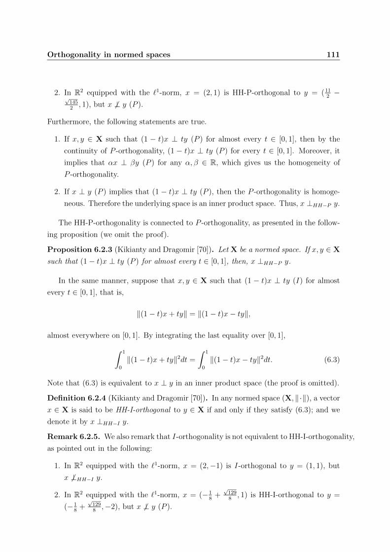
Orthogonality in normed spaces 111
2. In R2 equipped with the `1-norm, x = (2, 1) is HH-P-orthogonal to y = (112−
√1452, 1), but x 6⊥ y (P ).
Furthermore, the following statements are true.
1. If x, y ∈ X such that (1 − t)x ⊥ ty (P ) for almost every t ∈ [0, 1], then by the
continuity of P -orthogonality, (1 − t)x ⊥ ty (P ) for every t ∈ [0, 1]. Moreover, it
implies that αx ⊥ βy (P ) for any α, β ∈ R, which gives us the homogeneity of
P -orthogonality.
2. If x ⊥ y (P ) implies that (1 − t)x ⊥ ty (P ), then the P -orthogonality is homoge-
neous. Therefore the underlying space is an inner product space. Thus, x ⊥HH−P y.
The HH-P-orthogonality is connected to P -orthogonality, as presented in the follow-
ing proposition (we omit the proof).
Proposition 6.2.3 (Kikianty and Dragomir [70]). Let X be a normed space. If x, y ∈ X
such that (1− t)x ⊥ ty (P ) for almost every t ∈ [0, 1], then, x ⊥HH−P y.
In the same manner, suppose that x, y ∈ X such that (1 − t)x ⊥ ty (I) for almost
every t ∈ [0, 1], that is,
‖(1− t)x+ ty‖ = ‖(1− t)x− ty‖,
almost everywhere on [0, 1]. By integrating the last equality over [0, 1],∫ 1
0
‖(1− t)x+ ty‖2dt =
∫ 1
0
‖(1− t)x− ty‖2dt. (6.3)
Note that (6.3) is equivalent to x ⊥ y in an inner product space (the proof is omitted).
Definition 6.2.4 (Kikianty and Dragomir [70]). In any normed space (X, ‖·‖), a vector
x ∈ X is said to be HH-I-orthogonal to y ∈ X if and only if they satisfy (6.3); and we
denote it by x ⊥HH−I y.
Remark 6.2.5. We also remark that I-orthogonality is not equivalent to HH-I-orthogonality,
as pointed out in the following:
1. In R2 equipped with the `1-norm, x = (2,−1) is I-orthogonal to y = (1, 1), but
x 6⊥HH−I y.
2. In R2 equipped with the `1-norm, x = (−18
+√
1298, 1) is HH-I-orthogonal to y =
(−18
+√
1298,−2), but x 6⊥ y (P ).

112 Orthogonality in normed spaces
Furthermore, if x ⊥ y (I) implies that (1 − t)x ⊥ ty (I), then the I-orthogonality
is homogeneous. Therefore the underlying space is an inner product space. Thus,
x ⊥HH−I y.
Recall C-orthogonality, which is a generalization of P -orthogonality and I-orthogonality.
As the definition of HH-I-orthogonality arises from Proposition 6.2.3, we have the fol-
lowing definition, in the same manner.
Definition 6.2.6 (Kikianty and Dragomir [69]). Let m be a positive integer. In a
normed space (X, ‖ · ‖), x ∈ X is said to be HH-C-orthogonal to y ∈ X (we denote it
by x ⊥HH−C y) if and only if
m∑i=1
αi
∫ 1
0
‖(1− t)βix+ tγiy‖2 dt = 0, (6.4)
where αi, βi, γi are real numbers such that
m∑i=1
αiβ2i =
m∑i=1
αiγ2i = 0 and
m∑i=1
αiβiγi = 1. (6.5)
The main properties of this orthogonality are discussed in the subsequent sections.
Proposition 6.2.7 (Kikianty and Dragomir [69]). Let (X, 〈·, ·〉) be an inner product
space and x, y ∈ X. Then, x ⊥ y if and only if x ⊥HH−C y.
Proof. Let m be a positive integer. Since (X, 〈·, ·〉) is an inner product space, we have
m∑i=1
αi
∫ 1
0
‖(1− t)βix+ tγiy‖2 dt
=m∑i=1
αi
∫ 1
0
((1− t)2β2
i ‖x‖2 + 2t(1− t)βiγi〈x, y〉+ t2γ2i ‖y‖2
)dt
=1
3
(m∑i=1
αiβ2i ‖x‖2 +
m∑i=1
αiβiγi〈x, y〉+m∑i=1
αiγi‖y‖2
)=
1
3〈x, y〉,
by (6.5). If x ⊥ y, then 〈x, y〉 = 0. Therefore,
m∑i=1
αi
∫ 1
0
‖(1− t)βix+ tγiy‖2 dt = 0,

Orthogonality in normed spaces 113
that is, x ⊥HH−C y.
If x ⊥HH−C y, then
m∑i=1
αi
∫ 1
0
‖(1− t)βix+ tγiy‖2 dt =1
3〈x, y〉 = 0,
which implies that 〈x, y〉 = 0, that is, x ⊥ y.
Remark 6.2.8. Note that HH-P-orthogonality is a particular case of HH-C-orthogonality,
which is obtained by choosing m = 3, α1 = 1, α2 = α3 = −1, β1 = β2 = 1, β3 = 0,
γ1 = γ3 = 1 and γ2 = 0. Similarly, HH-I-orthogonality is also a particular case of HH-
C-orthogonality, which is obtained by choosing m = 2, α1 = 12, α2 = −1
2, β1 = β2 = 1,
γ1 = 1 and γ2 = −1.
Remark 6.2.9. Similarly to Remark 6.1.17, we consider some particular cases of HH-
C-orthogonality.
Let (X, ‖ · ‖) be a normed space and x, y ∈ X. Then,
1. x ⊥HH−S y if and only if ‖x‖‖y‖ = 0 or ‖x‖−1x ⊥HH−I ‖y‖−1y;
2. x ⊥HH−UP y if and only if ‖x‖‖y‖ = 0 or ‖x‖−1x ⊥HH−P ‖y‖−1y;
3. x ⊥HH−U y if and only if ‖x‖‖y‖ = 0 or ‖x‖−1x ⊥HH−C ‖y‖−1y;
4. x ⊥HH−aI y if and only if x ⊥HH−I ay for some fixed a 6= 0;
5. x ⊥HH−aP y if and only if x ⊥HH−P ay for some fixed a 6= 0;
6. x ⊥HH−ab y if and only if∫ 1
0
‖a(1− t)x+ bty‖2 + ‖(1− t)x+ ty‖2 dt
=
∫ 1
0
‖a(1− t)x+ ty‖2 + ‖(1− t)x+ bty‖2 dt
for some fixed a, b ∈ (0, 1);
7. x ⊥HH−a y if and only if (ax+ y) ⊥HH−P (x+ ay), for some fixed a 6= 1.
The properties of HH-C-orthogonality are considered in the following section. In particu-
lar, these properties hold for some special cases, namely, HH-P- and HH-I-orthogonalities
and those of Remark 6.2.9.

114 Orthogonality in normed spaces
6.3 Existence and main properties
The properties of HH-C-orthogonality are discussed in this section. The properties
of HH-P-orthogonality and HH-I-orthogonality follow by those of HH-C-orthogonality,
unless stated in special cases.
The following lemma covers the main properties of HH-C-orthogonality.
Lemma 6.3.1 (Kikianty and Dragomir [69]). HH-C-orthogonality satisfies the non-
degeneracy, simplification and continuity.
Proof. Let m be a positive integer. Suppose that x ⊥HH−C x, then
m∑i=1
αi
∫ 1
0
‖(1− t)βix+ tγix‖2 dt =m∑i=1
αi‖x‖2
∫ 1
0
|(1− t)βi + tγi|2 dt
=1
3‖x‖2
m∑i=1
αi(β2i + βiγi + γ2
i ) =1
3‖x‖2 = 0,
which implies that x = 0 (note the use of (6.5)). This shows that HH-C-orthogonality
is non-degenerate.
Suppose that x ⊥HH−C y and λ ∈ R. Then,
m∑i=1
αi
∫ 1
0
‖(1− t)βiλx+ tγiλy‖2 dt = |λ|2m∑i=1
αi
∫ 1
0
‖(1− t)βix+ tγiy‖2 dt = 0,
that is, λx ⊥HH−C λy, which proves the simplification property of HH-C-orthogonality.
If xn → x, yn → y and xn ⊥HH−C yn for any n ∈ N, then by continuity of the norm,
m∑i=1
αi
∫ 1
0
‖(1− t)βix+ tγiy‖2 dt
=m∑i=1
αi
∫ 1
0
∥∥(1− t)βi limn→∞
xn + tγi limn→∞
yn∥∥2
dt
= limn→∞
m∑i=1
αi
∫ 1
0
‖(1− t)βixn + tγiyn‖2 dt = 0,
that is, x ⊥HH−C y; and the continuity of HH-C-orthogonality is proven.

Orthogonality in normed spaces 115
With regards to symmetry, HH-C-orthogonality is symmetric in some cases, for ex-
ample, HH-P- and HH-I-orthogonalities are symmetric, as shown in the next proposition.
Proposition 6.3.2 (Kikianty and Dragomir [70]). Let X be a normed space. Then,
HH-P-orthogonality and HH-I-orthogonality are symmetric in X.
Proof. Let (X, ‖ · ‖) be a normed space and x, y ∈ X. If x ⊥HH−P y, then∫ 1
0
‖(1− t)y + tx‖2dt =
∫ 1
0
‖(1− t)x+ ty‖2dt
=1
3(‖x‖2 + ‖y‖2) =
1
3(‖y‖2 + ‖x‖2),
since the 2-HH-norm is symmetric. Hence, HH-P-orthogonality is symmetric. If x ⊥HH−Iy, then∫ 1
0
‖(1− t)y + tx‖2dt =
∫ 1
0
‖(1− t)x+ ty‖2dt
=
∫ 1
0
‖(1− t)x− ty‖2dt =
∫ 1
0
‖(1− t)y − tx‖2dt,
which proves that HH-I-orthogonality is symmetric.
The following provides an example of a nonsymmetric HH-C-orthogonality.
Example 6.3.3. Define x ⊥HH−C′ y to be∫ 1
0
‖(1− t)x+ 2ty‖2 dt =
∫ 1
0
‖(1− t)x− 2ty‖2 dt.
In the plane R2 with the `1-norm, x = (2, 1) is HH-C′-orthogonal to y = (12,−1) but
y 6⊥HH−C′ x.
Therefore, it is important to distinguish the existence (as well as the additivity) to the
left and to the right.
The following lemma is due to Carlsson [19, p. 299], which will be used in proving
the existence of HH-C-orthogonality.
Lemma 6.3.4 (Carlsson [19]). Let x, y ∈ X. Then,
limλ→±∞
λ−1[‖(λ+ a)x+ y‖2 − ‖λx+ y‖2
]= 2a‖x‖2.

116 Orthogonality in normed spaces
In the following theorem, it is shown that HH-C-orthogonality is existent to the left
and to the right. Hence, HH-P-orthogonality and HH-I-orthogonality are also existent.
In Section 6.6, alternative proofs for these cases are provided.
Theorem 6.3.5 (Kikianty and Dragomir [69]). Let (X, ‖ · ‖) be a normed space. Then,
HH-C-orthogonality is existent to the right and to the left.
Proof. The proof uses a similar idea to that of Carlsson [19, p. 301]. The proof is
provided for the existence to the right, as the other case follows analogously. Let m be
a positive integer and g be a function on R defined by
g(λ) :=m∑i=1
αi
∫ 1
0
‖(1− t)βix+ tγi(λx+ y)‖2 dt,
where αi, βi and γi are real numbers that satisfy (6.5). Note that our domain of integra-
tion is on (0, 1) (excluding the extremities) to ensure that we can employ Lemma 6.3.4.
Therefore, for any λ 6= 0,
λ−1g(λ) = λ−1
m∑i=1
αi
∫ 1
0
‖(1− t)βix+ tγi(λx+ y)‖2 dt (6.6)
= λ−1
m∑i=1
αi
∫ 1
0
[‖(1− t)βix+ tγi(λx+ y)‖2 − ‖tγi(λx+ y)‖2
]dt.
Note the use of∑m
i=1 αiγ2i = 0. Hence, (6.6) becomes
λ−1
[∑γi 6=0
αi
∫ 1
0
‖[tλ+ (1− t)βiγ−1i ]γix+ tγiy‖2 − ‖tλγix+ tγiy‖2 dt
+∑γi=0
αi
∫ 1
0
‖(1− t)βix‖2 dt
]
= λ−1
[∑γi 6=0
αi
∫ 1
0
‖[tλ+ (1− t)βiγ−1i ]γix+ tγiy‖2 − ‖tλγix+ tγiy‖2 dt
+1
3
∑γi=0
αiβ2i ‖x‖2
].
Note that
limλ→±∞
1
3λ−1
∑γi=0
αiβ2i ‖x‖2 = 0.

Orthogonality in normed spaces 117
By using Lemma 6.3.4, we obtain
limλ→±∞
λ−1g(λ) =∑γi 6=0
2αi
∫ 1
0
t(1− t)βiγ−1i ‖γix‖2 dt
=1
3
∑γi 6=0
αiβiγi‖x‖2 =1
3‖x‖2,
since∑m
i=1 αiβiγi = 1. It follows that g(λ) is positive for sufficiently large positive λ and
negative for sufficiently large negative λ. By the continuity of g, we conclude that there
exists a λ0 such that g(λ0) = 0, as required.
The following example shows that both HH-P-orthogonality and HH-I-orthogonality
are neither additive nor homogeneous.
Example 6.3.6. In R2 equipped with the `1-norm, set x = (0,−1) and y = (1, 3√
2−1).
Then, x ⊥HH−P y, but x 6⊥HH−P 2y. Again, in R2, with the `1-norm, x = (2, 1) is
HH-I-orthogonal to y = (1,−2), but x 6⊥HH−I 2y.
This example implies that HH-C-orthogonality is neither additive nor homogeneous.
We will discuss these properties further in Section 6.5 with regards to some characteri-
zations of an inner product space.
6.4 Uniqueness
In this section, we consider the uniqueness of HH-P-orthogonality and HH-I-orthogonality.
The uniqueness of HH-C-orthogonality in general will be discussed in Section 6.5.
The following lemma will be used to prove the uniqueness property of HH-P-orthogonality.
Lemma 6.4.1 (Kikianty and Dragomir [70]). Let (X, ‖ · ‖) be a normed space and
x, y ∈ X. Let g be a function on R defined by
g(k) :=
∫ 1
0
‖(1− t)y + k(tx)‖2 dt.
Then, g is a convex function on R and furthermore, for any s ∈ (0, 1) and k1, k2 ∈ Rwhere g(k1) 6= g(k2), we have
g[sk1 + (1− s)k2] < sg(k1) + (1− s)g(k2).

118 Orthogonality in normed spaces
Proof. The proof has a similar idea to that of Kapoor and Prasad in [68, p. 406]. Let
s ∈ (0, 1) and k1, k2 ∈ R, where k1 6= k2. Then,
g[sk1 + (1− s)k2]
=
∫ 1
0
‖(1− t)y + [sk1 + (1− s)k2](tx)‖2 dt (6.7)
=
∫ 1
0
‖s[(1− t)y + k1tx] + (1− s)[(1− t)y + k2tx]‖2 dt
≤ s2
∫ 1
0
‖(1− t)y + k1tx‖2 dt+ (1− s)2
∫ 1
0
‖(1− t)y + k2tx‖2 dt
+2s(1− s)∫ 1
0
‖(1− t)y + k1tx‖‖(1− t)y + k2tx‖ dt
= s
∫ 1
0
‖(1− t)y + k1tx‖2 dt+ (1− s)∫ 1
0
‖(1− t)y + k2tx‖2 dt
+(s2 − s)(∫ 1
0
‖(1− t)y + k1tx‖2 dt+
∫ 1
0
‖(1− t)y + k2tx‖2 dt
)+2s(1− s)
∫ 1
0
‖(1− t)y + k1tx‖‖(1− t)y + k2tx‖ dt
= s
∫ 1
0
‖(1− t)y + k1tx‖2 dt+ (1− s)∫ 1
0
‖(1− t)y + k2tx‖2 dt (6.8)
−s(1− s)(∫ 1
0
|‖(1− t)y + k1tx‖ − ‖(1− t)y + k2tx‖|2 dt)
≤ s
∫ 1
0
‖(1− t)y + k1tx‖2 dt+ (1− s)∫ 1
0
‖(1− t)y + k2tx‖2 dt
= sg(k1) + (1− s)g(k2).
Note that when equality holds, we conclude from (6.8) that∫ 1
0
|‖(1− t)y + k1tx‖ − ‖(1− t)y + k2tx‖|2 dt = 0,
that is, ‖(1− t)y+ k1tx‖ = ‖(1− t)y+ k2tx‖ almost everywhere on (0, 1), which implies
that
g(k1) =
∫ 1
0
|‖(1− t)y + k1tx‖2dt =
∫ 1
0
‖(1− t)y + k2tx‖2dt = g(k2).
Therefore, if g(k1) 6= g(k2), then the inequality is strict.
With this lemma in hand, we prove the uniqueness of HH-P-orthogonality, as pre-
sented in the next theorem.

Orthogonality in normed spaces 119
Theorem 6.4.2 (Kikianty and Dragomir [70]). Let X be a normed space. Then, HH-
P-orthogonality is unique on X.
Proof. The proof has a similar idea to that of Kapoor and Prasad in [68, p. 406].
Suppose that HH-P-orthogonality is not unique. Then there exist x, y ∈ X, x 6= 0 and
α > 0, such that
y ⊥HH−P x, (6.9)
and αx+ y ⊥HH−P x. (6.10)
Recall the convex function g as defined in Lemma 6.4.1. Observe that (6.9) implies that
g(0) =1
3‖y‖2,
and
g(1) =
∫ 1
0
‖(1− t)y + tx‖2 dt =‖y‖2
3+‖x‖2
3= g(0) +
‖x‖2
3. (6.11)
Set α′(t) = (1−t)αt
and observe that g(α′(t)) = 13‖αx+ y‖2, and
g(α′(t) + 1) =
∫ 1
0
‖(1− t)y + (α′(t) + 1)tx‖2 dt
=
∫ 1
0
‖(1− t)(αx+ y) + tx‖2 dt
=‖αx+ y‖2
3+‖x‖2
3= g(α′(t)) +
‖x‖2
3, (6.12)
by (6.10). Now, suppose that 0 < α′(t) < 1, and note that g(1) 6= g(0) (since x 6= 0).
Lemma 6.4.1 then gives us
g(α′(t)) < α′(t) g(1) + (1− α′(t)) g(0). (6.13)
Also, g(α′(t) + 1) 6= g(α′(t)) (since x 6= 0). By Lemma 6.4.1, we have
g(1) < α′(t) g(α′(t)) + (1− α′(t)) g(α′(t) + 1)
= α′(t) g(α′(t)) + (1− α′(t))[g(α′(t)) +
‖x‖2
3
]= α′(t) g(α′(t)) + (1− α′(t)) [g(α′(t)) + g(1)− g(0)] ,

120 Orthogonality in normed spaces
by (6.11) and (6.12). Therefore (by rearranging the last inequality), we have
α′(t)g(1) + (1− α′(t))g(0) < g(α′(t)),
which contradicts (6.13).
Now, consider the case that α′(t) > 1. We have,
g(1) ≤ α′(t)− 1
α′(t)g(0) +
1
α′(t)g(α′(t)),
that is,
‖x‖2
3= g(1)− g(0) ≤ 1
α′(t)[g(α′(t))− g(0)]. (6.14)
Since x 6= 0, (6.14) implies that g(α′(t)) 6= g(0). Thus, Lemma 6.4.1 gives us
g(1) <α′(t)− 1
α′(t)g(0) +
1
α′(t)g(α′(t)). (6.15)
Also, g(1) 6= g(α′(t) + 1) (since g(α′(t)) 6= g(0)) by (6.11) and (6.12). By employing
Lemma 6.4.1, we have
g(α′(t)) <1
α′(t)g(1) +
α′(t)− 1
α′(t)g(α′(t) + 1)
=1
α′(t)g(1) +
α′(t)− 1
α′(t)
[g(α′(t)) +
‖x‖2
3
]=
1
α′(t)g(1) +
α′(t)− 1
α′(t)[g(α′(t)) + g(1)− g(0)],
by (6.11) and (6.12). Therefore (by rearranging the last inequality), we have
1
α′(t)g(α′(t)) +
α′(t)− 1
α′(t)g(0) < g(1),
which contradicts (6.15). For the case where α′(t) = 1, we have
g(α′(t) + 1) = g(2) =‖x‖2
3+ g(1) = g(0) +
2‖x‖2
3.

Orthogonality in normed spaces 121
Again, note that g(0) 6= g(2) since x 6= 0; and Lemma 6.4.1 gives us
g(1) <1
2g(0) +
1
2g(2) = g(0) +
1
3‖x‖2
which contradicts (6.11). Therefore, HH-P-orthogonality must be unique.
The following lemma will be used to prove the uniqueness property of HH-I-orthogonality.
Lemma 6.4.3 (Kikianty and Dragomir [70]). Let (X, ‖ · ‖) be a strictly convex normed
space, x, y ∈ X and t ∈ (0, 1). Let g be a function on R defined by
g(k) :=
∫ 1
0
‖(1− t)y + k(tx)‖2 dt.
Then, g is a strictly convex function on R.
The proof follows readily from the fact that X is strictly convex. The details are omitted.
The uniqueness of HH-I-orthogonality is a characterization of strictly convex space,
as pointed out in the following theorem.
Theorem 6.4.4 (Kikianty and Dragomir [70]). Let (X, ‖ · ‖) be a normed space. Then,
HH-I-orthogonality is unique if and only if X is strictly convex.
Proof. The proof has a similar idea to that of Kapoor and Prasad in [68, p. 405].
Suppose that X is strictly convex and HH-I-orthogonality is not unique. Then, there
exist x, y ∈ X, where x 6= 0 and α > 0 such that
y ⊥HH−I x, and (6.16)
αx+ y ⊥HH−I x. (6.17)
Recall the strictly convex function g as defined in Lemma 6.4.3, for the given x, y and
t ∈ (0, 1) as follows
g(k) :=
∫ 1
0
‖(1− t)y + k(tx)‖2 dt.
Note that (6.16) gives us
g(1) =
∫ 1
0
‖(1− t)y + tx‖2 dt
=
∫ 1
0
‖(1− t)y − tx‖2 dt = g(−1).

122 Orthogonality in normed spaces
Set α′(t) = (1−t)αt
, t ∈ (0, 1), then
g(α′(t)− 1) =
∫ 1
0
‖(1− t)y + (α′(t)− 1)tx‖2 dt
=
∫ 1
0
‖(1− t)(αx+ y)− tx‖2 dt
=
∫ 1
0
‖(1− t)(αx+ y) + tx‖2 dt
=
∫ 1
0
‖(1− t)y + (α′(t) + 1)(tx)‖2 dt = g(α′(t) + 1),
from (6.17). Consider the case where 0 < α′(t) ≤ 2. We have
g(α′(t)− 1) = g
[(1− α′(t)
2
)(−1) +
α′(t)
2(1)
]<
(1− α′(t)
2
)g(−1) +
α′(t)
2g(1)
= g(1)
= g
[α′(t)
2(α′(t)− 1) +
(1− α′(t)
2
)(α′(t) + 1)
]<
α′(t)
2g (α′(t)− 1) +
(1− α′(t)
2
)g (α′(t) + 1)
= g(α′(t)− 1),
which leads us to a contradiction. Now consider the case where α′(t) > 2. The intervals
[−1, 1] and [α′(t) − 1, α′(t) + 1] are disjoint. Therefore, we have two distinct local
minimum, one on each of these intervals. But, g is strictly convex and thus can only
have one (global) minimum, which yields a contradiction.
Conversely, let us assume that X is not strictly convex. Let x, y ∈ X, x 6= y, such
that ‖x‖ = ‖y‖ = ‖x+y2‖ = 1. Then, the quantities
∫ 1
0
∥∥∥∥(1− t)x+ y
1− t
∥∥∥∥2
dt = ‖x+ y‖2,
∫ 1
0
∥∥∥∥(1− t)x+ y
1− t+ t
(x− yt
)∥∥∥∥2
dt = 4‖x‖2,
and ∫ 1
0
∥∥∥∥(1− t)x+ y
1− t− t(x− yt
)∥∥∥∥2
dt = 4‖y‖2,

Orthogonality in normed spaces 123
are all equal by our assumption.
Set x′ = x+y1−t and y′ = x−y
t, so we have
∫ 1
0
‖(1− t)x′‖2dt =
∫ 1
0
‖(1− t)x′ + ty′‖2dt (6.18)
=
∫ 1
0
‖(1− t)x′ − ty′‖2dt. (6.19)
Note that by (6.18), we have∫ 1
0
∥∥∥∥(1− t)(x′ +
ty′
2(1− t)
)+ t
(y′
2
)∥∥∥∥2
dt
=
∫ 1
0
‖(1− t)x′ + ty′‖2dt
=
∫ 1
0
‖(1− t)x′‖2dt
=
∫ 1
0
∥∥∥∥(1− t)(x′ +
ty′
2(1− t)
)− t(y′
2
)∥∥∥∥2
dt,
that is, [x′ +
t
1− t
(y′
2
)]⊥HH−I
(y′
2
). (6.20)
Also, by (6.19) we have ∫ 1
0
∥∥∥∥(1− t)(x′ − ty′
2(1− t)
)− t(y′
2
)∥∥∥∥2
dt
=
∫ 1
0
‖(1− t)x′ − ty′‖2dt
=
∫ 1
0
‖(1− t)x′‖2dt
=
∫ 1
0
∥∥∥∥(1− t)(x′ − ty′
2(1− t)
)+ t
(y′
2
)∥∥∥∥2
dt,
that is, [x′ − t
1− t
(y′
2
)]⊥HH−I
(y′
2
). (6.21)
By (6.20) and (6.21), we conclude that HH-I-orthogonality is not unique.

124 Orthogonality in normed spaces
6.5 Characterizations of inner product spaces
The main problem in the study of Banach space geometry is that most geometric prop-
erties fail to hold in a general normed space, unless it is an inner product space. The
characterization of inner product space has become an important area of research due
to this fact. Dan Amir has gathered numerous results concerning this field in his book
“Characterizations of inner product spaces” [5].
The main result of this section is a characterization of inner product space via
the homogeneity (and the additivity to the left) of HH-C-orthogonality (hence, HH-
P-orthogonality and HH-I-orthogonality).
Theorem 6.5.1 (Kikianty and Dragomir [69]). Let (X, ‖ · ‖) be a normed space in
which HH-C-orthogonality is homogeneous (or additive to the left). Then, X is an inner
product space.
It is important to note that since both HH-P-orthogonality and HH-I-orthogonality
are symmetric, Theorem 6.5.1 also holds for the additivity property to the right, in these
two cases. In Section 6.6, the alternative proofs for these cases are given.
The proof of this theorem is described in this section in two separate cases: the case
for normed space of dimension 3 and higher, and the 2-dimensional case. In both cases,
we consider a property introduced by Carlsson [19, p. 301], which is weaker than the
homogeneity and the additivity of the orthogonality (cf. Definition 6.1.23).
The following is a ‘modified’ definition of the property.
Definition 6.5.2 (Kikianty and Dragomir [69]). Let m be a positive integer. Then,
HH-C-orthogonality is said to have property (H) in a normed space X if x ⊥HH−C y
implies that
limn→∞
n−1
∫ 1
0
m∑i=1
αi‖nβi(1− t)x+ γity‖2 dt = 0. (6.22)
Note that
1. if HH-C-orthogonality is homogeneous (or additive to the left) in X, then it has
property (H);
2. if X is an inner product space, then HH-C-orthogonality is homogeneous (or addi-
tive), and therefore has property (H).

Orthogonality in normed spaces 125
Thus, in order to prove Theorem 6.5.1, it is sufficient to show that if the HH-C-
orthogonality has property (H) in X, then X is an inner product space.
The case of dimension 3 and higher
For the case of normed spaces with dimension 3 and higher, the proof of Theorem 6.5.1
follows by the fact that property (H) of HH-C-orthogonality implies that this orthog-
onality is symmetric and equivalent to B-orthogonality, whose proof will be described
in this subsection. Recall that the symmetry of B-orthogonality characterizes inner
product space of dimension 3 and higher (cf. Proposition 6.1.6).
The following propositions will be used to prove the theorem. We refer to Lemma
2.6. and Lemma 2.7. of Carlsson [19] for the proofs. Before stating the propositions, we
recall the following notation:
(∇+‖ · ‖(x))(y) := limt→0+
‖x+ ty‖ − ‖x‖t
and (∇−‖ · ‖(x))(y) := limt→0−
‖x+ ty‖ − ‖x‖t
x, y ∈ (X, ‖ · ‖)
that is, the right- and left-Gateaux derivatives at x ∈ X \ 0.
Proposition 6.5.3 (Carlsson [19]). Let (X, ‖ · ‖) be a normed space. Then, for λµ > 0
we have
(∇+‖ · ‖(λx))(µy) = |µ|(∇+‖ · ‖(x))(y),
and (∇−‖ · ‖(λx))(µy) = |µ|(∇−‖ · ‖(x))(y);
and for λµ < 0
(∇+‖ · ‖(λx))(µy) = −|µ|(∇−‖ · ‖(x))(y),
and (∇−‖ · ‖(λx))(µy) = −|µ|(∇+‖ · ‖(x))(y).
Proposition 6.5.4 (Carlsson [19]). Let (X, ‖ · ‖) be a normed linear space. If there
exist two real numbers λ and µ with λ+ µ 6= 0, such that
λ(∇+‖ · ‖(x))(y) + µ(∇−‖ · ‖(x))(y)
is a continuous function of x, y ∈ X, then the norm ‖ · ‖ is Gateaux differentiable.

126 Orthogonality in normed spaces
The following lemma will also be employed to prove Theorem 6.5.1 for the case of
normed spaces of dimension 3 and higher. This lemma also gives us the uniqueness of
HH-C-orthogonality.
Lemma 6.5.5 (Kikianty and Dragomir [69]). Let (X, ‖ · ‖) be a normed space where
HH-C-orthogonality has property (H). Suppose that for any x, y ∈ X, there exists λ ∈ Rsuch that x ⊥HH−C (λx+ y). Then,
λ = −‖x‖−1
[ ∑βiγi>0
αiβiγi(∇+‖ · ‖(x))(y) +∑βiγi<0
αiβiγi(∇−‖ · ‖(x))(y)
].
Proof. Suppose that m is a positive integer. By assumption, we have
limn→∞
n−1
∫ 1
0
m∑i=1
αi‖nβi(1− t)x+ γit(λx+ y)‖2 dt = 0. (6.23)
Note that by Lemma 6.3.4, we have the following for any i and t ∈ (0, 1) (again, note
that we exclude the extremities to ensure that we can employ Lemma 6.3.4)
n−1‖[nβi(1− t) + γitλ]x+ γity‖2 (6.24)
= n−1‖nβi(1− t)x+ γity‖2 + 2βi(1− t)γitλ‖x‖2 + εi(n),
where εi(n)→ 0 when n→ 0. Now, we multiply (6.24) by αi and integrate it over (0, 1),
to get
n−1αi
∫ 1
0
‖[nβi(1− t) + γitλ]x+ γity‖2 dt (6.25)
= n−1αi
∫ 1
0
‖nβi(1− t)x+ γity‖2 dt+ 2αiβiγiλ‖x‖2
∫ 1
0
(1− t)t dt+ εi(n).
Take the sum over i ∈ 1, . . . ,m and let n→∞ to get
0 = limn→∞
n−1
m∑i=1
αi
∫ 1
0
‖nβi(1− t)x+ γity‖2dt+1
3λ‖x‖2 (6.26)
(note the use of (6.25) and∑m
i=1 αiβiγi = 1).
Now, since∑m
i=1 αiβ2i = 0, then
n−1
m∑i=1
αi
∫ 1
0
‖nβi(1− t)x+ γity‖2dt

Orthogonality in normed spaces 127
= n−1
m∑i=1
αi
∫ 1
0
[‖nβi(1− t)x+ γity‖2 − ‖nβi(1− t)x‖2]dt
=m∑i=1
αi
∫ 1
0
[‖nβi(1− t)x+ γity‖ − ‖nβi(1− t)x‖]
× n−1[‖nβi(1− t)x+ γity‖+ ‖nβi(1− t)x‖]dt.
Rewrite
‖nβi(1− t)x+ γity‖ − ‖nβi(1− t)x‖
as
n(‖βi(1− t)x+ 1
nγity‖ − ‖βi(1− t)x‖
),
to obtain
limn→∞
n(‖βi(1− t)x+ 1
nγity‖ − ‖βi(1− t)x‖
)= lim
s→0+
‖βi(1− t)x+ sγity‖ − ‖βi(1− t)x‖s
= (∇+‖ · ‖(βi(1− t)x))(γity).
Note also that
limn→∞
n−1[‖nβi(1− t)x+ γity‖+ ‖nβi(1− t)x‖]
= limn→∞
[‖βi(1− t)x+ n−1γity‖+ ‖βi(1− t)x‖]
= 2‖βi(1− t)x‖.
Thus,
limn→∞
n−1
m∑i=1
αi
∫ 1
0
‖nβi(1− t)x+ γity‖2dt
= 2m∑i=1
αi
∫ 1
0
(∇+‖ · ‖(βi(1− t)x))(γity)‖βi(1− t)x‖dt.
Therefore,
λ = −3‖x‖−2
m∑i=1
αi
∫ 1
0
(∇+‖ · ‖(βi(1− t)x))(γity)2‖βi(1− t)x‖ dt
= −6‖x‖−1
m∑i=1
αi|βi|∫ 1
0
(1− t)τ+(βi(1− t)x, γity) dt.

128 Orthogonality in normed spaces
By Proposition 6.5.3, (6.26) gives us
λ = −6‖x‖−1
∫ 1
0
(1− t)t dt
×
[ ∑βiγi>0
αiβiγi(∇+‖ · ‖(x))(y) +∑βiγi<0
αiβiγi(∇−‖ · ‖(x))(y)
]
= −‖x‖−1
[ ∑βiγi>0
αiβiγi(∇+‖ · ‖(x))(y) +∑βiγi<0
αiβiγi(∇−‖ · ‖(x))(y)
].
This completes the proof.
Now, we have a unique λ for any x, y ∈ X such that x ⊥HH−C λx+ y. As a function
of x and y, λ = λ(x, y) is a continuous function [19, p. 303]. Thus,∑βiγi>0
αiβiγi(∇+‖ · ‖(x))(y) +∑βiγi<0
αiβiγi(∇−‖ · ‖(x))(y)
is also a continuous function in x, y ∈ X. By Proposition 6.5.4, the norm ‖·‖ is Gateaux
differentiable. Hence, we have the following consequence.
Corollary 6.5.6 (Kikianty and Dragomir [69]). If HH-C-orthogonality has property
(H), then the norm of X is Gateaux differentiable and x ⊥HH−C y holds if and only if
(∇‖ · ‖(x))(y) = 0, that is, x ⊥ y (B).
Remark 6.5.7. We note that the function (∇‖·‖(x))(y) is also continuous as a function
of x and y.
Let us assume that x is HH-C-anti-orthogonal to y if and only if y ⊥HH−C x. We
have shown that when HH-C-orthogonality has property (H), then it is equivalent to
B-orthogonality and therefore is homogeneous (since B-orthogonality is homogeneous).
This fact implies that HH-C-anti-orthogonality has property (H), as the homogeneity
property implies property (H). Therefore, the above results also hold for HH-C-anti-
orthogonality. In particular, (∇‖ · ‖(x))(y) = 0 implies that x ⊥HH−C y, that is, y
is HH-C-anti-orthogonal to x. Hence, (∇‖ · ‖(y))(x) = 0. Thus, B-orthogonality is
symmetric; and we obtain the following consequence.
Corollary 6.5.8 (Kikianty and Dragomir [69]). If HH-C-orthogonality has property
(H), then it is symmetric and equivalent to B-orthogonality.
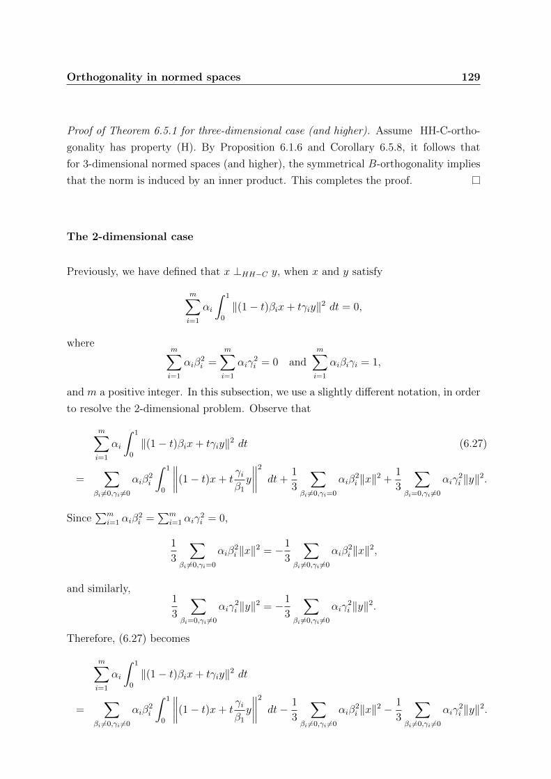
Orthogonality in normed spaces 129
Proof of Theorem 6.5.1 for three-dimensional case (and higher). Assume HH-C-ortho-
gonality has property (H). By Proposition 6.1.6 and Corollary 6.5.8, it follows that
for 3-dimensional normed spaces (and higher), the symmetrical B-orthogonality implies
that the norm is induced by an inner product. This completes the proof.
The 2-dimensional case
Previously, we have defined that x ⊥HH−C y, when x and y satisfy
m∑i=1
αi
∫ 1
0
‖(1− t)βix+ tγiy‖2 dt = 0,
wherem∑i=1
αiβ2i =
m∑i=1
αiγ2i = 0 and
m∑i=1
αiβiγi = 1,
and m a positive integer. In this subsection, we use a slightly different notation, in order
to resolve the 2-dimensional problem. Observe that
m∑i=1
αi
∫ 1
0
‖(1− t)βix+ tγiy‖2 dt (6.27)
=∑
βi 6=0,γi 6=0
αiβ2i
∫ 1
0
∥∥∥∥(1− t)x+ tγiβ1
y
∥∥∥∥2
dt+1
3
∑βi 6=0,γi=0
αiβ2i ‖x‖2 +
1
3
∑βi=0,γi 6=0
αiγ2i ‖y‖2.
Since∑m
i=1 αiβ2i =
∑mi=1 αiγ
2i = 0,
1
3
∑βi 6=0,γi=0
αiβ2i ‖x‖2 = −1
3
∑βi 6=0,γi 6=0
αiβ2i ‖x‖2,
and similarly,1
3
∑βi=0,γi 6=0
αiγ2i ‖y‖2 = −1
3
∑βi 6=0,γi 6=0
αiγ2i ‖y‖2.
Therefore, (6.27) becomes
m∑i=1
αi
∫ 1
0
‖(1− t)βix+ tγiy‖2 dt
=∑
βi 6=0,γi 6=0
αiβ2i
∫ 1
0
∥∥∥∥(1− t)x+ tγiβ1
y
∥∥∥∥2
dt− 1
3
∑βi 6=0,γi 6=0
αiβ2i ‖x‖2 − 1
3
∑βi 6=0,γi 6=0
αiγ2i ‖y‖2.

130 Orthogonality in normed spaces
We set pi = αiβ2i and qi = γi/βi and rearrange the indices to obtain
m∑i=1
αi
∫ 1
0
‖(1− t)βix+ tγiy‖2 dt (6.28)
=r∑
k=1
pk
∫ 1
0
‖(1− t)x+ tqky‖2 dt− 1
3
r∑k=1
pk‖x‖2 − 1
3
r∑k=1
pkq2k‖y‖2.
Assume that HH-C-orthogonality has property (H). Then, it is equivalent to B-
orthogonality, and therefore is homogeneous. Denote SX to be the unit circle in X with
respect to the norm ‖ · ‖ and let x, y ∈ SX such that x ⊥HH−C y. Then, (6.28) gives us
3r∑
k=1
pk
∫ 1
0
‖(1− t)x+ tqkαy‖2 dt = C1 + C2α2,
where C1 =∑r
k=1 pk and C2 =∑r
k=1 pkq2k. We may conclude that the function
φ(α) = 3
∫ 1
0
‖(1− t)x+ tαy‖2 dt
is the solution of the functional equation
r∑k=1
pkF (qkα) = C1 + C2α2, −∞ < α <∞, (6.29)
where
r∑k=1
pk = C1,r∑
k=1
pkq2k = C2,
r∑k=1
pkqk = 1, qk 6= 0, k = 1, . . . , r. (6.30)
We note that the function φ is continuously differentiable from Corollary 6.5.6 and
Remark 6.5.7.
In the following results by Carlsson [19], it is shown that the behaviour of φ for large
and small values of |α| gives us an explicit formula for φ.
Definition 6.5.9 (Carlsson [19]). Let r and s be two positive integers. Given a func-
tional equationr∑
k=1
pkF (qkα) = C1 + C2α2, −∞ < α <∞,

Orthogonality in normed spaces 131
for some real numbers C1, C2, pk and qk. We say that the equation is symmetric if it
can be written in the form
s∑k=1
mkF (nkα)−s∑
k=1
mkF (−nkα) = C1 + C2α2
for some real numbers C1, C2, mk and nk; otherwise, it is nonsymmetric.
Lemma 6.5.10 (Carlsson [19]). Let φ(α) be a continuously differentiable solution of the
functional equation (6.29) satisfying (6.30) and
φ(α) = 1 +O(α2) when α→ 0
φ(α) = α2 +O(α) when α→ ±∞.
If (6.29) is nonsymmetric, then φ(α) = 1 + α2 for −∞ < α <∞. If (6.29) is (nontriv-
ially) symmetric, then φ(α) = φ(−α) for −∞ < α <∞.
A 2-dimensional normed space has certain properties that enable us to work on a
smaller subset. One of the useful properties is stated in Lemma 6.5.11. Before stating
the lemma, recall that the norm ‖ · ‖ : X → R is said to be Frechet differentiable (or,
differentiable) at x ∈ X if and only if there exists a continuous linear functional ϕ′x on
X such that
lim‖z‖→0
|‖x+ z‖ − ‖x‖ − ϕ′x(z)|‖z‖
= 0.
It is said to be twice (Frechet) differentiable at x ∈ X if and only if there exists a
continuous bilinear functional ϕ′′x on X2 such that
lim‖z‖→0
|‖x+ z‖ − ‖x‖ − ϕ′x(z)− ϕ′′x(z, z)|‖z‖2
= 0.
Lemma 6.5.11 (Amir [5]). If (X, ‖·‖) is a 2-dimensional normed space, then the norm
is twice (Frechet) differentiable almost everywhere on the unit circle SX = u ∈ X :
‖u‖ = 1.
This result follows by the fact that the direction of the left-side tangent is a monotone
function and therefore, by Lebesgue’s theorem, is differentiable almost everywhere [5, p.
22].

132 Orthogonality in normed spaces
By assuming that HH-C-orthogonality is homogeneous, we may restrict ourself to
work on the unit circle. Furthermore, the previous proposition enables us to work on a
dense subset of the unit circle.
Proof of Theorem 6.5.1 for 2-dimensional case. Assume HH-C-orthogonality has prop-
erty (H). Then, it is equivalent to B-orthogonality, and therefore is homogeneous. Since
dim(X) = 2, then the norm ‖ · ‖ is twice differentiable for almost every u ∈ SX.
Let D be the subset of SX consists of all points where the norm ‖ · ‖ is twice differ-
entiable. Let x ∈ D and x ⊥HH−C y (or, equivalently x ⊥ y (B)) with ‖y‖ = 1. Then,
the function
φ(α) = 3
∫ 1
0
‖(1− t)x+ tαy‖2 dt
is a continuously differentiable solution of the functional equation (6.29) satisfying (6.30).
Claim 6.5.12. The function φ satisfies
φ(α) = 1 +O(α2) when α→ 0
φ(α) = α2 +O(α) when α→ ±∞.
The proof of this claim will be stated at the end of this section as Lemmas 6.5.13 and
6.5.14.
Case 1: Equation (6.30) is nonsymmetric. It follows from Lemma 6.5.10 that φ(α) =
1 + α2. If we choose x and y as the unit vectors of a coordinate system in the plane X
and write w = νx+ ηy, we see that ‖w‖ = 1 if and only if ν2 + η2 = 1. This means that
the unit circle has the equation ν2 + η2 = 1, that is, an Euclidean circle. Therefore, X
is an inner product space.
Case 2: Equation (6.30) is symmetric. It follows from Lemma 6.5.10 that φ(α) = φ(−α)
for all α, that is, ∫ 1
0
‖(1− t)x+ tαy‖2 dt =
∫ 1
0
‖(1− t)x− tαy‖2 dt (6.31)
holds for any α ∈ R, x, y ∈ X where x ∈ D and x ⊥HH−C y.
Since D is a dense subset of C and HH-C-orthogonality is homogeneous, we conclude
that (6.31) also holds for any x ∈ X where x ⊥HH−C y. Let t ∈ (0, 1) and for any β ∈ R,

Orthogonality in normed spaces 133
choose α = (1−t)tβ. Then, (6.31) gives us∫ 1
0
‖(1− t)x+ (1− t)βy‖2 dt =
∫ 1
0
‖(1− t)x− (1− t)βy‖2 dt,
or equivalently
‖x+ βy‖ = ‖x− βy‖,
that is, x ⊥ y (R). Thus, HH-C-orthogonality implies R-orthogonality. Since HH-C-
orthogonality is existent, X is an inner product space by Proposition 6.1.27.
The proof of claim is stated as the following lemmas:
Lemma 6.5.13 (Kikianty and Dragomir [69]). Suppose that (X, ‖·‖) be a 2-dimensional
normed space and denote its unit circle by SX. Let u, v ∈ SX. Then, the function
φ(α) = 3
∫ 1
0
‖(1− t)u+ tαv‖2 dt
satisfies the condition
φ(α) = α2 +O(α) when α→ ±∞.
Proof. For any u, v ∈ SX and α ∈ R, we have
|φ(α)− α2|
=
∣∣∣∣3(∫ 1
0
‖(1− t)u+ tαv‖2 dt− 1
3α2
)∣∣∣∣=
∣∣∣∣3∫ 1
0
‖(1− t)u+ tαv‖2 − ‖tαv‖2 dt
∣∣∣∣≤ 3
∫ 1
0
∣∣∣∣ ‖(1− t)u+ tαv‖2 − ‖tαv‖2
∣∣∣∣ dt= 3
∫ 1
0
∣∣∣∣ ‖(1− t)u+ tαv‖ − ‖tαv‖∣∣∣∣( ‖(1− t)u+ tαv‖+ ‖tαv‖
)dt
≤ 3
∫ 1
0
(1− t) ‖u‖(
(1− t)‖u‖+ 2t‖αv‖)dt
= 3
∫ 1
0
((1− t)2 + 2t(1− t)|α|) dt = 1 + |α|.
Thus, φ(α)− α2 = O(α), when α→ ±∞.

134 Orthogonality in normed spaces
Lemma 6.5.14 (Kikianty and Dragomir [69]). Let (X, ‖ ·‖) be a 2-dimensional normed
space and denote its unit circle by SX. Then, there is a dense subset D of SX such that
if u ∈ D and u ⊥ v (B), the function
φ(α) = 3
∫ 1
0
‖(1− t)u+ tαv‖2 dt
satisfies
φ(α) = 1 +O(α2) when α→ 0. (6.32)
Proof. Since dim(X) = 2, then the norm ‖ · ‖ is twice differentiable for almost every
u ∈ SX by Lemma 6.5.11 [5, p. 22]. Let D be the subset of SX consists of all points
where the norm ‖ · ‖ is twice differentiable. We conclude that D is a dense subset of SX.
Denote ϕ(x) = ‖x‖, then for any u ∈ D, the derivative ϕ′u is a linear functional and the
second derivative ϕ′′u is a bilinear functional. Furthermore, we have
lim‖z‖→0
∣∣∣∣‖u+ z‖ − ‖u‖ − ϕ′u(z)− ϕ′′u(z, z)
‖z‖2
∣∣∣∣ = 0. (6.33)
Let u ∈ D and u ⊥ v (B), where ‖v‖ = 1. Set z = t1−tαv (t ∈ (0, 1)). Therefore,
when α→ 0, ‖z‖ → 0. Since u ⊥ v (B), ϕ′u(v) = 0; and (6.33) gives us
limα→0
∣∣∣∣∣∥∥u+
(t
1−tα)v∥∥− ‖u‖ − ( t
1−tα)2ϕ′′u(v, v)(
t1−tα
)2 ‖v‖2
∣∣∣∣∣ = 0,
that is, for any ε > 0, there exists δ0 > 0, such that for any |α| < δ0, we have∣∣∣∣∣∥∥u+
(t
1−tα)v∥∥− 1(
t1−tα
)2 − ϕ′′u(v, v)
∣∣∣∣∣ < ε.
Furthermore, by triangle inequality, we obtain∣∣∣∣∣∣∥∥∥u+ t
(1−t)αv∥∥∥− 1
t2
(1−t)2α2
∣∣∣∣∣∣ < ε+ |ϕ′′u(v, v)| = M.
Equivalently, we have, ∣∣∣∣∥∥∥∥u+t
1− tαv
∥∥∥∥− 1
∣∣∣∣ < Mt2
(1− t)2α2.

Orthogonality in normed spaces 135
Note that for any t ∈ (0, 1),∥∥u+ 1−t
tαv∥∥+ 1→ 2 when α→ 0. It can be shown that
there exists δ1 such that for any |α| < δ1, we have∣∣∣∣∥∥∥∥u+t
1− tαv
∥∥∥∥+ 1− 2
∣∣∣∣ < 1,
that is, ∥∥∥∥u+t
1− tαv
∥∥∥∥+ 1 < 1 + 2 = 3.
Now, for any |α| < minδ0, δ1, we have
|φ(α)− 1| =
∣∣∣∣3(∫ 1
0
‖(1− t)u+ tαv‖2 dt− 1
3
)∣∣∣∣=
∣∣∣∣3∫ 1
0
‖(1− t)u+ tαv‖2 − ‖(1− t)u‖2 dt
∣∣∣∣≤ 3
∫ 1
0
∣∣∣∣ ‖(1− t)u+ tαv‖2 − ‖(1− t)u‖2
∣∣∣∣ dt= 3
∫ 1
0
(1− t)2
∣∣∣∣ ∥∥∥∥u+t
1− tαv
∥∥∥∥2
− ‖u‖2
∣∣∣∣ dt= 3
∫ 1
0
(1− t)2
(∥∥∥∥u+t
1− tαv
∥∥∥∥+ 1
)∣∣∣∣ ∥∥∥∥u+t
1− tαv
∥∥∥∥− 1
∣∣∣∣ dt< 9
∫ 1
0
(1− t)2Mt2
(1− t)2α2 dt = 3Mα2,
that is, φ(α)− 1 = O(α2), when α→ 0.
The last results conclude that the homogeneity (also, the right-additivity) of HH-C-
orthogonality is a necessary and sufficient condition for the normed space to be an inner
product space.
6.6 Alternative proofs for special cases
In this section, alternative proofs for the existence and characterization of inner product
spaces via the homogeneity and the additivity properties, are provided in particular
settings of HH-P-orthogonality and HH-I-orthogonality.

136 Orthogonality in normed spaces
6.6.1 Existence
The following theorem gives us the existence of HH-P-orthogonality. The proof for the
existence property employs the similar continuity argument and the intermediate value
theorem, which was used by James [61, p. 299–300].
Theorem 6.6.1 (Kikianty and Dragomir [70]). Let (X, ‖ · ‖) be a normed space. Then,
HH-P-orthogonality is existent.
Proof. Fix x, y ∈ X. The proof is trivial when x = 0, thus, we assume that x 6= 0.
Let f : R× (0, 1)→ R be a function defined by
f(α, t) := t2‖x‖2 + (1− t)2‖(αx+ y)‖2 − ‖(1− t)(αx+ y) + tx‖2, (6.34)
and F be a function on R defined by F (α) :=∫ 1
0f(α, t) dt.
Note that when F (α) = 0, we have
‖x‖2
∫ 1
0
t2dt+ ‖(αx+ y)‖2
∫ 1
0
(1− t)2dt−∫ 1
0
‖(1− t)(αx+ y) + tx‖2dt = 0,
which is equivalent to∫ 1
0
‖(1− t)(αx+ y) + tx‖2dt =1
3
(‖(αx+ y)‖2 + ‖x‖2
),
that is, (αx + y) ⊥HH−C x. To show that there exists an α such that the continuous
function F is zero, we apply the intermediate value theorem to show that there exist
two distinct α1 and α2 such that F (α1) < 0 and F (α2) > 0.
Let α > 0. Since t 6= 1, we have the following identity
1 = −2t(1− t)α + t2
(1− t)2α2+
((1− t)α + t
(1− t)α
)2
.
We have
f(α, t) = t2‖x‖2 − 2t(1− t)α + t2
(1− t)2α2(1− t)2‖αx+ y‖2
+
((1− t)α + t
(1− t)α
)2
(1− t)2‖αx+ y‖2 − ‖[(1− t)α + t]x+ (1− t)y‖2

Orthogonality in normed spaces 137
= t2‖x‖2 −[2t(1− t)α + t2
] ∥∥∥x+y
α
∥∥∥2
+
∥∥∥∥[(1− t)α + t]x+
[(1− t) +
t
α
]y
∥∥∥∥2
− ‖[(1− t)α + t]x+ (1− t)y‖2
= t2‖x‖2 −[2t(1− t)α + t2
] ∥∥∥x+y
α
∥∥∥2
+
[∥∥∥∥[(1− t)α + t]x+
[(1− t) +
t
α
]y
∥∥∥∥− ‖[(1− t)α + t]x+ (1− t)y‖]
×[∥∥∥∥[(1− t)α + t]x+
[(1− t) +
t
α
]y
∥∥∥∥+ ‖[(1− t)α + t]x+ (1− t)y‖].
Note that by the triangle inequality, we have[∥∥∥∥[(1− t)α + t]x+
[(1− t) +
t
α
]y
∥∥∥∥− ‖[(1− t)α + t]x+ (1− t)y‖]
≤∣∣∣∣ tα∣∣∣∣ ‖y‖ =
t
α‖y‖,
since α > 0. Again, by the triangle inequality,[∥∥∥∥[(1− t)α + t]x+
[(1− t) +
t
α
]y
∥∥∥∥+ ‖[(1− t)α + t]x+ (1− t)y‖]
≤ 2|(1− t)α + t|‖x‖+
[∣∣∣∣(1− t) +t
α
∣∣∣∣+ (1− t)]‖y‖
= 2[(1− t)α + t]‖x‖+
[2(1− t) +
t
α
]‖y‖.
Therefore,
f(α, t)
≤ t2‖x‖2 −[2t(1− t)α + t2
] ∥∥∥x+y
α
∥∥∥2
+
(2t(1− t) +
2t2
α
)‖x‖‖y‖+
[2t(1− t)
α+t2
α2
]‖y‖2
≤ t2‖x‖2 −[2t(1− t)α + t2
] (‖x‖ −
∥∥∥ yα
∥∥∥)2
+
(2t(1− t) +
2t2
α
)‖x‖‖y‖+
[2t(1− t)
α+t2
α2
]‖y‖2
= t2‖x‖2 −[2t(1− t)α + t2
]‖x‖2
+2[2t(1− t)α + t2
]‖x‖
∥∥∥ yα
∥∥∥− [2t(1− t)α + t2] ∥∥∥ yα
∥∥∥2
+
(2t(1− t) +
2t2
α
)‖x‖‖y‖+
[2t(1− t)
α+t2
α2
]‖y‖2

138 Orthogonality in normed spaces
= −2t(1− t)α‖x‖2 +
[4t(1− t) +
2t2
α
]‖x‖‖y‖ −
[2t(1− t)
α+t2
α2
]‖y‖2
+
(2t(1− t) +
2t2
α
)‖x‖‖y‖+
[2t(1− t)
α+t2
α2
]‖y‖2
= −2t(1− t)α‖x‖2 +
[6t(1− t) +
4t2
α
]‖x‖‖y‖.
Integrate the last inequality with respect to t on (0, 1) to get
F (α) =
∫ 1
0
f(α, t)dt
≤∫ 1
0
(−2t(1− t)α‖x‖2 +
[6t(1− t) +
4t2
α
]‖x‖‖y‖
)dt
= −1
3α‖x‖2 +
[1 +
4
3α
]‖x‖‖y‖.
By taking α sufficiently large (denote this value by α1) and since x is nonzero, we have
F (α1) =
∫ 1
0
f(α1, t)dt < 0.
Again, let α > 0, we have
f(−α, t) = t2‖x‖2 + (1− t)2‖αx− y‖2 − ‖(1− t)(αx− y)− tx‖2.
Since t 6= 1, we have the following identity
1 =2t(1− t)α− t2
(1− t)2α2+
((1− t)α− t
(1− t)α
)2
.
Thus, we have the following
f(−α, t) = t2‖x‖2 +2t(1− t)α− t2
(1− t)2α2(1− t)2‖αx− y‖2
+
((1− t)α− t
(1− t)α
)2
(1− t)2‖αx− y‖2 − ‖[(1− t)α− t]x− (1− t)y‖2
= t2‖x‖2 + [2t(1− t)α− t2]∥∥∥x− y
α
∥∥∥2
+
∥∥∥∥[(1− t)α− t]x−(
1− t− t
α
)y
∥∥∥∥2
− ‖[(1− t)α− t]x− (1− t)y‖2

Orthogonality in normed spaces 139
= t2‖x‖2 + [2t(1− t)α− t2]∥∥∥x− y
α
∥∥∥2
+
[∥∥∥∥[(1− t)α− t]x−(
1− t− t
α
)y
∥∥∥∥− ‖[(1− t)α− t]x− (1− t)y‖]
×[∥∥∥∥[(1− t)α− t]x−
(1− t− t
α
)y
∥∥∥∥+ ‖[(1− t)α− t]x− (1− t)y‖].
By the triangle inequality, we have[∥∥∥∥[(1− t)α− t]x−(
1− t− t
α
)y
∥∥∥∥− ‖[(1− t)α− t]x− (1− t)y‖]
≥ −∣∣∣∣ tα∣∣∣∣ ‖y‖ = − t
α‖y‖.
Again, by the triangle inequality, we also have[∥∥∥∥[(1− t)α− t]x−(
1− t− t
α
)y
∥∥∥∥+ ‖[(1− t)α− t]x− (1− t)y‖]
≤[2|(1− t)α− t| ‖x‖+
[∣∣∣∣1− t− t
α
∣∣∣∣+ 1− t]‖y‖].
Therefore,
f(−α, t) ≥ t2‖x‖2 + 2t(1− t)α∥∥∥x− y
α
∥∥∥2
− t2∥∥∥x− y
α
∥∥∥2
−2
∣∣∣∣(1− t)t− t2
α
∣∣∣∣ ‖x‖ ‖y‖ − [∣∣∣∣t(1− t)α− t2
α2
∣∣∣∣+(1− t)t
α
]‖y‖2
≥ t2‖x‖2 + 2t(1− t)α∥∥∥x− y
α
∥∥∥2
− t2(‖x‖+
∥∥∥ yα
∥∥∥)2
−2
∣∣∣∣(1− t)t− t2
α
∣∣∣∣ ‖x‖ ‖y‖ − [∣∣∣∣t(1− t)α− t2
α2
∣∣∣∣+(1− t)t
α
]‖y‖2
= t2‖x‖2 + 2t(1− t)α∥∥∥x− y
α
∥∥∥2
− t2‖x‖2 − 2t2‖x‖∥∥∥ yα
∥∥∥− t2 ∥∥∥ yα
∥∥∥2
−2
∣∣∣∣(1− t)t− t2
α
∣∣∣∣ ‖x‖ ‖y‖ − [∣∣∣∣t(1− t)α− t2
α2
∣∣∣∣+
∣∣∣∣(1− t)tα
∣∣∣∣] ‖y‖2
= 2t(1− t)α∥∥∥x− y
α
∥∥∥2
−[2
∣∣∣∣(1− t)t− t2
α
∣∣∣∣+2t2
α
]‖x‖ ‖y‖
−[∣∣∣∣t(1− t)α
− t2
α2
∣∣∣∣+(1− t)t
α+t2
α2
]‖y‖2
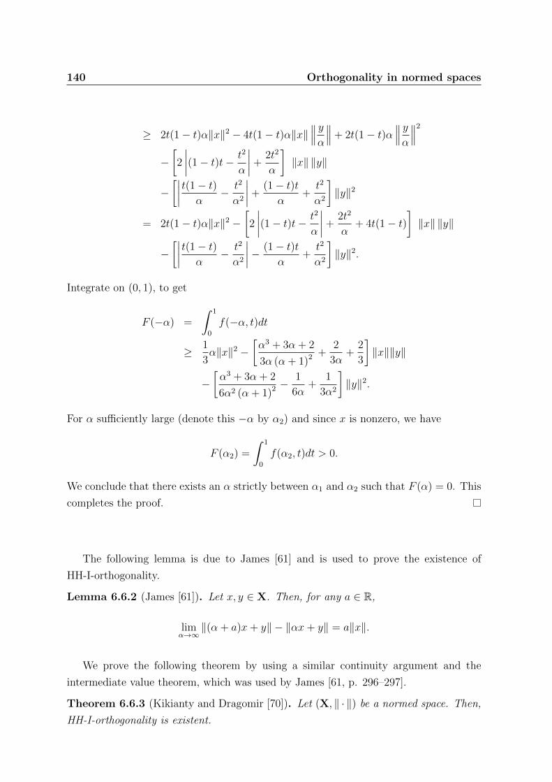
140 Orthogonality in normed spaces
≥ 2t(1− t)α‖x‖2 − 4t(1− t)α‖x‖∥∥∥ yα
∥∥∥+ 2t(1− t)α∥∥∥ yα
∥∥∥2
−[2
∣∣∣∣(1− t)t− t2
α
∣∣∣∣+2t2
α
]‖x‖ ‖y‖
−[∣∣∣∣t(1− t)α
− t2
α2
∣∣∣∣+(1− t)t
α+t2
α2
]‖y‖2
= 2t(1− t)α‖x‖2 −[2
∣∣∣∣(1− t)t− t2
α
∣∣∣∣+2t2
α+ 4t(1− t)
]‖x‖ ‖y‖
−[∣∣∣∣t(1− t)α
− t2
α2
∣∣∣∣− (1− t)tα
+t2
α2
]‖y‖2.
Integrate on (0, 1), to get
F (−α) =
∫ 1
0
f(−α, t)dt
≥ 1
3α‖x‖2 −
[α3 + 3α + 2
3α (α + 1)2 +2
3α+
2
3
]‖x‖‖y‖
−[α3 + 3α + 2
6α2 (α + 1)2 −1
6α+
1
3α2
]‖y‖2.
For α sufficiently large (denote this −α by α2) and since x is nonzero, we have
F (α2) =
∫ 1
0
f(α2, t)dt > 0.
We conclude that there exists an α strictly between α1 and α2 such that F (α) = 0. This
completes the proof.
The following lemma is due to James [61] and is used to prove the existence of
HH-I-orthogonality.
Lemma 6.6.2 (James [61]). Let x, y ∈ X. Then, for any a ∈ R,
limα→∞
‖(α + a)x+ y‖ − ‖αx+ y‖ = a‖x‖.
We prove the following theorem by using a similar continuity argument and the
intermediate value theorem, which was used by James [61, p. 296–297].
Theorem 6.6.3 (Kikianty and Dragomir [70]). Let (X, ‖ · ‖) be a normed space. Then,
HH-I-orthogonality is existent.

Orthogonality in normed spaces 141
Proof. Let x, y ∈ X. The proof is trivial for x = 0. Therefore, we assume that x 6= 0.
Suppose that h : R× (0, 1)→ R be a function defined by
h(α, t) := ‖(1− t)(αx+ y) + tx‖ − ‖(1− t)(αx+ y)− tx‖
= ‖[(1− t)α + t]x+ (1− t)y‖ − ‖[(1− t)α− t]x+ (1− t)y‖,
and associated to h, a function H : R→ R defined by
H(α) :=
∫ 1
0
h(α, t)dt.
Note that, for any t ∈ (0, 1),
limα→∞
h(α, t) = limα→∞
[‖[(1− t)α + t]x+ (1− t)y‖ − ‖[(1− t)α− t]x+ (1− t)y‖
]= (1− t) lim
α→∞
[∥∥∥∥(α +t
1− t
)x+ y
∥∥∥∥− ∥∥∥∥(α− t
1− t
)x+ y
∥∥∥∥]= (1− t) lim
α→∞
[∥∥∥∥(α +2t
1− t
)x+ y
∥∥∥∥− ‖αx+ y‖]
= (1− t) 2t
(1− t)‖x‖ = 2t‖x‖,
by Lemma 6.6.2, and that
limα→∞
H(α) = limα→∞
∫ 1
0
h(α, t) dt =
∫ 1
0
limα→∞
h(α, t) dt,
by the continuity of h. Therefore,
limα→∞
H(α) =
∫ 1
0
2t‖x‖ dt = ‖x‖ > 0.
We also note that for any t ∈ (0, 1)
limα→∞
h(−α, t)
= limα→∞
[‖[(1− t)(−α) + t]x+ (1− t)y‖ − ‖[(1− t)(−α)− t]x+ (1− t)y‖
]= lim
α→∞
[‖[(1− t)α− t]x− (1− t)y‖ − ‖[(1− t)α + t]x− (1− t)y‖
]= (1− t) lim
α→∞
[∥∥∥∥(α− t
1− t
)x− y
∥∥∥∥− ∥∥∥∥(α +t
1− t
)x− y
∥∥∥∥]

142 Orthogonality in normed spaces
= (1− t) limα→∞
[∥∥∥∥(α− 2t
1− t
)x− y
∥∥∥∥− ‖αx− y‖]= (1− t)
(− 2t
1− t
)‖x‖ = −2t‖x‖,
again by Lemma 6.6.2, and by the continuity of h,
limα→∞
H(−α) = limα→∞
∫ 1
0
h(−α, t) dt =
∫ 1
0
limα→∞
h(−α, t) dt.
Therefore,
limα→∞
H(−α) =
∫ 1
0
(−2t)‖x‖ dt = −‖x‖ < 0.
Now, we have shown that there exist α1 > 0 such that H(α1) > 0 and α2 < 0 such
that H(α2) < 0. By continuity of H, we conclude that there exists an α0 such that
H(α0) = 0, and therefore∫ 1
0
‖(1− t)(α0x+ y) + tx‖2dt =
∫ 1
0
‖(1− t)(α0x+ y)− tx‖2dt,
as required.
6.6.2 Characterizations of inner product spaces
In this subsection, we provide the alternative proofs for the characterization of inner
product spaces via HH-P-orthogonality and HH-I-orthogonality. The following theo-
rem gives us a characterization of inner product spaces via the homogeneity of HH-P-
orthogonality.
Theorem 6.6.4 (Kikianty and Dragomir [70]). Let (X, ‖ · ‖) be a normed space. Then,
X is an inner product space if and only if HH-P-orthogonality is homogeneous.
Proof. We use a similar argument to that of James [61, p. 301]. If X is an inner product
space, then HH-P-orthogonality is equivalent to the usual orthogonality, and therefore is
homogeneous. Conversely, assume that the homogeneity property of HH-P-orthogonality
holds and let x, y ∈ X. By existence, there exists an α ∈ X, such that∫ 1
0
‖(1− t)(αx+ y) + tx‖2dt =1
3
(‖αx+ y‖2 + ‖x‖2
).

Orthogonality in normed spaces 143
Since the homogeneity property holds, we have that for any k ∈ R∫ 1
0
‖(1− t)(αx+ y) + tkx‖2dt =1
3
(‖αx+ y‖2 + k2‖x‖2
). (6.35)
Assuming t ∈ (0, 1), we set k = (1−t)(1−α)t
. The left-hand side of (6.35) becomes∫ 1
0
‖(1− t)(αx+ y) + (1− t)(1− α)x‖2dt = ‖x+ y‖2
∫ 1
0
(1− t)2dt =1
3‖x+ y‖2.
The right-hand side of (6.35) becomes
1
3
(‖αx+ y‖2 +
(1− t)2(1− α)2
t2‖x‖2
).
Thus, by (6.35), we have
‖x+ y‖2 = ‖αx+ y‖2 +(1− t)2(1− α)2
t2‖x‖2.
Since t 6= 0, we have
t2‖x+ y‖2 = t2‖αx+ y‖2 + (1− t)2(1− α)2‖x‖2.
Integrating with respect to t over (0, 1) produces
‖x+ y‖2 = ‖αx+ y‖2 + (1− α)2‖x‖2. (6.36)
Analogously, we set k = −(1−t)(1+α)t
for any t ∈ (0, 1). The left-hand side of (6.35)
becomes∫ 1
0
‖(1− t)(αx+ y)− (1− t)(1 + α)x‖2dt = ‖x− y‖2
∫ 1
0
(1− t)2dt =1
3‖x− y‖2.
The right-hand side of (6.35) becomes
1
3
(‖αx+ y‖2 +
(1− t)2(1 + α)2
t2‖x‖2
),
and thus
‖x− y‖2 = ‖αx+ y‖2 +(1− t)2(1 + α)2
t2‖x‖2.

144 Orthogonality in normed spaces
Since t 6= 0, we have
t2‖x− y‖2 = t2‖αx+ y‖2 + (1− t)2(1 + α)2‖x‖2.
Integrating with respect to t over (0, 1) gives
‖x− y‖2 = ‖αx+ y‖2 + (1 + α)2‖x‖2. (6.37)
Adding (6.36) and (6.37), we get
‖x+ y‖2 + ‖x− y‖2
= 2‖αx+ y‖2 + [(1− α)2 + (1 + α)2]‖x‖2 (6.38)
= 2‖αx+ y‖2 + (2 + 2α2)‖x‖2.
Now, we note that by homogeneity, we also have αx + y ⊥HH−P (1−t)tαx for all
t ∈ (0, 1). That is,∫ 1
0
‖(1− t)(αx+ y) + (1− t)αx‖2dt = ‖y‖2
∫ 1
0
(1− t)2dt
=1
3‖y‖2
=1
3
(‖αx+ y‖2 +
(1− t)2α2
t2‖x‖2
).
Since t 6= 0, we have
t2‖y‖2 = t2‖αx+ y‖2 + (1− t)2α2‖x‖2,
from which integrating over (0, 1) produces
‖y‖2 = ‖αx+ y‖2 + α2‖x‖2,
or equivalently,
‖αx+ y‖2 = ‖y‖2 − α2‖x‖2.
Therefore, (6.38) gives us
‖x+ y‖2 + ‖x− y‖2 = 2(‖y‖2 − α2‖x‖2) + (2 + 2α2)‖x‖2 = 2‖x‖2 + 2‖y‖2,

Orthogonality in normed spaces 145
thus completes the proof.
The following theorem gives us a characterization of inner product spaces via the
additivity of HH-P-orthogonality.
Theorem 6.6.5 (Kikianty and Dragomir [70]). Let (X, ‖ · ‖) be a normed space. Then,
X is an inner product space if and only if HH-P-orthogonality is additive.
Proof. The proof has a similar idea to that of James [61, p. 301–302]. Theorem 6.6.4
implies that it is sufficient to prove that the additivity and the homogeneity properties
are equivalent in X. If HH-P-orthogonality is homogeneous, then the underlying space
is an inner product space and therefore is additive. Assume that the additivity property
holds, and that x ⊥HH−P y. Consider x and −y, the existence property gives us an
α ∈ R such that x ⊥HH−P αx − y. By additivity, we conclude that x ⊥HH−P αx.
Therefore, α = 0 when x 6= 0. Thus, x ⊥HH−P −y. By symmetry and additivity, we
conclude that nx ⊥HH−P my for all integers n and m. In particular, when n 6= 0,∫ 1
0
∥∥∥(1− t)x+ t(mn
)y∥∥∥2
dt =1
3
(‖x‖2 +
m2
n2‖y‖2
),
which implies that x ⊥HH−P ky for any k ∈ Q. By continuity of the norm, x ⊥HH−P kyfor any k ∈ R. The proof is completed by the symmetry of HH-P-orthogonality.
Before presenting the proof for the case of HH-I-orthogonality, we recall the following
lemma.
Lemma 6.6.6 (Ficken [51]). A normed space (X, ‖ · ‖) is an inner product space, if and
only if
‖kx+ y‖ = ‖x+ ky‖,
for any k ∈ R and x, y ∈ X, with ‖x‖ = ‖y‖.
The following theorem gives us a characterization of inner product spaces via the
homogeneity of HH-I-orthogonality.
Theorem 6.6.7 (Kikianty and Dragomir [70]). If HH-I-orthogonality is homogeneous
in X, then X is an inner product space.
Proof. The proof has a similar idea to that of James [61, p. 298]. Assume that the
homogeneity property of HH-orthogonality holds and let x, y ∈ X, where ‖x‖ = ‖y‖.

146 Orthogonality in normed spaces
For any t ∈ (0, 1), set
A(t) =x+ y
(1− t), and B(t) =
x− yt
.
Note that ∫ 1
0
‖(1− t)A(t) + tB(t)‖2dt =
∫ 1
0
‖x+ y + x− y‖2dt = 4‖x‖2,
and ∫ 1
0
‖(1− t)A(t)− tB(t)‖2dt =
∫ 1
0
‖x+ y − (x− y)‖2dt = 4‖y‖2.
Since ‖x‖ = ‖y‖,∫ 1
0
‖(1− t)A(t) + tB(t)‖2dt =
∫ 1
0
‖(1− t)A(t)− tB(t)‖2dt,
that is, A(t) ⊥HH−I B(t), for all t ∈ (0, 1). Since we are assuming the homogeneity of
HH-I-orthogonality, for any k ∈ R, we have k+12A(t) ⊥HH−I k−1
2B(t),
∫ 1
0
∥∥∥∥(1− t)(k + 1
2
)A(t) + t
(k − 1
2
)B(t)
∥∥∥∥2
dt = ‖kx+ y‖2,
and ∫ 1
0
∥∥∥∥(1− t)(k + 1
2
)A(t)− t
(k − 1
2
)B(t)
∥∥∥∥2
dt = ‖x+ ky‖2.
Thus,
‖kx+ y‖ = ‖x+ ky‖,
for all k ∈ R. By Lemma 6.6.6, we conclude that X is an inner product space.
The following theorem gives us a characterization of inner product spaces via the
additivity of HH-P-orthogonality.
Theorem 6.6.8 (Kikianty and Dragomir [70]). If HH-I-orthogonality is homogeneous
in X, then X is an inner product space.
The proof is similar to that of Theorem 6.6.5. The details are omitted.

Chapter 7
The p-HH-norms on Cartesian
powers and sequence spaces
The content of this chapter is largely due to the joint work with Professor Gord Sinnamon
[75], from the University of Western Ontario. Our main goal is to extend the p-HH-norms
to the nth Cartesian power of a normed space X.
The classical means, exemplified by `p, extend from means on [0,∞) to means in a
normed vector space X in an unfortunately simple fashion; one evaluates the norms of n
vectors in X and then calculates the mean of the resulting n real numbers. Consequently,
these means depend on the original vectors only through their norms. This process does
give a norm on Xn, but one that is relatively insensitive to the geometry of Xn. The
weighted arithmetic means (as distinct from weighted `1 norms) are exceptional in this
regard because one first computes, within X, a fixed linear combination of the original
vectors and then evaluates the X-norm of the result. This preserves more of the structure
of Xn. However, a weighted arithmetic mean of non-zero vectors can be zero so it does
not give us a norm on Xn.
To calculate the hypergeometric mean of n vectors in X one evaluates a number
of different weighted arithmetic means, indexed by the points of an (n − 1)-simplex,
and then finds the Lp norm of this collection of means by integrating over the simplex
(cf. Section 1.3). Theorem 7.1.2 shows that for each p ≥ 1 this procedure does give a
norm on Xn, called the p−HH norm. The p−HH norms retain the sensitivity of the
arithmetic means to the geometry of Xn; they depend on the relative positions of the n
original vectors in the space X, not just on the size of each vector. Example 7.1.9 shows
one concrete way that a change in the “shape” of the space X affects the p−HH norms.
147
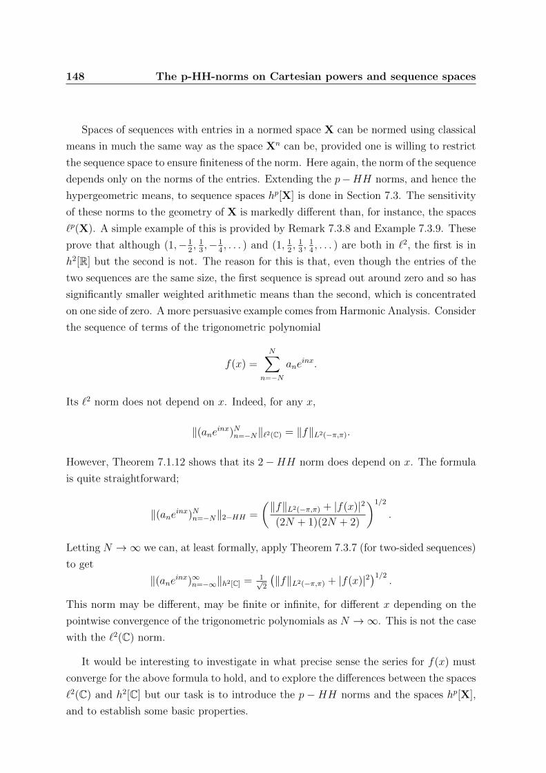
148 The p-HH-norms on Cartesian powers and sequence spaces
Spaces of sequences with entries in a normed space X can be normed using classical
means in much the same way as the space Xn can be, provided one is willing to restrict
the sequence space to ensure finiteness of the norm. Here again, the norm of the sequence
depends only on the norms of the entries. Extending the p−HH norms, and hence the
hypergeometric means, to sequence spaces hp[X] is done in Section 7.3. The sensitivity
of these norms to the geometry of X is markedly different than, for instance, the spaces
`p(X). A simple example of this is provided by Remark 7.3.8 and Example 7.3.9. These
prove that although (1,−12, 1
3,−1
4, . . . ) and (1, 1
2, 1
3, 1
4, . . . ) are both in `2, the first is in
h2[R] but the second is not. The reason for this is that, even though the entries of the
two sequences are the same size, the first sequence is spread out around zero and so has
significantly smaller weighted arithmetic means than the second, which is concentrated
on one side of zero. A more persuasive example comes from Harmonic Analysis. Consider
the sequence of terms of the trigonometric polynomial
f(x) =N∑
n=−N
aneinx.
Its `2 norm does not depend on x. Indeed, for any x,
‖(aneinx)Nn=−N‖`2(C) = ‖f‖L2(−π,π).
However, Theorem 7.1.12 shows that its 2−HH norm does depend on x. The formula
is quite straightforward;
‖(aneinx)Nn=−N‖2−HH =
(‖f‖L2(−π,π) + |f(x)|2
(2N + 1)(2N + 2)
)1/2
.
Letting N →∞ we can, at least formally, apply Theorem 7.3.7 (for two-sided sequences)
to get
‖(aneinx)∞n=−∞‖h2[C] = 1√2
(‖f‖L2(−π,π) + |f(x)|2
)1/2.
This norm may be different, may be finite or infinite, for different x depending on the
pointwise convergence of the trigonometric polynomials as N →∞. This is not the case
with the `2(C) norm.
It would be interesting to investigate in what precise sense the series for f(x) must
converge for the above formula to hold, and to explore the differences between the spaces
`2(C) and h2[C] but our task is to introduce the p −HH norms and the spaces hp[X],
and to establish some basic properties.

The p-HH-norms on Cartesian powers and sequence spaces 149
The equivalence of the p-norms and the p-HH-norms on X2 follows from the Hermite-
Hadamard inequality and Theorem 3.3.2. For the case of n > 2, we utilize the n-
dimensional Hermite-Hadamard inequality to get the upper bound for the p-HH-norms
in terms of the p-norms. For the lower bound, the strict analogue of Theorem 3.3.2 fails,
but a substitute is given, which is also sharp.
A brief examination of the smoothness and convexity properties of the p-HH-norms
on Xn follows. In keeping with the methods of Chapter 3, an isometric embedding of
Xn into a Lebesgue-Bochner space is given. This embedding facilitates the proofs of the
geometrical results. A formula for the semi-inner products is also presented and is used
to prove that (Gateaux) smoothness of the space Xn is inherited from X.
Extending the p-HH-norm from Xn to a suitable space of sequences reveals funda-
mental differences between the p-HH-norms and the p-norms. Although the resulting
sequence spaces all lie between `1(X) and `∞(X), it seems that the resemblance to `p(X)
ends there. Examples are given, in the case X = R, to show that the 2-HH-norm ex-
tends to a sequence space that strictly contains `1, that these sequence spaces need not
be lattices; they need not be complete spaces; and they need not even be closed under
a permutation of the terms of the sequence.
7.1 The p-HH-norm on Xn
In Chapter 3, we introduced the p-HH-norms on the Cartesian square of a normed space
(X, ‖ · ‖). The extension of these norms to Xn is presented in this section, as well
as their equivalence to the p-norms. Similarly to the case of n = 2, the consequences
of this equivalence include the completeness and the reflexivity of the p-HH-norms in
Xn, provided that X is complete and reflexive, respectively. We also note that the
2-HH-norm in Xn is induced by an inner product, when X is an inner product space.
7.1.1 Extending the p-HH-norms
In Chapter 3, we introduced the p-HH-norms on the Cartesian square of a normed space
(X, ‖ · ‖) as follows
‖x‖p−HH =
(∫ 1
0
‖(1− t)x1 + tx2‖p dt)1/p

150 The p-HH-norms on Cartesian powers and sequence spaces
for all x = (x1, x2) ∈ X2 and 1 ≤ p <∞. In this section we extend the definition of the
p-HH-norm to Xn for n > 2.
In the case of n = 2, we consider the integral mean on a line segment generated by
two vectors. The line segment is essentially the convex combination of the given pair
of vectors. Therefore, in the case of n > 2, the domain of integration is the convex
combination of n vectors, that is, a simplex generated by n vectors.
Definition 7.1.1 (Kikianty and Sinnamon [75]). Let (X, ‖·‖) be a normed space, n ≥ 2
be an integer and 1 ≤ p <∞. Set
En = (u1, . . . , un−1) ∈ (0, 1)n−1 : u1 + · · ·+ un−1 < 1.
When (u1, . . . , un−1) ∈ En set un = 1 − u1 − · · · − un−1 and du′ = dun−1 . . . du1. For
x = (x1, . . . , xn) ∈ Xn,
‖x‖p−HH =
(1
|En|
∫En
‖u1x1 + · · ·+ unxn‖p du′)1/p
.
Here |En| =∫En
du′ is the measure of the set En.
Note that when n = 2 this definition agrees with the one given in Chapter 3. When
n = 1 it is convenient to set ‖x‖p−HH = ‖x1‖ for x = (x1) ∈ X1.
Theorem 7.1.2 (Kikianty and Sinnamon [75]). Suppose (X, ‖ · ‖) is a normed space, n
is a positive integer and 1 ≤ p <∞. Then ‖ · ‖p−HH is a norm on Xn.
Proof. The triangle inequality in X shows that
(u1, . . . , un−1) 7→ ‖u1x1 + · · ·+ unxn‖p
defines a continuous function on the closure of En, a compact set of finite measure. It
follows that the integral defining the p-HH-norm is finite. The norm is clearly non-
negative and homogeneous. The triangle inequality follows readily from the triangle
inequality in X and the Minkowski inequality. Now suppose that ‖x‖p−HH = 0. Then,
‖u1x1 + · · ·+ unxn‖p = 0 for almost every (u1, · · · , un−1) ∈ En. By continuity it is iden-
tically zero on En; furthermore on the closure of En. In particular, it vanishes at the
points (1, 0, 0, · · · , 0), (0, 1, 0, · · · , 0), · · · , (0, 0, · · · , 0, 1) and (0, 0, · · · , 0). This shows
that x1 = x2 = · · · = xn = 0 and completes the proof.

The p-HH-norms on Cartesian powers and sequence spaces 151
There is a natural definition of the p-HH-norm when p = ∞ but it does not give a
new norm. Indeed, for x = (x1, . . . , xn) ∈ Xn,
‖x‖∞−HH = sup(u1,...,un−1)∈En
‖u1x1 + · · ·+ unxn‖
= max‖x1‖, . . . , ‖xn‖ = ‖x‖∞.
When X = R and x = (x1, . . . , xn) is a vector of positive real numbers, the p-HH-
norm of x is the pth-hypergeometric mean of (x1, . . . , xn), which is constructed from the
unweighted hypergeometric R-function evaluated at (x1, . . . , xn) (cf. Chapter 1).
The p-HH-norms enjoy a simple relationship with each other and with the p-norms on
Xn. Since the integral defining the p-HH-norm is an average, Holder’s inequality shows
that the p-HH-norm is increasing as a function of p on [1,∞). So for 1 < p ≤ q <∞ we
have for all x ∈ Xn
‖x‖1−HH ≤ ‖x‖p−HH ≤ ‖x‖q−HH ≤ ‖x‖∞ ≤ ‖x‖q ≤ ‖x‖p ≤ ‖x‖1
(cf. Remark 3.2.7). It is interesting to compare this observation with Theorem 7.3.2 in
Section 7.3.
7.1.2 Equivalency of the p-norms and the p-HH-norms
We have proven that the p-norms and the p-HH-norms are equivalent in the Cartesian
square, in Chapter 3. In this subsection, we prove that they are equivalent in the nth
Cartesian power, for any positive integer n. We investigate upper and lower bounds for
this new norm, in terms of the p-norms.
For the upper bound, we apply the unweighted case of the n-dimensional Hermite-
Hadamard inequality. The general case is Theorem 1.2.1 of Chapter 1 (Theorem 5.20
of [100]), but we provide an elementary proof of the special case that we use.
In Theorem 3.3.2, we provide a sharp lower bound for the p-HH-norm in terms of the
p-norm on X2. Moreover, the best constant in this lower bound is the same for every
normed space X. This is not the case when n > 2. Example 7.1.9 shows that when
n > 2 the sharp lower bound for the p-HH-norm in terms of the p-norm on Xn may
genuinely depend on the norm of the underlying space X. As a substitute for the sharp
lower bound obtained when n = 2, we provide a sharp lower bound for the p-HH-norm

152 The p-HH-norms on Cartesian powers and sequence spaces
in terms of the ∞-norm,
‖x‖∞ = max‖x1‖, . . . , ‖xn‖.
In this result the best constant does not depend on the space X.
To work effectively with the p-HH-norms we often need to make calculations involving
integration over the simplex En. To assist with such calculations we offer the following
useful changes of variable.
Lemma 7.1.3 (Kikianty and Sinnamon [75]). Let n be a positive integer and f :
(0, 1)n → R be integrable. For (u1, . . . , un−1) ∈ En, set un = 1 − u1 − · · · − un−1
and du′ = dun−1 . . . du1. If σ is a permutation of 1, 2, . . . , n, then∫En
f(u1, . . . , un) du′ =
∫En
f(uσ(1), . . . , uσ(n)) du′. (7.1)
Proof. Let σ be a permutation of 1, 2, . . . , n and consider the change of variables
wi = uσ(i), for all i ∈ 1, 2, . . . , n.
Then, the Jacobian determinant J of this transformation is 1, when σ is an even per-
mutation; and it is -1 when σ is an odd permutation. Therefore,∫En
f(u1, . . . , un) du′ =
∫En
f(uσ(1), . . . , uσ(n))|J | du′
=
∫En
f(uσ(1), . . . , uσ(n)) du′
which completes the proof.
Lemma 7.1.4 (Kikianty and Sinnamon [75]). Let m ≥ 2 and n ≥ 2 be integers and
f : (0, 1)m+n → R be integrable. For (u1, . . . , un−1) ∈ En, (v1, . . . , vm−1) ∈ Em and
(w1, . . . , wm+n−1) ∈ Em+n, set
un = 1− u1 − · · · − un−1, du′ = dun−1 . . . du1,
vm = 1− v1 − · · · − vm−1, dv′ = dvm−1 . . . dv1,
wm+n = 1− w1 − · · · − wm+n−1, dw′ = dwm+n−1 . . . dw1.

The p-HH-norms on Cartesian powers and sequence spaces 153
Then, ∫Em+n
f(w1, . . . , wm+n) dw′ (7.2)
=
∫ 1
0
∫Em
∫En
f(tv1, . . . , tvm, (1− t)u1, . . . , (1− t)un) du′ dv′tm−1(1− t)n−1 dt,
∫En+1
f(w1, . . . , wn+1) dw′ (7.3)
=
∫ 1
0
∫En
f(t, (1− t)u1, . . . , (1− t)un) du′(1− t)n−1 dt
and ∫Em+1
f(w1, . . . , wm+1) dw′ =
∫ 1
0
∫Em
f(tv1, . . . , tvm, 1− t) dv′tm−1 dt. (7.4)
Proof. We only prove (7.2), as the proofs for (7.3) and (7.4) follows as its particular
cases. We consider the following change of variables
wi =
tvi, when i = 1, . . . ,m;
(1− t)ui−m, when i = m+ 1, . . . ,m+ n− 1.
The Jacobian determinant J of this transformation is
J =
∣∣∣∣ ∂(w1, . . . , wm+n−1)
∂(v1, . . . , vm−1, t, u1, . . . , un−1)
∣∣∣∣
=
∣∣∣∣∣∣∣∣∣∣∣∣∣∣∣∣∣∣∣∣∣∣
t · · · 0 v1 0 · · · 0...
. . ....
......
......
0 · · · t vm−1 0 · · · 0
−t · · · −t vm 0 · · · 0
0 · · · 0 −u1 (1− t) · · · 0...
. . ....
...... · · · ...
0 · · · 0 −un−1 0 · · · (1− t)
∣∣∣∣∣∣∣∣∣∣∣∣∣∣∣∣∣∣∣∣∣∣=
m∑i=1
(−1)m+ivi(−t)tm−2(−1)m−i−1(1− t)n−1

154 The p-HH-norms on Cartesian powers and sequence spaces
=m∑i=1
vitm−1(1− t)n−1
= tm−1(1− t)n−1,
since∑m
i=1 vi = 1. Therefore,∫Em+n
f(w1, . . . , wm+n) dw′
=
∫ 1
0
∫Em
∫En
f(tv1, . . . , tvm, (1− t)u1, . . . , (1− t)un) du′ dv′|J | dt
=
∫ 1
0
∫Em
∫En
f(tv1, . . . , tvm, (1− t)u1, . . . , (1− t)un) du′ dv′tm−1(1− t)n−1 dt,
as required.
Remark 7.1.5. With f ≡ 1 equation (7.3) becomes
|En+1| =∫En+1
dw′ =
∫ 1
0
∫En
du′(1− t)n−1 dt =1
n|En|;
and by induction we find that |En| = 1/(n− 1)!.
With these in hand we can easily prove the following (unweighted) n-dimensional
Hermite-Hadamard inequality.
Theorem 7.1.6 (Kikianty and Sinnamon [75]). Suppose X is a vector space, n ≥ 2 is
an integer and f : X→ R is convex. If x = (x1, . . . , xn) ∈ X, then
f
(x1 + · · ·+ xn
n
)≤ 1
|En|
∫En
f(u1x1 + · · ·+ unxn) du′
≤ f(x1) + · · ·+ f(xn)
n.
Proof. Let Sn denote the collection of all permutations of 1, . . . , n and note that Sn
has n! elements. Let (u1, . . . , un−1) ∈ En and set un = 1− u1 − · · · − un−1. For each i,∑σ∈Sn
uσ(i) = (n− 1)!
because each of u1, . . . , un occurs exactly (n−1)! times in the sum and u1 + · · ·+un = 1.

The p-HH-norms on Cartesian powers and sequence spaces 155
By Lemma 7.1.3,
1
|En|
∫En
f(u1x1 + · · ·+ unxn) du′
=1
n!
∑σ∈Sn
1
|En|
∫En
f(uσ(1)x1 + · · ·+ uσ(n)xn) du′
=1
|En|
∫En
1
n!
∑σ∈Sn
f(uσ(1)x1 + · · ·+ uσ(n)xn) du′. (7.5)
Since f is convex and uσ(1) + · · ·+ uσ(n) = 1 for all σ ∈ Sn, the Jensen inequality yields
1
n!
∑σ∈Sn
f(uσ(1)x1 + · · ·+ uσ(n)xn)
≤ 1
n!
∑σ∈Sn
(uσ(1)f(x1) + · · ·+ uσ(n)f(xn)
)=
(1
n!
∑σ∈Sn
uσ(1)
)f(x1) + · · ·+
(1
n!
∑σ∈Sn
uσ(n)
)f(xn)
=f(x1) + · · ·+ f(xn)
n.
On the other hand, the convexity of f also yields
1
n!
∑σ∈Sn
f(uσ(1)x1 + · · ·+ uσ(n)xn)
≥ f
(1
n!
∑σ∈Sn
(uσ(1)x1 + · · ·+ uσ(n)xn)
)
= f
((1
n!
∑σ∈Sn
uσ(1)
)x1 + · · ·+
(1
n!
∑σ∈Sn
uσ(n)
)xn
)
= f
(x1 + · · ·+ xn
n
).
Using these upper and lower bounds for the integrand in (7.5) completes the proof.
Remark 7.1.7. The results involving integration over simplex in this subsection are
special cases of the results in Chapter 5 of Carlson [18]. In particular, the double
inequality in Theorem 7.1.6 is a special case of the inequality in Exercise 5.2-1 of Carlson
[18, p. 118].

156 The p-HH-norms on Cartesian powers and sequence spaces
The following corollary gives a sharp upper bound for the p-HH-norm in terms of the
p-norm on Xn.
Corollary 7.1.8 (Kikianty and Sinnamon [75]). Let (X, ‖ · ‖) be a normed space, n a
positive integer and 1 ≤ p <∞. For x = (x1, . . . , xn) ∈ Xn,∥∥∥∥x1 + · · ·+ xnn
∥∥∥∥ ≤ ‖x‖p−HH ≤ n−1/p‖x‖p. (7.6)
The inequalities reduce to equality when x1 = · · · = xn.
Proof. If n = 1 the statement holds trivially. If n ≥ 2, note that f(x) = ‖x‖p is a convex
function on X. With this f , the conclusion of the previous theorem easily implies (7.6);
just take the pth roots.
When x = (x, . . . , x) for some x ∈ X,∥∥∥∥x1 + · · ·+ xnn
∥∥∥∥ = ‖x‖,
‖x‖p−HH =
(1
|En|
∫En
‖x‖p du′)1/p
= ‖x‖,
and n−1/p‖x‖p = n−1/p (‖x‖p + · · ·+ ‖x‖p)1/p = ‖x‖
as required.
Obtaining a lower bound for the p-HH-norm in terms of the p-norm is more delicate.
Recall that for any x ∈ X2,
(2p+ 2)−1/p‖x‖p ≤ ‖x‖p−HH .
In view of this result it is natural to ask for the best (greatest) constant c in the inequality
c‖x‖p ≤ ‖x‖p−HH (7.7)
for x ∈ Xn. However, as the next example shows, the constant c may be different for
different spaces X.
Example 7.1.9 (Kikianty and Sinnamon [75]). Let n = 3 and p = 2. If X = R, the
best constant for which (7.7) holds is c = 1/√
12. However, if X = R2∞ then (7.7) fails
with c = 1/√
12.

The p-HH-norms on Cartesian powers and sequence spaces 157
Proof. First take X = R. For x = (x1, x2, x3), a straightforward calculation shows that
‖x‖22−HH = 1
6(x2
1 + x22 + x2
3 + x1x2 + x2x3 + x3x1).
Since ‖x‖22 = x2
1 + x22 + x2
3, we see that
0 ≤ (x1 + x2 + x3)2 = 12‖x‖22−HH − ‖x‖2
2,
which proves (7.7) with c = 1/√
12. Take x = (1,−1, 0) to see that no larger value of c
will do.
Now let X = R2∞, that is, X = R2 with norm ‖(t1, t2)‖ = max|t1|, |t2|. Set
x = (x1, x2, x3), where x1 = (−1, 2), x2 = (−1,−2) and x3 = (2, 0). Calculations show
that
‖x‖22 = 12 and ‖x‖2
2−HH = 437/450.
For (7.7) to hold for this vector x we must have 12c2 ≤ 437/450 so (7.7) fails with
c = 1/√
12.
Rather than continuing to pursue a lower bound involving the p-norm directly, we
turn our attention to the ∞-norm and get a lower bound for the p-HH-norm in which
the same constant is sharp for each normed space X. Since the p-norm and the∞-norm
are equivalent, this approach gives, indirectly, a lower bound for the p-HH-norm in terms
of the p-norm.
Theorem 7.1.10 (Kikianty and Sinnamon [75]). Let (X, ‖·‖) be a normed space, n ≥ 2
and integer and 1 ≤ p <∞. The inequality
‖x‖p−HH ≥ c‖x‖∞ (7.8)
holds for all x ∈ Xn, where
cp = inf1≤s≤2
(n− 1)
∫ 1
0
|1− ts|ptn−2 dt.
The constant c is strictly positive and best possible.
Proof. Let x = (x1, . . . , xn) ∈ Xn. The identity (7.1) implies that the p-HH-norm
is invariant under permutations of x1, . . . , xn so we may permute x1, . . . , xn without
changing either side of the inequality above. Therefore we may suppose without loss of

158 The p-HH-norms on Cartesian powers and sequence spaces
generality that ‖x1‖ = max‖x1‖, . . . , ‖xn‖. Set x = (x2 + · · · + xn)/(n− 1) and note
that ‖x‖ ≤ ‖x1‖.
Let σ be the (n− 1)-cycle (2 . . . n) and apply σ to x1, . . . , xn repeatedly to get
‖(x1, x2, . . . , xn)‖p−HH =1
n− 1(‖(x1, x2, . . . , xn)‖p−HH
+ ‖(x1, x3, . . . , xn, x2)‖p−HH+ · · ·+ ‖(x1, xn, x2 . . . , xn−1)‖p−HH)
≥ ‖(x1, x, . . . , x)‖pp−HH .
The last inequality above is the triangle inequality in the p-HH-norm.
If n ≥ 3, (7.3) implies that
‖(x1, x, . . . , x)‖pp−HH =1
|En|
∫En
‖w1x1 + (1− w1)x‖p dw′
=1
|En|
∫ 1
0
∫En−1
‖tx1 + (1− t)x‖p du′(1− t)n−2 dt
= (n− 1)
∫ 1
0
‖(1− t)x1 + tx‖ptn−2 dt.
It is straightforward to check that this equation also holds when n = 2. Putting
these together and applying the triangle inequality in X shows that
‖(x1, x2, . . . , xn)‖pp−HH ≥ (n− 1)
∫ 1
0
|(1− t)‖x1‖ − t‖x‖|ptn−2 dt
= (n− 1)
∫ 1
0
|1− t(1 + ‖x‖/‖x1‖)|ptn−2 dt‖x1‖p
≥ cp‖x1‖p.
Observe that∫ 1
0|1 − ts|ptn−2 dt is a strictly positive, continuous function of s on [1, 2].
The infimum of such a function is strictly positive so c is strictly positive.
To complete the proof we show that c is the best possible constant in (7.8). If
1 ≤ s ≤ 2 and x 6= 0, set
x = (x, (1− s)x, . . . , (1− s)x) ∈ Xn

The p-HH-norms on Cartesian powers and sequence spaces 159
and note that ‖x‖∞ = ‖x‖. On the other hand, if n ≥ 3 then (7.3) implies
‖x‖pp−HH =1
|En|
∫En
‖w1x+ (1− w1)(1− s)x‖p dw′
=‖x‖p
|En|
∫ 1
0
∫En−1
|t+ (1− t)(1− s)|p du′(1− t)n−2 dt
= (n− 1)‖x‖p∫ 1
0
|1− ts|ptn−2 dt.
It is straightforward to check that this equation also holds when n = 2. It follows that
(7.8) fails for any constant larger than c, so c is best possible.
Corollary 7.1.11 (Kikianty and Sinnamon [75]). Let (X, ‖ · ‖) be a normed space, n a
positive integer and 1 ≤ p < ∞. Then, the p-HH-norm is equivalent to the p-norm on
Xn. If X is a Banach space, then (Xn, ‖ · ‖p−HH) is a Banach space. If X is reflexive,
then (Xn, ‖ · ‖p−HH) is also reflexive.
Proof. The Hermite-Hadamard inequality gives an upper bound for the p-HH-norm in
terms of the the p-norm and the previous theorem gives a lower bound for the p-HH-
norm in terms of the ∞-norm. Since the ∞-norm is equivalent to the p-norm there
is a lower bound for the p-HH-norm in terms of the p-norm and so the two norms are
equivalent.
As stated in Proposition 2.2.2, it is known that if X is complete then (Xn, ‖ · ‖p)is also complete. Since the p-HH-norm is equivalent to the p-norm, (Xn, ‖ · ‖p−HH) is
complete as well.
If X is reflexive then (Xn, ‖ · ‖p) is also reflexive (cf. Chapter 2). The equivalence
of the p-norm and the p-HH-norm implies that (Xn, ‖ · ‖p−HH) is reflexive whenever X
is.
7.1.3 The 2-HH-norm
In this subsection, we point out that if the norm in X is induced by a (real) inner
product then the 2-HH-norm in Xn is also induced by an inner product. For convenience
in expressing the formula for the inner product that induces the 2-HH-norm we define
s(x) = x1 + · · ·+ xn for all x = (x1, . . . , xn) ∈ Xn.

160 The p-HH-norms on Cartesian powers and sequence spaces
Theorem 7.1.12 (Kikianty and Sinnamon [75]). Suppose (X, 〈·, ·〉) is an inner product
space and n ≥ 2 is an integer. Then, Xn is an inner product space with respect to the
inner product
〈x,y〉2−HH =1
n(n+ 1)
(〈x,y〉2 + 〈s(x), s(y)〉
)and for all x ∈ Xn we have
‖x‖22−HH = 〈x,x〉2−HH .
Proof. It is a simple matter to check that the formula for 〈·, ·〉2−HH given above does
define an inner product.
To verify that it induces the 2-HH-norm suppose x = (x1, . . . , xn) ∈ Xn. Then,
‖x‖22−HH =
1
|En|
∫En
|u1x1 + · · ·+ unxn|2 du′
= (n− 1)!
∫En
〈u1x1 + · · ·+ unxn, u1x1 + · · ·+ unxn〉 du′
=n∑j=1
n∑k=1
(n− 1)!
∫En
ujuk du′〈xj, xk〉 and
〈x,x〉2−HH =1
n(n+ 1)
(〈x,x〉2 + 〈s(x), s(x)〉
)=
n∑j=1
n∑k=1
δj k + 1
n(n+ 1)〈xj, xk〉
where δj k is 1 when j = k and 0 otherwise.
It remains to show that
(n+ 1)!
∫En
ujuk du′ = δj k + 1 (7.9)
for all j, k. By (7.1) it is enough to show that
(n+ 1)!
∫En
u1u2 du′ = 1 and (n+ 1)!
∫En
u21 du
′ = 2.
When n = 3, we have
4!
∫ 1
0
∫ 1−s
0
ts dtds = 1 and 4!
∫ 1
0
∫ 1−s
0
t2 dtds = 2.

The p-HH-norms on Cartesian powers and sequence spaces 161
When n > 3, we employ (7.2), as follows
(n+ 1)!
∫En
u1u2 du′
= (n+ 1)!
∫ 1
0
∫E3
∫En−3
t2s1s2t2(1− t)n−4 dv′ds1ds2dt
=(n+ 1)!
(n− 4)!
∫ 1
0
t4(1− t)n−4dt
∫ 1
0
∫ 1−s2
0
s1s2 ds1ds2 = 1
and
(n+ 1)!
∫En
u21 du
′ = (n+ 1)!
∫ 1
0
∫E2
∫En−2
t2s2t(1− t)n−3 dv′dsdt
=(n+ 1)!
(n− 3)!
∫ 1
0
t3(1− t)n−3dt
∫ 1
0
s2ds = 2.
This completes the proof.
Remark 7.1.13. The identity (7.9) is a special case of identity (4.4-8) of Carlson [18].
Carlson [18, p. 66] stated that for any n-tuples b = (b1, . . . , bn) and m = (m1, . . . ,mn),
we have ∫En
um11 . . . umk
k dµb(u) =B(b+m)
B(b),
where dµb(u) = 1B(b)
ub1−11 . . . u
bk−1−1k−1 (1− u1 − · · · − uk−1)bk−1du′ and B is the usual Beta
function. By choosing b = (1, . . . , 1) and m to be the vector with all elements of zero
values except for the the jth and kth elements having the value 1, we obtain identity
(7.9).
7.2 Convexity and smoothness
Although the p-HH-norm on Xn is equivalent to the p-norm, it is not identical. Geomet-
rical properties such as convexity and smoothness are not preserved under equivalence
of norms.
In this section we investigate the extent to which geometrical properties of X are
inherited by Xn when it is given the p-HH-norm. In addition, we give simple formulas
for the semi-inner products on (Xn, ‖ · ‖p−HH) in terms of the semi-inner products on X.

162 The p-HH-norms on Cartesian powers and sequence spaces
7.2.1 Strict convexity and uniform convexity
Let (X, ‖ · ‖) be a normed space, n ≥ 2 an integer and 1 ≤ p <∞. Recall that
En = (u1, . . . , xn−1) ∈ (0, 1)n−1 : u1 + · · ·+ un−1 < 1,
du′ = dun−1 . . . du1 and un = 1− u1 − · · · − un−1.
The Lebesgue-Bochner space Lp(En,X) is the vector space of all f : En → X such
that the function
(u1, . . . , un−1) 7→ ‖f(u1, . . . , un−1)‖p
is integrable on En. The norm is given by
‖f‖Lp(En,X) =
(1
|En|
∫En
‖f(u1, . . . , un−1)‖p du′)1/p
and, as usual, functions that agree almost everywhere are taken to be equal. This is a
special case of the Bochner function spaces as stated in Chapter 2. For properties of
the Lebesgue-Bochner spaces, we refer to III.3 of Dunford and Schwartz [48] and for
applications to the geometry of Banach spaces, we refer to Lemma 2.3.4 and the paper
by Randrianantoanina and Saab [103].
For each x = (x1, . . . , xn) ∈ Xn we define the function f : En → X by fx(u1, . . . , un−1) =
u1x1 + · · ·+ unxn. Evidently, the map x 7→ fx is an isometry from (Xn, ‖ · ‖p−HH) into
Lp(En,X).
Using this embedding we show that both types of convexity are preserved as we pass
from X to (Xn, ‖ · ‖p−HH), although we must exclude the case p = 1.
Theorem 7.2.1 (Kikianty and Sinnamon [75]). Let (X, ‖ · ‖) be a normed space, n ≥ 2
an integer and 1 < p < ∞. If X is uniformly convex, then so is (Xn, ‖ · ‖p−HH). If X
is strictly convex, then so is (Xn, ‖ · ‖p−HH).
Proof. Suppose first that X is uniformly convex. Then, Lp(En,X) is also uniformly
convex. It is clear from the definition that any subspace of a uniformly convex space is
also uniformly convex. The above embedding shows that (Xn, ‖ · ‖p−HH) is isometrically
isomorphic to a subspace of Lp(En,X). Therefore (Xn, ‖ · ‖p−HH) is uniformly convex.
The uniform convexity of R is trivial; and it follows that Lp(En,R) is uniformly
convex and hence strictly convex (cf. Theorem 5.2.6 of Megginson [85]).

The p-HH-norms on Cartesian powers and sequence spaces 163
Now suppose that X is strictly convex. The strict convexity of Lp(En,R) and The-
orem 6 of Day [29] together imply that Lp(En,X) is strictly convex. The definition of
strict convexity shows that any subspace of a strictly convex space is strictly convex.
Since (Xn, ‖ · ‖p−HH) is isometrically isomorphic to a subspace of Lp(En,X), it is also
strictly convex.
7.2.2 Smoothness
For Frechet smoothness we exclude the case p = 1 and also require that X be complete.
Theorem 7.2.2 (Kikianty and Sinnamon [75]). Let (X, ‖ · ‖) be a Banach space, n ≥ 2
an integer and 1 < p <∞. If X is Frechet smooth, then so is (Xn, ‖ · ‖p−HH).
Proof. The norm in the Banach space X is Frechet differentiable away from zero so,
according to Theorem 2.5 of Leonard and Sundaresan [79], the norm in Lp(En,X) is
also Frechet differentiable away from zero. In particular, the norm in Lp(En,X) is
Frechet differentiable at each nonzero point of the isometric image of (Xn, ‖ · ‖p−HH) in
Lp(En,X). It follows that (Xn, ‖ · ‖p−HH) is Frechet smooth.
The next result gives formulas for the one-sided derivatives for the p-HH-norm. In a
slight abuse of notation we let
u · x = u1x1 + · · ·+ unxn
where x = (x1, . . . , xn) ∈ Xn and (u1, . . . , un−1) ∈ En, with un = 1− u1 − · · · − un−1 as
usual.
Theorem 7.2.3 (Kikianty and Sinnamon [75]). Let (X, ‖ · ‖) be a normed space, n ≥ 2
an integer and 1 ≤ p <∞. For any x,y ∈ Xn with y 6= 0,
(∇+‖ · ‖p−HH(y))(x) = ‖y‖1−pp−HH
1
|En|
∫En
‖u · y‖p−1(∇+‖ · ‖(u · y))(u · x) du′.
and
〈x,y〉p−HH,s = ‖y‖2−pp−HH
1
|En|
∫En
‖u · y‖p−2〈u · x,u · y〉s du′.
Corresponding formulas hold for the left-hand derivative and the inferior semi-inner
product.

164 The p-HH-norms on Cartesian powers and sequence spaces
Proof. First, observe that if y 6= 0 then the set
(u1, . . . , un−1) ∈ En : u · y = 0
is a section of an affine set of dimension n − 2 and is therefore of measure zero in the
(n− 1)-dimensional set En. This ensures that the expressions ‖u · y‖p−1 and ‖u · y‖p−2
appearing above are well-defined and finite almost everywhere.
Fix x,y ∈ Xn with y 6= 0 and define
ft = ft(u1, . . . , un−1) = ‖u · (y + tx)‖
for all t ∈ (0, 1) and for all (u1, . . . , un−1) ∈ En satisfying u · y 6= 0. The triangle
inequality shows that |ft| ≤ ‖y‖1 + ‖x‖1 for all t and that
1t(ft − f0) ≤ ‖u · x‖ ≤ ‖x‖1 ≤ ‖y‖1 + ‖x‖1.
By the mean value theorem,
|1t(fpt − f
p0 )| ≤ p(‖y‖1 + ‖x‖1)p−1|1
t(ft − f0)| ≤ p(‖y‖1 + ‖x‖1)p.
Thus, 1t(fpt − f
p0 ) is dominated by a constant independent of t and (u1, . . . , un−1).
For almost every (u1, . . . , un−1) ∈ En, f0 = ‖u · y‖ 6= 0 so the chain rule implies
limt→0+
1t(fpt − f
p0 ) = pfp−1
0 (∇+‖ · ‖(u · y))(u · x)
and by Lebesgue’s dominated convergence theorem,
limt→0+
1
t
(∫En
fpt du′ −∫En
fp0 du′)
=
∫En
pfp−10 (∇+‖ · ‖(u · y))(u · x) du′.
Applying the chain rule again gives
limt→0+
1t(‖y + tx‖p−HH − ‖y‖p−HH) = ‖y‖1−p
p−HH
∫En
‖u · y‖p−1(∇+‖ · ‖(u · y))(u · x) du′,
the first formula of the theorem.

The p-HH-norms on Cartesian powers and sequence spaces 165
The second formula follows from the first by applying (2.2). With obvious minor
modifications the proof will apply to the left-hand derivative and the inferior semi-inner
product.
These formulas imply that if the superior and inferior semi-inner products of X agree,
then the superior and inferior semi-inner products of (Xn, ‖ · ‖p−HH) agree, giving the
following corollary.
Corollary 7.2.4 (Kikianty and Sinnamon [75]). Let (X, ‖ · ‖) be a normed space, n ≥ 2
an integer and 1 ≤ p <∞. If X is smooth, then so is (Xn, ‖ · ‖p−HH).
Proof. Since X is smooth, 〈x, y〉s = 〈x, y〉i for all x, y ∈ X. It follows that for all
x,y ∈ Xn with y 6= 0 and for almost all (u1, . . . , un−1) ∈ En,
‖u · y‖2−p〈u · x,u · y〉s = ‖u · y‖2−p〈u · x,u · y〉i.
Theorem 7.2.3 implies that 〈x,y〉p−HH,s = 〈x,y〉p−HH,i for all y 6= 0. It also holds when
y = 0, from the definition of the semi-inner products. Equality of these two semi-inner
products for the p−HH norm implies that (Xn, ‖ · ‖p−HH) is smooth.
7.3 The hp spaces
In this section (cf. Kikianty and Sinnamon [75]), we introduce a space of sequences
of elements of the normed space X. The norm in this sequence space will be based
on the p-HH-norm in Xn. To do this we first renormalize the p-HH-norms so that the
embedding (x1, . . . , xn) 7→ (x1, . . . , xn, 0) of Xn into Xn+1 is an isometry. For 1 ≤ p <∞and n ≥ 2 we define the space hpn = hpn[X] to be Xn with norm
‖(x1, . . . , xn)‖hpn =
(Γ(p+ n)
Γ(p+ 1)Γ(n)
)1/p
‖(x1, . . . , xn)‖p−HH .
For convenience we let hp1[X] = X, with identical norms.
Define
hp = hp[X] =
(x1, x2, . . . ) : limN→∞
supn>m≥N
‖(xm+1, . . . , xn)‖hpn−m= 0

166 The p-HH-norms on Cartesian powers and sequence spaces
and, for (x1, x2, . . . ) ∈ hp, define
‖(x1, x2, . . . )‖hp = limn→∞
‖(x1, x2, . . . , xn)‖hpn . (7.10)
Some work is required before we can show that hp is a normed space.
Theorem 7.3.1 (Kikianty and Sinnamon [75]). The embedding (x1, . . . , xn) 7→ (x1, . . . , xn, 0)
of hpn into hpn+1 is an isometry for n ≥ 1.
Proof. If n = 1 and x1 ∈ X we have
‖(x1, 0)‖php2
=Γ(p+ 2)
Γ(p+ 1)
∫E2
‖w1x1 + (1− w1)0‖p dw′
= ‖x1‖p(p+ 1)
∫ 1
0
wp1 dw1 = ‖x1‖p = ‖x1‖php1 .
Suppose n > 1 and x1, . . . xn ∈ X. Applying (7.4) with m replaced by n yields
‖(x1, . . . , xn, 0)‖phpn+1
=Γ(p+ n+ 1)
Γ(p+ 1)
∫En+1
‖w1x1 + · · ·+ wnxn + wn+10‖p dw′
=Γ(p+ n+ 1)
Γ(p+ 1)
∫ 1
0
∫En
‖tv1x1 + · · ·+ tvnxn‖p dv′tn−1 dt
=Γ(p+ n+ 1)
Γ(p+ 1)
∫ 1
0
tp+n−1 dt
∫En
‖v1x1 + · · ·+ vnxn‖p dv′
=Γ(p+ n+ 1)
Γ(p+ n)
1
p+ n‖(x1, . . . , xn)‖p
hpn
= ‖(x1, . . . , xn)‖phpn.
This completes the proof.
The change of variable (7.1) shows that the norm in hpn is invariant under permuta-
tions of x1, . . . , xn. This observation, together with the embedding lemma just given,
enables us to show that the limit in (7.10) exists for every (x1, x2, . . . ) ∈ hp: It is enough
to show that the sequence ‖(x1, . . . , xn)‖hpn is Cauchy. If m < n, then
‖(x1, . . . , xn)‖hpn ≤ ‖(x1, . . . , xm, 0 . . . , 0)‖hpn + ‖(0, . . . , 0, xm+1, . . . , xn)‖hpn= ‖(x1, . . . , xm)‖hpm + ‖(xm+1, . . . , xn)‖hpn−m
so
‖(x1, . . . , xn)‖hpn − ‖(x1, . . . , xm)‖hpm ≤ ‖(xm+1, . . . , xn)‖hpn−m.

The p-HH-norms on Cartesian powers and sequence spaces 167
The definition of hp shows that the last term goes to zero as m and n go to infinity.
The next theorem shows that the hp spaces are normed spaces.
Theorem 7.3.2 (Kikianty and Sinnamon [75]). If X is a normed space, then hp = hp[X]
is a normed space. Moreover, if 1 ≤ p ≤ q <∞ then
`1(X) ⊂ hq[X] ⊂ hp[X] ⊂ `∞(X)
with continuous inclusions.
Proof. It is easy to verify that hp is a vector space of sequences of elements of X and
that (7.10) defines a non-negative function that is positive homogeneous and satisfies
the triangle inequality. Theorem 7.1.10 may be used to show that the limit in (7.10) is
zero only when (x1, x2, . . . ) = (0, 0, . . . ) but first we need an estimate of the constant c
for n ≥ 2. Set
ϕ(s) = (n− 1)
∫ 1
0
|1− ts|tn−2 dt
and split the integral at t = 1/s to calculate
ϕ(s) = s− 1− s
n
(1− 2
sn
)and ϕ′(s) =
(1− 1
n
)(1− 2
sn
).
Since ϕ is decreasing on [1, 21/n] and increasing on [21/n, 2] its infimum is ϕ(21/n) =
21/n − 1.
By Holder’s inequality,
c = inf1≤s≤2
((n− 1)
∫ 1
0
|1− ts|ptn−2 dt
)1/p
≥ inf1≤s≤2
(n− 1)
∫ 1
0
|1− ts|tn−2 dt = 21/n − 1.
By Theorem 7.1.10 and the definition of the norm in hpn
‖(x1, . . . , xn)‖hpn ≥ (21/n − 1)
(Γ(p+ n)
Γ(p+ 1)Γ(n)
)1/p
max‖x1‖, . . . , ‖xn‖.
The limit as n→∞ of max‖x1‖, . . . , ‖xn‖ is ‖(x1, x2, . . . )‖`∞(X); and Stirling’s formula
shows that
limn→∞
(21/n − 1)
(Γ(p+ n)
Γ(p+ 1)Γ(n)
)1/p
=log 2
Γ(p+ 1)1/p.

168 The p-HH-norms on Cartesian powers and sequence spaces
Thus,
‖(x1, x2 . . . )‖hp ≥ (log 2)Γ(p+ 1)−1/p‖(x1, x2, . . . )‖`∞(X).
This finishes the proof that (7.10) defines a norm by showing that only the zero vector
in hp can have zero norm. It also proves that hp is contained in `∞(X) with continuous
inclusion.
Next we show that hp contains `1(X). If 0 ≤ m < n then the permutation invariance
of the hpn norm, together with the isometry of the embeddings hpn → hpn+1 yields
‖(xm+1, . . . , xn)‖hpn−m≤ ‖(xm+1, 0, . . . , 0)‖hpn−m
+ · · ·+ ‖(0, . . . , 0, xn)‖hpn−m
= ‖xm+1‖+ · · ·+ ‖xn‖.
If (x1, x2, . . . ) ∈ `1(X) then this sum tends to zero as m,n → ∞ so, by definition,
(x1, x2, . . . ) ∈ hp. Moreover, taking m = 0 above gives,
‖(x1, x2, . . . )‖hp = limn→∞
‖(x1, . . . , xn)‖hpn≤ lim
n→∞(‖x1‖+ · · ·+ ‖xn‖) = ‖(x1, x2, . . . )‖`1(X).
This shows that the inclusion is continuous.
As mentioned previously, the p-HH-norm is defined as an integral average so Holder’s
inequality shows that for any x ∈ Xn,
‖x‖p−HH ≤ ‖x‖q−HH
when p ≤ q. In terms of the hp and hq norms this is,
‖x‖hpn ≤Γ(q + 1)1/q
Γ(p+ 1)1/p
(Γ(p+ n)
Γ(n)
)1/p(Γ(n)
Γ(q + n)
)1/p
‖x‖hqn . (7.11)
By Stirling’s formula,
limn→∞
(Γ(p+ n)
Γ(n)
)1/p(Γ(n)
Γ(q + n)
)1/p
= 1.
Therefore, the constant
Cp,q = supn
Γ(q + 1)1/q
Γ(p+ 1)1/p
(Γ(p+ n)
Γ(n)
)1/p(Γ(n)
Γ(q + n)
)1/p
,

The p-HH-norms on Cartesian powers and sequence spaces 169
is finite, independent of n and satisfies
‖x‖hpn ≤ Cp,q‖x‖hqn .
This implies that hq ⊂ hp. In addition, taking the limit in (7.11) yields
‖x‖hp ≤Γ(q + 1)1/q
Γ(p+ 1)1/p‖x‖hq
for all x ∈ hq, showing that the inclusion is continuous.
Remark 7.3.3. Since hp contains `1 it contains all sequences that are eventually zero.
Theorem 7.3.1 shows that for these sequences the norm in hp reduces to the norm in hpn
for some n. That is,
‖(x1, x2, . . . , xn, 0, 0, . . . )‖hp = ‖(x1, x2, . . . , xn)‖hpn .
Remark 7.3.4. It is important to distinguish between the spaces hp[X] and hp[R](X).
The latter provides a norm on the space
hp[R](X) = (x1, x2, . . . ) : (‖x1‖, ‖x2‖, . . . ) ∈ hp[R]
given by
‖(x1, x2, . . . )‖hp[R](X) = ‖(‖x1‖, ‖x2‖, . . . )‖hp[R].
Even in the case X = R the spaces hp[X] and hp[R](X) are not the same, although in
this special case the two norms do coincide on vectors with non-negative entries.
The next example shows that the spaces hp[X] need not be complete, even if the
underlying space X is complete. In the example, X = R but, since every non-trivial
normed space contains an isometric copy of R, the example is easily adapted to any X.
Example 7.3.5 (Kikianty and Sinnamon [75]). The normed space h2[R] is not complete.
Proof. Consider the sequence (a, . . . , a, b, . . . , b, 0, 0, . . . ) in which the first m entries
equal a ∈ R, the next n entries equal b ∈ R and the rest of the entries are zero. If
m,n ≥ 2 we use (7.2) to get
‖(a, . . . , a, b, . . . , b, 0, 0, . . . )‖2h2
= ‖(a, . . . , a, b, . . . , b)‖2h2m+n

170 The p-HH-norms on Cartesian powers and sequence spaces
=(m+ n+ 1)!
2
∫Em+n
|(w1 + · · ·+ wm)a+ (wm+1 + · · ·+ wm+n)b|2 dw′
=(m+ n+ 1)!
2
∫ 1
0
∫Em
∫En
(ta+ (1− t)b)2 dv′ du′ tm−1(1− t)n−1 dt
=(m+ n+ 1)!
2(m− 1)!(n− 1)!
∫ 1
0
(ta+ (1− t)b)2 tm−1(1− t)n−1 dt
= 12m(m+ 1)a2 +mnab+ 1
2n(n+ 1)b2.
Similar arguments using (7.3), (7.4) show that the conclusion remains valid when m,n ≥0.
In particular, if ξn = ( 1n, . . . 1
n, 0, 0, . . . ) is chosen to have exactly n non-zero entries
then ‖ξn‖2h2 = (n + 1)/(2n). Since ‖ξn‖h2 → 1/
√2 as n → ∞ the sequence ξn does
not converge to 0 in h2. However, ξn does converge to 0 in `∞ so ξn cannot have a
limit at all in the smaller space h2.
On the other hand, the above calculation shows that
‖ξm+n − ξm‖2h2 = 1
2m(m+ 1)
(1
m+ n− 1
m
)2
+ mn
(1
m+ n− 1
m
)(1
m+ n
)+ 1
2n(n+ 1)
(1
m+ n
)2
=n
2m(m+ n)≤ 1
2m.
Since ‖ξm+n − ξm‖h2 → 0 uniformly in n as m → ∞ the sequence ξn is a Cauchy
sequence in h2. As we have seen, ξn does not converge in h2. Thus h2 is not complete.
Remark 7.3.6. The formula,
‖(a, . . . , a, b, . . . , b, 0, 0, . . . )‖2h2 = 1
2m(m+ 1)a2 +mnab+ 1
2n(n+ 1)b2
given above, shows that h2[R] does not have the lattice property since replacing a by
−a may affect the norm in h2[R].
When X is an inner product space, h2[X] is too. Also, there is a simple for-
mula relating their inner products. Recall that s : Xn → X was defined earlier by

The p-HH-norms on Cartesian powers and sequence spaces 171
s(x1, . . . , xn) = x1 + · · · + xn. By identifying (x1, . . . , xn) ∈ Xn with the sequence
(x1, . . . , xn, 0, 0, . . . ) we can extend this definition to
s(x1, x2, . . . ) = x1 + x2 + . . .
for all sequences (x1, x2, . . . ) that are eventually zero.
Theorem 7.3.7 (Kikianty and Sinnamon [75]). If X is a (real) inner product space,
then h2 = h2[X] ⊂ `2(X), the operator s extends uniquely to a bounded linear operator
on h2; and h2 is an inner product space satisfying
〈x,y〉h2 =1
2
(〈x,y〉2 + 〈s(x), s(y)〉
)(7.12)
for all x,y ∈ h2.
Proof. By Theorem 7.1.12, (Xn, ‖ · ‖2−HH) is an inner product space and consequently
so is h2n. Moreover, for all x,y ∈ Xn,
〈x,y〉h2n = 12n(n+ 1)〈x,y〉2−HH =
1
2
(〈x,y〉2 + 〈s(x), s(y)〉
).
Taking y = x in this equation implies
‖x‖2 ≤√
2‖x‖h2n (7.13)
and
‖s(x)‖ ≤√
2‖x‖h2n . (7.14)
For x = (x1, x2, . . . ) ∈ h2 set x(n) = (x1, . . . , xn) ∈ Xn. Inequality (7.13) shows that
‖x‖2 = limn→∞
‖x(n)‖2 ≤√
2 limn→∞
‖x(n)‖h2 =√
2‖x‖h2 .
Thus, x ∈ `2(X) and we have h2 ⊂ `2(X). Inequality (7.14) shows that if x1, x2, . . . is
eventually zero, then
‖s(x)‖ = limn→∞
‖s(x(n))‖ ≤√
2 limn→∞
‖x(n)‖h2 =√
2‖x‖h2 .

172 The p-HH-norms on Cartesian powers and sequence spaces
The definition of h2 implies that x(n) → x in h2 so the space of sequences that are
eventually zero is dense in h2. We have shown that the linear operator s is densely
defined and bounded on h2. It therefore extends uniquely to a bounded linear map on
h2, which we also denote by s.
The map
(x,y) 7→ 1
2
(〈x,y〉2 + 〈s(x), s(y)〉
)is an inner product on h2 and the norm it defines,
x 7→ 12
(‖x‖2
2 + ‖s(x)‖2),
agrees with the norm in h2 on a dense subset. Therefore, h2 is an inner product space
and (7.12) holds for all x,y ∈ h2.
Remark 7.3.8. If X is an inner product space then `2(X) 6= h2[X]. To see this, fix
a unit vector x ∈ X. The sequence (x, x/2, x/3, . . . ) is in `2(X) because the series
12 + (1/2)2 + (1/3)2 + . . . converges. However, for any m,
supm<n‖(x/(m+ 1), . . . , x/n)‖2
h2n−m= sup
m<n
1
2
n∑k=m+1
1
k2+
(n∑
k=m+1
1
k
)2 =∞.
By definition, (x, x/2, x/3, . . . ) /∈ h2.
In the next example we construct an element of h2 that is not in `1, showing that
the inclusion `1 ⊂ h2 is strict.
Example 7.3.9 (Kikianty and Sinnamon [75]). When X = R, h2 6⊂ `1.
Proof. The sequence (1,−12, 1
3,−1
4, . . . ) is not in `1. However, if m < n then
∥∥∥∥((−1)m
m+ 1, . . . ,
(−1)n−1
n
)∥∥∥∥h2n−m
=1
2
n∑j=m+1
1
j2+
∣∣∣∣∣n∑
j=m+1
(−1)j−1
j
∣∣∣∣∣2
can be made arbitrarily small by taking m sufficiently large. This shows that the se-
quence (1,−12, 1
3,−1
4, . . . ) is in h2.
The permutation invariance of the p-norms carries over from finite dimensional spaces
to sequence spaces. In contrast, the permutation invariance of the norm on hpn may be

The p-HH-norms on Cartesian powers and sequence spaces 173
lost in the transition to hp. We have seen that (1,−12, 1
3,−1
4, . . . ) ∈ h2 but it is a simple
matter to rearrange the terms of the conditionally convergent series 1− 12
+ 13− 1
4+ . . .
so that its partial sums are unbounded. The resulting sequence is not in h2.

174
Chapter 8
Conclusion and future work
In this chapter, we summarize the work of this dissertation, recall the main achievements,
discuss some open problems that are yet to be addressed and suggest the future research
to be undertaken.
8.1 Summary
The p-HH-norm (1 ≤ p <∞) is defined on the Cartesian square X2 of a normed space
(X, ‖ · ‖), by the following
‖(x, y)‖p−HH :=
(∫ 1
0
‖(1− t)x+ ty‖pdt) 1
p
, (x, y) ∈ X2.
It is connected with the p-norms by the Hermite-Hadamard inequality∥∥∥∥x+ y
2
∥∥∥∥ ≤ ‖(x, y)‖p−HH ≤1
21p
‖(x, y)‖p, (x, y) ∈ X2. (8.1)
Together with the following inequality
1
(2p+ 2)1p
‖(x, y)‖p ≤ ‖(x, y)‖p−HH , (x, y) ∈ X2,
the Hermite-Hadamard inequality (8.1) shows that the p-HH-norms and the p-norms are
equivalent in X2. However, they are geometrically different, as pointed out in Example
3.2.4 of Chapter 3.
175

176 Conclusion and future work
As a consequence of the Holder inequality, the relationship amongst the p-norms and
the p-HH-norms is highlighted in the following inequalities, for 1 ≤ p ≤ q <∞,
‖(x, y)‖p−HH ≤ ‖(x, y)‖q−HH ≤ ‖(x, y)‖∞ ≤ ‖(x, y)‖q ≤ ‖(x, y)‖p,
for all (x, y) ∈ X2. In conjunction with the Hermite-Hadamard inequality (8.1), some
quantitative comparisons between the p-HH-norm and the p-norm (for a fixed 1 ≤p < ∞) are derived by some inequalities of Ostrowski type. These inequalities bound
the counterpart of the second Hermite-Hadamard inequality, that is, the difference1
21p‖(x, y)‖p − ‖(x, y)‖p−HH . In the same spirit, the comparisons amongst the p-HH-
norms are derived by some inequalities of Gruss type. These inequalities bound the
Cebysev difference ‖(x, y)‖p+qp+q−HH − ‖(x, y)‖pp−HH‖(x, y)‖qq−HH . Some of these inequali-
ties are proven to be sharp.
When X = R, the p-HH-norm resembles a familiar concept, that is, the pth order
generalized logarithmic mean of two positive numbers. Although the generalized loga-
rithmic mean has been studied since its introduction in 1975 by Stolarsky [113], it is
investigated from a different point of view in this dissertation, that is, by the norm
structure given by it.
The properties of the p-HH-norms can be summarized as follows:
1. They preserve the completeness and reflexivity of X;
2. They preserve the smoothness of X (note that in contrast to the 1-norm, the 1-
HH-norm preserves the smoothness of X);
3. Excluding the case of p = 1, they preserve the Frechet smoothness, strict convexity
and uniform convexity of X.
The 2-HH-norm, in particular, is a Hilbert norm in X2, provided that X is an inner
product space. Using this norm, some notions of orthogonality in normed spaces are
defined:
1. HH-P-orthogonality: x ⊥HH−P y if and only if∫ 1
0
‖(1− t)x+ ty‖2 dt =1
3(‖x‖2 + ‖y‖2);
Conclusion and future work 177
2. HH-I-orthogonality: x ⊥HH−I y if and only if∫ 1
0
‖(1− t)x+ ty‖2dt =
∫ 1
0
‖(1− t)x− ty‖2dt;
3. HH-C-orthogonality: x ⊥HH−C y if and only if
m∑i=1
αi
∫ 1
0
‖(1− t)βix+ tγiy‖2 dt = 0,
where αi, βi, γi ∈ R,∑m
i=1 αiβ2i =
∑mi=1 αiγ
2i = 0 and
∑mi=1 αiβiγi = 1.
They are shown to be closely related to the Pythagorean, Isosceles and Carlsson’s or-
thogonalities, respectively, by the following relation:
“If x, y ∈ X such that (1− t)x ⊥ ty (P ) for almost every t ∈ (0, 1), then x ⊥HH−P y.”
Similar statements hold for I-orthogonality and HH-I-orthogonality, as well as C-orthogonality
and HH-C-orthogonality. The homogeneity, or the additivity (to the left), of these or-
thogonalities characterize inner product spaces. The uniqueness of HH-I-orthogonality
characterizes strictly convex spaces.
The p-HH-norms are then extended to Xn, by the following
‖x‖p−HH =
(1
|En|
∫En
‖u1x1 + · · ·+ unxn‖p du′)1/p
,x = (x1, . . . , xn) ∈ Xn
where |En| =∫En
du′ is the measure of the set
En = (u1, . . . , un−1) ∈ (0, 1)n−1 : u1 + · · ·+ un−1 < 1,
(u1, . . . , un−1) ∈ En, un = 1 − u1 − · · · − un−1 and du′ = dun−1 . . . du1. The similar
properties (of the p-HH-norms in X2) hold in this extension.
The p-HH-norms are extended from Xn to the spaces of sequences of elements in X,
that is,
hp = hp[X] =
(x1, x2, . . . ) : limN→∞
supn>m≥N
‖(xm+1, . . . , xn)‖hpn−m= 0
where
‖(x1, . . . , xn)‖hpn =
(Γ(p+ n)
Γ(p+ 1)Γ(n)
)1/p
‖(x1, . . . , xn)‖p−HH .

178 Conclusion and future work
The hp spaces are normed spaces with the following norm
‖(x1, x2, . . . )‖hp = limn→∞
‖(x1, x2, . . . , xn)‖hpn .
The resulting sequence spaces all lie between `1(X) and `∞(X). The space h2[X]
is an inner product space, provided that X is an inner product space. However, the
resemblance to `p(X) ends there. Some examples show that:
1. The 2-HH-norm extends to a sequence space that strictly contains `1;
2. These sequence spaces need not be lattices;
3. They need not be complete spaces;
4. They need not to be closed under a permutation of the terms of the sequence.
8.2 Main achievements
This section covers the main contributions of the work in the dissertation. The contri-
butions include those in Banach space theory and classical analysis, such as the theory
of inequalities and the theory of means.
The main contribution of the thesis is in Banach space theory, that is, the develop-
ment of a new family of norms in the Cartesian power of a normed space. These norms
behave ‘nicely’, in the sense that they preserve some of the metrical and geometrical
properties of the underlying normed spaces. In particular, the 1-HH-norm preserves the
smoothness, in contrast to the 1-norm, which is not a smooth norm, even when the
underlying space is a smooth space. Using a limit of isometric embeddings, the norms
are extended to spaces of bounded sequences that include all summable sequences.
The thesis has also contributed in the study of Banach space geometry. The 2-
HH-norm is employed to define some notions of orthogonality in normed space. The
homogeneity, as well as the additivity (to the left), of these orthogonalities characterizes
inner product space. In particular, the uniqueness of HH-I-orthogonality characterizes
strictly convex space.
In the theory of inequalities, this thesis contributes firstly in the refinement of the
Hermite-Hadamard inequality for functions defined on linear spaces. This refinement

Conclusion and future work 179
generalizes the results by Dragomir [33,34] and proves the sharpness of the inequalities
that have not been addressed in the corresponding work. The results in Chapter 4
also contributes to the development of Ostrowski type inequalities in normed spaces.
Lastly, the results in Chapter 5, gives some new bounds to the Cebysev functional in
the Riemann-Stieltjes integral approximation.
In the theory of means, the study of the p-HH-norms shows that the norms are
related to the hypergeometric means (generalized logarithmic means, when n = 2), but
are not restricted to the positive real numbers. Therefore, they extend the concept of
hypergeometric means to a more general setting of vector space. In extending the p-HH-
norms to the hp spaces, these norms also extend the hypergeometric mean to infinite
sequences, when the underlying space is the field of real numbers.
8.3 Future work
This section discusses some open problems and further research to be undertaken re-
garding the work of this thesis.
There are several open problems yet to be addressed. The matter of the sharpness of
inequalities in Chapter 4 and Chapter 5 can be demonstrated in some particular cases,
but the analytical proofs have not been given. The following are the lists of conjectures
and open problems related to the sharpness of inequalities:
1. Conjectures 4.3.8, 4.4.1 and 4.4.2 of Chapter 4;
2. Open problems 5.2.5, 5.3.5 and 5.4.10 of Chapter 5.
In Chapter 6, we introduce the notions of orthogonality in normed space via the
2-HH-norm and investigate their properties. We are interested in further research on
the HH type orthogonality, in particular, investigating their applications.
In extending the p-HH-norms to Xn, it is natural to consider the analogous inequal-
ities to those described in Chapters 4 and 5. These inequalities will give refinements
and extensions to the multivariate Hermite-Hadamard inequalities and the multivariate
Gruss type inequality.
It is also of interest to investigate the application of the p-HH-norms in interpolation
spaces due to the following relation:

180 Conclusion and future work
`1 ⊂ hq ⊂ hp ⊂ `∞
for 1 ≤ p ≤ q < ∞. We are also interested in investigating the application of the
p-HH-norms in function spaces. A possible application in function spaces is described
in Appendix A.
The hp spaces are also of interest, which requires further development. The notion
of completeness in hp spaces are yet to be investigated. We may employ the ‘standard’
method of completing the space, but there is no guarantee that the resulting space is
the space of sequences.

Conclusion and future work 181

182

Appendix A
Possible applications of the
p-HH-norms
A.1 Lebesgue space
Let 1 ≤ p <∞ and f be an element of Lp[−1, 1]. The usual Lebesgue norm is given by
‖f‖Lp[−1,1] :=
(∫ 1
−1
|f(t)|p dt)1/p
, f ∈ Lp[−1, 1].
Observe that for any f ∈ Lp[−1, 1], we have
‖f‖Lp[−1,1] =
(∫ 1
−1
|f(t)|pdt) 1
p
=
(∫ 0
−1
|f(t)|pdt+
∫ 1
0
|f(t)|pdt) 1
p
=
(∫ 1
0
|f(−t)|pdt+
∫ 1
0
|f(t)|pdt) 1
p
.
Now, let g be the restriction of f on the interval [0, 1] and h be a function such that
h(t) := f(−t) for any t ∈ [0, 1]. Therefore,
‖f‖Lp[−1,1] =
(∫ 1
0
|f(−t)|pdt+
∫ 1
0
|f(t)|pdt) 1
p
=
(∫ 1
0
|h(t)|pdt+
∫ 1
0
|g(t)|pdt) 1
p
=(‖h‖pLp[0,1] + ‖g‖pLp[0,1]
) 1p. (A.1)
183

184 Possible applications of the p-HH-norms
By (A.1), we may identify f as an element of Lp[0, 1] × Lp[0, 1]. Note that the space
Lp[0, 1]× Lp[0, 1] together with the p-norm, is Lp[−1, 1] with the usual Lebesgue norm.
Now, define the following mapping |‖ · ‖|Lp[−1,1] on Lp[−1, 1] by utilizing the p-HH-
norm, as follows
|‖f‖|Lp[−1,1] := ‖(g, h)‖p−HH =
(∫ 1
0
‖(1− t)g + th‖pLp[0,1]dt
) 1p
=
(∫ 1
0
∫ 1
0
|(1− t)g(s) + th(s)|pdsdt) 1
p
=
(∫ 1
0
∫ 1
0
|(1− t)f(s) + tf(−s)|pdsdt) 1
p
.
It can be easily shown that this mapping is also a norm on Lp[−1, 1].
Note that from inequality (3.3) and Theorem 3.3.2, we have the following identity
1
[2(p+ 1)]1p
‖f‖Lp[−1,1] ≤ |‖f‖|Lp[−1,1] ≤1
21p
‖f‖Lp[−1,1], (A.2)
for any f ∈ Lp[−1, 1].
The following example shows that the constants 1
[2(p+1)]1p
and 1
21p
are best possible in
(A.2).
Example A.1.1. Let f ∈ Lp[−1, 1] be an odd function. We have
|‖f‖|Lp[−1,1] =
[∫ 1
0
(∫ 1
0
|(1− t)f(s) + tf(−s)|pds)dt
] 1p
=
[∫ 1
0
(∫ 1
0
|(1− t)f(s)− tf(s)|pds)dt
] 1p
=
[∫ 1
0
(∫ 1
0
|1− 2t|p|f(s)|pds)dt
] 1p
=
(1
p+ 1
) 1p
‖f‖Lp[0,1] =
(1
2(p+ 1)
) 1p
‖f‖Lp[−1,1].
This shows that the constant(
12(p+1)
) 1p
is best possible in the first inequality of (A.2).

Possible applications of the p-HH-norms 185
Let g ∈ Lp[−1, 1] be an even function. We have
|‖g‖|[−1,1] =
[∫ 1
0
(∫ 1
0
|(1− t)g(s) + tg(−s)|pds)dt
] 1p
=
[∫ 1
0
(∫ 1
0
|(1− t)g(s) + tg(s)|pds)dt
] 1p
=
[∫ 1
0
(∫ 1
0
|g(s)|pds)dt
] 1p
= ‖g‖Lp[0,1] =1
21p
‖g‖Lp[−1,1].
This shows that the constant 1
21p
is best possible in the second inequality of (A.2).
A.2 Linear operator
In this section, we extend the idea in Section A.1 to a more general setting.
Proposition A.2.1. Let (X, ‖ · ‖) be a (real) normed space and U : X→ X be a linear
operator. Define
‖x‖[p] := ‖(x, Ux)‖p−HH =
(∫ 1
0
‖(1− t)x+ tUx‖pdt) 1
p
,
for any x ∈ X. Then, ‖ · ‖[p] is a norm on X.
Proof. Let x = 0, then Ux = 0 (by linearity), thus implies that ‖x‖[p] = 0. Conversely,
let ‖x‖[p] = ‖(x, Ux)‖p−HH = 0, then Ux = −x, by the Hermite-Hadamard inequality.
Now, we have 0 = ‖(x,−x)‖p−HH =(
1p+1
) 1p ‖x‖. Therefore x = 0 since
(1p+1
) 1p 6= 0.
For any x ∈ X and α ∈ R, we have
‖αx‖[p] = ‖(αx, U(αx))‖p−HH = ‖(αx, αU(x))‖p−HH

186 Possible applications of the p-HH-norms
by linearity. Therefore,
‖αx‖[p] =
(∫ 1
0
‖(1− t)αx+ tαUx‖pdt) 1
p
= |α|(∫ 1
0
‖(1− t)x+ tUx‖pdt) 1
p
= |α|‖x‖[p].
We also have for any x, y ∈ X
‖x+ y‖[p] = ‖(x+ y, U(x+ y))‖p−HH
=
(∫ 1
0
‖(1− t)(x+ y) + tU(x+ y)‖pdt) 1
p
=
(∫ 1
0
‖(1− t)(x+ y) + t(Ux+ Uy)‖pdt) 1
p
≤(∫ 1
0
‖(1− t)x+ tUx‖pdt) 1
p
+
(∫ 1
0
‖(1− t)y + tUy‖pdt) 1
p
= ‖x‖[p] + ‖y‖[p],
which proves the triangle inequality.
Example A.2.2. Let U : Lp[a, b]→ Lp[a, b], where Uf(t) = f(a+ b− t). Then,
‖f‖[p] :=
(∫ 1
0
‖(1− t)f + tUf‖pLp[a,b]dt
) 1p
=
(∫ 1
0
∫ b
a
|(1− t)f(s) + tf(a+ b− s)|pdsdt) 1
p
.
Particularly, when a = −1 and b = 1, we have
‖f‖[p] =
(∫ 1
0
∫ 1
−1
|(1− t)f(s) + tf(−s)|pdsdt) 1
p
= 21p
(∫ 1
0
∫ 1
0
|(1− t)f(s) + tf(−s)|pdsdt) 1
p
= 21p |‖f‖|Lp[−1,1],
where |‖ · ‖|Lp[−1,1] is the norm defined in Section A.1.


188

Colophon
This thesis was made in LATEX 2ε using the “hepthesis” class.
189

190
References
[1] M. Aigner and G. M. Ziegler, Proofs from The Book, third ed., Springer-Verlag,
Berlin, 2004.
[2] C. D. Aliprantis and O. Burkinshaw, Principles of Real Analysis, North-Holland
Publishing Co., New York, 1981.
[3] J. Alonso and C. Benıtez, Orthogonality in normed linear spaces: a survey. I. Main
properties, Extracta Math. 3 (1988), no. 1, 1–15.
[4] , Orthogonality in normed linear spaces: a survey. II. Relations between
main orthogonalities, Extracta Math. 4 (1989), no. 3, 121–131.
[5] D. Amir, Characterizations of Inner Product Spaces, Operator Theory: Advances
and Applications, vol. 20, Birkhauser Verlag, Basel, 1986.
[6] G. A. Anastassiou, Ostrowski type inequalities, Proc. Amer. Math. Soc. 123 (1995),
no. 12, 3775–3781.
[7] W. Arendt, C. J. K. Batty, M. Hieber, and F. Neubrander, Vector-valued
Laplace Transforms and Cauchy Problems, Monographs in Mathematics, vol. 96,
Birkhauser Verlag, Basel, 2001.
[8] N. S. Barnett, C. Buse, P. Cerone, and S. S. Dragomir, Ostrowski’s inequality for
vector-valued functions and applications, Comput. Math. Appl. 44 (2002), no. 5-6,
559–572.
[9] E. F. Beckenbach, Convex functions, Bull. Amer. Math. Soc. 54 (1948), 439–460.
[10] E. F. Beckenbach and R. Bellman, Inequalities, Springer-Verlag, New York/Berlin,
1961.
[11] G. Birkhoff, Orthogonality in linear metric spaces, Duke Math. J. 1 (1935), no. 2,
169–172.
191

192 References
[12] S. Bochner, Integration von Functionen, deren Werte die Elemente eines Vektor-
raumes sind, Fund. Math. 20 (1933), 262–276.
[13] S. Bochner and A. E. Taylor, Linear functionals on certain spaces of abstractly-
valued functions, Ann. of Math. (2) 39 (1938), no. 4, 913–944.
[14] P. S. Bullen, Handbook of Means and their Inequalities, Mathematics and its Ap-
plications, vol. 560, Kluwer Academic Publishers Group, Dordrecht, 2003, Revised
from the 1988 original [P. S. Bullen, D. S. Mitrinovic and P. M. Vasic, Means and
their Inequalities, Reidel, Dordrecht; MR0947142].
[15] F. Burk, Notes: The Geometric, Logarithmic, and Arithmetic mean inequality,
Amer. Math. Monthly 94 (1987), no. 6, 527–528.
[16] B. C. Carlson, Some inequalities for hypergeometric functions, Proc. Amer. Math.
Soc. 17 (1966), 32–39.
[17] , The logarithmic mean, Amer. Math. Monthly 79 (1972), 615–618.
[18] B. C. Carlson, Special Functions of Applied Mathematics, Academic Press [Har-
court Brace Jovanovich Publishers], New York, 1977.
[19] S. O. Carlsson, Orthogonality in normed linear spaces, Ark. Mat. 4 (1962), 297–318
(1962).
[20] P. Cerone, Three point rules in numerical integration, Nonlinear Anal. 47 (2001),
no. 4, 2341–2352.
[21] , A new Ostrowski type inequality involving integral means over end inter-
vals, Tamkang J. Math. 33 (2002), no. 2, 109–118.
[22] , On relationships between Ostrowski, trapezoidal and Chebychev identities
and inequalities, Soochow J. Math. 28 (2002), no. 3, 311–328.
[23] P. Cerone and S. S. Dragomir, Three point identities and inequalities for n-time
differentiable functions, SUT J. Math. 36 (2000), no. 2, 351–383.
[24] , On some inequalities arising from Montgomery’s identity (Montgomery’s
identity), J. Comput. Anal. Appl. 5 (2003), no. 4, 341–367.
[25] P. Cerone, S. S. Dragomir, and J. Roumeliotis, Some Ostrowski type inequalities for
n-time differentiable mappings and applications, Demonstratio Math. 32 (1999),
no. 4, 697–712.

References 193
[26] J. A. Clarkson, Uniformly convex spaces, Trans. Amer. Math. Soc. 40 (1936),
no. 3, 396–414.
[27] M. M. Day, Some more uniformly convex spaces, Bull. Amer. Math. Soc. 47 (1941),
504–507.
[28] , Some characterizations of inner-product spaces, Trans. Amer. Math. Soc.
62 (1947), 320–337.
[29] , Strict convexity and smoothness of normed spaces, Trans. Amer. Math.
Soc. 78 (1955), 516–528.
[30] S. S. Dragomir, The Ostrowski integral inequality for mappings of bounded varia-
tion, Bull. Austral. Math. Soc. 60 (1999), no. 3, 495–508.
[31] , A generalization of Ostrowski integral inequality for mappings whose
derivatives belong to L1[a, b] and applications in numerical integration, J. Com-
put. Anal. Appl. 3 (2001), no. 4, 343–360.
[32] , A generalization of the Ostrowski integral inequality for mappings whose
derivatives belong to Lp[a, b] and applications in numerical integration, J. Math.
Anal. Appl. 255 (2001), no. 2, 605–626.
[33] , An inequality improving the first Hermite-Hadamard inequality for con-
vex functions defined on linear spaces and applications for semi-inner products,
JIPAM. J. Inequal. Pure Appl. Math. 3 (2002), no. 2, Article 31, 8 pp. (elec-
tronic).
[34] , An inequality improving the second Hermite-Hadamard inequality for con-
vex functions defined on linear spaces and applications for semi-inner products, JI-
PAM. J. Inequal. Pure Appl. Math. 3 (2002), no. 3, Article 35, 8 pp. (electronic).
[35] , An Ostrowski like inequality for convex functions and applications, Rev.
Mat. Complut. 16 (2003), no. 2, 373–382.
[36] , Inequalities of Gruss type for the Stieltjes integral and applications, Kragu-
jevac J. Math. 26 (2004), 89–122.
[37] , Semi-inner Products and Applications, Nova Science Publishers, Inc.,
Hauppauge, NY, 2004.
[38] , Ostrowski type inequalities for functions defined on linear spaces and ap-

194 References
plications for semi-inner products, J. Concr. Appl. Math. 3 (2005), no. 1, 91–103.
[39] , An Ostrowski type inequality for convex functions, Univ. Beograd. Publ.
Elektrotehn. Fak. Ser. Mat. 16 (2005), 12–25.
[40] S. S. Dragomir and I. A. Fedotov, An inequality of Gruss’ type for Riemann-
Stieltjes integral and applications for special means, Tamkang J. Math. 29 (1998),
no. 4, 287–292.
[41] S. S. Dragomir and J. J. Koliha, Two mappings related to semi-inner products and
their applications in geometry of normed linear spaces, Appl. Math. 45 (2000),
no. 5, 337–355.
[42] S. S. Dragomir and C. E. M. Pearce, Selected Topics on Hermite-Hadamard In-
equalities and Applications, RGMIA Monographs, Victoria University, 2000, (ON-
LINE: http://rgmia.vu.edu.au/monographs).
[43] S. S. Dragomir and T. M. Rassias, Generalisations of the Ostrowski Inequality and
Applications, Kluwer Acad. Publ., Dordrecht, 2002.
[44] S. S. Dragomir and S. Wang, A new inequality of Ostrowski’s type in L1 norm
and applications to some special means and to some numerical quadrature rules,
Tamkang J. Math. 28 (1997), no. 3, 239–244.
[45] , Applications of Ostrowski’s inequality to the estimation of error bounds
for some special means and for some numerical quadrature rules, Appl. Math.
Lett. 11 (1998), no. 1, 105–109.
[46] , A new inequality of Ostrowski’s type in Lp-norm, Indian J. Math. 40
(1998), no. 3, 299–304.
[47] N. Dunford and J. T. Schwartz, Linear Operators. I. General Theory, With the
assistance of W. G. Bade and R. G. Bartle. Pure and Applied Mathematics, Vol.
7, Interscience Publishers, Inc., New York, 1958.
[48] , Linear Operators. Part I, Wiley Classics Library, John Wiley & Sons Inc.,
New York, 1988, General theory, With the assistance of W. G. Bade and R. G.
Bartle, Reprint of the 1958 original, A Wiley-Interscience Publication.
[49] C. F. Dunkl and K. S. Williams, Mathematical Notes: A Simple Norm Inequality,
Amer. Math. Monthly 71 (1964), no. 1, 53–54.

References 195
[50] P. Erdos and T. Grunwald, On polynomials with only real roots, Ann. of Math.
(2) 40 (1939), 537–548, Cited in M. Aigner and G.M. Ziegler, Proofs from The
Book, third ed., Springer-Verlag, Berlin, 2004, Including illustrations by Karl H.
Hofmann.
[51] F. A. Ficken, Note on the existence of scalar products in normed linear spaces,
Ann. of Math. (2) 45 (1944), 362–366.
[52] A. M. Fink, An essay on the history of inequalities, J. Math. Anal. Appl. 249
(2000), no. 1, 118–134, Special issue in honor of Richard Bellman.
[53] E. Fischer, Sur la convergence en moyenne, C. R. Acad. Sci. Paris 144 (1907),
1022–1024, Cited in A. Pietsch, History of Banach Spaces and Linear Operators,
Birkhauser Boston Inc., Boston, MA, 2007.
[54] J. R. Giles, Classes of semi-inner-product spaces, Trans. Amer. Math. Soc. 129
(1967), 436–446.
[55] H. Gunawan, Nursupiamin, and E. Kikianty, Beberapa konsep ortogonalitas di
ruang norm (Indonesian), Jurnal MIPA (2006), no. 28, 75–80.
[56] J. Hadamard, Sur les operations fonctionnelles, C. R. Acad. Sci. Paris 136 (1903),
351–354, Cited in A. Pietsch, History of Banach Spaces and Linear Operators,
Birkhauser Boston Inc., Boston, MA, 2007.
[57] G. H. Hardy, J. E. Littlewood, and G. Polya, Inequalities, Cambridge Univ. Press,
Cambridge, UK, 1934.
[58] , Inequalities, Cambridge, at the University Press, 1952, 2d ed.
[59] I. Horova, Linear positive operators of convex functions, Mathematica (Cluj) 10
(33) (1968), 275–283, Cited in J. E. Pecaric, F. Proschan, and Y. L. Tong, Convex
Functions, Partial Orderings and Statistical Applications, Mathematics in Science
and Engineering, vol. 187, Academic Press Inc., Boston, MA, 1992.
[60] I. James, Remarkable Mathematicians, MAA Spectrum, Mathematical Association
of America, Washington, DC, 2002, From Euler to von Neumann.
[61] R. C. James, Orthogonality in normed linear spaces, Duke Math. J. 12 (1945),
291–302.
[62] , Inner product in normed linear spaces, Bull. Amer. Math. Soc. 53 (1947),

196 References
559–566.
[63] , Orthogonality and linear functionals in normed linear spaces, Trans.
Amer. Math. Soc. 61 (1947), 265–292.
[64] W. B. Johnson and J. Lindenstrauss (eds.), Handbook of the Geometry of Banach
Spaces. Vol. I, North-Holland Publishing Co., Amsterdam, 2001.
[65] W. B. Johnson and J. Lindenstrauss (eds.), Handbook of the Geometry of Banach
Spaces. Vol. 2, North-Holland, Amsterdam, 2003.
[66] P. Jordan and J. Von Neumann, On inner products in linear, metric spaces, Ann.
of Math. (2) 36 (1935), no. 3, 719–723.
[67] R. P. Boas Jr., Some uniformly convex spaces, Bull. Amer. Math. Soc. 46 (1940),
304–311.
[68] O. P. Kapoor and J. Prasad, Orthogonality and characterizations of inner product
spaces, Bull. Austral. Math. Soc. 19 (1978), no. 3, 403–416.
[69] E. Kikianty and S. S. Dragomir, On Carlsson type orthogonality, (2009), (submit-
ted).
[70] , Orthogonality connected with integral means and characterizations of in-
ner product spaces, (2009), (submitted).
[71] , Hermite-Hadamard’s inequality and the p-HH-norm on the Cartesian
product of two copies of a normed space, Math. Inequal. Appl. 13 (2010), no. 1,
1–32.
[72] E. Kikianty, S. S. Dragomir, and P. Cerone, Ostrowski type inequality for absolutely
continuous functions on segments of linear spaces, Bull. Korean Math. Soc. 45
(2008), no. 4, 763–780.
[73] , Sharp inequalities of Ostrowski type for convex functions defined on linear
spaces and application, Comput. Math. Appl. 56 (2008), no. 9, 2235–2246.
[74] , Inequalities of Gruss type involving the p-HH-norms in the Cartesian
product space, J. Math. Inequal. 3 (2009), no. 4, 543–557.
[75] E. Kikianty and G. Sinnamon, The p–HH norms on cartesian powers and sequence
spaces, J. Math. Anal. Appl. 359 (2009), no. 2, 765–779.

References 197
[76] W. A. Kirk and M. F. Smiley, Mathematical Notes: Another Characterization of
Inner Product Spaces, Amer. Math. Monthly 71 (1964), no. 8, 890–891.
[77] Lj. M. Kocic, Neki novi rezultati za konveksne funkcije i primene u teoriji aproksi-
macija, Ph.D. thesis, University of Nis, 1984, Cited in J. E. Pecaric, F. Proschan,
and Y. L. Tong, Convex Functions, Partial Orderings and Statistical Applications,
Mathematics in Science and Engineering, vol. 187, Academic Press Inc., Boston,
MA, 1992.
[78] I. E. Leonard, Banach sequence spaces, J. Math. Anal. Appl. 54 (1976), no. 1,
245–265.
[79] I. E. Leonard and K. Sundaresan, Geometry of Lebesgue-Bochner function spaces—
smoothness, Trans. Amer. Math. Soc. 198 (1974), 229–251.
[80] T. P. Lin, The power mean and the logarithmic mean, Amer. Math. Monthly 81
(1974), 879–883.
[81] J. Lindenstrauss and L. Tzafriri, Classical Banach Spaces. II, Ergebnisse der
Mathematik und ihrer Grenzgebiete [Results in Mathematics and Related Areas],
vol. 97, Springer-Verlag, Berlin, 1979, Function spaces.
[82] G. Lumer, Semi-inner-product spaces, Trans. Amer. Math. Soc. 100 (1961), 29–43.
[83] A. Lupas, A generalization of Hadamard inequalities for convex functions, Univ.
Beograd. Publ. Elektrotehn. Fak. Ser. Mat. Fiz. (1976), no. 544–576, 115–121,
Cited in J. E. Pecaric, F. Proschan, and Y. L. Tong, Convex Functions, Partial
Orderings and Statistical Applications, Mathematics in Science and Engineering,
vol. 187, Academic Press Inc., Boston, MA, 1992.
[84] E. J. McShane, Linear functionals on certain Banach spaces, Proc. Amer. Math.
Soc. 1 (1950), 402–408.
[85] R. E. Megginson, An Introduction to Banach Space Theory, Graduate Texts in
Mathematics, vol. 183, Springer-Verlag, New York, 1998.
[86] P. R. Mercer, The Dunkl-Williams inequality in an inner product space, Math.
Inequal. Appl. 10 (2007), no. 2, 447–450.
[87] P. M. Milicic, Sur le semi-produit scalaire dans quelques espaces vectoriels normes,
Mat. Vesnik 8(23) (1971), 181–185.

198 References
[88] D. S. Mitrinovic, Analytic Inequalities, Springer-Verlag, New York, 1970.
[89] D. S. Mitrinovic and I. B. Lackovic, Hermite and convexity, Aequationes Math.
28 (1985), no. 3, 229–232.
[90] D. S. Mitrinovic, J. E. Pecaric, and A. M. Fink, Inequalities Involving Functions
and their Integrals and Derivatives, Mathematics and its Applications (East Eu-
ropean Series), vol. 53, Kluwer Academic Publishers Group, Dordrecht, 1991.
[91] , Classical and New Inequalities in Analysis, Mathematics and its Applica-
tions (East European Series), vol. 61, Kluwer Academic Publishers Group, Dor-
drecht, 1993.
[92] E. Neuman, Inequalities involving generalized symmetric means, J. Math. Anal.
Appl. 120 (1986), no. 1, 315–320.
[93] , Inequalities involving logarithmic, power and symmetric means, JIPAM.
J. Inequal. Pure Appl. Math. 6 (2005), no. 1, Article 15, 5 pp. (electronic).
[94] E. Neuman and J. Pecaric, Inequalities involving multivariate convex functions, J.
Math. Anal. Appl. 137 (1989), no. 2, 541–549.
[95] A. Ostrowski, Uber die Absolutabweichung einer differentiebaren Funktion von
ihrem Integralmittelwert, Comment. Math. Helv. 10 (1938), 226–227.
[96] J. R. Partington, Orthogonality in normed spaces, Bull. Austral. Math. Soc. 33
(1986), no. 3, 449–455.
[97] T. C. Peachey, A. Mcandrew, and S. S. Dragomir, The best constant in an inequal-
ity of Ostrowski type, Tamkang J. Math. 30 (1999), no. 3, 219–222.
[98] J. E. Pecaric and P. R. Beesack, On Jessen’s inequality for convex functions. II, J.
Math. Anal. Appl. 118 (1986), no. 1, 125–144, Cited in J. E. Pecaric, F. Proschan,
and Y. L. Tong, Convex Functions, Partial Orderings and Statistical Applications,
Mathematics in Science and Engineering, vol. 187, Academic Press Inc., Boston,
MA, 1992.
[99] J. E. Pecaric and S. S. Dragomir, A generalization of Hadamard’s inequality for
isotonic linear functionals, Rad. Mat. 7 (1991), no. 1, 103–107.
[100] J. E. Pecaric, F. Proschan, and Y. L. Tong, Convex Functions, Partial Orderings
and Statistical Applications, Mathematics in Science and Engineering, vol. 187,

References 199
Academic Press Inc., Boston, MA, 1992.
[101] A. Pietsch, History of Banach Spaces and Linear Operators, Birkhauser Boston
Inc., Boston, MA, 2007.
[102] A. O. Pittenger, The symmetric, logarithmic and power means, Univ. Beograd.
Publ. Elektrotehn. Fak. Ser. Mat. Fiz. (1980), no. 678-715, 19–23 (1981).
[103] N. Randrianantoanina and E. Saab, The complete continuity property in Bochner
function spaces, Proc. Amer. Math. Soc. 117 (1993), no. 4, 1109–1114.
[104] F. Riesz, Sur la convergence en moyenne, C. R. Acad. Sci. Paris 144 (1907),
615–619, Cited in A. Pietsch, History of Banach Spaces and Linear Operators,
Birkhauser Boston Inc., Boston, MA, 2007.
[105] , Untersuchungen uber systeme integrierbarer funktionen, Math. Ann. 69
(1910), 449–497, Cited in A. Pietsch, History of Banach Spaces and Linear Oper-
ators, Birkhauser Boston Inc., Boston, MA, 2007.
[106] , Les Systmes d’Equations lineaires a une Infinite d’Inconnues, Gauthier-
Villars, Paris, 1913, Cited in A. Pietsch, History of Banach Spaces and Linear
Operators, Birkhauser Boston Inc., Boston, MA, 2007.
[107] A. W. Roberts and D. E. Varberg, Convex Functions, Academic Press [A sub-
sidiary of Harcourt Brace Jovanovich, Publishers], New York-London, 1973, Pure
and Applied Mathematics, Vol. 57, Cited in J. E. Pecaric, F. Proschan, and Y.
L. Tong, Convex Functions, Partial Orderings and Statistical Applications, Math-
ematics in Science and Engineering, vol. 187, Academic Press Inc., Boston, MA,
1992.
[108] B. D. Roberts, On the geometry of abstract vector spaces, Tohuku Math. Jour. 39
(1934), 42–59, Cited in J. Alonso and C. Benıtez, Orthogonality in normed linear
spaces: a survey. I. Main properties, Extracta Math. 3 (1988), no. 1, 1–15.
[109] H. L. Royden, Real Analysis, second ed., Macmillan Publishing Co. Inc., New
York, 1968.
[110] L. L. Schumaker, Spline Functions: Basic Theory, third ed., Cambridge Mathe-
matical Library, Cambridge University Press, Cambridge, 2007.
[111] M. A. Smith and B. Turett, Rotundity in Lebesgue-Bochner function spaces, Trans.
Amer. Math. Soc. 257 (1980), no. 1, 105–118.

200 References
[112] M. Sova, Conditions for differentiability in linear topological spaces, Czechoslovak
Math. J. 16 (91) (1966), 339–362.
[113] K. B. Stolarsky, Generalizations of the logarithmic mean, Math. Mag. 48 (1975),
87–92.
[114] , The power and generalized logarithmic means, Amer. Math. Monthly 87
(1980), no. 7, 545–548.
[115] R. A. Tapia, A characterization of inner product spaces, Proc. Amer. Math. Soc.
41 (1973), 569–574.
[116] H. Triebel, Analysis and Mathematical Physics, Mathematics and its Applications
(East European Series), vol. 24, D. Reidel Publishing Co., Dordrecht, 1986, Trans-
lated from the German by Bernhard Simon and Hedwig Simon.
[117] P. M. Vasic and I. B. Lackovic, Some complements to the paper: “On an inequality
for convex functions” (Univ. Beograd. Publ. Elektrotech. Fak. Ser. Mat. Fiz. No.
461–497 (1974), 63–66), Univ. Beograd. Publ. Elektrotehn. Fak. Ser. Mat. Fiz.
(1976), no. 544–576, 59–62, Cited in J. E. Pecaric, F. Proschan, and Y. L. Tong,
Convex Functions, Partial Orderings and Statistical Applications, Mathematics in
Science and Engineering, vol. 187, Academic Press Inc., Boston, MA, 1992.
[118] Z. L. Wang and X. H. Wang, On an extension of Hadamard inequalities for convex
functions, Chinese Ann. Math. 3 (1982), no. 5, 567–570, Cited in J. E. Pecaric,
F. Proschan, and Y. L. Tong, Convex Functions, Partial Orderings and Statistical
Applications, Mathematics in Science and Engineering, vol. 187, Academic Press
Inc., Boston, MA, 1992.
[119] P. Wojtaszczyk, Banach Spaces for Analysts, Cambridge Studies in Advanced
Mathematics, vol. 25, Cambridge University Press, Cambridge, 1991.