heritability the extended liability-threshold model dz...
TRANSCRIPT
UNIVERSITY OF COPENHAGENDEPARTMENT OF BIOSTATISTICS
The Extended Liability-Threshold Model
Klaus K. Holst<[email protected]>
Thomas Scheike, Jacob Hjelmborg
2014-05-21
UNIVERSITY OF COPENHAGENDEPARTMENT OF BIOSTATISTICS
Heritability
Twin studies
Include both monozygotic (MZ) and dizygotic (DZ) twin pairs.
DZ pairs on averages shares half of their genes
MZ pairs are natural copies
Difference in similarity of DZ and MZ twins may indicate geneticinfluence!
Decomposition
What is contribution of genetic and environmental factors to thevariation in the outcome?The phenotype is the sum of genetic and environmental effects:
Y = G + E
ΣY = ΣG + ΣE
UNIVERSITY OF COPENHAGENDEPARTMENT OF BIOSTATISTICS
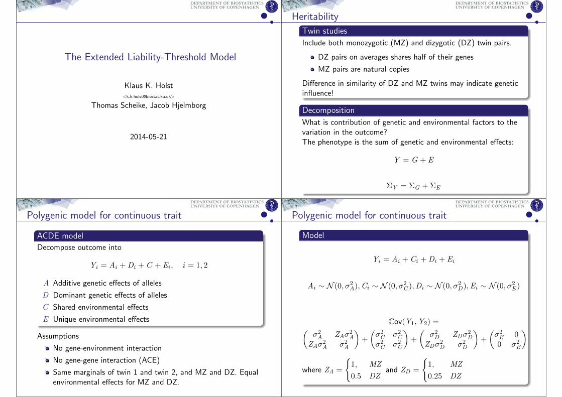
Polygenic model for continuous trait
ACDE model
Decompose outcome into
Yi = Ai + Di + C + Ei , i = 1, 2
A Additive genetic effects of alleles
D Dominant genetic effects of alleles
C Shared environmental effects
E Unique environmental effects
Assumptions
No gene-environment interaction
No gene-gene interaction (ACE)
Same marginals of twin 1 and twin 2, and MZ and DZ. Equalenvironmental effects for MZ and DZ.
UNIVERSITY OF COPENHAGENDEPARTMENT OF BIOSTATISTICS
Polygenic model for continuous trait
Model
Yi = Ai + Ci + Di + Ei
Ai ∼ N (0, σ2A),Ci ∼ N (0, σ2C ),Di ∼ N (0, σ2D),Ei ∼ N (0, σ2E )
Cov(Y1,Y2) =(
σ2A ZAσ2A
ZAσ2A σ2A
)+
(σ2C σ2Cσ2C σ2C
)+
(σ2D ZDσ
2D
ZDσ2D σ2D
)+
(σ2E 00 σ2E
)
where ZA =
{1, MZ
0.5 DZand ZD =
{1, MZ
0.25 DZ
UNIVERSITY OF COPENHAGENDEPARTMENT OF BIOSTATISTICS
Polygenic model
A1 D1 E1 C A2 D2 E2
Y1 Y2
X Z
λA
λDλE
λCλA
λD
λEλC
DZ0.5/
MZ1
DZ0.25/
MZ1
UNIVERSITY OF COPENHAGENDEPARTMENT OF BIOSTATISTICS
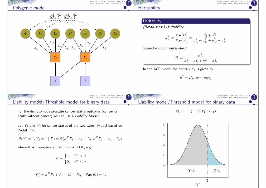
Heritability
Heritability
(Broad-sense) Heritability
h2Y =
Var(G)
Var(Y )=
σ2A + σ2Dσ2A + σ2C + σ2D + σ2E
Shared environmental effect
c2Y =σ2C
σ2A + σ2C + σ2D + σ2E
In the ACE model the heritability is given by
h2 = 2(ρMZ − ρDZ )
UNIVERSITY OF COPENHAGENDEPARTMENT OF BIOSTATISTICS
Liability model/Threshold model for binary data
For the dichotomous prostate cancer status outcome (cancer ordeath without cancer) we can use a Liability Model
Let Y1 and Y2 be cancer status of the two twins. Model based onProbit link:
P(Y1 = 1,Y2 = 1 | X ) = Φ(βTX1 + A1 + C1, βTX2 + A2 + C2)
where Φ is bivariate standard normal CDF, e.g.
Yi =
{1, Y ∗
i > 0
0, Y ∗i ≤ 0
Y ∗i = βTXi + Ai + Ci + Ei , Var(Ei) = 1.
UNIVERSITY OF COPENHAGENDEPARTMENT OF BIOSTATISTICS
Liability model/Threshold model for binary data
P(Y1 = 1) = P(Y ∗1 > τ1)
Y*
0.0
0.1
0.2
0.3
0.4
τ
Y=0 Y=1
UNIVERSITY OF COPENHAGENDEPARTMENT OF BIOSTATISTICS
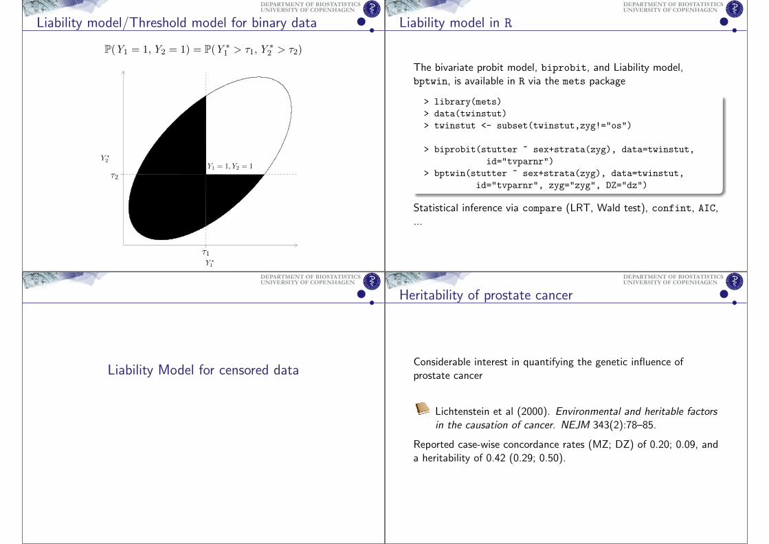
Liability model/Threshold model for binary data
P(Y1 = 1,Y2 = 1) = P(Y ∗1 > τ1,Y
∗2 > τ2)
Y ∗1
Y ∗2
τ1
τ2Y1 = 0, Y2 = 0 Y1 = 1, Y2 = 0
Y1 = 0, Y2 = 1 Y1 = 1, Y2 = 1
UNIVERSITY OF COPENHAGENDEPARTMENT OF BIOSTATISTICS
Liability model in R
The bivariate probit model, biprobit, and Liability model,bptwin, is available in R via the mets package
> library(mets)
> data(twinstut)
> twinstut <- subset(twinstut,zyg!="os")
> biprobit(stutter ~ sex+strata(zyg), data=twinstut,
id="tvparnr")
> bptwin(stutter ~ sex+strata(zyg), data=twinstut,
id="tvparnr", zyg="zyg", DZ="dz")
Statistical inference via compare (LRT, Wald test), confint, AIC,...
UNIVERSITY OF COPENHAGENDEPARTMENT OF BIOSTATISTICS
Liability Model for censored data
UNIVERSITY OF COPENHAGENDEPARTMENT OF BIOSTATISTICS
Heritability of prostate cancer
Considerable interest in quantifying the genetic influence ofprostate cancer
Lichtenstein et al (2000). Environmental and heritable factorsin the causation of cancer. NEJM 343(2):78–85.
Reported case-wise concordance rates (MZ; DZ) of 0.20; 0.09, anda heritability of 0.42 (0.29; 0.50).
UNIVERSITY OF COPENHAGENDEPARTMENT OF BIOSTATISTICS
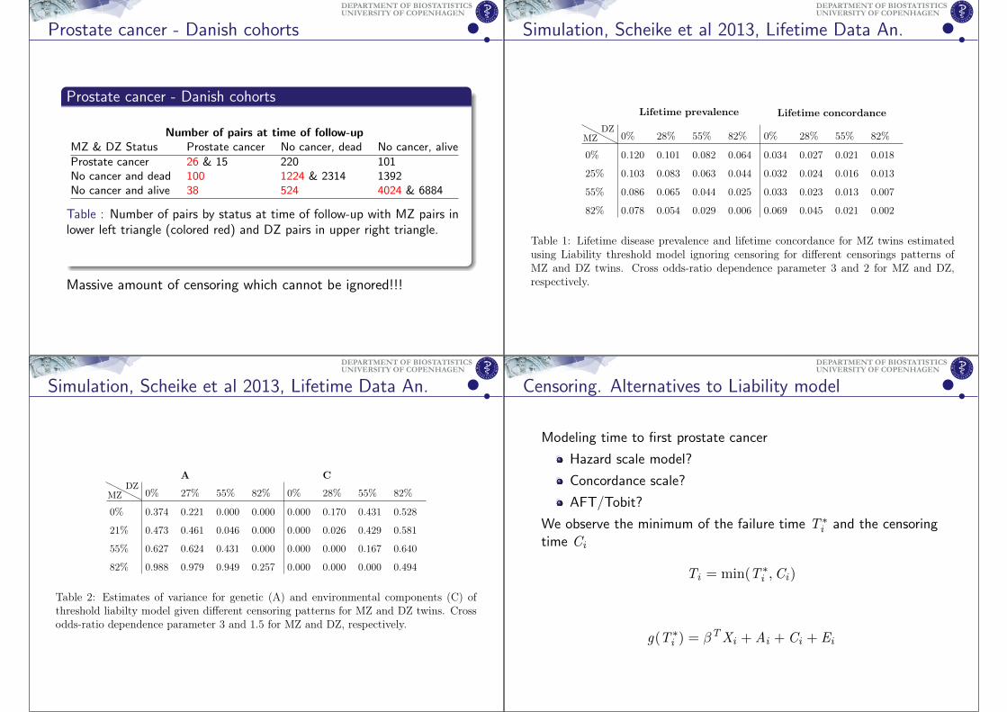
Prostate cancer - Danish cohorts
Prostate cancer - Danish cohorts
Number of pairs at time of follow-upMZ & DZ Status Prostate cancer No cancer, dead No cancer, alive
Prostate cancer 26 & 15 220 101No cancer and dead 100 1224 & 2314 1392No cancer and alive 38 524 4024 & 6884
Table : Number of pairs by status at time of follow-up with MZ pairs inlower left triangle (colored red) and DZ pairs in upper right triangle.
Massive amount of censoring which cannot be ignored!!!
UNIVERSITY OF COPENHAGENDEPARTMENT OF BIOSTATISTICS
Simulation, Scheike et al 2013, Lifetime Data An.
MZDZ
0% 28% 55% 82% 0% 28% 55% 82%
0% 0.120 0.101 0.082 0.064 0.034 0.027 0.021 0.018
25% 0.103 0.083 0.063 0.044 0.032 0.024 0.016 0.013
55% 0.086 0.065 0.044 0.025 0.033 0.023 0.013 0.007
82% 0.078 0.054 0.029 0.006 0.069 0.045 0.021 0.002
Lifetime prevalence Lifetime concordance
Table 1: Lifetime disease prevalence and lifetime concordance for MZ twins estimatedusing Liability threshold model ignoring censoring for different censorings patterns ofMZ and DZ twins. Cross odds-ratio dependence parameter 3 and 2 for MZ and DZ,respectively.
A C
MZDZ
0% 27% 55% 82% 0% 28% 55% 82%
0% 0.374 0.221 0.000 0.000 0.000 0.170 0.431 0.528
21% 0.473 0.461 0.046 0.000 0.000 0.026 0.429 0.581
55% 0.627 0.624 0.431 0.000 0.000 0.000 0.167 0.640
82% 0.988 0.979 0.949 0.257 0.000 0.000 0.000 0.494
Table 2: Estimates of variance for genetic (A) and environmental components (C) ofthreshold liabilty model given different censoring patterns for MZ and DZ twins. Crossodds-ratio dependence parameter 3 and 1.5 for MZ and DZ, respectively.
A C
MZDZ
0% 28% 55% 82% 0% 28% 55% 82%
0% 0.316 0.024 0.000 0.000 0.079 0.367 0.454 0.530
21% 0.513 0.255 0.000 0.000 0.000 0.229 0.496 0.585
55% 0.676 0.633 0.253 0.000 0.000 0.019 0.341 0.646
82% 0.990 0.981 0.954 0.179 0.000 0.000 0.000 0.578
Table 3: Estimates of variance for genetic (A) and environmental components (C) ofthreshold liabilty model given different censoring patterns for MZ and DZ twins. Crossodds-ratio dependence parameter 3 and 2 for MZ and DZ, respectively.
23
UNIVERSITY OF COPENHAGENDEPARTMENT OF BIOSTATISTICS
Censoring. Alternatives to Liability model
Modeling time to first prostate cancer
Hazard scale model?
Concordance scale?
AFT/Tobit?
We observe the minimum of the failure time T ∗i and the censoring
time Ci
Ti = min(T ∗i ,Ci)
g(T ∗i ) = βTXi + Ai + Ci + Ei
UNIVERSITY OF COPENHAGENDEPARTMENT OF BIOSTATISTICS
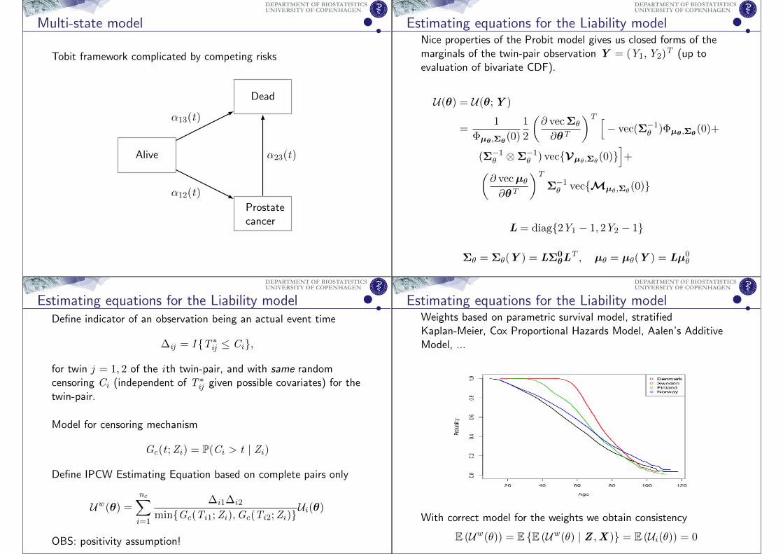
Multi-state model
Tobit framework complicated by competing risks
Dead
Alive
Prostatecancer
α13(t)
α12(t)
α23(t)
UNIVERSITY OF COPENHAGENDEPARTMENT OF BIOSTATISTICS
Estimating equations for the Liability modelNice properties of the Probit model gives us closed forms of themarginals of the twin-pair observation Y = (Y1,Y2)
T (up toevaluation of bivariate CDF).
U(θ) = U(θ;Y )
=1
Φµθ ,Σθ(0)
1
2
(∂ vecΣθ
∂θT
)T [− vec(Σ−1
θ )Φµθ ,Σθ(0)+
(Σ−1θ ⊗Σ−1
θ ) vec{Vµθ,Σθ(0)}
]+
(∂ vecµθ∂θT
)T
Σ−1θ vec{Mµθ,Σθ
(0)}
L = diag{2Y1 − 1, 2Y2 − 1}
Σθ = Σθ(Y ) = LΣ0θL
T , µθ = µθ(Y ) = Lµ0θ
UNIVERSITY OF COPENHAGENDEPARTMENT OF BIOSTATISTICS
Estimating equations for the Liability modelDefine indicator of an observation being an actual event time
∆ij = I {T ∗ij ≤ Ci},
for twin j = 1, 2 of the ith twin-pair, and with same randomcensoring Ci (independent of T ∗
ij given possible covariates) for thetwin-pair.
Model for censoring mechanism
Gc(t ;Zi) = P(Ci > t | Zi)
Define IPCW Estimating Equation based on complete pairs only
Uw (θ) =
nc∑
i=1
∆i1∆i2
min{Gc(Ti1;Zi),Gc(Ti2;Zi)}Ui(θ)
OBS: positivity assumption!
UNIVERSITY OF COPENHAGENDEPARTMENT OF BIOSTATISTICS
Estimating equations for the Liability modelWeights based on parametric survival model, stratifiedKaplan-Meier, Cox Proportional Hazards Model, Aalen’s AdditiveModel, ...
With correct model for the weights we obtain consistency
E (Uw (θ)) = E {E (Uw (θ) | Z ,X )} = E (Ui(θ)) = 0
UNIVERSITY OF COPENHAGENDEPARTMENT OF BIOSTATISTICS
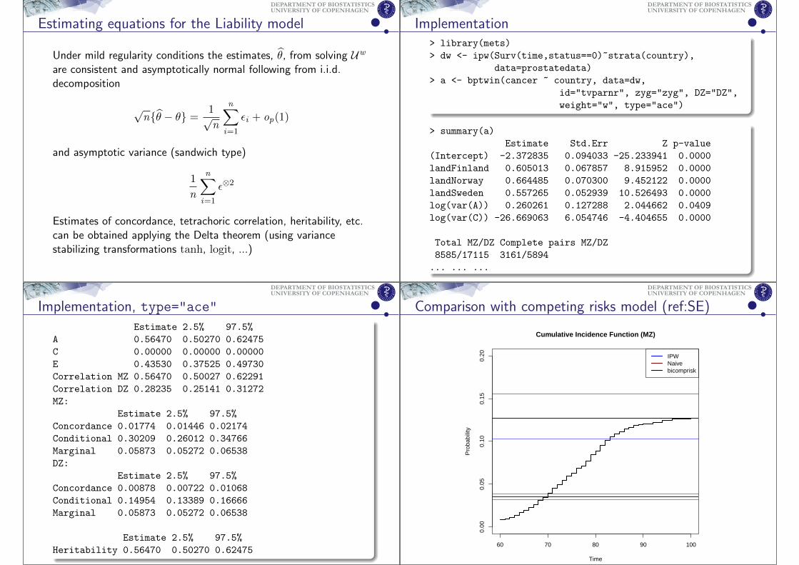
Estimating equations for the Liability model
Under mild regularity conditions the estimates, θ̂, from solving Uw
are consistent and asymptotically normal following from i.i.d.decomposition
√n{θ̂ − θ} =
1√n
n∑
i=1
εi + op(1)
and asymptotic variance (sandwich type)
1
n
n∑
i=1
ε⊗2
Estimates of concordance, tetrachoric correlation, heritability, etc.can be obtained applying the Delta theorem (using variancestabilizing transformations tanh, logit, ...)
UNIVERSITY OF COPENHAGENDEPARTMENT OF BIOSTATISTICS
Implementation> library(mets)
> dw <- ipw(Surv(time,status==0)~strata(country),
data=prostatedata)
> a <- bptwin(cancer ~ country, data=dw,
id="tvparnr", zyg="zyg", DZ="DZ",
weight="w", type="ace")
> summary(a)
Estimate Std.Err Z p-value
(Intercept) -2.372835 0.094033 -25.233941 0.0000
landFinland 0.605013 0.067857 8.915952 0.0000
landNorway 0.664485 0.070300 9.452122 0.0000
landSweden 0.557265 0.052939 10.526493 0.0000
log(var(A)) 0.260261 0.127288 2.044662 0.0409
log(var(C)) -26.669063 6.054746 -4.404655 0.0000
Total MZ/DZ Complete pairs MZ/DZ
8585/17115 3161/5894
... ... ...
UNIVERSITY OF COPENHAGENDEPARTMENT OF BIOSTATISTICS
Implementation, type="ace"
Estimate 2.5% 97.5%
A 0.56470 0.50270 0.62475
C 0.00000 0.00000 0.00000
E 0.43530 0.37525 0.49730
Correlation MZ 0.56470 0.50027 0.62291
Correlation DZ 0.28235 0.25141 0.31272
MZ:
Estimate 2.5% 97.5%
Concordance 0.01774 0.01446 0.02174
Conditional 0.30209 0.26012 0.34766
Marginal 0.05873 0.05272 0.06538
DZ:
Estimate 2.5% 97.5%
Concordance 0.00878 0.00722 0.01068
Conditional 0.14954 0.13389 0.16666
Marginal 0.05873 0.05272 0.06538
Estimate 2.5% 97.5%
Heritability 0.56470 0.50270 0.62475
UNIVERSITY OF COPENHAGENDEPARTMENT OF BIOSTATISTICS
Comparison with competing risks model (ref:SE)
60 70 80 90 100
0.00
0.05
0.10
0.15
0.20
Cumulative Incidence Function (MZ)
Time
Pro
babi
lity
IPWNaivebicomprisk

UNIVERSITY OF COPENHAGENDEPARTMENT OF BIOSTATISTICS
Comparison with bivariate competing risks model
55 60 65 70 75 80 85 90
0.00
0.01
0.02
0.03
0.04
0.05
0.06
Time
Pro
babi
lity
Concordance Prostate cancer (MZ)
bptwinbicomprisk
UNIVERSITY OF COPENHAGENDEPARTMENT OF BIOSTATISTICS
Implementation. type="cor"
Estimate 2.5% 97.5%
Correlation MZ 0.56718 0.49546 0.63121
Correlation DZ 0.27713 0.20442 0.34680
MZ:
Estimate 2.5% 97.5%
Concordance 0.01784 0.01441 0.02207
Conditional 0.30378 0.25774 0.35413
Marginal 0.05872 0.05271 0.06537
DZ:
Estimate 2.5% 97.5%
Concordance 0.00865 0.00661 0.01132
Conditional 0.14736 0.11868 0.18154
Marginal 0.05872 0.05271 0.06537
Estimate 2.5% 97.5%
Heritability 0.58009 0.38028 0.75669
UNIVERSITY OF COPENHAGENDEPARTMENT OF BIOSTATISTICS
Implementation. type="flex"
Estimate 2.5% 97.5%
Correlation MZ 0.57110 0.49992 0.63462
Correlation DZ 0.27485 0.20253 0.34419
MZ:
Estimate 2.5% 97.5%
Concordance 0.01854 0.01369 0.02507
Conditional 0.30886 0.25980 0.36266
Marginal 0.06003 0.04953 0.07258
DZ:
Estimate 2.5% 97.5%
Concordance 0.00845 0.00629 0.01136
Conditional 0.14546 0.11645 0.18022
Marginal 0.05811 0.05099 0.06615
Estimate 2.5% 97.5%
Heritability 0.59250 0.39270 0.76577
UNIVERSITY OF COPENHAGENDEPARTMENT OF BIOSTATISTICS
R Implementation
Stratified analysis
> a <- bptwin(cancer ~ strata(country), data=dw,
id="tvparnr", zyg="zyg", DZ="DZ",
weight="w", type="cor")
Optimization
> mean(score(a)^2) ## Close to zero?
> a$opt ## Messages from optimization routime
> a <- bptwin(..., control=list(trace=1,iter.max=100,
start=mystart,grtol=1e-10,...))
UNIVERSITY OF COPENHAGENDEPARTMENT OF BIOSTATISTICS
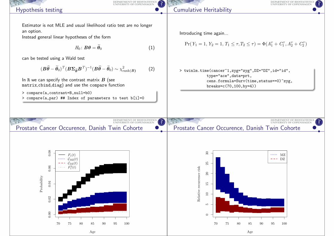
Hypothesis testing
Estimator is not MLE and usual likelihood ratio test are no longeran option.Instead general linear hypotheses of the form
H0 : Bθ = θ̃0 (1)
can be tested using a Wald test
(B θ̂ − θ̃0)T (BΣ
θ̂BT )−1(B θ̂ − θ̃0) ∼ χ2
rank(B) (2)
In R we can specify the contrast matrix B (seematrix,cbind,diag) and use the compare function
> compare(a,contrast=B,null=b0)
> compare(a,par) ## Index of parameters to test b[i]=0
UNIVERSITY OF COPENHAGENDEPARTMENT OF BIOSTATISTICS
Cumulative Heritability
Introducing time again...
Pr(Y1 = 1,Y2 = 1,T1 ≤ τ,T2 ≤ τ) = Φ(Aτ1 + C τ1 ,A
τ2 + C τ
2 )
> twinlm.time(cancer~1,zyg="zyg",DZ="DZ",id="id",
type="ace",data=prt,
cens.formula=Surv(time,status==0)~zyg,
breaks=c(70,100,by=4))
UNIVERSITY OF COPENHAGENDEPARTMENT OF BIOSTATISTICS
Prostate Cancer Occurence, Danish Twin Cohorte
70 75 80 85 90 95 100
0.00
0.02
0.04
0.06
0.08
Age
Probab
ility
F1(t)CMZ(t)CDZ(t)F 21 (t)
UNIVERSITY OF COPENHAGENDEPARTMENT OF BIOSTATISTICS
Prostate Cancer Occurence, Danish Twin Cohorte
70 75 80 85 90 95 100
05
1015
2025
30
Age
Relativerecurrence
risk
MZDZ
UNIVERSITY OF COPENHAGENDEPARTMENT OF BIOSTATISTICS
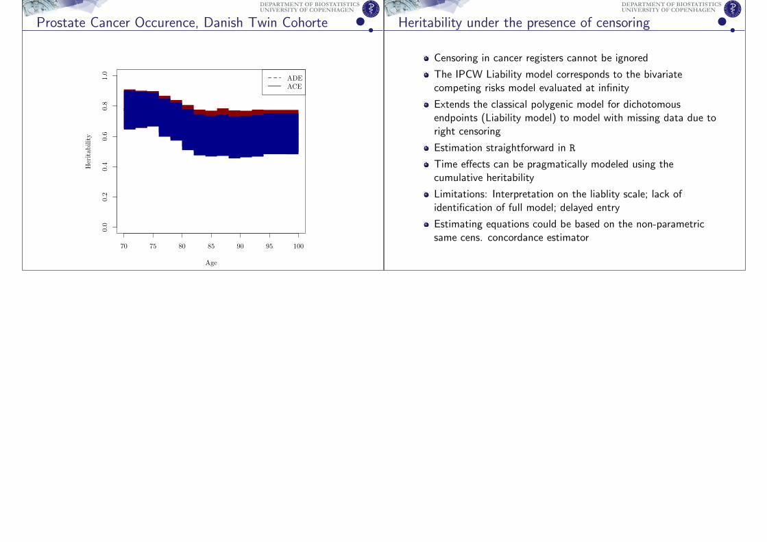
Prostate Cancer Occurence, Danish Twin Cohorte
70 75 80 85 90 95 100
0.0
0.2
0.4
0.6
0.8
1.0
Age
Heritability
ADEACE
UNIVERSITY OF COPENHAGENDEPARTMENT OF BIOSTATISTICS
Heritability under the presence of censoring
Censoring in cancer registers cannot be ignored
The IPCW Liability model corresponds to the bivariatecompeting risks model evaluated at infinity
Extends the classical polygenic model for dichotomousendpoints (Liability model) to model with missing data due toright censoring
Estimation straightforward in R
Time effects can be pragmatically modeled using thecumulative heritability
Limitations: Interpretation on the liablity scale; lack ofidentification of full model; delayed entry
Estimating equations could be based on the non-parametricsame cens. concordance estimator