henrique s. basso and omar rachedi - bde
TRANSCRIPT

THE YOUNG, THE OLD, AND THE GOVERNMENT: DEMOGRAPHICS AND FISCAL MULTIPLIERS
Henrique S. Basso and Omar Rachedi
Documentos de Trabajo N.º 1837
2018

THE YOUNG, THE OLD, AND THE GOVERNMENT: DEMOGRAPHICS
AND FISCAL MULTIPLIERS

THE YOUNG, THE OLD, AND THE GOVERNMENT:
DEMOGRAPHICS AND FISCAL MULTIPLIERS (*)
Henrique S. Basso and Omar Rachedi
BANCO DE ESPAÑA
Documentos de Trabajo. N.º 1837
2018
(*) Addresses: [email protected] and [email protected]. The views expressed in this paper are those of the authors and do not necessarily represent the views of the Banco de España or the Eurosystem. We thank Florian Bilbiie, Jesús Fernández-Villaverde, Basile Grassi, Alexandre Janiak, Matthias Kredler, Alexander Ludwig, Alisdair McKay, Claudio Michelacci, Nicola Pavoni, William Peterman, Emiliano Santoro, Ctirad Slavik, Harald Uhlig, Ernesto Villanueva, Minchul Yum, and presentation participants at the Pontificia Universidad Católica de Chile, University of Copenhagen, Bank of Canada, Federal Reserve Bank of New York, Stony Brook University, CEFER at the Bank of Lithuania, CERGE-EI, Universidad Carlos III de Madrid, University of Glasgow, Banco de Portugal, Latvijas Banka, the RES Conference in Bristol, the IBEO Workshop in Alghero, the CEF Conference in New York, the EEA-ESEM Meeting in Lisbon, the Money Macro and Finance Conference in London, the Macro Banking and Finance Workshop in Milan, the ESCB Research Cluster Workshop on “Medium and long-run challenges for Europe”, the SAEe Meeting in Barcelona, the Workshop on Fiscal Policy in EMU: The Way Ahead in Frankfurt, the Conference on Theories and Methods in Macroeconomics in Paris, the CEPR Conference on “Growth and inequality: long-term effects of short-term policies” in Tel Aviv, the Bristol Macro Workshop, the World Bank-Banco de España Conference on “Output fluctuations and long-term growth” in Madrid, the Portuguese Economic Journal Conference in Lisbon, the Conference on “Growth and business cycle in theory and practice” in Manchester, and the LuBraMacro Workshop in Aveiro for useful comments and suggestions.

The Working Paper Series seeks to disseminate original research in economics and fi nance. All papers have been anonymously refereed. By publishing these papers, the Banco de España aims to contribute to economic analysis and, in particular, to knowledge of the Spanish economy and its international environment.
The opinions and analyses in the Working Paper Series are the responsibility of the authors and, therefore, do not necessarily coincide with those of the Banco de España or the Eurosystem.
The Banco de España disseminates its main reports and most of its publications via the Internet at the following website: http://www.bde.es.
Reproduction for educational and non-commercial purposes is permitted provided that the source is acknowledged.
© BANCO DE ESPAÑA, Madrid, 2018
ISSN: 1579-8666 (on line)

Abstract
We document that fi scal multipliers depend on the age structure of the population. Using
the variation in military spending and birth rates across U.S. states, we show that local fi scal
multipliers increase with the share of young people in total population. We rationalize this
fact with a parsimonious life-cycle open-economy New Keynesian model with credit market
imperfections. The model explains 65% of the relationship between local fi scal multipliers
and demographics. We use the model to study the implications of population aging, and
fi nd that nowadays U.S. national fi scal multipliers are 36% lower than in 1980.
Keywords: life-cycle, population aging, fi scal policy.
JEL classifi cation: E30, E62, J11.

Resumen
Este artículo muestra que el tamaño del multiplicador fi scal depende de la estructura demo-
gráfi ca de la población de una economía. Usando la variación en el gasto militar y las tasas
de natalidad en los estados de Estados Unidos, mostramos que los multiplicadores fi scales
locales aumentan con la proporción de jóvenes en la población total. Racionalizamos este
hecho con un parsimonioso modelo neokeynesiano de economía abierta, y con generaciones
solapadas e imperfecciones del mercado crediticio. El modelo explica el 65 % de la relación
entre los multiplicadores fi scales locales y la demografía. Usamos el modelo para estudiar
las implicaciones del envejecimiento de la población y encontramos que en la actualidad los
multiplicadores fi scales nacionales de Estados Unidos son un 36 % más bajos que en 1980.
Palabras clave: generaciones solapadas, envejecimiento de la población, política fi scal.
Códigos JEL: E30, E62, J11.
BANCO DE ESPAÑA 7 DOCUMENTO DE TRABAJO N.º 1837
1 Introduction
Every time a government considers a plan of fiscal stimulus or fiscal consolidation,
there is a strong debate among policymakers, journalists, and economists on the
effectiveness of such a policy. This effectiveness is often summarized by the size of
the fiscal multiplier, which measures by how much output expands following a rise
in government spending. Nevertheless, fiscal multipliers are not constant structural
parameters, but rather they depend on the characteristics of the economy.
This paper sheds light on a novel determinant of the size of the government
spending multiplier: the age structure of an economy. We study a panel of output,
military spending, and demographic characteristics across U.S. states and document
that local fiscal multipliers rise with the share of young people in total population.
We show that a parsimonious life-cycle open-economy New Keynesian model with
credit market imperfections explains 65% of the link between local fiscal multipliers
and demographics. Then, we use the model to study the implications of population
aging and find that nowadays U.S. national government spending multipliers are
36% lower than in 1980.
We focus on the differences across U.S. states to uncover the causal effect of
demographics on fiscal multipliers. The identification comes from the cross-state
variation in the share of young people in total population. As states’ age structure
can respond to government spending shocks through migration flows, we exploit the
heterogeneity in fertility across U.S. states and instrument the share of young people
with lagged birth rates. Then, we identify the government spending shocks by using
the geographical distribution of government military spending, as in Nakamura and
Steinsson (2014). Usually, the literature on national military spending and fiscal
multipliers identifies government spending shocks by assuming that the U.S. do not
embark in a war when national output is low (Barro, 1981; Barro and Redlick, 2011;
Ramey, 2011). Instead, we refer to a much weaker exogeneity restriction and posit
that the U.S. do not embark in a war when the output of a specific state is lower
than the output of all the other states. Importantly, the geographical distribution of

BANCO DE ESPAÑA 8 DOCUMENTO DE TRABAJO N.º 1837
military spending is uncorrelated with the age structure across states, corroborating
our identification approach.
In our benchmark regression, the size of fiscal multipliers depends positively
on the share of young people (aged 20 - 29) in total population: increasing the
share of young people by 1% above the average share across U.S. states raises the
local output fiscal multiplier by 3.1%, from 1.51 up to 1.56. These estimates imply
an inter-quantile range of output fiscal multipliers across U.S. states that varies
between 1.27 and 1.65. We run a comprehensive battery of robustness checks and
find that the age sensitivity of local fiscal multipliers is always highly economically
and statistically significant. In particular, we show that the age-sensitivity of local
fiscal multipliers holds above and beyond any effect that differences across states
in the unemployment rates, the Gini indexes of labor earnings, and the sectoral
compositions of value added - among other variables - have on the propagation of
military spending on output.
To rationalize the link between demographics and fiscal multipliers, we build a
life-cycle open-economy New Keynesian model with credit market imperfections.
We consider a staggered price setting model with two countries that belong to a
monetary union. The household sector has a life-cycle structure, whereby individ-
uals face three stages of life: young, mature, and old. Following Gertler (1999),
we define a framework in which the optimal choices of the individuals within each
age group aggregate linearly. Although this approach reduces the relevance of dif-
ferences within age groups, it allows us to emphasize the heterogeneity across age
groups and incorporate nominal rigidities and open economy interactions into a
tractable environment. In this way, our model extends a standard two-country New
Keynesian economy with a rich life-cycle structure.
The model features credit market imperfections. Households can trade capital
and bonds but cannot perfectly smooth consumption because markets are incom-
plete. In the baseline model, we restrict further households’ borrowing capacity
with an ad-hoc constraint which does not allow any borrowing at all.

BANCO DE ESPAÑA 9 DOCUMENTO DE TRABAJO N.º 1837
In the model government spending triggers an negative wealth effect for the
households, which smooth consumption by working longer hours. The way in which
the rise in labor earnings affects the response of consumption - and thus the size of
fiscal multipliers - depends on households’ marginal propensity to consume. More-
over, price rigidities define a demand channel through which government spending
raises output even further.
How can demographics alter fiscal multipliers? An economy with relatively more
young households features a stronger demand channel. Since young households
face a hump-shaped labor income over the life-cycle, they want to borrow and
smooth lifetime consumption. Yet, this mechanism is limited by the presence of
credit market imperfections, which boost the marginal propensity to consume of
young households well above the one of mature households, as it is in the data.1
Consequently, as the proportion of young workers increases, output reacts more
sharply to a fiscal shock.
In the quantitative analysis, the model explains entirely the size of fiscal multi-
pliers and 65% of the link between fiscal multipliers and demographics: increasing
the share of young people by 1% above the average share across U.S. states raises
the local output fiscal multiplier by 2%, from 1.51 up to 1.54. We then measure the
contribution of the two forms of credit market imperfections on the results of the
baseline model. We do so by considering a counterfactual economy in which there is
no ad-hoc borrowing constraint and young households can borrow. In this case, the
age sensitivity of the local fiscal multiplier equals 1%. This result points out that
the lack of complete markets in a life-cycle setting can generate the age sensitivity
1Young households have a number of characteristics associated with a higher marginal propensity to consume.For instance, young households own much less liquid assets than older households and the marginal propensityto consume depends negatively on the amount of liquid assets (Kaplan et al., 2014; Misra and Surico, 2014).
of local multipliers, even in absence of the ad-hoc borrowing constraint.
Does the link between demographics and fiscal multipliers exist also at the na-
tional level? Although our evidence shows that the effect of demographics on fiscal
multipliers at the state level is economically and statistically significant, this result

BANCO DE ESPAÑA 10 DOCUMENTO DE TRABAJO N.º 1837
does not necessarily imply that demographics alter also national multipliers.2 We
evaluate in the model the effects of government spending on national output and
find that demographics still matter: increasing the share of young people by 1%
raises the national output fiscal multiplier by 1.1%.
Finally, we study the implications of the U.S. population aging for fiscal policy.
After the post-World War II baby boom, the demographic structure of the U.S.
population has progressively shifted towards older ages: the share of young people
in total population plummeted by 30% from 1980 to 2015. Once we feed this shift in
population shares into our model, we find that nowadays the national output fiscal
multiplier is 36% lower than forty years ago. Since most advanced economies are
experiencing a gradual population aging, the model suggests that over time fiscal
policy could become a relatively less effective tool to spur economy activity.3
This paper is related to the literature that focuses on the implications of demo-
graphics for long-run trends (Krueger and Ludwig, 2007; Aksoy et al., 2018; Car-
valho et al., 2016), and short-term fluctuations (Jaimovich and Siu, 2009; Wong,
2016). The implications of demographics for the aggregate effects of fiscal pol-
icy have been highlighted by Anderson et al. (2016), Janiak and Santos-Monteiro
(2016), and Ferraro and Fiori (2017). Our paper differs from this strand of the lit-
erature on two main dimensions. First, we focus on the elasticity of output to fiscal
shocks. Following Nakamura and Steinsson (2014) and Chodorow-Reich (2018), we
2Nakamura and Steinsson (2014) and Chodorow-Reich (2017) show that local fiscal multipliers considerthe local impact of federally financed policies and wash out any monetary policy response to governmentspending. Both features make local multipliers larger than national ones. On the other hand, local multipliersare dampened by expenditure switching and import leakage effects that do not take place at the national level.
3This result refers to the effectiveness of fiscal policy in normal times. The literature has highlighted casesin which fiscal multipliers are very high, e.g., when the economy is at zero lower bound (Christiano et al., 2011;Woodford, 2011) or there is slack in the economy (Auerbach and Gorodnichenko, 2012; Rendahl, 2016).
exploit the heterogeneity across U.S. states and estimate the causal effect of demo-
graphics on fiscal multipliers.4 Second, we build a quantitative model that can be
used as a laboratory to measure the effects of changes in the age structure of the
economy on fiscal multipliers.
4Anderson et al. (2016) and Ferraro and Fiori (2017) derive the responses of consumption and unemploymentacross age groups to national fiscal shocks identified with the narrative approach of Romer and Romer (2010).

BANCO DE ESPAÑA 11 DOCUMENTO DE TRABAJO N.º 1837
2 Empirical Evidence
This Section shows that local fiscal multipliers depend on demographics: fiscal
multipliers are larger in states with higher shares of young people in total population.
We study a panel of output, government military spending, and demographic
characteristics across U.S. states. To estimate the effect of government spending
on output - and how this effect depends on the age structure of each state - we
use the variation across U.S. states in both military buildups and birth rates. This
procedure identifies the local fiscal multiplier, which is a federally-financed open-
economy relative multiplier. This multiplier estimates the response of output in a
specific state (say, California) relative to the response of output of all the other U.S.
states when the federal government spends one extra dollar in California, and this
dollar is financed by taxing individuals in all U.S. states.
2.1 Data
We build a data set of government military spending, output, and demographic
characteristics across the 50 U.S. states and the District of Columbia at the annual
frequency from 1967 until 2015.
We complement the data on the geographical distribution of military spending
of Nakamura and Steinsson (2014) with information from the Statistical Abstract
of the U.S. Census Bureau and the website usaspending.org of the U.S. Office of
Management and Budget. The data cover any procurement of the U.S. Department
of Defense above 10,000$ up to 1983, and above 25,000$ from 1983 on.5
State output is the state GDP series of the Bureau of Economic Analysis (BEA).
State employment is taken from the Current Employment Statistics of the Bureau of
Labor Statistics (BLS). The data on state population and births rates are from the
Census Bureau. The data on births rates are from 1930 onwards. The birth rates
of Alaska and Hawaii are available only from 1960 onwards. The data on the state
5Nakamura and Steinsson (2014) show that military procurements tend not to be subcontracted to firms indifferent states from the original recipient.

BANCO DE ESPAÑA 12 DOCUMENTO DE TRABAJO N.º 1837
demographic structure by age, race, and sex are from the Survey of Epidemiology
and End Results of the National Cancer Institutes.
2.2 Econometric Specification
We estimate the causal effect of demographics on local output fiscal multipliers using
the following panel regression:
Yi,t − Yi,t−2Yi,t−2
= αi + δt + βGi,t −Gi,t−2
Yi,t−2+ γ
Gi,t −Gi,t−2Yi,t−2
(Di,t − D
)+ ζDi,t + εi,t (1)
where Yi,t denotes per capita output in state i at time t, Gi,t refers to per capita
federal military spending allocated to state i at time t, Di,t is the log-share of young
people over total population in state i at time t multiplied by 100, D =∑
i
∑tDi,t
nint
is the average log-share of young people,6 and ni denotes the number of states and
nt the number of years in the sample. The parameter αi is a state fixed effect, and
δt denotes time fixed effects. The fixed effects capture any state-specific trend in
output, government spending, and demographics, and control for aggregate shocks,
such as variations in the national monetary policy stance.7
6The demeaning of the share of young people allows us to interpret β as the local fiscal multiplier on a statewith the average share of young people, but has no effect whatsoever on the estimation of the age sensitivity γ.
7Following Nakamura and Steinsson (2014), we consider two-year changes in output and government spendingto capture in a parsimonious way the dynamic effects of fiscal policy.
In the baseline regression we consider the share of young people as the ratio of
20-29 years old white males over the total population of white males. We focus on
the white male population to avoid that the different trends across U.S. states in the
labor participation of female workers and workers of other racial groups could be
confounding factors that spuriously drive the effect of changes in the age structure
of the population on the size of local fiscal multipliers. In the robustness checks,
we show that our results do not change if we consider either all males or the entire
population of 20-29 years old individuals.8
In Equation (1) the coefficient β denotes the local output fiscal multiplier: it
defines the dollar increase in per-capita output following a one dollar increase in
8Appendix A.5 shows that lagged births rates are a more relevant instrument for the share of young whitemales rather than for either the share of young males or the share of overall young people.
BANCO DE ESPAÑA 13 DOCUMENTO DE TRABAJO N.º 1837
per-capita federal government spending in a state with the average share of young
people. The parameter γ is associated to our regressor of interest, which is the
interaction between changes in federal government spending and the share of young
people in total population. This parameter defines how fiscal multipliers vary with
the age structure of a state: when the share of young people rises by 1% above the
average, the fiscal multiplier increases from β up to β + γ.
We also estimate the effect of government spending on state employment rate
with a similar regression, in which the dependent variable is the growth rate of state
employment rate Ei,t:
Ei,t − Ei,t−2Ei,t−2
= αi+δt+βGi,t −Gi,t−2
Yi,t−2+γ
Gi,t −Gi,t−2Yi,t−2
(Di,t − D
)+ζDi,t+ εi,t. (2)
We identify government spending shocks following the approach of Nakamura
and Steinsson (2014), which exploits the heterogeneous sensitivity of states’ military
procurements to an increase in federal military spending.9 This IV strategy implies
9E.g., federal military spending as a fraction of national GDP dropped by 1.5% following the U.S. withdrawalfrom Vietnam. The withdrawal had large heterogeneous effects across U.S. states: in California federal militaryprocurements as a fraction of the state GDP decreased by 2.5%, while Illinois experienced a drop of just 1%.
a first stage regression in which per capita state military procurement (as a fraction
of per capita state GDP) is regressed against the product of per capita national
military spending (as a fraction of per capita national GDP) and a state fixed
effect:
Gi,t −Gi,t−2Yi,t−2
= αi + δt + ηiGt −Gt−2
Yt−2+ ϕXi,t + εi,t (3)
where Xi,t includes the instruments for both the share of young people and its
interaction with the changes in government spending. The coefficient ηi captures
the heterogeneous exposure of each state to a rise in federal military spending.
This first stage allows us to capture the systematic fixed state-level sensitivity to
changes in federal spending, which by construction is orthogonal to any variation in
either the political process or the local business cycle that may alter the allocation
of spending across states. Furthermore, from 2000 to 2015 the correlation between
state-level measures of federal military purchases and the spending of local and state
BANCO DE ESPAÑA 14 DOCUMENTO DE TRABAJO N.º 1837
governments is 0.24, suggesting that the bulk of the variation in the allocation of
military spending is not driven by state-specific dynamics.
The use of military spending to estimate national fiscal multipliers follows the
work of Barro (1981), Barro and Redlick (2011), and Ramey (2011), among many
others. This strand of the literature considers national military spending as exoge-
nous. The implicit assumption is that the U.S. do not embark in a war because
national output is low. Our instrumenting approach relies on a much weaker ex-
ogeneity restriction: we posit that the U.S. do not embark in a war because the
output of a specific state is lower relatively to the output of all the other states.
Then, we evaluate whether the effects of government spending shocks on output
and employment depend on states’ age structure. The panel dimension of the data
is crucial to identify the link between demographics and fiscal multipliers. Since
our baseline regression features state and time fixed effects, the identification comes
from the cross-state variation - and its changes over time - in the share of young
people in total population. At any point of time, there is a large dispersion across
states in the share of young people. For instance, in 2015 the share of young people
ranges between the 11.9% of Maine and the 22.6% of D.C. Moreover, the relative
ranking across states has been changing over time. As an example, in 1980 New
York had the fourth lowest share of young people in the U.S. Yet, in 2015 the share
of young people of New York has become the tenth highest in the U.S.
States’ age structure would not be exogenous to government spending shocks if
they trigger migration flows.10 To avoid any concern on the endogeneity of demo-
graphics, we follow Shimer (2001) and instrument the share of young people with
lagged birth rates.11 This IV strategy allows us to identify the causal effect of states’
age structure on fiscal multipliers. In our baseline specification, we instrument the
share of young people with 20-30 year lagged birth rates: we use the average birth
rate between 1940 and 1950 to instrument the share of young people in 1970.12 Fi-
10Blanchard and Katz (1992) show that state migration reacts to shocks. We find that although total popu-lation does not change following government spending shocks, the population of young people does rise.
11Appendix A.5 shows that lagged birth rates explain the bulk of the variability of the age structure of thepopulation across states and time.
12The birth rates for Alaska and Hawaii start in 1960. The results do not change if we consider either anunbalanced panel of birth rates, or we use 10 year lagged birth rates for Alaska and Hawaii.
BANCO DE ESPAÑA 15 DOCUMENTO DE TRABAJO N.º 1837
nally, including the share of young people independently from the interaction with
government spending – through the presence of the term ζDi,t in Equations (1)
and (2) – allows us to control for the potential direct channel whereby changes in
the age-structure of population and fertility rates affect per-capita output. In this
way, the interaction term captures any effect through which demographics shape
the output effects of government spending that hold above and beyond the direct
impact that demographics have on per-capita GDP.
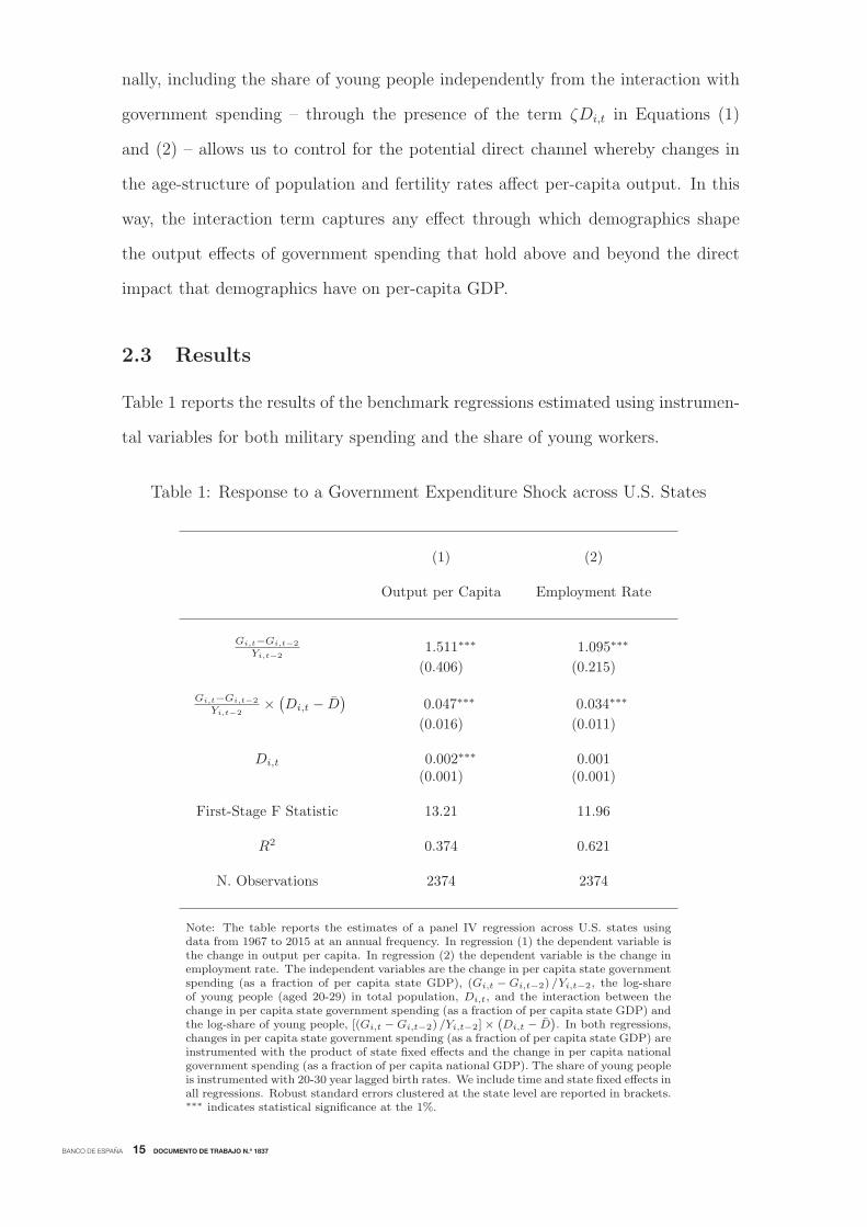
2.3 Results
Table 1 reports the results of the benchmark regressions estimated using instrumen-
tal variables for both military spending and the share of young workers.
Table 1: Response to a Government Expenditure Shock across U.S. States
(1) (2)
Output per Capita Employment Rate
Gi,t−Gi,t−2
Yi,t−21.511∗∗∗ 1.095∗∗∗
(0.406) (0.215)
Gi,t−Gi,t−2
Yi,t−2× (Di,t − D
)0.047∗∗∗ 0.034∗∗∗
(0.016) (0.011)
Di,t 0.002∗∗∗ 0.001(0.001) (0.001)
First-Stage F Statistic 13.21 11.96
R2 0.374 0.621
N. Observations 2374 2374
Note: The table reports the estimates of a panel IV regression across U.S. states usingdata from 1967 to 2015 at an annual frequency. In regression (1) the dependent variable isthe change in output per capita. In regression (2) the dependent variable is the change inemployment rate. The independent variables are the change in per capita state governmentspending (as a fraction of per capita state GDP), (Gi,t −Gi,t−2) /Yi,t−2, the log-shareof young people (aged 20-29) in total population, Di,t, and the interaction between thechange in per capita state government spending (as a fraction of per capita state GDP) andthe log-share of young people, [(Gi,t −Gi,t−2) /Yi,t−2]×
(Di,t − D
). In both regressions,
changes in per capita state government spending (as a fraction of per capita state GDP) areinstrumented with the product of state fixed effects and the change in per capita nationalgovernment spending (as a fraction of per capita national GDP). The share of young peopleis instrumented with 20-30 year lagged birth rates. We include time and state fixed effects inall regressions. Robust standard errors clustered at the state level are reported in brackets.∗∗∗ indicates statistical significance at the 1%.

BANCO DE ESPAÑA 16 DOCUMENTO DE TRABAJO N.º 1837
Column (1) refers to the regression in which the dependent variable is the change
in output per capita. The first entry shows that the local output fiscal multiplier
for a state with an average share of young people (e.g., Massachusetts and Nevada)
is statistically significant at the 1% level and equals 1.51. This result implies that
– in a state with the average share of young people in total population – one addi-
tional dollar of per-capita federal military spending raises per-capita output by 1.51
dollars. Also the estimated value of the parameter γ associated with the interaction
term is highly statistically significant, with a p-value of 0.005. The value of the
estimated parameter points out that the effect of demographics on local output fis-
cal multipliers is also highly economically significant: increasing the share of young
people by 1% above the average raises output fiscal multipliers by 3.1%, from 1.51
up to 1.56. These estimates imply an inter-quantile range of output fiscal multipliers
across U.S. states that varies between the values of 1.27 in Ohio and 1.65 in Arizona.
Column (2) displays the results of the regression in which the dependent variable
is the change in the employment rate. For a state with an average share of young
people, the local employment fiscal multiplier equals 1.10. Demographics affect also
the local employment fiscal multiplier: increasing the share of young people by 1%
in absolute terms above the average raises employment fiscal multipliers by 3.1%,
from 1.10 up to 1.13. Finally, the high values associated with the Kleibergen-Paap
Wald statistic in both regressions – which are also higher than the values of the
partial F-statistic in Nakamura and Steinsson (2014) – corroborate the validity of
our instrumenting strategy.
To assess whether the age sensitivity of local fiscal multipliers hinges on a partic-
ular econometric specification, we run a comprehensive battery of robustness checks.
Table 2 reports the first of alternative specifications for the estimates of both the
local output fiscal multiplier (Panel A) and the local employment fiscal multiplier
(Panel B). In either case, the first column displays the results of the baseline regres-
sion. The following columns show the results for the OLS regression, the “partial”
IV regression in which we instrument state government spending but we do not
instrument the share of young people, an IV regression in which we use a different

BANCO DE ESPAÑA 17 DOCUMENTO DE TRABAJO N.º 1837
measure of young people (those aged 15-29)13, and an IV regression in which we use
a different measure of birth rates (25 years lagged birth rates). Finally, we estimate
the fiscal multipliers in regressions in which the share of young people is computed
over the entire male population and the overall population, rather than using only
the white male population.
The level of the local fiscal multiplier in the baseline regression is fourteen times
larger than the size of the estimate in the OLS regression. The difference in magni-
tude between IV and OLS estimates tend to be analogously large in the entire strand
of the literature on local fiscal multipliers, independently on the instrumenting ap-
proach or the type of government spending or tax under study (e.g., Nakamura
and Steinsson, 2014; Suarez-Serrato and Wingender, 2016; Chodorow-Reich, 2018).
While this finding may be due to the attenuation bias generated by measurement
errors in federal military spending, it also indicates that local military spending
may respond to local conditions, potentially reflecting political pressures. Our in-
strumenting strategy corrects for this bias by focusing on the systematic component
of local spending.
The “partial” IV regression yields an estimated coefficient of the interaction
between changes in government spending and the share of young people which is
larger for the response of output (and smaller for the response of the employment
rate) than in the baseline IV regression. This difference could be driven by the
endogenous reaction of states’ migration flows to a government spending shock. If
migration raises the population, then it would boost further the change in output,
while dampening the response of the employment rate. In Appendix A.3 we confirm
this conjecture by showing that although total population does not change following
a fiscal shock, the population of young people does rise. This evidence strengthen
the relevance of instrumenting the share of young people to avoid any endogeneity
concern driven by state migration flows.
Columns (4) and (5) show that the relationship between demographics and fiscal
multipliers does not hinge on a specific definition of the young group or a specific
instrumenting strategy. Finally, columns (6) and (7) show that the estimated ef-

BANCO DE ESPAÑA 18 DOCUMENTO DE TRABAJO N.º 1837
Table 2: Response of Output & Employment Rate to Government Shocks - Robustness Checks
(1) (2) (3) (4) (5) (6) (7)
Baseline Baseline No IV Share Age Birth Rates All Men Men &Birth Rates 15-29 25 Year Lag Women
IV OLS “Partial” IV IV IV IV IV
Panel A. Response of Output
Gi,t−Gi,t−2
Yi,t−21.511∗∗∗ 0.109 1.515∗∗∗ 1.251∗∗∗ 1.451∗∗∗ 1.664∗∗∗ 1.613∗∗∗
(0.409) (0.112) (0.468) (0.394) (0.396) (0.432) (0.435)
Gi,t−Gi,t−2
Yi,t−2× 0.047∗∗∗ 0.011∗ 0.067∗∗ 0.051∗∗ 0.051∗∗∗ 0.066∗∗ 0.060∗∗
(Di,t − D
)(0.017) (0.006) (0.028) (0.024) (0.017) (0.028) (0.025)
Di,t 0.002∗∗∗ 0.002∗∗∗ 0.002∗∗∗ 0.003∗∗∗ 0.001 0.002∗∗ 0.002∗∗
(0.001) (0.001) (0.001) (0.001) (0.001) (0.001) (0.001)
R2 0.374 0.390 0.330 0.382 0.411 0.362 0.364
N. Observations 2374 2397 2397 2374 2366 2374 2374
Panel B. Response of Employment Rate
Gi,t−Gi,t−2
Yi,t−21.095∗∗∗ 0.180∗∗ 1.046∗∗∗ 0.959∗∗∗ 1.097∗∗∗ 1.091∗∗∗ 1.075∗∗∗
(0.215) (0.076) (0.236) (0.210) (0.210) (0.226) (0.220)
Gi,t−Gi,t−2
Yi,t−2× 0.034∗∗∗ 0.001 0.025∗∗ 0.038∗∗ 0.035∗∗∗ 0.038∗∗ 0.039∗∗
(Di,t − D
)(0.011) (0.005) (0.010) (0.016) (0.010) (0.017) (0.016)
Di,t 0.001 0.001 0.001 0.001∗∗ 0.001 0.001 0.001(0.001) (0.001) (0.001) (0.001) (0.001) (0.001) (0.001)
R2 0.621 0.635 0.590 0.627 0.627 0.625 0.624
N. Observations 2374 2397 2397 2374 2366 2374 2374
Note: The table reports the estimates of panel regressions across U.S. states from 1967 to 2015 at an annual frequency. In PanelA the dependent variable is the change in output per capita. In Panel B the dependent variable is the change in the employmentrate. If not stated otherwise, the independent variables are the change in per capita state government spending (as a fraction ofper capita state GDP), (Gi,t −Gi,t−2) /Yi,t−2, the share of young people (aged 20-29) in total population, Di,t, and the interactionbetween the change in per capita state government spending (as a fraction of per capita state GDP) and the share of young people,[(Gi,t −Gi,t−2) /Yi,t−2]×
(Di,t − D
). In the IV regressions, state-specific changes in per capita state government spending (as a fraction
of per capita state GDP) are instrumented with the product of state fixed effects and the change in per capita national governmentspending (as a fraction of per capita national GDP). The share of young people is instrumented with 20-30 year lagged birth rates.Regression (1) displays the results of the benchmark IV regressions. Regression (2) shows the results of the regression estimated by OLS.In regression (3) we instrument state government spending but we do not instrument the share of young people. In regression (4) we usethe share of the people aged 15-29 in total population as independent variable. In regression (5) we instrument the share of young peoplewith 25 year lagged birth rates. In regression (6) we compute the share of young people not focusing only on white men, but rather onall men. In regression (7) we compute the share of young people not focusing only on white men, but rather on the entire population ofyoung men and women. We include time and state fixed effects in all the regressions. Robust standard errors clustered at the state levelare reported in brackets. ∗, ∗∗, and ∗∗∗ indicate statistical significance at the 10%, 5% and 1%, respectively.

BANCO DE ESPAÑA 19 DOCUMENTO DE TRABAJO N.º 1837
fect of a change in demographics on fiscal multipliers becomes even larger when
computing the share of young people over either the entire male population or the
overall population: a 1% increase in the share of young people rises the size of fiscal
multipliers by around 3.7% - 4%. This pattern is consistent with the fact that white
males have a much lower elasticity of labor supply than females and individuals of
other racial groups.
2.4 Validation of Exclusion Restrictions on Demographics
Our identification of the age-sensitivity of local fiscal multipliers hinges on instru-
menting the current share of young people in total population with lagged birth
rates. Our implicit exclusion restriction posits that, conditional on state and time
fixed effects, whatever determines the cross-sectional variation in births rates has no
other long lasting effect on the size of fiscal multipliers 20-30 years later. Alternative
sources of heterogeneity across states could potentially influence local fiscal multi-
pliers above and beyond the effect of the age structure of the population. However,
in order to violate our restriction these alternative mechanisms must necessarily
display a very narrow set of correlations (within states and within years) with both
current military spending shocks and lagged birth rates.14,15
To validate the exclusion restriction of our IV approach, first we report the
correlation of the share of young people in total population with a number of state-
level key variables which could drive the effects of military spending on output, and
could display dynamics across states and over time similar to the observed changes
in the age structure of the population. Table 3 presents these correlations. The first
confounding factor we consider is the unemployment rate. Young individuals tend
to be relatively more unemployed, and Auerbach and Gorodnichenko (2012) and14We are not concerned about mechanisms that hinge on demographics and affect local fiscal multipliers, such
as the role of changes in the cross-sectional distribution of consumption, labor earnings, and wealth that dependuniquely on the variation in the age structure of the population. Although not all these mechanisms are activein our quantitative model, they still belong to the causal effect of changes in the age structure of the populationon local fiscal multipliers.
15Since we focus on military purchases and does not consider measures of government spending with includestransfers, our estimates can hardly be due to the fact that households in young states have also characteristicswhich make them more likely to be transfer recipients. This claim is further corroborated by the low correlationbetween state-level measures of military purchases and the spending of local and state government, as wemention above.

BANCO DE ESPAÑA 20 DOCUMENTO DE TRABAJO N.º 1837
Nakamura and Steinsson (2014) find that fiscal multipliers may be larger in times of
slack. The demographic transition might also be related to the process of structural
transformation from manufacturing to services, and Bouakez et al. (2018) highlight
that fiscal multipliers depend on the sectoral composition of spending. For this
reason, the second set of variables we study refer to state’s sectoral composition,
and include the share of services value added over total value added, the share of
personal services over total value added and the share of health care services over
total value added. We evaluate also the role of the Gini index of labor earnings as a
potential confounding factor since Brinca et al. (2016) and Hagedorn et al. (2018)
show that the cross-sectional distribution of labor earnings influences the size of
the fiscal multiplier. Then, we consider measures of personal income taxation and
unemployment benefits because the age structure of the population of a state could
also determine its average per-capita amount of taxes and transfers, and Oh and
Reis (2012) argue that the aggregate effects of fiscal policy depend crucially on the
distribution of tax/transfers across households. Finally, we study measures of skilled
labor and female labor participation, as the U.S. economy has experienced dramatic
compositional changes in the labor market which occurred contemporaneously to
the demographic transition towards old ages.
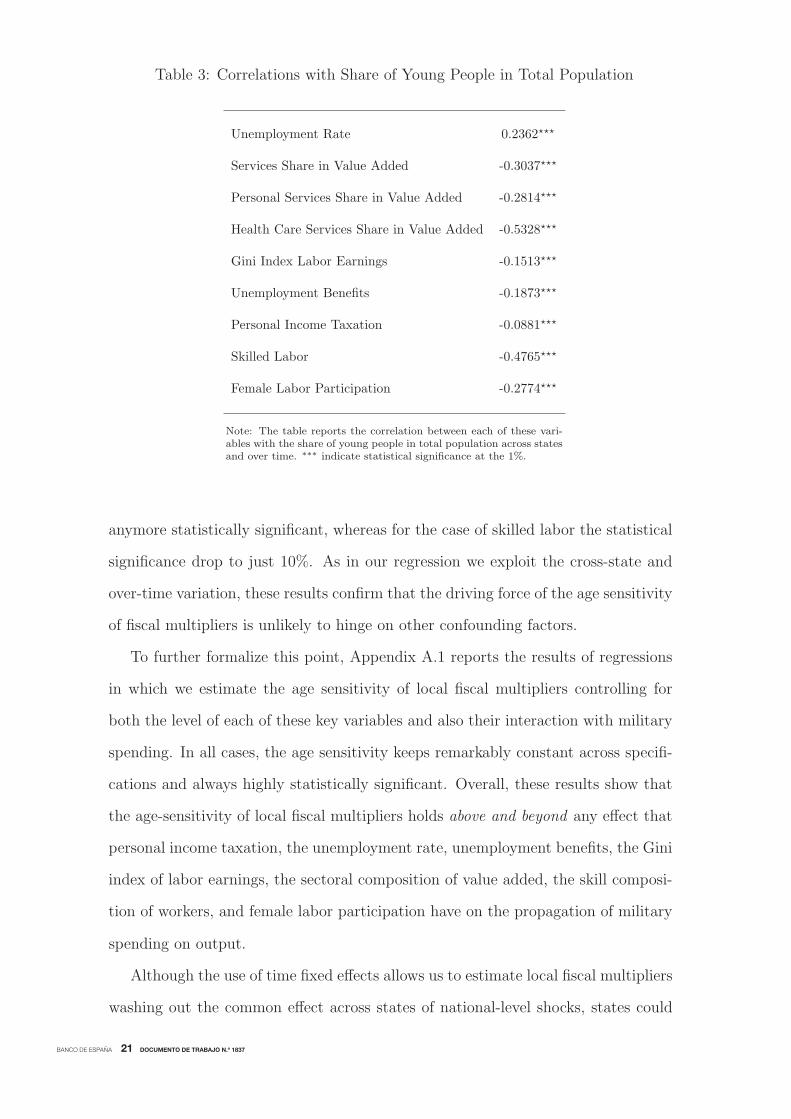
Table 3 shows heterogeneity in the co-movements of these key variables with
the share of young people: the share of health care services in total value added
and the measure of skilled labor have the largest correlations with values around
-0.5, whereas the personal income taxation and the Gini index of labor earnings
have a very weak correlation with the age structure of population, with values
around -0.1. Importantly, even for the two variables with the highest correlations,
the relationship with the share of young people weakens substantially if we run a
simple panel regression that controls also for time and state fixed effects.16 In this
16The share of health care services is likely not to be a relevant confounding factor also because it amountsto just 6% of total value added.
case, the relationship between the health services share and the age structure is not
to be relatively more unemployed, and Auerbach and Gorodnichenko (2012) and
BANCO DE ESPAÑA 21 DOCUMENTO DE TRABAJO N.º 1837
anymore statistically significant, whereas for the case of skilled labor the statistical
significance drop to just 10%. As in our regression we exploit the cross-state and
over-time variation, these results confirm that the driving force of the age sensitivity
of fiscal multipliers is unlikely to hinge on other confounding factors.
To further formalize this point, Appendix A.1 reports the results of regressions
in which we estimate the age sensitivity of local fiscal multipliers controlling for
both the level of each of these key variables and also their interaction with military
spending. In all cases, the age sensitivity keeps remarkably constant across specifi-
cations and always highly statistically significant. Overall, these results show that
the age-sensitivity of local fiscal multipliers holds above and beyond any effect that
personal income taxation, the unemployment rate, unemployment benefits, the Gini
index of labor earnings, the sectoral composition of value added, the skill composi-
tion of workers, and female labor participation have on the propagation of military
Table 3: Correlations with Share of Young People in Total Population
Unemployment Rate 0.2362���
Services Share in Value Added -0.3037���
Personal Services Share in Value Added -0.2814���
Health Care Services Share in Value Added -0.5328���
Gini Index Labor Earnings -0.1513���
Unemployment Benefits -0.1873���
Personal Income Taxation -0.0881���
Skilled Labor -0.4765���
Female Labor Participation -0.2774���
Note: The table reports the correlation between each of these vari-ables with the share of young people in total population across statesand over time. ∗∗∗ indicate statistical significance at the 1%.
spending on output.
Although the use of time fixed effects allows us to estimate local fiscal multipliers
washing out the common effect across states of national-level shocks, states could
BANCO DE ESPAÑA 22 DOCUMENTO DE TRABAJO N.º 1837
17This lack of correlation is also due to the fact that we focus on military procurement data, thus avoiding toconsider items of total government spending (i.e., the public wage bill and the provision of public services andtransfers) that arguably are influenced by the age structure of the population.
display a heterogeneous sensitivity in the response of these common shocks. As
long as this heterogeneity correlates with the evolution of the age structure across
states, this feature would affect the estimate of the age sensitivity of the multiplier.
To address this concern, we introduce additional national-level variables, such as
the change in the oil price, the households’ debt to GDP ratio, the federal debt to
GDP ratio, Ramey (2011) and Ramey and Zubairy (2018)’s series on news about
future increases in government spending, and the real interest rate, and interact all
of them with state fixed effects. The results reported in Appendix A.2 show that the
economic and statistical significance of the age sensitivity of local fiscal multipliers
keep holding even in this case.
Finally, our IV approach would not be valid if the sensitivity to federal govern-
ment shocks - i.e., ηi of Equation (3) - is related to states’ age structure. We find
that in the data the correlation between states’ demographic structures and sensi-
tivity to federal government shocks is -0.03.17 Thus, the geographical distribution
of military spending is not related to demographics, corroborating our identification
approach.

BANCO DE ESPAÑA 23 DOCUMENTO DE TRABAJO N.º 1837
3 The Model
We build a two-country New Keynesian model with a rich, and yet tractable, life-
cycle structure. The two countries - a home and a foreign economy - belong to a
monetary union, with a unique Taylor rule which responds to union-level inflation
and output gap. In the union there is also a federal government which purchases
final consumption goods subject to spending shocks. The government finances its
expenditures by levying lump-sum taxes on the households and issuing bonds.
In each country, the household sector has a life-cycle structure whereby individ-
uals face an idiosyncratic aging risk and live through three stages of life: young,
mature, and old. All the individuals supply labor, accumulate assets, and consume.
The model features credit markets imperfections of two forms: incomplete asset
markets and a borrowing constraint on bond-holdings.
The two countries differ only in the relative size of the population. Hereafter
we just describe the home country. The variables and parameters of the foreign
economy are distinguished by a star superscript.
3.1 Households
In each country there is a continuum of households that belong to three different age
groups: young agents (y), mature agents (m), and old agents (o). The demographic
structure in the home country is described by the measures of young agents Ny,t,
mature agents Nm,t, and old agents No,t such that Ny,t+Nm,t+No,t = Nt. The total
population of the monetary union is NU,t = Nt +N�t .
Agents move through the three different groups of households in a life-cycle
manner as in Yaari (1965) and Blanchard (1985). In the home country, in each
period ωnNy,t new young agents are born and enter the economy. At any given
point of time, households face an idiosyncratic probability to change age groups
in the following period: young agents become mature with a probability 1 − ωy,
mature agents become old with a probability 1− ωm, and old agents die and leave
the economy with a probability 1− ωo.
BANCO DE ESPAÑA 24 DOCUMENTO DE TRABAJO N.º 1837
We can define the law of motion of population across the three age groups as
Ny,t+1 = ωnNy,t + ωyNy,t, (4)
Nm,t+1 = (1− ωy)Ny,t + ωmNm,t, and (5)
No,t+1 = (1− ωm)Nm,t + ωoNo,t. (6)
Individuals face aggregate uncertainty due to fiscal shocks and over the lifetime
they experience three idiosyncratic shocks: the transition from young to mature,
the transition from mature to old, and the exit from the economy. Although agents
are born identical, the idiosyncratic and aggregate uncertainty would generate a
distribution of ex-post heterogeneous households. Following Gertler (1999), we de-
fine a framework in which the optimal choices of the individuals within each age
group aggregate linearly. This approach reduces the relevance of differences het-
erogeneity within age group but it allows us to emphasize the heterogeneity across
age groups and incorporate nominal rigidities and open economy interactions into a
tractable environment. In this way, our model extends a standard two-country New
Keynesian economy with a rich life-cycle structure.
First, we introduce a perfect annuity market which insures old agents against the
risk of death. Old agents transfer their investment in capital and bonds to financial
intermediaries, which pay back the proceedings only to surviving households. Free
entry and perfect competition in the annuity market guarantee a premium to the
return on investment which compensates old agents for the risk of death.
Second, we assume that households are risk neutral. In this way, the uncertainty
on the labor income dynamics due to the transitions from young to mature and
from mature to old, and the aggregate fiscal shocks does not affect optimal choices.
Nevertheless, we keep a motive for consumption smoothing by assuming that in-
dividual preferences belong to the Epstein and Zin (1989) utility family, such that
risk neutrality coexists with a positive elasticity of intertemporal substitution.
At time t the agent i of the age group z = {y,m, o} chooses consumption ciz,t,
labor supply liz,t, capital kiz,t+1, and nominal bonds biz,t+1 to maximize

BANCO DE ESPAÑA 25 DOCUMENTO DE TRABAJO N.º 1837
18Nakamura and Steinsson (2014) show that consumption-labor complementarities are required to matchthe level of the local fiscal multiplier. Gnocchi et al. (2016) study data on time use to document that thecomplementarity between consumption and hours worked is indeed an empirically relevant driver of the responseof labor to a government spending shock. Bilbiie (2011) shows that the consumption-labor complementaritiescan rationalize a positive national consumption fiscal multiplier if prices are not flexible.
19In the quantitative analysis, we also consider a specification of the model in which the labor supply variesexogenously across age groups, so that also the responses of labor to government spending differ across agegroups.
maxciz,t, l
iz,t, k
iz,t+1, b
iz,t+1
viz,t =
{(ciz,t − χz
liz,t1+ 1
ν
1 + 1ν
)η
+ βEt[viz′,t+1 | z]η
}1/η
(7)
s.t. Ptciz,t + PI,tk
iz,t+1 + PI,tϕ
iz,t+1 + biz,t+1 + Ptτ
iz,t = . . .
· · · = aiz,t +Wtξzliz,t + (1− τd)d
iz,tI{z=m} (8)⎧⎪⎪⎨⎪⎪⎩
aiz,t = PI,t(1− δ)kiz,t +Rk,tk
iz,t +Rn,tb
iz,t if z = {y,m}
aiz,t =1ωz
[PI,t(1− δ)ki
z,t +Rk,tkiz,t +Rn,tb
iz,t
]if z = {o}
(9)
kiz,t+1 = (1− δ)ki
z,t + xiz,t − ϕi
z,t+1 (10)
kiz,t+1 � 0, biz,t � 0 (11)
ciz,t =[λ1/ψcciH,z,t
ψc−1ψc + (1− λ)1/ψcciF,z,t
ψc−1ψc
] ψcψc−1
(12)
xiz,t =
[λ1/ψIxi
H,z,t
ψI−1
ψI + (1− λ)1/ψIxiF,z,t
ψI−1
ψI
] ψIψI−1
(13)
where β is the time discount factor and χz denotes the weight of leisure in the util-
ity. The parameter (1− η)−1 denotes the elasticity of intertemporal substitution,
which drives households’ motive to smooth consumption. Finally, ν is the labor
supply elasticity. Since the utility function displays consumption-labor complemen-
tarities,18 the response of labor to a government spending shock depends uniquely
on the labor supply elasticity: when the labor supply is constant across age groups,
all households have the same labor response.19
In the budget constraint, each household purchases consumption goods Ptciz,t,
and invests in capital PI,tkiz,t+1 and nominal bonds biz,t+1. Capital investment is
subject to convex adjustment costs ϕiz,t+1. Equation (9) defines the total nominal
return on assets aiz,t. If the household is either young or mature, the total nominal
return on assets equals the sum of the nominal return on capital and the nominal
return of bonds. Instead, the return on assets for old households equals the return
BANCO DE ESPAÑA 26 DOCUMENTO DE TRABAJO N.º 1837
granted by the annuity market, that is, the return on assets divided by the survival
probability of an old agent ωo. Households also pay a lump-sum tax τ iz,t.
Each household earns a nominal labor income Wz,tξzliz,t, where ξz denotes the
age-specific efficiency units of hours worked. These parameters allow us to calibrate
the model to match the hump-shaped pattern of labor income over the life-cycle.
Finally, we assume that mature agents own the firms and therefore receive firms’
nominal dividends, which are taxed at a proportional rate τd.
Equation (11) denotes the ad-hoc borrowing constraints that restrict the house-
holds from going short in capital and bonds. In equilibrium, mature individuals save
for retirement, the old dissaves, and the constraints bind only for young individuals.
Given the hump-shaped pattern of labor income over the life cycle, young individu-
als would like to borrow and smooth consumption but are prevented from doing so.
In the quantitative analysis, we also consider a version of the model which abstracts
from the ad-hoc constraint on bonds. Even in this case, in our life-cycle setting
a non-contingent bond is not sufficient to ensure perfect consumption smoothing
across generations.20
Equations (12) and (13) show that households consumption ciz,t and investment
xiz,t combine final goods produced in both the home and foreign country. The
parameter λ captures the degree of home bias of the economy, that is, the amount
of home produced goods consumed by households in the home economy.21 The
20Gordon and Varian (1988) show that in a overlapping generations economy markets are complete only ifyoung individuals can trade with unborn generations. This missing market prevents an efficient allocation acrossgenerations.
21High values of λ imply that households’ consumption basket is heavily tilted towards home-produced goods.In this case, government spending shocks in the home economy generate a relatively lower demand of goodsproduced in the foreign economy. As a result, the local fiscal multiplier increases with the level of λ.
optimal amount of home goods and foreign goods purchased by households in the
home economy equal respectively
ciH,z,t = λ
(PH,t
Pt
)−ψc
ciz,t, xiH,z,t = λ
(PH,t
PI,t
)−ψI
xiz,t (14)
and
ciF,z,t = (1− λ)
(PF,t
Pt
)−ψc
ciz,t, xiF,z,t = (1− λ)
(PF,t
PI,t
)−ψI
xiz,t (15)
BANCO DE ESPAÑA 27 DOCUMENTO DE TRABAJO N.º 1837
where PH,t denotes the price of home produced goods, PF,t is the price of foreign
produced goods, ψc is the elasticity of substitution across home and foreign produced
consumption goods, and ψI is the elasticity of substitution across home and foreign
produced investment goods. The price indexes of consumption Pt and investment
PI,t are respectively defined as
P 1−ψct =
[λPH,t
1−ψc + (1− λ)PF,t1−ψc]
(16)
P 1−ψI
I,t =[λPH,t
1−ψI + (1− λ)PF,t1−ψI]. (17)
Appendix C shows in detail the problems of young, mature, and old agents.
3.2 Production
In each country the production sector is split into one competitive final goods firm
and a continuum j ∈ [0, 1] of intermediate producers under monopolistic competi-
tion. In the home country, the final goods firm produces domestic output Yt with a
CES aggregator of the different varieties of the intermediate producers
Yt =
(∫ 1
0
Y jt
ε−1ε dj
) εε−1
, (18)
where Y jt denotes the output produced by the intermediate producer j at time t,
and ε is the elasticity of substitution across varieties. The final good firm is perfectly
competitive and takes as given the price of the goods produced by the intermediate
producers P jH,t. The isoleastic demand of each variety and the price level of the
home country PH,t equal respectively
Y jt =
(P jH,t
PH,t
)−εYt, and (19)
PH,t =
(∫P jH,t
1−εdj
) 11−ε
. (20)
The foreign country has the same structure with the only difference that it produces
output Y �t at a production price PF,t.

BANCO DE ESPAÑA 28 DOCUMENTO DE TRABAJO N.º 1837
The intermediate firms produce the differentiated varieties
Y jt = Lj
t
1−αKj
t
α(21)
using labor Ljt , hired at the nominal wage Wt, and physical capital Kj
t , rented from
home residents at the nominal gross rate Rk,t. Then, nominal dividends Djt equal
Djt = P j
H,tYjt −WtL
jt −Rk,tK
jt . (22)
The firms decide the optimal amount of capital and labor to hire in the following
cost minimization problem
minKj
t ,Ljt
Et
{ ∞∑s=t
Qmt,s
(WsL
js +Rk,sK
js
)}, (23)
where Qmt,s denotes the stochastic discount factor of the mature agents between
period t and period s ≥ t. Given firms’ nominal marginal costs Φjt , the cost mini-
mization problem implies the following first-order conditions for labor and capital
Wt = Φjt(1− α)
Y jt
Ljt
and Rk,t = Φjtα
Y jt
Kjs
. (24)
With respect to the firms’ price setting behavior, we introduce a nominal price
rigidity a la Calvo (1983), such that firms can reset their prices with a probability
1− ζ. This probability is independent and identically distributed across firms, and
constant over time. As a result, in each period a fraction ζ of firms cannot reset
their prices and maintain the prices of the previous period, whereas the remaining
fraction 1 − ζ of firms are allowed to set freely their prices. The properties of the
Calvo price friction imply that the aggregate price level follows the law of motion
P 1−εH,t = (1− ζ)P#
H,t1−ε + ζP 1−ε
H,t−1. (25)

BANCO DE ESPAÑA 29 DOCUMENTO DE TRABAJO N.º 1837
where the optimal reset price P j,#H,t for a firm that can change its price is
P j,#H,t =
ε
ε− 1
Et
∑∞s=0 ζ
sQmt,t+sΦ
jt+sP
εH,t+sP
−1t+sYt+s
Et
∑∞s=0 ζ
sQmt,t+sP
εH,t+sP
−1t+sYt+s
. (26)
3.3 Government
In the monetary union there is a government that constitutes of a monetary author-
ity and a fiscal authority. On the monetary side, the government sets the nominal
interest rate Rn,t following a Taylor rule that reacts to the inflation rate of the mon-
etary union 1 + πut ≡ Pu,t
Pu,t−1, where P u
t ≡ NtPt + N�t P
�t , and the gap between the
output of the monetary union Y ut ≡ Yt + Y �
t and the output of an economy with
flexible prices Y u,Ft
Rn,t
R=
[Rn,t−1R
]ψR
[(1 + πt)
ψπ
(Y ut
Y u,Ft
)ψY
]1−ψR
(27)
where R is the steady-state nominal interest rate, ψR denotes the degree of interest
rate inertia, and ψπ and ψY capture the degree at which the nominal interest rates
respond to inflation and output gap, respectively.
On the fiscal side, the federal government purchases home goods GH,t and foreign
goods GF,t. The government finances its expenditures with the revenues of a one-
period non-contingent bond Bg,t, that yields a nominal gross interest rate Rn,t, a
nominal lump-sum tax levied in the home country Tt and in the foreign country T �t ,
and the proceeds from dividend taxation τd(Dm,t +D�m,t). The government budget
constraint reads
PH,tGH,t + PF,tGF,t +Bg,t+1 = Bg,tRn,t + PtTt + P �t T
�t + τd(Dm,t +D�
m,t) (28)
where Tt =∫ Ny,t
0τ iy,t di +
∫ Nm,t
0τ im,t di +
∫ No,t
0τ io,t di, and Dm,t =
∫ Nm,t
0dim,t di. Anal-
ogous expressions apply for T �t and D�
m,t.
Government expenditures GH,t, and GF,t are exogenous and follow first order
autoregressive processes
BANCO DE ESPAÑA 30 DOCUMENTO DE TRABAJO N.º 1837
and
logGF,t = (1− ρG) logGF,SS + ρG logGF,t−1 + εGF ,t, (30)
where GH,SS and GF,SS are the steady-state values of government spending in each
country, ρG denotes the persistence of the processes, εGH ,t is a spending shock in
home goods, and εGF ,t is a spending shock in foreign goods. These shocks are
independent and identically distributed following a Normal distribution N(0, 1).
We assume that the government follows a fiscal rule which determines the re-
sponse of debt and tax to the exogenous changes in government spending:
Bg,t+1
Y uSS
= ρbgBg,t
Y uSS
+ φG
PH,tGH,t
Y uSS
+ φGPF,tGF,t
Y uSS
+ φTPtTt
Y uSS
+ φTP �t T
�t
Y uSS
(31)
where Y uSS denotes the steady-state value of the output of the monetary union, and
Zt ≡ Zt−ZSS denotes the absolute deviation from steady-state. The parameters ρbg,
φG, and φT control to what extent debt and tax finance an increase in government
spending and how long the government takes to raise taxes to bring government
debt back to the steady state level. For instance, when φG = 0, ρbg = 0, and φT =
0, spending is fully financed through taxes. As φG and ρbg increase, government
spending becomes partially financed through debt. As φT increases, debt levels
above steady-state trigger tax adjustments.22
3.4 Closing the Model
Our setup allows us to derive optimal policies for each individual that can be ag-
gregated linearly within each age-group. For instance, we can define total young
consumption, mature consumption, and old consumption of goods produced in the
home economy as
22Given the non-Ricardian behavior of the agents in this life-cycle economy, national fiscal multipliers tendto be higher when spending is financed relatively more by debt and less by taxes. Local fiscal multipliers aresignificantly less sensitive to the characteristics of the fiscal rule since the tax burden falls over the entire union.
CH,y,t =
∫ Ny,t
0
ciH,y,t di, CH,m,t =
∫ Nm,t
0
ciH,m,t di, and CH,o,t =
∫ No,t
0
ciH,o,t di,
logGH,t = (1− ρG) logGH,SS + ρG logGH,t−1 + εGH ,t, (29)

BANCO DE ESPAÑA 31 DOCUMENTO DE TRABAJO N.º 1837
such that the overall total consumption equals CH,t = CH,y,t + CH,m,t + CH,o,t. The
same applies to all the variables of the model. Appendix C shows that the life-cycle
setup of the model allows for a simple linear aggregation within age groups.
Bonds move freely across countries, and the clearing of the market implies that
the supply of government bonds equals the sum of individual positions across coun-
tries, that is Bg,t = Bt+B�t = By,t+Bm,t+Bo,t+B�
y,t+B�m,t+B�
o,t. Instead, we assume
that labor and physical capital are immobile.23 The clearing of the rental markets
of capital implies Kt = Ky,t +Km,t +Ko,t and K�t = K�
y,t +K�m,t +K�
o,t. The labor
markets clear when Lt = ξyLy,t + ξmLm,t + ξoLo,t and L�t = ξyL
�y,t + ξmL
�m,t + ξoL
�o,t.
Then, the resource constraint of the home economy posits that output is split
into the consumption of the home goods of the households of both countries, the
investment of both countries, and the goods purchased by the government, net of the
adjustment costs of capital Yt = CH,t+C�H,t+GH,t+XH,t+X�
H,t−ϕt, where ϕt denotes
the sum of the adjustment costs bore by all agents in the home economy. Similarly,
for the foreign economy we have that Y �t = CF,t + C�
F,t +GF,t +XF,t +X�F,t − ϕ�
t .
23In the empirical analysis we instrument of the share of young people with lagged birth rates to wash out theeffect of migration on local fiscal multipliers. Accordingly, we set that labor is immobile in the model. Whenwe do not control for migration flows in the data, the age sensitivity of local fiscal multipliers is even larger.

BANCO DE ESPAÑA 32 DOCUMENTO DE TRABAJO N.º 1837
4 Quantitative Analysis
4.1 Calibration
In the calibration exercise, we discipline the life-cycle dynamics by matching some
salient facts on the demographics of the U.S. population and the life-cycle pattern
of labor income. Throughout the calibration, we set one period of the model to
correspond to one quarter.
The calibration of the set of parameters that govern the demographic and life-
cycle structure of the model is reported in Table D.12 in the Appendix. We first
set the size of the home economy to N/Nu = 0.02, which is the average size of a
U.S. state. We define young households as the individuals between 20 and 29 years
old, mature households are the individuals between 30 and 64 years old, and old
households are the individuals above 65 years old. Then, we define the parameters
that control the law of motion of age group populations to match the average share
of young people in total population between 1967 and 2015, the average share of
old people in total population between 1967 and 2015, the average number of years
that an individual spends as young (10 years), the average number of years that
an individual spends as mature (35 years). Matching these moments yields a birth
rate of new young agents of ωn = 0.0274, a probability of the transition from young
to mature of 1− ωy = 0.0250, a probability of the transition from mature to old of
1− ωm = 0.0071, and a death probability for an old agent of 1− ωo = 0.0274.
We define the relative disutility of working for mature individuals such that
their steady-state hours worked equal 0.35. This condition yields χm = 20.42.
Then, we define the relative disutility of working for young and old individuals
such that their hours worked equal 0.324 and 0.08, respectively. These moments are
derived by multiplying the steady-state hours worked by mature individuals with the
employment rate of either young or old individuals relative to the employment rate
of mature individuals.24 These conditions yield the values of χy = 17.61 and χo =
24The average employment rate of young individuals between 1970 and 2015 equals 76.44%. The employmentrate of mature individuals equals 83.57%. The employment rate of old individuals equals 19.09%.

BANCO DE ESPAÑA 33 DOCUMENTO DE TRABAJO N.º 1837
588.73. The efficiency unity of hours worked across the age groups are calibrated
such that the model is consistent with the life-cycle dynamics of labor earnings.
First, we normalize the efficiency unity of hours of mature agents and set ξm = 1.
Then, we use CPS data and find that the labor income of individuals between 20
and 29 years equals on average 71% of the labor income of individuals between 30
and 64 years. Consequently, we set ξy = 0.71. We follow the same procedure for
the labor income of individuals above 65 years and find that ξo = 0.72.
We calibrate the labor supply elasticity following the evidence on the micro elas-
ticity provided by the literature. The meta-analysis of quasi-experimental studies
carried out by Chetty et al. (2013) computes a mean of the intensive margin Frisch
elasticity of 0.54. However, these studies tend to focus on groups with weak attach-
ment to the labor force, such as single mothers or workers near retirement. Since we
are after the elasticity of white male workers, which feature a much lower elasticity
than the rest of the workers, we choose a value of ν = 0.4, which is slightly below
the average of the Frisch elasticity estimates and slightly above the average of the
Hicksian elasticity estimates in Chetty et al. (2013).
The calibration of the set of parameters of the New Keynesian structure of the
model is reported in Table D.11 in the Appendix. We set the time discount factor to
β = 0.995, whereas we fix η = −9 to define an elasticity of intertemporal substitution
which equals 0.1, at the lower end of the empirical estimates (see Hall, 1988).
The capital depreciation rate is set to the standard value of δ = 0.025, which
implies a 10% annual depreciation rate. Instead, for the capital adjustment costs
we do the following. First, we posit that the adjustment costs for an individual i
in the age group z at time t equal ϕiz,t+1 =
ϕ2
(kiz,t+1
kiz,t− ϑz
)2kiz,t. The parameter ϑz
captures the life-cycle dynamics of capital accumulation and it is pinned down such
that no adjustment cost is paid at steady-state. In the baseline calibration, young
households do not own capital and therefore do not bear adjustment costs. The
average quarterly capital accumulation rate for mature households is 0.72%, which
implies ϑm = 1.0072, whereas old households on average deplete capital, and they
do so at a quarterly rate of −0.12%, such that ϑo = 0.9988. Then, we set ϕ = 122

BANCO DE ESPAÑA 34 DOCUMENTO DE TRABAJO N.º 1837
such that the two-year national fiscal multiplier for investment equals −0.9, whichcoincides with the estimate of Blanchard and Perotti (2002).
Regarding the consumption and investment bundles, there are three parameters
to be calibrated: the home bias λ, the elasticity of substitution across home and
foreign consumption goods ψc, and the elasticity of substitution across home and
foreign investment goods ψi. Following Nakamura and Steinsson (2014) we set the
home bias to λ = 0.69 and the elasticity of substitution across home and foreign
consumption goods to ψc = 2. Then, we impose that the elasticity of substitution
across home and foreign investment goods equals the one of consumption goods,
that is, ψi = ψc. We set the elasticity of substitution across varieties to ε = 9,
which implies a markup of 12.5%, in the ball park of the estimates used in the
literature of New Keynesian models. The capital share in the production function
is set to α = 0.32, and the Calvo price parameter to ζ = 0.75, which implies that
on average firms adjust their prices every 12 months.
Regarding the fiscal setting of the economy, we first fix the proportional tax on
dividends to τd = 0.9394. Since dividends are then redistributed in a lump-sum
fashion to all households, this proportional rate implies that mature households
receive 60% of the overall dividends of the economy. Then, we set the steady-state
value of government spending to output ratio toGH,SS+GF,SS
Y USS
= 0.204. This value
coincides with the average ratio of total government spending to output observed
in the data from 1960 to 2016. To calibrate the persistence of the government
spending shock, we follow the approach by Nakamura and Steinsson (2014) and
estimate the quarterly persistence of military spending using annual data through
a simulated method of moments approach. This procedure yields a value of ρG =
0.953.25 Finally, we calibrate the fiscal rule parameters. We calibrate the three
parameters ρbg, φG, and φT to match the inertia observed in the data in the response
25The simulated method of moments yields a value slightly higher than the 0.933 estimated by Nakamuraand Steinsson (2014), pointing out to the fact that the extra 10 years of national military in our sample from2006 to 2015 drive the upward revision of the autoregressive coefficient. Our estimate is the ballpark of thevalues of estimated in literature (e.g., Leeper et al. (2017) find a value of 0.98, Kormilitsina and Zubairy (2018)find a value of 0.967, and Sims and Wolff (2018) find a value of 0.94). Nevertheless, varying the autoregressivecoefficient of military spending has negligible effects on age sensitivity of local fiscal multipliers generated byour model.

BANCO DE ESPAÑA 35 DOCUMENTO DE TRABAJO N.º 1837
of government debt to a government spending shock. First, we posit that following
a government spending shock the ratio of government deficit to debt issuance is u-
shaped, with a trough after 6 quarters. Second, throughout the first 8 quarters, new
debt issuance covers on average 90% of the total deficit. Third, after the trough, debt
issuance starts decreasing and from the 20th quarter onwards, government debt is
progressively repaid through increases in lump-sum taxation. This procedure yields
the following parameters: ρbg = 0.95, φG = 4.5, and φT = 0.01.
We set the Taylor rule parameters following the estimates of Clarida et al. (2000):
the inertia parameter equals ψR = 0.8, the degree of response to the inflation rate
is ψπ = 1.5, and the degree of response to the output gap is ψY = 0.2.
4.2 Results
We start by studying to what extent the model can explain the age sensitivity of
local fiscal multipliers, contrasting theoretical and empirical estimates. This analysis
attempts to validate the quantitative appeal of our model and measure the relevance
of the different forms of credit market imperfections. Then, we evaluate whether
also national fiscal multipliers depend on the age structure of the population.
4.2.1 Demographics and Local Fiscal Multipliers
What is the effect of a change in the age structure of the economy on the size of
local fiscal multipliers in the model? We address this question by replicating the
same empirical analysis carried out in Section 2 with the simulated data of our
model. In the simulation, we consider the effect of federally-financed increases in
(wasteful) government spending in each of the two economies: we shock the economy
with innovations to government spending in home goods GH,t and innovations to
government spending in foreign goods GF,t. These purchases are financed at the
federal level, partially through bonds and partially through lump-sum taxes on all
the households of the monetary union.
We proceed in two steps. In the first one, we estimate the local output fiscal
multiplier in a model in which both economies are symmetric in the shares of pop-

BANCO DE ESPAÑA 36 DOCUMENTO DE TRABAJO N.º 1837
ulation across age groups, which are calibrated to average values observed between
1967 and 2015. To do so, we estimate the following panel regression:
Yi,t − Yi,t−2Yi,t−2
= αi + δt + βGi,t −Gi,t−2
Yi,t−2+ εi,t, i ≡ {H,F}.
This first step yields the model counterpart of the coefficient β of the regression (1),
that is, the size of local multipliers for a state with an average share of young people
in total population. In the second step, we change the age structure of the home
economy by increasing the share of young people by 1%. Then, we estimate again
the local fiscal multiplier as before. The difference in the size of the local output
fiscal multiplier between the second and the first step yields the model counterpart
of the coefficient γ of the regression (1), which defines how local multipliers vary
with the age structure of an economy.
Table 4 reports the results of this exercise. In the data, the local output fiscal
multiplier for a U.S. state with an average share of young people in total population
is 1.51. A 1% increase in the share of young people raises the multiplier by 3.1%,
up to 1.56. In the model, the local output fiscal multiplier for a U.S. state with
an average share of young people in total population is 1.51. A 1% increase in the
share of young people raises the multiplier by 2%, up to 1.54. Hence, the model
matches the size of the local fiscal multiplier and explains 65% of the link between
fiscal multipliers and demographics.
What is the contribution of the two forms of credit market imperfections - the
incomplete asset markets and ad-hoc borrowing constraint - for the quantitative
implications of the model on the age sensitivity of the local fiscal multiplier? To
disentangle the relevance of these two channels, we compare the results of the base-
line model with a counterfactual economy, the “No Borrowing Constraint”, where
we eliminate the ad-hoc constraint and let all young households to borrow. In this
economy, the only form of credit market imperfections is given by the incomplete
asset markets. Table 5 reports the age sensitivity of the local fiscal multipliers in
this specification.

BANCO DE ESPAÑA 37 DOCUMENTO DE TRABAJO N.º 1837
Table 4: Local Output Fiscal Multiplier - Data vs. Model
Data Model
Average Local Output Fiscal Multiplier β 1.511 1.508
Sensitivity of Local Output Fiscal Multiplier γ 0.047 0.030with States’ Age Structure
Δ Local Output Fiscal Multiplier of γ/β 3.1% 2%1% Increase in Share Young People
Note: The Table reports the results of the estimation of the local output fiscal multiplier inthe data and in the model. The first row reports the estimated value of the local outputfiscal multiplier for a U.S. state with an average share of young people in total population.The second row reports how a 1% increase in the share of young people rises the size of thelocal output fiscal multiplier. The last row computes the age sensitivity of local output fiscalmultiplier.
Table 5: Age Sensitivity of Local Output Fiscal Multiplier - Channels
Data Baseline No BorrowingModel Constraint
Δ Local Output Fiscal Multiplier of 3.1% 2% 1.1%1% Increase in Share Young People
Note: The Table reports the results of the age sensitivity of local output fiscal multiplier in thedata and in a counterfactual version of the “Baseline Model”, the “No Borrowing Constraint”economy, in which no household faces the ad-hoc borrowing constraint on bond-holdings.
When we eliminate completely the ad-hoc constraint, the age sensitivity of local
multipliers drops from 2% to 1.1%. Thus, the ad-hoc borrowing constraint accounts
for 45% of the quantitative prediction of the model, confirming the key role of
the fraction of hand-to-mouth households for understanding the effectiveness of
fiscal policy highlighted by Gali et al. (2007) and Kaplan and Violante (2016).
Nevertheless, in the “No Borrowing Constraint” economy the age-sensitivity is still
positive and equals 1.1%, which implies that incomplete credit markets account
for 55% of the prediction of the model on the link between fiscal multipliers and
demographics. This result highlights that even in the absence of age-specific labor
supply and the ad-hoc borrowing constraint, the lack of complete markets in a life-
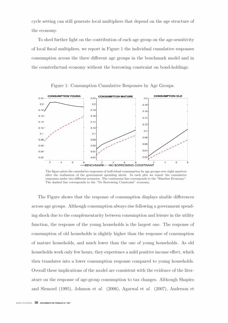
BANCO DE ESPAÑA 38 DOCUMENTO DE TRABAJO N.º 1837
cycle setting can still generate local multipliers that depend on the age structure of
the economy.
To shed further light on the contribution of each age group on the age-sensitivity
of local fiscal multipliers, we report in Figure 1 the individual cumulative responses
consumption across the three different age groups in the benchmark model and in
the counterfactual economy without the borrowing constraint on bond-holdings.
Figure 1: Consumption Cumulative Responses by Age Groups.
The figure plots the cumulative responses of individual consumption by age groups over eight quartersafter the realization of the government spending shock. In each plot we report the cumulativeresponses under two different scenarios. The continuous line corresponds to the “Baseline Economy”.The dashed line corresponds to the “No Borrowing Constraint” economy.
The Figure shows that the response of consumption displays sizable differences
across age groups. Although consumption always rise following a government spend-
ing shock due to the complementarity between consumption and leisure in the utility
function, the response of the young households is the largest one. The response of
consumption of old households is slightly higher than the response of consumption
of mature households, and much lower than the one of young households. As old
households work only few hours, they experience a mild positive income effect, which
then translates into a lower consumption response compared to young households.
Overall these implications of the model are consistent with the evidence of the liter-
ature on the response of age-group consumption to tax changes. Although Shapiro
and Slemord (1995), Johnson et al. (2006), Agarwal et al. (2007), Anderson et

BANCO DE ESPAÑA 39 DOCUMENTO DE TRABAJO N.º 1837
al. (2016) use different approaches to identify the consumption response to tax
shocks, they all conclude that young households display a much larger consumption
response than older individuals.26
The consumption response of young households is still larger than the response
of older individuals even when we eliminate the borrowing constraint. Indeed, in
our model the age-sensitivity of local fiscal multipliers hinges also on the market
incompleteness, that boosts the marginal propensity to consume of young agents.
The relevance of incomplete markets - above and beyond the fraction of borrowing
constrained agents - for the size of fiscal multipliers is also highlighted by Brinca et
al. (2016), Ferriere and Navarro (2017), and Hagedorn et al. (2017). In these papers,
markets are incomplete because the idiosyncratic labor income risk is uninsurable
and there is no state-contingent bonds. In our environment the lack of complete
markets is also rooted in the overlapping generation structure of the model. In
equilibrium, given the interest rate and the amount of bonds traded, young agents
cannot borrow sufficiently to smooth consumption in the face of a hump-shaped
labor income dynamics over the life-cycle.27 As a result, the marginal propensity to
consume of young households is above the one of mature households, as it is in the
data. Hence, an economy with relatively more young households features a stronger
demand channel.
26Also Kaplan and Violante (2010), Berger al. (2018), and Carroll et al. (2018) provide model-based evidencepointing out that the marginal propensity to consume is highest among young households. Young householdsdisplay a larger marginal propensity because they are more likely to be liquidity constrained, as documented inJappelli (1990), Kaplan et al. (2014), and Misra and Surico (2014).
27The inability to trade bonds/write contracts with the agents that are unborn prevents the (current) youngagents from accessing additional asset markets to perfectly smooth consumption.
4.2.2 Local Fiscal Multipliers: Extensions of the Model
We consider two extensions of the baseline model to test the robustness of the
implications on local fiscal multipliers of our economy.
In the first extension, we let the labor supply elasticity ν to vary exogenously
across age groups. In the empirically relevant case, young and old workers have a
higher labor supply elasticity than mature workers. These differences capture the
fact that in the data the hours worked by young and old households are much more

BANCO DE ESPAÑA 40 DOCUMENTO DE TRABAJO N.º 1837
volatile than the hours worked by mature households. In our economy, since the
preferences are of the GHH family, these differences in the labor supply generate
heterogeneity across age groups in the response of labor to military spending. We
set the labor supply elasticity of mature individuals to νm = 0.2, at the lower end of
the Frisch elasticity estimates and at the average of the Hicksian elasticity estimates
in Chetty et al. (2013), the labor supply elasticity of old individuals to νo = 0.75,
following the evidence of Rogerson and Wallenius (2013) on the retirement behavior
from full-work, and the labor supply elasticity of old individuals to νy = 0.71, such
as the weighted-average elasticity of the economy keeps being at 0.4.28
In the second extension, we split the young individuals in two groups: one group
faces a borrowing constraint on bond-holdings whereas the other group can freely
borrow. This feature allows us to calibrate the share of borrowing constrained
young individuals to the data, and therefore have a better understanding of the
28Our calibration choice for the labor supply elasticity across age groups is consistent with French (2005),Jaimovich and Siu (2009), Rogerson and Wallenius (2009), Erosa et al. (2016), Janiak and Monteiro (2016),Karabarbounis (2016), Peterman (2016), who find that young and old individuals have higher labor supplyelasticities than mature individuals. The differences across age groups in the labor supply elasticity are alsomotivated by the response of hours to a government spending shock in the data. In Appendix A.3, we computehours worked by state for all workers, young workers (workers between 20 and 29 years old), and older workers(workers above 30 years old) using CPS data from 1977 to 2015. When we estimate the hours worked local fiscalmultiplier, we find that total hours increase following a government spending shock. Since the sample startsonly in 1977, we lose the first ten years of our baseline sample, which implies that the uncertainty around thelocal multiplier estimates becomes rather large. Then, we compare the estimates of the local fiscal multiplierfor the hours worked by young and older workers. Although the large standard deviations make the estimatesnot to be statistically different from zero, the point estimate of the local multiplier for the hours worked by theyoung is 2.5 times larger than the point estimate of the local multiplier for the hours worked by the rest of thepopulation.
contribution of the ad-hoc borrowing constraint on the results of the model. We set
the ad-hoc borrowing constraint to be binding only for 40% of the young households,
which is the fraction of poor and wealthy hand-to-mouth households aged between
20 and 29 in the U.S., as computed by Kaplan et al. (2014).
Then, we replicate the exercise on the local fiscal multiplier with these two exten-
sions of the model, and compare the results in Table 6. Allowing for the responses
of labor to military spending to differ across age groups raises only slightly the age
sensitivity of local fiscal multipliers, from 2% to 2.2%. Also considering that the
borrowing constraint binds for only 40% of young individuals generates a limited
change in the age sensitivity of local fiscal multipliers, that goes to 1.7%.

BANCO DE ESPAÑA 41 DOCUMENTO DE TRABAJO N.º 1837
Table 6: Age Sensitivity of Local Output Fiscal Multiplier - Model Extensions
Data Baseline Age-Specific 40% YoungModel Labor Supply Borrowing
Elasticity Constrained
Δ Local Output Fiscal Multiplier of 3.1% 2% 2.2% 1.7%1% Increase in Share Young People
Note: The Table reports the results of the age sensitivity of local output fiscal multiplier in the data and in twoextensions of the “Baseline Model”: the “Age-Specific Labor Supply Elasticity” economy, in which the labor supplyelasticity varies exogenously across age-groups, and the “40% Young Borrowing Constrained”, in which the ad-hocconstraint binds only for 40% of young individuals.
4.2.3 Demographics and National Fiscal Multipliers
Does the link between demographics and fiscal multipliers persist also at the na-
tional level? Although our evidence shows that the effect of demographics on fiscal
multipliers at the state level is economically and statistically significant, this result
does not necessarily imply that demographics alter also national multipliers. Indeed,
Nakamura and Steinsson (2014), Fahri and Werning (2016), and Chodorow-Reich
(2018) show that local fiscal multipliers consider the local effect of federally financed
policies and wash out any monetary policy response to government spending. Both
features make local multipliers larger than national ones. On the other hand, local
multipliers are dampened by expenditure switching and import leakage effects that
do not take place at the national level.
We evaluate the role of the age structure on the size of national fiscal multipliers
through the lenses of the model. To do so, we estimate national multipliers in the
following exercise. First, we consider a symmetric increase in government spending
in both the home and the foreign economy. Similarly to our definition of national
output Y Ut , we define national government spending as sum of government spending
in the home economy and government spending in the foreign economy, that is, Gut =
GH,t +GF,t. Hence, now we consider an increase in national (wasteful) government
spending which is financed by all the individuals in the monetary union.
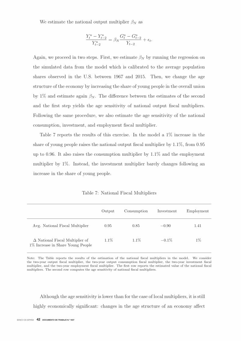
BANCO DE ESPAÑA 42 DOCUMENTO DE TRABAJO N.º 1837
We estimate the national output multiplier βN as
Y ut − Y u
t−2Y ut−2
= βN
Gut −Gu
t−2Yt−2
+ εt.
Again, we proceed in two steps. First, we estimate βN by running the regression on
the simulated data from the model which is calibrated to the average population
shares observed in the U.S. between 1967 and 2015. Then, we change the age
structure of the economy by increasing the share of young people in the overall union
by 1% and estimate again βN . The difference between the estimates of the second
and the first step yields the age sensitivity of national output fiscal multipliers.
Following the same procedure, we also estimate the age sensitivity of the national
consumption, investment, and employment fiscal multiplier.
Table 7 reports the results of this exercise. In the model a 1% increase in the
share of young people raises the national output fiscal multiplier by 1.1%, from 0.95
up to 0.96. It also raises the consumption multiplier by 1.1% and the employment
multiplier by 1%. Instead, the investment multiplier barely changes following an
increase in the share of young people.
Table 7: National Fiscal Multipliers
Output Consumption Investment Employment
Avg. National Fiscal Multiplier 0.95 0.85 −0.90 1.41
Δ National Fiscal Multiplier of 1.1% 1.1% −0.1% 1%1% Increase in Share Young People
Note: The Table reports the results of the estimation of the national fiscal multipliers in the model. We considerthe two-year output fiscal multiplier, the two-year output consumption fiscal multiplier, the two-year investment fiscalmultiplier, and the two-year employment fiscal multiplier. The first row reports the estimated value of the national fiscalmultipliers. The second row computes the age sensitivity of national fiscal multipliers.
Although the age sensitivity is lower than for the case of local multipliers, it is still
highly economically significant: changes in the age structure of an economy affect

BANCO DE ESPAÑA 43 DOCUMENTO DE TRABAJO N.º 1837
fiscal multipliers also at the national level. In Appendix B we validate the prediction
of the model on the link between demographics and national fiscal multipliers. We
estimate a SVAR on both a panel of developed countries and a panel of developing
countries and identify government spending shock with a Choleski ordering a la
Blanchard and Perotti (2002). In either case, we show that the long-run national
output fiscal multiplier is indeed larger in countries with higher shares of young
people in total population.

BANCO DE ESPAÑA 44 DOCUMENTO DE TRABAJO N.º 1837
5 Population Aging and Fiscal Multipliers
After the World War II, the demographic structure of the U.S. population has been
changing dramatically over time. For instance, the onset of the baby boomers raised
the share of young people by 22% between 1967 and 1980. From 1980 on, the U.S.
population has progressively shifted towards older ages. Indeed, from 1980 to 2015
the share of young people has shrunk by 30%.
What are the implications of the aging of the U.S. population on the effectiveness
of fiscal policy? We address this question by feeding the model with the entire path
of population shares observed from 1967 until 2015, and then compute national
fiscal multipliers through the lenses of the model.29 Figure 2 shows the results of
this exercise for the output fiscal multiplier.
The output fiscal multiplier was 0.97 in 1970 and increased up to 1.19 in 1980,
when the effect of the baby boom on the share of young people was the greatest.
As the share of young people progressively shrinks, the multiplier starts decreasing,
drops below 1 in 1990, and reaches a value of 0.76 in 2015. Hence, the model predicts
that over the last forty years the size of the output fiscal multipliers went down by
36%. Interestingly, even if we remove the ad-hoc borrowing constraint, the model
predicts that from 1980 to 2015 the national output fiscal multiplier has decreased
by 31%.
These results are consistent with the empirical evidence of Blanchard and Perotti
(2002), Bilbiie et al. (2008), and Pereira and Lopes (2014) on the reduction of the
size of U.S. fiscal multipliers over time.30 Both papers show that fiscal multipliers in
the recent decades are smaller than what they used to be during the 1960s and 1970s.
From this perspective, our model provides a rationale of this empirical finding, by
linking the process of aging of the U.S. population to the observed reduction in the
effectiveness of fiscal policy.
29In this exercise, we only change the age structure of the model to isolate the role of the demographictransition on the size of fiscal multipliers. All the other features of the model are kept constant, e.g., themonetary policy stance and the degree of credit market imperfections. Although in our model changes inthe demographic structure generate endogenous variation in the degree of credit market imperfections, weacknowledge that this patter captures only a fraction of process of financial development of U.S. credit markets.
30Kirchner et al. (2010), Cimadomo and D’Agostino (2016), Glocker et al. (2017) find also a drop in the sizeof multipliers in Germany, Italy and the United Kingdom.
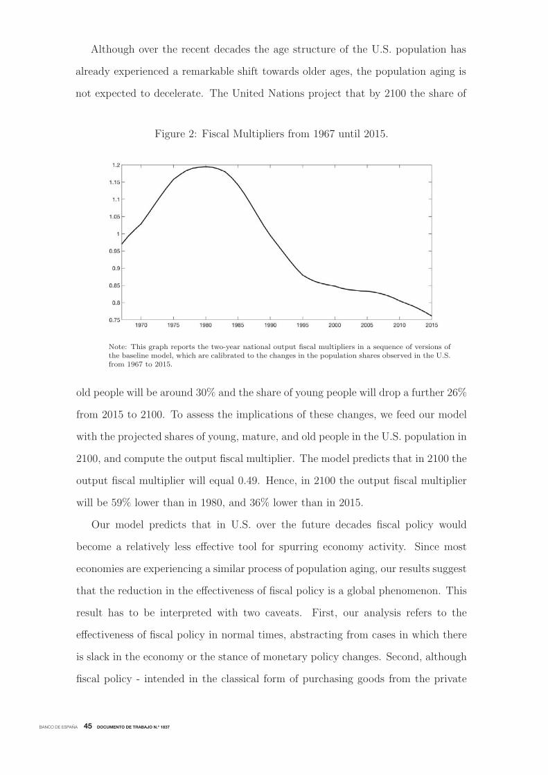
BANCO DE ESPAÑA 45 DOCUMENTO DE TRABAJO N.º 1837
Although over the recent decades the age structure of the U.S. population has
already experienced a remarkable shift towards older ages, the population aging is
not expected to decelerate. The United Nations project that by 2100 the share of
Figure 2: Fiscal Multipliers from 1967 until 2015.
Note: This graph reports the two-year national output fiscal multipliers in a sequence of versions ofthe baseline model, which are calibrated to the changes in the population shares observed in the U.S.from 1967 to 2015.
old people will be around 30% and the share of young people will drop a further 26%
from 2015 to 2100. To assess the implications of these changes, we feed our model
with the projected shares of young, mature, and old people in the U.S. population in
2100, and compute the output fiscal multiplier. The model predicts that in 2100 the
output fiscal multiplier will equal 0.49. Hence, in 2100 the output fiscal multiplier
will be 59% lower than in 1980, and 36% lower than in 2015.
Our model predicts that in U.S. over the future decades fiscal policy would
become a relatively less effective tool for spurring economy activity. Since most
economies are experiencing a similar process of population aging, our results suggest
that the reduction in the effectiveness of fiscal policy is a global phenomenon. This
result has to be interpreted with two caveats. First, our analysis refers to the
effectiveness of fiscal policy in normal times, abstracting from cases in which there
is slack in the economy or the stance of monetary policy changes. Second, although
fiscal policy - intended in the classical form of purchasing goods from the private

BANCO DE ESPAÑA 46 DOCUMENTO DE TRABAJO N.º 1837
sector - becomes less effective in spurring economic activity due to population aging,
fiscal interventions targeted to specific age groups could be still highly expansionary.
To this end, a new class of model as ours could be used as a laboratory to design
and evaluate the effects of such policies.

BANCO DE ESPAÑA 47 DOCUMENTO DE TRABAJO N.º 1837
6 Conclusion
This paper shows that the age structure of an economy determines the effectiveness
of fiscal policy such that fiscal multipliers are larger in economies with higher shares
of young people in total population.
First, we identify the causal effect of a change in demographics on the size of
fiscal multipliers using the variation across U.S. states in government spending and
lagged birth rates. We find that a 1% increase in the share of people between 20
and 29 years in total population raises the local fiscal multipliers by 3.1%.
Second, to rationalize this finding we build a tractable life-cycle open-economy
New Keynesian model with two forms of credit market imperfections: incomplete
asset markets and an ad-hoc borrowing constraint. The model can explain 65%
of the link between demographics and local fiscal multipliers: in the model a 1%
increase in the share of people between 20 and 29 years in total population raises
the local fiscal multipliers by 2%. Demographics affect the size of fiscal multipliers
also at the national level. Indeed, a 1% increase in the share of young people raises
the national fiscal multipliers by 1.1%.
Third, we use the model to study the implications of population aging for the
effectiveness of fiscal policy. Over the recent decades, the demographic structure of
the U.S. population has progressively shifted towards older ages: the share of young
people in total population plummeted by 30% from 1980 to 2015. Once we feed
this shift in population shares into our model, we find that nowadays national fiscal
multipliers are 36% lower than forty years ago. This result suggests that the process
of population aging could dampen over time the effectiveness of fiscal policy.
BANCO DE ESPAÑA 48 DOCUMENTO DE TRABAJO N.º 1837
References
Agarwal, S., C. Liu, and N. Souleles. 2007. The Reaction of Consumer Spend-
ing and Debt to Tax Rebates - Evidence from Consumer Credit Data. Journal of
Political Economy, 115, 986-1019.
Aksoy, Y., H. S. Basso, R. Smith, and T. Grasl. 2018. Demographic Struc-
ture and Macroeconomic Trends. American Economic Journal: Macroeconomics,
forthcoming.
Anderson, E., A. Inoue, and B. Rossi. 2016. Heterogeneous Consumers and
Fiscal Policy Shocks. Journal of Money Credit and Banking, 48, 1877-88.
Auerbach, A., and Y. Gorodnichenko. 2012. Measuring the Output Responses
to Fiscal Policy. American Economic Journal: Economic Policy, 4, 1-27.
Barro, R. 1981. Output Effects of Government Purchases. Journal of Political
Economy, 89, 1086-121.
Barro, R., and C. Redlick. 2011. Macroeconomic Effects from Government
Purchases and Taxes. Quarterly Journal of Economics, 126, 51-102.
Berger, D., V. Guerrieri, G. Lorenzoni, and J. Vavra. 2018. House Prices
and Consumer Spending. Review of Economic Studies, 85, 1502-42.
Bilbiie, F. 2011. Nonseparable Preferences, Frisch Labor Supply, and the Con-
sumption Multiplier of Government Spending: One Solution to a Fiscal Policy Puz-
zle. Journal of Money, Credit, and Banking, 43, 221-51.
Bilbiie, F., G. Mueller, and A. Meier. 2008. What Accounts for the Change
in U.S. Fiscal Policy Transmission? Journal of Money, Credit and Banking, 40,
1439-70.
Blanchard, O. 1985. Debt, Deficits, and Finite Horizons. Journal of Political
Economy, 93, 223-47.
Blanchard, O., and L. Katz. 1992 Regional Evolutions. Brookings Papers on
Economic Activity, 1, 1-75.
Blanchard, O., and R. Perotti. 2002. An Empirical Characterization of the
Dynamic Effects of Changes in Government Spending and Taxes on Output. Quar-
terly Journal of Economics, 117, 1329-68.

BANCO DE ESPAÑA 49 DOCUMENTO DE TRABAJO N.º 1837
Bouakez, H., O. Rachedi, and E. Santoro. 2018. Sectoral Heterogeneity, Pro-
duction Networks, and the Effects of Government Spending. Mimeo.
Brinca, P., Holter, H., Krusell, P., and L. Malafry. 2016. Fiscal Multipliers
in the 21st Century. Journal of Monetary Economics, 77, 53-69.
Calvo, G. 1983. Staggered Prices in a Utility-Maximizing Framework. Journal of
Monetary Economics, 12, 383-98.
Carroll, C., J. Slacalek, K. Tokuoka, and M. White. 2017. The Distribution
of Wealth and the Marginal Propensity to Consume. Quantitative Economics, 8,
977-1020.
Carvalho, C., A. Ferrero, and F. Nechio. 2016. Demographics and Real In-
terest Rates: Inspecting the Mechanism. European Economic Review, 88, 208-26.
Chetty, R., A. Guren, D. Manoli, and A. Weber. 2013. Does Indivisible La-
bor Explain the Difference Between Micro and Macro Elasticities? A Meta-Analysis
of Extensive Margin Elasticities. NBER Macroeconomics Annual, 27, 1-56.
Christiano, L., M. Eichenbaum, and S. Rebelo. 2011. When Is the Govern-
ment Spending Multiplier Large? Journal of Political Economy, 119, 78-121.
Chodorow-Reich, G. 2018. Geographic Cross-Sectional Fiscal Multipliers: What
Have We Learned? American Economic Journal: Economic Policy, forthcoming.
Cimadomo, J., and A. D’Agostino. 2016. Combining Time Variation and
Mixed Frequencies: an Analysis of Government Spending Multipliers in Italy. Jour-
nal of Applied Econometrics, 31, 1276-90.
Clarida, R., J. Gali, and M. Gertler. 2000. Monetary Policy Rules and Macroe-
conomic Stability: Evidence and Some Theory. Quarterly Journal of Economics,
115, 147-80.
Constantinides, G., J. Donaldson, and R. Mehra. 2002. Junior Can’t Bor-
row: A New Perspective on the Equity Premium Puzzle. Quarterly Journal of
Economics, 117, 269-96.
Epstein, L., and S. Zin. 1989. Substitution, Risk Aversion, and the Temporal
Behavior of Consumption and Asset Returns: A Theoretical Framework. Econo-
metrica, 57, 937-69.
BANCO DE ESPAÑA 50 DOCUMENTO DE TRABAJO N.º 1837
Erosa, A., Fuster, L., and G. Kambourov. 2016. Towards a Micro-Founded
Theory of Aggregate Labour Supply. Review of Economic Studies, 83, 1001-39.
Farhi, E., and I. Werning. 2016. Fiscal Multipliers: Liquidity Traps and Cur-
rency Unions. Handbook of Macroeconomics, 2, 2417-92.
Ferraro, D., and G. Fiori. 2017. Aging of the Baby Boomers: Demographics
and Propagation of Tax Shocks. Mimeo.
Ferriere, X., and G. Navarro. 2017. The Heterogeneous Effects of Government
Spending: It’s All About Taxes. Mimeo.
French, E. 2005. The Effects of Health, Wealth, and Wages on Labor Supply and
Retirement Behavior. Review of Economic Studies, 72, 395-427.
Gali, J., D. Lopez-Salido, and J. Valles. 2007. Understanding the Effects of
Government Spending on Consumption. Journal of the European Economic Asso-
ciation, 5, 227-70.
Gertler, M. 1999. Government Debt and Social Security in a Life-Cycle Economy.
Carnegie-Rochester Conference Series on Public Policy, 50, 61-110.
Glocker, C., G. Sestrieri, and P. Towbin. 2017. Time-Varying Fiscal Spending
Multipliers in the UK. Mimeo.
Gnocchi, S., D. Hauser, and E. Pappa. 2016. Housework and Fiscal Expan-
sions. Journal of Monetary Economics, 79, 94-108.
Gordon, R., and H. Varian. 1988. Intergenerational Risk Sharing. Journal of
Public Economics, 37, 185-202.
Hagedorn, M., I. Manovskii, and K. Mitman. 2017. The Fiscal Multiplier.
Mimeo.
Hall, R. 1988. Intertemporal Substitution in Consumption. Journal of Political
Economy, 96, 339-57.
Hall, R. 2009. By How Much Does GDP Rise If the Government Buys More Out-
put? Brookings Papers on Economic Activity, 2, 183-231.
Ilzetzki, E., E. Mendoza, and C. Vegh. 2013. How Big (Small?) Are Fiscal
Multipliers? Journal of Monetary Economics, 60, 239-54.

BANCO DE ESPAÑA 51 DOCUMENTO DE TRABAJO N.º 1837
Jaimovich, N., and H. Siu. 2009. The Young, the Old, and the Restless: De-
mographics and Business Cycle Volatility. American Economic Review, 99, 804-26.
Janiak, A., and P. Santos Monteiro. 2016. Towards a Quantitative Theory
of Automatic Stabilizers: The Role of Demographics. Journal of Monetary Eco-
nomics, 78, 35-49.
Jappelli, T. 1990. Who is Credit Constrained in the U.S. Economy? Quarterly
Journal of Economics, 105, 219-34.
Johnson, D., J. Parker, and N. Soulele. 2006. Household Expenditure and
the Income Tax Rebates of 2001. American Economic Review, 96, 1589-610.
Kaplan, G., G. Violante, and J. Weidner. 2014. The Wealthy Hand-to-Mouth.
Brookings Papers on Economic Activity, 77-138.
Kaplan, G., and G. Violante. 2010. How Much Consumption Insurance Beyond
Self-Insurance? American Economic Journal: Macroeconomics, 2, 53-87.
Kaplan, G., and G. Violante. 2016. A Model of the Consumption Response to
Fiscal Stimulus Payments. Econometrica, 82, 1199-239.
Karabarbounis, M. 2016. A Roadmap for Efficiently Taxing Heterogeneous
Agents. American Economic Journal: Macroeconomics, 8, 182-214.
Kirchner, M., J. Cimadomo, and S. Hauptmeier. 2010 Transmission of Gov-
ernment Spending Shocks in the Euro Area: Time Variation and Driving Forces.
Mimeo.
Kormilitsina, A., and S. Zubairy. 2018. Propagation Mechanisms for Gov-
ernment Spending Shocks: A Bayesian Comparison. Journal of Money, Credit and
Banking, forthcoming.
Krueger, D., and A. Ludwig. 2007. On the Consequences of Demographic
Change for Rates of Returns to Capital, and the Distribution of Wealth and Wel-
fare. Journal of Monetary Economics, 54, 49-87.
Leeper, E., N. Traum, and T. Walker. 2017. Clearing Up the Fiscal Multiplier
Morass. American Economic Review, 107, 2409-54.
BANCO DE ESPAÑA 52 DOCUMENTO DE TRABAJO N.º 1837
Misra, K., and P. Surico. 2014. Consumption, Income Changes, and Heterogene-
ity: Evidence from Two Fiscal Stimulus Programs. American Economic Journal:
Macroeconomics, 6, 84-106.
Nakamura, E., and J. Steinsson. 2014. Fiscal Stimulus in a Monetary Union:
Evidence from US Regions. American Economic Review, 104, 753-92.
Oh, H., and R. Reis. 2012. Targeted Transfers and the Fiscal Response to the
Great Recession. Journal of Monetary Economics, 59, 50-64.
Pereira, M., and A. Lopes. 2014. Time-Varying Fiscal Policy in the US. Studies
in Nonlinear Dynamics & Econometrics, 18, 157-184.
Peterman, W. 2016. Reconciling Micro and Macro Estimates of the Frisch Labor
Supply Elasticity. Economic Inquiry, 54, 100-20.
Ramey, V. 2011. Identifying Government Spending Shocks: It’s All in the Timing.
Quarterly Journal of Economics, 126, 1-50.
Ramey, V., and S. Zubairy. 2018. Government Spending Multipliers in Good
Times and in Bad: Evidence from U.S. Historical Data. Journal of Political Econ-
omy, 126, 850-901.
Rendahl, P. 2016. Fiscal Policy in an Unemployment Crisis. Review of Economic
Studies, 83, 1189-224.
Rogerson, R., and J. Wallenius. 2013. Nonconvexities, Retirement and the
Elasticity of Labor Supply. American Economic Review, 103, 1445-62.
Romer, C., and D. Romer. 2010. The Macroeconomic Effects of Tax Changes:
Estimates Based on a New Measure of Fiscal Shocks. American Economic Review,
100, 763-801.
Shapiro, M., and J. Slemrod. 1995. Consumer Response to the Timing of In-
come: Evidence from a Change in Tax With-holding. American Economic Review,
85, 274-83.
Shimer, R. 2001. The Impact of Young Workers on the Aggregate Labor Market.
Quarterly Journal of Economics, 116, 969-1007.
BANCO DE ESPAÑA 53 DOCUMENTO DE TRABAJO N.º 1837
Sims, E., and J. Wolff. 2018. The Output and Welfare Effects of Government
Spending Shocks over the Business Cycle. International Economic Review, forth-
coming.
Suarez Serrato, J., and P. Wingender. 2016. Estimating Local Fiscal Multi-
pliers. Mimeo.
Wong, A. 2016. Population Aging and the Transmission of Monetary Policy to
Consumption. Mimeo.
Woodford, M. 2011. Simple Analytics of the Government Expenditure Multiplier.
American Economic Journal: Macroeconomics, 3, 1-35.
Yaari, M. 1965. Uncertain Lifetime, Life Insurance, and the Theory of the Con-
sumer. Review of Economic Studies, 32, 137-50.

BANCO DE ESPAÑA 54 DOCUMENTO DE TRABAJO N.º 1837
A Local Fiscal Multipliers: Further Evidence
A.1 Additional State-Level Controls
The estimates of the age sensitivity of local fiscal multipliers in the baseline regres-
sions could be biased in case the exclusion restrictions of our IV approach is vio-
lated, which would happen in case there exist potential confounding factors which
are highly correlated with both changes (across states and over time) in the currant
age structure of the population, changes (across states and over time) in 20-30 year
lagged birth rates, and changes (across states and over time) in current government
spending.
This Section addresses this issue by reporting a comprehensive battery of ro-
bustness checks, in which we explicitly control for the same set of state-level key
variables introduced in Section 2.4: per capita real federal personal taxes (provided
by the BEA), the unemployment rate (provided from the BLS from 1976 on), the
ratio of unemployment benefits over personal income (provided from the BLS from
1976 on), the Gini index of labor earnings (derived from labor earnings across indi-
viduals in CPS data from 1977 on), a measure of skilled labor (derived from CPS
data from 1977 on), a measure of female labor participation (derived from CPS
data from 1977 on), the share of services in value added (provided by the BEA),
the share of personal services in value added (provided by the BEA), and the share
of health care services in value added (provided by the BEA).
Table A.1 shows the estimate of the output fiscal multiplier, whereas Table A.2
reports a similar battery of robustness checks for the employment fiscal multiplier.
In all cases the estimated coefficient on the interaction between state government
spending and the log-share of young people is always highly statistically and eco-
nomically significant. Actually, the introduction of additional controls alters the
level of fiscal multipliers but not the sensitivity of multipliers to states’ age struc-
ture.

BANCO DE ESPAÑA 55 DOCUMENTO DE TRABAJO N.º 1837
Table A.1: Response of Output to a Government Shock - Additional State-Level Variables
(1) (2) (3) (4) (5) (6) (7) (8) (9)
Personal Unempl. Unempl. Gini Skilled Female Labor Services Personal Health CareTaxes Rate Benefits Earnings Labor Participation Share Services Services
Share Share
IV IV IV IV IV IV IV IV IV
Gi,t−Gi,t−2
Yi,t−21.506��� 0.581 1.434��� 1.232��� 1.080�� 1.0177�� 1.252��� 1.510��� 1.041��
(0.409) (0.407) (0.390) (0.477) (0.453) (0.478) (0.368) (0.407) (0.408)
Gi,t−Gi,t−2
Yi,t−2× 0.049��� 0.041��� 0.049��� 0.069��� 0.077��� 0.072��� 0.053��� 0.061��� 0.034��
(Di,t − D
)(0.018) (0.016) (0.017) (0.017) (0.022) (0.018) (0.018) (0.021) (0.016)
Gi,t−Gi,t−2
Yi,t−2× -0.043 0.254 -0.069 9.203 4.097 18.649 -4.787 -18.361 -34.473
(V ARi,t − V AR
)(0.043) (0.270) (0.042) (14.738) (5.450) (18.969) (2.986) (23.774) (21.193)
Di,t 0.001��� 0.001�� 0.001��� 0.001�� 0.001� 0.001� 0.001�� 0.001��� 0.001��
(0.001) (0.001) (0.001) (0.001) (0.001) (0.001) (0.001) (0.001) (0.001)
R2 0.369 0.452 0.363 0.348 0.353 0.350 0.370 0.365 0.368
N. Obs. 2374 2031 2374 1982 1982 1982 2374 2374 2374
Note: The table reports the estimates of panel regressions across U.S. states using data from 1967 to 2015 at an annual frequency, in which the dependent variableis the change in per capita real output. In all regressions, the independent variables are the change in per capita government spending, (Gi,t −Gi,t−2) /Yi,t−2, thelog-share of young people (aged 20-29) in total population, Di,t, and the interaction between the change in per capita government spending and the share of youngpeople, [(Gi,t −Gi,t−2) /Yi,t−2]×
(Di,t − D
). State-specific changes in state per capita government spending (as a fraction of state per capita GDP) are instrumented
with the product of state fixed effects and the change in national per capita government spending (as a fraction of national per capita GDP). The share of youngpeople is instrumented with 20-30 year lagged birth rates. In regressions (1) - (5) we include one additional national-level control to the benchmark specification, whichwe interact with state-fixed effects. Regression (1) includes the log-difference of the real oil price. Regression (2) includes households’ debt to GDP ratio. Regression(3) includes federal debt to GDP ratio. Regression (4) includes the level of the real interest rate. Regression (5) includes Ramey government spending news variable.In regressions (6) - (9) we include one additional state-level control to the benchmark specification. Regression (6) includes the log-difference of the real house price.Regression (7) includes per capita real households’ federal taxes. Regression (8) includes the unemployment rate. Regression (9) includes per capita real unemploymentbenefits. Robust standard errors clustered at the state level are reported in brackets. ∗, ∗∗, and ∗∗∗ indicate statistical significance at the 10%, 5% and 1%, respectively.

BANCO DE ESPAÑA 56 DOCUMENTO DE TRABAJO N.º 1837
Table A.2: Response of Employment Rate - Additional State-Level Variables
(1) (2) (3) (4) (5) (6) (7) (8) (9)
Personal Unempl. Unempl. Gini Skilled Female Labor Services Personal Health CareTaxes Rate Benefits Earnings Labor Participation Share Services Services
Share Share
IV IV IV IV IV IV IV IV IV
Gi,t−Gi,t−2
Yi,t−21.093��� 0.351 1.060��� 0.629�� 0.507� 0.608�� 1.076��� 1.057��� 1.001���
(0.218) (0.228) (0.198) (0.291) (0.294) (0.293) (0.190) (0.219) (0.239)
Gi,t−Gi,t−2
Yi,t−2× 0.035��� 0.040��� 0.036��� 0.043��� 0.049��� 0.047��� 0.031��� 0.039��� 0.032��
(Di,t − D
)(0.011) (0.010) (0.010) (0.012) (0.011) (0.011) (0.011) (0.014) (0.013)
Gi,t−Gi,t−2
Yi,t−2× -0.012 -0.154 -0.028 25.739��� 2.871 23.428� 0.683 -13.601 -7.784
(V ARi,t − V AR
)(0.027) (0.134) (0.020) (9.987) (2.094) (11.631) (1.036) (12.636) (10.846)
Di,t 0.001 -0.001� 0.001 -0.001 -0.001� -0.001� 0.001 0.001 0.001(0.001) (0.001) (0.001) (0.001) (0.001) (0.001) (0.001) (0.001) (0.001)
R2 0.618 0.720 0.614 0.655 0.670 0.661 0.633 0.614 0.621
N. Obs. 2374 2031 2374 1982 1982 1982 2374 2374 2374
Note: The table reports the estimates of panel regressions across U.S. states from 1967 to 2015, at an annual frequency, in which the dependent variable is thechange in employment rate. In all regressions, the independent variables are the change in per capita government spending, (Gi,t −Gi,t−2) /Yi,t−2, the share ofyoung people (aged 20-29) in total population, Di,t, and the interaction between the change in per capita government spending and the log-share of young people,[(Gi,t −Gi,t−2) /Yi,t−2] ×
(Di,t − D
). State-specific changes in state per capita government spending (as a fraction of state per capita GDP) are instrumented with
the product of state fixed effects and the change in national per capita government spending (as a fraction of national per capita GDP). The share of young peopleis instrumented with 20-30 year lagged birth rates. In regressions (1) - (5) we include one additional national-level control to the benchmark specification, which weinteract with state-fixed effects. Regression (1) includes the log-difference of the real oil price. Regression (2) includes households’ debt to GDP ratio. Regression(3) includes federal debt to GDP ratio. Regression (4) includes the level of the real interest rate. Regression (5) includes Ramey government spending news variable.In regressions (6) - (9) we include one additional state-level control to the benchmark specification. Regression (6) includes the log-difference of the real house price.Regression (7) includes per capita real households’ federal taxes. Regression (8) includes the unemployment rate. Regression (9) includes per capita real unemploymentbenefits. Robust standard errors clustered at the state level are reported in brackets. ∗, ∗∗, and ∗∗∗ indicate statistical significance at the 10%, 5% and 1%, respectively.

BANCO DE ESPAÑA 57 DOCUMENTO DE TRABAJO N.º 1837
A.2 Additional National-Level Controls
In the baseline regressions we control for time fixed effects, which wash out the effects
of national-level factor. Yet, if states differ in the responsiveness to national-level
factors, and this heterogeneity correlates with the age structure of the population,
then our estimates of the age sensitivity of local fiscal multipliers could be biased.
This Section addresses this point by running a battery of regressions in which
each time we control for the interaction between a key national-level variable and
state fixed effects, so that the regressions control for states’ heterogeneous respon-
siveness to these national-level variables. Namely, as national-level variables we
consider the oil price (the annual average spot price of West Texas Intermediate),
households’ debt to GDP (the ratio of the credit market instruments - liability -
of the households and nonprofit organizations from the Financial Accounts of the
U.S. over the series of national GDP provided by the BEA), federal debt to GDP
(the ratio of the total public debt from the U.S. Office of Management and Budget
over the series of national GDP provided by the BEA), the military news variable
of Ramey (2011) and Ramey and Zubairy (2018), and the real interest rate (the
difference between the effective federal funds rate from the St. Louis Federal Re-
serves FRED database and the change in the Consumer Price Index for all urban
consumers from the BLS).
Table A.3 reports the results of the regressions in which the dependent vari-
able is the change in real per capita output whereas in Table A.4 the dependent
variable is the employment rate. In all cases, the age sensitivity of local fiscal mul-
tipliers is always highly statistically significant, and again roughly constant across
specifications.

BANCO DE ESPAÑA 58 DOCUMENTO DE TRABAJO N.º 1837
Table A.3: Response of Output with Additional National-Level Variables
(1) (2) (3) (4) (5)
Oil Households’ Federal Real Interest RameyPrice Debt Debt Rate News
IV IV IV IV IV
Gi,t−Gi,t−2
Yi,t−21.311∗∗∗ 1.661∗∗∗ 1.511∗∗∗ 1.500∗∗∗ 1.508∗∗∗
(0.333) (0.451) (0.443) (0.395) (0.416)
Gi,t−Gi,t−2
Yi,t−2× 0.039∗∗ 0.065∗∗∗ 0.041∗∗ 0.048∗∗∗ 0.039∗∗
(Di,t − D
)(0.015) (0.022) (0.017) (0.017) (0.018)
Di,t 0.001∗∗ 0.002∗∗ 0.002∗∗∗ 0.001∗∗ 0.002∗∗∗
(0.001) (0.001) (0.001) (0.001) (0.001)
R2 0.446 0.371 0.397 0.405 0.389
N. Obs. 2374 2374 2374 2374 2374
Note: The table reports the estimates of panel regressions across U.S. states using data from 1967 to2015 at an annual frequency, in which the dependent variable is the change in per capita real output.In all regressions, the independent variables are the change in per capita government spending,(Gi,t −Gi,t−2) /Yi,t−2, the log-share of young people (aged 20-29) in total population, Di,t, andthe interaction between the change in per capita government spending and the share of young people,[(Gi,t −Gi,t−2) /Yi,t−2]×
(Di,t − D
). State-specific changes in state per capita government spending
(as a fraction of state per capita GDP) are instrumented with the product of state fixed effects andthe change in national per capita government spending (as a fraction of national per capita GDP).The share of young people is instrumented with 20-30 year lagged birth rates. All regressions includeone additional national-level control to the benchmark specification, which we interact with state-fixed effects. Regression (1) includes the log-difference of the real oil price. Regression (2) includeshouseholds’ debt to GDP ratio. Regression (3) includes federal debt to GDP ratio. Regression (4)includes the level of the real interest rate. Regression (5) includes Ramey government spending newsvariable. Robust standard errors clustered at the state level are reported in brackets. ∗, ∗∗, and ∗∗∗indicate statistical significance at the 10%, 5% and 1%, respectively.

BANCO DE ESPAÑA 59 DOCUMENTO DE TRABAJO N.º 1837
Table A.4: Response of Employment Rate with Additional National-Level Variables
(1) (2) (3) (4) (5)
Oil Households’ Federal Real Interest RameyPrice Debt Debt Rate News
IV IV IV IV IV
Gi,t−Gi,t−2
Yi,t−21.104∗∗∗ 1.070∗∗∗ 1.025∗∗∗ 1.069∗∗∗ 1.073∗∗∗
(0.207) (0.013) (0.216) (0.211) (0.222)
Gi,t−Gi,t−2
Yi,t−2× 0.033∗∗∗ 0.040∗∗∗ 0.034∗∗∗ 0.032∗∗∗ 0.035∗∗∗
(Di,t − D
)(0.011) (0.013) (0.011) (0.011) (0.011)
Di,t 0.001 0.001 0.001 0.001 0.001(0.001) (0.001) (0.001) (0.001) (0.001)
R2 0.630 0.635 0.641 0.639 0.625
N. Obs. 2374 2374 2374 2374 2374
Note: The table reports the estimates of panel regressions across U.S. states from 1967 to 2015,at an annual frequency, in which the dependent variable is the change in employment rate. Inall regressions, the independent variables are the change in per capita government spending,(Gi,t −Gi,t−2) /Yi,t−2, the share of young people (aged 20-29) in total population, Di,t, and theinteraction between the change in per capita government spending and the log-share of young peo-ple, [(Gi,t −Gi,t−2) /Yi,t−2] ×
(Di,t − D
). State-specific changes in state per capita government
spending (as a fraction of state per capita GDP) are instrumented with the product of state fixedeffects and the change in national per capita government spending (as a fraction of national percapita GDP). The share of young people is instrumented with 20-30 year lagged birth rates. Allregressions include one additional national-level control to the benchmark specification, which weinteract with state-fixed effects. Regression (1) includes the log-difference of the real oil price. Re-gression (2) includes households’ debt to GDP ratio. Regression (3) includes federal debt to GDPratio. Regression (4) includes the level of the real interest rate. Regression (5) includes Rameygovernment spending news variable. Robust standard errors clustered at the state level are reportedin brackets. ∗, ∗∗, and ∗∗∗ indicate statistical significance at the 10%, 5% and 1%, respectively.

BANCO DE ESPAÑA 60 DOCUMENTO DE TRABAJO N.º 1837
A.3 Population Response to Government Spending Shocks
Table A.5 studies the response of state population to a government spending shock.
In this case, we estimate a simplified regression in which we consider as independent
variable just the change in state government spending:
Popi,t − Popi,t−2Popi,t−2
= αi + δt + βGi,t −Gi,t−2
Yi,t−2+ εi,t
where Popi,t denotes the population of state i at time t. In particular, we consider
four different definitions of population: (i) overall population, (ii) young popula-
tion (i.e., people between 20 and 29 years old), (iii) mature population (i.e., people
between 30 and 64 years old), and (iv) old population (i.e., people above 65 years
old). Given data availability on the disaggregation of total population across age
groups, this set of regressions uses annual data from 1969 until 2015.
Table A.5: Response of Population to a Government Spending Shock Across U.S. States
(1) (2) (3) (4)
Overall Population Young Population Mature Population Old Population
IV IV IV IV
Gi,t−Gi,t−2
Yi,t−2-0.179 1.145∗∗∗ -0.398 -0.070
(0.303) (0.399) (0.403) (0.212)
R2 0.611 0.654 0.584 0.790
N. Observations 2295 2295 2295 2295
Note: The table reports the estimates of panel regressions across U.S. states from 1969 to 2015 at an annual frequency.In Column (1) the dependent variable is the state overall white male population. In Column (2) the dependent variableis the state white male young population (aged 20-29). In Column (3) the dependent variable is the state white malemature population (aged 30-64). In Column (4) the dependent variable is the state white male old population (aged65+). The independent variable is the change in per capita state government spending (as a fraction of per capita stateGDP), which is instrumented with the product of state fixed effects and the change in per capita national governmentspending (as a fraction of per capita national GDP). We include time and state fixed effects in all the regressions.Robust standard errors clustered at the state level are reported in brackets. ∗, ∗∗, and ∗∗∗ indicate statistical significanceat the 10%, 5% and 1%, respectively.
Column (1) of Table A.5 shows that the overall population does not change fol-
lowing a government spending shock. Yet, this aggregate result compounds different

BANCO DE ESPAÑA 61 DOCUMENTO DE TRABAJO N.º 1837
dynamics of the populations by age group. On the one hand, column (2) shows that
the young population does rise following a fiscal shock. On the other hand, columns
(3) and (4) show that mature and old population shrink following a government
spending shock, even though this effect is not statistically significant.
These results are consistent with the findings of the literature on the sensitivity
of state population to shocks. On the one hand, Blanchard and Katz (1992) show
that state migration flows are important transmission mechanisms of changes in
state unemployment rates over time. On the other hand, Nakamura and Steinsson
(2014) find that overall state population does not react to government spending
shocks at short horizon. Our results emphasize that although overall population
may not change following a fiscal shock, this aggregate pattern masks heterogenous
reactions in the population of different age groups.
This evidence validates our approach in instrumenting the share of young people
with lagged birth rates. Indeed, as the young population does react to fiscal shocks,
using raw log-shares of the young people in total population would also capture
the endogenous reaction of states’ age structure to government spending shocks.
Hence, instrumenting the log-share of young people with lagged birth rates is key
to identify the causal effect of demographics on the size of fiscal multipliers.
A.4 Hours Worked Response to Government Spending Shocks
In the model we assume that the labor supply elasticity varies exogenously across
age groups. In the calibration exercise, the labor supply elasticity of young and old
individuals to be larger than the labor supply elasticity of mature individuals. This
feature reflects the fact that hours worked by young and old workers are much more
volatile than hours worked by mature workers.
In this Section, we show that our calibration choice is also consistent with the
response of hours worked to a government spending shock in the data. To do so,
we use CPS data to build a measure by state of hours worked by all workers, hours
worked by young workers (i.e., workers between 20 and 29 years old), and hours
worked by older workers (i.e., workers above 30 years old). Our measure of hours
BANCO DE ESPAÑA 62 DOCUMENTO DE TRABAJO N.º 1837
worked equals the per-worker amount of hours worked, in which we focus only on
non self-employed workers that are employed in the private sector.
Then, we use all these measures to estimate the effect of government spending on
state hours worked with a regression in which the dependent variable is the growth
rate of state hours worked Ni,t:
Ni,t −Ni,t−2Ni,t−2
= αi + δt + βGi,t −Gi,t−2
Yi,t−2+ εi,t (1)
Again, we instrument state military spending with a first-stage regression in which
the independent variable is the product of a state fixed effect and the change in
national military spending. Since CPS data start in 1977, we are left with 1887
observations, which is a substantial reduction in the sample size with respect our
benchmark analysis, that spans from 1967 to 2015.
Column (1) of Table A.6 shows that hours worked increase following a gov-
ernment spending shock. When we consider the disaggregated measures of hours
worked by young and older workers, the uncertainty around the estimates is so large
that we cannot reject the hypothesis that the local multiplier is zero in either case.
Nevertheless, the point estimates of Column (2) and (3) highlight that the hours
worked by young and older workers increase following a government spending shock,
but with different sensitivities. Indeed, the point estimate of the response of hours
worked by young workers is 2.5 times larger than the point estimate of the response
of hours worked by older workers. Although we do acknowledge that these estimates
are surrounded by a high degree of uncertainty, these results - together with the
findings of Jaimovich and Siu (2009) - are consistent with our modeling approach of
having the labor supply elasticity of young individuals to be higher than the labor
supply elasticity of older workers.
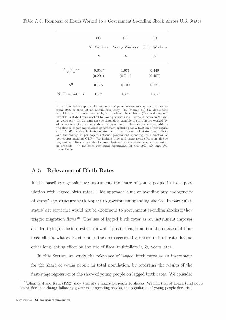
BANCO DE ESPAÑA 63 DOCUMENTO DE TRABAJO N.º 1837
Table A.6: Response of Hours Worked to a Government Spending Shock Across U.S. States
(1) (2) (3)
All Workers Young Workers Older Workers
IV IV IV
Gi,t−Gi,t−2
Yi,t−20.656∗∗ 1.036 0.449
(0.294) (0.711) (0.407)
R2 0.176 0.100 0.121
N. Observations 1887 1887 1887
Note: The table reports the estimates of panel regressions across U.S. statesfrom 1969 to 2015 at an annual frequency. In Column (1) the dependentvariable is state hours worked by all workers. In Column (2) the dependentvariable is state hours worked by young workers (i.e., workers between 20 and29 years old). In Column (3) the dependent variable is state hours worked byolder workers (i.e., workers above 30 years old). The independent variable isthe change in per capita state government spending (as a fraction of per capitastate GDP), which is instrumented with the product of state fixed effectsand the change in per capita national government spending (as a fraction ofper capita national GDP). We include time and state fixed effects in all theregressions. Robust standard errors clustered at the state level are reportedin brackets. ∗∗ indicates statistical significance at the 10%, 5% and 1%,respectively.
A.5 Relevance of Birth Rates
In the baseline regression we instrument the share of young people in total pop-
ulation with lagged birth rates. This approach aims at avoiding any endogeneity
of states’ age structure with respect to government spending shocks. In particular,
states’ age structure would not be exogenous to government spending shocks if they
trigger migration flows.31 The use of lagged birth rates as an instrument imposes
31Blanchard and Katz (1992) show that state migration reacts to shocks. We find that although total popu-lation does not change following government spending shocks, the population of young people does rise.
an identifying exclusion restriction which posits that, conditional on state and time
fixed effects, whatever determines the cross-sectional variation in birth rates has no
other long lasting effect on the size of fiscal multipliers 20-30 years later.
In this Section we study the relevance of lagged birth rates as an instrument
for the share of young people in total population, by reporting the results of the
first-stage regression of the share of young people on lagged birth rates. We consider

BANCO DE ESPAÑA 64 DOCUMENTO DE TRABAJO N.º 1837
four different cases for the share of young white males, the share of young males,
and the share of overall young people: (i) we regress the raw share of young people
on the raw series of lagged birth rates and both time and state fixed effects; (ii) we
regress the residual series of the raw share of young people on the residual series
of the raw series of lagged birth rates. Each residual variable is derived by taking
the residuals of a regression in which the dependent variable is is either the share
of young people or the lagged birth rates and the independent variables are state
and time fixed effects; (iii) we regress the log-share of young people on the series of
lagged birth rates in logarithm and both time and state fixed effects; (iv) we regress
the residual series of the log-share of young people on the residual series of the series
of lagged birth rates in logarithm. Each residual variable is derived by taking the
residuals of a regression in which the dependent variable is either the log-share of
young people or the logged lagged birth rates and the independent variables are
state and time fixed effects.
Table A.7 reports the results on the first-stage regressions for the share of young
white males, Table A.8 reports the results on the first-stage regressions for the share
of young males, and Table A.9 reports the results on the first-stage regressions for
the share of overall young people. The results indicate that in all cases the lagged
birth rates are a relevant instrument for the current share of young people in total
population, as the relative coefficient on the instrument is always highly statistically
significant at the 1% level. Moreover, when we use state and time fixed effects, the
R2 of the regressions ranges between 91% and 94%. Even in the case we use the
residual series and we abstract from the state and time fixed effects, the R2 still
ranges between 22% and 24%. Hence, birthrates in a state do have a predictive
power for the future age composition in that state.
Furthermore, comparing the results of Tables A.7-A.9, we find that lagged birth
rates are a more relevant instrument for the share of young white males than for
the share of young males or the share of all young people. Indeed, the regressions
with the share of young white males feature the highest values for the R2.
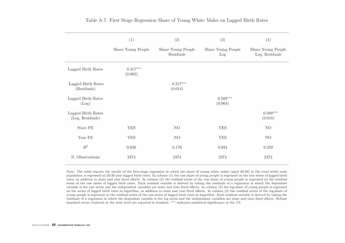
BANCO DE ESPAÑA 65 DOCUMENTO DE TRABAJO N.º 1837
Table A.7: First Stage Regression Share of Young White Males on Lagged Birth Rates
(1) (2) (3) (4)
Share Young People Share Young People Share Young People Share Young PeopleResiduals Log Log, Residuals
Lagged Birth Rates 0.317∗∗∗
(0.062)
Lagged Birth Rates 0.317∗∗∗
(Residuals) (0.014)
Lagged Birth Rates 0.509∗∗∗
(Log) (0.064)
Lagged Birth Rates 0.509∗∗∗
(Log, Residuals) (0.018)
State FE YES NO YES NO
Year FE YES NO YES NO
R2 0.938 0.176 0.934 0.259
N. Observations 2374 2374 2374 2374
Note: The table reports the results of the first-stage regression in which the share of young white males (aged 20-29) in the total white malepopulation is regressed on 20-30 year lagged birth rates. In column (1) the raw share of young people is regressed on the raw series of lagged birthrates, in addition to state and year fixed effects. In column (2) the residual series of the raw share of young people is regressed on the residualseries of the raw series of lagged birth rates. Each residual variable is derived by taking the residuals of a regression in which the dependentvariable is the raw series and the independent variables are state and time fixed effects. In column (3) the log-share of young people is regressedon the series of lagged birth rates in logarithm, in addition to state and year fixed effects. In column (4) the residual series of the log-share ofyoung people is regressed on the residual series of the raw series of lagged birth rates in logarithm. Each residual variable is derived by taking theresiduals of a regression in which the dependent variable is the log series and the independent variables are state and time fixed effects. Robuststandard errors clustered at the state level are reported in brackets. ∗∗∗ indicates statistical significance at the 1%.

BANCO DE ESPAÑA 66 DOCUMENTO DE TRABAJO N.º 1837
Table A.8: First Stage Regression Share of Young Males on Lagged Birth Rates
(1) (2) (3) (4)
Share Young People Share Young People Share Young People Share Young PeopleResiduals Log Log, Residuals
Lagged Birth Rates 0.280∗∗∗
(0.062)
Lagged Birth Rates 0.280∗∗∗
(Residuals) (0.013)
Lagged Birth Rates 0.446∗∗∗
(Log) (0.059)
Lagged Birth Rates 0.446∗∗∗
(Log, Residuals) (0.017)
State FE YES NO YES NO
Year FE YES NO YES NO
R2 0.913 0.159 0.915 0.228
N. Observations 2374 2374 2374 2374
Note: The table reports the results of the first-stage regression in which the share of young males (aged 20-29) in the total male population isregressed on 20-30 year lagged birth rates. In column (1) the raw share of young people is regressed on the raw series of lagged birth rates, inaddition to state and year fixed effects. In column (2) the residual series of the raw share of young people is regressed on the residual series of theraw series of lagged birth rates. Each residual variable is derived by taking the residuals of a regression in which the dependent variable is theraw series and the independent variables are state and time fixed effects. In column (3) the log-share of young people is regressed on the seriesof lagged birth rates in logarithm, in addition to state and year fixed effects. In column (4) the residual series of the log-share of young people isregressed on the residual series of the raw series of lagged birth rates in logarithm. Each residual variable is derived by taking the residuals of aregression in which the dependent variable is the log series and the independent variables are state and time fixed effects. Robust standard errorsclustered at the state level are reported in brackets. ∗∗∗ indicates statistical significance at the 1%.
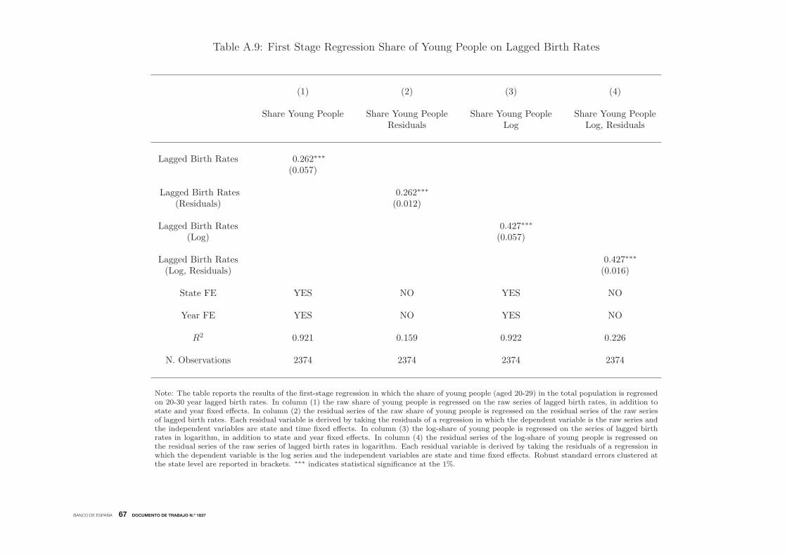
BANCO DE ESPAÑA 67 DOCUMENTO DE TRABAJO N.º 1837
Table A.9: First Stage Regression Share of Young People on Lagged Birth Rates
(1) (2) (3) (4)
Share Young People Share Young People Share Young People Share Young PeopleResiduals Log Log, Residuals
Lagged Birth Rates 0.262∗∗∗
(0.057)
Lagged Birth Rates 0.262∗∗∗
(Residuals) (0.012)
Lagged Birth Rates 0.427∗∗∗
(Log) (0.057)
Lagged Birth Rates 0.427∗∗∗
(Log, Residuals) (0.016)
State FE YES NO YES NO
Year FE YES NO YES NO
R2 0.921 0.159 0.922 0.226
N. Observations 2374 2374 2374 2374
Note: The table reports the results of the first-stage regression in which the share of young people (aged 20-29) in the total population is regressedon 20-30 year lagged birth rates. In column (1) the raw share of young people is regressed on the raw series of lagged birth rates, in addition tostate and year fixed effects. In column (2) the residual series of the raw share of young people is regressed on the residual series of the raw seriesof lagged birth rates. Each residual variable is derived by taking the residuals of a regression in which the dependent variable is the raw series andthe independent variables are state and time fixed effects. In column (3) the log-share of young people is regressed on the series of lagged birthrates in logarithm, in addition to state and year fixed effects. In column (4) the residual series of the log-share of young people is regressed onthe residual series of the raw series of lagged birth rates in logarithm. Each residual variable is derived by taking the residuals of a regression inwhich the dependent variable is the log series and the independent variables are state and time fixed effects. Robust standard errors clustered atthe state level are reported in brackets. ∗∗∗ indicates statistical significance at the 1%.

BANCO DE ESPAÑA 68 DOCUMENTO DE TRABAJO N.º 1837
B National Fiscal Multipliers
The fact that at the state level demographics have an effect on fiscal multipliers
which is statistically and economically significant does not necessarily imply that the
same applies also at the national level. In this Section we provide some suggestive
evidence showing that also national fiscal multipliers depend on demographics. To
do so, we run a SVAR a la Blanchard and Perotti (2002) on both a panel of developed
countries and a panel of developing countries. In either case, we show that the long-
run national output fiscal multiplier is larger in countries with higher shares of young
people in total population.
B.1 Data
We take the data from Ilzetzki et al. (2013). These authors compiled an unbalanced
panel on government spending, GDP, current account, real effective exchange rate,
and interest rates at quarterly frequency from 1960Q1 until 2009Q4 for 19 developed
countries and 25 developing countries.32 Then, we take the data on the demographic
structure of each country from the World Population Prospects prepared by the
32The developed countries are Australia, Belgium, Canada, Denmark, Finland, France, Germany, Greece,Iceland, Ireland, Israel, Italy, the Netherlands, Norway, Portugal, Spain, Sweden, the United Kingdom and theUnited States. The developing countries are Argentina, Botswana, Brazil, Bulgaria, Chile, Colombia, Croatia,Czech Republic, Ecuador, El Salvador, Estonia, Hungary, Latvia, Lithuania, Malaysia, Mexico, Peru, Poland,Romania, Slovakia, Slovenia, South Africa, Thailand, Turkey, and Uruguay.
Population Division of the Department of Economic and Social Affairs of the United
Nations Secretariat. The data on demographics are at the annual frequency from
1950 on.
B.2 Econometric Specification
We estimate fiscal multiplier using a SVAR system as in Blanchard and Perotti
(2002), such that
AXi,t =K∑k=1
CkXi,t−k +BUi,t

BANCO DE ESPAÑA 69 DOCUMENTO DE TRABAJO N.º 1837
where Xi,t is a vector that consists of the logarithm of real government expenditure,
the logarithm of real GDP, the ratio of the real current account balance over GDP,
and the log difference of the real effective exchange rate of country i. To identify
government spending shocks, we follow the identification assumption of Blanchard
and Perotti (2002): we assume that government spending reacts to changes in the
other macroeconomic variables with the delay of a quarter. This assumption defines
a Cholesky decomposition in which government spending is ordered first. For the
selection of the lag structure of the panel SVAR we follow Ilzetzki et al. (2013)
by choosing K = 4 lags. The results do not change if we choose a number of lags
between 1 and 8.
To identify the role of demographics on fiscal multipliers, we do the following.
First, we take all the developed countries and split them in two sets: 9 countries
with high shares of young people in total population, and 10 countries with low
share of young people in total population. Second, we estimate the SVAR system
on the two different panels and compare the results. Then, we repeat the same
exercise for the developing countries. In this case, we find 11 countries with high
shares of young people and 14 countries with low shares.33,34
Finally, we follow Ilzetzki et al. (2013) and define the long-run output fiscal
multiplier as∑∞
t=0 (1+ri)−tΔYi,t∑∞
t=0 (1+ri)−tΔGi,t
, where t = 0 denotes the date in which the government
expenditure shock occurs, and ri is the median of the country specific nominal
interest rate.
33We consider developed and developing countries separately because Ilzetzki et al. (2013) show that nationalfiscal multipliers in developed countries are large and positive, while in developing countries are large andnegative. The results of Ilzetzki et al. (2013) suggest that other factors (e.g., the exchange rate policy rule, thedegree of trade openness, and the level of public debt) could be explaining the differences in fiscal multipliersacross our sets of countries.
34Table B.10 reports countries’ average share of young people (age 20-29) over total population computedfrom 1970 to 2010. We show how we group the countries in the set with high shares of young people and theset with low shares of young people. In the case of developed countries, the nine countries with high sharesof young people have shares in the range of 15%-15.6%. Instead, the ten countries with low shares of youngpeople have shares in the range of 13.5%-14.7%. In the case of developing countries, the eleven countries withhigh shares of young people have shares in the range of 16.4%-17.2%. Instead, the fourteen countries with lowshares of young people have shares in the range of 14.7%-15.9%.

BANCO DE ESPAÑA 70 DOCUMENTO DE TRABAJO N.º 1837
B.2.1 Results
Figure B.1 reports the response of national output to an increase in government
spending in both developed countries and developing countries. We also report the
estimates of the long-run fiscal multiplier. Panel (a) shows the response in developed
countries with high shares of young people in total population whereas Panel (b)
plots the response in developed countries with low shares of young people in total
population.
Although the impact response is similar across groups, in countries with low
shares of young people the fiscal multipliers becomes statistically insignificant from
zero from the first quarter on, leading to a long-run multiplier of −0.11. Instead, incountries with high shares of young people the fiscal multiplier is always statistically
significant and the long-run multiplier equals 1.
Panel (c) and Panel (d) report the same set of results for developing countries.
As already pointed out in Ilzetzki et al. (2013), fiscal multipliers in developing
countries tend to be negative. Nevertheless, we find again that fiscal multipliers
vary with the demographic structure of the countries. In the developing countries
with high shares of young workers the impact responses are positive for the first
ten periods, and interestingly the point estimate of the cumulative fiscal multiplier
after two quarters is around 0.5, and is statistically different from zero. Then, the
responses turn into negative values and as a result the long-run multiplier is -0.39.
Instead, in the panel of developing countries with low shares of young people fiscal
multipliers are much smaller. The impact responses are always negative and in the
long-run the multiplier drops down to -1.2

BANCO DE ESPAÑA 71 DOCUMENTO DE TRABAJO N.º 1837
Figure B.1: National Fiscal Multipliers and Demographics.
(a) High Income Countries - High Share of Young (b) High Income Countries - Low Share of Young
(c) Low Income Countries - High Share of Young (d) Low Income Countries - Low Share of Young
Note: Panel (a) plots the cumulative national fiscal multipliers over twenty quarters following a government expen-diture shock in a panel of nine high income countries with high shares of young people (i.e., age 20-29) in totalpopulation. Panel (b) plots the cumulative national fiscal multipliers in a panel of eleven high income countries withlow shares of young people in total population. Panel (c) plots the cumulative national fiscal multipliers in a panelof eleven low income countries with high shares of young people in total population. Panel (d) plots the cumulativenational fiscal multipliers in a panel of fourteen low income countries with low shares of young people in total pop-ulation. In each Panel, the dotted lines display 90% confidence bands. The data on government expenditures andreal GDP at quarterly frequency from 1960 until 2009 across 19 high income countries and 25 low income countriesis from Ilzetzki et al. (2013).
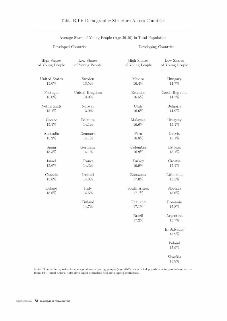
BANCO DE ESPAÑA 72 DOCUMENTO DE TRABAJO N.º 1837
Table B.10: Demographic Structure Across Countries
Average Share of Young People (Age 20-29) in Total Population
Developed Countries Developing Countries
High Shares Low Shares High Shares Low Sharesof Young People of Young People of Young People of Young People
United States Sweden Mexico Hungary15.0% 13.5% 16.4% 14.7%
Portugal United Kingdom Ecuador Czech Republic15.0% 13.9% 16.5% 14.7%
Netherlands Norway Chile Bulgaria15.1% 13.9% 16.6% 14.9%
Greece Belgium Malaysia Uruguay15.1% 14.1% 16.6% 15.1%
Australia Denmark Peru Latvia15.2% 14.1% 16.8% 15.1%
Spain Germany Colombia Estonia15.5% 14.1% 16.9% 15.1%
Israel France Turkey Croatia15.6% 14.3% 16.9% 15.1%
Canada Ireland Botswana Lithuania15.6% 14.3% 17.0% 15.5%
Iceland Italy South Africa Slovenia15.6% 14.5% 17.1% 15.6%
Finland Thailand Romania14.7% 17.1% 15.8%
Brazil Argentina17.2% 15.7%
El Salvador15.9%
Poland15.9%
Slovakia15.9%
Note: The table reports the average share of young people (age 20-29) over total population in percentage termsfrom 1970 until across both developed countries and developing countries.

BANCO DE ESPAÑA 73 DOCUMENTO DE TRABAJO N.º 1837
C More on the Household Sector
In this Section we provide the maximization problems and the optimal conditions
for each age group separately. We show that the optimal decisions of each individual
are linear in wealth, so we can linearly aggregate the optimal choices of individuals
within each age group to form a representative agent for each of the three age
groups. For the sake of exposition, we derive the aggregation results only for the
home economy. Nevertheless, the aggregation of the optimal choices of households
within each age group in the foreign economy follows the same procedure. We derive
all the problems and first-order conditions in real terms. We denote bjz,t =bjz,tPt
as
the real bond-holdings of an individual i in the age group z at time t, ajz,t =ajz,tPt
is the real total return on assets of an individual i in the age group z at time t,
rk,t =Rk,t
Ptis the real return on capital, and wt =
Wt
Ptis the real wage. Finally, as in
our calibration, we set ψc = ψI such that Pt = PI,t.
C.1 Old Agents
Assuming interior solutions for capital and bond holdings, the decision problem of
an old agent i is
maxcio,t,l
io,t,k
io,t+1,b
io,t+1
vio,t =
⎧⎨⎩(cio,t − χo
lio,t1+ 1
ν
1 + 1ν
)η
+ βωoEt[vio,t+1]
η
⎫⎬⎭1/η
(C.1)
subject to
cio,t + kio,t+1 + bo,t+1 +
ϕ
2
(kio,t+1
kio,t
− ϑo
)2kio,t
ωo
= aio,t + wtξolio,t − τ io,t
aio,t =
{kio,t [(1− δ) + rk,t] + bio,t
Rn,t
1 + πt
}(1
ωo
).
In order to solve the stochastic version of the problem we follow Farmer (1990)
closely. Define
fo(Qo,t) ≡(1 + (βωo)
11−ηQ
η1−η
o,t
) 1−ηη
(C.2)

BANCO DE ESPAÑA 74 DOCUMENTO DE TRABAJO N.º 1837
go(Qo,t) ≡(1 + (βωo)
11−ηQ
η1−η
o,t
)−1(C.3)
Qo,t ≡ Et
(fo(Qo,t+1)Rn,t+1
ωo(1 + πt+1)
)(C.4)
We conjecture that the old consume a fraction of a measure of wealth (Wo,t),
define as the sum of financial assets (aio,t) and the present value of human capital
gains (HC io,t), net of the present value of taxes (T i
o,t) and the present value of
adjustment costs (ADJ io,t). Moreover, the value function is given by
cio,t = εtςt[aio,t +HC i
o,t − T io,t − ADJ i
o,t
]= εtςtWo,t (C.5)
vio,t = (εtςt)−1η
(cio,t − χo
(lio,t)1+ 1
ν
1 + 1ν
)(C.6)
Finally we set (εtςt)η−1η ≡ fo(Qo,t), and thus go(Qo,t) = εtςt
Using the conjecture for the value and policy functions
vio,t = (εtςt)η−1η Wo,t − (εtςt)
−1η χo
(lio,t)1+ 1
ν
1 + 1ν
vio,t = fo(Qo,t)[aio,t +HC i
o,t − T io,t − ADJ i
o,t
]− (εtςt)−1η χo
(lio,t)1+ 1
ν
1 + 1ν
Rearranging the budget constraint we have that
aio,t+1 =Rn,t+1
(1 + πt+1)ωo
(aio,t + wtξol
io,t − τ io,t − adjio,t − cio,t
).
where adjio,t =(1− (1−δ+rk,t+1)(1+πt+1)
Rn,t+1
)kio,t+1 +
ϕ2
(kio,t+1
kio,t− ϑo
)2 kio,tωo
. Thus,
vio,t = fo(Qo,t)[ Rn,t
(1 + πt)ωo
(aio,t−1 + wt−1ξolio,t−1 − τ io,t−1 − adjio,t−1 − cio,t−1
)+
+HC io,t − T i
o,t − ADJ io,t
]− (εtςt)
−1η χo
(lio,t)1+ 1
ν
1 + 1ν
vio,t =fo(Qo,t)Rn,t
(1 + πt)ωo
(aio,t−1 + wt−1ξolio,t−1 − τ io,t−1 − adjio,t−1 − cio,t−1
)+
+fo(Qo,t)HC io,t − fo(Qo,t)T
io,t − fo(Qo,t)ADJ i
o,t − (εtςt)−1η χo
(lio,t)1+ 1
ν
1 + 1ν

BANCO DE ESPAÑA 75 DOCUMENTO DE TRABAJO N.º 1837
Taking expectations Et−1, and using (C.4)35
Et−1(vio,t) = Qo,t−1(aio,t−1 + wt−1ξolio,t−1 − τ io,t−1 − Et−1adjio,t−1 − cio,t−1
)+
+Et−1fo(Qo,t)HC io,t − Et−1fo(Qo,t)T
io,t − Et−1fo(Qo,t)ADJ i
o,t −
−Et−1
[(εtςt)
−1η χo
(lio,t)1+ 1
ν
1 + 1ν
]
Then, define
HC io,t ≡ wtξol
io,t + Et
[f(Qo,t+1)HC i
o,t+1
Qo,t
]+
+(Qo,tβωo)
11−η
Qo,t
[χo
(lio,t)1+ 1
ν
1 + 1ν
]− Et
[(εt+1ςt+1)
−1η χo
(lio,t+1)1+ 1
ν
1 + 1ν
]
T io,t ≡ τ io,t + Et
[f(Qo,t+1)T
io,t+1
Qo,t
]ADJ i
o,t ≡ Etadjio,t + Et
[f(Qo,t+1)ADJ i
o,t+1
Qo,t
]
Using these results and adding and subtracting (Qo,t−1βωo)1
1−η
[χo
(lio,t−1)1+ 1
ν
1+ 1ν
],
35We assume Et−1fo(Qo,t)Rn,t
(1+πt)ωoadjio,t−1 ≈ Qo,t−1Et−1adj
io,t−1, essentially ignoring the effect of uncertainty on
the portfolio allocation between bonds and capital. To a first order approximation the agent is indifferentbetween holding bonds or capital.
the expected value function simplifies to
Et−1(vio,t) =Qo,t−1(aio,t−1 +HC i
o,t−1 − T io,t−1 − ADJ i
o,t−1 − cio,t−1 −(Qo,t−1βωo)
11−η
Qo,t−1
[χo
(lio,t−1)1+ 1
ν
1 + 1ν
])=Qo,t−1
(Wo,t−1 − cio,t−1 −
(Qo,t−1βωo)1
1−η
Qo,t−1
[χo
(lio,t−1)1+ 1
ν
1 + 1ν
])
We can now use this result into the objective function to obtain
max vio,t =
⎧⎨⎩(cio,t − χo
lio,t1+ 1
ν
1 + 1ν
)η
+ βωo
[Qo,t
(Wo,t − cio,t −
(Qo,tβωo)1
1−η
Qo,t
χo
(lio,t)1+ 1
ν
1 + 1ν
)]η⎫⎬⎭1/η

BANCO DE ESPAÑA 76 DOCUMENTO DE TRABAJO N.º 1837
The first order condition with respect to consumption gives,
vio,t1−η⎛⎝(cio,t − χo
lio,t1+ 1
ν
1 + 1ν
)η−1
+ βωo
[Qo,t
(Wo,t − cio,t −
(Qo,tβωo)1
1−η
Qo,t
χo
(lio,t)1+ 1
ν
1 + 1ν
)]η−1(−Qo,t)
⎞⎠ = 0
(cio,t − χo
lio,t1+ 1
ν
1 + 1ν
)= (βωoQo,t)
1η−1
[Qo,t
(Wo,t − cio,t −
(Qo,tβωo)1
1−η
Qo,t
χo
(lio,t)1+ 1
ν
1 + 1ν
)]
cio,t =(1 + (βωo)
11−ηQ
η1−η
o,t
)−1Wo,t = εtςtWo,t
We can now replace the solution for cio,t, which matches our conjecture, into the
value function to obtain
vio,t =
⎡⎣(cio,t − χo
lio,t1+ 1
ν
1 + 1ν
)η
+ βωo
[Qo,t
([1 + (βωo)
11−ηQ
η1−η
o,t ]cio,t − cio,t −(Qo,tβωo)
11−η
Qo,t
χo
(lio,t)1+ 1
ν
1 + 1ν
)]η⎤⎦1/η
vio,t =
⎧⎨⎩(1 + (βωo)1
1−ηQη
1−η
o,t
)(cio,t − χo
lio,t1+ 1
ν
1 + 1ν
)η⎫⎬⎭
1/η
Using the definition for fo(Qo,t) we confirm our guess, obtaining
vio,t = (εtςt)−1η
(cio,t − χo
(lio,t)1+ 1
ν
1 + 1ν
)
Combining (C.2) and (C.4) we obtain the condition that determines the marginal
propensity to consume of the old.
Qo,t = ((εtςt)−1 − 1)
1−ηη (βωo)
−1η
((εtςt)−1 − 1)
1−ηη = Et
(Rn,t+1(βωo)
1η (εtςt)
η−1η
ωo(1 + πt+1)
)
Finally, from the first order conditions of (C.1) labor is set such that
lio,t =
(ξowt
χo
)ν
,
and, to a first order approximation the individual is indifferent between holding
bonds or capital. The no-arbitrage condition on investment posits that the expected
return on capital should equalize the expected return on bonds, that is,

BANCO DE ESPAÑA 77 DOCUMENTO DE TRABAJO N.º 1837
(Rn,t+1
1 + πt+1
)=
⎛⎜⎝(1− δ) + rk,t+1 − ϕ2
(kio,t+2
kio,t+1− ϑo
)2+ ϕ
(kio,t+2
kio,t+1− ϑo
)kio,t+2
kio,t+1[1 + ϕ
ωo
(kio,t+1
kio,t− ϑo
)]⎞⎟⎠
If the constraint binds, we no longer have an interior solution. In this case the
consumption policy function can be easily obtained from the budget constraint of
the agent. The labor optimality condition remains the same.
C.2 Mature Agents
The decision problem of a mature agent i, assuming interior solutions for capital
and bond holdings, is
maxcim,t,l
im,t,k
im,t+1,b
im,t+1
vim,t =
{(cim,t − χm
lim,t1+ 1
ν
1 + 1ν
)η
+ βEt[ωmvim,t+1 + (1− ωm)v
io,t+1]
η
}1/η
(C.7)
subject to
kim,t+1 + bim,t+1 + cim,t +
ϕ
2
(kim,t+1
kim,t
− ϑm
)2
kim,t = aiw,t + wtl
im,t + (1− τd)d
im,t − τ im,t
aim,t = kim,t((1− δ) + rk,t) + bim,t
Rnt
1 + πt
.
Define
fm(Qm,t) ≡(1 + (β)
11−ηQ
η1−η
m,t
) 1−ηη
(C.8)
gm(Qm,t) ≡(1 + (β)
11−ηQ
η1−η
m,t
)−1(C.9)
Qm,t ≡ Et
(Zt+1Rn,t+1fm(Qm,t+1)
(1 + πt+1)
)(C.10)
where Zt+1 = (ωm + (1− ωm)εη−1η
t+1 ).
We conjecture that the mature consume a fraction of a measure of wealth (Wm,t),
define as the sum of financial assets (aim,t), the present value of human capital gains
(HC im,t) and dividends (Di
m,t), net of the present value of taxes (T im,t) and the
present value of adjustment costs (ADJ im,t). Moreover, the value function is given

BANCO DE ESPAÑA 78 DOCUMENTO DE TRABAJO N.º 1837
cim,t = ςt[aim,t +HC i
m,t +Dim,t − T i
m,t − ADJ im,t
]= ςtWm,t (C.11)
vim,t = (ςt)−1η
(cim,t − χo
(lim,t)1+ 1
ν
1 + 1ν
)(C.12)
Finally we set (ςt)η−1η ≡ fm(Qm,t), and thus gm(Qm,t) = ςt.
Using the conjecture for the value and policy functions
vim,t = (ςt)η−1η Wm,t − (ςt)
−1η χm
(lim,t)1+ 1
ν
1 + 1ν
vim,t = fm(Qm,t)[aim,t +HC i
m,t +Dim,t − T i
m,t − ADJ im,t
]− (ςt)−1η χm
(lim,t)1+ 1
ν
1 + 1ν
by
Rearranging the budget constraint, we have that
aim,t+1 =Rn,t+1
(1 + πt+1)
(aim,t + wtl
im,t + (1− τd)d
im,t − τ im,t − adjim,t − cim,t
).
where adjim,t =(1− (1−δ+rk,t+1)(1+πt+1)
Rn,t+1
)kim,t+1 +
ϕ2
(kim,t+1
kim,t− ϑm
)2kim,t.
Thus,
vim,t = fm(Qm,t)[ Rn,t
(1 + πt)
(aim,t−1 + wt−1lim,t−1 + (1− τd)d
im,t − τ im,t−1 − adjim,t−1 − cim,t−1
)+
+HC im,t +Di
m,t − T im,t − ADJ i
m,t
]− (ςt)
−1η χm
(lim,t)1+ 1
ν
1 + 1ν
vim,t =fm(Qm,t)Rn,t
(1 + πt)
(aim,t−1 + wt−1lim,t−1 + (1− τd)d
im,t − τ im,t−1 − adjim,t−1 − cim,t−1
)+
+fm(Qm,t)(HC i
m,t +Dm,t − T im,t − ADJ i
m,t
)− (ςt)−1η χm
(lim,t)1+ 1
ν
1 + 1ν
The value function of the old at time t who was a mature individual at time t−1
can be written as 36
1
36We assume that adjim,t−1 ≈ adjim,t−1|o,t for an individual transitioning from mature to the old age. Thedifference might only arise due to the second order effects when the covariance between the rates of return onbonds and capital is considered.

BANCO DE ESPAÑA 79 DOCUMENTO DE TRABAJO N.º 1837
vio,t |m,t−1 = fo(Qo,t)[aio,t +HC i
o,t − T io,t − ADJ i
o,t
]− (εtςt)−1η χo
(lio,t)1+ 1
ν
1 + 1ν
vio,t |m,t−1 =fo(Qo,t)Rn,t
(1 + πt)
(aim,t−1 + wt−1lim,t−1 + (1− τd)d
im,t − τ im,t−1 − adjim,t−1 − cim,t−1
)+
+fo(Qo,t)HC io,t − fo(Qo,t)T
io,t − fo(Qo,t)ADJ i
o,t − (εtςt)−1η χo
(lio,t)1+ 1
ν
1 + 1ν
We can now obtain [ωmvim,t + (1− ωm)v
io,t],
ωmvim,t + (1− ωm)v
io,t =
=(ωmfm(Qm,t) + (1− ωm)fo(Qo,t))Rn,t
(1 + πt)
(aim,t−1 + wt−1lim,t−1+
+ (1− τd)dim,t − τ im,t−1 − adjim,t−1 − cim,t−1
)− ωm(ςt)
−1η χm
(lim,t)1+ 1
ν
1 + 1ν
+
+ ωm
(fm(Qm,t)HC i
m,t + fm(Qm,t)Dm,t − fm(Qm,t)Tim,t − fm(Qm,t)ADJ i
m,t
)+
+ (1− ωm)(fo(Qo,t)HC i
o,t − fo(Qo,t)Tio,t − fo(Qo,t)ADJ i
o,t
)− (1− ωm)(εtςt)−1η χo
(lio,t)1+ 1
ν
1 + 1ν
Note that
(ωmfm(Qm,t) + (1− ωm)fo(Qo,t))Rn,t
(1 + πt)=
(ωm(ςt)η−1η + (1− ωm)(εtςt)
η−1η )Rn,t
(1 + πt)
=Zt(ςt)
η−1η Rn,t
(1 + πt)=
Ztfm(Qm,t)Rn,t
(1 + πt)
Therefore, taking expectations Et−1, and using (C.10)37
Et−1[ωmvim,t + (1− ωm)v
io,t] =
= Qm,t−1(aim,t−1 + wt−1lim,t−1 + (1− τd)d
im,t − τ im,t−1 − Et−1adjim,t−1 − cim,t−1
)+
+ Et−1ωmfm(Qm,t)(HC i
m,t +Dm,t − T im,t − ADJ i
m,t
)− Et−1ωm(ςt)−1η χm
(lim,t)1+ 1
ν
1 + 1ν
+ Et−1(1− ωm)fo(Qo,t)(HC i
o,t − T io,t − ADJ i
o,t
)− Et−1(1− ωm)(εtςt)−1η χo
(lio,t)1+ 1
ν
1 + 1ν
37Once again, we assume Et−1fm(Qm,t)Rn,t
(1+πt)adjim,t−1 ≈ Qm,t−1Et−1adj
im,t−1, essentially ignoring the effect of
uncertainty on the portfolio allocation between bonds and capital. To a first order approximation the agent isindifferent between holding bonds or capital.

BANCO DE ESPAÑA 80 DOCUMENTO DE TRABAJO N.º 1837
Then, define
HC im,t ≡ wtl
im,t + EtωM
f(Qm,t+1)HC im,t+1
Qm,t
+ Et(1− ωM)f(Qo,t+1)HC i
o,t+1
Qm,t
−
−Et(ςt)
−1η
Qm,t
[ωMχm
(lim,t+1)1+ 1
ν
1 + 1ν
+ (εt+1)−1η (1− ωM)χo
(lio,t+1)1+ 1
ν
1 + 1ν
]+
+(Qm,tβ)
11−η
Qm,t
[χm
(lim,t)1+ 1
ν
1 + 1ν
]
Dim,t ≡ (1− τd)d
im,t + Et
ωMf(Qm,t+1)Dim,t+1
Qm,t
T im,t ≡ τ im,t + Et
ωMf(Qm,t+1)Tim,t+1
Qm,t
+ Et
(1− ωM)f(Qo,t+1)Tio,t+1
Qm,t
ADJ im,t ≡ Etadj
im,t + Et
ωMf(Qm,t+1)ADJ im,t+1
Qm,t
+ Et
(1− ωM)f(Qo,t+1)ADJ io,t+1
Qm,t
Using these results and adding and subtracting (Qm,t−1β)1
1−η
[χm
(lim,t−1)1+ 1
ν
1+ 1ν
], we
obtain
Et−1[ωmvim,t + (1− ωm)v
io,t] =
= Qm,t−1(aim,t−1 +HC i
m,t−1 +Dim,t−1 − T i
m,t−1−
− ADJ im,t−1 − cim,t−1 −
(Qm,t−1β)1
1−η
Qm,t−1
[χm
(lim,t−1)1+ 1
ν
1 + 1ν
])= Qm,t−1
(Wm,t−1 − cim,t−1 −
(Qm,t−1β)1
1−η
Qm,t−1
[χm
(lim,t−1)1+ 1
ν
1 + 1ν
])
We can now use this result into the Bellman equation to obtain
max vim,t =
⎧⎨⎩(cim,t − χm
lim,t1+ 1
ν
1 + 1ν
)η
+ β
[Qm,t
(Wm,t − cim,t −
(Qm,tβ)1
1−η
Qm,t
χm
(lim,t)1+ 1
ν
1 + 1ν
)]η⎫⎬⎭1/η
The first order condition with respect to consumption allow us to obtain,
cim,t =(1 + (β)
11−ηQ
η1−η
m,t
)−1Wm,t = ςtWm,t

BANCO DE ESPAÑA 81 DOCUMENTO DE TRABAJO N.º 1837
We can now replace the solution for cim,t, which matches our conjecture, into the
value function to obtain
vim,t = (ςt)−1η
(cim,t − χm
(lim,t)1+ 1
ν
1 + 1ν
)
Combining (C.8) and (C.10) we obtain the condition that determines the marginal
propensity to consume of the mature agents.
Qm,t = ((ςt)−1 − 1)
1−ηη (β)
−1η
((ςt)−1 − 1)
1−ηη = Et
(Zt+1Rn,t+1(β)
1η (ςt)
η−1η
(1 + πt+1)
)
Finally, from the first order conditions of (C.7) labor is set such that
lim,t =
(wt
χm
)ν
,
and, to a first order approximation the individual is indifferent between holding
bonds or capital. The no-arbitrage condition on investment posits that the expected
return on capital should equalize the expected return on bonds, that is,
(Rn,t+1
1 + πt+1
)=
⎛⎜⎝(1− δ) + rk,t+1 − ϕ2
(kim,t+2
kim,t+1− ϑm
)2+ ϕ
(kim,t+2
kim,t+1− ϑm
)kim,t+2
kim,t+1(1 + ϕ
(kim,t+1
kim,t− ϑm
))⎞⎟⎠
(C.13)
If the constraint binds, we no longer have an interior solution. In this case the
consumption policy function can be easily obtained from the budget constraint of
the agent. The labor optimality condition remains the same.
C.3 Young Agents
For the problem of the young we follow a similar procedure to obtain
fy(Qy,t) ≡ (εy,tςt)η−1η (C.14)
Qy,t = ((εy,tςt)−1 − 1)
1−ηη (β)
−1η (C.15)
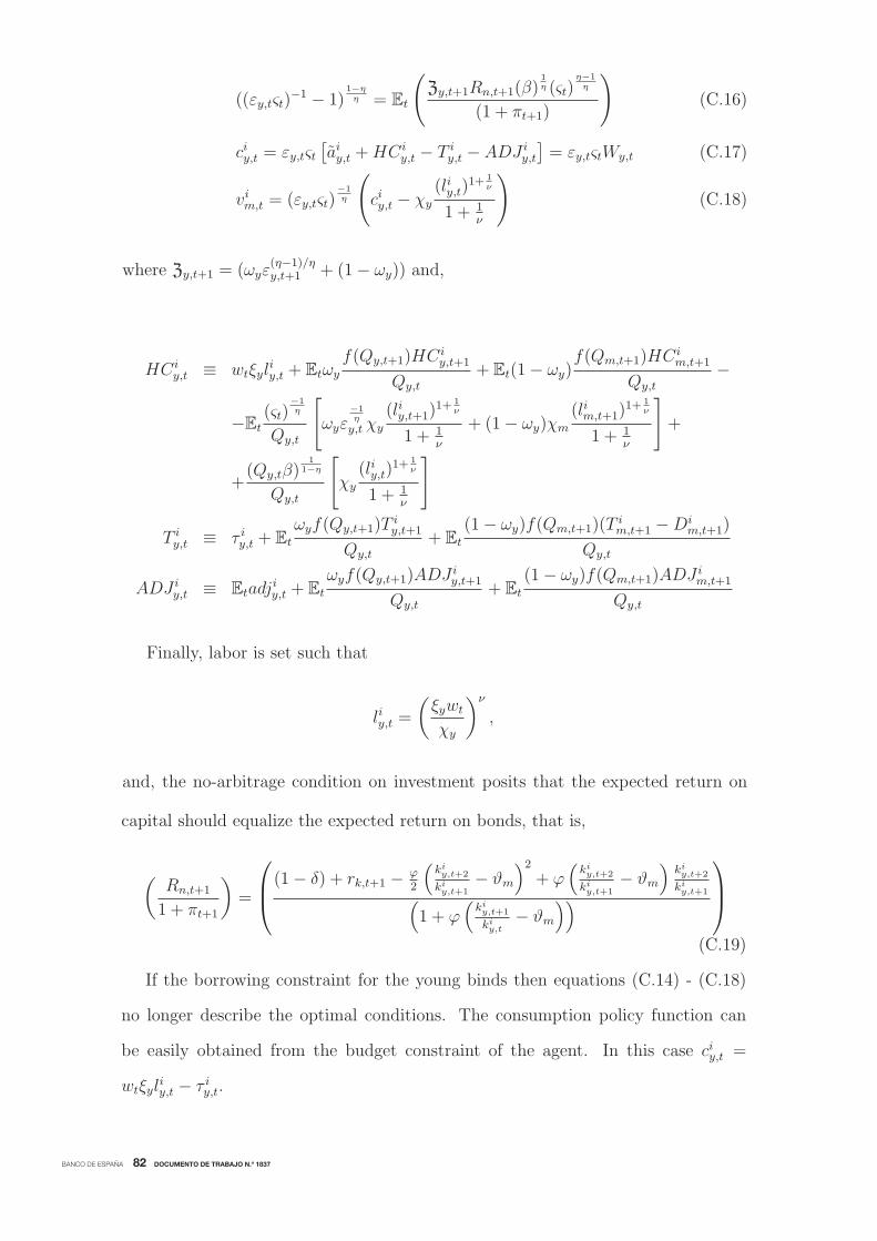
BANCO DE ESPAÑA 82 DOCUMENTO DE TRABAJO N.º 1837
((εy,tςt)−1 − 1)
1−ηη = Et
(Zy,t+1Rn,t+1(β)
1η (ςt)
η−1η
(1 + πt+1)
)(C.16)
ciy,t = εy,tςt[aiy,t +HC i
y,t − T iy,t − ADJ i
y,t
]= εy,tςtWy,t (C.17)
vim,t = (εy,tςt)−1η
(ciy,t − χy
(liy,t)1+ 1
ν
1 + 1ν
)(C.18)
where Zy,t+1 = (ωyε(η−1)/ηy,t+1 + (1− ωy)) and,
HC iy,t ≡ wtξyl
iy,t + Etωy
f(Qy,t+1)HC iy,t+1
Qy,t
+ Et(1− ωy)f(Qm,t+1)HC i
m,t+1
Qy,t
−
−Et(ςt)
−1η
Qy,t
[ωyε
−1η
y,t χy
(liy,t+1)1+ 1
ν
1 + 1ν
+ (1− ωy)χm
(lim,t+1)1+ 1
ν
1 + 1ν
]+
+(Qy,tβ)
11−η
Qy,t
[χy
(liy,t)1+ 1
ν
1 + 1ν
]
T iy,t ≡ τ iy,t + Et
ωyf(Qy,t+1)Tiy,t+1
Qy,t
+ Et
(1− ωy)f(Qm,t+1)(Tim,t+1 −Di
m,t+1)
Qy,t
ADJ iy,t ≡ Etadj
iy,t + Et
ωyf(Qy,t+1)ADJ iy,t+1
Qy,t
+ Et
(1− ωy)f(Qm,t+1)ADJ im,t+1
Qy,t
Finally, labor is set such that
liy,t =
(ξywt
χy
)ν
,
and, the no-arbitrage condition on investment posits that the expected return on
capital should equalize the expected return on bonds, that is,
(Rn,t+1
1 + πt+1
)=
⎛⎜⎝(1− δ) + rk,t+1 − ϕ2
(kiy,t+2
kiy,t+1− ϑm
)2+ ϕ
(kiy,t+2
kiy,t+1− ϑm
)kiy,t+2
kiy,t+1(1 + ϕ
(kiy,t+1
kiy,t− ϑm
))⎞⎟⎠
(C.19)
If the borrowing constraint for the young binds then equations (C.14) - (C.18)
no longer describe the optimal conditions. The consumption policy function can
be easily obtained from the budget constraint of the agent. In this case ciy,t =
wtξyliy,t − τ iy,t.

BANCO DE ESPAÑA 83 DOCUMENTO DE TRABAJO N.º 1837
C.4 Aggregation
In this Section we show that we can linearly aggregate the optimal choices of in-
dividuals across each age group, such that for a variable xz,t we have that xz,t =∫ Nz,t
0xiy,t di.
Firstly we must ensure that at steady state adjustment costs are zero. Given the
arbitrage conditions (C.1), (C.13), and its counterpart for the young problem, we
have that the ratio of capital for any agent within a type is constant, which is to
say thatkiy,t+1
kiy,t= ky,t+1
ky,t,
kim,t+1
kim,t= km,t+1
km,t, and
kio,t+1
kio,t= ko,t+1
ko,t, where ky,t+1
ky,t, km,t+1
km,t, and
ko,t+1
ko,tdefine given age-group specific values for the ratio of physical capital holdings
over time. Then given that individuals are born with no capital at steady state we
have that
ky,t+1 =
∫ Ny,t
0
kiy,t+1 =
∫ Ny,t+1
0
kiy,t+2 = ky,t+2 = ky,SS
As the young individuals who become mature are selected randomly
ky,SS =
∫ Ny,t+1
0
kiy,t+2 =
∫ ωyNy,t+1
0
ky,t+1
ky,tkiy,t+1 = ωy
ky,t+1
ky,t
∫ Ny,t
0
kiy,t+1 = ωy
ky,t+1
ky,tky,SS
Hence, ky,t+1
ky,t|SS= 1
ωy. For mature agents we have that
km,t+1 =
∫ Nm,t
0
kim,t+1 =
∫ Nm,t+1
0
kim,t+2 = km,t+2 = kmy,SS
where
km,SS =
∫ Nm,t+1
0
kim,t+2 =
∫ ωmNm,t+1
0
km,t+1
km,t
kim,t+1 +
∫ (1−ωy)Ny,t+1
0
ky,t+1
ky,tkiy,t+1 = . . .
. . . = ωmkm,t+1
km,t
∫ Nm,t
0
kim,t+1 + (1− ωy)
ky,t+1
ky,t
∫ Ny,t
0
kiy,t+1 = . . .
. . . = ωmkm,t+1
km,t
km,SS +(1− ωy)
ωy
ky,SS.
As a result, we have that
km,t+1
km,t
|SS= 1
ωm
(1− (1− ωy)
ωy
ky,SSkm,SS
).

BANCO DE ESPAÑA 84 DOCUMENTO DE TRABAJO N.º 1837
Analogously, we have that
ko,t+1
ko,t|SS= 1
ωo
(1− (1− ωm)
km,t+1
km,t
|SS km,SS
ko,SS
).
Thus, if we set
ϑy =1
ωy
ϑm =1
ωm
(1− (1− ωy)
ωy
ky,SSkm,SS
)ϑo =
1
ωo
(1− (1− ωm)ϑm
km,SS
ko,SS
)
we ensure that at steady state capital adjustment costs are zero. At steady state
agents accumulate or reduce capital at a constant rate while within a group z ∈{y,m, o}. Nonetheless, as individuals transition across groups through their life
cycle, the aggregate capital holdings of each group remain constant and no adjust
cost of capital is paid.
Ensuring that at steady state adjustment costs are zero is important for aggrega-
tion since the only non-linear term left in the consumption decision is the quadratic
term in the adjustment cost condition. As we solve a linearized version of the model
around the steady state this quadratic term disappears such that the choice vari-
ables across agents within a group can be easily aggregated to find a condition for
each group. Consequently, for instance, the aggregate consumption of all old agents
at time t is simply given by
co,t = εtςt [ao,t +HCo,t − To,t − ADJo,t] .
where we excluded the quadratic terms which are irrelevant in a first order ap-
proximated solution and thus, ADJo,t = ˜adjo,t +(1+πt+1)ωo
Rn,t+1ADJo,t+1 and ˜adj
i
o,t =(1− (1−δ+rk,t+1)(1+πt+1)
Rn,t+1
)kio,t+1. Therefore, the equilibrium conditions can be defined
without explicitly incorporating the heterogeneity within age groups.

BANCO DE ESPAÑA 85 DOCUMENTO DE TRABAJO N.º 1837
As some young agents become mature and some mature agents become old every
period, when we aggregate and discard the quadratic adjustment terms, the flow of
assets are given by
ky,t+1 + by,t+1 = ωy(ay,t + ly,tξywt + τy,t − cy,t) (C.20)
ay,t = ky,t [(1− δ) + rk,t] + by,tRn,t+1
1 + πt+1
(C.21)
km,t+1 + bm,t+1 = ωm(am,t + lm,twt + dm,t + τm,t − cm,t) + . . . (C.22)
· · ·+ (1− ωy)(ay,t + ly,tξywt + τy,t − cy,t) (C.23)
am,t = km,t [(1− δ) + rk,t] + bm,tRn,t+1
1 + πt+1
(C.24)
ko,t+1 + bo,t+1 = ao,t + ξolo,twt + tro,t − co,t + . . . (C.25)
· · ·+ (1− ωm)(am,t + lm,twt + dm,t + τm,t − cm,t) (C.26)
ao,t = ko,t [(1− δ) + rk,t] + bo,tRn,t+1
1 + πt+1
(C.27)
We then define the stochastic discount factor for the mature group as
Qmt = βZt+1
[ωm
(cm,t+1 − χm
lm,t+11+ 1
ν
1+ 1ν
)+ (1− ωm)ε
−1η
t+1
(co,t+1 − χo
lo,t+11+ 1
ν
1+ 1ν
)](1−η)(cm,t − χm
lm,t1+ 1
ν
1+ 1ν
)(1−η)
Finally, given that we are interested in a solution under a linear approximation,
(kim,t+1
kim,t
− ϑm
)=
(km,t+1
km,t
− ϑm
)≈ ϑm
(km,t+1 − km,t+1 |SS
km,t+1 |SS− km,t − km,t |SS
km,t |SS
)
= ϑm
(1
Nm,t
km,t+1 − km,t+1 |SSkm,t+1 |SS − 1
Nm,t−1
km,t − km,t |SSkm,t |SS
)≈ ϑm
(km,t+1Nm,t−1km,tNm,t
− 1
)
then the aggregated arbitrage condition for mature agents becomes
Rn,t+1
1 + πt+1
=(1− δ) + rk,t+1 + ϕϑ2
m
(km,t+1
km,t
Nm,t
Nm,t+1− 1)
km,t+1
km,t
Nm,t
Nm,t+1(1 + ϑmϕ
(km,t
km,t−1
Nm,t−1
Nm,t− 1)) (C.28)

BANCO DE ESPAÑA 86 DOCUMENTO DE TRABAJO N.º 1837
38Given the probabilistic nature of the death transition, a very small share of old individuals might live fora very long time. In such cases assets would eventually be completely consumed and the borrowing constraintwould bind. As the mass of old individuals in this situation is very small, for simplicity we assume the inter-mediary that offers the annuity provides consumption to the old individuals living for too long such that thecondition (C.5) always holds within this age group.
Given the hump-shaped life-cycle earnings profile, the young wants to borrow,
the mature wants to save for retirement and the old dissaves (see Constantinides
et al. (2002) for an simple OLG model with the same features). Thus, ay,t = 0
and from (C.20) we obtain the consumption of the young. (C.23) simplifies to
km,t+1 + bm,t+1 = ωm(am,t + lm,twt + dm,t + τm,t − cm,t).38

BANCO DE ESPAÑA 87 DOCUMENTO DE TRABAJO N.º 1837
D More on Calibration
This Section reports the values of the entire set of parameters of the model. Table
D.11 reports the calibration choices of the block of parameters that comes with the
structure of a standard open-economy New Keynesian model. Table D.12 reports
the calibration choices of the set of parameters that govern the demographic and
life-cycle structure of the model.

BANCO DE ESPAÑA 88 DOCUMENTO DE TRABAJO N.º 1837
Table D.11: Calibration - Standard Parameters
Parameter Value Target/Source
Time Discount Factor β = 0.995 Standard Value
Elasticity Intertemporal Substitution η = −9 EIS = 0.1
Capital Depreciation Rate δ = 0.025 Standard Value
Capital Adjustment Cost ϕ = 122 Two-Year NationalInvestment Fiscal Multiplier = -0.9
Home Bias in Consumption & Investment λ = 0.69 Nakamura and Steinsson (2014)
Elasticity Substitution ψc = 2 Nakamura and Steinsson (2014)Home & Foreign Consumption
Elasticity Substitution ψi = 2 ψi = ψc
Home & Foreign Investment
Elasticity Substitution ε = 9 Standard ValueAcross Varieties
Capital Share in Production α = 0.32 Standard Value
Calvo Parameter ζ = 0.75 Standard Value
Dividend Tax Rate τd = 0.9394 Mature Agents Receive60% Total Dividends
Steady-State GovernmentGH,SS+GF,SS
Y uSS
= 0.204 Data
Spending to Output Ratio
Persistence Government ρG = 0.953 DataSpending Shock
Inertia of Government Debt ρbg = 0.95 Dynamic Response to Spendingof Government Debt
Response to Spending φG = 4.5 Dynamic Response to Spendingof Government Debt of Government Debt
Response to Spending φT = 0.01 Dynamic Response to Spendingof Taxation of Taxation
Inertia of Taylor Rule ψR = 0.8 Clarida et al. (2000)
Taylor Rule Response ψπ = 1.5 Clarida et al. (2000)to Inflation
Taylor Rule Response ψY = 0.2 Clarida et al. (2000)to Output Gap
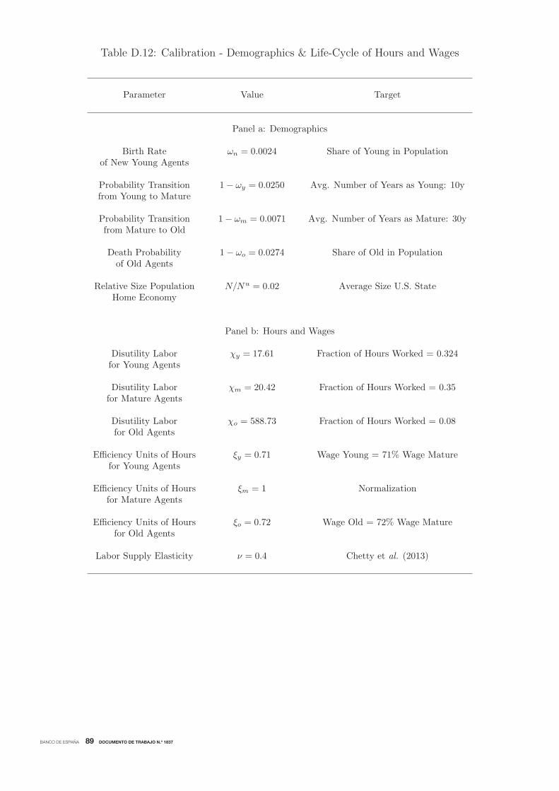
BANCO DE ESPAÑA 89 DOCUMENTO DE TRABAJO N.º 1837
Table D.12: Calibration - Demographics & Life-Cycle of Hours and Wages
Parameter Value Target
Panel a: Demographics
Birth Rate ωn = 0.0024 Share of Young in Populationof New Young Agents
Probability Transition 1− ωy = 0.0250 Avg. Number of Years as Young: 10yfrom Young to Mature
Probability Transition 1− ωm = 0.0071 Avg. Number of Years as Mature: 30yfrom Mature to Old
Death Probability 1− ωo = 0.0274 Share of Old in Populationof Old Agents
Relative Size Population N/Nu = 0.02 Average Size U.S. StateHome Economy
Panel b: Hours and Wages
Disutility Labor χy = 17.61 Fraction of Hours Worked = 0.324for Young Agents
Disutility Labor χm = 20.42 Fraction of Hours Worked = 0.35for Mature Agents
Disutility Labor χo = 588.73 Fraction of Hours Worked = 0.08for Old Agents
Efficiency Units of Hours ξy = 0.71 Wage Young = 71% Wage Maturefor Young Agents
Efficiency Units of Hours ξm = 1 Normalizationfor Mature Agents
Efficiency Units of Hours ξo = 0.72 Wage Old = 72% Wage Maturefor Old Agents
Labor Supply Elasticity ν = 0.4 Chetty et al. (2013)

BANCO DE ESPAÑA PUBLICATIONS
WORKING PAPERS
1801 OLYMPIA BOVER, LAURA HOSPIDO and ERNESTO VILLANUEVA: The impact of high school financial education on
financial knowledge and choices: evidence from a randomized trial in Spain.
1802 IGNACIO HERNANDO, IRENE PABLOS, DANIEL SANTABÁRBARA and JAVIER VALLÉS: Private Saving. New Cross-
Country Evidence Based on Bayesian Techniques.
1803 PABLO AGUILAR and JESÚS VÁZQUEZ: Term structure and real-time learning.
1804 MORITZ A. ROTH: International co-movements in recessions.
1805 ANGELA ABBATE and DOMINIK THALER: Monetary policy and the asset risk-taking channel.
1806 PABLO MARTÍN-ACEÑA: Money in Spain. New historical statistics. 1830-1998.
1807 GUILHERME BANDEIRA: Fiscal transfers in a monetary union with sovereign risk.
1808 MIGUEL GARCÍA-POSADA GÓMEZ: Credit constraints, fi rm investment and growth: evidence from survey data.
1809 LAURA ALFARO, MANUEL GARCÍA-SANTANA and ENRIQUE MORAL-BENITO: On the direct and indirect real
effects of credit supply shocks.
1810 ROBERTO RAMOS and CARLOS SANZ: Backing the incumbent in diffi cult times: the electoral impact of wildfi res.
1811 GABRIEL JIMÉNEZ, ENRIQUE MORAL-BENITO and RAQUEL VEGAS: Bank lending standards over the cycle:
the role of fi rms’ productivity and credit risk.
1812 JUAN S. MORA-SANGUINETTI and ROK SPRUK: Industry vs services: do enforcement institutions matter for
specialization patterns? Disaggregated evidence from Spain.
1813 JAMES CLOYNE, CLODOMIRO FERREIRA and PAOLO SURICO: Monetary policy when households have debt: new
evidence on the transmission mechanism.
1814 DMITRI KIRPICHEV and ENRIQUE MORAL-BENITO: The costs of trade protectionism: evidence from Spanish fi rms
and non-tariff measures.
1815 ISABEL ARGIMÓN, CLEMENS BONNER, RICARDO CORREA, PATTY DUIJM, JON FROST, JAKOB DE HAAN,
LEO DE HAAN and VIKTORS STEBUNOVS: Financial institutions’ business models and the global transmission of
monetary policy.
1816 JOSE ASTURIAS, MANUEL GARCÍA-SANTANA and ROBERTO RAMOS: Competition and the welfare gains from
transportation infrastructure: evidence from the Golden Quadrilateral of India.
1817 SANDRA GARCÍA-URIBE: Multidimensional media slant: complementarities in news reporting by US newspapers .
1818 PILAR CUADRADO, AITOR LACUESTA, MARÍA DE LOS LLANOS MATEA and F. JAVIER PALENCIA-GONZÁLEZ:
Price strategies of independent and branded dealers in retail gas market. The case of a contract reform in Spain.
1819 ALBERTO FUERTES, RICARDO GIMENO and JOSÉ MANUEL MARQUÉS: Extraction of infl ation expectations from
fi nancial instruments in Latin America.
1820 MARIO ALLOZA, PABLO BURRIEL and JAVIER J. PÉREZ: Fiscal policies in the euro area: revisiting the size of spillovers.
1821 MARTA MARTÍNEZ-MATUTE and ALBERTO URTASUN: Uncertainty, fi rm heterogeneity and labour adjustments.
Evidence from European countries.
1822 GABRIELE FIORENTINI, ALESSANDRO GALESI, GABRIEL PÉREZ-QUIRÓS and ENRIQUE SENTANA: The rise and fall
of the natural interest rate.
1823 ALBERTO MARTÍN, ENRIQUE MORAL-BENITO and TOM SCHMITZ: The fi nancial transmission of housing bubbles:
evidence from Spain.
1824 DOMINIK THALER: Sovereign default, domestic banks and exclusion from international capital markets.
1825 JORGE E. GALÁN and JAVIER MENCÍA: Empirical assessment of alternative structural methods for identifying cyclical
systemic risk in Europe.
1826 ROBERTO BLANCO and NOELIA JIMÉNEZ: Credit allocation along the business cycle: evidence from the latest boom
bust credit cycle in Spain.
1827 ISABEL ARGIMÓN: The relevance of currency-denomination for the cross-border effects of monetary policy.
1828 SANDRA GARCÍA-URIBE: The effects of tax changes on economic activity: a narrative approach to frequent anticipations.
1829 MATÍAS CABRERA, GERALD P. DWYER and MARÍA J. NIETO: The G-20 regulatory agenda and bank risk.
1830 JACOPO TIMINI and MARINA CONESA: Chinese exports and non-tariff measures: testing for heterogeneous effects at the
product level.
1831 JAVIER ANDRÉS, JOSÉ E. BOSCÁ, JAVIER FERRI and CRISTINA FUENTES-ALBERO: Households’ balance sheets and
the effect of fi scal policy.

1832 ÓSCAR ARCE, MIGUEL GARCÍA-POSADA, SERGIO MAYORDOMO and STEVEN ONGENA: Adapting lending policies
when negative interest rates hit banks’ profi ts.
1833 VICENTE SALAS, LUCIO SAN JUAN and JAVIER VALLÉS: Corporate cost and profi t shares in the euro area and the US:
the same story?
1834 MARTÍN GONZÁLEZ-EIRAS and CARLOS SANZ: Women’s representation in politics: voter bias, party bias, and electoral
systems.
1835 MÓNICA CORREA-LÓPEZ and BEATRIZ DE BLAS: Faraway, so close! Technology diffusion and fi rm heterogeneity in the
medium term cycle of advanced economies.
1836 JACOPO TIMINI: The margins of trade: market entry and sector spillovers, the case of Italy (1862-1913).
1837 HENRIQUE S. BASSO and OMAR RACHEDI: The young, the old, and the government: demographics and fi scal
multipliers.
Unidad de Servicios AuxiliaresAlcalá, 48 - 28014 Madrid
E-mail: [email protected]