hello again, and thanks for sticking around. i will give

Hello again, and thanks for sticking around.

I will give an overview of how subsurface scattering (or SSS for short) is implemented

in Unity’s High Definition Render Pipeline.

Due to time constraints, I will be brief. You can check the slides for more details later.

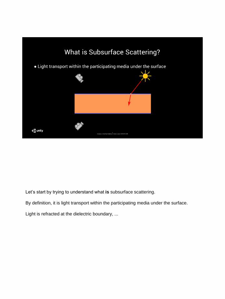
Let’s start by trying to understand what is subsurface scattering.

By definition, it is light transport within the participating media under the surface.

Light is refracted at the dielectric boundary, ...

... scattered within the participating media multiple times, ...

... and refracted outside again.

Scattering is typically assumed to be isotropic (which is a reasonable assumption for

multiple scattering), and is therefore modelled with a radially symmetric diffusion

profile [Jensen 2001].

This leads us to the following definition of the bidirectional subsurface scattering

reflectance distribution function (or BSSRDF for short), where R is the diffusion

profile, F_t is Fresnel transmission and C is the normalization constant.

What this means in practice is that materials such as skin typically look smooth and

organic rather than plasticy. <here is an example of a model showing subsurface

scattering on skin and eyes rendered with HDRP in real-time>

You also get some color bleeding around areas where illumination changes abruptly.

It appears that there’s a certain misconception that with SSS you get pronounced

color bleeding near all shadow boundaries. In fact, it is very subtle if the shadow is

soft.

How is subsurface scattering typically implemented?

The first real-time SSS approach was proposed by Eugene d’Eon, and used a mixture

of Gaussians (4, to be specific) to create a numerical fit for a measured diffusion

profile.

Gaussian was chosen for several reasons:

- A mixture of Gaussians is a convenient target for a numerical fit.

- Additionally, convolution with a Gaussian is separable, and so it has a linear

(rather than quadratic) complexity in the number of samples.

- And finally, repeated convolutions with a “smaller” Gaussian are equivalent to

a single convolution with a “larger” Gaussian.

This approach yields fantastic results, but it is still too expensive for games, even

today. Therefore, real-time constraints force us to implement SSS in the screen

space.

The filter is usually composed of 1 or 2 Gaussians and a Dirac delta function which, in

practice, means that you interpolate between the original and the blurred image.

A single Gaussian does a pretty good job at approximating multiple scattering.

However, even a mix of 2 Gaussians struggles to accurately represent the

combination of single and multiple scattering.

On the image, you can see the reference results in white, and the dual Gaussian

approximation in red.

After implementing the Gaussian mix model, we have encountered another problem -

it is not artist-friendly.

A Gaussian is just a mathematical concept, and it has no physical meaning in the

context of SSS. And when you have two of them with a lerp parameter, that’s 7

degrees of freedom, and it’s not exactly clear how to set them up so that the resulting

combination makes sense.

It is worth noting that a skilled artist can still achieve great results with the Gaussian

mix model. However, this can be a lengthy and complicated process, which is not a

right fit for Unity.

So, is there a better solution? Well, it is in the title of this talk. :-)

We implemented Burley’s normalized diffusion model, which we call the Disney SSS.

It provides an accurate fit for the reference data obtained using Monte Carlo

simulation.

Naturally, that means accounting for both single and multiple scattering.

It has only two parameters: the volume albedo A, and the shape parameter s. Both of

them can be interpreted as colors.

The shape parameter is inversely proportional to the scattering distance, and this is

what we expose in the UI.

If we look at the graph of the resulting profiles, two things become obvious:

1. The sharp peak and the long tail cannot be modeled with a single Gaussian

2. The resulting filter is clearly non-separable

The diffusion profile is normalized, and can be directly used as a probability density

function (or PDF for short). This is a useful property for Monte Carlo integration, as

we’ll see in a bit.

● The diffusion profile is normalized, it can

A diffuse BRDF approximates SSS when the scattering distance is within the footprint

of the pixel.

What this means is that both shading models should have the same visuals past a

certain distance.

In order to achieve that, we use the formulation of the Disney Diffuse BRDF to define

the diffuse transmission behavior at the dielectric boundary.

While it doesn’t match transmission defined by the GGX model, it’s still better than

assuming a Lambertian distribution.

We do not model specular transmission, and our model does not generalize to low-

albedo materials like glass.

Note: transmission may be a confusing term. Specular transmission refers to the

Fresnel transmission at a smooth dielectric boundary.

Diffuse transmission models transmission through a rough dielectric boundary, and

typically assumes a high amount of multiple scattering. Often, it’s just the Lambertian

term.

To enforce visual consistency, we also directly use the surface albedo as the volume

albedo.

We offer 2 albedo texturing options:

1. Post-scatter texturing should be used when the albedo texture already

contains some color bleed due to SSS. That is the case for scans and

photographs. In this mode, we only apply the albedo once, at the exit location.

2. Pre- and post-scatter texturing effectively blurs the albedo, which can result in

a softer, more natural look, which is desirable in certain cases.

Let’s look at some examples of both texturing modes.

We’ll start with the original model of Emily kindly shared by the WikiHuman project.

This picture clearly needs some SSS...

So here it is, with post-scatter texturing enabled.

(flip back and forth)

You may notice that the post-scatter option does a better job at preserving detail, as

expected.

The difference is subtle, so I encourage you to look at the slides on a good display

later.

And for comparison, this is pre- and post-scatter.

(flip back and forth)

You may notice that the post-scatter option does a better job at preserving detail, as

expected.

The difference is subtle, so I encourage you to look at the slides on a good display

later.

Since Burley’s diffusion profiles are normalized, SSS can be implemented as an

energy-conserving blur filter.

You can imagine light energy being redistributed from the point of entry across the

surrounding surface...

Similarly to the previous approaches, we perform convolution in the screen space,

and use the depth buffer to account for the surface geometry.

Let’s have a visual overview of the entire algorithm.

Lighting pass:

Compute incident radiance at the entry point of the surface

Perform diffuse transmission from the light direction into the surface

Apply the entry point albedo depending on the texturing mode

Record transmitted radiance in a render target

SSS pass:

Perform bilateral filtering of the radiance buffer with the diffusion profile around the

exit point

Apply the exit point albedo depending on the texturing mode

Perform diffuse transmission outside of the surface in the view direction

Ideally, we should directly sample the surface of the object*, but that is too expensive

for real-time applications.

Instead, we use a set of samples which we precompute offline, and (conceptually)

place them on a disk, pictured here with a dashed green line.

As the picture demonstrates, this planar approximation is not necessarily a good

match for the shape of the surface.

What’s arguably worse, since projection of samples from the disk onto the surface

distorts distances, projected samples end up within a different distribution. We’ll have

to do something about that, but first…

Note: that’s basically SSS using photon mapping.

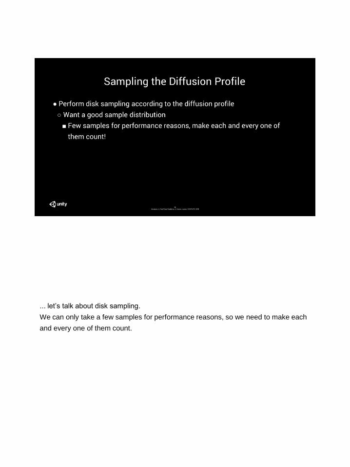
... let’s talk about disk sampling.

We can only take a few samples for performance reasons, so we need to make each

and every one of them count.

Therefore, we importance sample radial distances - we distribute them according to

the PDF of the diffusion profile.

The shape parameter s is a spectral value, and it is inversely proportional to the

scattering distance, which itself is proportional to variance.

Since we want to achieve the best possible variance reduction, we choose to

importance sample the color channel which corresponds to the largest scattering

distance (for skin, it is the red channel).

For importance sampling, it is necessary to invert the cumulative distribution function

(or CDF for short).

Unfortunately, the CDF is not analytically invertible, so we resort to numerical

inversion using Halley’s method, which is, nonetheless, quite efficient in practice.

Note: Halley’s method is the second algorithm in the class of Householder's methods,

after Newton's method.

Finally, we use the Fibonacci sequence to uniformly sample the polar angle. It yields

a good sample distribution on spheres and disks, and is useful in many contexts,

such as reflection probe filtering.

We use the Monte Carlo integration method to perform convolution across the disk. It

simply boils down to the dot product of sample values and weights.

The importance sampling process results in a precomputed sample pattern which can

look like this.

Notice that we sample more densely near the origin since most of the energy is

concentrated there.

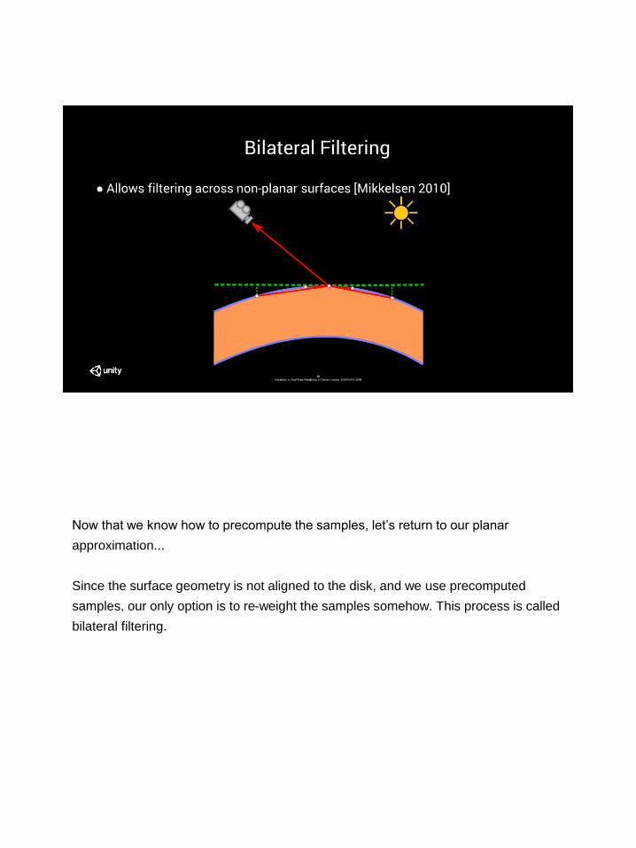
Now that we know how to precompute the samples, let’s return to our planar

approximation...

Since the surface geometry is not aligned to the disk, and we use precomputed

samples, our only option is to re-weight the samples somehow. This process is called

bilateral filtering.

Bilateral filtering makes convolution take depth into account.

Getting this right is very important, not just for a quality boost, but also to avoid the

background bleeding onto the foreground, and vice versa.

Using the Monte Carlo formulation of convolution, sample weights are defined as the

ratio between the value of the function and the PDF.

Modifying the value of the function is easy - we just evaluate the profile using the

actual Euclidean distance between the entry and the exit points.

Note: for the ease of exposition, the math assumes a right triangle and thus uses the

Pythagorean theorem. Generally speaking, you should account for the perspective

distortion as well [Mikkelsen 2010].

Unfortunately, we cannot do the same for the PDF, since our sample positions are

already distributed according to this old “planar” PDF.

If we make a connection between the formula for Monte Carlo integration and the

quadrature formula for integration over area, we can see that the PDF value is

inversely proportional to the area associated with each sample.

But how do you compute this area? It’s possible to make certain assumptions about

the surface and add some cosine factors to account for slopes...

However, solving this problem in a general and robust way is hard, especially due to

the limited information in the screen space.

Instead, we can simply utilize the fact that our filter is meant to be energy conserving,

and normalize the weights to sum up to 1.

Now that we know how to perform bilateral filtering across the disk, let’s consider how

to place and orient this disk.

The disk is naturally placed at the intersection of the camera ray with the geometry, in

the world or the camera space.

But what about the orientation of the disk? We have several options.

The 0 order approximation is to align the disk parallel to the screen plane, which

directly corresponds to a disk in the screen space.

It’s simple and fast, but can result in poor sample distribution for geometry at oblique

angles.

A better solution is to align the disk with the tangent plane of the neighbourhood of the

surface point (1st order approximation).

This can be challenging because the G-Buffer typically does not contain the

interpolated vertex normal.

And, unfortunately, using the shading normal can result in artifacts, as it often has

little in common with the geometry around the surface point, and can even be back-

facing.

It’s worth noting that even the naive method performs quite well in practice.

SSS is also responsible for the translucent look of back-lit objects.

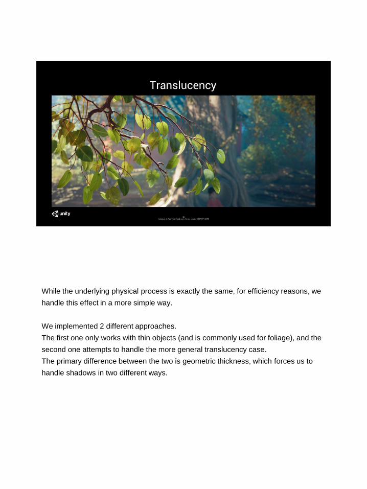
While the underlying physical process is exactly the same, for efficiency reasons, we

handle this effect in a more simple way.

We implemented 2 different approaches.

The first one only works with thin objects (and is commonly used for foliage), and the

second one attempts to handle the more general translucency case.

The primary difference between the two is geometric thickness, which forces us to

handle shadows in two different ways.

For thin object translucency, we use the simple model proposed by Jorge Jimenez.

We assume that for the current pixel, the geometry is a planar slab of constant

thickness with the back-face normal being the reversed front-face normal.

Thickness is provided in an artist-authored texture map.

Additionally, we assume that the entire back face receives constant illumination.

As geometry itself is thin, shadowing is the same for the front and the back faces, so

we can share a single shadow map fetch.

Given this simplified setup, it’s possible to analytically integrate the contribution of the

diffusion profile over the back face.

And as before, we transmit twice and apply the albedo of the front face.

For thicker objects, reusing the shadowing status of the front face obviously does not

work (since the back face may shadow the front face).

Initially, we attempted to compute thickness at runtime solely using the distance to the

closest occluder given by the shadow map.

It quickly became apparent that this approach does not work well for fine geometric

features due to the limited precision of shadow maps.

Instead, we opted for a combined approach. We compute thickness using both

methods, and take the maximum value, which gives an artist an opportunity to work

around shadow mapping issues using the “baked” thickness texture.

The method admittedly requires some tweaking, but with some effort it is possible to

achieve plausible results.

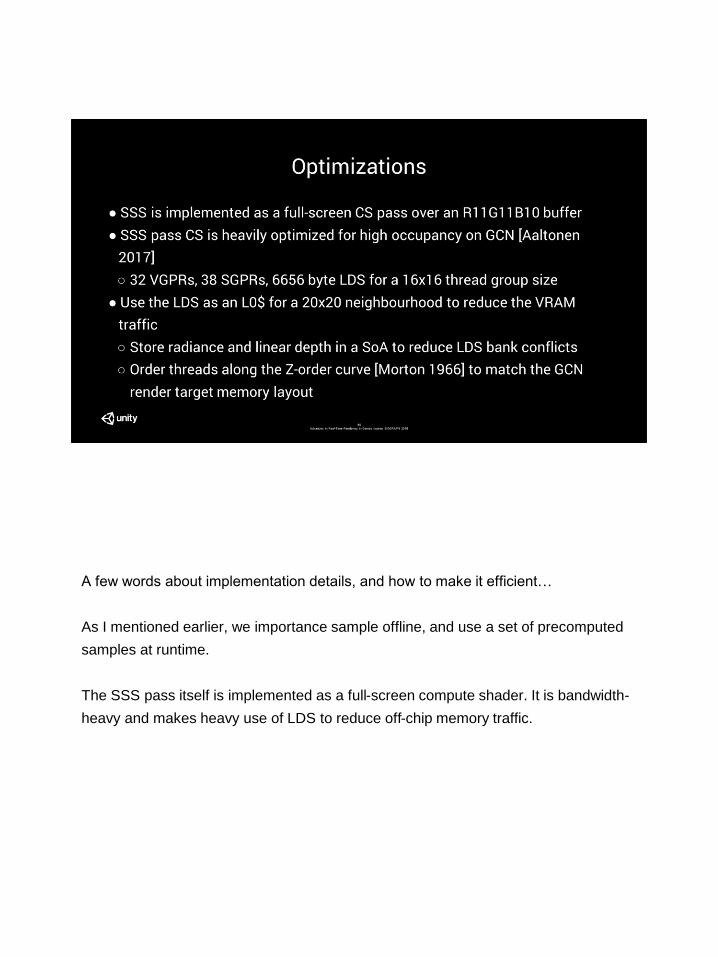
A few words about implementation details, and how to make it efficient…

As I mentioned earlier, we importance sample offline, and use a set of precomputed

samples at runtime.

The SSS pass itself is implemented as a full-screen compute shader. It is bandwidth-

heavy and makes heavy use of LDS to reduce off-chip memory traffic.

The thread group (shown as numbers) is composed of 4 wavefronts, with individual

threads ordered along the Z-order curve for improved data locality.

The LDS cache (shown as color blocks) contains radiance and linear depth values,

and has a 2 texel border so that each pixel has at least a small cached

neighbourhood.

We tag the stencil with the material type during the G-Buffer pass. This allows us to

create a hierarchical stencil representation, and discard whole pixel tiles during the

SSS pass.

During the lighting pass, we also tag the subsurface lighting buffer in order to avoid

performing per-pixel stencil test during the SSS pass.

We also evaluate both transmission events during the lighting pass. While this is

conceptually wrong, the visual difference is very small, and it allows us to avoid

reading the normal buffer during the SSS pass.

We also implemented a basic LOD system.

We change the number of samples depending on the screen-space footprint of the

filter in 3 discrete steps: we disable filtering for sub-pixel sized disks, we use 21

samples for medium sizes, and 55 otherwise.

Visuals remain consistent, and LOD transitions are invisible.

We also found it important to perform random per-pixel rotations of the sample

distribution. This allows us to trade structured undersampling artifacts for less

objectionable noise.

On PS4, we restrict ourselves to 21 samples per pixel.

With the setup you see on the screen, the compute shader which performs

convolution and merges diffuse and specular lighting buffers takes 1.16 milliseconds

to execute.

We also implemented the latest Gaussian mix model of Jorge Jimenez for

comparison.

If you can see the difference, you don’t need glasses. :-)

*flip back and forth*

With a single parameter, the Disney model is very easy to control, and it’s possible to

achieve good results in a matter of minutes.

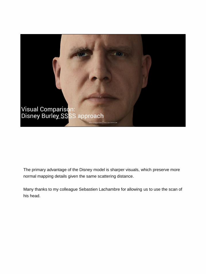
The primary advantage of the Disney model is sharper visuals, which preserve more

normal mapping details given the same scattering distance.

Many thanks to my colleague Sebastien Lachambre for allowing us to use the scan of

his head.

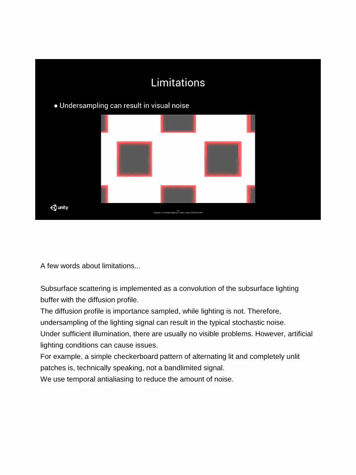
A few words about limitations...

Subsurface scattering is implemented as a convolution of the subsurface lighting

buffer with the diffusion profile.

The diffusion profile is importance sampled, while lighting is not. Therefore,

undersampling of the lighting signal can result in the typical stochastic noise.

Under sufficient illumination, there are usually no visible problems. However, artificial

lighting conditions can cause issues.

For example, a simple checkerboard pattern of alternating lit and completely unlit

patches is, technically speaking, not a bandlimited signal.

We use temporal antialiasing to reduce the amount of noise.

Another limitation of our method is kernels with very large screen footprint. Samples

end up being very far apart, trashing the texture cache and degrading performance.

Finally, thick object translucency makes too many assumptions to produce accurate

results for complex thick objects.

In the future, we would like to extend our implementation to properly support tangent-

space integration.

Since interpolated vertex normals are not available in the G-Buffer, our plan is to

compute a robust tangent space normal from the depth buffer.

For translucency, we would like to go beyond the current “constant thickness

uniformly lit slab” model.

This requires diffuse shading of the closest back face, and another screen-space

pass to integrate it with front-face SSS.

Thank you.

hello again, and thanks for sticking around. i will give

Documents