heikki orsila - tuni · form capabilities and required functionality. a point x is selected from...
TRANSCRIPT


Tampereen teknillinen yliopisto. Julkaisu 972 Tampere University of Technology. Publication 972 Heikki Orsila Optimizing Algorithms for Task Graph Mapping on Multiprocessor System on Chip Thesis for the degree of Doctor of Science in Technology to be presented with due permission for public examination and criticism in Tietotalo Building, Auditorium TB111, at Tampere University of Technology, on the 17th of June 2011, at 12 noon. Tampereen teknillinen yliopisto - Tampere University of Technology Tampere 2011

ISBN 978-952-15-2585-8 (printed) ISBN 978-952-15-2590-2 (PDF) ISSN 1459-2045

ABSTRACT
The objective of this Thesis is to analyze and improve MPSoC design space explo-ration, specifically the task mapping using Simulated Annealing (SA) with fully auto-matic optimization. The work concentrates mostly on application execution time op-timization. However, a trade-off between memory buffer and time optimization anda trade-off between power and time optimization is also analyzed. Applications arerepresented as public Standard Task Graph sets and Kahn Process Networks (KPNs).
Main focus is on SA as the optimization algorithm for task mapping. A state of theart survey is presented on using SA for task mapping. Thesis analyzes the impact ofSA parameters on convergence. A systematic method is presented for automaticallyselecting parameters. The method scales up with respect to increasing HW and SWcomplexity. It is called Simulated Annealing with Automatic Temperature (SA+AT).
Optimal subset mapping (OSM) algorithm is presented as a rapidly converging taskmapping algorithm. SA+AT is compared with OSM, Group Migration, RandomMapping and a Genetic Algorithm. SA+AT gives the best results. OSM is the mostefficient algorithm.
Thesis presents new data on the convergence of annealing. Answers are given toglobal optimum convergence properties and the convergence speed in terms of map-ping iterations. This covers optimization of the run-time of mapping algorithms sothat a trade-off can be made between solution quality and algorithm’s execution time.SA+AT saves up to half the optimization time without significantly decreasing solu-tion quality.
Recommendations are presented for using SA in task mapping. The work is intendedto help other works to use SA. DCS task mapper, an open source simulator andoptimization program, is presented and published to help development and evaluationof mapping algorithms. The data to reproduce Thesis experiments with the programis also published.

ii Abstract

PREFACE
The work presented in this Thesis has been carried out in the Department of ComputerSystems at Tampere University of Technology during the years 2003-2011.
I thank my supervisor Prof. Timo D Hamalainen for guiding and encouraging metowards doctoral degree. Grateful acknowledgments go also to Prof. Andy Pimenteland Adj. Prof. Juha Plosila for thorough reviews and constructive comments on themanuscript.
It has been my pleasure to work in the Department of Computer Systems. Manythanks to all my colleagues for the discussions and good atmosphere. Especially Dr.Erno Salminen, Dr. Kimmo Kuusilinna, Prof. Marko Hannikainen and Dr. Tero Kan-gas, deserve a big hand for helping me in several matters. In addition, I would liketo thank all the other co-authors and colleagues, Tero Arpinen, M.Sc. Kalle Holma,M.Sc., Tero Huttunen, M.Sc., Dr. Ari Kulmala, Janne Kulmala, Petri Pesonen, M.Sc.,and Riku Uusikartano, M.Sc., with whom I have had pleasant and stimulating discus-sions on and off-topic.
I want to thank my parents for the support they have given me. I also want to thankSusanna for love and understanding.
Tampere, Apr 2011Heikki Orsila

iv Preface

TABLE OF CONTENTS
Abstract . . . . . . . . . . . . . . . . . . . . . . . . . . . . . . . . . . . . i
Preface . . . . . . . . . . . . . . . . . . . . . . . . . . . . . . . . . . . . . iii
Table of Contents . . . . . . . . . . . . . . . . . . . . . . . . . . . . . . . v
List of Publications . . . . . . . . . . . . . . . . . . . . . . . . . . . . . . ix
List of Figures . . . . . . . . . . . . . . . . . . . . . . . . . . . . . . . . . xi
List of Tables . . . . . . . . . . . . . . . . . . . . . . . . . . . . . . . . . xiii
List of abbreviations . . . . . . . . . . . . . . . . . . . . . . . . . . . . . . xvii
1. Introduction . . . . . . . . . . . . . . . . . . . . . . . . . . . . . . . . 1
1.1 MPSoC Design Flow . . . . . . . . . . . . . . . . . . . . . . . . . 1
1.2 The mapping problem . . . . . . . . . . . . . . . . . . . . . . . . . 3
1.3 Objectives and scope of research . . . . . . . . . . . . . . . . . . . 6
1.4 Summary of contributions . . . . . . . . . . . . . . . . . . . . . . 7
1.4.1 Author’s contribution to published work . . . . . . . . . . . 8
1.5 Outline of Thesis . . . . . . . . . . . . . . . . . . . . . . . . . . . 9
2. Design space exploration . . . . . . . . . . . . . . . . . . . . . . . . . . 11
2.1 Overview . . . . . . . . . . . . . . . . . . . . . . . . . . . . . . . 11
2.2 Design evaluation . . . . . . . . . . . . . . . . . . . . . . . . . . . 12
2.3 Design flow . . . . . . . . . . . . . . . . . . . . . . . . . . . . . . 13
2.3.1 Koski Design Flow . . . . . . . . . . . . . . . . . . . . . . 14

vi Table of Contents
3. Related work . . . . . . . . . . . . . . . . . . . . . . . . . . . . . . . . 19
3.1 Simulated Annealing algorithm . . . . . . . . . . . . . . . . . . . . 19
3.2 SA in task mapping . . . . . . . . . . . . . . . . . . . . . . . . . . 20
3.3 SA parameters . . . . . . . . . . . . . . . . . . . . . . . . . . . . . 24
3.3.1 Move functions . . . . . . . . . . . . . . . . . . . . . . . . 25
3.3.2 Acceptance functions . . . . . . . . . . . . . . . . . . . . . 27
3.3.3 Annealing schedule . . . . . . . . . . . . . . . . . . . . . . 27
4. Publications . . . . . . . . . . . . . . . . . . . . . . . . . . . . . . . . 31
4.1 Problem space for Publications . . . . . . . . . . . . . . . . . . . . 31
4.2 Research questions . . . . . . . . . . . . . . . . . . . . . . . . . . 32
4.3 Hybrid Algorithm for Mapping Static Task Graphs on MultiprocessorSoCs . . . . . . . . . . . . . . . . . . . . . . . . . . . . . . . . . . 34
4.4 Parameterizing Simulated Annealing for Distributing Task Graphs onmultiprocessor SoCs . . . . . . . . . . . . . . . . . . . . . . . . . 35
4.5 Automated Memory-Aware Application Distribution for Multi-ProcessorSystem-On-Chips . . . . . . . . . . . . . . . . . . . . . . . . . . . 36
4.6 Optimal Subset Mapping And Convergence Evaluation of MappingAlgorithms for Distributing Task Graphs on Multiprocessor SoC . . 37
4.7 Evaluating of Heterogeneous Multiprocessor Architectures by En-ergy and Performance Optimization . . . . . . . . . . . . . . . . . 38
4.8 Best Practices for Simulated Annealing in Multiprocessor Task Dis-tribution Problems . . . . . . . . . . . . . . . . . . . . . . . . . . 39
4.9 Parameterizing Simulated Annealing for Distributing Kahn ProcessNetworks on Multiprocessor SoCs . . . . . . . . . . . . . . . . . . 40
4.9.1 Corrected and extended results . . . . . . . . . . . . . . . . 40
5. DCS task mapper . . . . . . . . . . . . . . . . . . . . . . . . . . . . . 47
5.1 DCS task mapper . . . . . . . . . . . . . . . . . . . . . . . . . . . 47
5.2 Job clustering with jobqueue . . . . . . . . . . . . . . . . . . . . . 49

Table of Contents vii
6. Simulated Annealing convergence . . . . . . . . . . . . . . . . . . . . . 53
6.1 On global optimum results . . . . . . . . . . . . . . . . . . . . . . 53
6.2 On SA acceptance probability . . . . . . . . . . . . . . . . . . . . 60
6.2.1 On acceptor functions . . . . . . . . . . . . . . . . . . . . 60
6.2.2 On zero transition probability . . . . . . . . . . . . . . . . 63
6.3 On Comparing SA+AT to GA . . . . . . . . . . . . . . . . . . . . 63
6.3.1 GA heuristics . . . . . . . . . . . . . . . . . . . . . . . . . 63
6.3.2 Free parameters of GA . . . . . . . . . . . . . . . . . . . . 66
6.3.3 GA experiment . . . . . . . . . . . . . . . . . . . . . . . . 67
7. Recommendations for using Simulated Annealing . . . . . . . . . . . . . 73
7.1 On publishing results for task mapping with Simulated Annealing . 73
7.2 Recommended practices for task mapping with Simulated Annealing 74
8. On relevance of the Thesis . . . . . . . . . . . . . . . . . . . . . . . . . 77
9. Conclusions . . . . . . . . . . . . . . . . . . . . . . . . . . . . . . . . 81
9.1 Main results . . . . . . . . . . . . . . . . . . . . . . . . . . . . . . 81
Bibliography . . . . . . . . . . . . . . . . . . . . . . . . . . . . . . . . . . 85
Publication 1 . . . . . . . . . . . . . . . . . . . . . . . . . . . . . . . . . . 97
Publication 2 . . . . . . . . . . . . . . . . . . . . . . . . . . . . . . . . . . 103
Publication 3 . . . . . . . . . . . . . . . . . . . . . . . . . . . . . . . . . . 109
Publication 4 . . . . . . . . . . . . . . . . . . . . . . . . . . . . . . . . . . 131
Publication 5 . . . . . . . . . . . . . . . . . . . . . . . . . . . . . . . . . . 139
Publication 6 . . . . . . . . . . . . . . . . . . . . . . . . . . . . . . . . . . 147
Publication 7 . . . . . . . . . . . . . . . . . . . . . . . . . . . . . . . . . . 171

viii Table of Contents

LIST OF PUBLICATIONS
This Thesis is based on the following publications: [P1]-[P7]. The Thesis also con-tains some unpublished material.
[P1] H. Orsila, T. Kangas, T. D. Hamalainen, Hybrid Algorithm for MappingStatic Task Graphs on Multiprocessor SoCs, International Symposium onSystem-on-Chip (SoC 2005), pp. 146-150, 2005.
[P2] H. Orsila, T. Kangas, E. Salminen, T. D. Hamalainen, Parameterizing Simu-lated Annealing for Distributing Task Graphs on multiprocessor SoCs, Inter-national Symposium on System-on-Chip, pp. 73-76, Tampere, Finland, Nov14-16, 2006.
[P3] H. Orsila, T. Kangas, E. Salminen, M. Hannikainen, T. D. Hamalainen, Auto-mated Memory-Aware Application Distribution for Multi-Processor System-On-Chips, Journal of Systems Architecture, Volume 53, Issue 11, ISSN 1383-7621, pp. 795-815, 2007.
[P4] H. Orsila, E. Salminen, M. Hannikainen, T.D. Hamalainen, Optimal Sub-set Mapping And Convergence Evaluation of Mapping Algorithms for Dis-tributing Task Graphs on Multiprocessor SoC, International Symposium onSystem-on-Chip, Tampere, Finland, 2007, pp. 52-57.
[P5] H. Orsila, E. Salminen, M. Hannikainen, T.D. Hamalainen, Evaluation ofHeterogeneous Multiprocessor Architectures by Energy and Performance Op-timization, International Symposium on System-on-Chip 2008, pp. 157-162,Tampere, Finland, Nov 4-6, 2008.
[P6] H. Orsila, E. Salminen, T. D. Hamalainen, Best Practices for Simulated An-nealing in Multiprocessor Task Distribution Problems, Chapter 16 of the

x List of Publications
Book “Simulated Annealing”, ISBN 978-953-7619-07-7, I-Tech Educationand Publishing KG, pp. 321-342, 2008.
[P7] H. Orsila, E. Salminen, T. D. Hamalainen, Parameterizing Simulated An-nealing for Distributing Kahn Process Networks on Multiprocessor SoCs,International Symposium on System-on-Chip 2009, Tampere, Finland, Oct5-7, 2009.

LIST OF FIGURES
1 Koski design flow for multiprocessor SoCs [38] . . . . . . . . . . . 2
2 MPSoC implementation starts from the problem space that has plat-form capabilities and required functionality. A point x is selectedfrom the problem space X . The point x defines a system which is im-plemented and evaluated with respect to measures in objective spaceY . These measures include performance, power, silicon area and cost.Objective space measures define the objective function value f (x),which is the fitness of the system. . . . . . . . . . . . . . . . . . . 3
3 The mapping process. Boxes indicate data and ellipses are operations. 4
4 SW components (application tasks) are mapped to HW components.T denotes an application task. PE denotes a processing element. . . 4
5 Evaluation of several mapping algorithms. Number of iterations andthe resulting application speedup are compared for each algorithm. . 12
6 Koski design flow from code generation to physical implementation[38] . . . . . . . . . . . . . . . . . . . . . . . . . . . . . . . . . . 15
7 Video encoder modelled as a KPN [65] . . . . . . . . . . . . . . . 16
8 Two phase exploration method [38] . . . . . . . . . . . . . . . . . 17
9 Static exploration method [38] . . . . . . . . . . . . . . . . . . . . 17
10 Pseudocode of the Simulated Annealing (SA) algorithm . . . . . . . 20
11 DCS task mapper data flow and state transitions. Solid line indicatesdata flow. Dashed line indicates causality between events in the statemachine. . . . . . . . . . . . . . . . . . . . . . . . . . . . . . . . . 48

xii List of Figures
12 SA+AT convergence with respect to global optimum with L= 16,32,64,128and 256 for 32 nodes. SA+AT chooses L = 32. Lines show propor-tion of SA+AT runs that converged within p from global optimumfor a given value of L. Lower p value on X-axis is better. Higherprobability on Y-axis is better. . . . . . . . . . . . . . . . . . . . . 57
13 Expected number of iterations to reach global optimum within p =
0%,2%,5% and 10% for L = 16,32,64,128 and 256 with 32 nodes.SA+AT chooses L = 32. Lower p value on X-axis is better. Lowernumber of iterations on Y-axis is better. . . . . . . . . . . . . . . . 58
14 Task graph execution time for one graph plotted against the num-ber of mappings. All possible mapping combinations for 32 nodesand 2 PEs were computed with brute force search. One node map-ping was fixed. 31 node mappings were varied resulting into 231 =
2147483648 mappings. The initial execution time is 875 µs, mean1033 µs and standard deviation 113 µs. There is only one mappingthat reaches the global optimum 535 µs. . . . . . . . . . . . . . . . 59
15 Pseudocode of a Genetic Algorithm (GA) heuristics . . . . . . . . . 64
16 Distribution of parameter costs in the exploration process. Y-axis isthe mean of normalized costs, 1.00 being the global optimum. Value1.1 would indicate that a parameter was found that converges on av-erage within 10% of the global optimum. Lower value is better. . . . 67
17 Expected number of iterations to reach global optimum within p =
0%,2%,5% and 10% for GA and SA. Lower p value on X-axis isbetter. Lower number of iterations on Y-axis is better. . . . . . . . 71

LIST OF TABLES
1 Table of publications and problems where Simulated Annealing isapplied. Task mapping with SA is applied in a publication when“Mapping sel.” column is “Y”. Task scheduling and communica-tion routing with SA is indicated similarly with “Sched. sel.” and“Comm. sel.” columns, respectively. All 14 publications apply SAto task mapping in this survey, five to task scheduling, and one tocommunication routing. . . . . . . . . . . . . . . . . . . . . . . . 21
2 Simulated Annealing move heuristics and acceptance functions. “Movefunc.” indicates the move function used for SA. “Acc. func” indi-cates the acceptance probability function. “Ann sch.” indicates theannealing schedule. “q” is the temperature scaling co-efficient forgeometric annealing schedules. “T0 ada.” means adaptive initial tem-perature selection. “Stop ada.” means adaptive stopping criteria foroptimization. “L” is the number of iterations per temperature level,where N is the number of tasks and M is the number of PEs. . . . . 25
3 Scope of publications based on optimization criteria and researchquestions . . . . . . . . . . . . . . . . . . . . . . . . . . . . . . . 32
4 Automatic and static temperature compared: SA+AT vs SA+ST speedupvalues with setup A. Higher value is better. . . . . . . . . . . . . . . 42
5 Automatic and static temperature compared: SA+AT vs SA+ST num-ber of mappings with setup A. Lower value is better. . . . . . . . . 42
6 Brute force vs. SA+AT with setup A for 16 node graphs. Proportionof SA+AT runs that converged within p from global optimum. Higherconvergence proportion value is better. Lower number of mappingsis better. . . . . . . . . . . . . . . . . . . . . . . . . . . . . . . . . 43

xiv List of Tables
7 Brute force vs. SA+AT with setup B for 16 node graphs. Proportionof SA+AT runs that converged within p from global optimum. Higherconvergence proportion value is better. Lower number of mappingsis better. . . . . . . . . . . . . . . . . . . . . . . . . . . . . . . . . 44
8 Brute force vs. SA+AT with setup A for 16 node graphs: Approxi-mate number of mappings to reach within p percent of global opti-mum. As a comparison to SA+AT, Brute force takes 32770 mappingsfor 2 PEs, 14.3M mappings for 3 PEs and 1.1G mappings for 4 PEs.Lower value is better. . . . . . . . . . . . . . . . . . . . . . . . . . 45
9 Brute force vs. SA+AT with setup B for 16 node graphs: Approxi-mate number of mappings to reach within p percent of global opti-mum. As a comparison to SA+AT, Brute force takes 32770 mappingsfor 2 PEs, 14.3M mappings for 3 PEs and 1.1G mappings for 4 PEs.Lower value is better. . . . . . . . . . . . . . . . . . . . . . . . . . 46
10 Number of mappings explored, the mapping speed and the time com-puted with DCS task mapper for publications . . . . . . . . . . . . 50
11 SA+AT convergence with respect to global optimum with L= 16,32,64,128and 256 for 32 nodes. Automatic parameter selection method inSA+AT chooses L = 32. Values in table show proportion of SA+ATruns that converged within p from global optimum. Higher value isbetter. . . . . . . . . . . . . . . . . . . . . . . . . . . . . . . . . . 55
12 Approximate expected number of mappings for SA+AT to obtainglobal optimum within p percent for L = 16,32,64,128 and 256 for32 nodes. SA+AT chooses L = 32. Best values are in boldface oneach row. Lower value is better. . . . . . . . . . . . . . . . . . . . 56
13 Proportion of SA runs that converged within p percent of global opti-mum and the associated number of mappings within that range com-puted from the brute force search. Higher mapping number and SArun proportion is better. . . . . . . . . . . . . . . . . . . . . . . . . 58

List of Tables xv
14 Global optimum convergence rate varies between graphs and L val-ues. The sample is 10 graphs. Columns show the minimum, mean,median and maximum probability of convergence to global optimum,respectively. Value 0% in Min column means there was a graph forwhich global optimum was not found in 1000 SA+AT runs. ForL ≥ 32 global optimum was found for each graph. Note, the Meancolumn has same values as the p = 0% row in Table 11. . . . . . . 60
15 Comparing average and median gain values for the inverse exponen-tial and exponential acceptors. A is the mean gain for experimentsrun with inverse exponential acceptor. B is the same for exponentialacceptor. C and D are median gain values for inverse exponential ac-ceptor and exponential acceptor, respectively. Higher value is betterin columns A, B, C and D. . . . . . . . . . . . . . . . . . . . . . . . 61
16 Comparing average and median iterations for the inverse exponentialand exponential acceptors. E is the mean iterations for experimentsrun with inverse exponential acceptor. F is the same for exponentialacceptor. G and H are the median iterations for inverse exponen-tial and exponential acceptors, respectively. Lower value is better incolumns E, F , G and H. . . . . . . . . . . . . . . . . . . . . . . . 61
17 The table shows difference between SA+AT convergence rate of nor-malized exponential acceptor and normalized inverse exponential ac-ceptor results. Inverse exponential acceptor results are shown in Ta-ble 11. The experiment is identical to that in Table 11. Automaticparameter selection method in SA+AT chooses L = 32. p percent-age shows the convergence within global optimum. A positive valueindicates normalized exponential acceptor is better. . . . . . . . . . 62
18 The best found GA parameters for different max iteration counts imax.Discrimination and elitism presented as the number of members in apopulation. . . . . . . . . . . . . . . . . . . . . . . . . . . . . . . 68

xvi List of Tables
19 SA+AT and GA convergence compared with respect to global op-timum. Automatic parameter selection method in SA+AT choosesL = 32. Mean mappings per run for GA is the imax value. Values intable show proportion of optimization runs that converged within pfrom global optimum. Higher value is better. . . . . . . . . . . . . 69
20 Approximate expected number of mappings for SA+AT and GA toobtain objective value within p percent of the global optimum. SA+ATchooses L = 32 by default. Best values are in boldface on each row.Lower value is better. . . . . . . . . . . . . . . . . . . . . . . . . . 70
21 Table of citations to the publications in this Thesis. “Citations” col-umn indicates publications that refer to the given paper on the “Pub-lication” column. Third column indicates which of these papers useor apply a method presented in the paper. The method may be usedin a modified form. . . . . . . . . . . . . . . . . . . . . . . . . . . 77

LIST OF ABBREVIATIONS
ACO Ant Colony Optimization
CP Critical Path
CPU Central Processing Unit
DA Decomposition Approach (constraint programming)
DAG Directed Acyclic Graph
DLS Dynamic Level Scheduling
DMA Direct memory access
DSE Design Space Exploration
DSP Digital Signal Processing
FIFO First In First Out
FP Fast pre-mapping
FSM Finite State Machine
GA Genetic Algorithm
GM Group Migration
GPU Graphics Processing Unit
GSA Genetic Simulated Annealing
HA Hybrid Algorithm
HTG Hierarchical Task Graph
xviii List of abbreviations
HW Hardware
iff If and only if
ISS Instruction Set Simulator
KPN Kahn Process Network
LIFO Last In First Out (stack)
LP Linear Programming
LS Local Search
MoC Model of Computation
MPSoC Multiprocessor System-on-Chip
OSM Optimal Subset Mapping
PE Processing Element (CPU, acceleration unit, etc.)
PIO Programmed IO; Processor is directly involved with IO ratherthan DMA controller.
ReCA Reference Constructive Algorithm
RM Random Mapping
SA Simulated Annealing
SA+AT Simulated Annealing with Automatic Temperature
SoC System-on-Chip
ST Single task move heuristics
STG Static Task Graph
SW Software
TS Tabu Search

1. INTRODUCTION
A multiprocessor system-on-chip (MPSoC) consists of processors, memories, accel-erators and interconnects. Examples include the Cell, TI OMAP, ST Nomadik SA [87],HIBI [47] [54] [66]. MPSoC design requires design space exploration (DSE) [30] tofind an appropriate system meeting several requirements that may be mutually con-flicting, e.g. energy-efficiency, cost and performance.
An MPSoC may contain tens of processing elements (PEs) and thousands of softwarecomponents. Implementing the SoC and applications requires many person-years ofwork. The complexity of the system requires high-level planning, feasibility estima-tion and design to meet the requirements and reduce the risk of the project.
1.1 MPSoC Design Flow
High-level SoC design flows are used to decrease the investment risk in develop-ment. Figure 1 shows the Koski [39] design flow for MPSoCs at a high level as arepresentative design flow.
The first design phase defines the abstractions and functional components of the sys-tem. UML is used to model the system components. Y-model [41] [42] is applied onthe system being designed. Architecture and applications are modeled separately butcombined together into a system by mapping.
A functional model of the system is created in the second phase. Application code iswritten, or generated if possible, and functionally verified. Performance of applica-tion components are estimated by using benchmarks, test vectors and profiling. Partsof the application may later be implemented in HW to optimize performance.
The third and fourth design phase contains the design space exploration part. Problemspace defines the system parameters being searched for in exploration. This includes

2 1. Introduction
Staticarchitecture exploration
Functional simulation (C/C++)- accurate application model (EFSM)- no platf orm model
Sy stem f unctionality v erif ication
Phy sical implementation
Dy namic architecture exploration
Static task graph analy sis (C)- abstract application model (external behav ior of
application tasks)- abstract platf orm model (parameters)
Conducted analysis and utilized modelsObjective
• Application code generation• Functional v erif ication and early
perf ormance estimation
• Coarse-grain allocation, mapping, and scheduling
Process network simulation (Sy stemC)- abstract application model- abstract processing element model (parameters)- time accurate network model
• Fine-grain allocation and mapping
• Network optimization
• Implementation generation• Full sy stem v erification with
FPGAs
FPGA execution (C, VHDL)- accurate application model - accurate architecture model- perf ormance measurements
Design phase
2
3
4
5
Sy stemmodeling
(application, platf orm)
1 Model creation (UML)- Y-model f or sy stem- TUT, MARTE prof iles f or UML2.0
• Abstraction• Application and platf orm
structure design
Fig. 1. Koski design flow for multiprocessor SoCs [38]
parameters such as the number of PEs, memory hierarchy, clock frequency, timingevents and placing application tasks to PEs. Objective space determines the proper-ties that are the effects of design choices in the problem space. This includes prop-erties such as execution time, communication time, power and silicon area. Problemspace properties do not directly affect the properties in the objective space. Explo-ration searches for a combination of problem space properties to optimize objectivespace properties. The third and fourth phases differ by the accuracy of objectivespace measures in the simulation model, the fourth is more accurate.
The system is implemented in finer grain with a SystemC model in the fourth designphase. The allocation, schedule and mapping is taken as input from the third phase.The system is optimized again. A significantly fewer number of systems is evaluatedcompare to third phase, because system evaluation is much slower now.
The fifth phase is physical implementation. The system is implemented and veri-fied for FPGA. The application is finalized in C and hardware in VHDL. Accurateobjective space measures are finally obtained.

1.2. The mapping problem 3
MPSoC
System Objective space (Y)
Performance
Power
Silicon area
Cost
f(x)
x
Memory
Processors
Accelerators
Application tasks
Required functionality:
Operating systems
Multiprocessing frameworks
Problem space (X)
Platform capabilities:
Communication network
Fitness
Fig. 2. MPSoC implementation starts from the problem space that has platform capabilitiesand required functionality. A point x is selected from the problem space X. The pointx defines a system which is implemented and evaluated with respect to measures inobjective space Y . These measures include performance, power, silicon area andcost. Objective space measures define the objective function value f (x), which is thefitness of the system.
1.2 The mapping problem
The mapping problem, a part of the exploration process, means finding x ∈ X tooptimize the solution of an objective function f (x)∈Rn, where X is the problem spaceand x is the choice of free design parameters. Objective function uses simulation andestimation techniques to compute objective space (Y ) measures from x. The resultingvalue is a multi-objective optimization problem if n > 1. Figure 2 shows the relationbetween problem and objective space.
Figure 3 shows the mapping process in higher detail. The first stage is system allo-cation where the system is implemented by combining existing components and/orcreating new ones for evaluation. The system is then implemented by mapping se-lected components to HW resources. Figure 4 shows tasks being mapped to PEs andPEs connected with communication network. This yields a system candidate that canbe evaluated. Evaluation part determines objective space measures of the system.Note, the evaluated system may or may not be feasible according to given objectivespace constraints such as execution time, power and area. Pareto optimal feasiblesystems are selected as the output of the process. In single objective case there isonly one such system.

4 1. Introduction
Problem space
(all available HW
and SW components)
Allocation
Selected SW
components
Selected HW
components
Implementation
(mapping, scheduling)
System
candidate
System
evaluation
Objective
measures
feedback
feedback
Fig. 3. The mapping process. Boxes indicate data and ellipses are operations.
T
T
T
T
Communication network
PE PE PE PEHW components
SW components
(application tasks)
Mapping
Fig. 4. SW components (application tasks) are mapped to HW components. T denotes anapplication task. PE denotes a processing element.

1.2. The mapping problem 5
The application consists of tasks that are mapped to PEs. A task is defined to be anyexecutable entity or a specific job that needs to be processed so that the applicationcan serve its purpose. This includes operations such as computing output from input,copying data from one PE to another, mandatory time delay, waiting for an eventto happen. A task has a mapping target, such as PE, task execution priority, execu-tion time slot, communication channel to use, or any discrete value that representsa design choice for a particular task. The mapping target can be determined duringsystem creation or execution time. A number of mappings is evaluated for each sys-tem candidate. The number of mappings depends on the properties of the systemcandidate, including the number of tasks and PEs.
The problem is finding a mapping from N objects to M resources with possible con-straints. This means MN points in the problem space. For example, the problem spacefor 32 tasks mapped to just 2 PEs has 4.3×10⁹ points. It takes 136 years to explorethe whole problem space if evaluating one mapping takes one second. Therefore, itis not possible to explore the whole problem space for anything but small problems.This means the space must be pruned or reduced. A fast optimization procedure isdesired in order to cover a reasonable number of points in the problem space. Thisis the reason for separate third and fourth stages in Koski. However, a fast procedurecomes with the expense of accuracy in objective space measurements, e.g. estimatedexecution time and power.
Several algorithmic approaches have been proposed for task mapping [9] [20]. Themain approaches are non-iterative and iterative heuristics. Non-iterative heuristicscompute a single solution which is not further refined. Simulation is only used forestimating execution times of application tasks and performance of PEs. Tasks aremapped to PEs based on execution time estimates and the structure of the task graph.List scheduling heuristics [51] are often used. Good results from these methods usu-ally require that the critical path of the application is known.
The iterative approaches are often stochastic methods that do random walk in theproblem space. Iterative approaches give better results than non-iterative approachesbecause they can try multiple solutions and use simulations instead of estimates forevaluation. Several iterative algorithms have been proposed for task mapping. Mostof them are based on heuristics such as Simulated Annealing (SA) [12] [44], Ge-netic Algorithms (GA) [31], Tabu Search (TS) [28] [7], local search heuristics, loadbalancing techniques, and Monte Carlo. These methods have also been combined

6 1. Introduction
together. For example, both SA and GA are popular approaches that have been com-bined together into a Genetic Simulated Annealing (GSA) [17] [77].
Parameters of the published algorithms have often not been reported, the effect ofdifferent parameter choices is not analyzed, or the algorithms are too slow. Properparameters vary from task to task, but manual parameter selection is laborious anderror-prone. Therefore, systematic methods and analysis on parameter selection ispreferable in exploration. Development of these methods and analysis is the centralresearch problem in the Thesis. Automatic parameter selection methods are presentedfor SA, and the effects of parameters are analyzed. SA was selected for the Thesisbecause it has been successfully applied on many fields including task mapping, butthere is a lack of information on the effects of SA parameters on task mapping.
1.3 Objectives and scope of research
The objective of this Thesis is to analyze and improve MPSoC design space explo-ration, specifically the task mapping using Simulated Annealing with fully automaticoptimization. The work concentrates mostly on application execution time optimiza-tion. However, [P3] considers a trade-off between memory buffer and time optimiza-tion and [P5] between power and time optimization.
MPSoCs used in this Thesis are modeled on external behavior level. Timings andresource contention is simulated, but actual data is not computed. This allows rapidscheduling, and hence, rapid evaluation of different mappings during the develop-ment work. Applications are represented as public Standard Task Graph sets [81]and Kahn Process Networks (KPNs) [37] generated with kpn-generator [46] withvarying level of optimizing difficulty. The graphs are selected to avoid bias for beingapplication specific, since optimal mapping algorithm depends on the graph topol-ogy and weights for a given application. This Thesis tries to overcome this and findgeneral purpose mapping methods that are suitable to many types of applications.
Main focus is on Simulated Annealing as the optimization algorithm for task map-ping. First, this Thesis analyzes the impact of SA parameters. Many publicationsleave parameter selection unexplained, and often not documented. This harms at-tempts of automatic exploration as manual tuning of parameters is required, whichis also error-prone due to humans. This motivates finding a systematic method for
1.4. Summary of contributions 7
automatically selecting parameters.
Second, Thesis gives answers to global optimum convergence properties and the con-vergence speed in terms of mapping iterations. Optimal solution for the task mappingproblem requires exponential time with respect to number of nodes in the task graph.Spending more iterations to a solve a problem gives diminishing returns. The effec-tiveness of an algorithm usually starts to dampen exponentially after some numberof iterations. These properties have not been examined carefully in task mappingproblems previously.
Third, the Thesis covers optimization of the run-time of mapping algorithms so thata trade-off can be made between solution quality and algorithm’s execution time.
Following research questions are investigated:
1. How to select optimization parameters for a given point in problem space?
2. The convergence rate: How many iterations are needed to reach a given solu-tion quality?
3. How does each parameter of the algorithm affect the convergence rate andquality of solutions?
4. How to speedup the convergence rate? That is, how to decrease the run-timeof mapping algorithm?
5. How often does the algorithm converge to a given solution quality?
1.4 Summary of contributions
Task mapping in design space exploration often lacks systematic method that scaleswith respect to the application and hardware complexity, i.e. the number of task nodesand PEs. This Thesis presents a series of methods how to select parameters for a givenMPSoC. Developed methods are part of the DCS task mapper tool that was usedin Koski design flow [3] [38] [39]. Convergence rate is analyzed for our modifiedSimulated Annealing algorithm. Also, a comparison is made between automaticallyselected parameters and global optimum solutions. We are not aware of a globaloptimum comparison that presents such detailed comparison. Presented methods are

8 1. Introduction
compared to other studies, that specifically use SA or other optimization method.Their advantages and disadvantages are analyzed.
Summary of contributions of this Thesis are:
• Review of existing work on task mapping
• Development of task mapping methods including an automatic parameter se-lection method for Simulated Annealing that scales up with respect to HW andSW complexity. This is called Simulated Annealing with Automatic Tempera-ture (SA+AT).
• Optimal subset mapping (OSM) algorithm
• Comparisons and analyses of developed methods including:
– Comparison of SA, OSM, Group Migration (GM) and Random Mapping(RM) and GA
– Convergence analysis of SA+AT with respect to global optimum solution
– Comparison of SA+AT to published mapping techniques
• Tool development: DCS task mapper tool that is used to explore mapping al-gorithms themselves efficiently
1.4.1 Author’s contribution to published work
The Author is the main author, contributor in all the Publications and the author ofDCS task mapper.
Tero Kangas helped developing ideas in [P1]-[P3].
Erno Salminen helped developing ideas in [P2]-[P7]. In particular, many importantexperiments were proposed by him.
Professor Timo D. Hamalainen provided highly valued insights and comments forthe research and helped to improve text in all the Publications.
Professor Marko Hannikainen helped to improve text in [P3]-[P5].

1.5. Outline of Thesis 9
1.5 Outline of Thesis
Thesis is outlined as follows. Chapter 2 introduces design space exploration and con-cepts relevant to task mapping. Chapter 3 presents related work for task mapping.Chapter 4 presents the research questions, research method and results of Publica-tions of the Thesis. Chapter 5 presents the DCS task mapper tool that was usedto implement experiments for the Thesis and publications. Chapter 6 presents newresults on SA convergence. SA is also compared with GA. Chapter 7 presents recom-mendations for publishing about SA and using it for task mapping. Chapter 8 showsthe relevance of the thesis. Chapter 9 presents conclusions and analyzes impact ofthe Publications and Thesis.

10 1. Introduction

2. DESIGN SPACE EXPLORATION
2.1 Overview
Design space exploration (DSE) concerns the problem of selecting a design from theproblem space to reach desired goals in the objective space within a given time andbudget. Finding an efficient MPSoC implementation is a DSE problem where a com-bination of HW and SW components are selected. HW/SW systems are moving tomore complex designs in which heterogeneous processors are needed for low power,high performance, and high volume markets [86]. This complexity and heterogene-ity complicates the DSE problem. Gries [30] presents a survey of DSE methods.Bacivarov [4] presents an overview of DSE methods for KPNs on MPSoCs.
The problem space is a set of solutions from which the designer can select the design.The selected design and its implementation manifests in measures of the objectivespace such as power, area, throughput, latency, form factor, reliability, etc. Hence,it is a multi-objective optimization problem. Pareto optimal solutions are soughtfrom the problem space [27]. A solution is pareto optimal if improving any objectivemeasures requires worsening some other. The best solution is selected from paretooptimal solutions. An automatic deterministic selection method for the best solutiontransforms the problem into a single objective problem. A manual selection requiresdesigner experience.
The problem space is often too large to test all the alternatives in the given time orbudget. For example, the task mapping problem has time complexity O(MN), whereM is the number of PEs and N is the number of tasks. Selection from problem spacemay require compromises in objective space measures, e.g. power vs. throughput.Objective space measures should be balanced to maximize the success of the finalproduct.
Graphics is often used to visualize alternative DSE methods and parameters. An

12 2. Design space exploration
103
104
105
106
1
1.5
2
2.5
3
3.5
4
Mapping iterations (log scale)
Avera
ge g
ain
(speedup)
OSM
SA+AT
Hybrid
Random
GM
RandomGM
OSM
SA+AT
Hybrid
Fig. 5. Evaluation of several mapping algorithms. Number of iterations and the resultingapplication speedup are compared for each algorithm.
expert or heuristics selects a particular choice from the alternatives. For example,Figure 5 shows a comparison of mapping algorithms from [P4] where the numberof mapping iterations is plotted against application speedup produced by each of thealgorithms. The expert may choose between fast and slow exploration depending onwhether coarse exploration or high performance is needed.
2.2 Design evaluation
There are at least four relevant factors for design evaluation of the problem space [30].First, the time to implement the evaluation system is important. The evaluation sys-tem itself can be difficult to implement. This may require implementing simulatorsor emulators on various HW/SW design levels. This can be zero work by using anexisting evaluation system, or years of work to create a new one.
Second, the time to evaluate a single design point with a given evaluation systemplaces the limit on how many designs can be tested in the problem space. The methodfor evaluating a single design point in the problem space is the most effortful part ofthe DSE process. A single point can be evaluated with an actual implementationor a model that approximates an implementation. A good overview of computationand communication models is presented in [34]. Evaluation can be effortful whichmeans only a small subset of all possible solutions are evaluated. This often meansthat incremental changes are made on an existing system; not creating a completely

2.3. Design flow 13
unique system. Finding a new design point can be as fast as changing a single integer,such as changing a mapping of a single task. This could take a microsecond, whereas simulating the resulting circuit can take days. Therefore, testing a single designpoint can be 1011 times the work of generating a new design point. Finding a newdesign point can also be an expensive operation, such as finding a solution for a hardconstraint programming problem.
Third, the accuracy of the evaluation in objective space measures sets the confidencelevel for exploration. Usually there is a trade-off between evaluation speed and accu-racy. Evaluation accuracy is often unknown for anything but the physical implemen-tation which is the reference by definition.
Fourth, automating the exploration process is important, but it may not be possible orgood enough. Implementation to a physical system is probably not possible withoutmanual engineering, unless heavy penalties are taken. For example, automatic testingand verification of real-time properties and timing is not possible. Also, algorithmsand heuristics often miss factors that are visible to an experienced designer. Thegrand challenge is to decrease manual engineering efforts as engineers are expensiveand prone to errors.
2.3 Design flow
Traditional SoC design flow starts by writing requirements and specifications. Thefunctionality of the specification is first prototyped in C or some other general pur-pose programming language. A software implementation allows faster developmentand testing of functional features than a hardware implementation. The prototype isanalyzed with respect to qualities and parameters of the program to estimate speed,memory and various other characteristics of the system. For example, a parameteriz-able ISS could be implemented in C to test functionality and estimate characteristicsof a processor microarchitecture being planned. When it is clear that correct func-tionality and parameters have been found, the system is implemented with hardwareand software description languages. Parts of the original prototype may be used inthe implementation.
However, transforming the reference SW code into a complete HW/SW system is farfrom trivial and delays in product development are very expensive. The biggest de-

14 2. Design space exploration
lays happen when design team discover faults or infeasible choices late in the design.Automatic exploration reduces that risk by evaluating various choices early with lessmanual effort. Although human workers are creative and can explore the design innew ways, automated flow is many orders of magnitude faster in certain tasks. Forexample, trying out a large set of different task mappings, frequencies, and buffersizes can be rather easily automated.
Automated SoC design tools does a series of transformations and analysis on the sys-tem being designed. This covers both application and HW model. Application andHW models must adhere to specific formalisms to support automated exploration.Therefore, it’s necessary to raise the level of abstraction in design for the sake ofanalysis and automated transformations, because traditional software and hardwaredescription languages are nearly impossible to analyze by automation. This has leadto estimation methods based on simpler models of computation (MoC). The modelsmust capture characteristics of the system that are optimized and analyzed. Explo-ration tools are limited to what they are given possibilities to change and see. This canbe very little or a lot. Minimally this means only a single bit of information. For thesake of optimization, it would be useful to have a choice of multitude of applicationand HW implementations.
2.3.1 Koski Design Flow
This thesis presents DCS task mapper which is the mapping and scheduling part ofthe static exploration method in Koski framework [39]. The overview and details ofthe Koski DSE process is described in Kangas [38]. Koski framework uses a high-level UML model and C code for the application, and a high-level UML model and alibrary of HW components for the system architecture.
Application consists of finite state machines (FSMs) that are modeled with high-levelUML and C code. The HW platform is specified with the UML architecture modeland a library of HW components. The UML model, C code and HW components aresynthesized into an FPGA system [38] where the application is benchmarked and pro-filed to determine its external behavior. The external behavior is defined by timingsof sequential operations inside processes and communication between processes. AnXSM model is then generated that contains the architecture, initial mapping and theprofiled application KPN. The code generation, profiling and physical implementa-

2.3. Design flow 15
tion is shown in Figure 6.4.5. Application Implementation and Verification 63
To physicalimplementation
(or alternatively toarchitecture exploration)
To physicalimplementation
(or alternatively toarchitecture exploration)
Application implementation and verification
Application implementation and verification
UML design with
TUT-profile
UML design with
TUT-profile
Functionalsimulation
Physical implementation
Physical implementation
UMLinterface
UMLinterface
Automatic code
generation
Generated C code
Generated C code
Executable applicationExecutable application
SW platform:• Run-time libs• Profiling
functions• HAL
Execution traceXML
Execution traceXML
Application C code
Application C code
Application build
Application build
Application build
UML application
performance back-annotator
UML application
performance back-annotator
XSMXML
XSMXML
Application model
UML
Embedded system
Embedded system
UML application
profiler
UML application
profiler
Architecture and mapping
modelsUML
Fig. 18. Code generation and functional verification.
4.5 Application Implementation and Verification
Application implementation and verification are based on the UML application model
and are carried out in four steps:automatic code generation, application build, func-
tional verification, and application profiling. The automatic code generation pro-
duces the source code including functionality and data types. In the application build,
the generated code is compiled and complemented with supporting libraries. The
functional verification is performed by simulating the application model only. The
application profiling is based on theexecution tracegathered during simulations. The
application implementation and verification, and its relation to the rest of Koski, are
depicted in Figure 18.
4.5.1 Automatic Code Generation
The application model is purely functional as the behavior of the application is de-
signed using state machines in active classes. Consequently, this enables automatic
code generation of the source code for conventional programming languages. In
Koski, Telelogic Tau G2 is used for C source codegeneration.
The code generation produces platform independent C code which implements all
Fig. 6. Koski design flow from code generation to physical implementation [38]
Figure 7 shows an example video encoder modeled as a KPN from [65]. A numberof slaves is run in parallel coordinated by a master process that orders slaves to en-code parts of input picture. Each slave executes an identical KPN consisting of 21computation tasks and 4 memory tasks. The system is simulated with TransactionGenerator [40] which is a part of the dynamic exploration method. Data transfersbetween tasks that are mapped to separate PEs are forwarded to the communicationnetwork. Execution times of processes and the size of inter-process messages are de-termined by profiling the execution times on an instruction set simulator. TransactionGenerator is used to explore mappings and HW parameters of the system.
The XSM model is explored with static and dynamic exploration methods that areused to optimize and estimate the system performance. The static and dynamic ex-ploration methods are used as a two phase optimization method shown in Figure 8.Static exploration does coarse grain optimization, it tries a large number of designpoints in the problem space. The dynamic exploration method does fine-grain opti-mization.
The extracted KPN is passed to static architecture exploration method for perfor-mance estimation and analysis for potential parallelism for an MPSoC implementa-

16 2. Design space exploration
Slave N
Slave 2
Slave 1
P15 P16 P6
P7
P19
P11
P20
P12
P13
P14
P21
M2
P18
M1
P17
P1 P3
P2
M3
P5
P10
P8
Memory transfer
Inter-process transfer
Process (Representing a task
in Transaction Generator)
Starting process
Mapping of a process to a PE
C1: MasterRunEncoder
C2: BitstreamMerge
P1: InterCodeSlice
P2: PutGobHeader
P3: MotionEstimate
P4: IntraLoadMB
P5: InterSubtractMB
P6: Fdct
P7: QuantizeInterMB
P8: InterCopyMB
P9: SendBitstream
Legend:
C1
C2
Master
M4
M5
I/O
M6
P9P4
P9: SendBitstream
P10: VectorPrediction
P11: EntropyEncodeMB
P12: QuatizeInverseInter
P13: Idct
P14: InterAddMB
P15: EncoderCodeImage
P16: PutPictureHeader
P17: IntraCodeSlice
P18: IntraCodeMB
P18: IntraCodeMB
P19: QuantizeIntraMB
P20: QuantizeInverseIntra
P21: IntraStoreMB
M1: Current frame buffer
M2: ReconNew frame buffer
M3: ReconOld frame buffer
M4: Frame buffer
M5: I/O Bitstream buffer
M6: Slave bitstream buffer
Fig. 7. Video encoder modelled as a KPN [65]
tion. Figure 9 shows the static exploration method as a diagram. The KPN, achitec-ture and initial mapping are embedded in the XSM model. The KPN model is com-posed of processes which consist of operations. Each process executes operationswhose timings were profiled with an FPGA/HW implementation. Three operationsare required for behavioral level simulation: read, compute and write operations.Read operation reads an incoming message from another process. Compute opera-tions keeps a PE busy for a given number of cycles. Write operation writes a messageof given size to a given process. Timing and data sizes of these operations capture the

2.3. Design flow 1770 4. Koski Design Framework
Optimized XSMOptimized XSM
Original XSMOriginal XSM
Staticarchitecture exploration
Staticarchitecture exploration
Dynamic architecture exploration
Dynamic architecture exploration
ApplicationArchitecture(initial)
Mapping(initial)
Mapping(initial)
Platform:• Hardware• Software• Design
automation
Architecture(optimized)
Mapping(optimized)
Mapping(optimized)
Application(unchanged)
Fig. 2 3. Theprincipleoftwo-phasearchitectureexploration.
4.7 ArchitectureExploration
Aftertheapplication, theinitialarchitecture, andthedesignconstraintsaremodeled
inUMLenvironment, thearchitectureexplorationtoolsstartoptimizingthesystem.
Explorationattemptstofindanoptimalselectionofplatformcomponentsandmap-
pingofthetasks. MappinginUMLenvironmentisnotrequiredbutitcanbeused
toguidethearchitectureexplorationtool. Ontheotherhand,themappingofatask
canbeindicatedasfixedintheinitialmapping,forexamplewhenmappingataskto
aHWaccelerator.
IntheKoskiflow,thearchitectureexplorationiscarriedoutintwophasesasshown
inFigure23. First,coarse-grainexplorationisperformedbystaticallyanalyzingthe
applicationmodel. Then, architecturesareexploredwithiterativesimulationsand
moreaccuratesystemmodels. Theoptimizationobjectiveistominimizetheresult
ofthecostfunctionthatthedesignerhasdefinedintheUMLdesignenvironment.
Thecontrol forthearchitectureexplorationisdescribedintheKoskiGUI.Theex-
ploration control parameters are mainly for restricting the iterations of the allocation,
mapping, and network parameter optimization. As the main focus in this Thesis is in
architecture exploration, the detailed presentation of this phase is given in Chapter 6.
Fig. 8. Two phase exploration method [38]100 6. Koski Architecture Exploration
Static optimization
Static optimization
To dynamicoptimization
To dynamicoptimization
From UML interfacetools
From UML interfacetools
HW platform:• Parameter-
ized HW
Mapping
ApplicationArchitecture(initial)
Allocation optimization
Mapping(initial)
Mapping(initial)
XSMXML
OptimizedXSMXML
Mapping(candidate)
Schedule (candidate)
Scheduling
Architecture(candidate)
chosen candidates
Fig. 38. Static method of the architecture exploration.
tem determines an estimate for the execution time from an allocation-mapping pair.
As the optimization algorithms are not in central role in this Thesis, only a hybrid
algorithm of SA and GM are introduced in this section. SA and GM algorithms
complement each others by combining the good properties of non-greedy global and
greedy local optimization techniques. SA can climb from a local minima to reach a
global minimum. The GM algorithm is used to locally optimize SA solutions as far
as possible.
Figure 39 shows the pseudo-code for SA. This implementation of the algorithm has
all possible mappings of the application as the state space. The algorithm has a spe-
cial task graph heuristics to move in the state space. One state (i.e. allocation or
mapping) is denoted withS. The SA temperatureT reflects the speed and size of
changes per each move. First, the cost associated with initial mapping is calculated
with thecost function. The parameters for the cost function were described in Sec-
tion 4.4.4. The objective is to minimize the costs.
Inside the optimization loop, the next mapping is determined with heuristicmove
function and associated costs are calculated. If the new mapping results in lower
costs, it is chosen as a base for the next iteration. Otherwise, the best mapping so
far is used. The algorithm always accepts improving moves, but it can avoid local
Fig. 9. Static exploration method [38]
parallel and distributed behavior of the application. This application model allows or-ders of magnitude faster exploration than a cycle-accurate ISA simulation or a circuit

18 2. Design space exploration
model. For example, in our work evaluating a single design point in a 4 PE and 16node KPN design took approximately 0.1ms as a behavioral model that schedules allcomputation and communication events on the time line. A circuit level model of thesystem could take days or weeks to simulate. Behavior level simulation is explainedin Chapter 5.
The model is then further optimized with more accuracy in the dynamic architectureexploration phase. Optimization results from the static method are used as the initialpoint for the dynamic method. Specific parameters of HW system are optimizedin this phase. The communication network (HIBI) and the KPN is modeled andsimulated as a cycle accurate SystemC model. A transaction generator is used togenerate events for the simulator based on the application embedded inside the XSMmodel. The mapping algorithms of DCS task mapper are also re-used in the dynamicexploration phase.
Finally, the solutions from exploration are analyzed, and the best solution is selected.This usually requires engineering experience. The best system is delivered for theback-end process to be implemented.
The inaccuracy of the static and dynamic exploration methods needs to be evaluated.A risk margin is a multiplier that is defined as the upper bound for the ratio of im-plemented and estimated cost of the system. A risk margin of 1 would be desirable,but implementation complexity raises the margin to a higher value. Parameters thatmake up the accuracy of estimation model are initially based on system specifica-tions, designer experience and crude testing and benchmarking on existing HW/SWimplementations. Therefore, the risk margin must be determined experimentally. Fi-nal estimates of the parameters can be determined by fine-tuning with some manualeffort. Manual effort was to be avoided, but it allows exploration tool to be moreefficient. Exploration tool is useful as long as it saves total engineering time.
Kangas [38] (p. 102) estimated the error of static and dynamic exploration methodsfor a video encoder application. The static method gave an estimation error of lessthan 15% and the dynamic method gave an error less than 10%. Timing profilewas obtained with by profiling a synthesized FPGA system, and these timings wereinserted into the application model.
3. RELATED WORK
This chapter investigates the use of Simulated Annealing in task mapping. We ana-lyze the research question of how to select SA optimization parameters for a givenpoint in DSE problem space. We present a survey of existing state-of-the-art in SAtask mapping.
3.1 Simulated Annealing algorithm
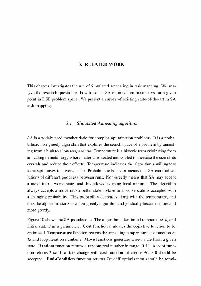
SA is a widely used metaheuristic for complex optimization problems. It is a proba-bilistic non-greedy algorithm that explores the search space of a problem by anneal-ing from a high to a low temperature. Temperature is a historic term originating fromannealing in metallurgy where material is heated and cooled to increase the size of itscrystals and reduce their effects. Temperature indicates the algorithm’s willingnessto accept moves to a worse state. Probabilistic behavior means that SA can find so-lutions of different goodness between runs. Non-greedy means that SA may accepta move into a worse state, and this allows escaping local minima. The algorithmalways accepts a move into a better state. Move to a worse state is accepted witha changing probability. This probability decreases along with the temperature, andthus the algorithm starts as a non-greedy algorithm and gradually becomes more andmore greedy.
Figure 10 shows the SA pseudocode. The algorithm takes initial temperature T0 andinitial state S as a parameters. Cost function evaluates the objective function to beoptimized. Temperature function returns the annealing temperature as a function ofT0 and loop iteration number i. Move functions generates a new state from a givenstate. Random function returns a random real number in range [0,1). Accept func-tion returns True iff a state change with cost function difference ∆C > 0 should beaccepted. End-Condition function returns True iff optimization should be termi-

20 3. Related work
nated. Parameters of the end conditions are not shown in the pseudocode. These mayinclude measures such as the number of consecutive rejected moves, current and agiven final temperature, current and accepted final cost. Finally the algorithm returnsthe best state Sbest in terms of the Cost function.
SIMULATED ANNEALING(S,T0)
1 C← COST(S)2 Sbest ← S3 Cbest ←C4 for i← 0 to ∞
5 do T ← TEMPERATURE(T0, i)6 Snew←MOVE(S,T )7 Cnew← COST(Snew)
8 ∆C←Cnew−C9 if ∆C < 0 or RANDOM()< ACCEPT(∆C,T )
10 then if Cnew <Cbest
11 then Sbest ← Snew
12 Cbest ←Cnew
13 S← Snew
14 C←Cnew
15 if END-CONDITION()16 then break17 return Sbest
Fig. 10. Pseudocode of the Simulated Annealing (SA) algorithm
3.2 SA in task mapping
Table 1 shows SA usage for 14 publications, each of which are summarized be-low. All publications apply SA for task mapping, five publications use SA for taskscheduling, and one for communication routing. None uses SA simultaneously forall purposes. There are many more publications that use different methods for taskmapping, but they are outside the scope of this Thesis. Synthetic task mapping meansthe paper uses task graphs that are not directed toward any particular application, butbenchmarking the mapping algorithms.

3.2. SA in task mapping 21
Table 1. Table of publications and problems where Simulated Annealing is applied. Taskmapping with SA is applied in a publication when “Mapping sel.” column is “Y”.Task scheduling and communication routing with SA is indicated similarly with“Sched. sel.” and “Comm. sel.” columns, respectively. All 14 publications applySA to task mapping in this survey, five to task scheduling, and one to communicationrouting.
Mapping Sched. Com. ApplicationPaper sel. sel. sel. field
Ali [2] Y N N QoS in multisensorshipboard computer
Bollinger [8] Y N Y Synthetic task mappingBraun [9] Y N N Batch processing tasksCoroyer [20] Y Y N Synthetic task mappingErcal [24] Y N N Synthetic task mappingFerrandi [25] Y Y N C applications partitioned with
OpenMP: Crypto, FFT, Imagedecompression, audio codec
Kim [43] Y Y N Synthetic task mappingKoch [45] Y Y N DSP algorithmsLin [56] Y N N Synthetic task mappingNanda [58] Y N N Synthetic task mappingOrsila [P7] Y N N Synthetic task mappingRavindran [61] Y Y N Network processing:
Routing, NAT, QoSWild [85] Y N N Synthetic task mappingXu [88] Y N N Artificial intelligence:
rule-based expert system
# of publications 14 5 1

22 3. Related work
Ali [2] optimizes performance by mapping continuously executing applications forheterogeneous PEs and interconnects while preserving two quality of service con-straints: maximum end-to-latency and minimum throughput. Mapping is optimizedstatically to increase QoS safety margin in a multisensor shipboard computer. Tasksare initially mapped by a fast greedy heuristics, after which SA further optimizesthe placement. SA is compared with 9 other heuristics. SA and GA were the bestheuristics in comparison. SA was slightly faster than GA, with 10% less runningtime.
Bollinger [8] optimizes performance by mapping a set of processes onto a multipro-cessor system and assigning interprocessor communication to multiple communica-tion links to avoid traffic conflicts. The purpose of the paper is to investigate taskmapping in general.
Braun [9] optimizes performance by mapping independent (non-communicating) gen-eral purpose computing tasks onto distributed heterogeneous PEs. The goal is to exe-cute a large set of tasks in a given time period. An example task given was analyzingdata from a space probe, and send instructions back to the probe before communica-tion black-out. SA is compared with 10 heuristics, including GA and TS. GA, SAand TS execution times were made approximately equal to compare effectiveness ofthese heuristics. GA mapped tasks were 20 to 50 percent faster compared to SA. Tabumapped tasks were 50 percent slower to 5 percent faster compared to SA. SA was runwith only one mapping per temperature level, but repeating the annealing process 8times for two different temperature coefficients. One mapping per temperature levelmeans insufficient number of mappings for good exploration. However, GA is betterwith the same number of mappings. GA gave the fastest solutions.
Coroyer [20] optimizes performance excluding communication costs by mapping andscheduling DAGs to homogeneous PEs. 7 SA heuristics are compared with 27 listscheduling heuristics. SA results were the best compared to other heuristics, but SA’srunning time was two to four orders of magnitude higher than other heuristics. Thepurpose of the paper is to investigate task mapping and scheduling in general.
Ercal [24] optimizes performance by mapping DAGs onto homogeneous PEs anda network of homogeneous communication links. Load balancing constraints aremaintained by adding a penalty term into the objective function. Performance isestimated with a statistical measure that depends on task mapping, communication

3.2. SA in task mapping 23
profile of tasks and the distance of communicating tasks on the interconnect network.Simulation is not used. The model assumes communication is Programmed IO (PIO)rather than DMA. SA is compared with a proposed heuristics called Task Allocationby Recursive Mincut. SA’s best result is better than the mean result in 4 out of 7 cases.Running time of SA is two orders of magnitude higher than the proposed heuristics.
Ferrandi [25] optimizes performance by mapping and scheduling a Hierarchical TaskGraph (HTG) [26] onto a reconfigurable MPSoC of heterogeneous PEs. HTGs weregenerated from C programs parallelized with OpenMP [70]. SA is compared withAnt Colony Optimization (ACO) [23], TS and a FIFO scheduling heuristics com-bined with first available PE mapping. SA running time was 28% larger than ACOand 12% less than TS. FIFO scheduling heuristics happens during run-time. SA gives11% worse results (performance of the solution) than ACO and comparable resultswith TS.
Kim [43] optimizes performance by mapping and scheduling independent tasks thatcan arrive at any time to heterogeneous PEs. Tasks have priorities and soft deadlines,both of which are used to define the performance metric for the system. Dynamicmapping is compared to static mapping where arrival times of tasks are known aheadin time. SA and GA were used as a static mapping heuristics. Several dynamicmapping heuristics were evaluated. Dynamic mapping run-time was not given, butthey were very probably many orders of magnitude lower than static methods becausedynamic methods are executed during the application run-time. Static heuristics gavenoticeably better results than dynamic methods. SA gave 12.5% better performancethan dynamic methods, and did slightly better than GA. SA run-time was only 4% ofthe GA run-time.
Koch [45] optimizes performance by mapping and scheduling DAGs presenting DSPalgorithms to homogeneous PEs. SA is benchmarked against list scheduling heuris-tics. SA is found superior against other heuristics, such as Dynamic Level Scheduling(DLS) [78]. SA does better when the proportion of communication time increasesover the computation time, and the number of PEs is low.
Lin [56] optimizes performance while satisfying real-time and memory constraintsby mapping general purpose synthetic tasks to heterogeneous PEs. SA reaches aglobal optimum with 12 node graphs.
Nanda [58] optimizes performance by mapping synthetic random DAGs to homoge-

24 3. Related work
neous PEs on hierarchical buses. The performance measure that is optimized is anestimate of expected communication costs and loss of parallelism with respect to crit-ical path (CP) on each PE. Schedule is obtained with list scheduling heuristics. TwoSA methods are presented where the second one is faster in run-time but gives worsesolutions. The two algorithms reach within 2.7% and 2.9% of the global optimumfor 11 node graphs.
Ravindran [61] optimizes performance by mapping and scheduling DAGs with re-source constraints on heterogeneous PEs. SA is compared with DLS and a decom-position based constraint programming approach (DA). DLS is the computationallymost efficient approach, but it loses to SA and DA in solution quality. DLS runs inless than a second, while DA takes up to 300 seconds and SA takes up to 5 seconds.DA is an exact method based on constraint programming that wins SA in solutionquality in most cases, but is found to be most viable for larger graphs where con-straint programming fails due to complexity of the problem space.
Wild [85] optimizes performance by mapping and scheduling DAGs to heterogeneousPEs. PEs are processors and accelerators. SA is compared with TS, FAST [49] [50]and a proposed Reference Constructive Algorithm (ReCA). TS gives 6 to 13 percent,FAST 4 to 7 percent, and ReCA 1 to 6 percent better application execution time thanSA. FAST is the fastest optimization algorithm. FAST is 3 times as fast than TS for100 node graphs and 7 PEs, and 35 times as fast than SA. TS is 10 as fast as SA.
Xu [88] optimizes performance of a rule-based expert system by mapping dependentproduction rules (tasks) onto homogeneous PEs. A global optimum is solved for theestimate by using linear programming (LP) [57]. SA is compared with the globaloptimum. SA reaches within 2% of the global optimum in 1% of the optimizationtime compared to LP. The cost function is a linear estimate of the real cost. In thissense the global optimum is not real.
3.3 SA parameters
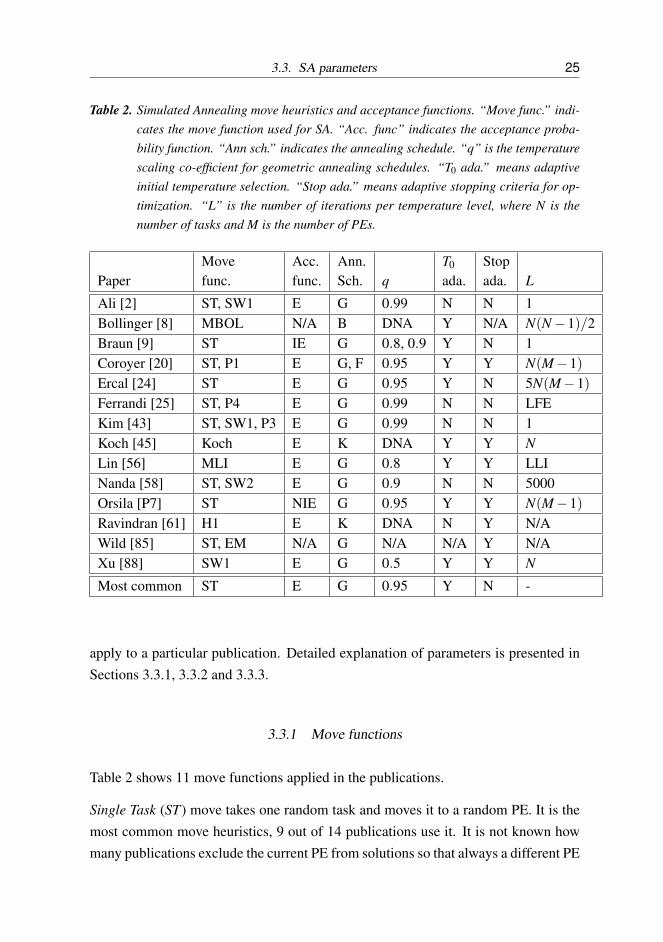
Table 2 shows parameter choices for the previous publications. Move and acceptancefunctions, and annealing schedule, and the number of iterations per temperature levelwas investigated, where N is the number of tasks and M is the number of PEs. “N/A”indicates the information is not available. “DNA” indicates that the value does not
3.3. SA parameters 25
Table 2. Simulated Annealing move heuristics and acceptance functions. “Move func.” indi-cates the move function used for SA. “Acc. func” indicates the acceptance proba-bility function. “Ann sch.” indicates the annealing schedule. “q” is the temperaturescaling co-efficient for geometric annealing schedules. “T0 ada.” means adaptiveinitial temperature selection. “Stop ada.” means adaptive stopping criteria for op-timization. “L” is the number of iterations per temperature level, where N is thenumber of tasks and M is the number of PEs.
Move Acc. Ann. T0 StopPaper func. func. Sch. q ada. ada. L
Ali [2] ST, SW1 E G 0.99 N N 1Bollinger [8] MBOL N/A B DNA Y N/A N(N−1)/2Braun [9] ST IE G 0.8, 0.9 Y N 1Coroyer [20] ST, P1 E G, F 0.95 Y Y N(M−1)Ercal [24] ST E G 0.95 Y N 5N(M−1)Ferrandi [25] ST, P4 E G 0.99 N N LFEKim [43] ST, SW1, P3 E G 0.99 N N 1Koch [45] Koch E K DNA Y Y NLin [56] MLI E G 0.8 Y Y LLINanda [58] ST, SW2 E G 0.9 N N 5000Orsila [P7] ST NIE G 0.95 Y Y N(M−1)Ravindran [61] H1 E K DNA N Y N/AWild [85] ST, EM N/A G N/A N/A Y N/AXu [88] SW1 E G 0.5 Y Y N
Most common ST E G 0.95 Y N -
apply to a particular publication. Detailed explanation of parameters is presented inSections 3.3.1, 3.3.2 and 3.3.3.
3.3.1 Move functions
Table 2 shows 11 move functions applied in the publications.
Single Task (ST) move takes one random task and moves it to a random PE. It is themost common move heuristics, 9 out of 14 publications use it. It is not known howmany publications exclude the current PE from solutions so that always a different PE

26 3. Related work
is selected by randomization. Excluding the current PE is useful because evaluatingthe same mapping again on consecutive iterations is counterproductive.
EM [85] is a variation of ST that limits task randomization to nodes that have aneffect on critical path length in a DAG. The move heuristics is evaluated with SAand TS. SA solutions are improved by 2 to 6 percent, TS solutions are not improved.Using EM multiplies the SA optimization time by 50 to 100 times, which indicates itis dubious by efficiency standards. However, using EM for TS approximately halvesthe optimization time!
Swap 1 (SW1) move is used in 3 publications. It chooses 2 random tasks and swapstheir PE assignments. These tasks should preferably be mapped on different PEs.MBOL is a variant of SW1 where task randomization is altered with respect to an-nealing temperature. At low temperatures tasks that are close in system architectureare considered for swapping. At high temperatures more distant tasks are considered.
Priority move 4 (P4) is a scheduling move that swaps the priorities of two randomtasks. This can be viewed as swapping positions of two random tasks in a task per-mutation list that defines the relative priorities of tasks. P1 is a variant of P4 thatconsiders only tasks that are located on the same PE. A random PE is selected at first,and then priorities of two random tasks on that PE are swapped. P3 scheduling moveselects a random task, and moves it to a random position in a task permutation list.
Hybrid 1 (H1) is a combination of both task assignment and scheduling simultane-ously. First ST move is applied, and then P3 is applied to the same task to set arandom position on a permutation list of the target PE. Koch [45] is a variant of H1that preserves precedence constraints of the moved task in selecting the random po-sition in the permutation of the target PE. That is, schedulable order is preserved inthe permutation list.
MLI is a combination of ST and SW1 that tries three mapping alterations. First, triesST greedily. The move heuristics terminates if the ST move improves the solution,otherwise the move is rejected. Then SW1 is tried with SA acceptance criterion. Themove heuristics terminates if the acceptance criterion is satisfied. Otherwise, ST istried again with SA acceptance criterion.
ST is the most favored mapping move. Heuristics based on swapping or movingpriorities in the task priority list are the most favored scheduling moves. The choiceof mapping and scheduling moves has not been studied thoroughly.
3.3. SA parameters 27
3.3.2 Acceptance functions
Table 2 shows acceptance functions for the publications. Acceptance function takesthe change in cost ∆C and temperature T as parameters. There are 3 relevant cases todecide whether to accept or reject a move. The first case ∆C < 0 is trivially accepted.The second case ∆C = 0 is probabilistically often accepted. The probability is usually0.5 or 1.0. The third case ∆C > 0 is accepted with a probability that decreases whenT decreases or ∆C grows.
Exponential acceptor function (E)
Accept(∆C,T ) = exp(−∆C
T). (1)
is the most common choice. Orsila [P7] uses the normalized inverse exponentialfunction (NIE)
Accept(∆C,T ) =1
1+ exp( ∆C0.5C0T )
. (2)
where T is in normalized range (0,1] and C0 is the initial cost. Inverse exponentialfunction is also known as the negative side of a logistic function f (x) = 1
1+exp(−x) .Braun [9] uses an inverse exponential function (IE)
Accept(∆C,T ) =1
1+ exp(∆CT )
. (3)
where T0 is set to C0. Temperature normalization is not used, but the same effect isachieved by setting the initial temperature properly.
Using an exponential acceptor with normalization and a proper initial temperatureis the most common choice. This choice is supported by the experiment in Sec-tion 6.2.1.
3.3.3 Annealing schedule
Table 2 shows annealing schedules for the publications. The annealing schedule isa trade-off between solution quality and optimization time. The annealing sched-ule defines the temperature levels and the number of iterations for each temperaturelevel. Optimization starts at the initial temperature T0 and ends at final temperatureTf . These may not be constants, in which case initial temperature selection and/orstopping criteria are adaptive. Stopping criteria defines when optimization ends.

28 3. Related work
Geometric temperature scale (G) is the most common annealing schedule. Temper-ature T is multiplied by a factor q ∈ (0,1) to get the temperature for the next level.That is, Tnext = qT . Usually several iterations are spent on a given temperature levelbefore switching to the next level. q is most often 0.95 or 0.99 in literature. Someworks use q = 0.9 that is also used by Kirkpatrick [44] that presented SA. They usedSA for partitioning circuits to two chips. This is analogous to mapping tasks ontotwo PEs.
Bollinger [8], denoted B, computes a ratio R of minimum cost to average cost ona temperature level, and then applies a geometric temperature multiplier Tnext =
min(R,qL)T , where qL is an experimentally chosen lower bound for the temperaturemultiplier. qL varied in range [0.9,0.98].
Ravindran [61] and Koch [45], denoted K, use a dynamic q factor that depends on thestatistical variance of cost at each temperature level. The temperature is calculatedwith
Tnext =T
1+ T ln(1+δ)3σT
(4)
where δ is an experimental parameter used to control the temperature step size andσT is the standard deviation of cost function on temperature level T . Higher δ orlower σT means a more rapid decrease in temperature. Koch suggests δ in range[0.25,0.50].
Coroyer [20] experimented with a fractional temperature scale (F). Temperature T iscalculated as Ti =
T0i where T0 is the initial temperature and i is the iteration number
starting from 1. Fractional temperature was found to be worse than geometric.
The normalized exponential acceptor
Accept(∆C,T ) = exp(−∆C
0.5C0T) (5)
and the normalized inverse exponential acceptor (2) put T0 to a range (0,1] whereinitial acceptance probabilities are adjusted to the initial cost.
The choice of initial temperature T0 can be chosen experimentally or methodically.[P2] [P6] [P7] [9] [8] [20] [24] [45] [56] [88] present methods to set T0 based ongiven problem space characteristics and desired acceptance criteria for moves. [P2][P6] [P7] determine T0 from the task graph and the system architecture. T0 can beset purely based on simulation so that T0 is raised high enough so that average move

3.3. SA parameters 29
acceptance probability p is high enough for aggressive statistical sampling of theproblem space [20] [45]. Often p∼ 0.9.
There are several common stopping criteria. Optimization ends when a given Tf hasbeen reached [20] [45], a given number of consecutive rejections happen, a givennumber of consecutive moves has not improved the solution, a given number ofconsecutive solutions are identical [20], or a solution (cost) with given quality isreached [45]. These criteria can also be combined. Constants associated with thesecriteria are often decided experimentally, but adaptive solutions exist too. [P2] [P6][P7] use a Tf that is computed from problem space.
The number of iterations per temperature level L is defined as an experimental con-stant or a function of the problem space. A function of the problem space is morewidely applicable, but a constant can be more finely tuned to a specific problem. L isoften dependent on N and M. Ercal [24] proposes L that is proportional to N(M−1),the number of neighboring solutions in the mapping space. Publications in this Thesisuse the same principle.
Lin [56] uses an adaptive number of iterations per temperature level (LLI). Theirapproach starts with L0 = N ∗ (N + M) for T0. The number of iterations for thenext temperature level is calculated by Lnext = min(1.1L,N(N + M)2). However,on each temperature level they compute an extra X −L iterations iff X > L, whereX = 1
exp((Cmin−Cmax)/T ) and Cmin and Cmax are the minimum and maximum costs onthe temperature level T . They compute initial temperature as T0 = a+ b, where ais the maximum execution cost of any task at any PE, and b is the maximum com-munication cost between any two tasks. Then they compute T0 average and standarddeviation of cost at T0 by sampling a number of moves. The temperature is doubled(once) if the minimum and maximum cost is not within two standard deviations fromthe average.
Ferrandi [25] has adaptive number of iterations per temperature level (LFE). Temper-ature level is switched on the first accepted on the temperature level. However, therecan be arbitrarily many rejected moves.

30 3. Related work

4. PUBLICATIONS
This chapter presents the problem space, research questions and contributions forPublications [P1-P7].
4.1 Problem space for Publications
Publications for this Thesis focus on mapping N tasks to M PEs, where tasks areinterdependent general purpose computational tasks which can be executed in a finitetime, i.e. the tasks are guaranteed to terminate within a specific time.
Applications in [P1-P6] are directed acyclic task graphs (DAGs), which are a specialcase of KPNs. The graphs were obtained from Standard Task Graph (STG) collec-tion [81]. Scheduling is done with the longest path heuristics, which defines taskpriority to be the longest path from a node to its exit nodes. The longest path is alsocalled the critical path. Nodes on the critical path are scheduled first. Applicationsare KPNs in [P7]. FIFO scheduling is used for KPN tasks. Tasks get scheduled inthe order they become ready. Cycle costs for operations and communication messagesizes are embedded directly into DAG and KPN models.
PEs are general purpose processors. PEs are homogeneous in [P1-P4, P6-P7], andheterogeneous in [P5]. PEs are connected with one or more communication links thateach have a given throughput, latency and arbitration latency.
Execution time is a part of the objective space in all publications. [P3] also consid-ers memory consumption due to communications buffering. [P5] considers energyconsumption with given silicon area constraints in the problem space.

32 4. Publications
Table 3. Scope of publications based on optimization criteria and research questionsP1 P2 P3 P4 P5 P6 P7
Optimized variablesExec. time × × × × × × ×
Memory ×Area/energy ×
Multi-objective ×Mapping algorithm
Convergence rate analysis × × × × ×Run time optimized × × × ×
Global optimum comparison ×Research questions analyzed
1. Parameter selection in a DSE point × × × × × ×2. Number of mappings and convergence ×
3. Parameters and convergence × × × × ×4. How to speedup convergence × × × ×
5. Converge rate ×
4.2 Research questions
The contribution of the Thesis is systematic analysis of the five research questionspresented in Section 1.3.
Table 3 shows the scope of publications based on optimization criteria and researchquestions.
First research question How to select optimization parameters for a given point inDSE problem space? Parameter selection should factor in complexity which is de-fined by a given design point in the problem space. E.g. more PEs or tasks shouldimply more iterations for the algorithm to explore a sufficient part of the implemen-tation space. It may also be that successful optimization is not a result of sufficientnumber of iterations, but entirely a different strategy is needed for different points inthe problem space. A single set of parameters should not be used for multiple pointsin the problem space that have different complexities. Optimization effort is thenwasted for simpler problems, but too little effort is used for more complex problems.

4.2. Research questions 33
To find results we analyzed the effect of parameter selection for varying problemcomplexity. The benefit of mapping iterations versus problem complexity is weighed.Reliability of the methods was tested with small graphs, and scalability with largergraphs.
Second research question How many mapping iterations are needed to reach a givensolution quality? The problem is NP-complete [59], and the difficulty of problemvaries with respect to application and HW complexity. The global optimum is usuallynot known, and therefore, is not known either how far a given solution is from theoptimum. This makes termination criteria for optimization hard to decide. A veryfast evaluation cycle is needed to find global optimum solutions for even a simpleand very constrained HW/SW system.
We examined the mapping iterations versus solution quality by obtaining global op-timum solutions for small graphs and simple HW systems by brute force search.
Third research question How does each parameter of the algorithm affect the con-vergence rate? Each parameter may have a different effect depending on the point inproblem space. Parameters can be compared with each other by altering them in thesame point in problem space.
To find results we analyzed optimization convergence rate based on the effect of ini-tial and final temperature, the number of mapping iterations per temperature level,different SA acceptance functions and the zero transition probability of the accep-tance function.
Fourth research question How to speedup convergence rate? That is, how to de-crease the run-time of mapping algorithm? Lot of the optimization can be ineffective.Effect of past optimization can be undone by later stages of optimization by changingthe same or related task mappings obtained before.
We found out a way to compute initial and final temperatures to speed up optimiza-tion. Also, Optimal Subset Mapping algorithm is presented that converges rapidly.
Fifth research question How often does the algorithm converge to a given solutionquality? Many combinatorial optimization algorithm, such as SA, rely on probabilis-

34 4. Publications
tic chance. Some estimates are needed how many times a probabilistic algorithmneeds to be run to obtain a solution of given quality.
To increase reliability of our results we applied the methods on both small and largegraphs. Small graphs and small number of PEs was exploited to obtain a globaloptimum comparison. Global optimum results give us an absolute reference on theconvergence rate of the algorithms. For example, a method may converge within 5%of the global optimum solution in 10% of the optimization runs.
4.3 Hybrid Algorithm for Mapping Static Task Graphs on MultiprocessorSoCs
[P1] proposes a Hybrid Algorithm (HA) to automatically distribute task graphs ontoa multiprocessor system to speedup execution. Research question 1 is analyzed. Themultiprocessor system had 2, 3 or 4 PEs connected with a shared bus, but no sharedmemory. Message passing was used to carry out computation in parallel.
The Hybrid Algorithm is a combination of three algorithms: Fast Pre-mapping (FP),GM and SA. FP is used initially to place tasks tasks rapidly on separate processors.FP automatically places children of a task graph node to separate PEs to rapidly startwith a parallel solution. This is not intended to be a good solution. The idea is toexploit trivial parallelism in the beginning of optimization to save mapping iterations.SA and GM are used after FP. SA and GM are used for global search, and GM is usedfor local search. The algorithm start with a full annealing temperature range, and iter-atively run SA by halving the initial temperature but keep the final temperature fixed.The SA would become finer grained on each iteration, because its initial temperaturewould be greedier on each iteration. GM is run after each SA iteration to optimizeeasy task placements with a greedy local search method. Iterating the process wouldrepeatedly find better and better solutions. The best solution seen during the processwould be returned.
HA is not efficient because the SA’s final temperature is set too low so that greedyoptimization has already happened before GM is used. Therefore, GM is not needed.GM could be useful if it were the case that SA stopped before it got greedy. That is,the final temperature of SA would have to be higher.
The only real practical approach in this algorithm was to use SA by running it itera-

Parameterizing Simulated Annealing for Distributing Task Graphs on multiprocessor 35
tively, and return the best result seen from all iterations. This could have been donewithout initial temperature adjustments, although halving the initial temperature ateach iteration could be a heuristics for determining how many times to run the SAbefore stopping. This algorithm was shown to be wasteful in terms of optimizationiterations in [P4].
It was later discovered that the experiment failed because there was insufficient num-ber of mapping iterations per SA optimization. There was too few iterations pertemperature level, and the final temperature was too high. SA would not converge ona good solution for these reasons. Also, there was a possibility of premature termina-tion before the final temperature. This showed us that manual parameter selection iserror-prone, and the failure motivated us to devise methods for automatic parameterselection. SA+AT was created for this reason.
4.4 Parameterizing Simulated Annealing for Distributing Task Graphs onmultiprocessor SoCs
[P2] proposes SA+AT method that automatically parameterizes SA. Research ques-tions 1, 3 and 4 are analyzed. The presented method decreases optimization timeand increases application speed. A trade-off is made between optimization time andoptimized execution time. The goal is to find a reliable optimization method that triesto search broad regions in the problem space, but also focus on the attractive parts ofthe space with more effort. This requires a careful annealing schedule, and possiblyseveral independent runs of the algorithm. The method saved 50% of optimizationtime in an experiment by only marginally slowing down the application.
The method takes the basic philosophy that the number of iterations and the tem-perature range is determined by the structure of the given application and hardwarearchitecture. The more complex the application or hardware the more iterations areneeded to converge to a good mapping reliably. Exponential time algorithms aredirectly rejected so that the method can be applied for large problems.
The method parameterizes SA by looking at the number of PEs and tasks, and taskexecution times on PEs. The method scales up with problem space complexity. Thenumber of mappings per temperature level is set with respect to the number of PEsand tasks. The number of temperature levels is based on task execution times on PEs.

36 Parameterizing Simulated Annealing for Distributing Task Graphs on multiprocessor
The PEs can be heterogeneous which affects the number of temperature levels.
The annealing schedule is defined by the number of iterations per temperature levelL, initial and final temperatures, and the coefficient q that defines a geometric tem-perature schedule.
Transition probability is defined so that transition probabilities occur within an effec-tive range, and the temperature range is normalized into (0,1]. The method needs avalue for the k variable, which determines a safety margin for initial and final tem-perature. Using k = 2 has been found sufficient, if not overly paranoid, in our papers.
A method is proposed to determined initial and final temperatures based on task ex-ecution times relative to application execution time on fastest and slowest processor.Initial temperature selection is not crucial in the sense that overestimation leads toexcessive optimization time, but does not make the final solution bad. The proposedmethod sets initial temperature high enough so that optimization effort is not wastedfor slowly converging chaotic random moves. Final temperature Tf selection is cru-cial, however. Too high Tf means greedy optimization opportunities are lost so thatpossible local minima are not found. Too low Tf means optimization time is wastedin a local minimum that does not converge anywhere else.
L is chosen to be N(M−1) and compared to different values with respect to applica-tion speedup. It is found that the given choice is appropriate for 300 task graphs with2 to 8 processors.
The method is tested with 10 random graphs (DAGs) with 50 nodes and 10 randomgraph with 300 nodes. The number of PEs is 2 to 8. The method is able to predict anefficient annealing schedule for the problem. The number of optimization iterationsis halved but optimized application’s execution time is increased only marginally.
4.5 Automated Memory-Aware Application Distribution forMulti-Processor System-On-Chips
[P3] proposes a method for optimizing memory consumption and execution timeof a task graph running on an MPSoC. Research questions 1 and 3 are analyzed.Parallelism is needed to speedup execution, but parallelism also increases memoryconsumption. The optimization algorithm uses an objective function that penalizesmemory consumption and execution time.

Optimal Subset Mapping And Convergence Evaluation of Mapping Algorithms 37
Memory consumption is optimized for three kinds of buffers: First, temporary resultsthat are stored on a PE waiting to be re-used on the same PE and then discarded.Second, temporary results that are stored on a PE waiting to be sent to another PEand then discarded. Third, input data from other PEs that is still being used by thePE.
SA, GM and RM algorithms are used to optimize two separate objective functions.The time-objective objective is used to optimize execution time. The memory-timeobjective is used to optimize both memory consumption and execution time.
The time-objective yields 2.12 speedup on average for SA, but also increases mem-ory consumption by 49%. The memory-time objective yields 1.63 speedup withoutincrease in memory consumption. The trade-off is 23% slower but 33% less memory.
The memory consumption trade-off is achieved by using the memory-time objectiveand adjusting the mapping by SA. Further memory savings would be possible byadjusting the schedule of the executed task graph to minimize the life-span of eachintermediate result. But it is beyond the scope of the paper.
4.6 Optimal Subset Mapping And Convergence Evaluation of MappingAlgorithms for Distributing Task Graphs on Multiprocessor SoC
[P4] proposes a fast mapping method called Optimal Subset Mapping (OSM). Re-search questions 1, 3 and 4 are analyzed. OSM is a divide and conquer [21] methodthat assumes that different parts of the problem can be optimized separately thatwould make the solution converge towards a global optimum. This assumption isnot valid for task mapping, but it can be a good strategy for other problems.
OSM takes a random subset of tasks and finds the optimum mapping in that subsetby trying all possible mappings (brute force search). This process is repeated bydecreasing and increasing the subset size within reasonable complexity limits. OSMis probabilistic because it chooses the subset randomly. It is also greedy because itonly accepts an improvement to the best known solution at each round.
OSM is compared with GM, HA, SA, SA+AT and RM. OSM was the most efficientalgorithm with respect to speedup divided by the number of iterations, but the abso-lute speedup was lower than with GM, HA, SA and SA+AT. OSM can be used as a

38 Evaluating of Heterogeneous Multiprocessor Architectures by Energy and Performance
starting point for a large optimization task because it converges rapidly. SA+AT isthe best algorithm overall. RM sets the baseline for all comparisons. Any algorithmshould do better than random mapping when systematic optimization opportunitiesexist in the problem space. GM, OSM, SA and SA+AT do much better than RM.
The algorithms were evaluated with a mapping that has 300 node random task graphsand 2, 4 and 8 PEs. OSM converges very rapidly initially. Convergence characteris-tics of OSM and GM are quite the opposite to each other, while the SA+AT method[P2] is in the middle. OSM loses against GM, SA and SA+AT in application speedup.On possible strategy to use OSM would be to start with OSM and switch to SA+ATwhen OSM does not increase the speedup anymore.
4.7 Evaluating of Heterogeneous Multiprocessor Architectures by Energyand Performance Optimization
[P5] analyzes a trade-off between energy consumption and performance among het-erogeneous MPSoCs. Pareto optimums are selected from a cloud of MPSoC candi-dates whose number of PEs and types of PEs varies with respect to performance, areaand power.
Task graphs were distributed onto a set of architecture, each architecture consistingof heterogeneous PEs. 141 architectures were tested with 10 graphs that each have300 nodes.
Energy consumption was estimated with static and dynamic energy parameters for3 cases: without dynamic energy (constant power), with little dynamic power, andwith more dynamic power. Well performing architectures were mostly the same inall cases. From low, medium and high speed PEs, the medium speed PEs were mostpower-efficient in the experiment.
Results from the experiment showed that SA method presented in [P2] shows goodconvergence properties for heterogeneous architectures too. The earlier paper usedhomogeneous PEs.
It was found that both energy-efficient and well performing solutions exist. However,most solutions were bad in all respects. The results indicate that good evaluation ofheterogeneous architectures requires good mapping when the mapping problem com-

4.8. Best Practices for Simulated Annealing in Multiprocessor Task Distribution Problems 39
plexity grows. Therefore, automated exploration tools are needed. SA+AT method ispresented and evaluated as a partial solution for this problem.
4.8 Best Practices for Simulated Annealing in Multiprocessor TaskDistribution Problems
[P6] is a survey of SA methods for task mapping. Research questions 1, 3 and 4are analyzed. SA parameterization is examined from existing publications. Commonannealing schedules, acceptance functions and termination conditions are presented.4 case studies are examined. Their relative properties, weaknesses and advantagesare compared.
The survey presents analytical insight into selection of initial and final temperaturesand the number of mappings L per temperature level. Optimization should be stoppedat final temperature Tf so that optimization effort is not wasted for greedy optimiza-tion that is stuck in a local optimum. SA+AT method presented in [P2] is analyzedmathematically. It is shown that SA+AT coefficient k is inverse exponentially propor-tional to the probability p f of accepting a worsening move on the final temperaturelevel.
The survey also presents 9 best practices for using SA with task mapping problems.It is argued that more attention should be put on reflecting problem space dimensionsin the SA parameters. A variety of SA parameters is recommended, including geo-metric temperature scaling coefficients, use of systematic methods for determinationof initial and final temperatures, and a suitable number of iterations per temperaturelevel. It is recommended that ST move heuristics should be used when in doubt,the same problem should be optimized multiple times to decrease the chance of badrandom chains, a normalized temperature range should be used.
The survey presents an idea that SA could be used as a main program for an applica-tion that continuously optimizes itself provided that the application tolerates variancein parameters and solutions. For example, run-time speed of the application could beoptimized on-the-fly to adapt to changing conditions. This discards real-time appli-cations, but can be adapted for throughput seeking applications.
Open research questions in SA task mapping are also presented. The question ofoptimal zero transition probability (∆C = 0) is answered in the Thesis.

40 Parameterizing Simulated Annealing for Distributing Kahn Process Networks
4.9 Parameterizing Simulated Annealing for Distributing Kahn ProcessNetworks on Multiprocessor SoCs
[P7] extends and improves the SA+AT method presented in [P2]. Research questions1 to 5 are analyzed. SA+AT is extended to support KPNs, which requires changesto parameter selection that determines an efficient annealing schedule. Optimizationtime is decreased with sensitivity analysis of tasks. Tasks with lowest executiontimes are ignored in the temperature range calculation to save optimization effort.Throwing the least time consuming set of processes, e.g. 5%, allows us to skip manytemperature levels for the final temperature, which saves optimization time. Qualityof results stayed approximately the same, but over half the optimization time wassaved. The method can be applied to general process networks, it is not limited toKPNs.
Convergence properties of the SA+AT method were analyzed by extensive simula-tions using graphs with varying difficulty. SA+AT convergence is compared to globaloptimum solutions that are found with a brute force search for 16 node graphs with 2and 3 PEs. Global optimum convergence rate varied from 0.2 percent to 35.8 percent.Numeric estimate is presented on the number of iterations to reach a global optimumby repeating SA+AT algorithm many times on the same problem. The number isbased on the global optimum convergence probability. We are not aware of a globaloptimum convergence experiments that are this extensive.
4.9.1 Corrected and extended results
Unfortunately, the simulation results were later found to be inaccurate due to a bugin the simulator code. The bug was that two tasks mapped on the same PE wouldtogether communicate over the shared interconnect instead of doing faster memoryoperations on the local memory bus that is exclusively dedicated to that PE. Thesimulator bug changed the optimization process so that the interconnect became anunnecessary bottleneck for all comunication. This was a performance bug, and thus,the applications ran much slower than they could. We fixed the communication bug,and we present the corrected results. Also, we extend the global optimum conver-gence results for 4 PEs.
The experiment was divided into setups A and B. We explain the effect of simulator

Parameterizing Simulated Annealing for Distributing Kahn Process Networks 41
bug in detail for setups A and B. The cost model for task communication is modelledas f (n)+g(n), where f (n) is the PE cost in time to handle communication layers forn bytes of data, and g(n) is the respective interconnect cost. For setup A, f (n) = 0.For setup B, f (n) is in O(n) for tasks communicating on different PEs and 0 for taskscommunicating on the same PE. Thus, the cost model in setup B favors that twocommunicating tasks are located on the same PE. The cost model in setup A doesnot favor placing communicating tasks on the same PE, because the f (n) is always0. The mapping process in setup A would merely place tasks so that schedule wouldmaximize interconnect utilization. Thus, the mapping process does not have the de-sired effect on performance. However, setup B convergence figures in the publicationare indicative of a properly working system because of the PE cost model that favorsplacing communicating tasks on the same PE.
The effectiveness of the automatic temperature method was evaluated again with afixed simulator. The test was the same as in the original publication, using 100 graphsfor each setup. The number of nodes varies from 16 to 256.
Table 4 shows speedups for setup A. This is the corrected version of Table III in[P7]. Table shows the minimum, mean, median and maximum speedups for SA+ATand SA+ST for 2 to 4 PEs. SA+ST is the same as SA+AT, but it doesn’t use thetemperature range computation method presented.
Table 5 shows the number of mappings for setup A. This is the corrected version ofTable IV in [P7]. SA+AT is less than 0.7 percent slower than SA+ST on average,but uses less than 38 percent of mapping iterations. The result tables for setup B areomitted; the numbers are similar. In short, SA+AT is at most 1.4 percent slower thanSA+ST on average, but uses less than 37 percent of mapping iterations.
Tables 6, 7, 8 and 9 are the corrected versions of Tables VII to X in [P7]. t is the op-timized application execution time, t0 is the global optimum. Table 6 and 7 show theconvergence rate to within p percent of global optimum for setups A and B, respec-tively. Results are also extended with 4 PE results. Table 8 and 7 show the expectedthe number of mappings it takes to repeat SA+AT to reach withing p percent of globaloptimum. Convergence results follow the same pattern with the fixed simulator as inthe original publication.
Global optimum was found in 0.3 to 38.3 percent of optimization runs with SA+AT.It was found that near global optimum are frequently obtained. Results within 1%

42 Parameterizing Simulated Annealing for Distributing Kahn Process Networks
Table 4. Automatic and static temperature compared: SA+AT vs SA+ST speedup values withsetup A. Higher value is better.
2 PEs 2 PEs 3 PEs 3 PEs 4 PEs 4 PEsSA+AT SA+ST SA+AT SA+ST SA+AT SA+ST
Min 1.781 1.817 2.296 2.347 2.612 2.585Mean 1.969 1.973 2.777 2.788 3.310 3.333Std 0.038 0.034 0.153 0.145 0.264 0.254Med 1.985 1.987 2.821 2.836 3.362 3.390Max 2.000 2.000 2.980 2.966 3.767 3.808
Table 5. Automatic and static temperature compared: SA+AT vs SA+ST number of mappingswith setup A. Lower value is better.
2 PEs 3 PEs 4 PEsSA+AT SA+ST SA+AT SA+ST SA+AT SA+ST
Min 473 2 900 1 190 5 800 2 170 8 690Mean 6 570 17 990 13 400 36 080 20 590 54 250Std 6 570 15 830 13 190 31 760 19 830 47 760Med 3 620 11 590 7 450 23 240 11 780 34 890Max 25 150 50 610 50 610 95 440 79 080 147 270

Parameterizing Simulated Annealing for Distributing Kahn Process Networks 43
Table 6. Brute force vs. SA+AT with setup A for 16 node graphs. Proportion of SA+AT runsthat converged within p from global optimum. Higher convergence proportion valueis better. Lower number of mappings is better.
Proportion of runs within limit p2 PEs 3 PEs 4 PEs
p = tto−1 acyclic cyclic acyclic cyclic acyclic cyclic
+0% 0.030 0.045 0.003 0.007 0.001 0.005+1% 0.323 0.124 0.006 0.019 0.004 0.012+2% 0.617 0.302 0.017 0.033 0.011 0.028+3% 0.819 0.529 0.040 0.061 0.021 0.050+4% 0.951 0.717 0.094 0.103 0.047 0.084+5% 0.990 0.853 0.177 0.158 0.089 0.135+6% 0.999 0.939 0.288 0.235 0.140 0.206+7% 1.000 0.977 0.447 0.330 0.210 0.285+8% 0.991 0.603 0.438 0.311 0.374+9% 0.999 0.745 0.555 0.427 0.459+10% 1.000 0.851 0.665 0.542 0.554+11% 0.927 0.753 0.665 0.641+12% 0.969 0.830 0.770 0.719+13% 0.988 0.890 0.862 0.791+14% 0.995 0.931 0.924 0.850+15% 0.999 0.960 0.963 0.897+16% 1.000 0.978 0.985 0.930+17% 0.990 0.994 0.956+18% 0.995 0.998 0.973+19% 0.998 0.999 0.985+20% 0.999 1.000 0.992+21% 1.000 0.996+22% 0.998+23% 1.000
mean mappings 765 800 1743 1754 2960 2943median mappings 770 761 1737 1721 2943 2956
are obtained in 0.6 to 46.0 percent of runs. Results within 2% are obtained in 1.7 to61.7 percent of runs. Results within 5% are obtained in 15.8 to 99.0 percent of runs.The results indicate that it is possible to save significant proportion of optimizationiterations by sacrificing a few percent of solution quality from the global optimum.

44 Parameterizing Simulated Annealing for Distributing Kahn Process Networks
Table 7. Brute force vs. SA+AT with setup B for 16 node graphs. Proportion of SA+AT runsthat converged within p from global optimum. Higher convergence proportion valueis better. Lower number of mappings is better.
Proportion of runs within limit p2 PEs 3 PEs 4 PEs
p = tto−1 acyclic cyclic acyclic cyclic acyclic cyclic
+0% 0.383 0.326 0.045 0.126 0.042 0.066+1% 0.460 0.388 0.088 0.160 0.067 0.076+2% 0.580 0.516 0.134 0.250 0.097 0.091+3% 0.647 0.560 0.188 0.323 0.140 0.116+4% 0.734 0.632 0.236 0.372 0.202 0.176+5% 0.783 0.661 0.337 0.422 0.267 0.210+6% 0.830 0.697 0.463 0.470 0.338 0.342+7% 0.883 0.712 0.564 0.497 0.427 0.395+8% 0.914 0.735 0.659 0.533 0.535 0.488+9% 0.931 0.748 0.747 0.595 0.620 0.536+10% 0.951 0.809 0.807 0.632 0.709 0.585+11% 0.960 0.853 0.858 0.665 0.781 0.627+12% 0.966 0.875 0.897 0.728 0.833 0.676+13% 0.972 0.901 0.925 0.761 0.874 0.721+14% 0.991 0.906 0.947 0.790 0.907 0.750+15% 0.994 0.911 0.969 0.820 0.932 0.777+16% 0.996 0.918 0.983 0.848 0.954 0.811+17% 0.996 0.923 0.990 0.868 0.968 0.837+18% 0.996 0.935 0.996 0.895 0.977 0.865+19% 0.997 0.941 0.998 0.915 0.984 0.877+20% 0.997 0.953 0.999 0.924 0.989 0.892+21% 0.998 0.959 1.000 0.943 0.995 0.900
. . . . . . . . . . . . . . . . . .+24% 1.000 0.965 0.972 0.999 0.924+25% 0.988 0.978 1.000 0.930+26% 0.994 0.981 0.935
. . . . . . . . . . . .+30% 1.000 0.993 0.966
. . . . . . . . .+37% 1.000 0.985
. . . . . .+48% 1.000
mean mappings 799 829 1649 1735 2661 2879median mappings 784 788 1627 1623 2647 2704

Parameterizing Simulated Annealing for Distributing Kahn Process Networks 45
Table 8. Brute force vs. SA+AT with setup A for 16 node graphs: Approximate number ofmappings to reach within p percent of global optimum. As a comparison to SA+AT,Brute force takes 32770 mappings for 2 PEs, 14.3M mappings for 3 PEs and 1.1Gmappings for 4 PEs. Lower value is better.
Number of mappings2 PEs 3 PEs 4 PEs
acyclic cyclic acyclic cyclic acyclic cyclicp SA+AT SA+AT SA+AT SA+AT SA+AT SA+AT
+0% 25 070 17 670 581 030 261 760 2 466 800 639 890+1% 2 370 6 470 290 520 89 940 740 040 247 350+2% 1 240 2 650 100 760 52 990 276 650 106 650+3% 930 1 510 44 130 28 700 143 700 58 990+4% 800 1 120 18 580 16 980 62 850 35 040+5% 770 940 9 840 11 080 33 300 21 850+6% ≤ 770 850 6 060 7 460 21 130 14 260+7% . . . 820 3 900 5 310 14 100 10 320+8% 810 2 890 4 000 9 510 7 870+9% 800 2 340 3 160 6 940 6 410
+10% ≤ 800 2 050 2 640 5 470 5 320+11% . . . 1 880 2 330 4 450 4 590+12% 1 800 2 110 3 840 4 100+13% 1 770 1 970 3 430 3 720+14% 1 750 1 880 3 200 3 470+15% 1 750 1 830 3 070 3 280+16% 1 740 1 790 3 010 3 160+17% . . . 1 770 2 980 3 080+18% 1 760 2 970 3 030+19% 1 760 2 960 2 990+20% 1 760 . . . 2 970+21% 1 750 2 960
. . . . . . . . .+25% 2 950

46 Parameterizing Simulated Annealing for Distributing Kahn Process Networks
Table 9. Brute force vs. SA+AT with setup B for 16 node graphs: Approximate number ofmappings to reach within p percent of global optimum. As a comparison to SA+AT,Brute force takes 32770 mappings for 2 PEs, 14.3M mappings for 3 PEs and 1.1Gmappings for 4 PEs. Lower value is better.
Number of mappings2 PEs 3 PEs 4 PEs
acyclic cyclic acyclic cyclic acyclic cyclicp SA+AT SA+AT SA+AT SA+AT SA+AT SA+AT
+0% 2 090 2 540 33 930 13 790 62 910 43 620+1% 1 740 2 140 18 630 10 840 39 600 37 730+2% 1 380 1 610 12 290 6 950 27 580 31 570+3% 1 240 1 480 8 750 5 370 19 060 24 860+4% 1 090 1 310 6 990 4 660 13 190 16 350+5% 1 020 1 250 4 900 4 110 9 990 13 740+6% 960 1 190 3 570 3 690 7 890 8 820+7% 910 1 160 2 920 3 490 6 240 7 290+8% 880 1 130 2 500 3 250 4 970 5 900+9% 860 1 110 2 210 2 920 4 290 5 370
+10% 840 1 030 2 040 2 740 3 750 4 930+11% 830 970 1 920 2 610 3 410 4 590+12% 830 950 1 840 2 380 3 190 4 260+13% 820 920 1 780 2 280 3 040 3 990+14% 810 920 1 740 2 200 2 940 3 840+15% 800 910 1 700 2 120 2 850 3 710+16% ≤ 800 900 1 680 2 050 2 790 3 550+17% . . . 900 1 670 2 000 2 750 3 440+18% 890 1 660 1 940 2 720 3 330+19% 880 1 650 1 900 2 700 3 280+20% 870 ≤ 1 650 1 880 2 690 3 230+21% 870 . . . 1 840 2 680 3 200+22% 860 1 830 2 670 3 160+23% 860 1 800 2 670 3 130+24% 860 1 780 2 660 3 120+25% 840 1 780 . . . . . .+26% 830 1 770 3 080+27% . . . 1 760 3 040
. . . . . . . . .+37% 1 740 2 920
. . . . . .+45% 2 880

5. DCS TASK MAPPER
5.1 DCS task mapper
DCS task mapper is a tool that does task mapping (placement) and scheduling forMPSoCs. Applications are modeled as DAGs or KPNs. Tasks are processes thatexecute on a PE, such as a processor or a HW accelerator. The tool tries to place eachtask to a PE so that a given objective function is minimized. The program supportsSA, GA, RM, GM, OSM, brute force and FP mapping algorithms.
The program is available at DACI research group web site [22] under an Open Sourcelicense: LGPL 2.1 [55]. The program was written in C with performance in mind tocarry out experiments for Publications [P2-P7]. [P1] used a Python prototype of theDCS task mapper. The tool, including the Python prototype, was written from scratchby the Author of the Thesis.
The program simulates a virtual system based on PEs and communication channels.Figure 11 shows the data flow and state transitions of the tool on a high level. Events,operations of tasks and communication messages are scheduled onto PEs and com-munication channels. Tasks compete for computation and communication time, butonly one task at a time may execute on a PE or communicate on a communicationchannel. The program reads a mapping-scheduling problem as input. The inputconsists of a virtual system architecture, task graph, optimization algorithm and itsparameters. The program maps task graph onto the system and schedules it to obtainobjective space values, e.g. execution time, power and area. Execution time, powerand area are annotated into architecture and task graph description. Time-level behav-ior is simulated according to annotated values. The system does not produce actualdata.
Time behavior and resource contention is simulated for PEs and communicationchannels onto which task computation and communication is mapped. The simulator

48 5. DCS task mapper
Input data
Parse input
problem
Optimization
heurististics
Cost function
evaluation
Evaluate a point
in problem space
Generate result
report
Terminate
Initialize
simulator tasks,
PEs and communication
Simulator
event loop
Schedule complete
PE ready
to execute
A ready task is
selected for execution
Communication ready
to transfer
A pending transfer
is selected
PE finished
computing job
Task blocks
Communication finished
transfering
Transfer
finished
Task blocksTask unblocked Unblock tasks
Issue pending
transfers
Task unblocked
Issue pending
transfers
Results
Fig. 11. DCS task mapper data flow and state transitions. Solid line indicates data flow.Dashed line indicates causality between events in the state machine.

5.2. Job clustering with jobqueue 49
event loop handles four events: transfer finished, computation finished, communica-tion channel ready to transfer and PE ready to compute.
Tasks consist of 3 kinds of operations: compute X cycles, read Y or write Z bytes ofdata onto a communication channel. This simple operation set makes fast schedulingand simulation possible. PE executes operations from a task until a blocking readoperation takes place, then a task switch takes place on the PE. When a task receivesdata that it needs to continue execution, it is unblocked. Tasks are waken up basedon task priorities. Task priorities are supported for scheduling optimization. DAGsuse critical path scheduling to set task priorities. KPNs use FIFO scheduling, butpriority based scheduling is supported too. An efficient heap data structure is used todetermine the task that has the most highest priority.
Communication scheduling can be optimized with different scheduling policies. FIFO,LIFO, priority and random order policies are supported. Critical path scheduling isused with DAGs. FIFO scheduling is used with KPNs. Adding new scheduling poli-cies is modular.
The program contains approximately 8200 lines of C [62] written for GNU/Linuxand UNIX-like systems. The program only depends on C library and a few systemcalls. The program was originally prototyped with a Python [63] implementation thatwas two orders of magnitude slower than the C implementation. Python was foundto be an excellent prototyping language for algorithms and simulation, but it was tooslow. Months of simulation time was reduced to days with a C implementation. TheC implementation took several computation months to complete the experiments ofthe publications.
The execution time of the task mapper is effectively dependent on the simulation part,and thus, the number of mappings tried by the optimization heuristics. Optimizationheuristics used consume less than one percent of the execution time. Table 10 showsthe number of mappings explored, the mapping speed and the time computed withDCS task mapper for publications [P2] [P3] [P4] [P5] [P7].
5.2 Job clustering with jobqueue
Publications [P1]-[P4] use shell scripts to distribute task mapping jobs into a clusterof 10 Gentoo Linux machines with 2.8GHz Pentium 4 processor. A shell script would
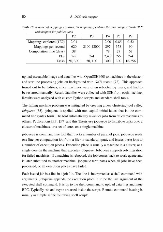
50 5. DCS task mapper
Table 10. Number of mappings explored, the mapping speed and the time computed with DCStask mapper for publications
P2 P3 P4 P5 P7
Mappings explored (1E9) 2.03 2.00 0.85 0.52Mappings per second 620 2100-12000 297 358 90
Computation time (days) 38 78 27 67PEs 2-8 2-4 2,4,8 2-5 2-4
Tasks 50, 300 50, 100 300 300 16-256
upload executable image and data files with OpenSSH [60] to machines in the cluster,and start the processing jobs on background with GNU screen [72]. This approachturned out to be tedious, since machines were often rebooted by users, and had tobe restarted manually. Result data files were collected with SSH from each machine.Results were analyzed with custom Python scripts and standard shell tools.
The failing machine problem was mitigated by creating a new clustering tool calledjobqueue [35]. jobqueue is spelled with non-capital initial letter, that is, the com-mand line syntax form. The tool automatically re-issues jobs from failed machines toothers. Publications [P5], [P7] and this Thesis use jobqueue to distribute tasks onto acluster of machines, or a set of cores on a single machine.
jobqueue is command line tool that tracks a number of parallel jobs. jobqueue readsone line per computation job from a file (or standard input), and issues these jobs toa number of execution places. Execution place is usually a machine in a cluster, or asingle core on the machine that executes jobqueue. Jobqueue supports job migrationfor failed machines. If a machine is rebooted, the job comes back to work queue andis later submitted to another machine. jobqueue terminates when all jobs have beenprocessed, or all execution places have failed.
Each issued job is a line in a job file. The line is interpreted as a shell command witharguments. jobqueue appends the execution place id to be the last argument of theexecuted shell command. It is up to the shell command to upload data files and issueRPC. Typically ssh and rsync are used inside the script. Remote command issuing isusually as simple as the following shell script:

5.2. Job clustering with jobqueue 51
#!/bin/sh
input="$1"
results="$2"
host="$3"
cat "$input" |ssh "$host" "nice -n 19 bin/taskmapper" \
> "$results"
bin/taskmapper is the DCS task mapper executable on the remote machine. Theinput is read from a data file that is piped through OpenSSH to the remote taskmapper.The remote taskmapper writes results to its standard output which is piped throughOpenSSH to a local result file. Minimal engineering and resources are needed tosetup this kind of system. No commercial software is needed.
Jobqueue has 2280 lines of C code, out of which 970 lines are dead code underprototype development. It was written by the Author of this Thesis. The source codeis available under Public Domain at [35].

52 5. DCS task mapper

6. SIMULATED ANNEALING CONVERGENCE
6.1 On global optimum results
This section analyzes research questions 2, 3 and 5. How many mapping iterationsare needed to reach a given solution quality? SA convergence rate and the number ofmapping iterations is compared with respect to global optimum solutions. How doeseach parameter of the algorithm affect the convergence rate and quality of solutions?The effect of L value and acceptance function is analyzed with respect to the numberof mapping iterations and solution quality. How often does the algorithm convergeto a given solution quality? We present convergence results with reference to globaloptimum solutions.
A global optimum is hard to find for large task graphs since the mapping problemis in NP-complexity class. Effectiveness of heuristics may decrease rapidly as thenumber of nodes grows. The total number of mappings X for N nodes and M PEs isX = NM. The number of mappings grows exponentially with respect to nodes, andpolynomially with respect to PEs. Adding PEs is preferable to adding nodes fromthis perspective.
[P7] analyzed global optimum convergence for 2 and 3 PE architectures and 16 nodeKPNs by using a brute force algorithm. The experiment is extended to 32 nodegraphs on 2 PEs. More than 2 PEs would be too costly to compute in brute forcefor 32 or more nodes. PE mapping was fixed for one node, which yields X = 231 ∼2.1× 10⁹ mappings for each graph. Fixing one node is a valid choice because PEsare homogeneous. The technical details of the experiment are explained in [P7].
Ten task graphs were generated with setup B in [P7]. Graphs were generated withkpn-generator [46] with following parameters: target distribution parameter 10%,cyclic graphs (default) and b-model parameter for both communication size and com-putation time as 0.7 (default). Target distribution defines the relative number of tasks

54 6. Simulated Annealing convergence
that can act as a target for each task. For example, 10% target distribution for a 32node graph means each task can communicate with at most 3 other tasks.
Global optimum results were compared to SA+AT by running SA+AT 1000 timesindependently for each graph. The proportion of SA+AT that come within p percentof global optimum was calculated. Table 11 shows the proportion of SA+AT runs thatgot execution time t ≤ (1+ p)to, where p is the execution time overhead comparedto global optimum execution time to. p = 0% means the global optimum (executiontime). p = 10% means execution time no more than 10% over the global optimum.The last two rows show mean and median values for the number of mappings tried ina single SA+AT run. Figure 12 shows the same values. SA uses 0.4 to 9 millionthsof the brute force iterations, but does not always converge to a global optimum.
Table 12 shows the expected number of mappings needed to obtain a result withinp percent of global optimum by repeatedly running SA+AT. The same values areplotted in Figure 13. These values are based on the mean iterations and probabilitiesin Table 11. Note, convergence is probabilistic, which means the actual global opti-mum might never be reached. SA uses on average 43 to 64 millionths of the bruteforce iterations to reach global optimum. Optimization time is reduced by 5 ordersof magnitude.
Brute force uses 2.0×10⁴ times the iterations compared to SA with L= 32, the choiceof SA+AT, and 2.3×10⁴ times iterations compared to SA with L = 64. Both valuesshow 4 orders of improvement over brute force. Results within 3% of global opti-mum are reached with 5 orders of magnitude improvement in iterations by using theSA+AT. Results within 16% are reached with 6 orders of magnitude improvement.
Figure 14 shows the task graph execution time for one graph plotted against the num-ber of mappings. All possible mapping combinations for 32 nodes and 2 PEs werecomputed with brute force search. One node mapping was fixed. 31 node mappingswere varied resulting into 231 = 2147483648 mappings. The initial execution time is875 µs, mean 1033 µs and standard deviation 113 µs. Table 13 shows the proportionof SA runs that converged within p percent of global optimum and the associatednumber of mappings within that range computed from the brute force search. Thereis only one mapping that is the global optimum: 535 µs. SA reaches the global opti-mum in 2.1% of the runs. Repeating SA yields the global optimum in approximately1E5 iterations. RM would find global optimum in 1E9 iterations in approximately

6.1. On global optimum results 55
Table 11. SA+AT convergence with respect to global optimum with L = 16,32,64,128 and256 for 32 nodes. Automatic parameter selection method in SA+AT chooses L =
32. Values in table show proportion of SA+AT runs that converged within p fromglobal optimum. Higher value is better.
Proportion of runs within limit pL value
p = tto−1 16 32 64 128 256
+0% 0.006 0.016 0.038 0.080 0.152+1% 0.010 0.026 0.061 0.129 0.232+2% 0.023 0.051 0.117 0.224 0.365+3% 0.039 0.084 0.173 0.311 0.477+4% 0.057 0.119 0.230 0.391 0.558+5% 0.076 0.154 0.287 0.468 0.649+6% 0.101 0.201 0.355 0.553 0.732+7% 0.137 0.264 0.439 0.653 0.834+8% 0.178 0.337 0.536 0.757 0.919+9% 0.220 0.400 0.606 0.819 0.949+10% 0.267 0.461 0.675 0.870 0.969+11% 0.319 0.531 0.747 0.917 0.985+12% 0.378 0.605 0.812 0.952 0.994+13% 0.449 0.664 0.864 0.972 0.998+14% 0.509 0.726 0.906 0.983 0.999+15% 0.568 0.780 0.935 0.992 1.000+16% 0.627 0.831 0.958 0.996+17% 0.681 0.868 0.974 0.998+18% 0.731 0.903 0.984 0.999+19% 0.778 0.930 0.990 0.999+20% 0.820 0.953 0.994 1.000+21% 0.853 0.968 0.997+22% 0.884 0.979 0.998+23% 0.908 0.985 0.999+24% 0.931 0.991 1.000+25% 0.947 0.995+26% 0.961 0.996+27% 0.971 0.998+28% 0.980 0.999+29% 0.987 1.000+30% 0.992
. . . . . .+37% 1.000
mean mappings 840 1 704 3 516 7 588 19 353median mappings 836 1 683 3 437 7 428 18 217

56 6. Simulated Annealing convergence
Table 12. Approximate expected number of mappings for SA+AT to obtain global optimumwithin p percent for L = 16,32,64,128 and 256 for 32 nodes. SA+AT choosesL = 32. Best values are in boldface on each row. Lower value is better.
Estimated number of mappingsL value
p 16 32 64 128 256
+0% 137741 108507 92766 94966 127744+1% 84022 65021 57921 58865 83347+2% 36531 33208 29947 33919 53023+3% 21767 20402 20334 24429 40556+4% 14793 14340 15300 19406 34683+5% 11099 11084 12242 16206 29820+6% 8311 8471 9907 13721 26439+7% 6155 6458 8001 11627 23208+8% 4723 5060 6561 10027 21059+9% 3812 4255 5804 9264 20402
+10% 3150 3695 5212 8724 19970+11% 2635 3208 4708 8276 19654+12% 2221 2817 4328 7972 19472+13% 1873 2564 4069 7810 19394+14% 1651 2348 3881 7717 19367+15% 1480 2183 3761 7647 19357+16% 1340 2051 3670 7618+17% 1234 1963 3609 7604+18% 1149 1886 3572 7595+19% 1080 1832 3550 7593+20% 1025 1787 3537 7589+21% 985 1760 3526+22% 950 1741 3524+23% 926 1730 3520+24% 903 1719 3518+25% 888 1713+26% 874 1710+27% 865 1706+28% 857 1705+29% 851 1704+30% 847+31% 845
. . . . . .+37% 841

6.1. On global optimum results 57
0 2 4 6 8 10 12 14 16 18 20 22 24 26 28 30 32 34 36 38 40
Percentage p over global optimum
0.001
0.01
0.1
1SA
converg
ence
pro
babili
ty
L = 16 L = 32 L = 64 L = 128 L = 256
Fig. 12. SA+AT convergence with respect to global optimum with L = 16,32,64,128 and 256for 32 nodes. SA+AT chooses L = 32. Lines show proportion of SA+AT runs thatconverged within p from global optimum for a given value of L. Lower p value onX-axis is better. Higher probability on Y-axis is better.
half the runs. RM only converges within 13% of the global optimum in a million iter-ations. Also, there is only one mapping that is the worst solution: 1708 µs. Reversingthe cost difference comparison in SA yields the worst solution in 0.9% of the runs.The SA algorithm can therefore also find the global maximum.
Table 14 shows global optimum convergence rate variance between graphs for L val-ues. Doubling L approximately doubles the mean convergence rate. Minimum andmaximum convergence rates vary by a factor of 50, approximately.
With L = 256 the hardest graph converged with probability 0.4%, but the same graphconverged within 1% with 4.4% probability, within 2% with 8.8% probability, andwithin 3% with 22.3% probability. Sacrificing just 3% from optimum more thandoubles the convergence rate on average, as shown by Table 11. The easiest graphconverged to optimum with 27.8% probability, but within 3% with just 32.6% prob-
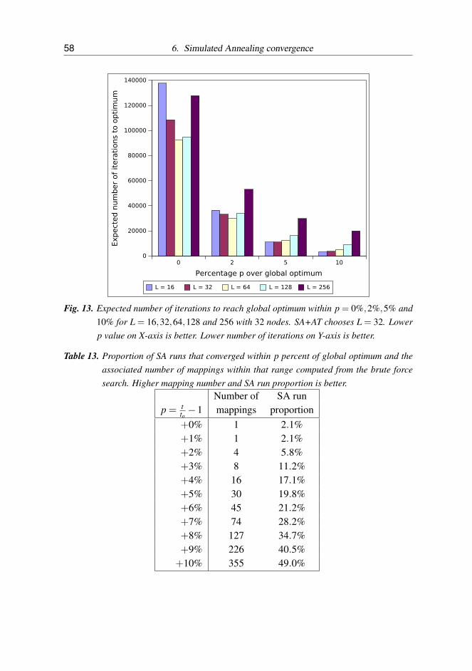
58 6. Simulated Annealing convergence
0 2 5 10
Percentage p over global optimum
0
20000
40000
60000
80000
100000
120000
140000
Exp
ect
ed
num
ber
of
itera
tions
to o
pti
mu
m
L = 16 L = 32 L = 64 L = 128 L = 256
Fig. 13. Expected number of iterations to reach global optimum within p = 0%,2%,5% and10% for L = 16,32,64,128 and 256 with 32 nodes. SA+AT chooses L = 32. Lowerp value on X-axis is better. Lower number of iterations on Y-axis is better.
Table 13. Proportion of SA runs that converged within p percent of global optimum and theassociated number of mappings within that range computed from the brute forcesearch. Higher mapping number and SA run proportion is better.
Number of SA runp = t
to−1 mappings proportion
+0% 1 2.1%+1% 1 2.1%+2% 4 5.8%+3% 8 11.2%+4% 16 17.1%+5% 30 19.8%+6% 45 21.2%+7% 74 28.2%+8% 127 34.7%+9% 226 40.5%
+10% 355 49.0%

6.1. On global optimum results 59
0 200 400 600 800 1000 1200 1400 1600 1800
Task graph execution time / us
1
10
100
1000
10000
100000
1000000
10000000
Num
ber
of
mappin
gs
/ 1
Task graph execution time vs number of mappings
Fig. 14. Task graph execution time for one graph plotted against the number of mappings. Allpossible mapping combinations for 32 nodes and 2 PEs were computed with bruteforce search. One node mapping was fixed. 31 node mappings were varied resultinginto 231 = 2147483648 mappings. The initial execution time is 875 µs, mean 1033µs and standard deviation 113 µs. There is only one mapping that reaches the globaloptimum 535 µs.
ability. This indicates there are not many solutions near the global optimum, buthitting the global optimum is rather probable (27.8%). This is opposite to the hard-est graph where hitting the global optimum is hard (probability 0.4%), but there aremany solutions within 3% that hit at 22.3% probability.
Experiment data, scripts and instructions how to repeat and verify the experiment areavailable at DCS task mapper web page [22] under the section “Experimental data”.A reference C implementation of the SA+AT algorithm is also available at [64]. Theexperiment can be repeated with a GNU/Linux system by using DCS task mapperand jobqueue [35]. Experiment scripts probe for available processors and use multi-processing to produce the results.

60 6. Simulated Annealing convergence
Table 14. Global optimum convergence rate varies between graphs and L values. The sampleis 10 graphs. Columns show the minimum, mean, median and maximum probabilityof convergence to global optimum, respectively. Value 0% in Min column meansthere was a graph for which global optimum was not found in 1000 SA+AT runs.For L≥ 32 global optimum was found for each graph. Note, the Mean column hassame values as the p = 0% row in Table 11.
L Min (%) Mean (%) Median (%) Max (%)
16 0.0 0.6 0.4 1.632 0.1 1.6 0.9 4.764 0.3 3.8 2.9 8.6128 0.3 8.0 6.9 15.7256 0.4 15.2 15.6 27.8
6.2 On SA acceptance probability
6.2.1 On acceptor functions
We analyze research question 3 in this section: How normalized exponential and in-verse exponential acceptor functions compare in solution quality and convergence?We ran an experiment to compare the normalized inverse exponential (2) and normal-ized exponential (5) acceptor functions. Parameter selection method from [P7] wasapplied to (5). The experiment was re-run for both acceptor functions, 100 graphs,2-4 PEs, 10 times each case, totaling 6000 optimization runs.
Table 15 shows gain results for both acceptor functions. Table 16 shows the numberof iterations. Exponential acceptor is not more than half a percent better in terms ofgain.
However, exponential acceptor loses up to 7% in the number of iterations. Both SAalgorithms have an equal number of iterations per temperature from T0 to Tf . Opti-mization terminates when T ≤ Tf and L consecutive rejections happen. Acceptancefunction affects the number of consecutive rejections which makes the difference inthe number of iterations. Inverse exponential acceptor has higher rejection probabil-ity, which makes it stop earlier than an exponential acceptor.
Very few papers try different acceptor functions. [P1-7] use inverse exponential func-tion. In retrospect it seems that exponential function would not have affected results

6.2. On SA acceptance probability 61
Table 15. Comparing average and median gain values for the inverse exponential and expo-nential acceptors. A is the mean gain for experiments run with inverse exponentialacceptor. B is the same for exponential acceptor. C and D are median gain valuesfor inverse exponential acceptor and exponential acceptor, respectively. Highervalue is better in columns A, B, C and D.
Mean gain Median gainPEs A B A
B −1 C D CD −1
2 1.329 1.334 −0.3% 1.314 1.316 −0.2%3 1.566 1.576 −0.6% 1.531 1.538 −0.5%4 1.794 1.798 −0.2% 1.757 1.761 −0.2%
Table 16. Comparing average and median iterations for the inverse exponential and expo-nential acceptors. E is the mean iterations for experiments run with inverse expo-nential acceptor. F is the same for exponential acceptor. G and H are the medianiterations for inverse exponential and exponential acceptors, respectively. Lowervalue is better in columns E, F, G and H.
Mean iterations Median iterationsPEs E F E
F −1 G H GH −1
2 6758 6882 −1.8% 4228 4272 −1.0%3 13577 14120 −3.8% 8456 8536 −1.0%4 20734 22398 −7.4% 12850 13806 −6.9%
significantly. It is possible that a better acceptor function exists, but these two areused most widely.
Furthermore, we compared brute force results with 32 nodes and 2 PEs between nor-malized exponential and normalized inverse exponential acceptors. Table 17 showsthe difference between global optimum converge rates for the two acceptors forSA+AT. Results indicate normalized exponential acceptor converges slightly morefrequently than normalized inverse exponential acceptor. The SA+AT choice L = 32displays difference of at most 2.4% in absolute convergence rate.
We recommend using normalized exponential acceptor for task mapping.
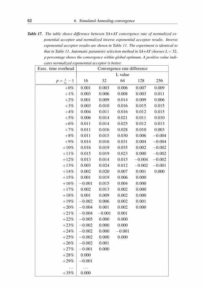
62 6. Simulated Annealing convergence
Table 17. The table shows difference between SA+AT convergence rate of normalized ex-ponential acceptor and normalized inverse exponential acceptor results. Inverseexponential acceptor results are shown in Table 11. The experiment is identical tothat in Table 11. Automatic parameter selection method in SA+AT chooses L = 32.p percentage shows the convergence within global optimum. A positive value indi-cates normalized exponential acceptor is better.
Exec. time overhead Convergence rate differenceL value
p = tto−1 16 32 64 128 256
+0% 0.001 0.003 0.006 0.007 0.009+1% 0.003 0.006 0.008 0.003 0.011+2% 0.001 0.009 0.014 0.009 0.006+3% 0.003 0.010 0.016 0.015 0.015+4% 0.004 0.011 0.016 0.012 0.015+5% 0.006 0.014 0.021 0.011 0.010+6% 0.011 0.014 0.025 0.012 0.013+7% 0.011 0.016 0.028 0.010 0.003+8% 0.011 0.015 0.030 0.006 −0.004+9% 0.014 0.016 0.031 0.004 −0.004
+10% 0.016 0.019 0.035 0.002 −0.002+11% 0.015 0.019 0.023 0.000 −0.002+12% 0.013 0.014 0.015 −0.004 −0.002+13% 0.003 0.024 0.012 −0.002 −0.001+14% 0.002 0.020 0.007 0.001 0.000+15% 0.001 0.019 0.006 0.000+16% −0.001 0.015 0.004 0.000+17% 0.002 0.013 0.002 0.000+18% 0.001 0.009 0.002 0.000+19% −0.002 0.006 0.002 0.001+20% −0.004 0.001 0.002 0.000+21% −0.004 −0.001 0.001+22% −0.005 0.000 0.000+23% −0.002 0.000 0.000+24% −0.002 0.000 −0.001+25% −0.002 0.000 0.000+26% −0.002 0.001+27% −0.001 0.000+28% 0.000+29% −0.001
. . . . . .+35% 0.000

6.3. On Comparing SA+AT to GA 63
6.2.2 On zero transition probability
SA acceptance function defines the probability to accept a move for a given objectivechange and the temperature. Zero transition probability is the probability of accept-ing a move that does not change the cost. We studied the effect of zero transitionprobability to the solution quality. This belongs to the category of the third researchquestion.
The normalized inverse exponential acceptance function (2) gives 0.5 probability forzero transition, that is, when ∆C = 0. The acceptance function was modified (6) totest the effect of zero transition probability:
Accept(∆C,T ) =2a
1+ exp( ∆C0.5C0T )
, (6)
a is the probability for ∆C = 0. SA+AT was re-run for several graphs with the setupspecific in detail in [P7] with distinct probabilities a∈ [0.1,0.2, . . . ,1.0]. Two 16 nodecyclic graphs, one 128 node cyclic graph, two 16 node acyclic graphs, and one 128acyclic graph, all with target distribution 10%, were tested with a 3 PE system. Nocausality was found between solution quality and the zero transition probability.
6.3 On Comparing SA+AT to GA
We present a comparison of SA+AT and a GA heuristics with respect to global op-timum results. GA is used to optimize the same 10 graphs that were optimized withSA+AT in Section 6.1. Graphs have 32 nodes and the architecture has 2 PEs. Theconverge rate and the number of iterations to reach a global optimum solution is pre-sented. This sets a direct comparison with SA+AT results. First, we present the GAheuristics in Section 6.3.1. Second, we analyze the problem of finding free param-eters of the heuristics in Section 6.3.2. Finally, we describe the experiment and itsresults in Section 6.3.3.
6.3.1 GA heuristics
GA heuristics shown in Figure 15 is used to optimize a population of mapping solu-tions. GA heuristics is implemented in DCS task mapper. Line 1 creates a population

64 6. Simulated Annealing convergence
GENETIC ALGORITHM(S0)
1 P← CREATE POPULATION SET(S0)
2 i← 03 Sbest ← COMPUTE FITNESS FOR EACH MEMBER(P∪S0)
4 while i < imax
5 do Pnew← SELECT ELITE FROM POPULATION(P)6 while |Pnew|< |P|7 do Sa← SELECT RANDOM MEMBER(P)8 Sb← SELECT RANDOM MEMBER(P)9 Pnew← Pnew∪REPRODUCE(Sa,Sb)
10 P← Pnew
11 Sbest ← COMPUTE FITNESS FOR EACH MEMBER(P∪Sbest)
12 return Sbest
Fig. 15. Pseudocode of a Genetic Algorithm (GA) heuristics
P of members based on an initial task mapping S0. Each member is a mapping of atask graph. The first member of the population is S0. Following members are gen-erated by applying point mutation with 100% probability for each member. Pointmutation applies on the first task for the first mutated member, on the second taskfor the second mutated member, and so on. This approach initializes the populationso that most members are initially mutated with respect to one task mapping. Line 2initializes the number of evaluated mappings i to 0. Lines 3 and 11 compute a fitnessvalue for each member of the population. The most fittest member is returned asSbest . Variable i is incremented by the number of members whose fitness values arecomputed, as a side effect. Fitness value is used to determine a reproduction proba-bility for a member. Fitness value F is computed as F = 1
C where C is the objectivevalue (cost) of a member. Reproduction probability for the member is determined byprobability
pa =Fa
∑b∈P
Fb(7)
where pa is the reproduction probability of population member a, Fa is the fitnessvalue of member a and b is a member of population P. pa is the share of the membera’s fitness in the population. Line 4 loops the optimization algorithm until imax map-pings have been evaluated in total. The execution of the algorithm is very accurately

6.3. On Comparing SA+AT to GA 65
determined by the scheduling and simulation of a mapping. The experiment variesimax to compare SA and GA efficiency with respect to number of mappings. Line 5initializes a new population Pnew that consists of the elite of population P. The elite isa given number of most fittest members in the population, as determined by the fitnessvalue F . This is called elitism. Line 6 starts a loop that generates new members intothe population by reproducing randomly selected members from population P. Theloop continues until population Pnew has as many members as population P. Line 7and 8 choose a member from population by random. These members will reproducea child. Member a of the population is selected with probability pa that is determinedby member’s fitness value. The random selection also disqualifies a given number ofleast fittest members of the population from random selection. This is called discrim-ination. Line 9 combines the two selected members with a Reproduce function intoa new member that is inserted into the new population. Line 10 copies populationPnew to P. Line 12 returns the most fittest member, that is, the lowest cost member ofthe population after imax mapping evaluations.
Reproduce function has two steps: crossover and mutation. Both steps take placewith a given probability. These are called crossover probability and chromosome mu-tation probability. DCS task mapper has an optimization for equivalent functionalityof line 11 which avoids recomputing new member’s fitness if neither crossover normutation has affected the member.
Crossover If crossover takes place, a new member is constructed with uniform ran-domization. Uniform randomization selects a task mapping for each task by ran-domly assigning the mapping from either parent.
Chromosome Mutation If mutation takes place, mapping of each task is determinedwith point mutation. Point mutation takes an individual task, and alters its mappingwith a probability determined by a given gene mutation probability. The mapping isaltered by selecting a random PE. The alteration function is the Move function fromSA+AT.

66 6. Simulated Annealing convergence
6.3.2 Free parameters of GA
Crossover, gene and chromosome mutation probabilities, the amount of elitism anddiscrimination, the population size and the total number of evaluated mappings imax
are the free parameters for the experiment. Crossover and chromosome mutationprobability was randomly selected from range [0.5,1.0). Gene mutation probabilitywas selected from range [0.0,0.1).
Population size was randomized from 4 to 256 members. Elitism was at most 20% ofpopulation size. Discrimination was at most 1 member. Discrimination was limitedto 1 as it was found in earlier experiments that it is not helpful with values over 1with our problem cases.
The experiment was repeated for three values of imax = 2048, 4096 and 8192. Foreach imax value, other free parameters were determined with a parameter explorationprocess that randomized values from the given ranges. The parameter explorationprocess evaluated 7641 random parameters for imax = 2048 and 4096, and 9372 ran-dom parameters for imax = 8192. Each parameter presents a selection of all freevariables.
A cost value was computed for each parameter by evaluating each of the 10 graphs10 times. That is, GA was run 100 times for each parameter. For each GA run, theoptimized objective value was normalized with a global optimum value obtained inthe experiment in Section 6.1.
For each graph, a graph mean value was computed from the 10 normalized objectivevalues (each≥ 1). The graph mean value is at least 1. The cost value of the parameteris the mean of graph means, that is, at least 1. A lower cost means a parameter is bet-ter. The parameter exploration process totalled (2×7641+9372)×100 = 2465400GA runs. This yielded approximately 1.2× 10¹⁰ evaluated mappings with a clusterof machines and simulations parallelized with jobqueue.
Figure 16 shows the distribution of cost values for GA parameters in the parameterexploration process. 1.00 would mean the algorithm converges to global optimumon average. 1.10 means that algorithm converges within 10% of the global optimum.The minimum and maximum costs for different imax series in the Figure are 1.124and 1.532 for imax = 2048, 1.093 and 1.515 for imax = 4096, and 1.077 and 1.509for imax = 8192. The maximum cost is 36% to 40% higher than the minimum cost

6.3. On Comparing SA+AT to GA 67
obtained. This distribution means the parameter exploration process is necessary.
500 1500 2500 3500 4500 5500 6500 7500 8500
Number of parameters explored
1
1.1
1.2
1.3
1.4
1.5
1.6
Mean o
f norm
aliz
ed
cost
s
i_max = 2048i_max = 4096i_max = 8192
Fig. 16. Distribution of parameter costs in the exploration process. Y-axis is the mean ofnormalized costs, 1.00 being the global optimum. Value 1.1 would indicate that aparameter was found that converges on average within 10% of the global optimum.Lower value is better.
6.3.3 GA experiment
3 parameters for each value of imax was selected from the parameter exploration pro-cess for detailed evaluation, that is the experiment. 3 paramaters for 3 values of imax
totals 9 parameters. GA is run 1000 times for each graph and each parameter. Withten graphs, this means 1000×10×9 = 90000 GA runs. In total, this yields evaluat-ing approximately 430 million mappings with GA. We present the results of the bestof three parameters for each imax. The best found parameters are shown in Table 18.It is not surprising that low population size was preferred because finding a goodmapping by mutation requires a large number of sequential generations even with agood crossover algorithm.
Table 19 shows the global optimum convergence rate with p percent for SA+AT and

68 6. Simulated Annealing convergence
Table 18. The best found GA parameters for different max iteration counts imax. Discrimina-tion and elitism presented as the number of members in a population.
imax
Parameter Range 2048 4096 8192Chromosome mutation probability [0.5,1.0) 0.995 0.906 0.691
Crossover probability [0.5,1.0) 0.500 0.678 0.861Gene mutation probability [0,0.1) 0.068 0.043 0.088
Population size (|P|) [4,256] 4 5 7Discrimination [0,1] 1 1 1
Elitism [0,0.2|P|] 1 1 1
GA. SA+AT results are copied directly from the earlier experiment. Columns in thetable are ordered with respect to mean number of evaluated mappings per run. Forexample, the second column is SA with 1704 iterations (L = 32), the least iterationsper run. The third column is GA with imax = 2048.
Table 20 shows the expected number of iteration to reach within p percent of globaloptimum by repeating the GA or SA algorithm over and over again. SA+AT resultsare copied directly from the earlier experiment. Figure 17 shows the same informa-tion for p = 0%, 2%, 5% and 10%.
SA+AT by default (L = 32) does mean of 1704 mappings per run, and convergesto global optimum with probability 1,6%. This yields the mean of 106500 mappingiterations to reach global optimum by repeating the SA algorithm over and over again.GA does mean of 2048 mappings per run and converges to global optimum withprobability 0,9%. This yields the mean of 227600 iterations to reach global optimumby repeating the GA algorithm. In this case, SA needs 53% less iterations than GAto reach global optimum.
The most efficient SA action takes place with L = 64, where SA needs approximately92500 iterations to reach global optimum. The most efficient GA case is imax = 4096,where 215600 iterations is needed. SA needs 57% less iterations.
GA is less efficient in this comparison, but there are biasing issues that are worthconsidering in the experiment.
The first issues is that the free parameters of GA were separately chosen for each imax
value. This should affect GA results positively, because the best GA parameters were

6.3. On Comparing SA+AT to GA 69
Table 19. SA+AT and GA convergence compared with respect to global optimum. Automaticparameter selection method in SA+AT chooses L = 32. Mean mappings per runfor GA is the imax value. Values in table show proportion of optimization runs thatconverged within p from global optimum. Higher value is better.
Proportion of runs within limit pAlgorithm SA+AT GA SA+AT GA SA+AT GA
Mean mappings / run 1 704 2 048 3 516 4096 7 588 8192p = t
to−1 L = 32 L = 64 L = 128
+0% 0.016 0.009 0.038 0.019 0.080 0.036+1% 0.026 0.013 0.061 0.028 0.129 0.052+2% 0.051 0.029 0.117 0.058 0.224 0.101+3% 0.084 0.051 0.173 0.100 0.311 0.155+4% 0.119 0.071 0.230 0.124 0.391 0.187+5% 0.154 0.091 0.287 0.149 0.468 0.226+6% 0.201 0.128 0.355 0.208 0.553 0.298+7% 0.264 0.173 0.439 0.274 0.653 0.384+8% 0.337 0.244 0.536 0.376 0.757 0.495+9% 0.400 0.296 0.606 0.432 0.819 0.560
+10% 0.461 0.354 0.675 0.486 0.870 0.620+11% 0.531 0.428 0.747 0.569 0.917 0.700+12% 0.605 0.500 0.812 0.630 0.952 0.761+13% 0.664 0.562 0.864 0.689 0.972 0.807+14% 0.726 0.616 0.906 0.728 0.983 0.841+15% 0.780 0.666 0.935 0.760 0.992 0.867+16% 0.831 0.712 0.958 0.796 0.996 0.897+17% 0.868 0.751 0.974 0.820 0.998 0.916+18% 0.903 0.787 0.984 0.848 0.999 0.934+19% 0.930 0.822 0.990 0.885 0.999 0.952+20% 0.953 0.854 0.994 0.919 1.000 0.967+21% 0.968 0.885 0.997 0.943 0.978+22% 0.979 0.913 0.998 0.961 0.987+23% 0.985 0.936 0.999 0.973 0.991+24% 0.991 0.954 1.000 0.984 0.996+25% 0.995 0.968 0.991 0.998+26% 0.996 0.978 0.994 0.999+27% 0.998 0.985 0.997 0.999+28% 0.999 0.990 0.998 0.999+29% 1.000 0.993 0.999 1.000+30% 0.995 0.999+31% 0.997 1.000
. . . . . .+34% 1.000

70 6. Simulated Annealing convergence
Table 20. Approximate expected number of mappings for SA+AT and GA to obtain objectivevalue within p percent of the global optimum. SA+AT chooses L = 32 by default.Best values are in boldface on each row. Lower value is better.
Estimated number of mappingsAlgorithm SA+AT GA SA+AT GA SA+AT GA
Mean mappings / run 1 704 2 048 3 516 4096 7 588 8192p L = 32 L = 64 L = 128
0% 106500 227600 92500 215600 94900 2276001% 65500 157500 57600 146300 58800 1575002% 33400 70600 30100 70600 33900 811003% 20300 40200 20300 41000 24400 529004% 14300 28800 15300 33000 19400 438005% 11100 22500 12300 27500 16200 362006% 8500 16000 9900 19700 13700 275007% 6500 11800 8000 14900 11600 213008% 5100 8400 6600 10900 10000 165009% 4300 6900 5800 9500 9300 14600
10% 3700 5800 5200 8400 8700 1320011% 3200 4800 4700 7200 8300 1170012% 2800 4100 4300 6500 8000 1080013% 2600 3600 4100 5900 7800 1020014% 2300 3300 3900 5600 7700 970015% 2200 3100 3800 5400 7600 940016% 2100 2900 3700 5100 . . . 910017% 2000 2700 3600 5000 890018% 1900 2600 3600 4800 880019% 1800 2500 3600 4600 860020% 1800 2400 3500 4500 850021% 1800 2300 . . . 4300 840022% 1700 2200 4300 830023% . . . 2200 4200 830024% 2100 4200 820025% 2100 4100 . . .26% 2100 . . .27% 210028% 210029% 210030% 210031% 210032% 2000

6.3. On Comparing SA+AT to GA 71
0 2 5 10
Percentage p over global optimum
0
20000
40000
60000
80000
100000
120000
140000
160000
180000
200000
220000
240000
Expect
ed n
um
ber
of
itera
tions
to o
pti
mu
m
SA (1704) GA (2048) SA (3516) GA (4096) SA (7588) GA (8192)
Fig. 17. Expected number of iterations to reach global optimum within p = 0%,2%,5% and10% for GA and SA. Lower p value on X-axis is better. Lower number of iterationson Y-axis is better.
chosen for each case separately. In SA cases, only the L variable is varied.
The second bias issue comes from the effectiveness of GA crossover that should com-bine solutions to create new ones. The crossover algorithm is not specifically tunedfor this problem. We use uniform crossover because it is unbiased to any particularproblem. For this reason it is also not aware task mapping details. Many task mappingpapers use either the one-point or two-point crossover with GA. These heuristics areaffected by the ordering, i.e. the numbering, of tasks themselves. The optimizationalgorithm should ideally not depend on the permutation of numberings in which thetasks are coded into chromosome. However, an intelligent heuristics could determinea good permutation where one- or two-point crossovers are efficient. Detailed appli-cation analysis could reveal dependencies of tasks that could be exploited to createan application specific crossover heuristics. This is, however, a research interest weare not pursuing. Wider applicability of a mapping heuristics requires that intrinsic

72 6. Simulated Annealing convergence
details of specific problems are not assumed.
Experiment data, scripts and instructions how to repeat and verify the GA experi-ment is available at DCS task mapper web page [22] under the section “Experimentaldata”.

7. RECOMMENDATIONS FOR USING SIMULATED ANNEALING
This chapter lists recommendations for publishing about SA and using it for taskmapping.
7.1 On publishing results for task mapping with Simulated Annealing
There are several guidelines that apply for publishing data on parallel computation [5]and heuristics in general [6]. We present recommendations for publishing results ontask mapping with SA:
1. Report pseudocode for the algorithm. A textual description of the algorithmis often too ambiguous for reproducing the experiment. Specify temperaturescale, cost, move, and acceptance functions.
2. Report numerical values for constants for the algorithm. Specify temperaturescaling factor, initial and final temperatures and the number of iterations pertemperature level. These are needed to re-produce the same results.
3. Report the rate of convergence. Plot the number of mapping iterations againstoptimized values (objective space). Report mean and median number of itera-tions.
4. Compare the heuristics with a global optimum for a trivial problem that canbe solved by brute force. Report the proportion of optimization runs, and thenumber of iterations, that reach within p percent of the global optimum.
5. Report the optimization time per iteration. This is more or less the simulationtime per mapping.

74 7. Recommendations for using Simulated Annealing
7.2 Recommended practices for task mapping with Simulated Annealing
We recommend following practices for task mapping with SA:
1. Choose the number of iterations per temperature level L ≥ α = N(M − 1),where N is the number of tasks and M is the number of PEs. α is the numberof neighboring mapping solutions. The number of mapping iterations shouldgrow as a function of problem complexity parameters N and M unless experi-mental results indicate good results for a specific L value. Publications of theThesis show convergence results for using α and its multipliers. [20] suggeststhat the number of mapping iterations per temperature level should be a multi-ple of α.
2. Use geometric temperature schedule with 0.90≤ q≤ 0.99. Most known resultsuse values in this range. Our experiments have found q = 0.95 to be a suitablevalue. The L value has to be adjusted with the q variable. Dropping q from0.95 to 0.90 implies that the number of iterations in a given temperature rangehalves unless L is doubled.
3. Use a systematic method for choosing the initial and final temperatures, e.g.one published in [P2] [P6] [P7] [9] [8] [20] [24] [45] [56] [88]. A systematicmethod decreases manual work and the risk of careless parameter selection. Asystematic method may also decrease optimization time.
4. Use a normalized exponential acceptance function (5). This implies a nor-malized temperature range T ∈ (0,1] which makes annealing schedules morecomparable between problems. It is easy to select a safe but wasteful rangewhen temperature is normalized, e.g. T ∈ (0.0001,1]. It is also easier to addnew influencing factors into the cost function since the initial cost does not di-rectly affect the selection of initial temperature when a normalized acceptancefunction is used. Instead, the relative change in cost function value in moves isa factor in the selection of initial temperature.
5. Use the ST (single task) move function 3.3.1, if in doubt. It is the most commonheuristics which makes also the comparison easier to other works.
6. Run the heuristics several times for a given problem. The solution qualityvariance can be significant. As an example, Table 11 shows the probability

7.2. Recommended practices for task mapping with Simulated Annealing 75
of convergence. The values can be used to compute a risk for not reaching asolution within p percent of the optimum in a given number of repetitions.
7. Record the iteration number when the best solution was reached. If the termi-nation iteration number is much higher than the best solution iteration, maybethe annealing can be stopped earlier without sacrificing reliability.

76 7. Recommendations for using Simulated Annealing

8. ON RELEVANCE OF THE THESIS
Table 8 displays citations to the Publications of the Thesis. We found 26 publica-tions that refer to these by using Google’s normal and scholar search [71], IEEEXplore [33] and ACM digital library [1]. There are 14 publications that use or applya method presented in publications of this Thesis. Some of these use a part of themethod, and possibly modify it to their needs. [P2] is the most applied paper with 6publications using or adopting a method from it. [P3] is the most cited paper, with 14citations.
Table 21. Table of citations to the publications in this Thesis. “Citations” column indicatespublications that refer to the given paper on the “Publication” column. Thirdcolumn indicates which of these papers use or apply a method presented in thepaper. The method may be used in a modified form.
Publication Citations Uses or applies a methodproposed in the paper
P1 [3] [38] [39] [3] [38] [39]P2 [10] [11] [29] [32] [61] [67] [68] [69] [10] [11] [16] [29] [61] [67]
[69]P3 [13] [14] [15] [18] [19] [36] [48] [53] [53] [73] [75] [76]
[73] [74] [75] [76] [79] [80] [84]P4 [3] [65] [83] [3]P5 None NoneP6 [32] [65] [67] [32] [67]P7 None None
SA method proposed in [P1] was intended for Koski [39] design framework for MP-SoCs. The method was used in several Koski related publications [3] [38] [39]. Themethod was slow due to broad annealing temperature range. This lead to development
78 8. On relevance of the Thesis
of automatic parameter selection method proposed in [P2]. Optimal subset mapping(OSM) from [P4] is also included in the Koski design framework.
SA parameter selection method proposed in [P2] was applied in [10] [11] [16] [29][61] [67] [69].
Caffarena [10] [11] binds operations to FPGA resources to minimize area. They usethe normalized exponential acceptor (5) to normalize the temperature range whicheases the temperature selection.
Chang [16] mapped applications onto a NoC where physical defects were detouredby rewiring. Rewriting required remapping the application to new physical tiles onthe NoC by using the parameter selection method proposed in [P2].
Greenfield [29] mapped 250 random task graphs to a NoC with 8x8 array of tiles byusing SA and the proposed parameter selection method. The effect of the methodwas not reported.
Ravindran [61] and Satish [67] followed techniques from the parameter selectionmethod of Koch [45] and [P2], but they are vague in details. The algorithm theypropose mostly resembles the Koch method. Satish also reports using the initialand final temperature calculations from [P6]. Ravindran and Satish report that SA isfound to be better than DLS and DA for large task graphs with irregular architectures,but DA does better for smaller task graphs.
Satish [69] used the parameter selection method from [P2] to optimize the schedulingfor tasks and CPU-GPU data transfers. Their problem space is scheduling ratherthan mapping, but they only had to replace the cost and move functions to use theproposed method. They applied the method to Edge detection and convolutionalneural networks on large data sets. The edge detection problem had 8 tasks and 13data items. Two convolutional neural networks had 740 tasks and 1134 data items,and 1600 tasks and 2434 data items. The SA approach won the heuristic depth firstsearch approach published in [82] by a performance factor 2. SA decreased datatransfers by a factor of 30 compared to unoptimized implementation. The result waswithin 16% of the global optimum. Jitter was a problematic side effect of stochasticSA algorithm. The standard deviation of the SA results was 4% of the mean value.
SA method in [P3] was applied in Lee [53] by using the normalized inverse exponen-tial acceptance function (2) and the L value. The SA algorithm was compared with

79
a proposed task mapping algorithm. The proposed algorithm decreased communica-tion costs by 2% on average compared to SA. The proposed algorithm was specifi-cally tuned to the problem by adding detailed knowledge of the problem space, suchas the topology of the NoC. The SA algorithm was used as a generic task mappingalgorithm without the details.
Shafik [73] used the SA method in [P3] to map task graphs to optimize performance,power and soft-errors. When performance and/or power was optimized separately orsimultaneously, the SA method gave better results than Shafik’s proposed method.Shafik’s method factored soft-errors into the cost function, but left them out of SAcost function. Consequently, Shafik’s method was better at solving soft-errors. It wasnot reported how SA would perform with soft-errors included in the cost function.It was reported that SA gave 5% better power, or 10% better performance than theproposed method, when power and performance were optimized separately. Simulta-neous SA optimization of power and performance showed 2% better power and 3%better performance compared to the proposed method. Shafik also applies the SAmethod in [75] and [76].
Houshmand [32] uses the parameterization method from [P2] and initial temperaturecalculation from [P6]. They propose an improvement to these methods by applyingparallelism to SA exploration. However, results are inconclusive. Proposed methodis presented as a broken pseudocode, which makes reproducing the benchmark un-certain and hard. The comparison between the original and the improved method didnot show relative efficiency. The improved method used 5 to 10 times the mappingiterations compared to the original method. Results indicate that the original methodhas better relative efficiency. It was not shown how the original method would haveperformed with 5 to 10 times the iterations. This could be done by repeatedly runningthe algorithm 5 to 10 times, or possibly scaling the L value by a factor from 5 to 10.

80 8. On relevance of the Thesis

9. CONCLUSIONS
9.1 Main results
The Thesis collects together a state of the art survey on SA for task mapping, newdata on annealing convergence and recommendations for using SA in task mapping.The results presented in the Thesis are still a small step towards understanding theparameter selection and the convergence process.
The first research question in Chapter 4 was how to select optimization parametersfor a given point in DSE problem space. This research question was answered in therecommendations in Chapter 7 based on the survey in Chapter 3, publications [P1-7]and experiments in Chapter 6.
The second research question was how many mapping iterations are needed to reacha given solution quality. Chapter 6 reported new information about converge rateswith respect to global optimum by estimating the number of iterations for 32 noderandom task graphs. This information helps task mappers decide on the SA iterationsto reach a given level of solution quality. As far as we know, 32 nodes in this work isthe largest random task graph for which global optimum has been determined. Thisbound is not likely to grow fast as the mapping problem is NP.
SA was also found to be over 50% more efficient than GA in a task mapping exper-iment. SA and GA are both popular heuristics for task mapping, but neither has yetwon over the other.
The third research question was how does each parameter of the algorithm affect theconvergence rate. Table 12 displayed the effect of L value to the expected number ofiterations to reach a given solution quality. The proposed L = N(M− 1) in SA+ATwas most efficient for a quality target within 4 to 5 percent of the global optimum for32 nodes and 2 PEs. However, doubling the proposed value to L = 2N(M− 1) wasthe most efficient value to reach within 0 to 3 percent of the global optimum.

82 9. Conclusions
Section 6.2.1 presented experiments where exponential acceptors were found betterthan inverse exponential acceptors. Therefore, we recommend exponential functioninstead of the inverse exponential function.
Section 6.2.2 presented an experiment where no significant effect was found betweenthe solution quality and the zero transition probability in the acceptance function.
The fourth research question was how to speedup convergence rate. SA optimizationprocess resembles Monte Carlo optimization in high temperatures that converges veryslowly. The Monte Carlo effect is compared with RM in publications [P4] [P7]. Anyoptimization algorithm should do better than RM unless the problem lacks tractabilityfor systematic solutions. One intractable case is presented in [P7].
[P2] proposes an initial temperature computation method that avoids most of theMonte Carlo phase. The paper also proposes a final temperature computation methodthat stops optimization when optimization is mostly greedy and the algorithm mayget stuck into a local optimum. The method is further extended to KPNs in [P7]. Thefinal temperature computation is also refined to save optimization time by filteringout tasks with insignificant amount of computation.
[P4] presents a rapidly converging mapping algorithm. The algorithm does not ob-tain good solution quality, but it could be used to obtain an initial solution for moreexpensive algorithms.
Section 6.1 presented data on L value effect on trade-off between run-time and solu-tion quality. This information can be used to estimate the optimizing effort for graphswith up to 32 nodes. The number of required mapping iterations are given to justifyexpenses in optimization time to reach a given level of quality.
The fifth research question was how often does the algorithm converge to a givensolution quality. Section 6.1 helps task mapper to target a specific distance from theglobal optimum and gives the probability for annealing within that distance.
There are several aspects that have not been addresses in the Thesis. Future workneeds to be done on following aspects:
• It lacks experiments on real-world applications modeled as task graphs
• The resemblance between random task graphs and real-world applications isnot shown

9.1. Main results 83
• Iterations per temperature level should not be constant. Less iterations shouldbe used in the early Monte Carlo phase of annealing, as random mapping con-verges very slowly.
• Architectures and interconnects used in simulations were mostly homogeneous.Heterogeneous architectures make the problem space more complex, and thusmight reveal convergence problems in proposed optimization algorithms.
• The proposed methods have not been tested on real systems which raises doubton the validity of testing and simulation models presented
This Work on task mapping could be applied on other problem fields, such as a jobshop scheduling problem [52]. Task mapping can be generalized to any problemwhere several objects are placed on several resources. For example, a series of taskscan be mapped and scheduled to workers and robots.

84 9. Conclusions

BIBLIOGRAPHY
[1] ACM digital library, 2011. [online] http://portal.acm.org
[2] Ali, S., Kim, J.-K., Siegel, H. J. and Maciejewski, A. A., “Static heuristics forrobust resource allocation of continuously executing applications”, Journal ofParallel and Distributed Computing, Vol. 68, Issue 8, August 2008, pp. 1070-1080, ISSN 0743-7315, DOI: 10.1016/j.jpdc.2007.12.007.
[3] Arpinen, T., Salminen, E. and Hamalainen, T. D., “Performance Evaluation ofUML2-Modeled Embedded Streaming Applications with System-Level Sim-ulation”, EURASIP Journal on Embedded Systems, 2009. [online] http://www.hindawi.com/journals/es/2009/826296.html
[4] Bacivarov, I., Haid, W., Huang, K. and Thiele, L., “Methods and Toold forMapping Process Networks onto Multi-Processor Systems-On-Chip”, Hand-book of Signal Processing Systems, ISBN 978-1-4419-6345-1, Springer, pp.1007-1040, 2010.
[5] Bailey, D. H., “Twelve ways to fool the masses when giving performance re-sults on parallel computers”, Supercomputer Review, Vol. 4, No. 8, pp. 54-55, 1991. [online] http://crd.lbl.gov/˜dhbailey/dhbpapers/
twelve-ways.pdf
[6] Barr, R. S., Golden, B. L., Kelly, J. P., Resende, M. G. C. and Stewart, W. R,“Designing and Reporting on Computational Experiments with heuristic Meth-ods”, Springer Journal of Heuristics, Vol. 1, No. 1, pp. 9-32, 1995.
[7] Beaty, S. J., “Genetic Algorithms versus Tabu Search for Instruction Schedul-ing”, International conference on Neural Network and Genetic Algorithms, pp.496-501, Springer, 1993.

86 Bibliography
[8] Bollinger, S. W. and Midkiff, S. F., “Heuristic Technique for Processor and LinkAssignment in Multicomputers”, IEEE Transactions on Computers, Vol. 40, pp.325-333, 1991.
[9] Braun, T. D., Siegel, H. J. and Beck, N., “A Comparison of Eleven Static Heuris-tics for Mapping a Class if Independent Tasks onto Heterogeneous DistributedSystems”, IEEE Journal of Parallel and Distributed Computing, Vol. 61, pp.810-837, 2001.
[10] Caffarena, G., Lopez, J., Leyva, G., Carreras, C. and Nieto-Taladriz,O., “Architectural Synthesis of Fixed-Point DSP Datapaths using FP-GAs”, International journal of reconfigurable computing, Article 8, January2009. [online] http://downloads.hindawi.com/journals/ijrc/2009/703267.pdf
[11] Caffarena, G., “Combined Word-Length Allocation and High-Level Synthe-sis of Digital Signal Processing Circuits”, Universidad politecnica de Madrid,Doctoral thesis, 2008. [online] http://oa.upm.es/1822/1/GABRIEL_CAFFARENA_FERNANDEZ.pdf
[12] Cerny, V., “Thermodynamical Approach to the Traveling Salesman Problem:An Efficient Simulation Algorithm”, Journal of Opt. Theory Appl., Vol. 45, No.1, pp. 41-51, 1985.
[13] Carvalho, E. and Moraes, F., “Congestion-aware Task Mapping in Heteroge-neous MPSoCs”, International Symposium on System-on-Chip 2008, Tampere,Finland, 2008.
[14] Carvalho, E., Marcon, C., Calazans, N. and Moraes, F., “Evaluation of Staticand Dynamic Task Mapping Algorithms in NoC-Based MPSoCs”, Interna-tional Symposium on System-on-Chip 2009, Tampere, Finland, pp. 87-90 2009.[online] http://www.inf.pucrs.br/˜moraes/my_pubs/papers/2009/soc09_carvalho.pdf
[15] Carvalho, E., Calazans, N. and Moraes, F., “Investigating Runtime TaskMapping for NoC-based Multiprocessor SoCs”, Proceedings of the 17thIFIP/IEEE International Conference on Very Large Scale Integration, 2009.[online] http://www.inf.pucrs.br/˜moraes/my_pubs/papers/2009/ifip_vlsi_soc_2009_id47_carvalho.pdf
Bibliography 87
[16] Chang, Y.-C., Chiu, C.-T., Lin, S.-Y. and Liu, C.-K., “On the design and anal-ysis of fault tolerant NoC architecture using spare routers”, Proceedings of the16th Asia and South Pacific Design Automation Conference (ASPDAC ’11), pp.431-436, 2011. [online] http://portal.acm.org/citation.cfm?
id=1950906
[17] Chen, H., Flann, N. S. and Watson, D. W., “Parallel genetic simulated anneal-ing: A massively parallel SIMD approach”, IEEE Transactions on Parallel andDistributed Computing, Vol. 9, No. 2, pp. 126-136, 1998.
[18] Chowdhury, S. R., Roy, A. and Saha, H., “ASIC Design of a Digital Fuzzy Sys-tem on Chip for Medical Diagnostic Applications”, Journal of medical systems,Springer, 2009.
[19] Chowdhury, S. R., Chakrabarti, D. and Saha, H., “Development Of An FpgaBased Smart Diagnostic System For Spirometric Data Processing Applica-tions”, International Journal on Smart Sensing and Intelligent Systems, Vol.1, No. 4, 2008.
[20] Coroyer, C. and Liu, Z., “Effectiveness of heuristics and simulated annealingfor the scheduling of concurrent tasks an empirical comparison”, Rapport derecherche de l’INRIA Sophia Antipolis (1379), 1991.
[21] Dasgupta, S., Papadimitriou, C. H. and Vazirani, U. V., “Algorithms”, McGraw-Hill Science/Engineering/Math, 1st edition, ISBN 978-0073523408, 2006. [on-line] http://www.cs.berkeley.edu/˜vazirani/algorithms.
html
[22] DCS task mapper, “a task mapping and scheduling tool for multiprocessor sys-tems”, 2010. [online] http://wiki.tut.fi/DACI/DCSTaskMapper
[23] Dorigo, M. and Stutzle, T., “Ant Colony Optimization”, MIT press, ISBN 0-262-04219-3, 2004.
[24] Ercal, F., Ramanujam, J. and Sadayappan, P., “Task Allocation onto a Hyper-cube by Recursive Mincut Bipartitioning”, ACM, pp. 210-221, 1988. XXX
[25] Ferrandi, F., Pilato, C., Sciuto, D. and Tumeo, A., “Mapping and schedulingof parallel C applications with Ant Colony Optimization onto heterogeneous
88 Bibliography
reconfigurable MPSoCs”, Design Automation Conference (ASP-DAC), 201015th Asia and South Pacific, pp. 799-804, 2010.
[26] Girkar, M. and Polychronopoulos, C. D., “Automatic extraction of functionalparallelism from ordinary programs”, IEEE Transactions on Parallel and Dis-tributed Systems, Vol. 3, No. 2, pp. 166-178, March 1992.
[27] Givargis, T., Vahid, F. and Henkel, J. “System-level Exploration forPareto-optimal Configurations in Parameterized Systems-on-a-chip”, In-ternational Conference on Computer-Aided Design (ICCAD ’01), 2001.[online] http://citeseerx.ist.psu.edu/viewdoc/download?
doi=10.1.1.19.9116&rep=rep1&type=pdf
[28] Glover, F., “Future Paths for Integer Programming and Links to Artificial In-telligence”, Computers and Operations Research, Vol. 13, No. 5, pp. 533-549,1986.
[29] Greenfield, D., Banerjee, A., Lee, J.-G. and Moore, S., “Implications of Rent’sRule for NoC Design and Its Fault-Tolerance”, Proceedings of the First Inter-national Symposium on Networks-on-Chip, pp. 283-294, 2007.
[30] Gries, M., “Methods for evaluating and covering the design space during earlydesign development”, Integration, the VLSI Journal, Vol. 38, Issue 2, pp. 131-183, 2004.
[31] Holland, J. H., “Adaptation in Natural and Artificial Systems”, The MIT Press,ISBN 978-0262581110, 1975.
[32] Houshmand, M., Soleymanpour, E., Salami, H., Amerian, M. and Deldari, H.,“Efficient Scheduling of Task Graphs to Multiprocessors Using A Combinationof Modified Simulated Annealing and List based Scheduling”, Third Interna-tional Symposium on Intelligent Information Technology and Security Infor-matics, 2010.
[33] IEEE Xplore digital library, 2011. [online] http://ieeexplore.ieee.org/
[34] Jantsch, A., “Modeling Embedded Systems and SoC’s: Concurrency and Timein Models of Computation (Systems on Silicon)”, Morgan Kaufmann, 2003.

Bibliography 89
[35] jobqueue, “A tool for parallelizing jobs to a cluster of computers”, 2010. [on-line] http://zakalwe.fi/˜shd/foss/jobqueue/
[36] Jueping, C., Lei, Y., Gang, H., Yue, H., Shaoli, W. and Zan, L.,“Communication- and Energy-Aware Mapping on Homogeneous NoCArchitecture with Shared Memory”, 10th IEEE International Confer-ence on Solid-State and Integrated Circuit Technology, 2010. [on-line] http://ieeexplore.ieee.org/xpls/abs_all.jsp?
arnumber=5667751
[37] Kahn, G., “The semantics of a simple language for parallel programming”,Proceedings of IFIP Congress 74, Information Processing 74, pp. 471-475, 1974. [online] http://www1.cs.columbia.edu/˜sedwards/
papers/kahn1974semantics.pdf
[38] Kangas, T., “Methods and Implementations for Automated System on ChipArchitecture Exploration”, Doctoral thesis, Tampere University of Tech-nology, 2006. [online] http://citeseerx.ist.psu.edu/viewdoc/download?doi=10.1.1.98.166&rep=rep1&type=pdf
[39] Kangas, T., Kukkala, P., Orsila, H., Salminen, E., Hannikainen, M.,Hamalainen, T. D., Riihimaki, J. and Kuusilinna, K., “UML-Based Multipro-cessor SoC Design Framework”, ACM Transactions on Embedded ComputingSystems, Vol. 5, No. 2, pp. 281-320, 2006.
[40] Kangas, T., Riihimaki, J., Salminen, E., Kuusilinna, K. and Hamalainen, T.D., “Using a communication generator in SoC architecture exploration”, In-ternational Symposium on System-on-Chip 2003, pp. 105-108, 2003. [online]http://daci.digitalsystems.cs.tut.fi:8180/pubfs/
fileservlet?download=true&filedir=dacifs&freal=
Kangas_-_Using_a_Communication_Gen.pdf&id=70297
[41] Keutzer, K., Malik, S., Newton, A. R., Rabaey, J. M. and Sangiovanni-Vincentelli, A., “System-Level Design: Orthogonalization of Concenrs andPlatform-Based Design”, IEEE Transactions on Computer-Aided Design of In-tegrated Circuits and Systems, Vol. 19, No. 12, 2000.
[42] Kienhuis, B., Deprettere, E. F., Wolf, P. and Vissers, K., “A Methodology to

90 Bibliography
Design Programmable Embedded Systems - The Y-chart Approach”, EmbeddedProcessor Design Challenges, SAMOS 2001, LNCS 2268, pp. 18-37, 2002.
[43] Kim, J.-K., Shivle, S., Siegel, H. J., Maciejewski, A. A., Braun, T. D., Schnei-der, M., Tideman, S., Chitta, R., Dilmaghani, R. B., Joshi, R., Kaul, A., Sharma,A., Sripada, S., Vangari, P. and Yellampalli, S. S., “Dynamically mapping taskswith priorities and multiple deadlines in a heterogeneous environment”, Journalof Parallel and Distributed Computing, Elsevier, Vol. 67, pp. 154-169, 2007.
[44] Kirkpatrick, S., Gelatt, C. D. and Vecchi, M. P., “Optimization by simulatedannealing”, Science, Vol. 200, No. 4598, pp. 671-680, 1983.
[45] Koch, P., “Strategies for Realistic and Efficient Static Scheduling of Data Inde-pendent Algorithms onto Multiple Digital Signal Processors”, Doctoral thesis,The DSP Research Group, Institute for Electronic Systems, Aalborg University,Aalborg, Denmark, December 1995.
[46] kpn-generator, “A program for generating random Kahn Process Net-work graphs”, 2009. [online] http://zakalwe.fi/˜shd/foss/
kpn-generator/
[47] Kulmala, A., Lehtoranta, O., Hamalainen, T. D. and Hannikainen, M., “Scal-able MPEG-4 Encoder on FPGA Multiprocessor SOC”, EURASIP Journal onEmbedded Systems, Vol. 2006, pp. 1-15, 2006.
[48] Kumar, T. S. R., “On-Chip Memory Architecture Exploration of Em-bedded System on Chip”, Doctoral thesis, Indian Institute of Sci-ence, Bangalore, 2008. [online] http://www.serc.iisc.ernet.in/graduation-theses/Rajesh_TS.pdf
[49] Kwok, Y.-K., Ahmad, I. and Gu, J., “FAST: A Low-Complexity Algorithm forEfficient Scheduling of DAGs on Parallel Processors”, Proceedings of Interna-tional Conference on Parallel Processing, Vol. II, pp. 150-157, 1996.
[50] Kwok, Y.-K. and Ahmad, I., “FASTEST: A Practical Low-Complexity Algo-rithm for Compile-Time Assignment of Parallel Programs to Multiprocessors”,IEEE Transactions on Parallel and Distributed Systems, Vol. 10, No. 2, pp. 147-159, 1999.

Bibliography 91
[51] Kwok, Y.-K. and Ahmad, I., “Static scheduling algorithms for allocating di-rected task graphs to multiprocessors”, ACM Comput. Surv., Vol. 31, No. 4, pp.406-471, 1999.
[52] Laarhoven, P. J. M., Aarts, E. H. L. and Lenstra, J. K., “Job Shop Schedulingby Simulated Annealing”, Journal of Operations Research, Vol. 40., No. 1, pp.113-125, 1992. [online] http://www.jstor.org/stable/171189
[53] Lee, S.-H., Yoon, Y.-C. and Hwang, S.-Y., “Communication-aware task as-signment algorithm for MPSoC using shared memory”, Elsevier, Journal ofSystems Architecture, Vol. 56, No. 7, pp. 233-241, 2010. [online] http://dx.doi.org/10.1016/j.sysarc.2010.03.001
[54] Lehtoranta, O., Salminen, E., Kulmala, A., Hannikainen, M. and Hamalainen,T. D., “A parallel MPEG-4 encoder for FPGA based multiprocessor SoC”, Inter-national conference on Field Programmable Logic and Applications, pp. 380-385, 2005.
[55] Copyright license, “GNU Lesser General Public License, version 2.1”, FreeSoftware Foundation Inc., 51 Franklin Street, Fifth Floor, Boston, MA02110-1301, USA, 1999. [online] http://www.gnu.org/licenses/
lgpl-2.1.html
[56] Lin, F.-T. and Hsu, C.-C., “Task Assignment Scheduling by Simulated Anneal-ing”, IEEE Region 10 Conference on Computer and Communication Systems,Hong Kong, September 1990.
[57] Matousek, J. and Gartner, B., “Understanding and Using Linear Programming”,Springer, ISBN 978-3540306979, 2006.
[58] Nanda, A. K., DeGroot, D. and Stenger, D. L., “Scheduling Directed TaskGraphs on Multiprocessors using Simulated Annealing”, Proceedings of 12thIEEE International Conference on Distributed Systems, pp. 20-27, 1992.
[59] Sarkar, V., “Partitioning and Scheduling Parallel Programs for Execution onMultiprocessors”, MIT Press, 1989.
[60] Ylonen, T., Campbell, A., Beck, B., Friedl, M., Provos, N., Raadt, T. and Song,D., “OpenSSH”, 1999. [online] http://openssh.com

92 Bibliography
[61] Ravindran, K., “Task Allocation and Scheduling of Concurrent Applica-tions to Multiprocessor Systems”, Doctoral thesis, UCB/EECS-2007-149,2007. [online] http://www.eecs.berkeley.edu/Pubs/TechRpts/2007/EECS-2007-149.html
[62] Ritchie, D. M., “The development of the C language”, The secondACM SIGPLAN conference on History of programming languages, 1993.[online] http://citeseerx.ist.psu.edu/viewdoc/download?
doi=10.1.1.88.3655&rep=rep1&type=pdf
[63] Rossum, G. and Drake, F. L., “The Python Language Reference”, PythonSoftware Foundation, 2010. [online] http://www.sfr-fresh.com/
unix/misc/Python-2.7-docs-pdf-a4.tar.gz:a/docs-pdf/
reference.pdf
[64] SA+AT C reference implementation. [online] http://zakalwe.fi/
˜shd/task-mapping
[65] Salminen, E., “On Design and Comparison of On-Chip Networks”, Doctoralthesis, Tampere University of Technology, 2010. [online] http://dspace.cc.tut.fi/dpub/handle/123456789/6543
[66] Salminen, E., Kulmala, A. and Hamalainen, T. D., “HIBI-based Multiproces-sor SoC on FPGA”, IEEE International Symposium on Circuits and Systems(ISCAS), Vol. 4, pp. 3351-3352, 2005.
[67] Satish, N. R., “Compile Time Task and Resource Allocation of Con-current Applications to Multiprocessor Systems”, University of Califor-nia, Berkeley, Doctoral thesis, Technical Report No. UCB/EECS-2009-19,2009. [online] http://www.eecs.berkeley.edu/Pubs/TechRpts/2009/EECS-2009-19.html
[68] Satish, N. R., Ravindran, K. and Keutzer, K., “Scheduling Task Depen-dence Graphs with Variable Task Execution Times onto Heterogeneous Mul-tiprocessors”, Proceedings of the 8th ACM international conference on Em-bedded software, 2008. [online] http://www.eecs.berkeley.edu/
Pubs/TechRpts/2008/EECS-2008-42.html

Bibliography 93
[69] Satish, N., Sundaram, N. and Kreutzer, K., “Optimizing the use ofGPU Memory in Applications with Large data sets”, InternationalConference on High Performance Computing (HiPC), 2009. [online]http://www.cs.berkeley.edu/˜narayans/Publications_
files/HiPC2009.pdf
[70] Sato, M., “OpenMP: parallel programming API for shared memory multipro-cessors and on-chip multiprocessors”, ACM, Proceedings of the 15th interna-tional symposium on System Synthesis, pp. 109-111, 2002.
[71] Google’s scholar search, 2011. [online] http://scholar.google.com
[72] Weigert, J., Schroeder, M. and Laumann, O., Text terminal program multi-plexer: “GNU Screen”, 1987. [online] http://www.gnu.org/software/screen/
[73] Shafik, R. A., “Investigation into Low Power and Reliable System-on-ChipDesign”, Doctoral thesis, University of Southampton, 2010. [online] http://eprints.ecs.soton.ac.uk/21331/
[74] Shafik, R. A. and Al-Hashimi, B. M., “Reliability Analysis of On-Chip Com-munication Architectures: An MPEG-2 Video Decoder Case Study”, Else-vier Journal of Microprocessors and Microsystems, 2010. [online] http://eprints.ecs.soton.ac.uk/20924/1/micpro2010.pdf
[75] Shafik, R. A., Al-Hashimi, B. M., Kundu, S. and Ejlali, A., “Soft Error-AwareVoltage Scaling Technique for Power Minimization in Application-SpecificMultiprocessor System-on-Chip”, Journal of Low Power Electronics, Vol. 5,No. 2. pp. 145-156, 2009.
[76] Shafik, R. A., Al-Hashimi, B. M., Chakrabarty, K., “Soft error-aware design op-timization of low power and time-constrained embedded systems”, Design, Au-tomation & Test in Europe Conference & Exhibition (DATE), pp. 1462-1467,2010. [online] http://eprints.ecs.soton.ac.uk/18170/6/10.
6_4_0678.pdf
[77] Shroff, P., Watson, D., Flann, N. and Freund, R., “Genetic simulated annealingfor scheduling data-dependent tasks in heterogeneous environments”, The fifthIEEE Heterogeneous Computing Workshop, pp. 98-104, 1996.

94 Bibliography
[78] Sih, G. C. and Lee, E. A., “A Compile-Time Scheduling Heuristics forInterconnection-Constrained Heterogeneous Processor Architectures”, IEEETransaction on Parallel and Distributed Systems, Vol. 4, No. 2, pp. 175-187,1993.
[79] Singh, A. K., Srikanthan, T., Kumar, A. and Jigang, W., “Communication-aware heuristics for run-time task mapping on NoC-based MPSoC plat-forms”, Elsevier, Journal of Systems Architecture, Vol. 56, pp. 242-255, 2010. [online] http://www.es.ele.tue.nl/˜akash/files/
kumarJSA2010b.pdf
[80] Singh, A. K., Jigang, W., Kumar, A. and Srikanthan, T., “Run-time mappingof multiple communicating tasks on MPSoC platforms”, Procedia ComputerScience, Vol. 1, Issue 1, ICCS 2010, pp. 1019-1026, 2010. [online] http://dx.doi.org/10.1016/j.procs.2010.04.113
[81] Standard Task Graph Set, “A collection of directed acyclic task graphs forbenchmarking task distribution algorithms”, 2003. [online] http://www.kasahara.elec.waseda.ac.jp/schedule,
[82] Sundaram, N., Raghunathan, A. and Chakradhar, S., “A framework for ef-ficient and scalable execution of domain specific templates on GPUs”, Pro-ceedings of the IEEE International Parallal and Distributed Processing Sympo-sium, 2009. [online] http://www.eecs.berkeley.edu/˜narayans/About_Me_files/ipdps2009.pdf
[83] Tagel, M., Ellervee, P. and Jervan, G., “Design Space Exploration and Optimi-sation for NoC-based Timing Sensitive Systems”, 12th Baltic Electronics Con-ference, Tallinn, Estonia, 2010.
[84] Wang, M. and Bodin, F., “Compiler-directed memory management for hetero-geneous MPSoCs”, Elsevier, Journal of Systems Architecture, available online,2010. [online] http://dx.doi.org/10.1016/j.sysarc.2010.10.008
[85] Wild, T., Brunnbauer, W., Foag, J. and Pazos, N., ”Mapping and scheduling forarchitecture exploration of networking SoCs”, Proc. 16th Int. Conference onVLSI Design, pp. 376-381, 2003.

Bibliography 95
[86] Wolf, W., “The future of multiprocessor systems-on-chips”, Design AutomationConference 2004, pp. 681-685, 2004.
[87] Wolf, W., Jerraya, A. A. and Martin, G., “Multiprocessor System-on-Chip (MP-SoC) Technology”, IEEE Transactions on Computer-aided Design of IntegratedCircuits and Systems, Vol. 27, No. 10, 2008.
[88] Xu, J. and Hwang, K., “A simulated annealing method for mapping productionsystems onto multicomputers”, Proceedings of the sixth conference on Artificialintelligence applications, IEEE Press, ISBN 0-8186-2032-3, pp. 130-136, 1990.

96 Bibliography

PUBLICATION 1
Copyright 2005 IEEE. Reprinted, with permission, from H. Orsila, T. Kangas, T. D. Hamalainen,Hybrid Algorithm for Mapping Static Task Graphs on Multiprocessor SoCs, Interna-tional Symposium on System-on-Chip (SoC 2005), pp. 146-150, Tampere, Finland,November 2005.

Hybrid Algorithm for Mapping Static Task Graphson Multiprocessor SoCs
Heikki Orsila, Tero Kangas, and Timo D. HamalainenInstitute of Digital and Computer Systems
Tampere University of TechnologyP.O. Box 553, 33101 Tampere, Finland
Email: {heikki.orsila, tero.kangas, timo.d.hamalainen}@tut.fi
Abstract— Mapping of applications on multiprocessor System-on-Chip is a crucial step in the system design to optimize theperformance, energy and memory constraints at the same time.The problem is formulated as finding solutions to an objectivefunction of the algorithm performing the mapping and schedulingunder strict constraints. Our solution is a new hybrid algorithmthat distributes the computational tasks modeled as static acyclictask graphs The algorithm uses simulated annealing and groupmigration algorithms consecutively and it combines a non-greedyglobal and greedy local optimization techniques to have goodproperties of both ways. The algorithm begins as coarse grainoptimization and moves towards fine grained optimization. As acase study we used ten 50-node graphs from the Standard TaskGraph Set and averaged results over 100 optimization runs. Thehybrid algorithm gives 8% better execution time on a systemwith four processing elements compared to simulated annealing.In addition, the number of iterations increased only moderately,which justifies the new algorithm in SoC design.
I. INTRODUCTION
Contemporary embedded system applications demand in-creasing computing power and reduced energy consumptionat the same time. Multiprocessor System-on-Chip implemen-tations have become more popular since it is often morereasonable to use several low clock rate processors than asingle high-performance one. In addition, the overall perfor-mance can be increased by distributing processing on severalmicroprocessors raising the level of parallelism.
However, efficient multiprocessor SoC implementation re-quires exploration to find an optimal architecture as well asmapping and scheduling of the application on the architecture.This, in turn, calls for optimization algorithms in which thecost function consists of execution time, communication time,memory, energy consumption and silicon area constraints, forexample. The optimal result is obtained in a number of iter-ations, which should be minimized to make the optimizationitself feasible. One iteration round consists of application taskmapping, scheduling and as a result of that, evaluation of thecost function. In a large system this can take even days.
The principal problem is that in general the mapping of anapplication onto a multiprocessor system is an NP-problem.Thus verifying that any given solution is an optimum needsexponential time and/or space from the optimization algorithm.Fortunately it is possible in practice to device heuristics thatcan reach near optimal results in polynomial time and spacefor common applications.
We model the SoC applications as static acyclic task graphs(STGs) in this papers. Distributing STGs to speedup theexecution time is a well researched subject [1], but multipro-cessors SoC architectures represent a new problem domainwith significantly more requirements compared to traditionalmultiprocessor systems.
This paper presents a new algorithm especially targetedto map and schedule applications for multiprocessor SoCsin an optimal way. In this paper the target is to optimizethe execution time, but the algorithm is also capable ofoptimizing memory and energy consumption compared toprevious proposals.
The hybrid algorithm applies a non-greedy global opti-mization technique known as simulated annealing (SA) anda greedy local optimization technique known as the groupmigration (GM) algorithm.
The basic concepts and the related work of task paralleliza-tion, SA and GM are presented in Section II. The contributionof this paper is the hybrid task mapping algorithm, which isdescribed in Section III. The algorithm was evaluated with aset of task graphs and compared to the pure SA algorithm asreported in Section IV. Finally, the concluding remarks aregiven.
II. RELATED WORK
Wild et. al considered simulated annealing and tabu searchfor SoC application parallelization [2]. Their algorithm usesa special critical path method to identify important tasksthat need to be relocated. Also, Vahid [3] considered pre-partitioning to shrink optimization search space, and in ad-dition they apply various clustering algorithms, such as groupmigration algorithm, to speedup the execution time. Thisis similar approach to us, in which we enhance simulatedannealing with the group migration. Lei et al. [4] considereda two-step genetic algorithm for mapping SoC applications tospeedup the execution time. Their approach starts with coarsegrain optimizations and continues with fine grain optimizationsas in our approach. Compared to our algorithm, they havestochastic algorithms in both steps. Our algorithm adds morereliability as the second step is deterministic.

A (1)B (2)1
E (5)
1
F (6)
2
C (3)
4D (4)1
1
Fig. 1. An example STG with computational costs in nodes and communi-cation costs at edges. Node F is the result node that is data dependent on allother nodes
A. Static Task Graphs
Nodes of the STG are finite deterministic computationaltasks, and edges represent data dependencies between thenodes. Computational nodes block until their data depen-dencies are resolved. Node weights represent the amount ofcomputation associated with a node. Edge weights representamount of communication needed to transfer results betweenthe nodes.
Fig. 1 shows an STG example. Node F is the result nodewhich is data dependent on all other nodes. Nodes A, C andD are nodes without data dependencies, and hence they areinitially ready to run.
Each node is mapped to a specific processing element inthe SoC. The STG is fully deterministic, meaning that thecomplexity of the computational task is known in advance,and thus no load balancing technique, such as task migration,is not needed. The distribution is done at compile time, andthe run-time is deterministic. When a processing element hasbeen chosen for a node it is necessary to schedule the STG onthe system. Schedule determines execution order and timingof execution for each processing element. The scheduler has totake into account the delays associated with nodes and edges,and data dependencies which affect the execution order.
B. Simulated Annealing
SA is a probabilistic non-greedy algorithm [5] that exploressearch space of a problem by annealing from a high to a lowtemperature state. The greediness of the algorithm increases asthe temperature decreases, being almost greedy at the end ofannealing. The algorithm always accepts a move into a betterstate, but also into a worse state with a changing probability.This probability decreases along with the temperature, andthus the algorithm becomes greedier. The algorithm terminateswhen the maximum number of iterations have been made, ortoo many consecutive moves have been rejected.
Fig. 2 shows the pseudo-code of the SA algorithm used inthe hybrid algorithm. Implementation specific issues comparedto the original algorithm are mentioned in Section IV-A. TheCost function evaluates badness of a specific mapping bycalling the scheduler to determine execution time. S0 is theinitial state of the system, and T0 is the initial temperature.Temperature–Cooling function computes a new temperatureas a function of initial temperature T0 and iteration i. Movefunction makes a random move to another state. Randomfunction returns a random value from the interval [0, 1). Prob
SIMULATED-ANNEALING(S0, T0)1 S ← S0
2 C ← COST(S0)3 Sbest ← S4 Cbest ← C5 Rejects← 06 for i← 1 to imax
7 do T ← TEMPERATURE-COOLING(T0, i)8 Snew ← MOVE(S, T )9 Cnew ← COST(Snew)
10 r ← RANDOM()11 p← PROB(Cnew − C, T )12 if Cnew < C or r < p13 then if Cnew < Cbest
14 then Sbest ← Snew
15 Cbest ← Cnew
16 S ← Snew
17 C ← Cnew
18 Rejects← 019 else Rejects← Rejects + 120 if Rejects ≥ Rejectsmax
21 then break22 return Sbest
Fig. 2. Pseudo-code of the simulated annealing algorithm
function computes a probability that a move that increases thecost is accepted.
C. Group Migration Algorithm
Group migration algorithm ([3], [6]) is a greedy localsearch technique that changes mapping of STG nodes one byone, accepting only moves that improve current solution asdetermined by the scheduler.
Fig. 3 shows pseudo-code of the GM algorithm used inthe hybrid algorithm. The function Group–Migration callsthe function GM–Round as long as the solution improves.Function GM–Round tries to move each task one by one fromits PE to all other PEs. If it finds a move that decreases cost,it records the change, and restores the original mapping andgoes to the next task. After all tasks have been tried, it takesthe best individual move, applies that move on the mapping,and marks the associated task as non-movable. Any task thathas been marked non-movable will not be considered as amovable candidate again. Then the algorithm starts from thebeginning, trying each movable task again. This is continueduntil no cost decrease is found.
III. THE PROPOSED HYBRID ALGORITHM
A. Mapping
The hybrid algorithm presented in this paper uses SA andGM algorithms to support each other. Fig. 4 shows pseudo-code of the main optimization loop. Initially the mapping isset by the function Fast–Premapping shown in Fig. 5. Fastpremapping distributes node mappings so that parents of a

GROUP-MIGRATION(S)1 while True2 do Snew ← GM-ROUND(S)3 if COST(Snew) < COST(S)4 then S ← Snew
5 else break6 return S
GM-ROUND(S0)1 S ← S0
2 Mcost ← COST(S)3 Moved← [False] ∗Ntasks
4 for i← 1 to Ntasks
5 do Mtask = NIL6 MPE = NIL7 for t← 0 to Ntasks − 18 do if Moved[t] = True9 then continue
10 Sold ← S11 for A← 0 to NPEs − 112 do if A = Aold
13 then continue14 S[t]← A15 if COST(S) < Mcost
16 then continue17 Mcost = COST(S)18 Mtask = t19 Magent = A20 S ← Sold
21 if Magent = NIL22 then break23 Moved[Mtask]← True24 S[Mtask]←Magent
25 return S
Fig. 3. Pseudo-code of the group migration algorithm
child are on different PEs. As an example, nodes in the Fig. 1would be premapped to 3 PE system as follows: F 7→ PE 1,B 7→ 1, E 7→ 2, C 7→ 3, A 7→ 1, and D 7→ 2. SA andGM algorithms are called sequentially until the optimizationterminates. There are two specialties in this approach.
First, SA is called many times, but with each time theinitial temperature is half of that of the previous iteration.The SA algorithm itself can visit a good state but leave itfor a worse state with certain probability, since the algorithmis not totally greedy. To overcome this deficiency our SAimplementation returns the best state visited from any SAalgorithm invocation, and the next call of SA begins fromthe best known state. Furthermore, since initial temperature ishalved after each invocation, the algorithm becomes greedierduring the optimization process. This process is iterated untila final temperature Tfinal has been reached. This enables bothfine and coarse grain search of the state space with reasonableoptimization cost. At each invocation it becomes harder for
OPTIMIZATION()1 S ← FAST-PREMAPPING()2 T ← 1.03 while T > Tfinal
4 do S ← SIMULATED-ANNEALING(S, T )5 if UseGroupMigration = True6 then S ← GROUP-MIGRATION(S)7 T ← T
28 return S
Fig. 4. Pseudo-code of the main optimization loop
FAST-PREMAPPING()1 Assigned← [False] ∗Ntasks
2 S ← [NIL] ∗Ntasks
3 S[ExitNode]← 04 F ← EmptyF ifo5 FIFO-PUSH(F,ExitNode)6 while F 6= EmptyF ifo7 do n← FIFO-PULL(F )8 A← S[node]9 for each parent p of node n
10 do if Assigned[p] = True11 then continue12 Assigned[p] = True13 S[p] = A14 FIFO-PUSH(F, p)15 A← (A + 1) mod Nagents
16 return S
Fig. 5. Pseudo-code of the fast premapping algorithm
the algorithm to make drastic jumps in the state space.
B. Scheduling
This paper considers node weights in task graphs as exe-cution time to perform computation on a processing elementand edge weights as time to transfer data between PEs ina SoC communication network. The scheduler used in thissystem is a B-level scheduler [1]. Since nodes are mappedbefore scheduling, B-level priorities associated with the nodesremain constant during the scheduling. This approach accel-erates optimization, because B-level priorities need not tobe recalculated. There exists better scheduling algorithms inthe sense that they produce shorter schedules, but they aremore expensive in optimization time [7]. When scheduling isfinished the total execution time of the STG is known, andthus the cost of the mapping can be evaluated.
IV. RESULTS
A. Case Study Arrangements
The case study experiment used 10 random graphs, eachhaving 50 nodes, from the Standard Task Graph set [8]. Weused random graphs to evaluate optimization algorithms as

fairly as possible. Non-random applications may well be rele-vant for common applications, but they are dangerously biasedfor mapping algorithm comparison. Investigating algorithmbias and classifying computational tasks based on bias are nottopics in this paper. Random graphs have the property to beneutral of the application, and thus mapping algorithms that dowell on random graphs will do well on average applications.
Optimization was run 10 times independently for each taskgraph. Thus 100 optimization runs were executed for bothalgorithms. The objective function for optimization was theexecution time of a mapped task graph. The random graphsdid not have exploitable parallelism for more than 4 PEs sothat was chosen as the maximum number of PEs for theexperiment. Thus speedup of mapped task graphs was obtainedfor 2, 3, and 4 PEs.
The SoC was a message passing system where each PEhad some local memory, but no shared memory. The PEs wereinterconnected with a single dynamically arbitrated shared busthat limits the SoC performance because of bus contention.
The optimizations were executed on a 10 machine GentooLinux cluster. Optimization runs were distributed by usingrsync to copy input and output files between machines andSSH to execute shell scripts remotely. Initially one machineuploaded input files and optimization software to all machines,and then commanded each machine to start optimizationsoftware. After optimization was finished on all machines, theresults were downloaded back. All machines were 2.8 GHzIntel Pentium 4 machines with 1 GiB of memory. Executiontime for optimization is given in Section IV-C.
The optimization system was written with Python language.It is an object-oriented dynamically typed language that isinterpreted during execution. Python language was chosen tosave development time with object-oriented high-level tech-niques. The optimization system code is highly modular inobject-oriented fashion.
The implementation of simulated annealing algorithm hasthe following specific issues. Temperature–Cooling functionshown in Fig. 2. computes a new temperature with formulaT0 ∗pi, where p is the percentage of temperature preserved oneach iteration. Move function makes a random state change sothat NtasksT0 random tasks are moved separately to a randomPE, where Ntasks is the number of tasks in the task graph.Prob function is
Prob(∆C, T ) =1
1 + exp( ∆C0.5C0T
),
where C0 = Cost(S0). The C0 term is a special normalizationfactor chosen to make annealing parameters more compatiblewith different graphs.
B. SA and GM Iterations
Fig. 6 shows the progress of annealing without the groupmigration algorithm for a random 50-node STG. The costfunction is the execution time for executing the mapped graphon two processing elements. This figure shows how eachinvocation of SA improves the overall solution, but improving
0 2000 4000 6000 8000 10000 12000 140002.3
2.4
2.5
2.6
2.7
2.8
2.9
3x 10⁻⁴ Optimization progress
Iteration
Cos
t
BestSA invocations
Fig. 6. Simulated annealing of a 50 node random STG. Cost function is theexecution time for executing the mapped graph on two processing elements
0 2000 4000 6000 8000 10000 120002.3
2.4
2.5
2.6
2.7
2.8
2.9
3x 10⁻⁴ Optimization progress
Iteration
Cos
t
GM GM
GMBest
Fig. 7. Simulated annealing combined with group migration algorithm of a50 node random STG
is decelerated between each call. The first downfall is thelargest, and after that downfalls are less drastic.
Second, SA and GM are used to complement each other.SA can climb from a local minima to reach a global minimum.SA does not search for local minima, so it does not exploitlocal similarity to reach better states by exploring local neigh-borhoods. The GM algorithm is used to locally optimize SAsolutions as far as possible. Fig. 7 shows progress of combinedSA and GM optimization. At around iteration 2250 the GMalgorithm is able find a locally better solution and thus theobjective function value decreases. SA might not have foundthat solution. At around iteration 8300 GM finds the bestsolution by local optimization.
C. Hybrid Algorithm
The hybrid algorithm was compared with pure simulatedannealing by obtaining speedups for parallelized task graphs.Speedup is defined as to/tp, where to is the original executiontime of the mapped graph and tp is the parallelized executiontime.

TABLE IAVERAGED SPEEDUPS AND NUMBER OF COST FUNCTION EVALUATIONS
FOR ALGORITHMS
2 PEs 3 PEs 4 PEsSA speedup 1.467 1.901 2.103Hybrid speedup 1.488 1.977 2.278Difference-% 1.4 4.0 8.3SA cost evaluations 1298k 857k 767kHybrid cost evaluations 1313k 1047k 1322kEvaluations difference-% 3.6 14.9 34.5
1 2 3 4 5 6 7 8 9 100
0.5
1
1.5
2
2.5
3
Task graph
Exe
cutio
n tim
e sp
eedu
p
2 PEs3 PEs4 PEs
Fig. 8. Per task graph speedups for SA algorithm with 2, 3, and 4 processingelements
The results are shown in Table I. The advantage of thehybrid algorithm increases as the number of PEs increases.With 2 PEs, the benefit is small, but with 3 PEs it is 4.0%better speedup on average for 10 graphs with 10 independentruns. With 4 PEs the benefit is 8.3% better speedup (0.175speedup units). However, greater speedup is achieved with thecost of optimization time.
Fig. 8 shows speedup values for each graph when SAalgorithm was used for optimization. There is 10 bar sets inthe figure, and each bar set presents 3 values for 2, 3, and 4processing elements respectively. All values are averaged over10 independent runs. Fig. 9 shows same values for the hybridalgorithm.
Optimization time is determined by the number of costfunction evaluations as tabulated in Table I. The hybridalgorithm has 3.6%, 14.9%, and 34.5% more cost functionevaluations for 2, 3, and 4 PEs respectively. Total runningtime for optimizations was 40036 seconds for SA, and 62007seconds for the hybrid algorithm. Thus hybrid algorithm ran55% longer in wall time. Compared to other proposals [2], theaverage improvement of 8% is considered very good.
V. CONCLUSION
The new method applies both local and global optimizationtechniques to speedup execution time of static task graphs. Thenew method is a hybrid algorithm that combines simulatedannealing and group migration algorithms in a novel fashion.
1 2 3 4 5 6 7 8 9 100
0.5
1
1.5
2
2.5
3
Task graph
Exe
cutio
n tim
e sp
eedu
p
2 PEs3 PEs4 PEs
Fig. 9. Per task graph speedups for the hybrid algorithm with 2, 3, and 4processing elements
The algorithm takes advantage of both greedy and non-greedyoptimization techniques.
Pure simulated annealing and the hybrid algorithm werecompared. The results show 8.3% speedup increase for thehybrid algorithm with 4 PEs averaged over 100 test runs withthe expense of 34.5% iteration rounds.
Further research is needed to investigate simulated anneal-ing heuristics that explore new states in the mapping space. Agood choice of mapping heuristics can improve solutions andaccelerate convergence, and it is easily applied into the existingsystem. Further research should also investigate how thismethod applies to optimizing other factors in a SoC. Executiontime is one factor, and memory and power consumption areothers.
REFERENCES
[1] Y.-K. Kwok and I. Ahmad, Static scheduling algorithms for allocatingdirected task graphs to multiprocessors, ACM Comput. Surv., Vol. 31,No. 4, pp. 406-471, 1999.
[2] T. Wild, W. Brunnbauer, J. Foag, and N. Pazos, Mapping and schedulingfor architecture exploration of networking SoCs, Proc. 16th Int. Confer-ence on VLSI Design, 2003.
[3] F. Vahid, Partitioning sequential programs for CAD using a three-step approach, ACM Transactions on Design Automation of ElectronicSystems, Vol. 7, No. 3, pp. 413-429, 2002.
[4] T. Lei and S. Kumar, A two-step genetic algorithm for mapping taskgraphs to a network on chip architecture, Proceedings of the EuromicroSymposium on Digital System Design (DSD’03), 2003.
[5] S. Kirkpatrick, C. D. Gelatt Jr., and M. P. Vecchi, Optimization bysimulated annealing, Science, Vol. 200, No. 4598, pp. 671-680, 1983.
[6] D. D. Gajski, F. Vahid, S. Narayan, and J. Gong, Specification and designof embedded systems, Pearson Education, 1994.
[7] I. Ahmad and Y.-K. Kwok, Analysis, evaluation, and comparison ofalgorithms for scheduling task graphs on parallel processors, ParallelArchitectures, Algorithms, and Networks, 1996.
[8] Standard task graph set, http://www.kasahara.elec.waseda.ac.jp/schedule,2003.

PUBLICATION 2
Copyright 2006 IEEE. Reprinted, with permission, from H. Orsila, T. Kangas, E. Salmi-nen, T. D. Hamalainen, Parameterizing Simulated Annealing for Distributing TaskGraphs on multiprocessor SoCs, International Symposium on System-on-Chip, pp. 73-76, Tampere, Finland, November 2006.

Parameterizing Simulated Annealing forDistributing Task Graphs on Multiprocessor SoCs
Heikki Orsila, Tero Kangas, Erno Salminen and Timo D. HamalainenInstitute of Digital and Computer Systems
Tampere University of TechnologyP.O. Box 553, 33101 Tampere, Finland
Email: {heikki.orsila, tero.kangas, erno.salminen, timo.d.hamalainen}@tut.fi
Abstract— Mapping an application on Multiprocessor System-on-Chip (MPSoC) is a crucial step in architecture exploration.The problem is to minimize optimization effort and applicationexecution time. Simulated annealing is a versatile algorithmfor hard optimization problems, such as task distribution onMPSoCs. We propose a new method of automatically selectingparameters for a modified simulated annealing algorithm to saveoptimization effort. The method determines a proper annealingschedule and transition probabilities for simulated annealing,which makes the algorithm scalable with respect to applicationand platform size. Applications are modeled as static acyclic taskgraphs which are mapped to an MPSoC. The parameter selectionmethod is validated by extensive simulations with 50 and 300node graphs from the Standard Graph Set.
I. INTRODUCTION
Efficient MPSoC implementation requires exploration tofind an optimal architecture as well as mapping and schedulingof the application on the architecture. The large design spacemust be pruned systematically, since the exploration of thewhole design space is not feasible. This, in turn, calls foroptimization algorithms in which the cost function consistsof execution time, communication time, memory, energyconsumption and silicon area constraints, for example. Theiterative algorithms evaluate a number of application mappingsfor each resource allocation candidate. For each mapping, anapplication schedule is determined to evaluate the cost.
This paper presents a new method to automatically selectparameters for the simulated annealing (SA) algorithm [1].Parameter selection is needed because SA is a meta-algorithmthat doesn’t specify all the necessary details. Our algorithmselects annealing schedule and transition probabilities to maxi-mize application performance and minimize optimization time.The algorithm is targeted to map and schedule applications forMPSoCs. However, the algorithm is not limited to MPSoCarchitectures or performance optimization.
The SoC applications are modeled as acyclic static taskgraphs (STGs) in this paper. Parallelizing STGs to speedup theexecution time is a well researched subject [2], but MPSoCarchitectures present more requirements, such as applicationexecution time estimation for architecture exploration, com-pared to traditional multiprocessor systems. Nodes of theSTG are finite deterministic computational tasks, and edgesrepresent dependencies between the nodes. Computationalnodes block until their data dependencies are resolved, i.e.
they have all needed data. Node weights represent the amountof computation associated with a node. Edge weights representamount of communication needed to transfer results betweenthe nodes. The details of task graph parallelization for anMPSoC can be found, for example, in [3]. SA is used to placeall tasks onto specific processing elements (PEs) to parallelizeexecution. Alternative solutions for the problen can be found,for example, in [2].
The basic concepts and the related work of task paralleliza-tion with SA is presented in Section II. The contribution ofthis paper is adaptation and parametrization of SA for taskmapping, which is described in Section III. The algorithm wasevaluated with a set of task graphs and compared to the pureSA algorithm as reported in Section IV. Finally, the concludingremarks are given.
II. RELATED WORK
A. Algorithms for Task Mapping
Architecture exploration needs automatic tuning of opti-mization parameters for architectures of various sizes. Withoutscaling, algorithm may spend excessive time optimizing asmall systems or result in a sub-optimal solution for a largesystem. Wild et al. [4] compared SA, Tabu Search (TS) [5] andvarious other algorithms for task distribution. The parameterselection for SA had geometric annealing schedule that didnot consider application or system architecture size, and thusdid not scale up to bigger problems without manual tuning ofparameters.
Braun et al. [6] compared 11 optimization algorithms fortask distribution. TS outperformed SA in [4], but was worsein [6], which can be attributed to different parameter selectionused. Braun’s method has a proper initial temperature selectionfor SA to normalize transition probabilities, but their annealingschedule does not scale up with application or system size,making both [4] and [6] unsuitable for architecture exporation.
Our work presents a deterministic method for decidingefficient annealing schedule and transition probabilities tominimize iterations needed for SA, and, hence, allows efficientarchitecture exploration also to large systems. The methoddetermines proper initial and final temperatures and the num-ber of necessary iterations per temperature level to avoidunnecessary optimization iterations, while keeping application
1-4244-0622-6/06/$20.00 ©2006 IEEE.

performance close to maximum. This will save optimizationtime and thus speed up architecture exploration.
B. Simulated Annealing
SA is a probabilistic non-greedy algorithm [1] that exploressearch space of a problem by annealing from a high toa low temperature state. The algorithm always accepts amove into a better state, but also into a worse state with achanging probability. This probability decreases along withthe temperature, and thus the algorithm becomes greedier. Thealgorithm terminates when the final temperature is reached andsufficient number of consecutive moves have been rejected.
Fig. 1 shows the pseudo-code of the SA algorithm used withthe new method for parameter selection. Implementation spe-cific issues compared to the original algorithm are explainedin Section III. The Cost function evaluates execution time ofa specific mapping by calling the scheduler. S0 is the initialmapping of the system, T0 is the initial temperature, andS and T are current mapping and temperature, respectively.New Temperature Cooling function, a contribution ofthis paper, computes a new temperature as a function of initialtemperature T0 and iteration i. R is the number of consecutiverejects. Move function moves a random task to a random PE,different than the original PE. Random function returns anuniform random value from the interval [0, 1). New Probfunction, a contribution of this paper, computes a probabilityfor accepting a move that increases the cost. Rmax is themaximum number of consecutive rejections allowed after thefinal temperature has been reached.
III. THE PARAMETER SELECTION METHOD
The parameter selection method configures the annealingschedule and acceptance probability functions.New Temperature Cooling function is chosen so that
annealing schedule length is proportional to application andsystem architecture size. Moreover the initial temperature T0
and final temperature Tf must be in the relevant range to affectacceptance probabilities efficiently. The method uses
New Temperature Cooling(T0, i) = T0 ∗ qbiL c,
where L is the number of mapping iterations per temperaturelevel and q is the proportion of temperature preserved aftereach temperature level. This paper uses q = 0.95. Determiningproper L value is important to anneal more iterations for largerapplications and systems. This method uses
L = N(M − 1),
where N is the number of tasks and M is the number ofprocessors in the system. Also, Rmax = L.
A traditionally used acceptance function is
Trad Prob(∆C, T ) =1
1 + exp(∆CT )
,
but then probability range for accepting moves is not adjustedto a given task graphs because ∆C is not normalized. Theacceptance probability function used in this method has a
SIMULATED ANNEALING(S0, T0)1 S ← S0
2 C ← COST(S0)3 Sbest ← S4 Cbest ← C5 R← 06 for i← 0 to ∞7 do T ← NEW TEMPERATURE COOLING(T0, i)8 Snew ← MOVE(S, T )9 Cnew ← COST(Snew)
10 ∆C ← Cnew − C11 r ← RANDOM()12 p← NEW PROB(∆C, T )13 if ∆C < 0 or r < p14 then if Cnew < Cbest
15 then Sbest ← Snew
16 Cbest ← Cnew
17 S ← Snew
18 C ← Cnew
19 R← 020 else if T ≤ Tf
21 then R← R + 122 if R ≥ Rmax
23 then break24 return Sbest
Fig. 1. Pseudo-code of the simulated annealing algorithm
normalization factor to consider only relative cost functionchanges. Relative cost function change adapts automatically todifferent cost function value ranges and graphs with differenttask execution times.
New Prob(∆C, T ) =1
1 + exp( ∆C0.5C0T
),
where C0 = Cost(S0), the initial cost of the optimizedsystem. Figure 2 shows relative acceptance probabilities.
The initial temperature chosen by the method is
TP0 =
ktmax
tminsum,
where tmax is the maximum execution time for any task onany processor, tminsum the sum of execution times for all taskson the fastest processor in the system, and k ≥ 1 is a constant.Constant k, which should practically be less than 10, gives atemperature margin for safety. Section IV-A will show that k =1 is sufficient in our experiment. The rationale is choosing aninitial temperature where the biggest single task will have a fairtransition probability of being moved from one PE to another.The transition probabilities with respect to temperature and∆Cr = ∆C
C0can be seen in Figure 2. Section IV will show that
efficient annealing happens in the temperature range predictedby the method. The chosen final temperature is
TPf =
tmin
ktmaxsum,

10−4 10−3 10−2 10−1 1000
0.05
0.1
0.15
0.2
0.25
0.3
0.35
0.4
0.45
0.5
∆Cr = 0.0001
∆Cr = 0.0010
∆Cr = 0.0100
∆Cr = 0.1000
∆Cr = 1.0000
Temperature
Acc
epta
nce
prob
abili
ty o
f a m
ove
to w
orse
sta
te
Fig. 2. Probabilities for the normalized probability function: ∆Cr = ∆CC0
where tmin is the minimum execution time for any task on anyprocessor and tmaxsum the sum of execution times for all taskson the slowest processor in the system. Choosing initial andfinal temperature properly will save optimization iterations.On too big a temperature, the optimization is practicallyMonte Carlo optimization because it accepts moves to worsepositions with a high probability. And thus, it will convergevery slowly to optimum because the search space size is inO(MN ). Also, too low a probability reduces the annealingto greedy optimization. Greedy optimization becomes uselessafter a short time because it can not espace local minima.
IV. RESULTS
A. Experiment
The experiment uses 10 random graphs with 50 nodesand 10 random graphs with 300 nodes from the StandardTask Graph set [7] to validate that the parameter selectionmethod chooses good acceptance probabilities (New Prob)and annealing schedule (T P
0 , TPf , and L). Random graphs
are used to evaluate optimization algorithms as fairly aspossible. Non-random applications may well be relevant forcommon applications, but they are dangerously biased forgeneral parameter estimation. Investigating algorithm bias andclassifying computational tasks based on the bias are not topicsof this paper. Random graphs have the property to be neutralof the application.
Optimization was run 10 times independently for eachtask graph. Each graph was distributed onto 2-8 PEs. Eachanneal was run from a high temperature T0 = 1.0 to alow temperature Tf = 10−4 with 13 different L values.The experiment will show that [Tf , T0] is a wide enoughtemperature range for optimization and that [T P
f , TP0 ] is a
proper subset of [Tf , T0] which will yield equally good resultsin a smaller optimization time. L values are powers of 2 to testa wide range of suitable parameters. All results were averagedfor statistical reliability. The optimization parameters of theexperiment are shown in Table I.
The SoC platform was a message passing system whereeach PE had some local memory, but no shared memory. ThePEs were interconnected with a single dynamically arbitrated
TABLE IOPTIMIZATION PARAMETERS FOR THE EXPERIMENT
Parameter Value MeaningL 1, 2, 4, . . . , 4096 Iterations per temperature levelT0 1 Initial temperatureTf 10−4 Final temperatureM 2 - 8 Number of processorsN 50, 300 Number of tasks
2 3 4 5 6 7 81
1.5
2
2.5
3
3.5
4
Ave
rage
spe
edup
Number of PEs
L = 1−4096
Fig. 3. Averaged speedups for 300 node graphs with M=2-8 processingelements and different L values (L = 1, 2, . . . , 4096) for each processingelement set.
shared bus that limits the SoC performance because of buscontention. The optimization software was written in C lan-guage and executed on a 10 machine Gentoo Linux clustereach machine having a 2.8 GHz Intel Pentium 4 processorand 1 GiB of memory. A total of 2.03G mappings were triedin 909 computation hours leading to average 620mappings
s .
B. Experimental Results
Figure 3 shows averaged speedups for 300-node task graphswith respect to number of iterations per temperature level andnumber of PEs. Speedup is defined as t1
tM, where ti is the
graph execution time on i PEs. The bars show that selectingL = N(M − 1), where N = 300 is the number of tasks andM ∈ [2, 8] gives sufficient iterations per temperature level toachieve near best speedup (over 90% in this experiment) whenthe reference speedup is L = 4096. The Figure also showsthat higher number of PEs requires higher L value which islogically consistent with the fact that higher number of PEsmeans to a bigger optimization space.
Figure 4 shows average speedup with respect to temperature.Average execution time proportion for a single task in a 300node graph is 1
300 = 0.0033. With our normalized acceptanceprobability function this also means the interesting temperaturevalue for annealing, T = 0.0033, falls safely within thepredicted temperature range [T P
f , TP0 ] = [0.0004, 0.0074]
computed with k = 1 from 300 node graphs. The Figureshows that optimization progress is fastest at that range. Thefull range [Tf , T0] was annealed to show convergence outside
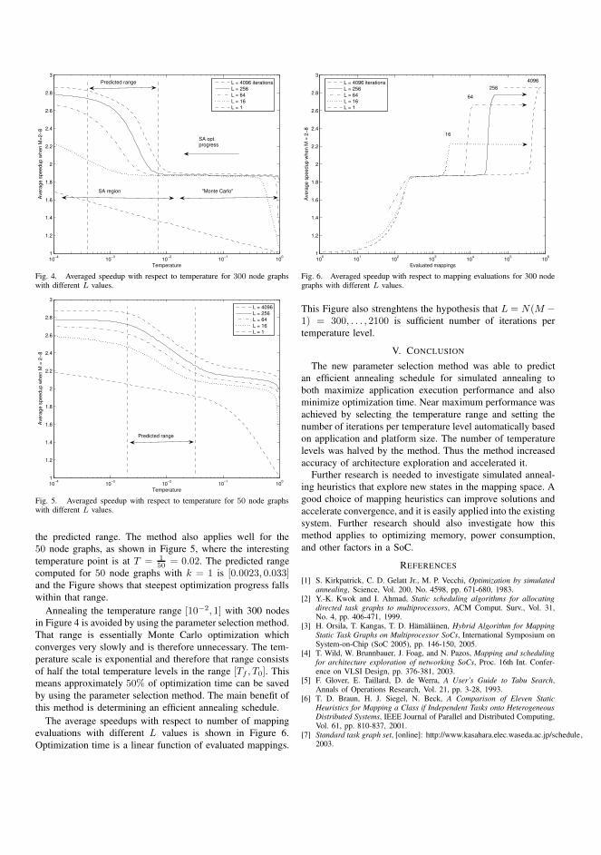
10−4 10−3 10−2 10−1 1001
1.2
1.4
1.6
1.8
2
2.2
2.4
2.6
2.8
3
Temperature
Ave
rage
spe
edup
whe
n M
=2−8
L = 4096 iterationsL = 256L = 64L = 16L = 1
SA opt.progress
"Monte Carlo"SA region
Predicted range
Fig. 4. Averaged speedup with respect to temperature for 300 node graphswith different L values.
10−4 10−3 10−2 10−1 1001
1.2
1.4
1.6
1.8
2
2.2
2.4
2.6
2.8
3
Temperature
Ave
rage
spe
edup
whe
n M
= 2
−8
L = 4096L = 256L = 64L = 16L = 1
Predicted range
Fig. 5. Averaged speedup with respect to temperature for 50 node graphswith different L values.
the predicted range. The method also applies well for the50 node graphs, as shown in Figure 5, where the interestingtemperature point is at T = 1
50 = 0.02. The predicted rangecomputed for 50 node graphs with k = 1 is [0.0023, 0.033]and the Figure shows that steepest optimization progress fallswithin that range.
Annealing the temperature range [10−2, 1] with 300 nodesin Figure 4 is avoided by using the parameter selection method.That range is essentially Monte Carlo optimization whichconverges very slowly and is therefore unnecessary. The tem-perature scale is exponential and therefore that range consistsof half the total temperature levels in the range [Tf , T0]. Thismeans approximately 50% of optimization time can be savedby using the parameter selection method. The main benefit ofthis method is determining an efficient annealing schedule.
The average speedups with respect to number of mappingevaluations with different L values is shown in Figure 6.Optimization time is a linear function of evaluated mappings.
100 101 102 103 104 105 1061
1.2
1.4
1.6
1.8
2
2.2
2.4
2.6
2.8
3
Evaluated mappings
Ave
rage
spe
edup
whe
n M
= 2
−8
L = 4096 iterationsL = 256L = 64L = 16L = 1
16
64
2564096
Fig. 6. Averaged speedup with respect to mapping evaluations for 300 nodegraphs with different L values.
This Figure also strenghtens the hypothesis that L = N(M −1) = 300, . . . , 2100 is sufficient number of iterations pertemperature level.
V. CONCLUSION
The new parameter selection method was able to predictan efficient annealing schedule for simulated annealing toboth maximize application execution performance and alsominimize optimization time. Near maximum performance wasachieved by selecting the temperature range and setting thenumber of iterations per temperature level automatically basedon application and platform size. The number of temperaturelevels was halved by the method. Thus the method increasedaccuracy of architecture exploration and accelerated it.
Further research is needed to investigate simulated anneal-ing heuristics that explore new states in the mapping space. Agood choice of mapping heuristics can improve solutions andaccelerate convergence, and it is easily applied into the existingsystem. Further research should also investigate how thismethod applies to optimizing memory, power consumption,and other factors in a SoC.
REFERENCES
[1] S. Kirkpatrick, C. D. Gelatt Jr., M. P. Vecchi, Optimization by simulatedannealing, Science, Vol. 200, No. 4598, pp. 671-680, 1983.
[2] Y.-K. Kwok and I. Ahmad, Static scheduling algorithms for allocatingdirected task graphs to multiprocessors, ACM Comput. Surv., Vol. 31,No. 4, pp. 406-471, 1999.
[3] H. Orsila, T. Kangas, T. D. Hamalainen, Hybrid Algorithm for MappingStatic Task Graphs on Multiprocessor SoCs, International Symposium onSystem-on-Chip (SoC 2005), pp. 146-150, 2005.
[4] T. Wild, W. Brunnbauer, J. Foag, and N. Pazos, Mapping and schedulingfor architecture exploration of networking SoCs, Proc. 16th Int. Confer-ence on VLSI Design, pp. 376-381, 2003.
[5] F. Glover, E. Taillard, D. de Werra, A User’s Guide to Tabu Search,Annals of Operations Research, Vol. 21, pp. 3-28, 1993.
[6] T. D. Braun, H. J. Siegel, N. Beck, A Comparison of Eleven StaticHeuristics for Mapping a Class if Independent Tasks onto HeterogeneousDistributed Systems, IEEE Journal of Parallel and Distributed Computing,Vol. 61, pp. 810-837, 2001.
[7] Standard task graph set, [online]: http://www.kasahara.elec.waseda.ac.jp/schedule,2003.

108 Publication 2

PUBLICATION 3
H. Orsila, T. Kangas, E. Salminen, M. Hannikainen, T. D. Hamalainen, AutomatedMemory-Aware Application Distribution for Multi-Processor System-On-Chips, Jour-nal of Systems Architecture, Volume 53, Issue 11, ISSN 1383-7621, pp. 795-815,2007.
Copyright 2007 Elsevier B.V. Reproduced with permission.
Automated memory-aware application distributionfor Multi-processor System-on-Chips
Heikki Orsila a,*, Tero Kangas b, Erno Salminen a,Timo D. Hamalainen a, Marko Hannikainen a
a Tampere University of Technology, Institute of Digital and Computer Systems, PO Box 553, FIN-33101 Tampere, Finlandb Nokia Technology Platforms, Visiokatu 6, 33720 Tampere, Finland
Received 22 December 2005; received in revised form 13 November 2006; accepted 15 January 2007Available online 14 February 2007
Abstract
Mapping of applications on a Multi-processor System-on-Chip (MP-SoC) is a crucial step to optimize performance,energy and memory constraints at the same time. The problem is formulated as finding solutions to a cost function ofthe algorithm performing mapping and scheduling under strict constraints. Our solution is based on simultaneous optimi-zation of execution time and memory consumption whereas traditional methods only concentrate on execution time.Applications are modeled as static acyclic task graphs that are mapped on MP-SoC with customized simulated annealing.The automated mapping in this paper is especially purposed for MP-SoC architecture exploration, which typically requiresa large number of trials without human interaction. For this reason, a new parameter selection scheme for simulatedannealing is proposed that sets task mapping specific optimization parameters automatically. The scheme bounds optimi-zation iterations to a reasonable limit and defines an annealing schedule that scales up with application and architecturecomplexity. The presented parameter selection scheme compared to extensive optimization achieves 90% goodness inresults with only 5% optimization time, which helps large-scale architecture exploration where optimization time is impor-tant. The optimization procedure is analyzed with simulated annealing, group migration and random mapping algorithmsusing test graphs from the Standard Task Graph Set. Simulated annealing is found better than other algorithms in terms ofboth optimization time and the result. Simultaneous time and memory optimization method with simulated annealing isshown to speed up execution by 63% without memory buffer size increase. As a comparison, optimizing only executiontime yields 112% speedup, but also increases memory buffers by 49%.� 2007 Elsevier B.V. All rights reserved.
Keywords: Simulated annealing; Task graph; Memory optimization; Mapping; Multi-processor
1. Introduction
The problem being solved is increasing perfor-mance and decreasing energy consumption of
Multi-processor System-on-Chip (MP-SoC). Toachieve both goals, the overall computation shouldbe distributed for parallel execution. However, thepenalty of distribution is often an increased over-all memory consumption, since multi-processingrequires at least local processor caches or databuffers for maintaining efficient computing. Each
1383-7621/$ - see front matter � 2007 Elsevier B.V. All rights reserved.
doi:10.1016/j.sysarc.2007.01.013
* Corresponding author. Tel.: +35 8407325989.E-mail address: [email protected] (H. Orsila).
Journal of Systems Architecture 53 (2007) 795–815
www.elsevier.com/locate/sysarc

Processing Element (PE) is responsible for perform-ing computations for a subset of application tasks.Smallest memory buffers are achieved by runningevery task on the same PE, but it would not be dis-tributed in that case. Therefore, a trade-off betweenexecution time and memory buffers is needed.On-chip memory is expensive in terms of area andenergy, and thus memory is a new, important opti-mization target.
Application distribution is a problem of mappingtasks on separate processing elements (PEs) for par-allel computation. Several proposals have beenintroduced over the years; the first ones being forthe traditional supercomputing domain. An optimalsolution has been proven to be an NP problem [1],and therefore a practical polynomial time heuristicsis needed. In extreme cases heuristics are either toogreedy to explore non-obvious solutions or notgreedy enough to discover obvious solutions. Mostof the past distribution algorithms are not used tooptimize memory consumption.
In a traditional super-computing domain, opti-mizing performance means also increasing networkusage, which will at some point saturate the networkcapacity and the application performance. For MP-SoC, the interconnect congestion must be modeledcarefully [2,3] so that the optimization methodbecomes aware of network capacity and perfor-mance, and is able to allocate network resourcesproperly for all the distributed tasks.
Simulated annealing (SA) [4,5] is a widely usedmeta-algorithm to solve the application distributionproblem. However, it does not provide a definiteanswer for the problem. Simulated annealingdepends on many parameters, such as move heuris-tics, acceptance probabilities for bad moves, anneal-ing schedule and terminal conditions. Selection ofthese parameters is often ignored in experimentalpapers. Specializations of the algorithm have beenproposed for application distribution, but manycrucial parameters have been left unexplained andundefined. An automated architecture explorationtool using SA requires a parameter selection methodto avoid manual tuning for each architecture andapplication trial. Automated SA parameter selec-tion has not been previously addressed in the con-text of architecture exploration.
This paper presents three new contributions. Thefirst is a new optimization method with a cost func-tion containing memory consumption and executiontime. It selects the annealing schedule, terminal con-ditions and acceptance probabilities to make simu-
lated annealing efficient for the applied case.Second is an automatic parameter selection methodfor SA that scales up with application and systemcomplexity. Third contribution is empirical compar-ison between three mapping algorithms, which areSA, modified group migration (Kernighan–Lingraph partitioning) algorithm and random map-ping. SA without automatic parameter setting isalso compared.
The outline of the paper is as follows. Section 2presents the terminology. Section 3 analyzes prob-lems and benefits of other systems, and comparesthem to our method. Section 4 explains our optimi-zation framework where the method is applied.Section 5 presents our optimization method forautomatic parameter selection and memory optimi-zation. Section 6 presents the scheduling system thatis used for the optimization method. The experi-ment that is used to validate and compare ourmethod to other algorithms is presented in Section7 and the results are presented in Section 8. Section9 justifies the parameter selection method. Andfinally, Section 10 concludes the paper.
2. Terminology
Allocation, mapping and scheduling are phasesin realizing application distribution on MP-SoC.Allocation determines how many and what kindof PEs and other resources there are. Mappingdetermines how the tasks are assigned to the allo-cated PEs. Task scheduling determines the execu-tion order and timing of tasks on each PE, andcommunication scheduling determines the orderand timing of transfers on each interconnect. Theresult of this process is a schedule, which determinesexecution time and memory consumption.
For mapping optimization, the application ismodeled in this paper with static task graphs(STG). STG is a directed acyclic graph (DAG),where each node represents a finite deterministictime computation task. Simulating an applicationmodeled as STG means traveling a directed acyclicgraph from ancestors to all children uncondition-ally. Nodes of the graph are tasks, and edges presentcommunication and data dependence among tasks.
Fig. 1 shows an example of an STG. Weights ofnodes, marked as values inside parenthesis, indicatecomputation costs in terms of execution time. In theexample, node E has computational cost of 5. Eachedge of the graph indicates a data dependency, forexample B is data dependent on A. Weights of
796 H. Orsila et al. / Journal of Systems Architecture 53 (2007) 795–815

edges, marked as numbers attached to edges in thefigure, indicate communication costs associatedwith the edges. The edge from C to F costs fourunits, which are data sizes for communication.The communication time will be determined bythe interconnect bandwidth, its availability and datasize. STGs are called static because connectivity ofthe graph, node weights and edge weights are fixedbefore run-time. Communication costs changebetween runs due to allocation and mapping thusaffecting edge weights.
A relevant factor regarding achievable parallel-ism is the communication to computation ratio(CCR). It is defined as the average task graph edgeweight divided by the average node weight (whenconverted to comparable units). By the definition,CCR over 1.0 means that computation resourcescannot be fully utilized because there is morecommunication than computation to do.
There is no conditional task execution in STG,but having conditional or probabilistic children (inselecting path in the graph) or run-time determinednode weights would not change mapping algorithmsdiscussed in this paper. However, a more complexapplication model, such as a probabilistic model,would make the scheduling problem harder andcomparison of mapping algorithms a very largestudy.
Despite these limitations, STGs could be used tomodel, for example, a real-time MPEG4 encoderbecause real-time systems have bounded executionand communication costs for the worst case behav-ior. Many multimedia applications belong to real-time category and therefore applicability of STGsis wide. STGs are also widely used in related work,which helps comparisons.
Memory consumption of the application is par-tially determined by the STG. It is fully determinedafter the mapping and scheduling have been done. Anode, or its associated PE in practice, must preserveits output data until it has been fully sent to all itschildren. Also, a set of nodes on the same PE mustpreserve input data until computation on all nodesthat require the data are finished. Results or inputdata that are stored for a long period of time willincrease memory buffer usage significantly. Analternative solution for this problem can possiblybe found by task duplication or resending results.However, task duplication increases PE usage andresending results increases interconnect congestion,for which reason we do not consider these tech-niques in this paper. Results are sent only onceand they are preserved on the target PE as long asthey are needed. The results are discarded immedi-ately when they are not needed. Thus memory con-sumption depends heavily on the mapping andscheduling of the application.
3. Related work
Many existing optimization methods use stochas-tic algorithms such as SA [4,5] and genetic algo-rithms [6,7]. These algorithms have been appliedon wide variety of hard optimization problems,but there is no consensus or common rules how toapply them on MP-SoC optimization. SA can beused with any cost function, but it is a meta-algo-rithm because parts of it have to be specializedfor any given problem. The relevant mathematicalproperties for this paper are discussed in [19]. SAhas been applied to many challenging problems,including traveling salesman problem [4], and map-ping and scheduling of task graphs [8].
Wild et al. [2] compared SA, Tabu Search [9] andvarious algorithms for task distribution to achievespeedup. Their results showed 7.3% advantage forTabu Search against SA, but they also stated theywere not able to control the progress of SA. Theirpaper left many SA parameters undefined, such asinitial temperature, final temperature, maximumrejections and acceptance function, which raisesquestions about accuracy of the comparison withrespect to SA. Their method uses SA with geometrictemperature schedule that decreases temperatureproportionally between each iteration until a finaltemperature is reached and then optimization is ter-minated. As a consequence the number of iterationsis fixed for a given initial temperature, and thus, the
A (1)B (2)1
E (5)
1
F (6)
2
C (3)
4D (4)
11
Fig. 1. Example of a static task graph. Values in parenthesisinside the nodes represent execution time, and values at edgesrepresent communication sizes. The communication time will bedetermined by the interconnect, its availability and data size.
H. Orsila et al. / Journal of Systems Architecture 53 (2007) 795–815 797

method does not scale up with application and sys-tem complexity.
Our method increases the number of iterationsautomatically when application and system com-plexity grows, which is more practical and lesserror-prone than setting parameters manually formany different scales of problems. The common fea-ture for our and Wild et al. is the use of dynamicallyarbitrated shared bus with multiple PEs, as well asfirst mapping task graphs and then scheduling witha B-level scheduler. Their system is different in hav-ing HW accelerators in addition to PEs, and theydid not present details about HW accelerator per-formance or CCR values of the graphs they used.Our paper focuses on CCR values in the range[0.5, 1.0], because computation resources are notwasted too much in that range, and it is also possi-ble to achieve maximum parallelism in some cases.
Braun et al. [10] compared 11 different optimiza-tion algorithms for application distribution. Theyalso compared Tabu Search and SA, and in theirresults, comparing to results from Wild et al., SAwas better than Tabu Search in three out of sixcases. Genetic algorithms gave the best results intheir experiment. Their SA method had a benefitof scaling up with application complexity in termsof selecting initial temperature with a specificmethod. Our approach has the same benefit imple-mented with a normalization factor integrated intoto acceptance probabilities.
The number of iterations in Braun’s method doesnot scale up correctly because it is not affected bythe number of tasks in application. As a bad sideeffect of their initial temperature selection method,the number of iterations for SA is affected by theabsolute time rather than relative time of applica-tion tasks. This is avoided in our method by usinga normalized temperature scale, which is made pos-sible by the normalization factor in our acceptanceprobability function. Braun’s annealing schedulewas a geometric temperature with 10% temperaturereduction on each iteration, implying that the tem-perature decreases fast. This has the consequencethat one thousandth of initial temperature isreached in just 87 iterations, after which the optimi-zation is very greedy. Thus, the radical explorationphase in SA, which means high temperatures, isnot dependent on application complexity, andtherefore the exploration phase may be too shortfor complex applications. Their method also lacksapplication adaptability because the maximumrejections has a fixed value of 150 iterations regard-
less of the application complexity. They usedrandom node (RN) heuristics for randomizing newmappings, which is inefficient with small amountof PEs as described in Section 5.2.
Spinellis [11] showed an interesting SA approachfor optimizing production line configurations inindustrial manufacturing. Obviously the two fieldsare very different in practice, but theoretical prob-lems and solutions are roughly the same. As a spe-cial case, both fields examine the task distributionproblem to gain efficiency. Spinellis showed anautomatic method for SA to select the number ofiterations required for a given problem. Theirmethod scaled up the number of iterations for eachtemperature level based on the problem size. Asimilar method is used in our method for task distri-bution. Unfortunately acceptance probabilities,meaning the dynamic temperature range, were notnormalized to different problems.
Our paper presents a specialization of the SAmeta-algorithm that addresses SA specific problemsin previously mentioned papers. Initial temperature,final temperature and acceptance probabilities arenormalized to standard levels by an automaticmethod that scales up both with application andallocation complexity. Furthermore, the total opti-mization effort is bounded by a polynomial functionthat depends on application and allocationcomplexity.
Group Migration (GM), also known as Kerni-ghan–Lin algorithm, is a very successful algorithmfor graph partitioning [12]. It has been comparedto SA in [22] and suggested to be used for task map-ping in [14]. Mapping is done by partitioning thetask graph into several groups of tasks, each groupbeing one PE. The algorithm was originallydesigned to partition graphs into two groups, butour paper uses a slightly modified version of thealgorithm for arbitrary number of groups while pre-serving the old behavior for two groups. The idea tomodify the algorithm is presented in [14] and anexample is presented in [15].
Sinnen and Sousa [3] presented an applicationmodel that embeds the interconnect structure andcontention into the optimization process. They pre-sented a method to schedule communication onto aheterogeneous system. Wild et al. [2] showed a sim-ilar scheduling method to insert communicationsonto a network to optimize communications. Taskgraphs in their paper had 0.1, 1.0 and 10.0 as CCRs.They concluded that CCR of 10.0 was too challeng-ing to be distributed and that effect of communica-
798 H. Orsila et al. / Journal of Systems Architecture 53 (2007) 795–815

tion congestion model is quite visible already in theCCR value of 1.0. These findings support our simi-lar experience. Our method also schedules commu-nications based on priorities of tasks that willreceive communication messages.
Also, Sinnen and Sousa [16] modeled side-effectsof heavy communication in SoCs by adding com-munication overhead for PEs. Most parallel systemmodels are unaware of PE load caused by commu-nication itself. For example TCP/IP systems needto copy data buffers from kernel to applicationmemory. Sinnen and Sousas model is insufficient,however, because it does not model behavior ofinterrupt-driven and DMA-driven communication,which are the most common mechanisms for highperformance computing. Communication overheadshould be extended over execution of multiple pro-cesses in a normal case of interrupt driven com-munication. In order to avoid bias of specificapplications, our model does not have processoroverhead for communication. Our model assessespotential of various mapping algorithms rather thaneffects of communication model.
Other approaches for the performance, memoryand power optimization include task graph parti-tioning to automatically select system architecturefor a given application. Hou et al. [25] presented amethod for partitioning task graph onto a suitablearchitecture. The system presented in this paperdoes not partition task graphs, but the method in[25] is directly applicable to our optimization systemas well.
Szymanek et al. [17] presented an algorithm tosimultaneously speedup executing and optimizememory consumption of SoC applications. Theirmethod keeps track of data and program memoryrequirements for different PEs to achieve the goal.It is based on constraint programming that setshard limits on memory and time requirements,whereas our method only places relative cost onmemory and time but allows all solutions.
Panda et al. [24] optimized the memory architec-ture to fit a given application. This paper’s approachpenalizes using memory on the application levelwhile optimizing for performance. Methods dis-cussed in [24] could be applied to the system pre-sented in this paper as well. Their method operateson the system level and ours on the applicationlevel.
Kwok et al. did a benchmark on various schedul-ing algorithms [13] and they explained methods andtheory of the same algorithms in [18]. We chose B-
level scheduling policy for our method, because itwas a common element in well performing schedul-ing algorithms. The MPC algorithm was the bestscheduling policy in their benchmark on thebounded number of processors case, and it is basedon the B-level scheduling.
Ascia et al. [23] used genetic algorithms to mapapplications onto a SoC obtaining a pareto-frontof solutions for multiple cost functions. Their systemallows the designer to choose the best solution frommultiple controversial design goals. Their goal is,however, different than ours, because our systemneeds to pick a single good solution as part of anautomated CAD system [26]. Other than that,multi-objective optimization and genetic algorithmswould fit well into the system presented in this paper.
4. MP-SoC application distribution framework
Our MP-SoC application distribution frameworkis shown in Fig. 2. The optimization process startsby selecting an allocation and an application, whichare target hardware and a task graph. Allocationand the application are passed to a mapping algo-rithm. The mapping algorithm is chosen betweengroup migration, random mapping or SA. The algo-rithm starts with an initial solution in which all taskgraph nodes are mapped to a single PE and theniterates through various mapping candidates to finda better solution. The mapping candidates are
Allocation
Mapping
Scheduling
Cost evaluation
Results
Application
Platform library
Allocationcandidate
Mappingcandidate
Schedulingcandidate
Application distribution Contents of this paper
• HIBI MP-SoC network• Generic PE models
• Static task graphs from the Standard Task Graph Set
• 1-4 PEs• Fixed width shared bus
• Simulated annealing• Group Migration• Random
• B-level scheduler
• Application execution time• Application memory consumption• Optimization time• Number of iterations
• Time-Memory objective function
Fig. 2. MP-SoC application distribution framework.
H. Orsila et al. / Journal of Systems Architecture 53 (2007) 795–815 799

scheduled with a B-level scheduler to determine theexecution time and memory usage. The B-levelscheduler decides the execution order for each taskon each PE to optimize execution time. The good-ness of the candidate is evaluated by a cost functionthat depends on the execution time and memoryconsumption. At some point mapping algorithmstops and returns the final mapping solution.
In many optimization systems mapping andscheduling are dependent on each other [18], butin this system allocation, mapping and schedulingalgorithms can be changed independently of eachother to speedup prototyping of new optimizationalgorithms. The current system allows optimizationof any task-based system where tasks are mappedonto PEs of a SoC consisting of arbitrary intercon-nection networks. Therefore, dynamic graphs andcomplex application models can be optimized aswell. Communication delays and the interconnec-tion network can vary significantly and thus sched-uling is separated from mapping. Communicationdelays for both shared and distributed memoryarchitectures can be modeled as well.
The system uses a single cost function, butmulti-objective systems analyzing pareto-fronts ofmultiple solutions [23] could implemented withoutaffecting the optimization algorithms presentedhere.
5. Mapping algorithms
5.1. Simulated annealing algorithm
The pseudo-code of the SA algorithm is pre-sented in Fig. 3, and explanations of symbols aregiven in Table 1. SA cannot be used for task map-ping without specializing it. The following parame-ters need to be chosen for a complete algorithm:annealing schedule, move heuristics, cost function,acceptance probability and the terminal condition.
The Cost function in Fig. 3 evaluates the cost forany given state of the optimization space. Eachpoint in the optimization space defines a mappingfor the application. The optimization loop is termi-nated after Rmax amount of consecutive moves thatdo not result into improvement in cost. The Temper-
ature-Cooling function on Line 7 determines theannealing rate of the method which gets two param-eters: T0 is the initial temperature, and i is the iter-ation number. The Move function on Line 8 is amove heuristics to alter current mapping. It dependson the current state S and temperature T. The Ran-
dom function returns a random number from theuniform probability distribution in range [0, 1).The Prob function determines the probability foraccepting a move to a worse state. It depends onthe current temperature and the increase of costbetween old and new state.
Fig. 3. Simulated annealing algorithm.
Table 1Summary of symbols of the simulated annealing pseudo-code
C Cost function valueCbest Best cost function valueCost() Cost functioni Iteration numberMove() Move heuristics functionp Probability valueProb() Probability function of accepting a bad
mover Random valueRandom() Random variable function returning value in
range [0, 1)R Number of consecutive move rejectionsRmax Maximum number of rejectionsS Optimization state (mapping)S0 Initial stateSbest Best stateT Current temperature in range (0, 1]T0 Initial temperature (1.0 in this method)Tf Final temperatureTemperature-
Cooling()Annealing schedule function
800 H. Orsila et al. / Journal of Systems Architecture 53 (2007) 795–815

5.2. Automatic parameter selection for SA
The choice of annealing schedule (Temperature-
Cooling function) is an important factor for optimi-zation [19]. Mathematical theory establishes thatinfinite number of iterations is needed to find a glo-bal optimum with SA. However, the mapping prob-lem is finite but it is also an NP problem implyingthat a practical compromise has to be made thatruns in polynomial time. Annealing schedule mustbe related to the terminal condition. We define the
dynamic temperature scale to be r ¼ log T 0
T f
� �and
assert that a terminal condition must not be truebefore a large scale of temperatures has been tried,because only a large scale r allows careful explora-tion of the search space. High temperatures willdo rapid and aggressive exploration, and low tem-peratures will do efficient and greedy exploration.A common choice for the annealing schedule is afunction that starts from an initial temperature,and the temperature decreases proportionallybetween each level until the final temperature isreached. The proportion value p is close to but smal-ler than 1. Thus the number of temperature levels isproportional to r. We will use this schedule.
The terminal condition of annealing must limitthe computational complexity of the algorithm sothat it is reasonable even with larger applications.The maximum number of iterations should growas a polynomial number of problem factors ratherthan as an exponential number that is required fortrue optimum solution. The relevant factors forthe number of iterations are initial temperature T0,final temperature Tf, the number of tasks to bemapped N and the number of PEs M.
Further requirement for task mapping is thatannealing schedule must scale with application andallocation complexity with respect to optimizationability. This means that the amount of iterationsper temperature level must increase as the appli-cation and allocation size grows. For N tasks andM PEs one must choose a single move fromN(M � 1) different alternatives, and thus it is logicalthat the amount of iterations per temperature levelis at least proportional to this value. Consideringthese issues we define the system complexity as
L ¼ NðM � 1Þ ð1ÞThus the complexity measure is a product of appli-cation and allocation complexity. Furthermore werequire that the number of iterations for each tem-perature level is L, because that is the number of
choices for changing a single mapping on any givenstate. Also, we select the number of temperaturelevels according to dynamic temperature scale r.
It must be noted that SA will very unlikely tryeach alternative mapping for a temperature leveleven if the number of iterations is L because theheuristics move is a random function. Also, if amove is accepted then the mapping alternatives afterthat are based on the new state and therefore tryingL different alternatives will not happen. In the caseof frequent rejections due to bad states or lowtemperature, the L amount of moves gives similarbehavior as the group migration algorithm, butnot exactly the same because SA makes chains ofmoves instead of just trying different move alter-natives. Also, SA does not share the limitations ofgroup migration because it is not greedy until lowtemperature levels are reached.
The chosen terminal condition is true when thefinal temperature is reached and a specific amountof consecutive rejections happen. The maximumamount of consecutive rejections Rmax should alsoscale with system complexity, and therefore it ischosen so that Rmax = L.
Based on these choices we get a formula to com-pute the total number of iterations for SA. Thenumber of different temperature levels x in Eq. (2)depends on the proportion p and the initial and finaltemperatures as
T 0px ¼ T f ) x ¼log T f
T 0
log p: ð2Þ
The total number of iterations Itotal is computed inEq. (3) based on the number of different tempera-ture levels x and the number of tasks and PEs ofthe system as
I total ¼ xLþ Rmax ¼ xLþ L ¼ ðxþ 1ÞL
¼log T f
T 0
log pþ 1
!NðM � 1Þ ð3Þ
Therefore, the total number of iterations is a func-tion of N tasks, M PEs and the temperature scale r.
Eq. (4) shows the annealing schedule functiondecreasing temperature geometrically every L itera-tions as
Temperature-CoolingðT 0; iÞ ¼ T 0piLb c: ð4Þ
A common choice for acceptance probability isshown in Eq. (5) as
H. Orsila et al. / Journal of Systems Architecture 53 (2007) 795–815 801

Basic-ProbabilityðDC; T Þ ¼ 1
1þ exp DCT
: ð5Þ
DC is the increase in cost function value betweentwo states. A bigger cost increase leads to lowerprobability, and thus moving to a much worse stateis less probable than moving to a marginally worsestate. The problem with this function is that it givesa different probability scale depending on the scaleof the cost function values of a specific system.The system includes the platform and applications,and it would be a benefit to automatically tune theacceptance probability to the scale of the costfunction.
We propose a solution to normalize the probabil-ity scale by adding a new term to the expressionshown in Eq. (6). C0 is the initial cost function valueof the optimization process. The term DC
C0makes the
state change probability relative to the initial costC0. This makes annealing comparable between dif-ferent applications and cost functions. An addi-tional assumption is that temperature T is in range(0, 1].
Normalized-ProbabilityðDC; T Þ ¼ 1
1þ exp DC0:5C0T
ð6ÞFig. 4 presents acceptance probabilities for the nor-malized probability function for relative cost func-tion changes and temperatures. The probabilitieslie in the range (0, 0.5]. As the relative cost changegoes to zero, the probability goes to 0.5. Thus thefunction has a property of easily allowing SA totake many small steps that have only a minor wors-
ening effect on the cost function. When the temper-ature decreases to near zero, these small worseningsteps become very unlikely.
A common choice for move heuristics [2,6,10] is afunction that chooses one random task and mapsthat to a random PE. It is here named as the RN(Random Node) move heuristics and presented inFig. 5. It has the problem that it may do unneces-sary work by randomizing exactly the same PEagain for a task. In 2 PE allocation case probabilityfor that is 50%. Despite this drawback, it is a verycommon choice as a move heuristics.
The obvious deficiency in the RN heuristics isfixed by our RM move (Random Modifying move)heuristics presented in Fig. 6. It avoids choosing thesame PE and, thus, has a clear advantage over theRN heuristics when only a few PEs are used. Thissmall detail has often been left unreported on otherpublications, but it is worth pointing out here.
Fig. 7 shows an example of annealing process foroptimizing execution time of a 50 node STG on 2PEs. The effect of annealing from high temperatureto a low temperature can be seen as the cost func-tion altering less towards the end. At the end theoptimization is almost purely greedy, and henceallows moves to a worse state with a very low prob-ability. This figure shows the cost function value ofthe current accepted state rather than cost functionvalues of all tried states. A figure showing cost func-tion values of all tried states would be similar to awhite noise function.
5.3. Group migration algorithm
Group migration is used to map task graphs ontomultiple PEs in a greedy fashion. This is a general-
10 10 10 10 100
4 3 2 1 0
0.05
0.1
0.15
0.2
0.25
0.3
0.35
0.4
0.45
0.5
ΔCr = 0.0001
ΔCr = 0.0010
ΔCr = 0.0100
ΔCr = 0.1000
ΔCr = 1.0000
Temperature
etatsesro
wot
evom
afoytilibaborp
ecnatpeccA
Fig. 4. Acceptance probabilities for the normalized probabilityfunction with respect to relative cost function change DCr ¼ DC
C0.
Fig. 5. RN move heuristics moves one random task to a randomPE.
Fig. 6. RM move heuristics moves one random to a differentrandom PE.
802 H. Orsila et al. / Journal of Systems Architecture 53 (2007) 795–815

ization of the original algorithm [12] that parti-tioned graphs to two disjoint subsets. Our modifiedversion partitions the graph into arbitrarily manydisjoint subsets.
The algorithm is greedy because it only acceptsmoves to better positions, and thus it always getsstuck into a local minimum in the optimizationspace. The algorithm consists of migration rounds.Each round either improves the solution or keepsthe original solution. Optimization ends when thelatest round is unable to improve the solution. Usu-ally the algorithm converges into a local minimumin less than five rounds [12].
A move in GM means moving one specific taskto another PE. A round consists of sub-roundswhich try all tasks on all other PEs. With N nodesand M PEs it is (M � 1)N tries. The best move onthe sub-round is chosen for the next sub-round.Tasks, which have been moved as best task candi-dates on previous sub-rounds, are not movedanymore until the next round comes. There areat most N sub-rounds. This results into at most(M � 1)N2 moves per round. If no improving moveis found on a sub-round, the round is terminated,because all possible single moves were already tried((M � 1)N tries). The pseudo-code of the modifiedgroup migration algorithm is shown in Fig. 8 and
variables that are new compared to SA areexplained in Table 2.
The main loop of the pseudo-code begins on Line1 of Group-Migration function. It calls GM-Round
function as long as it can improve the mapping.GM-Round will change at most one mapping perround. If it does not change any, the optimizationwill terminate. GM-Round first computes the initialcost of initial state S0 on Line 2. The Cost functionis the same function as with SA. Line 3 initializesan array that marks all tasks as non-moved. Thefunction can only move each task once from onePE to another, and this table keeps record of tasksthat have been moved. Moved tasks can not bemoved again until the next call to this function.The upper limit of loop variable i on Line 4 signifiesthat each task can only be moved once. Increasingthe upper limit would not break or change the func-tional behavior. Line 7 begins a sub-round whichends at Line 20. The sub-round tries to move eachtask from one PE to every other PE. The algorithmaccepts a move on Line 15, if it is better than anyother previous move. The effect of any previousmoves is discarded on Line 19, even if a moveimproved mapping. However, the best improvingmove is recorded for later use on Lines 17–18. Eachmove is a separate try that ignores other moves. If no
0 1000 2000 3000 4000 5000 6000 7000 8000 9000 100001
1.2
1.4
1.6
1.8
2
2.2x 10
Mapping iteration
AS rof tsoc detpecc
ACostBest costLocal minimum
Fig. 7. An example of annealing from a high to a low temperature state for a 50 node STG with 2 PEs. · marks the mapping iteration thathas the lowest cost function value.
H. Orsila et al. / Journal of Systems Architecture 53 (2007) 795–815 803

improving move was found in the loop beginning onLine 7, the search is terminated for this round onLine 21. Otherwise, the best move is applied on Lines23–24. The best found is returned on Line 25.
5.4. Random mapping algorithm
Random mapping is an algorithm that selects arandom PE separately for all tasks on every invoca-
tion of the algorithm. The algorithm is a usefulbaseline comparison algorithm [14] against otheralgorithms since it is a policy neutral mapping algo-rithm that converges like Monte Carlo algorithms.The random mapping exposes the inherent parallel-izability of any given application for a given numberof iterations. It should be compared with other algo-rithms by giving the same number of iterationsfor both algorithms. Random mapping results arepresented here to allow fair comparison of the SAand GM methods against any other mappingalgorithms. Cost function ratio of SA and randommapping can be compared to the ratio of any otheralgorithm and random mapping.
6. Scheduling and cost functions
6.1. B-level scheduler
The scheduler decides the execution order oftasks on each PE. If a task has not been executedyet, and it has all the data required for its execution,it is said to be ready. When several tasks are readyon a PE the scheduler selects the most importanttask to be executed first.
Tasks are abstracted as nodes in task graphs, andcommunication is abstracted as edges. Node andedge weights, which are cycle times and data sizes,respectively, are converted into time units beforescheduling. The conversion is possible because allo-cation and mapping are already known.
The scheduler applies B-level scheduling policyfor ordering tasks on PEs. The priority of a nodeis its B-level value [18]. Higher value means moreimportant. The B-level value of a node is the longestpath from that node to an exit node, including exitnodes weight. Exit node is defined as a node that hasno children. The length of the path is defined as thesum of node and edge weights along that path. Forexample, in Fig. 1 the longest path from A to F is1 + 1 + 5 + 1 + 6 = 14, and thus B-level value ofnode A is 14.
As an additional optimization for decreasingschedule length, the edges, which represent commu-nication, are also scheduled on the communicationchannels. A priority of an edge is the weight ofthe edge added with B-level values of child nodes.Thus, children who have higher priority may alsoreceive their input data more quickly.
Fig. 9 shows pseudo-code for computing B-levelpriorities for an STG. Line 1 does a topological sorton the task graph. The topological sort means
Fig. 8. A modified group migration algorithm for arbitrarynumber of PEs.
Table 2Summary of new variables used in the group migration algorithm
A PEAold Old PEDPE PE associated with the best migration candidateDtask Task associated with the best migration candidateMoved Array of Booleans indicating tasks that have been
moved
804 H. Orsila et al. / Journal of Systems Architecture 53 (2007) 795–815

ordering the task graph into a list where the node Ais before the node B if A is a descendant of B. Thusthe list is ordered so that children come first. Line 2iterates through all the tasks in that order. Line 3sets default B-level value for a node, which is onlyuseful if the node is an exit node. Array B containsknown B-level values so far. If a node is not an exitnode, the B-level is computed on Lines 4–9 to be themaximum B-level value with respect to its children.A B-level value with respect to a child is the sum ofchild’s B-level value, edge weight towards the child,and the node weight of the parent node.
It should be noted that although B-level value isdependent on communication costs, it does notmodel communication congestion. Despite thislimitation, Kwok et al. show in [13] that the bestbounded number of processor (BNP) class schedul-ing algorithm is based on ALAP (as late as possible)time. ALAP time of a node is defined as the differ-ence of the critical path length and the B-level valueof the node. An unscheduled node with the highestB-level value is by definition on the dynamic criticalpath, and therefore B-level priority determinesALAP time uniquely, and therefore B-level priorityis an excellent choice.
The algorithmic complexity of the B-level prior-ity computation is O(E + V), where E is the numberof edges and V is the number of nodes. However,the list scheduling algorithm complexity isO((E + V)log V), which is higher than the complex-ity of computing B-level priorities, and therefore thecomplexity of the whole scheduling system isO((E + V)log V).
6.2. Cost function
In this paper, the optimization process measurestwo factors from a mapped system by scheduling the
task graph. Execution time T and memory buffersize S are the properties which determine the costfunction value of a given allocation and mapping.
The scheduler system simulates the task graphand architecture by executing each graph node par-ent before the child node is executed as well asdelaying the execution of the child node until resultsfrom the parent nodes have arrived, thus determin-ing the execution time T by behavioral simulation.The system is, however, not limited to behavioralsimulation, but exact models on the underlyingsystem could be used by changing the schedulerpart.
The scheduler keeps track of buffers that areneeded for the computation and communicationto determine memory buffer size S. When a PEstarts receiving a data block from another PE itneeds to allocate a memory buffer to contain thatdata. The PE must preserve that data buffer as longas it is receiving the data or computing somethingbased on that data. The receiving buffer is freedafter the computation. When a PE starts computingit needs to allocate memory for the result. The resultis freed when the computation is done and the resulthas been sent to other PEs.
As a result, when the full schedule of an STG hasbeen simulated, the scheduler knows memory size Srequired for the whole architecture and the totalexecution time T. The mapping algorithm is orthog-onal to the scheduler part in our system, which wasthe design goal of the optimization framework, andthus other optimization parameters could be easilyadded by just changing the scheduler part withoutaffecting the mapping algorithms.
The cost function is chosen to optimize both exe-cution time and required memory buffers, that is,minimize the cost function aT + bS, where a and b
are constants. When both time and memory areoptimized, parameters a and b are chosen so thaton a single PE case both aT and bS are 0.5 and thuscost function has the value 1.0 in the beginning.
The motivation for including memory buffer sizefactor into the cost function is to minimize expen-sive on-chip buffer memory required for parallelcomputation. An embedded system designer maybalance cost function factors to favor speedup ormemory saving depending on which is more impor-tant for the given application. Adding more factorsinto the cost function will motivate for researchon multi-objective optimization and can takeadvantage of pareto-optimization methods such as[23].
Fig. 9. Algorithm to compute B-level values for nodes of a taskgraph.
H. Orsila et al. / Journal of Systems Architecture 53 (2007) 795–815 805

7. Experiments
7.1. Setup for the experiment
The optimization software is written for theUNIX environment containing 3600 lines of C code.On a 2.0 GHz AMD Athlon 64 computer, the soft-ware is able to evaluate 12,000 mappings in a secondfor a 50 node STG with 119 edges, or 600,000 nodesor 1.43 million edges in a second. The software did2094 mappings in a second for a 336 node STG with1211 edges, or 703,584 nodes or 2.54 million edgesin a second. Thus the method scales well with thenumber of nodes and edges. Scalability follows fromthe computational complexity of the schedulingmethod because a single mapping iteration withoutscheduling is in O(1) complexity class.
The experiment is divided into two categories.The first category is the execution time optimiza-tion, where the cost function is the execution timeof the application. The second category is the execu-tion time and memory buffer optimization, wherethe cost function is a combination of execution timeand memory buffers. Both categories are tested withSA, GM and random mapping algorithms. Eachalgorithm is used with 1 to 4 PEs. The single PE caseis the reference case that is compared with otherallocations. For each allocation, 10 graphs with 50nodes and 10 graphs with 100 nodes are tested.The graphs were random STGs with randomweights. Each graph is optimized 10 times with
exactly the same parameters. Thus, the total amountof optimizations is 2 (categories) * 3 (algorithms) *3 (PE allocations) * 20 (STGs) * 10 (independentidentical runs) = 3600 runs. Fig. 10 depicts thewhole experiment as a tree. Only one branch oneach level is expanded in the figure, and all branchesare identical in size.
7.2. Simulated annealing parameters
SA parameters are presented in Table 3. Finaltemperature is only 0.0001, and therefore SA is verygreedy at the end of optimization as shown by theacceptance function plot in Fig. 4.
Table 4 shows the total number of mappings forone SA descend based on the parameters shown inTable 3.
7.3. Group migration and random mapping
parameters
Group migration algorithm does not need anyparameters. This makes it a good algorithm to com-pare against other algorithms because it is also easyto implement and suitable for automatic architec-ture exploration. Relative advantage of the SAmethod over GM can be compared to any otheralgorithm over GM.
Experiment
Time Time + Memory
SA
1 PE 4 PEs
50 Node STG 100 Node STG
STG 1 STG 10
Run 1 Run 10
. . . .
. . . .
GMRANDOM
. . . .
Fig. 10. Outline of the experiment procedure.
Table 3Parameters for simulated annealing
Temperatureproportion (p)
0.95
Initial temperature (T0) 1.0Final temperature (Tf) 0.0001Iterations per
temperature levelL = N(M � 1) (Eq. (1))
Move heuristics RM-moveAnnealing schedule
(Temperature-Cooling)
Temperature decreasesproportionally once in L iterations
Acceptance probability(Prob)
Normalized probability (Eq. (6))
Terminal condition Final temperature is reached and atleast L consecutive rejections areobserved
Table 4Total number of mappings for one simulated annealing descend
2 PEs 3 PEs 4 PEs
52 tasks 9300 18,700 28,000102 tasks 18,300 36,600 54,900
806 H. Orsila et al. / Journal of Systems Architecture 53 (2007) 795–815

Random mapping tries N2M2 random mappingsindependently, which is much more than with SA.Random mapping is defined as choosing a randomPE separately for all tasks. Random mapping pre-sents a neutral reference to all other algorithms bothin terms of behavior and efficiency. It does worsethan other algorithms, as experiment will show,but it shows how much can be optimized withoutany knowledge of system behavior.
7.4. Static task graphs
STGs used in this paper are from Standard TaskGraph Set [20]. The experiment uses 10 randomSTGs with 50 nodes and 10 random STGs with100 nodes. The task graph numbers from 50 nodegraphs are: 2, 8, 18, 37, 43, 49, 97, 124, 131 and146. The task graph numbers from 100 node graphsare: 0, 12, 15, 23, 46, 75, 76, 106, 128 and 136. Edgeweights had to be added into the graphs because theStandard Task Graph collection graphs do not havethem. In this case study, each edge presents commu-nication of Normal(64, 162) bytes. That is, the edgeweights are normally distributed with mean of64 bytes and standard deviation of 16 bytes. Thenode weights were multiplied by a factor of 32 tohave communication to computation ratio (CCR)at a reasonable level. The CCR is defined as theaverage edge weight divided by the average nodeweight. Summary of the properties is presented inTable 5.
7.5. MP-SoC execution platform
The MP-SoC execution platform on which exper-iments are run is assumed to have a number of iden-tical PEs as shown in Fig. 11. Each PE is a 50 MHzgeneral purpose processor (GPP), and thus it canexecute any type of task from the TG and the map-ping space does not have constraints. Task execu-tion on a GPP is uninterruptible by the othertasks. IO operations are carried out in the back-ground and they are assumed to be interrupt-driven.
Task execution time is one or more GPP cycles. Thisis converted into time units by dividing the cyclenumber by the associated PE’s clock frequencybefore scheduling.
The PEs are connected with a single dynamicallyarbitrated shared bus, and all the PEs are equallyarbitrated on the bus. Transaction is defined astransferring one or more data words from one PEto another. Transactions are assumed to be atomic,meaning that they cannot be interrupted. Arbitra-tion policy for transactions is FIFO. Broadcast isnot used in the system, i.e. there is exactly one recei-ver for each send. Bus data width is assumed to be32 bits, and the bus can transfer its data width bitsevery cycle. Initial transfer latency for a transactionis modeled to be 8 bus cycles. This is the minimumlatency for each bus transaction. This latency is usedto prevent unrealistic bus utilization levels that donot occur in the real world. The bus operates on2.5M MHz clock (M is the amount of PEs). Thebus frequency is scaled with M because the amountof required communication is proportional to M.Not scaling with M would mean a significant bottle-neck in the system. Summary of the system architec-ture is shown in Table 6.
It must be noted here that interconnect and GPPfrequency are not relevant without the context oftask graph parameters. The hardware was fixed atthe specified level, and then task graph parameterswere tuned to show relevant characteristics of opti-mization algorithms. With too fast hardware therewould not be much competition among algorithmsand distribution results would be overly positive.With too slow a hardware nothing could be
Table 5Summary of graph properties for the experiment
Graphs 10 times 50 node STGs, 10 times 100 node STGs,from Standard Task Graph Set
Edgeweights
Normally distributed: Normal(64, 162)
Nodeweights
32 times the Standard Task Graph Set values
Table 6MP-SoC execution platform data
PEs 1–4PE frequency 50 MHzBus type Dynamically arbitrated shared busBus width 32 bitsBus throughput Bus width bits per cycleBus arbitration latency 8 cyclesBus frequency 2.5M MHz
Memory Memory Memory Memory
PE PE PE PE
Fig. 11. Block diagram of the MP-SoC execution platform.
H. Orsila et al. / Journal of Systems Architecture 53 (2007) 795–815 807

distributed while gaining performance and algo-rithms would be seen as useless. Many experimentswere carried out to choose these specific parameters.
Edge loads are converted from communicationbytes into time units by
t ¼Latþ 8Si
W
� �f
; ð7Þ
where Lat is the arbitration latency of the bus incycles, W is the bus width in bits, Si is the transfersize in bytes and f is the bus frequency.
CCR is computed by dividing the average edgeweight with the average node weight of the graph.CCR values on 50 and 100 node graphs for 2, 3and 4 PE cases are 0.98, 0.65 and 0.49, respectively.As the rationale in related work section explains,values near 1.0 are in the relevant range of parallelcomputing. CCR values could be chosen arbitrarily,but values lower than 0.1 would mean very well par-allelizable problems, which are too easy cases to beconsidered here. However, values much higher than1.0 would mean applications that cannot be speededup substantially. It should be noted that the CCRdecreases with respect to the number of PEs in thispaper, because the interconnect frequency is pro-portional to the number of PEs in the allocationphase.
8. Results
Results of the experiment are presented asspeedup, gain and memory gain values. Speedup is
defined as the execution time for a single PE casedivided by the optimized execution time. Gain isdefined to be the cost function value for the singlePE case divided by the optimized cost functionvalue. Memory gain measures memory usage forthe single PE case divided by the optimized case.A higher gain value is always better. The followingresults compare two cases, which are the time opti-mization case and the memory-time optimizationcase. In the time optimization case, the cost functiondepends only on the execution time of the distrib-uted application, but in the memory-time optimi-zation case, the cost function depends on bothexecution time and memory buffer size. The com-plexity of algorithms is similar so that the numberof iterations determines the runtime directly.
8.1. Time optimization comparison
Fig. 12 presents the speedup values for each algo-rithm in the time optimization case with 2–4 PEs for50 and 100 node graphs. The average speedups incombined 50 and 100 node cases for SA, GM andrandom mapping are 2.12, 2.03 and 1.59, respec-tively. Thus, SA wins GM by 4.4%, averaged over20 random graphs that are each optimized 10 times.Also, SA finds the best speedup in 34% of iterationscompared to GM, as shown in Fig. 13. This meansthat SA converges significantly faster than GM. SAwins random mapping by 75%, and converges to thebest solution in 74% of iterations. Random mappingis significantly worse than others.
0.000
0.500
1.000
1.500
2.000
2.500
3.000
PEs / Nodes
dezimit
pO/
emi
Tn
oitucex
EE
P1(
pu
deep
S)e
miT
noit
ucexE
SA 1.000 1.795 2.227 2.563 1.664 2.090 2.407
GM 1.000 1.733 2.181 2.369 1.620 2.044 2.262
Random 1.000 1.643 1.741 1.860 1.454 1.418 1.436
1P 2P / 50N 3P / 50N 4P / 50N 2P / 100N 3P / 100N 4P / 100N
Fig. 12. Mean speedups on time optimization for 50 and 100 node graphs.
808 H. Orsila et al. / Journal of Systems Architecture 53 (2007) 795–815

8.2. Memory-time optimization comparison
Fig. 14 shows the gain values for the memory-time optimization case with 2–4 PEs for 50 and100 node task graphs. Average gains in combined50 and 100 node cases for SA, GM and randommapping are 1.234, 1.208 and 1.051, respectively.Thus, SA wins GM by 2.2% and random by 17%.SA reaches the best solution in 12% of iterationscompared to GM, which is significantly faster, asshown in Fig. 15. The memory-gain units are smallas numeric values, and their meaning must be ana-
lyzed separately in terms of speedup and memoryusage.
Fig. 16 shows the memory gain values for thememory-time optimization case, and Fig. 17 showsthe same values for the time optimization case.Average memory gain values for the memory-timeoptimization case for SA, GM and random map-pings are 1.00, 1.02 and 0.94, respectively. Thesenumbers are significant, because computation paral-lelism was achieved without using more data buffermemory that needs to be expensive on-chip mem-ory. Using external memory for data buffers would
0
200
400
600
800
1000
1200
PEs / Nodes
sn
oitaretI
SA 460 398 335 342 184 154
GM 540 985 1005 982 1002 947
Random 502 426 441 391 353 403
2P / 50N 3P / 50N 4P / 50N 2P / 100N 3P / 100N 4P / 100N
Fig. 13. Mean iterations to reach best solution on time optimization for 50 and 100 node graphs.
0.000
0.200
0.400
0.600
0.800
1.000
1.200
1.400
PEs / Nodes
)evitcejb
Odezi
mitp
O/evitcej
bO
EP
1(n ia
G SA 1.000 1.215 1.267 1.293 1.170 1.217 1.240
GM 1.000 1.199 1.224 1.265 1.159 1.194 1.206
Random 1.000 1.102 1.069 1.061 1.037 1.021 1.016
1P 2P / 50N 3P / 50N 4P / 50N 2P / 100N 3P / 100N 4P / 100N
Fig. 14. Mean gains on memory and time optimization for 50 and 100 node graphs.
H. Orsila et al. / Journal of Systems Architecture 53 (2007) 795–815 809

decrease throughput and increase latency, whichshould be avoided.
The GM case is interesting because it shows thatcomputation actually uses 2% less memory for databuffers than a single PE. This happens because it ispossible to off-load temporary results away fromoriginating PE and then free buffers for othercomputation. Now comparing memory gain valuesto the time optimization case, where the averagesmemory gains are 0.67, 0.67 and 0.69, we can seethat time optimization case uses 49%, 52% and36% more data buffers to achieve their results. Tovalidate that decreasing memory buffer sizes is use-
ful the speedup values have to be analyzed as well.Fig. 18 shows speedup values for memory-time opti-mization case. Average speedups for SA, GM andrandom mapping are 1.63, 1.52 and 1.36, respec-tively, which are 23%, 25% and 14% less than theirtime optimization counterparts. Therefore, ourmethod can give a noticeable speedup without needfor additional on-chip memory buffers.
SoC design implications of memory-time optimi-zation method can be analyzed by looking at abso-lute requirements for on-chip memory buffers.Consider a SoC video encoder performing motionestimation on 2 PEs with 16 · 16 pixel image blocks
0
200
400
600
800
1000
1200
PEs / Nodes
sn
oitaretI
SA 294 138 83 77 35 29
GM 425 923 1007 956 999 950
Random 351 142 102 163 84 67
2P / 50N 3P / 50N 4P / 50N 2P / 100N 3P / 100N 4P / 100N
Fig. 15. Mean iterations to reach best solution on memory and time optimization for 50 and 100 node graphs.
0.000
0.200
0.400
0.600
0.800
1.000
1.200
PEs / Nodes
niaG
yro
meM
)eziS.
meM.t
pO/
eziS
.me
M.gir
O(
SA 1.000 1.018 1.004 0.993 1.001 0.997 0.989
GM 1.000 1.033 1.025 1.026 1.008 1.002 1.006
Random 1.000 0.941 0.915 0.927 0.948 0.952 0.945
1P 2P / 50N 3P / 50N 4P / 50N 2P / 100N 3P / 100N 4P / 100N
Fig. 16. Mean memory gains on memory and time optimization for 50 and 100 node graphs.
810 H. Orsila et al. / Journal of Systems Architecture 53 (2007) 795–815

with 8 bits for each pixel [21]. The video encoderwould have at least 10 image blocks stored on bothPEs leading to total memory usage of 5120 bytesof memory, which also sets a realistic example forSoC data buffers. To compare that to our randomgraphs, 2312 bytes of memory buffers were usedon average for 50 node case with 1 PE. Parallelizingthat with the memory-time optimization methoddid not increase required memory, but optimizingpurely for time increased memory buffer usage to3451 bytes on average. Therefore, 1139 bytes or33% of on-chip memory was saved with ourmethod, but approximately 23% of speed was lost
compared to pure time optimization. This meansthat a realistic trade-off between fast execution timeand reasonable memory usage is possible by choos-ing a proper cost function.
Random graphs used in this paper avoid biastowards specific applications, and the 33% of savedmemory buffers are independent of the absolute sizeof the application. Thus bigger applications wouldsave more memory in absolute terms. Similar resultswere obtained by Szymanek et al. [17], who opti-mized random graphs by a constraint based optimi-zation method that penalized memory usage in acost function. They compared the constraint based
0.000
0.200
0.400
0.600
0.800
1.000
1.200
PEs / Nodes
niaG
yrome
M)eziS.
meM.tp
O/eziS.
meM.gi r
O(
SA 1.000 0.728 0.687 0.653 0.691 0.639 0.606
GM 1.000 0.717 0.657 0.658 0.719 0.651 0.607
Random 1.000 0.726 0.678 0.623 0.727 0.712 0.674
1P 2P / 50N 3P / 50N 4P / 50N 2P / 100N 3P / 100N 4P / 100N
Fig. 17. Mean memory gains on time optimization for 50 and 100 node graphs.
0.000
0.500
1.000
1.500
2.000
2.500
PEs / Nodes
dezimitp
O/e
miTnoitucexE
EP1(
pudeepS)e
miTnoitucexE
SA 1.000 1.519 1.752 1.908 1.424 1.418 1.735
GM 1.000 1.436 1.528 1.676 1.371 1.601 1.516
Random 1.000 1.380 1.429 1.422 1.218 1.487 1.218
1P 2P / 50N 3P / 50N 4P / 50N 2P / 100N 3P / 100N 4P / 100N
Fig. 18. Mean speedups on memory and time optimization for 50 and 100 node graphs.
H. Orsila et al. / Journal of Systems Architecture 53 (2007) 795–815 811

method to a greedy algorithm that optimized onlyexecution time. The constraint method resulted into18% less data memory but also 41% less speedcompared to the greedy algorithm. As a differenceto our method, Szymanek et al. also optimized codememory size. Their method was able to decreasecode size by 33%. The code size does not apply torandom graphs from Standard Task Graph Set,because they do not have functions defined for eachnode, and therefore it has to be assumed that eachnode is a separate function. Consequently, changingthe mappings does not affect total code size.
9. Parameter selection
To analyze the effect of Eq. (1) on speedup andgain, we ran Section 7 experiment for 50 and 100node graphs with different values of L 2 {1, 2,4, . . . , 4096} (powers of 2). Each graph was opti-mized 10 times independently to estimate the statis-tical effect of the L parameter.
By theory, it is trivial that no fixed L value canperform well for arbitrary sized graphs and architec-tures because not even trivial mappings can be triedin a fixed number of iterations. Therefore, L must bea function of graph and architecture size. This wasthe origin of the parameter selection scheme, andthe experimental evidence is given below.
Figs. 19 and 20 show the effect of L parameter formemory and time optimization with 50 and 100nodes, respectively. In the 100 node case the gainvalue curve increases steeper than in the 50 nodecase, as L increases from one to more iterations.
This shows clearly that more nodes requires moreiterations to reach equal gain. These figures alsoshow that increasing M, the number of PEs, makesthe climb steeper. This implies that more iterationsare needed as M increases. Moreover, these figuresshow that selecting L = N(M � 1) is enough itera-tions to climb the steepest hill. The behavior issimilar for the time optimization case as shownin Fig. 21.
Table 7 shows that relative gain of 85% to 94% isachieved in 2.4% to 7.3% iterations with the para-meter selection scheme when compared to selecting4096 iterations. Speedup and gain are almost satu-
100 101 102 103 1041
1.05
1.1
1.15
1.2
1.25
1.3
1.35
1.4
L iterations / temperature level
Gai
n (M
emor
y +
Tim
e)
2 PEs
3 PEs
4 PEs
Fig. 19. Effect of L parameter (log scale) for memory and timeoptimizing 50 node graphs. The circles mark L = N(M � 1) casefor each PE number.
100 101 102 1031
1.05
1.1
1.15
1.2
1.25
1.3
L iterations / temperature level
Gai
n (M
emor
y +
Tim
e)
2 PEs
3 PEs
4 PEs
Fig. 20. Effect of L parameter (log scale) for memory and timeoptimizing 100 node graphs. The circles mark L = N(M � 1) casefor each PE number.
100 101 102 103 1041
1.5
2
2.5
L iterations / temperature level
Spee
dup
2 PEs
3 PEs
4 PEs
Fig. 21. Effect of L parameter (log scale) for time optimizing 100node graphs. The circles mark L = N(M � 1) case for each PEnumber.
812 H. Orsila et al. / Journal of Systems Architecture 53 (2007) 795–815

rated at 4096 iterations, and thus, it is the referencefor maximum obtainable gain and speedup. Thisshows that the parameter selection scheme yieldsfast optimization with relatively good results. Fromthe figures, it must be stressed that L must be atleast linear to graph and architecture size to reachgood gains.
The impact of our parameter selection scheme isalso evaluated in [27].
10. Conclusions
This paper presents an optimization method thatcarries out memory buffer and execution time opti-mization simultaneously. Results are compared withthree task mapping algorithms, which are simulatedannealing (SA), group migration and randommapping. The mapping algorithms presented areapplicable to a wide range of task distribution prob-lems, for both static and dynamic task graphs. TheSA algorithm is shown to be the best algorithm interms of optimized cost function value andconvergence rate. Simultaneous time and memoryoptimization method with SA is shown to speedup execution by 63% without memory buffer sizeincrease. As a comparison, optimizing the executiontime only speeds up the application by 112% butalso increases memory buffer sizes by 49%. There-fore, a trade-off between our method and the puretime optimization case is 33% of saved on-chipmemory but 23% loss in execution speed.
This paper also presents a unique method toautomatically select SA parameters based on theproblem complexity which consists of hardwareand application factors. Therefore, the error-pronemanual tuning of optimization parameters can beavoided by using our method, and optimization
results can be improved by better fitting optimiza-tion parameters to the complex problem. It is exper-imentally shown that the number of iterations forSA must be at least linear to the number of applica-tion graph nodes and the number of PEs to reachgood results.
Future work should study the task distributionproblem of minimizing iterations to reach near opti-mum results with SA, instead of just focusing on thefinal cost function value. Also, the next logical stepis to evaluate the method on dynamic task graphs.In addition, more mapping algorithms, such asgenetic algorithms and Tabu Search, should betested with our memory optimization method, andautomatic selection of free parameters should bedevised for those algorithms as well. Also, addingmore factors into the cost function motivatesresearch on multi-objective optimization to fulfilladditional design restrictions of the system.
References
[1] V. Sarkar, Partitioning and Scheduling Parallel Programs forExecution on Multiprocessors, MIT Press, 1989.
[2] T. Wild, W. Brunnbauer, J. Foag, N. Pazos, Mapping andscheduling for architecture exploration of networking SoCs,in: Proceedings of the 16th International Conference onVLSI Design, 2003, pp. 376–381.
[3] O. Sinnen, L. Sousa, Communication contention in taskscheduling, IEEE Transactions on Parallel and DistributedSystems 16 (6) (2005) 503–515.
[4] S. Kirkpatrick, C.D. Gelatt Jr., M.P. Vecchi, Optimizationby simulated annealing, Science 200 (4598) (1983) 671–680.
[5] V. Cerny, Thermodynamical approach to the travelingsalesman problem: an efficient simulation algorithm, Journalof Optical Theory and its Applications 45 (1) (1985) 41–51.
[6] A.S. Wu, H. Yu, S. Jin, K.-C. Lin, G.A. Schiavone, Anincremental genetic algorithm approach to multiprocessorscheduling, IEEE Transactions on Parallel and DistributedSystems 15 (9) (2004) 824–834.
Table 7Effect of L parameter on speedup and gain for time and memory + time optimization cases, respectively
Opt. type N M L = N(M � 1) L4096
(%) Gain (L) Gain (4096) Relative gain, GðLÞ � 1
Gð4096Þ � 1
Memory + Time 50 2 50 1.2 1.210 1.246 0.854Memory + Time 50 3 100 2.4 1.268 1.303 0.884Memory + Time 50 4 150 3.7 1.295 1.331 0.891Memory + Time 100 2 100 2.4 1.172 1.195 0.882Memory + Time 100 3 200 4.9 1.217 1.240 0.904Memory + Time 100 4 300 7.3 1.240 1.261 0.920Time 100 2 100 2.4 1.661 1.709 0.932Time 100 3 200 4.9 2.085 2.152 0.942Time 100 4 300 7.3 2.409 2.492 0.944
Relative gain shows the effect of L parameter with respect to maximum iterations 4096. N is the number of nodes and M is the number ofPEs.
H. Orsila et al. / Journal of Systems Architecture 53 (2007) 795–815 813

[7] T. Lei, S. Kumar, A two-step genetic algorithm for mappingtask graphs to a network on chip architecture, in: Proceed-ings of the Euromicro Symposium on Digital System Design(DSD’03), 2003, pp. 180–187.
[8] C. Coroyer, Z. Liu, Effectiveness of heuristics and simulatedannealing for the scheduling of concurrent tasks – anempirical comparison, Rapport de recherche de l’INRIA –Sophia Antipolis (1379) (1991).
[9] F. Glover, E. Taillard, D. de Werra, A User’s Guide to TabuSearch, Annals of Operations Research 21 (1993) 3–28.
[10] T.D. Braun, H.J. Siegel, N. Beck, A comparison of elevenstatic heuristics for mapping a class of independent tasksonto heterogeneous distributed systems, IEEE Journal ofParallel and Distributed Computing 61 (2001) 810–837.
[11] D. Spinellis, Large production line optimization usingsimulated annealing, Journal of Production Research 38 (3)(2000) 509–541.
[12] B.W. Kernighan, S. Lin, An efficient heuristics procedure forpartitioning graphs, The Bell System Technical Journal 49(2) (1970) 291–307.
[13] Y.-K. Kwok, I. Ahmad, Benchmarking and comparison ofthe task graph scheduling algorithms, Journal of Parallel andDistributed Computing 59 (3) (1999) 381–422.
[14] D. Gajski, F. Vahid, S. Narayan, J. Gong, Specification andDesign of Embedded Systems, Prentice-Hall, EnglewoodCliffs, NJ, 1994, ISBN 0131507311.
[15] H. Orsila, T. Kangas, T.D. Hamalainen, Hybrid algorithmfor mapping static task graphs on multiprocessor SoCs, in:International Symposium on System-on-Chip (SoC 2005),2005.
[16] O. Sinnen, L. Sousa, Task scheduling: considering theprocessor involvement in communication, in: Proceedingsof the 3 rd International Workshop on Algorithms, Models,and Tools for Parallel Computing on HeterogeneousNetworks, ISPDC’04/HetroPar’04, 2004, pp. 328–335.
[17] R. Szymanek, K. Kuchcinski, A constructive algorithm formemory-aware task assignment and scheduling, in: Interna-tional Conference on Hardware Software Codesign, Pro-ceedings of the 9th International Symposium on Hardware/Software Codesign, 2001, pp. 147–152.
[18] Y.-K. Kwok, I. Ahmad, Static scheduling algorithms forallocating directed task graphs to multiprocessors, ACMComputing Survey 31 (4) (1999) 406–471.
[19] L. Ingber, Very fast simulated re-annealing, Mathematicaland Computer Modelling 12 (8) (1989) 967–973.
[20] Standard Task Graph Set, http://www.kasahara.elec.waseda.ac.jp/schedule/, 2005-12-20.
[21] O. Lehtoranta, E. Salminen, A. Kulmala, M. Hannikainen,T.D. Hamalainen, A parallel MPEG-4 encoder for fpgabased multiprocessor SoC, in: Proceedings of the 15thInternational Conference on Field Programmable Logicand Applications (FPL2005), 2005, pp. 380–385.
[22] T. Bui, C. Heighman, C. Jones, T. Leighton, Improving theperformance of the Kernighan-Lin and simulated annealinggraph bisection algorithms, in: Proceedings of the 26thACM/IEEE Conference on Design Automation, 1989, pp.775–778.
[23] G. Ascia, V. Catania, M. Palesi, An evolutionary approachto network-on-chip mapping problem, in: The 2005 IEEECongress on Evolutionary Computation, vol. 1, pp. 112–119.
[24] P.R. Panda, N.D. Dutt, A. Nicolau, Local memory explo-ration and optimization in embedded systems, IEEE Trans-actions on Computer-Aided Design of Integrated Circuitsand Systems 18 (1) (1999) 3–13.
[25] J. Hou, W. Wolf, Process partitioning for distributedembedded systems, in: Proceedings of the Fourth Interna-tional Workshop on Hardware/Software Co-Design (Codes/CASHE ’96), 1996, pp. 70–76.
[26] T. Kangas, P. Kukkala, H. Orsila, E. Salminen, M.Hannikainen, T.D. Hamalainen, J. Riihimaki, K. Kuusil-inna, UML-based multi-processor SoC design framework,Transactions on Embedded Computing Systems, 2006,ACM, in press.
[27] H. Orsila, T. Kangas, E. Salminen, T.D. Hamalainen,Parameterizing simulated annealing for distributing taskgraphs on multiprocessor SoCs, iin: International Sympo-sium on System-on-Chip 2006, Tampere, Finland, Novem-ber 14–16, 2006.
Heikki Orsila, M.Sc. 2004, TampereUniversity of Technology (TUT), Fin-land. He is currently pursuing Doctor ofTechnology degree and working as aresearch scientist in the DACI researchgroup in the Institute of Digital andComputer Systems at TUT. His researchinterests include parallel computation,optimization, operating systems andemulation.
Tero Kangas, M.Sc. 2001, Tampere Uni-versity of Technology (TUT). Since 1999he has been working as a research scien-tist in the Institute of Digital and Com-puter Systems (DCS) at TUT. Currentlyhe is working towards his Ph.D. degreeand his main research topics are SoCarchitectures and design methodologiesin multimedia applications.
Erno Salminen, M.Sc. 2001, TUT. Cur-rently he is working towards his Ph.D.degree in the Institute of Digital andComputer Systems (DCS) at TUT. Hismain research interests are digital sys-tems design and communication issues inSoCs.
814 H. Orsila et al. / Journal of Systems Architecture 53 (2007) 795–815

Timo D. Hamalainen (M.Sc. 1993, Ph.D.1997, TUT) acted as a senior researchscientist and project manager at TUT in1997–2001. He was nominated to fullprofessor at TUT/Institute of Digitaland Computer Systems in 2001. Heheads the DACI research group thatfocuses on three main lines: wireless localarea networking and wireless sensornetworks, high-performance DSP/HWbased video encoding, and interconnec-
tion networks with design flow tools for heterogeneous SoCplatforms.
Marko Hannikainen (M.Sc. 1998, Ph.D.2002, TUT) acts as a senior researchscientist in the Institute of Digital andComputer Systems at TUT, and a pro-ject manager in the DACI researchgroup. His research interests includewireless local and personal area net-working, wireless sensor and ac-hocnetworks, and novel web services.
H. Orsila et al. / Journal of Systems Architecture 53 (2007) 795–815 815

PUBLICATION 4
Copyright 2007 IEEE. Reprinted, with permission, from H. Orsila, E. Salminen,M. Hannikainen, T.D. Hamalainen, Optimal Subset Mapping And Convergence Eval-uation of Mapping Algorithms for Distributing Task Graphs on Multiprocessor SoC,International Symposium on System-on-Chip, pp. 52-57, Tampere, Finland, Novem-ber 2007.

Optimal Subset Mapping And ConvergenceEvaluation of Mapping Algorithms for Distributing
Task Graphs on Multiprocessor SoCHeikki Orsila, Erno Salminen, Marko Hannikainen, Timo D. Hamalainen
Institute of Digital and Computer SystemsTampere University of Technology
P.O. Box 553, 33101 Tampere, FinlandEmail: {heikki.orsila, erno.salminen, marko.hannikainen, timo.d.hamalainen}@tut.fi
Abstract— Mapping an application on Multiprocessor System-on-Chip (MPSoC) is a crucial step in architecture exploration.The problem is to minimize optimization effort and applicationexecution time. Applications are modeled as static acyclic taskgraphs which are mapped to an MPSoC. The analysis is based onextensive simulations with300 node graphs from the StandardGraph Set.
We present a new algorithm, Optimal Subset Mapping (OSM),that rapidly evaluates task distribution mapping space, and thencompare it to simulated annealing (SA) and group migration(GM) algorithms. OSM was developed to make architectureexploration faster. Efficiency of OSM is 5.0× and 2.4× thanthat of GM and SA, respectively, when efficiency is measuredas the application speedup divided by the number of iterationsneeded for optimization. This saves81% and 62% in wallclock optimization time, respectively. However, this is a trade-off because OSM reaches96% and 89% application speedupcompared to GM and SA. Results show that OSM and GM haveopposite convergence behavior and SA comes between these two.
I. I NTRODUCTION
An efficient MPSoC implementation requires exploration tofind an optimized architecture as well as mapping and schedul-ing of the application. A large design space must be prunedsystematically, since the exploration of the whole design spaceis not feasible. However, fast optimization procedure is desiredin order to cover reasonable design space. Iterative algorithmsevaluate a number of application mappings for each resourceallocation candidate. For each mapping, an application sched-ule is determined to evaluate the cost. The cost functionmay consider multiple parameters, such as execution time,communication time, memory, energy consumption and siliconarea constraints.
SoC applications can be modeled as acyclic static taskgraphs (STGs) [1]. Nodes of the STG are finite, deterministiccomputational tasks, and edges denote dependencies betweenthe nodes. Node weights represent the amount of computationassociated with a node. Edge weights model the amount ofcommunication needed to transfer results between the nodes.Computational nodes block until their data dependencies areresolved, i.e. when they have all needed data. Details of thetask graph parallelization system employed in this paper canbe found in [2].
This paper presents a new mapping algorithm called Op-timal Subset Mapping (OSM) to speedup architecture explo-ration. It is compared to two variants of Simulated Annealingalgorithm (SA and SA+AT) [2][3], Group Migration (GM),and their combination (Hybrid) [4]. Furthermore, a randomalgorithm is used as basis for comparison. The system has2, 4, or 8 identical processing elements (PEs). Ten random300-node STGs are selected from [5].
II. RELATED WORK
Braun et al. [6] compared11 optimization algorithms fordistribution of tasks without data dependencies.512 tasks wereparallelized onto16 machines and total execution time wasmeasured for each heuristics. Our system schedules300 taskswith data dependencies for8 PEs. It must also be noted thatour tasks have10 times more edges than tasks in [6]. They doapproximately3 000 mappings for each SA run, which canbe shown to be far too few for16 machines and512 tasks inthe case that tasks are dependent [2]. Our SA implementationdoes approximately200 000 mappings for a single run withdependent tasks. Their paper does not present convergenceproperties of SA as a function of iterations, and we are notaware of related work that measures SA convergence for taskmapping with respect to iterations and the number of PEs.
Our earlier work [3] presented a heuristics for automaticallyselecting temperature schedule for SA to speedup convergenceof dependent tasks. Also, [2] presented heuristics to selecttotal iteration number for reasonable efficiency for SA withdependent tasks. This paper will merge those results andcompare them to various mapping algorithms, including thenew OSM.
III. STUDIED ALGORITHMS
The mapping algorithms can be classified as follows. First,is the algorithm deterministic (same results on every inde-pendent run) or probabilistic (result varies between runs).Second, does algorithm accept a move to worse state alongthe run (non-greedy) or only better moves (greedy). Hence,4categories can be identified.

Architecture exploration needs an automatic selection ofoptimization parameters depending on the architecture andap-plication sizes. Otherwise, an algorithm may spend excessivetime optimizing a small systems or result in a sub-optimalsolution for a large system. The goal is to avoid unnecessaryoptimization iterations, while keeping application performanceclose to architecture limits. This will save optimization timeand thus speed up architecture exploration.
The term move means here the change of the location(PE) of one or multiple tasks. All studied algorithms (exceptrandom) ensure that move is always made to a different PE,which saves many iterations. This is a crucial detail forgottenin many papers. For example, randomizing a single task for2PEs will result in50% of iterations being useless because thetask is not actually moved anywhere.
STGs are used because there exists well known efficient andnear optimal scheduling algorithms for them. This ensures thatthe observed differences are due to mapping. Harder schedul-ing properties would diminish accuracy of mapping analysis.All presented algorithms are agnostic of STG structure, andsothey will also work with general process networks like KahnProcess Networks (KPN) [7]. These algorithms are also usedin our Koski flow, that has a KPN-like process network [8].Koski is a high-level design tool for multiprocessor SoCs andapplications.
Details of the used algorithms can be found in [2][3][4]but use of these algorithms is presented next. The new OSMalgorithm is introduced in detail.
For each algorithm, tasks are initially mapped to one PE.
A. Group Migration (GM)
Group migration (GM), also known as Kernighan-Lin graphpartitioning algorithm [9], is a deterministic algorithm thatmoves one task at time and finds an optimal mapping forthat. It accepts only moves to a better state (one with smallercost). Therefore, it is greedy algorithm and may get stuck toa local minimum. This happens when there is no single movethat improves (decreases) the cost, and GM terminates. Thisalgorithms does not need any parameters. The exact algorithmused here is presented in [2]. The worst case iteration countisin O((M −1)N2), whereM is the number of PEs andN thenumber of tasks. A starting point near a local optimum willconverge much more rapidly.
B. Variants of Simulated Annealing (SA)
SA is a probabilistic non-greedy algorithm [10] that ex-plores search space of a problem by annealing from a high toa low temperature state. This paper uses two versions of SAthat are presented in [2] and [3]. Algorithm performs randomchanges in mapping with respect to the current mapping state.
SA algorithm always accepts a move into a better state, butalso into a worse state with a probability that decreases alongwith the temperature. Thus the algorithm becomes greedieron low temperatures. The acceptance probability function andthe number of iterations per temperature level is set by themethod presented in [2]. The annealing schedule function,
initial temperatureT0 and the final temperatureTf are selectedby the method in [3]. The algorithm terminates when the finaltemperature is reached and sufficient number of consecutivemoves have been rejected.
The basic version of simulated annealing is referred here asSA and one with automatic temperature selection asSA+AT.In general, SA+AT achieves nearly the same performance asSA but in considerably fewer iterations. The Hybrid algorithm[4] uses SA for initial optimization and finishes the mappingwith GM. The parameters for SA variants are temperaturerange (initial and final), number of temperature levels, scalingbetween levels, and number of iteration on each level. Further-more, move heuristic, acceptance function, and end conditionmust be defined.
The total number of iterations for SA is
(log
Tf
T0
log q+ 1)N(M − 1), (1)
whereq is the temperature scaling factor [2].
C. Random
A simple random mapping algorithm is included just toobtain basis for algorithm comparison. The algorithm triesrandom mappings without regarding the results from previousiterations, hence it is probabilistic and non-greedy. The onlyparameter is the number of random mappings.
IV. OPTIMAL SUBSET MAPPING (OSM)
The new Optimal Subset Mapping (OSM) algorithm takes arandom subset of tasks and finds the optimum mapping in thatsubset by trying all possible mappings (brute-force search).This is called a round. Tasks outside the subset are left in place.OSM is probabilistic because it chooses a subset randomlyat every round. It is also greedy because it only accepts animprovement to the best known solution at each round. OSMalgorithm was inspired by Sequential Minimal Optimization(SMO) algorithm [11]. SMO is used for solving a quadraticprogramming problem and has a static subset size of2, butthe subset size in OSM is dynamic during run-time. Also, thetotal number of iterations in OSM is bounded by task graphand architecture characteristics.
The pseudo-code of OSM is shown in Fig. 1. VariableS denotes the current (mapping) state,C is the cost,Xis subset size, andR is a round number used to trackprogress of the algorithm. FunctionCost(S) evaluates thecost function for the mapping stateS and minimum S issought. FunctionPick Random Subset(S,X) picks a ran-dom subset ofX separate tasks from mappingS. FunctionApply Mapping(S, Ssub) takes whole mappingS and subsetmappingSsub. It copies mappings fromSsub to S.
Initially, the subset sizeX = 2. If no improvement hasbeen found within lastRmax = ⌈ N
Xmax⌉ rounds, the subset
size X is increased by1. If there was some improvement,X is decreased by1. The subset sizeX is bounded to[Xmin,Xmax], whereXmin = 2. The algorithm terminates

OPTIMAL SUBSET MAPPING(S)1 Sbest ← S2 Cbest ← COST(S)3 X ← 24 for R← 1 to ∞5 do Cold best ← Cbest
6 S ← Sbest
7 Subset← PICK RANDOM SUBSET(S,X)8 for all possible mappings Ssub in Subset9 do S ← APPLY MAPPING(S, Ssub)
10 C ← COST(S)11 if C < Cbest
12 then Sbest ← S13 Cbest ← C14 if modulo(R,Rmax) = 015 then if Cbest = Cold best
16 then if X = Xmax
17 then break18 X ← X + 119 else X ← X − 120 X ← MAX(Xmin,X)21 X ← M IN(Xmax,X)22 return Sbest
Fig. 1. Pseudo-code of Optimal Subset mapping algorithm.
when none of the lastRmax rounds improved the solutionand maximum subset size is reached (X = Xmax).
Upper bound for subset sizeX is needed to limit the numberof iterations. It can be derived as
MX = cN cNM cM , (2)
whereN is the number of tasks andM is the number of PEs.c, cN and cM are arbitrary positive coefficients used to limititerations with respect to system size defined byN andM .It is recommended thatcN , cM ≥ 1 to reach acceptably goodresults. Solution to (2) is
Xmax = ⌊ log(c) + cN log(N) + cM log(M)
logM⌋. (3)
As a consequence, the number of iterations increases asN andM increase. The total number of mappings forRmax
rounds is in
O(N1+cNM cM
logN + logM). (4)
V. EXPERIMENT SETUP
The experiment uses10 random graphs with300 nodesfrom the Standard Task Graph set [5]. The communicationweights were generated randomly from uniform distribution.The resultingcommunication-to-computationratios varied be-tween graphs. The minimum, average and maximum byte/sfor tasks in graphs are8.1 Mbyte/s, 217.8 Mbyte/s, 525.6Mbyte/s. This is the rate at which tasks will produce data inthese graphs. Random graphs are used to evaluate optimizationalgorithms as fairly as possible. Non-random applicationsmay
TABLE I
APPLICATION AND ARCHITECTURE PARAMETERS FOR THE EXPERIMENT
Value
# graphs 10
# tasks per graph (N ) 302
# edges per graph(1)
1594, 5231, 8703
comp time per task [us](1)
3.2, 5.1, 7.0
comm vol per task [byte](1)
26, 1111, 3679
comm/comp -ratio [Mbyte/s](1)
8, 218, 526
max theor. parallelism [no unit](1)
4.3, 7.9, 12.8
# PEs (M ) 2, 4, 8
PE freq [MHz] 50
Bus Freq [MHz](2)
10, 20, 40
Bus width [bits] 32
Bus bandwidth [Mb/s](2)
320, 640, 1280
Bus arb. latency [cycles/send] 8
# runs per graph per alg (3) 10
algorithms 6
determ, non-greedy 1: OSM
determ, greedy 1: GM
stoch., non-greedy4: SA, SA+AT,
hybrid, random
stoch, greedy -
Notes:(1)
= min, avg, max(2)
= values for 2,4,8 PEs, respectively(3)
= only 1 run for GM
Variable (note)
Tas
k g
rap
hs
HW
Pla
tfo
rmA
lgo
rith
ms
well be relevant for common applications, but they are danger-ously biased for general algorithm comparison. Investigatingalgorithm bias and classifying computational tasks based onthe bias are outside the scope of this paper. Random graphshave the property to be neutral of the application. The taskgraphs are summarized in Table I along with HW platformand measurement setup.
The SoC platform is a message passing system where eachPE has some local memory, but no shared memory. Each graphwas distributed onto2, 4 and 8 identical PEs. The PEs areinterconnected with a single, dynamically arbitrated shared busthat limits the SoC performance due to bus contention. Busfrequency is low in order to highlight the differences betweenalgorithms when HW resources are very limited. However, busfrequency is scaled with system size, as shown.
Total of 6 algorithms are compared. Optimization was run10 times independently for each task graph, except with GMthat needs only1 run due to its deterministic behavior. Theoptimization software was written in C language and executedon a10-machine Gentoo Linux cluster, each machine havinga single2.8 GHz Intel Pentium 4 processor and1 GiB ofmemory. A total of 2 · 109 mappings were tried in1869computation hours (78 days) leading to average297mappings
s .
The optimization parameters of the experiment are shownin Table II.

TABLE II
OPTIMIZATION PARAMETERS FOR THE EXPERIMENT
Alg. Value
# iter per T , (L= N· (M-1 )) (1) 602, 1208, 2416
# temperature levels 181
# temperature scaling q =0.95
range of T (SA and hybrid) (2) T 0 = 1.0, T f =0.0001
range of T (SA+AT) T range coefficient k =2
annealing schedule (T 0 , i ) T 0 · qfloor(i/L)
move heuristic move 1 random task
acceptance function (1 +exp(ΔC / (0.5 C 0 T )) -1
end conditionT=T f
AND L rejected moves
Rand # max interations 262 144
GM no params needed -
coefficient c 1.0
exponent c N 1.0
exponent c M 1.0
subset size X [#tasks] (1) 9, 5, 3
# iterations per subset (1) 512, 1024, 512
Notes:(1)
= values for 2,4,8 PEs, respectively(2)
= T0 and Tf computed automatically in SA+AT
Variable (note)
OSM
SA,
SA+AT,
Hybrid
VI. RESULTS
For simplicity, the cost function considers only the ex-ecution time. Hence, gain equals speedup and speedup isdefined ast1
tM, whereti is the graph execution time oni PEs.
The results are discussed according to average gain, progressof gain with respect to required iterations, and differencesbetween graphs.
A. Gain
Figure 2 shows averaged speedups for each algorithm. Ran-dom mapping is clearly the worst algorithm and the differencebetween it and others grows with the number of PEs. Other5 algorithms have almost equal performance, Hybrid beingmarginally better than others and GM and OSM slightly worsethan others. SA, SA+AT and Hybrid are only marginallydifferent in gain, from0.01 to 0.04 gain units difference.
The average speedup grows with system size. For2 PEs,total PE utilization varied from77% to 99.7%. For 4 PEs,from 52% to 76%. And, for 8 PEs, from 37% to 51%.Interconnect utilization was nearly100% as parallelizationis communication bounded. Therefore, the gains are clearlylower than theoretical maximum parallelism. Average theoret-ical maximum parallelism is7.9 for these graphs. It is definedby dividing the sum of computation times by the computationtime of the critical path and neglecting the communicationcosts.
Variance in gain values is small, but there is a notabledifference in the number of iterations that algorithms requireduring optimization. This will be analyzed next.
B. Time behavior of algorithms
Figure 3 shows the averaged speedups with respect tonumber of iterations for8 PE system. The results with2and 4 PEs are similar but omitted for brevity. Note that
1.8
4
1.7
1
1.7
6
1.8
8
2.6
1
3.3
8
1.8
8
2.5
8
3.2
5
1.9
0
2.6
7
3.6
5
1.9
0
2.6
7
3.6
5
1.9
1
2.7
0
3.6
9
0.0
0.5
1.0
1.5
2.0
2.5
3.0
3.5
4.0
2 PEs 4 PEs 8 PEs
Algortihms, Num PEs
Gain
[no u
nit]
Random GM OSMSA SA+AT Hybrid
Fig. 2. Achieved gain averaged over10 STGs.
the time for running an optimization algorithm is directlyproportional to the number of iterations when graph sizeNand the architecture sizeM are fixed. Iterations are shown ona logarithmic scale and the first1 000 evaluations are omittedfrom the figure.
GM needs many iterations to achieve any speedup but oncethat occurs the speedup increases very rapidly. A total oppositeis the new OSM algorithm. It reaches almost the maximumspeedup level with very limited number of iterations. SA,SA+AT and Hybrid lie between these extremes, and theyachieve the highest overall speedup.
Random mapping saturates quickly and further iterations areunable to provide any speedup.
Hybrid algorithm converges very slowly due to a simplebut inefficient temperature schedule. But once it is in theright temperature range (200 000 iterations), it converges upvery rapidly. SA+AT has an optimized temperature rangethat starts rapid convergence already at20 000 iterations andreaches the maximum before the Hybrid starts converging.The Hybrid algorithm does many independent annealings indifferent temperature ranges, and also uses group migration,and thus reaches a slightly higher maximum than SA+AT. Ifnormal SA were plotted on Figure 3, it would follow Hybridalgorithm exactly till 380 000 iterations, because Hybridalgorithm begins with a normal SA.
C. Trade-off between gain and required iterations
Clearly, algorithms proceed at different speeds, i.e. gainincreases with varying slope. The average slope is defined as
average gain slope =gain
#iterations.
It defines how much the gain increases with one iteration onaverage.
Figure 4 shows the average gain slope values of algo-rithms relative to that of random mapping. Random mappingalgorithm was chosen to be a reference to measure easeof parallelization. The slopes of GM and Hybrid decreaserapidly with system size, i.e. they spend rapidly increasingtime with larger systems. Considering this trade-off betweenoptimization result and time needed, OSM and SA+AT are thebest algorithms.

103
104
105
106
1
1.5
2
2.5
3
3.5
4
Mapping iterations (log scale)
Ave
rage
gai
n (s
peed
up)
OSM
SA+AT
Hybrid
Random
GM
RandomGM
OSM
SA+AT
Hybrid
Fig. 3. Evolution of gain with respect to number of iterationswith 8 PEs.
TABLE III
ROUNDS AND MAPPING ITERATIONS FOROSM
PEs rounds Thousands of(min, avg, max) iterations (min, avg, max)
2 271, 380, 611 34.1, 37.2, 73.64 239, 469, 899 80.6, 115.4, 259.18 199, 428, 1099 57.1, 88.8, 293.9
For 4 PEs, OSM algorithm is23%, 48%, −23% and951%more efficient than GM, SA, SA+AT and Hybrid, respectively.Efficiency is defined as achieved gain divided by the number ofmapping iterations needed. The save in wall clock optimizationtime are20%, 35%,−25% and91%, respectively. This makesSA+AT a clear winner because it is only0.03 gain units slowerthan Hybrid, but noticeably the fastest.
For 8 PEs, OSM algorithm is405%, 330%, 137% and2955% more efficient in average gain slope compared to GM,SA, SA+AT and Hybrid, respectively. The save in wall clockoptimization time are81%, 79%, 62% and97%, respectively.That is, OSM is very efficient. However, SA+AT has a12%or 0.40 units higher gain number than OSM, which makesSA+AT a very good candidate for the8 PE case.
Table III shows rounds and iterations for OSM algorithm.The average number of rounds varies from380 to 469 dueto its parameter selection scheme, and the average number ofiterations scales up with the number of processors.
D. Differences between the graphs
There are differences in obtained gain depending on thegraph. The progress of OSM, SA+AT and GM for each graphis shown in Figure 5. Each line represents different graph.Results are for8 PEs. OSM starts saturating always at thesame point, after104 iterations, for every graph, as illustratedin Figure 5(a). However, the gains differ at most+50% (gainof 3.7 vs 2.5). Both GM and SA+AT had similar differencebetween the best and worst case graphs. SA+AT achieves thelargest speedup among algorithms at the beginning (iterations1 - 1 000) due to its random mapping style in the beginningof annealing. Consequently, the differences between graphs
1.0
0
1.0
0
1.0
0
11.4
6
2.9
8
1.2
1
7.2
4
3.6
8
6.1
1
4.9
4
2.4
9
1.4
2
9.7
5
4.7
5
2.5
8
0.6
8
0.3
5
0.2
0
0
2
4
6
8
10
12
14
2 PEs 4 PEs 8 PEs
Number of PEs
Gain
_slo
pe(x
) /
Gain
_slo
pe (
rand),
[no u
nit]
Random GM OSM SA SA+AT Hybrid
Fig. 4. The best gain divided by the number of iterations. Values are relativeto random mapping.
become visible already at small iteration counts whereasthey are observed only at the end with OSM and GM. Thedifference in iteration counts between graphs varied at mostby factor of3 for OSM, due to its subset size changing policy.Other algorithms were varied much less than that.
It turned out that the same graphs performed worse withevery algorithm. The studied graphs varied in terms of con-nectivity and branching (number of edges) and computationamount. We carefully analyzed the correlation between thestatic properties of task graphs and achieved gain. However,no causal relation was found. For example, the two worstgraphs had many edges (7109 and 8703) but the best hadalso many (7515). It is our optimistic hope that the presentedresults therefore present the “general” case as well.
E. Discussion
The Hybrid algorithm reaches the best speedup, but it isonly marginally better than other SA variants. GM and OSMare clearly worse in8 PE case, but do almost as well in2 and4 PE cases. This shows that Hybrid and SA variants are morescalable than OSM and GM. However, in terms of averagegain slope, OSM and SA+AT the most scalable algorithms(see Section VI-C).
Hybrid and SA converge so slowly that they are uselessfor large scale architecture exploration. SA+AT is as good asSA in speedup but converges much more rapidly due to itsparameter selection method. GM converges slowly comparedto SA variants. OSM converges very rapidly, and thereforewe suggest to use it early in the exploration. However, itsfinal result is not as high as SA, which possibly means thatanother algorithm should continue after OSM, or OSM shouldbe improved.
Hybrid and SA variants are insensitive to initial valuesdue to their random nature in high temperatures. GM ishighly sensitive to initial values due to its deterministicandgreedy nature, and therefore we advice against using it withoutindependent runs from different initial values. Effect of initialvalues to OSM is an open question, but it is reasonable toassume it depends on the maximum subset size and graphstructure.

103
104
105
106
1
1.5
2
2.5
3
3.5
4
Mapping iterations
Gai
n (s
peed
up)
0123456789
(a) OSM progress
103
104
105
106
1
1.5
2
2.5
3
3.5
4
Mapping iterations
Gai
n (s
peed
up)
0123456789
(b) SA+AT progress
103
104
105
106
1
1.5
2
2.5
3
3.5
4
Mapping iterations
Gai
n (s
peed
up)
0123456789
(c) GM progress
Fig. 5. OSM, SA+AT and GM progress plotted for each graph.
VII. C ONCLUSION
This paper presented a new mapping algorithm, OptimalSubset Mapping (OSM), and it is compared to5 other algo-rithms. OSM was developed to make architecture explorationfaster. The results show large differences on the number orrequired iterations during the optimization so that OSM isa strong candidate for a rapid mapping algorithm when thenumber of iterations is taken into account. Simulated annealingwith automatic temperature selection (SA+AT) gives nearlythe best gain with reasonable effort, but OSM is faster inconvergence. When only the speedup is measured, differencesare small among algorithms.
Also, the paper presented convergence properties of5 algo-rithms with respect to iteration number, number of processorsand different random graphs. Convergence properties of OSMand GM have opposite behavior and SA comes between thesetwo. The convergence figures presented in this paper shouldhelp architecture explorers choose a suitable algorithm for taskmapping. OSM and SA+AT are the recommended choices ofthese algorithms.
Future research should try to integrate rapid convergenceproperties of OSM to other algorithms, create a non-greedyversion of OSM to have similar advantages as SA+AT, increasethe granularity of subsets of tasks (map several subsets of tasksoptimally, instead of mapping a subset of tasks optimally),andanalyze the relation between graph properties and gain.
REFERENCES
[1] Y.-K. Kwok and I. Ahmad,Static scheduling algorithms for allocatingdirected task graphs to multiprocessors, ACM Comput. Surv., Vol. 31,No. 4, pp. 406-471, 1999.
[2] H. Orsila, T. Kangas, E. Salminen, M. Hannikainen, T. D. Hamalainen,Automated Memory-Aware Application Distribution for Multi-ProcessorSystem-On-Chips, Journal of Systems Architecture, 2007, Elsevier, Inprint.
[3] H. Orsila, T. Kangas, E. Salminen, T. D. Hamalainen,ParameterizingSimulated Annealing for Distributing Task Graphs on multiprocessorSoCs, International Symposium on System-on-Chip (SoC 2006), Tam-pere, Finland, November 14-16, 2006, pp. 73-76.
[4] H. Orsila, T. Kangas, T. D. Hamalainen,Hybrid Algorithm for MappingStatic Task Graphs on Multiprocessor SoCs, International Symposiumon System-on-Chip (SoC 2005), pp. 146-150, 2005.
[5] Standard task graph set, [online]:http://www.kasahara.elec.waseda.ac.jp/schedule, 2003.
[6] T. D. Braun, H. J. Siegel, N. Beck,A Comparison of Eleven StaticHeuristics for Mapping a Class if Independent Tasks onto HeterogeneousDistributed Systems, IEEE Journal of Parallel and Distributed Comput-ing, Vol. 61, pp. 810-837, 2001.
[7] G. Kahn,The semantics of a simple language for parallel programming,Information Processing, pp. 471-475, 1974.
[8] T. Kangas, P. Kukkala, H. Orsila, E. Salminen, M. Hannikainen,T.D. Hamalainen, J. Riihimaki, K. Kuusilinna, UML-based Multi-Processor SoC Design Framework, Transactions on Embedded Com-puting Systems, ACM, 2006.
[9] B.W. Kernighan, S. Lin,An Efficient Heuristics Procedure for Parti-tioning Graphs, The Bell System Technical Journal, Vol. 49, No. 2, pp.291-307, 1970.
[10] S. Kirkpatrick, C. D. Gelatt Jr., M. P. Vecchi,Optimization by simulatedannealing, Science, Vol. 200, No. 4598, pp. 671-680, 1983.
[11] J. Platt,Sequential Minimal Optimization: A Fast Algorithm for TrainingSupport Vector Machines, Microsoft Research Technical Report MSR-TR-98-14, 1998.

138 Publication 4

PUBLICATION 5
Copyright 2008 IEEE. Reprinted, with permission, from H. Orsila, E. Salminen,M. Hannikainen, T.D. Hamalainen, Evaluation of Heterogeneous Multiprocessor Ar-chitectures by Energy and Performance Optimization, International Symposium onSystem-on-Chip 2008, pp. 157-162, Tampere, Finland, November 2008.

Evaluation of Heterogeneous MultiprocessorArchitectures by Energy and Performance
OptimizationHeikki Orsila, Erno Salminen, Marko Hannikainen, Timo D. Hamalainen
Department of Computer SystemsTampere University of Technology
P.O. Box 553, 33101 Tampere, FinlandEmail: {heikki.orsila, erno.salminen, marko.hannikainen, timo.d.hamalainen}@tut.fi
Abstract— Design space exploration aims to find an energy-efficient architecture with high performance. A trade-off isneeded between these goals, and the optimization effort shouldalso be minimized. In this paper, we evaluate heterogeneousmultiprocessor architectures by optimizing both energy andperformance for applications. Ten random task graphs areoptimized for each architecture, and evaluated with simulations.The energy versus performance trade-off is analyzed by lookingat Pareto optimal solutions. It is assumed that there is avariety of processing elements whose number, frequency andmicroarchitecture can be modified for exploration purposes. Itis found that both energy-efficient and well performing solutionsexist, and in general, performance is traded for energy-efficiency.Results indicate that automated exploration tools are neededwhen the complexity of the mapping problem grows, startingalready with our experiment setup: 6 types of PEs to select from,and the system consists of2 to 5 PEs. Our results indicate that ourSimulated Annealing method can be used for energy optimizationwith heterogeneous architectures, in addition to performanceoptimization with homogeneous architectures.
I. I NTRODUCTION
An efficient multiprocessor SoC (MPSoC) implementationrequires automated exploration to find an efficient HW al-location, task mapping and scheduling [1]. HeterogeneousMPSoCs are needed for low power, high performance, andhigh volume markets [2]. The central idea in multiprocessingSoCs is to increase performance while decreasing energyconsumption. This is achieved by efficient communicationbetween cores and keeping clock frequency low.
Mapping means placing each application component tosome processing element (PE). Scheduling means determiningexecution order of the application components on the platform.A large design space must be pruned systematically, sincethe exploration of the whole design space is not feasible[1]. Fast optimization procedure is desired in order to coverreasonable design space. However, this comes with the ex-pense of accuracy. Iterative optimization algorithms evaluatea number of application mappings for each resource allocationcandidate. For each mapping, the application is scheduledand simulated to evaluate the cost of the solution, i.e. thevalue of the objective function. The objective function mayconsider multiple parameters, such as execution time, commu-
nication time, memory, energy consumption and silicon areaconstraints. Figure 1(a) shows the mapping process.
We present an experiment where a set of hardware archi-tectures is generated by random, and applications are mappedon them. Hardware architectures are2 to 5 PE systemswith both singlescalar and superscalar PEs with frequenciesfrom 100MHz to 300MHz. The total area of the system islimited to 8mm2. Applications are300 node acyclic statictask graphs (STGs) [3]. Figure 1(b) shows the application,its mapping, and the hardware platform. The application isoptimized for each architecture with respect to the energy forthat is consumed when the application is run. Resulting energyand execution time values for each architecture are analyzedto find Pareto optimal architectures. Hence, applications areoptimized with a single objective (energy), but architecturesare analyzed by two objectives.
With the constraints of our experiment, the results showthere is a clear trade-off for energy and performance. Lownumber of PEs means weak performance, but low power. Highnumber of PEs means more performance, but loses energy-efficiency. Also, increasing number of PEs creates demand forautomated exploration tools, as the mapping problem becomesmore important and increasingly harder.
II. RELATED WORK
Our earlier work [4] evaluated various mapping algorithmsto determine optimization convergence rate when applicationperformance was maximized. This paper adds heterogeneousPEs to the problem. Simulated annealing (SA) was found tobe an efficient algorithm, and therefore, it is used also inthis paper. SA is a probabilistic non-greedy algorithm [5]that explores search space of a problem by annealing froma high to a low temperature state. These methods are alsoused in our Koski flow [6]. Koski is a high-level design toolfor multiprocessor SoCs and applications. Koski utilizes KahnProcess Networks [7] for application modeling.

Application
Mapping
HW PlatformInitial
solution
Simulation Solution
Cost evaluation
(a) Optimization process. Boxes indicate data. Ellipsesindicate operations. This chapter focuses on the map-ping part.
Mapping
Application
(task graph)
PE PE PE PE
T
T
T
T
HW platform
Communication network
(b) An example MPSoC that is optimized. The system consists of theapplication and the HW platform. T denotes a task, and PE denotes aprocessing element.
Fig. 1. Diagram of the optimization process and the system that is optimized
III. E XPERIMENT SETUP
A. Objective And Optimization Algorithm
An experiment was done to investigate trade-offs betweenenergy and application performance. The objective function (1)is to minimize the total energy consumption (static + dynamic).The energy is measured in relative values. It is not a physicalenergy unit.
E = T (Ps + Pd) = T (
N∑
i=1
Aifmax + k
N∑
i=1
AifiUi) (1)
whereT is the execution time of the application, determinedin simulation.N is the number of PEs,Ai is the area of PEi and fi is its frequency.fmax is the maximum frequencyof any PE or interconnect, which is at least200MHz in thisexperiment because the bus operates at200MHz. UtilizationUi is the proportion of non-idle cycles of the PEi. The HWarchitecture defines valuesAi and fi whereas the mappingindirectly definesT and valuesUi.
Coefficient k is the factor that changes the relative pro-portion of static versus dynamic energy. Energy values are
comparable whenk value is constant. The effect of dynamicpower can be eliminated by settingk = 0. The static powerpart Ps of the objective function depends on the number oftransistors (relative toA) and their speed (relative tofmax).The dynamic power partPd depends on total capacitance(relative toA), switching frequencyfi, and activityUi. Supplyvoltage is assumed fixed.
Simulated annealing algorithm was used to optimize en-ergy (1) by changing application mappings. The algorithm isspecified in [8], but modified in two ways. First, the objectivefunction is the application energy on a given platform. Second,the algorithm is run twice for each solution, and the second runalways starts from the best solution of the first run. This wasdone to increase confidence in results, as the SA is stochastic.SA temperature margin value2 was used to scale initial andfinal temperatures [4].
B. Simulated HW Platform
The simulated SoC platform for the experiment is a messagepassing system where each PE has some local memory, butno shared memory. The system is simulated on the behaviorlevel. Each PE and interconnection resource is available fora single action at a time. PE task context switch overhead is0 cycles, but bus arbitration time is8 cycles for each transfer.
Figure 1(b) presents simulated HW platform. PEs are in-terconnected with two shared buses that are independentlyand dynamically arbitrated. The shared buses limit SoC per-formance due to contention, latency and throughput. Busfrequency is200MHz for both buses and they are32 bits wide.The bus silicon area is0.1mm2 per processor. Each node in thetask graph sends a specific number of bytes after computation,thus creating contention on the shared buses. Which ever busis free at a time is used for communication by using FIFOarbitration, i.e. which ever PE comes first gets the bus.
Table I shows different types of PEs, each presented witha letter. Multiprocessor architectures were varied using thesePEs. An architecture consists of2 to 5 PEs, and the totalarea has8mm2 upper-bound. Architectures are presented withfingerprint codes from these letters. Parameterp is the averagenumber of instructions per cycle. Frequencyf has3 values:100MHz, 200MHz and300MHz. Processor speed is measuredin millions of operations per second, which equalsp ∗ f . A isthe area in square millimeters. Each PE can be implementedas a singlescalar or as a superscalar version. The superscalarversion can executep = 1.8 instructions per clock. Thesinglescalar version has areaA = 1mm2, superscalar hasA = 2mm2. 2 values ofp and3 values off implies6 differentPEs. A task graph node ofn cycles can be computed innfptime.
C. Architecture Fingerprinting
Architecture fingerprintingis used to present results. Anarchitecture is characterized by a series of letters from A to F.Letters are labels for different PEs specified in Table I. Lettersare assigned in the order of increasing number of operationsper second. Letter A is assigned for the slowest PE, and letter F
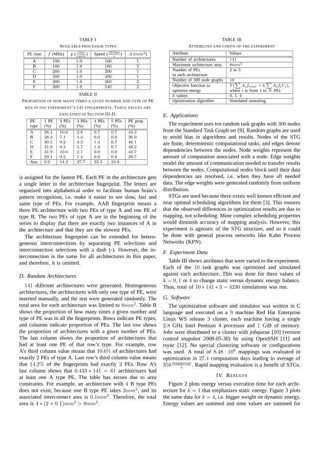
TABLE I
AVAILABLE PROCESSOR TYPES
PE type f (MHz) p ( Opscycle
) Speed (MOpss
) A (mm2)
A 100 1.0 100 1B 100 1.8 180 2C 200 1.0 200 1D 300 1.0 300 1E 200 1.8 360 2F 300 1.8 540 2
TABLE II
PROPORTION OF HOW MANY TIMES A GIVEN NUMBER AND TYPE OFPE
WAS IN THE EXPERIMENT’ S 141 FINGERPRINTS. TABLE VALUES ARE
EXPLAINED IN SECTION III-D.
PE 1 PE 2 PEs 3 PEs 4 PEs 5 PEs PE prop.type (%) (%) (%) (%) (%) (%)
A 28.4 10.6 2.8 0.7 0.7 43.3B 28.4 7.1 1.4 0.0 0.0 36.9C 30.5 9.2 4.3 1.4 0.7 46.1D 31.9 8.5 5.7 1.4 0.7 48.2E 31.9 10.6 2.1 0.0 0.0 44.7F 29.1 9.2 1.4 0.0 0.0 39.7Any 0.0 14.2 27.7 33.3 24.8
is assigned for the fastest PE. Each PE in the architecture getsa single letter in the architecture fingerprint. The lettersareorganized into alphabetical order to facilitate human brain’spattern recognition, i.e. make it easier to see slow, fast andsame type of PEs. For example, AAB fingerprint means athree PE architecture with two PEs of type A and one PE oftype B. The two PEs of type A are in the beginning of theseries to display that there are exactly two instances of A inthe architecture and that they are the slowest PEs.
The architecture fingerprint can be extended for hetero-geneous interconnections by separating PE selections andinterconnection selections with a dash (-). However, the in-terconnection is the same for all architectures in this paper,and therefore, it is omitted.
D. Random Architectures
141 different architectures were generated. Homogeneousarchitectures, the architectures with only one type of PE, wereinserted manually, and the rest were generated randomly. Thetotal area for each architecture was limited to8mm2. Table IIshows the proportion of how many times a given number andtype of PE was in all the fingerprints. Rows indicate PE types,and columns indicate proportion of PEs. The last row showsthe proportion of architectures with a given number of PEs.The last column shows the proportion of architectures thathad at least one PE of that row’s type. For example, rowA’s third column value means that10.6% of architectures hadexactly2 PEs of type A. Last row’s third column value meansthat 14.2% of the fingerprints had exactly2 PEs. Row A’slast column shows that0.433 ∗ 141 = 61 architectures hadat least one A type PE. The table has zeroes due to areaconstraints. For example, an architecture with4 B type PEsdoes not exist, because one B type PE takes2mm2, and itsassociated interconnect area is0.1mm2. Therefore, the totalarea is4 ∗ (2 + 0.1)mm2 > 8mm2.
TABLE III
ATTRIBUTES AND LIMITS OF THE EXPERIMENT
Attribute Values
Number of architectures 141Maximum architecture area 8mm2
Number of PEs 2 to 5in each architectureNumber of 300 node graphs 10
Objective function to T (∑
Aifmax + k∑
AifiUi),optimize energy wherei is from 1 to N PEsk values 0, 1, 4Optimization algorithm Simulated annealing
E. Applications
The experiment uses ten random task graphs with300 nodesfrom the Standard Task Graph set [9]. Random graphs are usedto avoid bias in algorithms and results. Nodes of the STGare finite, deterministic computational tasks, and edges denotedependencies between the nodes. Node weights represent theamount of computation associated with a node. Edge weightsmodel the amount of communication needed to transfer resultsbetween the nodes. Computational nodes block until their datadependencies are resolved, i.e. when they have all neededdata. The edge weights were generated randomly from uniformdistribution.
STGs are used because there exists well known efficient andnear optimal scheduling algorithms for them [3]. This ensuresthat the observed differences in optimization results are due tomapping, not scheduling. More complex scheduling propertieswould diminish accuracy of mapping analysis. However, thisexperiment is agnostic of the STG structure, and so it couldbe done with general process networks like Kahn ProcessNetworks (KPN).
F. Experiment Data
Table III shows attributes that were varied in the experiment.Each of the10 task graphs was optimized and simulatedagainst each architecture. This was done for three values ofk = 0, 1 or 4 to change static versus dynamic energy balance.Thus, total of10 ∗ 141 ∗ 3 = 4230 simulations was run.
G. Software
The optimization software and simulator was written in Clanguage and executed on a9 machine Red Hat EnterpriseLinux WS release 3 cluster, each machine having a single2.8 GHz Intel Pentium 4 processor and1 GiB of memory.Jobs were distributed to a cluster withjobqueue[10] (versioncontrol snapshot2008-05-30) by using OpenSSH [11] andrsync [12]. No special clustering software or configurationswas used. A total of8.48 · 108 mappings was evaluated inoptimization in27.4 computation days leading to average of358mappings
s . Rapid mapping evaluation is a benefit of STGs.
IV. RESULTS
Figure 2 plots energy versus execution time for each archi-tecture fork = 1 that emphasizes static energy. Figure 3 plotsthe same data fork = 4, i.e. bigger weight on dynamic energy.Energy values are summed and time values are summed for

0 0.5 1 1.5 2 2.5 30
0.5
1
1.5
2
2.5
3x 10
−3
Relative energy E (1)
Exe
cutio
n tim
e T
(s)
2 PEs, k = 13 PEs, k = 14 PEs, k = 15 PEs, k = 1
Fig. 2. Energy-time plot for different architectures withk = 1
0 1 2 3 4 5 60
0.5
1
1.5
2
2.5
3x 10
−3
Relative energy E (1)
Exe
cutio
n tim
e T
(s)
2 PEs, k = 43 PEs, k = 44 PEs, k = 45 PEs, k = 4
Fig. 3. Energy-time plot for different architectures withk = 4
each application. EnergyE is the sum of objective functionvalues (1) for a given architecture. Execution timeT is the sumof execution times for a given architecture. Time is measuredin seconds. Time is comparable even between differentkvalues, but energy is not. A pair(E, T ) presents a data point,or architecture, in the figure.E varied in range[1.7, 3.1] fork = 1, and [4.0, 5.8] for k = 4. Execution time sumT variedin range[0.43, 3.85]ms for both cases.
Pareto optimal solution boundary is marked with straightlines. These are not absolute Pareto optimums as not all possi-ble architectures were evaluated. A Pareto optimal architectureis such that improving either energy or execution time leadsto worsening the other factor. That is, in the Pareto optimalarchitectures, there are no two architectures where the otheris better in terms of both energy and execution time.
TABLE IV
TOP10 ARCHITECTURES TOGETHER WITH3 PARETO OPTIMAL
ARCHITECTURES FORk = 0. ARCHITECTURES ARE LABELED WITH
RESPECT TO THEIR ARCHITECTURE FINGERPRINTS. PARETO OPTIMAL
ARCHITECTURES ARE MARKED WITH*. B EST VALUES IN EACH COLUMN
ARE IN BOLD.
Arch. E T EAAE
TAAT
UP UI Afinger- (1) (ms) (1) (1) (%) (%) (mm2)
CC* 0.925 1.926 1.999 1.999 100 10 2.4DD* 0.925 1.285 1.999 2.998 100 14 2.4CCC 0.928 1.289 1.993 2.989 100 28 3.6DDD* 0.928 0.860 1.991 4.481 99 41 3.6CCE 0.935 1.016 1.977 3.789 99 35 4.6CE 0.935 1.375 1.977 2.800 100 13 3.4DF 0.936 0.917 1.976 4.199 100 20 3.4DDF* 0.936 0.678 1.975 5.677 99 51 4.6CCCC 0.941 0.980 1.965 3.931 98 52 4.8CEE 0.941 0.840 1.964 4.583 99 42 5.6DFF* 0.943 0.561 1.961 6.864 99 62 5.6FFF* 0.953 0.482 1.939 7.999 98 73 6.6DFFF* 1.001 0.428 1.847 9.005 90 96 7.8
A. Top Architectures
Table IV, Table V and Table VI show top10 and allPareto optimal architectures for casesk = 0, k = 1 andk = 4, respectively.k = 0 case is practically pure performanceoptimization, although measured in energy, butk = 1 andk = 4 are strictly energy optimization. EnergyE and totalexecution timeT are absolute values, and they are comparableto the slowest2-PE architecture AA.EAA
E is the energy gainover AA architecture, the bigger the better.TAA
T is the speedupover AA architecture, the bigger the better.UP is the meanPE utilization.UI is the mean interconnect utilization.A isthe area measured in square millimeters.
CC wins energy with all values ofk. In k = 1 case, it is1.7% more energy-efficient than the nearest3 PE solution,CCC. It is 4, 5% more energy-efficient than the nearest4PE solution, CCCC. When the role of the dynamic energyincreases ink = 4, the differences are larger:2.5% and6.2%against CCC and CCCC, respectively.
DFFF is the fastest architecture, and also a Pareto optimum.It has the highest performance processors given the areaconstraints. Note that5 PE solutions do not have performanceadvantage over4 PE solutions due to area constraints. For allvalues ofk, DFFF runs at4.5× speed compared to the mostenergy-efficient architecture CC. However, it consumes only8.2% (k = 0) to 14.3% (k = 4) more energy.
Most energy-efficient architectures have lower interconnectutilization UI and higher processor utilizationUP than thefastest architectures. Lower processor utilization in high per-formance architectures can be explained with high peeks ofperformance demand that they can satisfy. Low performancearchitectures have longer task queues during peeks, whichbalances the load in time, but makes the critical path longer.
Approximately half the architectures are homogeneous intop 10.
Table VII and Table VIII show the proportion of how manytimes a given number and type of PE was in top10 least

TABLE V
TOP10 ARCHITECTURES TOGETHER WITH3 PARETO OPTIMAL
ARCHITECTURES FORk = 1. FIGURE 2 SHOWS ARCHITECTURES
GENERATED FORk = 1 CASE.
Arch. E T EAAE
TAAT
UP UI Afinger- (1) (ms) (1) (1) (%) (%) (mm2)
CC* 1.707 1.926 1.541 1.999 100 10 2.4DD* 1.708 1.285 1.541 2.998 100 14 2.4CCC 1.736 1.289 1.516 2.988 99 27 3.6DDD* 1.737 0.860 1.515 4.479 99 40 3.6CE 1.773 1.376 1.484 2.800 100 13 3.4DF 1.773 0.917 1.484 4.199 100 19 3.4CCE 1.783 1.016 1.476 3.791 100 34 4.6CCCC 1.784 0.980 1.475 3.929 98 50 4.8DDF* 1.784 0.678 1.475 5.679 99 51 4.6DDDD* 1.798 0.663 1.464 5.810 96 73 4.8DFF* 1.817 0.561 1.448 6.864 99 61 5.6FFF* 1.847 0.482 1.425 7.998 98 72 6.6DFFF* 1.907 0.427 1.380 9.028 90 95 7.8
TABLE VI
TOP10 ARCHITECTURES TOGETHER WITH3 PARETO OPTIMAL
ARCHITECTURES FORk = 4. FIGURE 3 SHOWS ARCHITECTURES
GENERATED FORk = 4 CASE.
Arch. E T EAAE
TAAT
UP UI Afinger- (1) (ms) (1) (1) (%) (%) (mm2)
CC* 4.055 1.927 1.228 1.999 100 9 2.4DD* 4.056 1.285 1.228 2.998 100 14 2.4CCC 4.158 1.290 1.198 2.986 99 26 3.6DDD* 4.159 0.861 1.197 4.476 99 40 3.6CD 4.239 1.541 1.175 2.500 100 12 2.4CE 4.285 1.376 1.162 2.800 100 13 3.4DF 4.285 0.917 1.162 4.199 100 19 3.4CCCC 4.308 0.980 1.156 3.930 98 49 4.8DDDD* 4.319 0.663 1.153 5.812 96 71 4.8CCE 4.325 1.018 1.151 3.785 99 33 4.6DFF* 4.438 0.561 1.122 6.862 99 60 5.6FFF* 4.526 0.482 1.100 7.990 98 70 6.6DFFF* 4.633 0.430 1.075 8.952 91 93 7.8
energy consuming architectures for casesk = 1 andk = 4.In k = 1 andk = 4 cases,2 PE solutions filled4 and5 of
the top10 positions, respectively.3 PE solutions filled4 and3in those cases.4 PE solutions filled2 positions in both cases.2and3 PE solutions seem suitable for low energy applications.However,3 and4 PE solutions have high performance.
There are no A and B type PEs in the top10. This can beattributed to poor performance and energy inefficiency.fmax
is a determining factor for static energy (1), and it puts pro-cessors with frequency less thanfmax into disadvantage. Theminimum value offmax is 200MHz, because the interconnectis clocked at200MHz. For this reason, A and B types arenot favored. However, C and E types have the advantage ofnot increasingfmax. C type was the most common processoramong low-energy architectures.
B. Pareto Optimal Solutions
Pareto optimal solutions are labeled with asterisk (*) inTable V and Table VI.
For the k = 1 case, static energy proportion for Paretooptimal architectures varies between52% and 54%. For the
TABLE VII
PROPORTION OF HOW MANY TIMES A GIVEN NUMBER AND TYPE OFPE
WAS IN TOP 10 ARCHITECTURES WITHk = 1. TABLE VALUES ARE
EXPLAINED IN SECTION III-D.
PE Once Twice 3 times 4 times PEtype (%) (%) (%) (%) prop.
A 0 0 0 0 0B 0 0 0 0 0C 10 20 20 10 60D 10 20 20 10 60E 20 0 0 0 20F 20 0 0 0 20
TABLE VIII
PROPORTION OF HOW MANY TIMES A GIVEN NUMBER AND TYPE OFPE
WAS IN TOP 10 ARCHITECTURES WITHk = 4. TABLE VALUES ARE
EXPLAINED IN SECTION III-D.
PE Once Twice 3 times 4 times PEtype (%) (%) (%) (%) prop.
A 0 0 0 0 0B 0 0 0 0 0C 20 20 10 10 60D 20 10 10 10 50E 20 0 0 0 20F 10 0 0 0 10
k = 4 case, it varies between between21% and 23%. Thus,the energy profile is rather uniform for both cases.
Pareto optimal solutions have2, 3 and4 PEs.2-PE solutionsdo well due to low energy.3 and 4 PE systems are do welldue to a trade-off between energy and performance.
Figure 2 and Figure 3 show the clustering of solutions in thedesign space. Pareto optimal solutions constitute mere5% and6% of all solutions (7 and8 out of 141) for k = 1 andk = 4,respectively. Therefore, automatic exploration is neededevenwhen design space is limited to only6 types of PEs and2to 5 PEs per architecture. It is not feasible to try out thesesolutions by manual work.
C. Optimization Convergence
Figure 4 and Figure 5 plot ratioEAA
E against mappingiterations for each Pareto optimal solution. The number ofiterations it takes to win AA increases as the number ofPEs increases. This comes from increased complexity of themapping problem and the SA mapping algorithm that scales upiterations with respect to architecture complexity, the numberof PEs.4 PE architectures take over20000 more iterationsthan 3 PE architectures to reach the level of AA (the gainvalue1.0).
Our earlier work [8] presented an automated parameteri-zation method for SA mapping. Originally it was only usedfor homogeneous architectures and performance optimization.The energy-time trade-offs presented in this paper indicate thatthe method can also be used for heterogeneous architecturesand energy optimization.
In order to reach energy-efficiency of even AA architecture,it takes tens of thousands of mappings for4 PE systems.Hence, it is a non-trivial problem in most cases. This cre-ates demand for automated mapping (exploration). This mayrequire behavior level simulation due to simulation time,

0 2 4 6 8 10 12 14 16 18
x 104
1
1.1
1.2
1.3
1.4
1.5
1.6
1.7
1.8
1.9
2
Mapping iterations
Ave
rage
ene
rgy
gain
CC, k = 1DD, k = 1DDD, k = 1DDF, k = 1DFF, k = 1FFF, k = 1DDDD, k = 1DFFF, k = 1
CC, DD
DDD DDF
DFF
FFF DDDD
DFFF
Fig. 4. Average energy gain plotted against mapping optimization iterationsfor thek = 1 case. Gain is computed as reference energy value divided by anenergy value. Average gain is normalized to the average best objective valueof the AA architecture. DD architecture’s value1.7 means AA consumed1.7 times the energy of DD.
0 2 4 6 8 10 12 14 16 18
x 104
1
1.1
1.2
1.3
1.4
1.5
1.6
1.7
1.8
1.9
2
Mapping iterations
Ave
rage
ene
rgy
gain
CC, k = 4DD, k = 4DDD, k = 4DFF, k = 4FFF, k = 4DDDD, k = 4DFFF, k = 4
CC, DDDDD
FFFDFF
DDDD
DFFF
Fig. 5. Average energy gain plotted against mapping optimization iterationsfor the k = 4 case.
as was done in this paper. More accurate simulation mayneed thousands of CPUs. Fortunately, thousands of CPUs arereachable with current development budgets.
V. CONCLUSION
We evaluated heterogeneous architectures by optimizingboth energy and performance for applications. The energy ver-sus performance trade-off was analyzed by looking at Paretooptimal solutions. It was found that both energy-efficient andwell performing solutions exist, and in general, performance istraded for energy-efficiency. Results indicated that automatedexploration tools are needed when the mapping problemcomplexity grows, starting already with our experiment setup:6 types of PEs to select from, and the system consists of2 to
5 PEs.Also, the results show that our Simulated Annealing method
can be used in energy optimization for heterogeneous architec-tures, as well as in performance optimization for homogeneousarchitectures.
In the future, we plan to utilize SA to directly seek anoptimal HW allocation and consider the bus or NoC energymore closely.
REFERENCES
[1] M. Gries, Methods for evaluating and covering the design space duringearly design development, Integration, the VLSI Journal, Vol. 38, Issue 2,pp. 131-183, 2004.
[2] W. Wolf, The future of multiprocessor systems-on-chips, Design Au-tomation Conference 2004, Proceedings. 41st, pp. 681-685, 2004.
[3] Y.-K. Kwok and I. Ahmad,Static scheduling algorithms for allocatingdirected task graphs to multiprocessors, ACM Comput. Surv., Vol. 31,No. 4, pp. 406-471, 1999.
[4] H. Orsila, E. Salminen, M. Hannikainen, T.D. Hamalainen, OptimalSubset Mapping And Convergence Evaluation of Mapping Algorithmsfor Distributing Task Graphs on Multiprocessor SoC, InternationalSymposium on System-on-Chip, 2007.
[5] S. Kirkpatrick, C. D. Gelatt Jr., M. P. Vecchi,Optimization by simulatedannealing, Science, Vol. 200, No. 4598, pp. 671-680, 1983.
[6] T. Kangas, P. Kukkala, H. Orsila, E. Salminen, M. Hannikainen,T.D. Hamalainen, J. Riihimaki, K. Kuusilinna, UML-based Multi-Processor SoC Design Framework, Transactions on Embedded Com-puting Systems, ACM, 2006.
[7] G. Kahn,The semantics of a simple language for parallel programming,Information Processing, pp. 471-475, 1974.
[8] H. Orsila, T. Kangas, E. Salminen, T. D. Hamalainen,ParameterizingSimulated Annealing for Distributing Task Graphs on multiprocessorSoCs, International Symposium on System-on-Chip, 2006, pp. 73-76.
[9] Standard task graph set, ONLINE:http://www.kasahara.elec.waseda.ac.jp/schedule, 2003.
[10] jobqueue. Software. ONLINE:http://zakalwe.fi/ shd/foss/jobqueue/[11] OpenSSH, software, ONLINE:http://openssh.org[12] rsync, software, ONLINE:http://rsync.samba.org

146 Publication 5

PUBLICATION 6
H. Orsila, E. Salminen, T. D. Hamalainen, Best Practices for Simulated Annealing inMultiprocessor Task Distribution Problems, Chapter 16 of the Book “Simulated An-nealing”, ISBN 978-953-7619-07-7, I-Tech Education and Publishing KG, pp. 321-342, 2008.
Copyright 2008 Tampere University of Technology. Reproduced with permission.

16
Best Practices for Simulated Annealing in Multiprocessor Task Distribution Problems
Heikki Orsila, Erno Salminen and Timo D. Hämäläinen Department of Computer Systems Tampere University of Technology
P.O. Box 553, 33101 Tampere, Finland
1. Introduction
Simulated Annealing (SA) is a widely used meta-algorithm for complex optimization problems. This chapter presents methods to distribute executable tasks onto a set of processors. This process is called task mapping. The most common goal is to decrease execution time via parallel computation. However, the presented mapping methods are not limited to optimizing application execution time because the cost function is arbitrary. The cost function is also called an objective function in many works. A smaller cost function value means a better solution. It may consider multiple metrics, such as execution time, communication time, memory, energy consumption and silicon area constraints. Especially in embedded systems, these other metrics are often as important as execution time. A multiprocessor system requires exploration to find an optimized architecture as well as the proper task distribution for the application. Resulting very large design space must be pruned systematically with fast algorithms, since the exploration of the whole design space is not feasible. Iterative algorithms evaluate a number of application mappings for each architecture, and the best architecture and mapping is selected in the process. The optimization process is shown in Figure 1(a). The application, the HW platform and an initial solution are fed to a mapping component. The mapping component generates a new solution that is passed to a simulation component. The simulation component determines relevant metrics of the solution. The metrics are passed to a cost function which will evaluate the badness (cost) of the solution. The cost value is passed back to the mapping component. The mapping component will finally terminate the optimization process and output a final solution. The system that is optimized is shown in Figure 1(b). The system consists of the application and the HW platform. The application consists of tasks which are mapped to processing elements (PEs). The PEs are interconnected with a communication network. The chapter has two focuses: � optimize the cost function and � minimize the time needed for simulated annealing. First, the task distribution problem is an NP problem which implies that a heuristic algorithm is needed. The focus is on reaching as good as possible mapping. Unfortunately the true optimum value is unknown for most applications, and therefore the relative

Simulated Annealing
322
goodness of the solution to the true optimum is unknown. Experiments rely on convergence rates and extensive simulations to reduce this uncertainty. This chapter focuses on single-objective rather than multi-objective optimization.
Figure 1(a). Optimization process. Boxes indicate data. Ellipses indicate operations. This chapter focuses on the mapping part.
Figure 1(b). The system that is optimized. The system consists of the application and the HW platform. PE is processing element.
Second, the focus is minimizing the optimization time. A valid solution must be found in a reasonable time which depends on the application and the target multiprocessor platform. This chapter is structured as follows. We first introduce the problem of mapping a set of tasks onto a multiprocessor system. Then, we present a generic SA algorithm and give detailed analysis how the major functions may be implemented. That is followed by an overview of reported case studies, including our own. Last we discuss the findings and present the most important open research problems.

Best Practices for Simulated Annealing in Multiprocessor Task Distribution Problems
323
2. Task mapping problem
The application in Figure 1(b) is divided into tasks. Tasks are defined as smallest components in the application that can be relocated to any or some PEs in the HW platform. A mapping algorithm will find a location for each task on some PE. The application model is irrelevant for the general mapping problem as long as the application model has mappable tasks. Mapping can be done on run-time or design-time. There are several types of application models that are used in literature: directed acyclic task graphs (Kwok & Ahmad, 1999), Kahn Process Networks (Wikipedia, 2008b) and others. The mapping affects several properties of the system. Affected hardware properties are processor utilization, communication network utilization and power. Affected software and/or hardware properties are execution time, memory usage, and application and hardware context switches.
2.1 Application model Tasks can be dependent on each other. Task A depends on task B if task A needs data or control from task B. Otherwise tasks are independent. There are application models with dependent and independent tasks. Models with independent tasks are easier to map because there is zero communication between tasks. This enables the problem to be solved in separate sub-problems. However, independent tasks may affect each other if they compete for shared resources, such as a PE or a communication network. Scheduling properties of the application model may complicate evaluating a mapping algorithm.
2.2 Hardware platform model The HW platform in Figure 1(b) can be heterogeneous which means that it executes different tasks with different characteristics. These characteristics include speed and power, for example. This does not complicate the mapping problem, but affects the simulation part in Figure 1(a). The mapping problem is the same regardless of the simulation accuracy, but the mapping solution is affected. This enables both fast and slow simulation models to be used with varying accuracy. Inaccurate models are usually based on estimation techniques. Accurate models are based on hardware simulation or native execution of the system that is being optimized. Accurate models are usually much slower than inaccurate models and they may not be available at the early phase of the system design. Depending on the application model, all PEs can not necessarily execute all tasks. Restricting mappability of tasks makes the optimization problem easier and enables shortcut heuristics to be used in optimization. The previous definition for tasks excludes application components that can not be relocated, and therefore each task has at least 2 PEs where it can be executed.
2.3 Limiting the scope of problems We assume that communicating between two processors is much more expensive than communicating within a single processor. To generalize this idea, it is practically happening inside single processor computer systems because registers can be 100 times as fast as physical memory, and cache memory is 10 times as fast as physical memory. Multiprocessor systems could spend thousands of cycles to pass a message from one processor to other.

Simulated Annealing
324
This trend is constantly changing as multicore and non-asymmetric computer architectures are becoming more common. We also assume that distributed applications are not embarrassingly parallel (Wikipedia, 2008a). Without previous two assumptions the optimization algorithms can be trivially replaced with on-demand best-effort distributed job queues. This paper only considers the single-objective optimization case. Single-objective optimization finds the minimum for a given objective function. Multi-objective optimization tries to minimize several functions, and the result is a set of trade-offs, or so called Pareto-optimal solutions. Each trade-off solution minimizes some of the objective functions, but not all. Having a systematic method for selecting a single solution from the trade-off set reduces the problem into a single-objective optimization task.
2.4 Random mapping algorithm Random mapping algorithm is a simple Monte Carlo algorithm that randomizes processor assignment of each task at every iteration. The Monte Carlo process converges very slowly as it does not have negative feedback for moves into worse mappings. Random mapping algorithm is important because it sets the reference for minimum efficiency of any mapping algorithm. Any mapping algorithm should be able to do better than random mapping. Simulated Annealing algorithm produces a "Monte Carlo -like" effect at very high temperatures as almost all worsening moves are accepted.
3. Simulated annealing
Simulated Annealing is a probabilistic non-greedy algorithm (Kirkpatrick et al., 1983) that explores the search space of a problem by annealing from a high to a low temperature. Probabilistic behavior means that SA can find solutions of different goodness between independent runs. Non-greedy means that SA may accept a move into a worse state, and this allows escaping local minima. The algorithm always accepts a move into a better state. Move to a worse state is accepted with a changing probability. This probability decreases along with the temperature, and thus the algorithm starts as a non-greedy algorithm and gradually becomes more and more greedy. This chapter focuses only on using SA for mapping. The challenge is to find efficient optimization parameters for SA. (Braun et al., 2001) is a comparison of different mapping algorithms, such as Tabu Search, Genetic Algorithms, Load Balancing algorithms and others. Figure 2 shows an example of SA optimization process. Optimization begins from a high temperature where the accepted cost changes chaotically. As the temperature decreases the accepted cost changes less chaotically and the algorithm becomes greedier. Figure 3 shows the general form of Simulated Annealing algorithm pseudo-code. Table 1 shows symbols, functions and various parameters for the pseudo-code. The algorithm starts with an initial solution 0S (state). SA iterates through solutions until a termination
condition is reached. At each temperature level, SA moves one or several tasks to different PEs and evaluates the cost of the new mapping solution. Then SA either accepts or rejects the new solution. If the new solution is accepted, it is used as a basis for the next iteration. Otherwise, the new solution is thrown away.

Best Practices for Simulated Annealing in Multiprocessor Task Distribution Problems
325
0 2000 4000 6000 8000 10000 12000 14000 160000.88
0.9
0.92
0.94
0.96
0.98
1
Mapping iteration
Norm
alize
d cos
t
Accepted costBest cost
Figure 2. Cost per iteration plotted for Simulated Annealing when mapping a 100 task application to a 4 processor system. The cost is normalized so that initial cost 0 1.0C � . The plot is average filtered with a 256 sample window to hide the chaotic nature of the random process. This is also the reason why accepted cost does not always seem to touch the best cost line.
Simulated Annealing(S0)1 S ← S0
2 C ← Cost(S0)3 Sbest ← S4 Cbest ← C5 R ← 06 for i← 0 to ∞7 do T ← Temp(i)8 Snew ←Move(S, T )9 Cnew ← Cost(Snew)
10 ΔC ← Cnew − C11 if ΔC < 0 or Accept(ΔC, T )12 then if Cnew < Cbest
13 then Sbest ← Snew
14 Cbest ← Cnew
15 S ← Snew
16 C ← Cnew
17 R ← 018 else R ← R + 119 if Terminate(i, R) = True
20 then break
21 return Sbest
Figure 3. Pseudo-code of the Simulated Annealing algorithm. See Table 1 for explanation of symbols.
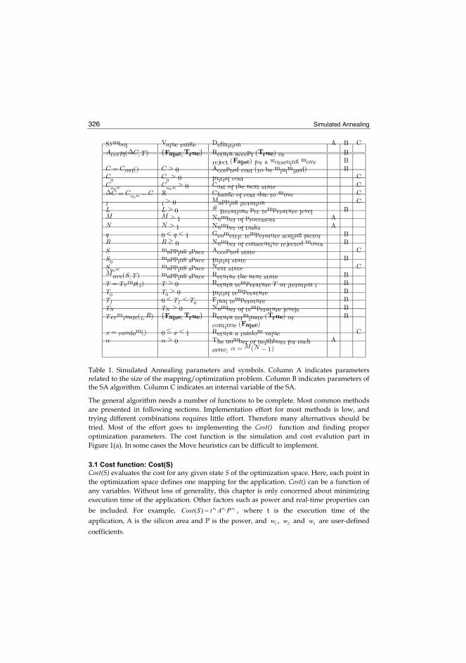
Simulated Annealing
326
Symbol Value range Definition A B C
Accept(ΔC, T ) {False,True} Return accept (True) or Breject (False) for a worsening move B
C = Cost() C > 0 Accepted cost (to be minimized) BC0 C0 > 0 Initial cost CCnew Cnew > 0 Cost of the next state CΔC = Cnew − C R Change of cost due to move Ci i > 0 Mapping iteration CL L > 0 # Iterations per temperature level BM M > 1 Number of processors AN N > 1 Number of tasks Aq 0 < q < 1 Geometric temperature scaling factor BR R ≥ 0 Number of consecutive rejected moves BS mapping space Accepted state CS0 mapping space Initial state BSnew mapping space Next state CMove(S, T ) mapping space Returns the next state BT = Temp(i) T > 0 Return temperature T at iteration i BT0 T0 > 0 Initial temperature BTf 0 < Tf < T0 Final temperature BTN TN > 0 Number of temperature levels BTerminate(i, R) {False,True} Return terminate (True) or B
continue (False)x = random() 0 ≤ x < 1 Return a random value Cα α > 0 The number of neighbors for each A
state: α = M(N − 1)
Table 1. Simulated Annealing parameters and symbols. Column A indicates parameters related to the size of the mapping/optimization problem. Column B indicates parameters of the SA algorithm. Column C indicates an internal variable of the SA.
The general algorithm needs a number of functions to be complete. Most common methods are presented in following sections. Implementation effort for most methods is low, and trying different combinations requires little effort. Therefore many alternatives should be tried. Most of the effort goes to implementing the Cost() function and finding proper optimization parameters. The cost function is the simulation and cost evalution part in Figure 1(a). In some cases the Move heuristics can be difficult to implement.
3.1 Cost function: Cost(S) Cost(S) evaluates the cost for any given state S of the optimization space. Here, each point in the optimization space defines one mapping for the application. Cost() can be a function of any variables. Without loss of generality, this chapter is only concerned about minimizing execution time of the application. Other factors such as power and real-time properties can
be included. For example, 31 2( ) ww wCost S t A P� , where t is the execution time of the
application, A is the silicon area and P is the power, and 1w , 2w and 3w are user-defined
coefficients.

Best Practices for Simulated Annealing in Multiprocessor Task Distribution Problems
327
3.2 Annealing schedule: Temp(i) function Temp(i) determines the temperature as a function of the iteration number i. Initial temperature 0 (0)T Temp� . The final temperature fT is determined implicitly by Temp() and
Terminate() functions. Temp() function may also contain internal state, and have access to other annealing metrics, such as cost. In those cases Temp() is not a pure function. For example, remembering cost history can be used for intelligent annealing schedules. In geometric temperature schedules the temperature is multiplied by a factor 0 1q� � between each temperature level. It is the most common approach. NT is the number of temperature levels. Define L to be the number of iterations on each temperature level. There are 3 common schedules that are defined in following paragraphs. Geometric Temperature Schedule
0( )i
LTemp i T q� �� �� �� (1)
i
L� �� �� �
means rounding down the fraction. The number of mapping iterations is NLT .
Fractional Temperature Schedule
0( )1
TTemp i
i�
� (2)
The number of mapping iterations is NT . It is inadvisable to use a fractional schedule because it distributes the number of iterations mostly to lower temperatures. Doubling the total number of iterations only halves the final temperature. Therefore, covering a wide
relative temperature range 0 1f
T
T�� is expensive. The geometric schedule avoids this
problem. For this reason the geometric temperature schedule is the most common choice. Koch Temperature Schedule
,
0
( 1)if mod( , ) 0
( 1)1
( ) ( 1) if mod( , ) 0
if 0
i L i
Temp ii L
Temp i
Temp i Temp i i L
T i
�� �
�� �� ���
��� � ��� �����
(3)
where
, { ( ) | }i L i kstddev Cost S i L k i� � � � � � (4)
Koch temperature schedule (Koch, 1995; Ravindran, 2007) decreases temperature with respect to cost standard deviation on each temperature level. Deviation is calculated from the L latest iterations. Higher standard deviation, i.e. more chaotic the annealing, leads to lower temperature decrease between each level. The number of mapping iterations depends on the problem.
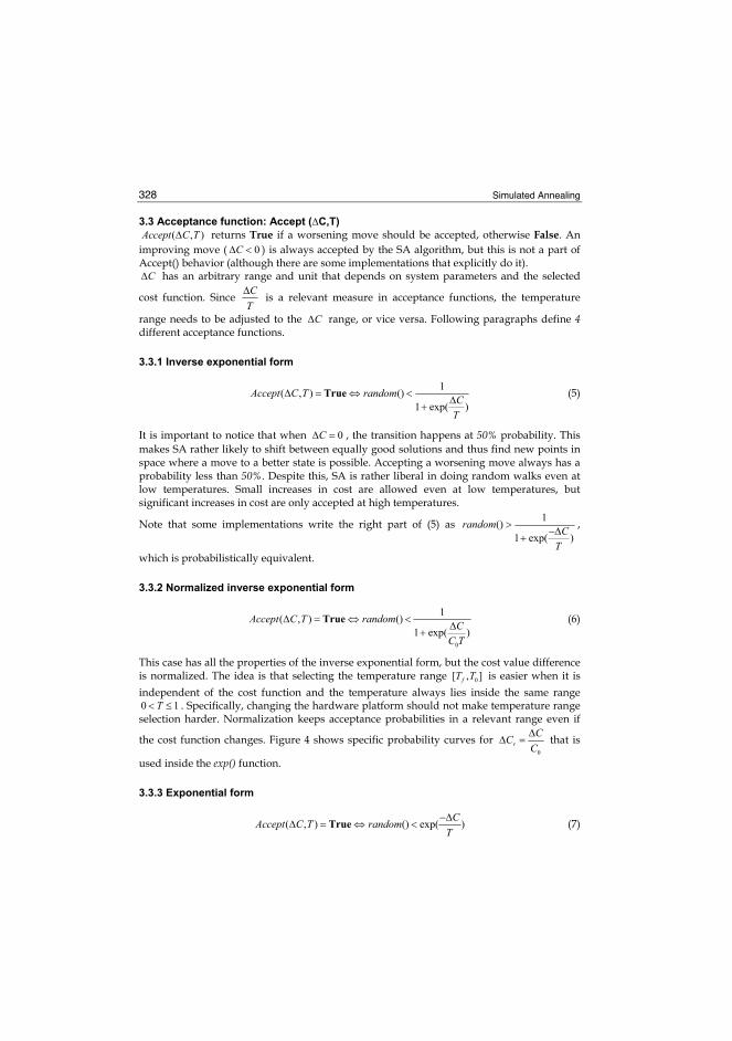
Simulated Annealing
328
3.3 Acceptance function: Accept (�C,T) ( , )Accept C T� returns True if a worsening move should be accepted, otherwise False. An
improving move ( 0C� � ) is always accepted by the SA algorithm, but this is not a part of Accept() behavior (although there are some implementations that explicitly do it). C� has an arbitrary range and unit that depends on system parameters and the selected
cost function. Since C
T
� is a relevant measure in acceptance functions, the temperature
range needs to be adjusted to the C� range, or vice versa. Following paragraphs define 4 different acceptance functions.
3.3.1 Inverse exponential form
1
( , ) ()1 exp( )
Accept C T randomC
T
� � � ��
�True (5)
It is important to notice that when 0C� � , the transition happens at 50% probability. This makes SA rather likely to shift between equally good solutions and thus find new points in space where a move to a better state is possible. Accepting a worsening move always has a probability less than 50%. Despite this, SA is rather liberal in doing random walks even at low temperatures. Small increases in cost are allowed even at low temperatures, but significant increases in cost are only accepted at high temperatures.
Note that some implementations write the right part of (5) as 1
()1 exp( )
randomC
T
���
�,
which is probabilistically equivalent.
3.3.2 Normalized inverse exponential form
0
1( , ) ()
1 exp( )Accept C T random
C
C T
� � � ��
�True (6)
This case has all the properties of the inverse exponential form, but the cost value difference is normalized. The idea is that selecting the temperature range 0[ , ]fT T is easier when it is
independent of the cost function and the temperature always lies inside the same range 0 1T� � . Specifically, changing the hardware platform should not make temperature range selection harder. Normalization keeps acceptance probabilities in a relevant range even if
the cost function changes. Figure 4 shows specific probability curves for 0
r
CC
C
�� � that is
used inside the exp() function.
3.3.3 Exponential form
( , ) () exp( )C
Accept C T randomT
��� � � �True (7)

Best Practices for Simulated Annealing in Multiprocessor Task Distribution Problems
329
Exponential form is similar to the inverse exponential form, but 0C� � transition happens always whereas the inverse exponential form accepts the same move with 50% probability. See the reasoning in inverse exponential case.
Figure 4. Acceptance probability curves for the normalized inverse exponential function (6)
with q = 0.95 . The curve represents constant values of r0
�C�C =
C. Probability of moving to
a worse state decreases when the temperature decreases. Moves to slightly worse state have higher probability than those with large degradation.
3.3.4 Normalized exponential form
0
( , ) () exp( )C
Accept C T randomC T
��� � � �True (8)
This case has all the properties of the exponential form, but in addition it is implied that temperature lies in range 0 1T� � . This is reasoned in the normalized inverse exponential case.
3.4 On effective temperature range Annealing starts with a high acceptance rate 0p for bad moves and it decreases to a very
low acceptance rate fp . It is important to control the acceptance probability. If inverse
exponential function (5) is solved with respect to T for a given probability p, we get:
1
ln( 1)
CT
p
��
� (9)

Simulated Annealing
330
Assuming minimum expected cost change minC� and maximum expected cost change
maxC� , we get the proper temperature range
min max0
0
1 1ln( 1) ln( 1)
f
f
C CT T T
p p
� �� � � �
� � (10)
Initial acceptance probability 0p should be set close to 0.5, i.e. the maximum acceptance rate for inverse exponential function, but not too close to save optimization iterations. For example, 0 0.45p � is sufficiently close to 0.5, but saves 58 temperature levels of iterations compared to 0 0.49p � , assuming 0.95q � . When 0C� � the acceptance probability is always 50%. Final acceptance probability fp can be set large enough so that a worsening move happens
n times in the final temperature level, where n is a parameter set by the designer. If there are L iterations per temperature level, we set /fp n L� . If we set 0.1n � , the final temperature
level is almost entirely greedy, and a worsening move happens with 10% probability on the temperature level for a given minC� . The temperature range becomes
min max0
0
1ln( 1) ln( 1)
f
C CT T T
L
n p
� �� � � �
� � (11)
The derivation of (10) and (11) for normalized inverse exponential, exponential and normalized exponential functions is similar.
3.5 Methods to determine the initial temperature The initial temperature 0T was not defined in annealing schedule functions in Section 3.2. As was explained in Section 3.3, the initial temperature is highly coupled with the acceptance function. Following paragraphs present common methods for computing the initial temperature. Note that final temperature is usually determined implicitly by the Terminate() function.
3.5.1 Heating The initial temperature is grown large enough so that the algorithm accepts worsening moves with some given probability 0p . This requires simulating a sufficient number of moves in the optimization space. Either moves are simulated in the neighborhood of a single point, or moves are simulated from several, possibly random, points. The average increase in cost avgC� is computed for worsening moves. Given an acceptance function, 0T is
computed such that 0 0( , )avgAccept C T p� � . The solution is trivial for all presented acceptance
functions. An example of heating is given in Section 4.2.
3.5.2 Application and hardware platform analysis Application and hardware platform analysis can be used to determine the initial temperature. Rapid methods in this category do not use simulation to initialize parameters,

Best Practices for Simulated Annealing in Multiprocessor Task Distribution Problems
331
while slow but more accurate methods use simulation. An example, see (10), (11) and Section 4.3.
3.5.3 Manual tuning Parameters can be set by manually testing different parameters. This option is discouraged for an automated optimization system where the problem varies significantly.
3.5.4 Cost change normalization In this method the temperature scale is made independent of the cost function values. This is either accomplished by (6) or setting 0 0T C� for (5). By using (6) it is easier to use other initial temperature estimation methods.
3.6 Move function and heuristics: Move(S, T ) Move(S, T) function returns a new state based on the application specific heuristics and the current state S and temperature T . Move heuristics vary significantly. The simple ones are purely random. The complex ones analyze the structure of the application and the hardware, and inspect system load. It should be noted that given a current state value, randomizing a new state value should exclude the current value, i.e. current PE of the moved task in this case, for randomization process. For example, in two-processor system, there is a 50% probability of selecting the same CPU again, which means that half of the iterations are wasted. Many papers do not specify this aspect for random heuristics. Common choices and ideas for move heuristics from literature are presented in following sections.
3.6.1 Single: move task to another processor Choose a random task and move it to a random processor.
3.6.2 Multiple: move several tasks to other processors Instead of choosing only a single task to move to another processor, several tasks can be moved at once. The moved tasks are either mapped to the same processor, or different processors. If these tasks are chosen at random and each of their destinations are chosen at random, this approach is less likely to find an improving move than just moving a single task. This is a consequence of combinatorics as improving moves are a minority group in all possible moves. If a good heuristics is applied for moving multiple tasks, it is possible to climb up from a steep local minimum. A heuristics that only moves a single task is less likely to climb up from a steep local minimum.
3.6.3 Swap: swap processes between processors Choose two different random processors, choose a random process on both processors, and swap the processes between processors.
3.7 Heuristic move functions A heuristic move uses more information than just knowing the mapping space structure. Some application or hardware specific knowledge is used to move or swap tasks more efficiently.

Simulated Annealing
332
3.7.1 ECP: Enhanced critical path Enhanced Critical Path method (Wild et al., 2003) is a heuristic move for directed acyclic task graphs. ECP favors swapping and moving processes that are on the critical path of the graph, or near the critical path. Critical path is the path with the largest sum of computation and communication costs in the graph.
3.7.2 Variable grain move A variable grain move is a single task move that starts by favoring large execution time tasks statistically. Thus, tasks with large execution time are moved more likely than tasks with small execution time. The probability distribution is then gradually flattened towards equal probability for each task. At low temperatures each task is moved with the same probability.
3.7.3 Topological move Assume tasks A and B, where A sends a message to B with a high probability after A has been activated. If B is the only task that gets a message from A with a high probability then it can be benefitial to favor moving them to the same processor. This heuristics could be implemented into Single task move by favoring processors of adjacent tasks. The probability distribution for processor selection should be carefully balanced to prevent mapping all tasks to the same processor, thus preventing speedup of a multiprocessor system. If a task sends messages to more than one task with a high probability, this heuristics is at least dubious and needs experimental verification.
3.7.4 Load balancing move This heuristics makes heavily loaded processors less likely to get new tasks, and make slightly loaded processes more likely to get new tasks. Each processor's load can be determined by a test vector simulation, by counting the number of tasks on each processor, or by using more sophisticated load calculations. Each task can be attributed a constant load based on test vector simulations, and then each processor's load becomes the sum of loads of its tasks.
3.7.5 Component move A task graph may consist from application or system level components each having multiple tasks. Separate components are defined by the designer. Instead of mapping single tasks, all tasks related to a single component could be mapped. This could be a coarse-grain starting point for finer-grain mapping.
3.8 Other move heuristics 3.8.1 Hybrid approach A hybrid algorithm might use all of the above move functions. For example, combine weighted task selection with weighted target PE selection (Sec 3.7.2 + 3.7.3). The move function can be selected by random on each iteration, or different move function can be used in different optimization phases.
3.8.2 Compositional approach SA can be combined with other algorithms. The move function may use another optimization algorithm to make more intelligent moves. For example, the single move

Best Practices for Simulated Annealing in Multiprocessor Task Distribution Problems
333
heuristics might be adapted to give more weight to the best target processor determined by actually simulating each target.
3.8.3 Optimal subset mapping move The move function can optimize a subset of the task graph. Each move will by itself determine a locally optimal mapping for some small subset of tasks. The number of mapping combinations for a subset of subN tasks and M processors is subNM for the brute-
force approach. The number of brute-combinations for a single subset should only be a tiny fraction of total number of mappings that are evaluated, that is, a large number of subsets should be optimized. A brute-force based approach may yield rapid convergence but the final result is somewhat worse than with traditional SA (Orsila et al., 2007). It is suitable for initial coarse-grain optimization.
3.8.4 Move processors from router to router In a Network-on-Chip (NoC) system, processors can be moved from router to router to optimize communication between system components.
3.8.5 Task scheduling move Scheduling of tasks can be done simultaneously with mapping them. Scheduling means determining the priorities of tasks on each processor separately. Priorities for tasks is determined by a permutation of all tasks. Task A has higher priority than task B if it is located before task B in the permutation. A permutation can be altered by swapping two random tasks in the Move function. The order of tasks is only relevant for tasks on the same processor. As an optimization for the move heuristics, most permutations need not be considered.
3.9 Termination function: Terminate(i, R) Terminate(i, R) returns True when the optimization loop should be terminated. R is the number of consecutive rejected moves, maxi is a user-defined maximum number of
iterations, and maxR is a user-defined maximum number of consecutive rejects. Terminate()
function often uses the T emp() function for determining the current temperature T. Following paragraphs present examples and analysis of commonly used termination functions from literature:
3.9.1 Maximum number of iterations Annealing is stopped after imax iterations:
max( , )Terminate i R i i� � �True (12)
This approach is discouraged because annealing success is dependent on actual temperatures, rather than iterations. Final temperature and annealing schedule parameters can be selected to restrict the maximum number of iterations.
3.9.2 Temperature threshold Annealing is stopped at a specific temperature fT :

Simulated Annealing
334
( , ) ( ) fTerminate i R Temp i T� � �True (13)
This approach is discouraged in favor of coupled temperature and rejection threshold because there can be easy greedy moves left.
3.9.3 Cost threshold Annealing is stopped when a target cost is achieved:
( , ) ( ) targetTerminate i R Cost S Cost� � �True (14)
For example, if the cost function measures real-time latency, annealing is stopped when a solution that satisfies real-time requirements is found. This heuristics should not be used alone because if the target cost is not achieved, the algorithm loops forever.
3.9.4 Rejection threshold Annealing is stopped when maxR R� :
max( , )Terminate i R R R� � �True (15)
This approach is discouraged because there is a risk of premature termination.
3.9.5 Uncoupled temperature and rejection threshold Annealing is stopped at a low enough temperature or if no improvement has occured for a while:
max( , ) ( ) fTerminate i R Temp i T R R� � � � �True (16)
This approach is discouraged because there is a risk of premature termination.
3.9.6 Coupled temperature and rejection threshold Annealing is stopped at a low enough temperature only when no improvement has occured for a while:
max( , ) ( ) fTerminate i R Temp i T R R� � � � �True (17)
This approach has the benefit of going through the whole temperature scale, and continue optimization after that if there are acceptable moves. This will probably drive the solution into a local minimum.
3.9.7 Hybrid condition Any logical combination of conditions 3.9.1 - 3.9.6 is a valid termination condition.
4. Case studies
This section summarizes 5 relevant works on the use of SA for task mapping. Task mapping problems are not identical but comparable in terms of SA parameterization. Selected SA parameterizations are presented to give insight into possible solutions. Table 2 shows move heuristics and acceptance functions, and Table 3 shows annealing schedules for the same cases. These cases are presented in detail in following sections.

Best Practices for Simulated Annealing in Multiprocessor Task Distribution Problems
335
Implementation Move Function Acceptance Function
Braun (Sec 4.1) Single Normalized Inverse ExponentialCoroyer (Sec 4.2) Single, Task Scheduling ExponentialOrsila (Sec 4.3) Single Normalized Inverse ExponentialRavindran (Sec 4.4) Single ExponentialWild (Sec 4.5) Single, ECP N/A
Table 2. Simulated Annealing move heuristics and acceptance functions
Implementation Annealing Schedule T0 End condition L
Braun (Sec 4.1) Geometric, q = 0.90 C0 Tf = 10−200 1Coroyer (Sec 4.2) Geometric, Fractional Heuristic Heuristic αOrsila (Sec 4.3) Geometric, q = 0.95 Heuristic Heuristic αRavindran (Sec 4.4) Koch T0 = 1 N/A N/AWild (Sec 4.5) Geometric, q = N/A N/A Heuristic N/A
Table 3. Simulated Annealing schedules. See Table 1 for symbols.
Single move (Sec 3.6.1) and the Geometric annealing scheduling (1) are the most common choices. They should be tested in every new experiment. All the cases use a single move so it is not covered in each case. Other choices are explicitly documented.
4.1 Braun case (Braun et al., 2001) uses an inverse exponential form (5) as an acceptance function. However, the method uses it to actually implement a normalized inverse exponential form (6) by setting 0 0T C� .
A geometric temperature schedule (1) with 0.90q � and 1L � is used. The termination condition is an uncoupled temperature and rejection threshold (16). Optimization is terminated when 20010fT
�� or when max 200R � consecutive solutions are
identical. The choice for L and fT values are not explained. If the HW platform or the
number of tasks were changed, then trivially the number of iterations should be adjusted as well. The initial mapping used was a random mapping of tasks. The paper compares SA to ten other heuristics for independent task mapping problem. SA got position 8/11, where 1/11 is the best position received by a genetic algorithm. We believe SA was used improperly in this comparison. Based on (11), we think fT was set too low,
and L should be much larger than 1.
4.2 Coroyer case (Coroyer & Liu, 1991) do both single and task scheduling (Sec 3.8.5) moves. The acceptance function is exponential (7) accompanied with a heating process that puts acceptance probabilities to a relevant range. Initial temperature is set high enough so that
0 0.95p � of new mappings are accepted. If avgC� is the average increase in cost for
generating new solutions, the initial temperature is set to 00lnavgC
Tp
��� . This approach
depends on the exponential acceptance function, but it can easily be adopted for other acceptance functions. The average increase is determined by simulating a sufficient number of moves. See Section 3.5.1.

Simulated Annealing
336
Both fractional (2) and geometric (1) temperature schedules are used with various parameters. The number of mapping iterations per temperature level is ( 1)L N M�� � � . The termination condition is an uncoupled temperature and rejection threshold (16). Optimization is terminated when 210fT
�� or when max 5R �� consecutive solutions are
identical. Also, a given temperature threshold (13) is used. The initial mapping used was a random mapping of tasks. They show that SA gives better results than priority-based heuristics for task mapping and scheduling, but SA is also much slower. Systematic methods are not used to tune parameters.
4.3 Orsila case This case presents methods to derive SA parameters systematically from the problem parameters (Orsila et al., 2006). The annealing schedule is geometric with 0.95q � . The number of iterations per temperature level is ( 1)L N M�� � � . The initial and final temperature range 0[ , ] (0,1]fT T � is defined with
max0
min sum
ktT
t� (18)
min
maxf
sum
tT
kt� (19)
where maxt and mint are the maximum and minimum execution time for any task (when it is activated) on any processor, min sumt is the sum of execution times for all tasks on the fastest processor in the system, max sumt is the sum of execution times for all tasks on the slowest processor in the system, and 1k � is a coefficient. The temperature range is tied to a slightly modified version of (6). The factor 0.5 is the only difference.
0
1( , ) ()
1 exp( )0.5
Accept C T randomC
C T
� � � ��
�True (20)
The rationale is choosing an initial temperature where the longest single task will have a fair transition probability of being moved from one processor to another, and the same should hold true for the shortest single task with respect to final temperature.
Coefficient k has an approximate relation to fp . Substituting min
00.5
C
C
� in place of minC� to
make (10) compatible with (20) gives
min
0
10.5 ln( 1)
f
f
CT T
Cp
�� �
� (21)

Best Practices for Simulated Annealing in Multiprocessor Task Distribution Problems
337
Now, min
00.5
C
C
� is approximated with min
max sum
t
t from (19)
min
max
1ln( 1)
f
sumf
tT T
tp
��
� (22)
Now comparing (19) and (22) we get the relation
1
ln( 1)f
kp
�� (23)
Solving (23) with respect to fp gives us
1
1f kp
e �� (24)
For 1k � the probability fp to accept a worsening move on the final temperature level
given a cost change of order mint is approximately 27%. For 2k � , probability is 12%. As k increases fp decreases exponentially. Suitable values for k are in range [1, 9] unless L is very
large (hundreds of thousands or even millions of iterations). The temperature range implied by 1k � is shown in Figure 5. The temperature range is calculated with (18) and (19). (Orsila et al., 2007) uses 2k � and reaches are a local minimum more likely in the end, but it is more expensive than 1k � .
Figure 5. Averaged speedup with respect to temperature for 300 node graphs with different L values. The temperature given with (18)(19) k = 1 is labeled �predicted range�. Notice that temperature and the number of iterations increase in different directions. The number of mapping iterations increases as the temperature decreases.
The end condition is the coupled temperature and rejection threshold (17) with maxR �� .
4.4 Ravindran case (Ravindran, 2007) uses an exponential acceptance function (7).

Simulated Annealing
338
A Koch temperature schedule (3) was used with parameters, including initial and final temperature, set manually. Termination condition is the temperature threshold (13). Systematic methods are not used to tune parameters. However, the Koch temperature schedule is mitigating factor since it affects the number of temperature levels and iterations based on the problem.
4.5 Wild case (Wild et al., 2003) use a geometric annealing schedule (1) with unknown parameters. The termination condition is the uncoupled temperature and rejection threshold (16). They show that an ECP move heuristics (Sec 3.7.1) is significantly better than the single move with directed acyclic graphs. Systematic methods are not used to tune parameters.
5. Analysis and discussion
Following sections analyze the effect of iterations per temperature level, saving the number of iterations, give best practices for SA, and finally, SA is compared to two greedy algorithms and random mapping.
5.1 Iterations per temperature level Figure 6 shows speedup of a 300N � task directed acyclic graph with respect to iterations
per temperature level L. Speedup is defined as 1t
t, where t is the execution time of the
optimized solution on multiprocessor system and t1 is the execution time on a single processor system.
Figure 6. Averaged speedups for 300 node graphs with M=2-8 processing elements and different L values (L = 1, 2, 4, ..., 4096) for each processing element set.
Figure 7 shows the speedup and the number of iterations for each L. These figures show that having ( 1) [300,600,900, ,2100]L N M�� � � � � for the number of processors [2,3, ,8]M � � does not yield a significant improvement in performance but optimization time is increased heavily. Parameter 1L � performs very poorly (Orsila et al., 2006).

Best Practices for Simulated Annealing in Multiprocessor Task Distribution Problems
339
Figure 7. Averaged speedup with respect to mapping evaluations for 300 node graphs with different L values.
5.2 Saving optimization effort Choosing initial temperature 0T and final temperature fT is crucial for saving optimization
iterations. With too high an initial temperature the optimization process is practically Monte Carlo which means it converges very slowly, and thus, initial iterations are practically wasted because bad moves are accepted with too high a probability. This effect is visible in Figure 5 at high temperatures, i.e. 210T �� . Also, too low a probability reduces the annealing to greedy optimization. Greedy optimization becomes useless after a short time because it can not espace local minima. Therefore the final temperature must be set as high as possible without sacrificing the greedy part in optimization. This is the rationale for (Orsila et al., 2006) in Section 4.3.
5.3 Simulated annealing best practices Based on our experiments, we have identified few rules of thumb for using SA to task mapping. 1. Choose the number of iterations per temperature level ( 1)L N M�� � � , where N is the
number of tasks and M is the number of PEs. Thus, � is the number of neighbouring mapping solutions because each of the N tasks could be relocated into at most 1M � alternatives.
2. Use geometric temperature schedule with 0.90 0.98q� � . This is the most common choice.
3. Device a systematic method for choosing the initial and final temperatures. As an example, see (10).
4. Use coupled temperature and rejection threshold as the end condition (Section 3.9.6) with maxR L� (the number of iterations per temperature level)
5. If in doubt, use the single task move (Sec 3.6.1). This is the most common choice. Other move heuristics can be very useful depending on the system. For example, ECP heuristics (Sec 3.7.1) is efficient for directed acyclic task graphs.
6. Use normalized inverse exponential function (6) as the acceptance function. This implies that temperature is always in range (0, 1]. This also means that convergence of

Simulated Annealing
340
separate annealing problems can be compared with each other, and thus, effective annealing temperatures become more apparent through experiments.
7. Optimize the same problem many times. On each optimization run start with the best known solution so far. As simulated annealing is a probabilistic algorithm it can happen that the algorithm drives itself to a bad region in the optimization space. Running the algorithm several times reduces this risk.
8. If in doubt of any of the parameters, find them experimentally 9. Record the iteration number when the best solution was reached. If the termination
iteration number is much higher than the best solution iteration, maybe the annealing can be made more efficient without sacrificing reliability.
5.4 Comparing SA to greedy algorithms Figure 8 compares SA to two greedy algorithms and Random Mapping (Orsila et al., 2007). A 300 task application is distributed onto 8 processors to optimize execution time. Group Migration (GM) is a deterministic greedy algorithm that converges slowly. GM needs many iterations to achieve any speedup, but once that occurs, the speedup increases very rapidly. Optimal Subset Mapping (OSM) is a stochastic greedy algorithm that converges very rapidly. It reaches almost the maximum speedup level with very limited number of iterations. SA convergence speed is between GM and OSM but in the end it reaches a better solution. Random mapping saturates quickly and further iterations are unable to provide any speedup. Note that SA follows the random mapping line initially as it resembles a Monte Carlo process at high temperatures. Random mapping is the base reference for any mapping algorithm since any intelligent algorithm should do better than just random.
103 104 105 1061
1.5
2
2.5
3
3.5
4
Mapping iterations (log scale)
Avera
ge ga
in (sp
eedu
p)
OSMSA+ATHybridRandomGM
RandomGM
OSM
SA+AT
Hybrid
Figure 8. SA convergence speed compared to GM, OSM and Random Mapping algorithms for mapping 300 tasks to 8 processors. SA+AT is a Simulated Annealing algorithm presented in Section 4.3. GM and OSM are greedy heuristics.
SA yields 8% better result than GM, 12% better than OSM, and 107% better than random mapping. SA is better than the greedy algorithms because it can espace local minima. However, when measuring the best speedup divided with the number of iterations needed to achieve the best result for each algorithm the relative order is different. We normalize the results so that random mapping gets value 1.00. SA gets 2.58, OSM 6.11 and GM 1.21. That

Best Practices for Simulated Annealing in Multiprocessor Task Distribution Problems
341
is, OSM is 2.4 times as efficient as SA is in terms of speedup divided by iterations. SA is 2.1 times as efficient as GM. Thus, we note that greedy local search methods can converge much faster than SA.
6. Open research challenges
This section identifies some open research challenges related to using SA for task mapping. The challenges are in order of importance. What is the optimal annealing schedule for task mapping given a hardware, application model and a trade-off between solution quality and speed? The hardware and application model determine all possible cost changes in the system, and this is tied to probabilistic SA transitions. Not all temperatures are equally useful, so iterations can be saved by not annealing on irrelevant temperatures. For example, it is not benefitial to use lots of iterations at high temperatures because the process is essentially a Monte Carlo process which converges very slowly. What are the best move heuristics for each type of application and hardware model? For example, ECP (Sec 3.7.1) is useful for application models that have the concept of critical path. What is the optimal transition probability for 0C� � ? The probability is 0.5 in (5) and 1.0 in (7), but it can be selected arbitrarily. This probability determines the tendency at which SA travels equally good solutions in the neighborhood. Is there advantage to using either (5) or (7) due to this factor? Can SA be made faster or better by first doing coarse-grain optimization on the application level and then continue with finer-grain optimization? Current optimization strategies are concerned with sequential small changes rather than employ a top-level strategy. What are the relevant test cases for comparing SA to other algorithms, or other SA implementations? (Barr et al., 1995) have laid out good rules for comparing heuristics. Excluding optimization programs, is there a problem where running SA as the main loop of the program would be benefitial? Each Cost() call would go one or several steps further in the program. In other words, is SA a feasible for run-time optimization rather than being used as an offline optimizer? Even small problems can take significant amount of iterations to get parameters correctly. The application must also tolerate slowdowns.
7. Conclusions
This chapter presents an overview of using SA for mapping application tasks to multiprocessor system. We analyze the different function variants needed in SA. Many choices are suboptimal with respect to iteration count or discouraged due to poor optimization results. We find that SA is a well performing algorithm if used properly, but in practice it is too often used badly. Hence, we present best practices for some of those and review the most relevant open research challenges. For best practices we recommend following. Iterations per temperature level should depend on the problem size. Systematic methods should be used for the temperature range. Normalized inverse exponential function should be used. For open research challenges we prioritize following. Find an optimal annealing schedule, move function and transition probabilities for each type of common task mapping problems. For example, it is possible to do critical path analysis for some task mapping problems.

Simulated Annealing
342
8. References
Barr, R. S.; Golden, B. L & Kelly, J. P. & Resende, M. G. C. & Stewart, W. R. (1995). Designing and Reporting on Computational Experiments with heuristic Methods, Springer Journal of Heuristics, Vol. 1, No. 1, pp. 9-32, 1995.
Braun, T. D.; Siegel, H. J. & Beck, N. (2001). A Comparison of Eleven Static Heuristics for Mapping a Class of Independent Tasks onto Heterogeneous Distributed Systems, IEEE Journal of Parallel and Distributed Computing, Vol. 61, pp. 810-837, 2001.
Cerny, V. (1985). Thermodynamical Approach to the Traveling Salesman Problem: An Efficient Simulation Algorithm, Journal of Opt. Theory Appl., Vol. 45, No. 1, pp. 41-51, 1985.
Coffman, E. G. Jr. & Graham, R. L. (1971). Optimal Scheduling for Two-Processor Systems, Springer Acta Informatica, Vol. 1, No. 3, pp. 200-213, September, 1971.
Coroyer, C. & Liu, Z. (1991). Effectiveness of Heuristics and Simulated Annealing for the Scheduling of Concurrent Tasks - An Empirical Comparison, Rapport de recherch´ de l'INRIA - Sophia Antipolis, No. 1379, 1991.
Kirkpatrick, S.; Gelatt, C. D. Jr. & Vecchi, M. P. (1983). Optimization by simulated annealing, Science, Vol. 200, No. 4598, pp. 671-680, 1983.
Koch, P. (1995). Strategies for Realistic and Efficient Static Scheduling of Data Independent Algorithms onto Multiple Digital Signal Processors. Technical report, The DSP Research Group, Institute for Electronic Systems, Aalborg University, Aalborg, Denmark, December 1995.
Kwok, Y.-K. & Ahmad, I. (1999). Static scheduling algorithms for allocating directed task graphs to multiprocessors, ACM Comput. Surv., Vol. 31, No. 4, pp. 406-471, 1999.
Orsila, H.; Kangas, T. & Salminen, E. & Hämäläinen, T. D. (2006). Parameterizing Simulated Annealing for Distributing Task Graphs on Multiprocessor SoCs, International Symposium on System-on-Chip 2006, Tampere, Finland, November, pp. 1-4, 2006.
Orsila, H.; Salminen, E. & Hännikäinen, M. & Hämäläinen, T. D. (2007). Optimal Subset Mapping And Convergence Evaluation of Mapping Algorithms for Distributing Task Graphs on Multiprocessor SoC, International Symposium on System-on-Chip 2007, Tampere, Finland, November, pp. 1-6, 2007.
Ravindran, K. (2007). Task Allocation and Scheduling of Concurrent Applications to Multiprocessor Systems, PhD Thesis, UCB/EECS-2007-149, [online] http://www.eecs.berkeley.edu/Pubs/TechRpts/2007/EECS-2007-149.html, 2007.
Wikipedia. (2008). Embarrassingly Parallel, [online] http://en.wikipedia.org /wiki/Embarrassingly_parallel
Wikipedia. (2008). Kahn Process Network, [online] http://en.wikipedia.org /wiki/Kahn_Process_Network
Wild, T.; Brunnbauer, W. & Foag, J. & Pazos, N. (2003). Mapping and scheduling for architecture exploration of networking SoCs, Proc. 16th Int. Conference on VLSI Design, pp. 376-381, 2003.

170 Publication 6
PUBLICATION 7
Copyright 2009 IEEE. Reprinted, with permission, from H. Orsila, E. Salminen,T. D. Hamalainen, Parameterizing Simulated Annealing for Distributing Kahn Pro-cess Networks on Multiprocessor SoCs, International Symposium on System-on-Chip, Tampere, Finland, October 2009.

Parameterizing Simulated Annealing for DistributingKahn Process Networks on Multiprocessor SoCs
Heikki Orsila, Erno Salminen and Timo D. HamalainenDepartment of Computer SystemsTampere University of Technology
P.O. Box 553, 33101 Tampere, FinlandEmail: {heikki.orsila, erno.salminen, timo.d.hamalainen}@tut.fi
Abstract—Mapping an application on Multiprocessor System-on-Chip (MPSoC) is a crucial step in architecture exploration.The problem is to minimize optimization effort and applicationexecution time. Simulated annealing (SA) is a versatile algorithmfor hard optimization problems, such as task distribution onMPSoCs. We propose an improved automatic parameter selectionmethod for SA to save optimization effort. The method deter-mines a proper annealing schedule and transition probabilitiesfor SA, which makes the algorithm scalable with respect toapplication and platform size. Applications are modeled as KahnProcess Networks (KPNs). The method was improved to optimizeKPNs and save optimization effort by doing sensitivity analysisfor processes. The method is validated by mapping 16 to 256node KPNs onto an MPSoC. We optimized 150 KPNs for 3architectures. The method saves over half the optimization timeand loses only 0.3% in performance to non-automated SA. Resultsare compared to non-automated SA, Group migration, randommapping and brute force algorithms. Global optimum solutionare obtained by brute force and compared to our heuristics.Global optimum convergence for KPNs has not been reportedbefore. We show that 35% of optimization runs reach within5% of the global optimum. In one of the selected problemsglobal optimum is reached in as many as 37% of optimizationruns. Results show large variations between KPNs generated withdifferent parameters. Cyclic graphs are found to be harder toparallelize than acyclic graphs.
I. INTRODUCTION
An efficient multiprocessor SoC (MPSoC) implementationrequires automated exploration to find an efficient HW al-location, task mapping and scheduling [1]. HeterogeneousMPSoCs are needed for low power, high performance, andhigh volume markets [2]. The central idea in MPSoCs is toincrease performance and energy-efficiency. This is achievedby efficient communication between cores and keeping clockfrequency low while providing enough parallelism.
Mapping means placing each application component tosome processing element (PE). Scheduling means determiningexecution timetable of the application components on theplatform. A large design space must be pruned systematically,since the exploration of the whole design space is not feasible[1]. Fast optimization procedure is desired in order to coverreasonable design space. However, this comes with the ex-pense of accuracy. Iterative optimization algorithms evaluatea number of application mappings for each resource allocationcandidate. The application is simulated for each mapping toevaluate the cost of a solution. The cost may depend on
multiple factors, such as execution time, energy consumptionand silicon area constraints etc. Figure I(a) shows the mappingprocess.
We present an experiment where a set of applicationsmodeled as Kahn Process Networks (KPNs) [3] are mappedon MPSoCs that have 2 to 4 PEs connected with dual sharedbus. Figure I(b) shows a conceptual view of the application,its mapping, and the hardware platform. The application isoptimized (mapped) for each architecture with respect to theapplication execution time. Resulting execution and optimiza-tion time values are compared to other mapping methods andglobal optimum solutions. Global optimum solutions are foundby brute force search for small KPNs. We have not seen asimilar comparison in any paper. It is found that KPN andarchitecture structure has a significant impact on optimization.
II. RELATED WORK
A. Kahn Process Networks (KPNs)
KPN is a distributed model of computation where a directedgraph models communicating processes that can be mappedfreely to PEs. Nodes in the graph do computation. Edges arecommunication links that are unbounded FIFOs. Each nodeexecutes a program that can read from its incoming FIFOsand write to outgoing FIFOs. There is no restriction to whatthe process may compute. Our earlier work used Static TaskGraphs (STGs) [4]. STG is a special of KPN where the graphis acyclic, and each node does only one read-compute-writecycle, in that order.
B. Algorithms For Task Mapping
Architecture exploration needs automatic tuning of opti-mization parameters for architectures of various sizes. Withoutscaling, algorithm may spend excessive time optimizing asmall system, or the solution is sub-optimal for a large system.Wild et al. [5] compared SA, Tabu Search (TS) [6] and variousother algorithms for task distribution. The parameter selectionfor SA had geometric annealing schedule that did not considerapplication or system architecture size, and thus did not scaleup to bigger problems without manual tuning of parameters.
Braun et al. [7] compared 11 optimization algorithms fortask distribution. TS outperformed SA in [5], but was worsein [7], which can be attributed to different parameter selectionused. Braun’s method has a proper initial temperature selection

Application
Mapping
HW PlatformInitial
solution
Solution
Simulation
Cost evaluat ion
(a) Optimization process. Boxes indicate data.Ellipses indicate operations.
Mapping
Application
(task graph)
PE PE PE PE
T
T
T
T
HW platform
Communication network
(b) An example MPSoC that is optimized. The system consists of theapplication and the HW platform. T denotes a task, and PE denotes aprocessing element.
Fig. 1. Diagram of the optimization process and the system that is optimized
for SA to normalize transition probabilities, but their annealingschedule does not scale up with application or system size,making both [5] and [7] unsuitable for architecture exploration.
Our earlier papers have surveyed SA for task distribu-tion [8], devised a method for automatically determiningSA parameters [9] for distributing STGs, optimized memoryconsumption in distributing STGs [10], compared SA to otheralgorithms with respect to its convergence proprties [11], andoptimized task graphs for heterogeneous architectures [12].
This paper extends and improves the method presented in[9]. The transition from STGs to KPNs requires changes tothe parameter selection method that determines an efficientannealing schedule. Also, the method is improved by doingsensitivity analysis for processes. Processes with lowest exe-cution times are ignored in the temperature range calculationto save optimization effort. Number of mapping iterationsbecomes smaller (optimization time is saved) but quality ofresults is not significantly reduced. Finally, this paper presentscomparison to brute force global optimums that does not existin earlier work. The presented method can be applied with
SIMULATED ANNEALING(S0, T0)1 S ← S0
2 C ← COST(S0)3 Sbest ← S4 Cbest ← C5 R← 06 for i← 0 to ∞7 do T ← TEMPERATURE(T0, i)8 Snew ← MOVE(S, T )9 Cnew ← COST(Snew)
10 ΔC ← Cnew − C11 if ΔC < 0 or RANDOM() < ACCEPT(ΔC, T )12 then if Cnew < Cbest
13 then Sbest ← Snew
14 Cbest ← Cnew
15 S ← Snew
16 C ← Cnew
17 R← 018 else if T ≤ Tf
19 then R← R+ 120 if R ≥ Rmax
21 then break22 return Sbest
Fig. 2. Pseudo-code of the Simulated annealing algorithm. Bolded functionsare modified for the presented parameter selection method.
general process networks, not just KPNs in this experiment.
C. Simulated Annealing
SA is a probabilistic non-greedy algorithm [13] that ex-plores search space of a problem by moving from a highto a low temperature state. At each temperature level, SAmoves one or several tasks to different PEs and evaluates thecost of new mapping solutions for each move. The algorithmalways accepts a move into a better state, but also into a worsestate with a changing probability. This probability decreasesalong with the temperature, and thus the algorithm becomesgreedier. The algorithm terminates when the final temperatureis reached and sufficient number of consecutive moves havebeen rejected.
Fig. 2 shows the pseudo-code of the SA algorithm used withthe new method for parameter selection. Implementation spe-cific issues compared to the original algorithm are explainedin Section III. The Cost function evaluates execution time ofa specific mapping by calling the scheduler. S0 is the initialmapping of the system, T0 is the initial temperature, andS and T are current mapping and temperature, respectively.Temperature function computes a new temperature as afunction of initial temperature T0 and iteration i. R is the num-ber of consecutive rejects. Move function moves a randomtask to a random PE, different than the original PE. Randomfunction returns an uniform random value from the interval[0, 1). Accept function computes a probability for acceptinga move that increases the cost. Rmax is the maximum numberof consecutive rejections allowed after the final temperaturehas been reached.

III. THE PARAMETER SELECTION METHOD FOR KPNS
The parameter selection method defines Temperature andAccept functions for the pseudo-code presented in Figure 2.This creates an efficient annealing schedule with effective tran-sition probabilities. We call this method Simulated annealingwith automatic temperature (SA+AT).
A. Temperature Function
Temperature function is chosen so that annealing schedulelength is proportional to application and system architecturesize. Moreover the initial temperature T0 and final temper-ature Tf must be in the relevant range to affect acceptanceprobabilities efficiently. The method uses
Temperature(T0, i) = T0 ∗ q�iL �, (1)
where L is the number of mapping iterations per temperaturelevel, q is geometric temperature scaling factor, and i is thecurrent iteration count. � i
L� means round down. TemperatureT is multiplied by q every L iterations. We use q = 0.95.It has been found suitable in our earlier papers [9][11][8].Determining proper L value is important to assign moreiterations for larger applications and systems. This methoduses
L = N(M − 1), (2)
where N is the number of tasks and M is the number of PEsin the system. Also, termination condition Rmax = L.
When T0 and Tf are known, the total number of iterationsitotal is approximately
itotal ∼log
Tf
T0
log qL (3)
Each iteration must determine the cost of mapping which is themost time consuming operation in optimization because it isdone by simulation. Therefore, it is important to minimize thenumber of temperature levels by annealing only at efficienttemperature range. Also, too low a value for L will resultin poor optimization result, and hence a delicate trade-off isneeded.
B. Accept Function
Moving tasks to different PEs affects the cost C (executiontime in this case) of the system. The absolute cost value iscase-dependent. Therefore the cost change ΔC is normalizedin the acceptance function by a factor C0 = Cost(S0),which is the initial cost of the non-optimized system. Relativecost ΔCr = ΔC
C0adapts to problems that have different
process execution times and makes the algorithm more generalpurpose. The accept function is defined as
Accept(ΔC, T ) =1
1 + exp( ΔC0.5C0T
).
This puts relevant transition probabilities into temperaturesrange (0, 1] so that temperatures are more comparable betweendifferent problems. As the temperature decreases the acceptedcost changes less chaotically and the algorithm becomesgreedier.
C. Determining Temperature Upper And Lower Bounds
The initial temperature is chosen by
T0 =ktmax
tminsum, (4)
where tmax is the maximum execution time for any task onany PE, tminsum the sum of execution times for all tasks onthe fastest PE in the system, and k ≥ 1 is a constant thatgives a temperature safety margin. Section V-A will show thatk = 2 is sufficient in our experiment. A proper range for k is in[1, 3]. Mathematical properties of k is discussed in more detailin [8]. The rationale is choosing an initial temperature wherethe biggest single task will have a fair transition probabilityof being moved from one PE to another. Section V-A willshow that efficient annealing happens in the temperature rangepredicted by the method. The chosen final temperature is
Tf =tmin
ktmaxsum, (5)
where tmin is the minimum execution time for any task on anyPE and tmaxsum the sum of execution times for all tasks onthe slowest PE in the system. Derivation of Equations (4)(5)is explained in [8] (Orsila case). T0 and Tf are inside range(0, 1].
Execution times tmin and tmax should be determined byprofiling or analyzing the KPN. To determine tmin, executethe KPN on the fastest PE available. Record execution timeti > 0 for each process, i.e. exclude processes that are notexecuted, and compute tminsum =
∑ti. Sort execution times
ti in increasing order, drop the lowest r percent of values, thenset tmin equal the lowest remaining value. Dropping the lowestr percent of execution times excludes a set of processes whoseexecution time is at most proportion r
100 of total executiontime. This sensitivity analysis is done to save optimizationiterations. It is an improvement over the method presented in[9]. We use r = 5. Setting r = 0 is a safe choice, but it oftenyields longer annealing schedules and does not improve thesolution.
Consider a KPN where one process executes for only amicrosecond, and others a millisecond. Ignoring the microsec-ond process scales Tf up by 1000 saving many temperaturelevels and optimization effort (3). However, not ignoring itwould add log 1
1000
log q = 135 temperature levels of optimizationeffort, or evaluating 135L mappings. Effort of evaluating asingle mapping depends on the simulation model. Evaluating asingle mapping takes only a fraction of a second in this paper’sexperiment, but others may use instruction set simulators thattake minutes to evaluate a single mapping. Optimizing theplacement of the microsecond process is not significant forexecution time, but it could double the optimization effort.
Execution time tmax is computed in a similar way. Executethe KPN on the slowest PE available and record executiontime ti > 0 for each process, and compute tmaxsum =
∑ti.
Set tmax = max ti.If execution times are non-deterministic, run the profiling
several times, and choose the lowest Tf and highest T0.Alternatively, it is possible to increase the value of k.

Choosing initial and final temperature properly saves opti-mization iterations. On a high temperature, the optimizationis practically Monte Carlo optimization because it acceptsmoves to worse positions with a high probability. And thus,it will converge very slowly to optimum because the searchspace size is in O(MN ). Also, too low a probability reducesthe annealing to greedy optimization. Greedy optimizationbecomes useless after a short time because it cannot escapelocal minimums.
IV. EXPERIMENT SETUP
A. Algorithms
Five optimization algorithms were used to optimize map-pings on several architectures. The goal is to minimize KPN’sexecution time with least mapping iterations.
1) SA+AT presented in Section III2) SA+ST is the same as SA+AT but uses static temper-
ature bounds: T0 = 1.0000 and Tf = 0.0001. That is,automatic temperature range selection is not used.
3) Brute force search is only used for 16 node KPNs due toO(NM ) mapping space size. This gives global optimumresults that are compared to SA+AT.
4) Group migration [14] is a greedy deterministic cluster-ing algorithm
5) Random mapping chooses a random PE for all processesat each iteration. As new solutions do not dependon previous iterations, random mapping is completelyunsystematic. It is the simplest non-greedy stochasticheuristics that only reveals inherent parallelism in theproblem. Any algorithm should be better than randommapping to justify its existence. Ironically, we got hitby this in convergence experiment in Section V-B.
B. Simulated HW Architecture
Several experiments were run by simulating 3 MPSoC ar-chitectures. They differ only in the number of PEs. Parametersof simulated architectures are listed in Table I. The architectureis a message passing system where each PE has some localmemory, but no shared memory. Each PE and interconnectionresource is available for a single action at a time. PEs areinterconnected with two shared buses that are independentlyand dynamically arbitrated. Shared bus contention, latency andthroughput set limits on performance. The system uses anevent based time-behavior level simulator that rolls a time-wheel. The timewheel uses continuous time with 64 bit floatingpoint accuracy. Execution times for instructions in processescome from the KPN model. A process is blocked until itgets the input that it requests. Each PE has processes that arescheduled in the order that they become ready for execution(FIFO). Shared bus messages are queued in FIFO order.Figure I(b) presents a conceptual view of the architecture.
C. Generated Kahn Process Networks
KPNs were generated with kpn-generator [15] snapshot2009-01-28. Table II lists parameters for kpn-generator.Acyclic and cyclic directed graphs (KPNs) were generated.
TABLE ISYSTEM ARCHITECTURE PARAMETERS
Parameter Value
Number of PEs 2 - 4PE frequency 300 MHzNumber of buses 2Bus frequency 200 MHzBus type Shared bus, 32 bits wide, 8 cycle arbitration,
arbitration policy: FIFO, either bus that can beacquired first
TABLE IIKAHN PROCESS NETWORKS. N IS THE NUMBER OF NODES. (*)
INDICATES A SUM VALUE FOR THE WHOLE KPN. x IS THE TARGET
DISTRIBUTION VALUE FOR KPN-GENERATOR.
Parameter Value
N 16, 32, 64, 128 and 256KPN categories T1: 50 acyclic graphs with x = 100%,
T2: 50 cyclic graphs with x = 100%,T3: 50 cyclic graphs with x = 10%
For each category 10× 16 node graphs, 10× 32, . . .10× 256, totaling 50 graphs for eachKPN category
Computation cycles (T) 213N (*)Computation events (C) 8N (*)Communication bytes (S) 214N (*)b model value 0.7 for computation time
and communication size randomizationkpn-generator -n N -c C -t T -s S –target-distribution=xparameters
Acyclic graphs are such that there is no directed path from anode back to itself. If this criterion is not met, the graph iscyclic. Cyclic graphs have feedback, and therefore, they arecloser to real applications than acyclic graphs.
Target distribution defines the maximum number of writetarget nodes for each node. Target distribution 10% means anode can only have directed edges to 1 + round(0.1N) pro-cesses. Lower value means more regular structure. Targetsare uniformly randomized. 100% target distribution is veryuncommon in real applications. A low target distribution valueis more realistic.
Each KPN process is a program that consists of 3 kindsof instructions: reads, computation events that consume CPUcycles, and writes. Arbitrary flow control is allowed insideprograms. Therefore, KPN is a general model of computation.The total sum of computation cycles and communicationsizes (writes) was generated by a b model that is a randomnumber sequence generator that produces self-similar fractal-like patterns [16]. Default value b = 0.7 was used.
Varied KPN parameters are number of nodes N , targetdistribution, cyclicity of graphs, total execution time, totalcommunication size and the number of computation events.There are 3 KPN categories: T1, T2 and T3. Each categoryhas 50 KPNs, totaling 150 KPNs.
D. Setup A and B
Experiments were done with two setups: A and B. Setup Auses category T1 and T2 KPNs from Table II and architecturefrom Table I. Setup B uses category T1 and T3 KPNs fromTable II and the architecture from Table I with the modificationthat each byte that is sent across the bus also costs one cycle

TABLE IIIAUTOMATIC TEMPERATURE: SA+AT VS SA+ST SPEEDUP VALUES WITH
SETUP A
2 PEs 2 PEs 3 PEs 3 PEs 4 PEs 4 PEsSA+AT SA+ST SA+AT SA+ST SA+AT SA+ST
Min 1.662 1.673 2.004 2.008 2.065 2.076Mean 1.923 1.928 2.458 2.465 2.585 2.588Std 0.073 0.071 0.152 0.150 0.101 0.098Med 1.948 1.951 2.486 2.493 2.628 2.629Max 2.022 2.046 2.665 2.678 2.777 2.770
for the CPU. The motivation for difference between setup Aand B is explained in Section V-B. In both setups SA+ATand SA+ST algorithms were run 10 times independently foreach KPN and architecture combination. Initially all nodes aremapped to a single PE.
E. Software
The optimization software and simulator was written inC language and executed on a GNU/Linux cluster of 9machines, each machine having a 2.8 GHz x86 processor and1 GiB of memory. Jobs were distributed to a cluster withjobqueue [17]. A total of 5.23 · 108 mappings was evaluatedin 66.9 computation days leading to average of 90mappings
s .
V. EXPERIMENTS AND RESULTS
Three experiments were performed.
A. Automatic Temperature Experiment
This experiment compares speedups obtained with SA+ATand SA+ST for 2, 3 and 4 PEs with setup A and B. Thepurpose is to study the trade-off between optimization timeand optimality of the results.
SA+AT uses dynamic temperature range that is analyzedfrom the KPN. SA+ST uses a static (non-automatic) tempera-ture range [0.0001, 1]. With q = 0.95 this yields 180 temper-ature levels for SA+ST, whereas SA+AT uses approximatelyhalf the number of levels. For 2 PEs the L = N(M−1) rangeis [16, 256], 3 PEs [32, 512] and 4 PEs [48, 768], regardless ofthe temperature selection method,
Table III shows average speedup values for each case. Inthe 2 case, SA+AT has 1.923 mean speedup, and SA+SThas 1.928. SA+ST yields only 0.3% larger speedup which isnegligible. The 3 PE case also has a 0.3% difference. The 4 PEcase has only 0.1%. TableIV shows the number of mappingsfor each case. For 2 PE case SA+AT uses only 36% of SA+STiterations. For 3 PE and 4 PE cases the same values are 37%and 49%, respectively. Results for setup B are similar.
Therefore, results indicate that automatic temperaturemethod does not underestimate temperature bounds. A neg-ligible speedup loss of 0.3% is observed but at least half theiterations are saved.
Table V shows values that were generated by the parameter-ization method. Max iterations was obtained from experimentresults.
Figure 3 shows the effect of L to speedup and number ofiterations for 4 PEs 256 node cyclic T3 KPNs from setup B.The parameterization method selects L = 768 which yields
TABLE IVAUTOMATIC TEMPERATURE: SA+AT VS SA+ST NUMBER OF MAPPINGS
WITH SETUP A
2 PEs 3 PEs 4 PEsSA+AT SA+ST SA+AT SA+ST SA+AT SA+ST
Min 470 2 900 960 5 800 1 590 8 690Mean 6 500 17 960 13 340 35 910 26 150 53 900Std 6 540 15 810 13 180 31 610 27 110 47 470Med 3 530 11 590 7 390 23 170 13 800 34 760Max 25 150 46 340 51 550 92 930 100 450 140 510
TABLE VAUTOMATIC TEMPERATURE PARAMETERIZATION VALUES FOR SA+AT
WITH SETUP B. MEAN TLEVS IS THE MEAN NUMBER OF TEMPERATURE
LEVELS. MAX ITERS. IS OBTAINED FROM EXPERIMENT RESULTS.
2 PEs 3 PEs 4 PEs
N 16 256 16 256 16 256L 16 256 32 512 48 768T0 mean 0.2443 0.0379 0.2443 0.0379 0.2443 0.0379Tf mean 0.0223 0.0012 0.0223 0.0012 0.0223 0.0012Mean Tlevs 47 67 47 67 47 67Max iters 1 510 29 420 3 060 59 730 4 840 92 080
1.73 speedup, L = 1024, 2048, 4096 yield 1.74, 1.76 and1.80, respectively. Setting L = 4096 multiplies number ofiterations by 6.5 and increases speedup only by 4.1%. Thedefault L is efficient, but well performing.
B. Convergence Experiment
This experiment compares convergence properties ofSA+AT, Group migration and random mapping.
Figure 4 shows SA+AT, Group migration and randommapping speedup convergence plotted as a function of map-ping iterations. Speedup is the non-optimized execution timedivided by the optimized execution time. Higher is better. Thesystem being optimized has 4 PEs and category T2 KPNs(setup A). The first 1000 iterations are omitted for clarity.
Both SA+AT and random mapping reach average speedup2.56. Group migration reaches only 2.39 (a greedy algorithm
0.5 1 1.5 2 2.5 3 3.5 4
x 105
1
1.1
1.2
1.3
1.4
1.5
1.6
1.7
1.8
1.9
2
Mapping iterations (linear scale)
Spe
edup
L = 512L = 768L = 1024L = 2048L = 4096
Fig. 3. SA+AT convergence: Setup B: Speedup and the number of iterationsas a function of L for 4 PEs 256 node T3 KPNs. The method selects L = 768.Both total number of iterations and maximum speedup grow with L. In theleftmost line L = 512, rightmost L = 4096.

103
104
105
1
1.2
1.4
1.6
1.8
2
2.2
2.4
2.6
2.8
3
Mapping iterations
Spe
edup
Random mappingSA+ATGroup migration
Fig. 4. Convergence: Setup A: Average speedup plotted against mappingoptimization iterations. The system being optimized has 4 PEs and categoryT2 KPNs. Curiously all algorithms reach practically the same speedup.Speedup is computed as the non-optimized execution time divided by theoptimized execution time. Higher is better.
cannot overcome local minimums), which is 6.6% worsethan SA+AT and random. Random mapping being as goodas SA+AT seems odd. Random mapping has been inferiorto SA+AT in all other tests we have seen, which makesthis an interesting case. Random mapping should convergevery slowly as all iterations are independent of each other,no systematic techniques (such as local search) or memoryis used, unlike in SA+AT. SA+AT reached 2.56 at 49 300iterations. Random mapping converged very rapidly near themaximum. The second iteration already had 2.22 speedup. At1000 iterations it had 2.51 which is only 2% less than the bestsolution.
Next we tried category T3 KPNs with 4 PEs. These KPNsdiffer from previous case by having target distribution 10%which forces more organization into the graph. For example,256 node graphs can have 27 distinct targets, 16 node graphscan have only 3 targets. Also, we added a CPU cost of 1 cycleper byte for writes from one PE to another. Statistically thisencourages PE locality to nodes that interact with each other.Both of these changes, independently or together, changedresults in favor of SA+AT over random mapping.
Convergence is shown in Figure 5. SA+AT reaches averagespeedup 1.88, Group migration 1.76 and random mapping1.68. Now random mapping is the worst. Much lower randommapping speedups indicate that there is little easy parallelism.Random mapping cannot do local search, and now eventhe greedy Group migration outperforms it. This is due toincreased organization in the graph that encourages PE localitybetween nodes that interact. We believe previous test withsetup A had too little systematic optimization opportunities,and therefore random was equally good as SA+AT, but in thiscase SA+AT wins because of reparameterization. In both casesSA+AT has better speedup than Group migration.
SA+AT and Group migration show similar convergencebetween Figures 4 and 5, but random mapping does not.
103
104
105
1
1.1
1.2
1.3
1.4
1.5
1.6
1.7
1.8
1.9
2
Mapping iterations (log scale)
Spe
edup
SA+ATGroup migrationRandom mapping
Fig. 5. Convergence: Setup B: Average speedup plotted against mappingoptimization iterations for 4 PEs.
103
104
105
1
1.1
1.2
1.3
1.4
1.5
1.6
1.7
1.8
1.9
2
Mapping iterations (log scale)
Spe
edup
SA+AT 4 PEsSA+AT 3 PEsSA+AT 2 PEs
Fig. 6. Convergence: Setup B: Average speedup plotted against mappingoptimization iterations for 2, 3 and 4 PEs.
Figure 6 shows convergence for SA+AT on 2, 3 and 4 PEs.Speedups are averaged: 4 PEs has 1.81, 3 PEs 1.58 and 2 PEs1.34. There is not much parallelism available, but convergencelooks similar in each case. It should be noted that the numberof optimization iterations grows with the number of PEs. It is aconsequence of our parameterization method that the numberof iterations per temperature level is L = N(M − 1).
C. Brute Force Experiment
This experiment compares SA+AT heuristics to global op-timum solutions obtained by brute force search. Brute forceexperiment parameters are listed in Table VI. The experimentis run for setup A and B with 16 node KPNs. We were unableto run brute force search with available computational capacityfor problems larger than 16 nodes or more than 4 PEs. Withoutloss of generality, one of the 16 nodes was fixed to a PE todecrease optimization iterations. The brute force search spacesize becomes 215 ∼ 3.2E4 and 315 ∼ 1.4E7 mappings for2 and 3 PE cases, respectively. A heuristic random algorithmdoes not always have the same results. Hence, SA+AT is

TABLE VIBRUTE FORCE EXPERIMENT PARAMETERS
Parameter Value
Algorithms SA+AT, brute forceKPNs 16 node setup A KPNs from T1 and T2 (10 + 10),
16 node setup B KPNs from T1 and T3 (10 + 10),Architectures 2 and 3 PEs from setups A and BSA+AT 2 setups ×2 archs ×20 graphs ×1000runs independent optimization runs = 80 000 SA+AT runs
TABLE VIIBRUTE FORCE VS. SA+AT WITH SETUP A (100% TARGET
DISTRIBUTION): PROPORTION OF SA+AT RUNS THAT CONVERGED
WITHIN p FROM GLOBAL OPTIMUM
Exec. time overhead Proportion of runs within limit p2 PEs 3 PEs
p = tto
− 1 acyclic cyclic acyclic cyclic
+0% 0.043 0.033 0.004 0.002+1% 0.104 0.085 0.017 0.014+2% 0.287 0.268 0.090 0.051+3% 0.547 0.458 0.274 0.120+4% 0.770 0.647 0.476 0.231+5% 0.892 0.836 0.678 0.392+6% 0.948 0.936 0.842 0.593+7% 0.976 0.987 0.941 0.776+8% 0.995 0.999 0.983 0.913+9% 1.000 1.000 0.997 0.975
+10% 1.000 1.000 1.000 0.995+11% 1.000 1.000 1.000 0.999+12% 1.000 1.000 1.000 1.000
mean mappings 748 790 1774 1754median mappings 760 756 1759 1736
run independently 1000 times for each KPN. The results arerecorded and compared to global optimum.
The optimality of SA+AT is shown in Tables VII and VIII.Tables show the proportion of 1000 SA+AT runs that gotexecution time t ≤ (1 + p)to, where p is the executiontime overhead compared to global optimum execution time to.p = 0% means the global optimum result. Optimum values(mappings) were obtained by brute force search. The lasttwo rows show mean and median values for the number ofmappings tried in a single SA+AT run. The results are shownfor 2 and 3 PEs with 16 node acyclic and cyclic Kahn ProcessNetworks. Values from Table VIII are plotted in Figure 7. Thedifference between Tables VII and VIII is the setup, the formeruses setup A and the latter uses setup B. Setup A has uniformtarget distribution (100%). Setup B graphs are more organized(target distribution 10%) and have less free parallelism. Thenumber of needed iterations (i.e. optimization time) is shownin Tables IX and X.
Uniform target distribution (setup A) has an interestingproperty that the fewer optimization runs have optimum so-lution (p = 0%) than in setup B, but all solutions in setupA are closer to global optimum. For example, in setup A 3PE cyclic case, global optimum was reached in 2 out of 1000SA+AT runs. The same value is 111 for setup B. However,all solutions came within 12% of optimum cost in setup A,but 28% in setup B. Therefore, it is easier to reach globaloptimum in setup B, but the variance is higher. Moreover,the mean number of mappings to reach global optimum wasreduced from 923 150 to 15 230 which is 98% reductiondue to 10% target distribution (Table IX and X). Brute force
TABLE VIIIBRUTE FORCE VS. SA+AT WITH SETUP B (10% TARGET DISTRIBUTION):
SEE TABLE VII
Exec. time overhead Proportion of runs within limit p2 PEs 3 PEs
p = tto
− 1 acyclic cyclic acyclic cyclic
+0% 0.358 0.374 0.056 0.111+1% 0.418 0.435 0.072 0.160+2% 0.540 0.478 0.101 0.223+3% 0.612 0.543 0.173 0.275+4% 0.685 0.622 0.271 0.349+5% 0.792 0.650 0.348 0.435+6% 0.856 0.716 0.446 0.493+7% 0.884 0.730 0.538 0.554+8% 0.918 0.756 0.623 0.609+9% 0.940 0.789 0.722 0.692
+10% 0.962 0.817 0.801 0.747+11% 0.969 0.846 0.867 0.785+12% 0.980 0.886 0.913 0.820+13% 0.992 0.922 0.945 0.868+14% 0.996 0.951 0.967 0.890+15% 0.997 0.960 0.981 0.907
. . . . . . . . . . . . . . .+18% 1.000 0.984 0.998 0.953+20% 0.992 1.000 0.975+25% 0.999 0.997+26% 1.000 0.998+28% 1.000
mean mappings 795 824 1637 1692median mappings 778 788 1610 1579
0 5 10 15 20 25 30 350
0.1
0.2
0.3
0.4
0.5
0.6
0.7
0.8
0.9
1
Percentage p
Cum
ulat
ive
prop
ortio
n of
con
verg
ence
2 PEs acyclic2 PEs cyclic3 PEs acyclic3 PEs cyclic
Fig. 7. Brute force vs SA+AT with setup B: Values plotted from Table VIII.2 PEs acyclic converges fastest, 3 cyclic is the slowest.
search for setup B 3 PE cyclic graphs took 14.3M mappings,but SA+AT took 15 230 mappings on average, which means99.9% reduction.
Limited target distribution (setup B) behaves quite differ-ently w.r.t. optimization result. The optimal result is morelikely achieved, e.g. 35.8% runs for 2 PEs and acyclic graphs.In contrast, the guarantees for optimality are weaker as theworst runs may have overhead of 18-28%. The number ofiterations are comparable to setup A except for p = 0%.
Larger architecture naturally makes mapping more difficult.This happens in two ways: the optimal result is less likelyfound with SA; probability drops by a factor of 3.4×-16.5×

TABLE IXBRUTE FORCE VS. SA+AT WITH SETUP A: APPROXIMATE NUMBER OF
MAPPINGS TO REACH GLOBAL OPTIMUM VALUE TIMES 1 + p
Number of mappings2 PEs 3 PEs
acyclic cyclic Brute acyclic cyclic Brutep SA+AT SA+AT force SA+AT SA+AT force
+0% 17 270 24 150 32 770 506 770 923 150 14.3M+1% 7 220 9 350 . . . 102 530 128 970 . . .+2% 2 600 2 950 19 640 34 390+3% 1 370 1 720 6 480 14 600+4% 970 1 220 3 720 7 610+5% 840 940 2 620 4 480+6% 790 840 2 110 2 960+7% 770 800 1 890 2 260+8% 750 790 1 800 1 920+9% 750 790 1 780 1 800
+10% ≤ 750 ≤ 790 1 770 1 760+11% ≤ 750 ≤ 790 ≤ 1 770 1 760+12% ≤ 750 ≤ 790 ≤ 1 770 1 750
TABLE XBRUTE FORCE VS. SA+AT WITH SETUP B: SEE TABLE IX
Number of mappings2 PEs 3 PEs
acyclic cyclic Brute acyclic cyclic Brutep SA+AT SA+AT force SA+AT SA+AT force
+0% 2 220 2 200 32 770 29 030 15 230 14.3M+1% 1 900 1 890 . . . 22 860 10 590 . . .+2% 1 470 1 730 16 270 7 610+3% 1 300 1 520 9 450 6 170+4% 1 160 1 330 6 030 4 850+5% 1 000 1 270 4 700 3 890+6% 930 1 150 3 670 3 430+7% 900 1 130 3 040 3 060+8% 870 1 090 2 630 2 780+9% 850 1 040 2 270 2 450
+10% 830 1 010 2 040 2 270+11% 820 980 1 890 2 160+12% 810 930 1 790 2 070+13% 800 890 1 730 1 950+14% 800 860 1 690 1 900+15% ≤ 800 860 1 670 1 870
. . . . . . . . . . . . . . .+18% 840 1 640 1 780+20% 830 1 740+25% 1 700+26% 1 700+28% 1 690
and iteration count increases 6.9×-38.2×. The overhead p ofthe worst runs increases by few units: setup A from 9% to12%, setup B from 26% to 28%.
A clear difference was found between KPN categories.Cyclic graphs are harder to map than acyclic. Also, lowertarget distribution is easier to map than high. We believe thisis due to increased dependency of many nodes that increasesthe effect of a change in mapping.
The results indicate that SA+AT performs quite well; thereis 91% probability to find mapping with p ≤ 15%, 75%probability to find mapping with p ≤ 10% and 35% probabilityto find mapping with p ≤ 5%.
Also, note that mean and median mappings are almostconstant due to parameterization. Also, saving a significantproportion of mapping iterations may only have a small effecton p. Unfortunately, there is no way to tell global optimum intermination condition without brute force search.
VI. CONCLUSIONS
Distributing Kahn Process Networks (KPNs) onto multipro-cessor SoCs was analyzed. A Simulated annealing method tooptimize process distribution was presented and validated. Nosignificant loss of quality was found in solutions but over halfthe optimization time was saved.
Results were compared with global optimum solutions ob-tained from brute force search. It was found that near globaloptimum are frequently obtained, while in some cases as manyas 37% of solutions reach global optimum. We are unaware ofsuch results being published for KPNs. It is possible to savesignificant proportion of optimization effort while losing littlein solution quality.
Future work should verify the method with real applicationsmodeled as KPNs. Also, parameter generated KPNs should bestudied to model performance characteristics of real applica-tions to ease design space exploration.
REFERENCES
[1] M. Gries, Methods for evaluating and covering the design space duringearly design development, Integration, the VLSI Journal, Vol. 38, Issue 2,pp. 131-183, 2004.
[2] W. Wolf, The future of multiprocessor systems-on-chips, Design Au-tomation Conference 2004, pp. 681-685, 2004.
[3] G. Kahn, The semantics of a simple language for parallel programming,Information Processing, pp. 471-475, 1974.
[4] Y.-K. Kwok and I. Ahmad, Static scheduling algorithms for allocatingdirected task graphs to multiprocessors, ACM Comput. Surv., Vol. 31,No. 4, pp. 406-471, 1999.
[5] T. Wild, W. Brunnbauer, J. Foag, and N. Pazos, Mapping and schedulingfor architecture exploration of networking SoCs, Proc. 16th Int. Confer-ence on VLSI Design, pp. 376-381, 2003.
[6] F. Glover, E. Taillard, D. de Werra, A User’s Guide to Tabu Search,Annals of Operations Research, Vol. 21, pp. 3-28, 1993.
[7] T. D. Braun, H. J. Siegel, N. Beck, A Comparison of Eleven StaticHeuristics for Mapping a Class if Independent Tasks onto HeterogeneousDistributed Systems, IEEE Journal of Parallel and Distributed Comput-ing, Vol. 61, pp. 810-837, 2001.
[8] H. Orsila, E. Salminen, T. D. Hamalainen, Chapter in book ”SimulatedAnnealing”, ISBN 978-953-7619-07-7, Best Practices for Simulated An-nealing in Multiprocessor Task Distribution Problems, I-Tech Educationand Publishing KG, pp. 321-342, 2008.
[9] H. Orsila, T. Kangas, E. Salminen, T. D. Hamalainen, ParameterizingSimulated Annealing for Distributing Task Graphs on multiprocessorSoCs, Symposium on SoC, Nov 14-16, pp. 73-76, 2006.
[10] H. Orsila, T. Kangas, E. Salminen, M. Hannikainen, T. D. Hamalainen,Automated Memory-Aware Application Distribution for Multi-ProcessorSystem-On-Chips, Journal of Systems Architecture, Elsevier, 2007.
[11] H. Orsila, E. Salminen, M. Hannikainen, T.D. Hamalainen, OptimalSubset Mapping And Convergence Evaluation of Mapping Algorithmsfor Distributing Task Graphs on Multiprocessor SoC, Symposium onSoC, 2007.
[12] H. Orsila, E. Salminen, M. Hannikainen, T.D. Hamalainen, Evaluation ofHeterogeneous Multiprocessor Architectures by Energy and PerformanceOptimization, Symposium on SoC, Nov 4-6, 2008.
[13] S. Kirkpatrick, C. D. Gelatt Jr., M. P. Vecchi, Optimization by simulatedannealing, Science, Vol. 200, No. 4598, pp. 671-680, 1983.
[14] B.W. Kernighan, S. Lin, An Efficient Heuristics Procedure for Parti-tioning Graphs, The Bell System Technical Journal, Vol. 49, No. 2,pp. 291-307, 1970.
[15] kpn-generator: http://zakalwe.fi/∼shd/foss/kpn-generator/[16] R. Thid, I. Sander, A. Jantsch, Flexible bus and noc performance
analysis with configurable synthetic workloads, DSD, pp. 681-688, 2006.[17] jobqueue: http://zakalwe.fi/∼shd/foss/jobqueue/